angular velocity integration in a fly heading circuit

*For correspondence: vivek@

janelia.hhmi.org

†These authors contributed

equally to this work

Competing interests: The

authors declare that no

competing interests exist.

Funding: See page 37

Received: 21 November 2016

Accepted: 11 April 2017

Published: 22 May 2017

Reviewing editor: Alexander

Borst, Max Planck Institute of

Neurobiology, Germany

Copyright Turner-Evans et al.

This article is distributed under

the terms of the Creative

Commons Attribution License,

which permits unrestricted use

and redistribution provided that

the original author and source are

credited.

Angular velocity integration in a flyheading circuitDaniel Turner-Evans1†, Stephanie Wegener1†, Herve Rouault1,Romain Franconville1, Tanya Wolff1, Johannes D Seelig2, Shaul Druckmann1,Vivek Jayaraman1*

1Janelia Research Campus, Howard Hughes Medical Institute, Ashburn, UnitedStates; 2Center of Advanced European Studies and Research (CAESAR), Bonn,Germany

Abstract Many animals maintain an internal representation of their heading as they move

through their surroundings. Such a compass representation was recently discovered in a neural

population in the Drosophila melanogaster central complex, a brain region implicated in spatial

navigation. Here, we use two-photon calcium imaging and electrophysiology in head-fixed walking

flies to identify a different neural population that conjunctively encodes heading and angular

velocity, and is excited selectively by turns in either the clockwise or counterclockwise direction.

We show how these mirror-symmetric turn responses combine with the neurons’ connectivity to

the compass neurons to create an elegant mechanism for updating the fly’s heading representation

when the animal turns in darkness. This mechanism, which employs recurrent loops with an angular

shift, bears a resemblance to those proposed in theoretical models for rodent head direction cells.

Our results provide a striking example of structure matching function for a broadly relevant

computation.

DOI: 10.7554/eLife.23496.001

IntroductionWhen navigating an environment, animals rely on a range of sensory cues from their surroundings to

determine their actions. However, even in the absence of such external input, several animals, includ-

ing insects, can rely on self-motion cues to maintain and update their bearings. In rodents, this ability

is thought to rely on head direction cells, which represent the animal’s orientation with respect to a

fixed external landmark (Taube et al., 1990) and use vestibular signals to maintain their directional

tuning in darkness (Taube, 2007). A variety of ring attractor models — theorized networks of neu-

rons schematized as being arranged in a ring based on their directional tuning, with connectivity

strengths depending on their mutual distances — have been proposed to explain how the brain

might maintain and update such an internal compass representation (Knierim and Zhang, 2012;

Skaggs et al., 1995; Xie et al., 2002). Neural activity in these structures is localized into a ‘bump’

comprised of co-active neurons with similar heading preferences. This activity bump, which repre-

sents the animal’s angular orientation, moves around the ring as the animal changes its heading.

While some models have proposed specific network configurations that would enable angular veloc-

ity signals to update this compass representation in darkness, for example, (Skaggs et al., 1995),

experimental support for such mechanisms has been limited.

In the central brain of Drosophila melanogaster, a population of neurons has been found to track

a tethered walking fly’s virtual heading in visual surroundings and in darkness (Seelig and Jayaraman,

2015). These neurons reside in the central complex, a brain region comprised of several distinct neu-

ropiles, among them the donut-shaped ellipsoid body and the handle-bar-shaped protocerebral

bridge (Figure 1A). We will refer to these ‘compass neurons’ (PBG1–8.b-EBw.s-D/Vgall.b [Wolff et al.,

Turner-Evans et al. eLife 2017;6:e23496. DOI: 10.7554/eLife.23496 1 of 39

RESEARCH ARTICLE

http://creativecommons.org/licenses/by/4.0/

http://creativecommons.org/licenses/by/4.0/

http://dx.doi.org/10.7554/eLife.23496.001

http://dx.doi.org/10.7554/eLife.23496

https://creativecommons.org/

https://creativecommons.org/

http://elife.elifesciences.org/

http://elife.elifesciences.org/

http://en.wikipedia.org/wiki/Open_access

http://en.wikipedia.org/wiki/Open_access

EBNO

PB

gall

B

A

-π

0

π

10 20 30 40 50 60time (s)

rota

tio

n (

rad

)h

ea

din

g (

rad

)

-2π

0

2π

ΔF/F

0%

200%

0

0.2

C

E

G

D

-ππ 0

-π

0

π

turn

P-EN

E-PG

F

0

200

F

E-PG

E-PG

H

E-PG

Left P-EN

activity

Right P-EN

PVA#y heading

PVA strength

P-EN

Figure 1. Anatomy suggests a potential circuit mechanism to update a compass representation. (A) Schematic of the fly brain. Highlighted in green are

the ellipsoid body (EB), protocerebral bridge (PB), and the paired gall and noduli (NO). (B) (Left) Schematic of the morphology of two E-PG neurons

innervating different sides of the protocerebral bridge. The probable direction of information flow is from their predominantly spiny arbors in the

ellipsoid body (‘E-’) to their predominantly bouton-like projections in the protocerebral bridge and gall (‘-PG’). (Right) A single GFP-labeled E-PG

neuron. Scale bar: 10 mm. (C) Schematic of the head-fixed walking fly preparation used for two-photon calcium imaging and single cell

electrophysiology. (D) For a given two-photon imaged volume (Left, maximum intensity projection of the ellipsoid body), the population vector average

(PVA, brown arrow, Center) for a given time point is computed by summing vectors representing the instantaneous calcium activity of each sector of the

Figure 1 continued on next page


Research article Neuroscience


2015]) as E-PG neurons, to signify their predominantly spiny (and, thus, putatively post-synaptic) pro-

jections within the ellipsoid body (‘E-’) and their predominantly bouton-like projections within the

protocerebral bridge (‘-P’) and the gall (‘G’) (Figure 1B). Dendritic calcium activity in the E-PG popu-

lation localizes into a single bump that moves around the ellipsoid body as the fly turns (Figure 1C–

E), (Seelig and Jayaraman, 2015). In this study, we demonstrate how a distinctive recurrent circuit

motif enables angular velocity signals carried by a different population of neurons to move the bump

of E-PG population activity around the ellipsoid body so that it tracks the fly’s angular orientation in

darkness.

For our investigation of potential inputs that might move the E-PG bump, we focused on a popu-

lation of neurons called PBG2–9.s-EBt.b-NO1.b neurons (Wolff et al., 2015), P-EN neurons for short,

to signify their spiny arbors in the protocerebral bridge and their predominantly bouton-like — and

therefore likely presynaptic — projections within the ellipsoid body and noduli (see Figure 1F). The

anatomy and polarity of P-EN neurons relative to E-PG neurons suggested a possible mechanism for

how these neurons might update the position of an existing E-PG bump in the ellipsoid body: Each

E-PG neuron putatively relays information from one of 16 wedge-shaped slices of the ellipsoid body

to a single protocerebral bridge slice (Ito et al., 2014), also known as a glomerulus (Wolff et al.,

2015) (Figure 1B). In contrast, the morphology of P-EN neurons suggests that they each have den-

drites in one of the bridge glomeruli and send outputs to one of 8 tile-shaped sectors of the ellip-

soid body (Figure 1F). Thus, a single P-EN tile overlaps with two E-PG wedges. However, P-EN

neurons and E-PG neurons that arborize in the same bridge glomerulus have shifted processes in

the ellipsoid body (compare Figure 1B and F, Wolff et al. [2015]). Putative P-EN axons from the

left side of the bridge arborize in tiles that are shifted clockwise with respect to the E-PG wedges

while P-EN axons from the right side of the bridge are shifted counterclockwise (Figure 1G). We

hypothesized that this anatomical shift, which bears a remarkable resemblance to network motifs

proposed in ring attractor models explaining head direction system function (Skaggs et al., 1995;

Xie et al., 2002; Zhang, 1996), could allow the P-EN population to move the E-PG bump in either

direction depending on the fly’s turns in the dark. Although the E-PG dendritic activity is localized in

a single bump in the ellipsoid body (Seelig and Jayaraman, 2015), the projection patterns of the

Figure 1 continued

ellipsoid body (for example, the dotted red arrows shown here for a few sectors). Each sector is a 22.5o slice of the ellipsoid body, defined manually,

and each sector’s vector points radially outward along its half angle. PVA strength is the normalized amplitude of the summed vector. (E) (Top) E-PG

calcium activity (blue) in the ellipsoid body as the fly turns in darkness. The 16 ellipsoid body sectors are shown unwrapped from –p to p. The PVA is

shown in brown, PVA strength is at the top. (Bottom) Comparison of the fly’s heading (black) with the PVA shows a tight correlation of the two, albeit

with some drift. This example shows a trial in which the PVA closely matches the heading. We also observed larger, low frequency shifts between the

two, as reported previously (Seelig and Jayaraman, 2015). (F) (Left) Schematic of the morphology of two P-EN neurons innervating different sides of

the protocerebral bridge. P-EN neurons arborizing in the same protocerebral bridge glomeruli as their E-PG counterparts send processes to offset

(neighboring) sectors of the ellipsoid body. Processes in the protocerebral bridge are overwhelmingly spiny and likely dendritic (Wolff et al., 2015).

Processes in the ellipsoid body and noduli are predominantly bouton-like and suggestive of presynaptic specializations. (Right) A single GFP labeled

P-EN neuron. Scale bar: 10 mm. (G) (Top left) GFP-labeled E-PG neurons in the R60D05 Gal4 line (maximum intensity projection, reproduced with

permission from Janelia FlyLight Image Database (Jenett et al., 2012). (Top right) GFP-labeled P-EN neurons in the R37F06 Gal4 line (maximum

intensity projection reproduced from Janelia FlyLight Image Database [Jenett et al., 2012]). (Middle left) Ellipsoid body to protocerebral bridge

connectivity map for E-PG neurons. Single neurons that arborize in one wedge of the ellipsoid body arborize in the glomerulus of the same color and

shading in the bridge. Arborizations in the gall do not exhibit a stereotyped pattern. (Middle right). Protocerebral bridge to ellipsoid body connectivity

map for P-EN neurons. Single neurons that arborize in one glomerulus in the bridge arborize in the ellipsoid body tile with the corresponding color.

Arborizations in the noduli do not exhibit stereotyped patterns. (Bottom) Single E-PG and P-EN neurons that arborize in the same protocerebral bridge

glomerulus have non-overlapping processes in the ellipsoid body with a stereotyped angular shift between the two. All scale bars are 50 mm. (H)

Overview of an anatomically motivated mechanism to update a heading representation. E-PG neurons are assumed to make excitatory connections

onto P-EN neurons in the protocerebral bridge. P-EN neurons, in turn, are assumed to make excitatory connections onto E-PG neurons in the ellipsoid

body. A bump of activity in E-PG neurons (dark blue) represents the fly’s heading in the ellipsoid body. This bump of activity would result in two bumps

of E-PG activity in the protocerebral bridge, one on either side. If the two sides of the bridge were to receive asymmetric input dependent on the fly’s

angular velocity and turning direction, P-EN neurons with dendrites in the bridge columns that also receive E-PG input would be activated. The

anatomical shift between the P-EN and E-PG neurons in the ellipsoid body (compare B and F) would then cause the P-EN neurons to excite E-PG

neurons nearby, shifting the E-PG activity bump and updating the heading representation. Note also that the mirror-symmetric activation of the two

sides of the bridge would also be visible in activity differences in the noduli (see F and Figure 2A), each of which only receives P-EN projections from

the opposite side of the brain.

DOI: 10.7554/eLife.23496.002





E-PG neurons (Figure 1B) predict that this bump would manifest as two separate bumps in the pro-

tocerebral bridge, one on the right side and one on the left, each in synchrony with the bump in the

ellipsoid body. These activity bumps in the bridge could then be passed to P-EN neurons whose

dendrites co-localize with E-PG axons (Figure 1H, top). If P-EN activity on different sides of the pro-

tocerebral bridge were asymmetrically modulated by angular velocity input when the fly turned one

way or the other, this, in turn, would cause P-EN axonal projections in the ellipsoid body to be asym-

metrically activated on one or the other side of the existing E-PG bump (Figure 1H, middle). If the

D

B

10 s

90

0

-90vR

ot (

o/s

)

C

R nodulusL nodulus

R - L

100

%∆F/F0

100

0%∆F/F

A

-1 0 1 2time (s)

-0.2

0

0.2

0.4

0.6

-1 0 1 2time (s)

vRot

CCWv

Rot CW

vFor

ER nodulusL nodulus

0

corr

ela

tio

n

1 2 3 4 5 6 7 8 9 10

0.5

1

CW

CCW

vR

ot

vs

ΔF

/FR

-L

corr

ela

tio

n c

oe

#ci

en

t

$y #

Figure 2. Calcium activity of P-EN neurons in the paired noduli correlates with fly’s rotational velocity in darkness. (A) Schematic showing how a

conceptual model (Figure 1H) to update heading representation would influence calcium activity in the paired noduli. Asymmetric activation of one or

the other side of the bridge when the fly turns would, because of P-EN neurons’ projection to the contralateral nodulus, result in activation of the

opposite nodulus. (B) (Left) Schematic of the P-EN neurons, highlighting the left and right P-EN populations in red and light blue, respectively. Dashed

rectangles mark the imaged region shown at right. (Right) Average of sample two-photon calcium imaging stack showing P-EN GCaMP6f signal in the

left and right nodulus. ROIs used to calculate DF/F values are outlined by dotted ovals. For this and all other imaging experiments, F is defined as the

lowest 10% of fluorescence levels during the trial. The scale bar is 20 mm. (C) P-EN calcium transients in the right (red) and left (blue) nodulus, and the

difference between activity levels in the two noduli (green), compared to the fly’s rotational velocity when walking in darkness (black). The velocity trace

is convolved with the GCaMP6f time constant (see Materials and methods). (D) Correlation between the convolved rotational velocity and the difference

between right and left noduli calcium activity across flies and across trials. Bars show mean values (N = 10 flies). The green point marks the example

shown in C. (E) Linear regression analysis for calcium imaging in the noduli shows coefficients for the correlation of P-EN calcium activity in each

nodulus with forward as well as clockwise and counter-clockwise rotational velocity.

DOI: 10.7554/eLife.23496.004





P-ENs make excitatory connections with the E-PGs, this asymmetric activation would then pull the

E-PG bump in one direction or the other. Thus, if the fly turned left (counterclockwise), and P-EN

neurons on the left side of the bridge were more strongly excited, their projections in the ellipsoid

body would then pull the E-PG bump clockwise, maintaining an appropriate representation of head-

ing (Figure 1H, bottom, Video 1).

This conceptual model rests on three key assumptions. First, that P-EN activity encodes angular

velocity, with mirror-symmetric tuning profiles for the left and right subpopulation. Such angular

velocity coding has been reported in extracellular recordings of unidentified neurons in the cock-

roach central complex (Guo and Ritzmann, 2013; Martin et al., 2015). We tested this assumption

by recording the population calcium activity of P-EN neurons in head-fixed flies walking on an air-

supported ball (Seelig et al., 2010) as well as by recording the electrophysiological activity of indi-

vidual P-ENs. Second, that activity in P-EN subpopulations on both sides of the protocerebral bridge

localizes in a bump that conjunctively encodes both the fly’s rotational velocity and its heading,

which we assess through electrophysiological recordings and population calcium imaging. Third,

that P-EN and E-PG neurons are functionally connected to one another, which we assessed anatomi-

cally, using immunohistochemical staining of presynaptic markers, and functionally, using a combina-

tion of optogenetics and two-photon calcium imaging in an ex-vivo preparation. This functional

circuit architecture predicts a specific phase relationship between the two neural populations, with,

for example, the P-EN population inheriting a bump of activity from the output of the E-PG popula-

tion in the protocerebral bridge and the P-EN activity bump leading the E-PG bump in the ellipsoid

body during turns. To examine this more fine-grained prediction, we recorded the population activ-

ity of P-EN and E-PG neurons simultaneously in the walking fly with two-color, two-photon calcium

imaging. We found evidence in support of most of these assumptions, which enabled us to formalize

our understanding in a firing rate model of this circuit mechanism that included a key additional

component — recurrent inhibition. Finally, we validate a core assumption of our model by demon-

strating that the population activity of E-PG neurons depends on synaptic input from P-ENs by con-

ditionally blocking P-EN synaptic output using the temperature-sensitive dynamin mutation,

shibireTS (abbreviated shiTS).

Results

Calcium activity of P-EN neurons inthe noduli correlates with angularvelocityTo test our first assumption, namely that P-EN

neurons mirror-symmetrically encode angular

velocity in the right versus left side of the proto-

cerebral bridge, we expressed GCaMP6f in P-EN

neurons (under the control of the R37F06-GAL4

driver) and imaged the calcium activity of the left

and right P-EN subpopulations in the noduli, a

third, paired structure that is innervated by these

neurons (Wolff et al., 2015, Figure 2A). All

P-EN neurons whose dendrites project to glo-

meruli on the right side of the bridge innervate

the left nodulus, whereas those on the left side

of the bridge project to the right nodulus. The

proximity and compact nature of the noduli ena-

bles unambiguous assignment of activity to the

left and right P-EN populations with a high sig-

nal-to-noise ratio (Figure 2B,C).

P-EN population calcium activity in the noduli

of flies walking in the dark was strongly modu-

lated by the fly’s angular velocity. When the fly

turned clockwise, P-EN activity increased in the

Video 1. Cartoon animation of E-PG and P-EN

compass function during a turn. Activity of E-PG

neurons is shown in red, and that of P-EN neurons in

blue. Animation shows the interaction of the two

populations during a turn, and highlights how heading-

dependent E-PG input combines with turn-direction-

dependent angular velocity input to trigger P-EN

activity in the appropriate protocerebral bridge

glomeruli. This activity, in turn, activates E-PG neurons

in ellipsoid body sectors neighboring those that the

bump originally inhabited, thereby updating the

heading representation.

DOI: 10.7554/eLife.23496.003





left nodulus, and vice versa. This led to an apparent flip-flopping of activity between the two noduli

as the fly made turns in either direction (Figure 2C). Thus, the difference between calcium transients

evoked in the two noduli was correlated to the fly’s angular velocity (Pearson’s R = 0.65 ± 0.14,

mean ± SD, N = 10 flies, p<0.001 in all cases, Figure 2C,D, see Materials and methods). In fact, nod-

uli calcium responses were dominated by the fly’s angular velocity and largely indifferent to the fly’s

forward speed, as revealed by generalized linear regression analysis (Figure 2E, see

Materials and methods). Thus, P-EN population activity is mirror-symmetrically tuned to angular

velocity, with neurons innervating the right side of the bridge (and therefore the left nodulus) prefer-

entially responding to clockwise rotation and vice versa, matching the requirements of our concep-

tual model (Figures 1H and 2A).

Two P-EN subpopulations mirror-symmetrically encode the fly’srotational velocityTo understand how individual P-EN neurons respond as the fly turns, we performed somatic loose

patch and whole cell patch clamp recordings from identified neurons in tethered walking flies

expressing GFP under control of the same GAL4 driver as used for calcium imaging, R37F06

(Figure 3A). We filled cells with Alexa dyes and confirmed neuron identity and soma location by epi-

fluorescence imaging and/or post-hoc confocal imaging of PFA-fixated brains (Figure 3A, see

Materials and methods). We let head-fixed flies walk in darkness during the recording, or, alterna-

tively, linked the rotational component of their movements on the ball to the angular position of a

15˚ wide vertical stripe (visual closed loop, see Materials and methods).

As hinted at by P-EN population imaging in the noduli, the electrical activity of individual P-EN

neurons was strongly modulated by rotational velocity. We found that P-ENs segregated into two

anatomically defined subpopulations: Neurons with their soma in the right hemisphere increased

their activity during turns to the right and decreased it during turns to the left, whereas neurons

residing in the left hemisphere showed the inverse activity profile (Figure 3B,C and Figure 4A,B).

Note that P-EN responses to changes in rotational velocity were similar in darkness and visual closed

loop conditions (see Figure 4—figure supplement 1A,D,E,H), which allowed us to pool data for all

population statistics presented in Figure 4. Consistent with our previous observations, P-ENs were

generally not tuned to forward velocity (see Materials and methods and also Figure 4—figure sup-

plement 1B). We next quantitatively characterized P-EN responses during the fly’s turns by comput-

ing rotational velocity tuning curves. For each cell, we sorted rotational velocities of all walking

periods into 12˚/s bins and fit the mean P-EN spike rate across bins with a weighted sigmoidal func-

tion (Figure 4A; mean R2 = 0.87 ± 0.01, N = 12, see also Figure 4—figure supplement 1C; see

Materials and methods for details). On average, P-EN spike rates increased by 5.6 Hz during fast

turns in the preferred compared to fast turns in the non-preferred direction, but there was consider-

able heterogeneity across cells (‘rate modulation’: 5.6 ± 3.7 Hz, N = 12; Figure 4B and Figure 4—

figure supplement 1D). Likewise, P-ENs were heterogeneous in the range of rotational velocities

over which their activity was modulated (‘P-EN bandwidth’: 145 ± 82˚/s, N = 12). Overall, however,

P-EN bandwidth corresponded well with the range of rotational velocities displayed by turning flies

(Figure 4—figure supplement 1E). We also noted that the P-EN bandwidths of the left and right

P-EN subpopulations were largely overlapping (Figure 4C, left), so that the inflexion points of their

tuning curves (the rotational velocities for half-maximal P-EN activation) were clustered around 0˚/s(Figure 4C, right). Thus, when the fly is walking, the total activity of the P-EN population is roughly

constant, with the contributions of the left and right P-EN subpopulations depending on the fly’s

momentary rotational velocity (Figure 4—figure supplement 1F).

To examine whether increases in P-EN activity preceded upcoming turns, we computed spike-

triggered averages (STAs) of instantaneous rotational velocity during periods of significant turning

(with instantaneous rotational velocities greater than 40˚/s, see Materials and methods). Across all

P-ENs, we found that spikes occurred well after the peak of the rotational velocity, on average by

123 ± 43 ms (N = 12) (Figure 4D). In an alternative approach, we used generalized linear regression

to fit the instantaneous P-EN spike rate with the past, present, or future rotational velocities by intro-

ducing a series of lags between the two parameters (Figure 4—figure supplement 1G, see

Materials and methods). In all P-ENs, the maximum difference between left and right turn correlation

coefficients occurred at positive temporal lags (130 ± 73 ms, N = 12), confirming that P-EN spiking

activity changed as a response to turns instead of preceding them (Figure 4—figure supplement




1H). Overall, individual P-ENs encode the fly’s recent rotational velocity, with left and right P-ENs

segregating into two subpopulations with mirror-symmetric tuning profiles.

Single-cell correlates of heading tuning in P-ENsSince our conceptual model relies on the P-ENs to also be tuned to the fly’s heading (Figure 1H),

we next asked if the patch-clamp recordings would reveal such properties. To avoid complications

caused by error accumulation in flies walking in the dark (Seelig and Jayaraman, 2015), which would

result in a drift of the neuron’s preferred heading angle over time, we first restricted this analysis to

experiments with closed loop visual feedback (see Materials and methods). We constructed two-

A

C

Bi6

0 °

-0.5 0 1

time (s)

0

20

-30

0

30

rota

tio

n (

°)

0.5

me

an

turn

s

ne

ura

l act

ivit

y

tria

ls (

spik

e r

ast

ers

)sp

ike

ra

te (

Hz)

Bii

walking

speed

accumulated

rotation

Vm

0.5 s

10

°

-45 mV

accumulated

rotation

Vm

5 m

m/s

2 s

20

°

-45 mV

10

mV

Alexa 594

37F06 GFP

10

mV

160729_1

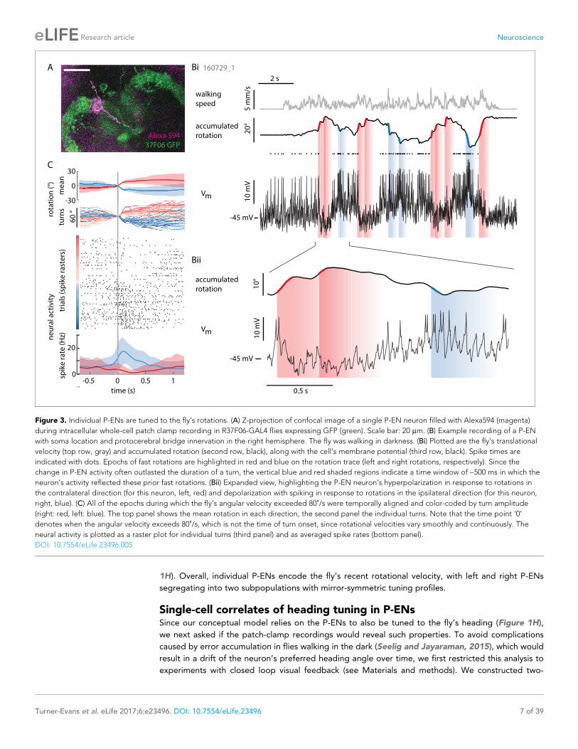
Figure 3. Individual P-ENs are tuned to the fly’s rotations. (A) Z-projection of confocal image of a single P-EN neuron filled with Alexa594 (magenta)

during intracellular whole-cell patch clamp recording in R37F06-GAL4 flies expressing GFP (green). Scale bar: 20 mm. (B) Example recording of a P-EN

with soma location and protocerebral bridge innervation in the right hemisphere. The fly was walking in darkness. (Bi) Plotted are the fly’s translational

velocity (top row, gray) and accumulated rotation (second row, black), along with the cell’s membrane potential (third row, black). Spike times are

indicated with dots. Epochs of fast rotations are highlighted in red and blue on the rotation trace (left and right rotations, respectively). Since the

change in P-EN activity often outlasted the duration of a turn, the vertical blue and red shaded regions indicate a time window of ~500 ms in which the

neuron’s activity reflected these prior fast rotations. (Bii) Expanded view, highlighting the P-EN neuron’s hyperpolarization in response to rotations in

the contralateral direction (for this neuron, left, red) and depolarization with spiking in response to rotations in the ipsilateral direction (for this neuron,

right, blue). (C) All of the epochs during which the fly’s angular velocity exceeded 80˚/s were temporally aligned and color-coded by turn amplitude

(right: red, left: blue). The top panel shows the mean rotation in each direction, the second panel the individual turns. Note that the time point ‘0’

denotes when the angular velocity exceeds 80˚/s, which is not the time of turn onset, since rotational velocities vary smoothly and continuously. The

neural activity is plotted as a raster plot for individual turns (third panel) and as averaged spike rates (bottom panel).

DOI: 10.7554/eLife.23496.005





dimensional tuning maps of P-EN spike rates to rotational velocity and virtual heading, which

revealed localized peaks in firing rate (Figure 5A). We collapsed these maps along either of the two

axes to fit the P-EN’s tuning to the fly’s virtual heading with a compound von Mises function and its

tuning to rotational velocity with a sigmoidal function, as before (Figure 5A, see

Materials and methods). For each cell, we also calculated indices for rotation and heading tuning

(Figure 5B, see Materials and methods), which were, in all but one case (p=0.0676), larger than the

95th percentile of the shuffled control distribution.

-2000200min

max

100

0

-100

an

gu

lar

ve

loci

ty

at

ha

lf m

ax

(°/s

)

ipsi

contra

Ai

R2 = 0.98

100 0 -100

angular velocity (°/s)

0

5

10

15

spik

e r

ate

(H

z)

-1 0 0.5time (s)

-20

0

an

gu

lar

ve

loci

ty (

°/s)

n = 858

-35

-25

Vm

(m

V)

-0.5

10 mV

50 ms

107 msD

B C

L R L R

turn direction

0

5

10

15

spik

e r

ate

(H

z)

spik

e r

ate

(n

orm

aliz

ed

)

Left

Aii

0

10

15

spik

e r

ate

(H

z)

100 0 -100


R2 = 0.87

5

RightLeft

Rightangular velocity (°/s)

contra ipsi

0

0.1

0.2

0.3

ne

ura

l re

spo

nse

lag

(s)

160312_1

Figure 4. Two P-EN subpopulations mirror-symmetrically encode the fly’s rotational velocity. (A) Example tuning curves of P-EN spike rate to the fly’s

rotations as the fly walks in darkness. Angular velocities were binned in 12˚/s bins and a sigmoid was fitted with bin counts used as weights (see

Materials and methods for details). Mean spike rate and 95% confidence interval in black, sigmoidal fits in blue and red. (Ai) Tuning curve for a right

P-EN neuron (same as in Figure 3). P-EN membrane potential changes were similar to the observed changes in spike rates (see Figure 4—figure

supplement 1C for Vm tuning curve). (Aii) Tuning curve for a left P-EN neuron (see Figure 4—figure supplement 2A for example trace). (B) Fitted

spike rates for the flies’ turns to the left versus right illustrate mirror-symmetric tuning properties of the left and right P-EN subpopulations. Spike rates

were computed either at saturation or at an absolute rotational velocity of 200˚/s, whichever was lower. Example cells from panel A are color coded. (C)

Encoding of rotations by the two subpopulations is mirror-symmetric yet overlapping, that is, each P-EN subpopulation encodes rotations in both

directions. Left: Normalized tuning curve fits for all P-EN neurons. Left hemisphere P-EN curves have been reflected for simplicity. Neurons plotted in A

are color coded for comparison. Open circles mark each sigmoid’s half-maximum (inflexion point). Right: On average, the P-EN neurons’ receptive field

for rotations is centered around 0˚/s, where P-EN’s are half-maximally activated. Closed and open circles in the right subplot represent inflexion points

of right and left P-EN tuning curves, respectively. Example cells from panel A are in blue and red. (D) Spike-triggered averages of angular velocities

were constructed to characterize P-EN timing. Since P-EN neurons tend to spike at rest, all spikes with rotational velocities not exceeding 40˚/s at anytime in a one second window around the spike were excluded. Left: Membrane potential is plotted at top, angular velocity at bottom. Inset shows a

magnification of the average spike shape. Right: The peak of the angular velocity precedes the spike in all P-ENs recorded. Example cells from panel A

are in blue and red.

DOI: 10.7554/eLife.23496.006

The following figure supplements are available for figure 4:

Figure supplement 1. Extended data on P-EN rotational velocity tuning.

DOI: 10.7554/eLife.23496.007

Figure supplement 2. Loose patch recordings.

DOI: 10.7554/eLife.23496.008







A

225 0 -200

0

2π

π


he

ad

ing

(ra

d)

225 0 -200angular velocity (°/s)

0

5

spik

e r

ate

(H

z)

0 5spike rate (Hz)

0

2π

π

R2 = 0.87

R2 = 0.94

C160621_1, 55 minutes, 6572 spikes 151129_1, 6 minute epoch, 233 spikes

he

ad

ing

(ra

d)

0

2π

π

R2 = 0.76

R2 = 0.96


0

2π

π

he

ad

ing

(ra

d)


0

10

spik

e r

ate

(H

z)

0 5spike rate (Hz)

10

RightLeft RightLeft

he

ad

ing

(ra

d)

0

4

8

spik

e r

ate

(H

z)

12

B

0 200

count

cou

nt

0

50

shu#ed control

-200

0

200

2π

-60

-40

-20

π0

Dexperiment

vRot

(°/s)

heading

(rad)

Vm

(mV)

2smax

min

max

min

0

0.2

0.4

0 0.5 1

rotation tuning index

he

ad

ing

tu

nin

g in

de

x

Figure 5. P-ENs are conjunctively tuned to angular velocity and heading. (A) Two-dimensional tuning properties of a P-EN’s spike output averaged

over the entire duration of the experiment. The cell was located in the left hemisphere (schematic at top). The fly walked with closed loop visual

feedback. The heat map (upper left) shows spike rates as a function of angular velocity and virtual heading. A tuning curve was fitted to the fly’s virtual

heading angle (upper right) as well as the fly’s angular velocity (lower left) (see Materials and methods). Black: mean rate and 95% confidence intervals.

Tuning curves are least squares fit to the sum of two von Mises functions for heading (green) and to a sigmoidal function for rotations (red). (B)

Quantification of the heading tuning index (mean vector length of spike rates across virtual heading angles) and the rotation tuning index (R2 values for

sigmoidal tuning curve fit) for the two example cells plotted in A and C (bold red open circle and blue open circle, respectively). Shuffled controls (see

Materials and methods) are plotted as dots and dotted lines mark 95th percentile boundaries (plotted in red and blue for the two example cells).

Histograms of shuffled data indices are plotted at top and at right following the same color code. Tuning indices for all cells are shown in Figure 5—

figure supplement 1C. (C) Two-dimensional tuning properties of a P-EN’s spike output during a brief epoch that still sufficiently sampled the two-

dimensional parameter space. The cell was located in the right hemisphere (schematic at top). The fly walked with a closed loop visual feedback. The

heat map (upper left) shows spike rates as a function of angular velocity and virtual heading. Colorbar at right. Tuning curves to the fly’s virtual heading

angle and angular velocity are plotted analogous to A. (D) Example traces for the epoch plotted in C illustrating tuning to rotational velocity as well as

virtual heading. The two parameters are color coded according to the neural activity expected from the tuning curves plotted in panel C.

DOI: 10.7554/eLife.23496.009






P-EN heading tuning was generally stable over time, although we occasionally observed drifts in

the neuron’s preferred heading angle (Figure 5—figure supplement 1A). We assessed tuning stabil-

ity more quantitatively by analyzing short epochs (5–10 min) that sampled a sufficient range of rota-

tional velocities (�250˚/s) across all virtual heading angles (see Materials and methods). We

identified seven such epochs in six different cells recorded in flies walking with closed loop visual

feedback as well as in darkness (see Figure 5C,D for an example and Figure 5—figure supplement

1C for tuning indices, which were, for all but one epoch, larger than the 95th percentile of the shuf-

fled control distributions). For all epochs recorded in flies walking with visual feedback, we found

that the P-ENs’ preferred heading angles during the epochs differed by only 6 ± 5% from the aver-

age of the entire experiment (population mean, N = 4). As a second line of evidence, we found the

P-EN bump width to be roughly similar for short epochs and across whole experiments, suggesting

that a neuron’s preferred heading angle did not drift much over time (average tuning curve width at

half-maximal P-EN heading modulation: 56 ± 20˚ (N = 7 epochs) versus 76 ± 35˚ [N = 5 experiment

averages]). Overall, we found P-EN neurons to be tuned to the fly’s heading as well as the fly’s rota-

tions, both when flies walked under visual closed loop conditions and in darkness (Figure 5—figure

supplement 1C).

Conjunctive tuning to heading and rotation is sharpened withinindividual P-ENsHaving established that P-EN neurons are conjunctively tuned to the fly’s heading and rotations, we

examined our recordings for hints of integrative computations within individual neurons. Specifically,

we began by asking whether P-EN activity was tuned to one of the two parameters even in the

absence of contribution from the other. Figure 6A–B depicts an example of strong P-EN tuning to

rotational velocity as well as to virtual heading for a fly walking in darkness. To quantitatively assess

whether tuning to one parameter depended on the other, we computed the rotation and heading

tuning indices separately for the respective preferred and non-preferred conditions, i.e. one rotation

index each for the fly’s turns within the preferred versus non-preferred heading quadrant and one

heading index each for when the fly rotated in its preferred versus non-preferred turn direction.

These tuning indices were not significantly different (Figure 6C, left). Along the same lines, the pre-

ferred heading angle of individual P-ENs (the mean vector angle of spike rates across headings) was

similar for preferred and non-preferred rotations (Figure 6C, bottom right). Following the same

logic, we also fit conditional tuning curves to subsets of the parameter space (see

Materials and methods for details). As evident from the example (Figure 6D) and the population

data (Figure 6E), strong conjunctive tuning was apparent in the pronounced differences in rate mod-

ulation between preferred and non-preferred conditions. Nevertheless, we found P-EN spiking to be

tuned to rotational velocity in non-preferred heading quadrants and to heading during non-pre-

ferred rotations (Figure 6E left; rotation tuning at non-preferred heading angles: 2.3 ± 2.1 Hz, head-

ing tuning during non-preferred rotations: 1.2 ± 1.1 Hz; one sample t-test: p=0.026 and p=0.043,

respectively; N = 6 for both comparisons). The pronounced conjunctive tuning we observed at the

level of spike rates was less apparent in the subthreshold activity of P-EN neurons (Figure 6—figure

supplement 1). In contrast to the spike rates, for which rate modulation in response to one parame-

ter strongly depended on the other, quantitative modulation of the membrane potential did not

show significant mutual dependence between the two parameters (Figure 6—figure supplement

1C, see Materials and methods for details). These observations suggest not only that tuning of P-EN

output is strongly conjunctive, but also that this property may be sharpened within single P-ENs.

A recurrent loop between P-ENs and E-PGsWe next sought to test the third pillar of our conceptual model, that the E-PG and P-EN neurons are

connected in an excitatory loop. Light level analysis of P-EN neuron morphology suggests that they

Figure 5 continued

The following figure supplement is available for figure 5:

Figure supplement 1. Extended data on P-EN conjunctive tuning.

DOI: 10.7554/eLife.23496.010





A

0

2π

π


he

ad

ing

(ra

d)

160312_1, 5 minute epoch, 576 spikes

spik

e r

ate

(H

z)-1500 200

10

20

30

40

50

0

B2 s

0-200

0200

vRot

(°/s)

2π

heading

(rad)

spikes

0

2π

heading

(rad)

spikes

-2000

200v

Rot (°/s)

D E

0

50

spik

e r

ate

(H

z)

0 2ππ

R2 = 0.67

0

5

10

spik

e r

ate

(H

z)

heading (rad)0 2ππ

R2 = 0.42

-15002000

20

40

spik

e r

ate

(H

z)

R2 = 0.85

-15002000

5

spik

e r

ate

(H

z)


R2 = 0.78


heading (rad)

0

10

20

rota

tio

n t

un

ing

(H

z)

non-pref prefnon-pref pref0

0.5

1

rota

tio

n t

un

ing

ind

ex

non-pref pref0

2π

pre

ferr

ed

an

gle

π

non-pref pref0

0.5

1

he

ad

ing

tu

nin

g in

de

x

headingheading

rotationrotation

C

10

20

he

ad

ing

tu

nin

g (

Hz)

non-pref prefrotation

*p=0.45p=0.86

p=0.66 *

max

min

leftright

*

*

Figure 6. Tuning of P-EN spiking activity is evident even for non-preferred heading and rotational velocities. (A) Heat map shows conjunctive tuning of

a P-EN’s spike output to angular velocity and virtual heading. The fly walked in darkness. (The recording is the same as shown in Figure 4Aii and

Figure 4—figure supplement 2). (B) Example traces from that recording illustrating conjunctive tuning to rotational velocity and virtual heading. The

fly’s rotational velocity is color-coded by preferred (left, blue) and non-preferred (right, red) turn direction. The fly’s heading is color coded according to

the neural activity expected from the heading tuning curve computed from A (see Materials and methods, light green: low, black: high). (C) P-EN spike

output is tuned to rotations irrespective of the fly’s heading (top, R2 value of sigmoidal tuning curve fit) and informative about the fly’s heading

irrespective of rotations, as evident both from the heading tuning index (bottom left, mean vector length of spike rates across virtual heading angles)

and the relative stability of the preferred heading angle (mean vector angle). P-values are results of paired two-sample t-tests. (D) Conditional tuning

curves for the cell plotted in A. Schematics illustrate the subset of data used to construct the tuning curves. Mean and 95% confidence intervals are

plotted in black, fits for preferred conditions in solid and for non-preferred conditions in dotted lines. Top: Tuning to angular velocity given heading

(left: rotations in non-preferred heading quadrant, right: rotations in preferred heading quadrant). Bottom: Tuning to heading given turn direction (left:

non-preferred turn direction, right: preferred turn direction). (E) Strong P-EN conjunctive tuning is apparent from the increased rate modulation for

tuning to one parameter in the preferred range of the other. Top: Difference in fitted spike rates at �150 and 150˚/s for each condition (two sample

t-test: p=0.049, N = 6). Bottom: Difference in fitted spike rates at the heading angles corresponding to the peak and the trough of the unconditional

heading tuning curve (two sample t-test: p=0.042, N = 6). Tuning to rotations in non-preferred heading quadrants (top left) and tuning to heading

during non-preferred rotations (bottom left) is, however, significantly different from zero (one sample t-test: p=0.026 and p=0.043, respectively). Filled

circles are recordings in darkness; open circles, in visual closed loop. Color code is the same as used in Figure 5—figure supplement 1C. p<0.05.

DOI: 10.7554/eLife.23496.011


Figure supplement 1. P-EN spiking activity shows stronger conjunctive tuning than membrane potential.

DOI: 10.7554/eLife.23496.012






likely have post-synaptic specializations in the bridge and pre-synaptic boutons in the ellipsoid body,

while E-PG morphology indicates the opposite polarity (Wolff et al., 2015), making it possible for

the two cell types to be mutually connected. We sought histochemical confirmation of this polarity

by expressing the presynaptic reporter synaptotagmin-smGFP-HA (Aso et al., 2014) in GAL4 lines

that drive expression in P-EN and E-PG neurons, respectively. Light level analysis of brains in which

HA-tagged synaptotagmin was expressed in P-EN neurons revealed stronger labeling in the ellipsoid

body and noduli than in the bridge (Figure 7A, 11/14 brains). In contrast, analysis of the E-PG tar-

geted brains revealed high levels of HA-tagged synaptotagmin in the protocerebral bridge, but also

in the ellipsoid body (at higher levels than in the ellipsoid body in 5/15 brains, at comparable levels

in both neuropils in 10/15 brains, see Figure 7B). These results are consistent with the anatomical

finding that the P-EN neurons receive input in the bridge and send output to the ellipsoid body.

To confirm these key connections, we then performed functional connectivity experiments

between the two neuronal subtypes in ex vivo preparations. We expressed the red-shifted channelr-

hodopsin CsChrimson (Klapoetke et al., 2014) in either the E-PG or the P-EN populations while

expressing GCaMP6m or GCaMP6f in the putative downstream partner cell type. Optogenetic acti-

vation of P-EN neurons reliably evoked positive calcium transients in E-PG neurons (Figure 7C, see

Materials and methods), suggesting that angular velocity information is indeed relayed to E-PGs via

this pathway. However, activation of the E-PG population induced more variable responses in P-ENs.

Although we observed responses consistent with excitatory connections when we used strong light

intensities for optogenetic activation (Figure 7D), the same pairing evoked activation, inhibition, and

a lack of response at different times with weaker light intensities (dotted line in Figure 7D, inset).

Thus, the excitatory loop between E-PG and P-EN neurons may be both direct and indirect, and the

connection from the E-PG neurons onto the P-EN neurons likely also recruits inhibition. Overall, we

hypothesize that other neurons in the ellipsoid body and protocerebral bridge (Wolff et al., 2015)

likely influence the exchange of information between these two neuron types.

P-EN calcium activity in the protocerebral bridge follows E-PG activityConsistent with our conceptual model (Figure 1H), our electrophysiological results showed that indi-

vidual P-EN neurons are tuned to heading and rotational velocity. Further, our functional connectivity

results are supportive of a recurrent loop between the P-EN and E-PG populations, albeit perhaps

with greater complexity than proposed by our simple conceptual model. This loop would, in the

model, imply that the P-EN population inherits a bump of activity from the output of the E-PG popu-

lation in the bridge, and that P-EN activity leads the E-PG bump in the ellipsoid body. To understand

the spatiotemporal relationship between the two populations, we performed two-color calcium

imaging (Dana et al., 2016) in flies walking in darkness. We expressed GCaMP6f in one population

and jRGECO1a, a red indicator, in the other (Figure 8A). We tested for bleed-through and cross talk

between the two channels (Sun et al., 2017), and verified clean color channel separation (see Fig-

ure 8—figure supplement 1 and Materials and methods for details; Sun et al., 2017). We also

checked that our results were qualitatively consistent across the calcium indicator combinations we

used and pooled the data for both color combinations in the results presented below, color-coding

data according to the calcium indicator with which they were obtained in Figure 8.

Imaging in the protocerebral bridge revealed two bumps of activity in the E-PG and P-EN neu-

rons, one on each side of the bridge (Figure 8B), as predicted by our working model. To analyze the

imaging stacks, we subdivided each half of the protocerebral bridge into nine regions of interest,

one for each glomerulus (Figure 8C) and compared the activity in those regions over time to the

rotational velocity for single trials (Figure 8D) and across trials (Figure 8E). For both neuron types,

the bump intensities, but not widths, increased with increasing angular velocity across trials

(Figure 8E,F). Although the P-EN bump intensity increased for both turn directions, which was unex-

pected, the increase was larger for ipsilateral turns than for contralateral turns (Figure 8—figure

supplement 2A, top), a mirror-symmetry consistent with imaging results in the noduli (Figure 2) and

with single cell electrophysiology (Figure 4B). The bump half-widths spanned ~2 glomeruli, which, if

projected to the ellipsoid body, would lead to an activity width of 90 degrees. Consistent with our

model, in which E-PG neurons carry the heading representation to the protocerebral bridge

(Figure 1H), and in contrast with the activity of the P-EN subpopulations, there was no difference

between E-PG activity for ipsilateral versus contralateral turns at any turn velocity (Figure 8—figure

supplement 2A, bottom).




To determine the spatiotemporal relationship of the E-PG and P-EN bumps, we carefully exam-

ined their relative positions over time and across rotational velocities. To facilitate this comparison,

we simultaneously registered both populations with respect to the E-PG bump in the right half of

the bridge. We then binned these registered traces by rotational velocity. Across velocities, the reg-

istered E-PG and P-EN activity bumps overlapped, but with the P-EN bumps slightly lagging the

P-EN - CsChrimson; E-PG - GCaMP6m

E-PG - CsChrimson; P-EN - GCaMP6fCi Di

Cii

2 s

10

% ∆

F/F

Dii

B E-PG membrane marker presynaptic marker

A P-ENmembrane marker presynaptic marker

P-EN

E-PG

E-PG

P-ENE-PG

P-EN

Figure 7. Functional connectivity of E-PG and P-EN neurons. (A) P-EN neuron membranes and presynaptic sites are labeled by expressing myr-sm::GFP

and synaptotagmin in VT008135-GAL4, a second genetic line that drives expression in the P-EN neurons. While additional central complex and central

brain cell types are targeted in this line, only the P-EN neuron arborizes in the protocerebral bridge (see Materials and methods). Expression is evident

in the protocerebral bridge, the ellipsoid body and the paired noduli (behind the ellipsoid body, labelled by arrowhead). Intensity of presynaptic

labeling was strongest in the ellipsoid body. The scale bar is 20 mm and applies to A and B. Though the image stack was rotated in three dimensions to

obtain the included view, the scale bar was obtained from a single plane of the imaging stack. (B) Analogous to A, but using R60D05-GAL4 to drive

expression in the E-PG neurons. Although presynaptic labeling was most intense in the protocerebral bridge and gall, synaptotagmin was also

detected in the ellipsoid body, suggesting E-PG presynaptic sites in that neuropil as well. (C) Functional connectivity experiment with CsChrimson-

mCherry expressed in P-EN, and GCaMP6m in E-PG neurons. (Ci) (Left) Average projection of fluorescence from a dissected brain. Both E-PG and P-EN

arborizations can be seen in the ellipsoid body. E-PGs furthermore project to the gall (box, left) and P-ENs to the noduli (paired structure at bottom).

(Right) Average frame from imaging the E-PGs in the gall while activating the P-ENs. (Cii) Average response (in black) from six flies to a train of 2 ms,

590 nm light pulses delivered at 30 Hz and 50 mW/mm2. Stimulation time indicated by gray area. Gray traces correspond to the average of 4 trials for

individual flies. (D) Functional connectivity experiment with CsChrimson-mCherry expressed in E-PG and GCaMP6f in P-EN neurons. (Di) (Left) Average

projection of fluorescence from a dissected brain. (Right) Average frame from imaging the P-ENs in the protocerebral bridge while activating the

E-PGs. (Dii) Analogous to Cii, except that stimulation light intensity was increased to 500 mW/mm2. (inset) Comparison of low stimulation intensity

responses (50 mW/mm2, dotted line) and the high stimulation responses shown in the plot below (solid line). These responses were acquired in different

regions (low stimulation: noduli, high stimulation: protocerebral bridge), but results were consistent across neuropiles. The scale bars are scaled

versions of those shown in Cii. All scale bars in Ci, Di: 10 mm.

DOI: 10.7554/eLife.23496.013





23 o/s

85 o/s

79 o/s

%ΔF/F

0

75

jRGECO1a GCaMP6f

A

0

66

0

550F

0

150

vRot 9 ... 11 ... 9

C D

E

911

9

E-PG P-EN

t1

t2

t3

G

0

1

2

3

FW

HM

(#

of

glo

m.)

vRot

(o/s)

B

0

80

0

100

0

75

0

150

t1- t

3

GCamp6fjRGECO1a

E-PG P-EN

L R

activity map

VRot

bins: F

FWHM

%ΔF/F

%ΔF/F

vR

ot (

°/s) 180

-180

0

time (s)10 20 30

E-P

GP

-EN

9

9

11

R

L

9

9

11

R

L

...

...

...

...

15 75 135

-1

0

1

2

Ipsi

Contra

vRot

(o/s)

0.05

0

15 45 75 105 135

P-EN

PVA stren.

... ...

10

0%

ΔF

/F

4 glom.

0-45 o/s 45-90 o/s 90-135 o/s 135-180 o/s

vRot

(o/s)15 75 135

%ΔF/F

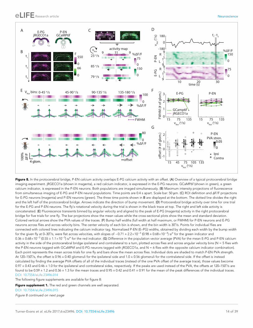
Figure 8. In the protocerebral bridge, P-EN calcium activity overlaps E-PG calcium activity with an offset. (A) Overview of a typical protocerebral bridge

imaging experiment. jRGECO1a (shown in magenta), a red calcium indicator, is expressed in the E-PG neurons. GCaMP6f (shown in green), a green

calcium indicator, is expressed in the P-EN neurons. Both populations are imaged simultaneously. (B) Maximum intensity projections of fluorescence

from simultaneous imaging of E-PG and P-EN neural populations. Time points are 0.4 s apart. Scale bar: 50 mm. (C) ROI definition and DF/F projections

for E-PG neurons (magenta) and P-EN neurons (green). The three time points shown in B are displayed at the bottom. The dotted line divides the right

and the left half of the protocerebral bridge. Arrows indicate the direction of bump movement. (D) Protocerebral bridge activity over time for one trial

for the E-PG and P-EN neurons. The fly’s rotational velocity during the trial is shown in the black trace at top. The right and left side activity is

concatenated. (E) Fluorescence transients binned by angular velocity and aligned to the peak of E-PG (magenta) activity in the right protocerebral

bridge for five trials for one fly. The bar projections show the mean values while the cross-sectional plots show the mean and standard deviation.

Colored vertical arrows show the PVA values of the traces. (F) Bump half widths (full width at half maximum, or FWHM) for P-EN neurons and E-PG

neurons across flies and across velocity bins. The center velocity of each bin is shown, and the bin width is 30˚/s. Points for individual flies areconnected with colored lines indicating the calcium indicator tag. Normalized P-EN (E–PG) widths, obtained by dividing each width by the bump width

for the given fly at 0–30˚/s, were flat across velocities, with slopes of �0.71 ± 2.2�10�3 (0.98 ± 0.68�10�3) s/˚ for the green indicator and

0.36 ± 0.68�10�3 (0.55 ± 1.1�10�3) s/˚ for the red indicator. (G) Difference in the population vector average (PVA) for the mean E-PG and P-EN calcium

activity in the side of the protocerebral bridge ipsilateral and contralateral to a turn, plotted across flies and across angular velocity bins (N = 5 flies with

the P-EN neurons tagged with GCaMP6f and E-PG neurons tagged with jRGECO1a, and N = 6 flies with the opposite calcium indicator combination).

Each point represents the mean across trials for one fly and bars show the mean across flies. Individual dots are shaded to match P-EN PVA strength.

At 120–150˚/s, the offset is 0.96 ± 0.40 glomeruli for the ipsilateral side and 1.0 ± 0.56 glomeruli for the contralateral side. If the offset is instead

calculated by finding the average PVA offsets of all of the individual traces (instead of the one PVA offset of the average trace), those values become

0.97 ± 0.43 and 0.46 ± 1.0 for the ipsilateral and contralateral sides, respectively. If the peaks are used instead of the PVA, the offsets at 120–150˚/s arefound to be 0.59 ± 1.2 and 0.36 ± 1.3 for the mean traces and 0.95 ± 0.42 and 0.41 ± 0.91 for the mean of the peak differences of the individual traces.

DOI: 10.7554/eLife.23496.014


Figure supplement 1. The red and green channels are well separated.

DOI: 10.7554/eLife.23496.015







E-PG bumps (Figure 8E,G, see Materials and methods for further details on the registration and bin-

ning procedures). The lag led to bump offsets of approximately one glomerulus (the equivalent of

45 degrees in the ellipsoid body) at 120–150˚/s, the fastest rotational velocity bin considered (and

the bin with the greatest offset), whether measured by the population vector average or by peak dif-

ference (Figure 8G). This offset was also consistent across different fly lines (Figure 8—figure sup-

plement 2B). While the substantial overlap between the two bumps suggests that the heading

representation in the two populations is, in fact, roughly coincident, the observation that P-EN activ-

ity follows E-PG activity by one glomerulus on both sides of the bridge was not predicted by our

simple model. This lag may be due to the subtleties of connectivity between the E-PG neurons and

P-EN neurons (as hinted at, for example, by E-PG presynaptic specializations in the ellipsoid body

[Figure 7B] and by the complex responses seen in our functional connectivity experiments

[Figure 7D, inset]) or, simply, due to delays caused by neural time constants (see model below).

P-EN calcium activity in the ellipsoid body leads E-PG activityNext, we sought to investigate the relationship of the P-EN and E-PG population activity in the ellip-

soid body, where, the conceptual model would suggest (Figure 1H), P-EN activity should lead E-PG

activity. To do so, we once again performed two-color imaging of the two populations (Figure 9A).

As in the protocerebral bridge, we observed bumps of activity in both neural populations

(Figure 9B). We then subdivided the activity into 16 regions of interest, corresponding to the num-

ber of distinct E-PG arborization sectors in the ellipsoid body (Figure 9B, bottom; [Wolff et al.,

2015]) and compared the activity in those regions over time (Figure 9C). Bump amplitudes, but not

half-widths, varied with angular velocity (Figure 9D,E), and both bumps were ~100˚ wide (full width

at half maximum, Figure 9E).

To compare E-PG and P-EN bump positions in the ellipsoid body across time, we performed a

registration and binning procedure similar to the one used in the protocerebral bridge (see

Materials and methods). Here, we used the E-PG bump in the ellipsoid body to align averaged cal-

cium transients binned by the fly’s angular velocity (Figure 9F, standard deviations shown in Fig-

ure 9—figure supplement 1). As the fly turned, the relative position of the E-PG and P-EN bumps

around the ellipsoid body changed. At angular velocities less than 30˚/s, all flies showed bump off-

sets of less than 6˚ (2.5 ± 2.1˚, N = 10 flies, Figure 9F,G). However, at rotational velocities above

30˚/s, P-EN population activity separated from E-PG activity, with the P-EN bump leading the E-PG

bump around the ellipse (Figure 9G, Video 2). When the red indicator was expressed in the E-PG

neurons and the green indicator in the P-EN neurons, the bump offset exceeded 15 degrees of sep-

aration for turns faster than 90˚/s regardless of turn direction and regardless of whether the fly was

angularly accelerating or decelerating (20.7 ± 11.7˚ at 150–180˚/s). When, instead, the red indicator

was expressed in the P-ENs, the lead-lag behavior was qualitatively similar, though the shift only

rose to 7.3 ± 7.2˚/s at 150–180˚/s (Figure 9—figure supplement 2). As jRGECO1a’s kinetics are dif-

ferent from those of GCaMP6f, a difference in the observed shift across color combinations is to be

expected (Dana et al., 2016). Thus, we concluded that the P-EN bump leads the E-PG bump in the

ellipsoid body during turns, consistent with the conceptual model.

Firing rate model captures interaction of angular velocity and compasssignalsOur conceptual model (Figure 1H) suggested that the anatomical offset between the E-PG and

P-EN populations would move the activity bump in both populations during turns, thereby integrat-

ing rotational velocity to compute heading. However, it offered few predictions for how the feed-

back loops in the circuit might shape bump dynamics. In our two-color imaging experiments, we

observed the hypothesized P-EN to E-PG activity offset, but the shift was small, between 10˚ and30˚ at the highest angular velocities. Further, the E-PG activity in the bridge was consistently

advanced from the P-EN activity by an offset that could exceed one glomerulus, which is half of the

Figure 8 continued

Figure supplement 2. Additional quantification of protocerebral bridge activity.

DOI: 10.7554/eLife.23496.016





B

FG

D

0

85F

0-60 o/s 60-120 o/s 120-180 o/s 120-60 o/s 60-0 o/s

0

50

100

150

FW

HM

(o)

0

50

100

150

FW

HM

(o)

E

P-EN

1

1.5

2

2.5

no

rm. p

ea

k m

ax

E-PG

0.8

1.2

1.6

2

no

rm.

pe

ak

ma

x

-21 o/s

148 o/s

70 o/s

0

750

t1

t2

t3

-10

0

10

20

30

PV

A d

i!e

ren

ce (

o)

0.12

0

PVA strengthP-ENE-PG

61.0o

A

E-PG

P-EN

jRGECO1a

GCaMP6f

∆t = 0.4 s

C

vRot

increasing vRot

decreasing

vRot

range:

15 45 75105

135165

vRot

(o/s)

15 45 75105

135165

vRot

(o/s)

%ΔF/F

0

100

0

100F 15 45 75105

135165

vRot

(o/s)

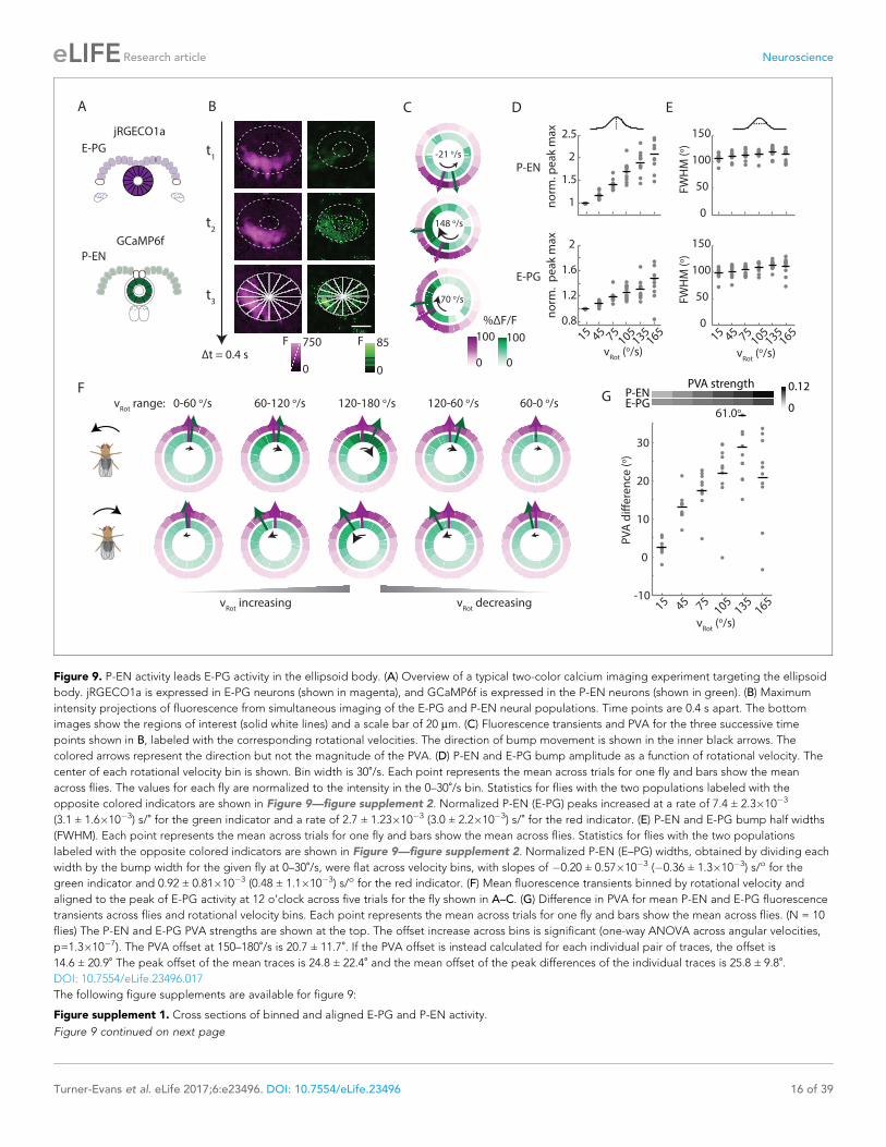
Figure 9. P-EN activity leads E-PG activity in the ellipsoid body. (A) Overview of a typical two-color calcium imaging experiment targeting the ellipsoid

body. jRGECO1a is expressed in E-PG neurons (shown in magenta), and GCaMP6f is expressed in the P-EN neurons (shown in green). (B) Maximum

intensity projections of fluorescence from simultaneous imaging of the E-PG and P-EN neural populations. Time points are 0.4 s apart. The bottom

images show the regions of interest (solid white lines) and a scale bar of 20 mm. (C) Fluorescence transients and PVA for the three successive time

points shown in B, labeled with the corresponding rotational velocities. The direction of bump movement is shown in the inner black arrows. The

colored arrows represent the direction but not the magnitude of the PVA. (D) P-EN and E-PG bump amplitude as a function of rotational velocity. The

center of each rotational velocity bin is shown. Bin width is 30˚/s. Each point represents the mean across trials for one fly and bars show the mean

across flies. The values for each fly are normalized to the intensity in the 0–30˚/s bin. Statistics for flies with the two populations labeled with the

opposite colored indicators are shown in Figure 9—figure supplement 2. Normalized P-EN (E-PG) peaks increased at a rate of 7.4 ± 2.3�10�3

(3.1 ± 1.6�10�3) s/˚ for the green indicator and a rate of 2.7 ± 1.23�10�3 (3.0 ± 2.2�10�3) s/˚ for the red indicator. (E) P-EN and E-PG bump half widths

(FWHM). Each point represents the mean across trials for one fly and bars show the mean across flies. Statistics for flies with the two populations

labeled with the opposite colored indicators are shown in Figure 9—figure supplement 2. Normalized P-EN (E–PG) widths, obtained by dividing each

width by the bump width for the given fly at 0–30˚/s, were flat across velocity bins, with slopes of �0.20 ± 0.57�10�3 (�0.36 ± 1.3�10�3) s/o for the

green indicator and 0.92 ± 0.81�10�3 (0.48 ± 1.1�10�3) s/o for the red indicator. (F) Mean fluorescence transients binned by rotational velocity and

aligned to the peak of E-PG activity at 12 o’clock across five trials for the fly shown in A–C. (G) Difference in PVA for mean P-EN and E-PG fluorescence

transients across flies and rotational velocity bins. Each point represents the mean across trials for one fly and bars show the mean across flies. (N = 10

flies) The P-EN and E-PG PVA strengths are shown at the top. The offset increase across bins is significant (one-way ANOVA across angular velocities,

p=1.3�10�7). The PVA offset at 150–180˚/s is 20.7 ± 11.7˚. If the PVA offset is instead calculated for each individual pair of traces, the offset is

14.6 ± 20.9˚ The peak offset of the mean traces is 24.8 ± 22.4˚ and the mean offset of the peak differences of the individual traces is 25.8 ± 9.8˚.DOI: 10.7554/eLife.23496.017


Figure supplement 1. Cross sections of binned and aligned E-PG and P-EN activity.






typical bump full width at half maximum in the protocerebral bridge. Finally, our functional connec-

tivity experiments suggested that E-PG to P-EN connections may involve not just direct excitation,

but the likely recruitment of inhibition as well. Thus, the simple conceptual model could not suffi-

ciently explain the circuit dynamics we observed.

We therefore designed and simulated a firing rate model that built on the known facts about the

circuit’s topology. We separated the P-EN neurons into two subpopulations of nine neurons each

(one neuron per protocerebral bridge glomerulus, see Materials and methods), one population for

neurons with dendritic projections on the right side of the protocerebral bridge, and another for

neurons with dendritic projections on the left side. 54 E-PG neurons (three neurons per protocere-

bral bridge glomerulus) locally excite P-EN neurons, with each P-EN neuron innervating one glomer-

ulus of the protocerebral bridge. In return, P-EN neurons excite E-PG neurons in the ellipsoid body,

but with a shift in either the clockwise or coun-

terclockwise direction, depending on whether

they belong to the left or the right subpopula-

tion. Further, we stipulated that the E-PG neu-

rons uniformly and strongly inhibit P-EN neurons

(all connections shown in Figure 10A; see Fig-

ure 10—figure supplement 1A for the connec-

tivity matrix; see Discussion for possible

inhibitory pathways). Such inhibition was a pre-

requisite to obtain a stationary bump of activity

and a near-linear integration of velocity inputs

(Figure 10—figure supplement 1B; see below).

Finally, turns were initiated by an external input

to the model that uniformly excites either the

right or left P-EN subpopulations (Figure 10A,

bottom).

This rate model, which is reminiscent of past

models of mammalian head direction cells

(Skaggs et al., 1995; Xie et al., 2002;

Zhang, 1996), albeit with key differences in con-

nectivity, captured the essence of much of what

we observed in our experiments. Simulated fir-

ing rate curves of P-ENs in response to rotational

velocity input were sigmoidal with an inflexion

point at 0˚/s, matching our experimental obser-

vations (compare Figure 10—figure supple-

ment 1C and Figure 4C). Further, the

simulations indicated that the circuit functions as

a ring attractor, enforcing a unique bump across

the E-PG population, consistent with previous

experimental results (Seelig and Jayaraman,

2015, Kim et al., 2017) (Figure 10B,C). Our

model does not feature an attractor network

within the E-PG population. Rather, E-PG activity

is driven entirely by P-EN neurons and the per-

sistent bump of activity arises from a feedback

loop between these two neural populations. As

a result, the activity and bump amplitudes of

Figure 9 continued

DOI: 10.7554/eLife.23496.018

Figure supplement 2. Statistics of P-EN and E-PG activity in the ellipsoid body for flies with the opposite calcium indicator combination.

DOI: 10.7554/eLife.23496.019

Video 2. P-EN bump leads the E-PG bump in the

ellipsoid body. Example of two-color calcium imaging

in the ellipsoid body of a fly walking on a ball. Part 1.

(Top) Red channel signal from the E-PG neurons. The

outline of the E-PG arborizations in the ellipsoid body

is marked with dotted white lines. The heading of the

fly, as read out from the ball position, is shown by the

white circle. The population vector average of the

activity is labeled by the magenta line. (Bottom) Video

of the fly on the ball. Part 2. (Top) Green channel signal

from the P-EN neurons. The outline of the P-EN

arborizations in the ellipsoid body is marked with

dotted white lines. The amplitude of the rotational

velocity is indicated by the white bar at right. The

population vector average is labeled with the green

line. (Bottom) Video of the fly on the ball. Part 3. (Top)

Combined red and green activity and PVA of both the

E-PG and P-EN neurons. (Bottom) Video of the fly on

the ball.

DOI: 10.7554/eLife.23496.020







both populations are sensitive to velocity input, as observed experimentally (Figure 10—figure sup-

plement 1C,D).

The firing rate model also produced offsets in the activity of the E-PG and P-EN neurons in the

ellipsoid body and in the protocerebral bridge, qualitatively matching our experimental observa-

tions. In the simulations, the offsets are due to the neural time constants (see

G

err

or

va

ria

nce

(ra

d2)

F

simulated PVA

DAmodel

inhibitory:

excitatory:

input:

Bellipsoid body

C protocerebral bridge

E

E-PG

P-EN rightP-EN left

E-PG

P-EN rightP-EN left

P-EN rightP-EN left

left turn right turn

P-EN left

P-EN rightP-EN sum

E-PGright PB

left PB

ellipsoid body

0 20 40 60 80 100

time (s)

0

π

he

ad

ing

(ra

d)

0 200

rotational velocity (º/s)

0

50

100

150

200

bu

mp

ve

loci

ty (

º/s)

0 200

rotational velocity (º/s)

−15

−10

−5

0

5

10

15

− π 0 πangle (rad)

0.0

0.1

− π 0 π

angle (rad)

0.00

0.05

− π 0 πangle (rad)

0.0

0.1

− π 0 π

angle (rad)

0.00

0.05

time (s)

10 1000

10

1

0.1

0.01

E-PG in left PB

E-PG in right PB

simulation simulation

heading

°)

Figure 10. Firing rate model for a circuit mechanism displaying persistent localized activity and angular velocity integration. (A) Schematic of effective

excitatory (top) and inhibitory (middle) connectivity assumed in the firing rate model and external inputs to the P-EN populations (bottom). Note the

anatomical shift in the ellipsoid body between E-PG and P-EN neurons relative to their protocerebral bridge connections. We assume one P-EN and

three E-PG neurons per protocerebral bridge glomerulus. (B) Activity of E-PG and P-EN neurons in the ellipsoid body for counterclockwise turns at low

(left, 35˚/s) and high—that is, close to saturation— (right, 190˚/s) angular velocities. (C) Activity of E-PG and P-EN neurons in the protocerebral bridge at

low (left) and high (right) angular velocities for a snapshot in time. The velocities are the same as in B. (D) PVA difference between P-EN and E-PG

bumps in the ellipsoid body (black) or protocerebral bridge (red, blue) for different angular velocities for counterclockwise turns. (E) E-PG bump velocity

as a function of the fly’s rotational velocity. The bump velocity displays saturation at high velocities. A linear fit of slope one around the origin is also

displayed (upward shifted for display purposes). Rotational velocities along this line will be reliably integrated. (F) Simulated PVA of the E-PG

population as a function of time for a time varying rotational velocity input (see Figure 10—figure supplement 2 for a description of the input). (G)

Evolution of the estimator of the error variance between the velocity input and the simulated PVA. Beyond 10 s, the statistics of the discrepancy follow a

diffusion equation with a diffusion coefficient of 1.82 � 10�3 rad2/s (see Materials and methods for a description of the fitting procedure). The shaded

area indicates the standard deviation of the estimator.

DOI: 10.7554/eLife.23496.021


Figure supplement 1. Model connectivity and performance.

DOI: 10.7554/eLife.23496.022

Figure supplement 2. Angular velocity statistics.

DOI: 10.7554/eLife.23496.023







Materials and methods); the bump in the P-EN population is not updated immediately after the

E-PG bump shifts. We thus observe a phase difference in the bridge, with the P-EN bumps lagging

the E-PG bumps, as observed experimentally (Figure 8G). This lead-lag relationship was reversed in

the ellipsoid body, where the P-EN population drives the E-PG population. The neural constants are

expected to be largely independent of the bump’s velocity. Consequently, when the E-PG bump in

the protocerebral bridge, for instance, traveled further in a given time window (as during a fast

turn), the P-EN bump lag and phase difference increased, consistent with experimental observations

(Figure 9F, Figure 10D).

For an animal to reliably track its heading over long periods of time, it must accurately integrate

its rotational velocity. Thus, in a robust system, the heading representation should update with an

internal rotational velocity that matches the animal’s external velocity. Indeed, the architecture of

our model ensures a quasi-linear relationship between bump rotation and steady velocity input

(Figure 10E) up to an inherent saturating angular velocity. This linearity mainly depends on an

appropriate balance of local E-PG to P-EN excitation, and inhibition onto the P-EN neurons (Fig-

ure 10—figure supplement 1B). When we drove the P-ENs with a simulated but realistic time vary-

ing velocity input (Figure 10—figure supplement 2), we saw that the bump in the model closely

followed the integrated external velocity, reliably tracking the animal’s heading (see Figure 10F, Fig-

ure 10—figure supplement 1E,F). The errors that did arise were due to inaccurate integration of

small input velocities. The limited number of P-EN neurons in the model (nine per subpopulation)

caused the bump to ‘stick’ at individual P-EN neurons until the input velocity provides enough drive

to free it, at values greater than 15˚/s. The integration error, the difference between the bump posi-

tion and the integrated velocity input, followed a distribution centered on zero, with a variance that

increased over time (see Materials and methods). For short times (on the order of 10 s or less), the

variance of the distribution was small, that is, the error between the animal’s heading and the ani-

mal’s representation of its heading was likely to be small (Figure 10—figure supplement 1E). This

error was influenced by the neural time delays of the angular integration circuit (Figure 10—figure

supplement 1F). For longer time scales, the error distribution broadened (Figure 10G) so that the

variance increased linearly, a characteristic feature of a diffusion process (that is, the heading repre-

sentation diffused away from the true heading over time). Overall, the linearity of the heading

response to input and the small value of the diffusion coefficient suggest that this simple model of

only three neural populations and E-PG to P-EN inhibition, which may be mediated by an additional

and as-yet-uncharacterized neural population, can not only maintain a bump of activity, but can accu-

rately update that bump position to reflect the animal’s heading.

Blocking the P-EN synaptic output alters the E-PG activityBoth the conceptual model (Figure 1H) and the quantitative model (Figure 10) rely on P-EN input

to the E-PG neurons to maintain and move the bump. To assess the impact of the loss of P-EN input

on E-PG bump strength and movement, we imaged E-PG activity while impairing P-EN synaptic

transmission. To that end, we used shiTS, a temperature-sensitive mutation of the Drosophila gene

encoding a dynamin orthologue, which blocks vesicle endocytosis at elevated temperatures (Kita-

moto, 2001). We compared E-PG activity between control flies expressing shiTS in an empty pro-

moter Gal4 and flies expressing shiTS in two different P-EN lines, R37F06 and VT008135. For each

line, we compared the activity at room temperature (permitting synaptic transmission) to the activity

at the restrictive temperature of 31˚C, where vesicle reuptake and, thus, synaptic transmission should

be blocked (Figure 11).

We first checked that the flies’ behavior was consistent across genotypes. Indeed, the walking

statistics were similar at a given temperature across GAL4 lines (see, for example, the distributions

for two flies at 31˚C in Figure 11Ai), though we consistently observed a strong increase in forward

walking at the higher temperature (Figure 11Aii). In experiments with control flies, we found that

this increased forward velocity reliably led to a high-amplitude E-PG activity bump at the higher tem-

perature (Figure 11B, top). As expected, the bump position slowly drifted away from the fly’s head-

ing in darkness, but otherwise tracked the fly’s rotations (Figure 11B, bottom). In contrast, in flies

that expressed shiTS in P-EN neurons, the bump was significantly weaker and more variable

(Figure 11C), although these flies walked just as actively at the higher temperature as control flies.

We next quantified the effects of blocking P-EN neurons on E-PG bump amplitude. At room tem-

perature, the distribution of E-PG bump amplitude across trials was similar for the control flies and




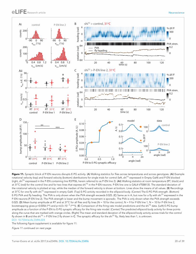
20 40 60 80 100 120time (s)

rota

tio

n (

rad

)

0

he

ad

ing

(ra

d)

-π

π

0

-6π

6π

0

-π

π

% ΔF/F

0

300

PVA stren.

0

0.2

shiTS > control, 31oC

shiTS > P-EN line 2, 31oC

Figure 11

B

C

D

Ai

0.5

1

vF

or (

cm/s

)

0

45

90

vR

ot s

.d.

(o/s

)

RT 31oC

control

RT 31oC RT 31oC0

20 40 60 80 100 120time (s)

% ΔF/F

0

200

PVA stren.

0

0.2

PVA

rota

tio

n (

rad

)h

ea

din

g (

rad

)

0

-6π

6π

E

0

50

100

150

bu

mp

am

pli

tud

e (

% Δ

F/F

)

RT 31oC RT 31oC RT 31oC

control P-EN line 1 P-EN line 2

*****

0

100

0

100

angle (rad)0 π 2π

model

P-EN line 2

control

% Δ

F/F

data

0 0.4 0.8 1.2

vFor

(cm/s)

-90 0 90v

Rot (o/s)

0 0.4 0.8 1.2

vFor

(cm/s)

0

100

200

cou

nts

-90 0 90v

Rot (o/s)

0

200

cou

nts

P-EN line 2control

Aii

P-EN line 1 P-EN line 2

0.0

0.1

A. U

.

0 π 2 π0.0

0.1

0.0

0.1

angle (rad)0.0 0.5 1.0

0.00

0.02

0.04

0.06

0.08

0.10

E-P

Gs

am

pli

tud

e (

A. U

.)

Figure 11. Synaptic block of P-EN neurons disrupts E-PG activity. (A) Walking statistics for flies across temperatures and across genotypes. (Ai) Example

rotational velocity (top) and forward velocity (bottom) distributions for single trials for control (left, shiTS expressed in Empty Gal4) and P-EN blocked

(right, shiTS expressed in the P-EN containing line R37F06, herein referred to as P-EN line 2). (Aii) Walking statistics at room temperature (RT, black) and

at 31˚C (red) for the control line and for two lines that express shiTS in the P-EN neurons. P-EN line one is GAL4-VT008135. The standard deviation of

the rotational velocity is plotted at top, while the median of the forward velocity is shown at bottom. Lines show the means of all values. (B) Recordings

at 31˚C for one fly with shiTS expressed in empty Gal4. (Top) E-PG activity recorded in the ellipsoid body. (Center) The E-PG PVA strength. (Bottom)

E-PG PVA and fly heading. The PVA is only shown when the PVA strength exceeds 0.025. (C) Same as in A, but now for a fly with shiTS expressed in the

P-EN neurons (P-EN line 2). The PVA strength is lower and the bump movement is sporadic. The PVA is only shown when the PVA strength exceeds

0.025. (D) Mean bump amplitude at RT and at 31˚C for all flies and fly lines (N = 10 for the control, N = 9 for P-EN line 1, N = 10 for P-EN line 2,

bootstrapping gives p=0.0056 (**) and p=6.0�10�4 (***)). (E) Comparison of the firing rate model predictions and the shiTS data. (Left) E-PG bump

amplitude as a function of the P-EN to E-PG synaptic efficacy for the firing rate model. (Center) The predicted ellipsoid body activity for three points

along the curve that are marked with orange circles. (Right) The mean and standard deviation of the ellipsoid body activity across trials for the control

fly shown in B and the shiTS > P-EN line 2 fly shown in C. The synaptic efficacy for the shiTS fly, likely less than 1, is unknown.

DOI: 10.7554/eLife.23496.024







for flies that expressed shiTS in the P-EN neurons (Figure 11D). At 31˚C, however, when the flies

became more active and increased their forward velocity, the amplitude distribution of the control

flies shifted to higher values. In contrast, in the shiTS P-EN flies, where this activity increase was

accompanied by a synaptic block in P-EN neurons, the bump amplitude distribution remained rela-

tively unchanged, or even decreased (Figure 11D).

We looked to see if this reduced amplitude could be explained by our firing rate model. The

model demonstrated that two recurrent E-PG/P-EN loops are sufficient to maintain and shift a bump

of activity (Figure 10). If connections between the model’s loops are broken, the bump would be

expected to disappear. To explore the consequences of weakening the P-EN to E-PG connections

instead of breaking them entirely, we continuously tuned the weights down to 0 from their initial

value (thereby modifying the P-EN to E-PG synaptic efficacy) and observed a range of simulated

activity profiles in the ellipsoid body (Figure 11E, Figure 11—figure supplement 1C). When the

synaptic efficacy was close to 0, activity in the network was relatively uniform and did not localize

into a bump. At higher P-EN to E-PG synaptic efficacies, network activity localized into a bump, and

its amplitude increased as the efficacy of the synaptic connection between P-EN and E-PG neurons

increased. This critical role for the P-EN-to-E-PG connection in maintaining bump strength was con-

sistent with the reduction in bump amplitude that we observed experimentally across flies and geno-

types when P-EN output was impaired (Figure 11D).

Finally, we examined the reliability of the E-PG bump in tracking turns across flies and across con-

ditions. Individual turns were defined as continuous periods where the rotational speed exceeded

15˚/s. To guarantee that we could reliably track the bump across these turns, all turns with a PVA

amplitude below a set signal-to-noise threshold were excluded from this analysis (Figure 11—figure

supplement 1A, see Materials and methods). We then compared the change in PVA position to the

change in the fly’s heading over the course of these turns (Figure 11—figure supplement 1B). We

fit the data with a simple linear model and extracted R2 values to gauge how reliably the PVA

tracked turns (Figure 11—figure supplement 1D,E). These R2 values were, on average, lower for

the P-EN lines than for the control line, suggesting that disrupting the P-EN synaptic output affects

the reliability of the E-PG bump to track turns. However, while our conceptual model and our simula-

tion suggest that the E-PG bump should move less when P-EN output is reduced (Figure 11—figure

supplement 1C), we instead observed that the E-PG bump often drifted at the restrictive tempera-

ture in the shiTS P-EN flies (see Discussion), as can be seen in part from the wide range of PVA

changes seen during turns (Figure 11—figure supplement 1B).

Overall, although our shiTS results could not clarify how exclusive a role the P-EN neurons play in

moving the E-PG bump in darkness, they revealed the importance of P-EN activity for maintaining

the E-PG bump’s strength and stability, consistent with the assumptions of our model.

DiscussionA stable internal representation of heading is fundamental to successful navigation. Neurons that

maintain such a representation in darkness have been reported across various species (Knierim and

Zhang, 2012; Seelig and Jayaraman, 2015; Taube et al., 1990; Varga and Ritzmann, 2016). Sev-

eral computational models have been proposed to explain how a population representation of head-

ing might be updated using angular velocity signals from different neural populations, but

identifying connections between neurons that carry and integrate these disparate signals has been

challenging in mammals (Knierim and Zhang, 2012). Here, we took advantage of the small size,

strong topography and well-described anatomy and cell types of the fly central complex to identify

a candidate neuron population, P-ENs, which carry angular velocity signals. We used cell-type-spe-

cific genetic tools to perform electrophysiological recordings from single P-EN neurons and two-

photon calcium imaging from entire populations of both P-ENs and the previously described ’com-

pass neurons’ (E-PGs) in head-fixed walking flies to demonstrate how these neurons together create

an elegant circuit mechanism to update a heading representation when the fly turns in darkness. The

Figure 11 continued

Figure supplement 1. PVA behavior during turns under synaptic block.

DOI: 10.7554/eLife.23496.025





circuit motif underlying this mechanism (see cartoon animation of this in Video 1) shares some char-

acteristics with past conceptual models of head-direction cell function (Hartmann and Wehner,

1995; Skaggs et al., 1995; Xie et al., 2002).

The rate model we implemented was able to capture the essence of the observed network activ-

ity, reproducing physiological activity in response to an input that is specific to one side of the proto-

cerebral bridge, but uniform otherwise. This suggests a level of control over moving the activity

bump that is quite simple to implement in neural circuitry. In addition, our model is agnostic to the

type of input that is needed to rotate the bump. It does, however, require inputs that are activated

when the fly turns, with a strength proportional to the strength of the turn, and that such inputs pref-

erentially innervate one hemisphere to create a mirror-symmetry in the system. This description

anatomically matches at least one known cell type: PBG1/2–9.b-SPSi.s (Wolff et al., 2015). The model

also requires inhibition to maintain a stationary bump and linear velocity integration. The widely

arborizing and glutamatergic PB18.s-GxD7Gy.b neurons (Daniels et al., 2008; Wolff et al., 2015)

may provide such large-scale inhibition onto the P-EN neurons.

Some discrepancies remain between our proposed model and the experimental evidence we

present here. Our model assumes only one P-EN neuron per protocerebral bridge glomerulus

(Wolff et al., 2015), which puts a strong constraint on the angular velocity integration properties of

the circuit. In particular, although the circuit displays linear velocity integration within the typical

range of angular velocities, the activity bump gets ‘stuck’ at individual P-EN neurons for small turns

(Figure 10E). That is, when the fly turns slowly, the corresponding small inputs to the circuit do not

trigger bump movements. We did not observe such bump dynamics in our imaging experiments,

indicating that other, unexplored factors may help smooth bump movement in the actual circuit.

Noise in the circuit, potential gap junctions and dendro-dendritic connections within and between

E-PG and P-EN neurons, as well as the activity of other cell types in the circuit, such as the PBG1-8.s-

EBt.b-D/Vgall.b neurons (Wolff et al., 2015), may all play a role in smoothing bump movement.

These factors may also contribute to differences in bump shape and width between the model and

experimental data. Further, our model suggests that E-PG activity is directly passed to the P-EN neu-

rons in the protocerebral bridge, possibly with some anatomical offset and modulation through inhi-

bition. Indeed, we observed almost coincident bumps of activity in the bridge for the two cell types.

However, while functional connectivity showed a clear connection from the P-EN neurons to the

E-PG neurons, our connectivity, electrophysiology, and imaging results suggested that the E-PG to

P-EN connection might be more indirect and also recruit inhibition. In the functional connectivity

experiments, very strong activation of the E-PG population reliably excited the P-EN neurons, but

weaker excitation evoked a variety of responses (Figure 7D). Our electrophysiological recordings

also revealed an unanticipated complexity in the tuning of the P-ENs’ membrane potential. Mem-

brane potential tuning curves generally showed a peak at the same heading as the spike rate tuning

curves, but also a pronounced trough about 150˚ distant from that peak. That trough, likely a result

of inhibition in the circuit, was not always evident in the spike rate tuning (see Figure 5C for an

exception). Finally, in two-color imaging, we observed offsets of up to one glomerulus between the

E-PG and P-EN activity on the ipsilateral side of the bridge, and unexpected P-EN activity on the

contralateral side, also offset from the E-PG activity (discussed below). These results were consistent

for both color indicator pairings, as well as in experiments involving a second driver line (VT008135,

see Materials and methods for further details, Figure 8—figure supplement 2), suggesting that the

effects are not merely an artifact of indicator kinetics or co-expression in another population of neu-

rons. We noted that during slow rotations, when P-EN activity is low and the E-PG bump is weak,

these offsets decreased and, depending on the driver line used, also differed between the ipsi- and

contralateral side during a turn (compare Figure 8G and Figure 8—figure supplement 2). We take

this as indications that the connectivity between the E-PG and P-EN neurons in the protocerebral

bridge may be partly indirect. Future studies will address how excitatory and inhibitory connectivity

between these populations and others shape the circuit’s compass function.

Still uncertain is whether an activity bump can be independently sustained in the P-EN and E-PG

populations, or in the left vs. right P-EN subpopulations. The connections from P-ENs to E-PGs may

be the substrate that sustains the maintenance of E-PG bump position in the ellipsoid body in the

absence of both visual and self-motion cues (Seelig and Jayaraman, 2015), as in our model

(Figure 11E). The significant reduction we saw in E-PG bump amplitude and PVA strength when syn-

aptic transmission from P-ENs was blocked (Figure 11) is supportive of such an idea. Whether E-PG




input is similarly essential to the maintenance of P-EN bump strength is less clear, but P-EN heading

tuning hints at a dependence on E-PG input. On the other hand, appropriate local connections

between nearby neurons either in the ellipsoid body or in the protocerebral bridge may allow bumps

of activity to be independently sustained in the E-PG neurons. Signs of such internal connections

come, for example, from evidence of presynaptic specializations of E-PGs in the ellipsoid body (see

synaptotagmin labeling in Figure 7B). Bump persistence could also be achieved through long time-

scale cellular biophysics (Yoshida and Hasselmo, 2009). Future experiments and electron micros-

copy-based circuit reconstruction efforts should provide stronger constraints on the space of possi-

ble models, and clarify the functional and behavioral relevance of the actual circuit structure.

Comparing results from electrophysiological and calcium imagingexperimentsFor a circuit mechanism in which phase relationships and conjunctive coding are important, calcium

imaging may seem an unreliable arbiter of truth. Somatic single cell recordings, on the other hand,

can be hard to interpret given the intricate projection patterns of fly neurons and the compartmen-

talization of information processing that this can produce (Yang et al., 2016). However, we found

the results from our calcium imaging and electrophysiology experiments in P-EN neurons to be in

broad agreement. The electrical signature of P-EN responses to angular and forward velocity mir-

rored what we saw with calcium imaging in the noduli. The measured width of a single P-EN neu-

ron’s receptive field (~60˚) was lower than that observed with calcium imaging (~110˚, Figure 9

and Figure 9—figure supplement 2), but this may arise from the slow decay kinetics of calcium indi-

cators. One inconsistency between results, however, related to the imaging of neural activity in the

protocerebral bridge. Based on imaging in the noduli (Figure 2) and electrophysiology (Figure 4

and Figure 5), we expected that turns in one direction would evoke a steady decrease in activity on

the other (contralateral) side of the bridge with increasing rotational velocity. Instead, imaging in the

bridge showed a mild increase in activity at higher velocities (Figure 8), albeit while preserving the

expected asymmetry between the ipsi- and contralateral side (Figure 8—figure supplement 2). We

hypothesize that this calcium signal might represent synaptic inputs to the P-ENs more than their

spiking activity.

The role of P-ENs in the maintenance, stabilization and movement ofthe E-PG bumpBlocking P-EN output using shiTS had two effects on the E-PG bump: Its amplitude was reduced

and its position sometimes changed dramatically during small turns (visible as an increase in vari-

ability and low R2 for the correlation of changes in heading versus PVA in Figure 11—figure sup-

plement 1B,D). The bump amplitude decrease in shiTS flies at high temperature can be readily

explained by the reduction in synaptic input to the E-PGs — indeed, in our firing rate model (Fig-

ure 10) P-EN input is essential to the maintenance of the E-PG bump. Several factors may explain

why the E-PG bump did not completely disappear during this manipulation. First, cell-intrinsic prop-

erties of the E-PG neurons may contribute to the persistence of activity in those neurons even in

the absence of external input. Second, the shiTS block may have been incomplete (Thum et al.,

2006), meaning that there was sufficient P-EN drive even at high temperatures to keep the E-PG

bump alive. Third, we cannot rule out the possibility of gap junctions between P-EN and E-PG neu-

rons, which our experiments would not block. Finally, as mentioned above, other neuron types,

such as the PBG1–8.s-EBt.b-D/Vgall.b (Wolff et al., 2015), may also provide synaptic input to the

E-PG population in the ellipsoid body. Some of these possibilities have been suggested in a recent

study that used the anatomy of protocerebral bridge neurons to create a spiking model that gener-

ates ring attractor dynamics (Kakaria and de Bivort, 2017).

Further, our conceptual and firing rate models would imply that if the P-EN to E-PG connections

were entirely removed, E-PG activity would be unable to follow the fly’s turns. However, the E-PG

activity does still track the fly’s turns at high temperature, when the P-EN synaptic output should be

blocked. This may, once again, be the result of an incomplete block. We speculate that one reason

that the E-PG bump makes large movements across the ellipsoid body even during small turns is

that a reduction in bump amplitude destabilizes the compass representation. Thus, fluctuations in

the activity of the E-PGs elsewhere in the ellipsoid body may exert a greater influence on the




movements of the bump than under normal conditions, when activity in distant E-PGs is likely to be

suppressed (Kim et al., 2017). Yet another possibility that could explain the bump’s movements is

raised by a parallel study, which provides further evidence for P-ENs serving a role in angular inte-

gration and describes a second subtype of P-EN neurons that likely also influences the position of

the E-PG bump (Green et al., 2017).

The role of the compass representation in the fly’s behaviorThe coordinated activity of the E-PG population and its control by the P-EN population when the fly

turns are strongly evocative of a compass. The animal could, in principle, use such a neural compass

to tether its actions to local landmarks or other sensory cues during navigation, and maintain its

bearings in the temporary absence of such cues (Neuser et al., 2008). Consistent with this idea, the

PVA computed with E-PG population activity tracks the fly’s heading quite accurately even in dark-

ness. However, we do not yet know how downstream circuits read out E-PG population activity.

Thus, although the PVA metric is a useful representation of E-PG compass-like activity, whether

downstream circuits perform similar computations to extract the fly’s heading is unclear. Further, we

derive the PVA by combining the strength and angular position of activity in the E-PG population.

Although both these features of E-PG activity likely influence downstream neurons, their specific

influence on such neurons will depend on the precise connectivity of the circuit, something that a

combination of functional connectivity studies and electron microscopy may reveal in time. Although

there is considerable evidence across insects suggesting that CX neurons influence action initiation

and turning movements (Bender et al., 2010; Martin et al., 2015), the connection of E-PG and

P-EN neurons to the largely unidentified class of CX neurons that drive behavioral decisions is as yet

unclear.

Other elements of the compass systemWe have focused here on the effects of self-motion cues on bump movement, to which end most of

our experiments were conducted with flies walking in the dark. However, E-PG activity is strongly

influenced by visual cues, as evidenced by the fact that cue jumps can reset the bump position

(Seelig and Jayaraman, 2015; Kim et al., 2017). The angular velocity representation of P-EN neu-

rons, by contrast, seemed unaffected by the presence of closed loop visual feedback (Figure 4—fig-

ure supplement 1). Thus, while we have suggested a circuit mechanism for updating heading

representation in the dark using self-motion signals, we anticipate that strong sensory inputs, includ-

ing those from visual cues, control updating in other circumstances. For example, we have previously

observed that the ring neurons retinotopically respond to visual cues (Seelig and Jayaraman, 2013).

As the putative ring neuron axons arborize in the ellipsoid body along with the E-PG dendrites, it

may be possible for them to convey visual information to the E-PG neurons, influencing the move-

ment of the bump of activity. Further, we suggested above that the E-PG to P-EN connection in the

protocerebral bridge may be indirect and recruit sources of inhibition. There exist a few classes of

bridge interneurons, the so-called PBG6-8.sG9.b, PB18.s-GxD7Gy.b and PB18.s-9i1i8c.b neurons

(Wolff et al., 2015), which may serve as intermediaries in E-PG to P-EN connections (Kakaria and

de Bivort, 2017). Future studies should help clarify their role in the compass network.

Angular velocity signals and heading representation in the fly and otheranimalsFly E-PG neurons share several characteristics with mammalian head direction cells. Both head direc-

tion cells and E-PG neurons maintain one stable bump of activity and both track the animal’s head-

ing in darkness, a feature that is well described by appropriately wired ring attractor models.

Rodents that are deprived of proprioceptive and motor efference signals, as in passive transport

experiments (Stackman et al., 2003), show impaired heading representation. To update their head-

ing in darkness, head direction cells in rodent thalamic nuclei and post-subiculum are thought to

depend on angular velocity input from the vestibular system, mediated by the dorsal tegmental

nucleus (Bassett and Taube, 2001). Although 75% of neurons in this region were found to encode

angular head velocity, only about a third of those did so in the mirror-symmetric, turn-direction-

selective fashion of Drosophila P-EN neurons that we describe here.




Individual P-EN neurons were deterministic in their left-right mirror-symmetric rotation tuning,

but diverse in the range of rotational velocities that their tuning curves spanned. Indeed, the mea-

sured bandwidth of individual P-ENs ranged anywhere between 30 and 270˚/s. This diversity may

reflect the diversity of tuning of the three to four P-EN neurons that innervate each protocerebral

bridge glomerulus (estimated from cell body counts [Wolff et al., 2015]). Such a range of sensitivi-

ties and bandwidths would permit a more precise tracking of the flies’ turns across a wide range of

rotational velocities.

The origins of angular velocity responses in P-ENs are as yet unclear, but these responses show a

latency relative to the fly’s turning movements that we estimated to be ~150 ms, suggesting that

they arise from proprioception rather than motor efference. Anatomically, both the two halves of the

protocerebral bridge as well as the two noduli are mirror-symmetric structures innervated by a num-

ber of neuron types in a lateralized manner (for example, PBG2-9.b-IB.s.SPS.s [Wolff et al., 2015]),

making them likely candidates for receiving such rotation-tuned input. In the cockroach, neurons

encoding angular as well as forward velocity have been recorded in the fan-shaped body (Guo and

Ritzmann, 2013; Martin et al., 2015), a substructure of the central complex that is evolutionarily

conserved in flies. Of note, only one of the forty turn responsive neurons in the latter study showed

bidirectional modulation, with excitation for turns in the preferred direction and inhibition for turns

the other way, a hallmark of the P-EN neurons. These studies, which relied on extracellular record-

ings and did not identify cell types, found that changes in spike rate regularly preceded locomotor

changes instead of tracking them as we found for the fly P-ENs. If we assume that neurons of the

type recorded in the cockroach also exist in the fly, it is not yet clear whether the P-EN/E-PG com-

pass network that we describe here exploit advance information about expected changes in angular

velocity.

Structure-function relationships in central brain circuitsA striking aspect of the fly compass system is its structural symmetry. Mirror symmetry is a promi-

nent feature of the anatomical layout of the protocerebral bridge. The developmental origins of the

anatomical positions of central complex neurons have been the focus of numerous studies (recently,

for example, Boyan and Liu, 2016). However, although the two sides of the protocerebral bridge

and the noduli are tuned to rotations in opposite directions, maintaining symmetry at the large scale,

the activity of the E-PGs and P-ENs at the scale of bridge glomeruli breaks this symmetry. During a

turn, bumps of activity propagate through the left and right sides of the bridge in parallel, in a man-

ner reminiscent of windshield wipers, rather than obeying mirror symmetry. This pattern of activity,

together with the connectivity of protocerebral bridge glomeruli and ellipsoid body sectors (see

schematic in Figure 1G) ensures that the E-PG bump moves smoothly around the ellipsoid body

when the fly turns.

More broadly, topographical organization is a striking feature of many sensory circuits, but struc-

ture often follows computational function in neural circuits in the central brain as well. The feedfor-

ward pathways to and from the Mauthner cell make clear these neurons role in rapid escape

behavior (Hale et al., 2016), and the parallel delay loops of the barn owl auditory system and the

electric fish point to their comparative roles in localizing prey (Konishi, 2006). The anatomical shift

of the P-EN neurons with respect to the E-PG neurons (Wolff et al., 2015) provided an immediate

clue to a potential structure/function relationship, that of a mechanism for shifting the bump of E-PG

activity to update their internal representation of heading. The fact that topography often matches

topology in the small fly brain makes the system ideal for the identification of circuit mechanisms

underlying complex computations. Only time —and perhaps large scale circuit reconstruction efforts

(Denk et al., 2012)— will tell whether such network motifs are also present, but perhaps better hid-

den, in the more distributed circuits of much larger brains.

Materials and methods

Fly stocksCalcium imaging (7–10 days old females)

1. UAS-jRGECO1a/LexA-R37F06;LexAop-GCaMP6f/GAL4-R60D05




2. UAS-jRGECO1a/LexA-R60D05;LexAop-GCaMP6f/GAL4-R37F06

Visually guided patch-clamp recordings (1–2 days old females)

1. GAL4-R37F06/UAS-GFP2. LexAop-mCD8-GFP;LexA-R37F06;UAS-Jaws-mCherry,GAL4-R55G083. LexAop-mCD8-GFP;LexA-R37F06;UAS-Jaws-mCherry,GAL4-R76E114. LexA-R37F06;UAS-CsChrimson-mCherry,LexAop-GFP/GAL4-R55G085. LexA-R37F06;UAS-CsChrimson,LexAop-GFP/GAL4-R55G086. LexA-R60D05;L4-R37F06/UAS-GCamp6m,LexAop-CsChrimson7. GAL4-R37F06/UAS-Jaws-GFP

Functional connectivity experiments (5–8 days old females)

1. LexA-R60D05/+;GAL4-R37F06/UAS-GCaMP6-m in attP2 – LexOp-CsChrimson-tdTomato inVK00005

2. LexA-R60D05/+;GAL4-R37F06/UAS-CsChrimson-mCherry in su(Hw)attP1– LexOp-GCaMP6-min VK00005

Polarity studies

1. w, pBPhsFlp2::PEST, tub-FRT-Gal80-FRT; pJFRC-5XUAS-IVS-TLN::smGFP-V5 in su(Hw)attP5 (/CyO); pJFRC225-5XUAS-IVS-myr::smGFP-FLAG in VK00005, pJFRC51-3XUAS-IVS-Syt::smGFP-HA in su(Hw)attP1 (/TM2 or TM6b) (gift of Y. Aso).

shiTS experiments (3–5 days old females)

1. pJFRC99 UAS-shiTS Su(Hw) attp1/LexA-VT025957, LexAop – Gcamp6f (VK00005)/GAL4-Xwhere X was R37F06, VT008135, or pBDPGal4U (attp2) (empty Gal4 control).

Flies were randomly picked from the food vials for all experiments.

Visualization of GAL4 expression patternsImaging stacks for R60D05 and R37F06 were obtained from the FlyLight imaging database

(Jenett et al., 2012). As the protocerebral bridge expression was significantly dimmer than the ellip-

soid body expression, the volume was divided in two, with the ellipsoid body in the front half and

the bridge in the back. The two half volumes were then collapsed into maximum intensity projec-

tions, and the contrast and brightness independently varied to best show the individual structures.

The two images were then combined and used to generate a third maximum intensity projection,

which is shown in Figure 1.

Fly preparation for imaging during walkingFlies were prepared for imaging as described in (Seelig and Jayaraman, 2015). Briefly, flies were

affixed to a metal shim that held their head and thorax in place while allowing their legs and abdo-

men to move freely. The fly’s head was immersed in saline of the following composition (in mM):

NaCl (103), KCl (3), TES (5), trehalose 2 H2O (8), glucose (10), NaHCO3 (26), NaH2PO4 (1), CaCl2 2

H2O (2.5), MgCl2 � 6 H2O (4). The head capsule was opened and soft tissue removed, exposing the

brain. For imaging the noduli or ellipsoid body, the fly’s head was positioned so that the top of the

head was level. For imaging the protocerebral bridge, the head was pushed down so that the back

of the head was at a ~30˚ angle. The flies were then suspended over a free-floating foam ball and

allowed to walk freely while an immersion objective was lowered into the saline. An 8 mm diameter,

92 mg ball was used for the fly treadmill.

Two-photon calcium imagingRed and green indicator calcium imaging was performed on a custom two-photon microscope run-

ning ScanImage 2015 and similar to the one described in (Seelig and Jayaraman, 2015). An 875 nm

longpass filter was placed in the incident light path to cut out shorter wavelengths from the laser

that otherwise contaminated the red channel. A primary dichroic at 705 nm was used to direct emit-

ted light to the red and green PMTs, and a secondary dichroic at 594 nm split the light to the red

and green channels. 50 nm bandpass filters centered around 525 and 542 nm were placed in front

of the red channel and a 90 nm wide filter centered at 625 nm was set in front of the green channel.




For five of the flies used for ellipsoid body imaging, a 660 nm primary dichroic was used instead of

the 705 nm filter.

All imaging was performed using a 1020 nm, femtosecond pulsed laser at ~20 mW power. For

the ellipsoid body and noduli imaging, 256 � 256 pixel volumes were obtained. The volumes

were ~50 mm on a side and consisted of 6 Z planes, each spaced 8 mm apart and chosen so as to tile

the ellipsoid body and noduli. Volumes were obtained at a rate of 11.4 Hz. For protocerebral bridge

imaging, 256 � 256 volumes were again obtained, but they were now ~200 mm on a side and con-

sisted of 6 or 12 Z planes imaged at 11.4 Hz and 6.2 Hz, respectively. An 8 mm spacing was used for

the six plane volumes, and a 3 or 4 mm spacing was used for the 12 plane volumes. The ball position

was tracked at 200 Hz and synchronized to the calcium imaging using TTL pulses triggered after

each frame grab.

Recordings began as soon as the fly was placed on the ball and the software was initialized, usu-

ally within five minutes, and never longer than 15 min. If the brain was visibly moving more than ~5

mm or if the fly ceased to move within the first four trials, the experiment was discarded. Otherwise,

all trials were analyzed.

Matching the behavioral and imaging dataThe timestamps for each imaging frame were found from the TTL signal, and the behavioral data at

the point that corresponded to the end of each volume acquisition was tabulated to create down-

sampled behavioral data to match the imaging data. Rotational, translational, and side slip velocities

were then calculated by taking the difference of the fly’s heading, total translation, or side transla-

tion across each time point and dividing them by the time between points. Velocities were also

Savitzky-Golay filtered over 11 frames with a third order polynomial to smooth out artifacts due to

downsampling.

Correlating noduli activity and fly velocityWe defined ellipsoidal regions of interest over each nodulus, calculated DF/Fs, and then computed

the difference in activity between the two sides. Rotational velocities were convolved with the

function:

e�t=ton � e�t=toff ;

using time constants for GCaMP6f obtained in response to 10 action potentials in dissociated

mammalian neurons: ton = 0.13 s and toff = 0.63 s (Chen et al., 2013). The convolved velocities were

then correlated with the net activity. Correlations were not significantly different if other time con-

stants from the same study were used.

For linear regression analysis, rotational velocities were separated into right and left rotations by

taking the absolute values of all negative or, respectively, the positive rotational velocities. The rota-

tional velocities and forward velocity were fit to determine regression coefficients for Z-scored loco-

motor parameters (predictors: vRot right, vRot left, vFor), using the DF/F signal of a given ROI (left or

right nodulus) as observation. Bin size for all parameters was 25 ms. Time shifts (�375 to 750 ms in

25 ms steps) were introduced between observation and predictor variables to get a sense of neural

responses over time.

We should note that the GAL4 driver line that we used for these experiments, R37F06, also con-

tains PBG2-9.s-FBl3.b-NO2V.b (PFNV) neurons (Wolff et al., 2015). To avoid potential contamination

from this population, we only imaged the top plane of the noduli that contain the P-EN arbors in the

NO1 subdivision. NO2, where the PFNVs arborize, is distinct from and more ventral to NO1. The

expression of the PFNV neurons was often too weak to see, but, when visible, NO1 and NO2 could

be clearly distinguished.

Fly preparation for electrophysiology during walkingThe fly was anaesthetized on ice and transferred to a cold plate at 4˚C. The fly’s proboscis was

pressed onto its head and immobilized with wax. The fly’s head and thorax were UV-glued to a plas-

tic shim, the chamber was sealed with grease, the head covered with saline, and the head capsule

opened. The saline used for electrophysiology was the same as used for imaging, except that the

concentration of CaCl2 was 1.5 mM instead of 2.5 mM. The fly was positioned on an air-supported




ball and the walking velocity of the fly was monitored using a camera system (Seelig and Jayara-

man, 2015). For all electrophysiology experiments, we used an 8 mm diameter, 47 mg polyurethane

foam ball. Ball movement was recorded at a sampling rate of 4 kHz. Flies were either recorded in

darkness, or given closed loop control over a 15˚ wide blue vertical stripe, presented on a cylindrical

LED display spanning 240˚ in azimuth and 120˚ in elevation (Reiser and Dickinson, 2008). For all

experiments presented in this paper, the gain of the closed loop was set to a natural gain of 1,

meaning that a 90˚ rotation of the ball was mirrored as a 90˚ counter rotation of the stripe in the

visual arena. The gap of the arena (in the back of the fly) was ignored, i.e. the stripe ran smoothly

from one side of the gap to the next as if the space in between did not exist. For analysis, stripe

positions on the 240˚ arena were mapped linearly to an arena spanning 360˚.

Electrophysiology recordingsFor electrophysiology experiments, GFP was expressed in P-EN neurons and visually guided single

cell recordings were performed under epifluorescence and IR illumination. Whole-cell and loose

patch recordings from P-EN neurons were performed with a recording solution of the following com-

position (in mM): K-aspartate (140), HEPES (10), KCl (2), EGTA (1.1), CaCl2 (0.1), MgATP (4), Na3GTP

0.5), phosphocreatine (5), and biocytin (0 to 6). The brain was perfused with oxygenated saline con-

taining 1.5 mM CaCl2. The faithfulness of spike rates reported with whole-cell patch-clamp record-

ings was verified by extracellular loose patch recordings (Supplementary file 1). Pipette resistance

and capacitance was compensated. For whole-cell recordings, recording quality was monitored

throughout the experiment through positive and negative current injections. Access resistance and

liquid junction potential was not compensated for. Data was acquired at 20 kHz and low-pass filtered

at 4 kHz. Cells were filled with Alexa dyes and neuron identity and soma location was confirmed by

epifluorescence imaging and/or post-hoc confocal imaging of PFA-fixated brains.

Electrophysiological characterization of P-ENsThe input resistance Rin was estimated from fitting an exponential decay to the membrane potential

after the offset of current injections. Since the offset of a hyperpolarizing current pulse often resulted

in rebound spiking and a concomitant overestimation of Rin we fitted the offset of depolarizing cur-

rent injections to derive the passive electrical properties. P-ENs are unipolar neurons with a small

soma (diameter <5 mm), a thin primary neurite, and a high input resistance (1.9 ± 0.8 GW) close to

typical patch clamp seal resistances. Since in that scenario the two resistances function as a voltage

divider, the measured membrane potential might be erroneous. We thus performed loose patch

recordings from P-ENs to determine their firing rates in an unperturbed recording configuration

(3.9 ± 2.6 Hz during standing epochs) and aimed at adjusting the resting membrane potential in

whole-cell recordings to a value that would roughly yield similar spike rates. The bias current injected

to that end was on average �5.8 ± 3.6 pA. See Supplementary file 1 for quantification of electro-

physiological properties. Patch-clamp recordings of cells with lower input resistance, higher mem-

brane potential, and/or higher bias currents than those reported in Supplementary file 1 were

excluded from analysis, as were cells in which the access resistance was too high to allow the unam-

biguous detection of action potentials. Both whole-cell and loose patch recordings were terminated

(and/or late trials excluded post-hoc) if the spike frequency increased (or decreased) notably,

whether it was because of unfavorable changes in signal-to-noise ratio, sudden depolarizations in

the whole-cell configuration, or partial break-ins in loose patch recordings. All reported values for

the cellular membrane potential are not corrected for liquid junction potential.

Post-processing of brains and confocal imagingAfter the end of a patch-clamp experiment flies were carefully detached from the holder and their

brains dissected out. After 10 min fixation in 4% PFA in 0.1M phosphate buffer at room temperature,

brains were washed three times for five minutes each in phosphate buffer and mounted in Vecta-

shield on a microscopy slide. Samples were imaged on a Zeiss 710 confocal microscope with a 63x

objective. Since P-EN arborizations span the entire dorso-ventral axis of the fly brain, a given set of

frames encompassing an individual neuropile was merged in a maximum z-projection and adjusted

for brightness and contrast. These individual neuropile projections were then max-projected to yield

the overview image shown in Figure 3A.




Spike detectionFor both loose patch as well as whole-cell recordings, the recorded voltage was bandpass filtered

(50–1000 Hz) and a threshold was set for automatic spike detection. The threshold was set individu-

ally for each recording and, if necessary, manually adjusted for individual sweeps (10–300 s). Only

recordings with a reasonable signal to noise ratio and sufficient robustness to the setting of the spike

threshold were included in the final dataset (see also Figure 4—figure supplement 2).

Characterization of P-EN responses to locomotor parametersThe fly’s velocities were calculated from the displacement of the ball as reported by the treadmill

(Seelig et al., 2010).

To quantify the neural response to rotational velocity, we fit sigmoidal tuning curves to mem-

brane potential and spike rates as a function of rotational velocity. All parameters were binned into

50 ms windows. The membrane potential was 50 Hz lowpass filtered and spike rates were smoothed

with a 1 s Gaussian window with a half-width of 0.35 s. After shifting the neural responses by the

cell’s respective response lag (see below) to align them with the rotational velocities they correlated

most strongly with, we excluded all periods in which the fly was not walking. Subsequently, mean

values were calculated for 12˚/s wide rotational velocity bins and fit with a sigmoid of the form

f ðvrotÞ ¼rmax

1þ eðs�ðvrotþvoÞÞþ rmin

with rmax being the neurons maximum response, s the slope of the tuning curve, vrot the rotational

velocity, v0 the lateral displacement of the curve on the x-axis and rmin the minimum response of the

neuron. The number of samples that contributed to each mean were used as weights.

Heat maps for spike rates and membrane potential as a function of rotational and forward veloc-

ity were constructed from non-overlapping 20 ms bins of data, similar to (Guo and Ritzmann, 2013)

except that velocities were not smoothed. Spike rates were smoothed with a 1 s Gaussian window

with a half-width of 0.3 s and the membrane potential was 50 Hz low-pass filtered. For each time

bin, values were assigned to a field in a two-dimensional array depending on the fly’s rotational

velocity (in a 12˚/s grid) and forward velocity (in a 1 mm/s grid). The heat map represents the mean

value of each of those fields containing at least 50 time bins (1 s of data).

Since P-EN neurons tend to spike at rest, spike-triggered averages (STAs) of rotational velocities

were constructed from only those spikes that occurred during 2 s epochs with rotational velocities

exceeding 40˚/s at any point in time.

For linear regression analyses, the membrane potential was 50 Hz low-pass filtered. Rotational

velocities were separated into right and left rotations by taking the absolute values of all negative

or, respectively, positive rotational velocities. The rotational velocities, membrane voltage and spike

counts were subsequently binned in non-overlapping 20 ms windows. Generalized linear model

regressions were fit to determine regression coefficients for Z-scored locomotor parameters (predic-

tors: vrot right, vrot left, vrot right3, vrot left

3), using either membrane potential or spike count as observa-

tions. We assumed a normal distribution for the membrane potential (making the procedure an

ordinary linear regression) and a Poisson distribution for the spike count (modeling the logarithm of

the spike count as a linear combination of the predictors). Time shifts (�2 to 2s in 20 ms steps) were

introduced between observation and predictor variables to reveal possible delays between the neu-

ral response and the fly’s behavior (or vice versa). To calculate the autocorrelation of the rotational

velocity, the same method was applied, using vrot as predictor and observation both. In all cells, the

regression coefficients for rotational velocity with neural responses followed a stereotypical time

course. The neural response lag was defined as the time point of the maximum absolute difference

of regression coefficients for ipsi- and contralateral rotations. Inclusion of forward velocity in the gen-

eralized linear regression did not yield consistent results across P-ENs. On average, coefficients at

zero temporal lag were not different from zero (0.00 ± 0.08, one-sample t-test: p=0.99). Thus, we

did not include forward velocity as a parameter for determining temporal properties of P-EN firing.

Generation of heat maps and tuning curves to the fly’s headingHeat maps for spike rates and membrane potential as a function of rotational velocity and the fly’s

heading were constructed from non-overlapping 25 ms bins of data. In visual closed loop




experiments, the heading angle was approximated as 2p minus the azimuthal position of the stripe.

In experiments where the fly walked in darkness, the heading angle was calculated as the accumu-

lated rotation of the fly. Spike rates were smoothed with a 1 s Gaussian window with a half-width of

0.3 s and the membrane potential was 50 Hz low-pass filtered. For each time bin, values were

assigned to a field in a two-dimensional array depending on the fly’s rotational velocity (in a 12˚/sgrid) and the fly’s heading (in a p/4 grid). The heat map represents the mean value of each of those

fields containing at least eight time bins (0.2 s of data).

For fitting tuning curves to the fly’s rotations and virtual heading, we restricted the analysis – for

each cell individually – to the range of rotational velocities that was well sampled across all virtual

heading angles to avoid strong biases in the sampling of particular heading angles at a given rota-

tional velocity. To that end, we visually inspected grayscale heat maps of a sample size matrix analo-

gously generated to the neural response matrix (see Figure 5—figure supplement 1B) and

excluded all columns outside a well-sampled rectangle. Rotational velocity tuning curves were fit

with a sigmoidal function as outlined above, except that rotational velocity bins were 12.5˚/s wide

(to fit with the margins of the headingS

rotational velocity array created for the heat map on the

basis of which the velocities to be included were determined). Heading angles were binned into 32

bins of 11.25˚ width. Tuning to the fly’s heading angle q was fit with a compound von Mises function

of the form

f ðQÞ ¼ rminþg1e

k1 cosðQ�Q01Þ

2pI0ðk1Þþ g2e

k2 cosðQ�Q02Þ

2pI0ðk2Þ

with rmin being the minimum response of the neuron, g the rate modulation of the neuron, �0 the

preferred heading angle, k the concentration of the modulation around �0, and I0(k) the modified

Bessel function of order 0. P-EN heading tuning often showed a peak and a trough (see Figure 5C),

a phenomenon that was more pronounced on the level of the membrane potential, and was not well

described by a unimodal von Mises function. Initial values for the parameters q01 and q02 were cho-

sen to be angles of the peak and trough of the smoothed mean spike rates curves.

Calculation of tuning indicesA rotation tuning and a heading tuning index was calculated for each cell. The rotation tuning index

was defined as the R2 value of the sample-size weighted spike rate fit to a sigmoidal function (see

above).

The heading tuning index H was defined as the mean vector length of spike rates over all virtual

heading angles and calculated according to the following formula:

H ¼PN

n¼1rn � ei��n

�

�

�

�

PNn¼1

rn

with N being the number of heading bins (N = 32), qn the bin center, and rn the mean spike rate

in a given bin. The preferred heading angle was defined as the argument of H, i.e. the phase of the

mean vector.

Chance-level statistics for rotation and head direction tuning indices of experiment averages

were computed for each cell individually through a shuffling procedure (performed for 5/6 visual

closed loop cells, since the 6th fly did not sufficiently sample all heading quadrants for a wide enough

range of rotational velocities). For each of the 1000 shuffling repetitions, a cell’s spike train was

chopped into 1s fragments that were randomly re-assembled. The shuffled instance of the two tun-

ing indices was calculated using the scrambled spike train. The significance level was set at the 95th

percentile of the shuffled rotation and heading indices.

Epoch identification, conditional tuning curves, conditional tuningindicesExperimental epochs for analysis of heading tuning stability and extraction of conditional tuning

curves were identified as follows: All recordings were partitioned in five minute trials for which two-

dimensional sample size matrices were constructed as described above (see Figure 5—figure sup-

plement 1B) and visually inspected for non-zero bin counts within a rectangular portion of this




matrix that spanned all heading angles and at least 250˚/s width of rotational velocities. Practically,

we thus selected for epochs in which the flies rotated vigorously on the ball, visiting all possible

heading quadrants by balanced turning about the right and left body axis. In one case, two such five

minute trials were concatenated to obtain sufficient sampling. The same shuffling procedure as

described above was performed for the experimental epochs, except that trials were now chopped

in 0.5 s fragments. 6/7 epochs passed the significance threshold (p-value of the failed epoch:

p=0.193).

To generate conditional tuning curves for a neuron’s tuning to the fly’s heading dependent on

rotational velocity, separate tuning curves were fit to spike rate and membrane potential as a func-

tion of the fly’s heading for all epochs of positive versus negative rotational velocities, respectively.

To generate conditional tuning curves for P-EN tuning to rotations, separate tuning curves were fit

to the fly’s spike rate and membrane potential as a function of the rotational velocity for epochs

when the fly’s virtual heading was aligned with the neuron’s preferred versus non-preferred heading

quadrant. The preferred heading quadrant was determined from the unconditional tuning curve con-

taining all data points (see Figure 5C for an example) and defined as all bins where the firing rate

exceeded the half-maximal positive modulation, that is, the baseline (defined as the median firing

rate across bins) plus half the difference between baseline and peak firing rate. The non-preferred

quadrant was defined as all heading bins where the firing rate was below the median (see Figure 5—

figure supplement 1D for visualization). Otherwise, the fitting procedure was the same as outlined

above: Data was binned into non-overlapping 25 ms bins of data, spike rates were smoothed with a

1 s Gaussian window with a half-width of 0.3 s, membrane potential was 50 Hz low-pass filtered,

rotational velocities were sorted in 12.5˚/s bins, heading angles in 11.25˚ bins.The calculation of conditional tuning indices was performed in an analogous fashion: The condi-

tional rotation tuning index was defined as the R2 value of the conditional tuning curve described

above. The conditional heading tuning index was defined as the mean vector length of spike rates

over all virtual heading angles, computed separately for rotations to the P-EN’s preferred versus

non-preferred turn direction.

For quantifications presented in Figure 6E, rotational tuning was defined as the difference of the

fitted neural response at �150 and 150˚/s. Heading tuning was defined as the difference of the con-

ditional tuning curves at the positions corresponding to the maximum and minimum of the uncondi-

tional tuning curve that was fitted to all data points irrespective of turn direction. To avoid blurring

the boundaries of preferred and non-preferred heading quadrants over time, the analysis of condi-

tional tuning curves presented in Figure 6 was performed on the 5–10 min experimental epochs pre-

sented in Figure 5—figure supplement 1C. In one case where two separate epochs had been

identified for the same cell, only the first one was included in the analysis. For the analysis of the rel-

ative differences in membrane potential versus spike rate modulation presented in Figure 6—figure

supplement 1, we used these same epochs from all whole cell recordings (at most one per cell) plus

the experiment averages of the two neurons that showed significant heading tuning over the course

of the experiment, but no sufficient sampling during short epochs.

Immunohistochemistry, clearing, mountingImmunohistochemistry was performed largely as described in (Aso et al., 2014), but with several

exceptions. Standard dissection, fixation and rinse conditions were used, as outlined previously. The

concentrations of the two primary antibodies were changed as follows: Rat a-FLAG was diluted at

1:100 and Rabbit a-HA at 1:600. In addition, the tissue was incubated in all three primary antibodies

(the two noted above plus mouse a-bruchpilot) simultaneously, diluted in 5% goat serum (GS) in

PBT 0.5% Triton X-100 in PBS at RT for four hours on a rotator and then for 48 hr at 4˚C on a rotator.

Following rinses, as outlined in (Aso et al., 2014), tissue was incubated simultaneously in secondary

antibodies ATTO647N goat a-rat IgG (1:150; H and L; Rockland # 612-156-120) and CY3 goat a-rab-

bit (1:1000; Jackson Immuno Research # 111-165-144) for 4 hr at RT and then 2–3 days at 4˚, bothincubations on a rotator. Following immunohistochemistry, tissue was post-fixed and rinsed, then

mounted on coverslips for further processing. Tissue was dehydrated through an ethanol series,

then rinsed in xylene before embedding in DPX mounting medium (Electron Microscopy Sciences,

Hatfield, PA). Embedded tissue was dried for two days before imaging.




Microscopy and image analysisImages were acquired using a Zeiss LSM 710 confocal microscope and a Plan-Apochromat 63x/

NA1.4 oil immersion objective. Frame sizes were 1024 � 1024 pixels with a voxel size of

0.19 x 0.19 � 0.38 micrometers, a zoom factor of 0.8 and one frame average. The reference intensity

was ramped throughout the depth of a given sample (reference channel not shown here), but the

gain and power for the two data channels (synaptic and membrane) were maintained at constant lev-

els within each sample.

Confocal stacks were viewed and analyzed in the image-viewing software ‘Janelia Workstation’ (S

Murphy; K Rokicki; C Bruns; Y Yu; L Foster; E Trautman; D Olbris; T Wolff; A Nern; Y Aso; N Clack; P

Davies; S Kravitz; T Safford, unpublished). Since the red channel (synaptotagmin) was weak, the sig-

nal was artificially yet uniformly enhanced in the Janelia Workstation so as to be able to see staining

in the ellipsoid body, noduli and the protocerebral bridge: this was done only for the P-EN neurons.

Additional image processing was not necessary for the E-PG image. The membrane staining (blue)

was robust and this channel was not enhanced in the images shown.

As the R37F06 line weakly expresses PBG2-9.s-FBl3.b-NO2V.b neurons in addition to the P-EN

neurons, we used a second GAL4 line, VT008135, for the synaptotagmin experiments. As confirmed

by multicolor stochastic labeling images (data not shown), the only protocerebral bridge neurons tar-

geted by this second line are the P-EN neurons. In the three P-EN brains that did not show obviously

higher HA-tagged synaptotagmin in the ellipsoid body, expression was relatively weak in the ellip-

soid body but still reasonably strong in the noduli. Over all of the brains, staining in the ellipsoid

body was not consistently uniform: in most brains, only some tiles of the ellipsoid body were strongly

stained.

Functional connectivityThe brain and VNC were taken out of 5 to 8 days old female flies and laid on a poly-Lysine coated

coverslip. The dissection was realized using the minimum level of illumination possible to avoid spuri-

ous activation of CsChrimson. Brains were then continuously perfused in a saline solution with 2 mM

CaCl2, bubbled with carbogen (95% O2, 5% CO2) at 60 mL/hour throughout the experiment. Imag-

ing was done on a two-photon scanning microscope (Prairie Technologies, Bruker). The excitation

wavelength was 920 nm. P-EN neurons were imaged in the protocerebral bridge and noduli. E-PG

neurons were imaged in the gall.

CsChrimson was excited with trains of 2 ms, 590 nm light pulses via an LED shining through the

objective. Trains were delivered at 30 Hz. The number of pulses was varied between 1, 5, 10, 20 and

30. Only data obtained from 30-pulse stimulations are shown. Each experimental run consisted of 4

repeats, each approximately 20 s long. Runs were themselves repeated every 2 min (approximately).

When present, responses did not desensitize.

Calculation of fluorescence changes over ROIsFor two-color calcium imaging, each volume was collapsed into one maximum intensity image.

Regions of interest (ROIs) were then defined over the average of the maximum intensity stacks. For

the noduli, ellipses were manually drawn over each side. For the ellipsoid body, ellipses were drawn

around the circumference of the P-EN or E-PG neurons and equi-angularly segmented into 16

regions. For the protocerebral bridge, the red and green channels were combined, and 18 polygonal

regions of interest were drawn over the glomeruli. 1024 � 1024 pixel stacks consisting of 25–30

planes, each 2 mm apart, were obtained at ~50 mW of power at the end of each bridge experiment

to facilitate glomeruli identification.

The stacks were then spatially smoothed using a two pixel wide Gaussian filter, and the mean

fluorescence was calculated over each ROI for each maximum intensity image. The lowest 10% ROI

means were computed, and all of the ROI means were then divided by the mean of these lowest val-

ues and filtered (Savitsky-Golay, third order polynomial) over 11 time steps to match the time scale

of the behavior, thereby creating a final DF/F.

DF/F0 was calculated for the functional connectivity as follows. F0 was defined as the average sig-

nal before the stimulation. Regions of interest (ROI) were obtained by calculating the average pro-

jection of the movie and clustering pixels of the projection by a k-means algorithm between ROI and

non-ROI pixels. It’s worth noting that the selection method relies only on average intensity and not




activity. This is because we want to use the same detection method for responsive and non-respon-

sive runs. This also relies on selecting fields of view as unambiguously containing the neuron of inter-

est — and only the neuron of interest — during the experiment.

Red/Green channel separationTo test if the red channel was leaking into the green, or vice versa, the raw fluorescence of the nod-

uli ROIs was compared between the red and green channels in flies that expressed GCaMP6f in the

P-ENs and jRGECO1a in the E-PG neurons (Figure 8—figure supplement 1). No clear correlation

was seen between the two. Additionally, the noduli were clearly visible in the green channel and

nonexistent in the red, while the outer ellipsoid body was clear in the E-PG expressing red channel

but not in the green. ROIs drawn around the noduli showed large fluorescence changes in the green

and small responses in the red, while an ROI drawn in a region that overlapped the ellipsoid body

E-PG processes showed large responses in the red and only small fluctuations in the green.

Population vector averageThe population vector average was calculating using the circ_mean function from the Circular Statis-

tics Toolbox (See Data analysis, statistical methods below). For the ellipsoid body, 16 equiangular

bins were used, between 0 and 2p, corresponding to the ROIs. For the protocerebral bridge, eight

equiangular bins were used, again between 0 and 2p, corresponding to the eight glomeruli in which

either the P-EN or the E-PG neurons arborize. The corresponding angle was then multiplied by 8/

(2p) to convert it back into an indicator of the number of the glomerulus.

Statistics of the P-EN and E-PG protocerebral bridge bumpsFor protocerebral bridge analysis, changes in the red and green fluorescence transients across the

18 ROIs were sorted into bins according to the rotational velocity at the time of imaging. The right

bridge E-PG peak was then used for aligning both the left bridge E-PG signal and the P-EN signal

on both sides. That is, for each frame, we drew ROIs corresponding to the estimated boundaries of

the 18 bridge glomeruli (see Calculation of fluorescence changes over ROIs), circularly shifted the

right ROI fluorescence transients around the nine rightmost protocerebral bridge glomeruli to place

the right protocerebral bridge bump peak at glomerulus 14, and circularly shifted the left E-PG

bump and the two P-EN bumps by the same offset around their corresponding protocerebral bridge

halves. As the P-ENs only arborize in the outer 16 glomeruli and the E-PGs only arborize in the inner

16 glomeruli, the ‘empty’ glomeruli were skipped when shifting the DF/Fs for alignment. The popula-

tion vector average of the mean P-EN and E-PG bump on each side was calculated, and the differ-

ence found. We also compared the peaks of the E-PG and P-EN traces, and the mean of the peak

and PVA differences for all individual pairs of traces to confirm that the trends were consistent

regardless of the statistic that was used. Bump amplitudes and half widths were found for each time

point and then averaged.

Further, we confirmed that activity offsets were consistent regardless of which indicator combina-

tion labeled the two neural populations, arguing against the lag being merely a result of indicator

kinetics (Figure 8G). Finally, the R37F06 line also contains PBG2-9.s-FBl3.b-NO2V.b neurons, and so

we also compared offsets using a second GAL4 line, VT008135, which only expresses in the P-EN

neurons in the bridge. The results were qualitatively the same and quantitatively similar (Figure 8—

figure supplement 2).

Statistics of the P-EN and E-PG ellipsoid body bumpsFor the ellipsoid body experiments, the data were binned as described above with the exception

that 16 equiangular ROIs were now used. The peak of the E-PG ROI was used for alignment, and the

ROIs were circularly shifted to place the peak at position 8 (out of 16). The P-EN ROIs were shifted

by the same amount to preserve the relative offset. All statistics were then calculated as described

above for the protocerebral bridge. We again compared the two color directions and found that,

while clear numerical discrepancies existed, all qualitative trends were the same (Figure 9—figure

supplement 2).




Data analysis, statistical methodsWe used MATLAB (MathWorks, Inc., Natick, MA) and the Circular Statistics Toolbox (Berens, 2009)

for data analysis. All errors and error bars shown are standard deviation (SD). No statistical methods

were used to predetermine sample size. Reported sample sizes refer to the number of flies through-

out. One-way ANOVA was used for statistical comparisons between three or more groups, Student’s

t-test was used to compare differences from zero or between two sets of paired data. Two-way

ANOVA was used to compare different experimental groups across conditions.

Firing rate modelOur model consists of three populations of neurons corresponding to the E-PG neurons, the P-EN

neurons for the left side and the P-EN neurons for the right side. We assume that the E-PG neurons

make excitatory synapses onto the P-EN neurons and that the P-EN neurons, in turn, make excitatory

synapses onto the E-PG neurons. Finally, we assume global inhibition, a necessary requirement for

obtaining localized bumps of activity. A third type of neuron implicitly mediates this interaction from

the E-PG neurons to the P-EN neurons. The left and right P-EN populations contain nine neurons

each (one neuron per protocerebral bridge glomerulus). Based on anatomical estimates

(Wolff et al., 2015), the E-PG population contains three neurons per protocerebral bridge glomeru-

lus, and thus a total of 54 neurons (27 neurons per protocerebral bridge side). Note that some

uncertainties remain regarding the topology of the circuit around the ventral side of the ellipsoid

body and the medial and lateral-most protocerebral bridge glomeruli. The P-EN neurons are

thought not to arborize in the most medial protocerebral bridge glomeruli, and the E-PG neurons

are thought to skip the outermost protocerebral bridge glomeruli (although there is a class of E-PG

neuron, the PBG9.b-EB.P.s-ga-t.b, that may help fill this gap [Wolff et al., 2015]). Thus, it is still not

entirely clear how the recurrent loop is closed all the way around the ring, something that we sim-

plify in our model by assuming E-PG and P-EN neurons for each of the protocerebral bridge

glomeruli.

Neural activity in each of the populations was modeled as a firing rate: Eð�i; tÞ for the E-PG neu-

rons connecting to the left protocerebral bridge, Eð�j; tÞ for the E-PG neurons connecting to the

right protocerebral bridge, Plð�i; tÞ for the left P-EN neurons and Prð�i; tÞ for the right P-EN neurons.

The firing rates obeyed the following equations:

eq :modeltdEð�i; tÞ

dt¼�Eð�i; tÞþ a

X

NðiÞPlð�NðiÞ; tÞKlð�i� �NðiÞÞ

2

4

3

5

þ

tdEð�j; tÞ

dt¼�Eð�j; tÞþ a

X

NðjÞPrð�NðjÞ; tÞKrð�j � �NðjÞÞ

2

4

3

5

þ

tpdPlð�k; tÞ

dt¼�Plð�k; tÞþ

a

3

X

m2N lk

Eð�m; tÞ�b

N

X

n

Eð�n; tÞþ 1þ vþ

2

4

3

5

þ

tpdPrð�k; tÞ

dt¼�Prð�k; tÞþ

a

3

X

m2N rk

Eð�m; tÞ�b

N

X

n

Eð�n; tÞþ 1þ v�

2

4

3

5

þ

where t¼ 80ms is the time constant of the E-PG neurons, tp ¼ 65ms is the time constant of the

P-EN neurons, a¼ 10, and b¼ 25: �NðiÞ is the angular position of the P-EN neurons that project to the

E-PG neuron at position �i: Nlk and Nr

k are the sets of indices for the E-PG neurons that share a proto-

cerebral bridge glomerulus with, respectively, the left or right P-EN neuron at position �k: Klð�i��NðiÞÞ and Krð�i� �NðjÞÞ are kernels that describe overlapping connectivity between the E-PG and

P-EN populations in the ellipsoid body: Klð�Þ ¼ f ð�j0;kÞ2

þ f ð�j35�;kÞ and Krð�Þ ¼ f ð�j0;kÞ2

þ f ð�j � 35�;kÞ

where f ð�jD; kÞ are von Mises distribution functions with k ¼ 12:

f ð�jD;kÞ ¼ ekcosð��AÞ

2pI0ðKÞ

The inputs vþ and v� are rectified velocities: vþ ¼ ½v�þ and v� ¼ ½�v�þ.




The connectivity matrix of the circuit, corresponding to the previous equations, is shown in Fig-

ure 10—figure supplement 1A. The time constants of the dynamics, t and tp, were chosen to

account for the experimentally observed phase shifts in the ellipsoid body and the protocerebral

bridge. When a population receives a moving bump as its input, it responds with a spatially shifted

moving bump. This phase shift is generally close to tv, where t is the time constant of the neural

population and v is the angular velocity of the input. We see that this phase shift is proportional to

the angular velocity. Moreover, the angular velocity at which the circuit can no longer track an input

velocity and saturates is set by the total time constant and the structural phase shift of the circuit

4 as follows: nsat ¼ D=ðtþ t�Þ. Thus, tþ t� should be lower than 150 ms for the circuit to track veloc-

ity inputs of at least 200˚/s. The particular values t and t� were then chosen to obtain the slopes of

the phase shifts as a function of the input velocity (Figure 10D).

All simulations were performed with the python programming language, and all code is available

at https://github.com/hrouault/ang_veloc_integr (Rouault, 2017), with a copy archived at https://

github.com/elifesciences-publications/ang_veloc_integr.

Generation of angular velocity tracks for measuring the simulationdiffusion coefficientThe time auto-correlation functions recorded angular velocities were extracted and fitted by expo-

nentials (Figure 10—figure supplement 2). From these fits, we found a time auto-correlation of 128

ms and a standard deviation of the angular velocity distribution of 54˚/s.In order to test the model over long times and to check for error scaling, we generated artificial

angular tracks according to an Ornstein-Uhlenbeck process:

td�ðtÞdt

¼��ðtÞþffiffiffiffiffi

2tp

shðtÞ

where hðtÞ is a Gaussian white noise of variance 1. We took the following parameters for this pro-

cess: t = 120 ms, s = 50˚/s.

Measurement of the diffusion coefficientWe input to the network the result of the Ornstein-Uhlenbeck process �ðtÞ shown above. The circuit

integrates this input, and the bump position, �bðtÞ; is recorded over time. We then compared the

angular position of the bump with the integrated velocity:

�iðtÞ ¼Z t

0

�ðt0Þdt0

At time scales on the order of the time scale of the circuit, about 200 ms, the

difference �iðtÞ� �bðtÞ has a finite variance due to the time delay between the input and the actual

bump movement. At longer time scales, the behavior of this is diffusive.

The variance of the difference of angles is estimated from the generated trajectories (see

Figure 10G) as follows:

V ¼ 1

ns� 1

X

ns

k¼1

�ki ðtÞ� �kbðtÞ� �2

And the uncertainty can be evaluated as:

hð�i� �bÞ2i ¼ V �V

ffiffiffiffiffiffiffiffiffiffiffiffi

2

ns� 1

r

We then fit the difference curve by the following equation:

hð�iðtÞ� �bðtÞÞ2i ¼ s2

0þ 2Dt

where we initialized the origin on �b so that �bð0Þ ¼ �ið0Þ.We found D= 1.82�10�3 rad2/s and s2

0= 1.27�10�3 rad2.



https://github.com/hrouault/ang_veloc_integr

https://github.com/elifesciences-publications/ang_veloc_integr

https://github.com/elifesciences-publications/ang_veloc_integr


Linearity of the angular integrationWe sought to evaluate the linearity of the angular velocity integration for our model (Figure 10—fig-

ure supplement 1B) as a function of the main parameters a and b. When varying these parameters,

we computed a velocity input-output curve similar to the one displayed in Figure 10E. We then

computed the slope of this curve for low velocities, glin, in the linear regime. We also computed the

ratio of the input and output velocities at the onset of the saturation, gsat. Our linearity values are

expressed as follows:

L¼ gsat

glin

By definition, if the integration is perfectly linear, L should be equal to 1. Note that this definition

is correct because we are not varying t, tp or D, and hence the value of the bump velocity at satura-

tion does not vary.

shiTS experimentsAll trials were 2 min long and were performed in the dark. The E-PG neurons were imaged with a

wavelength of 930 nm. The line VT025957 was used to image these neurons due to its strong

GCaMP expression. The first three trials occurred at room temperature. Heated saline was then per-

fused across the brain until a temperature of 30˚C was reached, as measured by a thermocouple

placed near the head capsule. The fly was then shown successive 30 s bouts of clockwise and coun-

terclockwise sine gratings for 5 min to evoke rotational optomotor responses, and the temperature

was stabilized at 31˚C. We used this 5 min period of turning at the restrictive temperature to acceler-

ate depletion of the pool of P-EN synaptic vesicles. Nine more trials were then performed in the

dark. Finally, the perfusion was stopped and the bath was allowed to cool down to 26˚C. After wait-ing a further 10 min, six more trials were performed. The fly’s behavior was variable in the recovery

experiments, with some flies continuing to run, some not moving at all, and many gradations in

between. Further, the bump amplitude did not recover across all flies. We therefore decided not to

include this data. Statistics for walking performance during imaging are available as part of

Supplementary file 2.

Significance testing between 31˚C distributions (shown in Figure 11D) was performed via boot-

strapping. For each pair of datasets, the data of the two pairs were combined. Two new pairs, each

with the same number of samples as the original pairs were then created from the combined data

via random sampling with replacement. The difference of the means of the two new pairs was then

calculated. This procedure was repeated 10,000 times to create a distribution of differences. The dif-

ference of the means of the original dataset was then compared to this distribution.

When comparing the change in heading to the change in PVA position for turns, we first defined

turns as continuous periods where the rotational speed exceeded 15˚/s. We then only considered

turns where the PVA strength exceeded a certain threshold. This threshold was defined as follows:

for the room temperature cases, where the flies primarily rotate on the ball without much forward

walking, we expect the E-PG Ca2+ activity to roughly scale with rotational speed. As flies exhibits

roughly Gaussian distributions of rotational velocities, we would therefore expect the Ca2+ activity

to exhibit a half-Gaussian distribution over the course of the experiment. The calculated PVA

strength will depend on this activity as follows: At low E-PG activity, the noise of the imaging will

dominate the signal, leading to a range of low, but non-zero PVA strengths. During periods of high

activity, the signal will dominate, leading to a clear bump and a high PVA strength. Thus, we would

expect the PVA strength distribution to be peaked, with the values on the low side of the peak

being dictated by noise and the values on the high side of the peak coming from the activity itself.

We therefore chose a PVA strength threshold, 0.025, that reliably matched or exceeded the peak of

the half-Gaussian distribution seen at higher PVA strengths, attributing values above that to the

E-PG activity and values below that to the noise of the system.

Once we had selected turns where the PVA strength exceeded the threshold throughout the

turn, we then calculated the change in heading and the change in PVA position over the course of

the turn and plotted these values against one another. We fit the data with a linear regression model

(using the fitlm function in MATLAB) and extracted the slopes and R2 values.




AcknowledgementsWe thank Yi Sun for advice on two-color calcium imaging, Martin Peek, Igor Negrashov and Bill Bid-

dle for help in designing the fly holder for electrophysiology, Adam Taylor and David Ackerman for

WaveSurfer development, Lakshmi Ramasamy for help with LabView programming, Scarlett Coff-

man, Karen Hibbard, and Todd Laverty for fly husbandry, Geoffrey Meissner and the Janelia FlyLight

Project Team for brain dissections, histology and confocal imaging for the presynaptic marker

experiments, Ellie Sterne for help searching the VT fly collection, Saba Ali, Jack McCarty, Arlo Sheri-

dan, Claire Peterson, and Stanley Tran for useful discussions about the anatomy and structural con-

nectivity of E-PG and P-EN neurons. We thank Ed Rogers and Michael Reiser for generously sharing

unpublished fly lines for perturbation experiments. Sung Soo Kim, Hannah Haberkern, and Chuntao

Dan provided experimental advice. Emily Nielson created the animation for Video 1. We are grateful

to Glenn Turner, Michael Reiser, Eugenia Chiappe, Toshi Hige, Alice Robie, Eyal Gruntman, TJ Flor-

ence and members of Vivek’s lab for useful discussions, and Arseny Finkelstein, Sandro Romani, and

Lorenzo Fontolan for feedback on the manuscript. This work was supported by the Howard Hughes

Medical Institute.

Additional information

Funding

Funder Author

Howard Hughes Medical Insti-tute

Daniel Turner-EvansStephanie WegenerHerve RouaultRomain FranconvilleJohannes D. SeeligShaul DruckmannVivek Jayaraman

The funders had no role in study design, data collection and interpretation, or thedecision to submit the work for publication.

Author contributions

DT-E, Conceptualization, Data curation, Software, Formal analysis, Investigation, Visualization, Writ-

ing—original draft, Writing—review and editing, Performed and analyzed two-color calcium imaging

and shibire silencing experiments; SW, Conceptualization, Data curation, Software, Investigation,

Visualization, Writing—original draft, Writing—review and editing, Performed and analyzed electro-

physiology experiments; HR, Conceptualization, Software, Formal analysis, Writing—original draft,

Writing—review and editing, Performed all theoretical and modeling work; RF, Investigation, Writ-

ing—review and editing, Performed functional connectivity experiments; TW, Data curation, Writ-

ing—review and editing, Managed and analyzed presynaptic marker experiments; JDS,

Conceptualization, Methodology, Performed pilot calcium imaging experiments that described

angular velocity signals in P-EN neurons in the noduli; SD, Conceptualization, Writing—original draft;

VJ, Conceptualization, Supervision, Visualization, Writing—original draft, Writing—review and

editing

Author ORCIDs

Daniel Turner-Evans, http://orcid.org/0000-0002-8020-0170

Stephanie Wegener, http://orcid.org/0000-0002-5809-2222

Herve Rouault, http://orcid.org/0000-0002-4997-2711

Romain Franconville, http://orcid.org/0000-0002-4440-7297

Vivek Jayaraman, http://orcid.org/0000-0003-3680-7378



http://orcid.org/0000-0002-8020-0170

http://orcid.org/0000-0002-5809-2222

http://orcid.org/0000-0002-4997-2711

http://orcid.org/0000-0002-4440-7297

http://orcid.org/0000-0003-3680-7378


Additional filesSupplementary files. Supplementary file 1. Recording parameters of in vivo electrophysiology. Listed are, for all in vivo

electrophysiology experiments, the fly’s genotype, experimental condition, time spent walking,

mean forward, absolute sideslip, and absolute rotational velocity as well as the range of rotational

velocities displayed by the fly while walking. Spike rate and membrane potential (Vm) at rest were

determined for non-walking periods, maximum spike rates are computed for 50 ms windows. All

previous parameters are reported as mean and standard deviation across one-minute windows of

the entire experiment. The spike threshold is the membrane potential at the peak of the second

derivative of the membrane potential before a spike and was determined for a subset of spikes mea-

sured at resting membrane potential. The apparent input resistance was computed from a single

exponential fit to the decay phase of a depolarizing current pulse. The bias current is a constant cur-

rent injected to compensate for the leak through the seal resistance, in some experiments this cur-

rent was readjusted during the recording.

DOI: 10.7554/eLife.23496.026

. Supplementary file 2. Imaging genotypes and walking statistics. Listed are, for all in vivo calcium

imaging experiments, the fly’s genotype, temperature (in the case of the shiTS flies), percentage of

time spent walking, mean forward, absolute sideslip, and absolute rotational velocity as well as the

range of rotational velocities displayed by the fly while walking.

DOI: 10.7554/eLife.23496.027

ReferencesAso Y, Hattori D, Yu Y, Johnston RM, Iyer NA, Ngo TT, Dionne H, Abbott LF, Axel R, Tanimoto H, Rubin GM.2014. The neuronal architecture of the mushroom body provides a logic for associative learning. eLife 3:e04577. doi: 10.7554/eLife.04577, PMID: 25535793

Bassett JP, Taube JS. 2001. Neural correlates for angular head velocity in the rat dorsal tegmental nucleus.Journal of Neuroscience 21:5740–5751. PMID: 11466446

Bender JA, Pollack AJ, Ritzmann RE. 2010. Neural activity in the central complex of the insect brain is linked tolocomotor changes. Current Biology 20:921–926. doi: 10.1016/j.cub.2010.03.054, PMID: 20451382

Berens P. 2009. CircStat : a MATLAB toolbox for circular statistics. Journal of Statistical Software 31. doi: 10.18637/jss.v031.i10

Boyan GS, Liu Y. 2016. Development of the neurochemical architecture of the central complex. Frontiers inBehavioral Neuroscience 10:167. doi: 10.3389/fnbeh.2016.00167, PMID: 27630548

Chen TW, Wardill TJ, Sun Y, Pulver SR, Renninger SL, Baohan A, Schreiter ER, Kerr RA, Orger MB, Jayaraman V,Looger LL, Svoboda K, Kim DS. 2013. Ultrasensitive fluorescent proteins for imaging neuronal activity. Nature499:295–300. doi: 10.1038/nature12354, PMID: 23868258

Dana H, Mohar B, Sun Y, Narayan S, Gordus A, Hasseman JP, Tsegaye G, Holt GT, Hu A, Walpita D, Patel R,Macklin JJ, Bargmann CI, Ahrens MB, Schreiter ER, Jayaraman V, Looger LL, Svoboda K, Kim DS. 2016.Sensitive red protein calcium indicators for imaging neural activity. eLife 5:e12727. doi: 10.7554/eLife.12727,PMID: 27011354

Daniels RW, Gelfand MV, Collins CA, DiAntonio A. 2008. Visualizing glutamatergic cell bodies and synapses inDrosophila larval and adult CNS. The Journal of Comparative Neurology 508:131–152. doi: 10.1002/cne.21670,PMID: 18302156

Denk W, Briggman KL, Helmstaedter M. 2012. Structural neurobiology: missing link to a mechanisticunderstanding of neural computation. Nature Reviews Neuroscience 13:351–358. doi: 10.1038/nrn3169,PMID: 22353782

Green J, Adachi A, Shah KK, Hirokawa JD, Magani PS, Maimon G. 2017. A neural circuit architecture for angularintegration in Drosophila. Nature 36. doi: 10.1038/nature22343

Guo P, Ritzmann RE. 2013. Neural activity in the central complex of the cockroach brain is linked to turningbehaviors. Journal of Experimental Biology 216:992–1002. doi: 10.1242/jeb.080473, PMID: 23197098

Hale ME, Katz HR, Peek MY, Fremont RT. 2016. Neural circuits that drive startle behavior, with a focus on themauthner cells and spiral fiber neurons of fishes. Journal of Neurogenetics 30:89–100. doi: 10.1080/01677063.2016.1182526, PMID: 27302612

Hartmann G, Wehner R. 1995. The ant’s path integration system: a neural architecture. Biological Cybernetics73:483–497. doi: 10.1007/s004220050204

Ito K, Shinomiya K, Ito M, Armstrong JD, Boyan G, Hartenstein V, Harzsch S, Heisenberg M, Homberg U, JenettA, Keshishian H, Restifo LL, Rossler W, Simpson JH, Strausfeld NJ, Strauss R, Vosshall LB, Insect Brain NameWorking Group. 2014. A systematic nomenclature for the insect brain. Neuron 81:755–765. doi: 10.1016/j.neuron.2013.12.017, PMID: 24559671






http://www.ncbi.nlm.nih.gov/pubmed/25535793


http://dx.doi.org/10.1016/j.cub.2010.03.054


http://dx.doi.org/10.18637/jss.v031.i10

http://dx.doi.org/10.18637/jss.v031.i10

http://dx.doi.org/10.3389/fnbeh.2016.00167


http://dx.doi.org/10.1038/nature12354




http://dx.doi.org/10.1002/cne.21670


http://dx.doi.org/10.1038/nrn3169



http://dx.doi.org/10.1242/jeb.080473


http://dx.doi.org/10.1080/01677063.2016.1182526

http://dx.doi.org/10.1080/01677063.2016.1182526


http://dx.doi.org/10.1007/s004220050204

http://dx.doi.org/10.1016/j.neuron.2013.12.017

http://dx.doi.org/10.1016/j.neuron.2013.12.017



Jenett A, Rubin GM, Ngo TT, Shepherd D, Murphy C, Dionne H, Pfeiffer BD, Cavallaro A, Hall D, Jeter J, Iyer N,Fetter D, Hausenfluck JH, Peng H, Trautman ET, Svirskas RR, Myers EW, Iwinski ZR, Aso Y, DePasquale GM,et al. 2012. A GAL4-driver line resource for Drosophila neurobiology. Cell Reports 2:991–1001. doi: 10.1016/j.celrep.2012.09.011, PMID: 23063364

Kakaria KS, de Bivort BL. 2017. Ring attractor dynamics emerge from a spiking model of the entireprotocerebral bridge. Frontiers in Behavioral Neuroscience 11:8. doi: 10.3389/fnbeh.2017.00008, PMID: 28261066

Kim SS, Rouault H, Druckmann S, Jayaraman V. 2017. Ring attractor dynamics in the Drosophila central brain.Science:eaal4835. doi: 10.1126/science.aal4835, PMID: 28473639

Kitamoto T. 2001. Conditional modification of behavior in Drosophila by targeted expression of a temperature-sensitive shibire allele in defined neurons. Journal of Neurobiology 47:81–92. doi: 10.1002/neu.1018,PMID: 11291099

Klapoetke NC, Murata Y, Kim SS, Pulver SR, Birdsey-Benson A, Cho YK, Morimoto TK, Chuong AS, CarpenterEJ, Tian Z, Wang J, Xie Y, Yan Z, Zhang Y, Chow BY, Surek B, Melkonian M, Jayaraman V, Constantine-PatonM, Wong GK, et al. 2014. Independent optical excitation of distinct neural populations. Nature Methods 11:338–346. doi: 10.1038/nmeth.2836, PMID: 24509633

Knierim JJ, Zhang K. 2012. Attractor dynamics of spatially correlated neural activity in the limbic system. AnnualReview of Neuroscience 35:267–285. doi: 10.1146/annurev-neuro-062111-150351, PMID: 22462545

Konishi M. 2006. Behavioral guides for sensory neurophysiology. Journal of Comparative Physiology A 192:671–676. doi: 10.1007/s00359-006-0097-6, PMID: 16432726

Martin JP, Guo P, Mu L, Harley CM, Ritzmann RE. 2015. Central-complex control of movement in the freelywalking cockroach. Current Biology 25:2795–2803. doi: 10.1016/j.cub.2015.09.044, PMID: 26592340

Neuser K, Triphan T, Mronz M, Poeck B, Strauss R. 2008. Analysis of a spatial orientation memory in Drosophila.Nature 453:1244–1247. doi: 10.1038/nature07003, PMID: 18509336

Reiser MB, Dickinson MH. 2008. A modular display system for insect behavioral neuroscience. Journal ofNeuroscience Methods 167:127–139. doi: 10.1016/j.jneumeth.2007.07.019, PMID: 17854905

Rouault H. 2017. Angular velocity integration in a fly heading circuit. GitHub.d20978df4580dd215a7390957ccbcbd1ff5b6a60. https://github.com/hrouault/ang_veloc_integr

Seelig JD, Chiappe ME, Lott GK, Dutta A, Osborne JE, Reiser MB, Jayaraman V. 2010. Two-photon calciumimaging from head-fixed Drosophila during optomotor walking behavior. Nature Methods 7:535–540. doi: 10.1038/nmeth.1468, PMID: 20526346

Seelig JD, Jayaraman V. 2013. Feature detection and orientation tuning in the Drosophila central complex.Nature 503:262–266. doi: 10.1038/nature12601, PMID: 24107996

Seelig JD, Jayaraman V. 2015. Neural dynamics for landmark orientation and angular path integration. Nature521:186–191. doi: 10.1038/nature14446, PMID: 25971509

Skaggs WE, Knierim JJ, Kudrimoti HS, McNaughton BL. 1995. A model of the neural basis of the rat’s sense ofdirection. Advances in Neural Information Processing Systems 7:173–180. PMID: 11539168

Stackman RW, Golob EJ, Bassett JP, Taube JS. 2003. Passive transport disrupts directional path integration byrat head direction cells. Journal of Neurophysiology 90:2862–2874. doi: 10.1152/jn.00346.2003, PMID: 12890795

Sun Y, Nern A, Franconville R, Dana H, Schreiter ER, Looger LL, Svoboda K, Kim DS, Hermundstad AM,Jayaraman V. 2017. Neural signatures of dynamic stimulus selection in Drosophila. Nature Neuroscience 30:181–207. doi: 10.1038/nn.4581

Taube JS, Muller RU, Ranck JB. 1990. Head-direction cells recorded from the postsubiculum in freely movingrats. I. description and quantitative analysis. Journal of Neuroscience 10:420–435. PMID: 2303851

Taube JS. 2007. The head direction signal: origins and sensory-motor integration. Annual Review ofNeuroscience 30:181–207. doi: 10.1146/annurev.neuro.29.051605.112854, PMID: 17341158

Thum AS, Knapek S, Rister J, Dierichs-Schmitt E, Heisenberg M, Tanimoto H. 2006. Differential potencies ofeffector genes in adult Drosophila. The Journal of Comparative Neurology 498:194–203. doi: 10.1002/cne.21022, PMID: 16856137

Varga AG, Ritzmann RE. 2016. Cellular basis of head direction and contextual cues in the insect brain. CurrentBiology 26:1816–1828. doi: 10.1016/j.cub.2016.05.037, PMID: 27397888

Wolff T, Iyer NA, Rubin GM. 2015. Neuroarchitecture and neuroanatomy of the Drosophila central complex: aGAL4-based dissection of protocerebral bridge neurons and circuits. Journal of Comparative Neurology 523:997–1037. doi: 10.1002/cne.23705, PMID: 25380328

Xie X, Hahnloser RH, Seung HS. 2002. Double-ring network model of the head-direction system. Physical ReviewE 66:041902. doi: 10.1103/PhysRevE.66.041902, PMID: 12443230

Yang HH, St-Pierre F, Sun X, Ding X, Lin MZ, Clandinin TR. 2016. Subcellular imaging of voltage and calciumsignals reveals neural processing in vivo. Cell 166:245–257. doi: 10.1016/j.cell.2016.05.031, PMID: 27264607

Yoshida M, Hasselmo ME. 2009. Persistent firing supported by an intrinsic cellular mechanism in a component ofthe head direction system. Journal of Neuroscience 29:4945–4952. doi: 10.1523/JNEUROSCI.5154-08.2009,PMID: 19369563

Zhang K. 1996. Representation of spatial orientation by the intrinsic dynamics of the head-direction cellensemble: a theory. Journal of Neuroscience 16:2112–2126. PMID: 8604055



http://dx.doi.org/10.1016/j.celrep.2012.09.011

http://dx.doi.org/10.1016/j.celrep.2012.09.011


http://dx.doi.org/10.3389/fnbeh.2017.00008



http://dx.doi.org/10.1126/science.aal4835


http://dx.doi.org/10.1002/neu.1018


http://dx.doi.org/10.1038/nmeth.2836


http://dx.doi.org/10.1146/annurev-neuro-062111-150351


http://dx.doi.org/10.1007/s00359-006-0097-6






http://dx.doi.org/10.1016/j.jneumeth.2007.07.019


https://github.com/hrouault/ang_veloc_integr









http://dx.doi.org/10.1152/jn.00346.2003



http://dx.doi.org/10.1038/nn.4581


http://dx.doi.org/10.1146/annurev.neuro.29.051605.112854









http://dx.doi.org/10.1103/PhysRevE.66.041902


http://dx.doi.org/10.1016/j.cell.2016.05.031


http://dx.doi.org/10.1523/JNEUROSCI.5154-08.2009




angular velocity integration in a fly heading circuit

Documents