analyzing binding data - university of michigan
TRANSCRIPT

UNIT 7.5Analyzing Binding DataHarvey J. Motulsky1 and Richard R. Neubig2
1GraphPad Software, La Jolla, California2University of Michigan, Ann Arbor, Michigan
ABSTRACT
Measuring the rate and extent of radioligand binding provides information on the numberof binding sites, and their afÞnity and accessibility of these binding sites for various drugs.This unit explains how to design and analyze such experiments. Curr. Protoc. Neurosci.52:7.5.1-7.5.65. C© 2010 by John Wiley & Sons, Inc.
Keywords: binding � radioligand � radioligand binding �Scatchard plot �
receptor binding � competitive binding curve � IC50 �Kd �Bmax � nonlinearregression � curve Þtting �ßuorescence
INTRODUCTION
A radioligand is a radioactively labeled drug that can associate with a receptor, trans-porter, enzyme, or any protein of interest. The term ligand derives from the Latin wordligo, which means to bind or tie. Measuring the rate and extent of binding providesinformation on the number, afÞnity, and accessibility of these binding sites for variousdrugs. While physiological or biochemical measurements of tissue responses to drugscan prove the existence of receptors, only ligand binding studies (or possibly quantitativeimmunochemical studies) can determine the actual receptor concentration. Radioligandbinding experiments are easy to perform, and provide useful data in many Þelds. Forexample, radioligand binding studies are used to:
1. Study receptor regulation, for example during development, in diseases, or in responseto a drug treatment.
2. Discover new drugs by screening for compounds that compete with high afÞnity forradioligand binding to a particular receptor.
3. Investigate receptor localization in different organs or regions using autoradiography(UNITS 1.2 & 1.3).
4. Categorize receptor subtypes.
5. Probe mechanisms of receptor signaling, via measurements of agonist binding and itsregulation by ions, nucleotides, and other allosteric modulators.
This unit reviews the theory of receptor binding and explains how to analyze experimentaldata. Since binding data are usually best analyzed using nonlinear regression, this unitalso explains the principles of curve Þtting with nonlinear regression. For more generalinformation on receptor theory and analyses of receptor data, see books by Limbird(2004) and Kenakin (2006).
BINDING THEORY
The Law of Mass Action
Binding of a ligand to a receptor is a complex process involving conformational changesand multiple noncovalent bonds. The details are not known in most cases. Despite this
Current Protocols in Neuroscience 7.5.1-7.5.65, July 2010Published online July 2010 in Wiley Interscience (www.interscience.wiley.com).DOI: 10.1002/0471142301.ns0705s52Copyright C© 2010 John Wiley & Sons, Inc.
Neurochemistry/Neuropharma-cology
7.5.1
Supplement 52

AnalyzingBinding Data
7.5.2
Supplement 52 Current Protocols in Neuroscience
complexity, most analyses of radioligand binding experiments successfully use a simplemodel called the law of mass action:
ligand receptor ligand receptor+ ⎯ →⎯← ⎯⎯ ⋅
Equation 7.5.1
The model is based on these simple ideas:
1. Binding occurs when ligand and receptor collide (due to diffusion) with the correctorientation and sufÞcient energy. The rate of association (number of binding eventsper unit of time) equals [ligand] × [receptor] × kon, where kon is the association rateconstant in units of M−1 min−1.
2. Once binding has occurred, the ligand and receptor remain bound together for arandom amount of time. The rate of dissociation (number of dissociation events perunit time) equals [ligand · receptor] × koff, where koff is the dissociation rate constantexpressed in units of min−1.
3. After dissociation, the ligand and receptor are the same as they were before binding.
The equilibrium dissociation constant KdEquilibrium is reached when the rate at which new ligand·receptor complexes formequals the rate at which they dissociate:
ligand receptor ligand receptoron off[ ]× [ ]× = ⋅[ ]×k k
Equation 7.5.2
Rearrange to deÞne the equilibrium dissociation constant Kd.
ligand receptor
ligand receptoroff
ond
[ ]× [ ]⋅[ ] = =k
kK
Equation 7.5.3
The Kd, expressed in units of mol/liter or molar (M), is the concentration of ligand thatoccupies half of the receptors at equilibrium. To see this, set [ligand] equal to Kd in theequation above. In this case, [receptor] must equal [ligand·receptor], which means thathalf the receptors are occupied by ligand.
AfÞnity
The term afÞnity is often used loosely. If the Kd is low (e.g., pM or nM), that means thatonly a low concentration of ligand is required to occupy the receptors, so the afÞnity ishigh. If the Kd is larger (e.g., μM or mM), a high concentration of ligand is required tooccupy receptors, so the afÞnity is low. The term equilibrium association constant (Ka)is less commonly used, but is directly related to the afÞnity of a compound. The Ka isdeÞned to be the reciprocal of the Kd, so it is expressed in units of liters/mol. A high Ka(e.g., >108 M−1) would represent high afÞnity.
Because the names sound familiar, it is easy to confuse the equilibrium dissociationconstant (Kd, in molar units) with the dissociation rate constant (koff, in min
−1 units), andto confuse the equilibrium association constant (Ka, in liter/mol units) with the association

Neurochemistry/Neuropharma-cology
7.5.3
Current Protocols in Neuroscience Supplement 52
rate constant (kon, in M−1 min−1 units). To help avoid such confusion, equilibrium
constants are written with a capital �K� and the rate constants with a lowercase �k.�
A wide range of Kd values are seen with different ligands. Since the Kd equals theratio koff/kon, compounds can have different Kd values for a receptor either because theassociation rate constants are different, the dissociation rate constants are different, orboth. In fact, association rate constants are all pretty similar (usually 107 to 109 M−1min−1, which is about two orders of magnitude slower than diffusion), while dissociationrate constants are quite variable (with half-times ranging from seconds to days).
Fractional occupancy at equilibrium
Fractional occupancy is deÞned as the fraction of all receptors that are bound to ligand.The law of mass action predicts the fractional receptor occupancy at equilibrium as afunction of ligand concentration.
fractional occupancyligand receptor
receptor
ligand receptor
receptor ligand receptortotal
=⋅[ ]
[ ] =⋅[ ]
[ ] + ⋅[ ]
Equation 7.5.4
A bit of algebra creates a useful equation. Multiply both numerator and denominator by[ligand] and divide both by [ligand receptor]. Then substitute the deÞnition of Kd.
fractional occupancy =ligand
ligand d
[ ][ ] + K
Equation 7.5.5
The approach to saturation as [ligand] increases is slower than one might imagine (seeFig. 7.5.1). Even using radioligand at a concentration equal to nine times its Kd will onlylead to its binding to 90% of the receptors.
Assumptions of the law of mass action
Although termed a �law,� the law of mass action is simply a model. It is based on theseassumptions:
1. All receptors are equally accessible to ligands.
0 5 10
50
0
[Radioligand]/Kd
100
Pe
rce
nt
occu
pa
ncy a
t
eq
uili
briu
m
Fractional occupancy
at equilibrium[ligand]/Kd
0%
50%
80%
90%
99%
0
1
4
9
99 1 2 3 4 6 7 8 9
Figure 7.5.1 Occupancy at equilibrium. The fraction of receptors occupied by a ligand at equi-
librium depends on the concentration of the ligand compared to its Kd.

AnalyzingBinding Data
7.5.4
Supplement 52 Current Protocols in Neuroscience
2. All receptors are either free or bound to ligand. The model ignores any states of partialbinding.
3. Binding alters neither ligand nor receptor.
4. Binding is reversible.
NonspeciÞc Binding
In addition to binding to the receptors of physiological interest, radioligands also bind toother (nonreceptor) sites. Binding to the receptor of interest is termed speciÞc binding.Binding to other sites is called nonspeciÞc binding. Because of this operational deÞnition,nonspeciÞc binding can represent several phenomena:
1. The bulk of nonspeciÞc binding represents some sort of interaction of the ligand withmembranes. The molecular details are unclear, but nonspeciÞc binding depends onthe charge and hydrophobicity of a ligand�but not its exact structure.
2. NonspeciÞc binding can also result from binding to receptor transporters, or to en-zymes not of interest to the investigator (e.g., binding of epinephrine to serotoninreceptors).
3. In addition, nonspeciÞc binding can represent binding to the Þlters, tubes, or othermaterials used to separate bound from free ligand.
In many systems, nonspeciÞc binding is linear with radioligand concentration. Thismeans that it is possible to account for nonspeciÞc binding mathematically, withoutever measuring nonspeciÞc binding directly. To do this, measure only total bindingexperimentally, and Þt the data to models that include both speciÞc and nonspeciÞccomponents (see More Complicated Situations, below).
Most investigators, however, prefer to measure nonspeciÞc binding experimentally. Tomeasure nonspeciÞc binding,Þrst block almost all speciÞc binding siteswith an unlabeleddrug. Under these conditions, the radioligand only binds nonspeciÞcally. This raises twoquestions: which unlabeled drug should be used and at what concentration?
The most obvious choice of drug to use is the same compound as the radioligand, butunlabeled. This is necessary in many cases, as no other drug is known to bind to thereceptors. Most investigators, however, avoid using the same compound as the hot andcold ligand for routine work because both the labeled and unlabeled forms of the drugwill bind to the same speciÞc and nonspeciÞc sites. This means that the unlabeled drugwill reduce binding purely by isotopic dilution. When possible, it is better to deÞnenonspeciÞc binding with a drug chemically distinct from the radioligand.
The concentration of unlabeled drug should be high enough to block virtually all thespeciÞc radioligand binding, but not so much that it will cause more general physicalchanges to themembrane thatmight alter speciÞc binding. If studying awell characterizedreceptor, a useful rule of thumb is to use the unlabeled compound at a concentration atleast 100 times its Kd for the receptors.
The same results should be obtained from deÞning nonspeciÞc binding with a rangeof concentrations of several drugs. Ideally, nonspeciÞc binding is only 10% to 20% ofthe total radioligand binding. If the nonspeciÞc binding makes up more than half of thetotal binding, it will be hard to get quality data. If the system exhibits a great deal ofnonspeciÞc binding, use a different kind of Þlter, wash with a larger volume of buffer ora different temperature buffer, or use a different radioligand.

Neurochemistry/Neuropharma-cology
7.5.5
Current Protocols in Neuroscience Supplement 52
Ligand Depletion
The equations that describe the law of mass action include the variable [ligand], which isthe free concentration of ligand. Unless speciÞcally stated, all of the analyses presentedlater in this unit assume that a very small fraction of the ligand binds to receptors (or tononspeciÞc sites), so that the free concentration of ligand is approximately equal to theconcentration added.
In some experimental situations, the receptors are present in high concentration andhave a high afÞnity for the ligand. A large fraction of the radioligand binds to receptors(or nonspeciÞc sites), depleting the amount of ligand remaining free in solution. Thediscrepancy is not the same in all tubes or at all times. Many investigators use this ruleof thumb: if <10% of the ligand binds, don�t worry about ligand depletion.
If possible, design the experimental protocol to avoid situations where >10% of theligand binds. This can be done by using less tissue in the assays; however, this will alsodecrease the number of counts. An alternative is to increase the volume of the assaywithout changing the amount of tissue. In this case, more radioligand will be needed.
If radioligand depletion cannot be avoided, the depletion must be accounted for in theanalyses. There are several approaches.
1. Measure the free concentration of ligand in every tube.
2. Calculate the free concentration in each tube by subtracting the number of cpm (countsper minute) of total binding from the cpm of added ligand. This method works onlyfor saturation binding experiments, and cannot be extended to analysis of competitionor kinetic experiments. One problem with this approach is that experimental error indetermining speciÞc binding also affects the calculated value of free ligand concen-tration. When Þtting curves, both x and y would include experimental error, and theerrors will be related. This violates the assumptions of nonlinear regression. Usingsimulated data, Swillens (1995) has shown that this can be a substantial problem.Another problem is that the free concentration of radioligand will not be the samein tubes used for determining total and nonspeciÞc binding. Therefore speciÞc bind-ing cannot be calculated as the difference between the total binding and nonspeciÞcbinding.
3. Fit total binding as a function of added ligand to a model (equation) that accountsboth for nonspeciÞc binding and for ligand depletion.
SATURATION BINDING EXPERIMENTS
Saturation binding experiments determine receptor number and afÞnity by determiningbinding at various concentrations of the radioligand. Because this kind of experiment canbe graphed as a Scatchard plot (more accurately attributed to Rosenthal, 1967), they aresometimes called �Scatchard experiments.�
The analyses depend on the assumption that the incubation has reached equilibrium.This can take anywhere from a few minutes to many hours, depending on the ligand,receptor, temperature, and other experimental conditions. Since lower concentrations ofradioligand take longer to equilibrate, use a low concentration of radioligand (perhaps10% to 20% of the estimated Kd) when measuring how long it takes the incubation toreach equilibrium. Experimenters typically use 6 to 12 concentrations of radioligand,since data with fewer than 6 concentrations are usually insufÞcient to provide accurateestimates of the binding parameters.

AnalyzingBinding Data
7.5.6
Supplement 52 Current Protocols in Neuroscience
0 5 10
6000
4000
2000
0[3H
]Mesu
lerg
ine b
ound
(fm
ol/m
g p
rote
in)
Free [Mesulergine] (nM)0 1 2
0.4
0.3
0.2
0.1
0
Free [Meproadifen] (μM)
[3H
] M
epro
adife
n b
ound
(μM
)
3
total nonspecifi
A B
c
Figure 7.5.2 Examples of nonspecific binding. (A) [3H]Mesulergine binding to serotonin re-
ceptors has low nonspecific binding (<25% of total binding at the highest concentrations). (B)
[3H]Meproadifen binding to the ion channel of nicotinic receptors has high nonspecific binding
(>50%).
Theory of Saturation Binding
NonspeciÞc binding
Analysis of saturation binding curves requires accounting for nonspeciÞc binding. Theleft panel of Figure 7.5.2 shows data from a nearly ideal system, where nonspeciÞcbinding is less than 25% of total binding. The right panel shows a less ideal systemwhere nonspeciÞc binding is over 50% of total binding at high ligand concentrations. IfnonspeciÞc binding were much higher than this, it would be very difÞcult to get reliableresults.
The best approaches to accounting for nonspeciÞc binding take advantage of the fact thatnonspeciÞc binding is generally proportional to the concentration of radioligand (withinthe concentration range used in the experiment). This means that a graph of nonspeciÞcbinding as a function of radioligand binding is generally linear, as shown in Figure 7.5.2.This assumption is reasonable if the nonspeciÞc binding is due to general binding tomembranes, but may not be reasonable if some of the nonspeciÞc binding representsbinding to receptors or transporters other than the one being studied.
SpeciÞc binding
SpeciÞc binding at equilibrium equals fractional occupancy times the total receptornumber (Bmax), and depends on the concentration of free radioligand ([L]):
specific binding fractional occupancyL
Lmax
d
= × =×[ ]
+ [ ]B
B
Kmax
Equation 7.5.6
This equation describes a rectangular hyperbola or a binding isotherm. [L] is the con-centration of free radioligand, the value plotted on the x axis (see Fig. 7.5.3). Bmax is thetotal number of binding sites and is expressed in the same units as the y values (i.e., cpm,sites/cell, or fmol/mg protein). Kd is the equilibrium dissociation constant (expressed inthe same units as [L], usually nM). Figure 7.5.3 shows the total binding, speciÞc binding,and nonspeciÞc binding for a hypothetical experiment.
Total binding
Total binding is the sum of speciÞc and nonspeciÞc binding.

Neurochemistry/Neuropharma-cology
7.5.7
Current Protocols in Neuroscience Supplement 52
Bin
din
g
total
[Radioligand]
nonspecific
specific
Figure 7.5.3 Total binding, specific binding, and nonspecific binding for a saturation binding
experiment.
Analysis of Saturation Binding Curves
Before Þtting the data to a model, transform the data to convenient units. Convert thetotal and nonspeciÞc binding data from counts per minute to more useful units such asfmol/mg protein or sites per cell.
Fitting the data to determine Bmax and Kd can use three different strategies as follows.
Strategy 1: Fit speciÞc binding only
Before Þtting a model with nonlinear regression, calculate speciÞc binding at each con-centration of ligand. If you have measured nonspeciÞc binding at each concentration ofligand, simply subtract nonspeciÞc from total. If you are willing to accept the assumptionthat nonspeciÞc binding is linear with radioligand concentration, use linear regression toÞnd the best-Þt line through the nonspeciÞc binding data. SpeciÞc binding is calculatedby subtracting the nonspeciÞc binding predicted by that line from the total binding mea-sured at each concentration of radioligand. With this approach, it is only necessary toexperimentally measure nonspeciÞc binding experimentally at a few concentrations ofradioligand.
Fit the data to this equation:
[ ] [ ]( )max dL Ly B K= × +
Equation 7.5.7
If the curve-Þtting program does not provide initial values (sometimes called estimatedvalues) automatically, estimate Bmax as the largest value of y and estimate Kd as 0.2 timesthe largest value of [L].
Strategy 2. Fit total binding only
For systems where nonspeciÞc binding is linear with ligand concentration, one can Þttotal binding only. NonspeciÞc binding is imputed from the shape of the total bindingcurve, but not actually measured experimentally. Use this model, where NS is the slopeof the nonspeciÞc binding line:
total binding specific binding nonspecific bindingL
+ LNS L
d
= + =×[ ][ ]
+ ×[ ]B
Kmax
Equation 7.5.8

AnalyzingBinding Data
7.5.8
Supplement 52 Current Protocols in Neuroscience
The strategy of Þtting total binding only is also used when a high fraction of ligandbinds to receptors, so one cannot assume that the free concentration of ligand equals theconcentration of ligand added. In this case, it is necessary that [L] and y both be expressedin the same concentration units. Then, Þt to the model derived by Swillens (1995).
Strategy 3. Globally Þt total and nonspeciÞc binding
Assuming that nonspeciÞc binding is linear with radioligand concentration, the best wayto analyze saturation binding data is to globally Þt total and nonspeciÞc binding at once.Fit total binding to the same model used in Strategy 2, above.
Fit nonspeciÞc binding using the model: y = NS × [L], where NS is the slope of thenonspeciÞc binding line.
Fit the two data sets globally (simultaneously), sharing the value of NS between the twodata sets, so there is only one best-Þt value for that parameter.
This approach takes full advantage of all the information in your data, and gives the mostaccurate values of Bmax and Kd.
Are the results reasonable?
Before accepting the results of the curve Þt, ask the questions listed in Table 7.5.1 todetermine whether the results are reasonable.
Table 7.5.1 Evaluating the Results of Saturation Binding Curve Analysis
Question Comment
Does the calculated curvego near the data points?
If the curve doesn�t go near the data, then something went wrongwith the curve Þt, and the �best-Þt� values of Bmax and Kd shouldbe ignored.
Were sufÞcientconcentrations ofradioligand used?
Ideally, the highest concentration should be at least 10 times theKd. Calculate the ratio of the highest radioligand concentrationused divided by the Kd reported by the program (both in nM orpM). The ratio should be greater than 10.
Is the Bmax reasonable? Typical values for Bmax are 10 to 1000 fmol binding sites permilligram of membrane protein, 1000 sites per cell, or 1 receptorper square micron of membrane. If using cells transfected withreceptor genes, then the Bmax may be 10 to 100 times larger thanthese values.
Is the Kd reasonable? Typical values for Kd of useful radioligands range between 10 pMand 100 nM. If the Kd is much lower than 10 pM, the dissociationrate is probably very slow and it will be difÞcult to achieveequilibrium. If the Kd is much higher than 100 nM, thedissociation rate will probably be fast, and may result in the loss ofbinding sites during separation of bound from free radioligand.
Are the standard errors toolarge? Are the conÞdenceintervals too wide?
Nonlinear regression programs report the uncertainty of the best-Þtvalues for Bmax and Kd as standard errors and 95% conÞdenceintervals. Divide the SE of the Bmax by the Bmax, and divide the SEof the Kd by the Kd. If either ratio is much larger than ∼20%, lookfurther to determine why.
Is the nonspeciÞc bindingtoo high?
Divide the nonspeciÞc binding at the highest concentration ofradioligand by the total binding at that concentration. NonspeciÞcbinding should usually be less than 50% of the total binding.

Neurochemistry/Neuropharma-cology
7.5.9
Current Protocols in Neuroscience Supplement 52
Table 7.5.2 Evaluating the Assumptions of Saturation Binding Analysis
Assumption Comment
Binding has reached equilibrium. It takes longest for the lower concentrations toequilibrate, so test equilibration time with thelowest concentration of radioligand.
There is only one population of receptors. See Theory: Comparing One- and Two-SiteModels, below.
Only a small fraction of the radioligandbinds, therefore the free concentration isessentially identical to the concentrationadded.
Compare the cpm obtained for total binding to theamount of ligand. If the ratio is greater than 10%at any concentration, this assumption has beenviolated. Increase the volume of the reaction butuse the same amount of tissue.
There is no cooperativity. Binding of aligand to one binding site does not alterthe afÞnity of another binding site.
See Cooperativity, below.
Free
A B
Bound
Bo
un
d/f
ree
Bo
un
d
50%
Kd
Kdslope = – 1
B max
B max
Figure 7.5.4 Displaying results as a Scatchard plot. (A) Specific binding as a function of free
radioligand. (B) Transformation of Scatchard data to a plot.
If the results are not reasonable, the experimental protocol may need revision. Also checkthat the data are being analyzed correctly. In addition, it is possible that the system ismore complex than the simple one-site binding model. To determine whether the systemfollows the assumptions of the simple model, consider the points in Table 7.5.2.
Displaying results as a Scatchard plot
Before nonlinear regression programs were widely available, scientists transformed datato make a linear graph and then analyzed the transformed data with linear regression.There are several ways to linearize binding data, but Scatchard plots (more accuratelyattributed to Rosenthal, 1967) are used most often. As shown in Figure 7.5.4, the x axisof the Scatchard plot represents speciÞc binding (usually labeled �bound�) and the yaxis is the ratio of speciÞc binding to concentration of free radioligand (usually labeled�bound/free�). Bmax is the x intercept; Kd is the negative reciprocal of the slope.
When making a Scatchard plot, there are two ways to express the y axis. One choice is toexpress both free ligand and speciÞc binding in cpm so the ratio bound/free is a unitlessfraction. The advantage of this choice is that you can interpret y values as the fractionof radioligand bound to receptors. If the highest y value is large (>0.10), then the free

AnalyzingBinding Data
7.5.10
Supplement 52 Current Protocols in Neuroscience
concentration of radioligand will be substantially less than the added concentration, and(as discussed earlier) the standard analyses will yield inaccurate values for Bmax and Kd.
An alternative is to express the y axis as the ratio of units used to display bound and freeon the saturation binding graph (i.e., sites/cell/nM or fmol/mg/nM). While these valuesare hard to interpret, they simplify calculation of the Kd, which equals the negativereciprocal of the slope. The speciÞc binding units cancel when calculating the slope. Thenegative reciprocal of the slope is expressed in units of concentration (nM), which equalsthe Kd.
The problem with using Scatchard plots to analyze saturation binding experiments
While Scatchard plots are very useful for visualizing data, they are not the most accurateway to analyze data. The problem is that the linear transformation distorts the experi-mental error. Linear regression assumes that the scatter of points around the line followsa Gaussian distribution and that the standard deviation is the same at every value of x.These assumptions are not true with the transformed data. A second problem is that theScatchard transformation alters the relationship between x and y. The value of x (bound)is used to calculate y (bound/free), and this violates the assumptions of linear regression.
Since these assumptions are violated, the Bmax and Kd values determined by linearregression of Scatchard-transformed data are likely to be far from the actual values thanthe Bmax and Kd determined by nonlinear regression. Nonlinear regression produces themost accurate results, whereas a Scatchard plot produces only approximate results.
Figure 7.5.5 illustrates the problem of transforming data. The left panel shows data thatfollow a rectangular hyperbola (binding isotherm). The solid curve was determined bynonlinear regression. The right panel is a Scatchard plot of the same data. The solid lineshows how that same curve would look after a Scatchard transformation. The dotted lineshows the linear regression Þt of the transformed data. The transformation ampliÞed anddistorted the scatter, and thus the linear regression Þt does not yield the most accuratevalues for Bmax and Kd. In this example, the Bmax determined by the Scatchard plot is∼25% too large and theKd determined by the Scatchard plot is too high. The errors couldjust as easily have gone in the other direction.
Speci
fic b
indin
g
Bound
/fre
e
2
B
1
0
50 100 150 0 20 40 60
Bound
A
0
[Ligand]
40
20
0
Figure 7.5.5 Why Scatchard plots (though useful for displaying data) should not be used for
analyzing data. (A) Experimental data with best-fit curve determined by nonlinear regression. (B)
Scatchard plot of the data. The solid line corresponds to the Bmax and Kd determined by nonlinear
regression in panel A. The dashed line was determined by linear regression of transformed data
in panel B. The results of linear regression of the Scatchard plot are not the most accurate values
for Bmax (x intercept) or Kd (negative reciprocal of the slope).

Neurochemistry/Neuropharma-cology
7.5.11
Current Protocols in Neuroscience Supplement 52
The experiment in Figure 7.5.5 was designed to determine the Bmax with little concernfor the value of Kd. Therefore, it was appropriate to obtain only a few data points at thebeginning of the curve and many in the plateau region. Note, however, how the Scatchardtransformation gives undue weight to the data point collected at the lowest concentrationof radioligand (the lower left point in panel A, the upper left point in panel B). This pointdominates the linear regression calculations on the Scatchard graph. It has �pulled� theregression line to become shallower, resulting in an overestimate of the Bmax.
Again, although it is inappropriate to analyze data by performing linear regression ona Scatchard plot, it is often helpful to display data as a Scatchard plot. Many peopleÞnd it easier to visually interpret Scatchard plots than binding curves, especially whencomparing results from different experimental treatments or trying to detect complexbinding behavior.
Example of a Saturation Binding Experiment
Raw data
Figure 7.5.6 shows duplicate values for total binding of six concentrations of a radioligandto angiotensin receptors on membranes of cells transfected with an angiotensin receptorgene (R. Neubig, unpub. observ.). The Þgure also shows nonspeciÞc binding (assessedwith 10 μM unlabeled angiotensin II) at three concentrations of radioligand.
Converting units
Convert from cpm to fmol/mg using the amount of protein in each tube (0.01 mg),the efÞciency of the counting (90%), and the speciÞc radioactivity of the ligand (2190Ci/mmol).
fmol mgcpm
2.22 10 dpm Ci cpm dpm Ci mmol mmol fmol mg12=
× × × × ×−0 90 2190 10 0.0112. .
Equation 7.5.9
For this example, the equation simpliÞes by dividing the cpm by 43.756 (see Table 7.5.3).
Notes to help understand the equation:
1. Receptors in membrane preparations are often expressed as fmol of receptor permilligram of membrane protein. One fmol is 10−15 mol.
125I-[Sar1,IIe8]-ang II (nM)
10,000
15,000
0
5,000
0 1 2 3 4
total
nonspecificBo
un
d (
cp
m)
[Radioligand]
(nM)
0.125
0.25
0.5
1.0
2.0
4.0
Total binding
(cpm)
818 826
1856 1727
3452 3349
6681 6055
10077 9333
13715 13277
Nonspecific binding
(cpm)
94
354
1573
88
375
1525
Figure 7.5.6 Sample saturation binding experiment. The ligand binding to angiotensin receptors
in a membrane preparation was measured. Total and nonspecific binding are shown.

AnalyzingBinding Data
7.5.12
Supplement 52 Current Protocols in Neuroscience
Table 7.5.3 Calculating Specific Binding
Total binding (cpm)Calculated speciÞcbinding (cpm)
SpeciÞc binding(fmol/mg)
[Radio-ligand](nM)
Duplicate 1 Duplicate 2ComputednonspeciÞcbinding (cpm)
Duplicate 1 Duplicate 2 Duplicate 1 Duplicate 2
0.125 818 826 34 784 792 17.9 18.1
0.25 1856 1727 82 1774 1645 40.5 37.6
0.5 3452 3349 180 3272 3169 74.8 72.4
1.0 6681 6055 375 6306 5680 144.1 129.8
2.0 10,077 9333 766 9311 8567 212.8 195.8
4.0 13,715 13,277 1547 12,168 11,730 278.1 268.1
2. Counting efÞciency is the fraction of the radioactive disintegrations that are detectedby the counter. This example uses a radioligand labeled with 125I, so the efÞciency(90%) is very high.
3. The Curie (Ci) is a unit of radioactivity and equals 2.22 × 10¹² radioactive disinte-grations per minute.
4. The value 2190 Ci/mmol is worth remembering. It is the speciÞc activity of ligandsiodinated with 125I, when every molecule is labeled with one atom of iodine.
Calculate and Þt speciÞc binding
If you want to use Strategy 1 (Þt speciÞc binding), Þrst compute speciÞc binding. SincenonspeciÞc binding was only determined at three concentrations of radioligand, thestandard method of subtracting each nonspeciÞc value from the corresponding totalvalue cannot be used. Instead, the fact (conÞrmed in other experiments) that nonspeciÞcbinding is proportional to radioligand concentration is relied upon, and the best-Þt valueof nonspeciÞc binding is subtracted from each total binding value. This can be donein one step by choosing �remove baseline analysis� in GraphPad Prism software (seebelow). Alternatively:
1. Use linear regression. The best Þt line through the nonspeciÞc binding data is:
nonspecific binding in cpm radioligand in nM= − + [ ]( )15 25 390 5. .
Equation 7.5.10
2. Use this equation to calculate nonspeciÞc binding at each of the six radioligandconcentrations.
3. Subtract that calculated value from the observed total binding to compute speciÞcbinding (Table 7.5.3).
Fitting with nonlinear regression
When Þtting the example data to a curve, one must decide whether to enter the data assix points or twelve. Entering each replicate individually is better, as it provides moredata to the curve Þtting procedure, and helps you spot any outliers. This should beavoided only when the replicates are not independent (i.e., when experimental error in

Neurochemistry/Neuropharma-cology
7.5.13
Current Protocols in Neuroscience Supplement 52
Table 7.5.4 Fitted Parameters Determined from Data in Table 7.5.3
Strategy Bmax (fmol/mg) 95% CI Kd (nM) 95% CI
1. SpeciÞc 430.7 388.4 to 473.0 2.265 1.821 to 2.709
2. Total only 464.6 −256.8 to 1845 3.812 −0.1953 to 7.8193. Global 433.2 394.3 to 472.1 2.289 1.922 to 2.656
one value is likely to affect the other value as well). In this case, each replicate wasdetermined in a separate tube poured over a separate Þlter, and all the data were obtainedfrom one membrane preparation. Except for errors in preparing the radioligand dilutions,experimental errors will affect each value independently.
If you are using GraphPad Prism (http://www.graphpad.com) or some other program thatunderstands the concept of duplicates, then enter the data with radioligand concentrationas six x values and the duplicate values of speciÞc binding at each concentration. If theprogram does not understand how to deal with duplicates, enter each concentration valuetwice in the x column, to Þll twelve rows. Enter the speciÞc binding data as a column oftwelve y values.
If the chosen nonlinear regression program does not provide initial values automatically,estimate values for Bmax andKd. For Bmax, enter a value a bit higher than the highest valuein the data, perhaps 300 fmol/mg for this example. For Kd, estimate the concentrationof radioligand that binds to half the sites, perhaps 2 nM. These estimated values do nothave to be very accurate. Results are shown in Table 7.5.4.
For this example, Strategy 2 (Þt total binding only) does not work well. The 95%conÞdence intervals for both Bmax and Kd are very wide, and even include negativevalues. With so few data points, it is impossible to reliably determine the Bmax and Kdfrom analyzing only total binding data. With more data points, including some at higherconcentrations, this strategy would be more useful.
For this example, the results of Strategy 1 (compute, then Þt, speciÞc binding) are almostthe same as those of Strategy 3 (globally Þt total and nonspeciÞc binding). Strategy 1requires more work from you, as you must compute the speciÞc binding. Strategy 3requires that you learn how to use a program that can do global Þtting, but then makesanalysis much quicker.
Figure 7.5.7 shows the best-Þt curves from strategy I (left panel) and Strategy 3 (rightpanel).
Scatchard plot
As described above, a Scatchard plot is a graph of speciÞc binding versus the ratio ofspeciÞc binding to free radioligand. For speciÞc binding, the two replicates are aver-aged (individual replicates could have been shown). For the example in Figure 7.5.8,bound/free is expressed as fmol/mg divided by nM.
Figure 7.5.8 shows the Scatchard transformation of the speciÞc binding data. Since it isnot appropriate to determine the Kd and Bmax from linear regression of a Scatchard plot,derive the solid line on the graph from the best-Þt values using nonlinear regression:
1. The x intercept of the Scatchard plot isBmax, which equals 431 by nonlinear regression,so one end of the line is at x = 431, y = 0.

AnalyzingBinding Data
7.5.14
Supplement 52 Current Protocols in Neuroscience
specific
nonspecific
total
[125I]-Sar1-IIe8] - ang II (nM)
0 1 2 3 4B
indin
g (
fmol/m
g)
350
300
250
200
150
100
50
0
A B
[125I]-Sar1-IIe8] - ang II (nM)
0 1 2 3 4
Bin
din
g (
fmol/m
g)
350
300
250
200
150
100
50
0
Figure 7.5.7 These data are the same as those shown in Figure 7.5.6. The left panel (A) fits
a curve through the specific binding data (Strategy 1). The right panel (B) globally fits total and
nonspecific binding data (Strategy 3).
Bound (fmol/mg)
100
150
0
50
0 200 400
Bo
un
d/f
ree
(fm
ol/m
g/n
M)
200
600
Specific binding
(fmol/mg protein)
18
39
73
136
203
272
Bound/free
fmol/mg/nM
155.5
136.3
68.0
143.5
146.5
101.7
Figure 7.5.8 Scatchard transformation of the data from Figure 7.5.7. The solid line was created
(as explained in the text) from the best-fit values of Bmax and Kd determined from nonlinear
regression. This is the correct line to show on a Scatchard plot. The dashed line was determined
by linear regression of the Scatchard-transformed data. It is shown here for comparison only; it is
not informative or helpful.
2. The slope of the line is the negative reciprocal of the Kd. Since the Kd is 2.27 nM, theslope must be −1/2.27, which equals −0.4405 nM−1.
3. The y intercept divided by the x intercept equals the negative slope. We know theslope and the x intercept, so can derive the y intercept. It equals −slope × x intercept= 0.4405 × 431 = 189.8.
4. Draw the line from x = 0, y = 189.8 to x = 431, y = 0, as in Figure 7.5.8.
Figure 7.5.8 also shows the dotted line derived by linear regression of the Scatchardtransformed data. This is shown only to emphasize the difference between the curvederived by linear regression of the Scatchard transformed data and the best-Þt linederived from nonlinear regression. The linear regression line should not be used for dataanalysis and does not aid data presentation.
Critiquing the experiment
This example is not an ideal experiment. Consider these points:
The highest concentration of radioligand used (4 nM) is not even twice the Kd (2.27 nM).Ideally the highest concentration of radioligand should be ten times the Kd. In addition,

Neurochemistry/Neuropharma-cology
7.5.15
Current Protocols in Neuroscience Supplement 52
the speciÞc binding of the Þrst few points lies below the best Þt curve. There are manypossible explanations for this, including chance, but it may be because the system isnot at equilibrium or because a large fraction of ligand is bound (depleted) at those lowconcentrations. The lowest concentrations take the longest to equilibrate, so it is possiblethat the Þrst few concentrations had not equilibrated, resulting in an underestimate ofspeciÞc binding at equilibrium.
Two Classes of Binding Sites
If the radioligand binds to two classes of binding sites, use this equation:
specific bindingL
L
L
Ld d
=×[ ]
+ [ ]+
×[ ]+ [ ]
B
K
B
Kmax max1
1
2
2
Equation 7.5.11
This equation assumes that the radioligand binds to two independent noninteracting bind-ing sites, and that the binding to each site follows the law of mass action. A comparison ofthe one-site and two-site Þts will be addressed later in this unit (see Theory: ComparingOne- and Two-Site Models, below).
Meaningful results will be obtained from a two-site Þt only if you have ten or moredata points spaced over a wide range of radioligand concentrations. Binding shouldbe measured at radioligand concentrations below the high-afÞnity Kd and above thelow-afÞnity Kd.
Homologous Competitive Binding Curves
Some investigators determine the Kd and Bmax of a ligand by holding the concentrationof the radioligand constant and competing with various concentrations of the unlabeledligand. This approach will be discussed below.
COMPETITIVE BINDING EXPERIMENTS
Theory of Competitive Binding
Using competitive binding curves
Competitive binding experimentsmeasure the binding of a single concentration of labeledligand in the presence of various concentrations (often twelve to sixteen) of unlabeledligand. Competitive binding experiments are used to:
1. Pharmacologically identify a binding site. Perform competitive binding experimentswith a series of drugs whose potencies at potential receptors of interest are knownfrom functional experiments. Demonstrating that these drugs bind with the expectedpotencies, or at least the expected order of potency, helps prove that the radioligandhas identiÞed the correct receptor. This kind of experiment is crucial, because there isusually no point studying a binding site unless it has physiological signiÞcance.
2. Determine whether a drug binds to the receptor. Thousands of compounds can bescreened to Þnd drugs that bind to the receptor. This can be faster and easier thanother screening methods.
3. Investigate the interaction of low-afÞnity drugs with receptors. Binding assays areusually only useful when the radioligand has a high afÞnity (Kd <100 nM or so). Aradioligand with low afÞnity generally has a fast dissociation rate constant, and sowill not stay bound to the receptor while washing the Þlters. To study the binding ofa low-afÞnity drug, use it as an unlabeled competitor.

AnalyzingBinding Data
7.5.16
Supplement 52 Current Protocols in Neuroscience
4. Determine receptor number and afÞnity by using the same compound as the labeledand unlabeled ligand (see Homologous Competitive Binding Curves, below).
Performing the experiment
Competitive binding experiments use a single concentration of radioligand and requireincubation until equilibrium is reached. That raises two questions: howmuch radioligandshould be used, and how long does it take to equilibrate?
There is no clear answer to the Þrst question. Higher concentrations of radioligandresult in higher counts and thus lower counting error, but these experiments are moreexpensive and have higher nonspeciÞc binding. Lower concentrations save money andreduce nonspeciÞc binding, but result in fewer counts from speciÞc binding and thusmore counting error. Many investigators choose a concentration approximately equal tothe Kd of the radioligand for binding to the receptor, but this is not universal. In general,you should aim for a minimum of 1000 cpm from speciÞc binding in the absence ofcompetitor.
Many investigators� Þrst thoughts are that binding will reach equilibration in the time ittakes the radioligand to reach equilibrium in the absence of competitor. It turns out thatthis may not be long enough. Incubations should last four to Þve times the half-life forreceptor dissociation as determined in a dissociation experiment.
Equations for competitive binding
Competitive binding curves are described by this equation:
( )( )50log log IC
total NStotal radioligand binding NS
1+10x−
−= +
Equation 7.5.12
The x axis of Figure 7.5.9 shows varying concentrations of unlabeled drug (x inEquation 7.5.12) on a log scale. The y axis can be expressed as cpm or converted tomore useful units like fmol bound per milligram protein or number of binding sites percell. Some investigators like to normalize the data from 100% (no competitor) to 0%(nonspeciÞc binding at maximal concentrations of competitor).
Log(IC50)
Total
NSTota
l ra
dio
ligand b
indin
g
Log[unlabeled drug]
Figure 7.5.9 Schematic of a competitive binding experiment.

Neurochemistry/Neuropharma-cology
7.5.17
Current Protocols in Neuroscience Supplement 52
The top of the curve shows a plateau at the amount of radioligand bound in the absenceof the competing unlabeled drug. This equals the parameter total in the equation. Thebottom of the curve is a plateau equal to nonspeciÞc binding; this is nonspeciÞc (NS) inthe equation. These values are expressed in the units of the y axis. The difference betweenthe top and bottom plateaus is the speciÞc binding. Note that this not the same as Bmax.When using a low concentration of radioligand (to save money and avoid nonspeciÞcbinding), only a fraction of receptors will be bound (even in the absence of competitor),so speciÞc binding will be lower than the Bmax.
The concentration of unlabeled drug that results in radioligand binding halfway betweenthe upper and lower plateaus is called the IC50 (inhibitory concentration 50%), also calledthe EC50 (effective concentration 50%). The IC50 is the concentration of unlabeled drugthat blocks half the speciÞc binding, and it is determined by three factors:
1. TheKi of the receptor for the competing drug. This is what is to be determined. It is theequilibriumdissociation constant for binding of the unlabeled drug�the concentrationof the unlabeled drug that will bind to half the binding sites at equilibrium in theabsence of radioligand or other competitors. The Ki is proportional to the IC50. If theKi is low (i.e., the afÞnity is high), the IC50 will also be low.
2. The concentration of the radioligand. If a higher concentration of radioligand is used,it will take a larger concentration of unlabeled drug to compete for the binding.Therefore, increasing the concentration of radioligand will increase the IC50 withoutchanging the Ki.
3. The afÞnity of the radioligand for the receptor (Kd). It takes more unlabeled drug tocompete for a tightly bound radioligand (smallKd) than for a loosely bound radioligand(high Kd). Using a radioligand with a smaller Kd (higher afÞnity) will increase theIC50.
Calculate the Ki from the IC50, using the equation of Cheng and Prusoff (1973).
K
K
i50
d
IC
1+radioligand
=[ ]
Equation 7.5.13
Remember thatKi is a property of the receptor and unlabeled drug,while IC50 is a propertyof the experiment. By changing experimental conditions (changing the radioligand usedor changing its concentration), the IC50 will change without affecting the Ki.
This equation is based on the following assumptions:
1. Only a small fraction of either the labeled or unlabeled ligand has bound. This meansthat the free concentration is virtually the same as the added concentration.
2. The receptors are homogeneous and all have the same afÞnity for the ligands.
3. There is no cooperativity�binding to one binding site does not alter afÞnity at anothersite.
4. The experiment has reached equilibrium.
5. Binding is reversible and follows the law of mass action.
6. The Kd of the radioligand is known from an experiment performed under similarconditions.

AnalyzingBinding Data
7.5.18
Supplement 52 Current Protocols in Neuroscience
81-fold10%
90%
10−9 10−6 10−3
100
50
0
Pe
rce
nt
sp
ecific
bin
din
g
[Unlabeled drug] (M)
10−8 10−7 10−5 10−4
Figure 7.5.10 Steepness of a competitive binding curve. This graph shows the results at equilib-
rium when radioligand and competitor bind to the same binding site. The curve will descend from
90% binding to 10% binding over an 81-fold increase in competitor concentration.
If the labeled and unlabeled ligands compete for a single binding site, the steepness ofthe competitive binding curve is determined by the law of mass action (see Fig. 7.5.10).The curve descends from 90% speciÞc binding to 10% speciÞc binding with an 81-foldincrease in the concentration of the unlabeled drug. More simply, nearly the entire curvewill cover two log units (100-fold change in concentration).
Analyzing Competitive Binding Data
Using nonlinear regression to determine the KiFollow these steps to determine the Ki with nonlinear regression.
1. Enter the x values as the logarithm of the concentration of unlabeled compound, orenter the concentrations, and use the program to convert to logarithms. Since log(0)is undeÞned, the log scale cannot accommodate a concentration of zero. Insteadenter a very low concentration. For example, if the lowest concentration of unlabeledcompound is 10−10 M, then enter −12 for the zero concentration.
2. Enter the y values as cpm total binding. There is little advantage to converting to unitssuch as fmol/mg or sites/cell. There is also little advantage to converting to percentspeciÞc binding.
3. Select the competitive binding equation (TOP is binding in the absence of competitor,BOTTOMis binding atmaximal concentrations of competitor, logIC50 is the logarithmbase 10 of the IC50):
y x= + −+ −NSTOTAL NS
IC1 10 50log
Equation 7.5.14
4. If the chosen nonlinear regression program doesn�t provide initial estimates automat-ically, enter these values. For NS, enter the smallest y value. For TOTAL, enter thelargest y value. For log(IC50), enter the average of the smallest and largest x values.
5. If the data do not form clear plateaus at the top and bottom of the curve, considerÞxing top or bottom to constant values. TOTAL can be Þxed to the binding measuredin the absence of competitor and NS to binding measured in the presence of a largeconcentration of a standard drug known to block radioligand binding to essentially allreceptors.
6. Start the curve Þtting to determine TOTAL, NS, and log(IC50).

Neurochemistry/Neuropharma-cology
7.5.19
Current Protocols in Neuroscience Supplement 52
7. Calculate the IC50 as the antilog of log(IC50).
8. Calculate the Ki using this equation:
K
K
i50
d
IC
1+radioligand
=[ ]
Equation 7.5.15
When to set total and NS constant
In order to determine the best-Þt value of IC50, the nonlinear regression program must beable to determine the 100% (total) and 0% (nonspeciÞc) plateaus. If there are data overa wide range of concentrations of unlabeled drug, the curve will have clearly deÞnedbottom and top plateaus and the program should have no trouble Þtting all three values(both plateaus and the IC50).
With some experiments, the competition data may not deÞne a clear bottom plateau. Ifdata are Þt in the usual way, the program might stop with an error message, or it mightÞnd a nonsense value for the nonspeciÞc plateau (it might even be negative). If the bottomplateau is incorrect, the IC50 will also be incorrect. To solve this problem, determine thenonspeciÞc binding from other data. All drugs that bind to the same receptor shouldcompete for all speciÞc radioligand binding and reach the same bottom plateau value.When running the curve-Þtting program, set the bottom plateau of the curve (NS) to aconstant equal to binding in the presence of a standard drug known to block all speciÞcbinding.
Similarly, if the curve doesn�t have a clear top plateau, set the total binding to be aconstant equal to binding in the absence of any competitor.
Fitting the Ki directly
Rather than Þt the logIC50 and then compute the Ki, it is possible to Þt the Ki directly.Simply replace the IC50 in the competitive binding equation, with this equation:
( )i
d
[ ]log log 1
total NSTotal radioligand binding NS
1 10
Lx K
K
⎡ ⎤⎛ ⎞− ⋅ +⎢ ⎜ ⎟⎥⎜ ⎟⎢ ⎥⎝ ⎠⎣ ⎦
−= +
+
Equation 7.5.16
The parameters [L] and Kd represent the concentration of radioligand and its afÞnityfor the receptors. These parameters must be constrained to constant values based onother experiments. The variable x represents the concentration of unlabeled drug. Thisapproach will give exactly the same results as Þtting the IC50 and then computing the Ki,but it is a bit more convenient to Þt the Ki directly.
Interpreting the Results of Competitive Binding Curves
Are the results reasonable?
Table 7.5.5 presents some questions to consider when determining whether the resultsare reasonable and logical.
Do the data follow the assumptions of the analysis?
Table 7.5.6 lists the assumptions.
AnalyzingBinding Data
7.5.20
Supplement 52 Current Protocols in Neuroscience
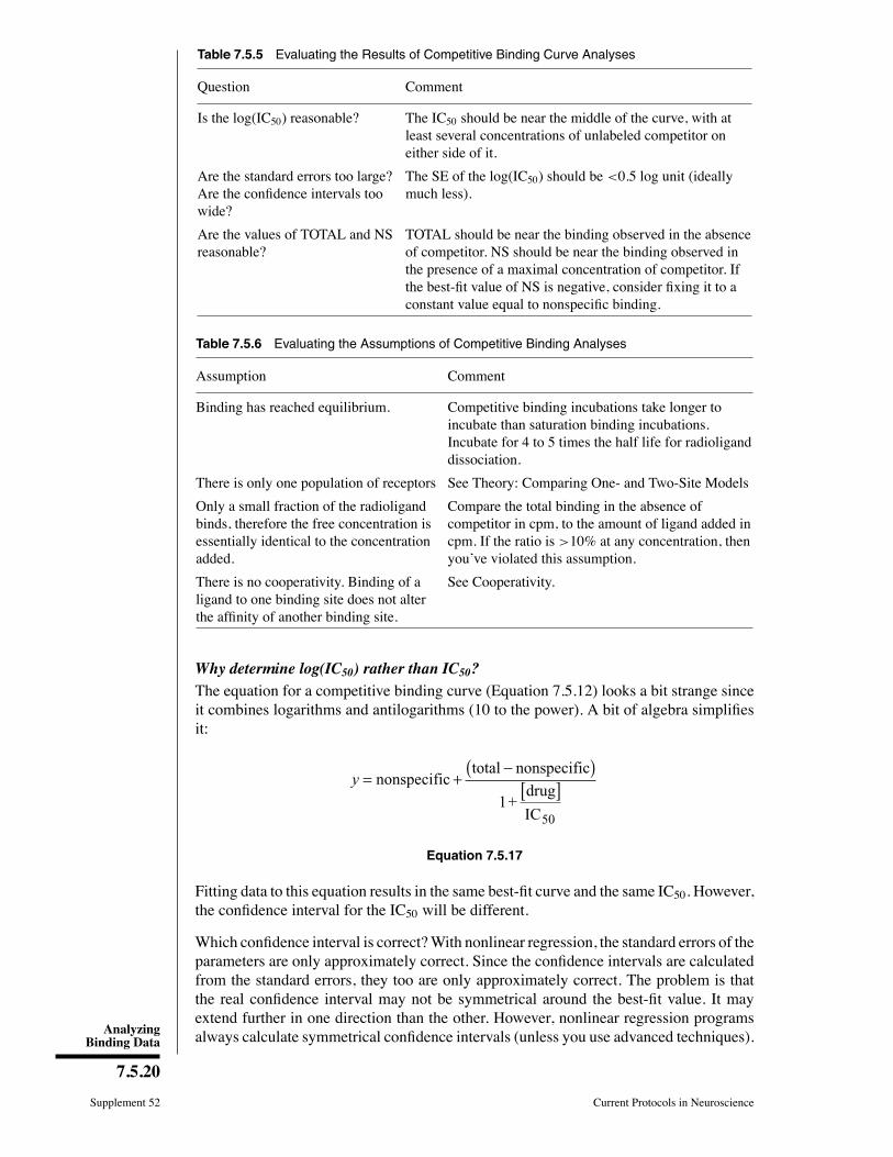
Table 7.5.5 Evaluating the Results of Competitive Binding Curve Analyses
Question Comment
Is the log(IC50) reasonable? The IC50 should be near the middle of the curve, with atleast several concentrations of unlabeled competitor oneither side of it.
Are the standard errors too large?Are the conÞdence intervals toowide?
The SE of the log(IC50) should be <0.5 log unit (ideallymuch less).
Are the values of TOTAL and NSreasonable?
TOTAL should be near the binding observed in the absenceof competitor. NS should be near the binding observed inthe presence of a maximal concentration of competitor. Ifthe best-Þt value of NS is negative, consider Þxing it to aconstant value equal to nonspeciÞc binding.
Table 7.5.6 Evaluating the Assumptions of Competitive Binding Analyses
Assumption Comment
Binding has reached equilibrium. Competitive binding incubations take longer toincubate than saturation binding incubations.Incubate for 4 to 5 times the half life for radioliganddissociation.
There is only one population of receptors See Theory: Comparing One- and Two-Site Models
Only a small fraction of the radioligandbinds, therefore the free concentration isessentially identical to the concentrationadded.
Compare the total binding in the absence ofcompetitor in cpm, to the amount of ligand added incpm. If the ratio is >10% at any concentration, thenyou�ve violated this assumption.
There is no cooperativity. Binding of aligand to one binding site does not alterthe afÞnity of another binding site.
See Cooperativity.
Why determine log(IC50) rather than IC50?
The equation for a competitive binding curve (Equation 7.5.12) looks a bit strange sinceit combines logarithms and antilogarithms (10 to the power). A bit of algebra simpliÞesit:
y = +−( )
[ ]nonspecifictotal nonspecific
1+drug
IC50
Equation 7.5.17
Fitting data to this equation results in the same best-Þt curve and the same IC50. However,the conÞdence interval for the IC50 will be different.
Which conÞdence interval is correct?With nonlinear regression, the standard errors of theparameters are only approximately correct. Since the conÞdence intervals are calculatedfrom the standard errors, they too are only approximately correct. The problem is thatthe real conÞdence interval may not be symmetrical around the best-Þt value. It mayextend further in one direction than the other. However, nonlinear regression programsalways calculate symmetrical conÞdence intervals (unless you use advanced techniques).

Neurochemistry/Neuropharma-cology
7.5.21
Current Protocols in Neuroscience Supplement 52
Log[yohimbine]
4000
5000
0
3000
0 –9
[3H
] U
K 1
4304 b
ound
(cpm
)
2000
1000
Log
[competitor](M)
−12.0
−10.0
−9.5
−9.0
−8.5
−8.0
Binding (cpm)
in triplicate
4549
4604
4353
4192
4053
3453
2587
1295
886
591
580
521
4380
4803
4278
4156
4420
3018
2946
1405
880
612
559
545
−7.5
−7.0
−6.5
−6.0
−5.5
−5.0
4554
4213
4508
3972
4191
3024
2367
1402
888
603
555
555
–7 –5–10 –8 –6
Figure 7.5.11 Example of a competitive binding experiment. Yohimbine competes for radioligand
binding to α2 receptors on membranes.
Therefore, when writing the equation for nonlinear regression, choose parameters so theuncertainty is as symmetrical as possible. Because data are collected at concentrationsof unlabeled drug equally spaced on a log axis, the uncertainty is symmetrical whenthe equation is written in terms of the log(IC50), but is not symmetrical when written interms of IC50. Thus, conÞdence intervals are more accurate when the equation is writtenin terms of the log(IC50).
Figure 7.5.11 (R. Neubig, unpub. observ.) shows competition of unlabeled yohimbinefor labeled UK14341 (an α2 adrenergic agonist).
1. Enter the data into a nonlinear regression program. Enter the logarithm of concentra-tion of the unlabeled ligand in the x column, and the triplicate values of total bindingin the x columns. If the selected program does not allow entry of triplicate values,enter each log of concentration three times.
2. Fit the data to a one-site competitive binding curve. If necessary, enter it in this format:
yx
= + −+
⎡
⎣⎢⎢
⎤
⎦⎥⎥−( )NS Total
NS
IC1 10 50log
Equation 7.5.18
3. If the nonlinear regression program does not provide initial values automatically,estimate the values of the parameters. TOTAL is the top plateau of the curve, soestimate its value from the highest data values, perhaps 4500. NS is the bottomplateau, so estimate its value from the lowest data values, perhaps 500. Log(IC50) isthe x value in the middle of the curve. From looking at the data, estimate its value as−7. None of these estimates has to be very accurate, and the nonlinear regression willprobably work Þne even if the estimates are fairly different than the values listed here.
4. Note the best-Þt results: NS = 530.3, TOTAL = 4418, and log(IC50) = −7.532.5. Convert the log(IC50) to the IC50 by taking the antilog. IC50 = 29.4 nM.

AnalyzingBinding Data
7.5.22
Supplement 52 Current Protocols in Neuroscience
6. Convert the IC50 to Ki. To do this, the concentration of radioligand used (2.0 nM)and its Kd for the receptors (0.88 nM, determined in a separate saturation bindingexperiment not shown here) must be known:
K
K
i
d
IC
1+radioligand
nM
nM
nM
nM= [ ] =+
=50 29
12 0
0 88
8 98.4
.
.
.
Equation 7.5.19
Homologous Competitive Binding Curves
A competitive binding experiment is termed homologous when the same compound isused as the hot and cold ligand. The term heterologous is used when the hot and coldligands differ. Homologous competitive binding experiments can be used to determinethe afÞnity of a ligand for the receptor and the receptor number. In other words, theexperiment has the same goals as a saturation binding curve. Because homologouscompetitive binding experiments use only one or two concentrations of radioligand(which can be low), they consume less radioligand and thus are more practical thansaturation experiments when radioligands are expensive or difÞcult to synthesize.
Analyses of homologous competitive binding curves depend on the following assump-tions:
1. The receptor has identical afÞnity for the labeled and unlabeled ligand. If you choose aniodinated radioligand, you should also use an iodinated unlabeled compound (usingnonradioactive iodine), because iodination often changes the binding properties ofligands.
2. There is no cooperativity.
3. There is no ligand depletion. The methods in this section assume that only a smallfraction of ligand binds. In other words, the method assumes that free concentrationequals the concentration added.
4. There is only one class of binding sites. It is difÞcult to detect a second class ofbinding sites unless the number of lower-afÞnity sites vastly exceeds the number ofhigher-afÞnity receptors (because the single low concentration of radioligand used inthe experiment will bind to only a small fraction of low afÞnity receptors).
Homologous competition follows this model, where Bmax is the total number of bindingsites (in the same units as y), H is the concentration of radioligand (hot), C is theconcentration of unlabeled (cold) ligand, Kd is the dissociation constant you are tryingto determine, and NS × H is the amount of nonspeciÞc binding in the same units as y.H, C, and Kd must all be expressed in the same concentration units. Note that Bmax is thetotal number of binding sites, which exceeds the number bound by radioligand in thisexperiment.
yB H
H C KH= −
+ ++ ⋅max
d
NS
Equation 7.5.20
To get reliable data, it is best to use two different concentrations of radioligand, and Þtthe two curves globally�sharing the values of Bmax, Kd, and NS so that there is only one

Neurochemistry/Neuropharma-cology
7.5.23
Current Protocols in Neuroscience Supplement 52
Log[Yomimbine] (M)10-100 10-9 10-8 10-7 10-6
hot = 5 nM
Tota
l bin
din
g (
cpm
)
hot = 2 nM
15,000
5000
000
10,000,,
Figure 7.5.12 Example of homologous competitive binding experiment. The hot and cold ligands
are identical.
best-Þt value for the entire experiment. Note that the amount of nonspeciÞc binding isthe product of the concentration of hot ligand, H, and the parameter NS. That product isdifferent for each concentration of ligand, even though NS is shared:
B
K
max = − = −[ ]+ [ ]( )
TOP BOTTOM
fractional occupancy
TOP BOTTOM
radioligand
radioligandd
Equation 7.5.21
Example of homologous competitive binding
Figure 7.5.12 shows data from a binding experiment using [3H]yohimbine to quantify α2adrenergic receptors to compete with unlabeled yohimbine. There is no reason to thinkthat adding a tritium label will alter yohimbine�s afÞnity for the receptor, so it seems safeto assume that hot and cold yohimbine bind with the same afÞnity.
1. Enter the data into a nonlinear regression program. Enter the logarithm of concentra-tion as x and cpm bound as y. The Þrst point represents a control with no yohimbine.Since the log of zero is undeÞned, this cannot be shown on a log scale. Instead enterthis value as −12 (the exact value is a bit arbitrary but any value much smaller thanthe Kd will work.).
2. Fit the data using global nonlinear regression to this equation, sharing all three pa-rameters and setting HotnM to a different constant value for each data set.
ColdNM=10ˆ (x+9); Cold concentration in nMKdNM=10ˆ (logKD+9); Kd in nMBottom=NS*HotnMY=(Bmax*HotnM)/(HotnM + ColdNM + KdNM) + Bottom
The Þrst line converts the x values in log(molar) to concentrations in nM.
The next line converts the log of Kd (which the program will Þt) to the Kd in nM.
The third line calculates the bottom plateau of the curve.
The Þnal line matches Equation 7.5.20.
If you don�t have access to a program that can do global nonlinear regression, Þt eachdata set individually.

AnalyzingBinding Data
7.5.24
Supplement 52 Current Protocols in Neuroscience
Table 7.5.7 Fitted Parameters Determined from Data in Figure 7.5.12
Parameter Global Þt Only Þt 5 nM data Only Þt 2 nM data
Best Þt 95% CI Best Þt 95% CI Best Þt 95% CI
Bmax (cpm) 11753 8812 to 14734 6820 4353 to 9286
Log Kd −8.67 −8.93 to −8.41 Did not converge −9.28 −10.02 to−8.545Kd (nM) 2.14 1.19 to 3.87 0.54 0.009 to 2.84
Pe
rce
nt
sp
ecific
bin
din
g
−3
100
50
0
Log[unlabeled competitor]
−4−5−6−7−8−9
slope = −1.00slope = −0.75slope = −0.50
Figure 7.5.13 Examples of slope factors. The slope factor quantifies the steepness of the curve,
and is determined by nonlinear regression of competitive binding data. It is not the same as the
slope of the curves at the midpoints.
3. The best-Þt results are shown in Table 7.5.7.
It was not possible to Þt the 5 nM data. The Þt simply did not converge. The data donot deÞne unique values for the Bmax and Kd. It was possible to Þt the 2 nM data, butthe Kd was poorly determined with wide conÞdence interval. The global Þt workedmuch better, giving useful results.
4. Finally convert Bmax to more useful units. In this example there were 6 × 10⁴
cells per well, the speciÞc activity of the [3H]yohimbine was 78 Ci/mmol, andthe scintillation counting efÞciency was 33%. Calculate receptors/cell using theequation:
11,753 cpm receptors/mmol
dpm/Ci cpm/
× ×× ×
6 02 10
2 22 10 0 33
20
12
.
. . ddpm Ci/mmol 60,000 cellsreceptors/cell
× ×= ×
782 06 106.
Equation 7.5.22
The Slope Factor or Hill Slope
Many competitive binding curves are shallower than predicted by the law of mass actionfor binding to a single site. The steepness of a binding curve can be quantiÞed with aslope factor, often called a Hill slope. A one-site competitive binding curve that followsthe law of mass action has a slope of−1.0. If the curve is shallower, the slope factor willbe a negative fraction (i.e.,−0.85 or−0.60; see Fig. 7.5.13). The slope factor is negativebecause the curve goes downhill.

Neurochemistry/Neuropharma-cology
7.5.25
Current Protocols in Neuroscience Supplement 52
To quantify the steepness of a competitive binding curve (or a dose-response curve), Þtthe data to this equation:
( )( )50log IC log slope factor
total NStotal radioligand binding NS
1 10x− ×
−= +
+
Equation 7.5.23
The slope factor is a number that describes the steepness of the curve. In most situations,there is no way to interpret the value in terms of chemistry or biology. If the slope factordiffers signiÞcantly from −1.0, then the binding does not follow the law of mass actionwith a single site.
Explanations for shallow binding curves include:
1. Heterogeneous receptors. Not all receptors bind the unlabeled drug with the sameafÞnity. This can be due to the presence of different receptor subtypes, or due toheterogeneity in receptor coupling to other molecules such as G proteins. InFig. 7.5.13, the slope factor equals −0.78.
2. Negative cooperativity. Binding sites are clustered (perhaps several binding sites permolecule) and binding of the unlabeled ligand to one site causes the remaining site(s)to bind the unlabeled ligand with lower afÞnity.
3. Curve Þtting problems. If the top and bottom plateaus are not correct, then the slopefactor is not meaningful. Don�t try to interpret the slope factor unless the curve hasclear top and bottom plateaus.
KINETIC BINDING EXPERIMENTS
Dissociation Experiments
A dissociation binding experiment measures the �off rate� of radioligand dissociatingfrom the receptor. Performdissociation experiments to fully characterize the interaction ofligand and receptor and conÞrm that the lawofmass action applies. Such experimentsmayalso be used to help design the experimental protocol. If the dissociation is fast, Þlter andwash the samples quickly so that negligible dissociation occurs. Lowering the temperatureof the buffer used to wash the Þlters, or switching to a centrifugation or dialysis assay,may also be required. If the dissociation is slow, then the samples can be Þltered at amore leisurely pace, because the dissociation will be negligible during the wash.
To perform a dissociation experiment, Þrst allow ligand and receptor to bind, perhaps toequilibrium. At that point, block further binding of radioligand to receptor using one ofthese methods:
1. If the tissue is attached to a surface, remove the buffer containing radioligand andreplace with fresh buffer without radioligand.
2. Centrifuge the suspension, decant supernatant, and resuspend pellet in fresh buffer.
3. Add a very high concentration of an unlabeled ligand (perhaps 100 times its Ki forthat receptor). It will instantly bind to nearly all the unoccupied receptors and blockbinding of the radioligand.
4. Dilute the incubation by a large factor, perhaps a 20- to 100-fold dilution. This willreduce the concentration of radioligand by that factor. At such a low concentration,new binding of radioligand will be negligible. This method is only practical when

AnalyzingBinding Data
7.5.26
Supplement 52 Current Protocols in Neuroscience
using a fairly low radioligand concentration so its concentration after dilution is farbelow its Kd for binding.
After initiating dissociation,measure binding over time (typically 10 to 20measurements)to determine how rapidly the ligand dissociates from the receptors.
Using nonlinear regression to determine koff1. Enter the x data as time in minutes.
2. Enter the y data as total binding in cpm.
3. Choose the exponential dissociation equation. Total binding and nonspeciÞc binding(NS) are expressed in cpm, fmol/mg protein, or sites/cell. Time (t) is usually expressedin minutes. The dissociation rate constant (koff) is expressed in units of inverse time,usually min−1:
total binding NS total NS off= + −( ) × −e k t
Equation 7.5.24
4. If the chosen nonlinear regression program does not provide initial estimates of theparameters, enter these values. Total is the total binding at time zero and is estimatedas the Þrst y value. NS is the binding after a long time, and reßects nonspeciÞc binding.Estimate it as the last y value. K is the dissociation rate constant (koff). Estimate it bydividing 0.69 by an estimate of the half-time of dissociation.
5. Start the nonlinear regression procedure.
6. Calculate the half-life of dissociation from the rate constant.
half-life l off= ( ) =n .2 0 693k K
Equation 7.5.25
In one half-life, half the radioligand will have dissociated (see Fig. 7.5.14). In twohalf-lives, three quarters of the radioligand will have dissociated, etc.
Typically the dissociation rate constant of useful radioligands is between 0.001 and0.1 min−1. If the dissociation rate constant is any faster, it will be difÞcult to performradioligand binding experiments, as the radioligand will dissociate from the receptors
total
NS
Timet1/2
Tota
l bin
din
g
Figure 7.5.14 Schematic of a dissociation kinetic experiment.

Neurochemistry/Neuropharma-cology
7.5.27
Current Protocols in Neuroscience Supplement 52
Ln(s
pecific
bin
din
g)
slope = −koff
Time
Figure 7.5.15 Schematic of a dissociation kinetic experiment shown on a log scale. The y axis
plots the natural log of specific binding.
while you wash the Þlters. If the dissociation rate constant is any slower, it will be hardto reach equilibrium.
Displaying dissociation data on a log plot
Figure 7.5.15 shows a plot of ln(Bt/B0) versus time. The graph of a dissociation experimentwill be linear if the system follows the law of mass action with a single afÞnity state. Btis the speciÞc binding at time t; B0 is speciÞc binding at time zero. The slope of this linewill equal −koff.The log plot will only be linear when taking the logarithm of speciÞc binding as a fractionof binding at time zero. Don�t use total binding.
Use the natural logarithm, not the base ten log in order for the slope to equal −koff. Ifyou use the base 10 log, then the slope will equal −2.303 times koff.Use the log plot only to display data, not to analyze data. A more accurate rate constantwill be obtained by Þtting the raw data using nonlinear regression.
Association Binding Experiments
Association binding experiments are used to determine the association rate constant.This value is useful to characterize the interaction of the ligand with the receptor. It isalso important as it permits the determination of the time it takes to reach equilibrium insaturation and competition experiments.
To perform an association experiment, add a single concentration of radioligand andmeasure speciÞc binding at various times thereafter. You can also do the experiment withseveral different concentrations of radioligand.
Association of ligand to receptors (according to the law of mass action) follows theequation:
specific binding max ob= × −( )− ×1 e k t
Equation 7.5.26
In Figure 7.5.16, note that the maximum binding (max) is not the same as Bmax. Themaximum (equilibrium) binding achieved in an association experiment depends on theconcentration of radioligand. Low to moderate concentrations of radioligand will bind

AnalyzingBinding Data
7.5.28
Supplement 52 Current Protocols in Neuroscience
max
TimeS
pe
cific
bin
din
g
Figure 7.5.16 Schematic of an association kinetic experiment.
to only a small fraction of all the receptors no matter how long binding is allowed toproceed.
Note that the equation used for Þtting does not include the association rate constant,kon, but rather contains the observed rate constant, kob, which is expressed in units ofinverse time (usually min−1). The kob is a measure of how quickly the incubation reachesequilibrium and in the case of a simple bimolecular binding reaction is deÞned by thisequation:
k k kob off on radioligand= + ×[ ]
Equation 7.5.27
The equation deÞnes kob as a function of three factors:
1. The association rate constant, kon. This is what is to be determined. If kon is larger(faster), kob will be larger as well.
2. The concentration of radioligand. When using more radioligand, the system willequilibrate faster and kob will be larger.
3. The dissociation rate constant, koff. It may be surprising to discover that the observedrate of association depends in part on the dissociation rate constant. This makes sensebecause an association experiment does not directly measure how long it takes radioli-gand to bind, but rather measures how long it takes the binding to reach equilibrium.Equilibrium is reached when the rate of the forward binding reaction equals the rateof the reverse dissociation reaction. If the radioligand dissociates quickly from thereceptor, equilibrium will be reached faster, but there will be less binding at equilib-rium. If the radioligand dissociates slowly, equilibrium will be reached more slowlyand there will be more binding at equilibrium.
To calculate the association rate constant, usually expressed in units of M−1 min−1, usethe following equation. Typically ligands have association rate constants of ∼108 M−1min−1.
kk k
onob off
radioligand= −
[ ]
Equation 7.5.28

Neurochemistry/Neuropharma-cology
7.5.29
Current Protocols in Neuroscience Supplement 52
Determining konwhen you already know koff1. Enter the x data as time in minutes.
2. Enter the y data as total binding in cpm.
3. Fit to this equation, constraining koff to a constant value based on other experimentsand HotnM to the concentration of radioligand in nM.
Kd=koff/konL=Hotnm*1e-9kob=kon*L+koffOccupancy=L/(L+Kd)Ymax=Occupancy*BmaxY=Ymax*(1 - exp(-1*kob*X)) + NS
4. Provide the nonlinear regression program with initial estimates of the parameters.Bmax is the maximum speciÞc binding at equilibrium with high ligand concentration,expressed in the same units as Y, so it can be estimated as 2 to 5 times the last y value.NS is the nonspeciÞc binding in the same units as y, so is estimated by the smallest yvalue. kon is the association rate constant. There is no straightforward rule to use forits initial value, so use a standard value of 1E8 (the units are min−1 M−1).
5. Start the nonlinear regression procedure to determine kon, NS, and Bmax. Note thatKd, L, kob, Occupancy, and Ymax are all intermediate variables used to make theequation more clear. Their value is computed from the two constants (hotnm and koff)and the two parameters you are Þtting (kon and Bmax).
Determining kon and koff in one experiment
After running an association experiment, add cold ligand to initiate dissociation. Thislets you Þt both the association and dissociation rate constants in one experiment.
1. Enter the x data as time in min.
2. Enter the y data as total binding in cpm.
3. Fit to this equation, constraining HotnM to the concentration of radioligand in nMand Time0 to the time at which dissociation was initiated.
Radioligand=HotNM*1e-9kob=[Radioligand]*kon+koffKd=koff/konEq=Bmax*radioligand/(radioligand + Kd)Association=Eq*(1-exp(-1*kob*X))YatTime0 = Eq*(1-exp(-1*kob*Time0))Dissociation= YatTime0*exp(-1*koff*(X-Time0))Y=IF(X<Time0, Association, Dissociation) + NS
4. Provide the nonlinear regression program with initial estimates of the parameters.Bmax is the maximum speciÞc binding at equilibrium with high ligand concentration,expressed in the same units as Y, so can be estimated as a few times the largest yvalue. kon is the association rate constant. There is no straightforward rule to use forits initial value, so use a standard value of 1E8 (the units are min−1 M−1).
5. Start the nonlinear regression procedure to determine kon, koff, and Bmax . Note thatKd, L, kob, Association, YatTime0, and Dissociation are all intermediatevariables used to make the equation more clear. Their value is computed from the twoconstants (hotnm and koff) and the two parameters you are Þtting (kon and Bmax).

AnalyzingBinding Data
7.5.30
Supplement 52 Current Protocols in Neuroscience
Table 7.5.8 Evaluating the Results of Association Binding Analyses
Question Comment
Were data collected over a longenough period of time?
Dissociation and association data should plateau, so thedata obtained at the last few time points should beindistinguishable.
Is the value of kon reasonable? The association rate constant, kon, depends largely ondiffusion, so the value is similar for many ligands. Expecta result of ∼108 M−1 min−1.
Is the value of koff reasonable? If the koff is >1 min−1, the ligand has a low afÞnity for thereceptor. Most likely, dissociation will occur duringseparation of bound and free ligands. If koff is <0.001min−1, attaining equilibrium will be difÞcult as thehalf-time of dissociation will be greater than 10 hr! Even ifone waits that long, other reactions may occur that ruin theexperiment.
Are the standard errors too large?Are the conÞdence intervals toowide?
Examine the SE and the conÞdence intervals to gauge thelevel of conÞdence to give the rate constants.
Does only a tiny fraction ofradioligand bind to the receptors?
The standard analyses of association experiments assumethat the concentration of free radioligand is constantduring the experiment. This will be approximately trueonly if a tiny fraction of the added radioligand binds to thereceptors. Compare the maximum total binding in cpm tothe amount of added radioligand in cpm. If that ratioexceeds ∼10%, revise the experimental protocol.
Interpreting Kinetic Results
Are the results reasonable?
Table 7.5.8 presents some questions that should be addressed when determining if theresults are reasonable.
Using Kinetic Data to Test the Law of Mass Action
Standard binding experiments are usually Þt to equations derived from the law of massaction. Kinetic experiments provide a more sensitive test than equilibrium experimentsto determine whether the law of mass action actually applies for the system of interest.To test the law of mass action, ask the following questions.
Does the Kd calculated from kinetic data match the Kd calculated from saturationbinding?
According to the law of mass action, the ratio of koff to kon is the Kd of receptor binding:
Kk
kdoff
on
=
Equation 7.5.29
The units are consistent: koff is in units of min−1 and kon is in units of M−1min−1, so Kd
is in units of M.
If binding follows the law of mass action, the Kd calculated in this way should be thesame as the Kd calculated from a saturation binding curve.

Neurochemistry/Neuropharma-cology
7.5.31
Current Protocols in Neuroscience Supplement 52
[Radioligand]
slope = kon
koff
Ko
b(m
in–
1)
Figure 7.5.17 Schematic of observed association rate constants as a function of radioligand
concentration. Higher concentrations of radioligand equilibrate more quickly. The slope of the line
equals the association rate constant (kon); the y intercept is the dissociation rate constant (koff).
Does kob increase linearly with the concentration of radioligand?
The observed association rate constant, kob, is deÞned by this equation:
k k kob off on radioligand= + × [ ]
Equation 7.5.30
Therefore, association rate experiments performed at various concentrations of radioli-gand should look like Figure 7.5.17. As the concentration of radioligand is increased, theobserved rate constant increases linearly. If the binding is more complex than a simplemass action model (such as a binding step followed by a conformational change), theplot of kob versus [radioligand] may plateau at higher radioligand concentrations. They intercept of the line equals koff. If the law of mass action applies to the system, thekoff determined in this way should correspond to the koff determined from a dissociationexperiment. Finally, this kind of experiment provides a more rigorous determination ofkon than the value obtained with a single concentration of radioligand.
Is speciÞc binding 100% reversible, and is the dissociated ligand chemically intact?
NonspeciÞc binding at �time zero� should equal total binding at the end (plateau) ofthe dissociation. In other words, all of the speciÞc binding should dissociate after asufÞciently long period of time. Use chromatography to analyze the radioligand thatdissociates to prove that it has not been altered.
Is the dissociation rate the same when dissociation is initiated from differentamounts or times of receptor occupation?
If the ligand binds to a single site and obeys the law of mass action, the dissociation rateconstant is independent of the amount of radioligand used or the time before initiatingdissociation.
Is there cooperativity?
If the law of mass action applies, binding of a ligand to one binding site does not alter theafÞnity of another binding site. This also means that dissociation of a ligand from onesite should not change the dissociation of ligand from other sites. To test this assumption,compare dissociation initiated by adding an unlabeled ligand with dissociation initiatedby inÞnite dilution. The two rate constants should be identical (see Competitive Bindingwith Two Sites, below).

AnalyzingBinding Data
7.5.32
Supplement 52 Current Protocols in Neuroscience
Kinetics of Competitive Binding
The standard methods of kinetic binding determine the kon and koff for a labeled ligand.Competitive binding can be used to determine the kon and koff of an unlabeled ligand.Add the two ligands at the same time, and measure radioligand binding over time. Usethe following information to set up the equation (Motulsky and Mahan, 1984).
DeÞne the following parameters:
k1 association rate constant of radioligand (M−1 min−1)k2 dissociation rate constant of radioligand (min−1)k3 association rate constant of unlabeled ligand (M−1 min−1)k4 dissociation rate constant of unlabeled ligand (min−1)[radioligand] concentration of labeled drug (M)[unlabeled drug] concentration of unlabeled drug (M)S an arbitrary designation of an intermediate variableBmax total number of binding sites (same units as speciÞc binding, usually cpm)t time (min)
K k kA radioligand= × [ ] +1 2
Equation 7.5.31
K k kB unlabeled ligand= × [ ] +3 4
Equation 7.5.32
S radioligand unlabeled ligandA B= −( ) + × × × [ ] × [ ]K K k k2
1 34
Equation 7.5.33
KK K
KK K
FA B
SA BS S= + + =
2 2
Equation 7.5.34
specific binding
radioligand
F S
F S
F S
F
F
S
S
F S
=
× × [ ]−
× −( )×
+ − × −−
×⎡
⎣⎢
⎤
⎦⎥− ⋅ − ⋅B k
K K
k K K
K K
k K
Ke
k K
KeK t K tmax 1 4 4 4
Equation 7.5.35
Many data points are needed at early time points for this method to work. When Þttingthe data, set k1 and k2 to constant values determined from standard kinetic experimentswith the radioligand. Set Bmax to a constant value determined in a saturation bindingexperiment. The concentrations of labeled and unlabeled compound are also constants,set by your experimental design. Fit the data to determine k3 and k4.
To get reliable results, perform the experiment with two concentrations of radioligand,and Þt both data sets globally, sharing all the parameters.

Neurochemistry/Neuropharma-cology
7.5.33
Current Protocols in Neuroscience Supplement 52
TWO BINDING SITES
Several receptor molecules frequently evolve for a single hormone or neurotransmitter.Also, many ligands bind to more than one receptor subtype. Consequently, it is oftennecessary to Þt binding data with a model that includes two or more binding sites.
Saturation Binding Experiments with Two Sites
When the radioligand binds to two classes of receptors, analyze the data by using thisequation:
specific bindingL
L
L
Ld d
= = × [ ]+ [ ]
+ × [ ]+ [ ]
yB
K
B
Kmax max1
1
2
2
Equation 7.5.36
Panel A of Figure 7.5.18 shows speciÞc binding to two classes of receptors present inequal quantities, whose Kd values differ by a factor of ten. Panel B shows the transfor-mation to a Scatchard plot. In both graphs the dotted and dashed lines show binding tothe two individual receptors; the sum in each graph is represented by a solid curve.
0 50 100 150 200
0
25
50
75
Bo
un
d/f
ree
Specific binding
0 25 50 75 100
0
100
200
Sp
ecific
bin
din
g
[Radioligand]
A
B
Figure 7.5.18 Saturation binding to two classes of receptors. The two receptor types are present
in equal quantities, but have Kd values that differ by a factor of ten. (A) Binding to the two individual
receptor types are shown as dashed curves. The sum (observed experimentally) is shown as
a solid curve. It is not obviously biphasic. (B) Scatchard transformation. The curvature of the
overall Scatchard plot (solid) is subtle, and it would be easy to miss the curvature if the data were
scattered. Note that the Scatchard plots for the individual receptors (dashed) are not asymptotes
of the two-site Scatchard plot (solid).

AnalyzingBinding Data
7.5.34
Supplement 52 Current Protocols in Neuroscience
Note that the graph of speciÞc binding is not obviously biphasic. It is very hard to see thepresence of two binding afÞnities by just looking. The best way to detect the second site isto Þt data to one- and two-site curves, and let the nonlinear regression program comparethe two Þts (see Theory: Comparing One- and Two-Site Models, below). The curvatureof the Scatchard plot is not dramatic and can easily be obscured by experimental scatter.Note the location of the solid and dashed line in the Scatchard plot. The two componentsof a biphasic Scatchard are not the asymptotes of the curve.
Competitive Binding with Two Sites
Competitive binding experiments are often used in systems where the tissue containstwo classes of binding sites (e.g., two subtypes of a receptor). Analysis of these data isstraightforward if the following assumptions are met:
1. There are two distinct classes of receptors. For example, a tissue could contain amixture of β1 and β2 adrenergic receptors.
2. The unlabeled ligand has distinct afÞnities for the two sites.
3. The labeled ligand has equal afÞnity for both sites or the afÞnity of the radiologicalfor the two sites is known from other experiments.
4. Binding has reached equilibrium.
5. A small fraction of both labeled and unlabeled ligand bind. This means that the con-centration of labeled and unlabeled ligand added is very close to the free concentrationin all tubes.
Based on these assumptions, binding follows the equation:
( ) ( ) ( )50 50log log IC A log log IC B
1NS Total NS
1 10 1 10x x
F Fy
− −
−⎡ ⎤= + − +⎢ ⎥+ +⎣ ⎦
Equation 7.5.37
This equation has Þve parameters: the total and nonspeciÞc binding (the top and bottombinding plateaus), the fraction of binding to receptors of the Þrst type of receptor (F), andthe IC50 of the unlabeled ligand for each type of receptor. If the Kd and concentration ofthe labeled ligand is known, the IC50 values can be converted to Ki values (see AnalyzingCompetitive Binding Data, above).
Since there are two different kinds of receptors with different afÞnities, a biphasiccompetitive binding curve might be expected. In fact, a biphasic curve is seen only inunusual caseswhere the afÞnities are extremely different.More often, the two componentsare blurred together into a shallow curve. For example, Figure 7.5.19 shows competitionfor two equally abundant sites with a ten-fold (one log unit) difference in IC50. Carefulobservation will reveal that the curve is shallow (it takes more than two log units to gofrom 90% to 10% competition), but two distinct components are not visible.
Cooperativity
In the standard mass action model, each binding site is independent. The standard massaction model assumes that there is no cooperativity. Cooperativity occurs when bindingof a ligand to one binding site affects binding to adjacent sites. Usually these binding sitesare on the same molecule. If binding of one ligand increases the afÞnity of an adjacentsite, this is positive cooperativity. This results in a Hill slope with an absolute valuegreater than 1. If binding of one ligand decreases the afÞnity of an adjacent site, this is

Neurochemistry/Neuropharma-cology
7.5.35
Current Protocols in Neuroscience Supplement 52
Log[unlabeled competitor]
IC50 site BSp
ecific
bin
din
g
IC50 site A
Figure 7.5.19 Two-site competitive binding curve. The radioligand binds identically to two kinds
of receptors, but these two receptors have a ten-fold difference in affinity for the competitor. The
curve is shallow, but not obviously biphasic.
negative cooperativity. This results in a Hill slope with an absolute value less than 1. Itis impossible to distinguish negative cooperativity from multiple independent bindingsites (with different afÞnities) from data collected at equilibrium. Kinetic experimentsare needed.
To distinguish between multiple independent binding sites and negative cooperativity,compare the dissociation rate after initiating dissociation by inÞnite dilution with thedissociation rate when initiated by addition of a large concentration of unlabeled drug.If the radioligand is bound to multiple noninteracting binding sites, the dissociationwill be identical in both experimental protocols as shown in panel A of Figure 7.5.20.Note that the y axis is shown using a log scale. If there were a single binding site, thedissociation data would be expected to appear linear on this graph. With two bindingsites, the graph is curved, even on a log axis (assuming the radioligand is present at highenough concentration to bind appreciably to both sites).
Panel B shows ideal dissociation data when radioligand is bound to interacting bindingsites with negative cooperativity. The data are different depending on how dissociationwas initiated. If dissociation is initiated by inÞnite dilution, the dissociation rate willchange over time. The dissociation of some radioligand will leave the remaining ligandbound more tightly. When dissociation is initiated by addition of cold drug, all thereceptors are always occupied by ligand (some hot, some cold) and dissociation occursat its maximal unchanging rate.
Theory: Comparing One- and Two-Site Models
Why not just compare sum of squares or R2?
In a least-squares analysis of data (either linear or nonlinear), the computer program willgive an R2 value and the sum of the squared deviations from the theoretical Þt in theexperimental result. The smaller the sum of squares (SS) value and the higher the R2, thebetter the theory Þts the data. However, a two-site model will almost always Þt the databetter than a one-site model. A three-site model Þts even better, and a four-site modelbetter yet! As more parameters (sites) are added to the equation, more inßection pointsare added to the curve, so it gets closer to the points. The sum of squares gets smallerand R2 gets higher. Statistical calculations (such as the F test described below) should beused to see whether these changes are larger than expected by chance.

AnalyzingBinding Data
7.5.36
Supplement 52 Current Protocols in Neuroscience
Bt/B
0
0.01
0.10
1.00
Bt/B
0
0.01
0.10
1.00
Time
infinite dilution
excess unlabeled
A
B
Figure 7.5.20 Discriminating between binding to two (or more) binding sites (A) and negative
cooperativity (B). With negative cooperativity, dissociation will be faster when initiated by adding
excess unlabeled ligand than when initiated by infinite dilution.
Reality check
Before performing statistical comparisons, however, look at whether the results makesense. Sometimes the two-site Þt gives results that are clearly nonsense. Disregard atwo-site Þt when:
1. The two IC50 or Kd values are almost identical�the data probably Þt quite well by asingle-site model.
2. One of the IC50 or Kd values is outside the range of data.
3. One of the sites has a very small fraction of the receptors �if there are too few sites,the IC50 or Kd cannot be determined reliably.
4. The best-Þt values for the bottom and top plateaus are far from the range of y valuesobserved in the experiment (applies to competitive binding curves only).
If the two-site Þt seems reasonable, test whether the difference between the one- andtwo-site Þt is statistically signiÞcant.
Using the F test to compare one- and two-site Þts
Even if the simpler one-site model is correct, the Þt is expected to be worse (have thehigher sum of squares) because it has fewer inßection points (more degrees of freedom;DF). In fact, statisticians have proven that the relative increase in the sum of squaresis expected to equal the relative increase in degrees of freedom. In other words, if theone-site model is correct it would be expected that:
SS SS SS DF DF DF1 2 2 1 2 2−( ) ≈ −( )
Equation 7.5.38

Neurochemistry/Neuropharma-cology
7.5.37
Current Protocols in Neuroscience Supplement 52
If the more complicated two-site model is correct, then the relative increase in sumof squares (going from two-site to one-site) is expected to be greater than the relativeincrease in degrees of freedom:
SS SS SS DF DF DF1 2 2 1 2 2−( ) > −( )
Equation 7.5.39
Follow these steps to compare the two models:
1. Fit the data to the simpler (one-site) model and record the sum of squares (SS1) anddegrees of freedom (DF1). Degrees of freedom equal the number of data points minusthe number of Þtted parameters.
2. Fit the data to the more complicated (two-site) model and record the sum of squares(SS2) and degrees of freedom (DF2).
3. Look at whether the two-site model makes sense. If the best-Þt values don�t makesense (or the values for the two sites are almost the same), then discard the two-sitemodel and accept the one-site model.
4. Compare SS2 with SS1. If for some reason SS2 is larger than SS1, then the two-siteÞt is worse than the one-site Þt and should be discarded. Accept the one-site Þt. Inmost cases SS1 is larger, and further calculations will be needed.
5. Calculate the F ratio, which quantiÞes the relationship between the relative increasein sum of squares and the relative increase in degrees of freedom.
F = −( )−( )
SS SS SS
DF DF DF
1 2 2
1 2 2
Equation 7.5.40
The equation for calculating F is usually presented in this equivalent form (seeTable 7.5.9 for corresponding ANOVA table).
F = −( ) −( ) = −( ) =SS SS DF DF
SS DFDF DF DF DF DFn
1 2 1 2
2 21 2 2, d
Equation 7.5.41
Table 7.5.9 ANOVA Table for Comparison of One- and Two-Site Fitsa
Source of variation Sum of squares DF Mean square
Difference SS1 - SS2 DF1 - DF2 SSI - SS2
DF1 - DF2
Model 2 (complicated) SS2 DF2 SS2/DF2
Model 1 (simple) SS1 DF1aANOVA, analysis of variance.

AnalyzingBinding Data
7.5.38
Supplement 52 Current Protocols in Neuroscience
6. Use a table or program to determine the P value. When doing so, degrees of freedomshould be entered for both the numerator (DFn) and denominator (DFd). The numeratorhas (DF1− DF2) degrees of freedom. The denominator has DF2 degrees of freedom.
If the one-site model is correct, an F ratio near one and a large P value are expected. Ifthe two-site Þt is correct, a large F ratio and a small P value would be seen. The P valuecan be small for two reasons. One possibility is that the two-site model is correct. Theother possibility is that the one-site model is correct, but random scatter led the two-sitemodel to Þt better by chance. The P value tells how rarely this coincidence would occur.More precisely, the P value answers the following question: if the one-site model isreally correct, what is the chance that data would randomly Þt the two-site model somuch better?
If the P value is smaller than a preset threshold (set to the arbitrary value of 0.05 bytradition), conclude that the two-site model is signiÞcantly better than the one-site model.
Figure 7.5.21 compares a one-site and two-site competitive binding curve. The resultsare shown in Table 7.5.10.
In going from the two-site to the one-site model, two degrees of freedom are gained,because the one-site model has two fewer parameters. Since the two-site model has 10degrees of freedom (15 data points minus 5 parameters), the degrees of freedom increased20%. If the one-site model were correct, the sum of squares would be expected to increase∼20% just by chance. In fact, the sum of squares increased 91%. The percent increasewas 4.56 times higher than expected (91.1/20.0 = 4.56). This is the F ratio (F = 4.56),and it corresponds to a P value of 0.039. If the one-site model is correct, there is only a3.9% chance that randomly obtained data would Þt the two-site model so much better.Since this is below the traditional threshold of 5%, conclude that the two-site model ÞtssigniÞcantly better than the one-site model.
Table 7.5.10 Comparison of One-Site and Two-Site Competitive
Binding Curve
Two-site One-site % increase
Degrees of freedom 10 12 20.00
Sum of squares 129,800 248,100 91.14
Log[competitor]
Bin
din
g (
cpm
)
–10 –9 –8 –7 –6 –5 –4
0
1000
2000
3000
two sites
one site
Figure 7.5.21 The solid curve shows the fit to an equation describing competition for a single
class of receptors. The dashed curve shows the fit to an equation describing competition for
binding to two classes of receptors.

Neurochemistry/Neuropharma-cology
7.5.39
Current Protocols in Neuroscience Supplement 52
AGONIST BINDING
Receptors Linked to G Proteins
The most studied example of agonist binding is the interaction of agonists with receptorsthat are linked toGproteins. This is studied by comparing the competition of agonistswithradiolabeled antagonist binding in the presence and absence ofGTP (or its analogs). Theseexperiments are done in membrane preparations to wash away endogenous intracellularGTP. Without added GTP, the competitive binding curves tend to be shallow. When GTPor an analog is added, the competitive binding curve is of normal steepness. Figure 7.5.22shows the results of an idealized experiment.
The extended ternary complexmodel can partially account for these Þndings (and others).In this model, receptors can exist in two states, R and R*. The R* state has a high afÞnityfor agonist and preferentially associates with G proteins to form an R*G complex.Although some receptors may exist in the R* state in the absence of agonist, the bindingof agonist fosters the transition fromR toR*, and thus promotes interaction of the receptorwith G protein to form the ternary complex HR*G. The extended ternary complex modelis shown in Figure 7.5.23.
The agonist binding curve is shallow (showing high- and low-afÞnity components) inthe absence of GTP because some receptors interact with G proteins and others do not.
Log[agonist]
0
50
100
Perc
ent specific
bin
din
g
–GTP
+GTP
Figure 7.5.22 Schematic of agonist competition for binding to a receptor linked to a G protein. In
the absence of GTP (left) the curve is shallow (and in this extreme case, biphasic). In the presence
of GTP (or an analog) the curve is shifted to the right and is steeper.
H+R*+G HR*+G
H+R+G HR+G
H+R*G HR*G
H+R+G HR+G
H+RG HRG
H+R+G HR+G
H+RG HRG
Simple model Ternary complex model Extended ternary
complex model
Figure 7.5.23 Models for agonist binding to receptors linked to G proteins. H, hormone or agonist;
R, receptor; G, G protein.

AnalyzingBinding Data
7.5.40
Supplement 52 Current Protocols in Neuroscience
The receptors that do interact with G proteins bind agonist with high afÞnity, whilethose that do not interact bind with low afÞnity. Not all receptors can bind to G proteinsbecause either the receptors are heterogeneous, the G proteins are limiting, or membranecompartmentalization prevents some receptors from interacting with G proteins. If allthe receptors could interact with G proteins, the expectation would be a high afÞnity,competitive binding curve in the absence of GTP. In the presence of GTP (or an analog),the HR*G complex is not stable, so the G protein dissociates into its αGTP and βγ
subunits, and is uncoupled from the receptor. With GTP present, only a tiny fraction ofreceptors are coupled to G at any given time, so the agonist competition curves are oflow afÞnity and normal steepness as if only R was present and not RG.
Although the extended ternary complex model is very useful conceptually, it is not veryuseful when analyzing data. There are simply too many parameters. The simpler ternarycomplexmodel shown in Figure 7.5.23 has fewer parameters, but still toomany to reliablyÞt with nonlinear regression. For routine analyses, most investigators Þt data to the muchsimpler two-state model shown in the Þgure. This model allows for receptors to exist intwo afÞnity states (R and RG), but does not allow conversion between them. It is easy toÞt data to this simpler model using a two-site competition curve model. Since the modelis too simple, the high- and low-afÞnity dissociation constants derived from the modelshould be treated merely as empirical descriptions of the data and should not be thoughtof as true molecular equilibrium constants.
Other Kinds of Receptors
By deÞnition, the binding of agonists to receptors makes something happen. So it isnot surprising that agonist binding is often more complicated than the simple massaction model. For example, binding of agonists to nicotinic acetylcholine receptor causesa conformational change characterized by a high-afÞnity binding of the agonist anddesensitized receptors, and insulin binding to its receptor shows negative cooperativitydue to dimerization of the receptors.
USE OF FLUORESCENCE OR OTHER SPECTROSCOPIC METHODS INBINDING EXPERIMENTS
Advantages of Fluorescent Ligands
Recently, many investigators have begun to use nonradioactive methods to detect ligandbinding to receptors or macromolecules. In most cases, these methods use ßuorescentligands.
An advantage of ßuorescent methods is elimination of both the dangers of radioactivityand the expenses of radioactive waste disposal. Additionally, ßuorescent methods areeasier to perform and automate�a big plus for high throughput screening studies by thepharmaceutical industry. Fluorescent studies work very well for kinetics, since bindingin a single sample can be measured at many time points.
Disadvantages of Fluorescent Ligands
One disadvantage (compared to radioligands) is that ßuorescence measurements areexpressed in arbitrary ßuorescence units.While one can compare values between samplesin a single experiment, it is rarely possible to convert the ßuorescent measurements intothe actual number of binding sites in the incubation. This problem, however, does notaffect determinations of equilibrium or kinetic constants.
Another disadvantage of ßuorescent methods is that the signal-to-noise ratio tends to below.

Neurochemistry/Neuropharma-cology
7.5.41
Current Protocols in Neuroscience Supplement 52
Fluorescence methods rarely use a washing step to reduce nonspeciÞc binding (as radi-oligand methods do). Instead, ßuorescence is measured in the experimental incubation.The background signal includes not only binding to nonspeciÞc sites but primarilyßuorescence from the free ligand. The signal-to-noise problem is reduced when the con-centration of binding sites is high, as found in studies of puriÞed proteins or cell linesgenetically engineered to overexpress binding sites, and these are the kinds of systemswhere ßuorescence methods are most useful.
In order to detect a change in ßuorescence on ligand binding without physical separation,a signiÞcant fraction of the ligand often needs to be bound. This means that analyses ofßuorescent binding need to account for ligand depletion, as discussed earlier.
How Fluorescence Binding Measurements Work
Fluorescent ligand binding studies measure some change in the spectral properties of aßuorescent ligand upon binding to the receptor. There are at least three different methodsused for ßuorescent ligand binding studies: ßuorescence intensity (FI), ßuorescencepolarization (FP), and ßuorescence resonance energy transfer (FRET). The methods ofanalysis are similar for FI and FRET but because FP measures a ratio of two differentlypolarized emission values, the analysis of FP results is signiÞcantly different (see below).
A less frequently used method is to use a ßuorescent receptor (either natural ßuorescencesuch as tryptophan or a labeled protein) and detect changes in the spectral properties ofthe receptor as the small molecule binds. Finally, some other approaches make use of achange in localization of the ßuorescent ligand upon binding which concentrates it in thevicinity of an excitation light source [e.g., total internal reßection ßuorescence (TIRF), orbead-based methods such as ßow cytometry protein interaction assay (FCPIA) (Romanet al., 2007)]. In some cases, standard separation methods like Þltration are used withßuorescence detection of a bound ligand, but thosemethods entail the same considerationsas standard radioligand methods, and will not be considered here.
Fluorescence Intensity
Fluorescent intensity changes when the ßuorophore moves to a different environmenton binding, for example moving from an aqueous environment for the free ligand to ahydrophobic protein surface for the bound ligand. As increasing amounts of a ßuorescentligand are added to a biological preparation containing a receptor or binding site, ßuores-cence is detected from both the free ligand L and the bound ligand LR. If the ßuorescenceof the bound ligand is higher (or lower) than the ßuorescence of the free ligand, then thesystem can be used to measure binding. In general, however, a signiÞcant fraction of theligand must be bound (e.g., 2% to 50%) in order to detect a clear signal in FI studies.Saturation binding experiments lead to results similar to those for a radioligand satura-tion study (see Fig. 7.5.24), in which there is a linear component due primarily to theßuorescence from the free ligand and a saturable component due to the receptor binding.
Depending on the concentration of the receptor binding sites (Rtot) relative to the Kd forthe binding interaction, this may follow either a simple hyperbolic binding isotherm:
Fractional occupancyligand
ligand d
=[ ]
[ ]+ K
Equation 7.5.42
or that for a saturation curve with ligand depletion. As a rule of thumb, if Rtot is < Kd/5then it is appropriate to use the simple saturation isotherm with a linear nonspeciÞc

AnalyzingBinding Data
7.5.42
Supplement 52 Current Protocols in Neuroscience
theoretical curve with free fluorescence
Flu
ore
scence
Bound li
gand (
nM
)B
ound li
gand (
% o
f m
ax)
RtotKd 10 nM30 150
100
100
50
50
0
0
Bound li
gand (
% o
f m
ax)
100
50
0
20
10
00 0 200 400 60010 20 30
Kd 10 nM
Rtot (nM)
Rtot (nM)Rtot (nM)
theoretical curve specific
Added ligand (nM)
0 200 400 600
Added ligand (nM)
0 5 10 15 20
Added ligand (nM)
Figure 7.5.24 Fluorescence intensity at various concentrations of receptor as a function of added ligand concen-
tration. The upper left panel shows the total fluorescence intensity. The upper right panel converts to nM bound. The
lower left panel normalizes the curve for each receptor concentration so they all plateau at the same maximum, and
compares the EC50 values. The lower right panel zooms in on the lowest ligand concentrations.
component. Regardless of whether the receptor concentration is much below the Kd ornot, an apparent Kd can be calculated and this will equal approximately Kd + Rtot/2(Fig. 7.5.24, bottom left). When Rtot is much greater than the Kd the binding curvebecomes a titration curve with the ligand concentration at half-maximal binding equalto Rtot/2 and a sharp transition from increasing binding to a plateau at Rtot. Indeed, thishas been used as a means of calculating the concentration of binding sites based on theknown concentrations of a ßuorescent ligand (Neubig and Cohen, 1979).
The Þrst study usually done to assess ßuorescent ligand binding is a time course. Forexample, the binding of a ßuorescent guanine nucleotide (BODIPY FL-GTPγS) to abinding site on the Gαo G protein was measured by McEwen et al. (2001) using a ßu-orescence intensity readout. First, a near saturating amount of �receptor,� in this caseG protein, was added to a low concentration of ligand and the increase in ßuorescenceintensity was measured over time (see Fig. 4 in McEwen 2001). The increase in ßuo-rescence intensity was between 3- and 6-fold depending on which G protein is used andhalf-times varied from 2 to 10 min for Gαo, Gαs, and Gαi1.
BASICPROTOCOL
FLUORESCENCE SATURATION BINDING OF BODIPY FL-GTPγS TO GαO
QuantiÞcation of nucleotide binding to heterotrimeric G proteins has traditionally usedradioactive nucleotides such as [35S]GTPγS. With the development of BODIPY-labelednucleotides, including BODIPY-FL-GTPγS, it became possible to assess binding byßuorescence methods. In particular, the ßuorescence of BODIPY-FL-GTPγS free insolution is quenched by intramolecular energy transfer. Upon binding to the G protein,quenching is relieved and ßuorescence intensity is increased (McEwen et al., 2001).This protocol illustrates the basic method to perform a saturation binding experimentusing 96-well plates and serial dilutions, with determination of both total and nonspeciÞcßuorescence.

Neurochemistry/Neuropharma-cology
7.5.43
Current Protocols in Neuroscience Supplement 52
Materials
Ligand (BODIPY-FL-GTPγS; Invitrogen) stock solution: 10 μl of 100 μM frozenin 1 mM DTT
G protein (Gαo) stock solution: 20 μM snap frozen in HED bufferBinding buffer: HED buffer (see below) containing 10 mM MgCl2HED buffer: 50 mM HEPES, pH 8, containing 1 mM EDTA and 1 mM DTTCompeting ligand (e.g., 100 μM GTPγS)
Costar 3915 black 96-well microplateFluorescence plate reader
1. Thaw ligand and G protein stocks on ice.
2. Prepare ligand dilutions on ice using serial dilutions.
a. Prepare aworking stock solution of BODIPY-FL-GTPγS (1μM)by adding 990μlof binding buffer to the 10 μl stock tube on ice.
b. Prepare a solution with 60 nM BODIPY-FL-GTPγS (2× the maximum Þnalligand concentration) in binding buffer.
c. Add 100 μl to the top row of the desired number of replicate samples in a 96-wellplate (usually two to three samples per condition studied).
d. Add 50 μl of binding buffer to each of the lower wells.
e. Prepare serial dilutions by transferring 50 μl from the top wells using a multi-channel pipettor to the next lower wells. Mix by pipetting up and down two tothree times, and again transfer 50 μl to the next lower well.
f. Stop before the last well to leave it as a blank, with no ßuorophore.
This will provide concentrations of 60, 30, 15, 7.5, 3.75, 1.88, 0.94, and 0 nM ßuorophore.Final concentrations will be half of this.
3. Prepare 1 to 2 ml of a 2× stock solution (e.g., 40 nM Gαo) of G protein in bindingbuffer, and store on ice.
4. Prepare nonspeciÞc binding samples�either leave G protein out of half of theßuorophore wells by adding 50 μl of binding buffer or add excess competing ligand(e.g., 1 μM GTPγS, 1 μl of a 100 μl stock) to half of the wells.
5. Prewarm the plate with ligand for 3 min at room temperature.
6. Initiate binding by adding 50 μl of 2× Gα subunit to the appropriate wells with anautomatic pipettor.
7. Incubate at room temperature for 20 min (or the appropriate time determined inprevious time course studies).
8. Read ßuorescence intensity in a ßuorescence plate reader (excitation 490 nm, emis-sion 510 nm)
9. Plot Total and NonspeciÞc ßuorescence as shown in Figure 7.5.25.
10. Subtract NonspeciÞc ßuorescence from Total to determine SpeciÞc ßuorescence
11. Fit SpeciÞc ßuorescence to a hyperbolic binding function to calculate an apparentKd (i.e., not corrected for depletion).
If apparent Kd is more than 3× greater than the protein concentration, it represents agood estimate of the true Kd. If the apparent Kd is equal to the protein concentration (oreven less than 3× greater), Þt the data with a depletion equation as described above.
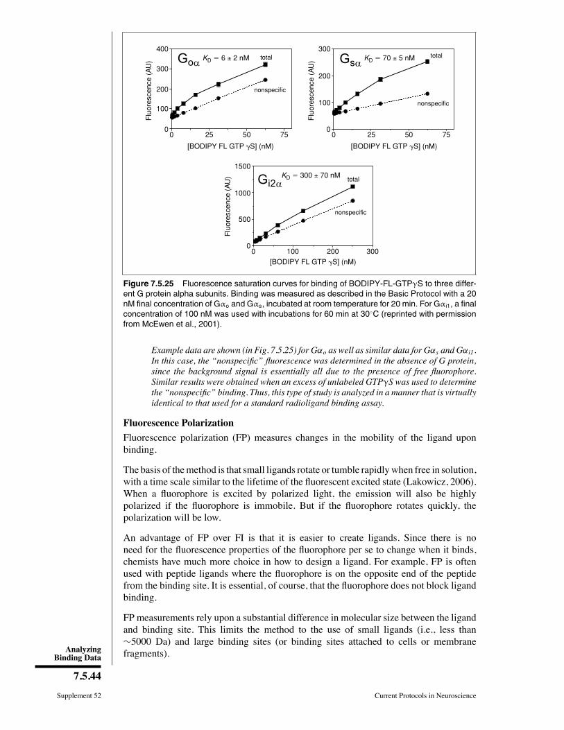
AnalyzingBinding Data
7.5.44
Supplement 52 Current Protocols in Neuroscience
[BODIPY FL GTP �S] (nM)F
luo
resc
en
ce (
AU
)
Flu
ore
sce
nce
(A
U)
Flu
ore
sce
nce
(A
U)
[BODIPY FL GTP �S] (nM)
[BODIPY FL GTP �S] (nM)
100
5000
100
200
300
0
100
200
300400
7525 500 7525
200
KD � 300 ± 70 nM
KD � 6 ± 2 nM KD � 70 ± 5 nM
300
nonspecific
nonspecific
nonspecific
total
total total
00
500
1000
1500
Figure 7.5.25 Fluorescence saturation curves for binding of BODIPY-FL-GTPγS to three differ-
ent G protein alpha subunits. Binding was measured as described in the Basic Protocol with a 20
nM final concentration of Gαo and Gαs, incubated at room temperature for 20 min. For Gαi1, a final
concentration of 100 nM was used with incubations for 60 min at 30◦C (reprinted with permission
from McEwen et al., 2001).
Example data are shown (in Fig. 7.5.25) for Gαo as well as similar data for Gαs and Gαi1.In this case, the �nonspeciÞc� ßuorescence was determined in the absence of G protein,since the background signal is essentially all due to the presence of free ßuorophore.Similar results were obtained when an excess of unlabeled GTPγS was used to determinethe �nonspeciÞc� binding. Thus, this type of study is analyzed in a manner that is virtuallyidentical to that used for a standard radioligand binding assay.
Fluorescence Polarization
Fluorescence polarization (FP) measures changes in the mobility of the ligand uponbinding.
The basis of themethod is that small ligands rotate or tumble rapidlywhen free in solution,with a time scale similar to the lifetime of the ßuorescent excited state (Lakowicz, 2006).When a ßuorophore is excited by polarized light, the emission will also be highlypolarized if the ßuorophore is immobile. But if the ßuorophore rotates quickly, thepolarization will be low.
An advantage of FP over FI is that it is easier to create ligands. Since there is noneed for the ßuorescence properties of the ßuorophore per se to change when it binds,chemists have much more choice in how to design a ligand. For example, FP is oftenused with peptide ligands where the ßuorophore is on the opposite end of the peptidefrom the binding site. It is essential, of course, that the ßuorophore does not block ligandbinding.
FP measurements rely upon a substantial difference in molecular size between the ligandand binding site. This limits the method to the use of small ligands (i.e., less than∼5000 Da) and large binding sites (or binding sites attached to cells or membranefragments).

Neurochemistry/Neuropharma-cology
7.5.45
Current Protocols in Neuroscience Supplement 52
The ßuorophore is excited with polarized light and the emission is measured with a po-larizer parallel to the excitation polarization (F‖), and also with a polarizer perpendicularto the excitation polarizer (F⊥). The difference between these twomeasurements, usuallycalculated as a polarization (P) value, is a measure of how rapidly the ßuorophore istumbling.
( ) ( )– /P F F F F⊥ ⊥= +
Equation 7.5.43
Because polarization is computed as a ratio, its value does not vary directly with the con-centration of ligand and it will not be affected by small variations in ligand concentrationor by the presence of compounds that might absorb the excitation or emission light. Thisleads to excellent reproducibility of the signal.
In theory, polarization can run from −0.33 (rapidly tumbling ligand) to 0.5 (immobileligand) (Lakowicz, 2006). In practice, measured values of polarization tend to range from0.02 to 0.30. This is usually expressed as milli-polarization units (mP = P/1000), with arange of 20 to 300 mP.
Experimentally measured ßuorescent polarization is the sum of polarization from un-bound ligand (PL) and polarization from the receptor-ligand complex (PRL). The relativeamounts of each depends on the fraction of ligand bound (F). Measured polarization (P),therefore equals:
P F P F P= − )× + ×(1 L RL
Equation 7.5.44
When the ligand concentration is low, a high fraction of ligand is bound to receptors(although a low fraction of receptors are bound to ligand). Thus F is greatest at lowligand concentrations (i.e., well below the Kd). Fluorescence polarization is greatestwhen ligands are immobile, so PRL is greater than PL. Therefore measured polarization,P, is highest at low ligand and high receptor concentrations. As shown in Fig. 7.5.26,P increases as the total receptor concentration, RT, is increased. At a Þxed receptorconcentration, as the ligand concentration (LT) increases, the free fraction of ligandincreases and P decreases (Fig. 7.5.27).
0.0 0.5 1.0 1.5
RT (nM)
Flu
ore
sce
nce
po
lari
zatio
n(m
P)
100
200
300
02.0 2.5
Kd ~ 0.16 nM
Figure 7.5.26 Fluorescence polarization measurements of αMSH binding. Fluorescent ligand
(0.5 nM BODIPY-NDP-αMSH) was incubated with increasing amounts of membrane containing
the indicated concentrations of MC5 receptor. Fluorescence polarization was measured and plotted
versus concentration of added receptor. Data from Nosjean et al. (2006).

AnalyzingBinding Data
7.5.46
Supplement 52 Current Protocols in Neuroscience
0 4
BODIPY-NDP-� MSH (nM)
Flu
ore
scence
pola
riza
tion
(mP
)
100
150
50
200
250
08 12
Kd ~ 0.43 nM
Figure 7.5.27 Fluorescence polarization measurements of αMSH binding with varying ligand.
Membranes containing 1 nM MC5 receptor were incubated with increasing amounts of fluores-
cent ligand (BODIPY-NDP-αMSH). Fluorescence polarization was measured and plotted versus
concentration of added ligand. As indicated in the text, the fraction of bound ligand (and the polar-
ization) is highest at the low ligand concentrations. These data were fitted using NLLSQ analysis
with Equation 7.5.20, with a fixed value of RT = 1.0 nM (Nosjean et al., 2006). Although the
concentration of ligand at which the polarization falls to a half-maximal value is about 2 nM, the
calculated Kd is 0.43 nM due to ligand depletion that occurs because RT>Kd.
Analysis of FP measurements: Varying receptor
Given that the binding equation L+R� LR is symmetrical for ligand and receptor, onecan determine the Kd for a binding reaction by varying the concentration of either ligandor receptor. In fact, FP binding experiments are often performed with a single low ligandconcentration (below the Kd) and various receptor concentrations (Fig 7.5.26). The halfmaximal amount of ligand bound occurs when free R is equal to the Kd. Since free ligandhas low polarization and bound ligand has high polarization, the curve (Fig 7.5.26) looksa lot like a standard saturation experiment. The added receptor binds the free ligand,leading to increased polarization. In this type of study, the fraction of bound ligand islinear with the value of P from PL (polarization of ligand alone i.e., zero ligand bound)to PRL (polarization with all ligand bound at a saturating receptor concentration). Datafrom Nosjean et al. (2006) were Þt to a standard one-site binding hyperbola to estimatea Kd value of 0.16 nM (Fig 7.5.26). One difÞculty with this approach is that one needsto know the receptor concentration from some other method (e.g., protein concentrationor radioligand binding) to get a Kd using these data alone. Also, the estimated Kd fromthis study does not take ligand depletion into account. Thus, it is surprising that half-saturation occurs at 0.16 nM, which is less than half of the concentration of the ligand(LT = 0.5 nM so half saturation should not occur at less than 0.25 nM, since you need atleast that much receptor to bind half of the ligand).
Analysis of FP measurements: Varying ligand
An alternative approach is to vary ligand concentrations. To analyze this type of data,Nosjean et al. (2006) developed an approach to Þt polarization values from the primaryexperimental parameters (LT, RT, and Kd). The following equation can be used for thispurpose (either to Þt data from single experiments or to globally Þt data from a series todetermine Kd and RT).
P P P P L L R K L R K R L= + −( )⎡⎣ ⎤⎦ × + +( )− + +( ) − × ×( )⎡⎣⎢L RL L T T T d T T d T T/
1
24
2 ⎤⎤⎦⎥
Equation 7.5.45
This equation combines the polarization equations and ligand binding functions, takinginto account the ligand depletion which is often present in ßuorescence binding methods.

Neurochemistry/Neuropharma-cology
7.5.47
Current Protocols in Neuroscience Supplement 52
With this equation, one can Þt raw polarization data obtained with variable LT withseveral different amounts of receptor to deÞne both Kd and RT.
In Figure 7.5.27, this method is applied to FP measurements of a ßuorescent ligand forthe MC5 receptor similar to those shown in Figure 7.5.26. Since the concentration ofreceptor (1 nM) is greater than the Kd, it is essential to account for depletion. So thedata were Þtted to the preceding equation using LT as the independent variable, keepingRT constant at 1 nM, and permitting all other parameters (Kd, PL, PRL) to be optimizedby the nonlinear least-squares program. The importance of including ligand depletion isclearly illustrated here. If depletion were ignored, the estimated Kd would be 1.6 nM,while the true calculated Kd based on the depletion due to the 1 nMMC5 receptor presentis only 0.43 nM.
Analysis of FP measurements: Competition
Perhaps the most useful application of FP measurements is in determining the bindingof nonßuorescent competing ligands. Since polarization provides a direct measure of thefraction of labeled ligand bound, the reduction in P by a competing ligand is directlyanalogous to a radioligand competition study. Indeed, one of the most common usesof FP is in high-throughput screening for compounds that can bind to a receptor. Theanalysis is identical to that for a radioligand competition assay, as explained earlier. Ifthe Ki value estimated using standard competition equations is less than 2 to 3 times thevalue of RT, one should include ligand depletion in the analysis.
FRET
Fluorescence resonance energy transfer (FRET) detects changes in the proximity ofthe ligand to the receptor. It is widely used in detecting protein-protein interactions,but it can also be used for measurements of ligand binding. The principle of FRETinvolves nonradiative transfer of energy from an excited donor ßuorophore (on eitherthe ligand or receptor) to an acceptor ßuorophore within about 100
◦A on the other
binding partner. Extensive information on the theory and analysis of FRET is available(Gordon et al., 1998; Lakowicz, 2006), so that will not be repeated here. Measurementstypically involve three readings, Donor, FRET, and Acceptor, where the Þrst two useexcitation at the donor wavelength and measure emission at the donor and acceptorwavelengths, respectively. The Acceptor signal is measured with both excitation andemission at the acceptor wavelength. These three measurements are combined tocalculate �corrected FRET.� This corrected FRET signal is directly proportional tothe amount of ligand bound and can be analyzed using the standard ligand bindingequations described above for FI and for radioligand binding methods. Because theinitial analysis of the raw data (as described in Gordon et al., 1998) requires appropriatecorrections for the ßuorescence from free donor and acceptor, the nonspeciÞc binding isessentially removed during that correction and Þtting can proceed as for speciÞc bindingmeasurements.
ANALYZING DATA USING NONLINEAR REGRESSION
Radioligand binding data are best analyzed using nonlinear regression to Þt curvesthrough the data.
The Problem with Using Linear Regression on Transformed Data
Before the age of microcomputers, scientists transformed their data to make a lineargraph, and then analyzed the transformed data with linear regression. Examples includeLineweaver-Burke plots of enzyme kinetic data, Scatchard plots of binding data, andlogarithmic plots of kinetic data.

AnalyzingBinding Data
7.5.48
Supplement 52 Current Protocols in Neuroscience
These methods are outdated, and should not be used to analyze data. The problem isthat the linear transformation distorts the experimental error. Linear regression assumesthat the scatter of points around the line follows a Gaussian distribution and that thestandard deviation is the same at every value of x. These assumptions are usually nottrue with transformed data. A second problem is that some transformations alter therelationship between x and y. For example, in a Scatchard plot, the value of x (bound) isused to calculate y (bound/free), and this violates the assumptions of linear regression.For an example of this, see Saturation Binding Experiments, Analysis of SaturationBinding Curves, The problem with using Scatchard plots to analyze saturation bindingexperiments).
Since the assumptions of linear regression are violated, the results of linear regression areincorrect. The values derived from the slope and intercept of the regression line are notthe most accurate determinations of the receptor number, rate constants, or dissociationconstants. Considering all the time and effort put into collecting data, the best possibleanalysis technique should be used, and nonlinear regression produces the most accurateresults.
Although linear regression is usually inappropriate for analyzing transformed data, itis often helpful for displaying transformed data because many people Þnd it easierto visually interpret linear data. This makes sense because the human eye and brainevolved to detect edges (lines), not to detect rectangular hyperbolas or exponential decaycurves.
Comparison of Linear and Nonlinear Regression
A line is described by a simple equation that calculates y from x, slope, and intercept.The purpose of linear regression is to Þnd values for the slope and intercept that deÞnethe line that best Þts the data. More precisely, it Þnds the line that minimizes the sum ofthe squares of the vertical distances of the points from the line.
The goal of minimizing the sum of squares in linear regression can be achieved quitesimply. A bit of algebra (shown in many statistics books) derives equations that deÞne thebest-Þt slope and intercept. Enter the data, perform a few calculations, and the answerscome out. There is no chance for ambiguity.
Nonlinear regression Þts data to any equation that deÞnes y as a function of x and oneor more parameters. Like linear regression, it Þnds the values of those parameters thatminimize the sum of the squares of the vertical distances of the points from the curve.With the exception of a few special cases (like linear regression), it is not possible tosolve the equations directly to Þnd the best-Þt values of the parameters. Instead, nonlinearregression requires an iterative approach that requires use of a computer.
To analyze data with nonlinear regression, the program will require an equation(model) that deÞnes y as a function of x and one or more parameters (i.e., Kd,Bmax, or rate constants). It will also require an estimate (or guess) for the best-Þtvalue for each parameter in the equation (some programs provide the initial estimatesautomatically).
Every nonlinear regression program follows these steps:
1. Using the initial values provided, the program calculates a predicted value of y foreach value of x. It then compares the actual y values with the predicted y values, andcalculates the sum of the squares of the differences between observed and predictedy values.

Neurochemistry/Neuropharma-cology
7.5.49
Current Protocols in Neuroscience Supplement 52
2. The program then adjusts the parameters to improve the Þt and reduce the sumof squares. There are several algorithms for adjusting the parameters. The mostcommonly usedmethodwas derived by Levenberg andMarquardt (often called simplythe Marquardt method), but the details of how this method works cannot be under-stood without matrix algebra. However, nonlinear regression can be used to analyzedata without knowing anything about these algorithms.
3. Step 2 is repeated. Each time the parameters are adjusted by a smaller amount. TheÞtting stops when the adjustments make virtually no difference in the sum of squares.This typically requires 5 to 20 iterations.
4. Best-Þt results are reported. The precise values obtained will depend in part on theinitial values and the stopping criteria. This means that repeat analyses of the samedata will not always give exactly the same results.
Decisions That Need to be Made When Fitting Curves with Nonlinear Regression
When using a program for nonlinear regression, the following decisions must be made.
Which equation?
An equation must be chosen that deÞnes y as a function of x and one or more parameters.This equation should represent a model, usually the law of mass action.
In many cases, the best approach is to globally Þt several data sets (to the same, ordifferent, models) sharing some parameters. Global nonlinear regression Þnds one best-Þt value for all shared parameters, and Þnds separate best-Þt values for each data set forthe other parameters.
Which units?
In pure mathematics, it does not matter whether data are entered as 1 pM or 10−12 M,as 100 fmol/mg or 60,000,000,000 receptors/mg. When computers do the calculating,however, it can matter. Calculation problems such as round off errors are far morelikely when the values are very high or very low. Scale data to avoid values <10−4or >104.
Global nonlinear regression onlymakes sense if the y values for all data sets are expressedin the same units.
Which estimated initial values?
Nonlinear regression is an iterative procedure. The program must start with estimatedvalues for each parameter that is in the right �ball park��usually within a factor of Þveof the actual value. It then adjusts these initial values to improve the Þt and repeats theadjustments until the improvement is no longer signiÞcant.
Later sections of this unit explain how to choose initial values for various kinds ofexperiments. The estimates do not need to be extremely accurate. Nonlinear regressionwill usually work Þne as long as the estimates are within 3 to 5 times their actualvalues.
Some programs (including GraphPad Prism) automatically choose initial values for you.This is a great convenience most of the time. But occasionally, the automatic initialvalues are not appropriate for the situation. The Þrst step in troubleshooting problem Þtsis to plot the curve deÞned by the initial values and make sure it goes near the data. Ifnot, you can manually adjust the initial values to make the curve better approximate thedata.
AnalyzingBinding Data
7.5.50
Supplement 52 Current Protocols in Neuroscience
Fix one or more parameters to a constant value?
In some situations it makes sense to Þx some of the parameters to constant values. Forexample, when analyzing speciÞc (rather than total) binding, the bottom plateau of adissociation experiment should be deÞned as a constant equal to zero.
Weighting
In general, the goal of nonlinear regression is to Þnd the values of the parameters in themodel that make the curve come as close as possible to the data points. Usually this isdone by minimizing the sum of the squares of the vertical distances of the data pointsfrom the curve. This is appropriate when the scatter of points around the curve is expectedto be Gaussian and unrelated to the y values of the points.
Withmany experimental protocols, the experimental scatter is not expected to be the samefor all points. Instead, the experimental scatter is expected to be a constant percentageof the y value. If this is the case, points with high y values will have more scatter thanpoints with low y values. When the program minimizes the sum of squares, points withhigh y values will have a larger inßuence while points with smaller y values will berelatively ignored. This problem may be avoided by minimizing the sum of the squareof the relative distances. This procedure is termed weighting the values by 1/y2. Becauseit prevents large points from being over-weighted, the term unweighting seems moreintuitive but weighting is the usual term used.
Data may be weighted in other ways. The goal is to obtain a measure of goodness-of-Þtthat values all the data points equal to their reliability.
With binding data, scatter is often proportional to the amount of binding, so relativeweighting may be appropriate. With good-quality data, results are usually very similarwhether or not you choose to use relative weighting.
Average replicates?
If replicate y values are collected at every value of x, there are two ways to analyze thedata: (1) treat each replicate as a separate point, or (2) average the replicate y values andtreat the mean as a single point.
With radioligand binding data, the Þrst approach is usually best, because all the dataare obtained from one tissue preparation and the sources of experimental error areindependent for each tube. If one value happens to be a bit high, there is no reasonto expect the other replicates to be high as well. Each replicate can be considered anindependent data point.
Do not treat each replicate as a separate point when the experimental error of the replicatesis related. Instead, average the replicates and analyze the averages. This situation does notcome up often with radioligand binding data, but here is one example. Assume that youperform an experiment with only a single replicate at each value of y (concentration ortime) but count each tube three times. It is not fair to enter the three counts as triplicates,and then analyze each triplicate as a separate value. As the replicates are not independent,any experimental error would appear in all the replicates.
Assumptions of Nonlinear Regression
The results of nonlinear regression are meaningful only if the following assumptions aretrue (or nearly true):
1. The model is correct. Nonlinear regression adjusts the parameters in the equation youchose to minimize the sum of squares. It does not attempt to Þnd a better equation.

Neurochemistry/Neuropharma-cology
7.5.51
Current Protocols in Neuroscience Supplement 52
2. The variability of values around the curve follows a Gaussian distribution. Eventhough no biological variable follows a Gaussian distribution exactly, it is sufÞcientthat the variation be approximately Gaussian.
3. The standard deviation (SD) of the residuals is the same everywhere, regardless ofthe value of x. In other words, the average scatter of the points around the curve is thesame at all parts of the curve. The assumption is termed homoscedasticity. If the SDis not constant but rather is proportional to the value of y, weight the data to minimizethe sum of squares of the relative distances.
4. The model assumes that x is known exactly. This is rarely the case, but it is sufÞcient toassume that any imprecision in measuring x is very small compared to the variabilityin y.
5. The errors are independent. The deviation of each value from the curve should berandom, and should not be correlated with the deviation of the previous or next point.If there is any carryover from one sample to the next, this assumption will be violated.
EVALUATING RESULTS OF NONLINEAR REGRESSION
Before accepting the results of nonlinear regression, the following questions should beasked.
Did the Program Converge on a Solution?
A nonlinear regression program will stop its iterations when it cannot improve the Þtby adjusting values of any of the parameters. At that point, the program is said to haveconverged on the best Þt. In some cases, the program gets stuck. It does not knowwhetherthe Þt would improve by increasing or decreasing the value of a parameter. When thishappens, the program stops. The exact wording of the error message is unlikely to behelpful. In this situation, some programs may still apparently show results, but these�results� do not represent a best-Þt curve.
Are the Results ScientiÞcally Plausible?
The mathematics of curve Þtting sometimes yields results that make no scientiÞc sense.For example, noisy or incomplete data can lead to negative rate constants, fractionsgreater than 1.0, and negative Kd values.
If the results make no scientiÞc sense, they are unacceptable, regardless of R2 and of howclose the curve comes to the points. Try a simpler equation, or try Þxing some parametersto constant values.
Also check that the best-Þt values of the parameters are reasonable compared to the rangeof the data. Do not trust the results if the top plateau of a sigmoid curve is far higher thanthe highest data point. Do not trust the results if an EC50 value is not within the range ofthe x values.
HowWide are the ConÞdence Intervals?
In addition to reporting the values of the parameters that make the equation Þt the databest, nonlinear regression programs also express the uncertainty as a 95% conÞdenceinterval (CI) for each parameter. If all the assumptions of nonlinear regression are true,there is a 95% chance that the interval contains the true value. More precisely, if anonlinear regression is performed many times (on different data sets), the conÞdenceintervals will include the true value 95% of the time, but exclude the true value the other5% of the time (but you will not know when that happens).

AnalyzingBinding Data
7.5.52
Supplement 52 Current Protocols in Neuroscience
Three factors can make the conÞdence interval too narrow (i.e., narrower than the truerange of parameter values):
1. The CI is based only on the scatter of data points around the curve within this oneexperiment. If the data points happen to fall right on a curve that agrees with themodel, the CI may be very small. If the experiment is repeated many times, the scatterbetween the results is likely to be greater than predicted from the CI determined inone experiment.
2. If any of the assumptions of nonlinear regression are violated, the conÞdence intervalswill probably be too narrow.
3. The conÞdence intervals from nonlinear regression are calculated using mathematicalshortcuts and so are referred to as asymptotic conÞdence intervals or approximateconÞdence intervals. In some cases, these intervals can be too narrow (too optimistic).
Because of these problems, the conÞdence intervals should not be interpreted too rig-orously. Rather than focusing on the CI reported from analysis of a single experiment,repeat the experiment several times.
If the conÞdence interval is extremely wide (e.g., > 50% of the parameter value), donot trust the results. ConÞdence intervals are wide when the data are very scattered, datahave not been collected over a wide enough range of x values, or you are Þtting too manyparameters and should constrain one or more parameters to a constant value.
The data in Figure 7.5.28 were Þt to a dose-response curve, and the 95% CI for the EC50extends over six orders of magnitude. The explanation is simple. Since the data do notdeÞne plateaus at either the top or the bottom, zero and one hundred are not deÞned. Thismakes it impossible to determine the EC50 with precision.
In this example, it might make scientiÞc sense to set the bottom plateau to 0% and thetop plateau to 100% (if the plateaus were deÞned by other controls not shown on thegraph). If this were done, the equation would Þt Þne and the conÞdence interval wouldbe narrow.
Log[dose]
Response
0
50
100
fit to sigmoidal curve
R 2 = 0.9999
Figure 7.5.28 A dose-response curve with data collected over a narrow range of concentrations.
When a nonlinear regression program tries to fit the top and bottom plateaus as well as the EC50
and slope, the resulting confidence intervals are very wide. Since there is no data to define zero
and one hundred, the program will be very uncertain about the EC50. If the nonlinear regression
program is told to set the top and bottom plateaus to constant values (from controls), then it can
determine the EC50 with precision.

Neurochemistry/Neuropharma-cology
7.5.53
Current Protocols in Neuroscience Supplement 52
100
50
0
–10 –8 –6 –4P
erc
ent re
sponse
Log[dose]
Figure 7.5.29 A dose response curve with no data in the middle of the curve. Since there are no
data points in the middle of the curve, the best-fit value of the EC50 will be uncertain with a wide
confidence interval.
Note that the problem with the Þt is not obvious by inspecting a graph, because the curvegoes very close to the points. The value of R2 (0.9999) is also not helpful. That valuealso indicates that the curve comes close to the points, but does not indicate whether theÞt is unique.
The CI is also wide when data in an important part of the curve has not been collected.The dose-response curve in Figure 7.5.29 has wide conÞdence intervals. Even whenconstraining the bottom to be zero, the top to be 100, and the slope to equal 1.0, the 95%CI for the EC50 extends over almost an order of magnitude. The problem is simple. TheEC50 is the concentration at which the response is half-maximal, and this example hasno data near that point.
Finally, the CI is wide if one tries to Þt data to a two-site model when the data reallyfollow a one-site model. In this case, the program might report very wide conÞdenceintervals, as it will report that the two sites are very similar.
Some programs report the standard error of each parameter, instead of (or in additionto) the conÞdence interval. It is not entirely straightforward to interpret the standarderror values. The best use of the standard error values is to calculate 95% conÞdenceintervals (CI), if the nonlinear regression program does not calculate one. The 95%conÞdence interval extends from approximately two standard errors below the best-Þtvalue to approximately two standard errors above the best-Þt value (the number 2.0is approximate; the exact multiplier comes from the t distribution and depends on thenumber of degrees of freedom, which equals the number of data points minus the numberof parameters Þt by the program).
Does the Curve Come Close to the Points?
In rare cases, the Þt may be far from the data points. This may happen, for example, ifthe wrong equation is chosen. Look at the graph to make sure this did not happen.
Goodness of Þt can also be evaluated by looking at the value of R2 (known by statisticiansas the coefÞcient of determination). R2 is the fraction of the total variance of y that isexplained by the model (equation). Mathematically, it is deÞned by the equation: R2 =1.0 − SS/sy
2, where sy2 is the variance (standard deviation squared) of y values. The
value of R2 is always between 0.0 and 1.0, and it has no units.

AnalyzingBinding Data
7.5.54
Supplement 52 Current Protocols in Neuroscience
When R2 equals 0.0, the best-Þt curve Þts the data no better than a horizontal line goingthrough the mean of all y values. In this case, knowing x does not help you predict y.When R2 = 1.0, all points lie exactly on the curve with no scatter; if x is known, y maybe calculated exactly.
If R2 is high, the curve comes closer to the points than would a horizontal line throughthe mean y value, but a high R2 should not be overinterpreted. It does not mean thatthe chosen equation is the best to describe the data. It also does not mean that the Þt isunique�other values of the parameters may generate a curve that Þts just as well.
When comparing one- and two-site models, it is not sufÞcient to simply compare R2
values.
It is easy to put too much importance on the value of R2. It only quantiÞes how closethe curve comes to the points. Evaluating nonlinear regression results requires lookingat more than the R2.
Do the Data Systematically Deviate from the Curve?
If the data really follow the model described by the chosen equation, the data pointsshould be randomly scattered above and below the curve. The distance of the points fromthe curve should also be random, and not be related to the value of x.
The best way to look for systematic deviations of the points from the curve is to inspecta graph of the residuals and to look at the runs test.
Residuals
A residual is the distance of a point from the curve. A residual is positive when the pointis above the curve, and is negative when the point is below the curve. The residual tablehas the same x values as the original data, but each y value is replaced by the verticaldistance of the point from the curve. An example is shown in Figure 7.5.30. As shown inpanel A, the data points are not randomly distributed above and below the curve. Thereare clusters of points all above or all below. This is much easier to see on the graph inpanel B. The points are not randomly scattered above and below the x axis.
The runs test
The runs test determines whether the data deviate systematically from the equation youselected. A run is a series of consecutive points that are either all above or all below theregression curve. Another way of saying this is that a run is a series of points whoseresiduals are either all positive or all negative.
If the data points are randomly distributed above and below the regression curve, it ispossible to calculate the expected number of runs. If there are fewer runs than expected,it may mean that the regression model is wrong. If the data really follow the equationused to create the curve, the P value from the runs test may be used to determine thechance of obtaining as few (or fewer) runs as observed in the experiment. If the P valueis small, it indicates that the data really do not follow the model.
In the example in Figure 7.5.30, the equation does not adequately match the data. Thereare only six runs, and the P value for the runs test is very small. This means that the datasystematically deviate from the curve, and the data were Þt to the wrong equation.
The replicates (or lack of Þt) test
When evaluating a nonlinear Þt, one question you might ask is whether the curve is �toofar� from the points. The answer, of course, is another question: too far compared to

Neurochemistry/Neuropharma-cology
7.5.55
Current Protocols in Neuroscience Supplement 52
50
100
150
Sig
na
l
R 2 = 0.97Number of runs = 6P value = 0.0025
0
�10
�20
Time
Re
sid
ua
ls
20
10
0
2.5 5.0 7.5 10.0 12.5 15.0 17.5 20.00.0
A
B
Figure 7.5.30 Residuals. The top panel (A) graphs dissociation kinetic data. The bottom panel
(B) shows the residuals (i.e., the y axis plots the distance between the point and the curve from
the top panel).
what? If you have collected one y value at each x value, you can�t really answer thatquestion (except by referring to other similar experiments). But if you have collectedreplicate y values at each x, then you can ask whether the average distance of the pointsfrom the curve is �too far� compared to the scatter among replicates.
If the P value is low, it means that the scatter of the points around the best-Þt curve ismuch greater than predicted by the scatter among the replicates. This is evidence that thedata may actually follow a model that is different than the model that you chose (or thatthe replicates are not fully independent from one another).
If the P value is high, it means the scatter of points from the curve is entirely consistentwith the scatter among the replicates. There is no reason (based on this test) to questionthe validity of the model. You should not conclude that you have chosen the best pos-sible model. But you can conclude that the Þt of the model is entirely consistent withexpectations from the scatter among replicates within the range of x values you chose touse.
Is the Fit a Local Minimum?
The nonlinear regression procedure adjusts the parameters in small steps in order toimprove the goodness of Þt. If GraphPad Prism converges on an answer, altering any ofthe parameters a little bit will make the Þt worse. But it is theoretically possible that largechanges in the parameters might lead to much better goodness of Þt. Thus, the curve thatPrism decides is the �best� may really not be the best.

AnalyzingBinding Data
7.5.56
Supplement 52 Current Protocols in Neuroscience
Su
m o
f sq
ua
res
Value of variable
starting here, result
will be best-fit
starting here, result
will be false minimum
best fitfalse minimum
Figure 7.5.31 What is a false minimum? A nonlinear regression program stops when making
any small change to a parameter will worsen the fit and thus raise the sum of squares. In rare
cases, this may happen at a false minimum rather than the true best fit value.
Think of latitude and longitude as representing two parameters Prism is trying to Þt.Now think of altitude as the sum of squares. Nonlinear regression works iteratively toreduce the sum of squares. This is like walking downhill to Þnd the bottom of the valley.When nonlinear regression has converged, changing any parameter increases the sum ofsquares. When at the bottom of the valley, every direction leads uphill. But there maybe a much deeper valley over the ridge that is unknown (see Fig. 7.5.31). In nonlinearregression, large changes in parameters might decrease the sum of squares.
This problem (called Þnding a local minimum) is intrinsic to nonlinear regression, nomatter what program is used. A local minimum will rarely be encountered if the datahave little scatter, the data are collected over an appropriate range of x values, and anappropriate equation is chosen.
To continue the analogy, the conÞdence intervals for the parameters are very wide whenthe bottom of the valley is very ßat. A great distance can be traveled without changingelevation. The values of the parameters can be changed a great deal without changingthe goodness of Þt.
To test for the presence of a false minimum:
1. Look at the Þtted curve and see if it comes close to the data or if it deviates system-atically (also check runs and replicates tests). Such systematic deviations may resulteither from an incorrect model or from convergence to a local minimum.
2. Note the values of the parameters and the sum of squares from the Þrst Þt.
3. Make a large change to the initial values of one or more parameters and run the Þtagain. Repeat several times.
4. Ideally, nonlinear regression will report nearly the same sum of squares and sameparameters regardless of the initial values. If the values are different, accept the oneswith the lowest sum of squares.
What to Do When the Fit Is No Good?
The previous sections explained how to identify a bad Þt. If any of these situations areencountered, Table 7.5.11 describes some things to try.

Neurochemistry/Neuropharma-cology
7.5.57
Current Protocols in Neuroscience Supplement 52
Table 7.5.11 Troubleshooting Guide to Evaluating Results of Nonlinear Regression
Potential problem Solution
The equation simply does not describe thedata.
Try a different equation.
The initial values are too far from their correctvalues.
Enter different initial values. If using auser-deÞned equation, check the rules for initialvalues.
The range of x values is too narrow to deÞnethe curve completely.
If possible, collect more data. Otherwise, holdone of the variables to a constant value.
There is not enough data collected in a criticalrange of x values.
Collect more data in the important regions.
The data are very scattered and don�t reallydeÞne a curve.
Try to collect less scattered data. If combiningseveral experiments, normalize the data for eachexperiment to an internal control.
The equation includes more than onecomponent, but the data don�t follow amulticomponent model.
Use a simpler equation.
The numbers are too large. If the y values are very large, change the units.Do not use values greater than ∼104.
The numbers are too small. If your y values are very small, change theunits. Do not use values less than ∼10−4.
Table 7.5.12 Log(Ki) Values for a Sample
Competitive Binding Experiment
Experiment Control Treated
1 −6.13 −6.532 −6.39 −6.863 −5.92 −6.31
COMPARING TREATMENT GROUPS
The results of radioligand binding experiments will often be compared between treatmentgroups. There are three ways to do this.
Compare the Results of Repeated Experiments
After repeating the experiment several times, compare the best-Þt value of a parameterfor each Þt of control and treated preparations using a paired t test (or the analogousWilcoxon nonparametric test).
For example, in Table 7.5.12, the log(Ki) values of results from a competitive bindingcurve performed with two groups of cells are shown. Compare the results using a pairedt test. The t ratio is 16.7, and the P value is 0.0036 (two-tail). If the treatment did notalter the log(Ki), there is only a 0.36% chance that such a large difference (or larger)between log(Ki) is by chance. Since the P value is so low, conclude that the change in Kiwas statistically signiÞcant.
Note that we compare log(Ki) values rather than Ki values. When doing a paired ttest, a key assumption is that the distribution of differences (treated versus control)follow a Gaussian distribution. Since a competitive binding curve (similar to a dose

AnalyzingBinding Data
7.5.58
Supplement 52 Current Protocols in Neuroscience
response curve) is conducted with x values (concentration) equally spaced on a log scale,the uncertainty of the EC50 is reasonably symmetrical (and perhaps Gaussian) whenexpressed on a log scale. It is equally likely that the best-Þt value of the log (Ki) is0.1 log units too high or 0.1 log units too low. In contrast, the uncertainty in Ki is notsymmetrical.
Compare the Results Within One Experiment: Extra Sum-of-Squares Approach
To compare two curves, Þrst Þt the two curves separately, and then Þt all the dataglobally to Þt one curve to all the data. Comparing the sum of the sum of squares withthe independent Þt to the sum of squares for the global Þt can result in a P value thatcompares the Þts (Munson and Robard, 1980).
For example, competitive binding curves of control and treated cells were compared inan experiment performed once. Nonlinear regression Þt three parameters, Top, Bottom,and log(EC50). Only the log(EC50) values are of interest. In this example, the controllog(EC50) was −6.08 with a standard error of 0.3667. The treated log(EC50) was −6.20with a standard error of 0.0617.
GraphPad Prism can compare two Þts with the extra sum-of-squares F test by checkingan option. The instructions below assume that you are using a program that cannot dothe comparison automatically. It is also useful to follow these steps to understand howthe approach works.
1. Fit the two data sets separately as in the previous section.
2. Total the sum of squares and DF from the two Þts. For this example the total sumof squares equals 19,560 + 29,320 = 48,880, and the total DF equals 12 + 12 = 24.Since these are the results of Þtting the two data sets separately, label these valuesSSseparate and DFseparate.
3. Combine the two data sets into one. For this example, the combined data set has 30xy pairs, with each x value appearing twice.
4. Fit the combined data set to the same equation. Note the SS and DF. For this example,SS= 165,200, and DF= 27 (30 data points minus three parameters). Call these valuesSScombined and DFcombined.
5. SSseparate is expected to be smaller than SScombined even if the curves are really identical,simply because the separate Þts have more degrees of freedom. Two separate curveswill always come closer to the points than one combined curve. The question iswhetherthe SS values are more different than expected by chance. To Þnd out, calculate the Fratio using the equation:
F =−⎛
⎝⎜⎞⎠⎟
−SS SS
SS
DF DFcombined separate
combined
combined separatte
separateDF
⎛
⎝⎜⎞
⎠⎟
Equation 7.5.46
For this example, F = 19.03.
6. Determine theP value fromF. There are 3 degrees of freedom (DFcombined−DFseparate)in the numerator, and 24 degrees of freedom (DFseparate) in the denominator. Use thefree QuickCalc Web calculator at http://www.graphpad.com, or this Excel formula:
= FDIST(19.03, 3, 24)

Neurochemistry/Neuropharma-cology
7.5.59
Current Protocols in Neuroscience Supplement 52
7. For this example, the P value is <0.0001. If the treatment is really ineffective, thereis less than 0.01% chance that the two curves would differ as much (or more) as theydiffered in this experiment. Since the P value is low, you�ll conclude that the curvesare really different.
This method only uses data from one experiment. Despite the impressively low P value,these results should not be trusted until the experiment is repeated. This method comparesthe curves overall. It does not determine which parameter(s) are different. Differencesmight be due to something trivial such as a different baseline, rather than somethingimportant such as a different EC50.
Compare the Results Within One Experiment: t Test Approach
Since each best-Þt value of a parameter is reported with a conÞdence interval (CI) anda standard error, a t test can determine whether the difference between best-Þt values isgreater than what would be expected by chance.
Compare the two groups with an unpaired t test.
1. Calculate the t ratio as the difference between log(EC50) values divided by the standarderror of that difference (calculated from the two standard errors). Since the samplesize is the same in the two groups, use the equation:
t =− ( )( )
+=
log log.
EC EC
SEM SEM
A B
A B
50 50
2 22 292
Equation 7.5.47
2. Calculate the number of degrees of freedom (DF), which equals the sum of the numberof degrees of freedom in each group. This equals the number of data points minusthe number of parameters Þt by the nonlinear regression procedure. In this example,there were 15 data points, and three parameters were Þt. So there are 12 DF in eachgroup, and 24 DF altogether.
3. To determine the P value that corresponds to the values of t and DF, use the freeQuickCalc Web calculator at http://www.graphpad.com or this Excel formula (theÞrst parameter is t, the second is DF, and the third is always 2, since you want atwo-tail P value):
=TDIST(2.292,24,2)
For this example, the P value is 0.0309. If the treatment really didn�t alter the EC50, thereis only a 3.09% chance that this large of a difference (or more) is by coincidence. Sincethe P value is so low, it is concluded that the two EC50 values are statistically signiÞcantlydifferent.
You don�t need to do the calculations manually. GraphPad Prism, GraphPad InStat, andmany other programs can compute t and the P value from data entered as mean, standarderror of the mean (SEM), and N. Enter the best-Þt value of the log(EC50) (or any other Þtparameter) instead of the mean, and the standard error (SE) of that parameter instead ofthe SEM. The trick is Þguring out what value to enter as �N� (sample size). Rememberthat:
1. For nonlinear regression, the number of degrees of freedom equals the number of datapoints minus the number of parameters Þt.

AnalyzingBinding Data
7.5.60
Supplement 52 Current Protocols in Neuroscience
2. For an ordinary t test, the number of degrees of freedom for each sample equals oneless than the number of data points.
3. The t test calculations are based on the numbers of degrees of freedom. However,most programs ask for N instead, and then compute DF as N − 1. When comparingthe results of nonlinear regression, enter N as the number of degrees of freedom plus1. The program will subtract 1 to determine the DF. All the other calculations arebased on the value of DF, and N is ignored. In this example, enter N = 12 + 1 = 13for each group.
This method only uses data from one experiment. The SE value is a measure of howprecisely the log(EC50) has been determined in this one experiment. It is not a measure ofhow reproducible the experiment is. Despite the impressive P value, these results shouldnot be trusted until the experiment is repeated.
The t test assumes that the uncertainty in the values of the parameters follows a Gaussiandistribution. This assumption is not necessarily true with the SE values that emerge fromnonlinear regression. The only way to assess the validity of this assumption is to simulatemany sets of data, Þt each with nonlinear regression, and examine the distribution ofbest-Þt values. This has been done with many commonly used equations, and it seemsthat the assumption is reasonable in many cases.
To avoid this problem when Þtting binding data, compare log(EC50), not EC50. Youwant to express the parameters in a form that makes the uncertainty as symmetrical andGaussian as possible. In general, the uncertainty of log(EC50), but not of EC50 itself, isreasonably symmetrical (and perhaps Gaussian). It is equally likely that the observedlog(Ki) is 0.1 log units too high or 0.1 log units too low. In contrast, the uncertainty in Kiis not symmetrical.
Advantages and Disadvantages of the Three Approaches
If the experiment has been repeated several times, use the Þrst method (Comparing theResults of Repeated Experiments). There are two advantages. The Þrst is that comparedto the other methods discussed, this method is far easier to understand and communicateto others. Second, the entire test is based on the consistency of the results between repeatexperiments. Since there are usually more causes for variability between experimentsthan within experiments, it makes sense to base the comparison on differences betweenexperiments.
The disadvantage of the Þrst method is that information is being discarded. The calcula-tions are based only on the best-Þt value from each experiment, and they ignore the SEof those values presented by the curve Þtting program.
If the experiment has been performed only once, the experiment should be repeated.Regardless of what statistical results are obtained, results from a single experiment shouldnot be trusted. To compare results in a single experiment, the extra sum-of-squares F testis a better test (but a bit more work) than the t test.
Generally, only one parameter is of interest (i.e., a rate constant or EC50); the othersare less important. The t test compares only the parameter you care about. The extrasum-of-squares F test is more general. Since that method compares the entire curve,it does not force a decision regarding which parameter(s) to compare. This is both itsadvantage and disadvantage.

Neurochemistry/Neuropharma-cology
7.5.61
Current Protocols in Neuroscience Supplement 52
CALCULATIONS WITH RADIOACTIVITY
EfÞciency of Detecting Radioactivity
EfÞciency is the fraction of radioactive disintegration that is detected by the counter.EfÞciency is determined by counting a standard sample under conditions identical tothose used in the experiment.
With 125I, the efÞciency is usually>90%, depending on the geometry of the counter. TheefÞciency is not 100% because the detector does not entirely surround the tube, whichallows a few gamma rays (photons) to miss the detector.
With tritium (3H), the efÞciency of counting is much lower, and usually varies between30% and 50%. The low efÞciency is mostly a consequence of the physics of decayand cannot be improved by better instrumentation or better scintillation ßuid. When atritium atom decays, a neutron converts to a proton and the reaction emits an electronand neutrino. The energy released is always the same, but it is randomly partitionedbetween the neutrino (not detected) and an electron (detection attempted). When theelectron has sufÞcient energy, it will travel far enough to encounter a ßuor molecule inthe scintillation ßuid. This ßuid ampliÞes the signal and gives off a ßash of light detectedby the scintillation counter. The intensity of the ßash (number of photons) is proportionalto the energy of the electron. If the electron has insufÞcient energy, it is not captured bythe ßuor and is not detected. If it has low energy, it is captured but the light ßash has fewphotons and is not detected by the instrument. Since the decay of many tritium atomsdoes not lead to a detectable number of photons, the efÞciency of counting is much lessthan 100%.
The efÞciency of counting 3H is reduced by the presence of any color in the counting tubes,if the mixture of water and scintillation ßuid is not homogeneous, or if the radioactivityis trapped in the tissue (thus emitted electrons do not travel into the scintillation ßuid).
SpeciÞc Radioactivity
Radioligand packaging usually states the speciÞc radioactivity as Curies per millimole(Ci/mmol). Because measurements are expressed in counts per minute (cpm), the speciÞcradioactivity is more useful when stated in cpm. Often, for radioligand binding exper-iments, it is useful to express the speciÞc radioactivity as cpm/fmol (1 fmol = 10−15mol).
To convert from Ci/mmol to cpm/fmol, know that 1 Ci equals 2.22× 10¹² disintegrationsperminute (dpm).Use this equation to convertZCi/mmol toY cpm/fmolwhen the counterhas an efÞciency (expressed as a fraction) equal to E.
Y Z Ecpm
fmol mmol
dpm
Ci
mmol
fmol
cpm
dpm= × × × ×−Ci
.2 22 10 1012 12
Equation 7.5.48
Y Z E= × × ( )2 22. in cpm fmol
Equation 7.5.49
For example, the speciÞc activity will be 2190 Ci/mmol if every molecule incorporatesexactly one 125I atom. If the counting efÞciency is 85%, then the speciÞc activity is 2190× 2.22 × 0.85 = 4133 cpm/fmol.

AnalyzingBinding Data
7.5.62
Supplement 52 Current Protocols in Neuroscience
In many countries, radioligand packaging states the speciÞc radioactivity in GBq/mmol,rather than Ci/mmol. To convert to cpm/fmol, you need to know that 1 Bq (Becquerel) isone radioactive disintegration per second (1 GBq= 109 dps). To convert fromGBq/mmolto cpm/fmol, use this equation:
Y Z Ecpm
fmol
GBq
mmol
dps
GBq
mmol
fmol
counts= × × × ×10 60 109 2sec
min ddisintegrations= × ×Z E0 06.
1
Equation 7.5.50
If every molecule is labeled with 125I, the speciÞc activity is 81,030 GBq/mmol. If thecounting efÞciency is 85%, then the speciÞc activity can also be expressed as 81,030 ×0.06 × 0.85 = 4133 cpm/fmol.
Calculating the Concentration of the Radioligand
Rather than trust dilutions, the concentration of radioligand in a stock solution canbe accurately calculated. Measure the cpm in a small volume of solution and use thefollowing equation, in which C is cpm counted, V is volume of the solution in ml, and Yis the speciÞc activity of the radioligand in cpm/fmol (calculated in the previous section).
concentration in pMcpm
cpm fmol
ml
pmol fmol
lite
=×C
Y
V
0 001
0 001
.
. rr ml
= C Y
V
Equation 7.5.51
Radioactive Decay
Radioactive decay is entirely random. The probability of decay at any particular interval isthe same as the probability of decay during any other interval. StartingwithN0 radioactiveatoms, the number remaining at time t is:
N N et
k t= × −0
decay
Equation 7.5.52
The rate constant of decay (kdecay) is expressed in units of inverse time. Each radioactiveisotope has a different value of kdecay. The value e refers to the base of natural logarithms(2.71828).
The half-life (t1 / 2) is the time it takes for half the isotope to decay. Half-life and thedecay rate constant are related by this equation:
tk k1 2
2 0 693= =ln( ) .
decay decay
Equation 7.5.53
Table 7.5.13 shows the half-lives and rate constants for commonly used radioisotopes.The table also shows the speciÞc activity assuming that each molecule is labeled withone radioactive atom. This is often the case with 125I and 32P. Tritiated molecules oftenincorporate two or three tritium atoms, which increases the speciÞc radioactivity.

Neurochemistry/Neuropharma-cology
7.5.63
Current Protocols in Neuroscience Supplement 52
Table 7.5.13 Half-Lives and Rate Constants for Commonly Used Isotopes
Isotope Half-life kdecay SpeciÞc radioactivity
3H 12.43 years 0.056 year−1 28.7 Ci/mmol125I 59.6 days 0.0116 day−1 2190 Ci/mmol32P 14.3 days 0.0485 day−1 9128 Ci/mmol35S 87.4 days 0.0079 day−1 1493 Ci/mmol
Radioactive decay can be calculated from a date where you knew the concentration andspeciÞc radioactivity using the equation:
fraction remaining decay= −e
k t
Equation 7.5.54
For example, after 125I decays for 20 days, the fraction remaining equals 79.5%.Althoughdata appear to be scanty, most scientists assume that the energy released during decaydestroys the ligand so it no longer binds to receptors. Therefore, the speciÞc radioactivitydoes not change over time.What changes is the concentration of ligand. After 20 days, theconcentration of the iodinated ligand is 79.5% of what it was originally, but the speciÞcradioactivity remains 2190 Ci/mmol. This approach assumes that the unlabeled decayproduct is not able to bind to receptors and has no effect on the binding. Rather than trustthis assumption, use newly synthesized or repuriÞed radioligand for key experiments.
Calculations of radioactive decay are straightforward only when each molecule is labeledwith a single radioactive isotope, as is usually the case. If a molecule is labeled withseveral radioactive isotopes, the effective half-life is shorter. If only a fraction of themolecules are labeled with a radioactive isotope, then the decay formula only applies tothe labeled portion of the mixture, as the concentration of the unlabeled compound neverchanges.
Counting Error and the Poisson Distribution
The decay of a population of radioactive atoms is random, and therefore subject to asampling error. For example, the radioactive atoms in a tube containing 1000 cpm ofradioactivity will not give off exactly 1000 counts in every minute. There will be morecounts in some minutes and fewer in others, with the distribution of counts following aPoisson distribution. This variability is intrinsic to radioactive decay (or any stochasticprocess) and cannot be reduced bymore careful experimental controls (but can be reducedby counting for a longer time to accumulate more events). There is no way to know the�real� number of counts, but a range of counts can be calculated that is 95% certain tocontain the true average value. As long as the number of counts (C) is greater than∼100,the conÞdence interval can be calculated using this approximation:
95 1 96 1 96% : . .CI toC C C C−( ) +( )
Equation 7.5.55
Computer programs can calculate amore exact conÞdence interval, as becomes necessarywhenC is less than∼100. For example, ifC= 100, the simple equation above calculates a95% conÞdence interval from approximately 80 to 120. Amore exact equation calculatesan interval from 81.37 to 121.61.

AnalyzingBinding Data
7.5.64
Supplement 52 Current Protocols in Neuroscience
Table 7.5.14 Determination of Confidence Values
1 min 10 min 100 min
Counts per min (cpm) 100 100 100
Total counts 100 1000 10000
95% CI of counts 81.4 to 121.6 938 to 1062 9804 to 10196
95% CI of cpm 81.4 to 121.6 93.8 to 106.2 98.0 to 102.0
1.96 √C
CPercent error = 100 x
102 103 104 105 106
Counts
0.1
1.0
10.0
100.0
Perc
ent err
or
Figure 7.5.32 Counting error. With more counts, the fractional counting error decreases. The xaxis shows the number of radioactive decays actually counted (counts per minute times number
of minutes).
When calculating the conÞdence interval, set C equal to the total number of counts youmeasured experimentally, not the number of counts per minute.
For example, if a radioactive sample is placed into a scintillation counter for 10 min, thecounter detects 225 counts per minute. What is the 95% conÞdence interval? Since thetotal timewas 10min, the instrumentmust have detected 2250 radioactive disintegrations.The 95% conÞdence interval of this number extends from 2157 to 2343. This is theconÞdence interval for the number of counts in 10 min, so the 95% conÞdence intervalfor the average number of counts per minute extends from 216 to 234. That is, there is a95% certainty that the average cpm value lies within this range.
The Poisson distribution explains why it is helpful to count samples longer when thenumber of counts is small. For example, Table 7.5.14 shows the conÞdence interval for100 cpm counted for various times. When longer times are used, the conÞdence intervalis narrower.
Figure 7.5.32 shows percent error as a function of C. Percent error is deÞned from thewidth of the conÞdence interval divided by the number of counts. Of course this graphonly shows error due to the randomness of radioactive decay. This is only one source oferror in most experiments.

Neurochemistry/Neuropharma-cology
7.5.65
Current Protocols in Neuroscience Supplement 52
ANALYZING DATAWITH GraphPad PRISM
GraphPad Prism is a general-purpose program for scientiÞc graphics, statistics andnonlinear regression, available for both Windows and Macintosh computers.
While Prism is not designed especially for analyses of binding data, it is very wellsuited for such analyses. It provides a menu of commonly used equations, including allequations listed in this unit, and can automatically compare one- and two-site modelswith an F test. When analyzing competitive binding curves, Prism calculates the Ki fromthe IC50. It can globally Þt a family of curves at once, sharing speciÞed parametersamong the curves. The program can automatically create a residual plot and calculate theruns test and replicates test. In addition, Prism�s manual and help screens, like this unit,explain the principles of curve Þtting.
A trial version of the Windows or Mac versions of Prism can be obtained from theGraphPad Web site at http://www.graphpad.com. The trial version is fully functional for30 days.
LITERATURE CITED
Cheng, Y. and Prusoff, W.H. 1973. Relationship between the inhibition constant (Ki) and the concentrationof an inhibitor that causes a 50% inhibition (I50) of an enzymatic reaction.Biochem. Pharmacol. 22:3099-3108.
Gordon, G.W., Berry, G., Liang, X.H., Levine, B., andHerman, B. 1998. Quantitative ßuorescence resonanceenergy transfer measurements using ßuorescence microscopy. Biophys. J. 74:2702-2713.
Kenakin, T. 2006. A Pharmacology Primer, Second Edition: Theory, Applications, and Methods. AcademicPress, San Diego.
Lakowicz, J.R. 2006. Principles of Fluorescence Spectroscopy, 3rd ed., Springer, New York.
Limbird, L.E. 2004. Cell Surface Receptors: A Short Course in Theory and Methods, 3rd ed. Springer, NewYork.
McEwen, D.P., Gee, K.R., Kang, H.C., and Neubig, R.R. 2001. Fluorescent BODIPY-GTP analogs: Real-time measurement of nucleotide binding to G proteins. Anal. Biochem. 291:109-117.
Motulsky, H.J. and Mahan, L.C. 1984. The kinetics of competitive radioligand binding predicted by the lawof mass action. Mol. Pharmacol. 25:1-9.
Munson, P.J. and Rodbard, D. 1980. Ligand: A versatile computerized approach to characterization of ligandbinding systems. Anal. Biochem. 107:220-239.
Neubig, R.R. and Cohen, J.B. 1979. Equilibrium binding of [3H]tubocurarine and [3H]acetylcholine byTorpedo postsynaptic membranes: Stoichiometry and ligand interactions. Biochemistry 18:5464-5475.
Nosjean, O., Souchaud, S., Deniau, C., Geneste, O., Cauquil, N., and Boutin, J.A. 2006. A simple theoreticalmodel for ßuorescence polarization binding assay development. J. Biomol. Screen. 11:949-958.
Roman, D.L., Talbot, J.N., Roof, R.A., Sunahara, R.K., Traynor, J.R., and Neubig, R.R. 2007. IdentiÞcationof small-molecule inhibitors of RGS4 using a high-throughput ßow cytometry protein interaction assay.Mol Pharmacol. 71:169-175.
Rosenthal, H.E. 1967. A graphic method for the determination and presentation of binding parameters incomplex systems. Anal. Biochem. 20:525-532.
Swillens, S. 1995. Interpretation of binding curves obtained with high receptor concentrations: Practical aidfor computer analysis.Mol. Pharmacol. 47:1197-1203.