The Royal Veterinary and Agricultural University Food and Resource Economic Institute

Optimizing Production under Uncertainty: Generalisation of the State-Contingent Approach and Comparison of Methods for Empirical Application. September 2004 Svend Rasmussen U

nit o

f Eco

nom

ics W

orki

ng P

aper

s 200

4/2

2

Optimizing Production under Uncertainty: Gener‐alisation of the State‐Contingent Approach and Comparison of Methods for Empirical Application. Svend Rasmussen Food and Resource Economic Institute The Royal Veterinary and Agricultural University (KVL) Copenhagen, Denmark Abstract In a recent paper Rasmussen (Rasmussen 2003) derived criteria for optimal production under uncertainty based on the state‐contingent approach developed by Chambers and Quiggin (2000). While the criteria in the 2003‐paper were derived for the one variable input case, and for different types of input, the present paper generalises the results to the multi‐variable input case. It is further shown that with the output‐cubical technology as the basic model, any type of input may be analysed as a special case within the gen‐eral model framework developed. The main part of the paper is devoted to the problems of empirical application of the state‐contingent approach. To empirically apply the optimization criteria derived, one needs specific functional forms of both the state‐contingent production functions and the utility function based on state‐contingent income measures. The paper shortly re‐views the empirical approach normally taken when using the well‐known Expected Utility (EU) model and this approach is in turn compared to the more general approach potentially available in the state‐contingent model. Comparisons show that the potential benefit of the state‐contingent approach compared to the expected utility model is limited by the empirical opportunities. Thus, it is unreal‐istic to expect production functions to be estimated for all possible states of nature. State‐contingent production functions therefore, have to be considered as stochastic production functions. In this case, it is not obvious whether the state‐contingent ap‐proach is better than the expected utility model, and it is proposed that this is further investigated using Monte‐Carlo simulation.

3

1. Introduction The classical approach to the problem of optimising production under risk/uncertainty is the expected utility model (EU model). The EU‐model is, in its basic form, a relatively general model. But as regards empirical application, the tradition has developed over time to the EU‐model being the equivalent of a model, where utility is maximized as a function of the expected value and variance of profit (Robison and Barry 1987; Dillon and Anderson 1990; Hardaker et al. 1997). This approach to decision making under uncertainty, has been severely criticized by Chambers and Quiggin in their book on state‐contingent production from 2000, as well as in subsequent papers. The main problem being that the traditional approach typically does not consider the interaction between the uncontrolled (uncertain) variables and the decision variables controlled by the decision maker. Furthermore, although Dillon and Anderson (1990) realised the basic need for modelling this kind of interaction, they did not derive criteria for optimal production that went beyond maximizing utility, defined as a function of expected value and variance of profit. With the state‐contingent approach developed by Chambers and Quiggin (2000), the foundation for alternative ways of describing and analysing production under uncer‐tainty, were made available. The state‐contingent approach has the advantage that it ex‐plicitly considers the interaction between controllable inputs and uncontrolled inputs (the uncertain states of nature). In a recent article, Rasmussen (2003) used the state‐contingent approach to derive criteria for optimal production (input use) under uncer‐tainty. Criteria were derived for the one variable input case, as well as for different types of input, including state‐specific and state‐allocable input. While the article illustrates that the state‐contingent approach has the merit of being based on well‐known marginal principles and optimisation tools, it also indicates that the state‐contingent approach has its own weaknesses when it comes to empirical application. Thus, the basic problem of not knowing the decision makers’ utility function still exists, and the problem of how to estimate state‐contingent production functions, has not been solved. Thus, the question of how to apply the theory of state‐contingent production to the real problems of actual decision making still has no clear answer. The objectives of this paper are to further develop and generalise the criteria for optimal production under uncertainty derived in Rasmussen (2003), and to discuss alternative procedures for empirical application. In the first part of the paper (Section 2), the criteria derived by Rasmussen (2003) are generalised to the multi‐variable input case. Further, it is shown that the output‐cubical

4

technology approach criticized by Chambers and Quiggin for not being able to model substitution between state‐contingent outputs, is in fact an appropriate vehicle to use, even in the case of state‐allocable inputs. It is shown that state‐specific and state‐allocable inputs are just special cases of state‐general inputs, and specific criteria for these two types of input are in fact superfluous; the general criteria derived will cover any type of input. The second part of the paper (Section 3) focuses on the problems related to empirical application of the state‐contingent theory. The state‐contingent approach is compared to the Expected Utility (EU) model, both with respect to choice of utility function and de‐scription of production technology (production function). In this context, the differences between state‐contingent and stochastic production functions are discussed, and it is pro‐posed that in empirical contexts, it is appropriate to consider state‐contingent production functions as being themselves stochastic production functions. The paper concludes in Section 4 with a case illustrating the application of the state‐contingent approach, in which the results demonstrate the possible consequences of the interaction between application of input and state of nature.

2. General criteria for optimal production Consider a producer who wants to optimize the production of one or more outputs. Both the production and the output prices are uncertain in the sense that yields and prices depend on uncertain future conditions called states of nature. The state of nature that determines yields and prices reveals itself only after application/allocation of input. Therefore, production decisions have to be taken without knowing the future state of nature. The only thing known about the future state is that nature will pick one of S pos‐sible states of nature. Probabilities of each state of nature may or may not be available, but the decision maker holds ‐ at least implicitly ‐ expectations concerning the frequency with which each possible state of nature will prevail. The decision‐maker wants to maximize the utility function: W = W(q) = W(q1, …, qS) (1) where W is a continuously differentiable non‐decreasing, quasi‐concave function, and q=(q1, …, qS) is a vector of net‐incomes in the S possible states of nature, determined as:

5

1 1

M nF

s ms ms i i sm i

q z p w x c k= =

= − − +∑ ∑ (s=1,…, S) (2)

where zms is production of output m in state s, pms is the price of output m in state s, xi is

the amount of variable input i (i=1,…, n) used in the pro‐duction of the M outputs, wi is the price of input i (i=1,…, n), cF is fixed costs, and ks is a state‐contingent income from other sources. First consider the case in which no production takes place. In this case, the wealth is determined by the net‐income vector: F

s sq k c= − (s=1,…, S) which is illustrated for S=2 in Figure 1. The curve aa is the income possibility curve without production. Thus,

the choice (k1‐cF, k2‐cF) in Figure 1 provides the highest utility possible without produc‐tion1). To supplement the income ks‐cF (s=1,…, S) the decision‐maker may carry out production. The production technology is, as a starting point, given in implicit form as a convex function H: M S N× +

+ℜ →ℜ : H(z, x) = H(z11, …, zms, …, zMS, x1, …, xN) ≤ 0 (3) where z is a M×S matrix of state‐contingent output of M products (z11,…, zMS) and x is a vector of input (x1, …, xN), of which the first n elements are variable inputs, and the last N – n elements are fixed inputs. The amount of fixed inputs is restricted by:

1 ) For convenience, it is assumed that aa is a quasi-convex function as indicated

q1 a k1‐cF

q2

a

k2‐cF

Figure 1. Wealth without production

W(q)=w

Indifference curve

6

1

0M

Fjm j

mx x

=

− ≤∑ (j = n+1,…, N) (4)

where xjm is the amount of fixed input j allocated to production of output m and F

jx is the amount of fixed input j. If a budget restriction applies, then:

0

10

n

i ii

w x C=

− ≤∑ (5)

where C0 is the given budget. The production plan which maximizes utility in (1) is determined by the amount of vari‐able inputs (x1, …, xn), the amount of outputs (z11, …, zms, …, zMS) and the allocation of the fixed inputs (xn+1, …, xN) which maximizes the Lagrangian:

01

1 1( ,..., ) ( , )

M nF

S Nm N i im i

L W q q H x x w x Cµ γ δ= =

⎛ ⎞ ⎛ ⎞= − − − − −⎜ ⎟ ⎜ ⎟

⎝ ⎠ ⎝ ⎠∑ ∑z x (6)

where µ , γ and δ are Lagrange mul‐tipliers for the three restrictions (3), (4), and (5), respectively2). If H is a continuously differentiable function with non‐vanishing deriva‐tives, then the conditions for optimal production may be derived from (6). However, particularly in the case of state‐contingent technologies, these assumptions do not apply. To demonstrate, consider the so‐called output-cubical technology (Chambers and Quiggin 2000, p.p. 53‐54) characteriz‐ing state‐contingent production. A simple example is shown in Figure 2

with one input x and one output z yielding z1 in state 1 and z2 in state 2. The output set is 2 ) To simplify, the following derivations only consider one output (M=1) and one fixed input xN (N=n+1)

a2

a1 z1

z2

Z(x)

•

Figure 2. Output‐cubical technology

A

7

Z(x) with the efficient production plan A characterized by output a1 if state 1 occurs and a2 if state 2 occurs (and production is efficient). It is obvious that with this technology, it is not possible to express z2 as a (differentiable) function of z1. The derivative is not defined in the corner A, and on the vertical part be‐tween a1 and A, the derivative is ∞. This may also be shown mathematically. The functional relationship describing the technology in Figure 2 may be expressed in implicit form as: H(z, x) = H(z11, z12, x) = (x – maxb1z1, b2z2) = 0 (7) where b1 and b2 are parameters. The H in (7) is not differentiable in zs (s=1, 2), and that therefore sH z∂ ∂ is not defined. Add to this that for the local values of zs, where H is in fact differentiable, sH z∂ ∂ is eit‐her 0 or ‐bs. When the technology is output cubical involving nonsubstitutability between state contin‐gent outputs as shown in Figure 2, then, as shown by Chambers and Quiggin (2000) p. 54, nondecreasing and quasi‐concave state‐contingent production functions fs(x) (s=1,…, S) exist, where the output set Z is: Z(x) = z: zs≤ fs(x), s=1,…, S and the production func‐tion is fs(x) = maxzs. Thus, in this case the production technology H(z, x) in (3) may be expressed as: ( , ) ( ) 0s s s sH z z f= − ≤x x (s=1,…, S) (8) and the Lagrangean function in (6) thus changes to:

01

1 1( ,..., ) ( , ) ( ) ( )

S nF

S s s s N N i is i

L W q q H z x x w x Cµ γ δ= =

= − − − − −∑ ∑x (9)

The important question is whether the output‐cubical technology covers all relevant technologies available, when producing under risk. Or put in another way; does the technology in the state‐contingent case always take the form given in mathematical terms in (8) and shown graphically in Figure 2?

8

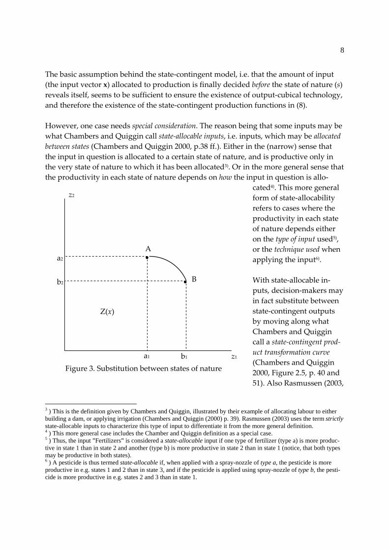
The basic assumption behind the state‐contingent model, i.e. that the amount of input (the input vector x) allocated to production is finally decided before the state of nature (s) reveals itself, seems to be sufficient to ensure the existence of output‐cubical technology, and therefore the existence of the state‐contingent production functions in (8). However, one case needs special consideration. The reason being that some inputs may be what Chambers and Quiggin call state‐allocable inputs, i.e. inputs, which may be allocated between states (Chambers and Quiggin 2000, p.38 ff.). Either in the (narrow) sense that the input in question is allocated to a certain state of nature, and is productive only in the very state of nature to which it has been allocated3). Or in the more general sense that the productivity in each state of nature depends on how the input in question is allo‐

cated4). This more general form of state‐allocability refers to cases where the productivity in each state of nature depends either on the type of input used5), or the technique used when applying the input6). With state‐allocable in‐puts, decision‐makers may in fact substitute between state‐contingent outputs by moving along what Chambers and Quiggin call a state‐contingent prod‐uct transformation curve (Chambers and Quiggin 2000, Figure 2.5, p. 40 and 51). Also Rasmussen (2003,

3 ) This is the definition given by Chambers and Quiggin, illustrated by their example of allocating labour to either building a dam, or applying irrigation (Chambers and Quiggin (2000) p. 39). Rasmussen (2003) uses the term strictly state-allocable inputs to characterize this type of input to differentiate it from the more general definition. 4 ) This more general case includes the Chamber and Quiggin definition as a special case. 5 ) Thus, the input ”Fertilizers” is considered a state-allocable input if one type of fertilizer (type a) is more produc-tive in state 1 than in state 2 and another (type b) is more productive in state 2 than in state 1 (notice, that both types may be productive in both states). 6 ) A pesticide is thus termed state-allocable if, when applied with a spray-nozzle of type a, the pesticide is more productive in e.g. states 1 and 2 than in state 3, and if the pesticide is applied using spray-nozzle of type b, the pesti-cide is more productive in e.g. states 2 and 3 than in state 1.

•

•

z1b1a1

b2

a2

z2

A

B

Z(x)

Figure 3. Substitution between states of nature

9

Figure 6) derives a product transformation curve illustrated as a continuous decreasing concave function in the z1‐z2 plane, similar to the curve AB in Figure 3 (this paper). This type of substitutability may be included in the model described so far, by expand‐ing the input vector. Assume for instance that input xj is a state‐allocable input, and that there are S different types of input j or S different techniques for applying input j. Then instead of xj, define new input variables xj1, …, xjS, where xjs is the amount of input j allo‐cated to state s (s=1,…, S). Using these new variables as decision variables instead of just xj, provides the opportu‐nity to move along the state‐contingent product transformation curve. Figure 3 illus‐trates a case where, when all the input (x=xj) is allocated to state 2 (xj2=xj, xj1=0), the state‐contingent output is A (a1 in the case of state s=1, and a2 in the case of state s=2) and where, when all the input x is allocated to state 1 (xj1=xj, xj2=0), the state‐contingent out‐put is B (b1 in the case of state s=1, and b2 in the case of state s=2). Combinations of xj1>0 and xj2>0 yield state‐contingent output somewhere along the curve between A and B. However, this way of combining different amounts of state‐allocable input is not in real‐ity different from combining different amounts of all other inputs. The conclusion is that output‐cubical technology covers the production technology un‐der uncertainty. In the case of some inputs being state‐allocable input, then the vector of decision variables should be expanded so that the amount of input allocated to a specific state of nature is considered an individual decision variable (input). In that case, the general model framework of the output‐cubical technology illustrated in Figure 2 holds. The Lagrangean is therefore:

01

1 1( ,..., ) ( , ) ( ) ( )

S nF

S s s s N N i is i

L W q q H z x x w x Cµ γ δ= =

= − − − − −∑ ∑x (9)

Differentiating (9) with respect to xi, (i = 1,..., N) yields the following first order condi‐tions:

1 1

0S S

ti t i

s ts i

fWw wq x

µ δ= =

∂∂− + − ≤

∂ ∂∑ ∑ (i = 1,..., n) (10a)

10

1 1

( ) 0S S

ti t i i

s ts i

fWw w xq x

µ δ= =

∂∂− + − =

∂ ∂∑ ∑ (i = 1,..., n) (10b)

1

0S

tt

t N

fx

µ γ=

∂− ≤

∂∑ (11a)

1

( ) 0S

tt N

t N

f xx

µ γ=

∂− =

∂∑ (11b)

Assuming an interior solution ( *

ix > 0) and therefore an equal sign in (10a), the conditions in (10) may be expressed as:

1

1

st

tti iS

tjt

t j

fw x

fwx

µ

µ

=

=

∂∂

=∂∂

∑

∑ (i, j = 1,..., n) (12)

where t jf x∂ ∂ is the marginal product of input j in state t (MPPjt). Differentiating (9) with respect to zs, (s = 1,..., S) yields the following first order condi‐tions:

0s ss

Wpq

µ∂− ≤

∂ (s = 1,..., S) (13a)

( ) 0s s ss

Wp zq

µ∂− =

∂ (s = 1,..., S) (13b)

Assuming interior solutions ( *

sz >0) and therefore an equal sign in (13a) implies:

s ss

Wpq

µ ∂=

∂ (14)

Inserting (14) in (12) yields:

11

1 1

1 1

S St

t tit ti t i tS S

tjt tj

t tt j t

fW Wp VMPw q x q

fW Ww p VMPq x q

= =

= =

∂∂ ∂∂ ∂ ∂

= =∂∂ ∂

∂ ∂ ∂

∑ ∑

∑ ∑ (i, j = 1,..., n) (15)

where VMPti is ( / )t t ip f x∂ ∂ i.e. the Value of Marginal Product of input xj in state t. If one assumes risk neutrality, then (15) reduces to:

( )( )

i i

j j

w E VMPw E VMP

= (i, j = 1,..., n) (16)

which expresses that for optimal production, the risk‐neutral decision maker should combine variable input in such a way that the relation between the expected marginal products is equal to the relation between prices. Using (14) in (10a), assuming an interior solution and therefore an equal sign, the condi‐tion for optimal production in (10) may also be expressed as:

1 1

( )S S

tt i

t tt i t

fW Wp wq x q

δ= =

∂∂ ∂= +

∂ ∂ ∂∑ ∑ (i = 1,..., n) (17)

which under risk‐neutrality reduces to: ( ) (1 )i iE VMP w δ= + (i = 1,..., n) (18) (18) shows that a risk neutral decision maker should add variable input, as long as the expected value of the marginal product is higher than the input price (adjusted for any budgetary restriction) Assuming interior solutions in both (11a) ( *

Nx >0) and (13a) ( *sz >0), the two conditions

may be combined, yielding the following condition for optimal use of fixed input:

1

St

tt t N

fWpq x

γ=

∂∂=

∂ ∂∑ (19)

Under risk‐neutrality (19) reduces to: γ=)( NVMPE (20)

12

which tediously expresses that a risk‐neutral decision‐maker should apply fixed input, as long as the expected value is higher than the shadow price. If the fixed input is state‐allocable, in order for it to be allocated to different states of na‐ture, then, as mentioned previously, the input vector x is expanded from (x1, …, xn, xN) to (x1, …, xn, xN1, …, xNS), where xNt (t=1,…, S) is the amount of fixed input xN allocated to state t. The restriction (4) (with only one output (M=1) and one fixed input xN) is ad‐justed correspondingly, so that in this case:

1

0S

FNs N

sx x

=

− ≤∑ (21)

indicating that the amount of fixed input allocated to the different states of nature, may not exceed the amount of input available. Including these alterations in the model, the conditions (19) and (20) change to:

1

St

tt t Ns

fWpq x

γ=

∂∂=

∂ ∂∑ (s = 1,…, S) (22)

Under risk‐neutrality (22) reduces to: ( )NsE VMP γ= (s = 1,…, S) (23) Thus, fixed state‐allocable input (input, which may be allocated to specific states of na‐ture) should be allocated between states of nature, so that the expected values of the marginal products are equalized across states. The result of optimizing production, as derived in (9) – (23), is illustrated in Figure 4 for S=2. Origo of the system of coordinates in Figure 4 corresponds to ks‐cF (s=1,…, S) in Fig‐ure 1, so that the axes in Figure 4 measure changes in income compared to the no produc‐tion alternative illustrated in Figure 1. Thus, the net‐returns ys are estimated as (compare with (2)):

1 1

S n

s s s i is i

y z p w x= =

= −∑ ∑ (s=1,…, S) (24)

13

and the optimal produc‐tion plan is the state‐contingent net‐returns ( *

1y , *2y ) in Figure 4.

According to the assump‐tions made earlier, the net return set Y(xN,C0) in Fig‐ure 4 (the y’th below the curve bb) is determined by the amount of fixed input (xN) and the budget (C0). To interpret the net‐return curve bb in Figure 4, com‐pare with the net‐return curve derived in Rasmus‐sen (2003)7) for the one‐

variable‐input case. In Figure 5, two such one‐variable‐input net return curves are illustrated with an increasing amount of one variable input in the direc‐tion of the arrow, assuming that all other inputs are fixed. The two curves represent dif‐ferent amounts of fixed input. The net return curve bb may now be interpreted as the enve‐lope curve for all possible one‐variable‐input curves, of which only two are shown in Figure 5. Thus, the implicit assumption behind the net return possibil‐ity curve bb is that all inputs

7 ) See Rasmussen 2003, Figure 7 and 8 pp. 466-467

b

y1*

y2*

45°

W(y)=w*

y1

y2

b Figure 4. Optimal state‐contingent income

Indifference curve

Y(xN,C0)

•

•

y2

b

bNet return curves ‐ one variable input

Net return curves ‐ all inputs except xN variable

45°

y1

Figure 5. Derivation of net return curve

14

are used efficiently.

3. Empirical application The criteria for optimal production derived for risk‐averse decision‐makers (equations (17) and (22)) involve, not only the derivatives of the state‐contingent production func‐tions, but also the derivatives of the state‐contingent utility function. To implement the criteria derived, i.e. to use the criteria in decision making contexts or to perform com‐parative static analysis, one therefore needs to know the state‐contingent production functions, the state‐contingent output prices8), and the utility function. Elicitation of the utility function has historically been one of the major problems encoun‐tered in the application of the Expected Utility model (EU‐model)9). However, the state‐contingent approach does not provide any immediate shortcuts with respect to the de‐

mand for identifying risk preferences. And while the endeavours in the literature have focussed on elicitation of von Neumann‐Morgen‐stern (NM) utility func‐tions, the more general preference structure on which the state‐contingent approach is based, may even involve further chal‐lenges. However, there are cases in which empirical applica‐tion is possible without ex‐plicit knowledge of the util‐ity function. Such cases ex‐ist if there are what Hirshleifer and Riley call Complete Contingent Mar‐

8 ) To simplify, only production uncertainty (and not price uncertainty) is explicitly considered in the following. 9 ) (Moschini and Hennessy 2001) give a good review of the published research on identifying risk preferences (the NM-utility function) in the EU-model context.

y1*

y2*

Figure 6. Separation of production and consumption.

y2

Slope τ1/τ2

y1c1

c2

45°

Indifference curve

15

kets (CCM), i.e. markets for direct trading in state‐contingent claims (for instance mar‐kets for insurances), or Complete Asset Markets (CAM), i.e. markets for assets, includ‐ing e.g. financial assets (loans, futures, options, etc.), which may be used to re‐allocate state‐contingent incomes (Hirshleifer and Riley 1992). If such markets (and therefore prices of state‐contingent incomes) exist, then it is possi‐ble to separate the production decision and the consumption decision (Hirshleifer and Riley 1992). The procedure for optimizing production is in this case, to substitute the de‐rivatives of the utility function ( sW y∂ ∂ , s=1,…, S) in (17) and (22) with the relative prices of state‐contingent income directly available as market prices (CCM) or indirectly estimated (CAM). The procedure is illustrated in Figure 6, which corresponds to Figure 4, shown earlier. The relative prices of state‐contingent incomes are τ1/τ2, and the optimal production therefore provides the net‐return ( *

1y , *2y ). This implies a production plan with higher

net‐return in state 2 and less net‐return in state 1 compared to Figure 4. The optimal state‐contingent consumption after trading in the market for state‐contingent claims at prices τ1/τ2 is (c1, c2). (Compare to Hirshleifer and Riley, 1992, Figure 2.5, p. 56). Although this approach will not be discussed further here, it is without a doubt an ap‐proach of increasing importance (Coble and Knight 2002; Allen and Lueck 2002; Pannell et al. 2000; Chambers and Quiggin 2002a; Babcock and Hennessy 1996; Quiggin 2002; Chambers and Quiggin 2000). As a basis for empirical work, the approach using direct or indirect markets for state‐contingent claims, seems much more promising than using effort to elicitate the decision‐makers’ utility function. In the ideal case of insurable mar‐kets and actuarially fair insurance contracts, the problem of optimizing production in reality boils down to the problem of identifying the production plan that maximizes the expected net‐return (Nelson and Loehman 1987). Further, the state‐contingent approach is very well suited to this, as indicated by the illustration in Figure 6. As the objective of this paper is to compare the state‐contingent approach with the em‐pirical approaches typically taken in the EU‐model context (Hardaker et al. 1997), the following analysis will be based on the direct approach, i.e. without considering markets for state‐contingent claims. In this case, empirical application involves choosing/estima‐ting an appropriate utility function. In the following, the EU‐model and the more general model based on the state‐contingent approach will be compared, and the problems related to empirical applica‐tion will be discussed. The problems relating to the choice of utility function are dis‐

16

cussed in the first subsection. In the next subsection, problems connected to describing the production technology are discussed.

3.1. Choice of Utility Function.

3.1.1. The EU-model The popular choice of functional form of the NM utility function in the EU model framework is the negative exponential:

( ) 1 yv y e λ−= − (25) where λ (λ >0) is the Arrow‐Pratt coefficient of absolute risk aversion, i.e. λ = ‐v’’(y)/v’(y). Although this form implies the assumption of constant absolute risk aversion (CARA) which is not usually regarded as a desirable property (Hardaker et al. 1997), it has found extensive use in applied analyses of decision making under risk (Allen and Lueck 2002; Pope and Just 1991; Chavas and Holt 1990; Smith et al. 2003) due to its mathematical/analytical properties: If y is normally distributed, then the expected utility is a simple function of expected value (E) and Variance (V):

( ) ( ) ( )2

W E y V yλ= −y (26)

More desirable functional forms are the logarithmic: ( ) ln( )v y y= (27) which has decreasing absolute risk aversion (DARA), and the power function:

(1 )1( )1

rv y yr

−=−

(28)

where r is the Arrow‐Pratt coefficient of relative risk aversion, i.e. r = yλ . Like the loga‐rithmic, the power function also has decreasing absolute risk aversion (DARA) and con‐stant relative risk aversion (CRRA). For r = 1, the power function (28) reduces to the logarithmic (27). Also, the quadratic function:

17

2( )v y y by= − (29) has been rather popular (b>0), because it implies an EV utility function, i.e.:

2( ) ( ) ( ) [ ( )]W E y hV y h E y= − −y (30) The properties of the different types of utility functions may be illustrated by deriving the rate of substitution in utility of ys for yt (RSUst), defined as the slope dys/dyt of an iso‐utility curve in state‐space10). Thus, a utility function W(y) based on the NM‐utility func‐tion in (25) has the following property:

( )RSU s ty ys sst

tt

Wy eWy

λππ

− −

∂∂

≡ =∂

∂ (31)

A utility function based on the NM‐utility function (27) has the following property:

RSU s s tst

t st

Wy y

W yy

ππ

∂∂

≡ =∂

∂ (32)

Finally, a utility function based on (28) has the following property:

RSUr

s s tst

t st

Wy y

W yy

ππ

∂⎛ ⎞∂

≡ = ⎜ ⎟∂ ⎝ ⎠∂ (33)

It follows from (31), (32), and (33) that the marginal rate of substitution (i.e. the amount of income in state s that would substitute one unit of income in state t) increases, the greater the difference in income in the two states of nature is. Further, it follows directly from (32) and (33) that the marginal rate of substitution in EU‐models, based on the logarithmic and power functions, does not change when income in all states are multi‐plied by a constant (CRRA). A consequence of (31) is that the marginal rate of substitu‐tion for exponential function does not change when income in all states is allotted a con‐stant (CARA).

10 ) See (Dillon and Anderson 1990) p. 125 who use this term to describe the slope in EV-space.

18

3.1.2. The general (state-contingent) form In the state‐contingent framework, utility functions based on the EU‐model may still be applied (Expected Utility is just a special form of the more general utility function). However, it is appropriate to consider more general functional forms. In this context, one needs to consider what restrictions to place on the utility function. The most common restriction to place on preferences is that the decision maker is risk‐neutral or has risk‐aversion. This is the case where the utility function is quasi‐concave over stochastic incomes. (Utility functions based on the Neumann‐Morgenstern utility functions mentioned in the previous section all fulfil this restriction). In the general case of the state‐contingent framework, preferences only depend on the state‐contingent outcomes, and not explicitly on the probabilities as is the case in the EU‐model. Besides the linear utility function (in which case the utility is simply the expected value of net‐returns), the simplest functional form describing risk‐averse decision makers in the state‐contingent framework, is the Cobb‐Douglas:

01

( ) t

Sat

t

W a y=

= ∏y (34)

with 0<at<1 to ensure that the function is quasi‐concave. The fact that the relative probabilities are given as the slope of the indifference curve along the bisector (Chambers and Quiggin 2000), i.e.:

1 S

s s

tt y y y

Wy

Wy

ππ

= = =

∂∂

=∂

∂L

( , )s t∈Ω (35)

implies, that with a Cobb‐Douglas utility function, the relative probabilities are deter‐mined as:

s s

t t

aa

ππ

= ( , )s t∈Ω (36)

19

Thus, the choice of the parameters of the Cobb‐Douglas utility function (at, t=1,…, S) is at the same time a choice of the relative (subjective) probabilities implicitly attached to the different states of nature. On the other hand, if the probabilities sπ (s = 1,…, S) have al‐ready been determined, then the relative value of the parameters as (s = 1,…, S) are de‐termined by (36). A Cobb‐Douglas utility function has the derivative:

( )s

s s

aW Wy y

∂=

∂y ( )s∈Ω (37)

and therefore the RSUst is:

RSU s s tst

t st

Wy y

W yy

ππ

∂∂

≡ =∂

∂ (38)

Comparing (38) with (32), one sees that a Cobb‐Douglas utility function provides the same marginal rate of substitution (slope of the indifference curve) as an EU utility func‐tion, based on the logarithmic form (27) of the NM utility function. Equation (38) also shows that the Cobb‐Douglas utility function implies constant rela‐tive risk aversion (CRRA) (the expansion path is a straight line through origo) and there‐fore decreasing absolute risk aversion (DARA), which according to Meyer (Meyer 2002) is a very acceptable assumption. However, the Cobb‐Douglas function is different from the EU model, in the sense that the marginal utility of income in state s (see (37)) not only depends on the relative prob‐ability of state s (as) and of the net‐return in state s (ys), but also on the net‐return in the other states of nature (W(y)). In this sense, even the relatively simple Cobb‐Douglas functional form potentially provides more flexibility in the description of preferences, than the utility functions based on the popular forms of NM utility functions, mentioned in the previous section. An even more flexible functional form is the translog:

20

01 1 1

ln ( ) ln ln ½ ln lnS S S

t t st s tt s t

W a a y b y y= = =

= + +∑ ∑∑y (39)

Notice that the Cobb‐Douglas utility function is a special case of the translog utility function (bst = 0 (all s, t)). A translog utility function has the following properties (Boisvert 1982):

1

( ) ( ( ln ))S

s st tts s

W W a b yy y =

∂= +

∂ ∑y (40)

and therefore:

1

1

ln

ln

S

s st ts t t

Ss

t ts stt

W a b yy y

W y a b yy

=

=

⎛ ⎞∂ +⎜ ⎟∂ ⎜ ⎟=∂ ⎜ ⎟+∂ ⎜ ⎟

⎝ ⎠

∑

∑ (41)

As the translog is a relatively general form, one cannot expect it to be well‐behaved globally (non‐decreasing, quasi‐concave, and constant relations between probabilities (i.e. (35)), unless certain restrictions are employed. To make sure that W is non‐decreasing, (40) has to be nonnegative, i.e.:

1

( ln )S

s st tt

a b y=

≥ − ∑ (s = 1,…, S) (42)

To ensure quasi‐concavity the Bordered Hessian matrix should be negative definite. The translog function is homothetic if and only if:

1

0S

stt

b=

=∑ (s = 1,…, S) (43)

Thus, (43) becomes the condition that the translog utility function in question has CRRA. Using (35), the following relation exists between the parameters and the probabilities:

21

1

1

ln

ln

S

s sts t

St

t tst

a y b

a y b

ππ

=

=

+=

+

∑

∑ (s, t= 1,…, S) (44)

This condition (44) must be valid for any value of y. This is the case only when:

0Fk

∂=

∂ (45)

where

1

1

ln( )

ln( )

S

s sttS

t tst

a ky bF

a ky b

=

=

+≡

+

∑

∑ (k>0; s, t= 1,…, S)) (46)

Condition (45) applies only if:

1 1

S S

t st s tst s

a b a b= =

=∑ ∑ (s, t= 1,…, S) (47)

This restriction (47) ‐ together with the restriction (42) and the condition that the Bordered Hes‐sian is negative definite ‐ thus becomes the general restriction on the translog function to be con‐sidered a state‐contingent utility function. If the condition (47) is replaced by (43), then the translog utility function is a CRRA utility function. Risk aversion is ensured when W is quasi‐concave. If the translog is homothetic (fulfils (43)), then according to (44) the relation between probabilities is:

s s

t t

aa

ππ

= ( , )s t∈Ω (48)

which is the same as for the Cobb‐Douglas function. This means, that if one chooses a translog functional form of the utility function, concurrently introducing the condition that the utility function has CRRA, then the relative probabilities determine the relation between the a‐parameters as shown in (48).

22

To summarize, a Cobb‐Douglas utility function in state‐contingent income measures, yields a utility function with the same degree of flexibility in the state‐contingent world as a logarithmic von Neumann‐Morgenstern utility function in the Expected Utility world. More flexible functional form is for instance the translog, which has proven suc‐cessful in other contexts. But even the flexibility of the translog is limited when one con‐siders the restrictions necessarily placed on state‐contingent utility functions.

3.2. The Production Technology Although the basic problems of optimising production under uncertainty are the same, the expected utility model (the EU‐model) and the state‐contingent model are based on different approaches in describing the technology. While the EU‐approach focuses on the stochastic production function and estimation of probability distributions of yield (and prices), the state‐contingent approach focuses on state‐contingent production functions, and therefore yields (and prices) contingent on discrete states of nature. Just (Just 2003) compares the EU‐model and the state‐contingent model (p. 140). He states that the relative advantage of the two approaches depends on how many mo‐ments of the probability distribution it is necessary to estimate, compared to the number of states of nature. He claims that if there are many states of nature, then the state‐contingent approach is disadvantaged and that “…most distributions facing farmers have large numbers of potential outcomes (states of nature)” (p.140). For example, most yield and price distributions have a large number of outcomes. In fact, depending on the units used for measuring yields and prices, there may even be thousands of yields and prices, and therefore the same huge number of states to consider. Although at first sight this point seems important, it also exposes the mistakes one may make if the differences between the two approaches are not carefully considered. While the EU‐model typically focuses on the probability distributions of yields and prices, i.e. the consequences of the uncertain environment, the state‐contingent approach focuses di‐rectly on the uncertain environment, i.e. the states of nature. Thus, yields and prices are not (as indicated by Just) “states of nature”, but rather consequences of “states of nature”, (e.g. in the case of crop production consequences of the amount of rain or hours of sun‐shine). In a decision making context, the state‐contingent approach is much more ap‐propriate, because it makes explicit that the realized yield of a crop of wheat is a conse‐quence, not only of the controllable inputs (the input vector x), but also of the interaction with the non‐controllable inputs, i.e. the “states of nature” (amount of rain, hours of sunshine, etc.).

23

However, it is not obvious how one should empirically approach the problem of facing maybe thousands of discrete states of nature and the demand of estimating, for each of these states of nature, a state‐contingent production function usable within the theoreti‐cal framework afterwards, as presented in Section 2. As will be shown in the following, it may not be a question of choosing either the EU‐model based on the stochastic production function or the state‐contingent model based on state‐contingent production functions. In an empirical context, it may be a question of combining the two approaches. In the following, the focus will be primarily on the state‐contingent production function. The EU approach based on the stochastic production function is well known in the lit‐erature, and will only be briefly mentioned in the first section to provide comparisons with the state‐contingent production function mentioned later.

3.2.1. The stochastic production function The EU‐model is typically based on what Chambers and Quiggin (Chambers and Quig‐gin 2002b) call Stochastic Production Functions, i.e. functions of the type: ( , )t tz f ε= x (49) for instance of the form: Additive: ( )t tz f ε= +x (50) Multiplicative: ( )t tz f ε= x (51)

Just‐Pope: ( ) ( )t tz g h ε= +x x (52) The empirical problem is related to estimating the functions and the probability density function of the error term εt, or at least the first two or three moments11). The Just‐Pope production function form in (52) (Just and Pope 1978) has proven to be especially popu‐

11 ) In the EU approach, much energy is used in choosing a type of distribution (Normal, beta, etc) and estimating the parameters, typically the expected value and the variance (Dillon and Anderson 1990; Goodwin and Ker 2002).

24

lar in applied analyses (Moschini and Hennessy 2001), and has been used by for instance (Larson et al. 2002; Smith et al. 2003) and (Horowitz and Lichtenberg 1994)12).

3.2.2. The state-contingent production function With the state‐contingent model, one of the immediate problems one faces in applied work is how to define the possible states of nature. In theory, a state of nature is formally defined as a complete description of the external condi‐tions (the environment) in the sense that, given a specific state of nature (non‐controllable inputs) and a production decision (amount of controllable inputs), then the consequences (outputs or prices) are uniquely determined. A state may be quantified by a vector of state‐variables describing the state‐space using quantitative variables such as temperature, amount of sunshine, amount of rain, etc. While in theory one can easily imagine a state description being complete in the sense that everything relevant has been described/registered, this is typically not the case when it comes to empirical application. In practice, it is often impossible to make a com‐plete description/registration of a state of nature. Either because one does not know all the state‐variables influencing output, or because the true level of the state‐variables is uncertain. In both cases the state description is incomplete, and the state‐contingent out‐put (the output given a specific registered13) state of nature) is a stochastic variable. Consider first the case where the complete state space is the set Ω = 1,…, S. To proceed with the state‐contingent approach based on the theory developed in Section 2, one needs estimates of the state‐contingent production function for each of the S states of na‐ture. Thus, in the ideal case where the state description is complete, the applied re‐searcher has available the following S state‐contingent production functions: ( )s sz f= x (s = 1,…, S) (53) either in the form of mathematical functions, or in the discrete form as numbers in a ta‐ble.

12 ) For further introduction to the approach in the EU-model, see for instance (Dillon and Anderson 1990) 13 ) I use the term registered state to describe the way in which a state is actually (empirically) registered. If not all relevant state-variables are registered or if the registered level of the individual state-variables is uncertain, then the state description is incomplete. A real state is the actual state, which exists independently of being registered or not. In the following when I use the term state, I mean registered state unless explicitly stated.

25

In practice this ideal situation rarely exists. First of all, the number of possible real states (S) is often very large. (This is indeed the case when the variables describing the states of nature, are continuous variables). Therefore, if state‐contingent production functions are available, it will in practice typically be for only some of the possible real states. To illustrate, consider the simple decision problem of fertilizer application to a crop of barley. The yield of barley four months later de‐pends both on the amount of fertilizer applied now, but also on the real state of nature during the growing season. Assume for simplicity that the real state of nature may be quantified by the amount of sunshine and rain during the growing season. Further as‐sume that the relevant interval of possible amount of rainfall is between 10 and 50 cen‐timetres, and that the relevant interval of the amount of sunshine is between 200 and 800 hours. With only these two state‐variables describing the real states of nature, there would – if state‐variables are measured in integer units ‐ be 50x600 = 24,000 different states of nature. Imagine that state‐contingent production functions are estimated based on experimental yields. Then, even in the unrealistic case that none of the states came out twice, it would take at least 24,000 years to collect enough observations to estimate the 24,000 state‐contingent production functions! Secondly, if state‐contingent production functions are in fact available, then they are probably only estimates of the true state‐contingent production functions, so that the output zs is a stochastic variable: ( , )s s sz f ε= x ( Es∈Ω ) (54) where εs is a stochastic error term given state s, and EΩ is the set of states for which pro‐duction functions have been estimated. A state of nature is often characterized by a large number of state‐variables. If only a few of these variables are in fact observed/registered when doing the experiments on which the state‐contingent production function is based, then the state‐description is incomplete. The variables registered could be e.g. monthly rainfall and hours of sunshine/month. However, all the other variables influ‐encing the output, may not be observed. These other variables could for instance be wind velocity or CO2 content of the atmosphere as well as many other variables influ‐encing production. Therefore, even if one were so lucky to replicate production under the (apparently) same conditions (the same amount of rainfall and the same amount of sunshine), one cannot be sure of achieving the same production result (with the same amount of controllable input), because the other (non‐controllable) variables may con‐tain alternative values. For this very reason, the state‐contingent production for a spe‐

26

cific state of nature, (i.e. for a specific registered state of nature, for instance a hours of sunshine and b centimetres of rain) would be a stochastic variable as indicated in (54), because the state‐description is incomplete. Thus, the typical situation facing the applied researcher is that if state‐contingent pro‐duction functions are available at all, it is probably only for a few of the possible real states of nature. And for those real states for which they are available, the state‐description is probably incomplete, i.e. has the general form of a stochastic production function shown in (54). This indeed is the main obstacle to applying the state‐contingent approach in an empirical/nor‐mative context. Experimental data and farm response data typically do not provide the information necessary to estimate state‐contingent production functions. The question is therefore, how the possible advantages of the state‐contingent approach may be used when the data necessary to support the approach are often not available. To illustrate the problem and a possible procedure to deal with it, consider the following simple example.

A real state of nature is completely quantified by the level of four state‐variables a1, a2, a3 and a4 (in crop production this could be for instance the amount of rain, the amount of sunshine, concentration of CO2 in the atmosphere, and wind veloc‐ity). Assume for simplicity that there are 10 possible levels of the first state vari‐able a1 and 3 possible levels of each of the other three state‐variables a2, a3 and a4. If any combination is possible, there would therefore be 10×3×3×3=270 possible real states of nature (S = 270). The probabilities connected to each of these possi‐ble states may or may not be known. Assume further that for one reason or another, only the first state‐variable (a1) is systematically being registered when performing the experiments on which esti‐mation of production functions are based. Thus, the states registered refer to the 10 possible levels of state‐variable a1. Finally, assume that production functions have been estimated for only 4 of these 10 possible states, so that of the 10 possi‐ble state‐contingent production functions f1(x),…, f10(x), only f2(x), f5(x), f6(x), and f8(x) are in fact available. Therefore, the information available as a basis for deci‐sion making are the 4 state‐contingent production functions and the knowledge of the possibility that nature may take one of 270 states of nature and the corre‐sponding probabilities.

27

Consider first the 4 state‐contingent production functions available. The fact that the level of the other 3 state variables a2, a3 and a4 were not registered when the state‐contingent production functions were estimated, means that the production in each of the four registered states is a stochastic variable, i.e.: ( , )s s sz f γ= x (s = 2, 5, 6, 8) (55) where sγ are state‐specific error terms drawn from state‐contingent probability distributions that are determined by the variability of other three state‐variables that are not registered. Assume that the probability distribution of each of the four error terms sγ (s=2, 5, 6, 8) are known (have been estimated). Then the four (state‐contingent), stochastic production functions in (55) are, in principle, a description of the technology for 4/10 of the 270 real states, i.e. for the 108 real states. But what about the technology for the remaining 270‐108 = 162 states? In principle, nothing is at this stage known about the technology for these re‐maining 162 states. One way to proceed is to consider each of the estimated state‐contingent produc‐tion functions fs(x) ( Es∈Ω ) as being representative of (being an estimate of) – not only state s, but also of all possible states of nature in the vicinity of state s. In the present example, this means that f2() is considered representative also of state 1 and 3, that f5() is considered representative also of state 4, that f6() is considered representative also of state 7, and that f8() is considered representative also of states 9 and 10. In this way, the four available production functions are used as estimators of the remaining (unknown) production functions. Obviously this way of estimating the technology for the remaining 6 states, adds another error term, so that in this case: ( , , )s s s sz f γ η= x (s = 1, 3, 4, 7, 9, 10) (56) where sη is an error term with a probability distribution which depends on how much two nearby states in the a1‐dimension resembles each other.

28

The example illustrates first of all the extreme data requirements necessary to apply the state‐contingent approach in its “pure” form. Secondly, it proposes what can be done in the typical second best situation with incomplete date. Finally, it shows that in the real world situation, it is not a matter of choosing between the state‐contingent production function and the stochastic production function. It is rather a matter of combining the two. The example also provides the foundation for describing the relationship between the state‐contingent production function and the stochastic production function. The two ways of describing the technology are just special cases of the more general description of the technology in (54). In the special case that EΩ = Ω (production functions have been estimated for all possible states), then the error term in (54) vanishes, and the technology description is in the form of (non‐stochactic) state‐contingent production functions as in (53). In the special case that EΩ =∅ (available production functions refer to no specific state), then the model (54) reduces to the (pure) stochastic production function in (49).

4. Example In this paper the focus has been on the empirical application of the state‐contingent ap‐proach. It is therefore appropriate to close the paper, demonstrating the application of the state‐contingent theory. The demonstration is based on the following relatively sim‐ple production example14). An output z is produced according to the following two state‐contingent production functions available:

0.6 0.2 0.11 1 2 3[ ] 3E z x x x= in state s=1 (57.1)

0.2 0.4 0.3

2 1 2 3[ ] 2.5E z x x x= in state s=2. (57.2) where E[zs] is the expected production in state s.

14 ) Although the demonstration is based on a simple text book example, it reveals both the demand for data and the potential strength of the state-contingent approach

29

Input prices are exogenous with the following prices of the three variable inputs x1, x2 and x3: w1 = 10 w2 = 4 (58) w3 = 1.5 Expected output prices are also exogenous and there is no price uncertainty, i.e. the out‐put price is the same in states 1 and 2: p1 = 10 p2 = 10 Further, the (subjective) probabilities of states 1 and 2 are, respectively: 1π = 0.625 2π = 0.375 Finally, there is no fixed cost and there is no income from other sources, i.e. cF = 0 k1 = 0 k2 = 0 Therefore, net‐income qs in state s is the same as net‐return ys in state s. Notice that al‐though the output prices are here assumed to be the same in both states, this need not always be the case. However, to interpret the results, only production uncertainty is considered. To illustrate the consequences of uncertainty, consider first the case of certainty (perfect information). In the case of perfect information, the decision‐maker always knows in advance what state of nature will emerge, and is therefore able to adjust the amount of input to the actual state of nature. In the case of certainty, the objective is to maximize net‐income, i.e. the value of output minus variable costs. In state 1 optimization is based on the state‐contingent production function (57.1) and in the case of state 2, the optimization is based on the state‐contingent production function (57.2). The result of optimizing15) production in the cer‐tainty case is shown in the first part of Table 1.

15 ) All optimizations were carried out using the solver CONOPT3 in GAMS (GAMS Development Corporation 2003)

30

Table 1. Optimization of production under uncertainty. An example

Input x1 Units

Input x2 Units

Input x3 Units

Output Units

Net‐return ys ($)

CERTAINTY ‐ State 1 275 230 306 459 459 ‐ State 2 610 3,052 6,104 3,052 3,052 (Average) (401) (1,288) (2,480) (1,431) UNCERTAINTY Risk‐neutral 170 272 466 388 388 ‐ State 1 371 222 ‐ State 2 415 664 Risk‐averse A 175 237 389 366 376 ‐ State 1 360 322 ‐ State 2 375 466 Risk‐averse B 171 253 425 375 385 ‐ State 1 364 276 ‐ State 2 393 566 The first row of the table shows the optimal amounts of the three variable inputs to be used in the case of state 1. The optimal production is 459 units of output z1, and the net‐return (y1) is $459. The second row shows the corresponding information in the case of state 2. In the case of state 2, it pays to apply much more input than in state 1. Especially the amount of the (cheap) input x3 is increased, because in state 2 this input x3 is much more productive than in state 1. The production is about 7 times higher (3,052/459) in state 2 than in state 1. The third row of the table shows the long term use of input and net‐return in the case of certainty. The results are estimated by weighing the data in the first two rows by the frequencies of the two states of nature (i.e. 0.625 and 0.375, respectively) In the case of uncertainty, a risk‐neutral decision‐maker applies input according to the crite‐rion (18), i.e. E(VMPi) = wi (no budget limitation). The results of optimising production using this criterion are shown in the three rows under the heading “Risk‐neutral” in Ta‐ble 1. Thus, in the case of uncertainty, a risk‐neutral decision‐maker will apply 170 units x1, 272 units of x2, and 466 units of x3. The expected output is 388 units of z (371 units in the case of state 1, and 415 units in the case of state 2), and the expected net‐return is $388 ($222 in state 1 and $664 in state 2).

31

Now, assume that the decision maker is risk‐averse and has a Cobb‐Douglas utility func‐tion. As the probabilities are already given in the beginning, the functional form is: 0.625 0.375

1 2 1 2( , ) h hW q q Aq q= (59) where A and h are parameters (A>0, 0<h<1.6). The arguments q1 and q2 are expected net‐income in states 1 and 2, respectively. Arbitrarily, choose h=0.8. Further, to identify which of the two states is “good” state, and which is the “bad” state (Rasmussen, 2003), the utility function in (59) is scaled so that the sum of the partial derivatives is 1 for the value x chosen by a risk‐ neutral decision maker. Calculating the sum of the derivatives of: 0.5 0.3

1 2 1 2( ( ), ( )) ( ( )) ( ( ))n n n nW q q A q q= × ×x x x x (60) where xn is the input vector for risk‐neutral decision‐maker, and where therefore the values of q1 and q2 ‐ according to Table 1 ‐ are 222 and 664, respectively, and setting this sum equal to 1, yields the value A = 3.53. Using this value of A in (60) yields 1W q∂ ∂ = 0.832 > 0.625 = 1π and 2W q∂ ∂ = 0.167 < 0.375 = 2π . Therefore, according to Rasmussen, 2003, state 1 is a “bad” state of nature, and state 2 is a “good” state of nature. Thus, receiving one more dollar in state 1 would pro‐vide more utility than the probability of this state of nature, and vice versa with state 2. When the decision‐maker is risk‐averse, the criterion for optimizing is given earlier in con‐dition (17). Applying this condition to a decision‐maker with a utility function as in (59) with h=0.8 and A=3.53, yields the production plan shown in the three rows under the heading “Risk‐averse A” in Table 1. As one would expect, the optimal production is lower for a risk‐averse decision‐maker than for a risk‐neutral decision maker. As risk‐neutral decision‐maker produces an ex‐pected output of 388 units of z, while a risk‐averse decision‐maker produces an expected output of 366 units. However, what is more interesting is that the risk‐averse decision‐maker uses input in another combination than the risk‐neutral decision‐maker. Notice especially that while a risk‐averse decision‐maker reduces input x2 and x3 compared to a risk‐neutral decision‐maker, the use of input x1 is increased (from 170 to 175 units). The reason being that in this example, input x1 is much more productive in state 1 than in state 2. And as state 1

32

is the “bad” state of nature, it becomes “attractive” to use relatively more x1 and to re‐duce x2 and x3, which are not as productive in the “bad” state of nature as in the “good” state of nature. To further illustrate the flexibility of the state‐contingent model approach, assume now that the income from other sources (ks) changes. Instead of being 0 (zero) in both states as originally assumed (k1=0; k2=0), it now changes so that it is $200 in state 1 (k1=200) but still zero in state 2 (k2=0). The results of optimizing production under this condition are shown in the last three rows of Table 1 under the heading “Risk‐averse B”. With the basic income being $200 higher in state 1, the optimal combination of input changes. The application of input x1 decreases, while the application of x2 and x3 increases compared to the “Risk‐averse A” situation. The result is that net‐return in state 1 is substituted for net‐return in state 2 (the net‐return reduces from 322 to 276 in state 1 and increases from 466 to 566 in state 2). Thus, the model allows for substitution between state‐contingent incomes through changing combination of input. The results in Table 1 also underline another important aspect concerning optimizing production under uncertainty. By comparing the use of input under uncertainty with the average use of input under certainty (numbers in parenthesis in the third row), one sees that the optimal amount of input is not the amount one would apply on average if the two states were known in advance. If fact, the example shows that there may be very large difference. Interesting is also the fact that the expected net‐return in the case of un‐certainty, is considerably lower than the average net‐return if the state of nature was known in advance. In the present example the expected net‐return under uncertainty is even less than if one was certain that the bad state (state 1) would emerge every time (both the risk‐neutral ($388) and the risk‐averse ($376 and $385) provide less net‐return than the $459 in the “bad” state (state 1)). Although it is difficult to generalize from the specific results of this relatively simple ex‐ample, it has demonstrated the power of the state‐contingent approach.

5. Conclusion In this paper I have derived criteria for optimal application of variable and fixed input in the multiple input ‐ one output case based on the state‐contingent approach. It has

33

been shown that with the output‐cubical technology as the basic model, any type of in‐put may be analysed as special cases within the general model framework developed. Applications of the criteria derived imply that state‐contingent production functions and utility functions, based on state‐contingent income measures – or at least the deriva‐tives of these functions – are known. As most of the empirical work concerning optimiz‐ing production under risk has historically been based on the expected utility model, the approach based on the state‐contingent approach implies new challenges. Both with re‐spect to modelling the utility function, as well as with respect to choosing functional forms and procedures for estimating state‐contingent production functions. In the paper it is shown that even relatively simple functional forms of the utility function based on state‐contingent income measures, involve a higher flexibility in describing input substi‐tution than the popular functional forms applied in the expected utility framework. Concerning production technology, the relation between the state‐contingent produc‐tion function and the stochastic production function normally applied in expected utility models has been analysed, and it is shown that the two ways of describing the produc‐tion technology are just special cases of a more general description in the form of sto‐chastic, state‐contingent production functions. The main conclusion concerning empirical application is that it is unrealistic to expect that production functions may be estimated for all possible states of nature. Instead, one has to accept that state‐contingent production functions may be estimated for only a few states of nature. It is proposed that when this is the case, each of the state‐contingent production functions available is considered, being a stochastic production function. This leaves the question of whether the state‐contingent approach is better than the ex‐pected utility model when it comes to empirical application. While the state‐contingent approach has clear advantages if state‐contingent production functions are available for all states of nature, it is not clear whether this is the case if one has available (or is able to estimate) only a few stochastic, state‐contingent production functions. It is proposed that this question be further investigated using e.g. Monte‐Carlo simulation.

34

Reference List

Allen WA, Lueck D (2002) 'The Nature of the Farm.' (The MIT Press: Cambridge, Massachu-setts)

Babcock BA, Hennessy DA (1996) Input demand under yield and revenue insurance. American Journal of Agricultural Economics 78, 416-427.

Boisvert R (1982) 'The Translog Production Function: Its Properties, its several Interpretations and Estimation Problems.' Cornell University, Ithaca, New York)

Chambers RG, Quiggin J (2000) 'Uncertainty, Production, Choice, and Agency.' (Cambridge University Press: Cambridge)

Chambers RG, Quiggin J (2002a) Optimal producer behavior in the presence of area-yield crop insurance. American Journal of Agricultural Economics 84, 320-334.

Chambers RG, Quiggin J (2002b) The state-contingent properties of stochastic production func-tions. American Journal of Agricultural Economics 84, 513-526.

Chavas JP, Holt MT (1990) Acreage Decisions Under Risk - the Case of Corn and Soybeans. American Journal of Agricultural Economics 72, 529-538.

Coble KH, Knight TO (2002) Crop Insurance as a Tool for Price and Yield Risk Management. In 'A Comprehensive Assessment of the Role of Risk in U.S. Agriculture'. (Eds RE Just and RD Pope) pp. 445-468. (Kluwer Academic Publishers: Norwell, Massachusetts)

Dillon JL, Anderson JR (1990) 'The Analysis of Response in Crop and Livestock Production.' (Pergamon Press: Oxford)

GAMS Development Corporation (2003) 'GAMS. The Solver Manuals.' Washington DC)

Goodwin BK, Ker AP (2002) Modeling Price and Yield Risk. In 'A Comprehensive Assesment of the Role of Risk in U.S. Agriculture'. (Eds RE Just and RD Pope) pp. 289-323. (Kluwer Aca-demic Publisher: Massachusetts)

Hardaker JB, Huirne RBM, Anderson JR (1997) 'Coping with Risk in Agriculture.' (CAB Inter-national: Wallingford, UK)

Hirshleifer J, Riley JG (1992) 'The Analytics of Uncertainty and Information.' (Press Syndicate of the University of Cambridge: Cambridge)

Horowitz JK, Lichtenberg E (1994) Risk-Reducing and Risk-Increasing Effects of Pesticides. Journal of Agricultural Economics 45, 82-89.

35

Just RE (2003) Risk research in agricultural economics: opportunities and challenges for the next twenty-five years. Agricultural Systems 75, 123-159.

Just RE, Pope RD (1978) Stochastic Specification of Production Functions and Economic Impli-cations. Journal of Econometrics 7, 67-86.

Larson JA, English BC, Roberts RK (2002) Precision Farming Technology and Risk Manage-ment. In 'A Comprehensive Assesment of the Role of Risk in U.S. Agriculture.'. (Eds RE Just and RD Pope) pp. 417-442. (Kluwer Academic Publishers: Massachusetts)

Meyer J (2002) Expected Utility as a Paradigm for Decision Making in Agriculture. In 'A Com-prehensive Assesment of the Role of Risk in U.S. Agriculture'. (Eds RE Just and RD Pope) pp. 3-19. (Kluwer Academic Publisher: Massaachusetts)

Moschini G, Hennessy DA (2001) Uncertainty, Risk Aversion, and Risk Management for Agri-cultural Producers. In 'Handbook of Agricultural Economics, Vol 1A Agricultural Production'. (Eds BL Gardner and GC Rausser) pp. 87-153. (Elsevier: Amsterdam)

Nelson CH, Loehman ET (1987) Further Toward A Theory of Agricultural Insurance. American Journal of Agricultural Economics 69, 523-531.

Pannell DJ, Malcolm B, Kingwell RS (2000) Are we risking too much? Perspectives on risk in farm modelling. Agricultural Economics 23, 69-78.

Pope RD, Just RE (1991) On Testing the Structure of Risk Preferences in Agricultural Supply Analysis. American Journal of Agricultural Economics 73, 743-748.

Quiggin J (2002) Risk and self-protection: A state-contingent view. Journal of Risk and Uncer-tainty 25, 133-145.

Rasmussen S (2003) Criteria for optimal production under uncertainty. The state-contingent ap-proach. Australian Journal of Agricultural and Resource Economics 47, 447-476.

Robison LJ, Barry PJ (1987) 'The Competitive Firm's Response to Risk.' (Macmillan Publishing Company: New York)

Smith EG, McKenzie RH, Grant CA (2003) Optimal input use when inputs affect price and yield. Canadian Journal of Agricultural Economics 51, 1-13.