analytical method for forecasting of … method for forecasting of telecommunications service...
TRANSCRIPT

UNIVERSITY OF ZAGREB FACULTY OF ELECTRICAL ENGINEERING AND COMPUTING
SVEUČILIŠTE U ZAGREBU FAKULTET ELEKTROTEHNIKE I RAČUNARSTVA
Mladen Sokele
ANALYTICAL METHOD FOR FORECASTING OF TELECOMMUNICATIONS SERVICE LIFE-CYCLE QUANTITATIVE FACTORS
ANALITIČKI POSTUPAK PREDVIĐANJA
KVANTITATIVNIH ČIMBENIKA ŽIVOTNOG VIJEKA TELEKOMUNIKACIJSKE USLUGE
DOCTORAL THESIS DOKTORSKA DISERTACIJA
Zagreb, 2009


The doctoral dissertation has been completed at the Department of Telecommunications of the Faculty of Electrical Engineering and computing, University of Zagreb, Croatia.
Advisors: Professor Branko Mikac, Ph.D. University of Zagreb, Croatia
Professor Luiz Moutinho, Ph.D. University of Glasgow, United Kingdom
The dissertation has 130 pages.
Dissertation number:

ii

iii
The dissertation evaluation committee:
1. Professor Ignac Lovrek, Ph.D., Faculty of Electrical Engineering and Computing, University of Zagreb
2. Professor Branko Mikac, Ph.D., Faculty of Electrical Engineering and Computing, University of Zagreb
3. Professor Luiz Moutinho, Ph.D., University of Glasgow, United Kingdom
4. Professor Vjekoslav Sinković, Ph.D., Faculty of Electrical Engineering and Computing, University of Zagreb
5. Assistant Professor Vlasta Hudek, Ph.D., HT - Hrvatske telekomunikacije d.d., Zagreb.
The dissertation defence committee:
1. Professor Ignac Lovrek, Ph.D., Faculty of Electrical Engineering and Computing, University of Zagreb
2. Professor Branko Mikac, Ph.D., Faculty of Electrical Engineering and Computing, University of Zagreb
3. Professor Luiz Moutinho, Ph.D., University of Glasgow, United Kingdom
4. Professor Vjekoslav Sinković, Ph.D., Faculty of Electrical Engineering and Computing, University of Zagreb
5. Assistant Professor Vlasta Hudek, Ph.D., HT - Hrvatske telekomunikacije d.d., Zagreb.
Date of dissertation defence: 10th June, 2009

iv

v
Contents
1 Introduction .................................................................................................................. 1
2 Forecasting in Telecommunications ........................................................................... 2
2.1 Methodology Tree for Forecasting .............................................................................. 2 2.2 Scope of Telecommunications Forecasting ................................................................. 7 2.3 Forecasting Methods in Telecommunications ............................................................. 9
2.3.1 Qualitative Methods ........................................................................................... 9 2.3.2 Quantitative Methods ....................................................................................... 10
3 Review of Quantitative Methods for Modelling and Forecasting of Techno-Economic Indicators in Telecommunications Business .......................................... 11
3.1 Telecommunications Service Life-Cycle................................................................... 12 3.2 Growth Models .......................................................................................................... 14
3.2.1 Growth Indicators ............................................................................................. 15 3.2.2 Determination of Growth Model Parameters ................................................... 16 3.2.3 Growth Forecasting .......................................................................................... 17
3.3 Logistic Growth Model .............................................................................................. 18 3.3.1 Logistic Model through Two Fixed Points....................................................... 19 3.3.2 Local Logistic Model - Logistic Model through One Fixed Point ................... 21
3.4 Bass Model................................................................................................................. 21 3.4.1 Generalisation of Bass Model........................................................................... 22
3.5 Richards Model .......................................................................................................... 23 3.6 Recursive Growth Models ......................................................................................... 23 3.7 Bi-Logistic Growth Model......................................................................................... 24
4 Developing of New Growth Models for Service Life-Cycle Segments................... 25
4.1 Developing of New Growth Models for the First Segment of Service Life-Cycle ... 26 4.1.1 Analysis of Logistic Model of Growth............................................................. 27 4.1.2 Uncertainty of Forecasted Service Market Capacity Obtained by Logistic Model................................................................................................................ 31 4.1.3 Using Logistic Model of Growth for the Forecasting Purposes ....................... 39 4.1.4 Richards Model through One Point .................................................................. 47 4.1.5 Analysis of Bass Model .................................................................................... 48 4.1.6 Bass Model with Explanatory Parameters........................................................ 50 4.1.7 Bass Model Through One Fixed Point ............................................................. 53 4.1.8 Using Bass Model for the Forecasting Purposes .............................................. 53 4.1.9 Limitations of the Logistic, the Bass and the Richards models........................ 58 4.1.10 Generalisation of Recursive Growth Models ................................................... 58
4.2 Developing of New Growth Models for Successive Segments of Service Life-Cycle .................................................................................................................. 62

vi
4.2.1 Logistic Spline Model ...................................................................................... 63 4.2.2 Universal Model for Successive Segments of Service Life-Cycle................... 72
4.3 Developing of New Growth Models for whole Service Life-Cycle.......................... 76 4.3.1 Multi-Logistic Model ....................................................................................... 76
4.4 Experiences from Telecommunications Operations .................................................. 78 4.4.1 Statistical Laws of New Technologies and New Services Roll-Out ................ 78 4.4.2 Statistical Laws of Market Segments ............................................................... 82 4.4.3 Statistical Laws of Usage Segmentation .......................................................... 83
5 Revenue Modelling and Forecasting ........................................................................ 86
5.1 Introduction to Revenue Forecasting......................................................................... 86 5.2 Market Share Modelling and Forecasting.................................................................. 87
5.2.1 Market Share Types.......................................................................................... 88 5.2.2 Overall Modelling of Market Share by Markov Chains................................... 88 5.2.3 Markov Chains Based on Diffusion Growth Model Principles ....................... 94
5.3 Pricing Models........................................................................................................... 98 5.3.1 Pricing Model: Linear without Fixed Fee ...................................................... 100 5.3.2 Pricing Model: Linear with Fixed Fee ........................................................... 101 5.3.3 Pricing Model: Linear with free Trial Period................................................. 102 5.3.4 Pricing Model: Flat Rate ................................................................................ 104 5.3.5 Pricing Model: Flat Rate Cap......................................................................... 105 5.3.6 Pricing Model: Cost Oriented......................................................................... 107 5.3.7 Pricing Model: Volume Rounding ................................................................. 109
5.4 Average Revenue Per User Forecasting .................................................................. 111 5.4.1 Top-Down Approach...................................................................................... 111 5.4.2 Bottom-Up Approach ..................................................................................... 112
6 Integration of Analytical Method ........................................................................... 114
7 Conclusions ............................................................................................................... 116
Appendix .......................................................................................................................... 118
References ........................................................................................................................ 127
Sažetak.............................................................................................................................. 133
Abstract ............................................................................................................................ 135
Životopis........................................................................................................................... 137
Biography......................................................................................................................... 139

Forecasting in Telecommunications
1
1 Introduction
The forecasting of each phase of telecommunications services for the business planning purposes has become more and more important in the last ten years, especially for telecommunications equipment manufacturers and operators. The long-lasting period of stable and predictable development of dominant fixed voice telephone service has been replaced by a period of intensive development of a whole spectrum of numerous telecommunications services. The forecasting is becoming increasingly important because of the high turbulence in telecommunications market, which is the result of rapid technological development and liberalisation. Telecommunications and their participation in the development of society as well as global and national economies require a research and development of specific forecasting methods.
By understanding quantitative regularities during a telecommunications services life-cycle, a telecommunications operator gains the ability of optimal business planning of: capacities, investments, resources (human potentials, equipment, numeration, space, etc.), marketing and sales. However, typical practitioner's problem: how to bridge the gap between known data and anticipated value in the future is still dominant and pending due to the lack of reliable input data for forecasting and adequate model.
The forecasting is a permanent process in which all new information and changes on market contribute to the business planning and the improvement of business performance. Nowadays, timely implementation of newly acquired knowledge in business processes represents one of the extremely rare competitive advantages.
Scope of this Thesis is the research and development of the analytical method for forecasting of telecommunications service life-cycle quantitative factors with focus on developing of new growth models that are able to accept explanatory marketing variables which enable synergy of qualitative and quantitative forecasting methods. To meet forecasting needs during the process of business planning, the proposed analytical method, besides growth models, includes modules of revenue modelling and forecasting.
Thesis is organised as follows:
In Chapter 2, starting from general Methodology tree for forecasting, an introduction to forecasting in telecommunications is given through its scope and description of commonly used forecasting methods. Chapter 3 presents a review of existing methods for modelling and forecasting of techno-economic indicators in telecommunications business. Based on the analysis of the existing growth models, in Chapter 4 adaptation of existing and development of new growth models are presented. Models are divided according to their application into certain parts of telecommunications service life-cycle. In addition, Chapter 4 brings experiences from telecommunications operations. In Chapter 5, revenue forecasting chain is examined by appropriate models for market share modelling, pricing models and average revenue per user (ARPU) forecasting. Integration of the Analytical method is presented in Chapter 6.

Forecasting in Telecommunications
2
2 Forecasting in Telecommunications
The fundamental definition of forecasting is that it is the process of estimation in unknown situations. Usage can differ between areas of application. For example, at the last 28th International Symposium on Forecasting held in June 2008, there were more than 70 different sessions that were dealing with different areas and application of forecasting:
Applied Portfolio Construction and Management; Bankruptcy Predictions and Macroeconomic Developments; Big Data Sets; Business Surveys; Climate and Environment; Climate Forecasting and Public Policy; Climate Forecasting; Combined Forecasts; Consensus Forecasts; Count Data; Crime; Data Stream Approaches Applied to Forecasting; Demography; Dynamic Factor Models; Dynamic forecasting with VAR models; Economic Cycles; Economic Modelling; Electricity Load Forecasting; Electricity Markets; Electricity Prices; Empirical Evaluation of Neural Networks; Energy; Exponential Smoothing; Finance; Financial Modelling; Financial time series; Flash Estimates; Forecast Performance Measures; Forecasting Elections in Europe; Forecasting Electricity Load Demand and Price; Forecasting Financial Markets; Forecasting Financial Risk; Forecasting French Elections; Forecasting Macroeconomic Variables with Factor Models; Forecasting Methods; Forecasting Systems; Forecasting with Real Time Data and Revisions; Healthcare; ICT Forecasting; Intermittent Demand; Judgmental and Scenario Forecasting; Macroeconomic Forecasting; Marketing; Modelling for energy and weather derivatives; Monetary Policy; Network Effects and Critical Mass; Neural Nets in Finance; Neural Networks for Energy; Neural Networks Forecasting Competition; Non-Linear Models; Non-Parametric Methods; Nowcasting; Oil Prices; Portfolio Optimisation and Load Forecasting; Portfolios; Prices; Product Forecasting; Seasonality; Short-Term Forecasting Tools for Economic Growth; Software; State Space Models; Supply Chain; Technology Forecasting; Telecom Forecasting; Theory and Applications of Neural Networks; Theory of Neural Networks in Forecasting; Time Series Analysis; Tourism Forecasting Competition; Transportation and Tourism; Wind Power Forecasting.
Research in forecasting spans from judgmental bias elimination in horse races, weather forecasting as input for power generation facilities portfolio optimisation to forecasting of FTTH rollout in broadband telecommunications.
2.1 Methodology Tree for Forecasting The Methodology tree for forecasting was developed by J. S. Armstrong and it is continuously updated according to appearance of new forecasting methods. [1],[2] The Methodology tree classifies all possible types of forecasting methods into categories and shows how they relate to one another. Dotted lines represent possible relationships. [3]

Forecasting in Telecommunications
3
Causalmodels
Datamining
Statistical
Univariate
Theory-based
Data-based
Extrapolationmodels
Multivariate
Unaidedjudgment
Judgmental
SelfOthers
Role playing(Simulatedinteraction)
Role No role
Conjointanalysis
Knowledgesource
Quantitativeanalogies
Unstructured Structured
Expert Forecasting
Decom-position
Structuredanalogies
Neuralnets
Expertsystems
Intentions/expectations
Judgmentalbootstrapping Segmentation
Regression Classification
Game theory
Rule-basedforecasting
Figure 2.1: Methodology tree for forecasting [1], [2], [3]
Each forecasting method presented in Figure 2.1 as well as classification branches are described in alphabetical order in continuation:
Causal models
Theory, prior research and expert domain knowledge are used to specify relationships between a variable to be forecast and explanatory variables. In the case of econometric methods, regression analysis is commonly used to estimate model coefficients such that they are consistent with prior knowledge. System dynamics models relationships using stocks and flows, often with an emphasis on feedback loops. Causal models aided by the use of econometrics have been found to improve accuracy. The use of system dynamics has not. [2]
Classification
If the problem is composed of groups that act in different ways in response to a change, one can study each group separately, and then add across segments. For example, in the airline industry, price has different effects on the business and pleasure markets. [2]
Conjoint analysis
Elicit preferences from consumers (or other actors) for various offerings (e.g. for alternative computer designs or for different political platforms) by using combinations of features (e.g. power and weight for a laptop computer.) Regression-like analyses are then used to predict the most desirable design. [2]

Forecasting in Telecommunications
4
Data mining
Letting the data speak for themselves. In general, theory is not considered. Despite its widespread use and many claims of accuracy, we have been unable to find evidence that data mining provides forecasts that are more accurate than those resulting from alternative methods. [2]
Data-based
Experience and prior research are not available and so one must try to infer relationships from the data. [2]
Decomposition
The problem is addressed in parts. The parts may either be multiplicative (e.g., to forecast a brand's sales, one could estimate total market sales and market share) or additive (estimates could be made for each type of item when forecasting new product sales for a division). [2]
Expert Forecasting
Refers to forecasts obtained in a structured way from two or more experts. The most appropriate method depends on the conditions (e.g., time constraints, dispersal of knowledge, access to experts, expert motivation, need for confidentiality). [2]
Expert systems
Rules for forecasting are derived from the reasoning experts use when making forecasts. Obtain knowledge from diverse sources such as surveys, interviews, protocol analysis and research papers. [2]
Extrapolation
Use time-series data, or similar cross-sectional data, to predict. For example, exponential smoothing is used to extrapolate over time, diffusion models are used for innovations. [2]
Game theory
An attempt to explain, model and predict behaviour in the social world. To do these things, game theorists seek to identify the rules of the situation including the utility to each party of possible outcomes. While game theory can provide ex post analysis that appears insightful, there is no evidence that the method can provide useful forecasts. [2]
Intentions/expectations
Survey people about their intentions or expectations regarding their future behaviour or those of their organisation. Analyse the survey data to derive forecasts. [2]
Judgmental bootstrapping
Derive a model from knowledge of experts’ forecasts and the factors they used to make their forecasts using regression analysis. Useful when expert judgments have validity but data are scarce and where key factors do not change in the historical data

Forecasting in Telecommunications
5
(such as where trying to estimate a price elasticity using time series data with little variation in price). [2]
Judgmental
Available data are inadequate for quantitative analysis or qualitative information is likely to increase accuracy, relevance or acceptability of forecasts. [2]
Knowledge source
When reliable objective data are available, they should be used. Still, one might benefit also from using subjective methods. [2]
Multivariate
Data are available on variables that might affect the behaviour of interest. [2]
Neural network
Information paradigms inspired by the way the human brain processes information. They can approximate almost any function on a closed and bounded range and are thus known as universal function approximators. Neural networks are black-box forecasting techniques and practitioners must rely on ad hoc methods in selecting models. As a result, it is difficult to understand relationships among the variables in the model. [2]
No role
Roles are not expected to influence behaviour, or knowledge about the roles is lacking, or there are many actors with different roles. [2]
Others
Knowledge exists about the expected behaviour of other people or organisations. [2]
Quantitative analogies
Experts identify analogous situations for which time-series or cross-sectional data are available, and rate the similarity of each analogy to the data-poor target situation. These inputs are used to derive a forecast; for example, to forecast demand for cinema seats in a new suburb, average data from cinemas in suburbs identified by experts as similar to the target could be used. [2]
Regression
A statistical procedure for estimating how explanatory variables relate to a dependent variable. It can be used to obtain estimates from calibration data by minimising the errors in fitting the data. Regression analysis is useful in that it shows relationships and it shows the partial effect of each variable (statistically controlling for the other variables) in the model. [2]
Role playing/Simulated interaction
In role playing, people are expected to think in ways consistent with the role and situation described to them. If this involves interacting with people with different roles for the purpose of predicting the behaviour of actual protagonists, we call it

Forecasting in Telecommunications
6
simulated interaction. That is, people act out prospective interactions in a realistic manner. The role-players' decisions are used as forecasts of the actual decision. [2]
Role
People's roles influence their behaviour and there is knowledge about these roles. [2]
Rule-based forecasting
Expert domain knowledge and statistical techniques are combined using an expert system to extrapolate time series. Most series features are identified by automated analysis, but experts identify some factors. In particular they identify the causal forces acting on trends. [2]
Segmentation
When segments are independent, a tree structure is appropriate. When information is available on relationships between segments, input-output analysis, system dynamics and cluster analysis can be used. Of the dependent segmentation techniques, only input-output analysis has been found to improve accuracy. [2]
Self
People have valid intentions or expectations about their behaviour. Both are most useful when (1) responses can be obtained from a representative sample, (2) responses are based on good knowledge, (3) there are no reasons to lie, (4) new information is unlikely to change the behaviour. Intentions are more limited than expectations in that they are most useful when (5) the event is important, (6) the behaviour is planned, and (7) the respondent can fulfil the plan (so, for example, the behaviour is not dependent on the agreement of other people. [2]
Statistical
Relevant numerical data are available. [2]
Structured analogies
An expert lists analogies to a target, describes similarities and differences, rates similarity and matches each analogy's decision (or outcome) with a potential target situation decision (or outcome). The outcome implied by the top-rated analogy is used as a forecast. [2]
Structured
Formal methods are used to analyse the information. This means that the rules for analysis are written in advance and they are rigorously adhered to. Records should be kept of how the procedures were administered. [2]
Theory-based
Experience and prior research provide useful information about relationships relevant to the forecast. [2]
Unaided judgment
Experts think about a situation and predict how people will behave. They might have access to data and advice, but their forecasts are not aided by formal forecasting

Forecasting in Telecommunications
7
methods. This is the most commonly used method. It is fast, inexpensive when only a few forecasts are needed, and can be used in cases where small changes are expected. It is most likely to be useful when the forecaster gets good feedback about the accuracy of his forecasts (e.g., weather forecasting, betting on sports and bidding in bridge games.). [2]
Univariate
Historical data are available on the behaviour that is to be predicted (e.g., data on automobile sales from 1940-2008). [2]
Unstructured
The information is used in an informal manner. [2]
2.2 Scope of Telecommunications Forecasting During its life-cycle, every product or service passes through the following phases: introduction, growth, saturation and decline. The understanding and forecasting of each segment of Service life-cycle (SLC) for the business planning purposes have become more and more important in competitive market environment and for products/services resulting from emerging technologies, such as telecommunications. Forecasting is important to entrepreneurs and governments, but usually suffers from market fluctuation and uncertainty.
Telecommunications services have similar characteristics of SLC to the following products/services: diffusion of new technology, consumer durables, allocations of restricted resources, i.e. products/services that not include repeat sales. In the rest of the text these indicated are called simply services (see discussion regarding used terminology in section 3.2). [4] In general, evolution of number of telecommunications users of entire set of telecommunications services is presented in Figure 2.2. [5]
N1
N1+N2
N1+N2+N3
N1+N2+N3+N4
N1+N2+N3+N4+N5
1850 1860 1870 1880 1890 1900 1910 1920 1930 1940 1950 1960 1970 1980 1990 2000 Figure 2.2: Evolution of number of telecommunications users
N1 - number of governmental users, N2 - number of large enterprises, N3 - number of SME + ‘wealthy’ households, N4 - number of SoHo + households, N5 - number of individuals [5]

Forecasting in Telecommunications
8
Next step in the evolution is extending connectivity beyond human beings: machine to machine communication. [5]
However, market adoption of particular service is different. For example, telex service observed through number of telex subscribers in Portugal presented in Figure 2.3 is bell-shaped. SLC passes through phases of introduction (before 1976, not presented in Figure 2.3), growth, maturity, saturation and decline due to the strong competition of other similar but more attractive services (fax and e-mail). [4]
0
10 000
20 000
30 000
1976
1978
1980
1982
1984
1986
1988
1990
1992
1994
1996
1998
2000
2002
Figure 2.3: Number of telex subscribers in Portugal 1976-2003
Source: ITU World Telecommunication/ICT Indicators database (2005)
Proper forecast of service market diffusion enables optimal planning of resources, investments, revenue, marketing and sales. Therefore, telecommunications service providers perform forecasting during planning and budgeting. Similarly, manufactures and vendors of telecommunications equipment forecast their development, production cycles, sales, etc. Common external factors that should be included in telecommunications forecasting are:
- Competition, - Cause-and-effect of similar services (analogy and impact), - Technology, - Macroeconomics, - Regulatory.
In general, scope of telecommunications forecasting could be defined as set of techno-economic indicators forecasting necessary for developing business case in telecommunications business.
For telecommunications service provider it usually consists of: - User growth forecasting, - Market share forecasting, - Volume - Pricing forecasting, - Average revenue per user (ARPU) forecasting and forecasting of revenue in total.
In addition, for most business cases, planners should estimate Capital expenditure (CapEx) and operative expenditure (OpEx), which sometimes require forecasting procedures, as well.

Forecasting in Telecommunications
9
2.3 Forecasting Methods in Telecommunications According to the available literature, software tools and the general experience in telecommunications forecasting, the following methods are used most often:
- New telecommunications service penetration forecasting by using growth models (in most cases, the logistic and the Bass growth model);
- Forecasting models based on seasonal variations elimination and autoregression (in most cases, exponential smoothing and the Box-Jenkins method);
- Cross-section models for the forecasting based on the relations between different services or the relations between equal services in different markets;
- Scenario methods;
- Monte Carlo – for revenue, costs and net present value (NPV) forecasting.
List of Techno-economic indicators in telecommunications business is presented in Appendix 1. These indicators are objects of telecommunications forecasting. Indicators can be divided into set of basic ones and set of compound ones, which are calculated from the basic ones. Usually, telecommunications operators report on their techno-economic indicators in quarterly and/or annual reports. National regulatory agencies report on techno-economic indicators for whole market of correspondent country, and market analysis firms and associations publish techno-economic indicators for different markets/countries/regions.
There is a wide variety of already existing non-specific methods that are used for the purpose of forecasting in telecommunications business. These methods can be divided into the following categories: Qualitative methods and Quantitative methods.
2.3.1 Qualitative Methods
Qualitative methods rely exclusively on the intuition of experts, while the statistical analysis of available data is not taken into account. The most important among them are:
- Judgmental method – based on the experience of experts who forecast future conditions. The results of forecasting can also be numerically expressed, but are not an outcome of applying analytical or statistical models. [1], [6]
- Delphi method – also based on expert knowledge, but with a detailed procedure of reconciling independent predictions of future state, with consensus as a goal. [7]
- Scenario method – based on a set of terms that regulate the predicting of future events. Changing conditions results with several possible outcomes concerning an individual case. Taking it all into account, the experts choose the most probable scenario. [8]

Forecasting in Telecommunications
10
2.3.2 Quantitative Methods
Quantitative methods are based on analytical and statistical models of the observed phenomenon. It is presumed, for the forecasting purposes, that the developed models will also be valid for the phenomenon description in the future. The most important methods are:
- Time series methods – predict the future based on the extrapolation of the available past information. [6],[9]
- Causal methods – recognise the relations between the variables which are to be forecasted and the independent variables which can be interpreted. Their elements are regression models and various techniques for the evaluation of their applicability, as well as the reliability of forecasting results. [1]
Based on the abovementioned categorisation of forecasting methods in telecommunications business and the Methodology tree for forecasting presented in section 2.1, focus of this Thesis will be on the following quantitative methods: Extrapolation models, Quantitative analogies, Rule-base forecasting and Causal methods, which are marked green on the Methodology tree.

Review of Quantitative Methods for Modelling and Forecasting of Techno-Economic Indicators in Telecommunications Business
11
3 Review of Quantitative Methods for Modelling and Forecasting of Techno-Economic Indicators in Telecommunications Business
Many research studies have focused on market forecasting from a perspective of technological forecasting. For example, by analysing the underlying technologies, related costs of innovation and learning [10]; technological forecasting competitive intelligence and the innovation process [11]; the simulation of emerging technologies [12]; technology management, technology mapping and innovation indicators [13]; technological progress and the technology cycle time indicator [14]; product/service pre-launch forecasting [15], etc. Comprehensive overview of models appropriate for technological forecasting and their forecasting performance are made in [16] and [17].
The pace of technological progress is a construct that has evolved from technological change theories. Measuring the pace of technological progress is believed to be important for both technology management and technology forecasting. In [14] was developed a new objective measure of the pace of technological progress called the technology cycle time indicator (TCT). The TCT indicator was used in two comparison analyses: 1) assessing the pace of progress of technologies; and 2) assessing the position of various countries patenting in a particular technology field. The findings revealed that the TCT provided a valid assessment in each situation. In [15] was conducted research for planning the launch of a satellite television service, leading to a prelaunch forecast of subscriptions of satellite television over a five-year horizon. The forecast was based on the Bass model. They derived parameters of the model in part from stated-intentions data from potential consumers and in part by guessing by analogy. The forecast of the adoption and diffusion of satellite television proved to be quite good in comparison with actual subscriptions over the five-year period.
29 models that the literature suggests are appropriate for technological forecasting were identified in [16]. These models are divided into three classes according to the timing of the point of inflexion in the innovation or substitution process. Faced with a given data set and such a choice, the issue of model selection needs to be addressed. Evidence used to aid model selection was drawn from measures of model fit and model stability. An analysis of the forecasting performance of these models using simulated data sets showed that it is easier to identify a class of possible models rather than the “best” model. This leads to the combining of model forecasts. The performance of the combined forecasts appeared promising with a tendency to outperform the individual component models.
The observed patterns of service life-cycles indicate the “stage” concerns. Such concerns include stage identification, stage-based strategies and, a new concept of “stage modelling” introduced in [18]. Stage modelling is concerned with modelling as well as aggregating individual stages in an overall inter-influence manner. Thus, stage modelling not only preserves the respective characteristics of the stages but also may be explored for the stage-related strategies. To date, this issue has not yet been explored in the product life-cycle (PLC) / service life-cycle (SLC) literature. In [18] was proposed an approach to modelling

Review of Quantitative Methods for Modelling and Forecasting of Techno-Economic Indicators in Telecommunications Business
12
PLCs/SLCs by addressing the stage characteristic-preserving aspect. The new service diffusion was also demonstrated which was bettered by this new approach. In [19] was applied the service life-cycle theory to the issue of service line management with two goals in mind: 1) to understand how service line management evolves over the life of an industry and 2) to compare modelling approaches which emphasise economies of scale with the traditional model of the service life-cycle, which emphasises dominant designs. This author found that some models of the service life-cycle theory in combination with the concept of service line management provided a better explanation for the evolution of competition in the mobile phone industry than the traditional service life-cycle model.
In order to model the market evolution and the resulting changes, the concept of technological paradigms and the concept of technological regimes were integrated in [20] into a service life-cycle model. The simulations performed with this model helped to understand how the dynamics of market evolution shapes market performance and competition. The results of the simulation runs showed a much more differentiated picture than economic intuition suggests and therefore give useful hints for companies’ strategies and innovation policy. The most striking result of the simulation runs for entrepreneurial strategies was that there were markets that were only interesting for firms which wanted to enter a market to realise some profits and then exit again, whereas other markets were only interesting for companies which wanted to survive in the long-run.
The service life-cycle theory explains how the high degree of uncertainty, as regards service designs and production methods, which is connected to the early stages of the service life-cycle, requires a high level of knowledge-intensity. Since uncertainty decreases over the service life-cycle, less knowledge is needed in production during later stages of the service life-cycle. This implies that knowledge-intensity differs for firms that exit and enter in different stages of the service life-cycle. The empirical results found in [21] showed that entrants in the early stages of the service life are more knowledge-intensive than incumbent companies. These authors have also found that firms exiting in early stages of the service life-cycle are more knowledge-intensive than companies exiting in later stages.
The best known model for a full description of the genesis and extensions of new-service diffusion is the Bass model. As it is discussed in [17], the basic Bass model has many apparent limitations, the most important of which is the calibration of the parameters when limited data are available as is the case with new services. Unfortunately, the parameters of the Bass diffusion model cannot be estimated, either because there are too few data points available or alternatively, unconstrained estimation leads to implausible results. The generalised Bass model incorporates marketing or economic variables, such as pricing and advertising, expands model usage not only for early phases of SLC, but also for the phases when service faces with changes of its market potential [22], [23].
3.1 Telecommunications Service Life-Cycle In general, during its life-cycle, after design phase, every service passes through the following phases: introduction, growth, maturity and decline, resembling the profile of the technology life-cycle and its associated market-growth profile. The understanding of each

Review of Quantitative Methods for Modelling and Forecasting of Techno-Economic Indicators in Telecommunications Business
13
segment of service life-cycle (SLC) for the business planning purposes is especially important in highly competitive market environment and for services resulting from emerging technologies. For the illustration, in the example of number of payphones in Finland (Figure 3.1), market adoption consists of several growth and decline phases. Moreover, number of payphones will not fade out soon, although it should be sensible. The reason is the universal service regulatory framework for telecommunications. [4]
0
10 000
20 000
30 00019
80
1982
1984
1986
1988
1990
1992
1994
1996
1998
2000
2002
Figure 3.1: Number of public payphones in Finland 1980-2003
Source: ITU World Telecommunication/ICT Indicators database (2005)
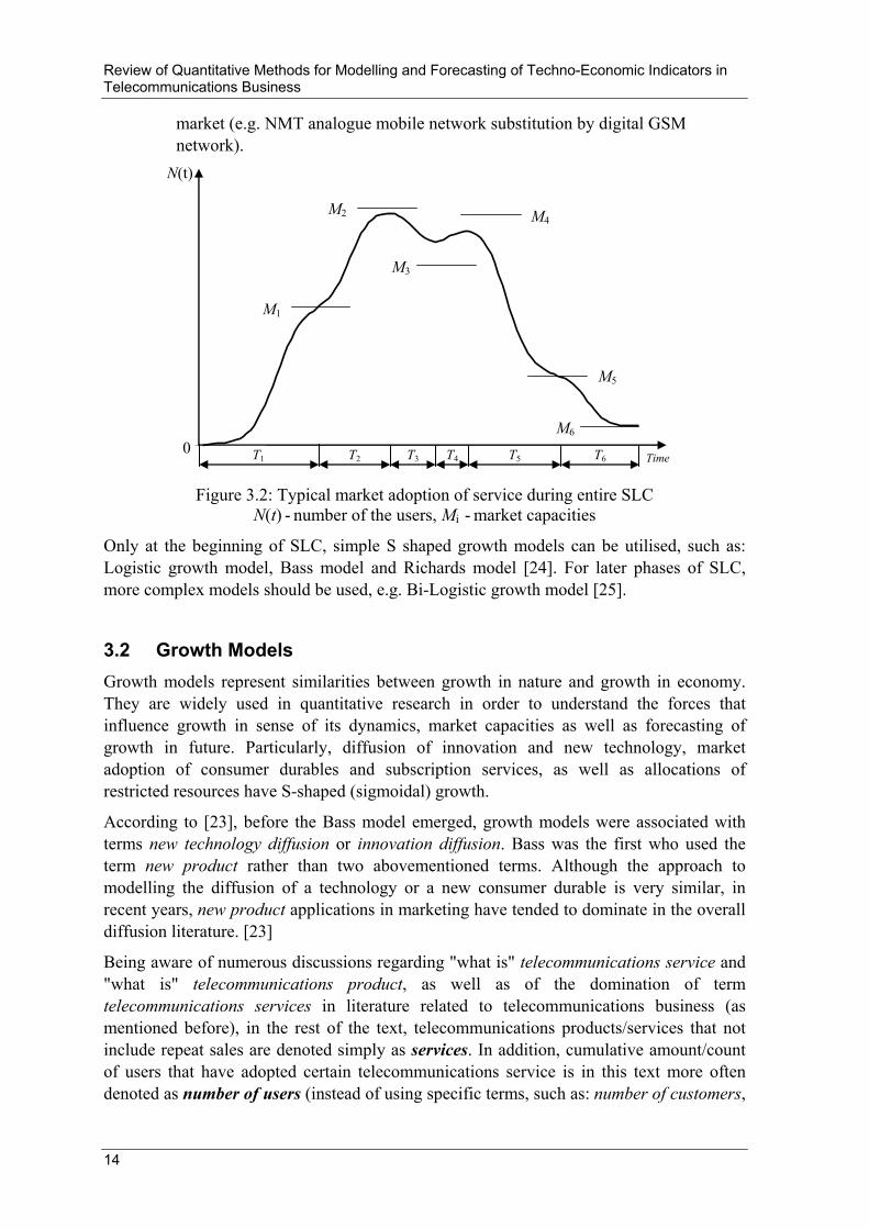
Therefore, a typical service during its life-cycle passes through the specific phases of market adoption, which can be observed through the number of service users. Figure 3.2, presents all possible combinations of number of users' growth/decline cycles: growth-growth, growth-decline, decline-growth and decline-decline with corresponding SLC time intervals: T1-T2, T2-T3, T3-T4 and T5-T6:
T1 - Service is unique and new on the market. Its market capacity M1 is identical to the current total market capacity.
T2 - New market opportunities for that service emerge (economical or technological). Its market capacity and current total market capacity are increased to M2 (e.g. introduction of pre-paid for telecom services).
T3 - Service is confronted with the first competition in unchanged market capacity (e.g. appearance of the 2nd mobile operator). Number of users N(t) decreases and service market capacity declines to M3 level.
T4 - Counter-attack of observed service provider occurs – certain number of users are coming back and/or new users are captured (e.g. in case of service price/tariff reduction). Service market capacity is increased to M4.
T5 and T6 - Further attacks from competitive service(s) lead to the number of users N(t) and market capacity M decrease. Competitive service can be identical service but offered by other provider(s), or similar, but technologically more advanced service(s). The last part of SLC is characterised with service obsolesce, substitution by new technology and service disappearance form the
Review of Quantitative Methods for Modelling and Forecasting of Techno-Economic Indicators in Telecommunications Business
14
market (e.g. NMT analogue mobile network substitution by digital GSM network).
0
N(t)
M1
M2
M3
M4
M5
M6 T1 T2 T3 T4 T5 T6 Time
Figure 3.2: Typical market adoption of service during entire SLC
N(t) - number of the users, Mi - market capacities
Only at the beginning of SLC, simple S shaped growth models can be utilised, such as: Logistic growth model, Bass model and Richards model [24]. For later phases of SLC, more complex models should be used, e.g. Bi-Logistic growth model [25].
3.2 Growth Models Growth models represent similarities between growth in nature and growth in economy. They are widely used in quantitative research in order to understand the forces that influence growth in sense of its dynamics, market capacities as well as forecasting of growth in future. Particularly, diffusion of innovation and new technology, market adoption of consumer durables and subscription services, as well as allocations of restricted resources have S-shaped (sigmoidal) growth.
According to [23], before the Bass model emerged, growth models were associated with terms new technology diffusion or innovation diffusion. Bass was the first who used the term new product rather than two abovementioned terms. Although the approach to modelling the diffusion of a technology or a new consumer durable is very similar, in recent years, new product applications in marketing have tended to dominate in the overall diffusion literature. [23]
Being aware of numerous discussions regarding "what is" telecommunications service and "what is" telecommunications product, as well as of the domination of term telecommunications services in literature related to telecommunications business (as mentioned before), in the rest of the text, telecommunications products/services that not include repeat sales are denoted simply as services. In addition, cumulative amount/count of users that have adopted certain telecommunications service is in this text more often denoted as number of users (instead of using specific terms, such as: number of customers,

Review of Quantitative Methods for Modelling and Forecasting of Techno-Economic Indicators in Telecommunications Business
15
number of subscribers, number of consumers, number of connections, number of active SIM cards, number of active lines, etc.). [24]
3.2.1 Growth Indicators
Change in number of users during time interval (t-Δt, t) consists of new adopters and the outflow:
- Leavers, which stop to use service; and - Switchers, which continue to use service, but from another provider.
Number of users at time t is: )()()()()()( tNetAddttNtOutflowtGrossAddttNtN Δ+Δ−=Δ−Δ+Δ−= (3.1)
Indicators which are commonly used related to growth are: - Growth rate (GR) - Compound annual growth rate (CAGR) and - Churn rate (CR).
Growth rate
Growth rate (GR) is a basic indicator of growth which gives percent increase (decrease) per unit time:
%100)(
)()( ⋅Δ−
Δ−−=Δ ttNttNtNGR t (3.2)
where N(t) is the number of adopted services in time point t, and N(t-Δt) is the number of adopted services in time point t-Δt. It can be shown that growth with constant growth rate has the form of exponential function:
ττ
Δ−
Δ+⋅=1
)1()()( 1
tt
GRtNtN (3.3)
Exponential growth is unlimited and does not take into consideration the influence of market capacity to diffusion of the observed service. Thus, this model can be used only on limited time interval that correspondents to the initial growth of new service.
If growth rate is given for time period Δτ which is different than Δt, formula for GRΔt can be obtained from (3.2) and (3.3), as follows:
1)1( −+= ΔΔ
ΔΔτ
τ
t
t GRGR (3.4)
For example, if growth rate is given on the yearly basis (GRY), growth rate per quarter (GRQ) is (Note: the right side approximation is based on the Taylor series for 4 xy = ):
...384
2132
34
1)1(32
41
−+−≈−+= YYYYQ
GRGRGRGRGR

Review of Quantitative Methods for Modelling and Forecasting of Techno-Economic Indicators in Telecommunications Business
16
On the contrary, yearly growth rate based on quarterly growth rate is: 4324 4641)1( QQQQQY GRGRGRGRGRGR +++=−+=
Compound annual growth rate
Compound annual growth rate (CAGR) is commonly used to show average growth rates over a range of years. It is calculated as geometric average of annual growth rates:
%1001)()(
12
1
2 ⋅⎟⎟⎠
⎞⎜⎜⎝
⎛−= −yearyear
yearNyearN
CAGR (3.5)
According to (3.5), value for CAGR strongly depends on values for number of adopted services for year1 and year2. Due to the fact that yearly number of adopted services is regularly reported on the end-of-year basis, in the cases when service starts near the end of the starting year, N(year1) is relatively low. This has the consequence in extremely high value of calculated CAGR.
Churn rate
For the measurement of relative level of outflows in (3.1), churn rate indicator CR is used (3.6):
)()(
tNtOutflowCR t
Δ=Δ (3.6)
Special attention on churn rate is given to high competitive markets such as mobile telecommunications. It is worth mentioning that some authors and/or business intelligence sources use [ N(t) + N(t-Δt) ]/2 as denominator in (3.6) instead of N(t).
If churn rate is given for a time period Δτ which is different than Δt, approximation is as follows:
ττ ΔΔ ΔΔ≈ CRtCR t
For example, churn rate given on a quarterly basis (CRQ) is approximately three times higher than monthly churn rate (CRM).
3.2.2 Determination of Growth Model Parameters
For time series growth model f (ti ;a1,a2,...,ak) based on k parameters a1,...,ak, at least k known data points (ti; N(ti)) are needed for full parameter determination. In cases when exactly k data points are available, parameters ai are solution of system of equations (3.7):
kiaaatftN kii ,...,1,0),...,,;()( 21 ==− (3.7)

Review of Quantitative Methods for Modelling and Forecasting of Techno-Economic Indicators in Telecommunications Business
17
System (3.7) is usually nonlinear system, so iterative numerical methods needed to be performed for its solution (e.g. Newton's iterative method).
In cases when k or more data points are available, weighted least squares method can be used for parameters determination to adjust the parameters of a model so as to best fit a data set. Namely, objective is to minimise sum of squared difference between data points and model evaluated points:
[ ] 221
1),...,,;()( kii
n
ii aaatftNwS −⋅=∑
= (3.8)
where wi are weights. When weights are equal to 1 (wi = 1), the method is called Ordinary least squares method (OLS).
Minimisation of (3.8) can be done by software tools such as Excel solver. Analytically, values of parameters are resulting from solution of system of equations (3.9):
kjaS
j,...,1,0 ==
∂∂
(3.9)
By the use of least squares method, values obtained for parameters are statistically smoothed, i.e. the influence on parameter values is reduced due to particular measurement errors (such as unanticipated seasonal variation, uncertain measure, etc.).
3.2.3 Growth Forecasting
Growth forecasting relies on the basic principle: growth model will be valid in the perceivable future, and forecasting result could be obtainable by extrapolation of the observed values sequentially through time and supplementary information. In general, this principle is valid only for stable markets where internal forces remain the same (e.g. same market segment boundaries, competition, cause-and-effect among services, etc.) and without change of external influences (e.g. technology, macroeconomics, purchasing power, regulatory, etc. changes). This type of forecasting belongs to quantitative time series methods.
For the forecasting purposes, parameter determination is usually focused on the time interval near the last observed data point. Thus, weights in equation (3.8) can be set to higher value for the most recent data points, than for data points in far history. For example, geometric series for weights:
1,1 >= − qq
w ini (3.10)
leads to the following weights: 1 for (the last known point) tn , 1/q for tn-1 (the penultimate known point), 1/q2 for tn-2, etc.
In some forecasting cases, model f (ti ;a1,a2,...,ak) is modified to include the fixed value of the last data point. Therefore, model has one parameter less, because ak is obtained from the equation:
0),...,,;()( 21 =− knn aaatftN (3.11)

Review of Quantitative Methods for Modelling and Forecasting of Techno-Economic Indicators in Telecommunications Business
18
The abovementioned simplification is used only when it is certain that the last data point is obtained with negligible measurement error.
Furthermore, relationships between model parameters and explanatory marketing variables can be used for the forecasting purposes, aiming at reduction of number of unknown parameters in growth model f (ti ;a1,a2,...,ak), e.g. including information of exact time when service introduction starts, time and value of anticipated sales maximum, market capacity, service price, advertising expenditures, etc.
In general, grouping of forecast results for specific market segments (e.g. separate for residential segment, for business segment and/or for segments related to specific life-styles, etc.) yields to better forecasting accuracy than aggregate forecasting performed for the whole market.
Due to measurement errors of input data, associated uncertainties of estimated model parameters can be represented by a confidence interval. Consequently, forecasting result can be represented by a prediction interval between pessimistic and optimistic values. Range depends on a determined confidence level, which is typically 95 %. Besides that, sensitivity analysis of parameters and/or explanatory variables should be deployed to examine what effect their variations have upon the forecasting result.
3.3 Logistic Growth Model The logistic model L(t) describes growth of the number of service users observed over time in a closed market, without the impact of any other service. The model is defined with three parameters: M – market capacity, a – growth rate parameter and b – time shift parameter. To emphasise model dependence of its parameters, it is convenient to indicate the model as L(t; M, a, b) [24]:
)(1)();( btae
MtLba,M,tL −−+== (3.12)
The logistic model is widely used growth model with many useful properties for technological and market development forecasting. The model (3.12) is the solution of differential equation (3.13) consisting of exponential growth term and negative feedback term. In the beginning, growth of the logistic model is identical to exponential growth, but later negative feedback slows the gradient of growth as N(t) is approaching to market capacity limit M:
⎟⎠⎞
⎜⎝⎛ −⋅=
MtLtaL
dt t dL )(1)()(
Exponentialgrowth
Negative feedback
(3.13)

Review of Quantitative Methods for Modelling and Forecasting of Techno-Economic Indicators in Telecommunications Business
19
Fig. 3.3 shows the effects of change in parameters a, b and M on the form of S-curve:
0%
25%
50%
75%
100%
B-15
B-10 B-
5 B
B+5
B+10
B+15
a = Aa = -A
0%
25%
50%
75%
100%
B-15
B-10 B-
5 B
B+5
B+10
B+15
a = Aa = 0.5·A
0%
25%
50%
75%
100%
B-15
B-10 B-
5 B
B+5
B+10
B+15
b = Bb = B-5
0%
25%
50%
75%
100%
B-15
B-10 B-
5 B
B+5
B+10
B+15
M = MCM = 0.7·MC
Figure 3.3: Effect of logistic model parameter change on the form of S-curve Cases (from top-left to bottom-right): positive and negative growth rate parameter; 50 % decrease of growth rate parameter; decrease of time shift parameter by 5 time units (e.g.
years); and 30 % decrease of market capacity parameter
3.3.1 Logistic Model through Two Fixed Points
Modification of model (3.12) which has embedded values of two data points (ts , u·M) and (te , v·M) is shown in Figure 3.4: For this case, it is suitable to define new parameters ts, Δt, u and v, which have explanatory value instead of a and b in (3.12): time ts when service perceivable starts with penetration level u, Δt – period needed for penetration grows to the level v, e.g. characteristic duration from service start to service maturity [4].

Review of Quantitative Methods for Modelling and Forecasting of Techno-Economic Indicators in Telecommunications Business
20
ts Time
Δt
L(t)
te
M v·M
u·M
Figure 3.4: Logistic model of growth defined via parameters M, ts, Δt, u and v
Parameters a and b in (3.12) should be substituted with expressions (3.14) and (3.15), which are dependent on input parameters u, v and Δt:
⎥⎦
⎤⎢⎣
⎡⎟⎠⎞
⎜⎝⎛ −−⎟
⎠⎞
⎜⎝⎛ −
Δ= 11ln11ln1
vuta (3.14)
⎟⎠⎞
⎜⎝⎛ −−⎟
⎠⎞
⎜⎝⎛ −
⎟⎠⎞
⎜⎝⎛ −
Δ+=11ln11ln
11lns
vu
uttb (3.15)
Condition that must be satisfied for equations (3.14) and (3.15) is: 0 < u < v < 1. This modified model L(t; M, ts, Δt, u, v) needs five parameters against three needed for ordinary logistic model, but the reason lies in dependence between Δt and u and v. In the case of symmetrical u and v, i.e. u = 1-v, equations become simpler [26]:
⎟⎠⎞
⎜⎝⎛ −
Δ= 11ln2
uta (3.16)
2sttb Δ+= (3.17)
Therefore, model L(t; M, ts, Δt, u) needs four parameters against three needed for ordinary logistic model, because of dependence between Δt and u:
ttt
u
MuttMtL Δ−−
⎟⎠⎞
⎜⎝⎛ −+
=Δ /)(21 s
111),,,;( s
(3.18)
Condition that must be satisfied for equation (3.18) is: 0 < u < 1.

Review of Quantitative Methods for Modelling and Forecasting of Techno-Economic Indicators in Telecommunications Business
21
3.3.2 Local Logistic Model - Logistic Model through One Fixed Point
Modification which has embedded value of one data point (tp , N(tp)) in model (3.12) is called local logistic model LL(t) [27]:
[ ] )()()(
)())(,;(
pttapp
ppp
etNMtN
tNMtNta,M,tLL
−−⋅−+
⋅= (3.19)
The local logistic model is useful for forecasting from the last observed point t > tp. The idea is that it is better to start forecasting from a known base rather than to rely on an anticipated but un-modelled reversion to a historical trend.
3.4 Bass Model The best known model for a full description of the genesis and extensions of new service market adoption is the Bass model. In distinction from the Logistic growth model, the Bass model B(t) introduces the effect of innovators via coefficient of innovation p, in differential equation of growth (3.12) which corrected deficiency of simple logistic growth ("hardly starts to grow up" problem and that t for which L(t) = 0 does not exist). The model considers a population of M adopters who are both innovators (with a constant propensity to purchase) and imitators (whose propensity to purchase is influenced by the amount of previous purchasing). [28], [29]
Effect of imitators (Logistic growth)
( ))()(1)()( tBMpM
tBtqBdt
tdB −+⎟⎠⎞
⎜⎝⎛ −=
Effect of innovators
(3.20)
Solution of differential equation (3.20) gives Bass diffusion model (3.21) defined by four parameters: M – market capacity; p – coefficient of innovation, p > 0; q – coefficient of imitation, q ≥ 0 and ts – time when service is introduced, B(ts) = 0. To emphasise model dependence of its parameters, it is convenient to indicate the model as B(t; M, p, q, ts), t ≥ ts:
))((
))((
ss
s
1
1);(ttqp
ttqp
epqeMtq,p,M,tB
−+−
−+−
+
−= (3.21)
The Bass model has a shape of S-curve, identical to the Logistic growth model, but shifted down on y-axis. Figure 3.5 shows the effects of different values of parameters p and q on form of S-curve, with fixed values for M and ts:

Review of Quantitative Methods for Modelling and Forecasting of Techno-Economic Indicators in Telecommunications Business
22
0%
25%
50%
75%
100%
Ts-5 Ts
Ts+
5
Ts+
10
Ts+
15
Ts+
20
Ts+
25
p=0.026, q=0.236p=0.139, q=0.015
0%
25%
50%
75%
100%
Ts-5 Ts
Ts+
5
Ts+
10
Ts+
15
Ts+
20
Ts+
25
p=0.053, q=0.473p=0.279, q=0.031
0%
25%
50%
75%
100%
Ts-5 Ts
Ts+
5
Ts+
10
Ts+
15
Ts+
20
Ts+
25
p=0.004, q=0.374p=0.149, q=0.002
0%
25%
50%
75%
100%
Ts-5 Ts
Ts+
5
Ts+
10
Ts+
15
Ts+
20
Ts+
25
p=0.008, q=0.747p=0.298, q=0.003
Figure 3.5: Effects of different values of parameters p and q
Chosen values are explained under the section 4.1.6: Bass model with explanatory parameters
3.4.1 Generalisation of Bass Model
Generalisations of the Bass model incorporate marketing variables, such as pricing and advertising, expanding model usage not only for early phases of SLC, but also for the phases when service faces changes of its market capacity.
The well-known Generalised Bass model incorporates the effect of service price and the effect of advertising on the likelihood of adoption. Generalised form of the Bass model in recursive form is given by [30]:
( ) )()()()()( tZttBMM
ttBqptttBtB ⋅Δ−−⋅⎟⎠⎞
⎜⎝⎛ Δ−+⋅Δ+Δ−= (3.22)
Z(t) is multiplicative factor consisting of:
⎭⎬⎫
⎩⎨⎧
Δ−Δ−−⋅+
Δ−Δ−−⋅+=
)()()(;0max
)()()(1)(
ttAttAtA
ttPttPtPtZ βα ,
where are: α – coefficient capturing the percentage increase in diffusion speed resulting from a percentage decrease in price; P(t) – price in period t; β – coefficient capturing the percentage increase in diffusion speed resulting from a percentage increase in advertising, A(t) – advertising in period t. It is worth mentioning that helpful software tools exist for this model (e.g. GBASS Excel Add-In).

Review of Quantitative Methods for Modelling and Forecasting of Techno-Economic Indicators in Telecommunications Business
23
Another well-known extension is the Norton-Bass model that describes sales of multiple generations of services. The model deals with sales of successive generations of services in those cases where adopters continue buying the service at a constant rate and buyers of earlier generations gravitate to later generations according to the Bass model cumulative distribution. Modelling of each service generation requires determination of four parameters.[31]
3.5 Richards Model The logistic model has fixed inflexion point I (b, M/2), which is not crucial for the most forecasting purposes, but it is solved with the Richards model of growth, which is sometimes called the four-parameter logistic model [32]:
[ ]cbtaeMcba,M,tR
)(1),;(
−−+= (3.23)
with parameters: M – market capacity, a – growth rate parameter, b – time shift parameter and c – shape parameter which determines position of the inflexion point. R(t) has inflexion for t = tI:
0)(lnII =′′⇔+= tR
acbt (3.24)
Minimal value of R(tI)/M arises for c → ∞ and cannot be smaller than e-1 ≈ 0.368 (minimal vertical position of an inflexion point). For c = 1 the Richards model is identical to the logistic model and R(tI)/M = 0.5 . Maximal value is without restriction, i.e. R(tI)/M → 1 for c → 0:
11
)( I1 <⎟⎠⎞
⎜⎝⎛
+=<−
c
cc
MtRe (3.25)
3.6 Recursive Growth Models In reference [33], a full description of the genesis and extensions of new-product diffusion models is given and summarised in general form of growth model as differential equation:
[ ])()()( tNMtgdt
tdN −⋅= (3.26)
where N(t) is number of users who have adopted a new product/service, M is market capacity and g(t) is function which gives different forms of the S-shaped adoption process. Based on this representation, the original Bass model has g(t) defined as: g(t) ≡ p + q⋅N(t)/M
For small time intervals Δt expression (3.26) gives general recursive form of growth models:
[ ])()()()( tNMtgttNttN −⋅⋅Δ+=Δ+ (3.27)

Review of Quantitative Methods for Modelling and Forecasting of Techno-Economic Indicators in Telecommunications Business
24
Different choices of function g(t) that is assumed to characterise the typical adoption process for different types of services and market segments. The main disadvantage of recursive growth models is that they usually have not got a correspondent explicit form.
3.7 Bi-Logistic Growth Model In reference [25], the standard 3-parameter form of the logistic growth model is multiplied in a way to model several periods (segments of SLC) of growth. In the case of two well-defined serial logistic growth pulses, it is possible to split the time-series data set in two and model each set with a separate 3-parameter logistic function. This method is limited because it is often unclear exactly where to split the data set. Cases where one process ends entirely before the second begins appear rarely. Problems arise in assigning values from the "overlap" period to the first or second pulse. The Bi-logistic growth is proposed for time-series data modelling [25], [34]:
)()()( 21 tNtNtN +=
⎥⎦
⎤⎢⎣
⎡−
Δ−+
=)()81ln(exp1
)(
11
11
ttt
MtN ;
⎥⎦
⎤⎢⎣
⎡−
Δ−+
=)()81ln(exp1
)(
22
22
ttt
MtN (3.28)
where Δti is characteristic duration, Mi is market capacity, and ti is mid-point of logistic model (point of inflexion). Based on this model, the same authors developed software tool Loglet-Lab which is capable to decompose growth into three separate logistic curves [34].
Figure 3.6: Decomposition of complex growth on auxiliary S-shaped curves
by Loglet-Lab Software tool [35]

Developing of New Growth Models for Service Life-Cycle Segments
25
4 Developing of New Growth Models for Service Life-Cycle Segments
The principles described below are followed during developing of new growth models for service life-cycle segments for the forecasting purposes:
1. Existing models, based on quantitative time series forecasting, are modified in a way to be able to accept external variables as model parameters: explanatory marketing variables, business operations information and environmental variables. Moreover, auxiliary parameters are introduced in models to enable adjusting of model to the specific practical requirements. The result is an optimal combination of qualitative and quantitative methods.
2. Existing models are modified to be suitable for forecasting purposes. Namely, usage of one model is different if the objective is to fit historical data or if the objective is to extrapolate (forecast) values in future. Based on that requirement, the existing models are reparametrised to treat the last known data point as the fixed point in model.
3. New models are developed by generalisation and/or synergy of the existing ones which enhance their usability. New models follow principles 1 and 2, as well.
4. Weighted least squares method is preferred for model parameter determination where weights are set to the higher value for the most recent data points, than for data points in far history.
5. It is assumed that growth/decline of each segment of service life-cycle is S shaped.
The above described principles are illustrated in Figure 4.1.
Mod
el
Time series history
Judg
men
tal
fore
cast
Environ-mental
variables
Forecast
Business operations
information
Explanatory parameters
Auxiliary parameters
Mod
el
Time series history
Judg
men
tal
fore
cast
Environ-mental
variables
Forecast
Business operations
information
Explanatory parameters
Auxiliary parameters
Figure 4.1: Flowchart for developing of new growth models for the forecasting purposes
Developing of New Growth Models for Service Life-Cycle Segments
26
The above described growth model, that combines qualitative and quantitative forecasting approach, should have the following general form:
N(t) = f (t; {αi}, {βi}, {γi}) where are:
{αi} Set of model parameters - resulting from fit of time series history: ti, N(ti), i = 1,...,n;
{βi} Set of explanatory parameters - resulting from qualitative/judgmental forecasting; for example: ts – time of launch; te, N (te) – target point in the future; M – (local) market capacity of service; tps – time of peak of sales, etc.
{γi} Set of auxiliary parameters in model which allows forecasting practitioner to adapt model to her/his specific needs.
By this concept, environmental variables (obtainable from public databases, agencies & associations, market research companies, company information, investment banks, etc.) such as:
- User perspective, - Competition, - Cause-and-effect of similar services (analogy & impact), - Technology, - Macroeconomics, - Regulation;
as well as business operations information (obtainable from internal knowledge sources and management) such as:
- Time of service launch, - Capability of deployment, - Capability of sales;
can be included in the growth model.
4.1 Developing of New Growth Models for the First Segment of Service Life-Cycle
In the following sections, the logistic model, the Bass model and the Richards model are analysed in detail, and the main task is to find possibilities for environmental variables incorporation. Principles stated in the introduction of Chapter 4 were used for the existing logistic model improvement and development of new models that are based on the Bass model and the Richards model: principle of local model (which modifies model for practical forecasting purposes) and principle of model through two fixed points (which is suitable for pre-launch forecasting). New models include explanatory marketing variables and exploit in a new, more efficient way the synergy of qualitative and quantitative forecasting methods and are suitable for growth forecasting related to the first segment of telecommunications service life-cycle.
In addition, the analysis of growth models that are commonly used for the forecasting purposes will define the minimum and sufficient set of input data for market adoption forecasting in the first segment of service life-cycle. [23], [24]

Developing of New Growth Models for Service Life-Cycle Segments
27
4.1.1 Analysis of Logistic Model of Growth
From (3.13) follows the discrete recursive form of logistic growth, which is useful approximation of (3.12) for small time intervals Δt:
0)(1)()()( →Δ⇔⎟⎠⎞
⎜⎝⎛ Δ−−⋅Δ−⋅Δ⋅+Δ−= t
MttLttLtattLtL (4.1)
First derivative of L(t) is given in (4):
[ ]2)(
)(
1)()(
bta
bta
eeMa
dttdLtL
−−
−−
+⋅⋅==′ (4.2)
Contrary to S-shaped cumulative adoption L(t), adoption per period (sales) is bell-shaped curve (see Figure 4.2), and it is proportional to the first derivative L'(t) of cumulative adoption:
⎟⎠⎞
⎜⎝⎛ +′⋅−≈−=
2)()()(),( 12
121221ttLtttLtLttSales (4.3)
b Time
GR
L(t)
eaΔt-1
M
L'(t) = dL(t)/dt
M/2
aM/4
(eaΔt-1)/2
0
I
Figure 4.2: Characteristic values and points of logistic model of growth
Maximum of L'(t), as well as the time point when L(t) has inflexion, is obtained from the solution of equation L''(t) = 0, where L''(t) is the second derivative of L(t):
( ) ( )[ ]( )[ ]3
2
2
2
1
1)()(bta
btabta
e
eeM-adt
tLdtL−−
−−−−
+
−⋅⋅==′′ (4.4)
From (4.4) follows that L(t) has inflexion for t = b, which is for a > 0 the maximum of L'(t), too (see Figure 4.2):
btaaMtL =>⇔=′ ;04
)(max (4.5)
Value of logistic model at point of inflexion is (see Figure 4.2) L(b) = M/2.

Developing of New Growth Models for Service Life-Cycle Segments
28
Accordingly, maximum of sales occurs at t = b when penetration is 50 %. For t1 and t2 near b, from (4.3) follows that sales in time interval [t1 , t2] can be approximated by:
4)(),( 1221
aMttttSales ⋅−≈ (4.6)
Similarly, for t1 and t2 near b, logistic model can be approximated with straight line:
42)()( MbtaMtL +−≈
Logistic model is centro-symmetric regarding inflexion point I (b, M/2):
2);();(
2Mba,M,tbLba,M,tbLM −Δ+=Δ−− (4.7)
With substitution t = b+Δt in (4.7), follows expression which directly gives the value for L(t) at centro-symmetric time point:
);2();( ba,M,tbLMba,M,tL −−=
In addition, logistic model with negative a is line-symmetric regarding axis y = M/2 to the one with positive a (see Figure 3.3, top-left graph):
2);();(
2Mba,M,tLba,M,tLM −−=− (4.8)
Asymptotes of logistic growth for positive and negative parameter a, can be summarised in (4.9):
⎩⎨⎧
<⇔=>⇔=
−∞→ 0)(00)(
limaMtL
atLt
⎩⎨⎧
>⇔=<⇔=
+∞→ 00)(0)(
limatL
aMtLt
(4.9)
Growth rate GR for time interval Δt is according to (3.2):
11
1)(
)()()(
)(−
++=
Δ−Δ−−= −−
−Δ−−
Δ bta
btta
t ee
ttLttLtLGR (4.10)
For positive a, growth rate is always positive and maximum of growth rate is when t → -∞ (see Figure 4.2):
−∞→>⇔−= ΔΔ taeGR ta
t ;01max
When t = b, growth rate is half of its maximum value:
bteGRta
t =⇔−=Δ
Δ 21
(4.11)
The above described characteristics of logistic model of growth with its explanatory attributes can be used as helpful input for estimation or assessment of model parameters for the forecasting purposes.

Developing of New Growth Models for Service Life-Cycle Segments
29
4.1.1.1 Logistic Model through Two Points for Forecasting of New Services Adoption Prior to Launch
Logistic model through two fixed points is described in section 3.3.1. Used simplification gives a framework for the forecasting of new service adoption when little or no data are available. Table 4.1 presents resulting models for typical values of characteristic duration Δt for services, service families and basic technologies according to equation (3.18, but uniformed on the same natural logarithm base e.
Table 4.1: Framework for forecasting of new services adoption prior to launch [4]
u = 5 %, v = 95 % u = 10 %, v = 90 %
Δt = 2 years )1(9442 s1)( -tt.e
MtN −−+= )1(1972 s1
)( −−−+= tt.e
MtN
Δt = 5 years )52(1781 s1)( .tt.e
MtN −−−+= )52(8790 s1
)( .tt.eMtN −−−+
=
Δt = 10 years )5(5890 s1)( −−−+
= tt.eMtN )5(4390 s1
)( −−−+= tt.e
MtN
Δt = 15 years )57(3930 s1)( .tt.e
MtN −−−+= )57(2930 s1
)( .tt.eMtN −−−+
=
Characteristic duration Δt according to [36] can be assumed as follows: services consist of units sold that have typical life-cycle of 6 to 10 quarters; service families consist of related services that have a typical business cycle of 5 years and basic technologies consist of a set of related service families that have a typical cycle of 10 to 15 years.
4.1.1.2 Logistic Model through Three Points
The logistic model L(t; M, a, b) is fully defined with three data points, (ti, N(ti)), i = 1, 2, 3 which make possible the determination of parameters M, a and b from the system of three non-linear equations:
3,2,1;1
)( )( =+
= −− ieMtN btai i
(4.12)
In general, the above system has no exact analytical solution and iterative numerical method should be used. The Newton iterative method for finding approximations to the root of a real-valued function F regarding parameter M will be applied to the equation (4.13) derived from (4.12):
0)(1
),,;( )( =−+
= −− tNeMbaMtF bta (4.13)
Parameters a and b can be obtained directly from (4.15) and (4.16) depending on assumed value for M. According to the Newton method, next approximation for M is:

Developing of New Growth Models for Service Life-Cycle Segments
30
]1[)(),,;(),,;( )(
1bta
n
n
nnn etN
MbaMtFbaMtFMM −−
+ +⋅=
∂∂
−= (4.14)
Procedure for finding parameters a, b and M:
1. Assume the initial value for M, Mn = max{N(t1), N(t2), N(t3)}, n = 1
2. Calculate the approximation for parameters a and b using value for M = Mn
⎥⎦
⎤⎢⎣
⎡⎟⎟⎠
⎞⎜⎜⎝
⎛−−⎟⎟
⎠
⎞⎜⎜⎝
⎛−= 1
)(ln1
)(ln1
2112 tNM
tNM
-tta (4.15)
⎥⎦
⎤⎢⎣
⎡−+= 1
)(ln1
11 tN
Ma
tb (4.16)
3. Calculate next approximation for M, Mn+1 according to (4.14) ]1[)( )(
313 bta
n etNM −−+ +=
4. Repeat steps 2 and 3 using value for M = Mn+1 until satisfactory accuracy ε for M is obtained, i.e.:
ε≤−+ nn MM 1
Special case - equidistant time intervals
For equidistant ti, i.e. t2 - t1 = t3 - t2 = Δt, from system of equations (4.12), analytical expressions for M, a and b can be derived:
)()()()()()()()(2)()(
3122
322
32122
1
tNtNtNtNtNtNtNtNtNtNM
−+−= (4.17)
⎟⎟⎠
⎞⎜⎜⎝
⎛−−⋅
Δ=
)()()()(
)()(ln1
23
12
1
3tNtNtNtN
tNtN
ta (4.18)
( )( )⎥⎦
⎤⎢⎣
⎡
−−+=
)()()()()(
)()(ln1
3122
212
1
31 tNtNtN
tNtNtNtN
atb (4.19)
According to the requirement that argument of logarithm must be greater than zero, equations (4.18) and (4.19) give the following conditions that have to be satisfied:
)()()( 321 tNtNtN << , or: )()()( 321 tNtNtN >> (4.20)
and:
)()(
)()(
2
3
1
2tNtN
tNtN
> (4.21)

Developing of New Growth Models for Service Life-Cycle Segments
31
Condition (4.20) is satisfied for data points that have monotone growth or monotone decline, and condition (4.21) puts limits on growth / decline gradient. It can be shown, that condition (4.21) is satisfied for growth which has a smaller gradient than exponential growth N(t)=A·B t. In other words, data points originated from exponential growth have no embedded information about growth saturation and cannot be modelled by the logistic model because M → ∞. In such cases, the described procedure for finding model parameters diverges.
4.1.2 Uncertainty of Forecasted Service Market Capacity Obtained by Logistic Model
One of the main challenges for forecasters is determination of service market capacity. In case of quantitative methods, accuracy of forecasted market capacity is directly dependent on quality of known time-series data. Quality of input data usually decreases due to: errors in measurement, effect of unexpected/unrecognised market sub-segment growth/decline, effect marketing & sales push, uncorrected seasonal deviation, etc. In [37] uncertainties and the associated confidence levels are given as a function of the uncertainty on the input data points and the length of the historical period. This study is based on some 35,000 S-curve fits on simulated data covering a variety of conditions. Resulting uncertainties for obtained parameters in [37] are given in tables and graphs but without explicit (analytical) expressions.
Based on principles used in [37] and analytical form of the logistic model through three points (see section 4.1.1.2), uncertainty of forecasted new service market capacity will be analysed in this section. According to that, the new procedure for direct analytical determination of uncertainty intervals for forecasted service market capacity is developed, enabling assessment of logistic model sensitivity to quality of input data.
Figure 4.3 brings an example of a new telecom service, where number of users for 2002, 2005 and 2008 are known but with measurement error of ±5 %. Resulting service market capacity without error should be M = 100. Encompassing possible error of measurement, market capacity lies is the interval from ML = 76.6 (-23.3 %) to MH = 152.6 (+52.6 %).
0
25
50
75
100
125
150
2000 2002 2004 2006 2008 2010 2012 2014
L(t)YL(t)YH(t)
0
25
50
75
100
125
150
2000 2002 2004 2006 2008 2010 2012 2014
L(t)YL(t)YH(t)
Figure 4.3: Uncertainty of forecasted new service market capacity [38]
Example of case when known data points have measurement error of ±5 %

Developing of New Growth Models for Service Life-Cycle Segments
32
Suppose that 3 measures of number of users Y1, Y2 and Y3 on time points t1, t2=t1+Δt, t3=t1+2Δt, are available. It is assumed that measurements have relative deviation in comparison to the theoretical logistic model of which absolute value is lower than certain error level e. [38]
3,2,1)()1()()()1( =+≤≤− itLetYtLe iii (4.22)
3,2,1)(
)()( =−= itL
tLtYei
iii (4.23)
{ }321 ,,max eeee = (4.24)
where are: Yi - measured number of users, Li - number of users according to (theoretical) logistic model, ei - relative error.
Based on measured data Yi, it is possible to find market capacity MY based on expression (4.17):
)()()()()()()()(2)()(
3122
322
32122
1
tYtYtYtYtYtYtYtYtYtYMY −
+−= (4.25)
Resulting market capacity MY is only dependent on values for Yi:
( ))();(),( 321 tYtYtYfMY = (4.26)
The lowest M, ML is obtained in case when error in ending points is negative (e1 = e3 = -e) and in the middle point positive (e2 = e) compared to the values of the logistic model L(t):
( ))()1(),()1(),()1( 321 tLetLetLefM L −+−= (4.27)
Similarly, the highest M, MH is obtained in case when error in ending points is positive (e1 = e3 = e) and in the middle point negative (e2 = -e) compared to the values of the logistic model L(t):
( ))()1(),()1(),()1( 321 tLetLetLefM H +−+= (4.28)
HL MMM ≤≤ (4.29)
Relative errors of eH and eL:
0,0 ≤−=≥−=M
MMeM
MMe LL
HH
are functions (only) of L(t1), L(t2), L(t3) and e. according to (4.27) and (4.28). Therefore, the objective is to find estimations for eH and eL depending on L(t1), L(t2), L(t3) and error level e .
High e can cause that conditions (4.20) and (4.21) are not fulfilled during calculation of MH and ML via (4.17). In addition, the obtained ML and MH must satisfy:

Developing of New Growth Models for Service Life-Cycle Segments
33
For growth: HL MMtNtNtN <<<< )()()( 321 ;
For decline: )()()( 321 tNtNtNMM LH >>>> . (4.30)
Normalisation of measured data values will reduce one dimension in representation of results for relative errors eH and eL without reducing the generality.
Introducing pi (“penetrations”):
3,2,1,)( == iMtLp i
i (4.31)
From (4.12) follows:
⎟⎟⎠
⎞⎜⎜⎝
⎛−⋅⎟⎟
⎠
⎞⎜⎜⎝
⎛−=⎟⎟
⎠
⎞⎜⎜⎝
⎛− 1
)(1
)(1
)( 31
2
2 tLM
tLM
tLM
(4.32)
and together with (4.31), gives the expression for p2:
⎟⎟⎠
⎞⎜⎜⎝
⎛−⋅⎟⎟
⎠
⎞⎜⎜⎝
⎛−+
=
11111
1
31
2
pp
p (4.33)
Putting expression for p2 in equations for eH and eL, relative errors depend only on starting penetration p1, ending penetration p3 and error level e which is suitable for direct analytical estimation as well as contour graphs representation.
1)1()1(
)1()1()1()1(2)1)(1(131
222
23
22
2321
2221
2−
−−+−+++−−+−=−=
ppepeppeepppeeppee
MMe L
L (4.34)
1)1()1(
)1()1()1()1(2)1)(1(131
222
23
22
2321
2221
2−
+−−+−+−+−−+=−=
ppepeppeepppeeppee
MMe H
H (4.35)
Contour graph for lower bound in case of error level = 1 % is presented in Figure 4.4, and in case of error level = 5 % in Figure 4.5. Contour graph for upper bound in case of error level = 1 % is presented in Figure 4.6, and in case of error level = 5 % in Figure 4.7.
For example, in case when p1= 35 %, p3= 60 %, and error level of measured data e = 1 %, lower bound for obtained market capacity is -20 % of M.
From (4.34) follows that minimum for |eL| is in cases when p1→ 0:
1)1()1()1(
)1()1(lim3
223
2
01−
−−−+−+=
→ peepeeeL
p (4.36)
In addition, when p3 → 1, eL → -e .
From (4.35) follows that minimum for eH is in cases when p1→ 0, too:
1)1()1()1(
)1()1(lim3
223
2
01−
−+−−+−=
→ peepeeeH
p (4.37)
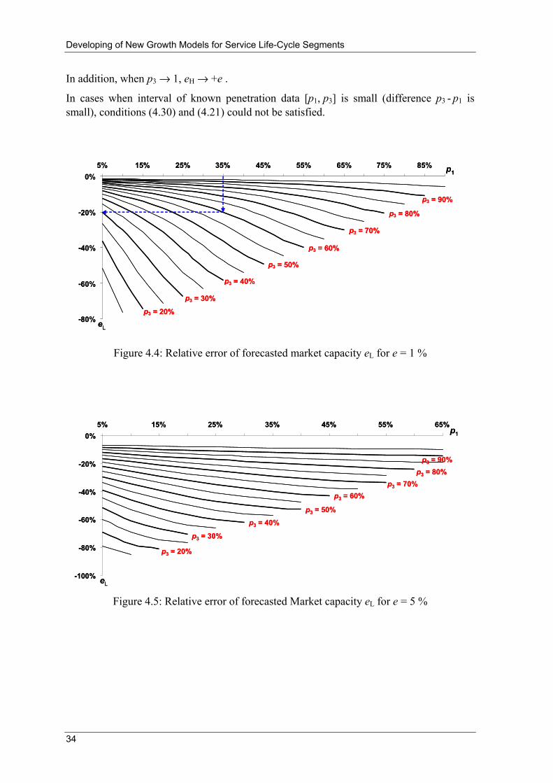
Developing of New Growth Models for Service Life-Cycle Segments
34
In addition, when p3 → 1, eH → +e .
In cases when interval of known penetration data [p1, p3] is small (difference p3 - p1 is small), conditions (4.30) and (4.21) could not be satisfied.
p 3 = 20%
p3 = 30% p3 = 40%
p3 = 50%
p3 = 60%
p3 = 70%
p3 = 80%
p 3 = 90%
- 80%
- 60%
- 40%
- 20%
0% 5% 15% 25% 35% 45% 55% 65% 75% 85%
eL
p1
p 3 = 20%
p3 = 30% p3 = 40%
p3 = 50%
p3 = 60%
p3 = 70%
p3 = 80%
p 3 = 90%
- 80%
- 60%
- 40%
- 20%
0% 5% 15% 25% 35% 45% 55% 65% 75% 85%
eL
p1
Figure 4.4: Relative error of forecasted market capacity eL for e = 1 %
p3 = 20%
p3 = 30%
p3 = 40%
p3 = 50%
p3 = 60%p3 = 70%
p3 = 80%p3 = 90%
-100%
-80%
-60%
-40%
-20%
0%5% 15% 25% 35% 45% 55% 65%
eL
p1
p3 = 20%
p3 = 30%
p3 = 40%
p3 = 50%
p3 = 60%p3 = 70%
p3 = 80%p3 = 90%
-100%
-80%
-60%
-40%
-20%
0%5% 15% 25% 35% 45% 55% 65%
eL
p1
Figure 4.5: Relative error of forecasted Market capacity eL for e = 5 %
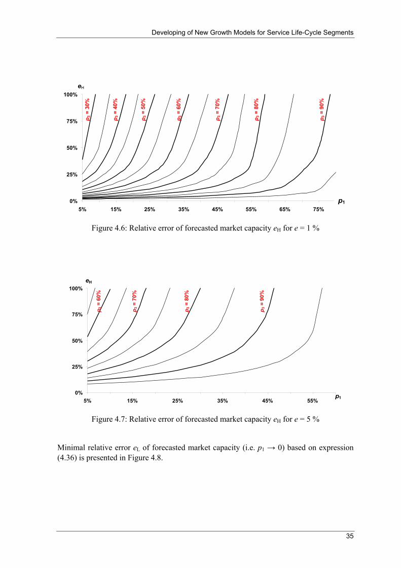
Developing of New Growth Models for Service Life-Cycle Segments
35
p 3 =
90%
0%
25%
50%
75%
100%
5% 15% 25% 35% 45% 55% 65% 75%
p 3 =
80%
p 3 =
70%
p 3 =
60%
p 3 =
50%
p 3 =
40%
p 3 =
30%
eH
p1p1
Figure 4.6: Relative error of forecasted market capacity eH for e = 1 %
0%
25%
50%
75%
100%
5% 15% 25% 35% 45% 55%
p 3 =
90%
p 3 =
80%
p 3 =
70%
p 3 =
60%
p1
eH
Figure 4.7: Relative error of forecasted market capacity eH for e = 5 %
Minimal relative error eL of forecasted market capacity (i.e. p1 → 0) based on expression (4.36) is presented in Figure 4.8.

Developing of New Growth Models for Service Life-Cycle Segments
36
-50%-45%-40%-35%-30%-25%-20%-15%-10%
-5%0%
10%
20%
30%
40%
50%
60%
70%
80%
90%
100%
e = 1%e = 2%e = 5%
-50%-45%-40%-35%-30%-25%-20%-15%-10%
-5%0%
10%
20%
30%
40%
50%
60%
70%
80%
90%
e = 1%e = 2%e = 5%
e Lp 3
-50%-45%-40%-35%-30%-25%-20%-15%-10%
-5%0%
10%
20%
30%
40%
50%
60%
70%
80%
90%
100%
e = 1%e = 2%e = 5%
-50%-45%-40%-35%-30%-25%-20%-15%-10%
-5%0%
10%
20%
30%
40%
50%
60%
70%
80%
90%
e = 1%e = 2%e = 5%
e Lp 3
Figure 4.8: Contour graph of minimal lower bound relative error eL for different error
levels e and ending penetrations p3 (i.e. p1 → 0) [38]:
Minimal relative error eH of forecasted market capacity (i.e. p1 → 0) based on expression (4.37) is presented in Figure 4.9.
0%5%
10%
15%20%25%30%35%
40%45%50%
10%
20%
30%
40%
50%
60%
70%
80%
90%
e = 1%e = 2%e = 5%
p3
0%5%
10%
15%20%25%30%35%
40%45%50%
10%
20%
30%
40%
50%
60%
70%
80%
90%
e = 1%e = 2%e = 5%
eHp
3
0%5%
10%
15%20%25%30%35%
40%45%50%
10%
20%
30%
40%
50%
60%
70%
80%
90%
e = 1%e = 2%e = 5%
p3
0%5%
10%
15%20%25%30%35%
40%45%50%
10%
20%
30%
40%
50%
60%
70%
80%
90%
e = 1%e = 2%e = 5%
eHp
3
Figure 4.9: Contour graph of minimal upper bound relative error eH for different error levels e and ending penetrations p3 (i.e. p1 → 0) [38]
Presented results have important implications; for example: if required accuracy for the market capacity is less than ±10 %, with assumed error level of input data e less than 2 %, from Figures 4.8 and 4.9 follow that the last known input data p3 should be greater than 53 %.
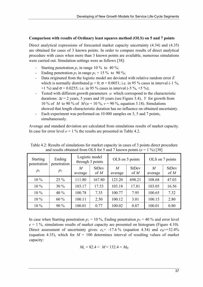
Developing of New Growth Models for Service Life-Cycle Segments
37
Comparison with results of Ordinary least squares method (OLS) on 5 and 7 points
Direct analytical expressions of forecasted market capacity uncertainty (4.34) and (4.35) are obtained for cases of 3 known points. In order to compare results of direct analytical procedure with cases when more than 3 known points are available, numerous simulations were carried out. Simulation settings were as follows [38]:
- Starting penetration p1 in range 10 % to 40 %; - Ending penetration p3 in range p1 + 15 % to 90 %; - Data originated from the logistic model are deviated with relative random error E
which is normally distributed μ = 0; σ = 0.0051; i.e. in 95 % cases in interval (-1 %, +1 %) and σ = 0.0255; i.e. in 95 % cases in interval (-5 %, +5 %);
- Tested with different growth parameters a which correspond to the characteristic durations: Δt = 2 years, 5 years and 10 years (see Figure 3.4), Y for growth from 10 % of M to 90 % of M (u = 10 %, v = 90 %, equation 3.18). Simulations showed that length characteristic duration has no influence on obtained uncertainty.
- Each experiment was performed on 10 000 samples on 3, 5 and 7 points, simultaneously.
Average and standard deviation are calculated from simulations results of market capacity. In case for error level e = 1 % the results are presented in Table 4.2.
Table 4.2: Results of simulations for market capacity in cases of 3 points direct procedure
and results obtained from OLS for 5 and 7 known points (e = 1 %) [38]
In case when Starting penetration p1 = 10 %, Ending penetration p3 = 40 % and error level e = 1 %, simulations results of market capacity are presented on histogram (Figure 4.10). Direct assessment of uncertainty gives: eL= -17.6 % (equation 4.34) and eH=+32.4% (equation 4.35), which for M = 100 determines interval of resulting values of market capacity:
ML = 82.4 < M < 132.4 = MH
Logistic model through 3 points OLS on 5 points OLS on 7 points Starting
penetration p1
Ending penetration
p3 M average
StDev of M
M average
StDev of M
M average
StDev of M
10 % 25 % 111.80 167.80 123.20 698.21 108.68 47.03
10 % 30 % 103.17 17.53 103.18 17.81 103.05 16.56
10 % 40 % 100.78 7.35 100.77 7.95 100.65 7.32
10 % 60 % 100.11 2.50 100.12 3.01 100.15 2.80
10 % 90 % 100.01 0.77 100.02 0.87 100.01 0.80

Developing of New Growth Models for Service Life-Cycle Segments
38
Simulations showed that:
- in case of 3 known points, in 99.84 % resulting values of market capacity lie in determined interval;
- in case of 5 known points in 99.88 % resulting values of market capacity lie in determined interval;
- in case of 7 known points in 99.83 % resulting values of market capacity lie in determined interval.
0
1000
2000
3000
4000
5000
6000
70 80 90 100 110 120 130 140 150 160
3 points5 points OLS7 points OLS
M = 100 ΔT =10 years 10 000 samples
Figure 4.10: Histogram of simulation results for 3 points direct procedure and results
obtained from OLS for 5 and 7 points; dashed area shows interval of uncertainty obtained by direct procedure
The procedure presented for direct analytical determination of interval of uncertainty for forecasted market capacity enables analytical assessment of model sensitivity to errors in measurement of input data.
Simulation results show that forecasted market capacity estimated by 3 points logistic model ‘direct procedure’ is comparable with the ones obtained from OLS for 5 and 7 points.
Practical implications can be very useful: in cases when ‘direct procedure’ (applied on starting, middle and ending point) according to equations (4.34) and (4.35) shows too high relative errors eL and eH, it is convenient to use service market capacity forecasted by: judgmental methods, market research surveys, benchmarkings or similar in optimistic - pessimistic interval.

Developing of New Growth Models for Service Life-Cycle Segments
39
4.1.3 Using Logistic Model of Growth for the Forecasting Purposes
The following seven cases from the forecasting praxis given in this section describe the use of the logistic model of growth and its modifications. In general, logistic model is commonly used for the forecasting of new service market adoption when interaction with other services can be neglected. [24]
General rules for all cases, when models are used for business forecasting purposes, are:
- Assess uncertainty of results related to error level of used time series data; use optimistic-pessimistic interval in cases of high uncertainty (see section 4.1.2)
- Model parameters that are obtained via judgmental assumptions should be examined in optimistic – pessimistic interval, too.
Possible cases for using the logistic model of growth for the forecasting purposes are presented in sections: 4.1.3.1 - 4.1.3.7.
Cases are examined on number of broadband fixed connections in Croatia in the period from 2003 to 2012. Data for period 2003 - 2008 have been provided from the Croatian national regulatory agency [39].
4.1.3.1 Case 1 - Extensive Set of Input Data
Known: n points, n ≥ 5 (ti, N(ti)), i = 1, 2,..., n; ∃ tj, tj > b (among them exists at least one point after inflexion)
Assumed: No need for assumptions. Model equation: (3.12)
Parameter determination:
Ordinary least squares method on logistic model L(t;M,a,b) for a, b and M determination
The fit of the model is usually very strong on the whole part of service life-cycle where service is sole on the market and can be measured with correlation coefficient R. Due to the fact that extensive set of data has to be known already, this case has low usability for practical forecasting purposes. However, it could be useful for an accurate determination of market capacity and service adoption dynamics - for forecasting by analogy of a subsequent service.

Developing of New Growth Models for Service Life-Cycle Segments
40
0
200 000
400 000
600 000
800 000
2002 2004 2006 2008 2010 2012
Data pointsModel
Year
N(t)
Figure 4.11: Logistic model in case of extensive set of input data
for broadband fixed connections in Croatia
Graphically, results of modelling of broadband fixed connections in Croatia in the period from 2003 to 2012 are presented in Figure 4.11; obtained model parameters are: M = 603 803; a = 1.1081; b = 2006.38. Correlation coefficient is: 0.9979.
4.1.3.2 Case 2 - Sufficient Set of Input Data
Known: n points, n ≥ 4 (ti, N(ti)), i = 1, 2,..., n
Assumed: No need for assumptions. Model equation: (3.19)
Parameter determination:
Ordinary least squares method on local logistic model LL(t; M,a,tp,N(tp)) for M and a determination
Suitable for forecasting of new service adoption where market capacity is unknown. The fit of the model can be measured with correlation coefficient R.

Developing of New Growth Models for Service Life-Cycle Segments
41
0
200 000
400 000
600 000
800 000
2002 2004 2006 2008 2010 2012
ModelData points
Year
N(t)
Figure 4.12: Logistic model in case of sufficient set of input data
for broadband fixed connections in Croatia
Last known point (for year 2008) is used as fixed point in the model. Graphically, results of modelling of broadband fixed connections in Croatia in the period from 2003 to 2012 are presented in Figure 4.12; obtained model parameters are: M = 619 464; a = 1.0888. Correlation coefficient is: 0.9978.
4.1.3.3 Case 3 - Sufficient Set of Input Data with Assumed Market Capacity
Known: n points, n ≥ 4 (ti, N(ti)), i = 1, 2,..., n
Assumed: Market capacity M = Ma (index a stands for assumed). Ma is usually estimated by market research and/or market segmentation techniques.
Model equation: (3.12)
Parameter determination:
Focus is on the time interval near the last observed data point, so the weighted least squares method on logistic model L(Ma,a,b;t) for a and b determination can be used
Suitable for wide-ranging forecasting purposes: for new services that are similar to previous ones on the same market; for new services which are identical to existing ones on comparable markets. The fit of the model can be measured with correlation coefficient R.
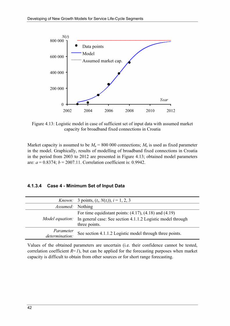
Developing of New Growth Models for Service Life-Cycle Segments
42
0
200 000
400 000
600 000
800 000
2002 2004 2006 2008 2010 2012
Data pointsModel Assumed market cap.
Year
N(t)
Figure 4.13: Logistic model in case of sufficient set of input data with assumed market
capacity for broadband fixed connections in Croatia
Market capacity is assumed to be Ma = 800 000 connections; Ma is used as fixed parameter in the model. Graphically, results of modelling of broadband fixed connections in Croatia in the period from 2003 to 2012 are presented in Figure 4.13; obtained model parameters are: a = 0.8374; b = 2007.11. Correlation coefficient is: 0.9942.
4.1.3.4 Case 4 - Minimum Set of Input Data
Known: 3 points, (ti, N(ti)), i = 1, 2, 3
Assumed: Nothing
Model equation: For time equidistant points: (4.17), (4.18) and (4.19) In general case: See section 4.1.1.2 Logistic model through three points.
Parameter determination: See section 4.1.1.2 Logistic model through three points.
Values of the obtained parameters are uncertain (i.e. their confidence cannot be tested, correlation coefficient R=1), but can be applied for the forecasting purposes when market capacity is difficult to obtain from other sources or for short range forecasting.
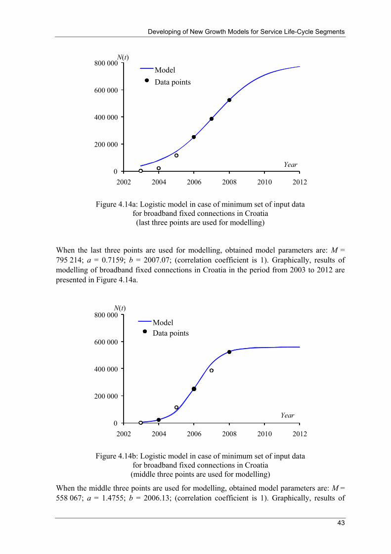
Developing of New Growth Models for Service Life-Cycle Segments
43
0
200 000
400 000
600 000
800 000
2002 2004 2006 2008 2010 2012
ModelData points
Year
N(t)
Figure 4.14a: Logistic model in case of minimum set of input data
for broadband fixed connections in Croatia (last three points are used for modelling)
When the last three points are used for modelling, obtained model parameters are: M = 795 214; a = 0.7159; b = 2007.07; (correlation coefficient is 1). Graphically, results of modelling of broadband fixed connections in Croatia in the period from 2003 to 2012 are presented in Figure 4.14a.
0
200 000
400 000
600 000
800 000
2002 2004 2006 2008 2010 2012
ModelData points
Year
N(t)
Figure 4.14b: Logistic model in case of minimum set of input data
for broadband fixed connections in Croatia (middle three points are used for modelling)
When the middle three points are used for modelling, obtained model parameters are: M = 558 067; a = 1.4755; b = 2006.13; (correlation coefficient is 1). Graphically, results of

Developing of New Growth Models for Service Life-Cycle Segments
44
modelling of broadband fixed connections in Croatia in the period from 2003 to 2012 are presented in Figure 4.14b.
4.1.3.5 Case 5 - Assumed Market Capacity and only Two Known Points
Known: 2 points, (t1 , N(t1)) and (t2 , N(t2))
Assumed: Ma market capacity Model equation: (4.15) and (4.16)
Parameter determination:
System of two non-linear equations which has an exact analytical solution for parameters a and b
Regularly used for forecasting when little data are available. Values of the obtained parameters a and b are uncertain, but the assumed market capacity M = Ma can be relatively good estimated from market research and/or market segmentation techniques which improves accuracy.
0
200 000
400 000
600 000
800 000
2002 2004 2006 2008 2010 2012
Model Data pointsAssumed market cap.
Year
N(t)
Figure 4.15a: Logistic model in case of assumed market capacity and only two known
points for broadband fixed connections in Croatia (Used points: for 2004 and for 2008)
Market capacity is assumed to be Ma = 800 000 connections; Ma is used as fixed parameter in the model. When data for 2004 and 2008 are used for modelling, obtained model parameters are: a = 1.0412; b = 2007.38. Graphically, results of modelling of broadband fixed connections in Croatia in the period from 2003 to 2012 are presented in Figure 4.15a.

Developing of New Growth Models for Service Life-Cycle Segments
45
0
200 000
400 000
600 000
800 000
2002 2004 2006 2008 2010 2012
ModelData pointsAssumed market cap.
Year
N(t)
Figure 4.15b: Logistic model in case of assumed market capacity and only two known
points for broadband fixed connections in Croatia) (Used points: for 2005 and for 2008)
Market capacity is assumed to be Ma = 800 000 connections; Ma is used as fixed parameter in the model. When data for 2005 and 2008 are used for modelling, obtained model parameters are: a = 0.8064; b = 2007.20. Graphically, results of modelling of broadband fixed connections in Croatia in the period from 2003 to 2012 are presented in Figure 4.15b.
4.1.3.6 Case 6 - Assumed Market Capacity and Characteristic Duration
Known:
ts - time when service has perceptible penetration, level of perceptible penetration u is higher than 0 (service introduction on market, start) and level of saturation v (service maturity). Values for levels u and v are conventional and usually symmetric, i.e. u = 1-v. Generally accepted values for u are 5 % or 10 % and for v 95 % or 90 %, respectively. Condition that must be satisfied is: 0 < u < v < 1.
Assumed: Ma market capacity and characteristic duration Δt. Characteristic duration is the time interval from ts to service maturity time te = ts+Δt, see Figure 3.4
Model equation: (3.18)
Parameter determination:
In general: equations (3.14) and (3.15); For symmetric u and v: equations (3.16) and (3.17) Parameters for typical characteristic durations are given in Table 4.1.
Regularly used for forecasting of new service adoption when little or no data are available. In cases of service adoption forecasting prior to service launch, a pair characteristic duration - level of saturation for service maturity is assumed by means of analogy with the existing services.
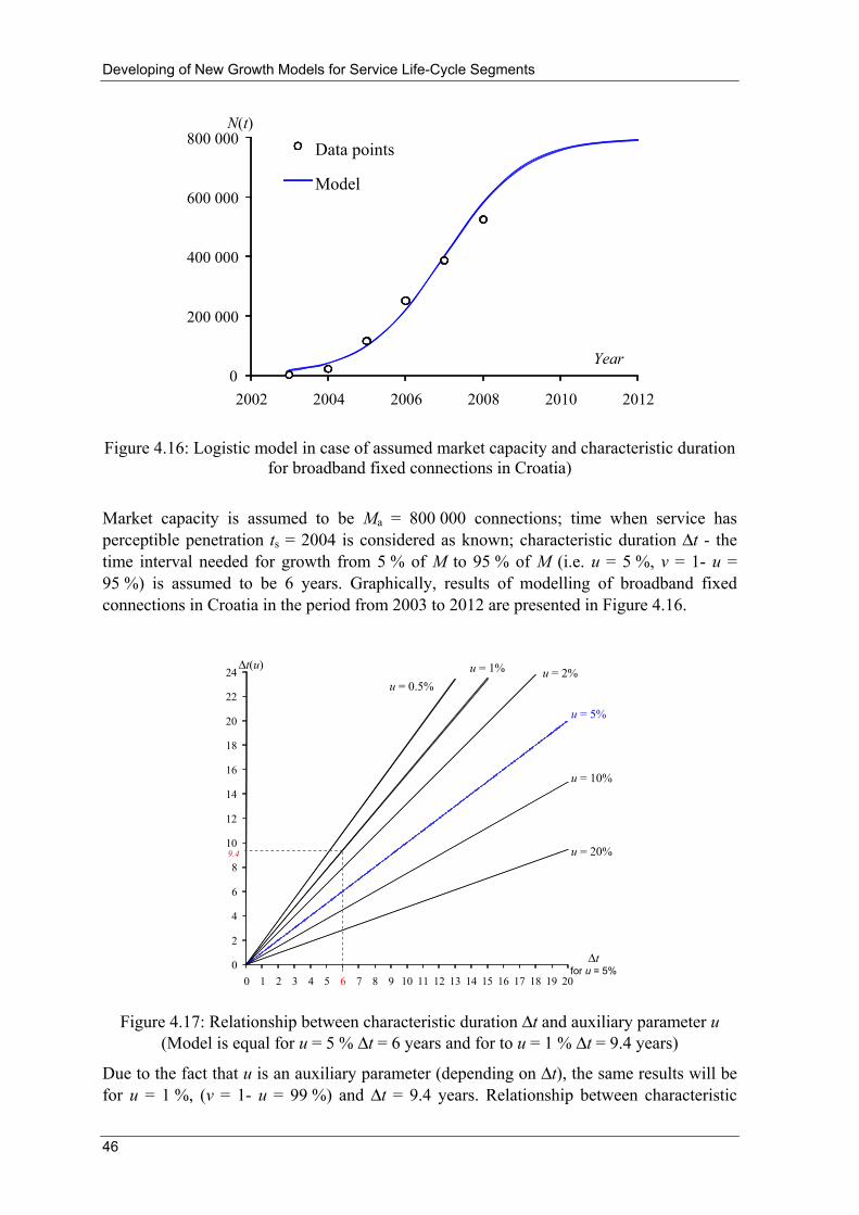
Developing of New Growth Models for Service Life-Cycle Segments
46
0
200 000
400 000
600 000
800 000
2002 2004 2006 2008 2010 2012
Data points
Model
Year
N(t)
Figure 4.16: Logistic model in case of assumed market capacity and characteristic duration
for broadband fixed connections in Croatia)
Market capacity is assumed to be Ma = 800 000 connections; time when service has perceptible penetration ts = 2004 is considered as known; characteristic duration Δt - the time interval needed for growth from 5 % of M to 95 % of M (i.e. u = 5 %, v = 1- u = 95 %) is assumed to be 6 years. Graphically, results of modelling of broadband fixed connections in Croatia in the period from 2003 to 2012 are presented in Figure 4.16.
0
2
4
6
8
10
12
14
16
18
20
22
24
0 1 2 3 4 5 6 7 8 9 10 11 12 13 14 15 16 17 18 19 20
u = 0.5%u = 1% u = 2%
u = 5%
u = 10%
u = 20%
Δt for u = 5%
9.4
Δt(u)
Figure 4.17: Relationship between characteristic duration Δt and auxiliary parameter u
(Model is equal for u = 5 % Δt = 6 years and for to u = 1 % Δt = 9.4 years)
Due to the fact that u is an auxiliary parameter (depending on Δt), the same results will be for u = 1 %, (v = 1- u = 99 %) and Δt = 9.4 years. Relationship between characteristic

Developing of New Growth Models for Service Life-Cycle Segments
47
duration Δt and auxiliary parameter u is presented in Figure 4.17, which is derived from equation 3.16. In Figure 4.17, 5 % as is taken as a baseline value for u.
4.1.3.7 Case 7 - Deployment of Explanatory Marketing Variables
Known: Various marketing variables obtained from market research surveys, market segmentation, BI tools, benchmarking, etc.
Parameter determination:
Characteristics of the logistic model of growth described in expressions: for sales (4.3), for maximum of sales (4.5) and (4.6), growth rate (4.10), growth rate at inflexion point (4.11), etc.
Explanatory marketing variables can be useful for estimation of model parameters and as test comparison with ones obtained by other means.
4.1.4 Richards Model through One Point
Based on reparameterisation for the logistic model shown in section 3.3.1, the Richards model through two fixed points (ts , u·M) and (ts + Δt , (1-u)·M); with condition that 0 < u < 1; has the form (see Figure 4.18):
( )c
tstt
c
cc
uuuMucttMtR
−
Δ
−
⎥⎥⎥⎥
⎦
⎤
⎢⎢⎢⎢
⎣
⎡
⎟⎟⎠
⎞⎜⎜⎝
⎛
−−−⋅−+⋅=Δ
−
11111111),,,,;( s (4.38)
Like the logistic model, the Richards model cannot model the time point when service is introduced, i.e. when N(t) = 0, because only for t → - ∞, R(t) approaches 0.
0%
25%
50%
75%
100%
ts ts+Δt
c = 0.2c = 10
Δt = D
0%
25%
50%
75%
100%
ts
c = 0.2c = 10
ts+Δt
Δt = D/2
Figure 4.18: Richards model for different parameters c and Δt

Developing of New Growth Models for Service Life-Cycle Segments
48
The Richards model through one fixed point (tp , N(tp)) has the following form:
c
ttac
p
pp
petN
M
MtNtcaMtLR
⎥⎥⎦
⎤
⎢⎢⎣
⎡⋅⎟⎟⎠
⎞⎜⎜⎝
⎛−+
=−− )(1
)(1
))(,,,,;( (4.39)
and could be called local Richards model due to the similarity with local logistic model. The model is useful for forecasting from the last known data point t > tp.
4.1.5 Analysis of Bass Model
The Bass model has many common characteristics with the logistic growth model. Discrete recursive form of the Bass model follows from (3.20), which is useful approximation of (3.21) for small time intervals Δt:
( ) 0)()()()( →Δ⇔Δ−−⋅⎟⎠⎞
⎜⎝⎛ Δ−+⋅Δ+Δ−= tttBM
MttBqptttBtB (4.40)
First derivative of B(t) is given in (4.41):
2))((
))((2
1
)()()(
⎥⎦
⎤⎢⎣
⎡ +
+==′−+−
−+−
s
s
ttqp
ttqp
epq
ep
qpMdt
tdBtB (4.41)
Contrary to the S-shaped cumulative adoption B(t), an adoption per period (sales) is bell-shaped curve (see Figure 4.19), and it is proportional to the first derivative B'(t) of cumulative adoption:
⎟⎠⎞
⎜⎝⎛ +′⋅−≈−=
2)()()(),( 12
121221ttBtttBtBttSales (4.42)
0
M
B(t)dB(t)/dt
ts+10 ts+20ts
q ≤ p
Mp
tI
qpqM
2)( − I
s ≥ 0.5
0ts ts+10 ts+20
B(t) dB(t)/dt
tI
q > p
qqpM
4)( 2+
qpqM
2)( −
Is < 0.5
M
Figure 4.19: Characteristic values and points of the Bass model of growth

Developing of New Growth Models for Service Life-Cycle Segments
49
Maximum of B'(t), as well as the time point when B(t) has inflexion, is obtained from the solution of equation B''(t) = 0, where B''(t) is the second derivative of B(t):
3))((
))(())((3
2
2
1
1)()()(
⎥⎦
⎤⎢⎣
⎡ +
⋅⎟⎟⎠
⎞⎜⎜⎝
⎛ −+==′′
−+−
−+−−+−
s
ss
ttqp
ttqpttqp
epq
eepq
pqpM
dttBdtB (4.43)
From (4.43) follows that B(t) has inflexion for t = tI:
0)(ln1 =′′⇔⎟⎟⎠
⎞⎜⎜⎝
⎛+
+= IsI tBpq
qptt (4.44)
and maximum of B'(t) also occurs for t = tI, when it has value of:
IttqqpMtB =⇔+=′
4)()(max
2
(4.45)
Value of the Bass model at point of inflexion is (see Figure 4.19):
qpqMtB I 2
)()( −= (4.46)
In cases when q < p, inflexion point and maximum of B'(t) occur before the service starts (tI < ts), and value of the Bass model at that point is negative according to (4.46), therefore interior maximum of B'(t) occurs at t = ts. Similarly, in cases when q = p, inflexion point and maximum of B'(t) occur when the service starts (tI = ts). For q > p, sales peak occurs in conventional sense of a SLC (tI > ts). The abovementioned is summarised in (4.47):
⎪⎪
⎩
⎪⎪
⎨
⎧
=≤⇔
=>⇔+
=′
s
I
ttpqMp
ttpqqqpM
tB,
,4
)(
)(max
2
(4.47)
Accordingly, maximum of sales occurs when penetration is (q - p)/2q in cases when q > p, (at t = tI) and in cases when q ≤ p, maximum of sales occurs at t = ts when penetration is 0.
In cases when q > p, for t1 and t2 near tI, from (4.42) follows that sales in time interval [t1 , t2] can be approximated by:
pqqqpMttttSales >⇔+⋅−≈
4)()(),(
2
1221 (4.48)
And in cases when q ≤ p, for t1 and t2 near tI, sales in time interval [t1 , t2] can be approximated by:
pqMpttttSales ≤⇔⋅−≈ )(),( 1221 (4.49)

Developing of New Growth Models for Service Life-Cycle Segments
50
The Bass model is centro-symmetric regarding inflexion point I (tI, M(q - p)/2q), see Figure 4.19:
qpqMtp,qM,ttBtp,qM,ttB
qpqM sIsI 2
)(),;(),;(2
)( −−Δ+=Δ−−− (4.50)
Growth rate GR for time interval Δt (see section 3.2. Growth models) is always positive:
)()()(
ttBttBtBGR t Δ−
Δ−−=Δ
Due to the fact that the Bass model starts from ts, B(ts) = 0, the growth rate for t → ts goes to infinity.
The above described characteristics of the Bass model with its explanatory attributes can be used as helpful input for estimation or assessment of model parameters for the forecasting purposes.
4.1.6 Bass Model with Explanatory Parameters
Parameters M and ts are descriptive and can be easily linked with market conditions, but parameters p and q have no explanatory feature. Besides that, p and q are mutually dependent while they shape the Bass model S-curve (see Figure 3.5). Namely, value of characteristic duration of service is provided only indirectly through values of p and q parameters. The idea is to replace p and q with two explanatory parameters: parameter that describes vertical shape of S-curve s and Δt - time to reach certain saturation level measured from ts. Saturation level is expected penetration v at time point ts + Δt (see explanation for Δt and v in the section 3.3.1 Logistic model through two fixed points).
Shape parameter s is chosen in order to encompass relation between amplitude of positive S-curve part and amplitude of negative S-curve part. Asymptotes of the Bass model are:
MqptB
t−=
−∞→)(lim MtB
t=
+∞→)(lim
Ratio between negative asymptote and distance of these asymptotes lies in range (0,1] which is convenient to choose as the shape parameter s, and which can be measured in percents. In fact, according to the value of s, S-curve is stretched in vertical direction (on y axis) preserving the total market capacity M.
Distance between these asymptotes is M·(1 + p/q), so shape parameter s is:
0,0,/
/ ≥>+
=+
= qppq
pqpMM
qpMs (4.51)
Characteristic values of s are:
s → 0 negative asymptote → 0, imitation prevails, curve is similar to a simple logistic growth model, (q >> p > 0),
s = 0.5 sales peak occurs at time when service starts (q = p > 0)

Developing of New Growth Models for Service Life-Cycle Segments
51
s = 1 negative asymptote → -∞, innovation prevails; curve is similar to an exponential saturation growth model, (q = 0, p > 0).
From (4.51) follows: )1()(;)( sqpqsqpp −⋅+=⋅+= (4.52)
Information about saturation point level B(ts+Δt) = vM and (3.21) give (4.53) and (4.54)
⎟⎟⎠
⎞⎜⎜⎝
⎛−
+Δ
=+)1(
1ln1vs
vt
qp , ⎟⎟⎠
⎞⎜⎜⎝
⎛−
++
=Δ)1(
1ln1vs
vqp
t (4.53)
ttt
ttt
s s
s
vsvs
vsv
MttvsMtBΔ−−
Δ−−
⎟⎟⎠
⎞⎜⎜⎝
⎛−
+⋅−+
⎟⎟⎠
⎞⎜⎜⎝
⎛−
+−=Δ
)1(1)1/1(1
)1(11
),,,,;( (4.54)
Expression (4.54) is the reparameterised Bass model with explanatory parameters (instead of p and q) where: M – market capacity; ts – time when service is introduced, B(ts) = 0, ts ≤ t, Δt –characteristic duration of service, Δt > 0, s – shape parameter, 0 < s ≤ 1; and v – penetration at time point ts + Δt, 0 ≤ v < 1. Model from (4.54), B(t; M, ts, Δt, s, v), needs four parameters: M, ts Δt and s to be determined. Value of auxiliary parameter v does not need to be determined, it just allows forecasting practitioner to choose which level of penetration he/she wants to deal with (i.e. 90 %, 95 %, etc.).
Special cases of (4.54):
For v = 0, value of model B(t) is zero:
0),,0,,;( =Δ= sttvsMtB
For s → 0 Bass model degrades into simple logistic model:
),,;(
)1(11
),,,0,;( baMtLsM
vsv
s
MttvsMtBtttss
≈−
⎟⎟⎠
⎞⎜⎜⎝
⎛−
⋅+
→Δ→Δ−−
where parameters of logistic growth model a and b are:
astb
vsv
ta s
ln,)1(
ln1 −=⎟⎠
⎞⎜⎝
⎛−Δ
=
For s = 0.5 Bass model gets a form of a halved logistic model:
MbaMtLM
vv
M
vv
vv
MttvsMtBttt
ttt
ttt
s ss
s
−=−
⎟⎠⎞
⎜⎝⎛
−++
=
⎟⎠⎞
⎜⎝⎛
−++
⎟⎠⎞
⎜⎝⎛
−+−
=Δ=Δ−−
Δ−−
Δ−−
),,2;(
111
2
111
111
),,,5.0,;(

Developing of New Growth Models for Service Life-Cycle Segments
52
This curve has a shape of the logistic model with double market capacity M but vertically shifted down by M. Parameters a and b of this "halved" logistic model are:
stbvv
ta =⎟
⎠⎞
⎜⎝⎛
−+
Δ= ,
11ln1
For s = 1 Bass model degrades into an exponential saturation growth model:
⎟⎟⎠
⎞⎜⎜⎝
⎛−−=Δ= Δ
−ttt
s
s
vMttvsMtB )1(1),,,1,;(
The following table gives the explanation of chosen values for parameters p and q presented in Figure 3.5, that are selected according to shape parameter and characteristic duration:
Graph in Figure 3.5
Shape parameter
s1
Shape parameter
s2
Characteristic duration to 95 %
penetration Δt Top-left 10 % 90 % 20 years
Top-right 10 % 90 % 10 years
Bottom-left 1 % 99 % 20 years
Bottom-right 1 % 99 % 10 years
Similarly to the framework for forecasting of new services adoption prior to launch presented in section 4.1.1.1, model (4.5) can be used in cases when little or no data is available by comparison with other similar services histories:
Table 4.3 - Reparameterised Bass model framework for new services adoption prior to launch
s - shape parameter, Δt - characteristic duration (time to reach penetration level vM measured from ts), value for v is chosen for 95 % penetration (v = 95 %)
s = 20 % s = 50 % s = 80 %
Δt = 2 years )(
)(
80.94180.91
s
s
tt
tt
M −−
−−
⋅+−
)(
)(
24.6124.61
s
s
tt
tt
M −−
−−
+−
)(
)(
97.425.0197.41
s
s
tt
tt
M −−
−−
⋅−−
Δt = 5 years )(
)(
49.24149.21
s
s
tt
tt
M −−
−−
⋅+−
)(
)(
08.2108.21
s
s
tt
tt
M −−
−−
+−
)(
)(
90.125.0190.11
s
s
tt
tt
M −−
−−
⋅−−
Δt = 10 years )(
)(
58.14158.11
s
s
tt
tt
M −−
−−
⋅+−
)(
)(
44.1144.11
s
s
tt
tt
M −−
−−
+−
)(
)(
38.125.0138.11
s
s
tt
tt
M −−
−−
⋅−−
Δt = 15 years )(
)(
36.14136.11
s
s
tt
tt
M −−
−−
⋅+−
)(
)(
28.1128.11
s
s
tt
tt
M −−
−−
+−
)(
)(
24.125.0124.11
s
s
tt
tt
M −−
−−
⋅−−

Developing of New Growth Models for Service Life-Cycle Segments
53
4.1.7 Bass Model Through One Fixed Point
Similarly to the concept of the local logistic model described in section 3.3.2 Local logistic model - logistic model through one fixed point, the Bass model with explanatory parameters which has embedded value of one data point (tp , N(tp)) has the following form:
( )
( )sp
s
sp
s
tttt
p
p
tttt
p
p
pps
tNMstN
s
tNMstN
MtNtstMtLB−−−
−−−
⎟⎟⎠
⎞⎜⎜⎝
⎛
−+⋅−+
⎟⎟⎠
⎞⎜⎜⎝
⎛
−+−
=
)()(
1)1/1(1
)()(
11
))(,,,,;( (4.55)
and could be called a local Bass model. By default, the local Bass model as well as the Bass model, has embedded value of starting point (ts , 0). The local Bass model is useful for forecasting from the last known data point t > tp.
4.1.8 Using Bass Model for the Forecasting Purposes
The Bass model is widely used for the long-term forecasting of new service market adoption when interaction with other services can be neglected. Similarly to the logistic growth model, there are several different cases when and how to use the Bass model, but generally there are four cases: Extensive set of input data; Sufficient set of input data - deploying local Bass model; Sufficient set of input data - with assumed market capacity and when little or no data is available (in cases of service market adoption forecasting prior to service launch). [24]
Similarly to the logistic model, for all cases when the Bass model is used for business forecasting purposes, rules are:
- Assess uncertainty of results related to error level of used time series data; use optimistic-pessimistic interval in cases of high uncertainty;
- Model parameters that are obtained via judgmental assumptions should be examined in optimistic – pessimistic interval, too.
Cases are examined on number of prepaid mobile users in Croatia in period of duopoly on market from 1999 to 2005. Data have been provided from WirelessIntelligence on-line business intelligence database [40].
Possible cases for using the Bass model for the forecasting purposes are presented in sections: 4.1.8.1 - 4.1.8.4.

Developing of New Growth Models for Service Life-Cycle Segments
54
4.1.8.1 Case 1 - Extensive Set of Input Data
Known: n points, n ≥ 6 (ti, N(ti)), i = 1, 2,..., n; ∃ tj, tj > b (among them exists at least one point after inflexion)
Assumed: No need for assumptions. Model equation: (3.21)
Parameter determination:
Ordinary least squares method on logistic model as B(t; M, p, q, ts), for M, p, q and ts determination
Modelling of extensive set of input data is useful for an accurate determination of the Bass model parameters for a certain service - and later for forecasting by analogy of a subsequent service or for penetration forecasting of an identical service on comparable markets.
The fit of the model is usually very strong on the whole part of service life-cycle where service is sole on the market and can be measured with correlation coefficient R. Due to the fact that extensive set of data has to be known already, this case has low usability for the practical forecasting purposes. However, it could be useful for an accurate determination of market capacity and service adoption dynamics - for forecasting by analogy of a subsequent service.
0
1 000 000
2 000 000
3 000 000
1999 2000 2001 2002 2003 2004 2005
ModelData points
Year
N(t)
Figure 4.20: Bass model in case of extensive set of input data
for prepaid mobile service in Croatia
Graphically, results of modelling of number of prepaid mobile users in Croatia in the period Q1 2000 - Q1 2005 are presented in Figure 4.20; obtained model parameters are: M = 2 603 274; p = 0.3068; q = 0.1782; ts = 1998.71. Correlation coefficient is: 0.9994.

Developing of New Growth Models for Service Life-Cycle Segments
55
4.1.8.2 Case 2 - Sufficient Set of Input Data
Known: n points, n ≥ 5 (ti, N(ti)), i = 1, 2,..., n
Assumed: No need for assumptions. Model equation: (4.55)
Parameter determination:
Ordinary least squares method on the local Bass model LB(t; M,ts,s,tp,N(tp)) for M, ts and s determination
Suitable for forecasting of new service adoption where market capacity is unknown. The fit of the model can be measured with correlation coefficient R.
0
1 000 000
2 000 000
3 000 000
1999 2000 2001 2002 2003 2004 2005
ModelData points
Year
N(t)
Figure 4.21: Bass model in case of sufficient set of input data
for prepaid mobile service in Croatia
Point for year 2004 is used as fixed point in the model. Graphically, results of modelling of number of prepaid mobile users in Croatia in the period Q1 2000 - Q1 2005 are presented in Figure 4.21; obtained model parameters are: M = 2 713 840; s = 0.5770; ts = 1998.60. Correlation coefficient is: 0.9991.

Developing of New Growth Models for Service Life-Cycle Segments
56
4.1.8.3 Case 3 - Sufficient Set of Input Data with Assumed Market Capacity
Known: n points, n ≥ 4 (ti, N(ti)), i = 1, 2,..., n
Assumed: Market capacity M = Ma (index a stands for assumed). Ma is usually estimated by market research and/or market segmentation techniques.
Model equation: (4.55) Parameter
determination: Ordinary least squares method on local Bass model LB(t; M,ts,s,tp,N(tp)) for ts and s determination
Suitable for forecasting of new service adoption, where market capacity is estimated by market research and/or market segmentation techniques. The fit of the model can be measured with correlation coefficient R.
0
1 000 000
2 000 000
3 000 000
1999 2000 2001 2002 2003 2004 2005
ModelData pointsAssumed market cap.
Year
N(t)
Figure 4.22: Bass model in case of sufficient set of input data with assumed market
capacity for prepaid mobile service in Croatia
Point for year 2004 is used as fixed point in the model. Market capacity is assumed to be Ma = 2 600 000 users; Ma is used as fixed parameter in the model. Graphically, results of modelling of number of prepaid mobile users in Croatia in the period Q1 2000 - Q1 2005 are presented in Figure 4.22; obtained model parameters are: s = 0.3162; ts = 1998.30. Correlation coefficient is: 0.9987.
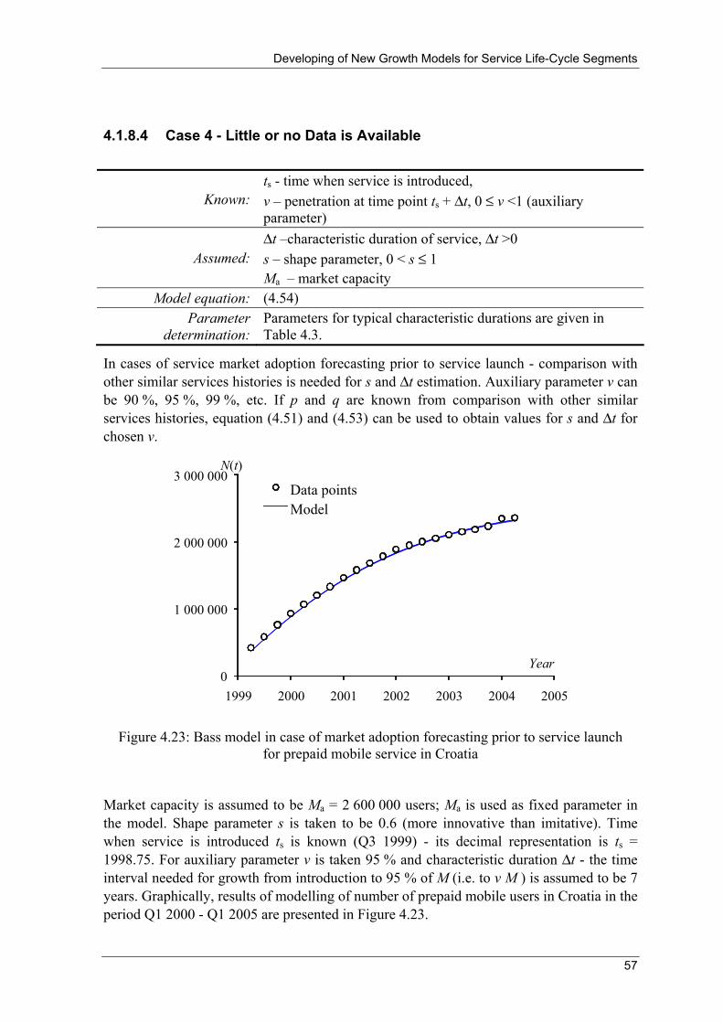
Developing of New Growth Models for Service Life-Cycle Segments
57
4.1.8.4 Case 4 - Little or no Data is Available
Known: ts - time when service is introduced, v – penetration at time point ts + Δt, 0 ≤ v <1 (auxiliary parameter)
Assumed: Δt –characteristic duration of service, Δt >0 s – shape parameter, 0 < s ≤ 1 Ma – market capacity
Model equation: (4.54) Parameter
determination: Parameters for typical characteristic durations are given in Table 4.3.
In cases of service market adoption forecasting prior to service launch - comparison with other similar services histories is needed for s and Δt estimation. Auxiliary parameter v can be 90 %, 95 %, 99 %, etc. If p and q are known from comparison with other similar services histories, equation (4.51) and (4.53) can be used to obtain values for s and Δt for chosen v.
0
1 000 000
2 000 000
3 000 000
1999 2000 2001 2002 2003 2004 2005
Data pointsModel
Year
N(t)
Figure 4.23: Bass model in case of market adoption forecasting prior to service launch
for prepaid mobile service in Croatia
Market capacity is assumed to be Ma = 2 600 000 users; Ma is used as fixed parameter in the model. Shape parameter s is taken to be 0.6 (more innovative than imitative). Time when service is introduced ts is known (Q3 1999) - its decimal representation is ts = 1998.75. For auxiliary parameter v is taken 95 % and characteristic duration Δt - the time interval needed for growth from introduction to 95 % of M (i.e. to v M ) is assumed to be 7 years. Graphically, results of modelling of number of prepaid mobile users in Croatia in the period Q1 2000 - Q1 2005 are presented in Figure 4.23.

Developing of New Growth Models for Service Life-Cycle Segments
58
4.1.9 Limitations of the Logistic, the Bass and the Richards models
Although the logistic model is widely used for the forecasting purposes, it is not suitable for modelling the service adoption when number of users grows fast instantly after the service is introduced. The reason is in the shape of logistic growth that "hardly starts to grow up". This problem is visible from conditions for equations (3.14) and (3.15), i.e. it is not possible to model the time point when service is introduced, and its penetration is 0 (i.e. u = 0), because equations will give infinity value for parameter a. This deficiency is solved with the Bass model. The second deficiency is fixed inflexion point I (b, M/2), which is not crucial for the most forecasting purposes, but it is solved with the Richards model of growth.
The Bass model is the most convenient model for market adoption forecasting of new service in sense of flexibility vs. number of free parameters that need to be estimated. Estimation of parameter values when limited data are available can be improved by introducing the Bass model with explanatory parameters. Although several generalisations of the Bass model expand model usage for later phases of PLC, numerous supplementary parameters demand a large set of known data points, which limits their application for the forecasting purposes.
Like the logistic model, the Richards model cannot model the time point when service is introduced, i.e. when N(t) = 0.
4.1.10 Generalisation of Recursive Growth Models
Differential equations for the logistic (3.13) and the Bass model (3.20):
⎟⎠⎞
⎜⎝⎛ −=
MtLtaL
dttdL )(1)()(
( ))()(1)()( tBMpM
tBtqBdt
tdB −+⎟⎠⎞
⎜⎝⎛ −=
can be rewritten in the following form:
)()()( 2 tLMataL
dttdL −= (4.56)
)()()()( 2 tBMqtBpqpM
dttdB −−+= (4.57)
Differential equations in forms (4.56) and (4.57) give idea for generalisation of growth model G(t) as differential equation:
)()()()()( 33
2210 tGbtGbtGbtGbb
dttdG n
n+++++= K (4.58)
where bi, i = 1,2,...,n are parameters of the model.

Developing of New Growth Models for Service Life-Cycle Segments
59
Illustration of relation between the generalised growth model (4.58) and other well-known growth models is given in Table 4.4. Symbol " " in table indicates usage of certain term from the generalised growth model (4.58) in specific growth model; and "-" indicates that certain term is not present in it.
Table 4.4 Relationship between generalised growth model and specific growth models
0b )(1 tGb )(22 tGb )(3
3 tGb Exponential saturation
model - -
Logistic model - - Bass model -
Richards model -
Representation in Table 4.4 helps in understanding of specific known growth model composition (for example: the Richards and the logistic model have the same deficiency because they have not got term b0 ) as well gives scheme for certain model improvement.
However, solution of differential equation of the generalised growth model becomes more complicated when it has many terms. In such cases recursive formula (4.59) for small time intervals is good approximation of (4.58) suitable for practical purposes:
[ ])()()()()( 2210 tGbtGbtGbbttGttG n
n++++Δ+=Δ+ K (4.59)
4.1.10.1 Parameter Determination of Generalised Recursive Growth Model
For parameter determination of the generalised recursive growth model in recursive form (4.59) with n+1 terms, bi, i = 0,1,...,n set of n + 2 known history points is needed. Values for bi can be determined from the system of linear equations (4.60) in matrix form:
⎥⎥⎥⎥
⎦
⎤
⎢⎢⎢⎢
⎣
⎡
Δ−
Δ−Δ−
×
⎥⎥⎥⎥
⎦
⎤
⎢⎢⎢⎢
⎣
⎡
=
⎥⎥⎥⎥
⎦
⎤
⎢⎢⎢⎢
⎣
⎡
++
−
++ tNN
tNNtNN
NN
NNNN
b
bb
nnnnn
n
n
n /)(
/)(/)(
1
11
12
23
121
11
22
1
1
0 1
M
L
MOMM
L
L
M (4.60)
where Ni are known values measured in history: N1- first point at starting time t, N2 - second point at time t+Δt, etc.
The fact that value of G(t) approaches the market capacity M in far future gives condition on bi based on (4.59):
[ ] MMbMbMbbtMtG nn
t=++++Δ+=
∞→K2
210)(lim
02210 =++++ n
n MbMbMbb K (4.61)

Developing of New Growth Models for Service Life-Cycle Segments
60
Therefore, in cases when market capacity M is known (or assumed to be known), one parameter of bi set can be determined from condition (4.61) which reduces the set of needed data points by 1.
In addition, some models (such as the logistic and the Richards model) have not got constant term b0, which additionally reduces the set of needed data points by 1 and system (4.60) becomes simpler as well:
⎥⎥⎥⎥
⎦
⎤
⎢⎢⎢⎢
⎣
⎡
Δ−
Δ−Δ−
×
⎥⎥⎥⎥
⎦
⎤
⎢⎢⎢⎢
⎣
⎡
=
⎥⎥⎥⎥
⎦
⎤
⎢⎢⎢⎢
⎣
⎡
+
−
tNN
tNNtNN
NNN
NNNNNN
b
bb
nnnnnn
n
n
n /)(
/)(/)(
1
23
121
2
2222
211
2
1 1
M
L
MOMM
L
L
M (4.62)
Summary of the described cases is given in Table 4.5.
Table 4.5 Minimum set of known data points
Presence of constant term b0
Needed data points if M is unknown
Needed data points if M is known
Exponential saturation model
(n = 1) Yes 3 2
Logistic model (n = 2) No 3 2
Bass model (n = 2) Yes 4 3 Richards model
(n = 3) No 4 3
General model (n = K) Yes K + 2 K + 1
General model (n = K) No K + 1 K
In cases when more data points are available than minimum set from Table 4.5, weighted or ordinary least squares method can be used for parameters determination to adjust the parameters of a model so as to best fit the data set, as described in section 3.2.2.
4.1.10.2 Generalised Recursive Growth Model if Market Capacity is known
Differential equation (4.63), which is based on equation (4.58), is suitable for cases when market capacity M is known (or estimated and assumed to be known):
)()()()()(1
32
32210 tG
MatG
MatG
MatGaMa
dttdG n
nn
−+++++= K (4.63)
where ai, i = 1,2,...,n are parameters of the model and M is the market capacity.

Developing of New Growth Models for Service Life-Cycle Segments
61
Namely, (4.63) simplifies condition (4.61) on model parameters, thus for G(t) approaching M, gradient (left side of (4.63)) should be 0, therefore right side of (4.63) transforms into (4.64).
nnn M
MaM
MaM
MaMaMa 1
32
322100 −+++++= K (4.64)
As a result, condition (4.61), which is inconvenient for practical use, turns into simple linear equation (4.65):
naaaa ++++= K2100 (4.65)
The generalised growth model in recursive form based on (4.63) is suitable for practical purposes in cases of small time intervals Δt:
⎥⎦⎤
⎢⎣⎡ ++++Δ+=Δ+ − )()()()()( 1
2210 tG
MatG
MatGaMattGttG n
nnK (4.66)
Parameters ai, i = 1,2,...,n of the generalised growth model (4.66) can be determined from the system of linear equations in matrix form:
⎥⎥⎥⎥
⎦
⎤
⎢⎢⎢⎢
⎣
⎡
Δ−
Δ−Δ−
×
⎥⎥⎥⎥
⎦
⎤
⎢⎢⎢⎢
⎣
⎡
−−−
−−−−−−
=
⎥⎥⎥⎥
⎦
⎤
⎢⎢⎢⎢
⎣
⎡
+
−
−
−
−
tNN
tNNtNN
MMNMMNMN
MMNMMNMNMMNMMNMN
a
aa
nnnn
nnn
nn
nn
n /)(
/)(/)(
)/()/()(
)/()/()()/()/()(
1
23
121
12
12
22
121
2
1
2
11
M
L
MOMM
L
L
M (4.67)
where Ni are known history points: N1 - first point at starting time t, N2 - second point at time t+Δt, etc. For full parameter set ai, i = 1,2,...,n determination, n+1 history points N1, N2, ..., Nn+1 are needed. Value of parameter a0 can be obtained from condition (4.65).
In cases when practical application allows that value for a0 equals 0 in model (4.66) for example as it is for the logistic and the Richards model a0 = 0), the system (4.67) becomes simpler:
⎥⎥⎥⎥
⎦
⎤
⎢⎢⎢⎢
⎣
⎡
Δ−
Δ−Δ−
×
⎥⎥⎥⎥
⎦
⎤
⎢⎢⎢⎢
⎣
⎡
−−−
−−−−−−
=
⎥⎥⎥⎥
⎦
⎤
⎢⎢⎢⎢
⎣
⎡
−
−
−−−−−
−−
−−
− tNN
tNNtNN
MMNMMNMN
MMNMMNMNMMNMMNMN
a
aa
nnnn
nnn
nn
nn
n /)(
/)(/)(
)/()/()(
)/()/()()/()/()(
1
23
121
211
211
212
22
2121
1
2
1
2
11
M
L
MOMM
L
L
M (4.68)
because only n history points N1, N2, ..., Nn are needed for full parameter set ai, i = 1,2,...,n-1 determination. The value of parameter an, can be obtained from (4.65).
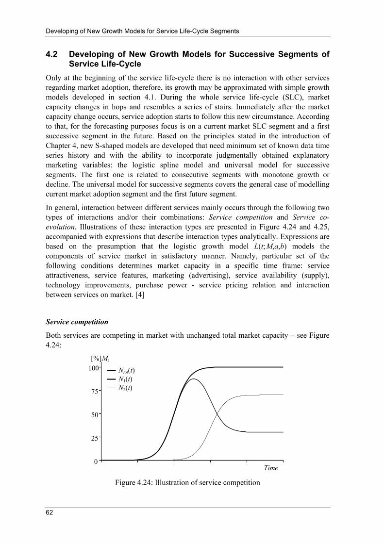
Developing of New Growth Models for Service Life-Cycle Segments
62
4.2 Developing of New Growth Models for Successive Segments of Service Life-Cycle
Only at the beginning of the service life-cycle there is no interaction with other services regarding market adoption, therefore, its growth may be approximated with simple growth models developed in section 4.1. During the whole service life-cycle (SLC), market capacity changes in hops and resembles a series of stairs. Immediately after the market capacity change occurs, service adoption starts to follow this new circumstance. According to that, for the forecasting purposes focus is on a current market SLC segment and a first successive segment in the future. Based on the principles stated in the introduction of Chapter 4, new S-shaped models are developed that need minimum set of known data time series history and with the ability to incorporate judgmentally obtained explanatory marketing variables: the logistic spline model and universal model for successive segments. The first one is related to consecutive segments with monotone growth or decline. The universal model for successive segments covers the general case of modelling current market adoption segment and the first future segment.
In general, interaction between different services mainly occurs through the following two types of interactions and/or their combinations: Service competition and Service co-evolution. Illustrations of these interaction types are presented in Figure 4.24 and 4.25, accompanied with expressions that describe interaction types analytically. Expressions are based on the presumption that the logistic growth model L(t; M,a,b) models the components of service market in satisfactory manner. Namely, particular set of the following conditions determines market capacity in a specific time frame: service attractiveness, service features, marketing (advertising), service availability (supply), technology improvements, purchase power - service pricing relation and interaction between services on market. [4]
Service competition
Both services are competing in market with unchanged total market capacity – see Figure 4.24:
0
25
50
75
100 Ntot(t)
Time
[%]Mt
N1(t) N2(t)
Figure 4.24: Illustration of service competition
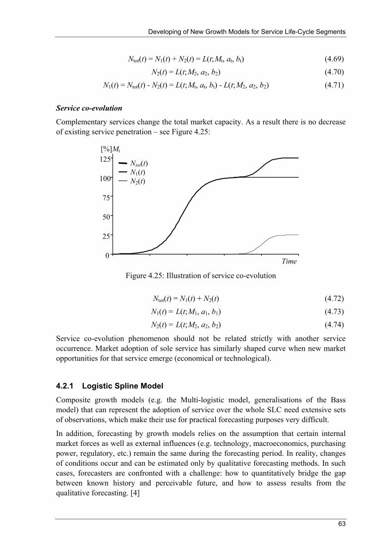
Developing of New Growth Models for Service Life-Cycle Segments
63
Ntot(t) = N1(t) + N2(t) = L(t; Mt, at, bt) (4.69)
N2(t) = L(t; M2, a2, b2) (4.70)
N1(t) = Ntot(t) - N2(t) = L(t; Mt, at, bt) - L(t; M2, a2, b2) (4.71)
Service co-evolution
Complementary services change the total market capacity. As a result there is no decrease of existing service penetration – see Figure 4.25:
0
25
50
75
100
125
Time
Ntot(t) N1(t) N2(t)
[%]Mt
Figure 4.25: Illustration of service co-evolution
Ntot(t) = N1(t) + N2(t) (4.72)
N1(t) = L(t; M1, a1, b1) (4.73)
N2(t) = L(t; M2, a2, b2) (4.74)
Service co-evolution phenomenon should not be related strictly with another service occurrence. Market adoption of sole service has similarly shaped curve when new market opportunities for that service emerge (economical or technological).
4.2.1 Logistic Spline Model
Composite growth models (e.g. the Multi-logistic model, generalisations of the Bass model) that can represent the adoption of service over the whole SLC need extensive sets of observations, which make their use for practical forecasting purposes very difficult.
In addition, forecasting by growth models relies on the assumption that certain internal market forces as well as external influences (e.g. technology, macroeconomics, purchasing power, regulatory, etc.) remain the same during the forecasting period. In reality, changes of conditions occur and can be estimated only by qualitative forecasting methods. In such cases, forecasters are confronted with a challenge: how to quantitatively bridge the gap between known history and perceivable future, and how to assess results from the qualitative forecasting. [4]

Developing of New Growth Models for Service Life-Cycle Segments
64
Analysis of typical market adoption of service during the entire SLC gives the following conclusions:
- Adoption versus time representation consists of a set of sigmoidal sub-curves. Each curve models one segment of SLC.
- Transitions between sub-curves are smooth, i.e. at least the first derivative is preserved at sub-curve junction.
By combining the principle of logistic growth (adoption curve consists of the set of S curves) plus similarity with splines gives the idea about interpolation method called logistic splines. Regularly, spline functions are used for the interpolation purposes, but originally they were strips of elastic material used to draw smooth curves through a given set of points. The most common type of interpolation spline is the cubic spline, which is formed by joining polynomials of third degree together at fixed points called knots. Cubic spline curve fitting ensures that each spline is equal to data points, the 1st derivatives are continuous at the knots, and the 2nd derivatives are continuous at the knots. The logistic splines need the minimum set of input:
- The last known data point (ts , N(ts)); - The gradient in the last known data point N'(ts); - Assumed market capacity M in the observed time interval t ∈ [ts, te]; - Assumed number of service users at the end of the observed time interval
(te , N(te)); - During the whole-observed time interval [ts, te], monotone growth (or monotone
decline) is anticipated (i.e. on the observed interval [ts, te] first derivative is either positive or negative).
The logistic spline smoothly joins the latest (known) data about the number of service users N(ts) with the assumed number of service users N(te), and locally has a form of logistic law of growth – Figure 4.26 (Growing spline) and Figure 4.27 (Declining spline). The logistic spline LS(t) is defined by four parameters: M – service market capacity, a – growth rate parameter, b – time shift parameter and c – spline parameter. To emphasise model dependence of its parameters, it is convenient to indicate the model as L(t; M, a, b):
ce
cMcbaMtLS bta ++
−= −− )(1),,,;( (4.7 )
4.2.1.1 Using Logistic Spline for the Forecasting Purposes
Unknown parameters a, b and c can be calculated from conditions:
- Starting point of the logistic spline is identical to the latest known data (4.76);
- Last point of the logistic spline is identical to the (given) assumed value N(te) (4.77);
- The logistic spline smoothly extends the existing data (4.78).
)()( ss tLStN = (4.76)
)()( ee tLStN = (4.77)
)(')(' ss tLStN = (4.78)
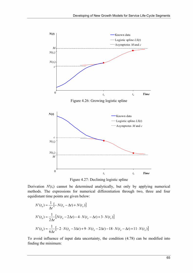
Developing of New Growth Models for Service Life-Cycle Segments
65
M
N(t)
Time
N(te)
0 ts te
N(ts) c
Known data
Logistic spline LS(t) Asymptotes M and c
Figure 4.26: Growing logistic spline
M
N(t)
Time
N(te)
0 ts te
N(ts) c
Known data Logistic spline LS(t) Asymptotes M and c
Figure 4.27: Declining logistic spline
Derivation N'(ts) cannot be determined analytically, but only by applying numerical methods. The expressions for numerical differentiation through two, three and four equidistant time points are given below:
[ ])()(1)(' s ss tNttNt
tN +Δ−−Δ
≈
[ ])(3)(4)2(21)(' s sss tNttNttN
ttN ⋅+Δ−⋅−Δ−
Δ≈
[ ])(11)(18)2(9)3(261)(' s ssss tNttNttNttN
ttN ⋅+Δ−⋅−Δ−⋅+Δ−⋅−
Δ≈
To avoid influence of input data uncertainty, the condition (4.78) can be modified into finding the minimum:

Developing of New Growth Models for Service Life-Cycle Segments
66
[ ]2ss )(')('min tLStN − (4.79)
From (4.76) and (4.77), expressions (4.81) and (4.82) for a and b can be obtained, with parameter c as a dependent variable. Parameter c cannot be achieved analytically; however, iterative minimisation of F(c) using golden section is a suitable procedure for obtaining parameter c:
[ ][ ]
2
2)(
)(
s2
sss
s
1
)()(')(')(')(⎥⎥⎥
⎦
⎤
⎢⎢⎢
⎣
⎡
+
⋅−⋅−=−=−−
−−
bta
bta
e
ecMatNtLStNcF (4.80)
Procedure is as follows: [4]
1. Choose the interval where lie possible values for c, cmin ≤ c ≤ cmax (will be discussed later, in detail)
2. Take c1 = cmin and c4 = cmax
3. Calculate two inside values for c, c2 = c4 – φ(c4 – c1) and c3 = c1 + φ(c4 – c1) according to golden section minimisation procedure, where φ is the golden section ratio (φ = 0.618...)
4. Calculate F(ci), i = 1, 2, 3, 4 using the following equations for ai and bi:
⎟⎟⎠
⎞⎜⎜⎝
⎛−−⋅
−−=
i
ii ctN
ctNtNMtNM
-tta
)()(
)()(ln1
s
e
e
s
se
(4.81)
⎟⎟⎠
⎞⎜⎜⎝
⎛−
−+=i
i ctNtNM
atb
)()(ln1
e
ee (4.82)
5. According to the calculated values for F(ci), i = 1, 2, 3, 4 decision is made about narrowing interval for c from [c1, c4] to [c1, c3] if c2 < c3 or [c2, c4] if c3 < c2. The golden section minimisation procedure is repeated from the 3rd phase to the 5th phase until resulting interval for c becomes satisfactory narrow. In practical applications, number of iterations is around 40 or less.
As stated before, there are two types of the logistic spline:
- Growing logistic spline, iff N'(ts) > 0 and N(ts) < N(te) < M (as in Figure 4.26), and
- Declining logistic spline, iff N'(ts) < 0 and N(ts) > N(te) > M, (as in Figure 4.27).
The model (4.75) can satisfy conditions (4.76) and (4.77) only if c < N(ts) for the Growing spline, and if c > N(ts) for the Declining spline. If the mentioned conditions for c are fulfilled, equations (4.81) and (4.82) have solutions. These conditions on c reflect on the determination of the interval where should lie possible values for c, cmin ≤ c ≤ cmax in the beginning of minimising F(c):
- Growing spline: initial interval is c∈(–∞, N(ts)) since c < N(ts) < N(te) < M, but in practical applications (-10·M, N(ts)) is satisfactory large initial interval for c.

Developing of New Growth Models for Service Life-Cycle Segments
67
- Declining spline: initial interval is c∈(N(ts), +∞) since M < N(te) < N(ts) < c, but in practical applications (N(ts), +10·M) is satisfactory large initial interval for c.
4.2.1.2 Limitations of Logistic Splines Usage - Assessment of Qualitative Assumptions
In ideal set of circumstances, the result of the abovementioned minimisation procedure are parameters a, b and c thus LS'(ts) = N'(ts). The logistic splines cannot satisfy the equation (4.78) if N'(ts) is too high - for the Growing spline, or too low - for the Declining spline, which will be analysed and discussed in this section.
From equation for LS'(t) it is possible to find interval where its value lies, depending on c, N(ts), N(te) and M. The first step is transforming expression for LS'(t) in form without a and b parameters:
[ ]2s )(
)(
s
s
1
)()(bta
bta
e
ecMatLS'−−
−−
+
⋅−⋅= (4.83)
From:
ce
cMtLS bta ss +
+−= −− )(1
)()( (4.84)
follows:
[ ] [ ] [ ]2
222
)( s1
)()()(btae
cMctNctLS ss −−+
−=−=− (4.85)
and:
1)(
)( s −−
−=−−
ctNcMe
s
bta (4.82)
By putting the equation (4.81) for a, expression for LS'(ts) is obtained, depending only on c, N(ts), N(te) and M, which is suitable for further analysis:
[ ] [ ]cM
tNMctNctNctN
tNMtNM
-tttLS'
i
i
−−⋅−⋅⎟⎟
⎠
⎞⎜⎜⎝
⎛−−⋅
−−= )()(
)()(
)()(ln1)( ss
s
e
e
s
ses (4.87)
In case of the Growing spline, LS'(ts) lies in range (4.88). It moves towards 0 when c approaches N(ts) and moves towards its upper limit for c → –∞.
⎟⎟⎠
⎞⎜⎜⎝
⎛−−−
<<)()(
ln)(
)(0 s
ese
ss tNM
tNM-tt
tNMtLS' (4.88)
In case of the Declining spline, LS'(ts) lies in range (4.89). It moves towards 0 when c approaches N(ts) and moves towards its lower limit for c → +∞.

Developing of New Growth Models for Service Life-Cycle Segments
68
0)()()(
ln)( s <<⎟⎟
⎠
⎞⎜⎜⎝
⎛−−−
sese
s tLS'tNMtNM
-tttNM (4.89)
Described restricted ranges for possible values of LS'(ts) have the following consequence for the forecasting purposes: depending on known values for N(ts) and N'(ts), and assumed values of M and N(te), in case of unfulfilled conditions (4.88), (4.89), the logistic spline cannot smoothly bridge the gap between known data and anticipated value in the future.
Unsmooth join of the logistic spline represents a warning to a forecaster that input assumptions are inadequate, such as:
- Predicted values for M and/or N(te) are wrong. Namely, values for M and N(te) in forecasting practice are obtained usually as the result of qualitative forecasting, which can now be assessed by logistic spline concept;
- Interval [ts, te] is consists of more than one sigmoidal curve (example in Figure 4.28).
The following Figures give examples of unsmooth join (Figure 4.28) and proper (smooth) join (Figure 4.29) of the logistic spline (Figures are screen shoots from LOST-A Excel tool).
0%
20%
40%
60%
80%
100%
1991
1992
1993
1994
1995
1996
1997
1998
1999
2000
2001
2002
2003
2004
2005
2006
2007
2008
2009
2010
2011
2012
Derivative window
Figure 4.28: Example of unsmooth join of
the logistic spline
0%
20%
40%
60%
80%
100%
1991
1992
1993
1994
1995
1996
1997
1998
1999
2000
2001
2002
2003
2004
2005
2006
2007
2008
2009
2010
2011
2012
Derivative window
Figure 4.29: Example of proper (smooth)
join of the logistic spline
The logistic spline model is suitable for forecasting of service life-cycle segments with monotone growth or decline. If this is not the case, the Universal model for successive segments of service life-cycle can be used (described in section 4.2.2). For whole service life-cycle modelling the multi-logistic growth model can be used (described in section 4.3.1).

Developing of New Growth Models for Service Life-Cycle Segments
69
4.2.1.3 Link with Bass model
The logistic spline LS(t) is identical to the Bass model B(t) (3.21) in case of the Growing spline and when parameters c < 0 and M > 0. [4]
The set of equations that establishes full link between the logistic spline LS(t; M, a, b, c) and the Bass model B(t; M, p, q, ts) is:
⇔≡ ),,,;(),,,;( stqpMtBcbaMtLS
orc
Ma
btMc
aMqMc
acp s ;ln1,, ⎟⎠⎞
⎜⎝⎛−−=
−−=
−= (4.90)
Mqpc
pq
qptbqpa −=⎟⎟
⎠
⎞⎜⎜⎝
⎛+
+=+= ,ln1, s (4.91)
The Bass model in form (3.21) requires known coefficient of innovation, p >0 and coefficient of imitation, q ≥ 0. This has the consequence that c yielded from the Bass model must be c < 0 (4.91). Although the logistic spline model is identical to the Bass model, it has no limitation on c and/or M, so spline can be unrestrictedly shifted on y-axis depending on the case.
4.2.1.4 Real Case Example for Logistic Spline Application
Application of the logistic splines is shown on the example of expired analogue mobile service in Croatia (NMT-450). The service started in 1991 very slowly because of high prices of service and mobile handsets. In the period from 1994 to 1997, it had significant growth. In 1998, service was seriously confronted with a new GSM service and went in saturation. As a counterattack, NMT operator decreased service price (cost of call per minute) on the level of approx. 15 % of GSM service price. This attempt was short-lived because GSM operators offered pre-paid system of payment and cheap mobile handsets. As a result, number of NMT users continued to decline. In Q2 2005 NMT service disappeared from the Croatian market.
Two different segments of NMT service life-cycle will be examined by the logistic splines for the forecasting purposes: growth (Figure 4.26) and decline (Figure 4.27) phase. Given information are: number of users of the NMT-450 service from the end of year (EOY) 1991 till EOY 2004.
The Growing logistic spline is used in forecast time interval from ts = 1995 to te = 1997. Values for N(ts-1Y) and N(ts) are taken as known, and values for M and N(te) are assumed. From N(1994) and N(1995), N'(1995) was obtained. Forecasting results were checked with real data in the period from 1995 to 1998. Standard statistical measure - MAPE (mean absolute percentage error) is used for this purpose (4.92).
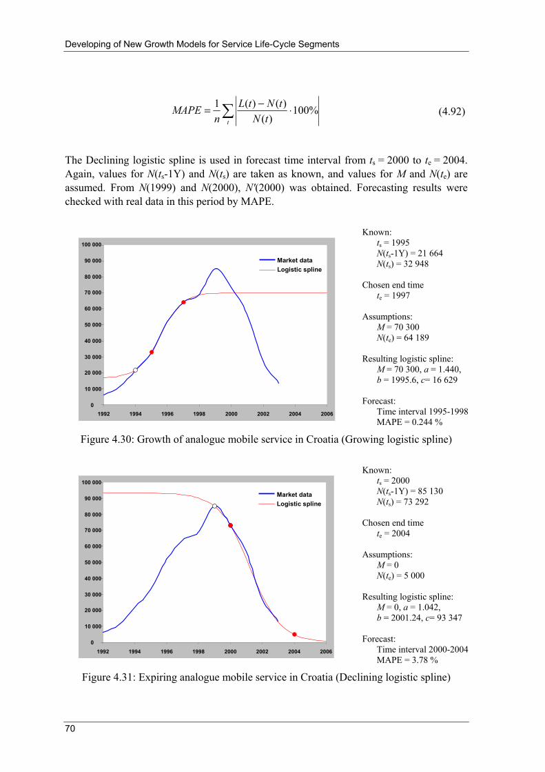
Developing of New Growth Models for Service Life-Cycle Segments
70
∑ ⋅−=t tN
tNtLn
MAPE %100)(
)()(1 (4.92)
The Declining logistic spline is used in forecast time interval from ts = 2000 to te = 2004. Again, values for N(ts-1Y) and N(ts) are taken as known, and values for M and N(te) are assumed. From N(1999) and N(2000), N'(2000) was obtained. Forecasting results were checked with real data in this period by MAPE.
1992 1994 1996 1998 2000 2002 2004 2006
Market dataLogistic spline
0 10 000 20 000 30 000 40 000 50 000 60 000 70 000 80 000 90 000
100 000
Known: ts = 1995 N(ts-1Y) = 21 664 N(ts) = 32 948
Chosen end time
te = 1997 Assumptions:
M = 70 300 N(te) = 64 189
Resulting logistic spline:
M = 70 300, a = 1.440, b = 1995.6, c= 16 629
Forecast:
Time interval 1995-1998 MAPE = 0.244 %
Figure 4.30: Growth of analogue mobile service in Croatia (Growing logistic spline)
0 10 000 20 000 30 000 40 000 50 000 60 000 70 000 80 000 90 000
100 000
1992 1994 1996 1998 2000 2002 2004 2006
Market dataLogistic spline
Known: ts = 2000 N(ts-1Y) = 85 130 N(ts) = 73 292
Chosen end time
te = 2004 Assumptions:
M = 0 N(te) = 5 000
Resulting logistic spline:
M = 0, a = 1.042, b = 2001.24, c= 93 347
Forecast:
Time interval 2000-2004 MAPE = 3.78 %
Figure 4.31: Expiring analogue mobile service in Croatia (Declining logistic spline)

Developing of New Growth Models for Service Life-Cycle Segments
71
Forecasting results are presented in Table 4.6, and values for calculated parameters are shown in Figure 4.30 and 4.31.
Table 4.6: Forecasting results for Growing logistic spline (G-LS) and Declining logistic spline (D-LS)
t [year] N(t) G-LS D-LS 1991 1 669 16 704 93 346 1992 6 320 16 940 93 342 1993 11 239 17 914 93 330 1994 21 664 21 664 93 299 1995 32 948 32 948 93 208 1996 51 857 51 428 92 954 1997 64 189 64 189 92 240 1998 68 987 68 714 90 274 1999 85 130 69 916 85 130 2000 73 292 70 208 73 292 2001 56 600 70 278 52 570 2002 27 000 70 295 29 181 2003 13 400 70 299 12 905 2004 5 000 70 300 5 000
For the abovementioned calculations, tool developed in MS Excel VBA called LOST (LOgistic Spline Trend) is used (Figure 4.32).
TrendWindow
Derivative Window
MainDialog
Pessimistic trend
Optimistic trend
Figure 4.32: Screen capture of LOST tool [35]
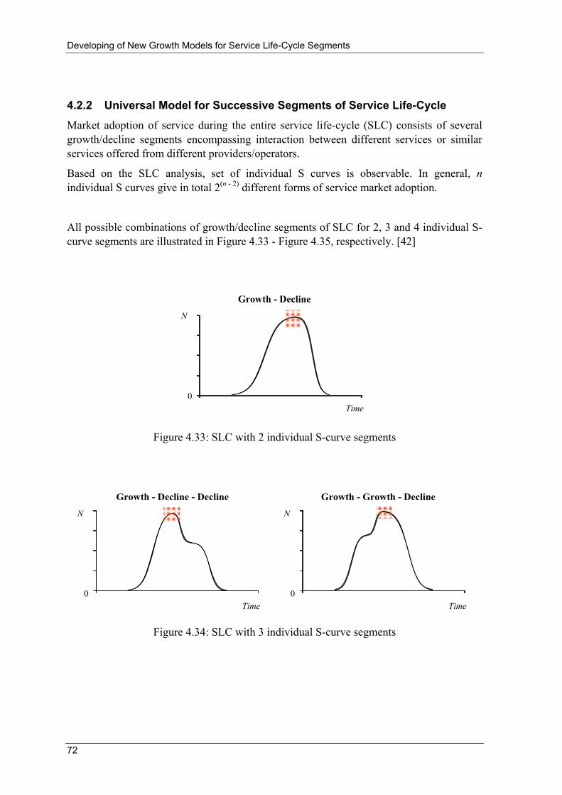
Developing of New Growth Models for Service Life-Cycle Segments
72
4.2.2 Universal Model for Successive Segments of Service Life-Cycle
Market adoption of service during the entire service life-cycle (SLC) consists of several growth/decline segments encompassing interaction between different services or similar services offered from different providers/operators.
Based on the SLC analysis, set of individual S curves is observable. In general, n individual S curves give in total 2(n - 2) different forms of service market adoption.
All possible combinations of growth/decline segments of SLC for 2, 3 and 4 individual S-curve segments are illustrated in Figure 4.33 - Figure 4.35, respectively. [42]
0
N
Time
Growth - Decline
Figure 4.33: SLC with 2 individual S-curve segments
0
N
Time
Growth - Decline - Decline
0
N
Time
Growth - Growth - Decline
Figure 4.34: SLC with 3 individual S-curve segments

Developing of New Growth Models for Service Life-Cycle Segments
73
0
N
Time
Growth - Decline - Decline - Decline
0
N
Time
Growth - Decline - Growth - Decline
0
N
Time
Growth - Growth - Decline -Decline
0
N
Time
Growth - Growth - Growth - Decline
Figure 4.35: SLC with 4 individual S-curve segments
As visible from Figure 4.33 - 4.35 (red shading areas), the logistic spline, which is designed for monotone growth-growth and decline-decline segments, cannot model connection of:
- growth - decline and - decline - growth
segments.
On the other hand, the multi-logistic model, that can model market adoption of service during the entire SLC, requires large set of known data points, which limits its application for the forecasting purposes.
However, forecaster practitioner can anticipate one consecutive part of market adoption segment in the future. On the other hand, modelling of segments that are completed in far history has no value for forecasting purposes. Therefore, the idea is to develop a model for the current market adoption segment and the first successive segment in the future.
Model based on the logistic/Bass model for this purpose has the following form: [42]
( ) Tttbta
u
MMe
MMMtf Δ−−−−
⎟⎠⎞
⎜⎝⎛ −+
−++
−+= /)(211201
0s
1111
)(
Model for the current SLC segment
Model for the first successive SLC
segment
(4.93)
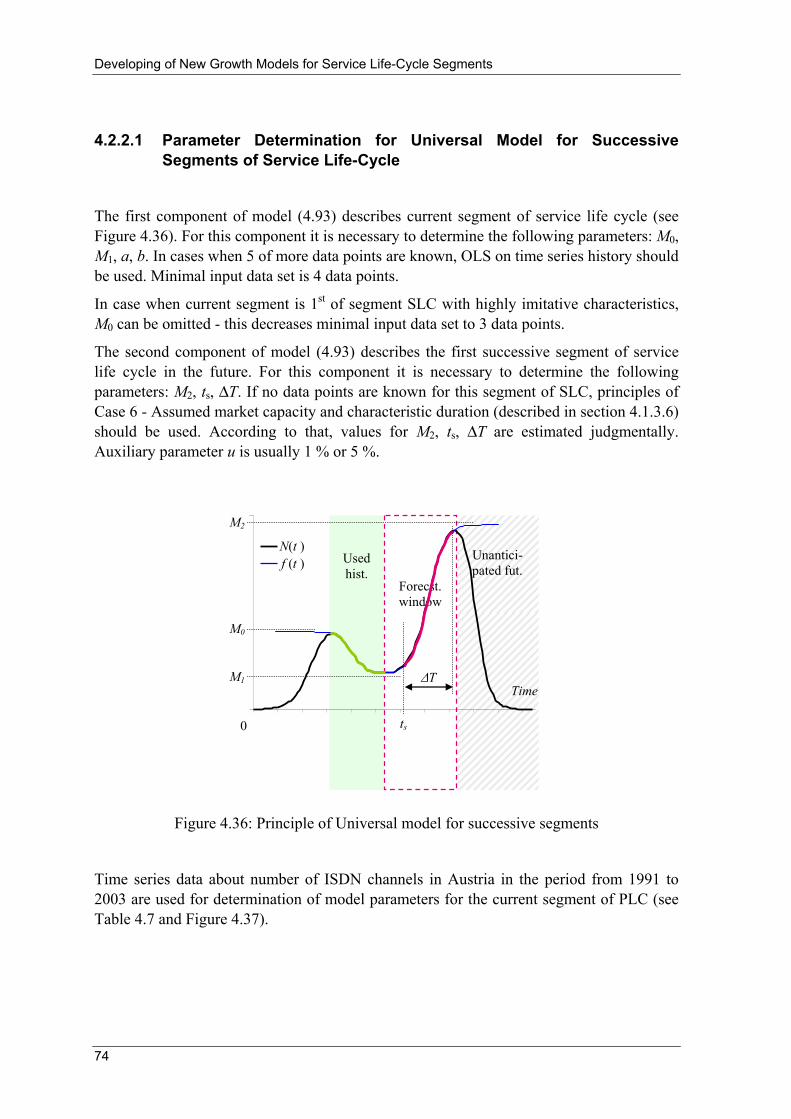
Developing of New Growth Models for Service Life-Cycle Segments
74
4.2.2.1 Parameter Determination for Universal Model for Successive Segments of Service Life-Cycle
The first component of model (4.93) describes current segment of service life cycle (see Figure 4.36). For this component it is necessary to determine the following parameters: M0, M1, a, b. In cases when 5 of more data points are known, OLS on time series history should be used. Minimal input data set is 4 data points.
In case when current segment is 1st of segment SLC with highly imitative characteristics, M0 can be omitted - this decreases minimal input data set to 3 data points.
The second component of model (4.93) describes the first successive segment of service life cycle in the future. For this component it is necessary to determine the following parameters: M2, ts, ΔT. If no data points are known for this segment of SLC, principles of Case 6 - Assumed market capacity and characteristic duration (described in section 4.1.3.6) should be used. According to that, values for M2, ts, ΔT are estimated judgmentally. Auxiliary parameter u is usually 1 % or 5 %.
Unantici-pated fut.
Used hist.
Forecst. window
0
Time
M0
M1
M2
ts
ΔT
N(t )
f (t )
Figure 4.36: Principle of Universal model for successive segments
Time series data about number of ISDN channels in Austria in the period from 1991 to 2003 are used for determination of model parameters for the current segment of PLC (see Table 4.7 and Figure 4.37).

Developing of New Growth Models for Service Life-Cycle Segments
75
0
200 000
400 000
600 000
800 000
1 000 000
1 200 000
1 400 000
1991
1992
1993
1994
1995
1996
1997
1998
1999
2000
2001
2002
2003
2004
2005
2006
2007
2008
2009
2010
2011
2012
2013
2014
2015
2016
Known data window Forecast windowData Point tp
Figure 4.37: Screen capture of tool for Universal model for successive segments
Example of ISDN service in Austria
Table 4.7: Universal model for successive segments - forecasting results Example of ISDN service in Austria [43]
Year Number of
ISDN channels Modelled number of ISDN channels
1992 0 5 314 1993 1 808 11 204 1994 10 418 24 516 1995 47 766 54 014 1996 122 560 116 601 1997 244 200 237 986 1998 427 400 437 095 1999 662 000 688 423 2000 953 720 918 321 2001 1 091 800 1 073 497 2002 1 129 000 1 155 948 2003 1 190 000 1 190 000 2004 1 213 000 1 193 769 2005 1 182 000 1 173 399 2006 1 110 000 1 125 105 2007 1 043 000 1 038 456 2008 N/A 903 078 2009 N/A 721 608 2010 N/A 520 326 2011 N/A 338 598 2012 N/A 202 519 2013 N/A 114 213 2014 N/A 62 110 2015 N/A 33 079 2016 N/A 17 417

Developing of New Growth Models for Service Life-Cycle Segments
76
Judgmentally estimated values for the first successive segment of service life cycle in the future are: M2 = 0 (ISDN service will extinct in the future), ts = 2005 (year when declining started to be perceivable), ΔT = 9 years (in 9 years service will fall to u = 5 % level).
4.3 Developing of New Growth Models for whole Service Life-Cycle Market adoption of service during the entire SLC consists of several growth/decline phases encompassing interaction between different services, and it can be modelled as the sum of discrete logistic growth models. Based on a principle of the Bi-Logistic model (3.28), and principles stated in the introduction of Chapter 4, the new multi-logistic model is developed as a composite model consisting of several logistic curves items with ability to include explanatory marketing variables.
The multi-logistic model should not be misinterpreted as a multiple logistic regression, which considers modelling of p independent variables collection, given by the equation:
)...(21 221101);...;;(
pp xaxaxaap eMxxxMLR ++++−+
=
4.3.1 Multi-Logistic Model
The multi-logistic model requires three parameters Mi, ai, and bi per item (4.94):
)(1
)2
(2
12)
1(
1
1
1...
11)(
nbt
na
nnbtabta
e
MM
e
MM
e
MtML −−−
−−−−+
−++
+
−++
= (4.94)
Market capacities increments Mi - Mi-1 represent effects of service competition in case of the negative increment (decline), or effects of service co-evolution in case of the positive increment (growth).
0
N(t)
T1 T2 T3 T4 T5 T6
Time
M1 M2 - M1
M4 - M3
M3 - M2
M5 - M4
M6 - M5
Figure 4.38: Multi-logistic model consisted of 6 logistic growth models
N(t) - number of the service users, Mi - Mi-1 market capacities (in increments)

Developing of New Growth Models for Service Life-Cycle Segments
77
Total market capacity for the observed service, according to (4.94) is:
n
n
iii
tMMMMtML =−+= ∑
=−
∞→ 211)(lim
For the illustration, adoption of service presented in Figure 3.2 is decomposed into 6 simple logistic growth models and shown in Figure 4.38.
4.3.1.1 Determination of Model Parameters
At least 3n known data points (ti; N(ti)) i = 1, 2, ..., 3n are needed for full parameter determination, where n is the number of logistic growth items in (4.94). Parameters of the multi-logistic growth model are usually obtained by the ordinary least squares method, so even more known data points are needed for satisfactory statistical smoothing of results. [44]
In praxis, modification MLM(t) of (4.94) is used, where parameters ai and bi are replaced with more descriptive ones: tSi - starting times, Δti - characteristic durations, i.e. periods needed for adoption grow from u·(Mi - Mi-1) level to (1-u)·(Mi - Mi-1) level, 0 < u < 1:
ntntt
nntttttt
u
MM
u
MM
u
MtMLM Δ−−−
Δ−−Δ−−
⎟⎠⎞
⎜⎝⎛ −+
−++
⎟⎠⎞
⎜⎝⎛ −+
−+
⎟⎠⎞
⎜⎝⎛ −+
= /)(211
2/)2(21
12
1/)1(21
1SSS
111...
111111)(
(4.95)
Generally, values accepted for u are 5 % or 10 %, so starting times tSi provide information when discrete logistic items have 5 % or 10 % penetration. Similarly, characteristic durations Δti provide information about time periods needed for discrete logistic items penetration to grow from 5 % to 95 %, or from 10 % to 90 %.
4.3.1.2 Limitations of Multi-Logistic Growth Model
The multi-logistic model is suitable for real market situations modelling on the whole SLC. However, such composite function needs determination of 3n parameters, where n is number of discrete logistic items. Therefore, a large set of known data points is needed, which limits the application of the Multi-logistic model for the forecasting purposes.
Although specific software tools exist for multi-logistic growth modelling (e.g. Loglet Lab Software), determination of model parameters can be challenging because process of minimisation of squared difference between data points and model evaluated points may diverge. In addition, resulting auxiliary curves (discrete logistic items) sometimes do not have explanatory meaning.

Developing of New Growth Models for Service Life-Cycle Segments
78
4.4 Experiences from Telecommunications Operations In this section, statistical regularities resulting from experiences from telecommunications operations will be analysed, modelled and used for forecasting purposes. Help in determination of values for specific inputs necessary for forecasting can be obtained from statistical analysis of available data. Namely, recognition of statistical laws and regularities among available data as well as possibilities of their modelling can provide forecasting inputs that were not directly accessible. Besides that, analytically modelled data are easier for further analysis and examination during business cases evaluation process.
It is important to point out that all examined S-shaped growth models are based on the assumption that there is a balance between market demand for telecommunications services and service supply from telecommunications operators. However, in cases when demand is much higher than capacity of supply, growth is not S-shaped but usually linear per segments or step-like. Therefore, proper business case must encompass not only market demand dynamics but also ability of service provisioning in general (deployment dynamics of: infrastructure / access network / aggregation network / core network / service platforms / service activation), that depends on available budget, man-power, etc.
4.4.1 Statistical Laws of New Technologies and New Services Roll-Out
Optimal roll-out for implementation of new services which require investment in network technology, mainly in access and aggregation level, can be determined from statistical data about present users of existing telecommunications services. For example, one of the inputs for ISDN roll-out which started 13 years ago, was statistics about telephone users of that time; one of input for ADSL roll-out which started 9 years ago, was statistics about heavy dial-up internet users of that time. Nowadays, similar statistics is running for FTTH rollout based on current data about xDSL and IP TV users. Introduction of two indicators for users of existing telecommunications services showed to be useful for further modelling, analysis and processing: Covering of number of users CNU and Covering of capacity of users CCU [45], [46] developed for statistics about telephone users for certain geographic area or local exchange coverage area.
Covering of number of users CNU(k)
Indicator CNU(k) is percentage of existing users which will be included in roll-out of new service if criterion is to acquire users with existing k or more telephone lines:
%if
ifkCNU m
i
m
ki 100)(
)()(
1
⋅=∑
∑
=
= (4.96)
where f(i) is amount (count) of users that exactly have i telephone line(s) - see Figure 4.39. When k = 1, all users will be acquired, so CNU(1) = 100 %.
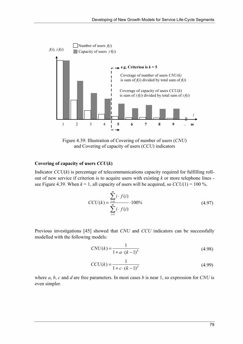
Developing of New Growth Models for Service Life-Cycle Segments
79
1 2 3 4 5 6 7 8 9 ..
Number of users f(i) f(i), i·f(i)
i
e.g. Criterion is k = 5
m
Capacity of users i·f(i)
Coverage of number of users CNU(k) is sum of f(i) divided by total sum of f(i)
Coverage of capacity of users CCU(k) is sum of i·f(i) divided by total sum of i·f(i)
Figure 4.39: Illustration of Covering of number of users (CNU)
and Covering of capacity of users (CCU) indicators
Covering of capacity of users CCU(k)
Indicator CCU(k) is percentage of telecommunications capacity required for fulfilling roll-out of new service if criterion is to acquire users with existing k or more telephone lines - see Figure 4.39. When k = 1, all capacity of users will be acquired, so CCU(1) = 100 %.
%ifi
ifikCCU m
i
m
ki 100)(
)()(
1
⋅⋅
⋅=∑
∑
=
= (4.97)
Previous investigations [45] showed that CNU and CCU indicators can be successfully modelled with the following models:
bkakCNU
)1(11)(
−⋅+= (4.98)
dkckCCU
)1(11)(
−⋅+= (4.99)
where a, b, c and d are free parameters. In most cases b is near 1, so expression for CNU is even simpler.

Developing of New Growth Models for Service Life-Cycle Segments
80
0.0001
0.001
0.01
0.1
1 1 10 100CNU(i)
CNU model
Criterion = i
CN
U(i)
Figure 4.40: Modelling Covering of number of users indicator
(example of one local exchange in Zagreb)
Modelled CNU and CCU are found to be useful for further analysis and determination of optimal criterion k in business cases for new technology and new services roll-out. Parameters of model in case which is presented in Figure 4.40 and Figure 4.41, are:
- for CNU indicator: a = 17.5918, b = 1 (Correlation coefficient = 0.9999),
- for CCU indicator: c = 1.9673, d = 0.2950 (Correlation coefficient = 0.9971).
0.01
0.1
1 10 100
CCU(i) CCU model
CC
U(i)
Criterion = i
Figure 4.41: Modelling Covering of capacity of users indicator
(example of one local exchange in Zagreb)
Relationship between Covering of number of users (CNU) and Covering of capacity (CCU) for the above described example is shown in Figure 4.42.

Developing of New Growth Models for Service Life-Cycle Segments
81
0%
25%
50%
75%
100%
0% 20% 40% 60% 80% 100% 1.4%
C NU (k )
C C U (k)
Figure 4.42: Relationship: Covering of number of users / Covering of capacity
Relationship CNU-CCU can be interpreted as: 1.4 % of all existing users on examined area utilise 25 % of all installed capacity operating on examined area, 40 % of all existing users utilise approx. 52 % of all installed capacity, etc. Marked point in Figure 4.42 (CNU = 1.4 %; CCU = 25 %) corresponds to the criterion k = 5, that means users with 5 and more existing telephone lines.
With appropriate scaling factors, relationship between existing and new service can be established in business case for new service [47]. Based on selected criterion, investment needed for roll-out is function of CNU and CCU: network access and aggregation, CPE (customer-premises equipment), in-house installation, etc. On the other hand, future revenue is only function of CCU (consumed capacity, i.e. traffic).
Models (4.98) and (4.99) were tested in several different geographical areas in Croatia with various shares of residential and business users [47]. Obtained correlation coefficients were always higher than 0.988. In fact CNU is shifted survival probability function of random variable X:
)Pr()( xXxCNU ≥=
with associated probability p(x) = Pr(X = x), probability that user has x telephone lines. Namely, probabilities p(x) found to be too scattered for modelling, but (shifted) survival function has relatively smooth shape because of its cumulative/aggregate feature, therefore it is more suitable for modelling - see Figure 4.43.

Developing of New Growth Models for Service Life-Cycle Segments
82
0.000001
0.0001
0.01
11 10 100
p(x) CNU(x)
x (existing telephone lines)
Figure 4.43: Probabilities p(x) and coverage indicator CNU(x)
in case of probability that user has x telephone lines
Upon successful modelling of coverage indicator CNU, value for probability p(x) for chosen x can be obtained from the difference of modelled coverage indicators - see (4.97):
1)(x-(x))( += CNUCNUxp (4.100)
The same principle is valid for CCU modelling. To conclude, in case of selected statistical data about existing usage of telecommunications services, modelling of coverage indicators is more successful than modelling of their probabilities (i.e. single frequencies). Based on that, probabilities and frequencies are obtainable indirectly, from a difference of modelled coverage indicators.
4.4.2 Statistical Laws of Market Segments
Statistically processed/analysed attributes of market segments, such as ranking distribution (rank-size distribution), regularly have characteristics of power laws e.g. Zipf, Pareto and Mandelbrot laws. [48]. Therefore, ranking distributions of market segments attributes can be easily modelled and their models can be used for further analysis. For better fitting results, available data should be processed in cumulative way as described in section 4.4.1. Models that are suitable for cumulative data fitting, according to the abovementioned ranking distribution regularities, will be examined in continuation.
As an example of statistical regularity of market segments attributes, distribution of business entities according to the size (number of employees) in Croatia [62] is shown in Figure 4.44.
Model for this distribution is similar to models (4.98) and (4.99):
bxaNxN
)1(1)1()(−⋅+
= (4.101)
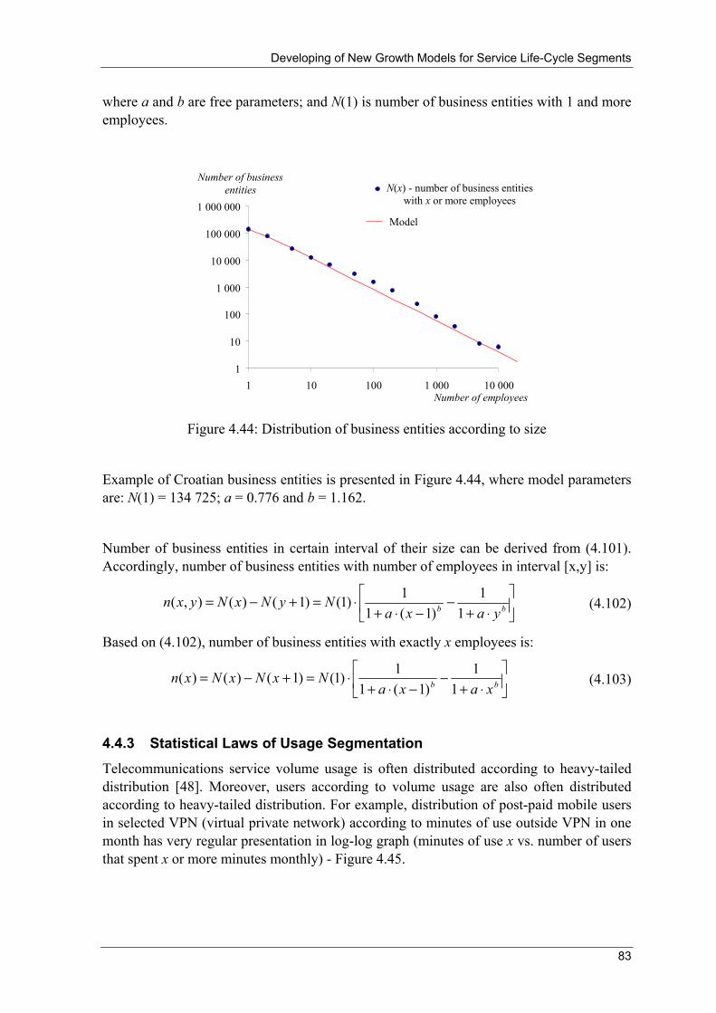
Developing of New Growth Models for Service Life-Cycle Segments
83
where a and b are free parameters; and N(1) is number of business entities with 1 and more employees.
1
10
100
1 000
10 000
100 000
1 000 000
1 10 100 1 000 10 000
N(x) - number of business entities with x or more employees
Model
Number of employees
Number of business entities
Figure 4.44: Distribution of business entities according to size
Example of Croatian business entities is presented in Figure 4.44, where model parameters are: N(1) = 134 725; a = 0.776 and b = 1.162.
Number of business entities in certain interval of their size can be derived from (4.101). Accordingly, number of business entities with number of employees in interval [x,y] is:
⎥⎦
⎤⎢⎣
⎡⋅+
−−⋅+
⋅=+−= bb yaxaNyNxNyxn
11
)1(11)1()1()(),( (4.102)
Based on (4.102), number of business entities with exactly x employees is:
⎥⎦
⎤⎢⎣
⎡⋅+
−−⋅+
⋅=+−= bb xaxaNxNxNxn
11
)1(11)1()1()()( (4.103)
4.4.3 Statistical Laws of Usage Segmentation
Telecommunications service volume usage is often distributed according to heavy-tailed distribution [48]. Moreover, users according to volume usage are also often distributed according to heavy-tailed distribution. For example, distribution of post-paid mobile users in selected VPN (virtual private network) according to minutes of use outside VPN in one month has very regular presentation in log-log graph (minutes of use x vs. number of users that spent x or more minutes monthly) - Figure 4.45.

Developing of New Growth Models for Service Life-Cycle Segments
84
1
10
100
1 000
10 000
10 100 1 000 10 000
Number of users that spentx or more minutesModel
Q
N(Q)
x [minutes]
Number of users
Figure 4.45: Distribution of users according to mobile voice minutes of use per month [49]
Model for this distribution is similar to models (4.98) and (4.99), but in this case model is extended with the auxiliary parameter Q, minimal significant traffic. In previous examples, Q was equal 1, because cases with count of certain attributes were analysed (elements of natural number set). But traffic can be measured in minutes, seconds, etc. so model should be adapted to accept such auxiliary parameter. In other words, should analysis ignore traffic less than Q volume units, than this model for number of users N(x) that spent x or more minutes, should be used:
bQxaQNQxN
)(1)();(−⋅+
= (4.104)
In the abovementioned example of post-paid VPN mobile service, Q = 50 minutes is chosen (i.e. users that spent 50 minutes or less during selected month are ignored). Value for N(Q) is 2700 users. Obtained parameters a and b are as follows: a = 7.369E-05; b = 2.195 with extremely high correlation coefficient: 0.999993. It is worth to mention that, depending on values of Q, the obtained a and b differ.
Similar ranking distribution based on the abovementioned example is presented in Figure 4.46, where users are arranged according to their monthly usage (high users first, low users last) in percentage units. For example, 20 % of all users realise 43 % of all traffic.
This relationship can be modelled by modified Hoerl model on interval 0 ≤ x ≤ 1, with fixed points f (0) = 0 and f (1) = 1:
bx xaxf ⋅= −1)( (4.105)
where x is percentage of users, f (x) is percentage of realised traffic by that users, a and b are free parameters. Values obtained for this case are: a = 0.7339; b = 0.6748 with very high correlation coefficient: 0.99992.

Developing of New Growth Models for Service Life-Cycle Segments
85
0%
25%
50%
75%
100%
0% 20% 40% 60% 80% 100%
43%
Percentage of users
Perc
enta
ge o
f usa
ge
Figure 4.46: Percentage relationship between number of users and realised traffic
(minutes of use per month)
Statistical laws and models for market segments and usage segmentation can be used for tailoring offer and price for telecommunications services as well as for examination during the business cases evaluation process.

Revenue Modelling and Forecasting
86
5 Revenue Modelling and Forecasting
5.1 Introduction to Revenue Forecasting
Revenue forecasting is the integration point of all relevant techno-economic indicators. Flow chart is presented in Figure 5.1, where are:
NTOT i (t) = Number of users in market segment i at time t; for all operators on the market (not only for the observed one)
msi (t) = Market share of chosen operator in market segment i at time t;
Volumei(t) = Standard service usage (traffic) in segment i at time t;
Price (t) = Price at time t of service volume unit.
The first step in revenue forecasting is determination of user growth dynamics per market segments. Inputs are: market capacity, time frame, saturation for whole market. Sub-steps are: identification of market segments for the observed service (e.g. business, residential, seasonal segments, etc.), estimation of total service market capacity for each segment, estimation of market penetration dynamics for each segment by analysing demand for services and external influences. Growth models described in Chapter 4 are used for this purpose.
The second step is forecasting of market share by users for the observed operator. Estimation of market share dynamics for particular operator should be done by analysing environment for the observed service for each segment. Market share models described in section 5.2 are used for this purpose.
The third step is forecasting of monthly volume (traffic) for typical user from segment i. Inputs are: user life-style, affordability, etc. Volume dynamics is strongly related to the type of service, therefore, there are no general models for volume dynamics modelling and forecasting.
The fourth step is estimation of price of service volume unit. Inputs are: costs, purchasing power, benchmarks, etc. Pricing models described in section 5.3 are used for this purpose.
Output of the fourth step is average revenue per user (ARPU) forecasted by bottom-up approach. Alternative is to include ARPU forecasted by top-down approach directly after fourth step (red arrow on flowchart - Figure 5.1). ARPU forecasting is described in section 5.4.
Revenue forecast is obtained by multiplying average number of users and ARPU for all analysed segments,.
For all the abovementioned steps, environmental variables (external influences) that should be taken into consideration are: competition, cause-and-effect of similar services (analogy & impact), technology, macroeconomics and regulatory ones.

Revenue Modelling and Forecasting
87
ΣRevenue (t)
Environment: CompetitionCause-and-effect of similar services(analogy & impact)TechnologyMacroeconomicsRegulatory
Ntot i (t) msi (t) Volumei(t)
Market segments (1..i )
Price(t)Price(t) ARPUi (t)ARPUi (t)
Top-down ARPU
Figure 5.1: Revenue forecasting flow chart [50]
5.2 Market Share Modelling and Forecasting Market share is a portion (share) of the targeted customer base (market) that a service provider actually reaches for a particular service. In general, market share can be examined not only by services / service providers but also by certain sub-services within the same service provider (e.g. prepaid vs. post paid mobile telecommunications service), by technologies (e.g. xDSL vs. FTTx in broadband access), and similar.
Appropriate modelling of market shares is prerequisite for the optimal planning of resources and investments for telecommunications operators, equipment manufactures/vendors and policy measures for the regulatory bodies. In this section, as a method for analysing the pattern of user decision-making in moving from one operator to another and consequently for market share modelling, the Markov chains are examined. Presented methods for the Markov chain transition probabilities determination enable usage of Markov chains for market share forecasting indicating what would happen if market forces remain the same over the observed time period.
New concept of the Markov chains based on diffusion growth model principles (MCDG) is developed (section 5.2.3) that provides superb modelling of diffusion of innovation and new technology, market adoption of consumer durables or subscription (telecommunications) services for the whole SLC.

Revenue Modelling and Forecasting
88
Academic research on market share models has spanned over the last twenty years. The modelling approaches have ranged from the use of predicted values of competitive behaviour [51] and when competitors' actions are forecast to simulation-based methods [52] and attraction models [53]. Other researchers use causal market share models in marketing [54], ensured that a system of equations was estimated to allow parameters to vary across segments [55]. Reference [56] applies a dynamic state-space demand system approach, while others use neural networks and genetic algorithms [57].
Reference [51] forecast market share using predicted values of competitive behaviour. Reference [56] model structure provides a convenient method of separating the short and long-run behaviour of brand market share, thereby allowing a formal analysis of their time series properties. In order to reduce high-frequency variation, the market share data are treated as time series one and smoothed by moving average techniques [58].
Discrete-time Markov process is used as a method for analysing the pattern of customer (user) decision-making in moving from one service provider to another and consequently for market share modelling [59]. Finally, [53] assesses the forecasting performance of market share models.
5.2.1 Market Share Types
For each telecom service it is possible to identify (at least) 3 different market share types: - by service provider/operator, - by (sub)service, - by technology.
Each market share type can be measured: - by units (no. of users), - by generated revenue.
Specific market share type could be modelled as a time dependent function ms(t) to understand the underlying forces and structure that produced the observed data or for the forecasting purposes. The resulting market share in the future can be used as an early warning for service providers, manufactures, vendors, etc.
5.2.2 Overall Modelling of Market Share by Markov Chains
A first-order discrete-time Markov process with finite number of states (here: number of service providers) is called Markov chain and applies if only the last purchase has an influence on the present one [59]. Therefore, the vector showing probabilities ni(t+Δt) that user is served by provider/operator i at time t+Δt is determined by:
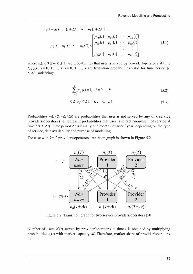
Revenue Modelling and Forecasting
89
[ ]
[ ]
( ) ( ) ( )( ) ( ) ( )
( ) ( ) ( )⎥⎥⎥⎥
⎦
⎤
⎢⎢⎢⎢
⎣
⎡
×=
=Δ+Δ+Δ+
tptptp
tptptptptptp
tntntn
ttnttnttn
kkkk
k
k
k
k
K
MOMM
L
L
L
L
10
11110
00100
10
10
)()()(
)()()(
(5.1)
where ni(t); 0 ≤ ni(t) ≤ 1; are probabilities that user is served by provider/operator i at time t; pij(t), i = 0, 1, ..., k; j = 0, 1, ..., k are transition probabilities valid for time period [t, t+Δt], satisfying:
kitpk
jij ,,0,1)(
0K==∑
= (5.2)
kjitpij ,,0,,1)(0 K=≤≤ (5.3)
Probabilities n0(t) & n0(t+Δt) are probabilities that user is not served by any of k service providers/operators (i.e. represent probabilities that user is in fact "non-user" of service at time t & t+Δt). Time period Δt is usually one month / quarter / year, depending on the type of service, data availability and purpose of modelling.
For case with k = 2 providers/operators, transition graph is shown in Figure 5.2.
t = T
t = T+Δt
p01 (T)
p00 (T)
p02 (T)
p 10(T
) p12 (T)
p 20(T)
p 21(T
)
p 22(T
)
p 11(T
)
Provider1
Provider2
Nonusers
Provider1
Provider2
Nonusers
n0(T) n1(T) n2(T)
n0(T+Δt) n1(T+Δt) n2(T+Δt)
t = T
t = T+Δt
p01 (T)
p00 (T)
p02 (T)
p 10(T
) p12 (T)
p 20(T)
p 21(T
)
p 22(T
)
p 11(T
)
Provider1
Provider2
Nonusers
Provider1
Provider2
Nonusers
n0(T) n1(T) n2(T)
n0(T+Δt) n1(T+Δt) n2(T+Δt)
Figure 5.2: Transition graph for two service providers/operators [50]
Number of users Ni(t) served by provider/operator i at time t is obtained by multiplying probabilities ni(t) with market capacity M. Therefore, market share of provider/operator i is:

Revenue Modelling and Forecasting
90
)(1)(
)(
)(
)(
)()(0
11
tntn
tnM
tnM
tN
tNtms ik
jj
ik
jj
ii −
=⋅
⋅==
∑∑==
(5.4)
In cases when transition probabilities remain the same over the observed time period, i.e., pij(t) = pij, t∈[t1, t2], Markov chain is called time-homogeneous Markov chain. This case corresponds to the one in which market forces remain the same during the observed time period [t1, t2]. Example of time-homogeneous Markov chain data for two service providers/operators is shown in Figure 5.3.
Transition matrix of time-homogeneous Markov chain P consisted of transition probabilities pij has descriptive features and can be linked with explanatory marketing variables [50]. For example, Churn and Churn rate (see section 3.2.1) of service provider/operator i at time t for period Δt is:
( ) kiptNtChurn iiii ,...,1,1)()( =−⋅=
Ordinary Markov chain model
0
0.5
1 n0 n1 n2
Time
Figure 5.3: Time-homogeneous Markov chain model for two service providers/operators; n1 and n2 are probabilities that user is served by provider/operator 1 and 2, n0 is probability
that user is still "non-user" of service
It is interesting that for time-homogeneous Markov chain the resulting Churn rate is constant (see Figure 5.4:).
( ) kiptChurnRate iii ,...,1,1)( =−=
Similarly, Gross add and Net add are:
kjkiptNtGrossAddij
jiii ,...,0;,...,1,)()( ==⋅=∑≠
kitttNetAdd iii ,...,1),(Churn)(GrossAdd)( =−=

Revenue Modelling and Forecasting
91
Ordinary Markov chain model
0
0.5
1
0%
25%
50%
75%
100% n1 ChurnRate1
Time
Figure 5.4: Churn rate for 1st service provider/operator based on time-homogeneous Markov chain model from Figure 5.3
Long-term behaviour of time-homogeneous Markov chain shows that it can have steady (equilibrium) state. For transition matrix P, vector U is called equilibrium or steady state vector iff:
PUU ×= (5.5)
Values of elements mi; i = 0, 1, ..., k; of vector U are only dependent on values of transition probabilities pij (elements of matrix P), and do not depend on initial values for ni. In other words, vector U represents the long-range trend of Markov chain indicating what would happen if market forces remained the same and therefore the resulting market share in the future can be used as an early warning for service providers/operators, manufactures, ven-dors of equipment / technology and regulatory bodies (e.g. national telecommunications regulatory agencies).
Computing the equilibrium vector of Markov chain is possible by multiple repetition of (5.1) or directly by matrix procedure based on eigenvalues of matrix P.
5.2.2.1 Determination of Transition Probabilities
Determination of transition probabilities of time-homogeneous Markov chain from known data sets makes sense for time periods when market forces mainly remain the same. Any stronger discontinuity on the observed market, such as entry of new service provider / operator, new technology, new regulation, etc. can cause that the obtained model will not be suitable for forecasting. Smaller fluctuations resulting from seasonal oscillations or particular marketing campaigns can be eliminated knowing extensive set of input data and their processing by regression methods.

Revenue Modelling and Forecasting
92
Sufficient set of input data
Matrix of transition probabilities P from (5.1), has (k+1)2 elements, which require k + 2 known time points: Ni(tl), i = 0, 1, ..., k; l = 1, 2, ..., k+2. Solution of system of k(k+1) linear equations:
( ) ( ) ( ) ( )( ) ( ) ( ) ( )
( ) ( ) ( ) ( ) kklkklkllk
klklll
klklll
ptNptNptNtN
ptNptNptNtNptNptNptNtN
+++=
+++=+++=
+
+
+
L
MOMMM
L
L
11001
212102012
111101011
(5.6)
gives values of k(k+1) transition probabilities pij; i = 0, 1, ..., k; j = 1, ..., k. The rest of k+1 depending probabilities pi0 can be obtained utilising (5.2):
kippk
jiji ,,0,1
10 K=−= ∑
= (5.7)
Values for N0(tl), l = 1,2, ...,k+2; are usually unknown and should be calculated from the estimated market capacity M:
( ) ( ) 2,,1,1
0 +=−= ∑=
kltNMtNk
ilil K (5.8)
Minimum set of input data
In cases when market capacity M is unknown or hardly can be estimated, instead of probabilities ni(t); i = 0, 1, ..., k; market shares msi(t); i = 1,...,k; are treated as probabilities that user is served by provider/operator i at time t. This reduced Markov chain model eliminates necessity for determination of n0(t) and 2k+1 transition probabilities pij that have zeros in index: p00, p01,..., p0k, and p10,..., pk0 from (5.1).
[ ]
[ ]⎥⎥⎥⎥
⎦
⎤
⎢⎢⎢⎢
⎣
⎡
×=
=Δ+Δ+Δ+
kkkk
k
k
k
k
rrr
rrrrrr
tmstmstms
ttmsttmsttms
K
MOMM
L
L
L
L
21
22221
11211
21
21
)()()(
)()()(
(5.9)

Revenue Modelling and Forecasting
93
Matrix of transition probabilities R from (5.9), has k2 elements, which require k + 1 known time points: msi(tl), i = 1, 2,..., k; l = 1, 2, ..., k+1. Solution of system of k(k-1) linear equations:
kklkklkllk
klklll
rtmsrtmsrtmstms
rtmsrtmsrtmstms
)()()()(
)()()()(
22111
222212112
+++=
+++=
+
+
L
MOMMM
L
(5.10)
gives values of k(k-1) transition probabilities rij; i = 1, 2, ..., k; j = 2, ..., k. The rest of k depending probabilities ri1 can be obtained from:
kiprk
jiji ,,1,1
21 K=−= ∑
= (5.11)
Although this approach gives satisfactory results for the modelling purposes [59], it loses information of user decision-making to move from user of certain service / technology to being non-user. This deficiency is manifested, for example, during market share modelling of fixed-voice telecommunication operators but without taking into consideration strong effect of fixed-to-mobile substitution. In addition, this approach loses information about Churn, Churn rate, Gross add and Net add explanatory marketing variables.
Extensive set of input data
In cases when n = k + 3 or more time points are available, the weighted least squares method can be used for transition probabilities estimation to adjust the values for pij so as to best fit a data set.
Namely, objective is to minimise sum S of squared difference between the known data points and the Markov chain model evaluated points:
( ) ( ) ⎥⎦⎤
⎢⎣⎡ ×−××−⋅= −−
=∑
T11
11
2det l
ll
l
n
llwS PNNPNN (5.12)
where T is matrix transpose operator, wl are weights and vectors Nl, l = 1, 2, ..., n are known data points (at times t = t1, t2,..., tn) with elements ni(tl) = Ni(tl)/M, i = 0, 1, ..., k; l = 1, 2, ..., n. When weights are equal to 1 (wl = 1), the method is called ordinary least squares method (OLS).
Minimisation of S can be done by software tools such as Microsoft Excel Solver. Initial values for pij; , i = 0,1, ...,k; j = 0,1,...,k; can be determined from the first k+2 known time points by solution of system linear equations described in sub-section Sufficient set of known data.
In general case, transition probabilities pii are greater than pij i ≠ j. If ChurnRatei is known, initial values for pii can be calculated from them. Constrains for minimisation process
Revenue Modelling and Forecasting
94
should be set on all pij as stated in (5.2) and (5.3). Adjustable parameters of minimisation are k(k+1) transition probabilities pij; i = 0, 1, ..., k; j = 1, ..., k; which, at the end of minimisation, achieve optimal values. Rest of (k+1) unknown transition probabilities pi0 are obtainable from (5.7).
By the use of the least squares method, values obtained for transition probabilities are statistically smoothed, i.e. influence on transition probabilities values due to particular measurement errors (such as unanticipated seasonal variation, marketing campaigns, uncertain measure, etc.) is reduced.
For the forecasting purposes, estimation of transition probabilities pij is usually focused on the time interval near the last observed data point. Thus, weights in equation (5.12) can be set to higher value for the most recent data points, than for data points in far history. For example, geometric series for weights [24]:
nlqq
w lnl ,...,2,1;1,1 =>= − (5.13)
leads to the following weights: 1 for (the last known point) tn , 1/q for tn-1 (the penultimate known point), 1/q2 for tn-2, etc.
Similar procedure can be used for determination of transition probabilities in case of the reduced Markov chain model (sub-section Minimum set of input data) when k+2 or more time points are available.
5.2.3 Markov Chains Based on Diffusion Growth Model Principles
As discussed in section 4.2, diffusion of innovation and new technology, market adoption of consumer durables or subscription services (for example: telecommunications services) number of users / customers at the beginning of service life-cycle (SLC) have sigmoidal (S-shaped) growth. Market adoption of service during the entire SLC consists of several growth/decline segments encompassing interaction between different services or similar services offered from different providers/operators [4], which is not the case with the ordinary Markov chain model where curves are, in general, more similar to exponential saturation growth than to S-curves.
Widely used S-shaped growth model with many useful properties for technological and market development forecasting is the logistic model (see section 4.1.1). Differential equation (5.14) defines logistic growth which consists of exponential growth term and negative feedback term [24]. In the beginning, growth of logistic model is identical to exponential growth, but later negative feedback slows the gradient of growth as L(t) is approaching market capacity limit M:

Revenue Modelling and Forecasting
95
⎟⎠⎞
⎜⎝⎛ −⋅=
MtLtaL
dt t dL )(1)()(
Exponentialgrowth
Negativefeedback
(5.14)
Based on this, for small time units Δt > 0, normalised logistic growth can be approximated with:
2
2 )()1()()(M
tLpM
tLpM
ttL −+≈Δ+ (5.15)
where p is a substitution for (1+aΔt) and M is market capacity.
Recursive approximation (5.15) gives a way of representation of logistic growth in a matrix form for k different service on the same market which is similar to (5.1):
[ ] [ ] [ ] QP ×+×=Δ+Δ+ )()()()()()( 22000 tntntntnttnttn kkk LLL
[ ] [ ]
[ ]⎥⎥⎥
⎦
⎤
⎢⎢⎢
⎣
⎡×+
+⎥⎥⎥
⎦
⎤
⎢⎢⎢
⎣
⎡×=Δ+Δ+
kkk
k
k
kkk
k
kk
qqtntn
pp
pptntnttnttn
K
MOM
L
L
K
MOM
L
LL
0
00022
0
0
000
00
)()(
)()()()(
(5.16)
To preserve consistency of values for ni(t), 0 ≤ ni(t) ≤ 1, pij, as it is the case of the ordinary Markov chains, conditions (5.2) and (5.3) should be satisfied. It remains to determine constrains for qij. Let us assume that ni(t) approaches 1 (this corresponds to the case when Ni(t) approaches M). Then all other nj(t), j ≠ i should approach 0. According to that, constrains coincide with the following system of equations:
ijkjqp
kiqp
ijij
iiii
≠=⋅+⋅=
=⋅+⋅=
;,...1,0,110
,...1,0,1112
2
(5.17)
which solutions determine values for elements qij of matrix Q:

Revenue Modelling and Forecasting
96
⎥⎥⎥⎥
⎦
⎤
⎢⎢⎢⎢
⎣
⎡
−−−
−−−−−−
=
⎥⎥⎥⎥
⎦
⎤
⎢⎢⎢⎢
⎣
⎡
=
kkkk
k
k
kkkk
k
k
ppp
pppppp
qqq
qqqqqq
1
11
10
11110
00100
10
11110
00100
L
MOMM
L
L
L
MOMM
L
L
Q (5.18)
From (5.2) follows that the sum of each row in matrix P is equal to 1; and from (5.17) and (5.2) follows that the sum of each row in matrix Q is equal to 0:
( ) kippqk
ijjij
k
jiiij ,,001
,11K==−−= ∑∑
≠== (5.19)
Therefore, values for qij are fully defined only via values of pij. In other words, no additional parameters need to be determined - still for k service providers/operators (k+1)2 transition probabilities need to be determined.
Procedure similar to the described one in sub-section Extensive set of input data can be used for determination of transition probabilities of Markov chain based on diffusion growth model in cases when k+3 or more time points are available.
Using the same transition matrix from the example showed in Figure 5.3, the Markov chain based on diffusion growth (MCDG) model (5.16) is shown in Figure 5.5. Modelled SLC consists of growth/decline S shaped segments opposed to the ordinary Markov chain model (Figure 5.3) as it was premised.
Markov chain based on diffusion growth
0
0.5
1
n0 n1 n2
Time Figure 5.5: Time-homogeneous Markov chain based on diffusion growth model data for
two service providers/operators; n1 and n2 (n0 is probability that user is still "non-user" of service)

Revenue Modelling and Forecasting
97
5.2.3.1 Modelling of Diffusion of Technology
Nowadays, the most intensive investments in fixed telecommunications business are investments into broadband access network development. Currently, only future proof access technology is the optical based one (FTTx) which offers almost unlimited speeds suitable for all known broadband services (VoIP, Internet and IP TV; i.e. N-play in general). Business modelling for FTTx technology deployment has extreme importance for fixed line telecommunications operators' survival (high CapEx combined with low RoI) and consequently reliable modelling / forecasting has the crucial role. Therefore, the Markov chain based on diffusion growth (MCDG) model will be examined on fixed broadband access example.
Norway fixed broadband market, where cable modem, xDSL and FTTx technologies are present, is chosen for the analysis. Inputs for model are: quarterly number of broadband users in period EOY 2000 to Q3 2008 (31 known time points) divided on technology type of access [60].
The following order of data is used in (5.16): i = 0 represents market share of fixed broadband non-users; i = 1 market share of cable modem users; i = 2 market share of xDSL users and i = 3 represents market share of FTTx users.
Fixed Broadband access technology diffusion
in Norway
0.0
0.5
1.0
2000 2001 2002 2003 2004 2005 2006 2007
Non fixed BB customers
Cable modemFTTx
xDSL
Q3 2008
Figure 5.6: Broadband access technology diffusion in Norway (dots = input data; curves = MCDG model)
Market capacity for fixed broadband users (connections) is estimated to 2.25 millions in total for residential and business segments [61]. Transition matrices obtained by OLS method are:
⎥⎥⎥⎥
⎦
⎤
⎢⎢⎢⎢
⎣
⎡
=
100.0%0.0%0.0%0.0%1.1%37.3%0.0%61.6%0.3%0.0%99.7%0.0%0.0%69.6%2.5%27.9%
P
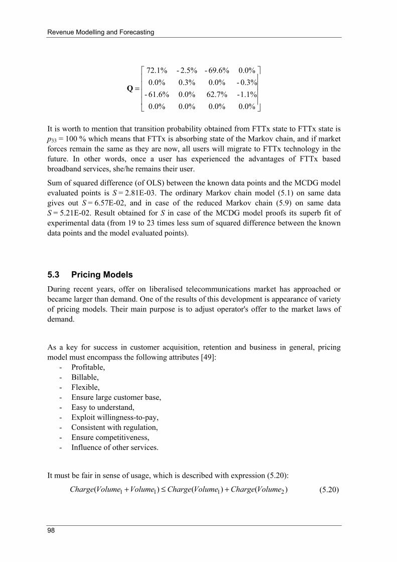
Revenue Modelling and Forecasting
98
⎥⎥⎥⎥
⎦
⎤
⎢⎢⎢⎢
⎣
⎡
=
0.0%0.0%0.0%0.0%1.1%-62.7%0.0%61.6%-0.3%-0.0%0.3%0.0%0.0%69.6%-2.5%-72.1%
Q
It is worth to mention that transition probability obtained from FTTx state to FTTx state is p33 = 100 % which means that FTTx is absorbing state of the Markov chain, and if market forces remain the same as they are now, all users will migrate to FTTx technology in the future. In other words, once a user has experienced the advantages of FTTx based broadband services, she/he remains their user.
Sum of squared difference (of OLS) between the known data points and the MCDG model evaluated points is S = 2.81E-03. The ordinary Markov chain model (5.1) on same data gives out S = 6.57E-02, and in case of the reduced Markov chain (5.9) on same data S = 5.21E-02. Result obtained for S in case of the MCDG model proofs its superb fit of experimental data (from 19 to 23 times less sum of squared difference between the known data points and the model evaluated points).
5.3 Pricing Models During recent years, offer on liberalised telecommunications market has approached or became larger than demand. One of the results of this development is appearance of variety of pricing models. Their main purpose is to adjust operator's offer to the market laws of demand.
As a key for success in customer acquisition, retention and business in general, pricing model must encompass the following attributes [49]:
- Profitable, - Billable, - Flexible, - Ensure large customer base, - Easy to understand, - Exploit willingness-to-pay, - Consistent with regulation, - Ensure competitiveness, - Influence of other services.
It must be fair in sense of usage, which is described with expression (5.20):
)()()( 2111 VolumeChargeVolumeChargeVolumeVolumeCharge +≤+ (5.20)

Revenue Modelling and Forecasting
99
Environmental variables that influence Pricing models are illustrated in Figure 5.7.
Competition
Similarservices
Regulation
Customers
Costs
PricingModel
Figure 5.7: Relation of Pricing model and environment [49]
After conception of Pricing model based on the abovementioned principles, its primary input variable is volume (traffic) of telecommunications service realised by certain user/customer in agreed time period (usually one month). Volume can be measured as one or combination of the following:
- Number of service units (e.g. number of SMS, number of IPTV premium channels, etc.);
- Duration of service usage in time units (e.g. duration of voice calls) - Realised traffic in information units (e.g. MB, GB for data service or internet
usage); - Connection speed in data transfer rate units (e.g. Mbit/s for data service or internet
usage), etc.
Moreover, pricing models can include additional attributes, such as: - Distance (e.g. different tariff for local / long-distance / international voice service;
or local / long-distance / international data lines); - Agreed level of quality of service (QoS), etc.
In continuation of this section, widespread pricing models will be presented and analysed where an operator aspect will be used, so Charge for certain telecommunication service will be denoted as Revenue.
Besides pricing model analytical characteristics, their resulting elasticises will be analysed through: Price elasticity of volume and Volume elasticity of revenue.

Revenue Modelling and Forecasting
100
Price elasticity of volume EV(p): analogue to Price elasticity of demand Ed(p) this is a measure of sensitivity of realised volume V to changes in unit price p; defined as percentage change in realised volume per percentage change in unit price:
( )
( )p
dppEVdV
dpdV
Vp
pp.p-p
VV.V-V
pE Vp-p
V ⋅=⇒⋅=
′+⋅′
′+⋅′
=→′
)(
50
50lim)(0
(5.21)
Volume elasticity of revenue ER(V): a measure of sensitivity of revenue (charge) R to changes in realised volume; defined as percentage change in revenue (charge) per percentage change in realised volume:
( )
( )VdVVE
RdR
dVdR
RV
VV.V-V
RR.R-R
VE RV-V
R ⋅=⇒⋅=
′+⋅′
′+⋅′
=→′
)(
50
50lim)(0
(5.22)
An operator expects that ER(V) is positive, i.e. that increase of realised volume has the effect on increase of revenue. A user expects that EV(p) is negative, i.e. that increase of realised volume has the effect on decrease of unit price and vice versa, which is congruent with (5.20).
5.3.1 Pricing Model: Linear without Fixed Fee
Linear without fixed fee pricing model has the following characteristics [49]: - Only pricing dimension is a per realised volume fee, - No guaranteed revenue, - Price/Volume is constant, - Linear.
Pricing model is defined with: VolumekVolumeRevenue ⋅=)( (5.23)
Analytical characteristics of Linear without fixed fee pricing model are: - Unit price is constant regarding changes in realised volume = k; - Volume elasticity of revenue is constant regarding changes in realised volume = 1; - It can be interpreted that demand for volume is perfectly elastic (EV(p) = ±∞); - It is fair in sense of usage:
)()()( 2121 VolumeRevenueVolumeRevenueVolumeVolumeRevenue +=+ (5.24)
Figure 5.8 shows Revenue -Volume and Unit price - Volume relationships and Figure 5.9 Price elasticity of volume - Volume and Volume elasticity of revenue - Volume relationships in case of this pricing model.

Revenue Modelling and Forecasting
101
0 0 Volume
Revenue(Volume) Unit price(Volume)
k
Figure 5.8: Pricing model - Linear without fixed fee
Revenue -Volume and Unit price - Volume relationships
0
1
Volume elasticity of revenue ER(V)
Volume
Figure 5.9: Pricing model - Linear without fixed fee
ER(V) - Volume relationship; EV(p) is not shown EV(p) = ±∞
5.3.2 Pricing Model: Linear with Fixed Fee
Linear with fixed fee pricing model has the following characteristics [49]: - Fixed monthly (or annual) fee plus linear charge per realised volume, - Very flexible, - Good differentiation possibilities, - Can be customised to address various segments.
Pricing model is defined with: 0;)( >+⋅= bbVolumeaVolumeRevenue (5.25)
Figure 5.10 shows Revenue -Volume and Unit price - Volume relationships and Figure 5.11 Price elasticity of volume - Volume and Volume elasticity of revenue - Volume relationships in case of this pricing model.

Revenue Modelling and Forecasting
102
0
Revenue( Volume ) Unit price( Volume )
Volume
a
b
Figure 5.10: Pricing model - Linear with fixed fee
Revenue -Volume and Unit price - Volume relationships
-1
0
1
Price elasticity of volume EV(p)Volume elasticity of revenue ER(V)
Volume
Figure 5.11: Pricing model - Linear with fixed fee ER(V) - Volume and EV(p) - Volume relationships
Analytical characteristics of Linear with fixed fee pricing model are: - Unit price decreases when volume increases approaching value of parameter a; - Volume elasticity of revenue increases when volume increases approaching 1; - Price elasticity of volume decreases when volume increases approaching value
of: - a⋅Volume / b; - It is strictly fair in sense of usage:
)()()( 2121 VolumeRevenueVolumeRevenueVolumeVolumeRevenue +<+ (5.26)
5.3.3 Pricing Model: Linear with free Trial Period
Linear with free trial period pricing model is a special case of Linear with fixed fee model, defined by (5.27) [49].

Revenue Modelling and Forecasting
103
( )⎩⎨⎧
−⋅=≥=<
=TrialVolumeaRevenueTrialVolume
RevenueTrialVolumeVolumeRevenue
0)( (5.27)
Analytical characteristics of Linear with free trial period pricing model are: - Unit price increases when volume increases approaching value of parameter a; - Volume elasticity of revenue decreases when volume increases approaching 1.
Price elasticity of volume is positive and increases when volume increases which is inconsistent with "fair in sense of usage" condition (5.20):
)()()( 2121 VolumeRevenueVolumeRevenueVolumeVolumeRevenue +>+ (5.28)
but model is favourable for users because of trial period. Figure 5.12 shows Revenue -Volume and Unit price - Volume relationships and Figure 5.13 Price elasticity of volume - Volume and Volume elasticity of revenue - Volume relationships in case of this pricing model.
0
Revenue( Volume ) Unit price( Volume )
Volume
a
Figure 5.12: Pricing model - Linear with free trial period Revenue -Volume and Unit price - Volume relationships
-1
0
1
Price elasticity of volume EV(p)
Volume elasticity of revenue ER(V)
Volume
Figure 5.13: Pricing model - Linear with free trial period
ER(V) - Volume and EV(p) - Volume relationships

Revenue Modelling and Forecasting
104
5.3.4 Pricing Model: Flat Rate
Flat rate pricing model has the following characteristics [49]: - Fee paid regardless of realised volume, - To be used by operators with utmost care, - Addresses heavy users, - No differentiation possible, - Easy to bill, - Easy to communicate, - Pricing model is defined with:
aVolumeRevenue =)( (5.29)
Analytical characteristics of Flat rate pricing model are: - Unit price decreases when volume increases approaching 0; - Volume elasticity of revenue is 0, i.e. revenue does not increase while volume
increases; - Price elasticity of volume is -1, i.e. unit (or unitary) elastic; - It is strictly fair in sense of usage:
)()()()()(
212
121
VolumeRevenueVolumeRevenueVolumeRevenueVolumeRevenueVolumeVolumeRevenue
+<===+
(5.30)
Figure 5.14 shows Revenue -Volume and Unit price - Volume relationships and Figure 5.15 Price elasticity of volume - Volume and Volume elasticity of revenue - Volume relationships in case of this pricing model.
0
Revenue(Volume) Unit price(Volume)
Volume
a
Figure 5.14: Pricing model - Flat rate
Revenue -Volume and Unit price - Volume relationships

Revenue Modelling and Forecasting
105
-1
0
1
Price elasticity of volume EV(p) Volume elasticity of revenue ER(V)
Volume
Figure 5.15: Pricing model - Flat rate
ER(V) - Volume and EV(p) - Volume relationships
5.3.5 Pricing Model: Flat Rate Cap
Flat rate cap pricing model has the following characteristics [49]: - Limits usage volume which is included in flat rate, - Beyond cap per-usage fee applies, - Limits risks of flat rate, - Addresses heavy users, - Differentiation through levels of V0, R0.
Auxiliary curve (resulting from experience learning curve [26]) determines levels of V0, R0 and slope of tangent (5.31). Auxiliary curve with two different levels for V0, R0 and corresponding tangents are shown in Figure 5.16 [62].
( ) 10;0
0 <<= bVolumeVRVolumerveAuxilaryCu b
b (5.31)
0
Auxiliary curve Revenue( Volume ) Revenue( Volume ) *
Volume V 0
R 0
R* 0
V*0
Figure 5.16: Auxiliary curve for pricing model Flat rate cap

Revenue Modelling and Forecasting
106
Pricing model is defined with:
( )⎪⎩
⎪⎨⎧
−⋅+=>
=≤=
00
000
00)( VVolume
VRbRRevenueVVolume
RRevenueVVolumeVolumeRevenue (5.32)
From (5.31) follows that for different value for volume-cap, V'0, corresponding price level R'0 should be:
b
VVRR ⎟⎟
⎠
⎞⎜⎜⎝
⎛ ′⋅=′
0
000
Increment of price ΔR per volume unit ΔV in over-cap interval follows from (5.31) and (5.32).
0
0VRbVR ⋅⋅Δ=Δ
Increment of price ΔR is lower if value for volume-cap V0 is higher - see Figure 5.16. For example, broadband internet service, chosen b = 0.67 and start package:
- Volume cap V0 = 2 GB, price R0 = 3 €, additional 1 GB of usage over cap is 1 €
generates the following additional packages:
- Volume cap V0 = 5 GB, price R0 = 5.5 €, additional 1 GB of usage over cap is 0.75 €,
- Volume cap V0 = 15 GB, price R0 = 11.5 €, additional 1 GB of usage over cap is 0.5 €, etc.
Figure 5.17 shows Revenue -Volume and Unit price - Volume relationships and Figure 5.18 Price elasticity of volume - Volume and Volume elasticity of revenue - Volume relationships in case of this pricing model.
0
Revenue( Volume ) Unit price( Volume )
Volume
R 0
0 0
V Rb ⋅
V 0
Figure 5.17: Pricing model - Flat rate cap Revenue -Volume and Unit price - Volume relationships
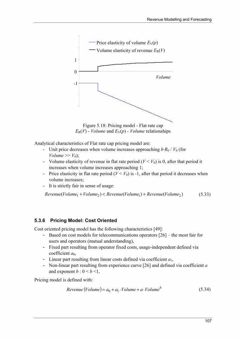
Revenue Modelling and Forecasting
107
0
1
-1
Price elasticity of volume EV(p) Volume elasticity of revenue ER(V)
Volume
Figure 5.18: Pricing model - Flat rate cap
ER(V) - Volume and EV(p) - Volume relationships
Analytical characteristics of Flat rate cap pricing model are: - Unit price decreases when volume increases approaching b·R0 / V0 (for
Volume >> V0); - Volume elasticity of revenue in flat rate period (V < V0) is 0, after that period it
increases when volume increases approaching 1; - Price elasticity in flat rate period (V < V0) is -1, after that period it decreases when
volume increases; - It is strictly fair in sense of usage:
)()()( 2121 VolumeRevenueVolumeRevenueVolumeVolumeRevenue +<+ (5.33)
5.3.6 Pricing Model: Cost Oriented
Cost oriented pricing model has the following characteristics [49]: - Based on cost models for telecommunications operators [26] – the most fair for
users and operators (mutual understanding), - Fixed part resulting from operator fixed costs, usage-independent defined via
coefficient a0, - Linear part resulting from linear costs defined via coefficient a1, - Non-linear part resulting from experience curve [26] and defined via coefficient a
and exponent b : 0 < b <1,
Pricing model is defined with:
( ) bolumeVaolumeVaaVolumeRevenue ⋅+⋅+= 10 (5.34)

Revenue Modelling and Forecasting
108
Figure 5.19 shows Revenue -Volume and Unit price - Volume relationships and Figure 5.20 Price elasticity of volume - Volume and Volume elasticity of revenue - Volume relationships in case of this pricing model.
0
Revenue(Volume) Unit price(Volume)
Volume a1 a0
Figure 5.19: Pricing model - Cost oriented
Revenue -Volume and Unit price - Volume relationships
0
Price elasticity of volume EV(p) Volume elasticity of revenue ER(V)
Volume
b
1
1−b
Figure 5.20: Pricing model - Cost oriented
ER(V) - Volume and EV(p) - Volume relationships
Analytical characteristics of Cost oriented pricing model are: - Unit price decreases when volume increases approaching value of parameter a1; - Volume elasticity of revenue increases when volume increases approaching value
of parameter b; - Price elasticity of volume decreases when volume increases to minus infinity; in
cases when a1 = 0 it is approaching value of 1/(b - 1) which is always less than -1; - It is strictly fair in sense of usage:
)()()( 2121 VolumeRevenueVolumeRevenueVolumeVolumeRevenue +<+ (5.35)

Revenue Modelling and Forecasting
109
5.3.7 Pricing Model: Volume Rounding
To cover fixed costs of production, telecom operators usually apply rounded-up billing of realised volume (traffic). Rounding principle can be mathematically noted as:
⎪⎩
⎪⎨⎧
>⎥⎥⎤
⎢⎢⎡ −⋅+
≤=
00
0
00
,
,
dVd
dVdd
dVdW (5.36)
where V is real (realised) volume (traffic), d0 is initial rounding step and d is incremental rounding step and W is billed volume (traffic) - see Figure 5.21. In expression (5.36), ceiling function is noted as ⎡x⎤.
00
W - Billed volume/traffic
d0 d0+d V - Real volume/traffic
Figure 5.21: Rounded-up billing of realised volume (traffic)
For example, in case when pricing model has for d0 = 60 seconds and d = 15 seconds, every voice call that lasts between 1 and 60 seconds will be billed as 60 seconds call. Calls that last between 61 and 75 seconds will be billed as 75 seconds call, etc. Such rounded billing is present not only in voice service, but also in (fixed and mobile) data and internet service for volumes in [MB] or [GB].
For uniformly distributed user generated volume (traffic), percentage difference between V and W can be obtained by elementary math:

Revenue Modelling and Forecasting
110
⎪⎪⎩
⎪⎪⎨
⎧
>+
−+−
≤−+
=−=2/,
)12(2)()1(2
2/,112
2
000
00
dVVV
ddddV
dVV
d
VVWε (5.37)
where W and V are average values for billed and real volume, respectively.
Specially, for d0 = 0, approximation for ε is:
0,212
10 =≅
+−= d
Vd
Vdε (5.38)
Table 5.1 presents percentage difference calculated by (5.37) for typical telecommunications services. Formula (5.37) assumes that distribution of volume (traffic) is uniform V∼U( 0 , 2V ), but in real cases it is log-normal V∼Log-N(μ,σ), which median is lower than V and consequently influence of rounding-up is higher. Therefore, values for percentage difference ε in Table 5.1 can be interpreted as minimal possible (i.e. the best case for service users / the worst case for operators).
Table 5.1: Percentage difference between realised traffic and billed traffic
Service Average
volume / traffic V
Initial rounding step d0
Incremental rounding step d
Percentage difference ε
Fixed voice 180 s 0 s 60 s + 16.3 % Fixed voice 180 s 60 s 15 s + 6.0 % Fixed voice 180 s 60 s 1 s + 2.7 %
Mobile voice 90 s 0 s 15 s + 7.7 % Mobile voice 90 s 60 s 30 s +21.5 % Mobile voice free calls with call-setup fee
180 s 60 s 0 s - 66.8 %
Broadband internet 3 GB 2 GB 1 GB + 4.8 %

Revenue Modelling and Forecasting
111
5.4 Average Revenue Per User Forecasting
Average Revenue Per User (ARPU) represents the average revenue generated per each user unit (subscriber, customer, user, fixed phone line, DSL line, SIM card, etc.) during the specified time period (monthly, quarterly and yearly). On the other side, ARPU equals to the charged (realised) volume of average user per specified time period:
( ) ( )VolumeUnitPriceVolumeVolumeChargeusersofNumber
RevenueARPU ⋅=== (5.38)
All possible cases when ARPU increases with examination of revenue, customer base and market position are presented in Figure 5.22.
Average no. of users Revenue Case / Comment
Bad for revenue and customer base
Bad for customer base
Good
Excellent
Unit price Volume Case / Comment
Good, but short-term, possible only if EV(p) ≅ 0
Good, but possible only for targeted segments where EV(p) > 0
Excellent: pricing model fits to users' needs
Bad for market share, revenue (charge) can rise only if EV(p) ∈ (-1,0)
Good for market share, revenue (charge) can rise only if EV(p) < -1
Figure 5.22: Possible cases when ARPU increases [49]
There are two basic approaches in ARPU forecasting: Top-down and Bottom-up approach.
5.4.1 Top-Down Approach
Top-down forecasting of ARPU can be done directly or indirectly based on revenue forecasting and number of users forecasting.
Direct forecasting of ARPU is possible in cases when historical time series data for ARPU have S-shaped segments, so growth models described in Chapter 4 can be used.
Indirect forecasting of ARPU in time period [t1,t2] can be calculated from (5.39):
),(),(),(
21
2121 ttN
ttRevenuettARPU =
(5.39)
The first step is revenue and number of users modelling and forecasting.

Revenue Modelling and Forecasting
112
After that, average of forecasted number of users during specified time period [t1,t2] should be calculated - see Table 5.1.
Table 5.1: Average number of users for different growth
Red line represents exact average number of uses; Grey one is a simple average between N(t1) and N(t2) [49]
Linear growth
btatN +⋅=)(
2)()()( 21
21tNtN,ttN +=
Exponential growth
0)1()()( 0ttCAGRtNtN −+⋅=
12
1221
)()()1ln(
1)(tt
tNtNCAGR
,ttN−−⋅
+=
Logistic growth )( 01)( ttae
MtN −−+=
⎥⎦
⎤⎢⎣
⎡⋅
−−⋅=
)()(ln
)(11)(
1
2
1221 tN
tNtta
M,ttN
In general, ARPU obtained by top-down approach is a useful benchmark for the bottom-up approach (sanity check).
5.4.2 Bottom-Up Approach
ARPU in time period [t1,t2] can be calculated from the forecasts of the lowest-level disaggregate forecasts about service usage (volume) for all recognised market segments and forecasts about appropriate/affordable pricing models related to recognised market segments. Steps in bottom-up ARPU forecasting (Figure 5.23) are:
- Estimation of typical service usage (volume) for recognised segments according to users' life-styles;
- Determination of appropriate/affordable pricing model;
- Price trends assumption based on external influences (e.g. price erosion);
- Obtaining Average Revenue per User.
Based on Pricing Models described in section 5.3, expression (5.40) can be used for bottom-up ARPU calculation.
∑=
⎥⎦⎤
⎢⎣⎡ +⋅=
n
iiii
ttttUsagePricefttARPU1
212121 2),,(),( (5.40)
where fi are segments share (5.41), defined via number of users in i-segment Ni:

Revenue Modelling and Forecasting
113
∑=
==n
ii
tot
ii f
NNf
1
%100; (5.41)
Service usage
distrib.Se
gmen
ts1,
2, .
.. n
Pricing models∼ Usage
Price trend ∼ Time /
penetration
. . . . . . . . .
f1
f2
. . .
fn
Seg-ment share
Figure 5.23 Steps in bottom-up ARPU forecasting [49]
Function Price (Usage, Time) in 5.40 is based on pricing models described in section 5.3, but it encompasses price trend in the future. Usually, service price erosion could be expected in the future due to strong telecommunications equipment price erosion trend and competitive conditions on liberalised markets.
Price drop dynamics can be related with penetration level in future or simply time dependent.
In case of time dependent price erosion, it usually follows declining exponential model (5.42):
( ) ( )( )01Pr YearYearaYearice −−= (5.42)
where a is annual rate of decrease, 0 < a < 1.

Integration of Analytical Method
114
6 Integration of Analytical Method
Integration of all forecasting modules is presented in Tables 6.1 - 6.3. First table presents User growth dynamics forecasting module, the second Revenue forecasting module and the third module with elements for Improvement of forecasting quality.
Most right cells represent models and procedures that support specific forecasting needs. Numbers in square brackets represent related sections in Thesis.
Table 6.1: User growth dynamics forecasting module
Logistic Growth Model [3.3]
Logistic Model through Two Fixed
Points [3.3.1], [4.1.1.1]
Logistic Model through One Fixed
Point [3.3]
Imitation prevails Logistic Growth Model
based
Logistic model through three points
[4.1.1.2] Bass Model [3.4] Bass Model with
Explanatory Parameters [4.1.6] Innovation and imitation
Bass model based Bass Model Through One Fixed Point
[4.1.7] Richards Model [3.5]
Growth Models for the First Segment of Service Life-
Cycle
Imitation prevails with flexible inflexion
Richards Model based
Richards Model through One Point
[4.1.4] Growth Models for the First Segment and Successive
Segments of Service Life-Cycle
Generalisation of Recursive Growth Models [4.1.10]
Monotone growth/decline Logistic Spline Model [4.2.1] Growth Models for
Successive Segments of
Service Life-Cycle General case of
successive segments
Universal Model for Successive Segments of Service Life-Cycle
[4.2.2]
User growth dynamics
forecasting
Growth Models for whole Service Life-
Cycle
Multi-Logistic Model [4.3.1]

Integration of Analytical Method
115
Table 6.2: Revenue forecasting module
Overall Modelling of Market Share by Markov Chains [5.2.2] Market Share
Modelling and Forecasting Markov Chains Based on Diffusion Growth
Model Principles [5.2.3] Pricing Model: Linear without Fixed Fee
[5.3.1] Pricing Model: Linear with Fixed Fee
[5.3.2] Pricing Model: Linear with free Trial Period
[5.3.3] Pricing Model: Flat Rate
[5.3.4] Pricing Model: Flat Rate Cap
[5.3.5] Pricing Model: Cost Oriented
[5.3.6]
Pricing Models
Pricing Model: Volume Rounding [5.3.7]
Top-Down Approach [5.4.1]
Revenue forecasting
Average Revenue Per User Forecasting Bottom-Up Approach
[5.4.2]
Table 6.3: Module for improvement of forecasting quality
Uncertainty of Forecasted Service Market Capacity
Direct procedure based on Logistic model through three points [4.1.2]
Statistical Laws of New Technologies and New Services Roll-Out [4.4.1]
Statistical Laws of Market Segments [4.4.2]
Forecasting quality
improvement Experiences from Telecommunications
Operations
Statistical Laws of Usage Segmentation [4.4.3]

Conclusions
116
7 Conclusions According to the forecasting praxis and academic research in a field of forecasting in telecommunications business, optimal results can be obtained by combination of qualitative and quantitative methods. However, the existing quantitative time series forecasting methods are based on analytical models with limited ability to accept results of qualitative forecasting as external variables or model parameters.
Forecasting of service market adoption through growth of users is examined in two ways: adoption of a new service in first segment of service life-cycle and adoption of the existing service during later segments of service life-cycle.
In case of new service market adoption (first phase of service life-cycle), an example of successful qualitative - quantitative integration is the logistic model through two fixed points, but due to limits of the logistic model it has restricted usage. Based on the analysis of existing growth models and the abovementioned requirements, the Bass model with explanatory parameters was developed, suitable for forecasting prior to service launch or in early phases of the service life-cycle. In addition, the Richards model is modified based on same principle that was used for the logistic model. The Bass with explanatory parameters and the modified Richards model are suitable for forecasting of all conditions for new service market adoption.
In case of existing service market adoption (later phases of service life-cycle) three different models were developed depending on forecasting needs and available inputs:
Logistic spline model
The Logistic spline model is suitable for forecasting of service life-cycle segments with monotone growth or decline. Moreover, the logistic spline can recognise and warn that qualitative forecasting inputs (assumptions) are inadequate.
Universal Model for Successive Segments of service life-cycle
The Universal model for successive segments has been developed for most often case: modelling for current market adoption segment and the first successive segment in the future. Namely, a forecaster practitioner can anticipate one consecutive part of market adoption segment in the future and has available only limited input data set.
Multi-logistic model
The Multi-logistic model can model market adoption of service during the entire service life-cycle, but requires large set of known data points, which limits its application for the forecasting purposes.
Issue of uncertainty and sensitivity on input data is analysed on case of the logistic model. Procedure for direct assessment of logistic model sensitivity to uncertainty of input data has been developed. Results show that uncertainty of obtained market capacity only depends on measurement error of input data and known penetration range that is covered by input data.

Conclusions
117
Based on experience and available data form telecommunications operations statistical laws and regularities are recognised and modelled to provide forecasting inputs that were not directly accessible. Focus was on new technologies and new services roll-out performance and analysis of market (sub)segment values.
Revenue forecasting is given in systematised way incorporating all its elements: market share modelling, pricing models and average revenue per user modelling. It is suggested to use top-down and bottom-up approach simultaneously which enables mutual sanity check.
For the overall modelling of market share, the new concept of Markov chains based on diffusion growth model principles has been developed. It is suitable for modelling of diffusion of new technology and telecommunications services for the whole service life-cycle where interactions with different operators or technology are evident. The model can give early warning for service operators to change their market performance right on time.
Integration of all analysed and developed models and forecasting procedures in analytical method has been done with appropriate flow chart depending on specific forecasting needs.
Future work
During preparation of the Thesis, a number of interesting research challenges has been identified for the future work. They can be divided into: growth model improvement, quality of forecasting improvement and modelling of revenue elements.
The main challenges in field of growth model improvement are concretisation of conditions on the Generalised recursive growth models and finding its explicit forms for specific cases.
The main challenges in field of forecasting quality improvement are further investigations of features of the Universal model for successive segments related to enabling warning that qualitative forecasting inputs (assumptions) are inadequate. In addition, further research regarding analysis of uncertainty and sensitivity on input data for modelling of later phases of service life-cycle.
New concept of the Markov chains based on diffusion growth model gives principles for developing of the Markov based model for average revenue per user and its forecasting.

Appendix
118
Appendix List of Techno-economic indicators in telecommunications business
1. Indicators and definitions of WirelessIntelligence on-line business intelligence database (https://www.wirelessintelligence.com/index.aspx, visited on 2009-03-29)
CONNECTIONS
Number of Connections
A SIM, or where SIMs do not exist, a unique mobile telephone number, which has access to the network for any purpose (including data only usage) except telemetric applications
Total, Contract, Prepaid, cdmaOne, CDMA2000 1X, CDMA2000 1xEV-DO, GSM, WCDMA, TDMA, PDC, iDEN, Analog
Current rank by Connections
Total (Country), Total (Region), Total (World), cdmaOne (Country), cdmaOne (Region), cdmaOne (World), CDMA2000 1X (Country), CDMA2000 1X (Region), CDMA2000 1X (World), CDMA2000 1xEV-DO (Country), CDMA2000 1xEV-DO (Region), CDMA2000 1xEV-DO (World), GSM (Country), GSM (Region), GSM (World), WCDMA (Country), WCDMA (Region), WCDMA (World), TDMA (Country), TDMA (Region), TDMA (World), PDC (Country), PDC (Region), PDC (World), iDEN (Country), iDEN (Region), iDEN (World), Analog (Country), Analog (Region), Analog (World)
Market Share of Connections
Operator connections divided by total connections for the country, shown as a percentage.
Total, cdmaOne, CDMA2000 1X, CDMA2000 1xEV-DO, GSM, WCDMA, TDMA, PDC, iDEN, Analog
Growth Rate, Connections (Sequential)
Connections in current quarter divided by connections in previous quarter shown as a percentage
Total, cdmaOne, CDMA2000 1X, CDMA2000 1xEV-DO, GSM, WCDMA, TDMA, PDC, iDEN, Analog
Growth Rate, Connections (Year on year)
Connections in current quarter divided by connections in relevant quarter a year previously shown as a percentage
Total, cdmaOne, CDMA2000 1X, CDMA2000 1xEV-DO, GSM, WCDMA, TDMA, PDC, iDEN, Analog
% of Connections
The number of connections in the relevant technology divided by the total connections for the given
Contract, Prepaid, cdmaOne, CDMA2000 1X, CDMA2000 1xEV-DO, GSM, WCDMA, TDMA, PDC, iDEN, Analog

Appendix
119
operator, expressed as a percentage.
Market Penetration
Number of connections divided by Population Total
Net Additions Connections in this quarter minus connections in the previous quarter.
Total, cdmaOne, CDMA2000 1X, CDMA2000 1xEV-DO, GSM, WCDMA, TDMA, PDC, iDEN, Analog
Market Share - Net Additions
Operator net adds divided by total net adds for the country, shown as a percentage
Total, cdmaOne, CDMA2000 1X, CDMA2000 1xEV-DO, GSM, WCDMA, TDMA, PDC, iDEN, Analog
Gross Additions Net additions + Disconnections Total
Disconnections Average number of connections in the period * monthly churn * 3
Total
OPERATIONAL
Churn
Total gross customer disconnections (voluntary or involuntary) in the period divided by the average total customers in the period. The Figure is expressed monthly, whereby if an operator reports annual churn, Wireless Intelligence divides this reported number by 12 to get a monthly equivalent.
Total, Contract, Prepaid
Minutes of Use per User
Total minutes used in the period (outgoing calls, incoming calls and roaming) divided by the weighted average number of customers over the same period, expressed monthly.
Total, Contract, Prepaid
Minutes Of Use Total
Average number of connections in the period * MoU per user per month * 3 Total
Effective Price Per Minute ARPU / Minutes of Use per user per month Total
ARPU
Total recurring revenue divided by the weighted average number of customers during the same period. The Figure is expressed monthly, whereby if an operator reports annual ARPU, Wireless Intelligence divides this reported number by 12 to get a monthly equivalent.
Total, Contract, Prepaid, Voice, Non-Voice
Current rank by ARPU
Total (Country), Total (Region). Total (World)
Subscriber Acquisition Costs per user
The total of connection fees, trade commissions and equipment costs, net of related revenue, relating to new customer connections.
Total, Contract, Prepaid
Total Billed SMS events Total
SMS Messages per User per Month
Total

Appendix
120
FINANCIAL
Total operator reported revenue, includes all recurring and non-recurring revenues. Total
Revenues from generated by the use of the wireless network (i.e. excluding handset revenue and connection fees). Commonly includes voice, data and messaging and includes the traffic generated by the operator’s subscribers and the traffic generated by the other operators.
Recurring
Recurring revenue attributable to voice transmission and any appropriate monthly charges. Voice
Recurring revenue attributable to non-voice services and any appropriate monthly charges. Commonly includes text and multimedia messaging, data transmission, downloads, Internet browsing and other data services.
Non-Voice
Revenue
All revenue reported that is excluded from recurring revenue. Commonly includes revenue from equipment. Non-Recurring
Current rank by Revenue
Total (Country), Total (Region), Total (World)
Operating Expenditure Simple measure of Opex: Recurring Revenue - EBITDA Total
Opex / Revenue - Rolling 12 month
Rolling 12 month Opex / Rolling 12 month total revenues, converted at historic currency. Total
Operating Free Cash Flow Simple measure of Free Cash Flow: EBITDA - Capex Total
Data as Percentage of Service Revenue
Non-voice revenues divided by recurring revenues, expressed as a percentage. Total
CAPEX Capital expenditures in tangible and intangible assets excluding licenses. Total
Capex / Revenue - Rolling 12 month
Rolling 12 month capex / Rolling 12 month total revenues, converted at historic currency. Total
EBITDA Total
EBITDA margin Operating profit before depreciation, amortisation, profit or loss on disposal of fixed assets and exceptional items expressed as a percentage of total turnover.
Total

Appendix
121
2. List of definitions and indicators from World Telecommunication/ICT Indicators 2008 database (http://www.itu.int/ITU-D/ict visited on 2009-03-29)
1. Basic indicators
The data for Population are mid-year estimates from national statistical offices or the United Nations (UN). Population Density is based on land area data from the UN; the land area does not include any overseas dependencies but does include inland waters. The data for Gross Domestic Product (GDP) are generally from the IMF. They are current price data in national currency converted to United States dollars by the method identified above. Total telephone subscribers refer to the sum of main telephone lines and cellular mobile subscribers (see below for definitions). Total telephone subscribers per 100 inhabitants is calculated by dividing the total telephone subscribers by the population and multiplying by 100. Effective teledensity is the higher value of either main telephone lines per 100 inhabitants or mobile cellular subscribers per 100 inhabitants.
2. Main telephone lines
This table shows the number of Main telephone lines and Main telephone lines per 100 inhabitants for the years indicated and corresponding annual growth rates. Main telephone lines refer to telephone lines connecting a customer's equipment (e.g., telephone set, facsimile machine) to the Public Switched Telephone Network (PSTN) and which have a dedicated port on a telephone exchange. Note that for most countries, main lines also include public payphones. Many countries also include ISDN channels in main lines (see 9. ISDN and ADSL). Main telephone lines per 100 inhabitants is calculated by dividing the number of main lines by the population and multiplying by 100.
3. Waiting list
The table shows the total number of applications for a connection to a main telephone line that have had to be held over owing to a lack of technical availability. It should be noted that the waiting list refers to applications received; it does not include figures for those who desire a telephone line but have not submitted an application. Total demand is obtained by adding main lines in operation and the waiting list. Satisfied demand is obtained by dividing the number of main lines by the total demand for main telephone lines (sum of the unmet applications and operating main telephone lines). Waiting time shows the approximate number of years applicants must wait for a telephone line. It is calculated by dividing the number of applicants on the waiting list by the average number of main lines added per year over the past three years.
4. Local telephone network
Capacity used is obtained by dividing the number of main lines in service by the total number of main lines that could be connected to local public switching exchanges. The Automatic per cent is calculated by dividing the number of main lines connected to automatic exchanges by the total number of main lines. The Digital per cent is calculated by dividing the number of main lines connected to digital exchanges by the total number of main lines. The percentage of Residential lines refers to the number of main lines serving households (i.e. lines that are not used for professional purposes or as public telephone stations) divided by the total number of main lines. Faults per 100 main lines per year refer to the number of reported faults per 100 main telephone lines for the year indicated. It is calculated by the total number of reported faults for the year divided by the number of telephone main lines and multiplied by 100. Some countries report this

Appendix
122
on a monthly basis, so an annual estimate is made by multiplying by 12. The definition of a fault varies among countries: some operators define faults as including malfunctioning customer equipment while others include only technical faults.
5. Teleaccessibility
Total residential main lines refer to the number of main lines used by households. Per 100 households is obtained by dividing the number of residential main lines by the number of households and multiplying by 100. Payphones refers to the total number of all types of public telephones including coin- and card-operated ones. Some countries include public phones installed in private places. No distinction is made between operational and non-operational payphones. Per 1000 inhabitants is obtained by dividing the number of public payphones by the population and multiplying by 1000. As % of main lines is obtained by dividing the number of public telephones by the number of main lines.
6. Telephone tariffs
The table shows the costs associated with local residential and business telephone service. Connection refers to connection charges for basic telephone service. Monthly subscription refers to the recurring fixed charge for subscribing to the PSTN. This indicator is not always comparable since some countries include a number of free local calls in the subscription. When subscription charges are reported annually or bi-monthly, they are converted to their corresponding monthly amount. Local call refers to the cost of a 3-minute call within the same exchange area using the subscriber's equipment (i.e., not from a public telephone). This is the amount the subscriber must pay for a 3-minute call and not the average price for each 3-minutes. Any taxes involved in these three charges are included to improve comparability. The Subscription as a % of GDP per capita shows cost of an annual residential telephone subscription as a percentage of Gross Domestic Product (GDP) per capita.
7. Mobile cellular subscribers
Mobile cellular telephone subscribers refer to users of portable telephones subscribing to an automatic public mobile telephone service using cellular technology that provides access to the PSTN. Per 100 inhabitants is obtained by dividing the number of cellular subscribers by the population and multiplying by 100. Prepaid subscribers refers to the total number of mobile cellular subscribers using prepaid cards. Population coverage measures the percentage of inhabitants that are within range of a mobile cellular signal whether or not they are subscribers. This is calculated by dividing the number of inhabitants within range of a mobile cellular signal by the total population. As a % of total telephone subscribers is obtained by dividing the number of cellular subscribers by the total number of telephone subscribers (sum of the main telephone lines and the cellular subscribers.
8. Prepaid cellular tariffs
Connection charge refers to the initial, one-time charge for a new subscription. Per minute local call refers to the average cost of a one-minute peak and off-peak rate mobile local to within the same network. When there are different rates, the price of a call to the same mobile network is used. Cost of local SMS is the price of sending a national Short Message Service (SMS) message from a mobile handset within the same network. 100 minutes of use includes the tariff components of 50 minutes of local peak time calling and 50 minutes of local off-peak calling. Differences in the distance of calls, which may be applicable in some countries, are not taken into account, nor are international calls or SMS messages. The possible onetime charge for connection is not taken into account, except where this is bundled into the costs of a prepaid account. The price comparison is

Appendix
123
expressed in US$, and as a percentage of per capita income, which is computed by dividing the 100 minutes of use by the Gross National Income (GNI) of the country.
9. ISDN and ADSL
ISDN subscribers refers to the number of subscribers to Integrated Services Digital Networks. It includes both basic rate and primary rate interface subscribers. B-channel equivalents converts the number of ISDN subscriber lines into their equivalent voice channels. The number of basic rate subscribers is multiplied by two and the number of primary rate subscribers is multiplied by 23 or 30 depending on the standard implemented. B-channels per 1000 inhabitants is the number of B-channel equivalents divided by the population and multiplied by 1000. B-channels as % of main lines is the number of B-channel equivalents divided by the number of main telephone lines. DSL subscribers refers to subscribers using Digital Subscriber Line (DSL) technology. DSL is a technology for bringing high-bandwidth information to homes and small businesses over ordinary copper telephone lines, with speed equal to, or greater than 256 kbit/s, as the sum of the capacity in both directions. As % of subscriber lines is calculated by dividing the number of DSL subscribers by the number of subscriber lines. Subscriber lines is calculated by subtracting the number of ISDN channels from main telephone lines and adding ISDN subscribers.
10. International telephone traffic
Outgoing international telephone traffic refers to total telephone traffic measured in minutes that originated in the specified country with a destination outside the country. As % of bothway refers to outgoing traffic divided by total traffic (incoming and outgoing). Minutes per inhabitant is obtained by dividing outgoing international minutes by the number of inhabitants in the country. Minutes per subscriber is obtained by dividing outgoing international minutes by the number of main lines. International telephone circuits refers to the number of links (voice channel equivalents) with other countries for establishing telephone communications.
11. Telecommunication staff
Telecommunication staff refers to the total number of staff (part-time staff converted to full-time equivalents) employed by telecommunication enterprises providing public telecommunication services. In some cases where posts and telecommunication organisations are combined, no breakdown of telecommunication staff is available. Note that the figure would generally not include sub-contract staff. % female refers to the number of full time telecommunication staff that are female divided by the total number of employees. Main lines per employee is computed by dividing the number of main lines by the number of employees. Caution should be used in interpreting this figure as some countries may subcontract a proportion of work, in which case the number of main lines per employee would be overstated.
12. Telecommunication revenue
This table shows the revenues (turnover) received from providing telecommunication services in each country. United States dollar values are obtained by the method described earlier. Data may not be strictly comparable due to a number of factors. First, it is assumed that the data relate to revenues of all operators providing service in the country. This is not unequivocally known and may be impossible to determine since there may be no legal requirement for all operators to provide financial information, or operators may be part of a parent company that only provides consolidated accounts. The data does not always include revenues from cellular mobile telephone, radio paging or data services in some developing nations if these services are not provided by the main fixed-link operator. Second, the operators may have subsidiaries with financial activities unrelated to telecommunication services that may be included. Third, in the case of countries where

Appendix
124
posts and telecommunications are combined, a perfect allocation of revenues is not always possible. Fourth, there are definition and accounting differences among countries. Total telecommunication revenue consists of all telecommunication revenues earned during the financial year under review. % mobile revenue is the share of mobile communication revenue. Per inhabitant shows current revenues divided by the number of inhabitants in the country. Per telephone subscriber is obtained by dividing revenues by total telephone subscribers (fixed plus mobile). Per employee is obtained by dividing revenues by employees. For some countries, no breakdown between postal and telecommunication staff is available and the figure may thus be unrealistically low. As a % of GDP shows telecommunication revenues divided by national Gross Domestic Product.
13. Telecommunication investment
Investment refers to the annual expenditure associated with acquiring ownership of property and plant used for telecommunication services and includes land and buildings. Total telecom investment shows total current investments for the year indicated; the United States dollar figure is arrived at by the method described above. Per inhabitant is obtained by dividing the annual investment by the population. Per telephone subscriber is obtained by dividing investment by total telephone subscribers (fixed plus mobile). As a % of revenue is obtained by dividing annual investment by telecommunication revenues. As a % of GFCF shows telecommunications investment divided by Gross Fixed Capital Formation (GFCF). For some countries where GFCF is not available, Gross Domestic Investment is used. This is similar to GFCF except that it does not include changes in inventories that tend to comprise a small proportion of GFCF.
14. Information technology
Internet subscribers refers to the number of dial-up, leased line and broadband Internet subscribers. Internet subscribers per 100 inhabitants is obtained by dividing the number of subscribers by the population and multiplied by 100. Internet Users is based on nationally reported data. In some cases, surveys have been carried out that give a more precise figure for the number of Internet users. However surveys differ across countries in the age and frequency of use they cover. The reported figure for Internet users – which may refer to only users above a certain age – is divided by the total population and multiplied by 100 to obtain users per 100 inhabitants. Countries that do not have surveys generally base their estimates on derivations from reported Internet Service Provider subscriber counts, calculated by multiplying the number of subscribers by a multiplier. PCs shows the estimated number of Personal Computers (PCs), both in absolute numbers and in terms of PCs per 100 inhabitants. The figures for PCs come from the annual questionnaire supplemented by other sources.
15. Internet
Internet subscribers refers to the number of dial-up, leased line and broadband Internet subscribers. Broadband subscribers refer to the sum of DSL, cable modem and other broadband subscribers. Although there exist various definitions of broadband, it may be defined as sufficient bandwidth to permit combined provision of voice, data and video. Speed should be greater than 128 kbps in at least one direction. As % of total subscribers is calculated by dividing the total number of broadband subscribers by the total number of Internet subscribers. Subscribers per 1000 inhabitants is calculated by dividing the number of broadband subscribers by population of the country multiplied by 1000. International bandwidth refers to the amount of international Internet bandwidth measured in Mega Bits Per Second (Mbps). Data for Internet bandwidth come from ITU’s annual questionnaire supplemented with data from TeleGeography. Bits per inhabitant is calculated by dividing the international Internet bandwidth by the population.

Appendix
125
16. Internet tariffs
The table shows the costs associated with 20 hours dial-up use per month. If broadband prices are cheaper, these are used instead. Data are generally those of the largest Internet Service Provider (ISP) and incumbent telephone company as they list the prices. ISP charge refers to the Internet monthly subscription plus extra charges once free hours have been used up. Telephone charge refers to the amount payable to the telephone company for local telephone charges while logged on. This includes usage charges but does not include the telephone line rental. Total Internet price refers to the sum of telephone usage charges and ISP charges. As % of GNI per capita shows cost of 20 hours use per month as a percentage of Gross National Income (GNI).
17. Multichannel TV
Cable TV subscribers are those who subscribe to a multi-channel television service delivered by a fixed-link connection, usually coaxial or fibre optic cable. However, some countries also report subscribers using wireless technology. In addition, some countries also report the number of households cabled to community antenna systems re-broadcasting free-to-air channels because of poor reception. As % of TV households is calculated by dividing the number of cable TV subscribers by the number of TV households. Home satellite antennas shows the number of households with access to a multi-channel television service delivered by satellite. This figure includes both Direct-to-the-home (DTH) service and Satellite Master Antenna Television (SMATV) which serves several households in the same building. SMATV serving households in different buildings is counted as cable TV. Cable modem Internet subscribers refer to Internet subscribers via a cable TV network. As % of cable TV subscribers is calculated by dividing the number of cable modem Internet subscribers by the total cable TV subscribers and multiplying by 100.
18. Network growth
This table shows the increase in the number of main telephone lines, mobile cellular subscribers and Internet users over the preceding year. Note that particularly for main telephone lines, the figure is the addition to the base of main lines and does not reflect replacements.
List of indicators:
% automatic main lines Business telephone connection charge (US$) % digital main lines Business telephone monthly subscription (US$) % of homes with a Personal Computer Consumer price index (1995=100)
% of homes with Internet Coverage of mobile cellular network (population, in %)
% of households with a radio Faults per 100 main (fixed) lines per year % of households with a telephone Fixed telephone service investment (US$) % of households with a television Gross domestic product (GDP) (US$) % of main lines in urban areas Gross Fixed Capital Formation (GFCF) (US$) % of telephone faults cleared by next working day Home satellite antennas % residential main lines Households

Appendix
126
(List of indicators - cont.)
International incoming fixed telephone traffic (calls) Number of national (fixed) long distance
telephone (calls) International incoming fixed telephone traffic
(minutes) Number of national (fixed) long distance telephone (minutes)
International Internet Bandwidth (Mbps) Personal computers International Internet Bandwidth per inhabitant
(bit/s) Personal computers per 100 inhabitants
International outgoing fixed telephone traffic (calls) Population
International outgoing fixed telephone traffic (minutes) Population - Urban population (%)
International telephone circuits Population of largest city
Internet subscribers (Cable modem ) Price of a 3-minute fixed telephone local call (off-peak rate - US$)
Internet subscribers (Dial-up) Price of a 3-minute fixed telephone local call (peak rate - US$)
Internet subscribers (DSL) Public payphones Internet subscribers (Total fixed broadband) Public payphones per 1000 inhabitants Internet subscribers (Total fixed broadband) per
100 inhabitants Radio equipped households
Internet subscribers (Total fixed Internet) Radio sets Internet subscribers (Total fixed) per 100
inhabitants Residential monthly telephone subscription (US$)
Internet users (Estimated) Residential telephone connection charge (US$) Internet users per 100 inhabitants Revenue from fixed telephone service (US$) ISDN Channels Revenue from mobile communication (US$) ISDN subscribers Staff (Female telecommunication staff) Main (fixed) telephone lines in largest city Staff (Total full-time telecommunications staff) Main (fixed) telephone lines in operation Telecommunication equipment (Export) (US$) Main (fixed) telephone lines per 100 inhabitants Telecommunication equipment (Import) (US$) Mobile cellular - price of 3-minute local call (off-
peak - US$) Television equipped households
Mobile cellular - price of 3-minute local call (peak - US$) Television receivers
Mobile cellular connection charge (US$) Television receivers per 100 inhabitants Mobile cellular monthly subscription (US$) Television subscribers (cable) Mobile cellular telephone subscribers - (Post-paid
+ Pre-paid) Total annual investment in telecom (US$)
Mobile cellular telephone subscribers - prepaid subscribers Total capacity of local public switching
exchanges Mobile cellular telephone subscribers (Digital) Total national (fixed) telephone traffic (calls) Mobile cellular telephone subscribers per 100
inhabitants Total national (fixed) telephone traffic (minutes)
Mobile communication investment (US$) Total revenue from all telecommunication services (US$)
Mobile communications staff Total telephone subscribers (fixed + mobile)
Number of local (fixed) telephone (calls) Total telephone subscribers (fixed + mobile) per 100 inhabitants
Number of local (fixed) telephone (minutes) Waiting list for main (fixed) lines

References
127
References
[1] Armstrong, J. S. (Eds), Principles of Forecasting: A Handbook for Researchers and Practitioners, Kluwer Academic Publishers, 2001
[2] Armstrong, J. S., Forecasting principles Methodology Tree, http://www.forecastingprinciples.com/methodologytree.html; visited: 2009-03-29
[3] Armstrong, J. S., Questions regarding forecasting Methodology tree (personal email), received: 2009-03-17
[4] Sokele, M., V. Hudek, Extensions of logistic growth model for the forecasting of product life cycle segments, Advances in Doctoral Research in Management Vol. 1 (ed. L. Moutinho), World Scientific Publishing, 2006, pp 77-106
[5] Sokele, M., V. Hudek, A.-I. Mincu; Opportunities for Implementation Machine-to-Machine Services via 3G Mobile Networks, Proceedings of the 7th International Conference on Telecommunications ConTEL 2003, Zagreb 2003.
[6] Fildes R., V. Kumar, Telecommunications demand forecasting a review, International Journal of Forecasting, Volume 18, Issue 4, 2002
[7] Gordon, T. J., The Delphi Method, Futures Research Methodology http://www.gerenciamento.ufba.br/Downloads/delphi%20(1).pdf ; visited: 2009-03-29
[8] Gardner, M., Practical Applications of Forecasting, Proceedings of Telecoms Forecasting Masterclass, IBC, London 2002
[9] Makridakis, S., S. Wheelwright, R. Hyndman, Forecasting: Methods and Applications (3rd edition), Wiley, 1998
[10] Albright, R. E., What Can Past Technology Forecasts Tell Us About the Future?, Technological Forecasting and Social Change, 69(5), 443-464.
[11] Lemos, A. D., A. C. Porto, Technological Forecasting Techniques and Competitive Intelligence: Tools for Improving the Innovation Process, Industrial Management and Data Systems, 98(7-8), 330-337.
[12] Bers, J. A., B. S. Lynn, C. Spurling, A computer Simulation Model for Emerging Technology Business Planning and Forecasting, International Journal of Technology Management, 18(1-2), 31-45.
[13] Zhu, D. H., A. L. Porter, Automated Extraction and Visualisation of Information for Technological Intelligence and Forecasting, Technological Forecasting and Social Change, 69(5), 495-506.
[14] Kayal, A., Measuring the Pace of Technological Progress: Implications for Technological Forecasting, Technological Forecasting and Social Change, 60(3), 237-245.

References
128
[15] Bass, F., K. Gordon, T. L. Ferguson, M. L. Githens, DIRECTV: Forecasting Diffusion of a New Technology prior to Product Launch, Interfaces, 31(3), S82-S93.
[16] Meade, N., T. Islam, Technological Forecasting Model Selection, Model Stability, and Combined Models, Management Science, 44(8), 1115-1130.
[17] Fildes, R., V. Kumar, Telecommunications Demand Forecasting - A Review, International Journal of Forecasting, 18 (2002) 489-522.
[18] Chang, P. T., C. H. Chang, A Stage Characteristic - Preserving Product Life Cycle Modelling, Mathematical and Computer Modelling, 37(12-13), 1259-1269.
[19] Funk, J. L., The Product Life Cycle Theory and Product Line Management: the Case of Mobile Phones, IEEE Transactions on Engineering Management, 51(2), 142-152.
[20] Werker, C., Innovation, Market performance, and Competition: Lessons from a product Life Cycle Model, Technovation, 23(4), 281-290.
[21] Karlsson, C., K. Nystrom, Exit and Entry Over the Product Life Cycle: Evidence From the Swedish Manufacturing Industry, Small Business Economics, 21(2), 135-144.
[22] Bass, P. I, F. M. Bass, Diffusion of Technology Generations: A Model of Adoption and Repeat Sales, Working paper, Bass Economics.
[23] Meade, N., T. Islam, Modelling and forecasting the diffusion of innovation - A 25-year review, International Journal of Forecasting, Vol 22, No. 3 (2006), pp 519-545
[24] Sokele, M., Growth models for the forecasting of new product market adoption, Telektronikk 3/4, 2008.
[25] Meyer S. P., J. H. Ausubel, Carrying Capacity: A Model with Logistically Varying Limits, Technological Forecasting and Social Change, 61(3):209-214, 1999.
[26] Stordahl, K., Long-term telecommunication forecasting (Ph.D. thesis), Norwegian University of Science and Technology, Trondheim, 2006.
[27] Meade, N., A Modified Logistic Model Applied to Human Populations, Journal of the Royal Statistical Society, Series A (Statistics in Society), Vol. 151, No. 3 (1988), pp 491-498
[28] Bass, F., A new product growth for model consumer durables, Management Science 15 (5): 215-227, 1969
[29] Bass, P. I., F. M. Bass, IT waves: two completed generational diffusion models, Working Paper, www.basseconomics.com
[30] Lilien, G. L., A. Rangaswamy, C. Van den Bulte, Diffusion Models: Managerial Applications and Software, New-Product Diffusion Models pp. 295-336, Kluwer Academic Publishers, 2000.
[31] Norton, J. A., F. M. Bass, A diffusion theory model of adoption and substitution for successive generations of high technology products. Management Science, 33, 1069– 1086.

References
129
[32] Richards, F. J., A flexible growth curve for empirical use, J. Exp. Bot., 10, 290-300, 1959.
[33] Mahajan, V., E. Muller, F. M. Bass, New product diffusion models in marketing: A review and directions for research, Journal of Marketing, 54, 1-26
[34] Meyer, P., Bi-Logistic Growth, Technological Forecasting and Social Change, 47:89-102 (1994)
[35] Sokele, M., V. Brlić, V. Hudek: Using Logistic Splines for the Prediction of Telecommunications Service Penetration over Time, Proc. of the Telecoms Forecasting Conference, IBC, London, 2002.
[36] Modis, T., Conquering Uncertainty: Understanding Corporate Cycles and Positioning Your Company to Survive the Changing Environment, Business Week Books (McGraw-Hill), New York, 1998.
[37] Debecker, A., T. Modis, Determination of the Uncertainties in S-Curve Logistic Fits, Technolog1cal Forecasting and Social Change, 46,153-17 (1994)
[38] Sokele, M., Uncertainty of forecasted new service market capacity obtained by logistic model, Proc. of the 28th International Symposium on Forecasting, Nice, 2008.
[39] Mihoković, Ž., Tržište elektroničkih komunikacija Republike Hrvatske u novom regulatornom okruženju (HAKOM), Zbornik radova Telecom Arena, 2009
[40] Wireless intelligence - Business Intelligence on-line database, https://www.wirelessintelligence.com, visited: 2009-03-29
[41] Giovanis, A. N., C. H. Skiadas, A new modeling approach investigating the diffusion speed of mobile telecommunication services in EU-15, Computational Economics, 29 (2), 2007
[42] Sokele, M., Determining how to optimise data quality and analysis to ensure precise forecasts, Proceedings of IIR Telecoms Market Forecasting Conference, 2008
[43] World Telecommunication/ICT Indicators 2008 database, http://www.itu.int/ITU-D/ICT, visited: 2009-03-29
[44] Sokele, M., Growth models / Logistic Growth Model / Bass Model, Dictionary of Quantitative Research Methods in Management, SAGE Publications, London, (forthcoming)
[45] Sokele, M., M. Pećnik, Planiranje pristupnih mreža za širokopojasne usluge, Zbornik radova simpozija KOM'98, Opatija 1998.
[46] Sokele, M., M. Pećnik, Strategije uvođenja širokopojasnih pristupnih mreža, Zbornik radova simpozija KOM'99, Opatija 1999.
[47] Pečnik, M., M. Sokele, Analitička metoda za planiranje širokopojasnih pristupnih mreža, Telekom, 1(10) 42-45 (1999)
[48] Adamic, L. A., B. A. Huberman, Zipf’s law and the Internet, Glottometrics 3, 2002,143-150
[49] Sokele, M., L. Moutinho, Developing and Deploying Models for ARPU Forecasting, Proceedings of IIR Maximising ARPU Conference, 2007

References
130
[50] Sokele, M., L. Moutinho, Examining market share dynamics modelling and its application to the telecoms industry, Proceedings of IIR Telecoms Market Forecasting Conference, 2006
[51] Klapper D., H. Herwartz, Forecasting Market Share Using Predicted Values of Competitive Behavior: Further Empirical Results, International Journal of Forecasting 16, 3 (July-September): 399-421.
[52] Fok, D., P. H. Franses, Forecasting Market Shares from Models for Sales, International Journal of Forecasting, 17, 1 (January-March): 121-128.
[53] Kumar, V., Forecasting performance of market share models; an assessment, additional insights, and guidelines, International Journal of Forecasting 10, pp 295-312.
[54] Wittink, D. R., Causal Market Share Models in Marketing – Neither Forecasting Nor Understanding, International Journal of Forecasting, 3, 3-4: 445-448.
[55] Aided, S. S., M. Silver, Modelling Market Shares by Segments Using Volatility, Journal of Applied Statistics, 26, 5 (July): 643-660.
[56] Cain, P. M., Modelling and Forecasting Brand Share: A Dynamic Demand System Approach, International Journal of Research in Marketing, 22, 2 (June); 203-220.
[57] Gruca, T. S., B. R. Klenz, Using Neural Networks to Identify Competitive Market Structures from Aggregate Market Response Data (OMEGA), International Journal of Management Science, 26, 1 (February): 49-62.
[58] Bowerman, B., R. O’Connell, Time Series Forecasting, Duxbury Press, Boston, Mass.
[59] Leeflung, P. S. H., D. R. Wittink, M. Wedel, P. Naert, Building Models for Marketing Decisions, Kluwer, Dordrecht.
[60] World broadband Information Service (WBIS), Online database, http://www.wbisdata.com/newt/l/wbis/index.html - visited: 2009-03-02)
[61] Stordahl, K., Long-Term Broadband Evolution - Forecasts and Impact of New Technologies, Telektronikk 3/4, 2008.
[62] Aničić, Lj., V. Hudek, M. Sokele, Implementation 3G in Croatia, IEDC - Bled School of Management, Bled, 2002.

131

132

133
Sažetak
Analitički postupak predviđanja kvantitativnih čimbenika životnog vijeka telekomunikacijske usluge
Predviđanje tehno-ekonomskih indikatora telekomunikacijskih usluga posebno je važno pri poslovnom planiranju proizvođača telekomunikacijske opreme i telekom operatore. Svrha disertacije bila je istraživanje i razvoj analitičke metode za predviđanje kvantitativnih čimbenika životnog vijeka telekomunikacijskih usluga. Analitička metoda za prognoziranje temelji se na modeliranju postojećih segmenata životnog vijeka telekomunikacijske usluge, s ciljem ekstrapolacije na intervale životnog vijeka u budućnosti. Modeli, koji su dijelovi analitičke metode, razvijeni su po principima kvantitativnog prognoziranja vremenskih nizova s mogućnošću prihvata vanjskih varijabli koje su prognozirane temeljem procjena. Dodatno, pomoćni parametri uvedeni su u modele kako bi omogućili prilagodbu istih specifičnim praktičnim potrebama. Za modeliranje i prognoziranje rasta nove usluge na tržištu, Bassov model s eksplanatornim parametrima pokazao se kao najučinkovitiji. Za slučaj postojećih usluga, razvijen je univerzalni model za uzastopne segmente životnog vijeka usluge koji predstavlja optimum u fleksibilnosti i jednostavnosti. Razvijen je i testiran postupak za izravnu procjenu osjetljivosti logističkog modela na nesigurnost ulaznih podataka. U nastavku su analizirani i razvijeni modeli za predviđanje elemenata prihoda.
Ključne riječi:
• Kvantitativne metode za predviđanje
• Segmenti životnog vijeka usluge
• Bassov model s eksplanatornim parametrima
• Nesigurnost prognoziranog kapaciteta tržišta
• Složeni modeli rasta
• Modeliranje tržišnih udjela
• Markovljevi lanci temeljeni na difuzijskom rastu
• Modeli tarifiranja

134

135
Abstract
Analytical Method for Forecasting of Telecommunications Service Life-Cycle Quantitative Factors
The forecasting of telecommunications services techno-economic indicators for business planning purposes has become increasingly significant, especially for telecommunications equipment manufacturers and telecom operators. The scope of Thesis was the research and development of the analytical method for forecasting of telecommunications service life-cycle quantitative factors. The analytical forecasting method was based on the modelling of known parts of certain telecommunications service's life cycle, with the purpose of their extrapolation on its unknown life cycle interval. Developed models, which form parts of the analytical method, are based on quantitative time series forecasting with ability to accept external judgementally determined variables. Moreover, auxiliary parameters are introduced in models to enable adjusting of model to the specific practical requirements. It has been found that the Bass model with explanatory parameters is optimal for forecasting of new service market adoption. In the case of existing service, developed Universal Model for Successive Segments is the optimal balance of flexibility and simplicity. Procedure for direct assessment of logistic model sensitivity to uncertainty of input data has been developed and tested. In addition, models for forecasting of revenue elements have been analysed and developed.
Keywords:
• Quantitative forecasting methods
• Service life cycle segments
• Bass model with explanatory parameters
• Uncertainty of forecasted market capacity
• Composite growth models
• Market share modelling
• Markov chains based on diffusion growth
• Pricing models

136

137
Životopis
Rođen sam 1961. godine u Banja Luci, BiH. Osnovnu školu i gimnaziju završio sam u Osijeku. Godine 1983. diplomirao sam na Elektrotehničkom fakultetu Sveučilišta u Zagrebu, smjer Telekomunikacije i informatika. Tijekom studija dobio sam Plaketu Josip Lončar (1980), Nagradu za studentski znanstveno-stručni rad povodom 25. godišnjice ETF-a (1981), Rektorsku nagradu za uspjeh u studiju (1982) i Rektorsku nagradu za znanstveno-stručni rad (1983).
Godine 1987. magistrirao sam na Elektrotehničkom fakultetu Sveučilišta u Zagrebu - smjer Telekomunikacije i informatika s temom: Upravljanje funkcijskim ispitivanjem digitalnih telekomunikacijskih sistema u fazi proizvodnje.
Od 1984. do 1989. godine radio sam u Institutu za telekomunikacije i informatiku Tvornice telekomunikacijskih uređaja Ericsson Nikola Tesla, Zagreb, a nakon toga do 1991. godine na Elektrotehničkom fakultetu Sveučilišta u Osijeku u znanstveno-nastavnom zvanju asistenta iz grupe predmeta Telekomunikacije i informatika, te u nastavnom zvanju predavač iz predmeta Osnove informatike. Od 1992. do danas radim u HT - Hrvatskim telekomunikacijama d.d., na poslovima razvoja i planiranja telekomunikacijskih mreža i usluga, strategije i razvoja T-HT-a, te investicijskog planiranja.
2002. godine završio sam General Management Program pri IEDC - Bled School of Management, sa završnim projektom: Opportunities for implementation machine-to-machine services via UMTS.
Autor odnosno koautor sam 50-tak stručnih i znanstvenih radova iz područja telekomunikacija i informatike (modeliranje, analitičke metode, simulacije, predviđanje, ekspertni sustavi). Posebni znanstveni interes mi je modeliranje i predviđanje telekomunikacijskih pokazatelja i trendova. Od 2002. redovito sam pozvani predavač na međunarodnim konferencijama čije su teme vezane za prognoziranje u telekomunikacijama u organizaciji IBC-a, IIR-a i ISF-a.
Aktivno vladam engleskim jezikom, a pasivno njemačkim jezikom.

138

139
Biography
I was born in 1961 in Banja Luka, Bosnia and Herzegovina. I attended elementary and grammar school in Osijek, Croatia. In 1983 I graduated from the Faculty of Electrical Engineering of the Zagreb University, at the Study of Telecommunications and Informatics. In the course of studying, I was awarded with the Josip Lončar Plaque (1980), the Award for the Student's Scientific Paper on the occasion of the faculty's 25th anniversary (1981), the Rector's Award for Studying Achievements (1982) and the Rector's Award for the Scientific Paper (1983).
In 1987 I received my master's degree at the Faculty of Electrical Engineering of the Zagreb University, at the Study of Telecommunications and Informatics, with the thesis: The Control of Functional Testing for Digital Telecommunications Systems in the Production Phase.
From 1984 to 1989 I worked at the Institute for Telecommunications and Informatics of the telecommunications systems manufacturing company Ericsson Nikola Tesla in Zagreb. From 1989 to 1991 I was an assistant and lecturer at the Faculty of Electrical Engineering of the Osijek University. From 1992 to the present day I work at HT - Hrvatske telekomunikacije d.d., at tasks of development and planning telecommunications networks and services, strategy and development of the company and investment planning.
In 2002 I completed the General Management Program at the IEDC - Bled School of Management, with final project: Opportunities for implementation machine-to-machine services via UMTS.
I am an author/co-author of more than 50 professional and scientific papers in the area of telecommunications and informatics (modelling, analytical methods, simulation, forecasting, and expert systems) published in cited secondary publications or presented at national and international conferences. From 2002 I am regularly invited speaker at international telecommunications forecasting conferences in organisation of IBC, IIR and ISF.
I speak English, and have a passive knowledge of German language.