Analytic modelling of Silicon based Quantum Cascade laser

By:

Atif Jan and K Sai Ganesh Study Project EEE F266 Dr. Rikmantra Basu

ABSTRACT The report undertakes the assignment of reviewing the working and advancements of quantum

cascade lasers. The report provides a brief introduction to the study project followed by some

discussion over the related research papers. The report encompasses a brief literature review of

the research papers with references. Personal understanding has also been provided when

where necessary. The paper discusses the self-consistent solutions of intersub-band rate

equations in quantum cascade lasers. It discusses the feedback methods put to practice in

maximizing the gain to the desired frequency. The report briefly explains the distributed feedback

quantum cascade laser and the external cavity quantum cascade laser. Towards the end the

report provides an introduction to the current density inside a quantum cascade laser and shows

that for high gain the current density is limited by the lifetime of the excited state.

INTRODUCTION Quantum cascade lasers (QCLs) are semiconductor lasers that emit in the mid- to far-infrared portion of the electromagnetic spectrum and were first demonstrated by Jerome Faist, Federico Capasso, Deborah Sivco, Carlo Sirtori, Albert Hutchinson, and Alfred Cho at Bell Laboratories in 1994. The study project focuses on the solving the rate equations of the quantum cascade lasers. Recent designs in QCLs is based on GaAs/AlGaAs. These are functional in mid-IR region of electromagnetic spectrum. Although Far-IR intersub-band operations are present, but there pose problems at design level. QCLs is a super lattice structure of injector (supply upper layers with carriers) and active regions (where laser emission takes place).

Super lattice structure of a quantum cascade laser

In the initial efforts, the rate equations were derived for the above mentioned QCL.1 For a three-level laser, ignoring absorption processes, the number of carriers in the second sub band is given by

The three level system in which transition between energy level 3 and energy level 2 is a radiative transition while the transition between the level 2 and 1 is a non-radiative transition. The electron then tunnels into the active region of the second period. Hence, the name quantum cascade laser.

1

Including the backscattering effects the equations is modified as:

Energy levels were found by solving SWE for one and a half period of super lattice. The structure student in the K. Donovan, P. Harrison and R.W.Kelsall paper has following specifications

Three injector levels

Three active regions

Three injector levels of the next period. The illustration of the same is given below.

To find the rate equation we calculate population of each sub band in terms of:

Population of other sub bands

Scattering rates between them

The rate equation for level one thus can be put as:

The inclusion of electron scattering has two major implications:

Population ratio changes only by 10%

Lifetime of energy level 7 and 5 were reduced sufficiently to decrease the gain of the device.

The effect of electron temperature:

Optical excitation.

High field excitation Loses in QCL are primarily:

Thermionic emission

Internal scattering To solve the differential equations for the QCL many optimization were implemented. The first one was using the Gauss-Siedel. It involves iterative method to solve. The code for the same has been written below:

clear all; clc; B = input('This is five variable system.\nFor the system AX = B \nPlease enter matrix A\n'); A=B; temp_1 = [0,0,0,0,0]; temp_2 = temp_1; b=input('For the system AX = B \nPlease enter matrix B\n'); for i = 1:5 b(i) = b(i)/B(i,i); temp_1(i) = temp_2(i); for j = 1:5 A(i,j)=B(i,j)/B(i,i); end end str = fprintf(' x1 x2 x3 x4 x5\n'); t=1; temp_2 = temp_1+[1 2 3 4 5]; while(temp_1~=temp_2) temp_1=(temp_1)./10000; temp_2=(temp_2)./10000; for i=1:5 temp_2(i) = temp_1(i); temp_1(i) = b(i); end for i=1:5 for j=1:5 if(j~=i) temp_1(i) = temp_1(i) - A(i,j) * temp_2(j); end end end str = fprintf('This is Iteration %d',t); disp(temp_1); t=t+1; temp_1=temp_1*10000; temp_2=temp_2*10000; round(temp_1); round(temp_2); end

The other approach was via the Range-Kutta. The Matlab implementation for the same has been given below: clear all; clc; close all; syms x y; func = input('Please enter the f(x,y) part of Dy = f(x,y)\n'); first_derivative = sym(func); x_val = input('Enter x value at initial condition\n'); y_val = input('Enter y value at initial condition\n'); x_initial = x_val; y_initial = y_val; % step = input('Enter Step size\n'); x_final = input('Enter final x value where you want to calculate Y\n'); N = input('Enter number of steps\n'); % N = (x_final - x_val)/(step); x_vect = linspace(x_val,x_final,(N+1)); step = (x_final - x_val)/(N); y_vect = ones(N+1); y_vect(1) = y_val; for i=1:1:N x_vect = linspace(x_val,x_final,(N+1)); %Calculating k1,k2,k3,k4 x = x_vect(i); y = y_vect(i); k1 = eval(func); fprintf(' value of k1 = %f\n',k1); x = (x_vect(i) + (step/2)); y = (y_vect(i) + ((step*k1)/2)); k2 = eval(func); fprintf(' value of k2 = %f\n',k2); x = (x_vect(i) + (step/2)); y = (y_vect(i) + ((step*k2)/2)); k3 = eval(func); fprintf(' value of k3 = %f\n',k3); x = (x_vect(i) + step); y = (y_vect(i) + (step*k3)); k4 = eval(func); fprintf(' value of k4 = %f\n',k4); y_vect(i+1) = y_vect(i) + ((step/6)*(k1 + (2*k2) + (2*k3) + k4)); fprintf('value of y(%f) = %f\n',x_vect(i+1),y_vect(i+1)); end

The ultimate aim of a QCL designer is to maximize the gain of the quantum cascade laser. This can be achieved either by redesigning the entire structure of the QCL i.e. barrier width and the epitaxial processes involved in the growing of the super lattice. The other alternate solutions is to achieve very intense gain concentrated to desire frequency is to introduce feedback in the path. There are two types of feedback as discussed in the review on external cavity quantum cascade laser.

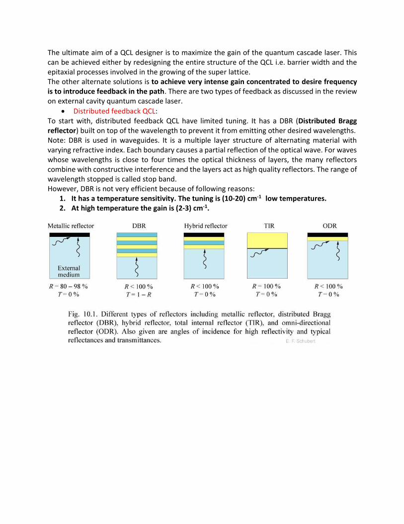
Distributed feedback QCL: To start with, distributed feedback QCL have limited tuning. It has a DBR (Distributed Bragg reflector) built on top of the wavelength to prevent it from emitting other desired wavelengths. Note: DBR is used in waveguides. It is a multiple layer structure of alternating material with varying refractive index. Each boundary causes a partial reflection of the optical wave. For waves whose wavelengths is close to four times the optical thickness of layers, the many reflectors combine with constructive interference and the layers act as high quality reflectors. The range of wavelength stopped is called stop band. However, DBR is not very efficient because of following reasons:

1. It has a temperature sensitivity. The tuning is (10-20) cm-1 low temperatures. 2. At high temperature the gain is (2-3) cm-1.

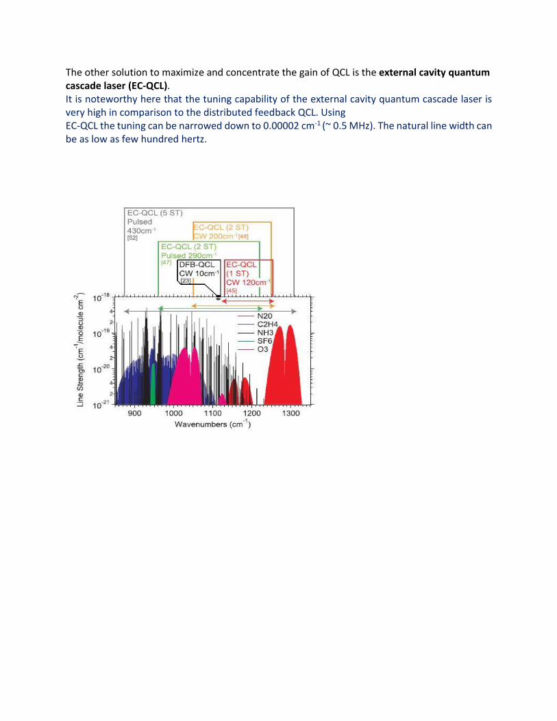
The other solution to maximize and concentrate the gain of QCL is the external cavity quantum cascade laser (EC-QCL). It is noteworthy here that the tuning capability of the external cavity quantum cascade laser is very high in comparison to the distributed feedback QCL. Using EC-QCL the tuning can be narrowed down to 0.00002 cm-1 (~ 0.5 MHz). The natural line width can be as low as few hundred hertz.

The EC-QCL can be understood under the purview of following components: 1. Gain element- The QCL 2. Collimating lenses 3. Grating which is a wavelength filter.

The setup can be explained as under:

There is a chip between the collimating lenses.

The placement of the chip facilitates collection of light from highly divergent QCL.

Collimating light on the right impinges on and selectively reflected by diffraction grating. As grating is rotated light of varying wavelengths are fed back to the QCL chip forcing it to emit narrow line width.

Output is taken from the left.

DIFFRATION GRATING: It is an optical device component with a periodic structure which splits and diffracts light into the several beams. Travelling in different directions. The direction of these beams depends on the spacing and wavelength of the grating acts as dispersive element.

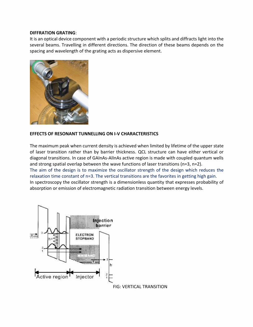
EFFECTS OF RESONANT TUNNELLING ON I-V CHARACTERISTICS The maximum peak when current density is achieved when limited by lifetime of the upper state of laser transition rather than by barrier thickness. QCL structure can have either vertical or diagonal transitions. In case of GAInAs-AlInAs active region is made with coupled quantum wells and strong spatial overlap between the wave functions of laser transitions (n=3, n=2). The aim of the design is to maximize the oscillator strength of the design which reduces the relaxation time constant of n=3. The vertical transitions are the favorites in getting high gain. In spectroscopy the oscillator strength is a dimensionless quantity that expresses probability of absorption or emission of electromagnetic radiation transition between energy levels.

FIG: VERTICAL TRANSITION

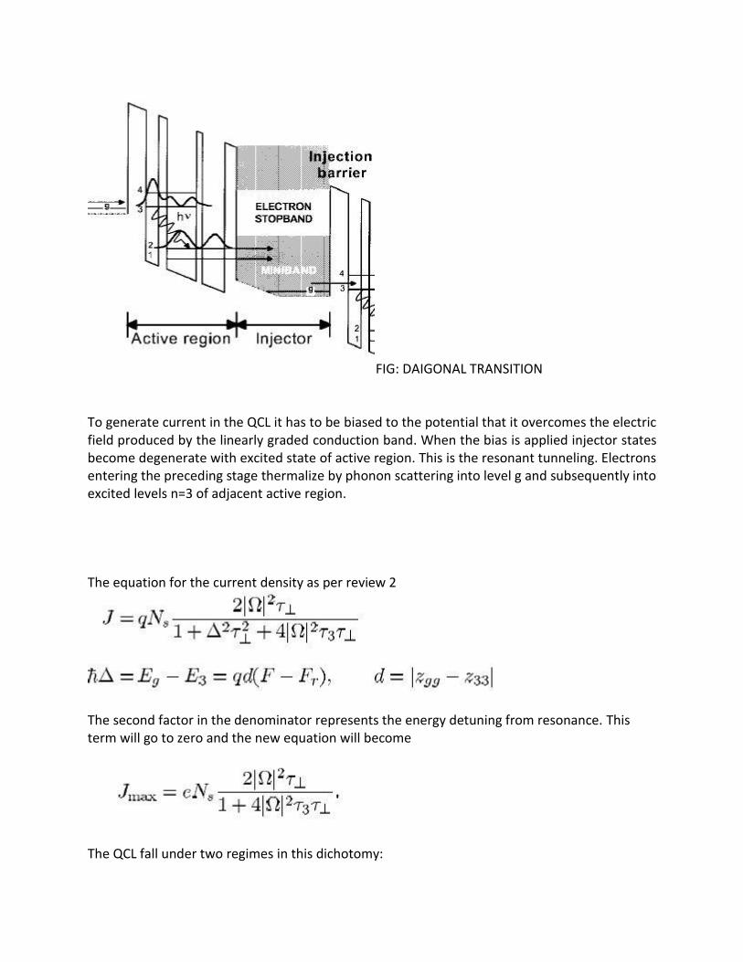
FIG: DAIGONAL TRANSITION To generate current in the QCL it has to be biased to the potential that it overcomes the electric field produced by the linearly graded conduction band. When the bias is applied injector states become degenerate with excited state of active region. This is the resonant tunneling. Electrons entering the preceding stage thermalize by phonon scattering into level g and subsequently into excited levels n=3 of adjacent active region. The equation for the current density as per review 2

The second factor in the denominator represents the energy detuning from resonance. This term will go to zero and the new equation will become

The QCL fall under two regimes in this dichotomy:

Regime 1: The weak injector excited state coupling In this regime we can assume

So the maximum current density is restricted to

Here, we understand that the spatial overlap of quantum waves is less. Regime 2: Strong injector excited state coupling

So the maximum current density is given by

This configuration we want to operate our laser in order to always ensure fast injection into upper state (n=3) without being limited by tunneling rate. So the total current is limited by the lifetime of the excited state.