analysis of the uncertainty of wind power predictions
TRANSCRIPT

Analysis of the Uncertaintyof Wind Power Predictions
Von der Fakultat Mathematik und Naturwissenschaften
der Carl von Ossietzky Universitat Oldenburg
zur Erlangung des Grades eines
Doktors der Naturwissenschaften (Dr. rer. nat.)
angenommene Dissertation.
Matthias Lange
geboren am 21.01.1972
in Wuppertal
Oldenburg (Oldb) 2003

Erstreferent: Prof. Dr. Jurgen Parisi
Korreferent: Prof. Dr. Joachim Peinke
Tag der Disputation: 31.10.2003

Contents
1 Introduction 1
2 Prediction of the power output of wind farms 5
2.1 Motivation for wind power predictions . . . . . . . . . . . . . . . . . . . . . . 5
2.2 Overview of existing systems . . . . . . . . . . . . . . . . . . . . . . . . . . . 7
2.2.1 Physical systems . . . . . . . . . . . . . . . . . . . . . . . . . . . . . 8
2.2.2 Statistical systems . . . . . . . . . . . . . . . . . . . . . . . . . . . . 9
2.2.3 Assessment of forecast errors . . . . . . . . . . . . . . . . . . . . . . 10
2.3 Physical foundations of boundary layer flow . . . . . . . . . . . . . . . . . . . 11
2.3.1 Logarithmic wind profile . . . . . . . . . . . . . . . . . . . . . . . . . 12
2.4 Forecasting method used in this work . . . . . . . . . . . . . . . . . . . . . . 13
3 Data 15
3.1 Numerical weather predictions . . . . . . . . . . . . . . . . . . . . . . . . . . 15
3.2 Measurements . . . . . . . . . . . . . . . . . . . . . . . . . . . . . . . . . . . 16
3.2.1 Wind data and power output of wind farms . . . . . . . . . . . . . . . 16
3.2.2 Atmospheric pressure . . . . . . . . . . . . . . . . . . . . . . . . . . . 18
4 Assessment of the overall prediction uncertainty 19
4.1 Introduction . . . . . . . . . . . . . . . . . . . . . . . . . . . . . . . . . . . . 19
4.2 Basic visual assessment . . . . . . . . . . . . . . . . . . . . . . . . . . . . . . 20
4.3 Distribution of prediction errors . . . . . . . . . . . . . . . . . . . . . . . . . 21
4.4 Statistical error measures . . . . . . . . . . . . . . . . . . . . . . . . . . . . . 26
4.4.1 Decomposition of the root mean square error . . . . . . . . . . . . . . 26
4.4.2 Limits of linear correction schemes . . . . . . . . . . . . . . . . . . . 27

II CONTENTS
4.5 Wind speed prediction error for single sites . . . . . . . . . . . . . . . . . . . 31
4.6 Power prediction error for single sites . . . . . . . . . . . . . . . . . . . . . . 38
4.7 Conclusion . . . . . . . . . . . . . . . . . . . . . . . . . . . . . . . . . . . . 45
5 Smoothing effects in regional power prediction 47
5.1 Introduction . . . . . . . . . . . . . . . . . . . . . . . . . . . . . . . . . . . . 47
5.2 Ensembles of Measurement Sites . . . . . . . . . . . . . . . . . . . . . . . . . 47
5.3 Model ensembles . . . . . . . . . . . . . . . . . . . . . . . . . . . . . . . . . 48
5.4 Conclusion . . . . . . . . . . . . . . . . . . . . . . . . . . . . . . . . . . . . 54
6 Assessment of wind speed dependent prediction error 57
6.1 Idea behind detailed error assessment . . . . . . . . . . . . . . . . . . . . . . 57
6.2 Introduction of conditional probability density functions . . . . . . . . . . . . 58
6.3 Conditional PDF of wind speed data . . . . . . . . . . . . . . . . . . . . . . . 62
6.4 Estimating the distribution of the power prediction error . . . . . . . . . . . . . 67
6.5 Simple modelling of the power prediction error . . . . . . . . . . . . . . . . . 70
6.6 Conclusion . . . . . . . . . . . . . . . . . . . . . . . . . . . . . . . . . . . . 72
7 Relating the forecast error to meteorological situations 75
7.1 Introduction . . . . . . . . . . . . . . . . . . . . . . . . . . . . . . . . . . . . 75
7.2 Methods from synoptic climatology . . . . . . . . . . . . . . . . . . . . . . . 76
7.2.1 Principal component analysis (PCA) . . . . . . . . . . . . . . . . . . . 77
7.2.2 Cluster analysis . . . . . . . . . . . . . . . . . . . . . . . . . . . . . . 79
7.2.3 Daily forecast error of wind speed . . . . . . . . . . . . . . . . . . . . 81
7.2.4 Tests of statistical significance . . . . . . . . . . . . . . . . . . . . . . 82
7.3 Results . . . . . . . . . . . . . . . . . . . . . . . . . . . . . . . . . . . . . . . 83
7.3.1 Extraction of climatological modes . . . . . . . . . . . . . . . . . . . 83
7.3.2 Meteorological situations and their forecast error . . . . . . . . . . . . 88
7.4 Conclusion . . . . . . . . . . . . . . . . . . . . . . . . . . . . . . . . . . . . 104
8 Overall conclusions and outlook 107

CONTENTS III
A Definition of statistical quantities 111
A.1 General statistical quantities . . . . . . . . . . . . . . . . . . . . . . . . . . . 111
A.2 Error measures . . . . . . . . . . . . . . . . . . . . . . . . . . . . . . . . . . 111
B Statistical testing 113
B.1 Theχ2-test . . . . . . . . . . . . . . . . . . . . . . . . . . . . . . . . . . . . 113
B.2 The Lilliefors test . . . . . . . . . . . . . . . . . . . . . . . . . . . . . . . . . 114
B.3 The F-test . . . . . . . . . . . . . . . . . . . . . . . . . . . . . . . . . . . . . 114
B.4 F-test results from chapter 7 . . . . . . . . . . . . . . . . . . . . . . . . . . . 116
Bibliography 116
Acknowledgments 127

IV CONTENTS

Abbreviations V
Abbreviations
ANN Artificial neural networkCET Central European timeCO2 Carbon dioxideDBC Double bias correctionDM Deutschlandmodell by DWDDMI Danish Meteorological InstituteDWD Deutscher Wetterdienst (German Weather Service)EM Europamodell by DWDGM Globalmodell by DWDGMT Greenwich mean timeHIRLAM High resolution local area modelISET Institut fur Solare Energieversorgungstechnik, KasselLM Lokalmodell by DWDLR Linear regressionmeas MeasurementNOx Nitrogen oxideNWP Numerical weather prediction modelPBL Planetary boundary layerPC Principal componentPCA Principal component analysispred PredictionTSO Transmission system operatorUTC Universal time coordinatedWMEP Wissenschaftliches Mess- und Evaluierungsprogramm
(Scientific Measurement and Evaluation Programme)WPPT Wind power prediction tool

VI Mathematical symbols
Mathematical symbols
bias Difference between two mean values (equation A.6)disp Dispersion (equation A.8)ε Difference between prediction and measurementh Height above ground levelκ Von Karman constantP (u) Power curve of wind turbinePmeas Measured power outputPpred Predicted power outputpdf Probability density functionpmsl Atmospheric pressure at mean sea levelpsurf Atmospheric pressure at ground levelr (Cross-) correlationR Dry gas constantrmse Root mean square error (equation A.5)ρ Air densitysdbias Difference between standard deviations (equation A.8)sde Standard deviation of error (equation A.7)T Temperaturetpred Prediction timeτ Turbulent stress tensoru∗ Friction velocity~u = (u, v) Horizontal wind vectorumeas Measured wind speedupred Predicted wind speedz0 Roughness length

1 Introduction
Wind energy is an important cornerstone of a non-polluting and sustainable electricity supply.Due to favourable regulatory frameworks this renewable energy source has experienced atremendous growth in recent years resulting in substantial shares of electricity produced bywind farms in the national energy mix of a number of countries. For example, during the lastfour years (1999 to 2003) the installed wind power capacity in Germany has risen from about4.4 GW to more than 12.8 GW [2] now covering approximately 4.7% of the total electricityconsumption. And this is just the beginning as from a global perspective wind energy has thepotential to provide electric energy on an industrial scale. It is estimated that by the year 2020about 12% of the world’s electricity production can be supplied with wind energy [41].
However, in practice the integration of wind energy into the existing electricity supply system isa real challenge. A number of technical and economical objections against the large-scale util-isation of this renewable energy source have been brought forward, in particular by traditionalenergy suppliers and grid operators. In their view one major disadvantage of wind energy is thatits availability mainly depends on meteorological conditions, hence, the power output of windfarms is determined by the prevailing wind speed and cannot be adjusted as conveniently as theelectricity production of conventional power plants. As it is expensive to level out unforeseenfluctuations in the wind power production, grid operators and energy suppliers, e.g. E.ON [60],point out increasing costs due to wind energy.
The fact that wind energy is not fully compatible to the traditional electricity supply systemcannot be an argument against wind energy but an encouragement to adapt and optimise thesupply system accordingly. This will be unavoidable in the long run as the integration of largeamounts of renewable energies together with the continuing liberalisation of electricity marketsrequire more flexibility in both the production and the purchase of electricity. In particular, inGermany the energy supply system can be changed cost-effectively in order to cope with largeshares of wind energy which has been shown recently by Kramer [28].
Purpose of this work
Wind power prediction systems which improve the technical and economical integration of windenergy into the electricity supply system are already available. They provide the informationhow much wind power can be expected at which point of time in the next few days. Thus,they announce the variations in the electricity production of wind farms in advance and largelyreduce the degree of randomness attributed to wind energy.
This work is concerned with assessing the uncertainty of these wind power predictions. Theuncertainty is the typical range in which deviations between what was predicted and the real sit-uation are likely to occur. The majority of today’s wind power forecasting systems is based on

2 1 Introduction
numerical weather prediction models (NWP) and it is commonly known that NWPs do not pro-vide perfect forecasts. This inconvenient situation has very basic roots as “the laws of physicsdictate that society cannot expect arbitrarily accurate weather and climate forecasts” [49]. Ifforecast errors are in principle unavoidable it is at least good to know as precisely as possiblewhen and how they occur. Hence, in addition to the forecast value itself the prediction systemshould also provide a prediction of the uncertainty of the specific forecast. This is an importantinformation for the users of such systems as it allows them to assess the risk of relying on theforecast.
So far, the forecast uncertainty is mostly estimated by the average error taken over all days ina certain period of time in the past, say a year. This approach disregards that the predictionaccuracy might depend on the complexity of the meteorological situation. But there is reasonto believe that very dynamic weather conditions where low pressure areas with their frontsdominate the flow are harder to predict than rather stable high pressure situations. Thus, itseems appropriate to develop a situation dependent assessment of the forecast error.
In this work the typical errors related to wind power predictions are investigated in greater detailthan before. This includes the assessment of the overall behaviour of deviations between pre-dictions and measurements in terms of statistical distributions, as well as the decomposition ofthe forecast error in amplitude and phase errors. Moreover, the error reduction in the predictionof the combined power output of many wind farms in a region compared to a single wind farmis analysed and the benefits of a regional wind power prediction are quantitatively assessed. Anew situation dependent approach to the prediction error is introduced with the explicit aim toquantify these errors under consideration of the specific forecast situation. Special attentionis paid to two important error sources: the impact of the weather situation on the accuracy ofthe wind speed prediction which is the main input to the power prediction and the role of thenon-linear power curve in amplifying initial errors in the wind speed. The results can be used topredict the specific uncertainty of individual forecasts in an operational wind power predictionsystem.
Structure
This work is organised in the following way.
Chapter 2 explains why wind power predictions are useful and how they are made. The mo-tivation and the benefits of wind power predictions are described in detail. An overview of aselection of existing wind power prediction systems is given to illustrate differences and sim-ilarities in the various concepts. Moreover, the relevant physical relations that are used in thiswork are derived from basic concepts of boundary layer meteorology and the applied forecast-ing method to translate predicted wind speed into power output is described.
The data basis used in the investigations of this work consists of measurements on the one handand numerical predictions on the other hand. The origin and pre-processing of the two types ofdata are explained in chapter 3.
The overall accuracy of the wind speed and power predictions for single wind farms is investi-gated in chapter 4. Suitable error measures are introduced that allow to distinguish amplitude

3
from phase errors. The main statistical features in terms of the average forecast errors and theirprobability distributions are analysed for both the wind speed and power output.
As for practical purposes the combined power output of many spatially dispersed wind farms isof greater interest than that of a single one chapter 5 deals with regional smoothing effects andis an important step beyond the single site perspective.
Chapter 6 introduces the idea of a situation dependent assessment of the prediction error. In afirst step the wind speed is investigated in detail, in particular the question whether the forecastaccuracy depends on the magnitude of the wind speed. Moreover, the relationship between theprobability distributions of the forecast error of wind speed and power output is derived. Inaddition, the important role of the non-linear power curve in amplifying initial errors in thewind speed forecast according to its local derivative is quantified and a simple model to predictthe specific forecast uncertainty is developed.
Chapter 7 continues the situation dependent assessment of the forecast error and deals with thequantitative relation between the type of weather conditions and the corresponding predictionaccuracy. Methods from synoptic climatology are used to automatically classify weather situa-tions based on a suitable set of meteorological variables. The typical prediction errors in eachweather class are determined in order to find out whether dynamic low pressure situations arereally harder to predict than stable high pressure types.
Finally, chapter 8 contains an overall summary with conclusions and an outlook.

4 1 Introduction

2 Prediction of the power output of wind farms
Abstract
This chapter motivates why power predictions improve the technical and economical integration of wind
energy into the electricity supply system. An overview of existing wind power prediction systems is
given and the different approaches behind them are briefly explained. In addition, the relevant physical
relations that are used in this work are derived from basic concepts of boundary layer meteorology and
the applied forecasting method to translate predicted wind speed into power output is described.
2.1 Motivation for wind power predictions
In contrast to conventional power plants the electricity production of wind farms almost entirelydepends on meteorological conditions, particularly on the magnitude of the wind speed, whichcannot directly be influenced by human intervention. Though this is a rather trivial fact it makesa profound difference, technically as well as economically, in the way large amounts of wind en-ergy can be integrated into electrical grids compared to the conventional sources. The so-calledfluctuating or intermittent nature of the wind power production due to unforeseen variations ofthe wind conditions means a new challenge for the players on the production and distributionside of the electricity supply system and is often used as an argument against the utilisation ofwind power. Hence, the reputation and the value of wind energy would considerably increaseif fluctuations in the production of wind power were known in advance. To provide this infor-mation is exactly the purpose of wind power prediction systems. They are designed to producea reliable forecast of the power output of wind farms in the near future such that their expectedcontribution can be efficiently integrated into the overall electricity supply.
In order to assess the benefits of wind power predictions in more detail and derive the boundaryconditions for their operational use some aspects of the electricity supply system have to befurther explained.
A secure electricity supply requires that at each point of time the electricity production matchesthe demand as exactly as possible. It is the task of the transmission system operator (TSO) tocarefully keep this balance. The load, i.e. the total consumption of electric power of householdsand industry, and its variations over the day are rather well known from experience and areexpressed by so-called load profiles. These daily load patterns are used to estimate the electricitydemand of the next day with a relatively high accuracy.
In a world without wind energy the load profiles are sufficient for the TSO to work out a ratherprecise plan how to satisfy the demand on a day-ahead basis. In a liberalised market environ-ment the TSO basically has two options: produce electricity using its own power plants or buyelectricity on the market. In the case of own production a schedule for the conventional power

6 2 Prediction of the power output of wind farms
plants is made today that defines the number and type of power plants to be in operation tomor-row. Hence, the time horizon for the scheduling is about 48 hours. This time-table considersthe special characteristics of the different kinds of power plants such as time constants to comeinto operation or fuel costs. If electricity is bought or sold on a day-to-day basis on the energymarket bids also have to be made about 48 hours in advance. How the two options are combineddepends on technical as well as economical considerations, e.g. described in [51].
However, large shares of wind energy spoil this nicely established scheme to a certain degree,especially, if wind power is unexpectedly fed into the system. From the point of view of theTSO wind power acts as a negative load because the demand of electricity that has to be met byconventional power plants is reduced by the proportion of wind power available in the grid. Thiscan be quite substantial in areas with high grid penetration of wind energy where the installedwind power is of the order of magnitude of the minimum load which is, e.g., the case for certainareas in northern Germany or Denmark.
In Germany TSOs mainly deal with this situation by using additional control power [60, 10].Control power is generally applied to compensate for sudden deviations between load and pro-duction and can also be used to balance the fluctuating behaviour of wind power in the electricalgrid. Keeping control power aims at being prepared for surprising situations, e.g. due to an un-expected drop in the power output of wind farms which can be rather dramatic if many windfarms in a supply area switch themselves off for security reasons during a storm and the produc-tion decreases considerably. As surprises are not the kind of thing that are highly appreciatedby TSOs the amount of control power related to wind energy is quite substantial and, therefore,expensive. A fact that is constantly pointed out by the TSOs, e.g.[60]. Moreover, control powerdiminishes the environmental benefits of wind energy as it is technically realised by either mak-ing power plants operate with a reduced degree of efficiency or activate additional fossil fueldriven plants [36, 10]. Hence, the energy corresponding to control power that is additionallyused to compensate for fluctuations in wind power has to be subtracted from the energy fed intothe grid by wind farms which, unfortunately, reduces the amount of avoided CO2 emissions.
These considerations show that a sufficiently accurate prediction of the power output of windfarms with a time horizon of at least 48 hours is necessary for TSOs to efficiently integratesubstantial shares of wind power into the existing electricity supply system. Such a predictionprovides the decisive information concerning the availability of wind power over the next oneto two days. Thus, wind power can be considered in the scheduling schemes of conventionalpower plants as well as in decisions to purchase energy on the market.
The benefits are obvious because the amount of control power can be decreased if the predictionis reliable enough. Dany [10] found a quasi-linear relation between the forecast error and theneed for control power caused by wind energy, thus, each percent improved prediction accuracyleads to a reduction of control power by the same proportion. The operational use of a reliablewind power prediction system enables TSOs not only to save money by using less control powerbut, in addition, the information how much wind power will be available allows to trade windpower on the electricity market. It has already been illustrated for the Scandinavian situation byMordhorst [43] that wind energy can be profitably traded on a liberalised market, in particular,on the spot market, and Holttinen et al. [22] found that today’s wind power prediction systems

2.2 Overview of existing systems 7
can already improve the income achieved by selling wind power under short-term market con-ditions. Hence, wind power forecasts increase the economic value of wind energy and help tomake this renewable energy source competitive with conventional ones. In addition, the envi-ronmental advantage of wind energy is further increased as unnecessary CO2 emissions due tocontrol power are reduced.
2.2 Overview of existing systems
In recent years a number of systems to predict the power output of wind farms have been devel-oped. As discussed above the required time horizon is given by the scheduling scheme of theconventional power plants and the bidding conditions on electricity markets which are typicallyof the order of one to two days ahead. Hence, prediction systems are required to provide theexpected power output from 6 to at least 48 hours, preferably in an hourly resolution.
Note that the time horizon is very important as from a modelling point of view there is a funda-mental difference between so-called short-term predictions on time scales of a few days that areconsidered here and very short-term predictions in the range of 0 to 3 hours. While the longertime period is rather well described by numerical weather prediction systems which explicitlymodel the dynamics of the atmosphere the very short range is typically dominated by persist-ing meteorological conditions where purely statistical approaches lead to better forecast results,e.g.[7, 44].
Most of the existing power prediction systems are based on the results of numerical weather pre-diction systems (NWP). Hence, all the information about the future, in particular the expectedevolution of the wind field, is provided by the NWP. These systems simulate the developmentof the atmosphere by numerically integrating the non-linear equations of motions starting fromthe current atmospheric state. The accuracy of the numerical predictions over the desired timehorizon is typically far better than any type of statistical or climatological approach.
The wind vector, i.e. wind speed and wind direction, is, of course, the most important variablein terms of wind power prediction. It is the task of the wind power prediction system to convertthis “raw information” typically given with a rather coarse spatial resolution by the NWP intoan adequate prediction of the power output of a wind farm. There are basically two approachesto transform the wind prediction into a power prediction. On the one hand physical systemscarry out the necessary refinement of the NWP wind to the on-site conditions by methods thatare based on the physics of the lower atmospheric boundary layer. Using parametrisations ofthe wind profile or flow simulations the wind speed at the hub height of the wind turbines iscalculated. This wind speed is then plugged into the corresponding power curve to determinethe power output. On the other hand statistical systems in one or the other way “learn” therelation between wind speed prediction and measured power output and generally do not usea pre-defined power curve. Hence, in contrast to physical systems the statistical ones needtraining input from measured data.

8 2 Prediction of the power output of wind farms
2.2.1 Physical systems
One of the first physical power prediction systems with a prediction horizon up to 72 hours wasdeveloped by Landberg [29, 30] at the National Laboratory in Risø in 1993. The procedure isbased on a local refinement of the wind speed prediction of the NWPHIRLAM [53] operatedby the Danish Meteorological Institute. The refinement method to adapt the NWP output tothe local conditions at the site was derived from techniques that had been used before for windpotential assessment in the framework of the European Wind Atlas [62]. Local surface rough-ness, orography describing the hilliness of the terrain, obstacles, and thermal stratification ofthe atmosphere are taken into consideration leading to forecast results that were significantlybetter than persistence, i.e. the assumption that the current value is also valid in the future. Theprediction system has been commercialised under the namePrediktor for operational use.
eWindhas been introduced by Bailey et al. [3] and is a prediction system that is physical interms of local refinement of the wind conditions but statistical in terms of determining thepower output. It uses a meso-scale atmospheric model (MASS) that is driven by a regionalNWP with a coarser resolution. This process is called nesting where the idea is here to usea high-resolution model only in areas of special interest, e.g. at the location of a wind farmto cover atmospheric effects on a smaller scale that cannot be resolved by the coarser model.Hence,eWindactually simulates the local flow instead of using a parametrisation of the windprofile. However, adaptive statistical methods which require on-site measurement data are usedin the last step to translate wind speed into power and to correct for systematic errors in theprediction.
Instead of using the NWP wind speed forecast as given input and modify it afterwards for windpower applications Jørgensen et al.[25] follow a more general approach by implementing windpower forecasts directly into the large-scale weather prediction systemHIRLAM. Again nestingis used to increase the spatial resolution of the NWP in order to optimise the system with regardto accurate wind speed forecasts. As it is directly related to the NWP the power predictionsystem can take full advantage of the complete set of meteorological variables provided by theweather model in its internal temporal resolution which is typically much higher than the usualtime steps of one hour provided to customers.
The power prediction systemPrevientohas been developed at the University of Oldenburg [5,42] and is in operational use in Germany. It is based on the same principle asPrediktor in termsof refining the prediction of wind speed and wind direction taken from the NWP as illustrated infigure 2.1. The local conditions are derived by considering the effects of the direction dependentsurface roughness, orographic effects and, in particular, atmospheric stability [15, 14] on thewind profile. Moreover, the shadowing effects occurring in wind farms are taken into account.If measurement data from the wind farms are available a systematic statistical correction offorecast errors is applied. As in practice the combined power output of many spatially dispersedwind farms in a region is of greater interest than that of a single wind farm,Previentocontains anadvanced up-scaling algorithm that determines the expected power output of all wind farms ina certain area based on a number of representative sites selected in an appropriate manner [17].In addition to the power prediction itselfPrevientoalso provides an estimate of the uncertaintyof the specific forecast value [18] to allow users an assessment of the risk of relying on the

2.2 Overview of existing systems 9
prediction. Regarding the regional up-scaling and the uncertainty estimates a part of the resultsof this work have been implemented intoPrevientoand will be described in more detail inchapters 5 and 7. For the investigations in this workPrevientowill only be used in a very basicmode as described in section 2.4.
Spatial RefinementLocal Roughness, Orography,
Atmospheric Stability
Wind Vector, Atmospheric Pressure
Power Curve
Wind Turbine
Wind Farm Effects
Prediction of Power Output
Numerical Weather Prediction
Transformation to Hub Height
Systematic Error Correction
Figure 2.1: In full mode the prediction systemPrevientocarries out a spatial refinement ofthe numerical weather prediction. It takes local surface roughness at the site, orography andatmospheric stability into account leading to a local prediction of wind conditions and windpower. In order to focus on the major effects of the underlying NWP prediction and the influenceof the power curve, in particular, the refinement procedure ofPrevientohas not been used inthis work and the steps in the dashed boxes have been omitted.
2.2.2 Statistical systems
WPPT is a statistical system that has been used operationally in Denmark for many years. Itwas developed by Nielsen and Madsen [47, 48] at the Danish Technical University. ThoughWPPT contains some deterministic elements such as the diurnal cycle it basically learns therelation between predicted wind speed and measured power output with no local refinementinvolved. Mathematically, the system is based on time-varying coefficient functions which are

10 2 Prediction of the power output of wind farms
continuously re-calculated using NWP input on the one hand and measurement data on theother hand. This has the advantage that the parameters are automatically adapted to long-termchanges in the conditions, e.g. variations in roughness due to seasonal effects or model changesin the NWP.
For use in complex terrain in SpainWPPT has been modified by Marti et al. [40] using theSpanish version ofHIRLAM as input. However, as both the type of terrain and the climate ofthe Iberian peninsula are rather challenging, a new model chain, calledLocalPred[39], is beingdeveloped that intends to combine statistical time series forecasting and high resolution physicalmodelling based on meso-scale models.
A system for on-line monitoring and prediction of wind power that is in operational use atseveral German TSOs comes from the Institut fur Solare Energieversorgungstechnik (ISET) inKassel and has recently been namedWPMS[11, 12]. The system uses NWP output of severalmeteorological variables where the predicted wind speed is refined to local conditions in termsof a look-up table by applying a meso-scale atmospheric model. To relate the predicted variablesto measured power output of a certain set of wind farms artificial neural networks (ANN) areused.
It has to be said that the distinctions between physical and statistical systems are fading as ad-vanced approaches incorporate the best out of both categories. Quite naturally, physical methodssuch as meso-scale models are used for local refinement of coarse NWP output to the on-siteflow conditions dominated by rather well-known deterministic effects while statistical methodsare beneficially applied to correct for systematic errors and to aquire empirical knowledge onsite-dependent power curves.
This overview of wind power prediction systems does not claim to be complete as more andmore models are under development at many research institutes and companies all over theworld. There has been a tremendous increase in the number of systems over the last few yearsunderlining the importance of reliable forecasting tools to efficiently integrate wind power intothe electricity supply system, in particular in view of the very ambitious plans for offshoreinstallations of wind farms in many European countries.
2.2.3 Assessment of forecast errors
So far, the assessment of the uncertainties of these wind power prediction systems has mainlybeen restricted to the overall accuracy, i.e. the average forecast error over all days and weathersituations in a certain period of time, preferably a year. Hence, in most cases the individualforecast situation is not taken into account. However, an early investigation to provide specificconfidence intervals for individual power predictions was carried out by Luig et al. [38]. Theyused so-called beta-distributions to approximate the conditional probability density functions ofthe power prediction error. Hence, the magnitude of the prediction value determined the uncer-tainty range. A different approach has been pursued by Landberg et al.[31] and, recently, Pinsonand Kariniotakis [50] who used a kind of ensemble prediction (explained in more detail in chap-ter 7). They estimated the uncertainty of the forecast by evaluating the spread in the values ofthe wind speed prediction valid for the same point of time in the future but from succeedingforecast runs. Hence, the inherent properties of the NWP were used to assess the predictability

2.3 Physical foundations of boundary layer flow 11
of the prevailing forecast situation. In contrast to these previous approaches this work focuseson the relation between the actual weather situation classified by a suitable set of meteorologicalvariables and the corresponding prediction error of the NWP. This has the advantage that theoccurrence of forecast errors can easier be understood in terms of meteorological phenomena.
2.3 Physical foundations of boundary layer flow
The physics of the atmosphere is rather complex as it is a non-linear system with an infinitenumber of degrees of freedom but the dynamics can in principle be described by equations ofmotion that are derived from the principles of conservation of mass, momentum and energy.Though these equations can be found in standard meteorological textbooks, e.g. [57, 52], ap-proximate analytical as well as numerical solutions for non-trivial states of the atmosphere canin most cases only be obtained by simplifying assumptions.
In order to separate different flow regimes the atmosphere is divided into several horizontallayers. These layers are defined by the dominating physical effects that influence the dynamics.In the context of wind energy applications the troposphere which spans the first five to tenkilometres above the ground has to be considered as it contains the relevant wind field regimesas illustrated in figure 2.2.
plan
etar
y bo
unda
ry la
yer
surf
ace
laye
r
trop
oshe
reclouds
geostrophic wind
logarithmic wind profile
0.01
0.1
1
10
100
1000
10000
0 1 2 3 4 5 6 7 9 10
wind speed [m/s]
8
heig
ht [m
]
Figure 2.2: Schematic illustration of the horizontal layers in the troposphere which comprisesthe lower part of the atmosphere that is important for wind energy. In the top layer aboveapproximately 1 km there is little influence of the ground and the wind is geostrophic drivingthe flow in the lower layers. The wind field in the surface layer (up to about 100 m) is mainlydominated by friction exerted by the ground and turbulent mixing. Under certain assumptionsa logarithmic profile can be derived for the wind speed.

12 2 Prediction of the power output of wind farms
Heights above approximately 1 km are the domain of large-scale synoptic pressure systems.Their wind field is largely dominated by the Coriolis force, caused by the rotation of the earth,as well as the horizontal gradients of pressure and temperature. As the influence of the ground israther weak Coriolis force and pressure gradient force can typically be considered as balancedleading to the geostrophic wind that blows parallel to the isobars.
This geostrophic wind field is regarded as the main driving force of the flow in the underlying at-mospheric layer denoted as planetary boundary layer (PBL). The wind in the PBL is dominatedby the influence of the the friction exerted by the earth’s surface. Typically, the flow near thesurface is turbulent which provides a very effective coupling mechanism between wind speedsat different heights leading, in particular, to vertical transport of horizontal momentum that isdirected towards the ground where the wind speed has to vanish. This momentum flux based onturbulent mixing is by far larger than it would be based on molecular viscosity alone such thatthe change of the surface wind with height strongly depends on the degree of turbulence in theatmosphere.
Two different mechanisms of turbulence generation have to be distinguished. Mechanical tur-bulence induced by wind shear on the one hand and convective turbulence due to buoyancy onthe other hand. Buoyancy is mainly caused by heating of the atmosphere from below, e.g.due tothe irradiation of the sun. The type and degree of turbulence generation influences the stabilityproperties of the atmosphere and, hence, the shape of the wind profile.
2.3.1 Logarithmic wind profile
In order to describe the variations of wind speed at heights up to approximately 100 m over ahomogeneous surface the logarithmic profile is used. It can be derived under the assumptionsthat the atmosphere is neutral, i.e. mechanical turbulence dominates, that the pressure gradientas well as the Coriolis force can be ignored, and that the turbulent momentum flux can beregarded as constant with height. The procedure to derive the logarithmic profile shown herefollows Arya [1].
The vertical flux of horizontal momentum can be summarised by the turbulent stress ten-sor τ that implicitly contains the information concerning both the driving force given by thegeostrophic wind and the coupling of the wind speeds at different heights.τ is assumed tobe constant in the surface layer. If normalised to the air densityρ the momentum flux canconveniently be expressed by the so-called friction velocity,
u∗ :=
√τ
ρ, (2.1)
being the characteristic velocity scale of the flow in the surface layer.
From dimensional analysis it follows that the vertical wind speed gradientdu/dz has to scalewith the characteristic velocityu∗ and the heightz which is the typical length, hence,
du
dz=
1
κ
u∗z
(2.2)
whereκ is the von Karman constant which can only be found empirically and has a value ofabout 0.40.

2.4 Forecasting method used in this work 13
Relation (2.2) can also be derived from the concepts of eddy-viscosity and the mixing lengthhypothesis [1]. But there is still no rigorous way to extract this relation from the basic equationsof motion.
The integration of equation (2.2) leads to the well-known logarithmic wind profile
u(z) =u∗κ
ln
(z
z0
). (2.3)
The integration constantz0 is called roughness length as it is related to the surface roughnessand varies over several orders of magnitude depending on the terrain type.
Note that the logarithmic profile does not describe the instantaneous wind speed at any timebut a time averaged wind profile not resolving the details of turbulent fluctuations in the flow.Hence, in order to compare equation (2.3) to measurements the data have to be averaged oversuitable time intervals of the order of 10 min. The log-profile has been confirmed by manyobservations of wind speeds in near-neutral conditions.
For the investigations in this worku∗ does not have to be determined because equation (2.3) isonly used to translate the wind speed from one heighth1 to a different heighth2. Forming theratiou(h2)/u(h1) and solving foru(h2) gives
u(h2) = u(h1)ln
(h2
z0
)
ln(
h1
z0
) . (2.4)
For a further discussion of corrections to the logarithmic profile in the context of wind powerapplications onshore and offshore see [14, 59, 32].
2.4 Forecasting method used in this work
The method used in this work to translate the predicted wind speed into a prediction of thepower output of a wind turbine or wind farm forecasting is very elementary. Only the twoessential steps are performed: the predicted wind speed is transformed to the hub height ofthe wind turbine using equation (2.4) together with the roughness lengthz0 of the NWP. It isthen plugged into the certified power curve of the wind turbine which translates wind speedinto power output. Hence, virtually no local refinement is applied. This is done in order toconcentrate on the major effects, namely the predicted wind speed as it is given by the NWPand the impact of the non-linear power curve. A stability correction would be desirable butdetailed information about atmospheric stratification is not available in the data set.
The typical power curve,P (u), of a wind turbine is shown in figure 2.3. One important char-acteristic is the non-linear shape withP (u) being proportional tou3 for small wind speedsu, arather steep slope for medium wind speeds and the saturation for large wind speeds. In addition,there is a finite cut-in speed at about 3 to 4 m/s, i.e. the wind speed has to be larger than a criticalvalue to get the wind turbine into operation.
It can easily be seen that the characteristic shape of the power curve will influence the forecasterror of the power prediction. Imagine the original wind speed prediction provides a value

14 2 Prediction of the power output of wind farms
0
20
40
60
80
100
120
0 2 4 6 8 10 12 14 16
Pow
er o
utpu
t [%
/Pin
st]
windspeed [m/s]
large deviation
small deviation
Figure 2.3: Power curve of a typical wind turbine. Above the cut-in speed of about 4 m/sthe power production increases rather rapidly. At wind speeds around 12 m/s and higher thewind turbine keeps the power output at a rather constant level because a further increase of therotor speed would lead to too high mechanical loads on the structure. For security reasons themachine shuts down for wind speeds beyond typically 20 m/s. The power curve is non-linearand, hence, the amplification of errors in the wind speed prediction due to the local derivativeof the power curve depends on the wind speed. In intervals with a steep slope small errors inthe speed result in large deviations in the power output. Whereas for very small wind speedsbelow the cut-in speed or very high speeds above 12 m/s the error in the wind speed predictionis dampened by the small slope.
that has a small deviation from the measured “real” value of the wind speed. In the steep partof the power curve this small difference in the wind speed is transferred to a relatively largerdifference between the corresponding predicted and measured power outputs. In contrast to this,if a small deviation in the wind speed prediction occurs in the flat part of the power curve wherethe derivative nearly vanishes, the error in the power prediction is relatively small. Hence, thepower curve amplifies or dampens initial deviations in the wind speed prediction according toits local derivative.
The complete scheme of the prediction systemPrevientohas been introduced in section 2.2.1.ThoughPrevientois used in principle it is run in a base mode. The parts that have been omittedin the investigations in this work are indicated by dashed boxes in figure 2.1. The details of therefinement models have been thoroughly investigated by Monnich [42] and Focken [14, 15].They found that mainly the consideration of orographic effects and thermal stratification of theatmosphere can lead to major improvements of the prediction accuracy compared to the directuse of the NWP input while including the local surface roughness does not necessarily reducethe forecast error. In terms of the power prediction the relative improvement that can typicallybe achieved by including stability corrections into the logarithmic profile is about 5% [14].

3 Data
The data that are used in the investigations of the next chapters fall in two categories: predictionand measurement. Though it is quite straightforward to verify predictions at a certain site withthe corresponding measured data, the origin and the way in which both data types are calculatedor collected, respectively, deserve some discussion.
Predictions, on the one hand, are the result of a numerical integration of the equations of motionsof the atmosphere discretised on a computational grid with a rather coarse resolution of theorder of 10 by 10 km2. Hence, the predicted variables represent a spatial average over the gridcell rather than a point value. This has to be kept in mind, in particular, with respect to thewind vector which is sensitive to the local conditions while scalar quantities are not that muchaffected.
To evaluate the accuracy of these predictions it is desirable to compare them to the “real” valuesof the meteorological variables. As usual in physics measurements which are not arbitrarilyaccurate are used to approximately assess reality in this respect. In contrast to the predictions,the measurements are taken at points. For example, the cup anemometers that are usually usedto measure wind speeds have a typical diameter of the order of 0.1 m which, together with theirrather short response time due to inertia, enables a very localised measurement in space andtime.
The common approach to compare both data types at a given location is by time-averaging themeasured time series over a suitable time interval. This primarily aims at eliminating the highfrequent fluctuations due to turbulence on the time scale below 10 min as these small scalescannot at all be resolved by the NWP. Experience shows that a reasonable averaging periodis around half an hour to one hour. This time interval captures the temporal variations of themeteorological parameters at a synoptic scale and is, therefore, believed to correspond to thespatial average provided by the prediction values of the NWP.
3.1 Numerical weather predictions
All prediction data used in this work are provided by the NWP of the German weather ser-vice (DWD). The investigations are based on the results of the “Deutschlandmodell” (DM)version 4 [54] which has a spatial resolution of 14× 14 km2 horizontally. In the vertical dimen-sion the model comprises 30 levels extending up to 25 km height where the two lowest of theselevels are approximately at 34 m and 111 m height. The domain of the DM completely coversCentral Europe and the British Isles. The boundary values of the DM are set by the Europeanmodel EM with a resolution of about 55× 55 km2 which is itself nested into the global modelGM which spans the whole earth. The DM data are received as points on the computationalgrid. To determine the forecast values at arbitrary locations the values at the four nearest gridpoints are interpolated using inverse distance weights.

16 3 Data
From the two main runs of the DM started every day at 00 UTC (1 h CET) and 12 UTC (13 hCET) only data from the earlier run are available at the prediction times +6, +12, +18, +24, +36and +48 h. These times are counted relative to the starting time, 00 UTC, of the forecast runand, hence, directly correspond to the actual time of the day in UTC.
Previous investigations, e.g. [42], showed that in the context of wind power predictions the useof the predicted wind vector from the diagnostic level at 10 m height leads to better results thaninput from the genuine model levels at 33 m or 110 m. This is surprising at first glance becausethe wind field at a diagnostic level is derived from higher levels by a parametrisation of the windprofile rather than a solution of the equations of motion. However, this parametrisation includesthe logarithmic wind profile and stability corrections which seems to lead to a more suitableinput for the procedures that are used afterwards to translate wind speed to the power output ofwind farms.
The DM predictions used here are from the years 1996, 1997 and 1999 where the focus is on1996 due to the highest data availability in this year. The data of the year 1999 differs from theother years as the predictions are provided as point predictions that already interpolated to thelocation of the wind farm by the weather service. Moreover, the wind speed prediction is givenin a resolution of 1 knot (approximately 0.5 m/s) compared to 0.1 m/s in 1996/97.
The DWD currently operates the “Lokalmodell” (LM) which replaced the DM in November1999. The new model LM has a higher spatial resolution of 7× 7 km2. Moreover, compared toDM it is based on a different set of equations of motions and is, in particular, non-hydrostatic.But these changes do not seem to lead to a dramatically different performance of the LM withregard to the wind speed prediction as first investigations suggest [59].
3.2 Measurements
3.2.1 Wind data and power output of wind farms
In the framework of the WMEP programme (Scientific Measurement and Evaluation Pro-gramme) funded by the German federal government the electrical power output of wind turbineshas been recorded on a regular basis since 1990. In addition, wind speed and wind direction aremeasured at either 10 m or 30 m height on a nearby met mast. The time series are sampled in5 min intervals which is more than sufficient for the investigations in this work. As discussedabove the time series of all involved quantities are averaged over one hour to make them com-parable to the predictions of the NWP. This means that the power output is effectively integratedover one hour such that it corresponds to the amount of electrical energy produced in this timeperiod. Moreover, the averaged values of wind speed and direction are also used to assess thelocal meteorological conditions (chapter 7).
In the remaining chapters measurements from about 30 WMEP sites are used. The map infigure 3.1 shows the locations of the sites, mainly from the northern half of Germany, consideredin this work. As availability and quality of the data varies significantly from site to site andamong different years most of the following investigations will be restricted to a subset of thetotal set of stations.

3.2 Measurements 17
Figure 3.1: Set of 30 WMEP sites in Germany with measurements of wind speed, wind directionand power output of wind turbines that are used to verify the predictions and to assess thelocal meteorological conditions. The underlined stations are used for detailed investigations inchapters 4 and 7.

18 3 Data
3.2.2 Atmospheric pressure
Measurements of atmospheric pressure will be considered in the assessment of the meteorolog-ical conditions at a site. However, as the WMEP sites are not equipped with readings of surfacepressure the measurements from the nearest synoptic station of the German Weather Service(DWD) are used. The distance between the sites and the synoptic stations are in the range from5 to 30 km but this is regarded as uncritical because horizontal gradients of the pressure varyonly little on this scale. In contrast to the WMEP data the pressure time series are recorded onan hourly basis which is appropriate to account for changes on a synoptic scale.
To normalise all sites to a common pressure level the surface pressure,psurface, at ground levelis corrected to the pressure at mean sea level (pmsl) using the barometric height formula:
pmsl = psurface eghRT (3.1)
whereg is the gravitational constant,h the height of the synoptic station above mean sea level,R the dry gas constant andT is the surface temperature which is also measured at the synopticstation.

4 Assessment of the overall prediction uncertainty
Abstract
This chapter supplies an overview over different aspects of the prediction accuracy. The accuracy ofthe predictions is assessed by comparing predicted wind speeds and power outputs with correspondingmeasurements from a selection of six out of 30 sites in Germany. Starting from a visual inspection of thetime series the statistical behaviour of the forecast error is investigated showing strong evidence that thedifferences between predicted and measured wind speed are normally distributed at most sites while thedistribution of the power differences is far from Gaussian. To quantitatively assess the average forecasterror the root mean square error (rmse) is decomposed into different parts which allow to distinguishamplitude errors from phase errors. The analysis shows that amplitude errors can mainly be attributed tolocal properties at individual sites while phase errors affect all sites in a similar way. The relative rmseof the power prediction is typically by a factor 2 to 2.5 larger than that of the wind speed prediction. Itturns out that this is mainly caused by the increased relative amplitude variations of the power time seriescompared to the wind time series due to the non-linear power curve. In addition, the cross-correlation isvirtually not affected by transforming wind speed predictions to power output predictions. Hence, phaseerrors of the wind speed prediction are directly transfered to the power prediction. Moreover, the inves-tigation indicates that there is little space for correction schemes that are based on linear transformationsof the complete time series to substantially improve the prediction accuracy.
4.1 Introduction
Predictions of the future development of meteorological variables are not perfect which is con-tinuously confirmed by every-day experience as well as scientific investigations. Hence, inorder to use and to improve forecasting systems the quality of the predictions has to be eval-uated where “quality” refers to a judgement of how good or bad the prediction is. For thispurpose the predicted values are typically compared with the corresponding measurements. Inthe case of continuous variables such as wind speed the easiest way to get an idea of the qualityof the forecast is by plotting the two time series and visually assess the deviations between themwhich is used in this chapter to illustrate typical errors that can occur.
In general, the quantitative assessment of the relationship between forecast and prediction in-volves the use of standard statistical methods that will be referred to as error measures. Theseerror measures are based on calculating a suitable average over the deviations between predictedand measured values over a certain time period either by using the straightforward differencebetween the two or by taking the squared difference to eliminate the signs. Hence, in this workthe expression “error” refers to the numerical value found by applying one of the error measuresto the predicted and measured time series. However, note that the difference between predictionand measurement is denoted as pointwise error.

20 4 Assessment of the overall prediction uncertainty
Of course, using the error measures requires that the data has already been recorded, i.e. theerror is always a historical value representing the forecast quality of the past. The uncertainty,on the other hand, is understood as the expected error of future predictions which is a prioriunknown. Under the assumption that the statistics of the errors is stationary the historical erroris used as an estimate of the uncertainty.
In order to interpret the error as well as the uncertainty as confidence intervals, i.e. as a certainrange around the predicted value in which the measured value lies with a well-defined probabil-ity, the underlying distribution of the differences between prediction and measurement has to beknown. Therefore, the statistical distributions of the pointwise prediction errors are investigatedfor the wind speed and the power prediction.
4.2 Basic visual assessment
The 6 to 48 h predictions are calculated using equation (2.4) based on the 10 m wind speedprediction of the daily 00 UTC run of the “Deutschlandmodell” (DM) (see section 3.1). Agraphical representation of the predicted and measured data conveys a first impression of theforecast accuracy. In figures 4.1 and 4.2 the time series of the power prediction of a singlewind turbine in the North German coastal region over an interval of six days are compared tothe corresponding WMEP measurement data in an hourly resolution. The overall agreementbetween the two time series is rather good in the period of time shown in figure 4.1 while thesample in figure 4.2 illustrates a poor forecast accuracy.
0
0.2
0.4
0.6
0.8
1
322 323 324 325 326 327 328
pow
er [
% in
stal
led
pow
er]
day of year [d]
measurementprediction
Figure 4.1: Comparison of the time series of measured and predicted (6 to 24 h) power outputnormalised to rated power at one site. The agreement between the two time series is rathergood over the shown period. In particular, the increase in wind speeds on days 323 and 325 iscorrectly predicted. However, the amplitudes, especially on day 326, do not completely fit.

4.3 Distribution of prediction errors 21
0
0.2
0.4
0.6
0.8
1
252 253 254 255 256 257 258
pow
er [
% in
stal
led
pow
er]
day of year [d]
measurementprediction
Figure 4.2: Same as figure 4.1 but for a period of time with a rather poor agreement. Twocharacteristic errors can be observed: On day 254 a typical amplitude error occurs where theprediction is in phase with the measurement but strongly overestimates the real situation. Incontrast to this, on day 257 the amplitude of the prediction is right but the maximum wind speedappeared several hours earlier and decayed faster than predicted. Hence, this situation is anexample for a phase error.
This example highlights two characteristic sources of error occurring in the forecasting busi-ness: deviations in amplitude, i.e. overestimation or underestimation by the forecast but witha correct temporal evolution (as on day 254 in figure 4.2), and phase errors, i.e. the forecastwould match the real situation if it was not shifted in time (day 257). The following statisticalinvestigation has to account for these effects and must, therefore, be based on error measuresthat quantitatively assess the amplitude and phase errors.
4.3 Distribution of prediction errors
The underlying probability density function (pdf) of the forecast error determines the interpre-tation of confidence intervals and further statistical properties in the remaining chapters. Hence,prior to assessing the error of the prediction in terms of statistical measures it is important toanalyse how the prediction errors are distributed. In particular, the question whether the errorfollows a Gaussian distribution has to be tested carefully. In this section the error is understoodas the difference between prediction and measurement. Letxpred,i be the predicted andxmeas,i
the measured value then the deviation between the two at timei is given by
εi := xpred,i − xmeas,i. (4.1)
This is the definition of the pointwise error which is the basic element in the error assessment.

22 4 Assessment of the overall prediction uncertainty
Wind speed prediction
The wind speed supplied by the numerical weather prediction model (NWP) of the Germanweather service (DWD) is the main input into the power prediction system and has a majorimpact on the accuracy. As forecast errors are expected to change systematically with increasingforecast horizon each prediction timetpred is treated separately. Dividing the differences,{εi},between prediction and measurement into bins and counting the relative frequency within thebins leads to the an empirical probability density function pdf(ε). For wind speed predictionsof the years 1996, 1997 and 1999 pdf(ε) is calculated based on predictions from the DM modelof the DWD and the corresponding WMEP measurement data from the same period of time(chapter 3). Results are graphically shown for selected sites in figure 4.3.
The visual inspection of these figures suggests that most sites seem to have a normal distributionof the wind speed prediction error (fig. 4.3 (top)) while the type of distribution for other sitesis not clear (fig. 4.3 (bottom)). A close to Gaussian distribution has also been inferred fromgraphical representations of the wind speed prediction error by Landberg [29] and Giebel [20]for the Danish NWPHIRLAM.
As pointed out before it is very helpful to know the type of error distribution to interpret thestandard deviations of these distributions in terms of confidence intervals. This calls for a moredetailed analysis of the characteristics of the many sites and prediction times. Consequently, theerror distributions are checked for normality using standard statistical tests. All distributionsare run through a parametricalχ2-test and a non-parametrical Lilliefors-test with the hypothesis“pdf(ε) is normally distributed” at a typical significance level of 0.01. This means that with aprobability of 1% the hypothesis is falsely rejected although it is correct. Details on both testingmethods are given in the appendix B.
The test results for the years 1996 and 1997 show that a majority of the predictions have nor-mally distributed errors. A total of 120 tests, i.e. 20 sites with 6 prediction times each, areperformed for each year. A summary is given in table 4.1. In 1996 about 82% of these tests donot reject the hypothesis of a normal distribution, in 1997 the rate is even higher at 93%. Theconsistency of the results between the two testing methods is rather good. In 1996 nine out of20 tested stations pass both tests simultaneously for each of the six prediction times. The sameholds for 14 out of 20 sites in 1997. For all lead times in the two years in a row still 7 siteshave close to normal distributions. Nevertheless, the number of failures in the tests is higherthan expected for the given significance level. A closer look at the distributions that do notpass the test reveals that their pdfs are systematically different (as in figure 4.3 (bottom)) froma normal distribution for all prediction times. The reason for this is not clear and might be dueto systematic effects in the measurement procedure or local flow distortion.
In contrast to the previous years the 1999 data do not pass the tests that easily. 69% of the256 χ2-tested error distributions and only 61% of the Lilliefors-tested distributions were notrejected. There are just two sites being simultaneously tested positive by both methods at allprediction times. The main difference between the years 1996 and 1997 on the one hand and1999 on the other are the prediction data. In the year 1999 the predictions are provided aspoint predictions already interpolated to the location of the wind farm by the weather service.

4.3 Distribution of prediction errors 23
−6 −4 −2 0 2 4 60
0.1
0.2
0.3
0.4
0.5
error εu [m/s]
(εu)
−6 −4 −2 0 2 4 60
0.1
0.2
0.3
0.4
0.5
error εu [m/s]
(εu)
Figure 4.3: Probability density of the deviations between predicted and measured wind speed at10 m height with 12 hours lead time in the year 1996. A normal distribution with the same meanand standard deviation is given by the solid line. The error-bars illustrate the 68%-confidencelevels. For the site Fehmarn (top) the distribution seems to be close to Gaussian while the errorsof prediction in Altenbeken (bottom) deviate from normality.
Moreover, the wind speed prediction is given in a resolution of 1 knot compared to 0.1 m/s in1996/97. This has an impact on the statistical behaviour of the time series as 1 knot is about0.5 m/s which of the order of the effects to be observed.
Hence, in 1996 and 1997 a majority of pdfs of the wind speed prediction error can be reasonablewell described by a normal distribution. Primarily, this is a convenient property as the standarddeviations can be interpreted as 68%-confidence intervals. Moreover, as the auto-correlationfunction of the time series of deviations between prediction and measurement of a specific

24 4 Assessment of the overall prediction uncertainty
Table 4.1: Results of testing error distributions of wind speed for normality using theχ2-testand the Lilliefors-test.
year number not rejectedof tests χ2-test [%] Lilliefors-test [%] simult. at all predtimes [%]
1996 120 82 81 451997 120 92 93 651999 256 69 63 13total 496 77 [%] 74 [%] 43 [%]
lead time decays very rapidly, the prediction errors at the same prediction times on succeedingdays can be regarded as statistically independent. This means that in the following statisticalinvestigations the time series data can be considered as a set of independent samples.
Error in power prediction
In contrast to errors in the wind speed prediction the statistical distributions of the power pre-diction error are completely different. Figure 4.4 indicates that the error pdfs are unsymmetricand non-Gaussian with, in particular, higher contributions to small values, especially near zero.This is related to the fact that wind speeds below the cut-in speed of the wind turbine, i.e. theminimum wind speed (typically around 4 m/s) that leads to a power output, are mapped to zeroby the power curve such that this event occurs more frequent than before. Moreover, the distri-butions are unsymmetric in most cases. Hence, it is not surprising that none of the 496 testeddistributions at different sites and prediction times passes the hypothesis of being normal.
To determine the proportion of events inside the confidence interval the pdf of the power pre-diction error was integrated over theσ-interval around the bias. For the majority of sites theprobability to find the error in this interval is 77%. This is profoundly larger than the 68% thatwould be expected if the pdf was normal.
So by converting predictions of wind speed to wind power the statistical properties in terms ofthe distribution of the deviations between forecast and measurement are fundamentally changed.This is obviously related to the impact of the non-linear power curve as the key element intranslating wind speed to power output. In chapter 6 the mechanism that transforms the pdfs isdescribed and used to model the effect of the power curve.

4.3 Distribution of prediction errors 25
−0.5 −0.25 0 0.25 0.50
1
2
3
4
5
6
power error εp / rated power
(εp)
−0.5 −0.25 0 0.25 0.50
1
2
3
4
5
6
power error εp / rated power
(εp)
Figure 4.4: Probability density function of the forecast error of the power prediction in the year1996 for the same sites and prediction times as in figure 4.3. The errorsεp is normalised to therated power of the wind turbine. For both sites the distributions are far from being normal.

26 4 Assessment of the overall prediction uncertainty
4.4 Statistical error measures
Each meteorological prediction system has to prove its quality according to standard statisti-cal methods. It is very important that the evaluation procedure of the prediction accuracy canprovide a rather precise impression of the average error that has to be expected. Most of the sta-tistical error measures inevitably produce numbers that somehow assess the deviations betweenprediction and measurement. But it is, of course, crucial that these results can be interpreted ina reasonable manner. It is desirable to come up with a statement like for example“at a site XY68% of the wind speed predictions deviate less than 1 m/s from the mean error”which requiresthe choice of the right error measure and some clue concerning the type of distribution. In thissection the statistical error measures that are used in this work are defined and motivated focus-ing only on those statistical parameters that provide some insight into the error characteristicsrather than trying out all measures that are available. As the assessment of the error plays animportant role throughout the remainder of this work the statistical error measures are discussedhere in greater detail instead of being exiled into the appendix.
A further useful quality check is, of course, whether the prediction system performs betterthan any trivial type of forecasting technique such as persistence, the climatological mean orforecasts provided by “The Old Farmer’s Almanac” [61]. To put it differently, the predictionsystem has to be evaluated against a simple reference system. For this purpose various skillscores have been developed [63]. In this work the predictions are compared to persistence as areference system but this is not pursued in detail.
In what follows statistical error measures describe the average deviations between predictedand measured values. The average is normally taken over one year to include all seasons with achance of covering most of the typical meteorological situations. The error measures commonlyused to assess the degree of similarity between two time series are based on the differencebetween prediction and measurement according to equation (4.1), i.e.εi := xpred,i − xmeas,i.
4.4.1 Decomposition of the root mean square error
The root mean square error (rmse) is very popular among the many measures that exist toquantify the accuracy of a prediction. Despite being considered as a rather rough instrument itis shown in this section how the rmse can be split into meaningful parts which shed some lighton the different error sources. With the definition in equation (4.1) the root mean square errorbetween the two time seriesxpred andxmeas is defined by
rmse :=√
ε2 (4.2)
where the overbar denotes the temporal mean.
The rmse can easily be expressed in terms of thebias and thevariance of the error(see ap-pendix A for detailed definitions). Using simple algebraic manipulations the error variance canfurther be separated into two parts where one is more related to amplitude errors and the otherone more to phase errors. This decomposition has been beneficially used in previous investiga-tions, e.g. by Hou et al. [23] or Takacs [58]. Hence, with the notation from Hou et al. [23] the

4.4 Statistical error measures 27
decomposition of the rmse is given by
rmse2 = bias2 + sde2
= bias2 + sdbias2 + disp2 (4.3)
where
bias = ε
sde = σ(ε) (4.4)
sdbias = σ(xpred)− σ(xmeas) (4.5)
disp =√
2σ(xpred)σ(xmeas)(1− r(xpred, xmeas)) (4.6)
with r(xpred, xmeas) denoting the cross-correlation coefficient between the two time series andσ(xpred) or σ(xmeas), respectively, their standard deviations. Detailed definitions of the statisti-cal quantities are given in appendix A.
Equation (4.3) connects the important statistical quantities of the two time series. It shows thatthree different terms contribute to the rmse originating from different effects. Thebiasaccountsfor the difference between the mean values of prediction and measurement. The standard de-viation, sde, measures the fluctuations of the error around its mean. As seen in section 4.3sdeis very useful as it directly provides the 68%-confidence interval if the errors are normally dis-tributed. In the context of comparing prediction and measurementsdehas two contributions:First, thesdbias, i.e. the difference between the standard deviations ofxpred andxmeas, whichevaluates errors due to wrongly predicted variability. This is together with thebiasan indica-tor for amplitude errors. Second, the dispersion,disp, involves the cross-correlation coefficientweighted with the standard deviations of both time series (equation (4.6)). Thus,dispaccountsfor the contribution of phase errors to the rmse.
Takacs [58] used the decomposition (4.3) in the context of numerical simulations of the advec-tion equation with a finite-difference scheme. The rmse between the numerical solution on agrid and the true analytical solution was split into two parts. On the one handbias2+sdbias2 be-ing related to numerical dissipation which means that energy is lost due to the finite-differenceformulation of the equation of motion. In the context of this work dissipation refers to the moregeneral phenomenon that the amplitudes of the predicted and observed time series are system-atically different. On the other hand he useddisp2 which “increases due to the poor phaseproperties” [58]. An interpretation that will be followed in the analysis to come.
4.4.2 Limits of linear correction schemes
The prediction accuracy can in many cases be substantially improved by eliminating systematicerrors as much as possible. It is, of course, desirable, to know the reasons for these errorsand correct them using physical modelling but often the cause for systematic errors cannot bepinned down exactly. This is where statistical methods come in which describe the overallcharacteristics of the errors and allow for global corrections of the time series. Such a post-processing is often referred to as model output statistics (MOS). A straightforward approach inthis direction is a linear transformation of the predicted values such that they on average matchamplitude and offset of the measured time series better than before.

28 4 Assessment of the overall prediction uncertainty
However, any linear correction applied to the time series leaves the cross-correlation coeffi-cientr(xpred, xmeas) unaffected. Therefore, the cross-correlation is regarded as the “king of allscores” [24] in weather and climate forecasting. Due to this invariance the dispersion,disp,cannot easily be reduced by simple manipulations of the time series which limits, of course, thespace for improvements of the prediction accuracy with statistical corrections such as MOS thatare based on linear transformations.
The bias andsdbiasare sensible to linear manipulations of the time series. Hence, if an im-provement of the forecast method leads to a better performance in terms of these error measuresit can be concluded that systematic errors mainly related to the amplitude of the prediction havebeen removed. In contrast to this, changes to the prediction method that positively affectdispcan be seen as substantial improvement in the forecast quality of the temporal evolution.
In the following two slightly different ways of finding a correction are described that providesome benefit in terms of the overall accuracy and the understanding of the error. Both ap-proaches are based on a linear transformation of the original prediction to obtain an improvedforecast. Hence,
xpred := αxpred + β. (4.7)
wherexpred is the prediction whileα andβ are real numbers. The influence of this transforma-tion on the statistical error measures introduced in the previous section will be discussed andthe maximum decrease in rmse that can be obtained will be calculated.
Linear Regression
A very popular and successfully applied type of post-processing is based on linear regressionof the data. This method aims at minimising the root mean square error (rmse) between thelinearly transformed prediction (equation 4.7) and the measurement, i.e.
√∑(αxpred + β − xmeas)2 → min. (4.8)
This condition gives non-ambiguous solutions forα andβ [8]:
α =σ(xmeas)
σ(xpred)r(xpred, xmeas)
β = xmeas − αxpred (4.9)
All quantities on the right-hand side of equations (4.9) that are needed to calculate the param-eters can be estimated from the two time seriesxpred andxmeas. Naturally, a certain number ofdata points has to be considered to ensure statistically significant parameters.
The implications of this transformation for the statistics of the corrected prediction are easy tosee by calculating the standard statistical measures:
biasLR = 0
rmseLR = σ(xmeas)√
(1− r2(xpred, xmeas)) (4.10)

4.4 Statistical error measures 29
As linear regression by definition minimises the rmse the expression in equation (4.10) is thelower boundary of the error that can be achieved by linear transformations of the time series.
If the transformation (4.7) is applied to the same set of data points that were used to estimateα andβ the maximum reduction of the rmse is obtained. Of course, the idea is to use theparameters of historical data to correct future predictions. Then the improvement of the forecasterror strongly depends on the stationarity ofα andβ.
Double Bias Correction (DBC)
The decomposition of the rmse in equation (4.3) suggests a linear correction of the predictionthat simultaneously eliminatesbiasandstdbiasfrom the rmse. In this work this transformationwill be denoted asdouble bias correction(DBC). The conditions
biasDBC = 0
sdbiasDBC = 0. (4.11)
lead to the transformation parameters
α = σ(xmeas)/σ(xpred)
β = xmeas − αxpred (4.12)
which in contrast to the linear regression parameters in equations (4.9) do not involve the cor-relation coefficient between the two data sets.
With the conditions in equations (4.11) the rmse of the corrected prediction is then obviouslyidentical to the dispersion
rmseDBC = dispDBC
= σ(xmeas)√
2(1− r(xpred, xmeas)) (4.13)
Comparison of both methods
The linear regression method provides the lowest possible forecast error that is achievable withlinear manipulations of the global time series as it is based on linear regression which by con-struction minimises the rmse.
Linear regression uses the variability and the cross-correlation of the two time series to rescalethe prediction, i.e. this method exploits their statistical dependence. In contrast to this theDBC only refers to the variabilities which are statistically independent. In fact it re-scales theprediction to the statistical properties of the observations. Thus, apart from a factorσ(xmeas)
DBC is equivalent to normalising both time series separately with their respective means andstandard deviations. Note that both types of correction leave the cross-correlation unchanged asit is invariant under linear transformations.
The rmse normalised byσ(xmeas) for the two corrections is shown in figure 4.5. It only dependson the cross-correlation. The difference between both methods decreases with increasing cor-relation. Forr > 0.8 the rmseDBC and, thus, the dispDBC are less than 5 % larger than rmseLR.

30 4 Assessment of the overall prediction uncertainty
This means that the dispersion already provides a very good estimate of the lower boundary ofthe rmse in terms of linear corrections.
The results provided here are derived for an aposteriori correction of data, i.e. the data ofone year is corrected with the parameters of the same year. The idea of any correction is,of course, to apply parameters that were estimated from historical data to future predictions.This inherently assumes that these statistical parameters are quasi-stationary and do not changemuch in time. In practice this condition is not perfectly fulfilled such that the improvementsof the rmse given in equations (4.10) and (4.13), respectively, are lower bounds to what can beexpected for future predictions.
0
0.2
0.4
0.6
0.8
1
1.2
1.4
1.6
0 0.2 0.4 0.6 0.8 1
rmse
/σ(x
mea
s)
r(xpred,xmeas)
LRDBC
Figure 4.5: Root mean square error (rmse) normalised byσ(xmeas) for the correction based onlinear regression (LR) and the double bias correction (DBC) correction versus cross-correlationcoefficient, r(xpred, xmeas), between prediction and measurement. The difference between thetwo methods is small for r close to 1.
As a consequence of these considerations the verification of the predictions given in this workwill involve the rmse divided into the three parts given in equation (4.3). The prediction ac-curacy of wind speed and power output will be analysed separately focusing on their typicalstatistical behaviour at different locations.

4.5 Wind speed prediction error for single sites 31
4.5 Wind speed prediction error for single sites
For the assessment of the prediction accuracy at individual sites the time series of predicted andmeasured wind speeds as described in chapter 3 taken over one year are used to calculate theerror measures discussed above. The results shown in this section are mainly from the year 1996as in this year data quality and availability of both, measurement and prediction, are higher fora majority of stations than in the years 1997 and 1999. Nevertheless, the effects described herehave been investigated using data from all three years.
From the 30 sites available in 1996 six with a very high data quality and availability have beenselected as test cases to illustrate the typical statistical behaviour at different locations. Threesites are situated in flat terrain in the North of Germany: Fehmarn on an island in the Baltic Sea,Schuelp at the North Sea Coast and Hilkenbrook about 70 km away from the coast. Further threesites can be found in more complex terrain: Altenbeken and Soellmnitz in slightly mountainousterrain, Rapshagen with less but still noticeable orography. These test cases are underlined inmap 3.1 where the site Syke will be used in a later investigation.
The following analysis focuses on the general properties of the wind speed error at the selectedstations. The aim is to identify statistical characteristics that are global, i.e. similar for differentsites, and local, i.e. originating from on-site conditions. Therefore, the error measures will benormalised to the mean measured wind speed. In table 4.2 these mean values are given togetherwith the standard deviation of the measured wind speed. As the ratio between the both quantitiesis in a rather narrow range between 0.50 and 0.60 the standard deviation is roughly proportionalto the annual average of the wind speed.
The standard deviation of the wind speed will be considered in the following as it plays animportant role with regard to the error measures, in particular in the sdbias (equation (4.5))and disp (equation (4.6)). However, note that the wind speed follows a Weibull-distributionand, hence, the standard deviations of the wind speed cannot be interpreted as 68%-confidenceintervals. They are used here as a measure of the fluctuations of the time series.
Table 4.2: Annual mean values of measured wind speeds for the selected sites and correspond-ing standard deviations of the wind speed. The ratio between the two is between 0.50 and 0.60,i.e. mean wind speed and standard deviation are roughly proportional.
site name mean measured standard deviation of relative standard deviationwind speed measured wind speedumeas [m/s] σ(umeas) [m/s] σ(umeas)/umeas
Altenbeken 4.4 2.5 0.57Fehmarn 5.6 3.0 0.54Hilkenbrook 3.5 2.1 0.60Rapshagen 4.2 2.1 0.50Schuelp 4.9 2.6 0.53Soelmnitz 3.6 1.9 0.53

32 4 Assessment of the overall prediction uncertainty
The rmse of the wind speed prediction and the different contributions to it according to thedecomposition in equation (4.3) are shown in figures 4.6 to 4.10. All values are normalisedto the mean measured wind speed given in table 4.2. In the lower left corner of each plot theestimated error-bar related to the calculation of the corresponding statistical quantity (rmse,bias, sde, sdbias, dispersion and correlation) based on a finite time series is shown. To avoidoverloaded plots it was not drawn around each data point. The error-bars are estimated byrandomly dividing the time series inM equally sized subsets. The statistical error measuresare then calculated for each subset separately and the standard deviation of theM results isdetermined. For differentM this standard deviation divided by
√M assuming that theM
subsets are uncorrelated. This allows an extrapolation toM = 1 which is an estimation of theerror-bar for the complete time series. In most cases the estimated values are rather consistent.For this investigation the error-bars were chosen to represent the largest estimation found withthis procedure.
0 6 12 18 24 30 36 42 480
0.1
0.2
0.3
0.4
0.5
0.6
tpred [h]
rel
. rm
se o
f win
d sp
eed
pred
ictio
n
FehmarnHilkenbrookSchuelpAltenbekenRapshagenSoellmnitz
Figure 4.6: Root mean square error (rmse) between predicted and measured wind speed at10 m height for the selected sites in 1996 normalised to annual mean wind speed accordingto table 4.2. The rmse is calculated separately for the different prediction times and seems toincrease with increasing forecast horizon. There is no apparent coherent behaviour among thedifferent sites. The error-bar in the lower left corner is valid for all data points.
Starting with the rmse in figure 4.6 one can observe a general increase of the relative rmse withthe prediction horizontpred which is expected due to a growing mismatch between predictedand “real” situation. Diurnal variations are noticeable but they are not systematic for all sites,e.g. some sites have relatively larger rmse at noon, i.e. prediction times 12 h and 36 h, than atother times while it is vice versa for others. The relative rmse of the different sites are rathersimilar being in the range of 0.25 to 0.37 for the 6 h prediction and 0.34 to 0.55 for the 48 hprediction.

4.5 Wind speed prediction error for single sites 33
The behaviour of the relative bias, i.e. the difference between the mean values of prediction andmeasurement, as shown in figure 4.7 is very consistent for the majority of sites. Most of thesites have strong diurnal variations indicating that on average the bias at noon is smaller than atother times. The differences between night and day (12 h and 24 h) are of the order of 10-20 %of the mean wind speed which corresponds to 0.4 - 0.7 m/s. All investigated inland sites havethis typical “W”-shape of the bias while for the island site Fehmarn the diurnal variations arevery weak. Sites located in flat terrain have bias with positive values for all prediction timeswhile all sites that can be attributed to complex terrain come up with negative bias at almost alltpred. So in contrast to the relative rmse sites in different terrain type are clearly separated withregard to the relative bias. This is due to the fact that the sign of the bias is important which isneglected in the rmse (see equation (4.3)).
0 6 12 18 24 30 36 42 48−0.5
−0.4
−0.3
−0.2
−0.1
0
0.1
0.2
0.3
0.4
tpred [h]
rel
. bia
s of
win
d sp
eed
pred
ictio
n
FehmarnHilkenbrookSchuelpAltenbekenRapshagenSoellmnitz
Figure 4.7: Relative bias of the mean values of predicted and measured wind speed for thesame sites as in figure 4.6. Most sites show “W”-shaped diurnal variations with a comparableamplitude. One exception is the island site Fehmarn with only weak differences between daytimeand nighttime bias. Sites located in flat terrain (solid symbols) have positive bias (Fehmarn,Schuelp, Hilkenbrook) while sites in complex terrain (white symbols) tend to have negative bias(Altenbeken, Rapshagen, Soellmnitz).
The diurnal variations in the bias have already been described by Focken [14] and Monnich [42].Differences between daytime and nighttime bias clearly suggest a systematic error in describingstability effects of the lower boundary layer by the NWP model. This phenomenon is relatedto the coupling between surface wind and wind in higher altitudes. During nights the landsurface cools the air from below leading on average to a stable atmospheric stratification thatis characterised by a low degree of vertical turbulent transport of momentum. In this case thesurface wind is only weakly coupled to its driving force which is the wind in higher altitudes.After sunrise the situation changes as the land surface heats the air and vertical momentumtransport is enhanced due to buoyancy. Therefore, during day time the wind speeds near the

34 4 Assessment of the overall prediction uncertainty
surface are on average higher than at night. So the ”W”-shape in the bias might be caused byimperfect modelling of this effect by the NWP.
However, for offshore sites or islands the atmospheric stability is different as the large heatcapacity of the sea dampens temperature changes of the air due to solar irradiation. Hence,diurnal variations are expected to be weaker compared to land but can be noticeable if, e.g. thecontinental coast is not too far away and the wind comes from that direction carrying propertiesof the land mass as described by Lange [32]. This seems to be the case for Fehmarn which is anisland but still close to the German coast where the mean annual wind speeds of both predictedand measured wind speeds vary less pronounced between night and day. As figure 4.7 suggeststhis is covered with higher accuracy by the NWP.
The “level” of the bias, i.e. the average bias overtpred, and the sign are expected to depend onthe local conditions. The results for the majority of sites in this investigation seem to indicatethat the overall bias is mainly related to the terrain type. In flat terrain the bias is positivewhich is equivalent to a general overestimation by the prediction while in complex terrain anunderestimation leads to mainly negative bias. This can be caused by the fact that the roughnesslengthz0 in the NWP represents an average over a grid cell of the size14 × 14 km2. Thus,it might deviate from the optimal roughness length at the position of the site. An adequatechoice ofz0 plays a vital role in the refinement procedure of the power prediction system asz0
directly influences the logarithmic wind profile (equation (2.3)). Moreover, in complex terrainthe wind turbines are systematically erected at “optimal” locations, i.e. on top of hills ratherthan in valleys. This might lead to the underestimation of these sites by the prediction becausethe NWP includes the average orography over the grid cell into the roughness lengthz0. Hence,the NWP uses a meso-scale roughness length representing an area rather than a local roughnesslength.
The average fluctuations of the error around its mean are described by thesde = σ(ε) nor-malised by the mean wind speed in figure 4.8. Here the increase of the error with increasingprediction time occurs again with almost the same slope for all sites. Note that the curves forthe different sites are closer together compared to the rmse in figure 4.6. These values directlyprovide the 68%-confidence interval as the underlying error distributions of the wind speedprediction are normal which was shown in section 4.3. Hence, e.g. for the 6 h prediction atRapshagen the sde allows for the statement:“With a probability of 68% the deviations of therelative forecast errors from the bias are less than 24% of the mean wind speed.”This type ofinformation is contained in figure 4.8 for the selected sites and all lead times.
Now sde is decomposed in sdbias which is the difference between the standard deviations ofpredicted and measured time series and disp which is the contribution of the phase error to thermse. It can be seen in figure 4.9 that the different sites have a rather different relative sdbias.While sites in flat terrain show a very small difference between the standard deviations of theprediction and the measurement complex terrain sites provide a more substantial deficit in thatrespect ranging up to -20 % of the mean wind speed at Altenbeken. There is no evident overallincrease withtpred. Similar to the bias of the mean values the bias of the standard deviationsdoes not scale with the mean wind speed.

4.5 Wind speed prediction error for single sites 35
0 6 12 18 24 30 36 42 480
0.1
0.2
0.3
0.4
0.5
0.6
tpred [h]
rel
. sde
of w
ind
spee
d pr
edic
tion
FehmarnHilkenbrookSchuelpAltenbekenRapshagenSoellmnitz
Figure 4.8: Relative standard deviation of the error, sde, for the selected sites. Increase ofsde with prediction time with diurnal effects still noticeable. These values directly provide the68%-confidence interval if the underlying error distributions are normal.
0 6 12 18 24 30 36 42 48−0.5
−0.4
−0.3
−0.2
−0.1
0
0.1
0.2
0.3
0.4
tpred [h]
rel
. sdb
ias
of w
ind
spee
d pr
edic
tion
FehmarnHilkenbrookSchuelpAltenbekenRapshagenSoellmnitz
Figure 4.9: Difference between standard deviations of predicted and measured time series(sdbias) normalised with mean wind speed for the selected sites. As in figure 4.7 the three flatterrain sites (solid symbols) group together in the range of small sdbias. Unlike Altenbeken witha strongly negative sdbias.

36 4 Assessment of the overall prediction uncertainty
0 6 12 18 24 30 36 42 480
0.1
0.2
0.3
0.4
0.5
0.6
tpred [h]
rel
. dis
p of
win
d sp
eed
pred
ictio
n
FehmarnHilkenbrookSchuelpAltenbekenRapshagenSoellmnitz
Figure 4.10: The relative dispersion of the wind speed error is in a rather narrow range forthe selected sites. It increases with prediction time with a similar rate at all sites indicating asystematic error that affects different sites in the same way.
Finally, the relative dispersion is presented in figure 4.10. For the different sites the relativedispersion is in a rather narrow range of 0.23 to 0.27 for the 6 h prediction and 0.34 to 0.43 forthe 48 h prediction. Again the increase withtpred is obvious and very similar to the behaviour ofrelative sde in figure 4.8. From 6 to 48 hours the relative dispersion grows by about 0.13 whichis of the order of 0.5 m/s for a site with 4 m/s average wind speed at 10 m height.
According to equation (4.3) disp is proportional to√
σ(upred) σ(umeas) which together with theratios in table 4.2 explain the rather universal behaviour of relative dispersion for the differentlocations in figure 4.10. The differences that still remain are mainly due to different cross-correlation coefficientsr(upred, umeas).
So, on the one hand the dispersion is universal for all sites in the sense that the influence ofphase errors grows with prediction time at almost the same rate. Thus, all sites experience phaseerrors in a similar way. On the other hand disp has a local component as it is proportional to theamplitude variations of the prediction and measurement. The larger the amplitude variationsthe larger the deviations that occur on average.
In figure 4.11 the complete decomposition of the rmse according to equation (4.3) is presentedfor one site (Hilkenbrook). At this site the bias is relatively prominent and introduces strongdiurnal variations to the overall forecast error. If the bias is removed from the rmse the resultingstandard deviation, sde, of the error reveals the systematic increase of the phase error with theprediction horizon. As the sdbias is practically not relevant the dispersion equals the sde. Hence,though the bias, i.e. the average amplitude errors, is considerable, the rmse is mainly dominatedby the phase errors.
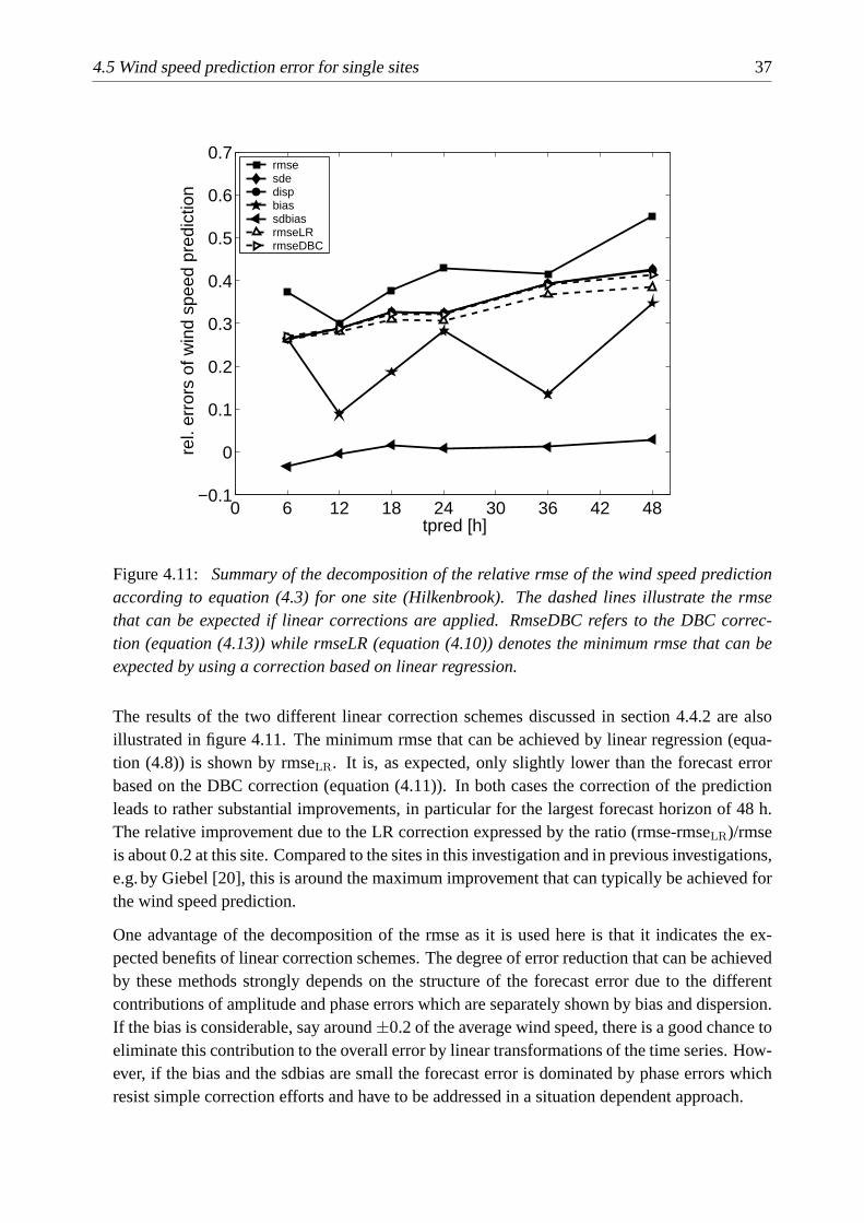
4.5 Wind speed prediction error for single sites 37
0 6 12 18 24 30 36 42 48−0.1
0
0.1
0.2
0.3
0.4
0.5
0.6
0.7
tpred [h]
rel
. err
ors
of w
ind
spee
d pr
edic
tion
rmsesdedispbiassdbiasrmseLRrmseDBC
Figure 4.11: Summary of the decomposition of the relative rmse of the wind speed predictionaccording to equation (4.3) for one site (Hilkenbrook). The dashed lines illustrate the rmsethat can be expected if linear corrections are applied. RmseDBC refers to the DBC correc-tion (equation (4.13)) while rmseLR (equation (4.10)) denotes the minimum rmse that can beexpected by using a correction based on linear regression.
The results of the two different linear correction schemes discussed in section 4.4.2 are alsoillustrated in figure 4.11. The minimum rmse that can be achieved by linear regression (equa-tion (4.8)) is shown by rmseLR. It is, as expected, only slightly lower than the forecast errorbased on the DBC correction (equation (4.11)). In both cases the correction of the predictionleads to rather substantial improvements, in particular for the largest forecast horizon of 48 h.The relative improvement due to the LR correction expressed by the ratio (rmse-rmseLR)/rmseis about 0.2 at this site. Compared to the sites in this investigation and in previous investigations,e.g.by Giebel [20], this is around the maximum improvement that can typically be achieved forthe wind speed prediction.
One advantage of the decomposition of the rmse as it is used here is that it indicates the ex-pected benefits of linear correction schemes. The degree of error reduction that can be achievedby these methods strongly depends on the structure of the forecast error due to the differentcontributions of amplitude and phase errors which are separately shown by bias and dispersion.If the bias is considerable, say around±0.2 of the average wind speed, there is a good chance toeliminate this contribution to the overall error by linear transformations of the time series. How-ever, if the bias and the sdbias are small the forecast error is dominated by phase errors whichresist simple correction efforts and have to be addressed in a situation dependent approach.

38 4 Assessment of the overall prediction uncertainty
4.6 Power prediction error for single sites
After the overall prediction accuracy of the wind speed prediction has been assessed in theprevious section the prediction of the power output is evaluated in the following. In order tocompare different sites the assessment of the power prediction error also requires some kind ofnormalisation. In this investigation the annual mean of the measured power output is taken asreference value because it inherently considers both the machine type with its rated power andthe typical wind speeds at the location. Table 4.3 shows details concerning the turbines that areinstalled at the six selected sites. The given mean values refer to the year 1996.
Table 4.3: Rated power and annual mean values of measured power output of the wind turbinesat the selected sites with corresponding standard deviation. The relative standard deviation isbetween 0.99 and 1.40, i.e. it is by a factor 1.8 to 2.6 larger than the corresponding wind speedresult.
site name rated power mean measured standard deviation of relative standardpower output measured power output deviation
[kW] Pmeas [kW] σ(Pmeas) [kW] σ(Pmeas)/Pmeas
Altenbeken 150 30.2 37.9 1.25Fehmarn 200 59.8 59.5 0.99Hilkenbrook 80 12.0 16.7 1.39Rapshagen 300 48.8 58.8 1.20Schuelp 250 46.0 59.6 1.30Soelmnitz 200 25.4 35.6 1.40
The relative standard deviation,σ(Pmeas)/Pmeas, of the measured power output in table 4.3 is bya factor 1.8 to 2.6 larger than the relative standard deviation,σ(umeas)/umeas, of the time seriesof the wind speed measurement. This factor is due to the power curve and can be regarded as theeffective non-linearity factor that describes the scaling of variations in the wind speed due to thelocal slope of the power curve as already mentioned in section 2.4. IfP (u) was proportional tou3 and the variations inu were small compared to the mean value, the ratio between the relativestandard deviations of power output and wind speed would be around 3 corresponding to theaverage relative derivative.
The power predictions used here were calculated as described in section 2.4 based on DWD’snumerical wind speed prediction. Analogous to the statistical analysis of the wind speed fig-ures 4.12 to 4.16 show the different relative error measures versus prediction time.
The relative rmse of the power prediction (figure 4.12) is in the range of 0.5 to 1.1 for 6 h and0.8 to 1.45 for 48 h. Hence, its overall level is about two times larger than the relative rmse ofthe wind speed.
In figure 4.13 the relative bias shows a rather large discrepancy between the different sitesfrom 0.8 to -0.5 being considerably more pronounced compared to wind speed. The diurnalvariations are still of the order 0.1 to 0.2 but mostly inverse with maximum bias at noon ratherthan midnight. Thus, the characteristic “W”-shape of the wind speed bias is lost (cf. figure 4.7).

4.6 Power prediction error for single sites 39
0 6 12 18 24 30 36 42 480
0.5
1
1.5
2
tpred [h]
rel
. rm
se o
f pow
er p
redi
ctio
n
FehmarnHilkenbrookSchuelpAltenbekenRapshagenSoellmnitz
Figure 4.12: Relative root mean square error (rmse) between predicted and measured poweroutput for the selected sites in the year 1996. The rmse seems to increase with increasingforecast horizon. There is no apparent coherent behaviour among the different sites.
0 6 12 18 24 30 36 42 48−1
−0.5
0
0.5
1
tpred [h]
rel
. bia
s of
pow
er p
redi
ctio
n
FehmarnHilkenbrookSchuelpAltenbekenRapshagenSoellmnitz
Figure 4.13: Relative bias of the mean values of predicted and measured power output forthe same sites as in figure 4.6. The diurnal variations are inverse compared to the wind speedbias in figure 4.7. Sites located in flat terrain have positive bias (solid symbols) while sites incomplex terrain tend to have negative bias (white symbols).

40 4 Assessment of the overall prediction uncertainty
0 6 12 18 24 30 36 42 480
0.5
1
1.5
2
tpred [h]
rel
. sde
of p
ower
pre
dict
ion
FehmarnHilkenbrookSchuelpAltenbekenRapshagenSoellmnitz
Figure 4.14: Relative sde of the power prediction for the selected sites. Again the increaseof sde with prediction time can be observed. The differences between rmse (figure 4.12) andsde of the power prediction is rather small for most sites. Hence, in contrast to the wind speedprediction (figures 4.6 and 4.8) the sde dominates the rmse with a smaller contribution of thebias.
The inversion of the diurnal variations compared to wind speed indicates that the differencebetween mean values at daytime and nighttime is overestimated by the power prediction system.This is mainly due to the fact that stability effects are not included in the transformation to hubheight (equation 2.4). As shown by Focken [14] this can lead to an overestimation of the windspeed prediction, and hence the power prediction, in situations of unstable thermal stratificationwhich typically occur during daytime. Another influence on the bias of the power prediction isexpected by the non-linearity of the power curve as the difference between the mean values ofprediction and measurement at noon grows larger than at midnight because the midday meanshave larger absolute values.
As before the sign of the bias seems to be connected to the terrain type. While flat terrain siteshave positive bias those in more complex terrain provide negative values. Thus, the generalunderestimation or overestimation, respectively, of sites according to the terrain is still presentand enhanced by converting wind speed to power.
It can be seen in figure 4.14 that the relative sde, i.e. the standard deviation of the power predic-tion error, does not differ much from the relative rmse in figure 4.12. So in contrast to the windspeed prediction sde dominates the rmse with a smaller contribution of the bias.
The relative sdbias of the power prediction (figure 4.15) is similar to the wind speed predictionconcerning the behaviour of the individual sites. Again being in complex terrain (Altenbeken,Soellmnitz and Rapshagen) leads to a general underestimation of the fluctuations of the mea-sured power signal while it is vice versa for flat terrain (Fehmarn, Schuelp and Hilkenbrook).

4.6 Power prediction error for single sites 41
0 6 12 18 24 30 36 42 48−1
−0.5
0
0.5
1
tpred [h]
rel
. sdb
ias
of p
ower
pre
dict
ion
FehmarnHilkenbrookSchuelpAltenbekenRapshagenSoellmnitz
Figure 4.15: Difference between standard deviations of predicted and measured power output(sdbias) normalised with mean power output for the selected sites. As in figure 4.7 the threeflat terrain sites group together in the range of small sdbias. Unlike Altenbeken with a stronglynegative sdbias.
0 6 12 18 24 30 36 42 480
0.5
1
1.5
2
tpred [h]
rel
. dis
p of
pow
er p
redi
ctio
n
FehmarnHilkenbrookSchuelpAltenbekenRapshagenSoellmnitz
Figure 4.16: The relative dispersion of the power prediction is in a rather narrow range forthe selected sites. It increases with prediction time with a similar rate at all sites indicating asystematic phase error that affects different sites in the same way.
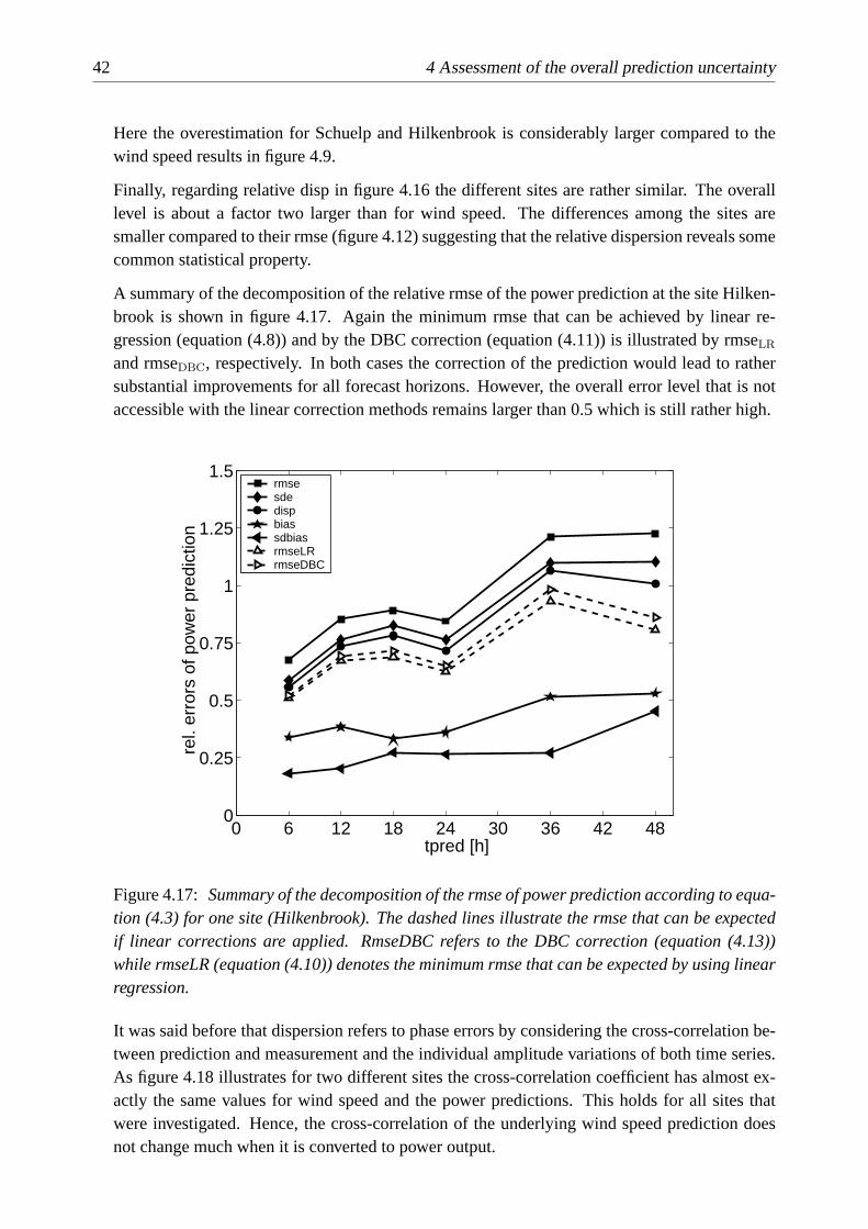
42 4 Assessment of the overall prediction uncertainty
Here the overestimation for Schuelp and Hilkenbrook is considerably larger compared to thewind speed results in figure 4.9.
Finally, regarding relative disp in figure 4.16 the different sites are rather similar. The overalllevel is about a factor two larger than for wind speed. The differences among the sites aresmaller compared to their rmse (figure 4.12) suggesting that the relative dispersion reveals somecommon statistical property.
A summary of the decomposition of the relative rmse of the power prediction at the site Hilken-brook is shown in figure 4.17. Again the minimum rmse that can be achieved by linear re-gression (equation (4.8)) and by the DBC correction (equation (4.11)) is illustrated by rmseLR
and rmseDBC, respectively. In both cases the correction of the prediction would lead to rathersubstantial improvements for all forecast horizons. However, the overall error level that is notaccessible with the linear correction methods remains larger than 0.5 which is still rather high.
0 6 12 18 24 30 36 42 480
0.25
0.5
0.75
1
1.25
1.5
tpred [h]
rel
. err
ors
of p
ower
pre
dict
ion
rmsesdedispbiassdbiasrmseLRrmseDBC
Figure 4.17: Summary of the decomposition of the rmse of power prediction according to equa-tion (4.3) for one site (Hilkenbrook). The dashed lines illustrate the rmse that can be expectedif linear corrections are applied. RmseDBC refers to the DBC correction (equation (4.13))while rmseLR (equation (4.10)) denotes the minimum rmse that can be expected by using linearregression.
It was said before that dispersion refers to phase errors by considering the cross-correlation be-tween prediction and measurement and the individual amplitude variations of both time series.As figure 4.18 illustrates for two different sites the cross-correlation coefficient has almost ex-actly the same values for wind speed and the power predictions. This holds for all sites thatwere investigated. Hence, the cross-correlation of the underlying wind speed prediction doesnot change much when it is converted to power output.

4.6 Power prediction error for single sites 43
With the definition of the dispersion in equation (4.3) the doubling of the relative dispersionis caused by the standard deviationsσ(Ppred) andσ(Pmeas) which are relatively 2 to 2.5 timeslarger thanσ(upred) andσ(umeas) (cf. tables 4.2 and 4.3). This factor can be considered as theeffective non-linearity factor of the power curve. If the power curve followedu3 this factorwould be around 3.
0 6 12 18 24 30 36 42 480.5
0.6
0.7
0.8
0.9
1
tpred [h]
cro
ss−
corr
elat
ion
coef
ficie
nt
Altenbeken wind speedHilkenbrook wind speedAltenbeken powerHilkenbrook power
Figure 4.18: Cross-correlation coefficients for the different prediction times of wind speed andpower prediction at two different sites. Altenbeken has a comparatively low cross-correlationwhile Hilkenbrook is among the sites with the highest values. At both sites there are only smalldifferences between the two prediction types. This holds for all all sites in this investigation. Thecross-correlation suffers only minor changes by converting wind speed to power output usingthePrevientosystem.
The large standard deviations of the measured power time series at a site are, of course, deter-mined by the specific turbine and the local wind conditions. The prediction system is designedto match the measured time series as exactly as possible. Hence, it should provide the samemean and standard deviation as the “real” time series together with a correlation close to 1. Inthis case the dispersion provides a lower boundary to the rmse for a given cross-correlation.This threshold is rather high in the case of the power prediction that already ranges up to 100%of the mean power output for the 48 h forecast. It is important to note that this level can only bereduced by improving the cross-correlation. Changes in bias and sdbias can optimise the powerprediction only in a limited range.
In addition, figure 4.18 shows that the cross-correlation coefficients decay almost linearly withthe forecast horizon. Note that each of these coefficients has been calculated separately withdata points of one prediction time only.

44 4 Assessment of the overall prediction uncertainty
The decreasing cross-correlation coefficients indicate that as expected the mismatch between theprediction of the NWP and local measurement grows systematically with prediction horizon.Such a linear decay also occurs for the cross-correlation function of two rectangles. So, theincreasing divergence between prediction and measurement can be imagined as the decreasingoverlap between two rectangles that are moved apart at a constant speed where the overlaprepresents the degree of correct information in the prediction. With the data in figure 4.18 thetime constant of this process would be about 230 hours, i.e. 9.5 days. However, this analogyshould not be overtaxed as the mechanism that leads to the decreasing correlation is related tothe decreasing correspondence between the three dimensional patterns of the predicted and the“real” atmospheric state due to advection, i.e. the shift between the patterns, and defects, i.e.local differences between the patterns. The correlation-coefficients derived from the local timeseries used in this investigation represent the resulting effect of these spatial phenomena and donot distinguish the type of process that dominates the increasing mismatch between predictionand measurement.
Comparison with persistence
The DM prediction of wind speed is tested against persistence to compare the accuracy to a verysimple reference system in order to get an impression about the different behaviour of the two.A persistence prediction is made by using the measurement value at 00 UTC as forecast valuefor the whole prediction horizon. Thus, the current value is assumed not to change in the nearfuture, i.e. to persist over the forecast interval. Persistence was chosen as reference becauseit inherently contains information about the actual meteorological situation at the site shortlybefore the prediction horizon begins.
It can be concluded from the relative dispersion in figure 4.19 that the prediction of a NWPhas a better performance than persistence for prediction times above 6 h. This is a well-knownfact for numerical prediction systems, e.g. Landberg [29] and Giebel [20] showed that below6 h persistence is in fact better. The reason for this behaviour might be related to a relaxationprocess with decaying transients in the NWP after the initial conditions are set and the run isstarted. The results for the power forecast are comparable.
Note that for forecast horizons larger than about 15 hours the climatological mean of the windspeed is a more suitable reference system than persistence. This is due to the fact that the errorof the persistence forecast is by construction determined by the auto-correlation function of thewind speed, which decays approximately exponentially with a time constant around 15 hours,and, therefore, the persistence forecast is rather uncorrelated after this time period. Hence, anew reference model based on the superposition of persistence for short forecast horizons andthe climatological mean for longer forecast horizons has been proposed by Nielsen et al. [46].Though the use of this new reference model would reduce the difference between the errorsof NWP forecast and the reference forecast by a few percent, the wind speed prediction of theNWP is still significantly better.

4.7 Conclusion 45
0 6 12 18 24 30 36 42 480
0.2
0.4
0.6
0.8
1
tpred [h]
rel
. dis
p of
win
d sp
eed
pred
ictio
n
Fehmarn prediction NWPHilkenbrook prediction NWPFehmarn persistenceHilkenbrook persistence
Figure 4.19: Comparison between the relative dispersion of the persistence prediction of thewind speed, where the current measurement value is assumed not to change over the predictionhorizon, and the NWP wind speed prediction. For lead times above about 6 h the predictiongenerated by the NWP performs significantly better than persistence.
4.7 Conclusion
The decomposition of the root mean square error (rmse) into different components provides con-siderable insight into the different origins of deviations between prediction and measurement.The contributions of the difference of the mean values (bias), the difference of the standarddeviations (sdbias) and the dispersion (disp) to the rmse reveal some general statistical featuresof the errors that allow to distinguish local effects from global properties.
Concerning local effects the results strongly suggest that the terrain type has a systematic in-fluence on the bias and the sdbias. For the wind speed as well as the power prediction sitesin flat terrain tend to have positive bias and small sdbias while sites in complex terrain aremore inclined towards negative bias and sdbias. The reason for this is thought to originate fromthe fact that the NWP uses a meso-scale roughness length which represents the typical surfaceroughness including orography within the grid cell and not the local situation at the position ofthe wind farm. In particular, in complex terrain the wind turbines are systematically erected at“optimal” locations, i.e. on top of hills rather than in valleys. This might lead to the generalunderestimation of these sites by the prediction. Hence, a general overestimation or underesti-mation, respectively, by the prediction can be attributed to the on-site conditions. However, inthis investigation the terrain type was classified very roughly without quantitatively relating thebehaviour of the bias and sdbias to orography.
Diurnal variations occur mainly in the bias indicating imperfect modelling of atmospheric strat-ification by the NWP. With regard to the bias of the wind speed most of the inland sites show a

46 4 Assessment of the overall prediction uncertainty
typical ”W”-shape where at midnight the relative bias is about 10-20% larger than at noon. Atthe island site this effect is weak. The bias of the power prediction is still of the order 10% of theaverage annual power output but does not reproduce the “W”-shape as the diurnal variations arereversed which is mainly caused by neglecting the effects of thermal stratification in calculatingthe wind speed at hub height.
Regarding relative dispersion, in particular for the wind speed prediction, different sites showa very consistent behaviour indicating a general property that affects all locations in the sameway. The linear increase of the dispersion with prediction horizon has comparable slopes forthe majority of sites and describes the systematic growth of the average phase errors betweenprediction and measurement with increasing lead time.
The contribution of dispersion to the forecast error plays an important role. In contrast to thebias and the sdbias it cannot simply be calibrated out by linear transformations of the completetime series as the dispersion involves the cross-correlation which is invariant under transforma-tions of that kind. In this sense the dispersion provides an estimate of the lower boundary of theprediction error and limits the space for “simple” improvements.
Compared to the wind speed prediction the relative dispersion of the power prediction is bya factor of 1.8 to 2.6 larger. As the cross-correlation does not change by converting the windspeed prediction to power this increase in dispersion is mainly caused by increased fluctuations,σ(Ppred) andσ(Pmeas), of the predicted and measured power time series. Hence, the factormainly represents the effective non-linearity of the power curve that unavoidably amplifies thewind speed fluctuations. Because larger amplitude variations are punished by a higher disper-sion the prediction error of the power prediction automatically increases compared to the windspeed prediction. Thus, the relatively large error of the power prediction system is not mainlycaused by the additional errors associated with the modelling used in the power prediction sys-tem, e.g. local refinement. Of course, the procedure that calculates the predicted power hasto be as precise as possible but the crucial point is that the high error level of the power pre-diction more or less directly reflects the accuracy of the underlying wind speed prediction incombination with the influence of the non-linear power curve.
The lesson learned from this chapter is that converting a wind speed prediction to a power pre-diction fundamentally changes the statistical properties of the prediction error. Most of thesechanges can be be blamed on the non-linearity of the power curve. The error of the power pre-dictions has a non-Gaussian distribution while the underlying wind speed errors are distributednormally in most cases. The prediction of the power output naturally has a larger error com-pared to the wind speed. Hence, the power prediction system primarily has to avoid additionalerrors to prevent things going from bad to worse. Correction schemes based on linear regressiontechniques that are applied globally to the time series are expected to be of little use to dramati-cally decrease the forecast error. One way out of this situation seems to focus on situation-basedimprovements of the wind speed prediction. This would require to work directly on the NWPand enhance its performance with respect to an accurate modelling of the wind speed.

5 Smoothing effects in regional power prediction
Abstract
The investigation in this chapter focuses on the statistical analysis of the power prediction error of an
ensemble of wind farms compared to single sites. Due to spatial smoothing effects the relative prediction
error decreases considerably. Measurements of the power output of 30 wind farms in Germany show that
as expected this reduction depends on the size of the region. To generalize these findings an analytical
model based on the spatial correlation function of the prediction error is derived to describe the statistical
characteristics of arbitrary configurations of wind farms. This analysis reveals that the magnitude of the
error reduction depends only weakly on the number of sites and is mainly determined by the size of the
region, e.g. for the size of a typical large utility (approx. 730 km in diameter) less than 100 sites are
sufficient to have an error reduction of about 50%.
5.1 Introduction
In the previous chapter the typical forecast errors in terms of wind speed and power output areevaluated for single sites. However, in practical use transmission system operators or electricitytraders are mainly interested in the total amount of wind energy to be expected in their supplyarea for the days to come. Therefore, a prediction of the combined power output of many windfarms distributed over a large region is required. By integrating over an extended area the errorsand fluctuations underlying the measurement and the forecast at single sites cancel out partly.These statistical smoothing effects lead to a reduced prediction error for a region compared toa local forecast. In this chapter the smoothing effects are investigated in greater detail. Theanalysis of measured data very clearly shows a reduction of the error but is constrained to afixed ensemble of sites. This restriction is overcome by using model ensembles of ficticioussites together with an analytical description of the spatial correlation of the forecast error. Thus,the main parameters that determine the magnitude of the error reduction, namely the size of theregion and the number of sites it contains, can easily be varied. The aim is to quantitativelydescribe the error reduction by spatial smoothing effects for typical wind farm configurationsand region sizes. For this purpose the error reduction will mainly be described by the ratiobetween the forecast error of the regional prediction and the typical forecast error of a singlesite.
5.2 Ensembles of Measurement Sites
The first approach is to investigate the spatial smoothing effects using measured data from anensemble of 30 wind farms in the Northern part of Germany. The sites are divided into regionsof two different types according to typical areas covered by a medium and a large utility. Thesmaller regions with a diameter of approximately 140 km (see figure 5.1) contain three to five

48 5 Smoothing effects in regional power prediction
measurement sites each. The larger regions are about 350 km in diameter with five to sevensites each. For comparison a very large region containing all sites which has a size of about 730km is formed.
Figure 5.1: Regions in Northern Germany with 140 km in diameter. The points denote themeasurement sites.
The predicted and measured power output of a region is calculated by summing up the timeseries for every wind farm located in the region and dividing them by the number of windfarms. Similar to the verification analysis of single sites the standard deviation,σensemble, of thedifference between these two ensemble time series, i.e. the sde as defined in equations (4.1) and(4.4), gives the regional prediction error. Figure 5.2 shows the results for the different regionsizes and various prediction times. The standard deviation,σensemble, of the ensemble, i.e. theregional prediction error, is normalised to the mean standard deviation of the single sites,σsingle
according to chapter 4, and averaged over all regions of the same size. For the given ensemblethis ratio decreases with increasing region size, e.g. the 6 h prediction gives an average ratioof 0.79 for the 140 km region, 0.68 for the 350 km region, and 0.50 for the 730 km region(figure 5.2). In all cases the reduction of the regional prediction error is less pronounced forlarger prediction times.
5.3 Model ensembles
The analysis for the specific set of measurement sites shows a significant decrease of the pre-diction error compared to a single site. In order to draw general conclusions concerning otherconfigurations of wind farms random ensembles of fictitious sites are used. Thus, the size of theregions and the number of wind farms can be varied over large ranges to see how the reduction

5.3 Model ensembles 49
0
0.2
0.4
0.6
0.8
1
6 12 18 24 30 36 42 48
σ ens
embl
e/σ s
ingl
e
prediction time [h]
140 km350 km730 km
Figure 5.2: Ratio between standard deviations of error for ensemble and single prediction(σensemble/σsingle) for various region sizes and forecast horizons for the ensemble of measurementsites. σensemble/σsingle decreases with increasing region size. In all cases the reduction of theregional prediction error is less pronounced for larger prediction times.
of the error depends on these parameters. For this purpose it is necessary to establish a properstatistical description of the regional prediction error.
The key elements connecting the spatial distribution of sites with the regional prediction errorare the cross-correlation coefficientsrxy of the time series of the pointwise error, i.e.εP(t) :=
Ppred(t) − Pmeas(t), between pairs of single sites. Ifrxy is known for all pairs of sites, theregional forecast error,σensemble, can easily be calculated usingσ of the individual sites by
σ2ensemble =
1
N2
∑x
∑y
σxσyrxy (5.1)
whereN is the number of sites in the region,σx the standard deviation of the single sites.
To obtain an analytic function describing the dependence ofrxy on the site distance the follow-ing procedure is applied. For each pair of the 30 wind farms the cross-correlation coefficientbetween pointwise prediction errors is calculated and ordered according to the distance betweenthe two sitesx andy. Figure 5.3 shows cross-correlation coefficients versus distance for thevarious forecast horizons where the data points have been averaged over 25 km bins. For smallprediction times (6 and 12 h) the cross-correlation decreases rather rapidly within 150 km whilefor longer times (36 and 48 h) the decrease is much slower. This might be due to the growingsystematic errors for increasing forecast horizon which give rise to higher spatial correlations.
Note that the spatial cross-correlation coefficients of the measured power alone decay consider-ably slower with increasing distance than the cross-correlation of the deviations. As shown byBeyer et al.[6] the cross-correlation of the power output of wind turbines is about 0.7 at 130 km

50 5 Smoothing effects in regional power prediction
-0.2
0
0.2
0.4
0.6
0.8
1
0 100 200 300 400 500 600
cros
s-co
rrel
atio
n
distance [km]
deviation 06 hdeviation 12 hdeviation 36 hdeviation 48 h
prediction 36 h
Figure 5.3: Spatial cross-correlation of prediction error for various prediction times. Thecross-correlation coefficients have been averaged over 25 km bins. The values do not go through1 for d = 0 because the distances of wind turbines belonging to the same wind farm are notresolved. For comparison the cross-correlation function of the prediction alone is also shownwhich decays significantly slower than the error.
while at the same distancerxy drops to approx. 0.2 for the 6 h prediction (figure 5.3). Hence,due to the large-scale weather patterns which simultaneously affect many wind farms the spatialcorrelation of the power output is considerably higher than that of the power prediction error.
The cross-correlation of the regional prediction error is approximated by fitting analytic func-tions of the formrxy = a · e−d/b (a andb are fit-parameters andd is the distance between thetwo sites) to the cross-correlation coefficients derived from the measured data. It turns out thatpiecewise exponentials lead to a suitable fit to the data points. Now the correlation functionrxy
based on the fitted data together with equation (5.1) allow for calculating the prediction error,σensemble, of the model regions with fictitious wind farms. The individual forecast errorsσx
of the fictitious wind farms are assumed to be equal which means that they all have the sameweight. The geographical coordinates of the model ensembles are chosen randomly. Each resultgiven in the following represents an average value over ten realisations of ensembles with fixedsize and number of sites.
Figure 5.4 shows the ratio between the regional error and the mean of single sites,σensemble/σsingle for two regions with different sizes versus the number of sites in the region. Thecross-correlation functionrxy based on the 36 h forecast was used. Obviously,σensemble/σsingle
approaches a saturation level for increasing number of wind farms. This limit is already reachedfor a rather small number of wind farms. Beyond that point the error reduction does practicallynot depend on the number of sites, e.g. for the size of a typical large utility (approx. 730 km)about 100 sites are sufficient to have a constant level of 0.49.

5.3 Model ensembles 51
0
0.2
0.4
0.6
0.8
1
0 200 400 600 800 1000
σ ens
embl
e/σ s
ingl
e
number of wind turbines
370 km730 km
Figure 5.4: Ratioσensemble/σsingle versus number of sites for the model ensembles. Each data-point represents an average over 10 ensembles. The fitted cross-correlation function for the 36hforecast was used. A saturation level is reached for a relatively small number of sites.
0
0.2
0.4
0.6
0.8
1
0 2 4 6 8 10 12 14 16 18 20
σ ens
embl
e/σ s
ingl
e
number of wind turbines
370 km730 km
uncorrelatedlimit 370 kmlimit 730 km
Figure 5.5: Same as fig. 5.4 but with theN− 12 behaviour of uncorrelated sites. The constant
lines indicate the limit values of the model regions. The intersection of these lines withN− 12
provides the number of uncorrelated sources that would lead to the same error reduction.

52 5 Smoothing effects in regional power prediction
For uncorrelated sources one would expectσensemble/σsingle= N− 12 showing no saturation for
largeN . Let the limit value for a model region beσsat then the number of uncorrelated sourceswith at least the same signal to noise ratio is simply given by
N = int(σ−2
sat
)+ 1
where the operatorint truncates the digits. As illustrated in figure 5.5 the limit value of thelargest region with 730 km in diameter corresponds to about 5 (exactly 4.15) uncorrelatedsources and the one of the smaller region to 3 (2.51). Thus, due to the finite correlations ofthe prediction error between distant sites the regional error reduction is far less pronouncedthan for uncorrelated sites.
The experimental data of section 5.2 agree very well with these calculations. Comparing the36 h data in figure 5.2 with the values corresponding to the same number of sites, i.e. 30, infigure 5.4 givesσensemble/σsingle = 0.71 for the 360 km region for both ensembles. For the 730km this ration is 0.53 for the ensemble of measurement sites and 0.52 for the model ensembles.
As expected the saturation level decreases with increasing size of the region. This is illustratedin figure 5.6 where the limit values for regions with different extensions containing 4000 sitesare shown. There is a rapid decay for extensions below 500 km.
0
0.2
0.4
0.6
0.8
1
0 500 1000 1500 2000
σ ens
embl
e/σ s
ingl
e
region size [km]
Figure 5.6: Saturation values ofσensemble/σsingle (4000 sites) for the 36 h forecast. Eachdata-point represents an average over 10 ensembles. The dashed line illustrates the ratio,σensemble/σsingle determined for the ensemble of all wind farms in Germany.
The distribution of distances within the ensemble of wind farms plays a crucial role in ex-plaining the saturation level. Figure 5.7 shows typical frequency distributions of the distancesin a 360 km region for different numbers of randomly distributed wind farms. The distribu-tions correspond to specific ensembles, i.e. another realisation has a different distribution. Fig-ure 5.7 clearly indicates that the distribution functions converge for an increasing number of

5.3 Model ensembles 53
wind farms. Beyond a certain number of wind farms in the region the characteristic distributionof distances approaches a limit distribution such that the regional error given by equation (5.1)does no longer change. If the region has a certain “population density” of wind farms it con-tains enough pairs to represent all possible correlations which contribute toσensemble. Therefore,adding more sites to the region does not reduce the regional error, as would be expected for un-correlated sites, and a saturation is reached.
0
0.02
0.04
0.06
0.08
0.1
0 100 200 300 400
freq
uenc
y
distance [km]
20 wec100 wec500 wec
Figure 5.7: Frequency distribution of distances in the region with a diameter of 360 km. Thecurves represent randomly chosen coordinates of 20, 100 and 500 wind farms.
The limit distribution has a mean value which is typically about half the diameter of the region.As the distribution is concentrated around the mean most contributions toσensemble come fromthis interval. For increasing region size this leads to a decreasing saturation level due to theexponential decay of the cross-correlation function (figure 5.3).
Distribution of German wind farms
Finally, the real distribution of wind farms in Germany in the year 1999 is considered as aspecial model ensemble (figure 5.8) and the regional forecast error is compared to that of asingle site as above. For the 36 h prediction this givesσensemble/σsingle = 0.43. This ratio isillustrated by a dashed line in figure 5.6 giving a corresponding region size of 930 km whichrather exactly matches the north to south extension of Germany. Hence, this ratio agrees ratherwell with the theoretically found value.
Note that the imbalance in the distribution of sites in the North and South (figure 5.8) does notaffect the resulting error reduction factor,σensemble/σsingle as the critical number of around 100for a region of that size is, of course, exceeded.

54 5 Smoothing effects in regional power prediction
Figure 5.8: Distribution of wind turbines in Germany in 1999. The crosses denote ZIP-codeareas of the site locations.
5.4 Conclusion
The statistical smoothing effects of the prediction uncertainty that arise if a wind power pre-diction is made for a region with spatially distributed wind farms lead to a reduction of theprediction error of the aggregated power prediction compared to a single site. For an ensembleof wind farms where the analysis is based on measured data the improvement of the predictionis noticeable even for small regions and only few sites. Using model ensembles with randomlychosen locations permits to generalise the results in order to identify the impact of the two mainparameters, namely the spatial extension of the region and the number of sites it contains to-gether with their distribution. The magnitude of the reduction does strongly depend on the sizeof the region, i.e. the larger the region the larger the reduction. Concerning the number of sitescontained in the area a saturation level is already reached for a comparatively small number ofwind farms. This means that only few sites are sufficient to determine the magnitude of theimprovement of the power prediction.
The results of the analysis show that for regions with a sufficient number of preferably equallydistributed wind farms it is now possible to estimate the regional smoothing effect of the windpower prediction error by just considering the size of the region in question. As the errorreduction is due to statistical effects the power prediction for a region improves on average.However, single events like an incorrectly predicted storm front crossing the entire area lead toa coherent behaviour of the wind turbines. In this case the correlation of the prediction errorbetween the sites is, of course, higher than on average and spatial smoothing is less pronounced.
This investigation was carried out with measured data for northern Germany and output of the

5.4 Conclusion 55
NWP of the German weather service. The regions are characterised by mainly flat terrain withno mountains separating the area in different weather regimes. The parameters, especially thedecay length of the spatial cross-correlation of the deviations, are supposed to depend on thetypical length scales of the weather patterns crossing the region and on the numerical weatherprediction model which may have special characteristics. In the mid-latitudes where the weatherconditions are driven by high and low pressure systems the general patterns of circulation typesare comparable to our situation. Thus, the general behaviour of the cross-correlation functionbetween the sites which determines the degree of statistical smoothing and the saturation valuesshould be universal such that the qualitative results found in this investigation are applicable toother areas in the mid-latitudes as well.
The work on this chapter has been carried out together with U. Focken [14] and is published inFocken et al.[16].

56 5 Smoothing effects in regional power prediction

6 Assessment of wind speed dependent prediction error
Abstract
The investigations in this chapter follow the idea that the prediction error quantitatively depends on themeteorological situation that has to be predicted. As a first approach the wind speed as a main indicatorof the forecast situation is considered in greater detail. The probability density functions (pdf) of themeasured wind speeds conditioned on the predicted wind speed are found to be Gaussian in the rangeof wind speeds that is relevant for wind energy applications. An analysis of the standard deviations ofthese conditional pdfs reveals no systematic dependence of the accuracy of the wind speed predictionon the magnitude of the wind speed. With the pdfs of the wind speed as basic elements the stronglynon-Gaussian distribution of the power prediction error is explained underlining the central role of thenon-linear power curve. Moreover, the power error distribution can easily be estimated based on thestatistics of the wind speed, the wind speed forecast error, and the power curve of the turbine. Thus, itcan be reconstructed without knowing the actual measured power output which is interesting for futuresites or sites where no data is available. In addition, a simple formula based on linearising the standarddeviation of the error is derived. This model illustrates the dominating effect of small errors in the windspeed prediction being amplified by the local derivative of the power curve.
6.1 Idea behind detailed error assessment
The standard error measures that are used in the previous chapter are based on annual averagesof the data and provide only one constant value for each forecast time. However, there is reasonto believe that the magnitude of the error quantitatively depends on the meteorological situationthat is to be predicted. Thus, a more detailed view on the prediction error is required where themain parameters that characterise typical wind conditions have to be identified and related tothe corresponding forecast error.
The first candidate that can serve as an indicator of the forecast situation is the wind speed itself.It is a continuous parameter closely related to the forecast situation and the main input into thepower prediction system such that in this chapter the role of the predicted wind speed and itsprediction error are investigated more deeply.
As outlined in chapter 2 the chain of events seems rather straightforward: the initial uncertaintyintroduced by the error of the wind speed prediction is propagated through the power predictionsystem where it is mainly subject to changes by the power curve. Due to its non-linearity thepower curve is expected to amplify or damp initial errors in the wind speed according to itslocal derivative. And this derivative is a function of the wind speed. So clearly, the power curveis expected to be the key element that connects the errors of the wind speed prediction and thepower prediction. Thus, the major aim here is to derive a quantitative relation between the two.
The practical use of this relation and its implementation into a wind power prediction systemis to provide the user with additional information. First of all the prediction itself and secondly

58 6 Assessment of wind speed dependent prediction error
some indication concerning the reliability of the prediction. As financial losses might be pro-portional to the magnitude of the prediction error the inherent risk of faulty predictions must beknown for each forecast situation.
6.2 Introduction of conditional probability density functions
It was seen in section 4.3 that the probability density function,pdf(εu), of wind speed error isGaussian in most cases. As mentioned above a more detailed information concerning the errorto be expected in special conditions is desirable. Thus, a first approach is to refine the pdfs andlook at the statistical properties of the measured wind when the predicted wind speed is confinedto a certain value which from a mathematical point of view leads to conditional pdfs. In thissection the deviations of the measured wind speed from the predicted wind speed is investigatedin terms of these conditional pdfs.
Predicted and measured values of a meteorological variable at the same point of time and spaceare naturally not independent. In fact, they are supposed to be highly correlated as this is a majorprerequisite for an accurate prediction. The pairs(xpred, xmeas) are drawn simultaneously from ajoint distribution, pdf(xpred, xmeas), that characterises the statistical properties of the predictionand its error. This means that for arbitrary but fixed predicted valuesxpred the occurrences ofthe corresponding measured valuesxmeas are expected to be mainly concentrated in an intervalaroundxpred rather than being spread over the whole range of all possible values.
In the following investigation the “prediction perspective” is taken which means that the pre-dicted values are used as condition to the measurements. This aims at formulating the equationssuch that they can directly be used for prediction purposes.
Formally the conditional pdf of the wind speed is given by
pdf(umeas|upred) =pdf(upred, umeas)
pdf(upred)(6.1)
wherepdf(upred, umeas) is the joint distribution andpdf(upred) the unconditional, so-calledmarginal, wind speed distribution.
For practical purposes the time series are given by a finite number of data points with a certainaccuracy. So the probability function of the measured wind speedumeas under the conditionupred is approximately calculated by confining the prediction values to an interval aroundupred
and bin-counting the corresponding values forumeas.
The conditional pdfs can, of course, be used to obtain the unconditional distribution by
pdf(umeas) =
∫ ∞
0
pdf(umeas|upred) pdf(upred) dupred. (6.2)
These conditional pdfs of the wind speed can be used to reconstruct the error distribution,pdf(εu), of the wind speed prediction that was found in chapter 4. The conditional pdfs de-fined in equation (6.1) already contain all the information needed for that as they describe thedeviations between predicted and measured values. With the transformation
umeas 7→ εu where εu = upred − umeas (6.3)

6.2 Introduction of conditional probability density functions 59
the pdf(umeas|upred) are merely mirrored and shifted along the abscissa and transfered topdf(εu|upred). The original, unconditional error distribution can then be recovered by
pdf(εu) =
∫ ∞
0
pdf(εu|upred) pdf(upred) dupred. (6.4)
Note that if the conditional pdfs are approximately equal to each other and do not vary muchwith upred one obtainspdf(εu) ≈ pdf(εu|upred). In this case the overall pdfs of the error candirectly serve as conditional pdf.
Reconstructing the distribution of the power prediction error
Knowing the statistical properties of the wind speed is very helpful with regard to the predictionof the power output as the wind speed is the main input variable fed into the power predictionsystem. However, as seen in chapter 4 the error distributions of the power prediction differqualitatively from those of the wind speed in that they are neither Gaussian nor approximatelyGaussian which is mainly due to the non-linear power curve of the wind turbines. The followinginvestigation focuses on the role of the power curve in transforming the distributions of the windspeed and its error into those of the power output.
In figure 6.1 a typical power curve,P (u), is shown with cut-in speed around4 m/s followedby a sharp increase of power over the interval5 − 10 m/s and a saturation at the level ofrated power for higher wind speeds. Let∆u be a small interval around the wind speedu and∆P = P (u + ∆u) − P (u) the resulting difference in the power output. For small∆u thecorresponding∆P is then given by a Taylor-expansion aroundu:
∆P =dP
du(u)∆u. (6.5)
This equation generally describes how wind speed intervals are mapped to power intervals. If∆u is regarded as a small deviation between predicted and measured wind speed equation (6.5)illustrates that the power curve scales errors in the wind speed according to its local derivative.Thus, whether deviations in the wind speed are amplified or damped depends on the magnitudeof the wind speed.
Using equation (6.1) the probability to find a measurement valueu in the interval[umeas, umeas+
∆u] with upred confined to[upred, upred + ∆u] is
w := pdf(umeas|upred) pdf(upred) (∆u)2. (6.6)
If the area(∆u)2 around(umeas, upred) is mapped to(∆P )2 around(P (umeas), P (upred)) ac-cording to equation (6.5) the probabilityw is preserved because all events that are recorded inthe wind speed intervals also occur in the power output intervals. Hence,
w = pdf(umeas|upred) pdf(upred) (∆u)2
!= pdf(P (umeas)|P (upred)) pdf(P (upred)) (∆P )2
= pdf(P (umeas)|P (upred)) pdf(P (upred))
(dP
du(umeas)∆u
) (dP
du(upred)∆u
). (6.7)

60 6 Assessment of wind speed dependent prediction error
0 2 4 6 8 10 12 14 16 180
200
400
600
800
1000
u [m/s]
Pow
er [k
W]
Figure 6.1: Power curve of a pitch regulated wind turbine (solid line). For three different windspeeds conditional pdfs, pdf(umeas|upred,i), are illustrated on the x-axis which have mean=upred,i
and standard deviation 1. The corresponding pdf(P (umeas)|P (upred,i)) constructed from equa-tion (6.5) are plotted on the y-axis. The pdfs are not normalised for better visualisation. Forsmall and large wind speeds the Gaussian wind speed distributions are strongly deformed andno longer symmetric. For medium wind speeds the pdf of the power is significantly flatter andbroader than the pdf of the wind speeds.
If equation (6.7) is solved for the desired pdfs of the power output one obtains
pdf(P (umeas)|P (upred)) pdf(P (upred))
=pdf(umeas|upred) pdf(upred)
(dP
du(umeas)
)−1 (dP
du(upred)
)−1
. (6.8)
This equation provides the essential relation between the distributions of wind speed on theone hand and power on the other hand. As expected the power curve plays a crucial role inconnecting the statistical properties of both quantities. Note that the divergence in equation (6.8)for (dP/du)−1 → ∞ is compensated by∆P → 0 according to equation (6.5) such that theprobabilityw is always well defined.
Figure 6.1 illustrates the effect of equation (6.5) for three different Gaussian wind speed dis-tributions with same standard deviations. For small and large wind speeds the Gaussian windspeed distributions are strongly deformed and no longer symmetric. For medium wind speedsthe pdf of the power is significantly flatter and broader than the pdf of the wind speeds.
The next steps towards a full description of the statistics of the power prediction error in termsof the wind speed distributions are now right ahead: Equation (6.8) can be used to create the

6.2 Introduction of conditional probability density functions 61
functionspdf(P (umeas)|P (upred)) for eachP (upred). Then these functions are weighted ac-cording to the frequency distribution ofP (upred) and their variables are shifted analogous totransformation (6.3). Finally, these shifted functions are added and the unconditional pdf of thepower prediction error is reconstructed.
Equations (6.7) and (6.8) suggest that the basic elements in this reconstruction procedure canbe defined by
F (P (umeas), P (upred)) := pdf(umeas|upred) pdf(upred)
(dP
du(umeas)
)−1(dP
du(upred)
)−1
(6.9)
Note that this definition is an intermediate step that conveniently summarises all mathematicalterms involved. The functionsF contain the information how the conditional pdf of the windspeed has to be transformed to the corresponding power pdf and which weight this pdf has.Once the right-hand side of equation (6.9) has been usedF is defined in the power domain, i.e.the independent variables arePmeas := P (umeas) andPpred := P (upred).
The notationPmeas denotes the measured power obtained by plugging the measured wind speedat hub height into the theoretical power curve. Generally,Pmeas slightly differs from the directmeasurement of the power output,Pmeas, because the power curve of the local wind turbinemight deviate from the theoretical curve or additional errors that are not covered by the powercurve come in.
Analogous to the transformation of the conditional wind speed distribution in equation (6.3) thefirst variable in each of the functionsF is shifted according to
Pmeas 7→ εP where εP = Ppred − Pmeas. (6.10)
In the final step the unconditional distribution of the power prediction error is obtained by theintegration
pdfrec(εP ) =
∫ ∞
0
F (εP , Ppred) dPpred. (6.11)
Despite having a slight touch of looking complicated this method has some benefits. It ex-clusively provides the error statistics of the power prediction based on three ingredients: theconditional distributions of the wind speed prediction, the derivative of the power curve and thedistribution of the predicted wind speeds. For practical purposes these three components areeither given or can be estimated. The power curve is typically known numerically such thatthe derivative can easily be obtained. The distribution of the predicted wind speed is normallyprovided by the NWP output but if not it can be estimated from prediction data of nearby sitesor from Weibull distributions of the measurement data. If the conditional pdfs of the wind speedare not known for the site in question it can be assumed that they are Gaussian with mean valuesand standard deviations obtained by a qualified guess.
The concepts developed in the this section are now applied to data from real sites to check if therelations between the wind speed and the power distributions can be confirmed with finite setsof data points.

62 6 Assessment of wind speed dependent prediction error
6.3 Conditional PDF of wind speed data
The conditional pdfs of the wind speed are calculated as described by equation (6.1), i.e. thedistribution of the measured values is determined with the corresponding predicted value con-fined to a certain interval. The range of the occurringupred is divided into equidistant binswith width ∆u which is typically set to 1 m/s. The boundaries of the bins are given by[upred,i −∆u/2, upred,i + ∆u/2]. Hence,upred,i denotes the middle of the bins.
In figures 6.2 and 6.3 the conditional pdfs of the wind speed at two sites with different averagewind speeds are shown based on measured and predicted data of the year 1996. In these exam-ples the 36 h values of prediction and measurement are used but the qualitative behaviour of theother prediction times is comparable.
The distributions for small wind speeds are unsymmetric and far from being normal. This is dueto the fact that the wind speed is always positive and deviations fromupred,i are limited towardslower wind speeds but not towards larger ones. With increasingupred,i the pdfs become rathersymmetric.
Compared to a normal distribution with same mean and standard deviation these pdfs can beconsidered as being approximately Gaussian although the number of data points available perpdf is relatively small. Again the two statistical tests from chapter 4 are used to systematicallycheck the normality of the conditional pdfs. As expected the hypothesis that the pdf is Gaussianis rejected by theχ2-test and the Lilliefors-test for distribution functions with smallupred,i. Forlarger prediction values both tests indicate normality: in figure 6.2 for the pdfs with2.5 m/s ≤upred,i ≤ 6.5 m/s and in figure 6.3 for2.5 m/s ≤ upred,i ≤ 8.5 m/s.
It is apparent from figures 6.2 and 6.3 that in most cases the mean of the conditional pdfs doesnot correspond toupred,i which is related to the systematic errors in the data that already occurredin section 4.3. This is further illustrated in figure 6.4 where the means of the pdf(umeas|upred,i)are plotted versusupred,i. For Rapshagen (figure 6.4 (top)) the mean values are mostly abovethe diagonal, i.e. the predictions are on average smaller than the measurements, leading to anegative bias (c.f. figure 4.7). In contrast to this the majority of mean values for Fehmarn(figure 6.4 (bottom)) is below the diagonal which corresponds to an overall positive bias.
Forupred,i > 2 m/s the mean values increase linearly withupred,i but with slopes different fromunity indicating that the predictions systematically underestimate or overestimate the measure-ments. Within their error bars the mean values follow a line given by linear regression of alldata points except for largeupred,i where only few data points are available. Thus, the meanvalues of the conditional pdfs behave as expected in that they reflect, on a bin-wise level, thesystematic errors of the complete time series.
The pdfs in figure 6.2 and 6.3 seem to become wider for increasingupred,i suggesting that thedeviations ofumeas from upred,i, i.e. the prediction errors, grow on average which is equivalentto a decreasing forecast accuracy. This directly leads to the question if the accuracy of thewind speed prediction depends on the magnitude of the wind speed. In this investigation nofinal answer can be given as the behaviour for different sites and prediction times is ratherinconsistent.

6.3 Conditional PDF of wind speed data 63
u [m/s]0 1 2 3 4 5 6 7 8 9 10 11 12
0
0.4
0
0.4
0
0.4
0
0.4
0
0.4
0
0.4
0
0.4
0
0.4
0
0.4
Figure 6.2: Conditional probability density functions of 36 h wind speed values at site with lowaverage wind speed (Rapshagen). The different pdf(umeas|upred,i) (shaded areas) are stackedwhereupred,i has been varied in steps of 1 m/s, i.e.∆u = 1 m/s. The vertical line in each plotindicates the correspondingupred,i. For comparison a normal distribution having the same meanand standard deviation as pdf(umeas|upred,i) is shown (solid lines). For pdfs with2.5 m/s ≤upred,i ≤ 6.5 m/s the statistical tests indicate a Gaussian distribution. Note that conditionalpdfs for largeupred,i containing very few data points have been omitted.

64 6 Assessment of wind speed dependent prediction error
u [m/s]0 1 2 3 4 5 6 7 8 9 10 11 12 13 14 15
0
0.4
0
0.4
0
0.4
0
0.4
0
0.4
0
0.4
0
0.4
0
0.4
0
0.4
0
0.4
0
0.4
0
0.4
Figure 6.3: As figure 6.2 but for a high wind speed site (Fehmarn). Again the pdfs tend tobecome similar to normal distributions with increasingupred,i which is confirmed by the testsfor pdfs with2.5 m/s ≤ upred,i ≤ 8.5 m/s. Note that the number of data points decreases forlarger upred,i. and conditional pdfs containing very few data points have been omitted.

6.3 Conditional PDF of wind speed data 65
0 2 4 6 8 10 12 140
2
4
6
8
10
12
14
upred
[m/s]
[m/s
]
linear regressionmean(pdf(u
meas|u
pred))
0 2 4 6 8 10 12 140
2
4
6
8
10
12
14
upred [m/s]
[m/s
]
linear regressionmean(pdf(u
meas|u
pred))
Figure 6.4: The mean of pdf(umeas|upred,i) versusupred,i together with the actual data points(upred, umeas) for the 36 h prediction. Top: Rapshagen (cf. figure 6.2), bottom: Fehmarn (cf.figure 6.3). In both cases the mean values are located on the linear regression line based onthe data points forupred > 2 m/s. Their deviation from the diagonal (dashed line) reflects thesystematic errors.

66 6 Assessment of wind speed dependent prediction error
Consider the two examples for Rapshagen (figure 6.5 (top)) and Fehmarn (figure 6.5 (bottom)).While at Rapshagen (top) the relative standard deviation of the pdf(umeas|upred,i) has no apparenttrend and oscillates around the corresponding relative sde (see section 4.5), the pdf of Fehmarn(bottom) seems to have an increasing standard deviation. But such a clear trend cannot bedetected for other prediction times at this site.
0 2 4 6 8 10 12 140
0.1
0.2
0.3
0.4
0.5
0.6
upred [m/s]
rel
. std
(um
eas|
u pred
))
0 2 4 6 8 10 12 140
0.1
0.2
0.3
0.4
0.5
0.6
upred
[m/s]
rel
. std
(um
eas|u
pred
))
Figure 6.5: The standard deviations of pdf(umeas|upred,i) normalised by the mean measuredwind speed versusupred,i for Rapshagen (top) and Fehmarn (bottom). The prediction time isagain 36 h. The solid line illustrates the unconditional relative standard deviation of the error(cf. figure 4.8). The error bars provide the confidence intervals in calculating the standarddeviation of the conditional pdfs. While for Rapshagen no clear trend is detectable there seemsto be an increase of the relative standard deviations of the conditional pdfs with the predictedwind speed for Fehmarn. However, this is not systematic, neither for this prediction time atother sites nor for the other lead times at Fehmarn.

6.4 Estimating the distribution of the power prediction error 67
Generally, most sites show some variation of the standard deviation of pdf(umeas|upred,i) overupred,i with relative standard deviations that deviate of the order 0.1 from the unconditionalsde. The pdfs forupred,i ≤ 2 m/s are typically unsymmetric such that their standard deviationcannot be interpreted as 68%-confidence interval. Due to the limitation of these pdfs at thelower boundary their standard deviation is expected to be smaller compared to that one of thesymmetric pdfs.
These considerations lead to the result that there is only a weak, if any, systematic dependenceof the accuracy of the wind speed prediction on the wind speed.
6.4 Estimating the distribution of the power prediction error
In this section it is shown that the distribution of the power output can indeed be derived fromthe conditional pdfs of the wind speed together with the power curve. Based on the empiricalpdfs of the wind speed found in the above section the unconditional distribution of the powerprediction error can be reconstructed.
First of all, the quality of the reconstruction procedure is tested against a synthetic error distri-bution, denoted aspdftest(εP ), generated by usingεP := P (upred) − P (umeas), i.e. using thetheoretical power curve only. As figure 6.6 demonstrates for Rapshagen the reconstruction ofthe error distribution that was calculated with equations (6.9) and (6.11) and the conditionalpdfs of the wind speed obtained in the last section (figures 6.2 and 6.3) almost exactly recov-erspdftest(εP )). Thus, though the procedure of first decomposing the wind speed data intoconditional distributions, scaling them with the reciprocal derivative of the power curve andreassembling everything again leaves some space for numerical artefacts and inaccuracies dueto small data sets it is robust enough to produce the expected results.
To be of practical use the more interesting test of the reconstruction is against the “real” dis-tribution, pdfreal(εP ), of the prediction error. Figure 6.7 shows the estimatedpdfrec(εP ) forRapshagen (top) compared to the distribution,pdfreal(εP ), of the forecast error based on mea-surements of the actual power output. The overall agreement between the two distributions israther good except for smallεP . The reconstructed pdf covers the typical features of the orig-inal distribution in that it is unsymmetric in the same way and has the typical peak for smalldeviations.
As the error bars ofpdfreal(εP ) indicate the reconstructed distribution does not perfectly matchthe real one in all of the bins, in particular for Fehmarn (figure 6.7 (bottom)). This deviationindicates additional sources of error that are not covered by considering the power curve effectonly.
The results so far explain how the power prediction errors are statistically distributed and whythe distribution has this special shape. If measured and predicted data of the power output areavailable there is no point in putting any effort in calculating the reconstructedpdfrec(εP ) asthe error distribution is already available. However, if no data or only wind speed data is athand the reconstruction can be used to get an idea how the error distribution of the power mightlook like. The minimum requirements to calculate this estimated distribution comprise fourimportant aspects: First, the reasonable assumption that the conditional pdfs of the wind speed

68 6 Assessment of wind speed dependent prediction error
−0.5 −0.25 0 0.25 0.50
1
2
3
4
5
6
7
εP / rated power
(εP)
pdftest
pdfrec
Figure 6.6: Consistency check of the reconstruction procedure according to equations (6.9)and (6.11) for the 36 h prediction at Rapshagen.εP is normalised to the rated power.The reconstructedpdfrec(εP ) is compared topdftest(εP ) which is based on evaluatingεP :=
P (upred) − P (umeas). These two pdf should be identical. However, they show small deviationsfor the bins aroundεP = 0.
are all Gaussian (as discussed in section 6.3) with the same standard deviation,σ(εu). Second,a qualified guess concerning the value ofσ(εu), e.g. from the weather service, as in [55], ornearby sites. Third, the distribution of the wind speeds at the desired site and, finally, the powercurve of the wind turbine has to be available.
With the considerations of this section the conditional pdfs, pdf(εP |Ppred), can in principle beconstructed and, hence, for each prediction valuePpred an individual estimate of the error dis-tribution around this value could be supplied. However, the data sets that are used do not allowfor a proper verification of the individual pdf(εP |Ppred) with measured data as, in particular, formedium and high power outputs the number of data points is rather small. Hence, the difficul-ties in using statistical tests that already occurred for high wind speeds in section 6.3 are moresevere with regard to power. Thus, in this investigation only the unconditional distribution ofthe power prediction error is reconstructed and compared to measurements because in this caseall available data points at a site for a specific prediction time can be used.
In the next section it is shown that under simplifying assumptions a good estimation of theindividual error bars of a specific wind power prediction can be derived.
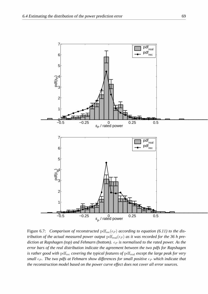
6.4 Estimating the distribution of the power prediction error 69
−0.5 −0.25 0 0.25 0.50
1
2
3
4
5
6
7
εP / rated power
(εP)
pdfreal
pdfrec
−0.5 −0.25 0 0.25 0.50
1
2
3
4
5
6
7
εP / rated power
(εP)
pdfreal
pdfrec
Figure 6.7: Comparison of reconstructedpdfrec(εP ) according to equation (6.11) to the dis-tribution of the actual measured power outputpdfreal(εP ) as it was recorded for the 36 h pre-diction at Rapshagen (top) and Fehmarn (bottom).εP is normalised to the rated power. As theerror bars of the real distribution indicate the agreement between the two pdfs for Rapshagenis rather good withpdfrec covering the typical features ofpdfreal except the large peak for verysmall εP . The two pdfs at Fehmarn show differences for small positiveεP which indicate thatthe reconstruction model based on the power curve effect does not cover all error sources.

70 6 Assessment of wind speed dependent prediction error
6.5 Simple modelling of the power prediction error
Under the assumption that the prediction error of the underlying wind speed prediction does notchange much over the range of typical wind speeds as discussed in section 6.3 the accuracy ofthe power forecast at a particular wind speed expressed as standard deviation of the error, sde,can be described rather well with a very simple approach.
For small deviations between predicted and measured wind speed the sde of the power predic-tion is linearised using a Taylor expansion at the predicted wind speedupred which leads to a“conditional” wind speed dependent error estimate given by
σ(εP )|upred=
∣∣∣∣dP
du
∣∣∣∣upred
σ(εu). (6.12)
This equation is very basic in the sense that it takes only the effect of the local derivativedP/du(upred) of the power curve into account and uses the average sde,σ(εu), obtained frompdf(umeas|upred,i) as accuracy for all wind speeds. The approach neglects that deviations be-tween the certified, i.e. theoretical, power curve and the real power curve might occur whichcan have a significant influence on the prediction error. But this source of error can only be elim-inated by using the corresponding measurement data to correct for these systematic deviationswhile equation (6.12) generally models the error amplification effect of the power curve.
In figure 6.8 the error of the power prediction where the corresponding predicted wind speedis confined to intervals of width1 m/s for the two sites Rapshagen and Fehmarn is plottedversus the predicted wind speed. The bars denote the bin-wise standard deviation of the powerprediction error,sde(εP ) = σ(εP )|upred
at a particular wind speed. Again one year of WMEPdata (see chapter 3) has been used. Obviously, the accuracy of the power prediction dependson the predicted wind speed. This is mainly due to the power curve effect as the solid linecalculated from equation (6.12) indicates.
At Rapshagen this simple model describes rather precisely the behaviour of the actual powerprediction error as illustrated in figure 6.8 (top). However, at Fehmarn (figure 6.8 (bottom))this modelling approach does not lead to an accurate description of the prediction uncertainty.At this site the deviations between predicted and measured power output are not completelyexplained by the linear amplification of small wind speed errors according to equation (6.12)due to differences between the certified and the real power curve. But for many sites the modelprovides a rather good estimation of the wind speed dependent power prediction error.
The amplification of the error caused by the local slope of the power curve is clearly detectablein the sde of the power forecast and can be used to model the prediction error depending onthe wind speed. Figure 6.9 demonstrates how this can be implemented in a power predictionsystem likePreviento. The specific uncertainty of each prediction given by equation (6.12) isillustrated by the shaded area around the predicted value. It is calculated by using the derivativeof the certified power curve and theσ(εu) corresponding to each prediction time. Thus, to applyequation (6.12) for prediction purposes historical data is needed to determine the statisticalerror,σ(εu), of the underlying wind speed prediction.
This uncertainty interval provides additional information to the user and enables him to assess

6.5 Simple modelling of the power prediction error 71
0 2 4 6 8 10 12 140
0.1
0.2
0.3
0.4
0.5
wind speed [m/s]
sde
(εP)
/ rat
ed p
ower
sdemeas
sdemodel
0 2 4 6 8 10 12 140
0.1
0.2
0.3
0.4
0.5
wind speed [m/s]
sde
(εP)
/ rat
ed p
ower
sdemeas
sdemodel
Figure 6.8: Standard deviation of bin-wise power prediction error versus wind speed for the36 h prediction at Rapshagen (top) and Fehmarn (bottom). The bars denote the sde betweenpredicted and measured power output conditioned on wind speed intervals of width 1 m/s. Formedium wind speeds up to 12 m/s the forecast error increases. At Rapshagen this behaviour isvery good approximated by the product of the derivative of the power curve and the wind speederror (solid line) according to equation (6.12) while at Fehmarn the simple modelling approachunderestimates the power prediction error for larger wind speeds which is due to effects notcovered by this model.

72 6 Assessment of wind speed dependent prediction error
toy [d]
pow
er /
rate
d po
wer
10 12 14 16 18 20 22 24 26 280
0.1
0.2
0.3
0.4
0.5
0.6
0.7
0.8
0.9
1uncertaintypredictionmeasurement
Figure 6.9: Times series of prediction (“o”) and measurement (solid line) over a period of18 days. The shaded area is the uncertainty estimate given by equation (6.12). Typically, theuncertainty interval around the predicted value is small for low predictions, i.e. flat slope ofthe power curve, and large for predictions between 20% to 80% of the rated power where thepower curve is steep. Of course, for power outputs near the rated power (not shown here) theuncertainty again decreases.
the risk of a wrong prediction. Of course, this procedure has to be refined in the future by takingthe unsymmetric pdfs of the power error into account (see section 6.4).
6.6 Conclusion
This chapter contains a first approach towards a situation dependent assessment of the predictionerror where wind speed is the indicator that characterises the forecast situation.
Using wind speed as additional parameter a detailed analysis of the statistical properties of theprediction error shows that the conditional probability distribution functions (pdf) of the windspeed error are mainly Gaussian in the range of wind speeds that is important for wind powerapplications. The mean values of these pdfs are as expected on the line given by linear regres-sion of the scatter plot reflecting the systematic error in the prediction. The more interestingquestion whether the prediction error expressed as standard deviation around these mean valuesincreases with increasing wind speed cannot finally be answered here as the data for the differ-ent sites and prediction times does not show a consistent behaviour. However, the results of thischapter suggest that there is only a weak, if any, systematic dependence of the prediction errormeasured as the standard deviation of the differences between prediction and measurement onthe magnitude of the wind speed.

6.6 Conclusion 73
A main result of this chapter is that the non-Gaussian distribution of the power prediction errorcan be modelled. Understanding the mechanism that transforms initially Gaussian wind speederror distributions into strongly non-Gaussian power error distributions allows to easily estimatethe pdf of the power prediction error for any wind farm without knowing the actual predictionsand measurements of the power output.
The approximated reconstruction of the pdf of the power forecast is based on three ingredients:the pdf of the measured wind speed conditioned on the predicted wind speed, the frequencydistribution of the wind speed prediction and the power curve of the wind turbine. However, iffor practical purposes the conditional pdf of the wind speed at a site is not available it can beestimated by assuming that the distribution is Gaussian with a standard deviation of the windspeed error taken from a nearby site or from the publications of the Weather Service (e.g. [55]).The exact frequency distribution of the predicted wind speed could be replaced by either thedistribution of the measurements or distributions from nearby synoptic stations. This means thatan estimate of the statistical distribution of the power prediction error at a site can be obtainedusing information that is readily available for existing wind farms and can even be obtainedprior to the erection of the wind farm at the desired location. This is, for example, convenientto assess the prediction error for future offshore wind farms.
Of course, the “real” distributions of the power prediction errors given by comparing predictedand measured power output might look different. The method derived here does only considerthe effect of the power curve neglecting other sources of error. In particular, the power outputis modelled by plugging wind speeds into the certified power curve representing the averagebehaviour of the wind turbine under standard conditions. However, experience shows that theoutput of individual turbines can well deviate significantly from their certified power curvesfor various reasons [42]. Thus, for practical use the limitation of this reconstruction is clearlythat it is oblivious to these additional error sources beyond wind speed. Nevertheless, it shedssome light on the mechanism that produces the typical non-Gaussian distributions of the powerprediction error.
A very simple model that describes the dependence of the power prediction error on the windspeed with a linearised approach is used. It shows that most of the error can be explained by theinfluence of the power curve that amplifies the rather constant prediction error of the wind speedaccording to its local derivative. This procedure can directly be implemented intoPrevientotoprovide situation dependent uncertainty estimates for each prediction time.
These uncertainty intervals are symmetric which is a major shortcoming of this simple modelbecause it is already clear that the distributions of the power prediction error are non-Gaussianand unsymmetric. However, to provide good estimations of the conditional power distributionsaround each prediction value a lot information has to be recorded concerning the statistics ofthe specific site. Therefore, the simple model suggested here is only the first step towards acomprehensive description of the situation based error statistics.
Parts of the results in this chapter have been published in [35, 33].

74 6 Assessment of wind speed dependent prediction error

7 Relating the forecast error to meteorological situations
Abstract
The investigation in this chapter focuses on the quantitative relation between the error of the wind speed
prediction and the corresponding specific meteorological situation. With methods from synoptic cli-
matology an automatic classification scheme is established using measurements of wind speed, wind
direction and pressure at mean sea level to characterise the local weather conditions at a site. The clas-
sification procedure involvesprincipal component analysisto efficiently reduce the data to the most
relevant modes.Cluster analysisis used to group days with similar meteorological conditions into com-
mon classes. A comparison of these clusters with large-scale weather maps shows that typical weather
situations are successfully captured by the classification scheme. The mean forecast error of the wind
speed prediction of the German Weather Service is calculated for each of the clusters. It is found that
different meteorological situations have indeed significant differences in the prediction error measured
by a daily rmse where the maximum rmse can be by a factor of 1.5 to 1.7 larger than the minimum rmse.
As expected, high uncertainties in the forecast are found in situations where rather dynamic low pressure
systems with fronts cross the area of interest while stationary high pressure situations have significantly
smaller prediction errors.
7.1 Introduction
The investigation in this chapter continues to follow the idea of evaluating the forecast error forspecific weather situations. But in contrast to the previous chapter the meteorological conditionswill now be described by a far larger set of variables than only wind speed to include moredetails of the atmospheric state and its temporal evolution over one day. The aim is to reallydistinguish different weather classes and relate them quantitatively to their typical predictionerrors.
It is a well-known fact that the performance of numerical weather prediction (NWP) systemsis not equally well for every meteorological situation and that their accuracy depends on thesituation that is to be forecast. In an overview of the prediction uncertainty of weather andclimate forecasts Palmer [49] points out that “certain types of atmospheric flow are known tobe rather stable and hence predictable, others to be unstable and unpredictable”. Thus, thechallenge is to know in advance how predictable the current meteorological situation is.
There are already different approaches how to include information about the changing reliabilityof the numerical forecast into the prediction. A very popular one is the use of ensemble predic-tions where the chaotic properties of the non-linear equations of motion of the meteorologicalvariables are exploited, e.g. described in [49, 23]. Lorenz [37] demonstrated that low dimen-sional non-linear weather models are sensitive to small changes in the initial conditions which isthe typical indication of deterministic chaos. Hence, to get an overview over the possible range

76 7 Relating the forecast error to meteorological situations
of weather situations that can evolve from a given situation the initial condition of the NWP isperturbed. Then the NWP calculates separate predictions for each initial condition leading to anensemble of possible outcomes. Thus, ensemble forecasts provide a range of possible weathersituations that can occur with a certain probability. The difficult part is to generate suitableensembles allowing for a statistical interpretation of the results which might differ profoundly.
Ensemble forecasts are computationally expensive and, therefore, for operational use mainlygenerated by large meteorological institutes such as the European Centre for Medium RangeWeather Forecasts (ECMWF). However, Landberg et al. [31] used a simpler version of ensem-ble predictions in connection with wind power application which they denoted as “poor man’sensemble forecast”. The idea is to take the spread between different prediction runs, e.g. at00 UTC and 12 UTC, calculated for the same points of time in the future. The larger the de-viation between the prediction runs the greater the uncertainty of the prediction. This concepthas recently been enhanced by Pinson and Kariniotakis [50]. They established a continuousrisk index from the spread of several forecast runs of the wind speed prediction to derive thecorresponding degree of uncertainty connected to the power prediction.
The technique used in this chapter to assess the uncertainty of a specific prediction is differentfrom the ensemble approach as it is based on a classification scheme of the weather situationwhich is not directly related to the prediction system. The approach here is to describe thesituation of each day by a suitable set of local meteorological variables, then sort it into acertain category, and associate each of the categories with a typical prediction error derivedfrom historical data.
Intuitively, at least two types of meteorological situations over Northern Europe are expected toshow considerable differences in terms of the accuracy of the wind speed prediction. Weathersituations with strong low pressure systems coming in from the Atlantic Ocean are supposedto be of the unstable type that is hard to predict. These situations can be very dynamic as theadvection speed of the low is typically rather large and, in addition, its frontal zones may causestrong winds. In dynamic cases the real situation can evolve quite differently from the onethat had been predicted. In contrast to this high pressure systems with typically moderate windspeeds are rather stationary and can persist for several days which should make it easier for theNWP to provide a reliable prediction.
It is the purpose of this chapter to establish a method that automatically generates useful weatherclasses and, hence, implicitly defines what a “strong low” or a “stationary high” is in terms of thelocal conditions at different sites. Moreover, the investigation here aims to answer the questionhow large the various prediction errors are and whether they differ significantly for differentmeteorological conditions.
7.2 Methods from synoptic climatology
The techniques that are applied in this investigation are well established in synoptic climatology.In a very good overview over the subject Yarnal [65] points out that “synoptic climatology re-lates the atmospheric circulation to the surface environment”. Hence, this branch of climatologyexplicitly aims at linking meteorological conditions to external variables, such as concentration

7.2 Methods from synoptic climatology 77
of air pollutants, which is exactly the type of problem that is addressed in this work.
Quite a variety of powerful methods has been developed in this field and tested in numerousapplications [4, 65, 56]. The main principles are very similar. The first step is to identifytypical structures or patterns of the atmospheric circulation in order to develop a classificationscheme that is only based on meteorological variables. After the classification is establishedthe statistical or deterministic relationship between these structures and a surface variable ofinterest is investigated. Normally, this variable is non-meteorological in the sense that it doesnot describe the state of the atmospheric flow.
Regarding the classification scheme there are two main approaches. On the one hand manualmethods where a meteorologist evaluates the synoptic situation within a certain framework ac-cording to his experience and on the other hand automatic schemes which use computer-basedalgorithms to sort meteorological data into different classes. A well-known manual classifi-cation scheme for Central Europe is the catalogue of “Grosswetterlagen” by Hess and Brez-sowski [19]. It comprises 29 large scale weather situations which are distinguished by theirdifferent spatial arrangement of the pressure systems. In contrast to this, automatic schemestypically exploit correlations between patterns or use eigenvector techniques such as principalcomponent analysis (PCA) to extract synoptic weather classes from numerical data. Yarnal [65]points out that both the manual and the automatic methods contain a certain degree of humansubjectivity because someone has to decide, e.g., on the set of variables and the number ofclasses.
The method chosen in this work to analyse how the forecast error is related to the weathertype relies on computer-based classification techniques and follows in principle an investigationcarried out by Shahgedanova et al. [56]. They used principal component analysis in combina-tion with cluster analysis of surface and upper air meteorological data to derive a classificationscheme of the synoptic situation in Moscow where PCA was used for data reduction and clusteranalysis to sort similar days into common groups. These weather types were then connected totypical concentrations of air pollutants such as CO and NO2. It was found that certain weatherpatterns result in significantly high levels of urban air pollution.
In contrast to Shahgedanova et al. the set of meteorological variables used here will be smallerwith no upper air data involved. The role of the pollutant will be played by the forecast error.In the following the use of PCA and cluster analysis is explained.
7.2.1 Principal component analysis (PCA)
Principal component analysis (PCA) is used to extract the relevant eigenmodes from the me-teorological data. This technique produces eigenmodes which can be ordered according to thedegree of variance they explain in the data. Hence, the modes that contribute most to the timeseries can be selected for the further analysis which allows to effectively reduce the amountof data. The weather situation of each day can then be approximately expressed as a linearcombination of these eigenmodes.
The variables used here are the horizontal wind vector~u = (u, v) and the atmospheric pressureat mean sea level (pmsl). These are the natural candidates to start with as they are closely related

78 7 Relating the forecast error to meteorological situations
to the wind field. To account for temporal variations over one day the variables are taken at 0, 6,12, 18, 24 UTC. Several values of the wind vector per day resolve changes in wind direction andspeed, e.g. during the passage of a frontal system. This provides the possibility of separatingdynamic from static weather situations. The record of the temporal variations of pmsl can partlycompensate for the fact that spatial pressure gradients which are the main driving force of thewind are not available in this investigation.
The temperature that is often included to find synoptic indices is not considered here. This isdone because absolute temperature is mainly used to determine the type of air mass, e.g. byShahgedanova et al. [56], but it is not directly related to the wind field. Moreover, temperaturetends to be a dominating variable that requires the data sets to be split into winter and summerpart. But doing so would leave only half the data points for the analysis which makes it difficultto have significant results in the end. However, for further investigations it would be desirable toinclude temperature and humidity to be able to detect fronts with more parameters than changesin the wind vector. Of particular interest for further investigations are, of course, temperaturedifferences at different heights to assess atmospheric stratification (c.f. Focken [14]).
The measured data are written into a matrixM where the columns contain the different vari-ables and each row corresponds to one day. The measurements at the various day times areconsidered as separate variables. As wind vector and surface pressure have very different or-ders of magnitude both are normalised with their standard deviation and pmsl is additionallycentralised by subtracting the mean value. Hence,M is given by:
M =
u1,0 · · · u1,24 v1,0 · · · v1,24 pmsl1,0 · · · pmsl1,24...
...u365,0 · · · u365,24 v365,0 · · · v365,24 pmsl365,0 · · · pmsl365,24
(7.1)
where the subscripts denote the day of the year and the day time.M is the so-called data matrixwith dimension 365 by 15 having one row for each day of the year with 15 measurements perday at the times 0 h, 6 h, 12 h, 18 h and 24 h UTC.
The PCA of matrixM is carried out numerically by diagonalising the so-called covariancematrixC = M tM . The 15 eigenvectors,~pi, of C are the desired principal components (PC) ofM while the eigenvalues,λi, of C are the weightsλi of the different components that expressthe degree of variance a particular PC contains. A full description of this procedure can befound in Broomhead and King [9].
The set of principal components{~pi} with i = 1, . . . , 15 constitutes a new orthonormal basisof the phase space of the full set of data points. The ordering of the PC according to theeigenvalues,λi, allows to select only the first few PC spanning the subspace where most ofthe relevant dynamics takes place. The number of relevant modes,N , to be considered forfurther analysis is not precisely defined and has to be inferred from the spectrum of eigenvaluesand the corresponding PC. In this investigation the visual inspection of these quantities andthe cumulative variance
∑λi of the firstN eigenvalues will be used as criteria to decide on
the number of modes to be used. Hence, by transforming to new coordinates and reducing

7.2 Methods from synoptic climatology 79
the degrees of freedom PCA efficiently codes the information contained in the meteorologicalraw-data and in that sense acts as a data reduction technique.
The use of PCA as a data reduction technique means that the eigenvalue spectrum is mainlyused to account for the degree of variance contained in each of the corresponding eigenmodes.This is a statistical or climatological interpretation of the eigenspectrum and not a non-linearsystems approach. In the context of dynamic systems a similar technique, time-delay embed-ding, is also applied as a tool to decompose phase space dynamics in different modes with theaim of extracting the degrees of freedom of the non-linear system, e.g. described in detail byBroomhead and King [9] or Kantz and Schreiber [27]. However, the approach used in this workand in particular the construction of the data matrixM does not aim at providing a delay em-bedding of the time series as the sampling intervals are not adapted for this purpose and thenumber of data points is far too low. Hence, the number of eigenmodes provided in this contextcannot contribute to the question how many degrees of freedom the weather or climate systemhas as discussed, e.g., by Nicholis and Nicholis [45] and Grassberger [21].
After a choice concerning the number of relevant PC is made, the data inM is transformed tothe reduced basis such that each day can be represented as a linear combination of the selectedPC. Let{~qi}, i = 1, . . . , N , be the basis chosen from the firstN PC of the full eigenvector basis,{~pi}, of M . Then
Q := (~q1 . . . ~qN) (7.2)
is the transformation matrix that can be used to easily project the data inM on the new basis bya multiplication from the right
X := MQ. (7.3)
The entries inX are the scalar productsxij = ~mi · ~qj where~mi is the i-th row ofM . In otherwordsxij is the contribution of the j-th PC to the i-th day. Consequently, each day~mi can beapproximately (because only aN -dimensional subspace is considered) expressed by
~mi ≈N∑
j=1
xij~qj. (7.4)
Thus, the 365 byN matrix X is the reduced data matrix that is thought to contain most ofthe relevant meteorological information of one year of data. However, so far nothing reallyhappened in terms of the classification scheme because the data has merely been recoded. Thenext step applied to the reduced data set will be cluster analysis.
7.2.2 Cluster analysis
Cluster analysis is a standard method used to group objects with similar properties together. Asdescribed in a concise overview by Everitt [13] it has a wide range of techniques and is oftenapplied in climatological investigations [65, 26, 56].
In this work the aim is to obtain a rather small number of clusters which contain days withsimilar meteorological conditions being different from the days in the other clusters. Of course,the clusters found are required to represent typical weather classes.

80 7 Relating the forecast error to meteorological situations
The type of cluster analysis used here is called hierarchical or agglomerative. It acts iterativelyon the phase space by computing the distances between each pair of objects in the phase spaceand then joining the closest two objects to a new cluster. After the new cluster is formed theprocedure is repeated. Starting point is a situation where all points in the phase space areconsidered as separate clusters. As the final iteration merges all clusters into one group theprocess has to be stopped when a certain number of clusters is reached. The criterion to stopthe iterations is derived from observing the growing distances between the clusters.
Though the basic concept is rather straightforward there are profound differences in the resultsof various clustering procedures because the key point of this technique is how distances be-tween clusters are defined and under which rule new clusters are formed. First of all, a metrichas to be chosen that evaluates distances between single points in the phase space. Here theEuclidean metric (equation (7.5)) is applied as there is no apparent reason for a different one.A more crucial point is the definition of distances between clusters. As the type of distancemeasure implies which two clusters will be joined next it is referred to as “linkage method”.Three typical linkage methods are briefly introduced using the following notations.
Let ~xi := (xi,1, . . . , xi,N) with i = 1, . . . , 365 denote the coordinate vector describing a point intheN dimensional reduced phase space. The distanced(~xi, ~xj) between two states is given bythe Euclidean measure
d(~xi, ~xj) =
√√√√ 1
N
N∑q=1
(xi,q − xj,q)2. (7.5)
After a number ofNA phase states has been joined into one cluster,CA, the members of thiscluster will be denoted as~xA
r wherer = 1, . . . , NA is the new index withinCA.
Complete linkage method
To evaluate the distance between two clustersCA andCB in the complete linkage method allpairs of Euclidian distances between members ofCA andCB are computed. Then the maximumdistance that is found between the individual members is used as distance between the twoclusters. Hence,
dcomplete(CA, CB) := max(d(~xA
r , ~xBp )
)where (~xA
r , ~xBp ) ∈ CA × CB. (7.6)
Average linkage method
Average linkage is a combination of complete linkage as described above and its complementarydefinition, called single linkage, where the minimum of the distance between cluster membersis taken. In average linkage the mean value of the individual distances is used to define thecluster distance between two clustersCA andCB, i.e.
daverage(CA, CB) :=1
NANB
NA∑r=1
NB∑p=1
d(~xAr , ~xB
p ) (7.7)
whereNA andNB are the respective numbers of elements inCA andCB.

7.2 Methods from synoptic climatology 81
Ward’s linkage method
Ward’s method is also referred to as minimum variance method [26] as it evaluates the changeof within-cluster variance if two clusters are merged.
d2ward(CA, CB) :=
NA NB
NA + NB
d(~xA, ~xB
)2
(7.8)
where~xA =∑NA
r=1 ~xAr is the centre of mass of clusterCA and~xB the one ofCB.
Kalkstein et al. [26] thoroughly investigated average linkage, Ward’s linkage and a third tech-nique, centroid linkage, that is not used here. They found that for weather classification pur-poses average linkage produced the “most realistic synoptic groupings” as it provides ratherhomogeneous groups of days with similar meteorological conditions and sorts extreme eventsinto separate clusters instead of combining them into a common class. In contrast to the othertechniques average linkage minimises the within-cluster variance, i.e. the mean variance amongthe days within one cluster, and maximises the between-cluster variance, i.e. the mean variancebetween the centres of mass of different clusters. Shahgedanova et al. [56] also confirmed theusefulness of average linkage in their investigation.
Ward’s linkage on the other hand tends to produce clusters of equal size and, therefore, sortsdays with extreme weather conditions together with less extreme days which “blurs distinctionsbetween the types” [26]. Thus, this method was considered as inferior compared to averagelinkage to produce meaningful synoptic classes. However, Yarnal [65] provides classificationproblems which are quite comparable to those by Kalkstein et al. [26] and Shahgedanova etal.[56] but where Ward’s method is superior to average linkage which leads the conclusion thatboth methods should be tested.
In this work average and Ward’s linkage are used as they have been successfully applied inprevious investigations. Additionally, complete linkage is also applied.
7.2.3 Daily forecast error of wind speed
For the analysis of the forecast error a new error measure is introduced that evaluates the per-formance of the prediction system over one day:
rmseday =
√1
4
∑tpred
(upred,tpred
− umeas,tpred
)2with tpred = 6h, 12h, 18h, 24h (7.9)
whereupred,t andumeas,t are predicted and measured wind speed.
It is, of course, desirable to also include predictions with horizons beyond 24 h into the errormeasure. However, higher lead times have not been included so far because only two largerprediction times, 36 h and 48 h, are available in the investigated data set which is only halfthe number of data points for the analysis compared to the period 6 to 24 h. Hence, this firstapproach is restricted to the earlier lead times.
This “daily error” assigns one single value to each day in a cluster which is analogous to usingthe daily concentration of a pollutant by Shahgedanova et al. [56]. The characteristic property

82 7 Relating the forecast error to meteorological situations
of this definition is that the point of time at which a deviation between prediction and measure-ment occurs is not relevant. Moreover, with the definition in equation (7.9) errors caused bycoherent structures such as a wrongly predicted front are summarised in one error value, i.e. thecorrelation between succeeding deviations is implicitly taken into account.
The idea behind choosingrmseday can be illustrated by an example. Imagine a low pressuresystem approaches the domain of interest. It brings a rise in wind speeds that is predicted forthe late afternoon, say 18 h, but actually arrives a few hours earlier, say 12 h. In this case thedifference between predicted and measured values is rather large and negative at 12 h (becausethe prediction did not foresee the low) and small and negative at 18 h (because the predictionexpected the wind speed to start increasing). Moreover, at 24 h the low has passed and thewind speed actually decreases while the prediction still suggests high wind speeds leading to apositive deviation. Now these situations can typically produce phase errors where the deviationsat a number of lead times in a row are coherently affected. Another important point is that interms of the daily error measure it should not matter whether the low is too fast as in thisexample or is behind schedule, i.e. arrives later than predicted.
7.2.4 Tests of statistical significance
Resolving individual situations reduces the amount of data points available per cluster by abouta factor 10 and, thus, statistical significance becomes an important issue. Therefore, care hasto be taken not to be fooled by statistical artefacts such that in this chapter and the next onetests for statistical relevance will again be applied. To check if the differences in the statisticalvalues of different clusters are not obtained by chance an F-test together with Scheffe’s multiplecomparisons are applied which are based on relating the within-cluster variance of the errorvalues to the variance of the error values in the remaining clusters. The details of the tests aredescribed in the appendix B.

7.3 Results 83
7.3 Results
The methods described above are applied to the data described in chapter 3. To develop a cli-matological classification scheme measured data from one year is used. The horizontal windvector~u at a site is calculated by sine-cosine transformation of the measured wind speed and di-rection at, preferably, 30 m to avoid artefacts from obstacles that might occur for lower heights.However, if the 30 m measurement is not available 10 m data are also used. The correspondingsurface pressure is taken from the nearest synoptic station of the German Weather Service. It isconverted to mean sea level using the barometric height formula.
To avoid complications due to missing data points only sites with a high data availability in windspeed, wind direction and surface pressure are chosen. This requirement limits the number ofsuitable sites compared to the error evaluation in chapter 4. Hence, the investigation here willfocus on four locations (see map 3.1): Fehmarn, Hilkenbrook with 30 m wind data and Syke,Rapshagen with 10 m wind data. Fehmarn is an island in the Baltic Sea close to the Germancoast. The site that is investigated is near the island’s shore line and, hence, exposed to ratherinhomogeneous conditions. Northerly and north westerly winds approach the site over the seawhile easterly to south westerly winds arrive over land. In contrast to this Hilkenbrook is in thenorth western part of Germany about 70 km south of the coast of the North Sea. The terrain isvery homogenous in terms of the surface roughness and no orographic effects are to be expected.Syke is also located about 50 km east of Hilkenbrook in slightly hilly terrain. This also holdsfor Rapshagen which is situated in the east of Germany about 100 km south of the Baltic Sea.
The results are presented in the following way. First the modes extracted from the meteorologi-cal variables with PCA are presented. Then cluster analysis is applied to the reduced data matrixand the typical weather classes that are obtained by a straightforward approach are shown forcomplete as well as Ward’s linkage and compared to large-scale weather maps. The averageforecast error of the wind speed for each cluster is provided and discussed for the differentlinkage techniques.
7.3.1 Extraction of climatological modes
The PCA as described in section 7.2.1 is carried out numerically using routines from the stan-dard software MATLAB. In figure 7.1 the eigenvalues,λi, of the PCA for Fehmarn, Hilkenbrookand Rapshagen are shown. The eigenvalues are normalised with the total variance, i.e. the sumof all eigenvalues. It can be clearly seen in figure 7.1 that the eigenvalues decay rapidly withthe first six eigenvalues already explaining about 90 % of the variance.
The spectra are surprisingly similar though the stations are in regions with distinct weatherregimes and different local conditions around the site. There are only minor deviations for thefirst and most important eigenvalues, i.e. the distribution of variance among the correspondingPC is very consistent. The eigenvalues for Syke are not shown as they are as expected almostidentical to those of the rather adjacent site Hilkenbrook.
The first six principal components (PC) in~u-space of Fehmarn and Hilkenbrook are shownin figure 7.2. The temporal evolution of~u(t) = (ut, vt) at timest = 0, 6, 12, 18 and 24 h isindicated by connecting the end points(ut, vt) with lines. Note that the wind vector, i.e. the

84 7 Relating the forecast error to meteorological situations
1 3 5 7 9 11 13 150
0.1
0.2
0.3
0.4
0.5
index
nor
mal
ized
eig
enva
lue
FehmarnHilkenbrookRapshagen
Figure 7.1: PCA eigenvalue spectrum normalised by sum of the eigenvalues, i.e. the total vari-ance, for three sites (Fehmarn, Hilkenbrook and Rapshagen). Though the sites have differentlocal wind characteristics the spectra are very similar.
direction in which the wind blows, is shown while the description of wind directions will referto the direction from which the wind comes. Hence, e.g. southerly winds refer to wind vectorspointing to the north.
The corresponding PC of pmsl are illustrated in figure 7.3. Note that the PC do not necessarilycorrespond to actual meteorological conditions at the location on a specific day. They constitutethe set of vectors whose linear combination can approximately reconstruct the current situation(cf. equation (7.4)).
Typically, the first two PC are rather stationary in that they show little diurnal variation in termsof wind direction and pressure. For all investigated sites the first PC describes moderate windspeeds from east or north east with slightly higher wind speeds at noon and virtually no changein wind direction over the day (see figs. 7.2 and 7.3). In addition, the pmsl is at a constantlyhigh level. PC 2 is also very consistent for different locations. It refers to north westerly winddirections with increasing wind speeds at midday. The corresponding pmsl is slightly rising at ahigh level. In terms of~u these first two PC can roughly be associated with the two most frequentflow directions at the site.
The third PC is again similar for all sites although it occurs with different signs. As the sign ofthe PC is arbitrary, those PC which only differ in their sign are regarded as identical climatolog-ical modes. In half of the cases PC 3 refers to wind from the north with pmsl increasing fromlow to medium level while for the other half it describes wind from the south in connection withpmsl falling from high to medium level.

7.3 Results 85
Higher principal components are much more dynamic for all sites than the first three PC. As canbe seen in figs.7.2 and 7.3 the diurnal variations in all variables are profound. PC 4 to 6 typicallyrefer to changes in wind direction of about 180 deg up to 300 deg with rapidly changing windspeeds and pmsl. Hence, these PC are needed to account for changing meteorological conditionsover one day.
For adjacent stations the PC are almost identical. However, even for sites that are supposedto be located in different climatological conditions like Fehmarn and Hilkenbrook the sets ofrelevant PC are surprisingly similar. This suggests that PCA extracts fundamental modes of theclimatology that are quite universal for the investigated area of northern Germany.
The inspection of the eigenvalue spectra in figure 7.1 reveals that the first four PC on averagecontribute most to the meteorological signal. However, the structure of the PC as discussedabove showed that, in particular, the PC 4 to 6 describe the dynamic changes of the weathercondition occurring within 24 hours. Hence, these higher modes are expected to represent moreextreme meteorological situations which do not occur very often but are supposed to accountfor larger forecast errors than more stationary modes. Consequently, the first six PC are chosen,i.e.N = 6, as the orthogonal basis{~qi}, i = 1, . . . , 6, spanning the reduced state space.
Hence, the number of modes chosen here is slightly larger compared to what the eigenspectrumsuggests. Yarnal [65] points out that the use of too many eigenmodes does not necessarilyenhance the performance of the following cluster analysis which is quite understandable as theadditional variation introduced by including more modes might not contain useful informationbut mainly noise. However, in the course of this investigation it will turn out that in particularthe PC which describe changes in the meteorological variables over one day are important. Theuse of less than six PC has so far not been investigated.
According to equations (7.2) and (7.3) the data matrixM is projected onto the new basis andthe day-score matrixX is obtained that contains the contributions of the six PC to the meteoro-logical situation of a specific day.

86 7 Relating the forecast error to meteorological situations
−0.5 0 0.5
−0.5
0
0.5
u [arb. units]
v [a
rb. u
nits
]PC 1PC 2PC 3PC 4PC 5PC 6
−0.5 0 0.5
−0.5
0
0.5
u [arb. units]
v [a
rb. u
nits
]
PC 1PC 2PC 3PC 4PC 5PC 6
Figure 7.2: First six principal components (PC) of~u space for Fehmarn (top) and Hilkenbrook(bottom). The symbols denote the points(ut, vt) at timest=0, 6, 12, 18, 24 h where(u0, v0)
(t=0 h) is marked by “+”. The first three PC are stationary with slight wind speed variationsover the day. The higher PC describe changes in the meteorological situation.

7.3 Results 87
0 6 12 18 24
−0.5
0
0.5
hour of day
pm
sl [a
rb. u
nits
]
PC 1PC 2PC 3PC 4PC 5PC 6
0 6 12 18 24
−0.5
0
0.5
hour of day
pm
sl [a
rb. u
nits
]
PC 1PC 2PC 3PC 4PC 5PC 6
Figure 7.3: First six PC of pmsl space for Fehmarn (top) and Hilkenbrook (bottom). The firsttwo PC refer to rather constant high pressure while the higher PC describe changes in pmslwhich can be rather dramatic, e.g. PC 6.

88 7 Relating the forecast error to meteorological situations
7.3.2 Meteorological situations and their forecast error
The 365 by 6 day-score matrixX is the basic element of the cluster analysis as its rows con-stitute the phase space points that are to be grouped together. The three linkage techniquesaverage, complete and Ward’s linkage have been used in this investigation to define clusters. Incontrast to Shagedanova et al. [56] and Kalkstein et al. [26] average linkage as defined in equa-tion (7.7) failed in producing meaningful synoptic classes as it sorted two thirds of the daysinto one common group and divided the remaining days into a number of very small groups.Complete linkage (equation (7.6)) and Ward’s linkage (equation (7.8)) produce clusters that canbe associated with typical weather situations and, hence, the classification schemes based onthese linkage types appear to be reasonable. In the following the results of complete and Ward’slinkage are presented for the two sites Fehmarn and Hilkenbrook.
Complete linkage
The first step of the cluster analysis is to successively join the objects in the phase space startingfrom 365 separate days up to one single cluster and record the distances according to equa-tion (7.6) of the two clusters that have been formed in each step. The larger the distance thegreater the difference between the clusters in terms of the chosen linkage method. Hence, theclustering process should be interrupted if the distances between the clusters become too largewhich is often indicated by a “jump” in the series of distances.
Figures 7.4 and 7.5 show the distances of the final 15 clustering steps using complete linkage atthe two sites. In both cases there are several jumps in the distances that suggest the unificationof two clusters that are quite distinct. For Fehmarn two crucial points can be identified at thetransition from seven to six and from five to four clusters. At Hilkenbrook detectable steps inthe cluster distances occur at the transition from eight to seven and also five to four clusters.
In this investigation it turns out that the classification scheme is quite robust in the sense thatuseful classification results can be obtained for different cluster numbers. The behaviour ofthe cluster distances suggests a range of possible cluster numbers that should be consideredfor further investigations rather than providing just one optimal number. Which number ofclusters is selected depends on the detailed purpose of the investigation. In order to interpreteclusters in terms of weather classes and to compare clusters found at different sites it is useful tochoose a number of six to eight clusters because the synoptic situations are more homogeneous.However, using more clusters means that a smaller proportion of the 365 days per year aregrouped together in a common cluster. This can lead to less significant results with regard tothe average forecast error. As a consequence, it seems advisable to vary the number of clustersin the range indicated by the discontinuities in the cluster distances and to carefully considerthe results in terms of the corresponding weather class on the one hand and the forecast erroron the other hand. As the clustering technique has the very convenient property that only twoclusters are joined at each step without affecting the remaining groups it is easy two follow whatactually happens if the number of clusters is varied.

7.3 Results 89
0 1 2 3 4 5 6 7 8 9 10 11 12 13 14 155
6
7
8
9
10
11
12
13
14
15
16
number of clusters
clu
ster
dis
tanc
e [a
rb. u
nits
]
Figure 7.4: Distance between clusters using complete linkage at Fehmarn. As clusters aresuccessively joined “jumps” in the distances start to occur at the transitions from seven tosix and five to four clusters. This defines the range of cluster numbers considered for furtheranalysis.
0 1 2 3 4 5 6 7 8 9 10 11 12 13 14 155
6
7
8
9
10
11
12
13
14
15
16
number of clusters
clu
ster
dis
tanc
e [a
rb. u
nits
]
Figure 7.5: Distance between clusters using complete linkage at Hilkenbrook. The discontinu-ities at the transitions from eight to seven and five to four.

90 7 Relating the forecast error to meteorological situations
Complete linkage at Fehmarn
Following this approach six clusters are used for Fehmarn to see how they can be connected tothe overall weather situation. After the clusters are defined the corresponding meteorologicalsituation is considered in terms of the mean values of “real”~u and pmsl for each cluster. Fig-ure 7.6 shows the mean values of the meteorological variables of Fehmarn’s six clusters. Notethat~u denotes the wind vector and points in the direction in which the wind blows whereas winddirections, as usual in meteorology, refer to the direction from which the wind blows. In termsof pmsl (fig.7.6 (bottom)) the clusters show three different regimes: low pressure (clusters 1, 2and 5), moderately high pmsl (clusters 3 and 6) and very high pmsl (cluster 4).
The low pressure situations differ considerably with respect to wind speed and direction (fig.7.6(top)). Typically, cluster 1 has moderate winds from south west and slightly decreasing pressurecaused by a low pressure system approaching from the west or north west together with a highsouth of the site. The large-scale weather map of a typical day of cluster 1 is shown in figure 7.7(top). Cluster 2 refers to a strong low that passes north of the site as illustrated in figure 7.7(middle). The pmsl drops on average to a low level around 1000 mbar and recovers again at theend of the day. The wind speeds are very high with wind direction changing from south westto west north west and then back to south west. Cluster 5 is related to a situation where the lowpasses west of the site, e.g.over Britain and France, with high pressure gradients over the BalticSea (figure 7.7 (bottom)). Wind speeds are quite considerable turning from south east to northeast.
The two clusters with moderately high pmsl around 1020 mbar correspond to different flowsituations. Cluster 3 is related to moderate wind speeds from easterly directions. This typicallyoccurs if a stable high pressure area persists over western Russia and a rather strong low islocated west of the site leading to considerable pressure gradients over Fehmarn (figure 7.8(top)). Days in cluster 6 are characterised by almost the same mean pressure as cluster 3 butwith north westerly wind directions. In this case central Europe is influenced by a high or ridgelocated west or north west of the site (figure 7.8 (middle)).
Cluster 4 summarises mainly days from the winter period with very high pmsl around 1030 mbarand easterly winds. The corresponding weather situation is typically associated with high pres-sure over Scandinavia extending over Central Europe as shown in figure 7.8 (bottom).
Comparing the large-scale weather maps of days within one cluster shows that the overallweather situation for most of the days is rather coherent. Hence, the classification schemethat is based on local data at the site can be related to the overall weather situation. This is nottotally surprising as the local meteorological situation described by wind speed, direction andpressure is caused by the atmospheric circulation on a larger scale. Of course, for some days theweather situations are not very precisely described by the mean values of the cluster. If moreclasses are used clusters typically split into new clusters which are in itself more homogeneousthan before. But with regard to the investigation in this work a small number of clusters isdesired and sufficient even though the division might be too rough for other purposes. On thewhole, the synoptic classification using six clusters with complete linkage for Fehmarn appearsto be reasonable.

7.3 Results 91
−10 −5 0 5 10
−10
−5
0
5
10
u [m/s]
v [m
/s]
cluster 1cluster 2cluster 3cluster 4cluster 5cluster 6
hour of day
pm
sl [m
bar]
0 6 12 18 24975
980
985
990
995
1000
1005
1010
1015
1020
1025
1030
1035
cluster 1cluster 2cluster 3cluster 4cluster 5cluster 6
Figure 7.6: Means of~u (top) and pmsl (bottom) for six clusters at Fehmarn constructed withcomplete linkage. For~u the symbols denote the points(ut, vt) at timest=0, 6, 12, 18, 24 hwhere(u0, v0) (t=0 h) is marked by “+”. The corresponding weather situations are shown infigures 7.7 and 7.8.

92 7 Relating the forecast error to meteorological situations
Figure 7.7: Large-scale Weather maps of days inside a specific cluster representing typicalweather classes derived by complete linkage at Fehmarn located at 54 deg N, 12 deg E. Top:Low pressure approaching from North West (cluster 1). Middle: Strong low passes north ofGermany (cluster 2). Bottom: Low passing west of Fehmarn over Britain and France (cluster 5).

7.3 Results 93
Figure 7.8: Same as figure 7.7 but for different weather classes. Top: Stationary high pressureover western Russia (cluster 3). Middle: High pressure area north west of Germany with lowover western Russia (cluster 6). Bottom: Strong high pressure system over Scandinavia withlow influencing west of Europe (cluster 4).

94 7 Relating the forecast error to meteorological situations
Complete linkage at Hilkenbrook
Hilkenbrook is about 250 km west of Fehmarn and, therefore, expected to be exposed to dif-ferent wind conditions, in particular, less influenced by continental high pressure systems overScandinavia and Russia but more affected by lows approaching from the Atlantic Ocean. How-ever, there should be a number of weather situations which are comparable to Fehmarn as thesize of the overall circulation patters is much larger than the distance between the sites. This isconfirmed by considering the means of the meteorological variables in the seven clusters cre-ated by complete linkage for Hilkenbrook in figure 7.9. Again the clusters are roughly orderedaccording to low pressure (clusters 5 and 6), moderate pmsl (clusters 3 and 4), and high pmsl(clusters 1, 2 and 7).
The two low pressure classes both refer to rather dynamic situations with pmsl varying over theday (figure 7.9). Cluster 5 has high wind speeds from the south with pmsl dropping from about1005 mbar to 995 mbar due to a low pressure system approaching from the north or north west.Cluster 6 is related to a strong low passing north of the site. The wind blows rather strongly andturns from south west to west and back to south west indicating the passage of a front.
Moderate pmsl around 1010 mbar occurs at Hilkenbrook mainly in two different weatherregimes. Cluster 3 shows rather high wind speeds from the east and slightly increasing pressuretypically related to a high pressure system east or north east of the site, e.g.over western Russia,and low pressure in the west or south west. Cluster 4 contains quite a number of days whichhave pmsl around 1010 mbar and very low wind speeds. The weather class is not as clear as inall the other clusters but mainly characterised by the fact that the centres of the pressure areasare far away with small pressure gradients at the location of the site.
The three high pressure clusters at Hilkenbrook show quite pronounced differences concerningtheir mean wind directions. Cluster 1 has on average the highest pmsl of about 1023 mbar.Note that this is more than 5 mbar lower compared to the highest pmsl at Fehmarn. The winddirections are from the east with moderate speeds. The overall weather situation is typicallydominated by a stationary high pressure system over Scandinavia and, hence, north east of thesite. In contrast to this, cluster 2 refers to a weather situation where the high pressure area islocated in the west of the site leading to northerly wind directions. Finally, cluster 7 is relatedto south westerly winds caused by high pressure south west or south of the site and at the sametime low pressure in the north.
Hence, also for Hilkenbrook the classification of meteorological situations based on completelinkage appears to be useful.
The typical weather classes found for the two sites seem to be rather similar in terms of thegeneral description of the meteorological situations. In order to further test the consistencyof the classification scheme the days that simultaneously appear in clusters from Fehmarn andHilkenbrook are counted. The result is shown in table 7.1 where the rows refer to Fehmarn’sclusters and the columns to those from Hilkenbrook.
Some clusters share a rather profound number of days. For example, cluster 2 of Fehmarn is,except of two days, completely contained in Hilkenbrook’s cluster 6. Hence, on these 15 daysthe classification at both sites records a weather situation dominated by a strong low pressure

7.3 Results 95
−10 −5 0 5 10
−10
−5
0
5
10
u [m/s]
v [m
/s]
cluster 1cluster 2cluster 3cluster 4cluster 5cluster 6cluster 7
hour of day
pm
sl [m
bar]
0 6 12 18 24975
980
985
990
995
1000
1005
1010
1015
1020
1025
1030
1035
cluster 1cluster 2cluster 3cluster 4cluster 5cluster 6cluster 7
Figure 7.9: Means of~u (top) and pmsl (bottom) for seven clusters found for Hilkenbrook withcomplete linkage. For~u the symbols denote the points(ut, vt) at timest=0, 6, 12, 18, 24 hwhere(u0, v0) (t=0 h) is marked by “+”.

96 7 Relating the forecast error to meteorological situations
Table 7.1: Comparison of equal days in clusters for Fehmarn and Hilkenbrook.
Hilkenbrookcluster 1 cluster 2 cluster 3 cluster 4 cluster 5 cluster 6 cluster 7
∑Fehmarncluster 1 0 0 0 29 12 6 3 50cluster 2 0 0 0 0 0 15 2 17cluster 3 30 16 15 51 2 0 7 121cluster 4 35 0 0 0 0 0 0 35cluster 5 0 0 3 16 1 1 0 21cluster 6 4 43 0 38 0 0 36 121
∑69 59 18 134 15 22 48 365
system that is centred north of Germany and moves quickly to the north east. However, the exactpath and the advection time of the low decides whether both sites are affected simultaneouslyor only one of them. If the low takes a more southern route only Hilkenbrook classifies thissituation as cluster 6 while Fehmarn has a smaller pressure drop and lower wind speeds as it islocated further in the east and, hence, might not to affected by the fronts. Fehmarn labels thissituation as cluster 1.
Another example is cluster 4 of Fehmarn which is totally absorbed by cluster 1 of Hilkenbrook.These 35 days are typically related to a high pressure system over Scandinavia or WesternRussia with extremely high pmsl over north eastern Germany. However, Hilkenbrook’s cluster 1contains more days than that which overlap with cluster 3 of Fehmarn. At these days the highpressure system is located further in the east leading to similar wind directions from the eastand pmsl around 1020 mbar at both sites.
On the other hand, certain weather situations lead to very different classification results at bothstations, e.g. cluster 3 of Fehmarn is distributed over six different clusters of Hilkenbrook. Thisoccurs if the two sites are influenced by distinct weather regimes. In this case Fehmarn is dom-inated by rather high pressure located over western Russia while at the same time Hilkenbrookcan experience a variety of high or lower pressure situations.
The result of this comparison is that the consistency between the classifications at the two sitesseems to be very high. For the majority of cases common days in clusters can be plausiblyexplained by the overall weather situation that either shows that the two sites are affected in thesame way or why they simultaneously record different local conditions.
Relation to forecast error using complete linkage
For each of the clusters the mean forecast error is determined by averaging the rmse valuescalculated for each day with equation (7.9). As described in chapter 3 the wind speed predictionat 10 m is provided by the “Deutschlandmodell” of the German Weather Service while thecorresponding wind speed measurements are from the WMEP programme. Thus, the errors

7.3 Results 97
are determined based on the same data that has been used in chapter 4 to evaluate the overallperformance of the wind speed forecast.
The means of the daily rmse values per cluster normalised to the annual average of the windspeed are shown in figure 7.10 for Fehmarn and figure 7.11 for Hilkenbrook found with com-plete linkage. In both cases there are considerable differences between the forecast errors of thedifferent clusters. The error bars illustrate the 95% confidence intervals of the mean values sug-gesting that the clusters with minimum and maximum rmse are indeed significantly separated(detailed results of the statistical tests on this matter can be found in appendix B).
cluster no.
rel.
rmse
of w
ind
spee
d pr
edic
tion
1 2 3 4 5 60
0.1
0.2
0.3
0.4
0.5
0.6
Figure 7.10: Means of daily rmse of wind speed prediction normalised with annual mean ofwind speed for the six clusters found with complete linkage at the site Fehmarn. The error barsillustrate the 95% confidence intervals of the mean. Clusters 1, 2 and 5 show the largest error.In both cases the corresponding weather situation is dominated by a low pressure system. Allthree clusters have significantly larger forecast errors than cluster 4 which typically refers to astationary high pressure situation and has a significantly lower rmse compared to clusters 1, 2and 5 (see table B.2).
In particular, Fehmarn’s clusters 1, 2 and 5 are related to very high relative rmse values around0.38 corresponding to about 2.1 m/s absolute rmse. As described before (fig. 7.6) these threeclusters are related to different low pressure situations. Cluster 2 corresponds to situationswhere a strong low passes north of the site and has on average the highest forecast error. Incontrast to this cluster 4 representing the weather type with the largest pressure has the smallestrmse of about 0.23 relative and 1.3 m/s absolute. A statistical F-test (with confidence level 0.05)confirms that this is significantly lower compared to the above mentioned classes 1, 2 and 5 (seetable B.2). The ratio between the largest and the smallest rmse is 1.7 which is very profound.
At Hilkenbrook cluster 6 has the highest rmse with 1.8 m/s absolute and 0.51 relative. Thecorresponding weather situation is related to a low pressure system passing north of the site.The cluster with the smallest average forecast error is cluster 1 related to a rather stationary

98 7 Relating the forecast error to meteorological situations
cluster no.
rel.
rmse
of w
ind
spee
d pr
edic
tion
1 2 3 4 5 6 70
0.1
0.2
0.3
0.4
0.5
0.6
Figure 7.11: Same as figure 7.10 but for the seven clusters found with complete linkage atHilkenbrook. Cluster 6 has the maximum forecast error which is significantly different fromclusters 1, 2, 4 and 7. Cluster 6 is related to a low pressure system passing north of the site.Cluster 1 with the smallest rmse corresponds to a situation where a stationary high pressuredominates the local weather conditions. Its error is significantly lower compared to clusters 4and 6 (see table B.4).
high pressure situation where the rmse is 1.0 m/s absolute and 0.29 relative to the mean windspeed. The ratio between the maximum and minimum rmse is 1.8. It is also interesting to notethat the forecast error in cluster 4 is on a medium level of 0.39 relative rmse (1.4 m/s) whichis roughly half way in between the smallest and largest error values and significantly differentfrom both of them. The days in this cluster are related to medium pmsl with small pressuregradients and, hence, low wind speeds.
Again the average forecast errors found for the typical weather situations at the two sites showa very good consistency. For Fehmarn as well as for Hilkenbrook large rmse values occur forthe clusters that are related to a rather fast moving low pressure system that passes north ofthe site (cluster 2 for Fehmarn, 6 for Hilkenbrook). The local meteorological conditions arecharacterised by pmsl on a very low level further decreasing around midday but recovering atthe end of the day. Wind speeds are fairly high with wind directions turning from south west towest and back to south west indicating the passage of a front. Depending on the path of the lowthis situation simultaneously occurs at both sites or only at Hilkenbrook (see table 7.1).
In addition, for Fehmarn the passage of low pressure areas in the west or south west of the sitewith strong easterly winds (cluster 5) is also related to large forecast errors. At Hilkenbrookthese days are recorded in cluster 4 which additionally contains more situations with on averagesmaller wind speeds and slightly higher pmsl compared to Fehmarn. The corresponding forecasterror is the second largest at Hilkenbrook but significantly lower than the largest one. Thus, atFehmarn there are higher wind speeds caused by larger pressure gradients while at the same

7.3 Results 99
time at Hilkenbrook more moderate conditions prevail.
In contrast to this, both sites have the smallest forecast error in situations where a high pressurearea lies rather stationary over Scandinavia or the Baltic Sea with relatively high wind speedsfrom the east. For Fehmarn the mean rmse in this case is 17% to 39% smaller than those of theother weather classes. For Hilkenbrook the minimum rmse is 13% to 42% smaller than in theother clusters.
Hence, using complete linkage leads to a reasonable synoptic classification of the meteorologi-cal data (30 m wind data and pmsl of nearby synop station) at these two sites in the sense that theclusters can be associated with typical large-scale weather classes. The number of classes foundby considering the interval of clustering steps given by “jumps” in the distances between theclusters as criterion to stop the clustering process already provides a good choice. Moreover, themean forecast errors related to the clusters show significant differences where the maximum andminimum rmse are as expected related to dynamic low pressure and stationary high pressure,respectively.
Ward’s linkage
For most of the investigated sites Ward’s linkage produced clusters which are in principle com-parable to those found by complete linkage. But the alterations between the groups of daysgenerated by the two methods can make important differences in terms of the grouping of daysand, thus, the related forecast errors. This is now illustrated for Fehmarn where typical differ-ences between the methods occur.
As figure 7.12 shows the distances between the clusters at the final 15 steps of the clusteringprocedure behave very similar to complete linkage. There are discontinuities at the transitionsfrom eight to seven and five to four clusters. Again choosing a number of clusters from thisinterval leads to a classification that allows to relate the clusters to large-scale weather situationsand to find significant differences between the average forecast errors per cluster.
The results of the classification based on six clusters with Ward’s linkage for Fehmarn areshown in figures 7.13. With regard to these mean values of~u and pmsl the classes are generallycomparable to those found by complete linkage in figures 7.6. But it is obvious by comparingthe means of the pressure that there are differences in particular for the low to medium rangewith pmsl between 1005 mbar and 1015 mbar. Moreover, in terms of the mean wind vectorsWard’s cluster 1 appears to constitute a new class which does not appear under complete linkage.
A more detailed comparison of the overlaps between the clusters reveals that some days aregrouped rather differently by the two methods. Table 7.2 shows that the only two clusters thatare nearly identical are number 2 of complete and 5 of Ward’s which share 16 common daysrelated to the well-known weather situation of the passing low in the north. Hence, these seldombut rather extreme days are consistently classified by both methods.
Another interesting weather class is the high over Scandinavia or the Baltic Sea detected bycomplete linkage as cluster 4. Under Ward’s linkage these 33 days with very high pressureare almost totally contained in cluster 2. But this cluster contains additional days from situ-ations with slightly lower pmsl and lower wind speeds. Hence, Ward’s cluster 2 joins days

100 7 Relating the forecast error to meteorological situations
0 1 2 3 4 5 6 7 8 9 10 11 125
10
15
20
25
30
35
40
number of clusters
clu
ster
dis
tanc
e [a
rb. u
nits
]
Figure 7.12: Distance between clusters using Ward’s linkage at Fehmarn. “Jumps” in thedistances occur at the transitions from eight to seven and five to four clusters. This is verysimilar to complete linkage (fig.7.4).
into one class that are separately classified under complete linkage, i.e. clusters 3 (pmsl around1020 mbar) and 4 (very high pmsl≈ 1030 mbar). This tendency of Ward’s linkage to groupextreme together with less extreme situations though they should remain distinct has alreadybeen described in earlier investigations, e.g. by Kalkstein et al. [26]. Another typical feature ofWard’s method is to create rather equally sized groups which can also be observed in table 7.2.The distribution of days on the clusters is more balanced compared to complete linkage.
Table 7.2: Comparison of equal days in clusters complete and Ward’s linkage for Fehmarn.Though the means of the clusters are rather similar to complete linkage there are differences inthe actual grouping.
Wardcluster 1 cluster 2 cluster 3 cluster 4 cluster 5 cluster 6
∑Completecluster 1 0 0 30 0 4 16 50cluster 2 0 0 1 0 16 0 17cluster 3 10 24 32 0 0 55 121cluster 4 0 33 0 2 0 0 35cluster 5 0 0 0 0 1 20 21cluster 6 22 0 41 55 3 0 121
∑32 57 104 57 24 91 365

7.3 Results 101
−10 −5 0 5 10
−10
−5
0
5
10
u [m/s]
v [m
/s]
cluster 1cluster 2cluster 3cluster 4cluster 5cluster 6
hour of day
pm
sl [m
bar]
0 6 12 18 24975
980
985
990
995
1000
1005
1010
1015
1020
1025
1030
1035
cluster 1cluster 2cluster 3cluster 4cluster 5cluster 6
Figure 7.13: Means of~u (top) and pmsl (bottom) for six clusters with found by Ward’s linkageat Fehmarn. For~u the symbols denote the points(ut, vt) at timest=0, 6, 12, 18, 24 h where(u0, v0) (t=0 h) is marked by “+”. Some of the clusters are comparable with those provided bycomplete linkage (figure 7.6), in particular cluster 5 with cluster 2 by complete linkage.

102 7 Relating the forecast error to meteorological situations
Relation to forecast error using Ward’s linkage
The mean daily forecast error per cluster for Ward’s linkage is shown in figure 7.14. Comparedto the rmse of the complete linkage clusters in figure 7.10 the differences between the classesare less pronounced. The statistical F-test reveals that cluster 2 with the lowest rmse is signifi-cantly different from clusters 3 and 6 with the highest rmse (c.f. table B.3 in the appendix). Butin contrast to this, complete linkage results in a higher number of significantly different clusters,in particular the cluster with the smallest prediction error has a significantly lower rmse thanthree of the other clusters. Thus, at this site Ward’s clusters have rather equalised error levelswith smaller differences between the clusters. This is considered as a disadvantage compared tocomplete linkage as the classification scheme that provides a better distinction between the fore-cast errors is more useful. Of course, under the condition that it produces rather homogeneousclusters which can be associated with certain weather types.
cluster no.
rel.
rmse
of w
ind
spee
d pr
edic
tion
1 2 3 4 5 60
0.1
0.2
0.3
0.4
0.5
0.6
Figure 7.14: Means of daily rmse for the six clusters found with Ward’s linkage at Fehmarn.The differences between the forecast errors are not as pronounced as for complete linkage (fig-ure 7.10 and table B.3).
For the sites in this investigation the clusters constructed by Ward’s linkage provided a clas-sification scheme that appears to correspond to typical weather situations. But compared tocomplete linkage the grouping of days can be different with a slight trend to join distinct me-teorological situations into common classes and to form equally sized groups. However, incontrast to the findings by Kalkstein et al. [26] Ward’s linkage does not appear “to blur distinc-tions between types”. In terms of the related prediction error complete linkage performs betterthan Ward’s linkage at Fehmarn and Hilkenbrook as it provides sharper distinctions betweenthe clusters.

7.3 Results 103
Results for other sites
The site Syke is about 50 km west of Hilkenbrook still in the north western part of Germany. Theresults based on complete linkage using of measurements of wind data at 10 m height instead of30 m as before are rather similar to Hilkenbrook. Here the passage of the low centred in the northis also related to the maximum forecast error. The minimum rmse also occurs for a high pressuresituation but in contrast to the two sites above the high is west of the site. The Scandinavian highthat leads to the minimum forecast errors for the sites above still has a relatively small rmse.At Syke the performance of Ward’s technique is comparable to the complete method. Thebehaviour of the forecast error for the different weather classes, particularly, the systematicallylarger rmse for dynamic low pressure situations is also confirmed under Ward’s linkage.
At Rapshagen complete linkage (also 10 m wind data) provides clusters whose interpretationin terms of large-scale weather classes is not as clear as for the other sites. At this site Ward’slinkage seems to be superior and leads to a classification that is easier to relate to weather pat-terns. The forecast errors per cluster again show that the well-known low pressure passage hasa rather high rmse but certain high pressure conditions also have. However, this site should betreated with care as local effects seem to strongly influence the flow conditions locally thoughthe orography is only slightly complex. In terms of the relation between meteorological con-ditions and the forecast error this leads to an overlap between the overall predictability of theweather situation by the NWP and local effects on the wind field due to the specific on-siteconditions.
Regarding local effects, e.g.due to orography causing speed up effects over hills and channelingeffects in valleys, it has to be points out that the classification method works with on-site infor-mation and is, therefore, unable to tell local flow distortion from global circulation. Hence, localeffects are implicitly taken into account and there might be an overlap between the two effects.Among the investigated sites only one site (Rapshagen) obviously shows this phenomenom andmakes it difficult to draw definite conclusions while the other sites do not show strong signs oflocal effects in the course of the analysis.
As a summary the results for all investigated sites are given in table 7.3 where the relative rmsefor the three weather classes “low passes in the north”, “Scandinavian high” and “high centredin north west” having the most distinct differences in terms of the forecast error are shown. Therather dynamic passage of the low leads to large prediction errors at all sites with the relativermse ranging from 0.31 to 0.51. Compared to this the two high pressure situations are relatedto significantly smaller forecast errors. The high over Scandinavia causes an average rmse from0.23 to 0.29 with the exception of the very unusual error value of 0.43 at Rapshagen presumablyrelated to orographic effects. A high pressure area centred north west or west of the sites hasalso rather small relative rmse between 0.22 and 0.36. To express the difference between theweather classes in terms of the forecast error the ratio between the maximum rmse of the lowpressure situation and minimum rmse of the high pressure is used. It ranges from 1.5 to 1.7where again Rapshagen is not considered. Hence, the differences are very profound and theweather type appears to be an important criterion to distinguish different error regimes.

104 7 Relating the forecast error to meteorological situations
Table 7.3: Overview of relation between average forecast error and meteorological situationfor the investigated sites using complete linkage for Fehmarn, Hilkenbrook and Syke and Ward’slinkage for Rapshagen. The number of clusters is determined by inspection of cluster distances.The relative rmse of those weather classes are shown that typically have high (“low passesin the north”) or low (“Scandinavian high”, “high pressure north west”) forecast errors. AtRapshagen the flow situation corresponding to high pressure with easterly winds seems to beinfluenced by local effects and produces a very unusual large forecast error marked by∗.
number of relative rmse relative rmse relative rmse rmse ratioclusters “Low passes ” “Scandinavian “High centred in max./min.
north of site” high” north west”Fehmarn 6 0.39 0.23 0.29 1.7Hilkenbrook 7 0.51 0.29 0.36 1.8Rapshagen 7 0.31 0.43∗ 0.22 2.0∗
Syke 7 0.36 0.29 0.24 1.5
7.4 Conclusion
In this chapter the quantitative relation between the actual weather situation and the error ofthe corresponding wind speed prediction has been investigated with methods from synopticclimatology using local measurements of meteorological variables. The main result is that inthis framework significant differences in the forecast error for distinct weather situations can beobserved. In particular, the expectation can be confirmed that dynamic low pressure situationswith fronts are related to considerably larger prediction errors than weather types that are mainlyinfluenced by rather stationary high pressure systems. The ratio between the maximum and theminimum error in terms of the average rmse for these situations is between 1.5 and 1.7 whichis quite profound.
A classification scheme based on principal component analysis and cluster analysis is success-fully applied to automatically divide meteorological situations into different classes. Althoughthe classification procedure uses local information of wind speed, wind direction and atmo-spheric pressure the derived classes can be associated with the overall weather situation in mostcases by comparing typical days from the clusters with large-scale weather maps. It is importantto include information about changing weather conditions by using several measurements of thevariables a day. The classification results for the different sites that have been investigated arevery consistent.
However, care has to be taken if local effects at the site have a strong influence on the flow,e.g. due to orography causing speed up effects over hills and channeling effects in valleys. Asthe classification method works with on-site information it is unable to tell local flow distortionfrom global circulation. Hence, local effects are implicitly taken into account and the resultsmay reflect an overlap between the two effects. In this investigation the classification procedureseems to be robust enough to deal with the degree of local inhomogeneity that occurs for sitesin northern Germany including an island site. To exclude local effects it is advisable to preferwind data measured at 30 m height or higher to 10 m data. For further use of this type of

7.4 Conclusion 105
classification scheme it is necessary to systematically evaluate the performance for sites in morecomplex terrain.
Moreover, it is important to note that this investigation only confirms that there is a relationbetween the prevailing weather situation and the forecast error of the wind speed for historicaldata of one year. So far, only the 00 UTC prediction run with the lead times 6, 12, 18 and 24 hhas been used to assess the daily forecast error because of the limited availability of high qualitydata in all variables at all times. Hence, it is desirable for future investigations to shed somelight on the behaviour of the prediction horizons beyond 24 hours and to confirm the resultsfound here with data from longer periods of time.
With regard to practical applications the advantage of this method is clearly that it works ona rather small set of standard meteorological variables such that on-line measurements can beobtained quite easily and cost effectively. This is, together with the fact that the classificationscheme is automatic rather than manual, a major pre-requisite for a possible operational use ofthe classification scheme.
So far measurements of the meteorological variables have been used to determine the weatherclass. In order to exploit these findings for an estimation of the uncertainty of a wind powerprediction basically two steps are necessary. First of all the predictability of the weather classesthemselves has to be evaluated. For prediction purposes it is required to determine the weathertype in advance in terms of the predicted wind speed, wind direction and atmospheric pres-sure. As the forecast quality of pressure and wind direction (e.g. shown by Monnich [42]) isconsiderably better than that of wind speed the prospects are very good to accurately predictthe meteorological class. This step is non-trivial because the uncertainty of the wind speedprediction which should be provided dependent on the weather class is also involved in predict-ing this weather class. Hence, it must be shown that there is still some advantage in doing so.In a second step the uncertainty of the wind speed forecast has to be transferred to the powerforecast. The simplest approach in this direction is to consider the error propagation as appliedin section 6.5 where it was shown that the power uncertainty can rather well be estimated bythe product of wind speed uncertainty and the derivative of the power curve. The innovativestep in terms of the results of this chapter would then be to replace the constant wind speeduncertainties by weather type dependent ones.
Parts of the results in this chapter have been published in [34].

106 7 Relating the forecast error to meteorological situations

8 Overall conclusions and outlook
In this work the uncertainty related to short-term predictions of the power output of wind farmsis investigated in detail where uncertainty refers to the interval in which deviations betweenpredicted value and real value are likely to occur. The main idea is to assess the overall pre-diction uncertainty not only in terms of annual averages and for individual wind farms but tointroduce a new situation dependent approach to the uncertainty and, in addition, analyse thebenefits of predicting the aggregated power output of many wind farms. As forecast errors arehardly avoidable this work aims at predicting the individual uncertainty of wind power forecastsunder consideration of the specific meteorological situation.
The investigations focus on contributions to the forecast uncertainty due to two important com-ponents that are basic ingredients of a number of today’s wind power forecasting systems: onthe one hand, the non-linear power curve that translates a given wind speed into the poweroutput of a wind turbine, and on the other hand the wind forecast of the numerical weatherprediction system (NWP) that typically serves as input to generate the power prediction. Inorder to concentrate on fundamental effects a rather basic physical method to calculate powerpredictions from wind speed predictions is used. Depending on data quality and availabilityall investigations are carried out at several locations to distinguish local effects that are charac-teristic for the specific site from global properties that are experienced by all sites in a similarway.
A major result with respect to the overall prediction accuracy is that due to the power curve therelative error of the power forecast increases by a factor 2 to 2.5 compared to the wind speedforecast. This factor can be considered as an effective non-linearity factor that inherently occursby converting wind speed to power output. This factor would be around 3 if the power curve wasproportional tou3. Moreover, it is shown that an appropriate decomposition of the root meansquare error (rmse) is useful to separate amplitude from phase errors. While amplitude errors ofthe wind speed prediction are mainly influenced by on-site conditions such as orography or localroughness, phase errors primarily reflect the overall forecast accuracy of the NWP prediction asthe relative phase errors at different sites are very similar. The initial phase errors of the windspeed prediction are directly transferred to the power prediction in the sense that the cross-correlation between prediction and measurement does not change in this process. In contrast toamplitude errors phase errors which are related to wrongly scheduled predictions cannot easilybe calibrated out by typical linear correction schemes and, hence, constitute the real challengefor further improvements of the prediction accuracy.
The considerable reduction of the relative prediction error of the aggregated power of manywind farms due to statistical smoothing effects mainly depends on the size of the region. It isfound that for a given region a rather small number of sites is sufficient to include smoothingeffects in the prediction where a larger number does not lead to a further reduction of the pre-diction error. A quantitative relationship between region size and error reduction is derived.

108 8 Overall conclusions and outlook
For a region having the size of Germany the relative prediction error is less than half of thatof a single site. These results are important as in practice the regional power output of manyspatially dispersed wind farms is of greater interest compared to a single site prediction.
A situation dependent approach to the uncertainty assessment is introduced where in a first stepwind speed is used to describe the forecast situation. The results suggest that there is onlya weak if any systematic relation between the accuracy of the wind speed prediction and themagnitude of the wind speed. The transformation of the Gaussian distributions of wind speedprediction errors into strongly non-Gaussian and unsymmetric distributions of power predictionerrors is explained in terms of the basic effect of the power curve which amplifies initial errorsin the wind speed prediction according to its local derivative at a certain wind speed. This ef-fect is modeled to reconstruct the distribution of the power prediction error from the Gaussiandistributions of the wind speed prediction error which is very convenient in order to estimatethe statistics of the power prediction error for future sites or sites where no measurement datais available. By linearising the power prediction error a rather basic method to model the situ-ation dependent uncertainty of specific power predictions is developed and it is shown that thisapproach explains most of the prediction uncertainty.
The relationship between the current wind speed and the corresponding power output of a windturbine is in principle non-linear. Hence, the consequences for the forecast error due to this factare comparable for all power prediction systems, no matter if the power curve is used explicitlyas an analytic function or is represented implicitly by some kind of statistical procedure. Inparticular, the mechanism that amplifies initial errors in the wind speed prediction due to thelocal slope of the power curve is universal and leads to the unsymmetric and non-Gaussiandistributions of the forecast errors that are typically observed in different wind power predictionsystems. In this sense the results found in the investigations here concerning the statisticalbehaviour of the power prediction error are valid in general and not restricted to the specificprediction method that has been used. However, the explicit use of the derivative in modellingthese effects is, of course, restricted to those systems that involve an analytic form of the powercurve.
One major result of this work is that the accuracy of the wind speed prediction of the NWP doesindeed depend on the prevailing weather situation and that this effect can be described quantita-tively. In particular, it is confirmed that dynamic low pressure situations are on average relatedto a significantly larger forecast error compared to rather stationary high pressure situations.The ratio between the maximum and the minimum error in terms of the average rmse for thesesituations is between 1.5 and 1.7, i.e. the average forecast error in a low pressure situation can beup to 70% larger than in a high pressure situation. The results show that for the purpose of thiswork methods from synoptic climatology can successfully be applied to classify the weathersituation based on local measurements of wind speed, wind direction and atmospheric pressure.
The influence of the prevailing weather situation on the accuracy of the wind speed predictionthat has been investigated here for the first time in this context is important to any wind powerprediction system based on NWP input. Methods from synoptic climatology can be appliedvery generally to classify weather situations in terms of meteorological variables such that thisapproach allows in principle to evaluate the situation dependent performance of any meteoro-

109
logical prediction. Hence, the methods used in this work seem to be a very useful supplementto the rather well-known ensemble predictions. While ensemble predictions determine the un-certainty of a specific NWP prediction by evaluating the results of different prediction runs withperturbed initial conditions, the climatological method provides the uncertainty by sorting thepredicted weather situation into a certain class and relates it to the average forecast error thatreally occurred for similar situations in the past.
Hence, the results of this work show that it is reasonable and possible to assess typical forecasterrors on a situation based level. Modelling the power curve effect together with a weatherdependent estimate of the uncertainty of the underlying wind speed prediction opens the pos-sibility to actually predict the expected forecast uncertainty of each individual prediction. Thisallows to provide users with additional information concerning the risk of relying on the pre-diction.
Outlook
The situation based assessment of the prediction error has been investigated in a first approachwhich has the usual shortcomings of first approaches as the results have to be confirmed by fur-ther investigations with more data from more stations. In particular, the methods from synopticclimatology that have been used here are naturally more reliable if long-term time series overseveral years of both predictions and measurements are used. Hence, future work is required toimprove the statistical significance of the results. In order to exploit the results of the meteo-rological classification for practical purposes the predictability of the weather classes has to betested which is a very important step not addressed here.
This work is mainly concerned with the detailed assessment of the prediction errors as they typ-ically occur but not with improving the prediction system to obtain better forecasts. However,the analysis showed that the uncertainty of the NWP input has a dominating influence on theuncertainty of the power prediction. This leads to the conclusion that major improvements inthe quality of wind power forecasts could be achieved by optimising the numerical wind speedprediction to have a better input. It appears that the quality of the wind speed forecast has sofar not obtained an equally high attention by the NWP developers as other variables such asprecipitation or temperature may be because the commercial pressure was not focused on windspeed. Hence, there seems to be space for further improvements of the wind prediction in theNWP which has to be explored in the near future.
Several investigations showed that accurate wind power prediction systems require a lot moreinput from the NWP than just wind speed and direction to adequately model the local wind con-ditions. It is, therefore, quite natural to include the wind power prediction directly into the NWPto benefit from all meteorological variables and the high temporal resolution of the numericalmodel. This would not only improve the forecast quality but also provide more possibilities topredict the individual uncertainty of the forecasts either by using ensemble predictions or byautomatically determining weather classes. So future progress in forecasts of the power outputof wind farms can be expected from merging NWP models and wind power predictions.

110 8 Overall conclusions and outlook

Appendix A Definition of statistical quantities
A.1 General statistical quantities
Let {xi} with i = 1, . . . , N be a given discrete time series of lengthN . {xi} is regarded as afinite sample from a continuous, infinite and stationary time seriesx(t).
Mean
The true meanµ of x(t) is estimated by the mean valuex of {xi} which is defined by
x =1
N
N∑i=1
xi (A.1)
Standard deviation
The standard deviationσ(x) of x(t) is estimated by the standard deviationσx of the sample,hence,
σx =
√√√√ 1
N − 1
N∑i=1
(xi − x)2 (A.2)
wherex denotes the mean according to equation (A.1).σ2x will be referred to as variance.
Cross-correlation coefficient
The cross-correlation measures the degree of linear dependence between two times seriesx(t)
andy(t). It is defined by
rxy =1
σx σy
1
N
N∑i=1
(xi − x) (yi − y) . (A.3)
A.2 Error measures
Error measures describe the average behaviour of deviations between predicted and measuredvalues. The time series to be analysed is the difference between prediction,xpred, and measure-ment,xmeas, i.e. the pointwise error at timei defined by
εi = xpred,i − xmeas,i. (A.4)

112 Appendix A Definition of statistical quantities
Root mean square error (rmse)
The root mean square error evaluates the squared difference betweenxpred andxmeas, hence,
rmse =
√√√√ 1
N
N∑i=1
(xpred,i − xmeas,i)2 =
√ε2. (A.5)
Bias
The bias is the difference between the mean values ofxpred andxmeas, i.e.
bias = xpred − xmeas = ε. (A.6)
Standard deviation of error (sde) and its decomposition
The standard deviation of the error is given by
sde = σ(ε) =√
ε2 − ε2. (A.7)
By using simple algebra the variance of the error, i.e.sde2, can be split into two parts, namelythe sdbias defined by the difference between the standard deviations ofxpred andxmeas and thedispersion, disp:
sde2 = σ2(ε)
= (ε− ε)2
= (xpred − xpred − (xmeas − xmeas))2
= (xpred − xpred)2 + (xmeas − xmeas)
2 − 2(xpred − xpred) (xmeas − xmeas)
= σ2(xpred) + σ2(xmeas)− 2σ(xpred) σ(xmeas) r(xpred, xmeas)
=(σ2(xpred) + σ2(xmeas)− 2σ(xpred) σ(xmeas)
)
+ 2σ(xpred) σ(xmeas)− 2σ(xpred) σ(xmeas) r(xpred, xmeas)
= (σ(xpred)− σ(xmeas))2
︸ ︷︷ ︸sdbias2
+ 2σ(xpred) σ(xmeas)(1− r(xpred, xmeas))︸ ︷︷ ︸disp2
(A.8)
Using equations (A.5), (A.6), (A.7) and (A.8) the rmse can be written as
rmse =
√bias2 + sdbias2 + disp2 (A.9)

Appendix B Statistical testing
The type of probability distribution of the variables plays an important role for the interpretationof the results, in particular in connection with confidence intervals. In some cases an assumptionconcerning the distribution of the variable in question can be made, e.g. the deviations betweenprediction and measurement are commonly expected to be normally distributed. Hypotheses ofthat kind can be tested with statistical methods. The idea is to formulate a hypothesisH0 like:H0=”A given sample{xi} is drawn from a distribution of type Y”. Then a confidence level1−α
is set whereα is the probability of rejecting the hypothesis although it is true. The outcome ofthe test is either thatH0 is rejected or it is not rejected at the given confidence level. So thecrucial point is that a statistical test cannot prove the hypothesis, i.e. even if the hypothesisis not falsified by the test it can still be wrong. The value of these tests is to add some moreconfidence to the statement of the hypothesis.
B.1 Theχ2-test
The χ2-test is a very popular form of hypothesis testing and described in standard books onstatistics, e.g. [64]. The test is used in this work as a so-called “goodness of fit test” to checkwhether a sample could have been drawn from a normal distribution. Hence, the null hypothesisis: H0=”The given random sample{xi} is drawn from a normal distribution with meanx andvarianceσ2”. The basic idea of theχ2-test is to compare observed frequencies,hj, with thetheoretically expected probabilities,pj, and provide criteria to decide if they show significantdifferences.
First of all theN sample values{xi} are divided intok bins of equal width∆e. Let ej bethe upper boundary of bin j, then the theoretical probability, assuming that the distribution wasGaussian, is given bypj = F (ej) − F (ej−1) whereF (ej) = Φ ((ej − x)/σ)) is the cumulateddistribution function of a Gaussian distribution. Then the random variable
χ2s =
k∑j
(hj −N pj)2
N pj
(B.1)
is defined which compares the empirically found frequencies,hj, with the expected Gaussianprobabilities,pj. The variableχ2
s is approximatelyχ2 distributed withk−1 degrees of freedom.A pre-requisite for this approximation isN pj >= 5. The χ2 distribution is defined as thedistribution of the sum of the squares of independent standard normal variables and its valuesare usually tabulated, e.g. in [64].
The probability of wrong rejectionα is selected. It implicitly defines the interval in whichrealizations ofχ2
s according to equation (B.1) are rejected. Hence, the condition
Fχ2(χ2 ≥ χ2α,k−1) = α (B.2)

114 Appendix B Statistical testing
whereFχ2 is the cumulatedχ2-distribution gives a critical pointχ2α,k−1 and the probability to
find values beyond this point isα. Typically, α is set to 0.10, 0.05 or 0.01 and is called thesignificance level. The corresponding valuesχ2
α,k−1 are tabulated.
After χ2α,k−1 is determined the last step is to check whether the realization ofχ2
s is smaller thenthis critical point, i.e. if
χ2s ≤ χ2
α,k−1 (B.3)
there is no objection to the assumption that the sample stems from a Gaussian distribution.
B.2 The Lilliefors test
The Lilliefors test is also a goodness-of-fit test used to test a given distribution for normality.The test compares the empirical cumulative distribution of the sample{xi} with a normal cu-mulative distribution having the same mean and variance as{xi}. Compared to theχ2-test ithas the advantage that the sample size is allowed to be relatively small.
The test statistic of the Lilliefors test is defined as
D = maxj|Pj −Hj| (B.4)
wherePj = Φ ((xj − x)/σ)) is the cumulative distribution of the normal standard distributionandHj the empirical frequency of events withx ≤ xj. D according to equation (B.4) is testedagainst a critical valueDα at the desired confidence levelα obtained from a table. IfD > Dα
the hypothesis that the distribution is normal will be rejected.
The known limitations of the Lilliefors test (which is similar to a test called Kolmogorov-Smirnov test) is that it tends to be more sensitive near the centre of the distribution than atthe tails.
B.3 The F-test
In order to test several sample means whether they show statistically significant differences theso-called F-test is used (described e.g. in [64]). The idea of this test is to compare the within-variance among the members of one sample to the in-between-variance among the means ofthe different samples. The variance between the sample means is “explained” by the fact thatthe samples might come from different populations while the variance within one sample is“unexplained” in the sense that it is due to random fluctuations around the mean. Hence, theF-test is based on evaluating the ratio
F =explained variance
unexplained variance. (B.5)
Typically, the hypothesis to be tested is formulated as: “H0=The sample means belong to thesame distribution.”
To comparer different means derived from samples of unequal size the following notation isused: let{xj
i} with i = 1, . . . , Nj andj = 1, . . . , r denote thejth sample, e.g. in chapter 7 thedaily error values of one cluster, thenxj is the sample mean.

B.3 The F-test 115
The average variance of the different samples from their respective mean values is called pooledvariance and is defined by
σ2p =
∑rj=1
∑Nj
i=1(xji − xj)2
∑rj=1(Nj − 1)
(B.6)
The variance between the sample means is defined by
σ2m =
∑rj=1 Nj(x
j − x)2
r − 1(B.7)
wherex denotes the mean of allxji , i.e.
x =
∑rj=1 Njx
j
∑rj=1 Nj
. (B.8)
Now the average within-variance of the individual samples is compared to the variance of thesample means defining the F-ratio in equation (B.5) by
F =σ2
m
σ2p
. (B.9)
The F-ratio is determined for the given samples. IfH0 is true and the sample means are thesame thenF is around 1. If the mean values are from different distributions and, hence,H0
is not true, the variance among the mean values,σ2m, will be larger compared with the within-
sample variance,σ2p, andF in equation (B.9) is expected to be larger than 1. TheF -distribution
determines how largeF is allowed to be under the assumption thatH0 is true. Hence, for a pre-defined significance levelα, i.e. the probability thatH0 is rejected though it is true, the criticalvalueFα can be inferred from a tabulatedF -distribution with the suitable degree of freedom. Ifthe condition
F ≤ Fα (B.10)
holdsH0 is not rejected.
Note that the hypothesisH0 is “the means are equal” and, thus, ifH0 is rejected the alterna-tive hypothesisH1: “the means are NOT equal” is confirmed. However, this is only the firststep because this test does not tell which pairs of mean values are different. This has to betested by constructing simultaneous confidence intervals around each of the mean values. Us-ing Scheffe’s multiple comparisons[64] the differences between all pairs of sample means canbe evaluated and with 95% confidence the following statement is true for all sample pairs(k, j)
simultaneously:
µk − µj = (xk − xj) ±√
(r − 1) F0.05 σp
√1
Nk
+1
Nj
(B.11)
whereµk−µj is the difference between the true means of the two underlying populations,xk−xj
the difference between the sample means,r is the number of different samples,F0.05 is the value

116 Appendix B Statistical testing
of theF -distribution at the significance level 0.05,σ2p the pooled variance (equation B.6) and
Nk,Nj are the sample sizes.
Thus, if the differencexk − xj exceeds the confidence range given by equation (B.11) the twosamples{xk
i } and{xji} are believed to originate from two different distributions and the mean
valuesxk andxj are regarded as significantly different.
B.4 F-test results from chapter 7
Table B.1: F-ratios (equation B.9) of investigated stations (see chapter 7).
number of clusters linkage type F-ratioFehmarn 6 complete 7.73
6 Ward’s 5.65Hilkenbrook 7 complete 6.23Rapshagen 7 Ward’s 13.71Syke 7 complete 7.37

B.4 F-test results from chapter 7 117
Table B.2: Results of Scheffe’s multiple comparison for daily rmse for Fehmarn clustering withcomplete linkage. The standard software SPSS has been used. The star (*) denotes that thedifference between the means is significant at the levelα = 0.05. Clusteri and clusterj refer tothe cluster numbers used in section 7.3. If “significance” is smaller thanα = 0.05 the meanvalues of the two clusters i and j are regarded as significantly different. Lower bound. andupper bound. refer to the boundaries of the 95%-confidence interval given by equation B.11.This interval does not contain the origin if the clusters are significantly different.
clusteri clusterj difference of meansij significance lower bound. upper bound.1 2 -0.0709 1.000 -0.7788 0.6371
3 0.4120 0.063 -0.0119 0.83604 0.7619(*) 0.001 0.2061 1.31765 -0.0875 0.999 -0.7433 0.56826 0.4930(*) 0.011 0.0690 0.9169
2 1 0.0709 1.000 -0.6371 0.77883 0.4829 0.297 -0.1702 1.13604 0.8327(*) 0.017 0.0873 1.57825 -0.0167 1.000 -0.8394 0.80606 0.5638 0.141 -0.0893 1.2170
3 1 -0.4120 0.063 -0.8360 0.01192 -0.4829 0.297 -1.1360 0.17024 0.3498 0.323 -0.1341 0.83385 -0.4996 0.167 -1.0957 0.09656 0.0809 0.983 -0.2433 0.4051
4 1 -0.7619(*) 0.001 -1.3176 -0.20612 -0.8327(*) 0.017 -1.5782 -0.08733 -0.3498 0.323 -0.8338 0.13415 -0.8494(*) 0.006 -1.5455 -0.15346 -0.2689 0.630 -0.7529 0.2151
5 1 0.0875 0.999 -0.5682 0.74332 0.0167 1.000 -0.8060 0.83943 0.4996 0.167 -0.0965 1.09574 0.8494(*) 0.006 0.1534 1.54556 0.5805 0.062 -0.0156 1.1766
6 1 -0.4930(*) 0.011 -0.9169 -0.06902 -0.5638 0.141 -1.2170 0.08933 -0.0809 0.983 -0.4051 0.24334 0.2689 0.630 -0.2151 0.75295 -0.5805 0.062 -1.1766 0.0156

118 Appendix B Statistical testing
Table B.3: Same as table B.2.2 but for Fehmarn with Ward’s linkage.
clusteri clusterj difference of meansij significance lower bound. upper bound.1 2 0.1725 0.959 -0.3920 0.7369
3 -0.2504 0.757 -0.7669 0.26624 -0.0253 1.000 -0.5898 0.53915 -0.3974 0.592 -1.087 0.29266 -0.4223 0.206 -0.9474 0.1029
2 1 -0.1725 0.959 -0.7369 0.39203 -0.4228(*) 0.048 -0.8439 -0.00174 -0.1978 0.861 -0.6764 0.28095 -0.5699 0.097 -1.191 0.05196 -0.5947(*) 0.001 -1.026 -0.1631
3 1 0.2504 0.757 -0.2662 0.76692 0.4228(*) 0.048 0.0017 0.84394 0.2250 0.670 -0.1961 0.64625 -0.1471 0.982 -0.7258 0.43166 -0.1719 0.782 -0.5387 0.1949
4 1 0.0253 1.000 -0.5391 0.58982 0.1978 0.861 -0.2809 0.67643 -0.2250 0.670 -0.6462 0.19615 -0.3721 0.549 -0.9939 0.24976 -0.3969 0.095 -0.8286 0.0347
5 1 0.3974 0.592 -0.2926 1.08752 0.5699 0.097 -0.0519 1.19173 0.1471 0.982 -0.4316 0.72584 0.3721 0.549 -0.2497 0.99396 -0.0248 1.000 -0.6112 0.5616
6 1 0.4223 0.206 -0.1029 0.94742 0.5947(*) 0.001 0.1631 1.02643 0.1719 0.782 -0.1949 0.53874 0.3969 0.095 -0.0347 0.82865 0.0248 1.000 -0.5616 0.6112

B.4 F-test results from chapter 7 119
Table B.4: Same as table B.2.2 but for Hilkenbrook with linkage.
clusteri clusterj difference of meansij significance lower bound. upper bound.1 2 -0.2309 0.372 -0.5544 0.0925
3 -0.1616 0.964 -0.6443 0.32124 -0.2806(*) 0.035 -0.5509 -0.01045 -0.2365 0.852 -0.7561 0.28316 -0.7372(*) 0.000 -1.1838 -0.29067 -0.2088 0.580 -0.5516 0.1341
2 1 0.2309 0.372 -0.0925 0.55443 0.0694 1.000 -0.4218 0.56054 -0.0497 0.999 -0.3347 0.23535 -0.0055 1.000 -0.5330 0.52196 -0.5063(*) 0.017 -0.9619 -0.05067 0.0222 1.000 -0.3324 0.3767
3 1 0.1616 0.964 -0.3212 0.64432 -0.0694 1.000 -0.5605 0.42184 -0.1191 0.990 -0.5769 0.33885 -0.0749 1.000 -0.7126 0.56286 -0.5756 0.053 -1.1553 0.00417 -0.0472 1.000 -0.5513 0.4569
4 1 0.2806(*) 0.035 0.0104 0.55092 0.0497 0.999 -0.2353 0.33473 0.1191 0.990 -0.3388 0.57695 0.0442 1.000 -0.4525 0.54086 -0.4566(*) 0.021 -0.8761 -0.03707 0.0719 0.994 -0.2349 0.3787
5 1 0.2365 0.852 -0.2831 0.75612 0.0055 1.000 -0.5219 0.53303 0.0749 1.000 -0.5628 0.71264 -0.0442 1.000 -0.5408 0.45256 -0.5007 0.203 -1.1115 0.11007 0.0277 1.000 -0.5118 0.5672
6 1 0.7372(*) 0.000 0.2906 1.18382 0.5063(*) 0.017 0.0506 0.96193 0.5756 0.053 -0.0041 1.15534 0.4566(*) 0.021 0.0370 0.87615 0.5007 0.203 -0.1100 1.11157 0.5284(*) 0.014 0.0588 0.9980
7 1 0.2088 0.580 -0.1341 0.55162 -0.0222 1.000 -0.3767 0.33243 0.0472 1.000 -0.4569 0.55134 -0.0719 0.994 -0.3787 0.23495 -0.0277 1.000 -0.5672 0.51186 -0.5284(*) 0.014 -0.9980 -0.0588

120 Appendix B Statistical testing

Bibliography
[1] S.P. Arya.Introduction to Micrometeorology. Academic Press, San Diego, 2001.
[2] Bundesverband Windenergie (German Wind Energy Association).www.wind-
energie.de .
[3] B. Bailey, M.C. Brower, and J. Zack. Short-term wind forecasting - development and ap-plication of a mesoscale model. InProceedings of the European Wind Energy ConferenceEWEC, page 1062, Nice, 1999.
[4] R.G. Barry and A.H. Perry.Synoptic Climatology. Methuen & Co Ltd, London, 1973.
[5] H.G. Beyer, D. Heinemann, H. Mellinghoff, K. Monnich, and H.P. Waldl. Forecast ofregional power output of wind turbines. InProceedings of the European Wind EnergyConference EWEC, page 1070, Nice, 1999.
[6] H.G. Beyer, J. Luther, and R. Steinberger-Willms. Fluctuations in the combined poweroutput from geographically distributed grid coupled wind energy conversion systems - ananalysis in the frequency domain.Wind Eng., 14(3):179, 1990.
[7] E. Bossanyi. Short-term Wind Prediction Using Kalman Filters.Wind Engineering,9(1):1–8, 1985.
[8] I.N. Bronstein, K.A. Semendjajew, G. Musiol, and H. Muhlig. Taschenbuch der Mathe-matik. Verlag Harri Deutsch, Thun, Frankfurt am Main, 1993.
[9] D.S. Broomhead and G.P. King.Nonlinear Phenomena and Chaos, chapter On the quali-tative analysis of experimental dynamical systems, page 113. Adam Hilger, Bristol, 1986.
[10] G. Dany. Kraftwerksreserve in elektrischen Verbundsystemen mit hohem Windenergiean-teil. PhD thesis, RWTH Aachen, 2001.
[11] B. Ernst and K. Rohrig. Online-monitoring and prediction of wind power in Germantransmission system operation centres. InProceedings of IEA Joint Action Symposium onWind Forecasting Techniques, pages 125–128, Norrkopping, 2002.
[12] B. Ernst, K. Rohrig, P. Schorn, and H. Regber. Managing 3000 MW Wind Power in aTransmission System Operation Centre. InProceedings of the European Wind EnergyConference EWEC, page 890, Copenhagen, 2001.
[13] B. Everitt. Cluster Analysis. Heinemann Educational Books, London, 1974.

122 BIBLIOGRAPHY
[14] U. Focken.Leistungsvorhersage raumlich verteilter Windkraftanlagen unter besondererBerucksichtigung der thermischen Schichtung der Atmosphare, volume 503 ofFortschritt-Berichte VDI Reihe 6. VDI Verlag, Dusseldorf, 2003.
[15] U. Focken and D. Heinemann. Influence of Thermal Stratification on Wind Profiles forHeights up to 130 m. InProceedings of the European Wind Energy Conference EWEC,Madrid, 2003.
[16] U. Focken, M. Lange, K. Monnich, H.P. Waldl, H.G. Beyer, and A. Luig. Short-termprediction of the aggregated power output of wind farms - a statistical analysis of thereduction of the prediction error by spatial smoothing effects.J. Wind Eng. Ind. Aero.Dyn., 90:231, 2002.
[17] U. Focken, M. Lange, and H.P. Waldl. Previento - a wind power prediction system withinnovative upscaling algorithm. InProceedings of the European Wind Energy ConferenceEWEC, page 826, Copenhagen, 2001.
[18] U. Focken, M. Lange, and H.P. Waldl. Previento - Regional wind power prediction withrisk control. InProceedings of the Global Wind Power Conference, Paris, 2002.
[19] F.-W. Gerstengarbe and P.C. Werner.Katalog der Grosswetterlagen Europas (1881-1998)nach Hess und Brezowsky. Potsdam-Institut fur Klimafolgenforschung, Potsdam, Offen-bach a.M., 1999.
[20] G. Giebel.On the Benefits of Distributed Generation of Wind Energy in Europe, volume444 ofFortschritt-Berichte VDI Reihe 6. VDI Verlag, Dusseldorf, 2001.
[21] P. Grassberger. Do climatic attractors exist?Nature, 323:609–611, 1986.
[22] H. Holttinen, T.S. Nielsen, and G. Giebel. Wind energy in the liberalized market - forecasterrors in day-ahead market compared to a more flexible market mechnism. InProceed-ings of IEA Joint Action Symposium on Wind Forecasting Techniques, pages 171–182,Norrkopping, 2002.
[23] D. Hou, E. Kalnay, and K.K. Droegemeier. Objective Verification of the SAMEX ’98Ensemble Forecast.Monthly Weather Review, 129:73–91, 2001.
[24] I.T. Jolliffe and D.B. Stephenson, editors.Forecast Verification, chapter Continuous Vari-ables, pages 97–119. John Wiley and Sons Ltd., Chichester (England), 2003.
[25] J.U. Jørgensen, C. Moehrlen, B. O’Gallachoir, K. Sattler, and E. McKeogh. HIRPOM:Description of an operational numerical wind power prediction model for large scale inte-gration of on- and offshore wind power in Denmark. InProceedings of the Global WindPower Conference, Paris, 2002.
[26] L.S. Kalkstein, G. Tan, and J.A. Skindlov. An evaluation of three clustering proceduresfor use in synoptic climatological classification.J. Climate Appl. Meteor., 26:717, 1987.
[27] H. Kantz and T. Schreiber.Nonlinear time series analysis. Cambridge University Press,Cambridge, 1997.

BIBLIOGRAPHY 123
[28] M. Kramer. Modellanalyse zur Optimierung der Stromerzeugung bei hoher Einspeisungvon Windenergie, volume 492 ofFortschritt-Berichte VDI Reihe 6. VDI Verlag, Dussel-dorf, 2003.
[29] L. Landberg. Short-term Prediction of Local Wind Conditions. Technical Report Risø-R-702(EN), Risø National Laboratory, 1994.
[30] L. Landberg. Short-term prediction of the power production from wind farms.J. WindEng. Ind. Aero. Dyn., 80:207, 1999.
[31] L. Landberg, G. Giebel, L. Myllerup, J. Badger, H. Madsen, and T.S. Nielsen. Poor-man’sensemble forecasting for error estimation. InProceedings of the Conference WindPower2002 (AWEA), Portland, 2002.
[32] B. Lange. Modelling the Marine Boundary Layer for Offshore Wind Power Utilisation,volume 491 ofFortschritt-Berichte VDI Reihe 6. VDI Verlag, Dusseldorf, 2003.
[33] M. Lange and D. Heinemann. Accuracy of short term wind power predictions dependingon meteorological conditions. InProceedings of Global Wind Power, Paris, 2002.
[34] M. Lange and D. Heinemann. Relating the uncertainty of short-term wind speed predic-tions to meteorological situations with methods from synoptic climatology. InProceedingsof the European Wind Energy Conference EWEC, Madrid, 2003.
[35] M. Lange and H.P. Waldl. Assessing the uncertainty of wind power predictions with regardto specific weather situations. InProceedings of the European Wind Energy ConferenceEWEC, page 695, Copenhagen, 2001.
[36] W. Leonhard and K. Muller. Ausgleich von Windenergieschwankungen mit fossil be-feuerten Kraftwerken - wo sind die Grenzen?Energiewirtschaftliche Tagesfragen, 21-22:30–37, 2002.
[37] E.N. Lorenz. Deterministic Nonperiodic Flow.J. Atmos. Sci., 20:130–141, 1963.
[38] A. Luig, S. Bofinger, and H.G. Beyer. Analysis of confidence intervals for the prediction ofthe regional wind power output. InProceedings of the European Wind Energy ConferenceEWEC, pages 725–728, Copenhagen, 2001.
[39] I. Marti. Wind forecasting activities. InProceedings of IEA Joint Action Symposium onWind Forecasting Techniques, pages 11–19, Norrkopping, 2002.
[40] I. Marti, T.S. Nielsen, H. Madsen, J. Navarro, A. Roldan, D. Cabezon, and C.G. Barquerro.Prediction Models in Complex Terrain. InProceedings of the European Wind EnergyConference EWEC, pages 875–878, Copenhagen, 2001.
[41] C. Millais and S. Teske.Wind Force 12 - A blueprint to achieve 12% of the world’s elec-tricity by 2020. European Wind Energy Association (EWEA) and Greenpeace, Brusselsand Hamburg, 2003.
[42] K. Monnich. Vorhersage der Leistungsabgabe netzeinspeisender Windkraftanlagen zurUnterstutzung der Kraftwerkseinsatzplanung. PhD thesis, University of Oldenburg, 2000.

124 BIBLIOGRAPHY
[43] P.E. Morthorst. Wind Power and the Conditions at a Liberalized Power Market.WindEnergy, 6:297–308, 2003.
[44] S. Muller, D. Wustenberg, and T. Foken. Untersuchungen zu einem Windleistungsprog-nosesystem mittels kunstlicher Neuronaler Netze auf Grundlage der Daten des Messnet-zes Meckelnburg-Vorpommerns. InProceedings of the German Wind Energy ConferenceDEWEK, pages 277–280, Wilhelmshaven, 2000.
[45] C. Nicholis and G. Nicholis. Is there a climatic attractor?Nature, 311:529–532, 1984.
[46] T.S. Nielsen, A. Joensen, H. Madsen, L. Landberg, and G. Giebel. A New Reference forPredicting Wind Power.Wind Energy, 1:29–34, 1998.
[47] T.S. Nielsen, H. Madsen, and J. Tofting. Experiences with statistical methods for windpower prediction. InProceedings of the European Wind Energy Conference EWEC, pages1066–1069, Nice, 1999.
[48] T.S. Nielsen, H.A. Nielsen, and H. Madsen. Prediction of wind power using time-varyingcoefficient-functions. InProceedings of the XV IFAC World Congress, Barcelona, 2002.
[49] T.N. Palmer. Predicting uncertainty in forecasts of weather and climate.Rep. Prog. Phys.,63:71–116, 2000.
[50] P. Pinson and G. Kariniotakis. On-line Assessment of Prediction Risk for Wind PowerProduction Forecasts. InProceedings of the European Wind Energy Conference EWEC,Madrid, 2003.
[51] H. Poll, H.-P. Flicke, B. Stern, and H.-J. Haubrich. Kraftwerkseinsatzoptimierung unterEinbeziehung von Strom- und Brennstoffmarkt.Energiewirtschaftliche Tagesfragen,1/2:14–17, 2002.
[52] W. Roedel.Physik unserer Umwelt: die Atmosphare. Springer, Berlin, Heidelberg, thirdedition, 2000.
[53] B.H. Saas, N.W. Nielsen, J.U. Jørgensen, B. Armstrup, and M. Kmit. The operationalDMI-HIRLAM system. Technical Report 00-26, Danish Meteorological Institute (DMI),Copenhagen, 2000.
[54] R. Schrodin.Quarterly Report of the Operational NWP-Models of the Deutscher Wetter-dienst, volume 16. Deutscher Wetterdienst, Offenbach a.M., 1998.
[55] R. Schrodin.Quarterly Report of the Operational NWP-Models of the Deutscher Wetter-dienst, volume 20. Deutscher Wetterdienst, Offenbach a.M., 1999.
[56] M. Shahgedanova, T.P. Burt, and T.D. Davies. Synoptic climatology of air pollution inMoscow.Theor. Appl. Climatol., 61:85, 1998.
[57] R.B. Stull. An Introduction to Boundary Layer Meteorology. Kluwer Academic Publish-ers, Dordrecht, Boston, London, 1994.
[58] L. Takacs. A two-step scheme for the advection equation with minimized dissipation anddispersion errors.Monthly Weather Review, 113:1050–1065, 1985.

[59] J. Tambke, M. Lange, U. Focken, and D. Heinemann. Previento - Short-term Wind PowerPredictions also for Offshore Sites! InProceedings of the European Wind Energy Confer-ence EWEC, Madrid, 2003.
[60] C. Tauber. Energie- und volkswirtschaftliche Aspekte der Windenergienutzung inDeutschland - Sichtweise von E.ON Kraftwerke.Energiewirtschaftliche Tagesfragen,12:818–823, 2002.
[61] R.B. Thomas.The Old Farmer’s Almanac. Yankee Publishing Inc., Dublin, USA, 2003.
[62] I. Troen and E. L. Petersen.European Wind Atlas. Risø National Laboratory, Risø, 1989.
[63] H. v.Storch and F.W. Zwiers.Statistical Analysis in Climate Research. Cambridge Uni-versity Press, Cambridge, 1999.
[64] T.H. Wonnacott and R.J. Wonnacott.Introductory Statistics. John Wiley and Sons, NewYork, Chichester, 1977.
[65] B. Yarnal. Synoptic climatology in environmental analysis - A primer. Belhaven Press,London and Florida, 1993.


Acknowledgments
First of all I would like to thank the two sponsors who provided the financial background. Thiswork was mainly funded by theGerman Foundation for the Environment (Deutsche Bundes-stiftung Umwelt, DBU). My thanks go to all the people at theDBU who supported me during thetime of my grant and who organised the many interesting and unforgettable workshops whichbroadened my horizon with regard to environmental research. Also thanks to the EuropeanCommission who funded the final part of this work within the projectANEMOSunder the fifthframework programme.
A lot of people accompanied and helped me on the stony path towards academic merits:
I would like to thank Ulrich Focken for the many controversial discussions on physical as wellas other topics, for spontaneous outbursts of creativity which were sometimes even helpful andfor the fun we had while we were working together in the Energy Lab and on other occasions.
Further thanks go to “Igor” Hans-Peter Waldl who introduced me to the topic of wind energyand initiated this work. Though he left the university a little earlier than expected I neverthelessbenefited from his knowledge and his comments on this work.
Moreover, I would like to thank Detlev Heinemann, Joachim Peinke and Jurgen Parisi for theiradvice and support in carrying out this work.
The prediction data was provided by the German Weather Service (DWD) where I thank, inparticular, Paul Becker and Walter Ott for their support. The measurement data was deliveredby ISET, thanks for that.
I am grateful to Elke Lorenz for many fruitful discussions on the right error measures, to AnjaDrews for creating the maps and to all inhabitants of the Energy Lab who provided a pleasantatmosphere.
My special thanks go to Clemens Trudewind who pointed out and explained the F-test to me.
A very big hearty “thank you” is reserved for Mirjam for being with me and constantly remind-ing me that there is life beyond physics and, in particular, for her enormous patience in the finalphase of this work.


Curriculum vitae
1972/01/21 born in Wuppertal, Germany1978 - 1982 visit of elementary school “Am Dohr” in Wuppertal1982 - 1991 visit of “Carl-Fuhlrott”-Gymnasium in Wuppertal1991 - 1992 Civilian Service in environmental protection
at the Garten- und Forstamt in Wuppertal1992 - 1995 studies in physics at the Carl-von-Ossietzky
University of Oldenburg1995 - 1996 studies in mathematics and physics at
the University of Warwick, England1996 - 1998 studies in physics at the Philipps University
of Marburgdec 1998 diploma in physicsdec 1998 - june 1999 research assistant at the faculty of physics
of the Philipps University of Marburgjuly 1999 - june 2002 PhD grant in Oldenburg by the German Foundation
for the Environment (Deutsche Bundesstiftung Umwelt)since july 2002 research assistant at the faculty of physics
of the Carl-von-Ossietzky University of Oldenburg


Erkl arung
Hiermit erklare ich, die Arbeit selbstandig verfasst und nur die angegebenen Hilfsmittelbenutzt zu haben.
Oldenburg, den 22.September 2003
Matthias Lange