analysis of the fine fraction of particulate matter in ... · particulate matter in fugitive dust...

Analysis of the Fine Fraction of Particulate Matter in Fugitive Dust

Final Report

For Western Governors’ Association

Western Regional Air Partnership (WRAP)

MRI Project No. 110397

October 12, 2005

Analysis of the Fine Fraction of Particulate Matter in Fugitive Dust

Final Report

For Western Governors’ Association

Western Regional Air Partnership (WRAP) 1515 Cleveland Place, Suite 200

Denver, Colorado 80202

Attn: Richard Halvey

MRI Project No. 110397

October 12, 2005

Executive Summary The WRAP Dust Emissions Joint Forum (DEJF) is engaged in gathering and

improving data pertaining to the PM2.5 and PM10 components of fugitive dust emissions. Most of the PM2.5 emission factors in EPA’s AP-42 guidance for fugitive dust sources were determined by using high-volume samplers, each fitted with a cyclone precollector and cascade impactor. Typically, AP-42 recommends that PM2.5 emission factors be calculated by using PM10 emission factor equations along with PM2.5/PM10 ratios that have been published by EPA in AP-42 based largely on data from the high-volume cyclone/cascade impactor system.

Beginning with the introduction of the cyclone/impactor method, it was realized

particle bounce from the cascade impactor stages to the backup filter may have resulted in inflated PM2.5 concentrations, even though steps were taken to minimize particle bounce. This led to an EPA-funded field study in the late 1990s to gather comparative particle sizing data in dust plumes downwind of paved and unpaved roads around the country. The test results indicated that Federal Reference Method (FRM) dichotomous samplers produced consistently lower PM2.5/PM10 ratios than with the cyclone/impactor system. As a result, the decision was made that the true ratios would best be represented by an averaging of the cyclone/impactor data with the dichotomous sampler data.

Based on the results of the EPA-funded field program, modifications were made to

the appropriate sections of AP-42 for dust emissions from paved and unpaved roads. The PM2.5/PM10 ratio for paved roads was reduced from 0.46 to 0.25 (realizing that much of the fine particle component was associated with vehicle exhaust), and the ratio for unpaved roads was reduced from 0.26 to 0.15. Subsequent to these modifications to the PM2.5/PM10 ratios in AP-42, additional evidence has been compiled in support of further reduction to the ratios. For example, although AP-42-based PM2.5 emission estimates seem to show about 20 percent of the PM10 fugitive dust mass is in the fine fraction, ambient air monitoring data suggest that it may be on the order of 10 percent.

This led DEJF to fund the subject controlled study to determine if the PM2.5 to PM10

ratio measured by the cyclone/impactor system has a measurement bias as compared to FRM monitors, and if so, what the fine fraction ratio should be for fugitive dust sources. For this purpose, an exposure chamber with a recirculating feed was used in conjunction with a fluidization system for generating dust plumes from a variety of western soils and road surface materials. The R&P Model 2000 Partisol sampler was selected as the ground-truthing FRM sampler for PM10 and PM2.5. This study was performed in two phases.

In the first testing phase of the project, PM2.5 measurements using the high-volume

cascade impactors were compared to simultaneous measurements obtained using EPA reference-method samplers for PM2.5. As stated above, these tests were conducted in a flow-through wind tunnel and exposure chamber, where concentration level and uniformity were controlled. The test levels of PM10 concentration extended to the range of 5,000 µg/m3, which is representative of uncontrolled dust plume core concentrations.

MRI-AED\R110397-06.DOC iii

With the same test setup, a second phase of testing was performed with reference

method samplers, for the purpose of measuring PM2.5 to PM10 ratios in fugitive dust plumes from different geologic sources in the West. This testing provided needed information on the magnitude and variability of this ratio, especially for source materials that are recognized as problematic with regard to application of mitigative dust control measures. Once again, test PM10 concentrations extended to the range of 5,000 µg/m3.

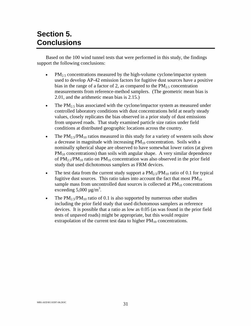
Based on the 100 wind tunnel tests that were performed in this study, the findings

support the following conclusions:

1. PM2.5 concentrations measured by the high-volume cyclone/impactor system used to develop AP-42 emission factors for fugitive dust sources have a positive bias by a factor of 2, as compared to the PM2.5 concentration measurements from reference-method samplers. (The geometric mean bias is 2.01 and the arithmetic mean bias is 2.15.)

2. The PM2.5 bias associated with the cyclone/impactor system as measured under controlled laboratory conditions with dust concentrations held at nearly steady values, closely replicates the bias observed in the prior EPA-funded field study at distributed geographic locations across the country.

3. The PM2.5/PM10 ratios measured in the current study for a variety of western soils show a decrease in magnitude with increasing PM10 concentration. Soils with a nominally spherical shape are observed to have somewhat lower ratios (at given PM10 concentrations) than soils with angular shape. A very similar dependence of PM2.5/PM10 ratio on PM10 concentration was also observed in the prior field study that used dichotomous samplers as FRM devices.

4. The test data from the current study support a PM2.5/PM10 ratio of 0.1 for typical fugitive dust sources. This ratio takes into account the fact that during AP-42 source tests most PM10 sample mass from uncontrolled dust sources is collected at plume core PM10 concentrations exceeding 5,000 µg/m3.

5. The PM2.5/PM10 ratio of 0.1 is also supported by numerous other studies including the prior field study that used dichotomous samplers as reference devices. It is possible that a ratio as low as 0.05 (as was found in the prior field tests of unpaved roads) might be appropriate, but this would require extrapolation of the current test data to higher PM10 concentrations.

The results of this project are needed to ensure development of the most accurate

PM2.5 and PM10 fugitive dust emissions inventories that are possible for regional haze regulatory purposes. In particular, a reduction in the quantity of dust apportioned to the fine versus coarse size modes will significantly affect models for visibility and long-range transport.

The results will also be helpful in developing accurate emission inventories for PM

nonattainment, maintenance, and action plan areas in the WRAP region. Finally, if appropriate, results may be used to seek modifications to the EPA’s AP-42 emission

MRI-AED\R110397-06.DOC iv

factors to ensure widespread availability of the most recent and accurate scientific information.

MRI-AED\R110397-06.DOC v

Contents Preface................................................................................................................................. ii Figures............................................................................................................................... vii Tables................................................................................................................................ vii Section 1. Introduction.......................................................................................................1 Section 2. Test Facility and Air Samplers .........................................................................4

2.1 Aerosol Test Facility.................................................................................4 2.2 Air Samplers .............................................................................................6 2.3 Test Matrix..............................................................................................10

Section 3. Pretest Activities .............................................................................................13

3.1 Test Protocol and Quality Assurance Project Plan .................................13 3.2 Test Dust Sample Collection and Handling............................................14

Section 4. Test Results.....................................................................................................20

4.1 Phase I......................................................................................................20 4.2 Phase II ...................................................................................................24

Section 5. Conclusions.....................................................................................................31 Section 6. References.......................................................................................................32 Appendices Appendix A—Summaries of Test Data Appendix B—QA/QC Activities

MRI-AED\R110397-06.DOC vi

Figures Figure 1. Cyclone/Impactor ................................................................................................2 Figure 2. MRI Flow Tunnel/Test Chamber ........................................................................5 Figure 3. Return Line to Wind Tunnel Blower...................................................................5 Figure 4. Fluidization System for Injecting Fine Fraction Dust

Into the Flow System........................................................................................6 Figure 5. Test Chamber Interior With Flow Straightener...................................................8 Figure 6. Partisol, Cyclone/Impactor, and DustTrak Inlets in Exposure Section ...............9 Figure 7. View of Partisol, Cyclone, and DustTrak Inlets

Through Observation Window .........................................................................9 Figure 8. Partisol Sampler Bodies Below Exposure Section of Wind Tunnel .................10 Figure 9. Sampling Procedure for Collecting Test Soil or Road Surface Material .........16 Figure 10. Agricultural Texture of Test Soils...................................................................19 Figure 11. Correlation Between Cyclone/Impactor and Partisol

PM2.5 Concentrations ......................................................................................23 Figure 12. PM2.5/PM10 Ratio vs. PM10 Concentration from Prior Field Study.................25 Figure 13. Ratio of DustTrak to Partisol PM10 Concentration Versus Average PM10

Concentration..................................................................................................26 Figure 14. PM2.5/PM10 Ratio Versus PM10 Concentration................................................28 Figure 15. Example Peak (6-sec) Plume PM10 Concentrations at Roadside Plume

Profiling Location...........................................................................................30

Tables Table 1. Air Samplers Used for Testing .............................................................................7 Table 2. Preliminary Test Matrix......................................................................................10 Table 3. Test Soils for Phase II.........................................................................................12 Table 4. Annotated Outline for Combined Test Protocol/QAPP......................................13 Table 5. Properties of Test Soils .......................................................................................18 Table 6. List of Tests Performed in Phase I......................................................................21 Table 7. List of Tests Performed in Phase II ....................................................................22

MRI-AED\R110397-06.DOC vii

Section 1. Introduction

The WRAP Dust Emissions Joint Forum (DEJF) is engaged in gathering and improving data pertaining to the PM2.5 and PM10 components of fugitive dust emissions. Most of the PM2.5 emission factors in EPA’s AP-42 guidance for fugitive dust sources [1] were determined by using high-volume samplers fitted with a cyclone precollector and cascade impactor. Under the same conditions, the PM2.5 mass measured using these cyclone/cascade impactors should be nearly identical to the mass collected using an ambient PM2.5 sampler that meets EPA ambient air monitoring requirements.

The MRI cyclone/impactor system (see Figure 1) has been recognized as the standard

method to characterize fugitive dust emissions for EPA and to develop predictive emission factor equations for AP-42. A sample of particles is drawn at a flow rate of 34 m3/hr (20 acfm) into a directional probe tip with an inlet velocity of 2.2 m/s (5 mph) and then through a cyclonic preseparator to remove particles larger than 15 µm in diameter. The PM10 in the exit airflow from the cyclone is channeled through multiple impactor stages before being collected on a back-up filter, from which time-integrated PM10 and PM2.5 concentrations can be calculated.

Historically, data from the MRI high-volume cyclone/impactor system have

provided the basis for PM2.5/PM10 ratios that have been published by EPA in AP-42 for various categories of fugitive dust sources. The advantage of the high volume cyclone/impactor systems relates to its directional sampling capability and higher analytical sensitivity for particle size measurement. However, particle bounce from the cascade impactor stages to the backup filter may have resulted in higher PM2.5 measurements than the actual PM2.5 concentrations, even though steps were taken by MRI to minimize particle bounce. Those steps included halving the flow rate, greasing the substrates prior to use, and limiting the sampling time so that substrates are not overloaded with collected particle mass.

Some comparative data collected in dust plumes downwind of paved and unpaved

roads in the late 1990s indicate that PM2.5/PM10 ratios determined with other particle sizing systems produced consistently lower ratios than with the cyclone/impactor system. This comparative particle sizing work was performed by MRI under contract to EPA [2]. As a result, modifications to reduce the ratios were made by EPA to the appropriate sections of AP-42.

Even with the adjusted particle size ratios imbedded in the current version of AP-42,

there is still evidence of a potential bias due to residual measurement error associated with particle bounce in the high-volume cascade impactor system. This possible measurement error may help to explain why the AP-42-based PM2.5 emission estimates seem to show about 20 percent of the fugitive dust mass is in the fine fraction, while ambient air monitoring data suggest that it may be on the order of 10 percent [3].

MRI-AED\R110397-06.DOC 1

Figure 1. Cyclone/Impactor In the first testing phase of this project, PM2.5 measurements using the high-volume

cascade impactors were compared to simultaneous measurements obtained using EPA reference-method samplers for PM2.5. These tests were conducted in a flow-through wind tunnel and exposure chamber, where concentration level and uniformity were controlled. The results of the tests provide the basis for quantifying more effectively any sampling bias associated with the cascade impactor system.

With the same test setup, a second phase of testing was performed with reference

method samplers, for the purpose of measuring PM2.5 to PM10 ratios for fugitive dust from different geologic sources in the West. This testing provided needed information on the magnitude and variability of this ratio, especially for source materials that are recognized as problematic with regard to application of mitigative dust control measures.

The results of this project are needed to ensure the most accurate PM2.5 and PM10

fugitive dust emissions inventories that are possible for regional haze regulatory purposes, given the available resources and the significant contribution of fugitive dust to visibility impairment. In particular, the results of this project may affect the quantity of dust apportioned to the fine versus coarse size modes, which have significantly different effects on visibility and long-range transport potentials. The results will also be helpful


in developing accurate emission inventories for PM nonattainment, maintenance, and action plan areas in the WRAP region. Finally, if appropriate, results may be used to seek modifications to the EPA’s AP-42 emission factors to ensure widespread availability of the most recent and accurate scientific information.


Section 2. Test Facility and Air Samplers 2.1 Aerosol Test Facility

The testing was conducted in the Aerosol Test Facility (ATF) in Building 2 at MRI’s Deramus Field Station in Grandview, Missouri. This system for generation and control of dust concentrations in an exposure chamber used equipment similar to that used in the recent performance evaluation of the MetOne GT-641 aerosol monitor [4] for use at Owens Lake, except that the MRI ATF is a recirculating flow system rather than a once-through system. The recirculation feature of the ATF promotes the establishment of well-mixed and steady target aerosol concentration levels in exposure section where the PM10 and PM2.5 monitors are positioned. The ATF also limits the consumption of test dust so that much smaller amounts of starting soil or road dust samples are sufficient for extensive testing.

The MRI test facility consists of a push-through flow system (3 ft by 3 ft cross

section) with an exposure chamber at the downstream end of the flow tunnel, as shown in Figure 2. The flow system can be operated at low air speeds (as low as 0.5 m/s), using an electronic motor speed controller. An 18-in diameter air return loop connects the outlet of the exposure chamber with the inlet to the blower, as shown in Figure 3. In this study, the tunnel was operated at a speed of 1 m/s (2 mph). The wind speed was highly uniform in the core of the flow (into which the inlets to the air samplers were placed). When a Kestral vane anemometer was used to measure the wind speed at the center points of nine equal areas of the tunnel cross-section, all measured point values were within about 10 percent of the average value.

A fluidized bed injects dust through a vertical copper tube (1-in internal diameter)

into the return line to the blower inlet that feeds the flow tunnel (Figure 4). The fluidized bed aerosolizes fine dust from samples of loose, dry soil from a cylindrical glass container (Puff cartridge) that is 10.2 cm tall and 5.5 cm internal diameter. A glass fiber filter is sandwiched between screens at the bottom of the chamber, and a conical section is positioned on top of the screens, directing the dust material to a circular area in the center of the screen. The fluidization rate is controlled by the upward airflow through the bed. The injection point to the tunnel flow is just downstream of the center of an 8-in orifice in the 18-in return line. The turbulent effluent from the orifice aids in mixing the injected dust into the tunnel airflow.

The PM10 dust concentration in the exposure chamber is continuously tracked with a

TSI Model 8520 DustTrak monitor that draws air from the centerline position in the exposure section. The DustTrak sampling line was standard equipment supplied by TSI. Based on a 9-point equal-area profile transecting the core of the flow, the PM10 concentration at each point is within 10 percent of the average value. A second DustTrak monitor (with its own sampling line) tracks the PM2.5 concentration at the centerline.


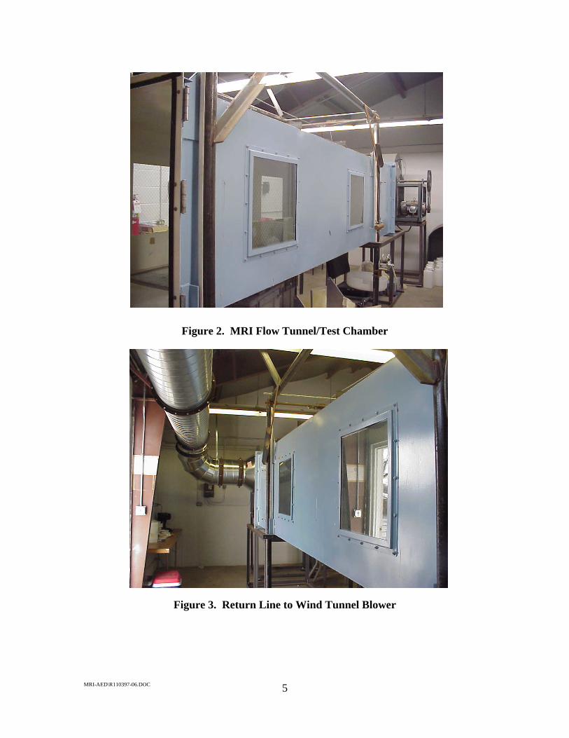
Figure 2. MRI Flow Tunnel/Test Chamber

Figure 3. Return Line to Wind Tunnel Blower


Figure 4. Fluidization System for Injecting Fine Fraction Dust Into the Flow System

2.2 Air Samplers Table 1 lists the air sampling equipment that was used in the two testing phases. The

EPA reference method samplers [5] consisted of Rupprecht & Patashnick Model 2000 Partisols for PM2.5 and PM10 measurements. The approximately 3 ft by 3 ft working cross section of the exposure chamber (Figure 5) and the two sampling stations within the chamber provided adequate space for the inlets of two cyclone/impactors, two Partisol samplers, and two DustTRAKs, depending on the requirements of the test being performed.

The MRI cyclone/impactor system, shown earlier in Figure 1, consists of a Sierra Model 230 cyclone with a directional intake and a Sierro Model 230CP three-stage slotted-type cascade impactor. When operated at 20 acfm, the cyclone has an aerodynamic cut point of 15 microns, and the cascade impactor stages have cut points of 10.2, 4.2, and 2.1 microns, respectively [2]. The slotted glass fiber substrates were coated with a thin film of grease before tare weighing (using the same procedure as in the past), to mitigate against particle bounce problems. For the same reason, care was taken not to overload the substrates with collected dust. Pretest estimation of the dust loading on the impactor stages must take into account that the PM10 sample is distributed over three separate impactor stages plus the back-up filter when the cyclone is operated at 20 acfm. Typically, the cyclone/impactor system has been utilized to generate PM2.5/PM10 ratios that can be used in combination with PM10 plume profiles to generate PM2.5 emission factors.


Table 1. Air Samplers Used for Testing

Phase No. in use Sampler Manufacturer/model Flow rate Comments

1 2 Cyclone preseparators

Sierra Model 230 CP 20 acfm Third stage has D50 cut of 2.1 µmA, which MRI has used surrogate for PM2.5.

2 Multistage impactor

Sierra Model 230 20 acfm First three stages used.

2 Partisol (FRM) R&P Model 2000 16.7 alpm Device uses WINS impactor to provide PM2.5 cut point.

2 DustTrak TSI Model 8520 5 alpm Used to continuously track concentration level and uniformity within exposure chamber

2 2 Partisol (FRM) R&P Model 2000 16.7 alpm Reference sampler uses WINS impactor to provide PM2.5 cut point.

2 Partisol (FRM) R&P Model 2000 16.7 alpm Reference sampler uses dichot inlet, which has D50 cut point of 10 µmA. Sampler is fitted with R&P part to bypass WINS impactor.

2 DustTRAK TSI Model 8520 5 alpm Used to continuously track concentration level and uniformity within exposure chamber.


Figure 5. Test Chamber Interior With Flow Straightener (Viewed from downstream end of exposure section)

EPA reference-method R&P Partisol analyzers were used to measure the

concentrations of PM10 and PM2.5 in the dust exposure chamber. The chamber was large enough to accommodate four Partisol inlets and two cyclone/impactor inlets (see Figures 6 and 7). By locating sampler inlets in opposing quadrants at the two sampling stations, any interference effects were negligible. The low flow in the exposure section of the wind tunnel minimized the propagation of turbulent wakes created by the sampling inlets. In Figure 6, the large opening at the rear of the tunnel is the inlet to the 18-in diameter return line. The bodies of the air samplers were placed underneath the exposure chamber (Figure 8).

It should be noted that because the sampling systems (except for the DustTrak

monitors) involved collection of PM on filters (and impactor substrates), the measured concentrations represented averages over each test period. With regard to the filter medium, a fibrous rather than a membrane-type filter was used for better retention of dust particles. Whatman EPM 2000 glass fiber filter and impactor substrate media were used throughout the testing.

Prior to testing, required filter and impactor substrate media were prepared for air

sampling. A temperature- and humidity-controlled gravimetrics laboratory was used for obtaining tare and final weights of filters and greased impactor substrates. The


temperature and humidity were maintained within the limits recommended by the EPA for filter weighing in association with ambient PM monitoring [6].

Cyclone 1

Cyclone 2

Partisol B

Partisol A

Partisol D

DustTRAK Sampling T b

Partisol C

Figure 6. Partisol, Cyclone/Impactor, and DustTrak Inlets in Exposure Section (as viewed from upstream)

Figure 7. View of Partisol, Cyclone, and DustTrak Inlets Through Observation Window


Figure 8. Partisol Sampler Bodies Below Exposure Section of Wind Tunnel

2.3 Test Matrix Table 2 shows the matrix of tests that were specified in the scope of work for this

project. At least 10 percent of tests utilized “field” blanks for all particle collection media, as is customary to meet quality control requirements.

Table 2. Preliminary Test Matrix

Phase Source materials Concentration

levels Replication

Total No. of tests Sampling media used

1 3

(Arizona road dust—coarse and fine,

Owens Lake surface material)

3

(Low, moderate, high)

3

(triplicates)

27 8x10 filters 4 x 5 substrates 47-mm filters plus > 10% field blanks for all media

2 5 3 3 45

(Representative soils or road surface

materials)

(low, moderate, high)

(triplicates)

47-mm filters plus > 10% field blanks


2.3.1 Phase I—AP-42 PM2.5 Emission Factor Evaluation

As indicated in Table 2, three dust source materials were tested under Phase I. Owens Dry Lake surface soil was used to provide one dust source material. The other two dust source materials were reference standards referred to as Arizona road dust, coarse and fine fractions. Arizona road dust is ground from Arizona sand using ball mills, elutriation, and blending to achieve reproducible size distributions for a variety of applications including performance testing of automotive air cleaners.

In order to entrain a steady stream of fine particles from the Arizona road dust

samples, it was necessary to add a small amount of sand to the dust generation chamber. Because of the fine texture of Arizona road dust (both size fractions consisting entirely of particles smaller than 75 microns), it is impractical to aerosolize these test dusts in any consistent fashion without adding sand to the fluidized bed. The powder tends to clump because of strong interparticle binding forces. If this powder were exposed to the atmosphere, its release as fine particles would require vigorous mechanical contact (e.g., rolling tires) or sandblasting by saltating particles in the size range of 100 microns.

Fixed PM10 concentration levels in the range of 1,000, 2,500, and 5,000 micrograms per cubic meter (each with its naturally occurring PM2.5 level) were tested. These PM10 concentration levels were selected as representative of dust plume concentrations under which major particle mass contributions to plume samples occur in emission factor development.

The PM10 concentration level during each 20- to 120-min test was maintained as

closely as possible to a predetermined target value. This was accomplished by adjusting the airflow in the dust aerosolization system. Tests at each concentration level were performed in triplicate.

Because filter-based reference-method PM2.5 monitors with relatively low sampling

rates were used in the study, care was taken so that the test periods were sufficient so that minimum quantifiable mass is collected on the PM2.5 (47-mm) filters. However, certain test soils did not have sufficient dust emission potential to achieve the higher concentrations using the dust aerosolization system. 2.3.2 Phase II—PM2.5 to PM10 Ratios for Different Soil Samples

In Phase II, reference-method Partisols measured both PM10 and PM2.5

concentrations. Once again, fixed PM10 concentrations (each with its naturally occurring PM2.5 level) were tested.

In accordance with the test protocol and Quality Assurance Project Plan (QAPP),

MRI measured the ratio of PM2.5 to PM10 for fugitive dust from different geologic soil types. A total of seven source materials were tested, which was two more than originally specified in the scope of work. Test results included the calculation of the average PM2.5


concentration and the collocated PM10 concentration. It was intended that any variation in PM2.5/PM10 ratio be evaluated as a function of the test soil properties (for example, position in soil texture triangle).

As stated under Section 3, MRI worked with the DEJF in selecting the individual soil types to be tested. These soils were provided by WRAP members. The types and locations of test soils for Phase II are listed in Table 3.

Table 3. Test Soils for Phase II Code State Location Type of material AK Alaska MAT-SU Knik River Bed

Sediments

AZal Arizona Phoenix Area

Alluvial Channel

AZag Arizona Phoenix Area

Agricultural Soil

NMr New Mexico Las Cruces Landfill

Road Dust

NMs New Mexico Radium Springs

Grazing Soil

SS California Salton Sea

Shoreline Soils

WY Wyoming Thunder Basin Mine Barrow Pit for Access Road Surface Material


Section 3. Pretest Activities

3.1 Test Protocol and Quality Assurance Project Plan

Prior to the testing, MRI submitted to the DEJF a combined test protocol/QAPP [7] according to EPA standards. The test protocol included design of the dust generation system and exposure chamber, specification of monitoring equipment, procedures for sampling, testing, and data analysis, and other procedures or design information essential to the completion of the project. Because the results of this project may be considered in revisions to EPA-published emission factors, adherence to EPA quality assurance documentation procedures was an important part of this project. The test protocol and quality assurance plans complied with EPA standards and will specify all procedures to be followed in collecting, recovering, transferring, and analyzing samples.

These plans were prepared in compliance with EPA document QA/R-5 (EPA Requirements for QA Project Plans) as well as the guidance document QA/G-5 (Guidance for Quality Assurance Project Plans). To aid the EPA in review of the plans, the documents were structured to mimic the required groups and elements of QA/G-5.

The outline for the combined plan is given as Table 4. Note that the labels in parentheses (such as “A3”) after each section refer to the group/element labels in QA/G-5 and are included to facilitate review.

Table 4. Annotated Outline for Combined Test Protocol/QAPP Preface Distribution of QAPP (A3)—includes list of persons who have received the QAPP, signature approval page, and revision history of the document Figures—includes Test Facility Schematic, Sampler Locations, Amendment Record for QAPP, Corrective Action Report Form Tables—includes Data Quality Objectives, Test Design, Test Schedule, Critical and Non-Critical Measurements, and Quality Control Procedures for Sampling Media, Quality Control Procedures for Sampling Equipment, Quality Assurance for Miscellaneous Equipment Section 1. Project Management (A)

1.1 Project Organization (A4) 1.2 Introduction/Background (A5) 1.3 Project Task Description (A6) 1.4 Quality and Measurement Objectives (A7) 1.5 Project Narrative 1.6 Special Training Requirements/Certification (A8) 1.7 Documentation and Records (A9)


Section 2. Measurement/Data Acquisition (B)

2.1 Sampling Process Design (Experimental Design) (B1) 2.2 Sampling Methods Requirements (B2) 2.3 Sample Handling and Custody Requirements (B3) 2.4 Analytical Methods Requirements (B4) 2.5 Quality Control Requirements (B5) 2.6 Instrument/Equipment Testing, Inspection, and Maintenance Requirements

(B6) 2.7 Instrument Calibration and Frequency (B7) 2.8 Inspection/Acceptance Requirements for Supplies and

Consumables (B8) 2.9 Data Acquisition Requirements (B9) 2.10 Data Management (B10)

Section 3. Assessment/Oversight (C)

3.1 Assessments and Response Actions (C1) 3.2 Corrective Action 3.3 Reports to Management (C2) 3.4 Task 6—Project Report

Section 4. Data Validation and Usability (D)

4.1 Data Review, Validation, and Verification Requirements (D1) 4.2 Validation and Verification Methods (D2) 4.3 Reconciliation With User Requirements (D3)

Section 5. References

3.2 Test Dust Sample Collection and Handling

Soil and road surface material samples for the subject testing were collected from a variety of locations. Some existing samples were available from prior studies, such as those involving reference Arizona road dust and surface materials from Owens Lake. However, the remaining samples came from other sources. MRI worked with the DEJF to determine the most appropriate types of samples to be used in this study. Samples that were not available from other studies were collected specifically for this study. Again, MRI worked with the DEJF to determine the best locations and surfaces from which to collect such samples.

It was recommended that test materials represent troublesome western soils that were

observed to be high dust emitters. It was pointed out that soils with high dustiness potential tend to be subject to frequent mechanical disturbances by agricultural operations, construction operations, or other operations involving vehicle travel across exposed areas. Therefore, only samples of unconsolidated (uncrusted and uncompacted) soils or road aggregate materials are likely to have high dustiness potential.


Two 5-gal containers of each dusty soil or aggregate material were requested to sustain a series of tests to determine PM2.5/PM10 ratios under a variety of test conditions. It was stated that only loose, dry (less than 1% moisture) soils should be collected. For soils, the depth of sampling should not exceed 2 in (5 cm). All particles greater than 4-mesh (0.47 cm) are considered nonerodible, and so it was instructed that they be removed from the sample by dry sieving prior to shipment of the sample to MRI.

Members of the WRAP (e.g., state, local, and tribal air quality professionals)

collected and shipped the samples to MRI. A soil screening device, soil collection procedures, and associated data forms were provided by MRI as specified in the test protocol and QAPP. An example procedure is supplied in Figure 9.

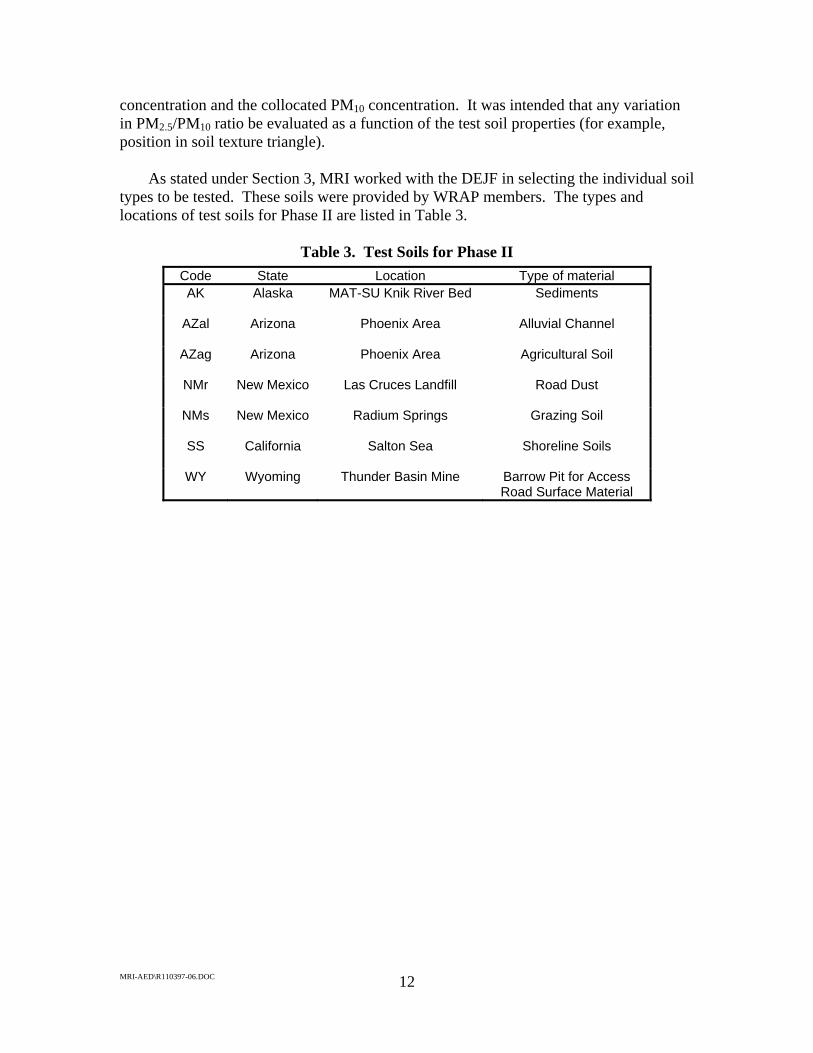
The properties of the test soils provided for this study are summarized in Table 5.

This includes the moisture content and the dry silt content (fraction passing a 200-mesh screen upon dry sieving) using the procedure specified in AP-42 [1]. The dry silt content has been used as a surrogate for dustiness in the AP-42 emission factor equations for fugitive dust.

A standard agricultural soil analysis [8] was performed on well-mixed subsamples of each test material. When plotted on the soil texture triangle, most of the samples fell into a relatively small region, as shown in Figure 10. This texture region is characterized by high wet silt content and moderate sand content.


Two 5-gal containers of a dusty soil or aggregate material are needed for each test material

to sustain a series of tests to determine PM2.5/PM10 ratios under a variety of test conditions. Only loose, dry (less than 1% moisture) soils should be collected. For soils, the depth of sampling should not exceed 2 in (5 cm). All particles greater than 4-mesh (0.47 cm) are considered nonerodible and should be removed from the sample by dry sieving prior to shipment of the sample to MRI. MRI will provide a special screen for this purpose.

Collection of Surface Soil Samples

The following steps outline the procedure to collect a two 5-gal soil samples of pulverized

soil from an open area:

1. Define and document the area of interest: a. Size of sampled field b. Lat/long or UTM coordinates of approximate field centroid c. Land use and recent disturbance history d. Recent and current weather e. Observed field surface texture/appearance f. USDA surface soil classification

2. Collect surface soil sample

a. Collect two 5-gal containers of soil by compositing approximately equal amounts from a minimum of 10 locations in the same agricultural field

i. Use a straight-edge shovel to collect each incremental sample ii. Sample to a loose soil depth not exceeding 2 in (5 cm) iii. Empty each incremental sample from the shovel into the screen that covers a

5-gal plastic bucket iv. Measure the approximate volume of coarse material that is screened from the

total composite sample b. Seal the bucket lid using tape and label the bucket with a permanent marker

i. Field name ii. Date/time of collection iii. Sample number corresponding to the data sheet iv. Name of person collecting the sample

c. Document the sample collection on a data sheet i. Location of sampled areas (e.g., GPS coordinates, sketch of field locations) ii. Approximate area (sq ft) from which each incremental sample is taken Figure 9. Sampling Procedure for Collecting Test Soil or

Road Surface Material


Collection of Surface Samples of Unpaved Road Aggregate

The following steps outline the procedure to collect two 5-gal samples of surface aggregate from an unpaved road.

3. Define and document the area of interest:

a. Length and width of sampled road segment b. Lat/long or UTM coordinates of approximate road segment centroid c. Road use and recent maintenance history d. Recent and current weather e. Observed road surface texture/appearance f. Road aggregate type and origin

4. Collect surface soil sample

a. Collect 5 gal of loose surface material by compositing equal amounts of uncrusted soil from a minimum of 10 edge-to-edge steps across in the traveled area of the road

i. Use a whisk broom and dust pan ii. Sample to a 1 cm depth or to the hardpan iii. Empty each incremental sample from the dust pan into the screen that covers

a 5-gal plastic bucket b. Seal the bucket lid using tape and label the bucket with a permanent marker

i. Road name ii. Date/time of collection iii. Sample number corresponding to the data sheet iv. Name of person collecting the sample

c. Document the sample collection on a data sheet i. Location of sampled areas (e.g., GPS coordinates, sketch of field locations) ii. Approximate area (sq ft) from which each incremental sample is taken

Figure 9. Sampling Procedure for Collecting Test Soil or Road Surface Material (Concluded)


Table 5. Properties of Test Soils

Code State Location Type of material Moisture

content (%) Dry silt

content (%) Dry Silt

rank

TF Arizona – Standard Test Dust—Fine

– – –

TC Arizona – Standard Test Dust—Coarse

0.60 87.6 1

AK Alaska MAT-SU Knik River

Bed

Sediments 0.80 8.69 6

AZal Arizona Phoenix Area

Alluvial Channel 0.33 17.3 3

AZag Arizona Phoenix Area

Agricultural Soil 1.06 21.6 2

NMr New Mexico

Las Cruces Landfill

Road Dust 1.27 12.2 4

NMs New Mexico

Radium Springs

Grazing Soil 0.47 10.9 5

OW California Owens Dry Lake

Lakebed Soil 0.27 3.14 9

SS California Salton Sea Shoreline Soils 5.46* 3.63 8

WY Wyoming Thunder Basin Mine

Barrow Pit for Access Road

Surface Material

2.47* 6.83 7

* Required drying prior to testing.


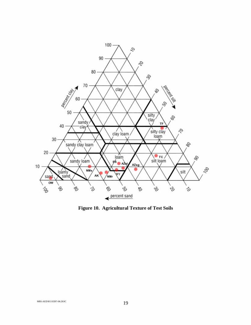
Figure 10. Agricultural Texture of Test Soils


Section 4. Test Results

The list of tests that were performed is shown in Tables 6 and 7 for Phase I and Phase II tests, respectively. The Phase I tests were performed in March and April of 2005. The Phase II tests were performed in June through August of 2005. Although the scope of work specified five test materials for Phase II, seven materials were tested (with the last two at one target concentration level). Although it was desired to test the last two materials in the PM10 concentration range of 5,000 µg/m3, the perimeter soil from the Salton Sea was found to have a low dustiness index, so that only a concentration in the range of 1,000 µg/m3 could be achieved.

A total of 100 individual tests were performed, including 17 blank runs (for quality assurance purposes). The raw and intermediate test data are summarized in the tables presented in Appendix B of this report. Static blank filters were collected by loading filters into samplers with inlets positioned in a still air environment. Dynamic blank filters were collected by loading filters into samplers with inlets positioned in a moving air environment. In neither case was air drawn through the samplers. 4.1 Phase I

As noted above, the testing in Phase I was directed to determining whether a bias existed in the PM2.5 concentrations historically measured by the high-volume cyclone/impactor system in fugitive dust plumes. Data from the cyclone/impactor system were balanced against dichotomous sampler results [2] in developing particle size multipliers for EPA’s fugitive dust emission factor equations currently published in AP-42.

In Phase I, the flow through the dust generation chamber was varied as needed to maintain the target PM10 concentration in the exposure section of the wind tunnel, as measured by the DustTrak monitor with an inlet line extended to the centerline position. An auger was used periodically to add test soil to the chamber, once the supply was depleted to less than half of the original amount added at the beginning of a test.

Prior to each test series, the wind tunnel was purged with clean air that was exhausted outside the building, to remove any loose accumulation of dust on the interior surfaces of the flow system. In addition, all sampler flow rates were checked, as well as the impactors in the PM2.5 Partisol samplers and the PM2.5 DustTrak monitors.

The results of the Phase I testing are summarized in Figure 11, which shows that the PM2.5 concentrations measured by the cyclone/impactor system are consistently biased by a factor of about 2 relative the PM2.5 concentrations measured by the Partisol samplers. (The geometric mean bias is 2.01, and the arithmetic mean bias is 2.15.) This bias is also reflected in the PM2.5/PM10 ratios measured by the cyclone/impactor system in relation to the reference samplers. The one exception occurs for the Arizona course test dust at the high concentration, for which the ratio is nearly a factor of 4.


Table 6. List of Tests Performed in Phase I

Date Run Test dust

Duration of test (min)

Actual PM10 concentration (µg/m3)a

3/2/2005 1 AZ Fine Dust 60 2220 3/24/2005 2 AZ Fine Dust 60 1060 3/29/2005 3 AZ Fine Dust 60 1080 3/29/2005 4,5 AZ Fine Dust 120 1190, 1120 3/29/2005 6 Dynamic Blank Run – – 3/30/2005 7 AZ Fine Dust 120 1020 3/30/2005 8,9,10 AZ Fine Dust 15 5001, 5600,4990 3/30/2005 11 Static Blank Run – – 4/1/2005 12,13,14 AZ Coarse Dust 15 4580, 3860, 4850 4/1/2005 15 Static Blank Run – – 4/6/2005 16,17,18 AZ Coarse Dust 60 2210, 2170, 1950 4/6/2005 19 Dynamic Blank Run – – 4/7/2005 20,21,22 AZ Coarse Dust 120 575, 582, 348 4/7/2005 23 Static Blank Run – – 4/21/2005 24 Owens Dry Lake Bed 20 3460 4/21/2005 25 Owens Dry Lake Bed 22 2840 4/21/2005 26 Owens Dry Lake Bed 20 3720 4/21/2005 27,28,29 Owens Dry Lake Bed 60 2350 4/21/2005 30 Static Blank Run – – 4/22/2005 31,32,33 Owens Dry Lake Bed 120 492, 559, 464 4/22/2005 34 Dynamic Blank Run – – a PM10 concentrations measured by DustTRAK monitor through run WR-15 and by

Partisol samplers for subsequent tests.



Table 7. List of Tests Performed in Phase II

Date Run Test dust Duration of test (min)

Actual PM10 concentration

(µg/m3) 6/9/2005 35 AZ Ag Field 60 927 6/10/2005 36,37 AZ Ag Field 60 874, 889 6/10/2005 38,39,40 AZ Ag Field 40 2676, 3246, 2473 6/10/2005 41,42,43 AZ Ag Field 20 5197, 4576, 4852 6/10/2005 44 Dynamic Blank Run – – 6/14/2005 45 Knik River Sediment 40 783 6/14/2005 46 Knik River Sediment 60 340 6/14/2005 47 Knik River Sediment 120 487 6/14/2005 48,49 Knik River Sediment 20 3658, 4800 6/14/2005 50 Dynamic Blank Run – – 6/16/2005 51,52 Knik River Sediment 40 3119, 3254 6/16/2005 53,54 Knik River Sediment 80 1211, 1316 6/16/2005 55 Dynamic Blank Run – – 6/17/2005 56,57,58 Las Cruces Landfill Road 20 5807, 5736, 5737 6/17/2005 59,60 Las Cruces Landfill Road 40 2784, 2719 6/17/2005 61 Dynamic Blank Run – – 6/22/2005 62 Las Cruces Landfill Road 40 2662 6/22/2005 63,64,65 Las Cruces Landfill Road 80 1050, 1000, 1011 6/22/2005 66 Dynamic Blank Run – – 6/23/2005 67 Thunder Basin Barrow Pit 40 2600 6/23/2005 68,69 Thunder Basin Barrow Pit 40 2473, 2180 6/23/2005 70,71 Thunder Basin Barrow Pit 60 1270, 682 6/23/2005 72 Dynamic Blank Run – – 6/24/2005 73 Thunder Basin Barrow Pit 60 1113 6/24/2005 74,75,76 Thunder Basin Barrow Pit 120 473, 616, 509 6/24/2005 77 Dynamic Blank Run – – 6/30/2005 78,79,80 AZ Alluvial Channel 20 6141, 6755, 6711 6/30/2005 81,82,83 AZ Alluvial Channel 40 3343, 3201, 2907 6/30/2005 84 AZ Alluvial Channel 80 1278 6/30/2005 85 Dynamic Blank Run – – 7/1/2005 86,87 AZ Alluvial Channel 80 1088, 1112 7/1/2005 88 Dynamic Blank Run – – 8/1/2005 89 Radium Springs 40 2605 8/1/2005 90,91 Radium Springs 40 2346, 2914 8/1/2005 92 Dynamic Blank Run – – 8/1/2005 93,94,95 Salton Sea 80 805, 595, 548 8/2/2005 96 Dynamic Blank Run – – 8/2/2005 97,98,99 AZ Ag Field 20 5475, 7087, 5603 8/2/2005 100 Dynamic Blank Run – –

I-AED\R110397-06.DOC 23

Figure 11. Correlation Between Cyclone/Impactor and Partisol PM2.5 Concentrations

y

0

0.5

1

5

2

5

3

5

4

5

0 1 2 3 4 5 6

PM 10 Concentration (mg/m3)

Cyc

lone

Con

cent

ratio

n / P

artis

ol C

once

ntra

tion

( PM

2.5

)

AZ FineAZ CoarseOwens DLB

MR

4.

3.

2.

1.


This bias was also observed in an EPA-funded field testing program [2] performed on dust emissions from paved and unpaved roads at three geographic locations across the country (Raleigh, North Carolina; Grandview, Missouri; Reno, Nevada). In that study, reference-method dichotomous samplers were used as the standard, with either Teflon (DT) or quartz fiber (DQ) filters. The bias in the PM2.5 measurements with the cyclone/impactor system was reflected in the calculated PM2.5/PM10 ratios as compared with the ratios calculated from the collocated dichotomous samplers.

As shown in Figure 12 for EPA-funded tests of unpaved roads, the PM2.5/PM10 ratios measured by the cyclone/impactors clustered around a value of 0.25, whereas the dichotomous samplers gave much lower values that decreased with increasing PM10 concentrations. Based on the test results from the EPA program, a new default value of 0.15 for the PM2.5/PM10 ratio was used to replace the previous value of 0.26 for dust emissions from unpaved roads. A default value of 0.15 was also recommended [2] for most of the other fugitive dust source categories, the exceptions being paved roads (0.25) and agricultural crops (0.20).

It is important to note that the PM10 concentrations in Figure 12 are averages during the testing rather than peak values encountered with each plume passage. Because vehicles passed the test site at the rate of about one per minute (with a plume passage time of less than 6 seconds), the peak values of PM10 concentration were at least 10 times the average values.

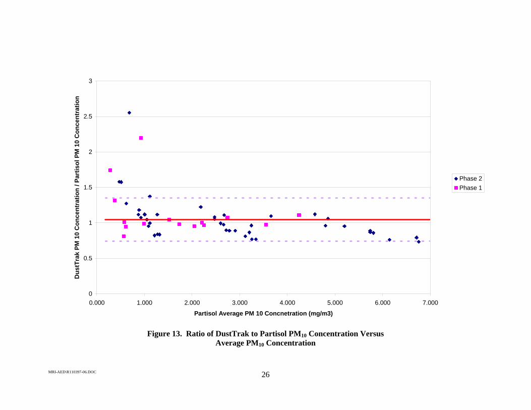
In the first test series of Phase I (through Test WR-15), a DustTrak monitor was used to continuously measure the PM10 concentration in the exposure section of the wind tunnel. Later, when a Partisol sampler was operated concurrently to measure the PM10 concentration, a running comparison was made between the DustTrak PM10 concentration and the Partisol PM10 concentrations, as shown in Figure 13. Except for PM10 concentrations below 1,000 µg/m3, all ratios fell within one relative standard deviation of 30 percent about the mean of 1.06. 4.2 Phase II

The purpose of the Phase II testing was to determine whether PM2.5/PM10 ratios measured with reference method samplers depend on (a) the test material [soil or road surface aggregate] that generates the dust, or (b) the dust concentration to which the samplers are exposed.

0

0.05

0.1

0.15

0.2

0.25

0.3

0.35

0.4

0.45

0.5

0 1000 2000 3000 4000 5000 6000 7000 8000 9000 10000

PM 10 Concentration (ug/m3)

PM 2

.5/ P

M 1

0 R

atio

CycloneDTDQ

Figure 12. PM2.5/PM10 Ratio vs. PM10 Concentration from Prior Field Study [2]


0

0.5

1

1.5

2

2.5

3

0.000 1.000 2.000 3.000 4.000 5.000 6.000 7.000

Partisol Average PM 10 Concnetration (mg/m3)

Dus

tTra

k PM

10

Con

cent

ratio

n / P

artis

ol P

M 1

0 C

once

ntra

tion

Phase 2Phase 1

Figure 13. Ratio of DustTrak to Partisol PM10 Concentration Versus Average PM10 Concentration

I-AED\R110397-06.DOC 26

MR


In this phase, known amounts of test material were added to the dust chamber at the beginning of the test, so the auger (used in Phase I to introduce additional material) was eliminated. Whenever the airflow through the dust suspension chamber was activated, it was held at a constant value of 19 lpm, so that the energy input to the dust generation process did not vary. Each test soil was manually dry sieved through a 20-mesh screen, to eliminate observed erratic behavior in the dust generation process. For example, when the Knik River Sediment was tested without presieving, highly variable results were obtained (Runs WR-45 through WR-47).

Prior to each test series, the wind tunnel was purged with clean air to remove any

loose accumulation of dust on the interior surfaces of the flow system. In addition, all sampler flow rates were checked, as well as the impactors in the PM2.5 Partisol samplers and the PM2.5 DustTrak monitors. The DustTrak impactors were regreased before proceeding.

The results of the Phase II testing are summarized in Figure 14. Although some data separation of different test materials is evident, there is an obvious tendency of the measured PM2.5/PM10 ratio to decrease with increasing PM10 concentration. One observation of note is that the results for the more spherical test soils (river sediment and alluvial channel) are separated from the results for the other materials, which are more angular in nature.

One possible explanation for the decrease in PM2.5/PM10 ratio with increasing PM10

concentration is the increased agglomeration of the coarse and fine modes of PM10.. This enhanced agglomeration would occur near the point of dust release from an open source. As the plume disperses, the PM10 concentration decreases because of enhanced deposition of the coarse mode and the PM2.5/PM10 ratio increases.

In specifying the appropriate PM2.5/PM10 ratio to associate with emission factor determination for fugitive dust sources, an important factor is the PM10 concentration range under which most of the plume mass is collected on sampler substrates. For uncontrolled emissions from unpaved roads, which accounts for the majority of PM10 emissions from mechanically generated dust across the country, most of the plume mass is obtained at concentrations exceeding 5,000 µg/m3.

0.000

0.050

0.100

0.150

0.200

0.250

0.300

0.350

0.400

0.450

0.000 1.000 2.000 3.000 4.000 5.000 6.000 7.000 8.000

PM 10 Concentration (mg/m3)

PM 2

.5 /

PM 1

0 R

atio

AZ Ag Soil

Knik RiverSediments

Las Cruces LandfillRoad

Thunder Basin Mine

AZ Alluvial Channel

Radium Springs

Salton Sea

Figure 14. PM2.5/PM10 Ratio Versus PM10 Concentration

I-AED\R110397-06.DOC 28

MR


An example of peak PM10 concentration data from uncontrolled road dust plumes is shown in Figure 15, which was obtained alongside an unpaved road at Ft. Riley, Kansas, in July 2005 [9]. Note that the alternate 6-sec peaks in this 20-pass test corresponded to 15-mph passes as opposed to the 30-mph passes. The latter passes correspond to the default vehicle speed used in AP-42 for the unpaved road emission factor equation. It should be noted that the peak 1-sec concentrations exceed the peak 6-sec concentrations by at least a factor of 3.

It is evident from Figure 14, that at PM10 concentrations above 5,000 µg/m3, at which most of the plume mass is collected for emission factor determination, the representative ratio of PM2.5/PM10 is 0.1. This conclusion is supported by the results of the earlier field testing program [2], which are shown above in Figure 12. The fact that the ratios from the reference-method samplers in the field study were as low as 0.05 is explained in part by the fact that the effective PM10 concentrations under which the samples were collected were in the range of 10,000 µg/m3 and above. In fact, Reference 2 states that dust plume core concentrations adjacent to unpaved roads often exceed 20,000 µg/m3. A PM2.5/PM10 of 0.1 is also consistent with observed data using FRM samplers during high-wind dust events on Owens Dry Lake [10].

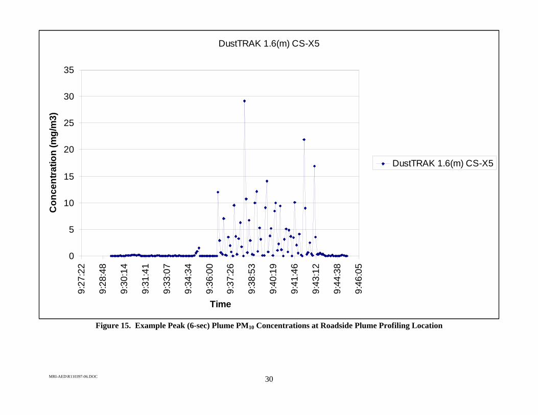
Figure 15. Example Peak (6-sec) Plume PM10 Concentrations at Roadside Plume Profiling Location


DustTRAK 1.6(m) CS-X5

0

5

10

15

20

25

30

359:

27:2

2

9:28

:48

9:30

:14

9:31

:41

9:33

:07

9:34

:34

9:36

:00

9:37

:26

9:38

:53

9:40

:19

9:41

:46

9:43

:12

9:44

:38

9:46

:05

Time

Con

cent

ratio

n (m

g/m

3)

DustTRAK 1.6(m) CS-X5

Section 5. Conclusions

Based on the 100 wind tunnel tests that were performed in this study, the findings support the following conclusions:

• PM2.5 concentrations measured by the high-volume cyclone/impactor system used to develop AP-42 emission factors for fugitive dust sources have a positive bias in the range of a factor of 2, as compared to the PM2.5 concentration measurements from reference-method samplers. (The geometric mean bias is 2.01, and the arithmetic mean bias is 2.15.)

• The PM2.5 bias associated with the cyclone/impactor system as measured under controlled laboratory conditions with dust concentrations held at nearly steady values, closely replicates the bias observed in a prior study of dust emissions from unpaved roads. That study examined particle size ratios under field conditions at distributed geographic locations across the country.

• The PM2.5/PM10 ratios measured in this study for a variety of western soils show a decrease in magnitude with increasing PM10 concentration. Soils with a nominally spherical shape are observed to have somewhat lower ratios (at given PM10 concentrations) than soils with angular shape. A very similar dependence of PM2.5/PM10 ratio on PM10 concentration was also observed in the prior field study that used dichotomous samplers as FRM devices.

• The test data from the current study support a PM2.5/PM10 ratio of 0.1 for typical fugitive dust sources. This ratio takes into account the fact that most PM10 sample mass from uncontrolled dust sources is collected at PM10 concentrations exceeding 5,000 µg/m3.

• The PM2.5/PM10 ratio of 0.1 is also supported by numerous other studies including the prior field study that used dichotomous samplers as reference devices. It is possible that a ratio as low as 0.05 (as was found in the prior field tests of unpaved roads) might be appropriate, but this would require extrapolation of the current test data to higher PM10 concentrations.


Section 6. References

1. USEPA. 1995. Compilation of Air Pollutant Emission Factors, AP-42. 6th Edition. Research Triangle Park, NC. [EPA’s emission factor handbook]

2. Midwest Research Institute. 1997. Fugitive Particulate Matter Emissions. Final report prepared for the U.S. Environmental Protection Agency, Office of Air Quality Planning and Standards. Research Triangle Park NC. April, 1997. [Prior emission factor field study for paved and unpaved roads, comparing performance of cyclone/impactor system with reference method samplers for PM2.5]

3. Pace, T. G. 2005. “Examination of Multiplier Used to Estimate PM2.5 Fugitive Dust Emissions from PM10.” Presented at the EPA Emission Inventory Conference. Las Vegas NV. April 2005. [Summarizes other field studies that can be used to develop PM2.5/PM10 ratios for fugitive dust emissions]

4. CH2M Hill. 2002. A Precision and Accuracy Assessment of the MetOne GT-641 Aerosol Monitoring Instrument. Prepared for the Los Angeles Department of Water and Power. Los Angeles, CA. February 2002. [Prior sampler comparison study utilizing wind tunnel and exposure chamber]

5. USEPA. 2004. List of Designated Reference and Equivalent Methods. National Exposure Research Laboratory, Research Triangle Park, NC. [Gives documentation approving FRM status of Partisol 2000 samplers]

6. USEPA. 1993. “National Primary and Secondary Ambient Air Quality Standards.” CFR Part 50. Washington, DC. [Specifies filter conditioning requirements]

7. Midwest Research Institute. 2005. Site-Specific Test and Quality Assurance Plan. MRI Project 110397. Kansas City, MO. March 10, 2005. [Test/QA Plan for this study]

8. Davies, C. 2005. “Sediment Particle Size Analysis.” University of Missouri, Kansas City, MO. [Describes soil analysis methods and results]

9. Midwest Research Institute. 2005. Technical Memorandum on the Field Study of Roadway Dust Capture on Tall Prairie Grass. Prepared for the Army Construction Engineering Laboratory. Champaign, IL. August 2005. [Example field study showing peak PM10 concentrations at plume profiling position downwind of unpaved road]


10. Ono, Duane. 2005. “Ambient PM2.5/PM10 ratios for Dust Events from the

Keeler Dunes.” Great Baron UAPCD, Bishop, CA. [Describes FRM test results for high-wind events on Owens Dry Lake.]


Appendix A Summaries of Test Data

MRI-AED\R110397-06.DOC

Table A-1. Test Data From Phase I

Concentration (mg/m3)

DustTRAKS Partisols Average Partisol

Cyclone/ Impactors

Average Cyclone

/Impactor PM-2.5/PM-10 Ratios

Run Test dust PM-10 PM-2.5 PM-10 PM-2.5 PM-2.5 PM-2.5 PM-2.5 DustTRAKS Partisols Cyclone/ impactors

Average cyclone/ impactor

WR-1 AZ Fine 2.15 0.6 0.595 1.15 1.125 0.28 0.5 0.51

0.589 1.1 0.52 WR-2 AZ Fine 2.29 1.06 0.701 0.645 1.1 1.075 0.46 0.28 0.48 0.48

0.588 1.05 0.48 WR-3 AZ Fine 2.1 1.05 [2.295] 0.627 1.12 1.110 0.50 0.30 0.58 0.58

0.627 1.1 0.57 WR-4 AZ Fine 1.19 0.581 0.333 0.318 0.525 0.530 0.49 0.27 0.5 0.51

0.302 0.535 0.51 WR-5 AZ Fine 1.12 0.385 0.332 0.296 0.56 0.524 0.34 0.26 0.46 0.45

0.26 0.488 0.44 WR-6 BLANK

WR-7 AZ Fine 1.02 0.323 0.248 0.241 0.506 0.475 0.32 0.24 0.42 0.42

0.234 0.444 0.42 WR-8 AZ Fine 4.95 1.46 1.613 1.426 2.455 2.385 0.29 0.29 0.46 0.47

1.238 2.314 0.47 WR-9 AZ Fine 5.6 1.77 1.693 1.613 3.144 2.982 0.32 0.29 0.49 0.48

1.533 2.82 0.47 WR-10 AZ Fine 4.99 1.44 1.338 1.290 2.408 2.391 0.29 0.26 0.45 0.46

1.242 2.373 0.46 WR-11 BLANK

WR-12 AZ Coarse 4.74 0.662 0.515 0.457 1.919 1.872 0.14 0.10 0.33 0.33

0.479 1.825 0.33 0.376

WR-13 AZ Coarse 4.5 0.615 0.591 0.566 2.108 1.905 0.14 0.13 0.37 0.36 0.503 1.701 0.34 0.603

WR-14 AZ Coarse 4.9 0.769 0.563 0.417 2.072 2.037 0.16 0.09 0.34 0.35 0.495 2.002 0.35 0.192

WR-15 BLANK

WR-16 AZ Coarse 2.21 0.395 2.209 0.385 0.378 0.764 0.710 0.18 0.17 0.31 0.30 0.371 0.656 0.29

WR-17 AZ Coarse 2.17 0.225 2.252 0.31 0.286 0.64 0.589 0.10 0.13 0.25 0.24 0.261 0.537 0.23

WR-18 AZ Coarse 1.95 0.182 2.045 0.264 0.213 0.556 0.520 0.09 0.10 0.24 0.24 0.162 0.483 0.23

WR-19 BLANK

WR-20 AZ Coarse 0.575 0.169 0.608 0.111 0.120 0.195 0.191 0.29 0.20 0.32 0.31 0.129 0.187 0.29

WR-21 AZ Coarse 0.582 0.16 0.577 0.14 0.122 0.217 0.210 0.27 0.21 0.31 0.32 0.104 0.202 0.33

WR-22 AZ Coarse 0.977 0.234 0.987 0.156 0.156 0.316 0.303 0.24 0.16 0.29 0.29 [0.053] 0.29 0.28

WR-23 BLANK

WR-24 Owens DLB 3.46 0.945 3.55 0.709 0.700 1.455 1.425 0.27 0.20 0.35 0.35 0.691 1.394 0.35

WR-25 Owens DLB 2.95 0.941 2.743 0.764 0.740 1.52 1.454 0.32 0.27 0.44 0.45 0.715 1.387 0.46

WR-26 Owens DLB 4.72 1.54 4.245 1.23 1.212 2.25 2.242 0.33 0.29 0.45 0.46 1.194 2.233 0.47

WR-27 Owens DLB 2.05 0.845 [0.932] 0.497 0.468 0.964 0.926 0.41 0.23 0.43 0.43 0.438 0.887 0.43

WR-28 Owens DLB 1.59 0.565 1.519 0.376 0.365 0.691 0.663 0.36 0.24 0.38 0.39 0.353 0.635 0.4

WR-29 Owens DLB 1.69 0.687 1.727 0.442 0.408 0.812 0.775 0.41 0.24 0.44 0.45

MRI-AED\R110397-06.DOC A-1

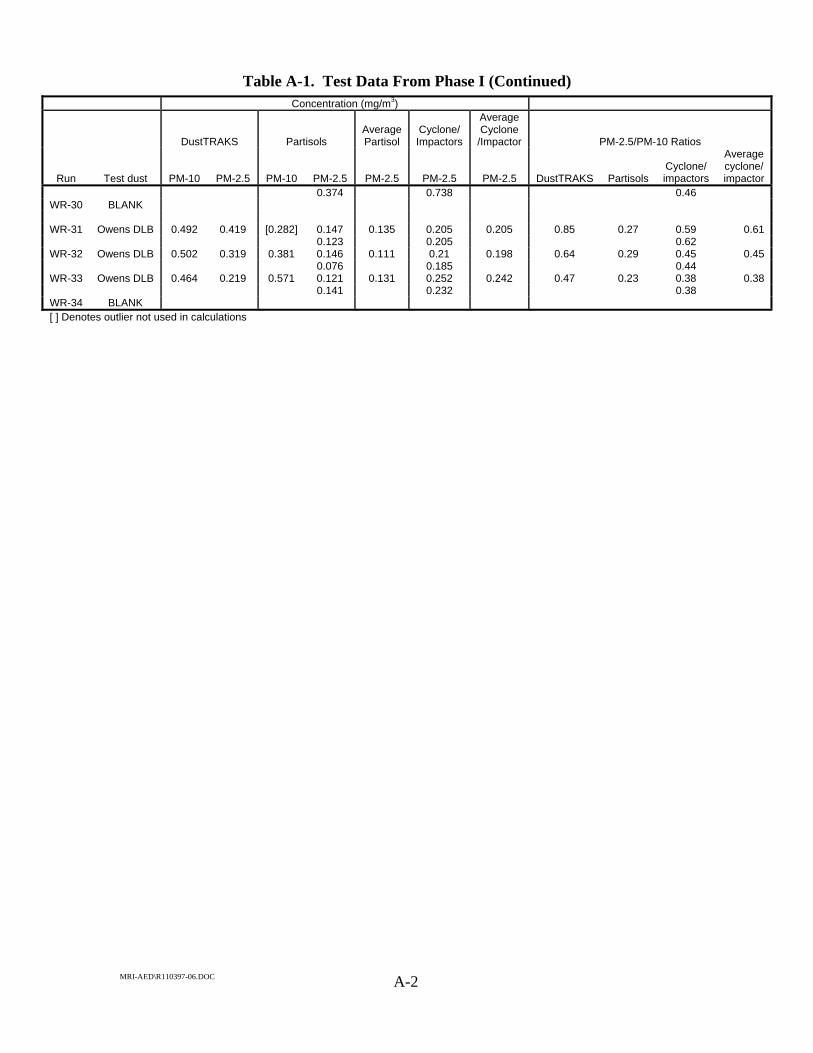
Table A-1. Test Data From Phase I (Continued) Concentration (mg/m3)

DustTRAKS Partisols Average Partisol

Cyclone/ Impactors

Average Cyclone

/Impactor PM-2.5/PM-10 Ratios

Run Test dust PM-10 PM-2.5 PM-10 PM-2.5 PM-2.5 PM-2.5 PM-2.5 DustTRAKS Partisols Cyclone/ impactors

Average cyclone/ impactor

0.374 0.738 0.46 WR-30 BLANK

WR-31 Owens DLB 0.492 0.419 [0.282] 0.147 0.135 0.205 0.205 0.85 0.27 0.59 0.61

0.123 0.205 0.62 WR-32 Owens DLB 0.502 0.319 0.381 0.146 0.111 0.21 0.198 0.64 0.29 0.45 0.45

0.076 0.185 0.44 WR-33 Owens DLB 0.464 0.219 0.571 0.121 0.131 0.252 0.242 0.47 0.23 0.38 0.38

0.141 0.232 0.38 WR-34 BLANK [ ] Denotes outlier not used in calculations


Table A-2. Test Data From Phase II

DustTRAKS Partisol concentration Average of Partisols PM-2.5/PM-10 ratios

Run Test dust PM-10 PM-2.5 A (PM-2.5) B (PM-2.5) C (PM-10) D (PM-10) PM-10 PM-2.5 DustTRAKS Partisols WR-35 AZ Ag Field 0.995 0.241 0.19 0.18 0.927 0.926 0.927 0.185 0.242 0.200

WR-36 AZ Ag Field 0.975 0.247 0.189 0.198 0.883 0.866 0.875 0.194 0.253 0.221

WR-37 AZ Ag Field 1.050 0.262 0.189 0.211 1.723 0.899 1.311 0.200 0.250 0.153

WR-38 AZ Ag Field 2.970 0.720 0.433 0.408 2.752 2.6 2.676 0.421 0.242 0.157

WR-39 AZ Ag Field 3.130 0.631 0.439 0.43 3.501 2.991 3.246 0.435 0.202 0.134

WR-40 AZ Ag Field 2.600 0.738 0.433 0.433 2.514 2.431 2.473 0.433 0.284 0.175

WR-41 AZ Ag Field 4.950 1.030 0.579 0.605 5.548 4.847 5.198 0.592 0.208 0.114

WR-42 AZ Ag Field 5.130 1.580 0.974 0.968 4.694 4.458 4.576 0.971 0.308 0.212

WR-43 AZ Ag Field 5.150 1.650 1.054 1.126 5.124 4.581 4.853 1.090 0.320 0.225

WR-44 BLANK

WR-48 Knik River Sediment 4.010 1.460 0.433 0.451 3.746 3.571 3.659 0.442 0.364 0.121


WR-50 BLANK





WR-55 BLANK

WR-56

Las Cruces Landfill Road 4.980 1.060 0.676 0.662 5.893 5.722 5.808 0.669 0.213 0.115

WR-57


WR-58


WR-59


WR-60


WR-61 BLANK


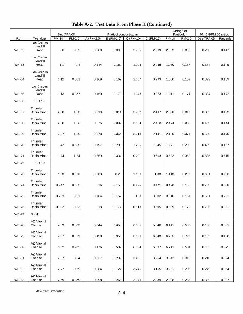
Table A-2. Test Data From Phase II (Continued)


Run Test dust PM-10 PM-2.5 A (PM-2.5) B (PM-2.5) C (PM-10) D (PM-10) PM-10 PM-2.5 DustTRAKS Partisols

WR-62


WR-63


WR-64


WR-65


WR-66 BLANK

WR-67 Thunder Basin Mine 2.58 1.03 0.319 0.314 2.702 2.497 2.600 0.317 0.399 0.122





WR-72 BLANK





WR-77 Blank

WR-78 AZ Alluvial Channel 4.69 0.893 0.344 0.656 6.335 5.946 6.141 0.500 0.190 0.081







Table A-2. Test Data From Phase II (Continued)


Run Test dust PM-10 PM-2.5 A (PM-2.5) B (PM-2.5) C (PM-10) D (PM-10) PM-10 PM-2.5 DustTRAKS Partisols


WR-85 Blank



WR-88 Blank

WR-89 Radium Springs 2.75 1.04 0.338 [-0.122] 2.728 2.483 2.606 0.338 0.378 0.130

WR-90 Radium Springs 2.75 1.06 0.321 0.315 2.514 2.179 2.347 0.318 0.385 0.136

WR-91 Radium Springs 3.05 0.883 [-0.096] 0.238 2.874 2.982 2.928 0.238 0.290 0.081

WR-92 Blank

WR-93 Salton Sea 1.57 0.823 0.163 0.202 0.846 0.765 0.806 0.183 0.524 0.227

WR-94 Salton Sea 1.12 0.605 0.119 0.123 0.628 0.561 0.595 0.121 0.540 0.204

WR-95 Salton Sea 1.17 0.697 0.195 0.18 0.581 0.515 0.548 0.188 0.596 0.342

WR-96 Blank

WR-97 AZ Ag Field 4.83 0.96 0.521 0.627 5.725 5.224 5.475 0.574 0.199 0.105

WR-98 AZ Ag Field 5.42 1.05 0.694 0.746 7.264 6.91 7.087 0.720 0.194 0.102

WR-99 AZ Ag Field 5.1 1.08 0.61 0.673 5.846 5.36 5.603 0.642 0.212 0.114

WR-100 Blank


Table A-3. Field Blank Corrections

Phase 1 Filter type Blank correction Comments 8 X 10 in –0.143 4 X 5 ina 0.040 47 mm –0.053

An overall blank correction was applied to each filter type

in Phase 1

Phase 2 Runs Blank correction WR-35 to 43 0.044 WR-45 to 50 0.044 WR-51 to 54 0.008 WR-56 to 60 –0.002

Only 47-mm filters were used in Phase 2 of testing

WR-62 to 65 –0.004 WR- 67 to 71 0.013 WR-73 to 76 –0.031 WR-78 to 85 0.002 WR-86 to 87 0.007 WR-89 to 92 0.044 WR-93 to 95 0.035 WR 97 to 99 0.033

a Impactor substrate.


Appendix B QA/QC Activities

MRI-AED\R110397-06.DOC

B.1 QA/QC Procedure

The Quality Assurance Project Plan (QAPP) prepared for this test program is a separate document that describes all the QA/QC activities for the project. An outline of that document is attached to the end of this section. B.2 QA/QC Activities

As part of the QA program for this study, audits of sampling and analysis procedures were performed. The purpose of the audits was to demonstrate that measurements are made within acceptable control conditions for particulate source sampling and to assess the source testing data for precision and accuracy. Examples of items audited included gravimetric analysis, flow rate calibration, data processing, and concentration calculation. The mandatory use of specially designed reporting forms for sampling and analysis data obtained in the field and laboratory aided in the auditing procedure.

Requirements for high-volume (hi-vol) sampler flow rates rely on the use of secondary and primary flow standards. The Roots meter is the primary volumetric standard and the BGI orifice is the secondary standard for calibration of hi-vol sampler flow rates. The Roots meter is calibrated and traceable to a NIST standard by the manufacturer. The BGI orifice is calibrated against the primary standard on an annual basis. Before going to the field, the BGI orifice is first checked to assure that it has not been damaged. In the wind tunnel laboratory, the orifice is used to calibrate the flow rate of each hi-vol sampler Table B-1 specifies the frequency of calibration and other QA checks regarding air samplers.

A second pretest activity is the preparation of the hi-vol filters for use in the testing. In this preparation, the filters are weighed under stable temperature and humidity conditions. After they are weighed and have passed audit weighing, the filters are packaged for shipment to the field. Table B-2 outlines the general requirements for conditioning and weighing sampling media. Note the audit weighing is performed by a second, independent analyst.

MRI-AED\R110397-06.DOC B-1

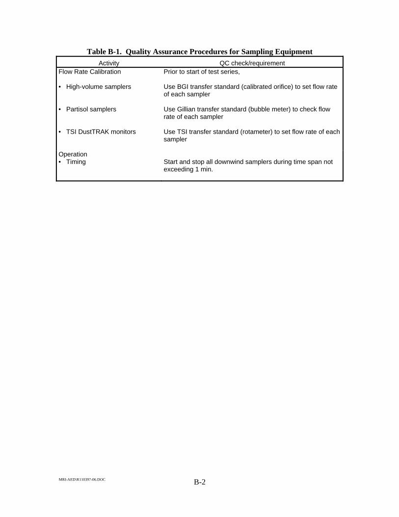
Table B-1. Quality Assurance Procedures for Sampling Equipment

Activity QC check/requirement Flow Rate Calibration • High-volume samplers • Partisol samplers • TSI DustTRAK monitors

Prior to start of test series, Use BGI transfer standard (calibrated orifice) to set flow rate of each sampler Use Gillian transfer standard (bubble meter) to check flow rate of each sampler Use TSI transfer standard (rotameter) to set flow rate of each sampler

Operation • Timing

Start and stop all downwind samplers during time span not exceeding 1 min.


Table B-2. Quality Assurance Procedures for Sampling Media Activity QA check/requirement

Preparation Inspect and imprint glass fiber media with identification numbers.

Conditioning Equilibrate media for 24 h in clean controlled room with relative humidity of 40% (variation of less than ±5% RH) and with temperature of 23°C (variation of less than ±1°C).

Weighing Weigh hi-vol back-up filters to nearest 0.05 mg. Weigh Partisol filters to nearest 0.001 mg. Weigh cascade impactor substrates to nearest 0.05 mg.

Auditing of weights Independently verify final weights of all filters and substrates. Reweigh entire batch if weights of any hi-vol filters deviate by more than ±2.0 mg. For tare weights, conduct a 100% audit by a second analyst. Reweigh any high-volume filter whose weight deviates by more than ±1.0 mg. Follow same procedures for impactor substrates used for sizing tests. Audit limits for impactor substrates are ±1.0 and ±0.5 mg for final and tare weights, respectively.

Correction for handling effects Weigh and handle at least one blank for each 1 to 10 filters of each type used to test.

Calibration of balance Balance to be calibrated once per year by certified manufacturer’s representative. Check prior to each use with laboratory Class S weights.

As indicated in Table B-2, a minimum of 10% field blanks were collected for QC purposes. This involves handling at least one blank filter for every 10 exposed filters in an identical manner to determine systematic weight changes due to handling steps alone. These changes are used to mathematically correct the net weight gain due to handling. A field blank filter is loaded into a sampler and then immediately recovered without any air being passed through the media. Blanks have been successfully used in many MRI programs to account for systematic weight changes due to handling.

After the particulate matter samples and blank filters are collected and returned from the field, the collection media are placed in the gravimetric laboratory and allowed to come to equilibrium. Each filter is weighed, allowed to return to equilibrium for an additional 24 h, and then all of the exposed filters are reweighed by a second analyst. If a filter fails the audit criterion, the entire lot will be allowed to condition in the gravimetric laboratory an additional 24 h and then reweighed. The tare and first weight criteria for filters (Table B-2) are based on an internal MRI study conducted in the early 1980s to evaluate the stability of several hundred 8- x 10-in glass fiber filters used in exposure profiling studies.


B.3 QA/QC Checks for Data Reduction and Validation

Whenever practical, all data collected in the study were entered directly onto standard data forms. All data were recorded on standard data forms using permanent black ink and signed/dated by sampling personnel. Data forms were inspected for completeness and accuracy by the appropriate field supervisor at the end of each test. At that time, data forms were grouped by test number and bound into 3-ring binders.

The data analysis procedures that were used for this project are procedures that have been through several layers of validation in substantiating the performance of the method. It should be noted that blank-corrected sample mass is considered quantifiable (and usable for concentration calculation) only if it equals or exceeds three times the standard deviation of the average net weight change of the field blanks.

An independent auditor performed a check of the calculations in the computer data reduction programs. The Field Team Leader or his/her designee conducted an on-site spot check to ensure that data were being recorded accurately. After the field test, an independent auditor checked data input to assure accurate transfer of the raw data.

For this project, all records were evaluated for the adherence to all procedures and requirements. The items that were reviewed include:

• Gravimetric audit weighing for the assessment of the particulate data, • Calibration and calibration criterion checks, • The results of all blanks, and • The validation of data process systems or procedures.

Selected data were reconstructed, including tracing the calibration back to the

primary standards. Any software (spreadsheets) used to determine numerical values was checked by hand calculating all intermediate and final results for one run by referring to original sources of data (i.e., field filter logs, filter weight logs, run sheets, sampler look-up tables). B.4 Sample Identification and Traceability

To maintain sample integrity, the following procedures were used:

• Each filter was issued a unique identification number. MRI SOP EET-610 describes the numbering system that is employed to identify filter type, project, and other information.

• The sample number was recorded in a sample logbook along with the date the sample was obtained. The sample number was coded to indicate the sample location and test series.


• Other pertinent information that was recorded included short descriptions of

sample type or location, storage location, condition of sample, any special instructions, and signatures of personnel who received the sample for analysis.

• In order to conduct traceability, all sample transfers were recorded in a notebook or on forms. The following information was recorded: the assigned sample codes, date of transfer, location of storage site, and the name of the person initiating and accepting the transfer.

All documented work was reviewed by the project leader for completeness. The

field technical coordinator was responsible for assuring that all samples are accounted for and that proper traceability/tracking procedures were followed.


analysis of the fine fraction of particulate matter in ... · particulate matter in fugitive dust...

Documents