Kaunas University of Technology

Faculty of Electrical and Electronics Engineering

Analysis of Energy Storage in the Electrical Grid:

Optimization for Microgrid and Frequency Containment

Reserve Usage

Master’s Final Degree Project

Felipe Fregoso

Project author

Prof. Saulius Gudžius

Supervisor

Kaunas, 2021

Kaunas University of Technology

Faculty of Electrical and Electronics Engineering

Analysis of Energy Storage in the Electrical Grid:

Optimization for Microgrid and Frequency Containment

Reserve Usage

Master’s Final Degree Project

Electrical Power Engineering (6211EX010)

Felipe Fregoso

Project author

Prof. Saulius Gudžius

Supervisor

Assoc. Prof. Jonaitis Audrius

Reviewer

Kaunas, 2021

Kaunas University of Technology

Faculty and Electrical and Electronics Engineering

Felipe Fregoso

Analysis of Energy Storage in the Electrical Grid: Optimization for Microgrid

and Frequency Containment Reserve Usage

Declaration of Academic Integrity

I confirm the following:

1. I have prepared the final degree project independently and honestly without any violations of

the copyrights or other rights of others, following the provisions of the Law on Copyrights and

Related Rights of the Republic of Lithuania, the Regulations on the Management and Transfer of

Intellectual Property of Kaunas University of Technology (hereinafter – University) and the ethical

requirements stipulated by the Code of Academic Ethics of the University;

2. All the data and research results provided in the final degree project are correct and obtained

legally; none of the parts of this project are plagiarised from any printed or electronic sources; all the

quotations and references provided in the text of the final degree project are indicated in the list of

references;

3. I have not paid anyone any monetary funds for the final degree project or the parts thereof

unless required by the law;

4. I understand that in the case of any discovery of the fact of dishonesty or violation of any

rights of others, the academic penalties will be imposed on me under the procedure applied at the

University; I will be expelled from the University and my final degree project can be submitted to the

Office of the Ombudsperson for Academic Ethics and Procedures in the examination of a possible

violation of academic ethics.

Felipe Fregoso

Confirmed electronically

Fregoso, Felipe. Analysis of Energy Storage in the Electrical Grid: Optimization for Microgrid and

Frequency Containment Reserve Usage. Master's Final Degree Project / supervisor Prof. Dr. Saulius

Gudžius; Faculty and Electrical and Electronics Engineering, Kaunas University of Technology.

Study field and area (study field group): electrical engineering, engineering science.

Keywords: battery, microgrid, frequency control, ancillary service, energy storage.

Kaunas, 2021. 51 p.

Summary

Energy storage is expected to have a larger responsibility in the future of the electrical grid due to the

increase in renewable energy sources that have variable generation. In this thesis, energy storage‘s

role in the electrical grid is discussed along with its economic viability based on its current costs. The

different methods of storing energy are beneficial for different responsibilities in the grid. Ancillary

service markets are changing their requirements to allow energy storage to enter the market. Two

separate simulations were created in this project to analyze how batteries perform financially during

their lifetime.

The first simulation is an optimization model that finds the best sizing for a PV and battery microgrid

system that has the lowest cost over a 12-year period. The model uses a load profile and solar

irradiation data to calculate how much power is produced by the PV and how much load is consumed

each hour. The battery in this model is used as an energy reserve to support the PV when it does not

produce enough power to support the load instead of purchasing power from the main grid. The

simulation uses the particle swarm optimization model where each position of a particle represents a

PV and battery sizing value. The optimization model can find the solution at a much faster speed than

iterating through each possible sizing. The simulation found that batteries are not justified in their use

as the optimal solution only included PV capacity. The price of the BESS system is too expensive

today compared the low prices of purchasing power from the main grid.

The frequency reserve ancillary service market was simulated to analyze if it would be profitable for

a BESS provider to enter the market. Some TSOs have altered their market and it has caused many

BESS providers to participate in the frequency reserve service. Lithuania is in the planning process

of creating a frequency reserve market along with the other Baltic countries and specifications from

their proposed market along with data from already existing markets in continental Europe was used

for the model. There are 3 different services that are expected in the future market and the fastest

service (FCR) is expected to have the most profitability for a BESS. The model uses a BESS to either

charge or discharge its power depending on the frequency deviation of the grid to provide its service

over a 16-year period. Different sizes for the BESS energy capacity and bid capacity were simulated,

but none of them were deemed a good investment at the end of the simulation. The speculated battery

prices by 2030 could make it possible for frequency response service with BESS to be a viable

investment in the future.

Fregoso, Felipe. Energijos kaupiklių elektros tinkle tyrimas: mikrotinklo optimizavimas ir

pritaikymas dažnio palaikymo rezervui. Magistro baigiamasis projektas / vadovas prof. dr. Saulius

Gudžius; Kauno technologijos universitetas, Elektros ir elektronikos fakultetas.

Studijų kryptis ir sritis (studijų krypčių grupė): elektros inžinerija, inžinerijos mokslai.

Reikšminiai žodžiai: baterija, mikrotinklas, dažnio valdymas, papildoma paslauga, energijos

kaupimas.

Kaunas, 2021 p.51

Santrauka

Tikimasi, kad ateityje už energijos saugojimą bus prisiimta didesnė atsakomybė už elektros tinklą dėl

padidėjusių atsinaujinančių energijos šaltinių, kurie gamina kintamą energiją. Šiame straipsnyje

aptariamas energijos kaupimo vaidmuo elektros tinkle ir jo ekonominis gyvybingumas, atsižvelgiant

į dabartines išlaidas. Skirtingi energijos kaupimo metodai yra naudingi skirtingoms atsakomybėms

tinkle. Pagalbinių paslaugų rinkos keičia savo reikalavimus, kad į rinką galėtų patekti energijos

kaupimas. Šiame projekte buvo sukurtos dvi atskiros simuliacijos, skirtos išanalizuoti, kaip baterijos

veikia finansiškai per savo gyvenimą.

Pirmasis modeliavimas yra optimizavimo modelis, kuris nustato geriausią PV ir akumuliatoriaus

mikrogrido sistemos dydį, kurio sąnaudos per 12 metų yra mažiausios. Modelis naudoja apkrovos

profilį ir saulės spinduliuotės duomenis, kad apskaičiuotų, kiek energijos pagamina PV ir kiek

apkrovos suvartojama kiekvieną valandą. Šio modelio baterija naudojama kaip energijos rezervas,

palaikantis PV, kai jis negamina pakankamai energijos, kad palaikytų apkrovą, o ne perkamą galią iš

pagrindinio tinklo. Modeliuojant naudojamas dalelių būrio optimizavimo modelis, kuriame kiekviena

dalelės padėtis atspindi PV ir akumuliatoriaus dydžio vertę. Optimizavimo modelis gali rasti

sprendimą daug greičiau, nei kartojant kiekvieną galimą dydį. Modeliuojant nustatyta, kad baterijos

nėra pateisinamos, nes optimalus sprendimas apima tik PV talpą. BESS sistemos kaina šiandien yra

per brangi, palyginti su žemomis perkamosios galios iš pagrindinio tinklo kainomis.

Buvo imituojama dažnio rezervo pagalbinių paslaugų rinka, siekiant išanalizuoti, ar BESS teikėjui

būtų pelninga patekti į rinką. Kai kurie perdavimo sistemos operatoriai pakeitė savo rinką ir tai

paskatino daugelį BESS teikėjų dalyvauti dažnio rezervo tarnyboje. Lietuva planuoja dažnių rezervo

rinkos kūrimą kartu su kitomis Baltijos šalimis, o modeliui buvo naudojami jų siūlomos rinkos

specifikacijos bei duomenys iš jau esamų žemyninės Europos rinkų. Yra 3 skirtingos paslaugos, kurių

tikimasi būsimoje rinkoje, ir tikimasi, kad greičiausia paslauga (FCR) turės didžiausią BESS

pelningumą. Modelis naudoja BESS arba įkrauti, arba iškrauti savo galią, atsižvelgiant į tinklo dažnio

nuokrypį, kad galėtų teikti savo paslaugą per 16 metų. Buvo imituojami skirtingi BESS energijos

pajėgumų ir pasiūlymų pajėgumų dydžiai, tačiau modeliavimo pabaigoje nė vienas iš jų nebuvo

laikomas gera investicija. Spekuliuojamos akumuliatorių kainos iki 2030 m. Sudarys galimybę BESS

dažnio atsako paslaugai tapti perspektyvia investicija ateityje.

Table of Contents

List of Figures .................................................................................................................................... 1

List of Tables ...................................................................................................................................... 2

List of Abbreviations ......................................................................................................................... 3

Introduction ....................................................................................................................................... 4

1. Review of Energy Storage and its Role in the Grid .................................................................... 6

2. Microgrid Optimization for PV and BESS ............................................................................... 12

2.1 Microgrid Overview .................................................................................................................... 12

2.2 Optimization Model ..................................................................................................................... 13

2.3 Load and Grid .............................................................................................................................. 13

2.4 PV Panels ..................................................................................................................................... 15

2.5 Battery Storage ............................................................................................................................ 16

2.6. Cost Function .............................................................................................................................. 18

2.7 Particle Swarm Optimization Model ........................................................................................... 18

2.8 Results of Simulation .................................................................................................................. 21

2.9 Microgrid Optimization Conclusion ............................................................................................ 22

3. Frequency Reserve Market Analysis ......................................................................................... 23

3.1 FCR Market Process .................................................................................................................... 23

3.2 Battery Degradation ..................................................................................................................... 26

3.3 FCR Model .................................................................................................................................. 26

3.4 BESS System Specifications ....................................................................................................... 27

3.5 Frequency and Market Data ........................................................................................................ 30

3.6 Costs Calculation ......................................................................................................................... 33

3.7 Algorithm of Model ..................................................................................................................... 33

3.8 Results ......................................................................................................................................... 36

3.9 FCR Conclusion .......................................................................................................................... 37

Conclusion ........................................................................................................................................ 39

References......................................................................................................................................... 41

1

List of Figures

Fig. 1.1. Energy storage power capacity shares by main-use case and technology group .................. 7

Fig. 1.2. Lithium-Ion battery charging and discharging process ........................................................ 8

Fig. 1.3. USA large-scale battery applications in 2018 ....................................................................... 9

Fig. 1.4. PEV integration into the grid [21]....................................................................................... 10

Fig. 2.1.1. Schematic of Microgrid ................................................................................................... 12

Fig 2.2.1. Microgrid overview for simulation ................................................................................... 13

Fig. 2.3.1. Load profile of winter day ............................................................................................... 14

Fig. 2.3.2 Load profile of summer day .............................................................................................. 14

Fig. 2.4.1. Solar Irradiation of Winter day in Kaunas ....................................................................... 15

Fig. 2.4.2: Solar Irradiation of Summer day in Kaunas .................................................................... 16

Fig. 2.5.1. BESS Energy Capacity throughout a day ........................................................................ 17

Fig. 2.7.1. Particle Swarm Optimization convergence ...................................................................... 19

Fig. 2.7.2. PSO algorithm .................................................................................................................. 20

Fig. 2.7.3. Cost calculation flow chart .............................................................................................. 21

Fig. 3.1.1. Balancing market process for frequency restoration ....................................................... 23

Fig. 3.1.2. FCR activation by frequency deviation ........................................................................... 24

Fig. 3.1.3. Overfulfillment and deadband operation degrees of freedom ......................................... 25

Fig. 3.4.1. Permitted operating SOC range of BESS system ............................................................ 27

Fig. 3.4.2. SOC during one day for BESS model and adjusted for RFC .......................................... 28

Fig. 3.4.3. Battery cycles before 70% EOL capacity for DOD of cycle ........................................... 29

Fig. 3.4.4: Cycles for different DOD in a year for 1MW/2MWh BESS........................................... 30

Fig. 3.5.1. Grid frequency measurements over 2-year period ........................................................... 31

Fig. 3.5.2. Probability of Grid Frequency over 2-year period ........................................................... 31

2

List of Tables

Table 1.1.1. Technical and economical characteristics of ESS .......................................................... 8

Table 2.6.1. Simulation prices .......................................................................................................... 18

Table 3.3.1: FCR specifications........................................................................................................ 26

Table 3.6.1. Costs for model simulation calculation ........................................................................ 33

Table 3.7.1: Efficiencies for SOC calculation .................................................................................. 34

Table 3.8.1: FCR simulation results ................................................................................................. 36

Table 3.8.2. Analysis of hypothetical prices to achieve 0 NPV ....................................................... 37

3

List of Abbreviations

BESS - battery energy storage system

CAISO - California Independent System Operator

DG - distributed generation

DER - distributed energy resource

DOD - depth of discharge

ENTSO-E - European Network of Transmission System Operators for Electricity

EOL - end of life

ESS - energy storage system

FCR - frequency containment reserve

GA - generic algorithm

LFP - lithium iron phosphate battery

NPV - net present value

PJM - Pennsylvania, Michigan, New Jersey transmission system operator

PSO - particle swarm optimization

PEV - plug-in electric vehicle

PV - photovoltaic

RES - renewable energy source

RFC - rain flow counting algorithm

RTE - Réseau de Transport d'Électricité

SOC - state of charge

TSO - transmission system operator

VRFB - vanadium redox flow battery

4

Introduction

Renewable energy has continued to increase as a source generation in electrical grids throughout the

world due to government policy aimed to greener technologies and decarbonization objectives of the

future grid. The renewable energy sources that expect the largest increase in generation share are

solar and wind power which both have variable generation and it makes it difficult to predict the

amount of power that they will produce each day [1]. Although there has been debate about the

structure of the future grid that can properly suite RES technologies, energy storge is expected have

an important role in the future grid regardless of the structure used [2]. Energy storage will allow the

grid to maintain resiliency and reliability as renewable energy integration increases. It can be used as

a secondary power storage in scenarios where DG is not able to provide sufficient power and can

work congruently with the load and DG to operate a microgrid.

One of the problems associated with integrating energy storage into the electrical grid, is that it is

difficult to justify the price associated with the investment of energy storage [3]. Apart from its role

as a secondary energy reserve, an ESS can also participate in the ancillary service markets to earn

money for its services. There are a variety of ways in which energy storage can already be used in

grid by providing ancillary services. There are also different energy storage technologies that are best

suited to provide different services to the grid. This thesis will analyze different methods in which

energy storage is used in the grid and simulate two methods to assess their financial viability. The

objective of this thesis to measure the performance of battery storage in the grid to see if it is

economically viable today given its current prices. A BESS is measured performing two different

functions in this work, an energy reserve in a grid-connected microgrid, and primary frequency

control in the frequency control ancillary service market.

The microgrid that is simulated in this thesis consists of a PV providing the DG for the microgrid, a

BESS that stores power as a reserve, the load that consumes power in the microgrid, and the main

grid that works congruently with the microgrid. The objective of this section is:

1. Create a model that finds the optimal sizing of the PV and BESS of the microgrid that gives

the lowest cost of operation over a 12-year period.

2. Analyze the optimal sizing solution and compare with a consumer that only purchases power

from the main grid to check if DG from PV with a BESS is competitive at today’s prices.

The particle swarm optimization method is used to converge to the optimal size of batteries and PV

that should be used. Solar irradiation data is used to calculate the amount of power that can be

produced at each hour by the number of PVs that are used, and a load profile of hourly data calculates

the load at each hour. If there is excess power produced by the PV system compared to the consumed

load, the excess power can be used to charge the BESS. If there is not enough power produced by the

PV system, energy stored by the BESS is used to compensate the difference. Power is purchased from

the main grid in a scenario where the PV and BESS cannot provide the sufficient power to the load.

The grid costs along with the costs associated with the microgrid are added together over the 12-year

period as the model iterates through different sizes to find the lowest cost.

The frequency control service model consists of a BESS that provides fast frequency control reserve

for the grid based on the specifications of Lithuania’s upcoming implementation of a frequency

control market. The objective of this section is:

5

1. Create a model with a BESS that provides FCR service based on the specifications of

Lithuania’s future market.

2. Analyze whether it is profitable for a BESS to participate in the new frequency control market

by modelling different bid sizes with different energy capacities of the BESS.

The BESS must give a symmetrical bid in the up and down direction when providing its service. If

the frequency of the grid is higher than 50 Hz, the BESS must charge proportional to the deviation to

help reduce the high frequency level. If the frequency of the grid is below 50 Hz, the BESS must

discharge proportional to the deviation to help increase the system frequency. A time series of

frequency data with values at every 10 seconds is used to calculate the action that the BESS should

perform. Different sizes for the power and energy capacity are simulated over a 16-year period to

check the net present value of the investment, the degradation of the BESS over that period, and the

reliability at which BESS could perform the service.

6

1. Review of Energy Storage and its Role in the Grid

There are a variety of technologies currently used on the grid to carry out different responsibilities.

Figure 1.1 [4] shows a graph of how different energy storage methods are used to perform different

functions on the grid that best fit their characteristics. Pumped hydro storage is a mature energy

storage method that has a large capacity already in use throughout the world. It can use the potential

energy of large reserves of water to create electricity during peak pricing hours while using electricity

to pump water back up the reserve in times of low electricity pricing. This makes it very useful as an

electrical capacity supply that that can be operated in times of high load demand. The technology is

limited to the available land and water and it also needs 10 to 15 minutes of reaction time to provide

power [5]. This limitation does not allow this system to be used for capabilities that require a fast

response time.

Other electromechanical technologies are also used as an electricity supply but are used more for the

purpose of on-site power or a black start. Flywheels use angular momentum to store power as kinetic

energy. They have high power and energy density that makes them useful for stabilizing system

voltage or frequency. They essentially have an infinite number of charge and discharge cycles and

require less maintenance over their lifetime compared to chemical batteries. The disadvantage to

Flywheel technology is that they have up to 20% self-discharge per hour in their stored capacity and

they are very sensitive to any shocks that could disrupt their rotation and affect the overall system

[6]. Compressed air storage is an electromechanical storage method that uses gas pressure with

compression of air in a reservoir to convert it into a modified gas. The compressed modified gas is

expanded to rotate a turbine coupled with a generator for producing electricity [7]. They can be used

to serve a large capacity when built with an underground reservoir to hold the compressed air. They

can also be built at a smaller scale above ground in storage tanks. The disadvantage to the system on

a large scale, is the need for land to hold a large underground reservoir. There is also a need to pay

for the gas that will be used in the process of compressing the air [8].

Electrochemical storage is the common method of energy storage when thinking of a traditional

battery system. It involves using a chemical reaction in the batteries cell to release electrons and cause

the flow of electricity. An emerging technology that could be important in the future of energy storage

is vanadium redox flow batteries. They use an electrolyte storage system in which the electrolytes

will participate in either reduction or oxidation reactions creating free electrons and causing the flow

of electricity. They have very low storage losses and can operate for many lifecycles. Since VRFB is

in its early phase as a commercial product, electrolyte materials are still costly and it does not have a

very high energy density [9]. There will need to be significant reduction in the electrolyte cost of

VRFB for it to be competitive with other battery systems currently used in the grid.

7

Fig. 1.1. Energy storage power capacity shares by main-use case and technology group [4]

Two commonly used batteries for storage in the grid are lead-acid batteries and lithium-ion batteries.

Compared to lithium-ion batteries, lead-acid batteries are a cheaper alternative for energy storage.

Alternatively, lithium-ion batteries have much higher energy density and can go through many more

life cycles [10]. The cathode and anode of the battery hold lithium and the electrolyte can carry

positive lithium ions through the separator from one side to another depending on whether the battery

is charging or discharging. When there is connection of a circuit on both sides of the battery, the free

electron can flow across the circuit since it is attracted to the positive lithium ion moving across the

separator thus creating a current as seen in Figure 1.2 [11]. The fast response of lithium-ion batteries

makes them a great candidate for primary frequency response in the grid. When there is a deviation

from the permitted frequency in the main grid, there needs to be sources that can quickly absorb or

deliver power to help get the frequency back to an adequate level. In [12], control strategies were

made to see how to optimize the charging and discharging of lithium ion batteries to be used in

frequency response.

As discussed previously, there are different characteristics to each energy storage technology that

makes them advantageous for different functions. Lifetime, cost, energy density, and overall

efficiency of the system are all things that should be weighed when deciding on the proper energy

storage system for the needed function. In [13], there is a Table of different energy storage

technologies highlighting their specific characteristics.

8

Fig. 1.2. Lithium-Ion battery charging and discharging process [11]

Table 1.1.1. Technical and economical characteristics of ESS [13]

ESS

Tehcnlogy

Power Range

(MW)

Energy

Density

(Wh/kg)

Power

density

(W/kg)

Discharge

time

Response

time

Round trip

eff. (%)

Flywheel 0.01-0.25 5-80 700-1200 sec – 15 min sec 90-95

Compressed

air above

ground

3-15 140 – 300 bar - 2 – 4 hrs sec-min 70-90

Lead-Acid <20 30 – 50 200 – 400 sec – 5 hrs ms 70-90

Lithium-ion 0.05-100 120 – 230 150 – 2k min – 1hr ms 85-95

VRFB 0.01 – 10 65 – 75 - 8 – 10 hrs ms 60 – 80

A common way to earn money with energy storage on the grid today, is through ancillary services.

Ancillary services are additional services that can be provided to help keep the reliability of the grid,

such as maintaining proper power flow, maintaining balance between the supply and demand, or

recovery in the event of a system failure. TSOs around the world have created different kinds of

ancillary service markets to incentivize providers to supply these services. Some of these markets

have services that can be adequately provided by a BESS and even have regulation that has made it

easier for BESS providers to enter the market.

Large-scale battery capacity has continued to increase every year in the United States as TSOs have

changed their regulations to make it easier for energy storage to participate in their ancillary service

markets [14]. The most notable change came in 2011, when the Federal Energy Regulatory

Commission required TSO markets to provide compensation to resources that can provide faster-

ramping frequency regulation. Frequency regulation services are used to help keep the power system

frequency close to its required operating value. PJM split their frequency regulation market into one

market for fast-ramping services and another for its slower ramping services. The provider bids for a

symmetrical max value of power in MW that they can either supply or absorb from the grid based on

the frequency deviation of the grid. The compensation for the frequency regulation market uses a

pay-for- performance method based on a performance score for the providers. The performance factor

is based on the accuracy at which the expected power can be provided and how quickly the response

can be activated due to a change in the grid frequency. The service is also compensated on its mileage

9

based on the change in power that needs to be provided during the service over the highest capacity

that is bid by the provider in ΔMW/MW [15]. Battery storage can receive a good performance score

because of its fast response properties and their high accuracy with an inverter and charge control

system. The new fast response market attracted many BESS providers and similar changes at other

TSOs around the USA have also introduced more battery storage into the grid. Figure 1.3 [14] shows

that the majority of the battery capacity that has been installed throughout different TSOs has been

for frequency regulation and PJM has the largest capacity due to their fast-response market that made

participation for BESS providers easier.

Fig. 1.3. USA large-scale battery applications in 2018 [14]

As seen in the previous Figure, the gid operator of California (CAISO) has the largest battery energy

capacity of any TSO in the United States. In 2013, a bill was passed in the state of California requiring

utilities to procure more energy storage to increase the reliability of the gid in case of loss in

generation capacity [16]. Some of this capacity is used for the ramping/spinning reserve market since

regulations were changed in CAISO reducing the minimum power capacity for providers from 1 MW

to 500 kW and also reducing the requirement of the service time from 2 hours to 30 minutes [17].

The reduced requirements give easier entry to a BESS provider because they need less investment in

energy capacity of their system to participate. The ramping/spinning reserve market is used to bring

more power into the system in scenarios where there are unexpected losses in generation and the

system must be kept balanced. It is the second-most profitable ancillary service market for batteries

to participate in behind the frequency reserve market. Another way for batteries to earn money is

through arbitrage by charging during periods where electricity is less expensive and then selling the

power back during times when electricity is more expensive, although this is power would be traded

in a real-time market and not an ancillary service market.

California also has the highest use of small-scale battery-storage compared to other locations in the

United States [14]. Most of this battery capacity is directly owned by the utilities with some of the

capacity owned for commercial and residential purposes. These smaller battery systems are mostly

used to support distributed generation of renewable energy sources. The batteries can be used to store

power during times when the RES is producing more power than what is consumed by the local load.

The battery can later be discharged to provide power to the load during times when the RES is not

producing enough power. DG combine with energy storage and a localized load to cooperate in a

10

microgrid. The usage of battery storage with a RES to operate a microgrid is further discussed in

Section 2 of this thesis.

In continental Europe, there are not separate ancillary service markets for frequency reserves and

spinning reserves like in the United States, but it is instead encompassed in one frequency control

market [18]. The services in this market are split up into three parts (primary, secondary, and tertiary

reserves) based on the response time that is needed for the provider. The primary reserve service, also

known as FCR, is usually the most profitable for battery systems because it requires the fastest

response time and is also a symmetrical service needing to either supply or remove power from the

grid. As opposed to the United States, the frequency reserve service in continental Europe is only

paid for the symmetrical capacity it can provide and it is not given a performance score that affects

its payment or a mileage payment for the change in power it needs to provide. This market has been

implemented earlier in different countries while others are still in the planning stages, but battery

storage already been implemented for this service. France is currently in the process of building their

largest BESS to participate in their primary reserve frequency control market and the total capacity

is expected to be 25MW/MWh for an estimated cost of €600/kWh and the BESS is expected to have

a lifetime of 15 years [19, 20]. Battery participation in the frequency control market is further

discussed in Section 4 where a model based on the rules of continental Europe’s primary reserve

service is simulated.

The ancillary service markets like frequency control usually involve systems with large energy

capacities because they take place at the transmission level and require minimum bids of 1 MW in

Europe. There has been research discussion for providing ancillary services with many smaller battery

systems aggregated together that when combined have a large capacity. A potential method of

aggregating battery capacity is though plug-in electric vehicles because they spend most of their time

stationary and could be used to provide ancillary services during the time when the vehicle is not

driven. This new stream of revenue could help reduce the cost of electric vehicles and increase the

amount of electric vehicles on the road [21].

Fig. 1.4. PEV integration into the grid [21]

11

The ancillary service markets need adjustments to allow all the PEVs to participate individually

because of the large capacities that are usually required to bid. A provider like a rental service who

has a large fleet of PEVs could participate individually by having all the vehicles that are not in

service from their fleet connected to the grid. It would be most profitable to have the fleet of unused

cars participate in the fast frequency regulation market [22]. It is important to account for the

uncertainty of whether the vehicle will be stationary and if there is sufficient capacity to provide

service at the expected time. Historical data like driving distances and time can be used to make a

predictive model of available service times and the capacity that can be provided [23].

12

2. Microgrid Optimization for PV and BESS

Electricity generation using fossil fuels has been a topic of much concern for the future due to the

environmental concerns associated with carbon emissions. There have been laws and regulations

around the world to try to reduce fossil fuel generation and in turn increase the amount of electricity

generated by renewable energy resources. Using DG in the electrical grid is one method to increase

renewable energy production. This allows a variety of different sources of energy generation to

produce power without needing a large, centralized source of power production to participate. One

way to manage different distributed energy sources, is through a microgrid. A microgrid can be

defined as, “a group of interconnected loads and distributed energy resources with clearly defined

electrical boundaries that acts as a single controllable entity with respect to the grid and can connect

and disconnect from the grid to enable it to operate in both grid-connected or island modes” [24]. One

of the largest issues with implementing microgrids for real world application is the optimization.

Currently, many microgrid projects carry much financial uncertainty and are not profitable for

investors due to many challenges associated with the planning and designing costs [25]. In this

section, an optimization model is discussed to try to make microgrids financially viable.

2.1 Microgrid Overview

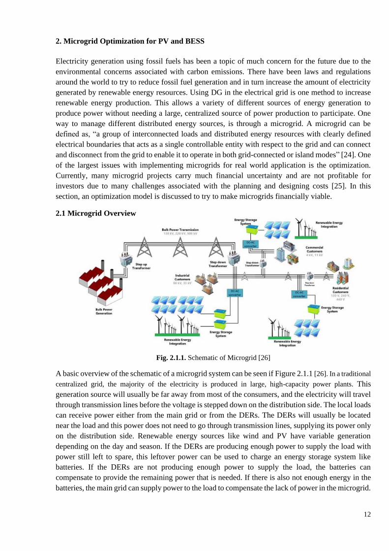
Fig. 2.1.1. Schematic of Microgrid [26]

A basic overview of the schematic of a microgrid system can be seen if Figure 2.1.1 [26]. In a traditional

centralized grid, the majority of the electricity is produced in large, high-capacity power plants. This

generation source will usually be far away from most of the consumers, and the electricity will travel

through transmission lines before the voltage is stepped down on the distribution side. The local loads

can receive power either from the main grid or from the DERs. The DERs will usually be located

near the load and this power does not need to go through transmission lines, supplying its power only

on the distribution side. Renewable energy sources like wind and PV have variable generation

depending on the day and season. If the DERs are producing enough power to supply the load with

power still left to spare, this leftover power can be used to charge an energy storage system like

batteries. If the DERs are not producing enough power to supply the load, the batteries can

compensate to provide the remaining power that is needed. If there is also not enough energy in the

batteries, the main grid can supply power to the load to compensate the lack of power in the microgrid.

13

Some microgrid have the functionality to operate in an “islanded mode” if there is ever a disruption

in the main grid that causes an outage, and the microgrid can disconnect from the main grid and

provide power autonomously to the load. Microgrids can also switch to an “islanded mode” in the

case of scheduled maintenance on the main grid. There can be multiple microgrids connected with

the main grid supplying power to local loads. The microgrid will usually have an energy management

system that will be responsible for making the decision of what mode of operation the microgrid

should be in operation [27]. An “islanded mode” requires more complexity for the control system of

the microgrid and it should be able to supply all the essential load within its area [28]. The complexity

of the system makes it more expensive to operate compared to a grid-connected microgrid, but the

costs may be justified by having continuous reliability for a critical load that should not lose power.

Therefore, this study will only focus on the optimization of grid-connected microgrids due to their

lower cost of implementation and the difficulty to assess the opportunity cost of maintaining power

during an outage.

2.2 Optimization Model

The model created for this optimization project consists of three main pieces and a high-level diagram

of how these pieces interact can be seen in Figure 2.2.1. There is a DG, which consists of solar panels

and batteries for energy storage. The DG is the energy source of this microgrid and the part of the

model that will change size in the optimization process. There is the load that represents the electricity

consumed and it needs to be supplied with sufficient power during all times of the operation. The

main grid can supply electricity to the load in scenarios when the DG does not supply sufficient

energy to power the load. Power can also be transferred over to the main grid in the scenario where

the distributed generation produces excess energy from what is consumed by the load.

Fig 2.2.1. Microgrid overview for simulation

2.3 Load and Grid

The load profile that was used for the calculation came from KTU buildings on Studentų gatvė 48

and 48A. These load profiles were combined and treated as the load for one bus in our system that is

fed by the PV system. The load profile on a winter day in February and a summer day in August can

be seen below. The load consumed throughout the day can have different characteristics depending

on seasonal changes that can influence how electricity is consumed.

14

Fig. 2.3.1. Load profile of winter day

Fig. 2.3.2 Load profile of summer day

15

As seen on the graphs, there is more load consumed on a typical summer day while both Figures

follow a similar load profile shape as the electricity consumption ramps up around the time the school

day begins, and then the consumption begins to fall at around the middle of the day. The average

electricity price paid in Lithuania used for this model is €0.15/kWh [29]. In the model, the peak hours

(8h-16h) were made to have an electricity price of €0.17/kWh and the non-peak hours were made to

have a price of €0.13/kWh. The model was also designed to increase the load by one percent in each

year of operation and to increase the price of electricity by two percent each year.

2.4 PV Panels

Solar irradiation data needed to be collected to find the amount of solar power that could be produced

on a given day. Different literature discussed how the amount of power produced by PV panels can

best be calculated in an optimization problem based on the amount of panels used and the area on

each panel [30, 31]. The equation used in this model was:

𝑃𝑃𝑉(𝑡) = 𝜂 ∙ 𝐸(𝑡) ∙ 𝑁𝑃𝑉 ∙ 𝐴𝑃𝑉 (2.4.1)

If: 𝜂 – conversion efficiency; 𝐸(𝑡) – solar irradiance; 𝑁𝑃𝑉 – number of PV panels; 𝐴𝑃𝑉 – area of a

single PV panel.

The solar irradiance surface data from Kaunas, Lithuania is collected from [32] which uses hourly

satellite data to collect the solar irradiation of Europe [33]. The solar irradiation of a winter day in

February and a summer day in August of Kaunas can be seen below.

Fig. 2.4.1. Solar Irradiation of Winter day in Kaunas

16

As seen from the Figures, the microgrid can produce more power in the summer time compared to

the winter time. There are more hours of sunlight in a summer day and that allows for more hours of

solar irradiation to power the solar panels compared to the winter. The Figures also show that at peak

sunlight hours, almost six times as much solar irradiation is available in the summer compared to the

winter.

Fig. 2.4.2: Solar Irradiation of Summer day in Kaunas

Information about the specifications of the solar panel is collected from [34]. This information is used

to collect solar data for variables needed in the above calculation like panel size and efficiency. It is

also used to collect cost data for the solar panels for the overall system cost calculation. The PV panels

for this simulation each have an area of 1.6 m2and they have an efficiency of 19%. The standard

testing conditions for calculating the rated power of a PV panel use the irradiation value of 1000

W/m2 and using these conditions with Equation 2.4.1 gives a rated capacity power capacity 304 W

for each PV panel.

2.5 Battery Storage

The energy storage system used for this simulation is simulated using the properties of lithium-ion

batteries. Data from [4, 35, 36] is used to find cost characteristics related to installation, maintenance,

and inverter costs associated with lithium ion batteries used to calculated the total cost of the system.

The battery storage can only be used in the simulation if there is sufficient charge for operation. The

current state of charge (SOC) of the battery system needs to be calculated at every time step to keep

track of the current battery state. The state of charge of the battery system can be calculated with:

17

𝑆𝑂𝐶(𝑡) = 𝑆𝑂𝐶(𝑡 − 1) + 𝜂𝐵𝑎𝑡𝑡 ∙ 𝑁𝐵𝑎𝑡𝑡 ∙ ∆𝑃𝐵𝑐ℎ𝑎𝑟𝑔𝑒 𝑑𝑖𝑠𝑐ℎ𝑎𝑟𝑔𝑒⁄ (2.5.1)

If: 𝑆𝑂𝐶(𝑡 − 1) – state of charge from the previous time-step; 𝜂𝐵𝑎𝑡𝑡 – efficiency of the battery

system; 𝑁𝐵𝑎𝑡𝑡 – number of batteries; ∆𝑃𝐵𝑐ℎ𝑎𝑟𝑔𝑒/𝑑𝑖𝑠𝑐ℎ𝑎𝑟𝑔𝑒 – charge or discharge rate of the battery

system.

Depending on whether the system is in a scenario where the batteries will charge or discharge, the

rate will either add or subtract from the previous state of charge. Although lithium-ion batteries have

flexibility in the charge and discharge rate, this simulation uses them as a secondary energy supply,

and they are kept at a constant rate. Charging and discharging batteries at an adequate C-rate can be

beneficial prolonging the battery life [4]. Using the batteries for rapid charge or discharge so that they

are available to be used as an ancillary service is discussed later in Section 3. It should also be noted

that the batteries cannot be charged or discharged beyond their theoretical limits.

𝑆𝑂𝐶𝑚𝑖𝑛 ≤ 𝑆𝑂𝐶(𝑡) ≤ 𝑆𝑂𝐶𝑚𝑎𝑥 (2.5.2)

If: 𝑆𝑂𝐶𝑚𝑖𝑛 – minimum state of charge of battery for operation; 𝑆𝑂𝐶𝑚𝑎𝑥 – maximum state of charge

of battery for operation.

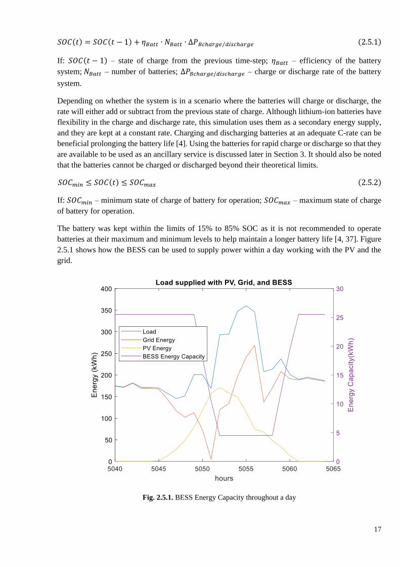
The battery was kept within the limits of 15% to 85% SOC as it is not recommended to operate

batteries at their maximum and minimum levels to help maintain a longer battery life [4, 37]. Figure

2.5.1 shows how the BESS can be used to supply power within a day working with the PV and the

grid.

Fig. 2.5.1. BESS Energy Capacity throughout a day

18

The early hours of the day have no sunlight and the load is supplied completely by the grid. Later in

the day when there are peak grid prices, the battery is discharged so that most of the load is supplied

by the PV and BESS without the help of the grid. After the BESS is out of charge, the load is provided

by the grid and PV system. In the evening once the peak pricing hours are over, the battery is

recharged with the grid and the little PV power that is available.

2.6. Cost Function

The cost function is used to calculate the total cost of the microgrid. This includes all the costs

associated with the purchase, installation, and maintenance of the equipment used in the microgrid

along with the cost of the power consumed from the main grid. The cost function used for this problem

can be seen below:

𝐶𝑛 = 𝐶𝑔𝑟𝑖𝑑 + 𝐶𝑃𝑉 + 𝐶𝐵𝑎𝑡𝑡 (2.6.1)

If: 𝐶𝑛 – total cost calculated; 𝐶𝑔𝑟𝑖𝑑 – cost of the electricity purchased from the grid, 𝐶𝑃𝑉 – cost of the

photovoltaic panels (includes purchase, installation, O&M costs, cost of inverter); 𝐶𝐵𝑎𝑡𝑡 – cost of the

lithium-ion batteries used (includes purchase, installation, O&M costs, cost of inverter).

The price is added up for the 12-year simulation and goal of the optimization function is to reduce

the costs and find the lowest achievable value of 𝐶𝑛. The prices used for the simulation of this system

are summarized below in Table 2.6.1.

Table 2.6.1. Simulation prices

Parameter Cost

Electricity from main grid €0.17/kWh peak/€0.17/kWh non-peak

Investment/installation of BESS €600/kWh

O&M BESS €6/kWh/year

Inverter and battery control €100/kWh

Investment/installation of PV panel

(Area=1.6m2)

€300/panel

PV inverter €25/kW

O&M of PV €33/kW

2.7 Particle Swarm Optimization Model

The goal of the optimization model is to find the optimal number of PV panels and batteries to operate

the microgrid at the lowest cost possible. Methods like fuzzy decision can be used to calculate the

optimal sizing of a microgrid [38]. In [39], it is shown how GA can be used to find the optimal sizing

and location of a grid connected PV system. In [40], it is shown how particle swarm optimization

(PSO) is a much more efficient method of calculating PV sizing when compared to GA. PSO is an

optimization method inspired from the social behavior of biological organisms, like birds that will

flock to a food source with the help of a combination expressing the influence on the position of the

body through the historical positions of itself and its neighbor [41]. PSO was chosen as the

19

optimization model to use in this project because it is simple and robust for implementation, and it

also has an efficient simulation run-time.

Fig. 2.7.1. Particle Swarm Optimization convergence [42]

Particle swarm optimization is based on the location and velocity of each particle in the system. The

equations to calculate the position and location are calculated with:

𝑥𝑘+1𝑖 = 𝑥𝑘

𝑖 + 𝑣𝑘+1𝑖 (2.7.1)

𝑣𝑘+1𝑖 = 𝑤𝑣𝑘

𝑖 + 𝑐1𝑟𝑎𝑛𝑑(𝑝𝑖 − 𝑥𝑘𝑖 ) + 𝑐2𝑟𝑎𝑛𝑑(𝑝𝑘

𝑔− 𝑥𝑘

𝑖 ) (2.7.2)

If: 𝑥𝑘+1𝑖 – the next particle position; 𝑥𝑘

𝑖 – current particle position; 𝑣𝑘+1𝑖 – next calculated particle

velocity; 𝑤 – inertia coefficient; 𝑣𝑘𝑖 – current velocity of the particle; 𝑐1 – personal acceleration

coefficient, 𝑝𝑖 – personal best position of that specific particle; 𝑐2 – global acceleration coefficient,

𝑝𝑘𝑔

– global best position of all the particles.

As seen in Figure 2.7.1 [42], each particle in this algorithm is randomly assigned a position during

the initialization. Each position can then be classified by how well it performs based on the given

criteria. The particle that best fits the criteria is assigned as the global best position upon initialization.

The particles then calculate their velocity with equation 2.7.2. The velocity is influenced by its

previous velocity, the difference of its personal best position and its current position multiplied by a

random variable from zero to one, and the difference of the historic best position of the swarm and

its current position multiplied by a random number zero to one. The velocity is then added to the

previous position to find its new position and then all the particles in the swarm check if their new

position is closer to the criteria. The particles use their best position and the swarm’s best position as

they mor around each iteration as they converge to the solution. The random variable is used to make

all the particles follow different paths to ensure that the proper solution is not missed, and the particles

converge to the incorrect solution. The number of particles that is initialized at the beginning should

be sufficient so that there are random particles in all possible areas that could be the solution because

this could also cause the particles to converge to the incorrect value.

20

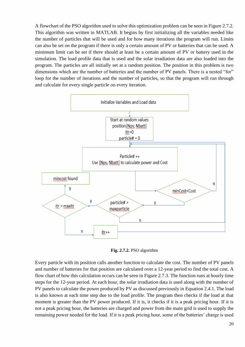
A flowchart of the PSO algorithm used to solve this optimization problem can be seen in Figure 2.7.2.

This algorithm was written in MATLAB. It begins by first initializing all the variables needed like

the number of particles that will be used and for how many iterations the program will run. Limits

can also be set on the program if there is only a certain amount of PV or batteries that can be used. A

minimum limit can be set if there should at least be a certain amount of PV or battery used in the

simulation. The load profile data that is used and the solar irradiation data are also loaded into the

program. The particles are all initially set at a random position. The position in this problem is two

dimensions which are the number of batteries and the number of PV panels. There is a nested “for”

loop for the number of iterations and the number of particles, so that the program will run through

and calculate for every single particle on every iteration.

Fig. 2.7.2. PSO algorithm

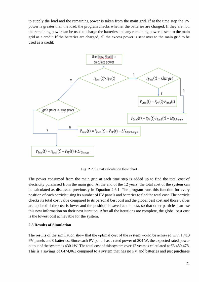
Every particle with its position calls another function to calculate the cost. The number of PV panels

and number of batteries for that position are calculated over a 12-year period to find the total cost. A

flow chart of how this calculation occurs can be seen in Figure 2.7.3. The function runs at hourly time

steps for the 12-year period. At each hour, the solar irradiation data is used along with the number of

PV panels to calculate the power produced by PV as discussed previously in Equation 2.4.1. The load

is also known at each time step due to the load profile. The program then checks if the load at that

moment is greater than the PV power produced. If it is, it checks if it is a peak pricing hour. If it is

not a peak pricing hour, the batteries are charged and power from the main grid is used to supply the

remaining power needed for the load. If it is a peak pricing hour, some of the batteries’ charge is used

21

to supply the load and the remaining power is taken from the main grid. If at the time step the PV

power is greater than the load, the program checks whether the batteries are charged. If they are not,

the remaining power can be used to charge the batteries and any remaining power is sent to the main

grid as a credit. If the batteries are charged, all the excess power is sent over to the main grid to be

used as a credit.

Fig. 2.7.3. Cost calculation flow chart

The power consumed from the main grid at each time step is added up to find the total cost of

electricity purchased from the main grid. At the end of the 12 years, the total cost of the system can

be calculated as discussed previously in Equation 2.6.1. The program runs this function for every

position of each particle using its number of PV panels and batteries to find the total cost. The particle

checks its total cost value compared to its personal best cost and the global best cost and those values

are updated if the cost is lower and the position is saved as the best, so that other particles can use

this new information on their next iteration. After all the iterations are complete, the global best cost

is the lowest cost achievable for the system.

2.8 Results of Simulation

The results of the simulation show that the optimal cost of the system would be achieved with 1,413

PV panels and 0 batteries. Since each PV panel has a rated power of 304 W, the expected rated power

output of the system is 430 kW. The total cost of this system over 12 years is calculated at €3,450,478.

This is a savings of €474,061 compared to a system that has no PV and batteries and just purchases

22

electricity from the main grid. The cost of the BESS was too high to justify energy storage in the

system.

2.9 Microgrid Optimization Conclusion

The program was successful in finding the optimal solution for the lowest cost, but that solution

included no batteries in the system. The price of BESS will need to significantly drop for it to satisfy

its investment in a grid-connected microgrid. In a microgrid with an “islanded mode” the customer

will need to analyze if the benefits of maintaining power to their load when the main grid has an

outage and check if the cost of energy storage is justified.

Energy storage can play an important role in microgrids because it can supply reserve energy quicky

without needing a ramp up time compared to generators. The flexibility and variety of uses that energy

storage can have in power systems will be important for the future of the grid. The cost of the lithium-

ion batteries could not be justified in this simulation based on the role which it performed in this

model. In the upcoming section, frequency control services using energy storage technology will be

discussed to look for a way at another possible method where energy storage can be viable today.

23

3. Frequency Reserve Market Analysis

An ancillary service that can increase energy storage penetration on the grid for larger energy storage

capacities, is frequency stability services. The characteristics that BESS have such as fast response

times, low self-discharge, and flexible scalability make them a good candidate to participate in

frequency reserve markets [43]. Lithuania is currently in the planning process of creating a frequency

control market as part of their plan for synchronization with the grid of continental Europe and the

current details are described in [44].

3.1 FCR Market Process

The objective of the frequency control block is to balance the generation and demand in real-time to

keep the grid frequency at the synchronous 50 Hz. The ideal activation of the frequency control block

in case of a frequency disruption in the grid would go as follows: In a few seconds, the Frequency

Containment Reserves (FCR) would activate and begin to stop the deviation of the frequency away

from the synchronous frequency. In seconds or a few minutes, the automatic Frequency Restoration

Reserves (aFRR) would activate and begin to move the frequency closer to synchronous value and

the manual Frequency Restoration Reserves (mFRR) would join in a few minutes to continue this

process. Once the system frequency is back to synchronous, Restoration Reserves (RR) are used to

ensure the frequency is stable. The FCR market requires the fastest reaction time and it is also a

symmetrical capacity market [18]. Therefore, this work will focus on the FCR market process and

the potential for battery storage participation. The BESS in this simulation will only participate in

FCR service because it is not able to participate in the other frequency control services at the same

time. It could be possible for a BESS to support other ancillary services at the same time, but in order

to keep the energy capacity management straightforward, the BESS only supplies the service which

has the highest potential revenue.

Fig. 3.1.1. Balancing market process for frequency restoration [44]

The current information for the FCR market in Lithuania highlighted in [44] requires symmetrical

capacity, meaning that the bidder is expected to provide more power to the grid in scenarios where

the frequency has dropped lower than the synchronous value, or provide less power in scenarios

24

where the frequency has gone higher than the synchronous value. This is the standard practice for

generators because they are also participating in the electricity market and are already providing

power to the grid. The practice would be different for an energy storage technology because it would

not be actively participating in the electricity market and would only be activated in times of

frequency deviation. For a BESS system, that means the batteries are discharged when the frequency

is low, and the batteries are charged when the frequency is high.

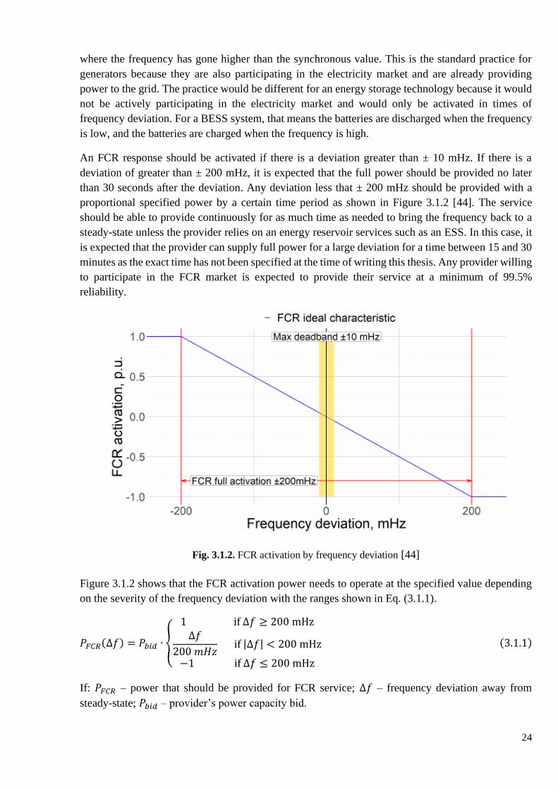
An FCR response should be activated if there is a deviation greater than ± 10 mHz. If there is a

deviation of greater than ± 200 mHz, it is expected that the full power should be provided no later

than 30 seconds after the deviation. Any deviation less that ± 200 mHz should be provided with a

proportional specified power by a certain time period as shown in Figure 3.1.2 [44]. The service

should be able to provide continuously for as much time as needed to bring the frequency back to a

steady-state unless the provider relies on an energy reservoir services such as an ESS. In this case, it

is expected that the provider can supply full power for a large deviation for a time between 15 and 30

minutes as the exact time has not been specified at the time of writing this thesis. Any provider willing

to participate in the FCR market is expected to provide their service at a minimum of 99.5%

reliability.

Fig. 3.1.2. FCR activation by frequency deviation [44]

Figure 3.1.2 shows that the FCR activation power needs to operate at the specified value depending

on the severity of the frequency deviation with the ranges shown in Eq. (3.1.1).

𝑃𝐹𝐶𝑅(∆𝑓) = 𝑃𝑏𝑖𝑑 ∙ {

1 if ∆𝑓 ≥ 200 mHz∆𝑓

200 𝑚𝐻𝑧 if |∆𝑓| < 200 mHz

−1 if ∆𝑓 ≤ 200 mHz

(3.1.1)

If: 𝑃𝐹𝐶𝑅 – power that should be provided for FCR service; ∆𝑓 – frequency deviation away from

steady-state; 𝑃𝑏𝑖𝑑 – provider’s power capacity bid.

25

The procurement of the FCR reserves is expected to be in daily auctions that can be set until a day in

advance. The bids can start at a minimum of 1 MW and increment at a bid resolution of 1 MW. The

bids for a certain day will be for 6 independent products covering a period of 4 hours (0-4h, 4-8h, 8-

12h, 12-16h, 16-20h, 20-24h). The auction will work in a marginal bidding process where each

provider will bid their available capacity and the price at which they are willing to provide that

capacity. The required capacity is then added up from the lowest bids until the required capacity is

met and set to the price of final bid that meets the total threshold.

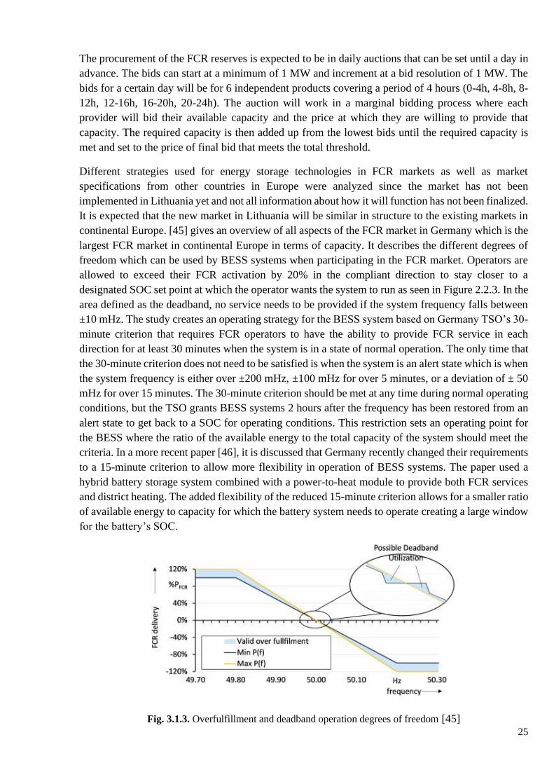
Different strategies used for energy storage technologies in FCR markets as well as market

specifications from other countries in Europe were analyzed since the market has not been

implemented in Lithuania yet and not all information about how it will function has not been finalized.

It is expected that the new market in Lithuania will be similar in structure to the existing markets in

continental Europe. [45] gives an overview of all aspects of the FCR market in Germany which is the

largest FCR market in continental Europe in terms of capacity. It describes the different degrees of

freedom which can be used by BESS systems when participating in the FCR market. Operators are

allowed to exceed their FCR activation by 20% in the compliant direction to stay closer to a

designated SOC set point at which the operator wants the system to run as seen in Figure 2.2.3. In the

area defined as the deadband, no service needs to be provided if the system frequency falls between

±10 mHz. The study creates an operating strategy for the BESS system based on Germany TSO’s 30-

minute criterion that requires FCR operators to have the ability to provide FCR service in each

direction for at least 30 minutes when the system is in a state of normal operation. The only time that

the 30-minute criterion does not need to be satisfied is when the system is an alert state which is when

the system frequency is either over ±200 mHz, ±100 mHz for over 5 minutes, or a deviation of ± 50

mHz for over 15 minutes. The 30-minute criterion should be met at any time during normal operating

conditions, but the TSO grants BESS systems 2 hours after the frequency has been restored from an

alert state to get back to a SOC for operating conditions. This restriction sets an operating point for

the BESS where the ratio of the available energy to the total capacity of the system should meet the

criteria. In a more recent paper [46], it is discussed that Germany recently changed their requirements

to a 15-minute criterion to allow more flexibility in operation of BESS systems. The paper used a

hybrid battery storage system combined with a power-to-heat module to provide both FCR services

and district heating. The added flexibility of the reduced 15-minute criterion allows for a smaller ratio

of available energy to capacity for which the battery system needs to operate creating a large window

for the battery’s SOC.

Fig. 3.1.3. Overfulfillment and deadband operation degrees of freedom [45]

26

Different control strategies were analyzed in [47] for battery usage in West-Denmark’s FCR market

based on different state of charge set points. Their bidding strategy assumed bids were won for all

service times to be able to provide the maximum amount of power. This study found that having a

higher setpoint for the state of charge in the battery system allowed for higher revenues early on, but

increased battery degradation causes the batteries to have a lower a lifetime and a lower NPV.

3.2 Battery Degradation

The battery life and type of battery system that is used needs to be carefully considered due to the

need of the FCR service to either absorb or provide power throughout the day at fast response times.

If too much battery life is lost in the system, it may no longer qualify at its previous volumes and this

would reduce the amount of money that can be made from the FCR service.

The calculation of battery degradation throughout its lifetime is calculated with two important factors

of calendar aging and cycle aging [43, 48, 49]. These two aging factors added together can give an

evaluation of the total capacity lost by a battery. In [43], a lifetime estimation model for LFP batteries

was created and calculations for the calendar and cycle capacity fading were found and tested against

real performance of an LFP system.

𝐶𝑓𝑎𝑑𝑒,𝑐𝑎𝑙 = 3.087 ∙ 10−7 × 𝑒0.05146𝑇 × 𝑡0.5 (3.2.1)

𝐶𝑓𝑎𝑑𝑒,𝑐𝑦𝑐𝑙𝑒 = 6.87 ∙ 10−5 × 𝑒0.027𝑇 × 𝑁𝐶0.5 (3.2.2)

If: 𝐶𝑓𝑎𝑑𝑒,𝑐𝑎𝑙 – percentage of battery capacity lost due to calendar fading; 𝑡 – time in number of months;

𝐶𝑓𝑎𝑑𝑒,𝑐𝑦𝑐𝑙𝑒 – percentage of battery capacity lost due to cycle fading; 𝑇 – temperature in Kelvins; 𝑁𝐶

-number of full cycles done by the battery.

3.3 FCR Model

This model simulates a BESS system that provides FCR services for a span of 16 years and calculates

if the system is viable investments after the time has concluded. The requirements of the FCR market

used for this simulation were based on the data currently available from Lithuania’s future FCR

market as well as information from other existing markets that were covered in the literature review.

The specifications of this model are recorded below in Figure 3.3.1.

Table 3.3.1: FCR specifications

Parameter Value

Minimum bid 1 MW

Divisibility of bids 1 MW

Bid service time 4 hours

Deadband ±10 mHz

Full activation frequency deviation ±200 mHz, ±100mHz if > 5

min, ±50 mHz >15 min

Full activation time 30 seconds

Max supply time for full activation 15 minutes

Minimum Reliability 99.5%

27

3.4 BESS System Specifications

The most important constraint for the operation of the BESS system is the 15-minute criterion. The

battery should have enough capacity to either charge or discharge power in each direction when in a

normal operating state. The SOC should be kept around an operating point that will allow the system

to meet this requirement with the consideration that it needs to supply its full FCR power for 15

minutes in the worst-case scenario. The upper bound of the SOC and the lower bound are limited to

the time and the ratio of the FCR service power and the energy capacity of the BESS system.

𝑆𝑂𝐶𝑈𝐵 = 1 −0.25ℎ𝑟 ∙ 𝑃𝑏𝑖𝑑

𝐶 (3.4.1)

𝑆𝑂𝐶𝐿𝐵 =0.25ℎ𝑟 ∙ 𝑃𝑏𝑖𝑑

𝐶 (3.4.2)

If: 𝑆𝑂𝐶𝑈𝐵 – SOC upper limit; 𝑃𝐹𝐶𝑅 – power capacity bid by provider; 𝐶 – energy capacity of BESS

𝑆𝑂𝐶𝐿𝐵 – SOC lower limit.

The state of charge should fall somewhere between the lower and upper bounds at any point during

normal operation. The flexibility of the SOC range increases as the ratio between the capacity and

the provided power increases as seen in Figure 4.2.1. The area between the two bounds is the

permitted operating SOC of the BESS system. Having a larger capacity compared to the bid power

allows a wider range of operation of the SOC system, but a higher capacity will increase the

investment cost of the BESS system. If the SOC reaches the boundaries of operation, the model will

stop FCR operation and either charge or discharge to get back to an operating state of charge. The

time that the battery is not operating to return to an FCR state is recorded as time not compliant and

goes against its reliability percentage in the simulation. A reliability lower than 99.5% means that the

system would not meet the required condition set by the TSO.

Fig. 3.4.1. Permitted operating SOC range of BESS system

28

The battery capacity degradation is calculated using the Equations 3.2.1 and 3.2.2 discussed

previously. The BESS system is assumed to always operate at a temperature of 25 degrees Celsius.

At the end of each simulation year, the capacity degradation values are updated. Equation 3.2.2 is

based off full cycles of operation which do not occur in FCR operation. The battery usually operates

at smaller depths of discharge due to the changes of the system frequency. The model incorporates a

method to calculate the smaller operating cycles of the BESS. In [50, 51], the rainflow counting

algorithm is used to count the number of cycles at different DOD throughout a battery lifetime. The

Palmgren-Miner rule is then used to calculate the weight of that DOD compared to a full cycle. The

rainflow counting function in MATLAB was used to calculate the different cycles that a battery

performed in each year, but the data was first adjusted to only count cycles of DOD greater than 1%.

This was done to lower operating time by reducing the number of cycles calculated that do not

contribute significantly to the cycle battery degradation. Figure 4.2.2 shows a week of data for battery

SOC and how the data is filtered before calculation in the RFC function. The real data shows that

there are many small adjustments to the SOC throughout a day that will not be counted in RFC

because their DOD is very small. The cycles larger than 1% DOD are calculated throughout the year

and adjusted to a weight comparable to a full cycle.

Fig. 3.4.2. SOC during one day for BESS model and adjusted for RFC

The Palmgren-Miner rule is used to find the adjusted weight of a battery cycle in this simulation

compared to a cycle at the full depth of discharge. The smaller the DOD of the cycle, the more cycles

the battery can endure before its end of life is reached. The ratio used to calculate the weighted factor

is:

29

𝐶𝑦𝑐𝑊𝐹 =𝑁𝐹,𝑐𝑦𝑐

𝑁𝑖,𝑐𝑦𝑐 (3.4.3)

If: 𝐶𝑦𝑐𝑊𝐹 – weighted factor; 𝑁𝐹,𝑐𝑦𝑐 – number of cycles that battery can perform at full DOD before

its end of life; 𝑁𝑖,𝑐𝑦𝑐 – number of cycles the battery can perform at the current DOD.

A battery is needed to model the number of cycles for each depth of discharge and in this simulation

data specifications were used from Saft’s Synerion 48M lithium ion module [52]. The cycle life data

was taken from the specifications to create a best-fit line for the number of cycles the battery can

perform at each DOD before its EOL of 70% capacity.

𝑁𝑖,𝑐𝑦𝑐 = 6 ⋅ 106 × 𝐷𝑂𝐷𝑖−1.168 (3.4.4)

If: 𝑁𝑖,𝑐𝑦𝑐 – number of cycles the battery can perform at the specific DOD; 𝐷𝑂𝐷𝑖 – depth of discharge

percentage.

The battery is expected to function until it reaches 70% of its original capacity when it will reach its

EOL. According to Saft A plot of the manufacturer’s battery DOD testing in Figure 3.4.3 [52] shows

the battery can perform many more cycles of smaller DOD before reaching its EOL. The datasheet

also specifies that the battery’s lifetime is designed to last 20 years. Figure 2.2.4 shows the number

of cycles at different DOD that a BESS of 1MW/2MWh completes in one year of operation. The

majority of the battery’s DOD cycles are between 0-5%.

Fig. 3.4.3. Battery cycles before 70% EOL capacity for DOD of cycle [52]

30

Fig. 3.4.4: Cycles for different DOD in a year for 1MW/2MWh BESS

3.5 Frequency and Market Data

The frequency data used for this model came from RTE in France [53]. RTE has yearly frequency

data-sets that are the most easily accessible of countries in continental Europe with a frequency

control market and they do not require users to have an affiliation with a French organization to access

their frequency data. The data is a time series of frequency measurements at 10-second intervals and

the measurements span for two years from 2019-2020 to get a variety of measurements throughout

different seasons. There were some locations of missing data and the missing values were filled using

linear interpolation if the missing values were less than one minute. If the missing time was greater

than a minute, the measurements were filled with values belonging to the same seasonal period. The

date of January 10, 2019 was also removed from the dataset as the examined data had very large

frequency fluctuations. It was reported by ENTSO-E [54] that continental Europe experienced

uncharacteristic frequency deviations on this day due to frozen measurements on four interconnection

lines. The data did not represent the frequency of a typical day, so the data was removed to leave two

years of data equaling 365 days each. The total missing values for the 2-year period totaled less than

four days. As seen in Figure 3.5.1, the majority of the measurements recorded are closer to the steady

state of 50 Hz and less occurrences are recorded when moving farther away from this value. There

are also slightly more occurrences for frequencies greater than 50 Hz. The probability for the different

measurements of the frequency is plotted in Figure 3.5.2. This gives a better visualization for the

power that should be provided by the FCR service. The highest probability is that the measurement

will be in the deadband, meaning that the service is not required to be provided there. There is a

slightly higher probability that the frequency is greater than 50 Hz and the BESS needs to be

discharged to provide FCR service proportional to the deviation compared to scenarios where the

frequency is less than 50 Hz, and the BESS should charge at a proportional rate. In the two-year span,

there were no occurrences where the frequency deviated greater than 200 mHz and the full FCR

31

service is required to be provided. The longest operating alert states were also checked in the data to

see where the BESS system would be allowed to violate the 15-minute criterion. The longest

deviation of over ± 100 mHz lasted 6 minutes and 40 seconds, and the longest deviation of over ± 50

mHz lasted for 22 minutes and 40 seconds.

Fig. 3.5.1. Grid frequency measurements over 2-year period

Fig. 3.5.2. Probability of Grid Frequency over 2-year period

32

The FCR price data used for this simulation was taken from Germany’s FCR market that is currently

in operation [55]. Since July of 2020, Germany has switched from bids of one-day FCR service, to

six, four-hour blocks of bid service for their FCR market. This is the same structure that is expected

for Lithuania’s FCR market. The price data was taken from Germany instead of France because the

dataset lists the prices at 4-hour increments while data from France is in 30-minute increments. The

data collected is only representative of 274 days because the new structure has not yet been in

operation for a full year. The remaining 91 days were filled by randomly selecting a date from the

data set to complete a full year of prices. A histogram of the probabilities of the different prices is

shown in Figure 4.3.3. The majority of the FCR prices throughout the year are between €20-40/MW

for FCR service provided in a 4-hour period. The total price for service provided for every block in a

year sums to €64,326/MW of FCR service provided. In this simulation, it is assumed that the FCR

provider would bid for every block of service because the batteries are readily available and do not

need a ramp-up time like spinning reserves.

Fig. 3.5.3. Probability of FCR prices for one year

In scenarios where the BESS is reaching the upper or lower SOC limit, the battery will need to charge

or discharge back to an equilibrium SOC before resuming operation to satisfy the 15-minute criterion.

The BESS system will use the intraday market to either buy or sell power to return to operating levels.

The FCR service will be stopped for 30 minutes while the BESS exchanges power in the intra-day

electricity market. This model is focused on analyzing the BESS’s participation as an FCR provider

and not as a provider in the intraday market. Therefore, the model uses a value of €35/MWh for

buying and selling electricity throughout the whole simulation. The power that is exchanged is

calculated at increments of 0.1 MW.

33

3.6 Costs Calculation

The model uses net present value to calculate whether the project is a worthy investment. NPV can

be calculated as:

𝑁𝑃𝑉 = ∑𝐶𝐹

(1 + 𝑟)𝑡

𝑇

𝑡=0

(3.6.1)

If: 𝑁𝑃𝑉 – net present value; 𝐶𝐹 – cash flow; 𝑟 – discount rate; 𝑡 – current year of the calculation; 𝑇

– total years of the calculation.

An investment is worth pursuing if at the end of the calculation, the NPV is either zero or a positive

value. The discount rate is a percentage associated with inflation and the risk of a project. The cash

flow is a difference between the revenue made for that year minus the costs spent that year on the

project related to investment and maintenance. The cash flow in this model was calculated with the

following factors:

𝐶𝐹 = 𝐹𝐶𝑅 + 𝐼𝐷𝑆𝑒𝑙𝑙 − 𝐼𝑛𝑣𝑒𝑠𝑡𝑚𝑒𝑛𝑡 − 𝑂𝑀 − 𝐼𝐷𝑏𝑢𝑦 (3.6.2)

If 𝐶𝐹 – cash flow; 𝐹𝐶𝑅 – money earned from providing FCR service in a year; 𝐼𝐷𝑆𝑒𝑙𝑙 – money earned

from selling power on the intraday market in that year; 𝐼𝑛𝑣𝑒𝑠𝑡𝑚𝑒𝑛𝑡 – cost of investment from the

battery system; 𝑂&𝑀 is the yearly operation and maintenance cost of the BESS system; 𝐼𝐷𝑏𝑢𝑦 – the

money spent buying electricity on the intraday market.

The cash flow will change every year as the battery degrades lowering the energy capacity. The

different costs used to calculate the FCR model can be seen in Table 3.6.1.

Table 3.6.1. Costs for model simulation calculation

Parameter Cost

FCR per year €64,326/MW

Intraday buy/sell €35/MWh

BESS investment €600/kWh

Misc. Investment (inverter,

transformer, etc.)

€100/kW

Operation and maintenance cost

per year

€6/kW

Discount rate 5%

3.7 Algorithm of Model

The model in the system records the SOC at every time step in a year to calculate how the BESS

should behave and count the cycles occurring at different DODs. The data is at 10-second time

intervals and there are 360-time intervals within an hour. The SOC is a number between 1-100 that

represents the percentage of charge available in the BESS. The SOC of the BESS at each time is

dependent on the SOC from the previous time where the BESS is operating. Section 3.1 shows that

during a steady state for the system frequency, the SOC will remain the same from the previous time.

34

If there is a deviation less than 49.99 Hz, the BESS will discharge at a rate proportional to the to the

frequency deviation and the SOC of the next time step can be found with:

𝑆𝑂𝐶(𝑡 + 1) = 𝑆𝑂𝐶(𝑡) − (𝑃𝐹𝐶𝑅(∆𝑓)

360×

100

𝐶𝑎𝑝×

1

𝜂𝑏𝑎𝑡𝑡 ∙ 𝜂𝑖𝑛𝑣 ∙ 𝜂𝑡𝑟𝑎𝑛) (3.7.1)

If: 𝑆𝑂𝐶(𝑡 + 1) – SOC of next time step; 𝑆𝑂𝐶(𝑡) – current SOC of the BESS, 𝑃𝐹𝐶𝑅(∆𝑓) – proportional

FCR power provided dependent on the frequency deviation; 𝐶𝑎𝑝 – energy capacity of the BESS;

𝜂𝑏𝑎𝑡𝑡 – discharging efficiency of the BESS; 𝜂𝑖𝑛𝑣 – inverter efficiency; 𝜂𝑡𝑟𝑎𝑛 – transmission efficiency.

The efficiencies used in this model are shown in Table 4.5.1. In a scenario where the frequency of

the system greater than 50.01 Hz, the SOC at the next time step can be found with a similar

calculation:

𝑆𝑂𝐶(𝑡 + 1) = 𝑆𝑂𝐶(𝑡) + (𝑃𝐹𝐶𝑅(∆𝑓)

360×

100

𝐶𝑎𝑝× 𝜂𝑏𝑎𝑡𝑡 ∙ 𝜂𝑖𝑛𝑣 ∙ 𝜂𝑡𝑟𝑎𝑛) (3.7.2)

𝜂𝑏𝑎𝑡𝑡 in this equation is the charging efficiency of the battery and in this model it is the same as the

discharge efficiency. When the battery reaches the upper or lower bound, the battery needs to be

charged or discharged for 30 minutes using the intraday market to return to an operating level. The

calculations of SOC for discharging and charging in intraday market time scenarios is shown in

Equations 4.5.3 and 4.5.4 respectively.

𝑆𝑂𝐶(𝑡 + 1) = 𝑆𝑂𝐶(𝑡) − ((𝑆𝑂𝐶𝑈𝐵 − 0.4) ×𝑃𝑏𝑖𝑑

180×

100

𝐶𝑎𝑝×

1

𝜂𝑏𝑎𝑡𝑡 ∙ 𝜂𝑖𝑛𝑣 ∙ 𝜂𝑡𝑟𝑎𝑛) (3.7.3)

𝑆𝑂𝐶(𝑡 + 1) = 𝑆𝑂𝐶(𝑡) + ((0.6 − 𝑆𝑂𝐶𝐿𝐵) ×𝑃𝑏𝑖𝑑

180×

100

𝐶𝑎𝑝× 𝜂𝑏𝑎𝑡𝑡 ∙ 𝜂𝑖𝑛𝑣 ∙ 𝜂𝑡𝑟𝑎𝑛) (3.7.4)

If: 𝑆𝑂𝐶𝑈𝐵 – upper bound of the BESS; 𝑆𝑂𝐶𝐿𝐵 – lower bound of the BESS; 𝑃𝑏𝑖𝑑 – power that is bid

to provide FCR service.

The SOC is set to a value of 60% when charged and 40% when discharged because deviations usually

happen in the same direction during a time period of a few hours, and it gives the BESS more

flexibility if it needs to continue in the same trend before it reached its bound.

Table 3.7.1: Efficiencies for SOC calculation

Parameter Efficiency

𝜂𝑏𝑎𝑡𝑡 96%

𝜂𝑖𝑛𝑣 97%

𝜂𝑡𝑟𝑎𝑛 98.5%

The algorithm used in this model to calculate the SOC at each time step of the FCR service is shown

in Figure 4.5.1. The model is dependent on the previous state of charge and the current measurement

of the system frequency. The system frequency data spans two years and is iterated through 8 times

for 16 years of simulation.

35

Fig. 3.7.1: Algorithm to calculate SOC

The program starts by checking if the system is currently in the process of completing an intraday

market transaction. These transactions last 30 minutes in this simulation to get the BESS system back

to an operating state so that it can resume providing FCR service. The program then checks if the

BESS system has reached either its upper or lower boundary of SOC for operation. If it has reached

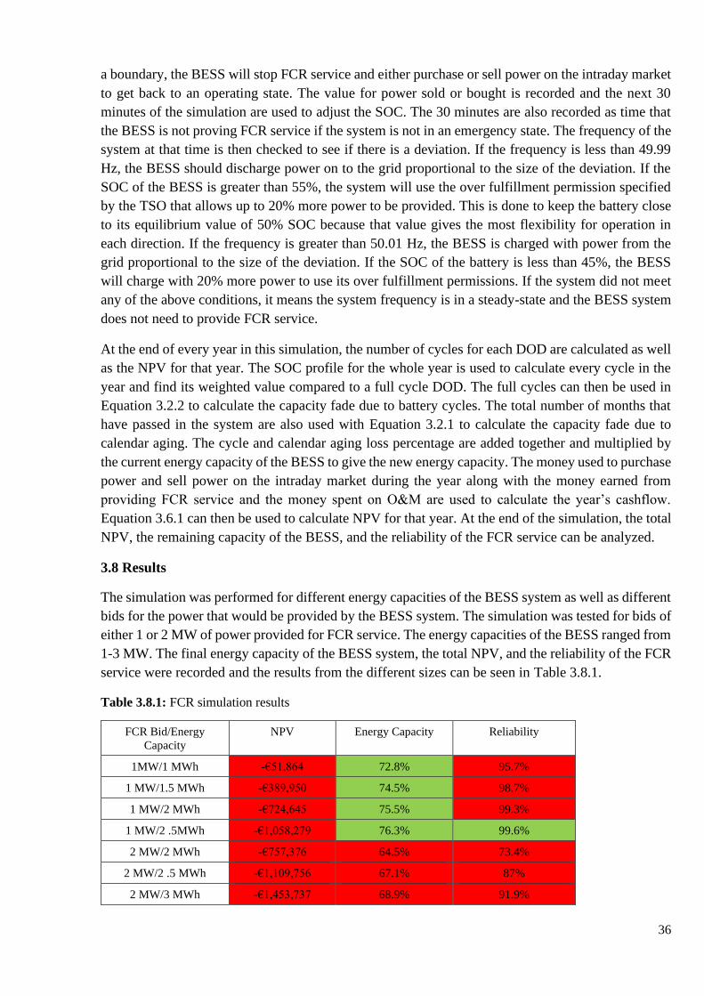
36

a boundary, the BESS will stop FCR service and either purchase or sell power on the intraday market

to get back to an operating state. The value for power sold or bought is recorded and the next 30

minutes of the simulation are used to adjust the SOC. The 30 minutes are also recorded as time that

the BESS is not proving FCR service if the system is not in an emergency state. The frequency of the

system at that time is then checked to see if there is a deviation. If the frequency is less than 49.99

Hz, the BESS should discharge power on to the grid proportional to the size of the deviation. If the

SOC of the BESS is greater than 55%, the system will use the over fulfillment permission specified

by the TSO that allows up to 20% more power to be provided. This is done to keep the battery close

to its equilibrium value of 50% SOC because that value gives the most flexibility for operation in

each direction. If the frequency is greater than 50.01 Hz, the BESS is charged with power from the

grid proportional to the size of the deviation. If the SOC of the battery is less than 45%, the BESS

will charge with 20% more power to use its over fulfillment permissions. If the system did not meet

any of the above conditions, it means the system frequency is in a steady-state and the BESS system

does not need to provide FCR service.

At the end of every year in this simulation, the number of cycles for each DOD are calculated as well

as the NPV for that year. The SOC profile for the whole year is used to calculate every cycle in the

year and find its weighted value compared to a full cycle DOD. The full cycles can then be used in

Equation 3.2.2 to calculate the capacity fade due to battery cycles. The total number of months that

have passed in the system are also used with Equation 3.2.1 to calculate the capacity fade due to

calendar aging. The cycle and calendar aging loss percentage are added together and multiplied by

the current energy capacity of the BESS to give the new energy capacity. The money used to purchase

power and sell power on the intraday market during the year along with the money earned from

providing FCR service and the money spent on O&M are used to calculate the year’s cashflow.

Equation 3.6.1 can then be used to calculate NPV for that year. At the end of the simulation, the total

NPV, the remaining capacity of the BESS, and the reliability of the FCR service can be analyzed.

3.8 Results

The simulation was performed for different energy capacities of the BESS system as well as different

bids for the power that would be provided by the BESS system. The simulation was tested for bids of

either 1 or 2 MW of power provided for FCR service. The energy capacities of the BESS ranged from

1-3 MW. The final energy capacity of the BESS system, the total NPV, and the reliability of the FCR

service were recorded and the results from the different sizes can be seen in Table 3.8.1.

Table 3.8.1: FCR simulation results

FCR Bid/Energy

Capacity

NPV Energy Capacity Reliability

1MW/1 MWh -€51,864 72.8% 95.7%

1 MW/1.5 MWh -€389,950 74.5% 98.7%

1 MW/2 MWh -€724,645 75.5% 99.3%

1 MW/2 .5MWh -€1,058,279 76.3% 99.6%

2 MW/2 MWh -€757,376 64.5% 73.4%

2 MW/2 .5 MWh -€1,109,756 67.1% 87%

2 MW/3 MWh -€1,453,737 68.9% 91.9%

37

The results show that none of the sizes are a financially viable investment to provide FCR service

given the current prices to invest in BESS and the revenues brought in from providing FCR service.

Increasing the power bid from 1 MW to 2 MW causes the BESS system to provide twice the power

and causes the BESS to go through more cycles. During the simulation it reached the threshold more

times needed to trade power on the intraday market and this lowered its reliability score. The process

of going through more cycles also caused a higher capacity degradation due to cycle losses. The

simulations tested at the higher bid power all had a final energy capacity of less then 70% which

means the battery would have already reached its end of life before the 16-year simulation was over.

The starting energy capacity of the BESS system would need to be a higher value to increase the

reliability score and ensure the battery does not reach its end of life before the end of the simulation,

but this would require more initial investment and the NPV for these scenarios is already poor.

The most promising scenarios for the BESS were to provide 1 MW of FCR service and to have an

initial energy capacity of 2 MWh or 2.5 MWh. The 2.5 MWh system had a reliability within the

specifications provided by the TSO while the 2 MWh system was close to achieving the threshold.

Both systems did not reach their EOL by the time the simulation ended but neither system was able

to finish with a NPV that is either positive or 0 before the end of the 16-year simulation. The cost that

the initial investment for the BESS system would need to have to reach a 0 NPV while all other cost

variables stayed the same was checked along with the price for a year’s worth of FCR service to reach

a 0 NPV while other variables stayed the same.

Table 3.8.2. Analysis of hypothetical prices to achieve 0 NPV

BESS Price of BESS investment Price FCR service for a year

1 MW/ 2 MWh €237/kWh €132,000/MW

1 MW/ 2.5 MWh €176/kWh €162,000/MW

The price of investment in the BESS would need to fall between €176-237/kWh to have a 2-2.5 MWh

BESS system that would be a worthy investment if all other prices within the simulation stayed the

same. In [4], it is believed that the price of LFP batteries can drop below €250 kWh after the year

2030. Although battery prices are not an adequate price currently, FCR service with BESS could be

possible in the future. It is also unclear at what prices the FCR service bids will be set once the new

market opens. In [56], it can be seen that historic prices of the German FCR market were higher 5

years ago with yearly revenues of service reaching the €132,000 threshold to make the 1 MW/ 2 MWh

BESS profitable. The prices for the service have decreased as the years have progressed and this

model was performed at a much lower €64,326/MW for FCR service provided. The increase in

providers participating in the German FCR market has caused the prices to decrease through the years.

It is possible that the same scenario could happen in Lithuania with less participants in the first year

of the FCR market and decreasing prices as more participants enter in the future.

3.9 FCR Conclusion

A frequency containment reserve market in Lithuania will be created in the future and an analysis

on the economic viability of providing the service with a BESS was analyzed. A simulation was

created that used frequency time series data to check how a battery would behave at different time

periods of operation. The SOC of the BESS system was checked throughout the 16-year simulation

to check how many cycles it had performed, and this information was used to calculate the capacity

38

degradation experienced by the BESS every year. At the end of the simulation, the system was

checked to see the NPV of the investment, the energy capacity of the BESS, and the reliability of

providing the FCR service. Providing 1 MW of FCR service and having a BESS with an energy

capacity size between 2-2.5 MW provides a system that most closely meets the requirements to

provide FCR service. Although, none of the systems analyzed were deemed a good investment

based on their NPV value at the end of the simulation.

The current cost of investment for lithium-ion batteries is too high to be a viable investment in

providing FCR services. The average cost would need to drop from todays €600 kWh to a much

lower price of around €240-170 kWh. Some research has shown that the cost of LFP batteries can

drop to below €250 kWh after the year 2030. There is a possibility that this could become a viable

investment in the future. There is currently no data for the bid prices on the FCR market in

Lithuania because it has not been implemented yet. The data used in this simulation came from

Germany’s FCR market. It is unknown if the price will be higher or lower than what was used in

this simulation or how the prices will change as the years progress. Data has shown that as years

have progressed in European FCR markets, the prices have been decreasing as more providers join

the market lowering the price. Too many providers in Lithuania’s FCR market could cause the

revenues made from FCR service to decrease and make it more difficult for the BESS to profit.

39

Conclusion

This thesis analyzed two different methods of how energy storage can be used in the grid, with one

method at the distribution level for energy reserve in a microgrid and another method at the

transmission level to provide FCR service. The conclusions of the simulations of the two methods are

described below.

1. The optimal sizing for the microgrid included no battery storage capacity in the final

solution. The current cost of batteries is too high to justify their use in a grid connected

microgrid to provide energy reserves. The cost of purchasing power from the main grid is

much lower than the investment cost associated with a BESS storage installation.

2. The microgrid simulation only accounted for a grid-connected microgrid and not for a

microgrid that can switch to an “islanded mode” or that is completely disconnected from the

grid. The cost of these methods will be higher because they will require more DG and storage

to be independent from the main grid. The consumer’s decision on whether it is a viable

investment for these scenarios would depend on how critically they value their load and the

opportunity cost from a loss of power.

3. The optimal solution showed that installing 1,413 PV panels would create a savings of €

474,061 compared to a consumer who only purchases power from the main grid over a 12-

year period. This solution shows that the cost of PV today is competitive with the costs of

purchasing power from the main grid. If there was a large increase of PV installation by

consumers, this would cause a problem, as reduced power capacity would be produced by

centralized generation stations. This would then require energy storage which this simulation

shows is not currently at an adequate cost. An increase in DG from RES will require

governments to assist in subsidies to offset energy storage costs to move away from large

carbon emitting generation stations.

4. The FCR simulation found that none of the battery sizing systems were deemed a profitable

investment at the end of the 16-year simulation. The 1 MW/2.5 MW was the only tested

system that had not reached its EOL and met the minimum reliability requirements at the

end of the simulation while the 1 MW/2 MW system was close to achieving the reliability

threshold.

5. An increase in the FCR service bid size from 1 MW to 2 MW will require more energy

capacity for the BESS system and that will make it more expensive and reduce the NPV of

the investment. More money can be made by the higher bid, but a smaller energy capacity

causes the BESS to reach its thresholds more often and it must use the real-time market to

adjust its SOC many more times. This also lowers the reliability of the system a lot more

and moves it farther away from the reliability threshold. The smaller capacity also aggregates

many more full cycles into the battery’s life increasing the cycle degradation. The BESS

sizes that were simulated with a 2 MW bid reached their EOL before the 16-year simulation

was over. Lowering the minimum bid requirement to values less that 1 MW and allowing

incrementing bids at a lower step than 1 MW would give providers more flexibility on the

system constraints to meet the necessary thresholds.

40

6. Although the system was not profitable with present day costs, the projected lithium-ion

battery costs after 2030 could make this project profitable at a future date. Higher frequency

containment reserve market prices as they were in the past in other European countries could

also make the project profitable, but historically these markets have seen lower prices each

year as more participants have entered the market. A provider that may enter the market

should consider that the revenues could drop as more providers enter the market throughout

the years.

41

References

1. UECKERDT, Falko, BRECHA, Robert and LUDERER, Gunnar. Analyzing Major

Challenges of Wind and Solar Variability in Power Systems. . P. 21.

2. CHALAMALA, Dr Babu. Grid Energy Storage Technologies and the Future Electric Grid.

Sandia National Labratories.

3. KIPTOO, Mark Kipngetich, LOTFY, Mohammed Elsayed, ADEWUYI, Oludamilare Bode,

CONTEH, Abdul, HOWLADER, Abdul Motin and SENJYU, Tomonobu. Integrated

approach for optimal techno-economic planning for high renewable energy-based isolated

microgrid considering cost of energy storage and demand response strategies. Energy

Conversion and Management. 1 July 2020. Vol. 215, p. 112917.

DOI 10.1016/j.enconman.2020.112917.

4. ELECTRICITY STORAGE AND RENEWABLES: COSTS AND MARKETS TO 2030.

[online]. [Accessed 6 January 2021]. Available from: https://www.irena.org/-

/media/Files/IRENA/Agency/Publication/2017/Oct/IRENA_Electricity_Storage_Costs_201

7.pdf

5. ANEKE, Mathew and WANG, Meihong. Energy storage technologies and real life

applications – A state of the art review. Applied Energy. 1 October 2016. Vol. 179, p. 350–

377. DOI 10.1016/j.apenergy.2016.06.097.

6. PEÑA-ALZOLA, R., SEBASTIÁN, R., QUESADA, J. and COLMENAR, A. Review of

flywheel based energy storage systems. In : 2011 International Conference on Power

Engineering, Energy and Electrical Drives. May 2011. p. 1–6.

7. KHAMIS, A., BADARUDIN, Z. M., AHMAD, A., RAHMAN, A. A. and HAIRI, M. H.

Overview of mini scale Compressed Air Energy Storage System. In : 2010 4th International

Power Engineering and Optimization Conference (PEOCO). June 2010. p. 458–462.

8. HE, Wei, LUO, Xing, EVANS, David, BUSBY, Jonathan, GARVEY, Seamus, PARKES,

Daniel and WANG, Jihong. Exergy storage of compressed air in cavern and cavern volume

estimation of the large-scale compressed air energy storage system. Applied Energy. 15

December 2017. Vol. 208, p. 745–757. DOI 10.1016/j.apenergy.2017.09.074.

9. LEUNG, Puiki, LI, Xiaohong, LEÓN, Carlos Ponce de, BERLOUIS, Leonard, LOW, C. T.

John and WALSH, Frank C. Progress in redox flow batteries, remaining challenges and their

applications in energy storage. RSC Advances. 8 October 2012. Vol. 2, no. 27, p. 10125–

10156. DOI 10.1039/C2RA21342G.

10. KYRIAKOPOULOS, Grigorios L. and ARABATZIS, Garyfallos. Electrical energy storage

systems in electricity generation: Energy policies, innovative technologies, and regulatory

regimes. Renewable and Sustainable Energy Reviews. 1 April 2016. Vol. 56, p. 1044–1067.

DOI 10.1016/j.rser.2015.12.046.

11. TEAM, E. F. Y. Electronics With Lithium-Ion Batteries | Must Read. Electronics For You

[online]. 13 August 2020. [Accessed 10 May 2021]. Available from:

https://www.electronicsforu.com/market-verticals/power-electronics/lithium-ion-batteries

12. THORBERGSSON, E., KNAP, V., SWIERCZYNSKI, M., STROE, D. and

TEODORESCU, R. Primary Frequency Regulation with Li-Ion Battery Based Energy

Storage System - Evaluation and Comparison of Different Control Strategies. In : Intelec

42

2013; 35th International Telecommunications Energy Conference, SMART POWER AND

EFFICIENCY. October 2013. p. 1–6.

13. NADEEM, F., HUSSAIN, S. M. S., TIWARI, P. K., GOSWAMI, A. K. and USTUN, T. S.

Comparative Review of Energy Storage Systems, Their Roles, and Impacts on Future Power

Systems. IEEE Access. 2019. Vol. 7, p. 4555–4585. DOI 10.1109/ACCESS.2018.2888497.

14. Battery Storage in the United States: An Update on Market Trends. U.S. Energy

Information Administration.

15. PJM Manual 12: Balancing Operations. 27 January 2021. PJM.

16. COMMISSION, California Energy. Energy Storage Targets - Publicly Owned Utilities - AB

2514. California Energy Commission [online]. current-date. [Accessed 13 May 2021].

Available from: https://www.energy.ca.gov/data-reports/reports/energy-storage-targets-

publicly-owned-utilities

17. Decision on Participation of Non-Generator Resources in ISO Ancillary Services Markets.

17 March 2010. CAISO.

18. THE VALUE OF ELECTRICITY STORAGE An outlook on services and market

opportunities in the Danish and international electricity markets. 6 February 2020. Ea

Energy Analyses.

19. AutoGrid Deploys AutoGrid Flex for Total’s Largest Battery-Based Energy Storage Project

in France. [online]. 23 February 2021. [Accessed 13 May 2021]. Available from:

https://www.businesswire.com/news/home/20210223005339/en/AutoGrid-Deploys-

AutoGrid-Flex-for-Total%E2%80%99s-Largest-Battery-Based-Energy-Storage-Project-in-

FranceAutoGrid, the market leader in AI-powered flexibility management software for the

energy industry, deploys award-winning AutoGrid FlexTM Virtual Power

20. France’s biggest battery storage system at 25MW goes into operation. Energy Storage News

[online]. [Accessed 20 May 2021]. Available from: https://www.energy-

storage.news/news/frances-biggest-battery-storage-system-at-25mw-goes-into-operationThe

biggest battery energy storage system (BESS) in mainland France went into operation in late

January, and will provide grid-balancing services to national transmission system operator

RTE.

21. YOU, Shi, HU, Junjie and ZIRAS, Charalampos. An Overview of Modeling Approaches

Applied to Aggregation-Based Fleet Management and Integration of Plug-in Electric

Vehicles †. Energies. November 2016. Vol. 9, no. 11, p. 968. DOI 10.3390/en9110968.

22. TOMIĆ, Jasna and KEMPTON, Willett. Using fleets of electric-drive vehicles for grid

support. Journal of Power Sources. 1 June 2007. Vol. 168, no. 2, p. 459–468.

DOI 10.1016/j.jpowsour.2007.03.010.

23. SARABI, Siyamak, DAVIGNY, Arnaud, COURTECUISSE, Vincent, RIFFONNEAU,

Yann and ROBYNS, Benoît. Potential of vehicle-to-grid ancillary services considering the

uncertainties in plug-in electric vehicle availability and service/localization limitations in

distribution grids. Applied Energy. 1 June 2016. Vol. 171, p. 523–540.

DOI 10.1016/j.apenergy.2016.03.064.

43

24. PARHIZI, S., LOTFI, H., KHODAEI, A. and BAHRAMIRAD, S. State of the Art in

Research on Microgrids: A Review. IEEE Access. 2015. Vol. 3, p. 890–925.

DOI 10.1109/ACCESS.2015.2443119.

25. STADLER, Michael and NASLÉ, Adib. Planning and implementation of bankable

microgrids. The Electricity Journal. 1 June 2019. Vol. 32, no. 5, p. 24–29.

DOI 10.1016/j.tej.2019.05.004.

26. MUMTAZ, Faisal and BAYRAM, Islam Safak. Planning, Operation, and Protection of

Microgrids: An Overview. Energy Procedia. 1 February 2017. Vol. 107, p. 94–100.

DOI 10.1016/j.egypro.2016.12.137.

27. FERRARO, Pietro, CRISOSTOMI, Emanuele and MILANO, Federico. Evaluation of the

Impact of the Size of Storage Devices in Grid-Connected Microgrids. In : 2018 IEEE

International Conference on Environment and Electrical Engineering and 2018 IEEE

Industrial and Commercial Power Systems Europe (EEEIC / I CPS Europe). June 2018.

p. 1–5.

28. CAGNANO, A., DE TUGLIE, E. and MANCARELLA, P. Microgrids: Overview and

guidelines for practical implementations and operation. Applied Energy. 15 January 2020.

Vol. 258, p. 114039. DOI 10.1016/j.apenergy.2019.114039.

29. Lithuania electricity prices, June 2020. GlobalPetrolPrices.com [online].

[Accessed 16 January 2021]. Available from:

https://www.globalpetrolprices.com/Lithuania/electricity_prices/

30. KHARRICH, M., SAYOUTI, Y. and AKHERRAZ, M. Optimal microgrid sizing and daily

capacity stored analysis in summer and winter season. In : 2018 4th International

Conference on Optimization and Applications (ICOA). April 2018. p. 1–6.

31. AN, L. N., QUOC-TUAN, T., SEDDIK, B. and VAN-LINH, N. Optimal sizing of a grid-

connected microgrid. In : 2015 IEEE International Conference on Industrial Technology

(ICIT). March 2015. p. 2869–2874.

32. Renewables.ninja. [online]. [Accessed 13 January 2021]. Available from:

https://www.renewables.ninja/

33. PFENNINGER, Stefan and STAFFELL, Iain. Long-term patterns of European PV output

using 30 years of validated hourly reanalysis and satellite data. Energy. 1 November 2016.

Vol. 114, p. 1251–1265. DOI 10.1016/j.energy.2016.08.060.

34. Eu PV report. [online]. [Accessed 30 November 2020]. Available from:

https://ec.europa.eu/jrc/sites/jrcsh/files/kjna29938enn_1.pdf

35. DHUNDHARA, Sandeep, VERMA, Yajvender Pal and WILLIAMS, Arthur. Techno-

economic analysis of the lithium-ion and lead-acid battery in microgrid systems. Energy

Conversion and Management. 1 December 2018. Vol. 177, p. 122–142.

DOI 10.1016/j.enconman.2018.09.030.

36. Energy Storage Technology and Cost Characterization Report. [online].

[Accessed 6 January 2021]. Available from:

https://www.energy.gov/sites/prod/files/2019/07/f65/Storage%20Cost%20and%20Performa

nce%20Characterization%20Report_Final.pdf

44

37. Charging Lithium-Ion Batteries. [online]. [Accessed 15 May 2021]. Available from:

https://batteryuniversity.com/learn/article/charging_lithium_ion_batteriesReview simple

guidelines for charging Lithium-based batteries and prolong battery life such as; a portable

device should be turned off while charging and more.

38. CAO, B., DONG, W., LV, Z., GU, Y., SINGH, S. and KUMAR, P. Hybrid Microgrid

Many-Objective Sizing Optimization With Fuzzy Decision. IEEE Transactions on Fuzzy

Systems. November 2020. Vol. 28, no. 11, p. 2702–2710.

DOI 10.1109/TFUZZ.2020.3026140.

39. HERNÁNDEZ, J. C., MEDINA, A. and JURADO, F. Optimal allocation and sizing for

profitability and voltage enhancement of PV systems on feeders. Renewable Energy. 1

August 2007. Vol. 32, no. 10, p. 1768–1789. DOI 10.1016/j.renene.2006.11.003.

40. KORNELAKIS, Aris and MARINAKIS, Yannis. Contribution for optimal sizing of grid-

connected PV-systems using PSO. Renewable Energy. 1 June 2010. Vol. 35, no. 6, p. 1333–

1341. DOI 10.1016/j.renene.2009.10.014.

41. DALI, A., ABDELMALEK, S., NEKKACHE, A. and BOUHARCHOUCHE, A.

Development of a Sizing Interface for Photovoltaic-Wind Microgrid Based on PSO-LPSP

Optimization Strategy. In : 2018 International Conference on Wind Energy and

Applications in Algeria (ICWEAA). November 2018. p. 1–5.

42. CLARK, Terry. Search Algorithm Series: PSO. Medium [online]. 20 December 2017.

[Accessed 20 May 2021]. Available from: https://medium.com/@iamterryclark/swarm-

intelli-eb5e46eda0c3Particle Swarm Optimisation

43. STROE, D., ŚWIERCZYŃSKI, M., STAN, A., TEODORESCU, R. and ANDREASEN, S.

J. Accelerated Lifetime Testing Methodology for Lifetime Estimation of Lithium-Ion

Batteries Used in Augmented Wind Power Plants. IEEE Transactions on Industry

Applications. November 2014. Vol. 50, no. 6, p. 4006–4017.

DOI 10.1109/TIA.2014.2321028.

44. Baltic Load-Frequency Control block concept document [online]. September 2020. Litgrid.

[Accessed 18 January 2021]. Available from:

https://www.litgrid.eu/uploads/files/dir555/dir27/dir1/17_0.php

45. THIEN, Tjark, SCHWEER, Daniel, STEIN, Denis vom, MOSER, Albert and SAUER, Dirk

Uwe. Real-world operating strategy and sensitivity analysis of frequency containment

reserve provision with battery energy storage systems in the german market. Journal of

Energy Storage. 1 October 2017. Vol. 13, p. 143–163. DOI 10.1016/j.est.2017.06.012.

46. SCHLACHTER, Uli, WORSCHECH, Alena, DIEKMANN, Theys, HANKE, Benedikt and

VON MAYDELL, Karsten. Optimised capacity and operating strategy for providing

frequency containment reserve with batteries and power-to-heat. Journal of Energy Storage.

1 December 2020. Vol. 32, p. 101964. DOI 10.1016/j.est.2020.101964.

47. THORBERGSSON, E., KNAP, V., SWIERCZYNSKI, M., STROE, D. and

TEODORESCU, R. Primary Frequency Regulation with Li-Ion Battery Based Energy

Storage System - Evaluation and Comparison of Different Control Strategies. In : Intelec

2013; 35th International Telecommunications Energy Conference, SMART POWER AND

EFFICIENCY. October 2013. p. 1–6.

45

48. LIU, Kailong, ASHWIN, T. R., HU, Xiaosong, LUCU, Mattin and WIDANAGE, W.

Dhammika. An evaluation study of different modelling techniques for calendar ageing

prediction of lithium-ion batteries. Renewable and Sustainable Energy Reviews. 1 October

2020. Vol. 131, p. 110017. DOI 10.1016/j.rser.2020.110017.

49. FLEER, Johannes, ZURMÜHLEN, Sebastian, BADEDA, Julia, STENZEL, Peter, HAKE,

Jürgen-Friedrich and SAUER, Dirk Uwe. Model-based Economic Assessment of Stationary

Battery Systems Providing Primary Control Reserve. Energy Procedia. 1 November 2016.

Vol. 99, p. 11–24. DOI 10.1016/j.egypro.2016.10.093.

50. BELTRAN, Hector, TOMÁS GARCÍA, Iván, ALFONSO-GIL, José Carlos and PÉREZ,

Emilio. Levelized Cost of Storage for Li-Ion Batteries Used in PV Power Plants for Ramp-

Rate Control. IEEE Transactions on Energy Conversion. March 2019. Vol. 34, no. 1,

p. 554–561. DOI 10.1109/TEC.2019.2891851.

51. AYUSO, Pablo, BELTRAN, Hector, SEGARRA-TAMARIT, Jorge and PÉREZ, Emilio.

Optimized profitability of LFP and NMC Li-ion batteries in residential PV applications.

Mathematics and Computers in Simulation. 1 May 2021. Vol. 183, p. 97–115.

DOI 10.1016/j.matcom.2020.02.011.

52. Synerion 48M [online]. Saft. Available from:

http://www.aegtranzcom.com/Repository/PDF-

ENERGY/Saft_Com_Synerion48M_en_0512_Protg.pdf

53. Download data published by RTE - RTE Services Portal. Portail Services RTE [online].

[Accessed 11 April 2021]. Available from: https://www.services-rte.com/en/download-data-

published-by-rte.html

54. ENSTO-E. [Press Release] ENTSO-E technical report on the January 2019 significant

frequency deviations in Continental Europe. [online]. [Accessed 26 April 2021]. Available

from: https://www.entsoe.eu/news/2019/05/28/entso-e-technical-report-on-the-january-

2019-significant-frequency-deviations-in-continental-europe/

55. Datacenter FCR/aFRR/mFRR. [online]. [Accessed 19 April 2021]. Available from:

https://www.regelleistung.net/apps/datacenter/tendering-

files/?productTypes=FCR&markets=CAPACITY,ENERGY&fileTypes=RESULTS&dateR

ange=2020-01,2021-04

56. BADEDA, Julia, MEYER, Jonas and SAUER, Dirk Uwe. Modeling the influence of

installed battery energy storage systems on the German frequency containment reserve

market. In : NEIS 2017; Conference on Sustainable Energy Supply and Energy Storage

Systems. September 2017. p. 1–7.