General rights Copyright and moral rights for the publications made accessible in the public portal are retained by the authors and/or other copyright owners and it is a condition of accessing publications that users recognise and abide by the legal requirements associated with these rights.

• Users may download and print one copy of any publication from the public portal for the purpose of private study or research. • You may not further distribute the material or use it for any profit-making activity or commercial gain • You may freely distribute the URL identifying the publication in the public portal

If you believe that this document breaches copyright please contact us providing details, and we will remove access to the work immediately and investigate your claim.

Downloaded from orbit.dtu.dk on: Jun 11, 2018

Analysis of carbides and inclusions in high speed tool steels

Therkildsen, Kasper Tipsmark; Dahl, K.V.

Publication date:2002

Document VersionPublisher's PDF, also known as Version of record

Link back to DTU Orbit

Citation (APA):Therkildsen, K. T., & Dahl, K. V. (2002). Analysis of carbides and inclusions in high speed tool steels.(Denmark. Forskningscenter Risoe. Risoe-R; No. 1360(EN)).

Risø-R-1360(EN)

Analysis of carbides and inclusions in high speed tool steels Kasper Tipsmark Therkildsen and Christian Vinter Dahl

Risø National Laboratory, Roskilde August 2002

Abstract The fracture surfaces of fatigued specimens were investigated using scanning electron microscopy (SEM) and energy dispersive x-ray spectroscopy (EDS). The aim was to quantify the distribution of cracked carbides and non-metallic inclusions on the fracture surfaces as well as on polished cross sections. The specimens were made of Böhler P/M steel grade 390s and 690s in both micro-clean and conventional grades. The results show that the content of non-metallic inclusions are higher in the conventional grades than in the microclean grades, but there were found to be no link between non-metallic inclusions and the crack initiation. Surprisingly, no differences were found between the carbide size distributions of the micro-clean and conventional grades. Also, the distribution of the fractured carbides was found to be the same regardless of steel type, manufacturing method or lo-cation on the specimen.

ISBN 87-550-3105-6; ISBN 87-550-3106-4 (Internet) ISSN 0106-2840

Print: Pitney Bowes Management Services Denmark A/S, 2002

Contents

Preface 4

1 Introduction 4

2 Materials and test specimens 4 2.1 Polished cross sections 5 2.2 Fracture surfaces 5

3 Experimental procedure 6 3.1 Investigation of fracture surfaces 6 3.2 Recording of BSE images from polished cross sections 7 3.3 Search for non-metallic inclusions 7 3.4 EDS-mapping 7 3.5 Quantitative image analysis (QIA) of EDS-maps 9 3.6 Quantitative image analysis (QIA) of BSE images 12

4 Results and discussion 15 4.1 Size distributions 15 Vanadium carbide size histograms based on BSE images 15 Vanadium carbide size histograms based on BSE images 16 Tungsten/ Molybdenum carbide size histograms based on BSE images 17 4.2 Per area calculation 19 Vanadium per-area calculation based on EDS-maps 19 Vanadium per-area calculation based on BSE images 19 Tungsten/Molybdenum per-area calculation based on BSE images 20 4.3 Non-metallic inclusions 20 4.4 Fracture surfaces 22

5 Conclusions 25

6 References 25

Appendix A: Images of polished cross sections 26

Risø-R-1360(EN) 3

Preface The motivation for the conducted investigations was to obtain information re-garding the role of carbides and inclusions in fractures of different high speed tool steels. The investigations were carried out during a two months summer project as part of a BRITE-EURAM project with the acronym COLT. Senior scientist Jesper Vejlø Carstensen supervised the project.

1 Introduction High speed tool steels are highly alloyed steels with strong carbide forming elements such as Cr, V, W and Mo, and they may contain more than 30 vol.-% carbides embedded in a martensitic matrix [1]. The steels are applied in forging- and cutting tools and are therefore exposed to alternating mechanical loads and/or changing thermal conditions. Consequently, fatigue damage is usually what limits the life of the tools and fractured carbides apparently play an impor-tant role in the damage process of crack initiation and propagation [2]. The car-bides fracture due to very high residual stresses, which result from the differ-ences in thermal expansion and Young’s moduli between the matrix and car-bides [3]. To optimise the performance of a tool steel it is therefore important to consider the microstructure and particularly the sizes, types and distribution of carbides. Also, non-metallic inclusions are expected in the steels and it is impor-tant to quantify their sizes and distributions in order to evaluate the influence of their presence.

2 Materials and test specimens The steels investigated were two PM High speed tool steels supplied by Böhler Edelstahl. The chemical composition of the steels are given in Table 2-1. Both steel types were supplied in a conventional (ISOMATRIX) and a MICROCLEAN grade. The chemical composition of these two grades were identical, but the latter was produced with a new powder production technology to improve cleanness, homogeneity and carbide sizes [3]. The specimens used were standard shouldered test specimens optimised to reduce stress concentra-tions in the transition area (see Figure 2-1, left). The stress concentration was calculated using FEM and it was found to be 0.3 percent (see Figure 2-1, right).

Table 2-1 Chemical composition of the steels.

Chemical composition in % Steel type C Cr Mo V W Co

S 390 PM 1,60 4,80 2,00 5,00 10,50 8,00 S 690 PM 1,33 4,30 4,90 4,10 5,90 -

4 Risø-R-1360(EN)

Figure 2-1 (left) Test specimens before and after fatigue testing. (right) Calculated stress concentration.

2.1 Polished cross sections X-ray mapping was performed on 8 different test specimens (A-J) of varying steel type and grade. Table 2-2 shows the specimens used for cross section ob-servations.

Table 2-2 Test specimens used for cross section observations.

No. Steel type Grade Test number A s390 Conventional 31-10 B s690 Conventional 62-07 C s690 Conventional 61-10

E s390 Conventional 32-07 G s690 Microclean 1B-05 H s690 Microclean 1A-03 I s390 Microclean 2A-03 J s390 Microclean 2B-10 K s390 Microclean S3-09

The test specimens were ground and polished to a final stage of 1µm diamonds before the X-ray mapping was performed in JSM-5310LV (Low vacuum SEM). Test specimens A, B, G and H were used in the investigations for non-metallic inclusions and SEM backscatter images on JSM-840 were recorded for quantita-tive image analysis (QIA).

2.2 Fracture surfaces Despite the optimised specimen design (with only 0.3% stress concentration), almost all specimens failed in the transition area (see Figure 2-1, left). This is clear evidence of a very homogeneous microstructure and it emphasises the fa-

Risø-R-1360(EN) 5

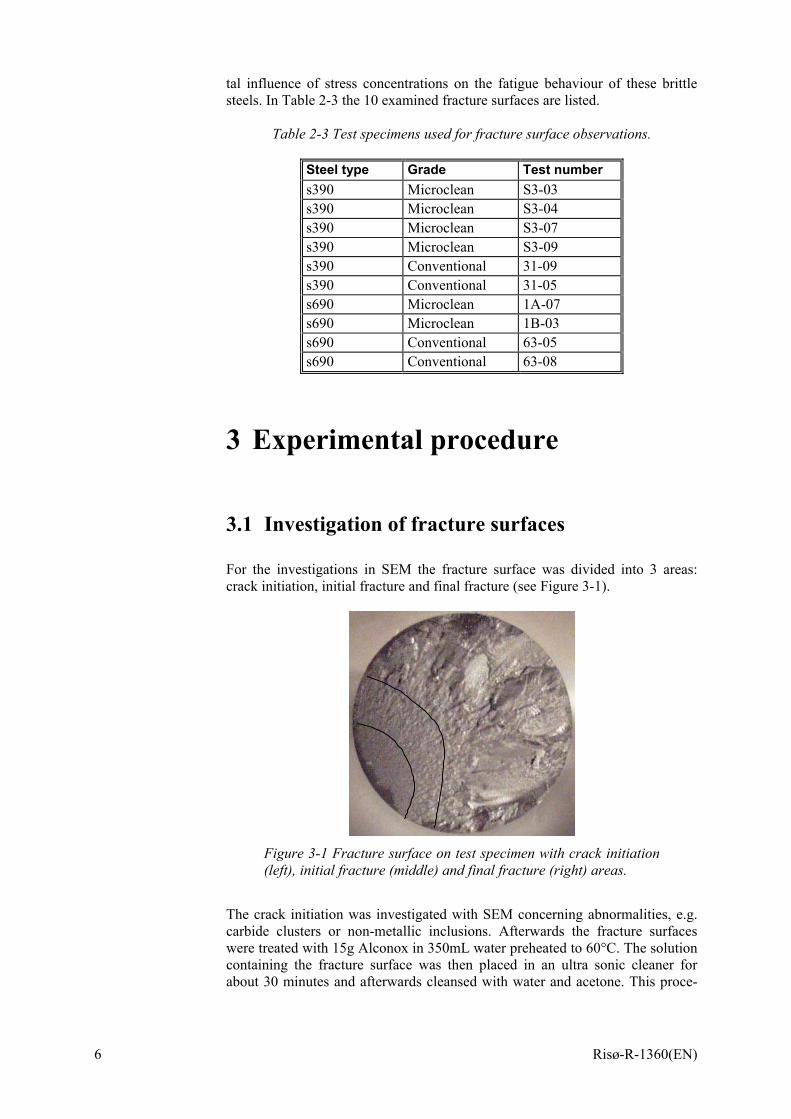
tal influence of stress concentrations on the fatigue behaviour of these brittle steels. In Table 2-3 the 10 examined fracture surfaces are listed.

Table 2-3 Test specimens used for fracture surface observations.

Steel type Grade Test number s390 Microclean S3-03 s390 Microclean S3-04 s390 Microclean S3-07 s390 Microclean S3-09 s390 Conventional 31-09 s390 Conventional 31-05 s690 Microclean 1A-07 s690 Microclean 1B-03 s690 Conventional 63-05 s690 Conventional 63-08

3 Experimental procedure

3.1 Investigation of fracture surfaces For the investigations in SEM the fracture surface was divided into 3 areas: crack initiation, initial fracture and final fracture (see Figure 3-1).

Figure 3-1 Fracture surface on test specimen with crack initiation (left), initial fracture (middle) and final fracture (right) areas.

The crack initiation was investigated with SEM concerning abnormalities, e.g. carbide clusters or non-metallic inclusions. Afterwards the fracture surfaces were treated with 15g Alconox in 350mL water preheated to 60°C. The solution containing the fracture surface was then placed in an ultra sonic cleaner for about 30 minutes and afterwards cleansed with water and acetone. This proce-

6 Risø-R-1360(EN)

dure is described in more details in [5]. The treated fracture surfaces were then examined in SEM. 5 images were recorded at 5000x magnification in each of the three areas i.e. a total of 150 images. The number of fractured carbides was counted manually on the recorded images. A typical image of the fracture sur-face is shown in Figure 3-2.

Figure 3-2 Typical image of fracture surface used for counting fractured carbides.

3.2 Recording of BSE images from polished cross sections On each of the polished cross sections A, B, G and K, 5 images were recorded at 2000x magnification and an acceleration Voltage of 15kV. These images were later used at quantitative image analysis (QIA).

3.3 Search for non-metallic inclusions The 4 polished cross sections were investigated at 750x magnification and an area of approximately 100 images corresponding to approximately 2.7 mm² was examined. When possible non-metallic inclusions were observed an EDS-map were recorded.

3.4 EDS-mapping The EDS-mapping was performed in the LVSEM and the maps were produced using the program ImagePlus, which is part of the Quest software package de-livered by Thermo NORAN. Two types of carbides have previously been identified in the investigated steels: a M6C type (M=Fe, W, Mo) and a V8C7 type [2,3]. For the EDS-maps of the polished cross sections the regions of interest setup were therefore as shown in Figure 3-3 with focus on the elements W, Mo and V. When mapping inclusions additional elements C, O, Al, and Mn were included.

Risø-R-1360(EN) 7

Figure 3-3 ROI-settings in the ImagePlus program.

For the actual mapping of the polished cross sections a resolution of 512x512 and a dwell time of 50 ms was chosen. According to the program, total process time would be approximately 3 hours, but it took only 1½ hours to complete the measurement. For the inclusions a resolution of 256x256 and a dwell time of 10 ms were used. The exact settings for the mapping of the polished cross sections can be seen in Figure 3-4.

8 Risø-R-1360(EN)

Figure 3-4 Map settings in the ImagePlus program.

3.5 Quantitative image analysis (QIA) of EDS-maps QIA was performed using the program Image Pro Plus produced by Media Cy-bernetics. An EDS-map from a polished cross section was loaded into the pro-gram and the image was converted into grey scale 8 (Edit → Convert To → Grey Scale 8), and the threshold function (Process → Threshold…) was run with auto settings (see Figure 3-5).

Risø-R-1360(EN) 9

Figure 3-5 (left) Threshold function in the Image Pro Plus pro-gram. (right) Image map after using the threshold function.

In order to remove disturbing background a median filter was applied with set-tings that can be seen from Figure 3-6.

Figure 3-6 (left) Settings for the applied median filter for removing background noise. (right) Image map after applying the filter.

Now the mean diameter and the area distribution of the particles could be meas-ured with the Measure → Count/Size function (see Figure 3-7).

Figure 3-7 Count/Size window.

10 Risø-R-1360(EN)

Measure → Select Measurements… was chosen and either Diameter (mean) or Per-Area could be selected. The two measurements should not be performed simultaneously, since different border conditions should be applied for the two measurements. Figure 3-8 illustrates the different border conditions, which was selected by pressing Options in the Count/Size window (Figure 3-8). “All borders” were selected for the mean diameter measurement, while “None” was selected if the area distribution was to be measured (Per Area).

Figure 3-8 (left) Settings for mean diameter measurements, parti-cles lying on the borders are not included in the measurements. (right) Settings for Per-Area measurement, all particles are in-cluded.

After applying the correct settings, Count was pressed in the Count/Size win-dow seen in Figure 3-7. The objects were split up and marked automatically and thereafter counted. It can be necessary to further spilt up some of the ob-jects, which could be done by using the function Edit → Split Objects… The objects could be edited and split up into minor objects where this seems appro-priate, viewing the original image while doing this eased this task considerably. Figure 3-9 shows a map, where further splitting of the objects was necessary.

Figure 3-9 Image map during manual splitting of particles.

Risø-R-1360(EN) 11

When this had been done in a satisfactory manner, the measurement data were exported to excel by selecting View → Measurement Data in the Count/Size window and File → DDE to Excel in the Measurement Data window (Figure 3-10). The same could be done for the statistics data (View → Statistics, File → DDE to Excel).

Figure 3-10 Measurement data window.

3.6 Quantitative image analysis (QIA) of BSE im-ages A BSE image was loaded into Image Pro Plus and spatial calibration was per-formed by Measure → Calibration → Spatial then selecting Image at Pix-els/Unit and adjusting the marker. An area of interest (AOI) was marked by clicking NEW AOI and marking the desired area. Now the mean diameter and the area distribution of the bright particles ( (W,Mo)6C-carbides) could be measured with the Measure → Count/Size function (see Figure 3-7). The same measurement setup as described in section 4.3 was chosen. By selecting Select Ranges the threshold/segmentation window appear. The range selected starts where the signal rises from the background and ends at maximum (255) (Figure 3-11).

12 Risø-R-1360(EN)

Figure 3-11 Selection of count range.

After closing the segmentation window, Count was pressed in the Count/Size window seen in Figure 3-7. The measurement data were exported to excel by selecting View → Measurement Data in the Count/Size window and File → DDE to Excel in the Measurement Data window (Figure 3-10). For measurements of the light grey particles (V8C7-carbides) Select Ranges was pressed again and the segmentation window was used to select the grey VC-carbides. To secure reproducibility it was done by selecting the top and adding 8 with the minimum marker, i.e. if the top is at 114 then the marker was placed at 122 (see Figure 3-12). The maximum marker was placed at the bottom and then Transparent on Black chosen and Create Preview Image pressed to create an image consisting only of the selected grey scale.

Figure 3-12 Selection of range for VC-carbides

The segmentation window was closed and Enhance → Equalize→ Best fit was chosen to enhance the contrast. Afterwards a median filter was applied with set-tings that can be seen from Figure 3-6. Then the Count/Size window was opened again (Measure → Count/Size) and Automatic Bright Objects was marked. Then the count was made and the measurement data exported to Excel as described in paragraph 3.5.

Risø-R-1360(EN) 13

The procedure of dividing the carbides was abandoned when performing QIA on BSE images. The reasons for doing so were that it involved a great deal of subjectivity. It was difficult to tell even with the original image besides where to divide (see Figure 3-13).

Figure 3-13 BSE image before (left) and after (right) image proc-essing regarding V8C7-carbides.

The program then counted carbide clusters as one big carbide, this was chosen because carbide clusters affect the material as if it was one big carbide.

14 Risø-R-1360(EN)

4 Results and discussion

4.1 Size distributions

Vanadium carbide size histograms based on BSE images

A s390c

05

1015

0.1 0.5 0.9 1.3 1.7 2.1 2.5 2.9 3.3

E s390c

05

1015

0.1 0.5 0.9 1.3 1.7 2.1 2.5 2.9 3.3

B s690c

05

1015

0.1 0.5 0.9 1.3 1.7 2.1 2.5 2.9 3.3

C s690c

05

1015

0.1 0.5 0.9 1.3 1.7 2.1 2.5 2.9 3.3

J s390m

05

1015

0.1 0.5 0.9 1.3 1.7 2.1 2.5 2.9 3.3

I s390m

0

5

10

15

0.1

0.5

0.9

1.3

1.7

2.1

2.5

2.9

3.3

G s690m

05

1015

0.1 0.5 0.9 1.3 1.7 2.1 2.5 2.9 3.3

H s690m

05

1015

0.1 0.5 0.9 1.3 1.7 2.1 2.5 2.9 3.3

Figure 4-1 Vanadium carbide size histograms based on EDS-maps x-axis: mean diameter in µm; y-axis: frequency in percentage.

Risø-R-1360(EN) 15

The carbide distributions shown in Figure 4-1 are obtained from EDS-maps (see Appendix A). On the EDS-maps the vanadium carbides are colour coded and can easily be distinguished from the matrix, which is a more difficult task on the BSE images (see section 3.6). However, one has to consider the sampling volume that is connected with EDS-mapping. This sampling volume is larger than for backscattered electrons and therefore the BSE images are expected to provide the response closest to a two-dimensional image of the cross-section, while response from deeper lying carbides give rise to increased error in the X-ray maps. Furthermore, the M6C carbides are easier distinguishable from the matrix on the BSE images. Figure 4-2 shows W- and Mo-maps together with the corresponding BSE image. The resolution of the BSE image is clearly supe-rior and a large number of “extra” small carbides present on the W- and Mo-maps are not seen on the BSE image. These are the results of noise and response from deeper lying carbides due to the larger sampling volume of the X-rays.

Figure 4-2 EDS-maps for specimen G after treatment in Image Pro Plus; (left) W-map; (middle) Mo-map; (right) BSE image.

As a consequence of these findings, QIA was performed on BSE-images instead of EDS-maps. Unfortunately it was not possible to extract the VC-carbides from the type 690s steel, because the carbides and the matrix have the same BSE con-trast in this steel.

Vanadium carbide size histograms based on BSE images

Each of the histograms (Figure 4-3) is based on counts from 5 images and car-bides less than 0.1 µm was not taken in consideration. The QIA procedures were created with primary focus on reproducibility and especially regarding the size distribution of the VC-carbides errors occur. The ring shaped structures seen on Figure 3-13 originates because the same grey tones as the VC-carbides are also found around some of the molybdenum/tungsten-carbides. There was not enough contrast difference between the underlying matrix and the VC-carbides to avoid this problem. Therefore a comparison of the results based on X-ray maps and BSE images is not possible. Figure 4-3 reveals no differences between the microclean and the conventional steel types.

16 Risø-R-1360(EN)

A 390s conventional

0

5

10

15

0,1 0,4 0,7 1 1,3 1,6 1,9 2,2 2,5 2,8 3,1 3,4

K 390s microclean

0

5

10

15

0,1 0,4 0,7 1 1,3 1,6 1,9 2,2 2,5 2,8 3,1 3,4

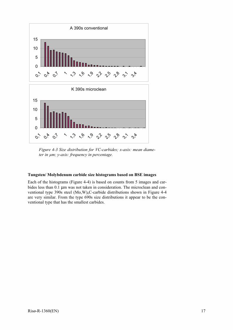
Figure 4-3 Size distribution for VC-carbides; x-axis: mean diame-ter in µm; y-axis: frequency in percentage.

Tungsten/ Molybdenum carbide size histograms based on BSE images

Each of the histograms (Figure 4-4) is based on counts from 5 images and car-bides less than 0.1 µm was not taken in consideration. The microclean and con-ventional type 390s steel (Mo,W)6C-carbide distributions shown in Figure 4-4 are very similar. From the type 690s size distributions it appear to be the con-ventional type that has the smallest carbides.

Risø-R-1360(EN) 17

A 390s conventional

02468

101214

0,1 0,4 0,7 1 1,3 1,6 1,9 2,2 2,5 2,8 3,1 3,4

K 390s microclean

02468

101214

0,1 0,4 0,7 1 1,3 1,6 1,9 2,2 2,5 2,8 3,1 3,4

B 690s conventional

0

2

4

6

8

10

12

14

0,1 0,3 0,5 0,7 0,9 1,1 1,3 1,5 1,7 1,9 2,1 2,3 2,5 2,7 2,9 3,1 3,3 3,5

G 690s microclean

0

2

4

6

8

10

12

14

0,1 0,3 0,5 0,7 0,9 1,1 1,3 1,5 1,7 1,9 2,1 2,3 2,5 2,7 2,9 3,1 3,3 3,5

Figure 4-4 Size distribution for (Mo,W)6C-carbides; x-axis: mean diameter in µm; y-axis frequency in percentage.

18 Risø-R-1360(EN)

4.2 Per area calculation

Vanadium per-area calculation based on EDS-maps

0

0.02

0.04

0.06

0.08

0.1

0.12

0.14

A s390c

E s390c

D s590c

F s590c

B s690c

C s690c

I s390m

J s390m

G s690m

H s690m

VC fr

actio

n of

tota

l are

a

Figure 4-5 Area fraction of VC-carbides based on EDS-maps.

Vanadium per-area calculation based on BSE images

0

0,02

0,04

0,06

0,08

0,1

0,12

K 390s microclean A 390s conventional

VC fr

actio

n of

tota

l are

a

Figure 4-6 Area fraction of VC-carbides based on BSE images.

Risø-R-1360(EN) 19

Tungsten/Molybdenum per-area calculation based on BSE images

0

0,01

0,02

0,03

0,04

0,05

0,06

K 390smicroclean

A 390sconventional

G 690smicroclean

B 690sconventional

(W,M

o)6C

frac

tion

of to

tal a

rea

Figure 4-7 Area fraction of (W,Mo)6-carbides based on BSE images.

The per-area distributions for the two manufacturing types microclean and con-ventional are approximately the same, but there appear to be a larger per-area fraction of M6C carbides in the grade 690s steel.

4.3 Non-metallic inclusions In order to quantify the contents of non-metallic inclusions large areas (2.5-3 mm2 in total) were scanned on polished cross sections of different specimens. When an inclusion was spotted an EDS-map was conducted to identify its com-position. All non-metallic inclusions found on the polished cross sections were different types of oxides containing the following elements: Al, Mn, Mo and W. The quantitative results are shown in Table 4-1, and some examples are shown in Figures 4-8 and 4-9.

Specimen Number of inclu-sions per specimen

inclusions per mm²

K 390s microclean 2 0.7 A 390s conventional 4 1.5 G 690s microclean 3 1,1 B 690s conventional 6 2,2

Table 4-1 Number of inclusions found and estimated number of in-clusion per area.

Although the results shown in Table 4-1 are based on a slim statistic, the ten-dency is clear: the microclean specimens contain less non-metallic inclusions than conventional specimens.

20 Risø-R-1360(EN)

5 µm

Figure 4-8 BSE image (top left) and EDS-maps of inclusion: Al (top right) and O (bottom left).

Figure 4-9 BSE image (top left) and EDS-maps of inclusion: Al (top right),O (bottom left) and W (bottom right).

Risø-R-1360(EN) 21

Figure 4-10 BSE image (left) and SE image (right) of hole from non-metallic inclusion, specimen K.

Figure 4-10 show what is believed to be a hole from one or two inclusions that probably fell out during the grinding process. Small cracks appear in the area around the inclusions as well as within the inclusions. The cracks have not grown beyond the limits of the inclusions, but this is because the polished cross section originate from the thread. If these inclusions had been located in the gauge area during the fatigue testing it would probably have caused the fracture to originate from it. It should be stated, that this observation is unique. All other inclusions resemble those depicted in Figure 4-8 and Figure 4-9. Non-metallic inclusions are without doubt present in the test specimens, but the investigations of the 10 fracture surfaces show no inclusions in the crack initia-tion area. The fact that the fracturing of the specimens occur in the same loca-tion suggest the role played by the non-metallic inclusions are of less impor-tance than the stress concentration of 0.3 percent. In practical applications such a stress concentration is rarely avoided, and often the stress concentration will be much higher. Thus, non-metallic inclusions have little influence on the fa-tigue properties of these steels.

4.4 Fracture surfaces As described in section 3.1 the fracture surfaces were divided into three regions: crack initian area, initial fracture and final fracture (see Figure 3-1). The number of fractured carbides was counted within each of these regions in order to reveal any possible differences in densities of fractured carbides. When counting frac-tured carbides manually, a certain amount of subjectivity will be present. The same criteria for determining whether a carbide is cracked or not, has been ap-plied for all of the images recorded, which give the relative numbers credibility. Thus, any differences between the three regions should be spotted with this method. The results are given in the histograms on the next pages. The histograms show that there are no clear differences in densities of fractured carbides, neither be-tween the three regions nor between the different steel grades. As expected, this suggests that the deformation has been homogeneously distributed in the gauge volume.

22 Risø-R-1360(EN)

Entire sample area

0,000

0,005

0,010

0,015

0,020

0,025

0,030

0,035

0,040

0,045

390s

micr

oclea

n 03

390s

micr

oclea

n 04

390s

micr

oclea

n 07

390s

micr

oclea

n 09

390s

isom

atrix

09

390s

isom

atrix

05

690s

micr

oclea

n 1A-07

690s

micr

oclea

n 1B-03

690s

isom

atrix

05

690s

isom

atrix

08

Cra

cked

car

bide

s pe

r squ

are

mic

rom

eter

VanadiumMolybdæn/WolframTotal

Figure 4-11 Average numbers of cracked carbides per µm² on the entire sample area.

Crack initiation

0,000

0,005

0,010

0,015

0,020

0,025

0,030

0,035

0,040

0,045

390s

micr

oclea

n 03

390s

micr

oclea

n 04

390s

micr

oclea

n 07

390s

micr

oclea

n 09

390s

isom

atrix

09

390s

isom

atrix

05

690s

micr

oclea

n 1A-07

690s

micr

oclea

n 1B-03

690s

isom

atrix

05

690s

isom

atrix

08

Cra

cked

car

bide

s pe

r squ

are

mic

rom

eter

VanadiumMolybdæn/WolframTotal

Figure 4-12 Average numbers of cracked carbides per µm² on the crack initiation region.

Risø-R-1360(EN) 23

Fracture initiation

0,000

0,005

0,010

0,015

0,020

0,025

0,030

0,035

0,040

0,045

390smicroclean

03

390smicroclean

04

390smicroclean

07

390smicroclean

09

390sisomatrix

09

390sisomatrix

05

690smicroclean

1A-07

690smicroclean

1B-03

690sisomatrix

05

690sisomatrix

08

Cra

cked

car

bide

s pe

r squ

are

mic

rom

eter

VanadiumMolybdæn/WolframTotal

Figure 4-13 Average numbers of cracked carbides per µm² in the initial fracture region.

Final fracture

0,000

0,005

0,010

0,015

0,020

0,025

0,030

0,035

0,040

0,045

390smicroclean

03

390smicroclean

04

390smicroclean

07

390smicroclean

09

390sisomatrix

09

390sisomatrix

05

690smicroclean

1A-07

690smicroclean

1B-03

690sisomatrix

05

690sisomatrix

08

Cra

cked

car

bide

s pe

r squ

are

mic

rom

eter

VanadiumMolybdæn/WolframTotal

Figure 4-14 Average numbers of cracked carbides per µm² in the final fracture region.

24 Risø-R-1360(EN)

5 Conclusions When comparing the carbide size distributions of the grade 390s conventional and the microclean tool steel no differences are observed. In the grade 690s the microclean contain fewer small (0.1-0.6 µm) carbides than by the conventional. Mutually the 390s and 690s contain the same area fraction of carbides regard-less of manufacturing method. The non-metallic inclusions are present in the extent illustrated in Table 4-1. The microclean specimens contain less non-metallic inclusions than conven-tional specimens. Also the 690s specimens contain more non-metallic inclu-sions than the 390s specimens. The investigations of fracture surfaces indicate that there are no differences in densities of fractured carbides between the different types of steel or in the spa-tial distribution. No link between non-metallic inclusions and the crack initia-tion were found.

6 References 1. C. Højerslev (2001). Tool steels. Risø Report No. R-1244(EN), Risø Natio-

nal Laboratory, Roskilde, Denmark.

2. C. Højerslev, J.V. Carstensen, P. Brøndsted, M.A.J. Somers (2002). Fatigue Crack Behaviour in a High Strength Tool Steel. In: Proceedings of the 8th International Congress on Fatigue, EMAS, Stockholm.

3. C. Højerslev, J.V. Carstensen, P. Brøndsted, M.A.J. Somers (2001). Resid-ual stresses in a M3:2 PM high speed steel; effect of mechanical loading. In: Proceedings of the 7th International Conference on Advanced Materials and Processes, EUROMAT, Rimini.

4. http://www.bohler-edelstahl.at

5. K.V. Dahl (2002). Fractography analysis of tool samples used for cold forging, Risø Report No. R-1359(EN), Risø National Laboratory, Roskilde, Denmark.

Risø-R-1360(EN) 25

Appendix A: Images of polished cross sections

Specimen A

Figure A-1 (left) EDS-map of specimen A made using the autogroup function, Mo: blue, W: green, V: red. (right) BSE im-age.

Specimen B

Figure A-2 (left) EDS-map of specimen B made using the autogroup function, Mo: blue, W: green, V: red. (right) BSE im-age.

26 Risø-R-1360(EN)

Specimen C

Figure A-3 (left) EDS-map of specimen C made using the autogroup function, Mo: blue, W: green, V: red. (right) BSE im-age.

Specimen E

Figure A-4 (left) EDS-map of specimen E made using the autogroup function, Mo: blue, W: green, V: red. (right) BSE im-age.

Risø-R-1360(EN) 27

Specimen G

Figure A-5 (left) EDS-map of specimen G made using the autogroup function, Mo: blue, W: green, V: red. (right) BSE im-age.

Specimen H

Figure A-6 (left) EDS-map of specimen H made using the autogroup function, Mo: blue, W: green, V: red. (right) BSE im-age.

28 Risø-R-1360(EN)

Specimen I

Figure A-7 (left) EDS-map of specimen I made using the autogroup function, Mo: blue, W: green, V: red. (right) BSE image.

Specimen J

Figure A-8 (left) EDS-map of specimen J made using the autogroup function, Mo: blue, W: green, V: red. (right) BSE im-age.

Risø-R-1360(EN) 29

Bibliographic Data Sheet Risø-R-1360(EN) Title and authors Analysis of carbides and inclusions in high speed tool steels Kasper Tipsmark Therkildsen and Christian Vinter Dahl ISBN ISSN 87-550-3105-6; 87-550-3106-4 (Internet) 0106-2840 Department or group Date Materials Research Department August 2002 Groups own reg. number(s) Project/contract No(s) Sponsorship Pages Tables Illustrations References 30 4 36 5 Abstract (max. 2000 characters) The fracture surfaces of fatigued specimens were investigated using scanning electron microscopy (SEM) and energy dispersive x-ray spectroscopy (EDS). The aim was to quantify the distribution of cracked carbides and non-metallic inclusions on the fracture surfaces as well as on polished cross sections. The specimens were made of Böhler P/M steel grade 390s and 690s in both micro-clean and conventional grades. The results show that the content of non-metallic inclusions are higher in the conventional grades than in the microclean grades, but there were found to be no link between non-metallic inclusions and the crack initiation. Surprisingly, no differences were found between the carbide size distributions of the micro-clean and conventional grades. Also, the distribution of the fractured carbides was found to be the same regardless of steel type, manufacturing method or lo-cation on the specimen. Descriptors INIS/EDB