analysis and scaling of coupled neutronic thermal
TRANSCRIPT

Analysis and Scaling of Coupled Neutronic
Thermal Hydraulic Instabilities of
Supercritical Water-Cooled Reactor
Thesis Submitted in Partial Fulfilment of the Requirements
for the Degree of Doctor of Philosophy
by
DAYA SHANKAR
DEPARTMENT OF MECHANICAL ENGINEERING
INDIAN INSTITUTE OF TECHNOLOGY GUWAHATI

TH-1888_11610303

i
CERTIFICATE
It is certified that the work contained in this thesis entitled Analysis and
Scaling of Coupled Neutronic Thermal Hydraulic Instabilities of
Supercritical Water-Cooled Reactor by Daya Shankar, research scholar in
the Department of Mechanical Engineering, Indian Institute of Technology
Guwahati, India, toward the award of the degree of Doctor of Philosophy, has
been carried out under our joint supervision, and that this work has not been
submitted elsewhere for a degree.
Dr. Manmohan Pandey
Professor
Department of Mechanical
Engineering, Indian Institute of
Technology Guwahati, Assam, India
8th October 2018
Dr. Dipankar N. Basu
Assistant Professor
Department of Mechanical
Engineering, Indian Institute of
Technology Guwahati, Assam, India
8th October 2018
TH-1888_11610303

ii
TH-1888_11610303

iii
DECLARATION
I declare that the work contained in this thesis entitled Analysis and Scaling
of Coupled Neutronic Thermal Hydraulic Instabilities of Supercritical
Water-Cooled Reactor, submitted toward the award of the degree of Doctor
of Philosophy, has been carried out by me under the joint supervision of Dr.
Manmohan Pandey and Dr. Dipankar N. Basu, and that this work has not
been submitted elsewhere for a degree.
Daya Shankar
Research Scholar
Department of Mechanical
Engineering, Indian Institute of
Technology Guwahati, Assam, India
8th October 2018
TH-1888_11610303

iv
TH-1888_11610303

v
ACKNOWLEDGEMENTS
First, I would like to thank my doctoral advisors, Dr. Manmohan Pandey and
Dr. Dipankar Narayan Basu, for their exceptional guidance, expertise, and
patience over the years. Their consistent encouragement has helped me make
this thesis a work I can be truly proud of. I am immensely grateful to them for
providing me with the opportunity to do this research and develop my skills
in a field, which has both fundamental scientific value and current practical
relevance. Their kindness and grace always gave me determination and will
to work.
I wish to express my warm and sincere thanks to my doctoral committee
members Late. Prof. Subhash C. Mishra, Prof. Anoop K. Dass, Dr. Anugrah
Singh and Dr. Ganesh Natarajan, for giving their valuable suggestions and
encouragement during my research work.
I am extremely grateful to IIT Guwahati for providing me with the financial
support during the course of my PhD. I would also like to acknowledge all the
necessary infrastructure offered by Department of Mechanical Engineering,
IIT Guwahati requisite for the smooth running of my research work. I am
thankful to all the faculty members and staff members of Department of
Mechanical Engineering, IIT Guwahati who helped me in different ways
whenever I had any problem.
I would like to recognize the many friends I have made since coming to IIT for
their camaraderie and their contributions intentional or otherwise to this
thesis. I would like to thank Dr. Vijay Kumar Mishra, Dr. Jai Manik, Milan
Krishna Singha Sarkar, Kiran Shakia, A Srinivas Pavan Kumar, Ashif Iqbal,
Sandeep Sharma and many others for all the supreme times, and for likely
extending the amount of time it took to complete the work contained in this
thesis.
TH-1888_11610303

vi
Of course, none of this would have been possible without the love of my family;
particularly my parents: Smt. Geeta Devi and Shri P.N.Tiwary and. Their life-
long support and encouragement has contributed so much to making me who
I am, and I simply cannot thank them enough for everything they have done
for me.
I reserve my heart full of affection and sincere gratitude to my wife Dr. Beauty
Pandey for her love, motivations, patience and inspirations during my
research work. I take this opportunity to appreciate and thank her for the
hardship she had undergone during the stressful moments of my research
work.
I take this opportunity to express my sincere thanks to Dr. Shraddha Basu
for her kind hospitality and concern during our tough times. I would also like
to thanks Smt. Divya Pandey for her indirect support. I extend my blessings
and wishes to Baby Eirene and Master Subham Pandey. I wish both of them
a glorious and prosperous future.
I would also like to thanks Prof. Biplab Halder for their encouragement and
motivation.
Lastly, I would like to thank the Almighty without whose blessings and
strength nothing would had been possible. Thank You Maa Kamakhya, for
everything!!
All these contributions through every aspect of my life is pre and post Ph.D
can never be expressed in words.
I would also like to apologise if I have missed any name. All your contribution
all immensely valuable.
Thank you everyone.
Daya Shankar
October 2018
TH-1888_11610303

vii
ABSTRACT
Present thesis work primarily focuses on the analysis of flow instability
in one of the most powerful concepts under Generation-IV nuclear reactors;
technology, namely, Supercritical water-cooled reactor (SCWR). Safety is the
primary concern in the any nuclear reactors. Flow instabilities are one of a
kind on which the current researches are going on. The reason behind that is
the large density difference of the fluid through the coolant channel.
Therefore, a downscaled model is required to study the complex phenomena
in laboratory conditions; hence a scaled method is proposed here which is
useful for the study of both the natural as well as the forced circulation
system. For further analysing about the stability of the system, a simple but
quite effective model has been developed as the Lumped Parameter Model
(LPM). Using this model, a linear and nonlinear stability analysis have been
done for the various parametric conditions. Moreover, the stability analysis
due to the seismic effects on SCWR has also been considered by using the
same LPM. Two types of seismic wave model have been taken into account for
the analysis, first the sinusoidal acceleration and the other more realistic
Kanai–Tajimi model which is used for more accurate simulation of the seismic
wave. These methods are first time introduced in the SCWR.
Nuclear power plants use the heat generated from nuclear fission in a
contained environment to convert water into steam, which further utilized for
electricity production. The concept of nuclear power generation had started
in 1950. According to European Nuclear Society (www.euronuclear.org), as of
November 28, 2016, in 31 countries 450 nuclear power plant units with an
installed electric net capacity of about 392 GW are in operation, and 60 plants
with an installed capacity of 60 GW are in 16 countries under construction.
SCWR is a concept for an advanced reactor that operates at supercritical
pressures and temperatures (25–30 MPa, 500-520 oC exit temperature). Such
a high coolant temperature at turbine inlet provides high thermal efficiency
TH-1888_11610303

viii
(~42%) which is substantially higher than any other LWR (~30%). But this is
on the cost of large density difference throughout the coolant channel, from
the inlet to the outlet (720 kg/m3 to 90 kg/m3), which raises a serious concern
about flow instabilities in the SCWR. To ensure a proper design of the reactor
without any sustainability issue, detailed stability analysis is essential.
It is evident from a meticulous survey of the relevant literature that, while the
natural circulation-based systems have received some attention, supercritical
channels with the forced flow generally experience a more considerable
density variation across the core could not grab the proper attention of the
researcher which is also more susceptible towards thermohydraulic
instabilities. So, for the study and analysis of the latter system, a lumped
parameter-based approach is followed.
The lumped parameter model (LPM) is derived from the basic governing
equations of mass, momentum and energy. The basic governing equations,
which are in PDE form, can be transformed into an equivalent nonlinear
system of ODEs by nodalization and spatial integration. As LPM is
computationally inexpensive, hence it is suitable for detailed parametric
studies of stability trends. The general transient equations are difficult to
solve because of the coupling between the momentum and energy equations
and the nonlinear nature of these general equations. Therefore, in the present
model Channel Integral (CI) method is used. The integrations of the
conservation equations are done over first and second zone of the flow channel
respectively, and the resultant system of algebraic and ODEs are employed
for both linear and nonlinear analysis.
The Scaling of SCWR system is primely done for identifying a less restrictive
model fluid, which can adequately mimic the SCW under the relevant scaled
condition of an SCWR, and to define the scaling rules in a generalized way, to
preserve the phenomenological physics. The focus is kept on uncoupling the
radial scaling from the axial one, as only then a possible combination of
system dimensions can be proposed.
TH-1888_11610303

ix
US reference design of SCWR (Zhao et al., 2007) is considered as the
prototype. Accordingly, the scaled dimensions of the lab-scale facility and
corresponding operational settings regarding power, flow rate, and inlet
temperature are proposed. The advantages of the proposed methodology over
the existing ones have also been stressed upon, along with a discussion on
the role of involved dimensionless groups.
A circular forced flow channel of uniform diameter is simulated in the present
study, with uniform heat flux on the wall. The channel is subjected to both
constant pressure drops and constant mass flow rate boundary conditions for
the analysis. The one-dimensional conservation equations for mass,
momentum, and energy have been taken. For the sake of generalizations,
governing equations are nondimensionalized using the suitable dimensionless
parameters. The equations for mass and energy are integrated over the first
node, i.e., from inlet until the appearance of the pseudocritical point.
Correspondingly, two ODEs can be obtained in terms the location of
pseudocritical boundary. Now, again integrating the conservation equations
over the second node, from the pseudocritical point to the channel outlet, two
ODEs are achieved in terms of the outlet enthalpy. These four equations are
sufficient for the mass flow rate boundary condition. However, for pressure-
drop, boundary condition, the equation for conservation of momentum is
integrated separately over both the zones and added to represent the net
pressure drop across the channel. Accordingly, the six ODEs are selected for
analysis, along with algebraic equations which are obtained by equating the
ODE’s of mass and energy equations for the two zones, and the equation of
state. In order to capture the sharp variation in thermophysical properties of
supercritical water around the pseudocritical point, the equation of state is
replaced by fitting a separate rectangular hyperbola for each of the zones.
In order to introduce the power dynamics into framework, mathematical
model for point reactor kinetics and a lumped parameter representation of the
energy balance across the fuel rod are taken into consideration. The heat
TH-1888_11610303

x
generated inside the fuel rod is convectively transferred to the coolant from
the rod surface. Applying energy balance with lumped capacitance
approximation for the fuel rod, the state equation for fuel temperature and
coolant enthalpy can be expressed in non-dimensional form. Therefore, the
initial system of PDEs gets converted to a set of algebraic equations and
ODEs, with dimensionless time as the sole independent variable. Finally, the
thermal hydraulic part is compared with RELAP and found that the LPM
results are more conservative than those predicated by RELAP, which implies
that the use of LPM for stability analysis is safe. In addition to this, stability
map for the various geometric and neutronic parameters have been generated.
Based on the motivation from the two-zone model, a three-zone model has
been studied for the stability analysis. The whole flow region is divided as
heavy fluid region (H-F), heavy & light fluid mixture region (H-L-M) and light
fluid region (L-F) following the approach proposed by Zhao (2007). After
analysing the results, within ±10 % increases in the stability boundary has
been observed, which do not justify the complexity of the formulations. The
qualitative behaviour of both the models are similar, hence it is recommended
that for the preliminary stability analysis, two zone model is more justified
then the three-zone model.
The linear stability of SCWR channels has been studied in past. However, the
analysis is valid only for infinitesimally small perturbations. Therefore, there
is a need to carry out stability analysis for small finite sized perturbations.
Moreover, earlier studies do not consider inclination of these channels, which
exist for various applications. The present thesis work has also attempted
linear, as well as nonlinear, stability analysis of the channel. The bifurcation
analysis is carried out to capture the nonlinear dynamics of the system and
to identify regions in the parameter space for which subcritical and
supercritical bifurcations exist. The study is carried out for different
inclination angles in order to characterize the effect of inclination on the
stability of the system. The analysis shows that, at all conditions, a
TH-1888_11610303
xi
generalized Hopf point exists. The subcritical and supercritical bifurcations
are confirmed by numerical simulation of the time-dependent, nonlinear
ODEs for the selected points in the operating parameter space. The
identification of these points is important because the stability characteristics
of the system for finite perturbations are dependent on them. Both stable and
unstable limit cycle has been detected and the boundaries of the unstable
limit cycle have also been calculated.
In the SCWR subjected to an earthquake, the oscillating acceleration
attributable to the seismic wave may cause the variation of the coolant flow
rate and density reactivity in the core, which might result in the core
instability due to the density-reactivity feedback. Therefore, it is important to
properly evaluate the effect of the seismic acceleration on the core stability
from a viewpoint of plant integrity estimation. In this study, the in-house code
using LPM two zone model is employed for stability appraisal under the
seismic acceleration, considering the one-dimensional neutron-coupled
thermal hydraulic equations. The coolant flow in the core is simulated by
introducing the oscillating acceleration attributed to the earthquake motion
into the momentum equation as external force terms. Both a simple periodic
acceleration and the acceleration obtained from the response analysis to the
El Centro seismic wave of Imperial Valley earthquake. An artificial earthquake
records with a nonstationary Kanai–Tajimi model is also used for more
accurate simulation of the earthquake. Finally, the behaviours of the core and
coolant are calculated in terms of various parameters of acceleration. The
effects of the neutronics, amplitude, and direction of the oscillating
acceleration have been discussed. The stability map has been plotted based
on these pieces of information.
TH-1888_11610303

xii
TH-1888_11610303

xiii
CONTENTS
CERTIFICATE............................................................................................ i
DECLARATION ........................................................................................ iii
ACKNOWLEDGEMENTS ........................................................................... v
ABSTRACT ............................................................................................. vii
CONTENTS ........................................................................................... xiii
NOMENCLATURE .................................................................................. xix
LIST OF FIGURES ................................................................................ xxii
LIST OF TABLES .................................................................................. xxvi
INTRODUCTION.................................................................... 1
1.1 Motivation ..................................................................................... 1
1.2 Classification of flow instability ...................................................... 7
1.2.1 Static instability ...................................................................... 7
1.2.2 Dynamic instabilities ............................................................... 9
1.2.3 Coupled neutronics instabilities ............................................. 13
1.3 Mathematical modelling ............................................................... 14
1.4 Theoretical analysis of instability ................................................. 14
1.4.1 Real time analysis .................................................................. 14
1.4.2 Linear stability analysis ......................................................... 15
1.4.3 Nonlinear stability analysis .................................................... 16
1.5 Instability due to seismic effect .................................................... 17
1.6 Research objectives ..................................................................... 18
1.7 Outline of the thesis .................................................................... 18
LITERATURE REVIEW......................................................... 22
2.1 Instability in SCWR ..................................................................... 22
TH-1888_11610303

xiv
2.2 Instability in BWR ....................................................................... 36
2.3 Scaling for instability of fluid in SCWR ......................................... 38
2.4 Mathematical modelling ............................................................... 46
2.5 Seismic effect on flow instability ................................................... 56
2.6 Observation from literature survey ............................................... 58
MATHEMATICAL MODELLING............................................. 62
3.1 Introduction ................................................................................ 62
3.2 Lumped parameter model ............................................................ 64
3.2.1 Thermal-hydraulic modelling .................................................. 66
3.2.2 Fuel dynamics ....................................................................... 68
3.2.3 Power dynamics ..................................................................... 69
3.3 Steady-state equations ................................................................ 72
3.3.1 Comparison of steady state results ......................................... 73
3.4 Transient equations ..................................................................... 74
3.4.1 Pressure drop boundary condition .......................................... 75
3.4.2 Mass flow rate boundary condition ......................................... 77
3.5 RELAP model .............................................................................. 78
3.5.1 Nodal sensitivity test .............................................................. 80
3.5.2 Comparison of LPM and RELAP5 ............................................ 81
3.6 Validation of LPM with the experimental result ............................. 83
3.7 Stability analysis ......................................................................... 87
3.7.1 Linear stability analysis ......................................................... 87
3.7.2 Non-linear stability analysis ................................................... 89
SCALING METHODOLOGY FOR STABILITY APPRAISAL ........ 92
4.1 Introduction ................................................................................ 92
TH-1888_11610303

xv
4.2 Fluid-to-fluid scaling methodology................................................ 93
4.2.1 Conservation equations .......................................................... 93
4.2.2 Scaling principles .................................................................. 94
4.3 Selection of fluids ........................................................................ 95
4.3.1 Scaling rules.......................................................................... 96
4.3.2 Pressure ................................................................................ 96
4.3.3 Length of the channel ............................................................ 96
4.3.4 Mass flux .............................................................................. 96
4.3.5 Hydraulic diameter ................................................................ 97
4.3.6 Power and inlet temperature................................................... 97
4.4 Results and discussion ................................................................ 98
4.4.1 Comparison with existing scaling method................................ 99
4.4.2 Comparison of different model fluids ..................................... 100
4.4.3 Generalized stability map ..................................................... 101
4.4.4 Transient analysis of R-134a ................................................ 103
4.5 Conclusions .............................................................................. 108
PARAMETRIC EFFECTS ON STABILITY CHARACTERISTICS
111
5.1 Introduction .............................................................................. 111
5.2 Mathematical modelling ............................................................. 112
5.3 Results and discussion .............................................................. 113
5.3.1 Transients simulations ......................................................... 116
5.3.2 Parametric effects on pure thermal hydraulic stability ........... 118
5.3.3 Coupled neutronics-thermal hydraulic stability ..................... 123
5.4 Conclusions .............................................................................. 126
TH-1888_11610303

xvi
STABILITY ANALYSIS OF SCWR USING THREE ZONE LPM 129
6.1 Introduction .............................................................................. 129
6.2 Mathematical modelling ............................................................. 131
6.2.1 Equations of state (EOS) ...................................................... 132
6.2.2 Enthalpy profile and relation between 𝝆 ∗ and 𝒉 ∗ .................. 133
6.3 Results and discussion .............................................................. 136
6.3.1 Effect of length .................................................................... 139
6.3.2 Effect of hydraulic diameter .................................................. 140
6.3.3 Effects of orifice coefficients .................................................. 141
6.4 Comparisons of two-zone and three-zone model .......................... 143
6.5 Conclusions .............................................................................. 143
NONLINEAR DYNAMICS AND BIFURCATION ANALYSIS ..... 146
7.1 Introduction .............................................................................. 146
7.2 Mathematical modelling ............................................................. 147
7.3 Results and discussion .............................................................. 147
7.3.1 Identification of generalized Hopf (GH) points ........................ 147
7.3.2 Numerical simulation analysis in supercritical region ............ 150
7.3.3 Numerical simulation analysis in subcritical region ............... 151
7.4 Analysis of neutronics and geometrical parameters ..................... 152
7.4.1 Effect of fuel time constant: .................................................. 152
7.4.2 Effect of the density reactivity constant: ................................ 153
7.4.3 Effect of the length area ratio:............................................... 154
7.4.4 Effect of the mass flow rate:.................................................. 155
7.5 Conclusions .............................................................................. 155
TH-1888_11610303

xvii
NEUTRONICS-COUPLED THERMAL HYDRAULIC
CALCULATION OF SCWR UNDER SEISMIC WAVE ACCELERATION ....... 158
8.1 Introduction .............................................................................. 158
8.2 Technique & methods ................................................................ 160
8.3 Input model .............................................................................. 161
8.4 Modelling of seismic acceleration: ............................................... 162
8.5 Results and discussion .............................................................. 164
8.5.1 Sensitivity calculations on the degree of stability and amplitude of
acceleration: .................................................................................. 164
8.5.2 Neutronics behaviour ........................................................... 165
8.6 Kanai–Tajimi model ................................................................... 170
8.7 Simulation of ground acceleration record .................................... 172
8.7.1 Effect of density reactivity constant....................................... 172
8.8 Conclusions .............................................................................. 175
SUMMARY AND CONCLUSIONS ........................................ 178
9.1 Summary .................................................................................. 178
9.2 Conclusions .............................................................................. 181
9.3 Future works ............................................................................ 182
LIST OF PUBLICATIONS ....................................................................... 186
Journals ........................................................................................... 186
Conferences ...................................................................................... 186
APPENDIX-A ........................................................................................ 188
Flow chart of stability analysis of SCWR ............................................. 188
REFERENCES ...................................................................................... 190
TH-1888_11610303

xviii
TH-1888_11610303

xix
NOMENCLATURE
𝐴 Area (m2)
𝐶 Precursor density (cm-3)
𝐶𝑓 Heat capacity of fuel rod (kJ K-1)
𝐶𝑝 Isobaric specific heat (kJ kg-1 K-1)
𝐷ℎ Hydraulic diameter (m)
𝑓 Friction factor (–)
𝑔 Gravitational acceleration (m s-2)
𝐺 Mass flux (kg m-2 s-1)
ℎ Enthalpy (kJ kg-1)
𝑘 Feedback reactivity (–)
𝐾 Restriction coefficient (m-1)
𝐿 Core length (m)
𝑛𝑓 Number of fuel rods (–)
𝑁𝐸𝑢 Euler number (–)
𝑁𝐹𝑟 Froude number (–)
𝑁𝑆𝑃𝐶 Pseudo subcooling number (–)
𝑁𝑇𝑃𝐶 Transcritical phase-change number (–)
𝑝 Pressure (N m-2)
𝑃 Power (kW)
𝑞𝑜′′ Heat flux (kW m-2)
𝑡 Time (s)
TH-1888_11610303

xx
𝑇 Absolute temperature (K)
𝑧 Space coordinate (m)
Greek symbols
𝛼 Heat transfer coefficient (kW m-2 K-1)
𝛽̅ Volumetric expansion coefficient (K-1)
𝛽 Delayed neutron fraction (–)
𝛾 Nondimensionalized neutron generation time (–)
𝜌 Density (kg m-3)
𝜎 = 𝛽/𝛾 (–)
𝜋ℎ Heated perimeter (m)
Subscripts
0 Reference
𝑎 Acceleration
𝑐 Core
𝑓 Fuel rod / Friction
𝑔 Gravitational
𝑖 Inlet
𝐿 Loss
𝑜 Outlet
𝑝𝑐 Pseudocritical
∗ Dimensionless quantities
TH-1888_11610303

xxi
TH-1888_11610303

xxii
LIST OF FIGURES
Figure 1-1: Global power generation (https://goo.gl/uDGWgx) .............................. 1
Figure 1-2: Schematics of SCWR (https://goo.gl/qHdFrz) ..................................... 3
Figure 1-3: Pressure vessel type reactor (Source: google) ...................................... 5
Figure 1-4: Pressure tube type reactor (https://goo.gl/G4RChr) ............................ 5
Figure 1-5: Types of flow instability-(Prasad et al. 2007) ........................................ 8
Figure 1-6: Ledinegg instability (Kakac and Bon, 2008) ......................................... 9
Figure 1-7: Different type of Static Instability...................................................... 11
Figure 1-8: Different types of Dynamic Instability ............................................... 12
Figure 3-1: Schematic representation of the channel under consideration ........... 65
Figure 3-2: Comparison of the steady state pressure distribution along the channel
for the single channel obtained by LPM with Ambrosini and Sharabi (2008) ......... 74
Figure 3-3: Comparison of the steady state density distribution along the channel for
the single channel obtained by LPM with Ambrosini and Sharabi (2008) .............. 74
Figure 3-4: Polynomial fitting of IAPWS data for water at 25 MPa .................................... 77
Figure 3-5: Nodalization diagram ....................................................................... 80
Figure 3-6: Nodal sensitivity for three different volumes ...................................... 81
Figure 3-7: Comparisons of LPM with RELAP ................................................... 83
Figure 3-8: Validation of LPM with experimental data (Xi et al. (2014)) ................. 83
Figure 3-9: Comparison of experimental and numerical NTPC .............................. 85
Figure 4-1: Non-dimensional property variation for three fluids at equivalent
pressure levels .................................................................................................. 95
Figure 4-2: Stability map for three fluids following linear stability analysis ........ 102
Figure 4-3: Effect of system pressure on the stability map for (a) water, (b) R134a
and (c) CO2...................................................................................................... 103
Figure 4-4: Linear stability map of R-134a corresponding to 25 and 30 MPa of water
....................................................................................................................... 104
Figure 4-5: Stable response of SCWR corresponding to point ‘a’ in the stability map
at 6.2 MPa system pressure, 800 kg/s mass flow rate and 241.8 MW input power
....................................................................................................................... 106
Figure 4-6: Unstable response of SCWR corresponding to point ‘b’ in the stability
map at 6.2 MPa system pressure, 800 kg/s mass flow rate and 242 MW input power
....................................................................................................................... 107
TH-1888_11610303
xxiii
Figure 5-1: Stability map for water at 25 MPa system pressure ......................... 113
Figure 5-2: Comparisons of stability map at 25 MPa for thermal hydraulic in two
different boundary conditions .......................................................................... 115
Figure 5-3: Variation of Viscosity and density with inlet temperature of water at 25
MPa ................................................................................................................ 115
Figure 5-4: Stable response of SCWR corresponding to point ‘a’ in the stability map
at 25 MPa system pressure, 1843 kg/s mass flow rate and 0.32 MW/Channel input
power .............................................................................................................. 116
Figure 5-5: Neutrally stable response of SCWR corresponding to point ‘b’ in the
stability map at 25 MPa system pressure, 1843 kg/s mass flow rate and 0.35
MW/Channel input power ............................................................................... 117
Figure 5-6: Unstable response of SCWR corresponding to point ‘c’ in the stability map
at 25 MPa system pressure, 1843 kg/s mass flow rate and 3.16 MW/Channel input
power .............................................................................................................. 118
Figure 5-7: Effect of channel length on non-dimensional plain .......................... 119
Figure 5-8: Effect of channel length, Inlet temperature verses power ................. 119
Figure 5-9: Effect of channel hydraulic diameter on non-dimensional plain without
orifice coefficient.............................................................................................. 121
Figure 5-10: Effect of channel hydraulic diameter, Inlet temperature verses power
plain ............................................................................................................... 121
Figure 5-12: Effect of inlet and outlet orifice coefficient stability map ................. 122
Figure 5-13: Effect of inlet and outlet orifice coefficient, Inlet temperature verses
power .............................................................................................................. 123
Figure 5-14: Effect of Fuel time constant at pressure 25MPa and enthalpy reactivity
coefficient is –0.005 ......................................................................................... 125
Figure 5-15: Effect of enthalpy Reactivity Coefficient at pressure 25MPa and fuel time
constant 8 s. ................................................................................................... 125
Figure 6-1: Schematic view of the heated channel following by three-region model
....................................................................................................................... 132
Figure 6-2: Fitting of equation of state with IAPWS data of water at 25 MPa. ...... 133
Figure 6-3: Transient variation of 1st zone boundary in stable region at Ntpc =6.0 and
Nspc =2.24 ...................................................................................................... 138
TH-1888_11610303
xxiv
Figure 6-4: Transient variation of 1st zone boundary on marginal stable boundary
Ntpc =6.13 and Nspc =2.24 .............................................................................. 139
Figure 6-5: Transient variation of 1st zone boundary in unstable region at Ntpc =6.28
and Nspc =2.24 ............................................................................................... 139
Figure 6-6: Stability map of three different channel length. ............................... 140
Figure 6-7: Stability map of three different channel hydraulic diameter. ............ 141
Figure 6-8: Stability map of four different sets of orifices coefficients ................. 142
Figure 6-9: Stability map comparing two- zone and three-zone model. ............... 143
Figure 7-1: Stability map showing GH point on MSB......................................... 148
Figure 7-2: Temporal variation of Zpc*............................................................. 149
Figure 7-3: Temporal variation of Zpc* ............................................................. 149
Figure 7-4: Phase portrait of Go*and Zpc* ........................................................ 150
Figure 7-5: Unstable temporal variation of Zpc* corresponding to point M ......... 150
Figure 7-6: Phase portrait of Gpc* and Zpc* ...................................................... 151
Figure 7-7: Stability map of Fuel time constant at 25MPa at density reactivity
constant 10-5/(kg/m3) ...................................................................................... 152
Figure 7-8: Stability map of density reactivity constant at 25 MPa and fuel time
constant 2s. .................................................................................................... 153
Figure 7-9: Stability map of L/A ratio of system at 25 MPa ................................ 154
Figure 7-10: Comparisons of different mass flow at 25 MPa............................... 155
Figure 8-1: Input power profile distribution at steady state ............................... 161
Figure 8-2: Core power transients after step change in pressure in BWR analysis
....................................................................................................................... 162
Figure 8-3: Peak power height as a function of decay ratio ................................ 165
Figure 8-4: Peak power height as a function of the amplitude of the external
acceleration..................................................................................................... 165
Figure 8-5: Stability map of two different Fuel Time Constants .......................... 166
Figure 8-6: Transient plot of ZPC* in stable zone ................................................ 167
Figure 8-7: Phase portrait of ZPC* vs GPC* in stable zone .................................... 167
Figure 8-8: Transient plot of ZPC* at marginal stable boundary .......................... 168
Figure 8-9: Transients plot of ZPC* in unstable zone .......................................... 168
Figure 8-10: Phase portrait of GPC* vs ZPC* in unstable zone .............................. 169
Figure 8-11: Density reactivity coefficient at fuel time 2 s. ................................. 169
TH-1888_11610303

xxv
Figure 8-12: Transient Ground acceleration plot using Kania-Tajimi power spectral
density ............................................................................................................ 171
Figure 8-13: Fitted envelop on orifinal data an particular parametric value ........ 172
Figure 8-14: Stability map of Density reactivity constant ................................... 173
Figure 8-15: Phase potrate of GO* and ZPC* corresponding to point “A” ............... 173
Figure 8-16: Transient of ZPC* corresponding to point “A” .................................. 174
Figure 8-17: Phase potrate of GO* and ZPC* corresponding to point “B” ............... 174
Figure 8-18: Transient of ZPC* corresponding to point “B” .................................. 175
TH-1888_11610303

xxvi
LIST OF TABLES
Table 1-1: Commonly used linear stability analysis codes ................................... 16
Table 1-2: Commonly used nonlinear stability analysis codes .............................. 17
Table 2-1: 3D neutron kinetic Code .................................................................... 54
Table 2-2: Severe accident analysis codes ........................................................... 55
Table 3-1: Design parameters of the reference SCWR Core. ................................. 64
Table 3-2: Geometrical and operating parameters of the single channel (Ambrosini
and Sharabi, 2008) ............................................................................................ 73
Table 3-3: Comparison of experimental and predicted stability boundary ............. 85
Table 4-1: Comparisons of present scaling method with Rhode et al. (2011) ......... 99
Table 4-2: Scaling parameters for different model fluids with water at 25 MPa ... 101
Table 8-1: Summary of initial steady state conditions ....................................... 163
TH-1888_11610303

xxvii
Whatever happened in the past, it happened for the good; Whatever is
happening, is happening for the good; Whatever shall happen in the future,
shall happen for the good only. Do not weep for the past, do not worry for the
future, concentrate on your present life.
- Bhagwat Gita.
TH-1888_11610303

xxviii
TH-1888_11610303

1
INTRODUCTION
1.1 Motivation
Energy is the word, which is always important for the development of
any country. Few of the option for power generation are fossil fuel, renewable
and nuclear. Moreover, one has to think about long-term perspective for
selecting the source of energy, which would meet all the requirements, which
is not only in terms of energy but also with respect to environment. There are
different sources of renewable energy such as solar, wind, hydro, nuclear etc.,
Among these, nuclear is also one of the energies which are clean and green,
as it is considered a form of low-carbon power.
The concept of nuclear power generation had started in 1950. As of April
2017, 30 countries worldwide are operating 449 nuclear reactors for
electricity generation and 60 new nuclear plants are under construction in 15
countries. Nuclear power plants provided 11 percent of the
Figure 1-1: Global power generation (https://goo.gl/uDGWgx)
TH-1888_11610303

1.1 Motivation
2
world's electricity production in 2014. In 2016 (Figure 1-1), 13 countries relied
on nuclear energy to supply at least one-quarter of their total electricity, with
a total net installed capacity of 391, 744 MW (https://goo.gl/gahmVR).
In case of nuclear power plant, the boiler is replaced by nuclear reactor, in
which nuclear reaction takes place and heat generated due to this reaction
given to the primary fluid. This primary fluid in turn, transfers heat to the
secondary fluid, which is converted into steam and then expanded into
turbine to generate electricity.
There are different types of nuclear reactor starting from Generation I to
Generation III+. The first generation was developed during 1950s and 60s as
the early prototype reactors. The second generation began in the 1970s in the
large commercial power plants that are still operating today. Generation III
was developed more recently in the 1990s. Research activities are going on
worldwide to develop advance nuclear power plants with high thermal
efficiency.
The Generation-IV consortium seeks to develop a new generation of nuclear
energy systems for commercial deployment by 2020–2030. Supercritical
water-cooled reactors (SCWR) is one of the Generation IV reactors (Figure 1-2).
It exhibits excellent heat transfer characteristics and large volumetric
expansion near the pseudocritical point, (the “pseudocritical” temperature is
defined as the temperature at which the heat capacity of the supercritical fluid
attains a maximum), which identifies it as a potential coolant for advanced
nuclear reactors. It also promises enhanced thermal efficiency, compact
design and economically competitive structure owing to the elimination of
several bulky components such as the steam separator, dryer and
recirculation channels. Absence of distinct phase change eliminates the
constraint associated with the critical heat flux (CHF) as well, however, at the
expense of complicated stability behaviour. Operation in the unstable regime
is undesirable, as that can lead to diverging thermohydraulic and power
oscillations, particularly in natural circulation based systems. That makes it
essential to gain a comprehensive insight about the probable operating regime
TH-1888_11610303

1.1 Motivation
3
of such systems under both natural and forced flow situations, with focus on
maximizing the flow rate and heat transfer coefficient.
Figure 1-2: Schematics of SCWR (https://goo.gl/qHdFrz)
SCWR is one of the six reactors types that are being investigated international
advanced reactor development program. Looking to the trend of coal fired
power plants in the last 40 years; it has been observed that there is significant
increase in overall efficiency from 37%, which was in 1970s to 46% today. The
last 20 years since 1990, in particular, were characterized by an increase of
live steam temperature beyond 550 oC (Abram and Ion, 2008). In comparison
with such development, the net efficiency of latest pressurized water reactors
(PWR) of around 36% is still close to the efficiency of ~34% of the first
generation of light water reactors (LWR) (Schulenberg et al., 2014). SCWRs
TH-1888_11610303

1.1 Motivation
4
are high-temperature, high-pressure water-cooled reactors that operate above
the thermodynamic critical point of water (374°C, 22.1 MPa). SCWRs have
unique features that may offer advantages compared to state-of-the-art LWRs
in the following:
SCWRs offer increase in thermal efficiency relative to current-
generation LWRs. The efficiency of a SCWR can approach ~ 44%,
compared to 33–35% for LWRs.
A lower-coolant mass flow rate per unit core thermal power results from
the higher enthalpy content of the coolant. This offers a reduction in
the size of the reactor coolant pumps, piping, and associated
equipment, and a reduction in the pumping power.
A lower-coolant mass inventory results from the once-through coolant
path in the reactor vessel.
No boiling crisis (i.e., departure from nucleate boiling or dry out) exists
due to the lack of a second phase in the reactor, thereby avoiding
discontinuous heat transfer regimes within the core during normal
operation.
Steam dryers, steam separators, recirculation pumps, and steam
generators are eliminated.
The operating costs may be ~ 35% less than current LWRs. The SCWR
can also be designed to operate as a fast reactor.
The SCLWR reactor vessel is similar in design to a PWR vessel (although
the primary coolant system is a direct-cycle, BWR-type system).
Therefore, the SCWR can be a simpler plant with fewer major components.
The SCWR concepts follow two main types, the use of either (a) a large reactor
pressure vessel (Figure 1-3) with a wall thickness of about 0.5 m to contain
the reactor core (fuelled) heat source, analogous to conventional PWRs and
BWRs, or (b) distributed pressure tubes (Figure 1-4) or channels analogous
to conventional CANDU and RBMK nuclear reactors.
TH-1888_11610303

1.1 Motivation
5
Figure 1-3: Pressure vessel type reactor (Source: google)
Figure 1-4: Pressure tube type reactor (https://goo.gl/G4RChr)
The pressure-vessel SCWR design is developed largely in the USA, EU, Japan
(Ikejiri et al., 2010), Korea and China and allows using a traditional high-
pressure circuit layout. The pressure-channel SCWR design is developed
TH-1888_11610303

1.1 Motivation
6
largely in Canada and in Russia to avoid a thick wall vessel. The vast majority
SCWR concepts are thermal spectrum reactors. However, a fast neutron
spectrum core is also possible (Ikejiri et al., 2010).
Reactor systems are subjected to flow instabilities due to parametric
fluctuations, inlet conditions, etc., which may result in mechanical vibrations
of the components and system control problems. Supercritical fluids have no
definable phase change and, in some respects, behave as single-phase
compressible fluids. Thermal hydraulic flow instabilities and oscillations in
the near-critical and supercritical region have been known to exist from some
time.
The flow oscillation in the nuclear reactor is an interesting phenomenon from
the safety point of view. As it may further induce nuclear instabilities due to
density-reactivity feedback, which could result in the failure of the control
mechanism and lead to a transient event. Flow instabilities can cause damage
to the reactor components or lead to their fatigue failure due to oscillatory
temperatures. Consequently, the stability behaviour of system under
supercritical conditions is of great interest. An understanding of the
instabilities in flow systems is therefore necessary in order to explore the
stability behaviour of natural circulation as well as forced circulating systems
employing supercritical fluids. The flow instability phenomenon in natural
circulation and forced circulation loops under supercritical conditions is one
of the anticipated reactor engineering challenges that is pertinent to some of
the proposed supercritical water reactor designs and their shutdown safety
systems; i.e., isolation condenser, decay heat removal. The wide variations in
the thermodynamic and physical properties near the pseudocritical point
make the supercritical fluid open to various kinds of flow instabilities similar
to two-phase fluids.
Flow instabilities are of different types depending on the system configuration
and operating conditions. On the basis of primary features such as oscillation
periods, amplitudes, and relationships between pressure drop and flow rate,
flow instabilities have been classified into several types, which were first
TH-1888_11610303

1.2 Classification of flow instability
7
proposed by (Boure et al., 1973) Coupled thermo-hydraulic-neutronics
instabilities were reported by (March-Leuba and Rey, 1993). A review of
numerical and experimental investigations on two-phase flow instabilities in
natural circulation boiling channel were reported by (Prasad et al., 2007).
Figure 1-5 presents the summary of the classification of instabilities
discussed in ( Boure et al., 1973) and (March-Leuba and Rey, 1993).
1.2 Classification of flow instability
Flow instabilities are usually caused by large momentum changes in
the system and strongly depend on the thermodynamic, hydrodynamic and
geometric behaviour of the system. They may originate as small amplitude
oscillations at low power and grow in amplitude with an increase in power,
eventually leading to a different operating point or sustained oscillations.
There are several microscopic instabilities, which occur locally at the liquid
gas interface. E.g. Helmholtz and Taylor instabilities, and are of considerable
interest to engineers for various applications. The focus here however will be
on the macroscopic instabilities, which involve the entire flow channel
dynamics. The instabilities in the flow systems are generally classified as
static instabilities or dynamic instabilities. Static instabilities are typically
present in a system when small changes in the flow conditions occur and
another steady state is not possible near the original steady state. Dynamic
instabilities are present in a system when the inertia and other feedback
effects play an essential role in the process. Consequently, the system behaves
like a servomechanism and knowledge of the steady state laws is not sufficient
even for the threshold prediction. The static and dynamic instability is
described below.
1.2.1 Static instability
A flow is subject to a static instability if, when disturbed, its new
operating conditions tend asymptotically toward the ones that are different
from the original ones. In the language of dynamics, it is to say that the
original operating point is not a stable equilibrium point, and the system
moves to a different equilibrium point which is a stable (Kakac and Bon,
TH-1888_11610303

1.2 Classification of flow instability
8
2008). It is characterized by sudden large amplitude excursion of flow to a
new stable operating condition. The mechanism and the threshold conditions
are predicted using steady-state characteristics of the system. Pressure drop
characteristics of a flow channel, nucleation properties, and flow regime
transitions play an important role in the characterization of static
instabilities.
Figure 1-5: Types of flow instability-(Prasad et al. 2007)
TH-1888_11610303

1.2 Classification of flow instability
9
Instability, geysering, chugging and vapour burst, etc. are categorized as
static instabilities (Boure et al., 1973).
Ledinegg instability: It is also called as flow excursion, is a static instability
since this kind of instability phenomenon can be explained by static laws. In
addition, it is characterized by a sudden change in the flow rate to a lower
value or a flow reversal. This happens when the slope of the channel demand
pressure drop vs. flow rate curve (internal characteristics of the channel)
becomes algebraically smaller than that of the loop supply pressure drop vs.
flow rate curve (external characteristics of the channel). Physically, this
behaviour exists when the pressure drop decreases with increasing flow. The
criterion or condition for Ledinegg instability to occur is expressed by the
inequality (Boure et al., 1973).
Figure 1-6: Ledinegg instability (Kakac and Bon, 2008)
[𝜕∆𝑃
𝜕𝐺]𝐼𝑁𝑇
≤ [𝜕∆𝑃
𝜕𝐺]𝐸𝑋𝑇
Where P is the steady-state pressure drop along the flow channel, and G is
the mass velocity.
1.2.2 Dynamic instabilities
Dynamic instability is caused by the dynamic interaction between the
flow rate, pressure drop, void fraction, etc. The mechanism involves the
TH-1888_11610303

1.2 Classification of flow instability
10
propagation of disturbances, which, in two-phase flow, is itself a very
complicated phenomenon. Roughly, it can be said that disturbances are
transported by two kinds of waves: pressure or acoustic waves, and void or
density waves. In any real system, both kinds of waves are present and
interact; but their velocities differ in general by one or two orders of
magnitude, thus allowing the distinction between these two kinds of pure,
primary, dynamic instabilities. The stability boundary of this type is predicted
based on the dynamic behaviour or transient (time dependent) characteristics
of the system. Density wave oscillations (DWOs), parallel channel instability,
pressure drop oscillations (PDOs), etc. fall under this class (Boure et al.,
1973). Natural circulation boiling systems are highly susceptible to DWOs and
much research was focused on this type of instability.
Density wave oscillations (DWOs): Density-wave oscillation is by far the
most studied type of oscillation in two-phase and supercritical flow instability
problems, and the amount of published experimental work in this field is
overwhelming. A temporary reduction of inlet flow in a heated channel
increases the rate of enthalpy rise, thereby reducing the average density. This
disturbance affects the pressure drop as well as the heat transfer behaviour.
Combinations of geometrical arrangement, operating conditions, and
boundary conditions, the perturbations can acquire a 180° out-of-phase
pressure fluctuation at the exit, immediately transmitted to the inlet flow rate
and become self-sustained.
TH-1888_11610303

1.2 Classification of flow instability
11
Figure 1-7: Different type of Static Instability
TH-1888_11610303

1.2 Classification of flow instability
12
DYNAMIC INSTABILITIES
Fundamental Compound Secondary Phenomena
Acoustic oscillations
DWO Thermal
oscillations BWR
instability
Parallel channel
instability
Pressure drop
oscillation
MECHANISIM
-Resonance of pressure wave.
-Delay and feedback effects in relationship between flow rate, density and pressure drop.
-Interaction of variable k with flow dynamics.
-Interaction of void reactivity with flow dynamics and heat transfer.
-Interaction among small numbers of parallel channels.
-Flow excursion initiate by dynamic interaction between channel and compressible volume.
CHARACTERISTICS
-High freq. (10-100 Hz) related to time required for pressure wave prop. in system.
-Low freq. (1 Hz) related to transit time of a continuity wave.
-Occurs in film boiling.
-Strong only for a small fuel time constant and under low pressures.
-Various modes of flow redistribution.
-Very low freq. periodic process (0.1 Hz).
Figure 1-8: Different types of Dynamic Instability
TH-1888_11610303

1.2 Classification of flow instability
13
1.2.3 Coupled neutronics instabilities
Coupled neutronics thermal hydraulic instabilities (or reactivity
instabilities) are generated due to reactivity effects of void generated in the
core.
Neutronics thermal hydraulic coupling: In boiling water reactors, water
serves as the coolant and the moderator. The moderator thermalizes neutrons
to increase the probability of neutron participation in the chain reaction. Void
generation in the core reduces the moderator quantity (reduction in
moderator-to-fuel ratio) and hence, it is moderating capacity. Consequently,
the effective multiplication factor keff, which is a function of moderator-to-fuel
ratio, also reduces. This, in a water-moderated system, results in a change in
reactivity, and hence a change in reactor power. Thus, there is a direct
coupling between neutronics and thermal hydraulics, which is termed as void
reactivity feedback.
Feedback mechanism: In the systems, mass flow rate is not an independent
variable and depends on the power, operating pressure, and geometry. Thus,
a small perturbation in power or any other parameter perturbs the inlet mass
flow rate (van Bragt and van der Hagen, 1998a). The three feedback effects
are as follow:
1. Thermal hydraulic feedback through density reactivity in the core:
This affects the reactivity term in neutron kinetics through the density
reactivity feedback term.
2. Fuel dynamics and heat transfer feedback through Doppler reactivity:
This channel acts as a filter of power perturbations and introduces time delays
between power production and coolant flow heating.
3. Power feedback on the core thermal hydraulics: This is mainly occurring
due to the change in the power of the system. This affects the rate of void
generation and mass flow rate (in natural circulation system).
TH-1888_11610303

1.3 Mathematical modelling
14
1.3 Mathematical modelling
A model is a mathematical representation of the real process in a
system. There are different modelling approaches.
Lumped parameter models: It is generally used to study the dynamic
behaviour of the system using a low-order model comprising a system of
ODEs.
Distributed parameter models: It consist of PDEs with respect to time and
space and are used when the spatial variation of the variables has to be
studied. These two models are developed from physical principles. There is
another empirical approach based on input-output data. These models are
valid for the specified operating conditions only. A mathematical model of
SCWR includes power dynamics and thermal hydraulics. Power dynamics
consists of the kinetics of nuclear chain reaction and heat generation in the
fuel rods. Thermal hydraulics comprises mass, energy, and momentum
balances for the coolant
1.4 Theoretical analysis of instability
The theoretical prediction in flow systems is typically expressed in the
form of a threshold power below which the flow is steady and above which
large fluctuations in the flow develop. The stability map typically represented
in the dimensionless plane in terms of the following parameters; namely sub-
cooled number versus phase number, gravity (dimensionless) versus friction
coefficient, or pressure drop versus fluid expansion and many more. There
are three main approaches to analyse the stability of flow system based on
real time domain analysis, linear and non-linear stability analysis.
1.4.1 Real time analysis
The time domain investigation involves solving the transient mass,
momentum and energy conservation equations of the system using some
numerical method e.g. finite difference method. The idea is to first solve the
discretized form of governing equations for the steady state and then
TH-1888_11610303

1.4 Theoretical analysis of instability
15
introduce a perturbation in the steady state solution in terms of the boundary
conditions, namely perturbations in the inlet velocity, pressure or the heat
flux. The system is said to be unstable if this disturbance grows to a sustained
or diverging oscillation with the evolution of time. Time domain analysis is
generally computationally very costly because of the stringent minor step
restrictions. Furthermore, a large number of computations ought to be run in
order to conduct the parametric study of the system. However, with increasing
computer potential, it is definitely a promising method since the non-linearity
of the system is also taken into account in this approach. One must however
be careful about the numerical scheme used in discretization that could lead
to certain numerical instabilities, which may not be easily distinguishable
from the physical instabilities being investigated.
1.4.2 Linear stability analysis
Linear and nonlinear stability methods are used to predict the stability
of any flow system. The method of linear stability consists of linearization of
the governing conservation equations along with appropriate constitutive
equations by assuming small perturbations about the operating time. Linear
stability analysis can be done in the time domain or the frequency domain.
The resulting linear equations are mapped to a time domain or frequency
domain for analysis. The system stability is then examined by applying the
tools of the feedback control system theory. The linearized models can
estimate the system threshold of the instability for infinitesimal
perturbations. They are simple, economical in terms of computational time,
and less prone to numerical instabilities. However, they cannot predict long-
term transient unstable behaviour and do not take non-linear terms present
in the system into account Therefore, they cannot predict limit-cycle
oscillations that are in fact the long-term oscillation behaviour of the system.
Hence, in order to predict the effect of large perturbations and their influence
on the reactor stability, nonlinear dynamic analysis is required (Prasad et al.,
2007).
TH-1888_11610303

1.4 Theoretical analysis of instability
16
Table 1-1: Commonly used linear stability analysis codes
Name of Code
Thermal hydraulic
model Neutronics
model Reference
Channels TPFM*
(Eq.)
NUFREQ NP Few DFM (4) Simplified 3-
D
(Peng et al.,
1986)
LAPUR5 1-7 HEM (3) P-K* & M-P-
K* Otaudy (1989)
STAIF 10 DFM (5) 1-D Zerreben (1987)
FABLE 24 HEM (3) P-K Chan (1989)
ODYSY Few DFM (5) 1-D (Yu et al., 2003)
MATSTAB All DFM (4) 3-D Hanggi (1999)
*TPFM-Two phase fluid model, DFM-Drift flux model, HEM-Homogenies
equilibrium model, DFM-Drift flux model, P-K-Point kinetics, M-P-K-Multiple
point kinetics.
1.4.3 Nonlinear stability analysis
Non-linear stability analysis involves application of complex
mathematical techniques like bifurcation fractal and chaos theory to the flow
system. It can provide information about the transient behaviour of the
instability near the marginal-stability limits. It can also evaluate the system
response to the finite amplitude oscillations and determine the threshold
amplitude above which the finite-amplitude oscillations may grow. Although
mathematically very challenging, these methods are very promising in
predicting the unstable behaviour. However, this method is laborious and
special nonlinear techniques such as shooting method, centre manifold
reduction method, etc. are applied to study the bifurcation characteristics.
Some of the nonlinear stability code is given in Table 1-2. For SCWR, RELAP5
TH-1888_11610303

1.5 Instability due to seismic effect
17
(Debrah et al., 2013) has also been employed for non-linear stability
characterizations.
Table 1-2: Commonly used nonlinear stability analysis codes
Name of Code
Thermal hydraulic model Neutronics
model Reference
Channels TPFM (Eq.)
RAMONA-5 All DFM (4 /7) 3-D RAMONA
catalogue
RELAP5/MOD3.2 Few TFM (6) P-K RELAP5
manual
RETRAN-3D 4 Slip Eq. (5) 1-D Paulsen
(1993)
TRACG Few TFM (6) 3-D Takeuchi
(1994)
ATHLET Few TFM (6) P-K Lerchi (2000)
CATHARE Few TFM (6) P-K Barre (1993)
CATHENA Few TFM (6) P-K Hanna
(1998)
*TFM-Two fluid model
1.5 Instability due to seismic effect
Thermal–hydraulic phenomena with supercritical flows are seen widely
in various engineering fields, and predictions of complicated phenomena
between of flow instability are of practical importance. Evaluation of thermal–
hydraulics under seismic conditions becomes of interest since the nuclear
accident at Fukushima Daiichi power plant in 2011.
The basic equations and the empirical correlations of safety analysis codes
are, however, developed for static conditions, and supercritical flow
phenomena under seismic conditions are not known. Fluid flows in reactor
TH-1888_11610303

1.6 Research objectives
18
components are externally oscillated. In some reactor components, induced
fluid motion results in large pressure impact on structures. Thermal
conditions such as heat transfer between fluid and structure are also affected.
Variation of supercritical flow conditions may also have an effect upon
neutronics in the core, since the coolant density as the neutron moderator is
affected (Zhang et al., 2001). Therefore, it is extremely important to study the
effect of seismic on the coolant channel for the safety purpose of the system
1.6 Research objectives
To ensure the proper instability analysis of the Gen. IV reactor, SCWR, a
methodology of the stability analysis has been developed in this work.
Following are the main objectives of the work:
1. To develop a new unified scaling methodology for natural circulation
and forced circulation supercritical test facilities.
2. To develop a reduced order transient mathematical model of SCWR for
thermal-hydraulics with and without coupled neutronics.
3. Analysis of instabilities and nonlinear dynamics of SCWR using the
mathematical model.
4. Stability analysis of SCWR due to the seismic effects.
1.7 Outline of the thesis
The present thesis is divided into nine chapters.
Chapter 1 describes some general terminology used in two-phase and SCWR
system. It gives a general discussion an overview. Objective and outline of the
thesis.
Chapter 2 describes the literature review on instability in BWR, SCWR and
scaling.
Chapter 3 describes the mathematical modelling of SCWR. The detailed
description of lumped parameter model (LPM), RELAP model and stability
technique along with the model validation has been described. Some other
TH-1888_11610303

1.7 Outline of the thesis
19
aspects such as steady-state equations, transient equations and general
stability analysis have been describe in detail.
In Chapter 4, primary objectives are to study and identify a less restrictive
model fluid, which can properly mimic the SCW under the relevant scaled
condition of an SCWR, and to define the scaling rules in a generalized way.
Accordingly, the scaled dimensions of the lab-scale facility and corresponding
operational settings in terms of power, flow rate and inlet temperature are
proposed. The advantages of the proposed methodology over the existing ones
have also been stressed upon, along with a discussion on the role of involved
dimensionless groups. Finally, the stability analysis using small perturbation
(linear stability analysis) has also been described in detail using the transient
plots and stability maps of three model fluids.
In Chapter 5, the same validated LPM is used for thermal hydraulic and
coupled neutronics stability study, this time using linear stability analysis.
Several parameters are determined by non-dimensional analysis of the
conservation equations. Finally, a stability map that defines the onset of
instability is plotted in that governing parameters plane.
The main focused of Chapter 6, is to analyses the thermal hydraulics aspect
by using the three zone LPM. After completed two-zone stability analysis,
three zone stability analysis need to be done to predict the effect of increasing
the number of zones. It is like the grid independent test. Finally, few
parametric analyses have been done to ensure the two-zone model is better
as compared to three zone.
After ensuring that the two zone is better than three zone LPM, Chapter 7,
focuses on understanding the thermohydraulic and coupled neutronic
stability behaviour of a forced flow heated channel. The main focus of this
chapter is to carryout stability analysis using large perturbation (Non-linear
stability analysis). Various other aspects of nonlinear analysis such as Hops
bifurcation, limit cycle, Generalize Hopf Bifurcation, predicting the limit cycle
TH-1888_11610303

1.7 Outline of the thesis
20
range etc have been shown and discussed in detailed. Finally, the parametric
study has been done using both thermohydraulic and neutronics.
Chapter 8, focuses on the study to provide quantitative and first-hand
information useful for determining the significance of the external forcing
effect due seismic wave on SCWR system. In order to meet the objective, the
transient thermal hydraulic in-house code is used after modified to consider
external acceleration in addition to gravity. Few parametric studies have been
done, as this work need more rigorous future work, so author keep it for the
interested audience.
Finally, In Chapter 9, the conclusion and some future work has been
proposed.
TH-1888_11610303

1.7 Outline of the thesis
21
TH-1888_11610303

2.1 Instability in SCWR
22
LITERATURE REVIEW
This chapter illustrates the detailed review of the literatures available
based on, computational, experimental and analytical works performed by
different researchers towards the development and modern advancement in
stabilities of Supercritical Water-Cooled Reactor (SCWR), instabilities of
boiling water reactors (BWR), Scaling of SCWR for the stability analysis and
the mathematical modelling for the stability analysis.
2.1 Instability in SCWR
The first reported work studied the issue of supercritical particularly on
heat transfer was found in 1930s. The research was purposed to develop
efficient cooling system for turbine blades in jet engines, Schmidt and his
associates (Schmidt et al., 1946) examined free convection heat transfer into
the fluids at the near-critical point. They observed relatively high free
convection heat transfer coefficient (HTC) of fluid at the near-critical state.
After 40 years, a single heated two-phase flow channel, Ishii (1971) had
constructed a stability boundary map to provide the stability margin for a
specific operating condition. Once the stability boundary had provided, it is
very easy for the designers to check the stability feature of their designs based
on guidance of the stability maps (Ishii, 1971). A thermal equilibrium two
phase model was applied by Ishii (1971). A drift flux model was applied to
take into account the non-homogenous feature of the two-phase flow. It was
found that the system pressure effects can be absorbed by the stability
boundary, which means that the stability boundary is the same for different
system pressures. Therefore, once a stability boundary map was constructed
for a specific system pressure, it could be applied to other pressures also.
Zuber (1966) discussed three mechanism near critical and at super-critical
pressures. Saha et al. (1975) improved Ishii's model by using a simplified non-
equilibrium two phase flow model. By comparing the model with an
experiment conducted by using a Freon-113 boiling loop, further they found
TH-1888_11610303
2.1 Instability in SCWR
23
that the model matched the experimental data well. Zuber (1966) did an
extensive review and the first in-depth analytical study of the various
instability modes of supercritical fluid flow. The stability map proposed by
both the researcher become the basis of modern BWR and SCWR stability
analysis.
Chatoorgoon, (2001) has studied supercritical flow stability in a single-
channel, natural-convection loop is examined using a non-linear numerical
code. A theoretical stability criterion is also developed to verify the numerical
prediction. He found good agreement between the numerical and analytical
results. A different mode of instability identified had been purported to be
different from the traditional instabilities associated with the two-phase flow.
Along with these, non-dimensional parameters governing supercritical flow
instability boundary, derived from an earlier study, are now examined
through a numerical experiment comprising 94 simulated cases.
Chatoorgoon, Voodi and Fraser (2005), had done a parametric study by using
a range of inlet and outlet K-factors, various inlet temperatures, heated
lengths and vertical loop heights. The study reports on the stability of
supercritical light water in a natural-convection loop and confirms the validity
of non-dimensional parameters for stability predictions.
Yi et al. (2004) studied the stability characteristics of a SCWR core based on
the once-through light water-cooled reactor concept proposed by Oka and
Koshizuka (2001), by calculating the decay ratio of the system under a pulse
perturbation. Zhao et al. (2005) used a three-region model for approximating
the variation in density with enthalpy. They defined a few dimensionless
scaling groups for analysing thermal hydraulic stability for US reference
design of SCWR. A multi-channel stability code in frequency domain
(SCWRSA) was developed by Yang and Yang (2005), employing an iterative
solution scheme, to calculate the steady state flow distribution among parallel
channels under a fixed total flow rate and equal pressure drop boundary
condition. (Ambrosini, Di Marco and Ferreri, 2000) and Ambrosini and
Sharabi (2008) studied stability of single uniformly heated channel with fixed
TH-1888_11610303

2.1 Instability in SCWR
24
inlet and outlet pressures, as they discussed the stability behaviour at
different pressures by introducing new sets of non-dimensional numbers for
the stability analysis. Sharabi and Ambrosini (2009) predicted the unstable
behaviour of heated channels carrying supercritical fluid using a CFD
package and analysed a sub-channel of fuel assembly. Subsequently
Ampomah-Amoako and Ambrosini (2013) considered the standard 𝑘 − 휀
model, equipped with wall functions, for similar analysis.
Hou et al. (2011) studied dynamic stability characteristics of the fast-
spectrum zone of a newly designed mixed-spectrum SCWR (SCWR-M) and
that was characterized as a parallel-channel system. Quite a few studies to
investigate the dynamical behaviour of supercritical natural circulation loops
can also be found in the literature (Chatoorgoon, 2001; Jain and Rizwan-
uddin, 2008; Sarkar et al., 2014; Sharma et al., 2010), most of which apply
finite difference simulation of the governing equations.
To verify the stability margin of supercritical fluid (SCF) experimentally (Jain
2005) conducted the experiment in a rectangular supercritical carbon dioxide
(SCO2) natural-circulation loop at Argonne National Laboratory (ANL). The
linear stability analysis has been conducted for three different loop geometries
employing water or carbon dioxide as the working fluid. The results for the
supercritical water loops displayed stable flow for a more accurate equation
of state (EOS); however, the analysis indicated the presence of instabilities for
a less accurate EOS. But the analysis still predicts the presence of instabilities
for the SCCO2 loop similar to her transient numerical predictions. Finally, it
has been found that the stability margin for both water loops and the SCO2
loop does not correspond with proposed stability criteria from a previous
analysis and hence it has been concluded that the phenomenon is a more
complex function of both fluid properties and loop geometry.
Chatoorgoon (2008) reports an analytical study of supercritical flow instability
in two horizontal parallel channels. The finding is that supercritical flow
instability in horizontal channels is driven primarily by the state property
variation of density with enthalpy; in particular, the second derivative of
TH-1888_11610303

2.1 Instability in SCWR
25
density with enthalpy is a dominant term for the onset of flow oscillations in
horizontal flow. In another word, the threshold of supercritical flow instability
in horizontal parallel channels occurs, not where 𝜕∆𝑝𝑐ℎ
𝜕𝑚∗= 0, as is believed for
horizontal two-phase flow, but close to where 𝜕2∆𝑝𝑐ℎ
𝜕𝑚∗2= 0.
Cai et al. (2009) described study on the procedure of raising the reactor
thermal power and the reactor coolant flow rate during the power-raising
phase of plant start-up for the supercritical water-cooled fast reactor (SWFR),
which is selected as one of the Generation IV reactor concepts. Based on the
flow rate distribution, thermal analyses and thermal–hydraulic stability
analyses are carried out in order to obtain the available region of the reactor
thermal power and the feed water flow rate for the power-raising phase. The
criteria for the “available” region is the maximum cladding surface
temperature (MCST) and the decay ratio of thermal–hydraulic stability in
three “hot” channels; two seed assemblies with upward/downward flow and
a blanket assembly. The effects of various heat transfer correlations and axial
power distributions are also studied.
Sharma et al. (2010) describes the linear stability analysis model and the
results obtained in detail. A computer code SUCLIN using supercritical water
properties has been developed to carry out the steady state and linear stability
analysis of a supercritical water (SCW) natural circulation loop. The code has
been qualitatively assessed with published results and has been extensively
used for studying the effect of diameter, height, heater inlet temperature,
pressure and local loss coefficients on steady state and stability behavior of a
Supercritical Water Natural Circulation Loop (SCWNCL).
Jain et al. (2010) discussed the evolution of unstable and stable behavior
along with the nature of flow oscillation in the channels and the effect of
pressure on it. Experiments are conducted at constant pressure of one bar
and 9 bar. For both the pressures, a single-phase flow condition followed by
onset of oscillation due to boiling inception, growth and decay of instability at
low power (Type-I), a stable two-phase flow at intermediate power and onset
TH-1888_11610303

2.1 Instability in SCWR
26
of instability at high power (Type-II) was observed. Even under the condition
of equal heating the flow distribution among the channels is not found to be
uniform. This may be attributed to pressure gradients in the header which
leads to departure from condition of equal pressure drop among the channels.
Range of stable flow domain is found to increase with rise in pressure. Thus
stabilizing effect of pressure is confirmed. Channels have slightly different
thresholds of instability. This may have its genesis in their steady state flow.
Numerical simulations on a super-critical CO2 natural circulation loop have
been carried out to investigate the flow transitions and instabilities of such
systems. It is found for the first time that for the present supercritical CO2
model there exists a transition heat source temperature at which the system
changes from unstable repetitive-reversal flow into stable one-direction flow
with the increase of temperature, which is fundamentally different from
previous studies for normal fluid. In particular, the critical transition fluid
temperature is found to be near the second ‘‘pseudo-critical temperature” at
around 375 K where the fluid properties experience major transitions with the
increase of temperature. Shan et al. (2010) in his work studies the dynamic
stability characteristics of the fast-spectrum zone of a newly designed mixed-
spectrum SCWR (SCWR-M), which is characterized as a parallel-channel
system. A frequency-domain model has been developed for linear stability
analysis, and marginal stability bound-arises under several conditions for the
parallel-channel system, which indicate that the system normal operational
condition is in the stable region. The stability of parallel-channel systems is
dominated by the hottest channel. The higher the power density of the hottest
channel is, the less stable the system will be. Increasing mass flow is
beneficial for the system stability. Finally, they conclude that systems with
uniformly axial power distribution are less stable than those with cosine-
shaped or stair-shaped axial power distributions. The results of analysis show
a good agreement with that of the frequency-domain analyses, and the
existence of transitional stable region has been verified. The frequency-
domain and time-domain stability analysis model are given in details in this
TH-1888_11610303

2.1 Instability in SCWR
27
paper. Both the linear and non-linear stability analyses are done for mixed-
spectrum SCWR (SCWR-M). Also the dynamic analyses the transitional
stability region has been verified (Hou et al., 2011). Heat transport
characteristics of systems, demonstrating the possible appearance of heat
transfer deterioration and exploring the effect of buoyancy and flow
acceleration on the same, has been the subject of several research studies
over last decade (Cheng and Schulenberg, 2001; Jäger et al., 2011; Ruspini
et al., 2014).
Yu et al. (2011) predicted the region of instability of natural circulation at
supercritical pressure, through a test loop which was built at Tsinghua
University. The design pressure of the testing loop is 40 MPa. The height of
the loop is 3 m. There are two heaters in the loop. One is called pre-heater
and the other is called as heater. The pre-heater is installed horizontally while
the heater is installed vertically. Both of them have 2 m length and 20 kW
electricity power each. The inner diameter of both heaters are same as
8mmwhile the stainless steel wall thickness is 5 mm. There are two coolers in
the loop. Both of the coolers have 2 m length. The cold side temperature can
be 40 0C-150 0C by adjusting the secondary flow rate. The maximum
temperature of coolant in the loop can be 500 0C. There is a backup pump in
the loop to clean up the used water in the loop but it can be bypassed by valve
system. The paper presents the information of the test loop and a numerical
analysis model for the loop. The paper verified the numerical analysis code by
experiment results and using the code to analyse the instability of the loop.
The paper concludes conclusion that there will be no Ledinegg instability
occurring at supercritical pressure in the loop.
Xiong et al. (2012), concluded on the basis of experiment at Nuclear Power
Institute of China (NPIC) on flow instability in two parallel channels with
supercritical water, conclusion have been made. This indicates that the
asymmetry of flow rate between the parallel channels would be enlarged with
relatively higher fluid temperature or total mass flow rate, subsequently
making the occurrence of parallel flow instability more difficult in the
TH-1888_11610303

2.1 Instability in SCWR
28
experiments. The way of defining the onset of parallel instabilities has been
proposed for supercritical water based on the experimental phenomena. In
this experiment parametric studies show that the flow becomes more stable
with increasing pressure or decreasing inlet temperature in the range of
present experiments, and the mechanisms have been discussed compared to
that for two-phase flow. Finally, the stability boundaries are illustrated in a
two-dimensional plane using two dimensionless parameters proposed for
supercritical flow.
Swapnalee et al. (2012), proposed a generalized correlation to estimate the
steady state flow in supercritical natural circulation loops based on a
relationship between dimensionless density and dimensionless enthalpy
reported in literature. Experiments have been performed with supercritical
CO2 and water to validate this generalized correlation. The steady state flow
rate data with supercritical CO2 has been found to be in good agreement with
the proposed correlation. The correlation has also been validated using limited
number of supercritical water data. Subsequently supercritical natural
circulation data for different fluids (Freon-12 and Freon-114) reported in
literature has also been compared with the propose correlation. It is observed
that the same generalized correlation is applicable for other fluids also. In the
present paper, an analysis has been carried out to predict the threshold of
excursive instability for both supercritical water and supercritical CO2. Static
instability was not found for CO2 whereas it was found for supercritical water.
The effect of pressure is observed to stabilize the loop. He also observed that
due to sharp change of fluid properties such as density at supercritical
pressure, Boussinesq approximation is not valid. At higher pressures,
instability is observed with very low inlet temperature.
Ampomah-amoako et al. (2013) analysed the results of a systematic
methodology aimed at assessing the feasibility of CFD codes of flow
instabilities in heated channels containing supercritical fluids. The research
makes use of features presently available in CFD models, in the aim to move
step-by-step from simple channel cases towards the analysis of more realistic
TH-1888_11610303
2.1 Instability in SCWR
29
fuel bundle sub-channels. They use the STAR-CCM+ code has been adopted
to solve flow stability problems in circular channels and fuel bundle slices
without heating structures, in the aim to characterize the response of CFD
models in the analysis of purely thermal–hydraulic instability phenomena.
Both static and dynamic instabilities were observed and studied, which
provide promising features of CFD codes for such applications. Debrah et al.
(2013) used a methodology for the analysis of the flow stability using RELAP5
in natural circulation loops containing fluids at supercritical pressure. It is
remarked that the adopted methodology and the related program for linear
stability analysis can be applied to any single loop containing a supercritical
fluid. The analysis confirmed that lowering the heat transfer coefficient allows
to obtain unstable behaviour closer to the observed operating conditions. This
suggests that also other closure laws implemented in the code, e.g. for friction
factors, should be updated in order to get more reasonable predictions with
super-critical water. Lastly, the author concludes that the work performed
shows that instabilities in natural circulation loops containing supercritical
fluids represent a challenging phenomenon for presently available codes, very
sensitive to details in the prediction of heat transfer and hydraulic impedance.
Xiong et al. (2013) have been developed an in-house code applying time-
domain approach and done the Comparison between the numerical and
experimental results, which shows that the numerical code is capable of
predictions, well the stability boundaries quit well. Different ways of
geometrical modelling of the test section in the experiments are studied.
Based on the validated code, the geometrical simplification is further
discussed and a relatively simple as well as the common geometrical
configuration is proposed. Discussions also indicated that the entrance and
riser sections could not be eliminated with respect to numerical modelling of
flow stability. Effects of inlet temperature and total mass flow rate are
numerically analysed. Results showed that the inlet temperature has a non-
monotonic effect on the threshold power, while the threshold power is roughly
proportional to the total mass flow rate no matter the system is symmetrical
TH-1888_11610303

2.1 Instability in SCWR
30
or not. Moreover, the results indicate that it would be more difficult to perform
flow instability experiments at higher inlet temperature or total mass flow
rate. Sharma et al. (2014), have been set up a closed Supercritical Pressure
Natural Circulation Loop (SPNCL) to generate data on flow and heat transfer
behaviour for supercritical fluids (i.e. water and carbon dioxide) under natural
circulation conditions. Experiments were conducted in SPNCL with water as
working fluid. Instability was observed over a range of power in the pseudo-
critical temperature region for horizontal heater horizontal cooler orientation.
Instability was observed at low supercritical pressure range of 22.1–22.9MPa,
however it got suppressed at higher pressures. An in-house developed
computer code NOLSTA has been used to perform steady state and stability
analysis of SPNCL and predictions are compared with experimental data. The
heat transfer data generated in the test facility has been compared with
various heat transfer correlations for supercritical fluids available in
literature. Finally, it describes the experimental results and comparisons in
detail. Xi et al. (2014), have been done a three dimensional (3D) numerical
simulation using the CFX code to investigate the out of phase oscillation
between two heated parallel channels with supercritical water. The numerical
procedure is discussed and proper numerical models such as mesh number,
coupling method between velocity and pressure, time step, difference scheme
and turbulence model are selected. Then, instability boundaries are obtained
under different inlet mass flow rates, system pressures, with and without
gravity conditions.
Xu et al. (2015), studied the neutronics–thermohydraulic coupling (N–T
coupling) calculation on core design, security and stability analysis of
supercritical water-coolant reactor (SCWR), and a suitable thermal correlation
were also necessary for the N–T coupling calculation. In this paper, the
scheme of the U.S. SCWR design and the process of the N–T coupling will be
introduced as well as some of different thermal correlations firstly. Then,
based on the N–T coupling system ARNT, the U.S. SCWR design is simulated
to analyse the influences of thermal correlations on N–T coupling calculation
TH-1888_11610303

2.1 Instability in SCWR
31
of SCWR so as to find out which correlation is best. Dutta et al. (2015a)
studied the development of numerical models to predict steady and unsteady
thermal-hydraulic behaviour of supercritical water flow at various operating
conditions. A simple one- dimensional numerical thermal-hydraulic model
based on a finite-difference scheme has been developed. A detailed CFD
analysis based on two turbulence models, Reynolds Stress Model and k–ω
SST model, has also been presented in this paper. Seven experimental cases
of steady state and vertically up flowing supercritical water in circular tubes
operated at various working regimes, such as normal and deteriorated heat
transfer regions, are used to validate the numerical models. Comparisons for
steady state flow show good agreement between the numerical and
experimental results for all normal heat transfer cases and most of the
deteriorated heat transfer cases.
Shen et al. (2017) has studied the heat transfer of supercritical water by both
experimentally and numerically. A 2-m long vertical upward smooth tube with
a diameter of 19mm was tested at pressures ranged from 11 to 32 MPa, values
of mass flux from 170 to 800 and heat fluxes up to 600. Various
dimensionless parameters representing effects of property variations,
buoyancy and thermal induced acceleration were estimated. Some of them
show unique and strong relations to heat transfer coefficient, while no single
behavior of independence is obtained with the majority of them. This result
indicates additional parameters are required in case these dimensionless
parameters are applied to predict super- critical heat transfer. Based on the
experimental data, six typical correlations were evaluated. The shear stress
transport k-x model was employed to numerical analysis. Results of
numerical prediction show a good agreement with experimental data, which
proves the suitability of the present model. According to the result, physical
mechanisms of both enhanced and deteriorated heat transfer at supercritical
pressure are revealed. The integral effect of specific heat and buoyancy effect
are the main reasons resulting in the abnormal heat transfer.
TH-1888_11610303

2.1 Instability in SCWR
32
Hou et al. (2017) studied, the open natural circulation which is widely used
in the designs of advanced nuclear reactor in recent years due to its inherent
safety. In this paper, an experimental and analytical investigation was carried
out in an open natural circulation loop, to figure out the mechanism of the
open natural circulation behaviors. The experimental result showed six
different flow modes occur in the loop. There into the mode of steady flashing
flow is newly discovered, and it cannot be formed spontaneously in our exper-
iment. Moreover, it is observed from those flow modes that the boiling and the
flashing interact with each other strongly, and determine the behaviors of
open natural circulation separately or jointly. Therefore, the open natural
circulation behaviour can be considered as interaction results of flashing and
boiling. To figure out the interaction mechanism, a linear model was
conducted to investigate the instability regions caused by only flashing and
only boiling respectively. By comprehensive comparing the experimental
results and analytical results, the mechanism of the interaction between
flashing and boiling, and how the flashing and boiling influence the open
natural circulation behaviors were figured out. Moreover, according to those
mechanisms, the measurements to form the steady flashing flow are also put
forwards.
According to Li et al., (2018), the experimental tests on heat transfer
deterioration (HTD) of supercritical water flowing in 4 different kinds of
channels, including tube, annular channel, and 2 by 2 bundle, have been
carried out on the Supercritical water multipurpose test loop (SWAMUP). The
tube is made of Inconel alloy with different inner diameters; the annular
channel consists of an Inconel alloy heated inner tube and a 304 stainless
steel unheated outer tube. Two kinds of bundles were tested. The first kind of
bundle consists of 4 Inconel-718 tubes with different Pitch-to-Diameter ratios,
and the 2 by 2 bundle with grid spacers is installed into a square assembly
box. The other kind of 2 by 2 bundle consists of 4 heater rods, and the rod
bundle with wire wraps is also installed into a square assembly box. The heat
transfer of supercritical
TH-1888_11610303

2.1 Instability in SCWR
33
water in simple channel like tube is stronger with larger cross-sectional flow
area, but it is stronger with smaller cross-sectional flow area in complex
channel like bundle. Two kinds of HTDs are observed in tube and annular
channel, only the first kind of HTD is observed in bundle. The first kind of
HTD occurs only at high ratio of heat flux to mass flow velocity in different
channels, and the second kind of HTD is more likely to occur in simple
channel, which could be eliminated in bundle by the transverse turbulent
flow. The effects of thermal–hydraulic and structural parameters on the
second kind of HTD in tube are as follows: the HTD of supercritical water is
severer with higher heat flux and the increment of wall temperature is much
larger. The HTD occurs earlier and severer with lower mass flow velocity; the
HTD delays and the wall temperature rises more slowly when the pressure
rises; and the diameter has no evident effect on this kind of HTD. The heat
transfer in bundles especially with wire wraps is qualitatively better and more
stable than that in other tested channels. In order to avoid the first kind of
HTD within the operating condition of SCWR, the low mass flow velocity
condition and high heat flux condition should not occur at the same time
during operation.
According to Wang et al. (2017), In an experiment has recently been completed
to obtain the wall temperature and heat transfer coefficient of water at
subcritical pressures in a SCWR sub-channel. The test section was wire-
electrode cut to simulate the central sub-channel of a 2 by 2 rod bundle.
Experimental parameters covered the pressures of 11–19 MPa, mass fluxes of
700–1300 kg/m2s and heat fluxes of 200–600 kW/m2. Heat transfer
characteristics in single-phase and two-phase regions were analysed with
respect to the variations of heat flux, system pressure and mass flux. For a
given pressure, it was found that the wall temperature increases with
increasing heat flux or decreasing mass flux in the steam-water two-phase
region. Departure from Nucleate Boiling (DNB) was observed from the wall
temperature profiles in the sub-channel. Experimental results showed that
the soaring wall temperature at DNB becomes dramatic with the increase of
TH-1888_11610303

2.1 Instability in SCWR
34
pressure. Correlation assessments have also been conducted against the
current set of experimental data. The comparisons indicated that the Fang
correlation agrees well against the two-phase heat transfer coefficient. Heat
transfer difference in the sub-channel at subcritical and supercritical
pressures was compared. It was concluded that the wall temperature at sub-
critical pressure might be lower or higher than that of supercritical pressure
depending on q/G ratio and the occurrence of DNB.
Kiss et al. (2017), the thermal hydraulics of supercritical water under forced-
, mixed convection and natural circulation conditions is not fully understood.
In order to study the thermal hydraulic behaviour of this fluid under natural
circulation conditions a small size, closed experimental loop has been
designed and built. The thermal hydraulic phenomenon occurring in the loop
can be measured by thermocouples mounted onto the outer surface of the
heated tube wall, absolute, differential pressure transducers, and a flow
meter; moreover, simultaneously can be visualized by neutron radiography
techniques. This paper describes the loop itself, the process of the experiment
with the measurement techniques, the data acquisition system applied and
the results got during the first measurement series. Based on the results of
the first measurement series, it was found that the measured part of the
steady state characteristic is independent from the system pressure. A slight
dependence of steady state characteristic on the inlet temperature can be
identified: the higher the inlet temperature the higher the mass flow rate. The
total pressure drop and its components seem to be independent from the
system pressure but strongly dependent on the inlet temperature due to the
influence of bulk-fluid temperature on the relevant thermophysical properties
(density and dynamic viscosity). The pressure drop due to acceleration of flow
found to be negligible next to the two dominant components, the pressure
drop due to frictional resistance and due to gravity. The coupled evaluation of
the radiographic images and the thermophysical properties of water have
shown that the main driving force behind the decrease of the neutron
attenuation is the decreasing water density as the bulk-fluid temperature
TH-1888_11610303

2.1 Instability in SCWR
35
increases. The reverse of this relationship could be exploited during the
validation of future Monte Carlo simulations.
Wang et al. (2018) in his paper presents an experimental investigation of the
pressure drop and friction factor of supercritical water in an annular channel.
The gap and the full length of the annulus are 4mm and 1400 mm,
respectively. The experimental pressure ranges from 23 to 28 MPa, mass flux
ranges from 700 to 1500 kg/(m2s), and heat flux on the inner wall ranges
from 200 to 1000 kW/m2. Results showed that the frictional pressure-drop
increases significantly with increasing mass flux, particularly when the bulk
enthalpy surpasses the pseudo-critical enthalpy. A local hump in the friction
factor was observed corresponding to the pseudo-critical enthalpy, which
becomes stronger with the decrease of mass flux or pressure. The assessment
of correlations demonstrated that constant-property-based correlations fail to
predict the friction factor of supercritical water. Hence, an improved
correlation was proposed which captures 82.6% of the experimental data
within±25% error band.
Li et al. (2018) developed and studied a 3-D numerical of turbulent flow of
supercritical water flowing upward in two heated parallel channels with
constant applied wall heat flux using a RANS model in ANSYS CFX.
Oscillatory flow instabilities were investigated using the standard k-e
turbulence model with scalable wall functions. The effects of changes to the
grid sizes and the time step size on flow instabilities were studied first. Then
the instability thresholds of experimental cases were obtained with the CFX
code.
Yang and Shan (2018), studies the flow instability of hydrocarbon fuel. This
is an important factor in the design of a regenerative cooling channel due to
flow excursion accidents. To explore the mechanism of the instability process,
the onset of flow instability (OFI) of cyclohexane were investigated
experimentally in horizontal tubes at supercritical pressures. The geometric
structure of the test channel, with a tube length of 0.20–0.79m and inside
diameter of 1.0–2.0 mm, was studied with regard to static flow characteristics.
TH-1888_11610303
2.2 Instability in BWR
36
Based on the experimental data, a dimensionless analysis was conducted,
and a new correlation to predict the OFI for supercritical fluids was obtained.
2.2 Instability in BWR
Boure et al. (1973) were first proposed flow instabilities and classified
into several types. Fukuda et al. (1979), Hydrodynamic instabilities of two-
phase flow are classified into at least eight types, three of which can be
roughly classified into Ledinegg instability. Roy et al. (1988) done an
experimental for the study of a Refrigerant-113 boiling flow system. It was
undertaken as one part of a research effort the goals of which encompassed
both theoretical modelling and experiments. The main objective of the
experiments was to generate their own database for validating a dynamic
instability model developed in the course of the theoretical effort. March-
Leuba and Rey (1993): BWRs are generally susceptible to three types of
instabilities, which are classified as (i) Control system instabilities (ii) Thermal
hydraulic instabilities and (iii) Coupled neutronics thermal hydraulic
instabilities. Rao et al. (1995) Concluded from their analysis that Ledinegg
instability does not occur due to neutronics feedback and that it is pure
channel thermal hydraulic instability. Finally, another researcher
investigated the effect of flow oscillations on CHF for low flow and low-
pressure conditions and suggested CHF correction factors based on
experimental data for forced and natural circulation flows. They observed that
the flow circulation mode (natural or forced) does not affect the CHF as long
as the flow is stable. Their analysis is on Pressure drop oscillations (PDOs),
they investigated experimentally the characteristics of PDO. They observed
that PDO occurs only when there is compressible volume in the loop. They
suggested that adding a throttling device upstream of the evaporator and
maintaining uniform heat flux in the evaporator are some of the measures
that can suppress PDO.
TH-1888_11610303

2.2 Instability in BWR
37
Manera et al. (2003) studied experimentally the stability of NCBWR during
start-up conditions, proposed efficient start-up procedures to avoid these
instabilities. Lee and Pan (2005) analysis is on parallel channel instabilities,
they developed a nonlinear mathematical model to explore the dynamics of a
double channel two-phase natural circulation loop under low-pressure
conditions. Their study indicates that stability curves are similar to that of
single channel systems. Xu et al. (2009) work described here is the validation
of TRACE/PARCS for Boiling Water Reactor stability analysis. A stability
methodology was previously developed, verified, and validated using data from
the OECD Ringhals stability benchmark. The work performed here describes
the application of TRACE/PARCS to all the stability test points from cycle 14
of the Ringhals benchmark. The results show that the SI method has a smaller
numerical damping than the SETS method. When applying the SI method
with adjusted mesh and Courant time step sizes (the largest time step size
under the Courant limit), the numerical damping is minimized, and the
predicted Decay Ratio (DR) agrees well with the reference values, which were
obtained from the measured noise signal. There is good agreement between
the decay ratios and frequencies predicted by TRACE/ PARCS and those from
the plant measurements. Sensitivities were also performed to investigate the
impact on the decay ratio and natural frequency of the heat conductivity of
the gap between fuels and clad, as well as the impact of the pressure loss
coefficient of spacers. Natural circulation is an important passive heat-
removal mechanism in both existing and next-generation light water reactors.
Finally, explained thermal and stability analyses are performed for a two-
phase natural circulation loop. The homogeneous equilibrium model is
employed to describe the two-phase flow in the loop. Subsequently, a linear
stability analysis is performed in the frequency domain to establish the
stability map of a natural circulation loop.
Dykin et al. (2013) deals with the modelling of Boiling Water Reactor (BWR)
local instabilities via so-called Reduced Order Models (ROMs). More
specifically, a four-heated channels ROM, which was earlier developed, was
TH-1888_11610303

2.3 Scaling for instability of fluid in SCWR
38
modified in such a way that the effect of local perturbations could also be
accounted for. This model was thereafter used to analyse a local instability
event that took place at the Swedish Fors-mark-1 BWR in 1996/1997. Such
a local instability was driven by unseated fuel assemblies. Comparisons
between the results of ROM simulations and actual measurement data
demonstrated that the developed ROM was able to correctly reproduce the
main features of the event.
2.3 Scaling for instability of fluid in SCWR
Jackson and Hall (1979) identified several important requirements for
scaling of heat transfer in supercritical fluid. Starting from the dimensionless
versions of the conservation equations, three dimensionless groups were
proposed for scaling of pressure, bulk temperature and mass flux. Heat flux
and heat transfer coefficient were defined accordingly. Number of recent CFD-
based effort can be found (Fu et al., 2012), focussing on the associated
mechanism of heat transfer. Pioro and Duffey (2005) reviewed the fluid-to-
fluid modelling of heat transfer at supercritical conditions. Based on the
phenomenological analysis and distortion approach, a fluid-to-fluid scaling
law was proposed, which was subsequently validated using existing test data
from various fluids, combined with existing heat transfer correlations.
Another important perspective of SCWR operation is the system stability,
which is comparable with the well-explored boiling water reactor (BWR). In a
typical BWR core, fluid density can change from 740 kg/m3 to 180 kg/m3,
thereby leading to instability. Across several proposed designs of SCWR (US,
European and Japanese versions), the density change can be even more
drastic, i.e., from about 777 kg/m3 to 90 kg/m3 (Ruspini et al., 2014).
Therefore, it is logical to expect both static and dynamic instabilities inside
the SCWR core. While the threshold of the former can be predicted from the
steady-state versions of the conservation laws, the later must take into
account different dynamic factors like the propagation time, inertia and
compressibility. Therefore, the methodologies followed during heat transfer
TH-1888_11610303

2.3 Scaling for instability of fluid in SCWR
39
scaling are inadequate to lead to identical stability behaviour and a separate
treatment is essential.
Rohde, (2012) studied the potential of natural circulation and the stability of
such a loop (three-pass core) an experimental facility, DeLight, was built at
the Delft University of Technology. This facility is a scaled down version of the
HPLWR using Freon R-23 as scaling fluid. Finally, it described the setup and
some preliminary measurements of natural circulation. As part of the EU
THINS project a new test section is being developed for DeLight in
collaboration with NRG for detailed velocity measurements. Ambrosini and
Sharabi (2008) proposed the dimensionless parameters in this paper for
dealing with heated channels with supercritical fluids were devised as a rather
straightforward extension of the classical formalism adopted for boiling
channels. Proposed approach demonstrated in making curves of fluid density
as a function of specific enthalpy to collapse into a single dimensionless one
for each fluid seems to suggest an interesting generality. The comparison of
stability predictions obtained by the simple linearized model with the results
obtained by RELAP5/MOD3.3 calculations provided further confidence in the
applicability of the proposed dimensionless parameters and in the approach
here adopted for the analysis of instabilities in heated channels with
supercritical fluids.
Marcel et al. (2009) did experimental investigation on the stability of
supercritical reactors, a fluid-to-fluid downscaled facility was proposed. It is
found that with an appropriate mixture of refrigerants R-125 and R-32, the
dimensionless enthalpy and density of the supercritical water can be
accurately matched for all relevant operational conditions of the reactor. As a
result of the proposed downscaling, the operational pressure, temperature
and power are considerably smaller than those of a water-based system,
which in turn helps reducing the construction and operational costs of a test
facility. Finally, it was found that the often used modelling fluid supercritical
CO2 cannot accurately represent supercritical water at reactor conditions.
Rohde et al. (2011) propose a scaling procedure based on Freon R-23 as the
TH-1888_11610303

2.3 Scaling for instability of fluid in SCWR
40
working fluid so that pressure, power and temperatures are significantly
reduced and the physics determining the dynamics of the system are almost
completely preserved. The scaling of the radial dimension can be uncoupled
from the axial dimension as long as small perturbations are considered (such
as in linear stability analysis) and the friction distribution is conserved. The
scaling laws have been applied to the European design of a nuclear super-
critical water reactor. The R-23 based, experimental facility will be used for a
fundamental study of the system stability of the reactor. The facility can be
used for more detailed studies regarding turbulence and heat transfer as well.
The scaling laws seem to be applicable for a large range of super-critical
pressures, as some fluid properties match rather well.
T’Joen and Rohde (2012) explored the stability of a natural circulation HPLWR
considering the thermo-hydraulic–neutronic feedback. This was done through
a unique experimental facility, DeLight, which was a scaled model of the
HPLWR using Freon R-23 as a scaling fluid. An artificial neutronics feedback
was incorporated into the system based on the average measured density. To
model the heat transfer dynamics in the rods, a simple first order model was
used with a fixed time constant of 6s. The results include the measurements
of the varying decay ratio (DR) and frequency over a wide range of operating
conditions. A clear instability zone was found within the stability plane, which
seems to be similar to that of a BWR. He also suggests that these data could
serve as an important benchmark tool for existing codes and models.
Zahlan et al. (2014) reviewed two recent sets of fluid-to-fluid scaling laws for
supercritical heat transfer and a discussion of their possible limitations, they
had proposed two additional sets of scaling laws, which take into account
empirically adjustable versions of the Dittus–Boelter correlation and which
was applicable to both the supercritical and the high subcritical flow regions.
They had compiled a database of heat transfer measurements in carbon
dioxide flowing upwards in vertical heated tubes that are free of deterioration
or enhancement. They then applied the four sets of scaling laws to these data
to compute values of the water-equivalent heat transfer coefficient and
TH-1888_11610303

2.3 Scaling for instability of fluid in SCWR
41
compared these values to predictions of a transcritical look-up table, which
was earlier shown to represent well a large compilation of measurements in
water at supercritical and high subcritical pressures. It was shown that the
two earlier methods systematically overestimated the heat transfer coefficient
in water and introduced significant imprecision. In contrast, the two proposed
methods of scaling introduce no bias and have lower precision uncertainties
than those of the previous scaling methods.
Roberto et al. (2016) performed experiments using water under supercritical
conditions were limited by technical and financial difficulties. These
difficulties can be overcome by using model fluids that were characterized by
feasible supercritical conditions, that was, lower critical pressure and critical
temperature. Experimental investigations were normally used to determine
the conditions under which model fluids reliably represent supercritical fluids
under steady-state conditions. A fluid-to-fluid scaling approach has been
proposed to determine the model fluids that represent supercritical fluids in
a transient state. Recently, a similar technique known as fractional scaling
analysis was developed to establish the conditions under which experiments
can be performed using models that represent transients in prototypes.
Pucciarelli and Ambrosini (2016) developed a methodology for fluid-to-fluid
scaling for predicted heat transfer phenomena with supercritical pressure
fluids with the aid of RANS calculations. The proposed approach rephrases
and further develops a previous attempt, whose preliminary validation was
limited by the considerable inaccuracy of the adopted turbulence models
when applied to deteriorated heat transfer. A recent improvement in the
accuracy of heat transfer predictions allowed this further step, also based on
the broader experience gained in the mean time in the prediction of
experimental data.
Shi et al. (2015) developed frequency domain linear stability analysis code for
SCWR under the USDOE Generation IV Initiative. Based on single-channel
coolant and water rod models, a thermal-nuclear coupled SCWR stability
analysis code named SCWRSA was previously developed and applied to
TH-1888_11610303

2.3 Scaling for instability of fluid in SCWR
42
preliminary stability analyses of a U.S. Generation IV SCWR reference
concept. In this work, a multi-channel thermal-hydraulics analysis capability
has been developed and implemented into SCWRSA. An iterative solution
scheme was developed to calculate the steady state flow distribution among
parallel thermal-hydraulics channels under a fixed total flow rate and the
equal pressure drop boundary condition. This scheme determines the coolant
and water-rod flow rates simultaneously by taking into account the heat
transfer between coolant and water rod. For linear stability analysis,
perturbation calculation models for flow redistribution among parallel
channels were developed along with an efficient scheme to solve the resulting
system of linear equations. The functionality of the modified SCWRSA code
was confirmed by reproducing the previous single-channel analysis results. It
was also observed that the effects of the inlet boundary condition are not
monotonic; compared to the constant mixed-mean enthalpy approximation,
the instantaneous mixing approximation produces smaller decay ratios for
the Dittus-Boelter correlation but larger decay ratios for the Jackson
correlation, although the difference is not so significant. The decay ratio for
thermal-nuclear coupled stability estimated with two-channel models was
less than 0.17, which is well below the limit (0.25) traditionally imposed for
BWR stability.
Pioro and Duffey (2005) showed that the majority of experimental data were
obtained in vertical tubes, some data in horizontal tubes and just a few in
other flow geometries including bundles. They conclude after survey that in
general, the experiments showed that there are three heat transfer modes in
fluids at supercritical pressures: (1) normal heat transfer, (2) deteriorated heat
transfer with lower values of the heat transfer coefficient (HTC) and hence
higher values of wall temperature within some part of a test section compared
to those of normal heat transfer and (3) improved heat transfer with higher
values of the HTC and hence lower values of wall temperature within some
part of a test section compared to those of normal heat transfer. The
deteriorated heat transfer usually appears at high heat fluxes and lower mass
TH-1888_11610303

2.3 Scaling for instability of fluid in SCWR
43
fluxes. Also, a peak in HTC near the critical and pseudo-critical points was
recorded.
Yoshikawa et al. (2005) developed a closed-loop circulation system for
supercritical fluids that operates on the principle of density differences
induced by a heating and a cooling source. Performance of the system was
determined by measuring average flow velocities for CO2 over a range of
conditions from 7.8 to 15 MPa and from 15 to 55◦C for the given initial loading
densities, ρin, of 550–800 kg/m3 and density differences, ρeff between heating
and cooling sources of the loop of 62–121 kg/m3. One-dimensional finite-
difference simulation could predict the velocities at most conditions to within
35%. The flow rates achieved in the system could be correlated in terms of
Grashof and Prandtl numbers and a dimensionless effective density difference
between heating and cooling sources to within 25% and by an empirical
equation in terms of the system pressure, loaded density, heating, and cooling
source average density difference to within 10%. Average flow velocities as
high as 4 m/min could be obtained with heating and cooling source (wall)
temperature differences of 3–8 ◦C.
Ambrosini (2008) was showed that presently available powerful
computational resources, in addition to provide a means to tackle huge
engineering problems that were out of reach for any simple theoretical
analysis, can be profitably used as tools to improve physical understanding
of phenomena. The products of this effort, mainly oriented to understand key
phenomena, was in particular: (i) A better awareness in the use of system
codes, in relation to the effects of numerical schemes; (ii) the availability of
flexible tools for assessing stability in quite different flow systems, on the basis
of a unified approach; (iii) A survey of similarity and differences between
phenomena in heated channels with boiling fluids and with fluids at super-
critical pressure; (iv) revealing suggestions and clear phenomena
interpretation about heat transfer mechanisms, stimulating further
experimental investigation.
TH-1888_11610303

2.3 Scaling for instability of fluid in SCWR
44
Licht (2009) did FLUENT simulations, which were used to produce radial
profiles of the fluid properties. Changes in the integrated effect of the specific
heat were used to explain changes in the heat transfer coefficient due to
changes in the applied heat flux. Measurements of mean axial velocity profiles
and axial wall temperature distributions show similar deterioration profiles
regardless of whether the wall temperature exceeds the pseudocritical
temperature or not. Detailed mean and turbulent velocity measurements
show that the turbulence, diffusivity of momentum, and likely the diffusivity
of heat are reduced during deterioration at a radial position equivalent to what
is the law of the wall region for isothermal flow.
Sharabi and Ambrosini (2009) discussed heat transfer enhancement and
deterioration phenomena observed in experimental data for fluids at
supercritical pressure. The results obtained by the application of various CFD
turbulence models in the prediction of experimental data for water and carbon
dioxide flowing in circular tubes are firstly described. On this basis, the
capabilities of the addressed models in predicting the observed phenomena
are shortly discussed. Then, the analysis focuses on further results obtained
by a low-Reynolds number k– Ɛ model addressing one of the considered
experimental apparatuses by changing the operating conditions. The obtained
results, supported by considerations drawn from experimental information,
allow comparing the trends observed for heat transfer deterioration at
supercritical pressure with those typical of the thermal crisis in boiling
systems, clarifying old concepts of similarity among them. The analysis
performed to explore the heat transfer behaviour at imposed wall temperature
boundary conditions provided confirmation of the basic mechanisms credited
to cause heat transfer enhancement and deterioration.
Jäger et al. (2011) summarized the activities of the TRACE code validation at
the Institute for Neutron Physics and Reactor Technology related to
supercritical water conditions. In particular, the providing of the thermos-
physical properties and its appropriate use in the wall-to-fluid heat transfer
models in the frame of the TRACE code is the object of this investigation. In a
TH-1888_11610303

2.3 Scaling for instability of fluid in SCWR
45
first step, the thermos-physical properties of the original TRACE code were
modified in order to account for supercritical conditions. In a second step,
existing Nusselt correlations were reviewed and implemented into TRACE and
available experiments were simulated to identify the most suitable Nusselt
correlation.
Kurganov et al. (2012) briefly analysed experimental studies on heat transfer
of turbulent flows of SCP fluids in tubes when heating. Specific features of
typical heat transfer modes (normal, deteriorated, and improved) are pointed
out. The existing concepts concerning the nature of heat transfer deterioration
are discussed. A simple classification of heat transfer regimes under high heat
loads is proposed, which makes it possible to determine the reasons for and
assess the degree of danger of heat transfer deterioration.
Fu et al. (2012) studied the loss of coolant accident (LOCA) of supercritical
water cooled reactor (SCWR), the pressure in the reactor system will undergo
a rapid decrease from supercritical to subcritical condition. This process is
called trans-critical transients, which is of crucial importance for the LOCA
analysis of SCWR Using the current version of system code (e.g. ATHLET,
REALP). To solve this problem, a pseudo two-phase method is proposed by
introducing a fictitious region of latent heat (enthalpy of vaporization h fg) at
pseudo-critical temperatures. A smooth transition of void fraction can be
realized by using liquid-field conservation equations at temperatures lower
than the pseudo-critical temperature, and vapor-field conservation equations
at temperatures higher than the pseudo-critical temperature. Adopting this
method, the system code ATHLET is modified to ATHLET-SC mod 2 on the
basic of the previous version ATHLET-SC mod 1 modified by Shanghai Jiao
Tong University. When the fictitious region of latent heat is kept as a small
region, the code can achieve an acceptable accuracy. Moreover, the ATHLET-
SC mod 2 code is applied to simulate the blow down process of a simplified
model. The results achieved so far indicate a good applicability of the new
modified code for the trans-critical transient.
TH-1888_11610303

2.4 Mathematical modelling
46
Schmitt et al. (2012) identified a transcritical range which corresponds to
cases where the pressure was above the critical point, but the injection
temperature was below the critical value. This situation is of special interest
because it raises fundamental issues, which have technological relevance in
the analysis of flows in liquid rocket engines. This situation was here
envisaged by analysing the behaviour of a nitrogen shear coaxial jet
comprising an inner stream injected at temperatures close to the critical
temperature and a coaxial flow at a higher temperature. This behaviour was
more pronounced when the jet is placed at the location of maximum
transverse velocity fluctuations. Experiments were carried out both in the
absence of external modulation and by imposing a large amplitude transverse
acoustic field. Real gas large eddy simulations are performed for selected
experiments. The combination of experiments and calculations were used to
evaluate effects of injector geometry and operating parameters.
2.4 Mathematical modelling
Zuber (1966) proposed the drift flux model in which a combined
momentum balance is written for the two-phase mixture, and the slip between
the phases is accounted for by additional relations. Lewins (1961) proposed
point neutron kinetic equations (two ODEs, if one group of delayed neutron
precursors is modelled) represent the neutron kinetics in the simplest form.
Because of their simplicity, point kinetics equations have been widely used to
study instabilities in BWRs. Many numerical codes also use point neutron
kinetics.
Zhao et al., (2006), simulated supercritical water flow in the core using a
three-region model: a heavy fluid with constant density, a mixture of heavy
fluid and light fluid and light fluid that behaves like an ideal gas or
superheated steam. Two important non-dimensional numbers, namely, a
pseudo-sub cooling number and expansion number has been identified for
supercritical region, and then stability map in the supercritical region is also
plotted in the plane made of these two number.
TH-1888_11610303

2.4 Mathematical modelling
47
Zhao et al. (2007) used the Three-region supercritical water flow model, the
core-wide in–phase stability of U.S. reference SCWR design is investigated. It
was found that U.S. reference SCWR design is sensitive to the flow restrictions
in the hot fluid or the steam line. As long as the restriction in the steam line
is small, the design will be stable. Zhao et al. (2006) analysed Coupled
neutronicthermal-hydraulic out-of-phase and compared with that of BWR.
The out-of-phase oscillation of SCWR is found to be dominated by the reactor
thermal-hydraulic, whereas the BWR is more sensitive to the coolant density
reactivity coefficient because of much stronger neutronics coupling. A stability
model for BWR in addition with the already-developed model for the SCWR is
comparison of its stability features, and it is found that SCWR is less sensitive
to the coolant density neutronics reactivity coefficient then the typical BWR.
Pandey and Kumar (2007) presented analysis was done to study channel
thermal-hydraulic instabilities for SCWR, hence, a constant heat flux is
assumed. Linear stability analysis and transient simulations was carried out
with this model. In order to study instabilities due to neutronics thermal-
hydraulic coupling, neutron kinetics and fuel rod dynamics have to be
included in the mathematical model.
Meloni and Polidori (2007) presented a preliminary study performed with the
RELAP5/PARCS code on the dynamic behaviour of such a system in order to
demonstrate the code capability to support the design of the experiment and
the safety analysis. The specific code version used joins the well-known
capability of RELAP5 to treat light water reactors with the potentiality of
PARCS modified by ENEA to simulate the three-dimensional neutronic of sub-
critical systems, i.e. to treat external neutron sources. A quite detailed model
for the coupled code is developed in order to realistically evaluate the thermal
feedback effects, the control rod action and the external source strength
changes. Pandey and Kumar (2007) proposed simple nonlinear lumped
parameter dynamic model of supercritical water-cooled reactor has been
developed. Stability analysis and transient simulations have been done
without and with the effect of coupled neutronic. The stability analysis with
TH-1888_11610303

2.4 Mathematical modelling
48
neutronic was found to be more conservative. Transient simulations without
neutronic indicate a supercritical bifurcation and the existence of a stable
limit cycles in the unstable region. The analysis with neutronic was more
conservative and shows that the system can be unstable for large
perturbations, even if it was stable for small. These findings could not have
been obtained with linear stability analysis only. Thus, it was necessary to
carry out nonlinear stability analysis in order to determine the conditions
under which the reactor perturbations. Reiss et al. (2008) developed at
Budapest University of Technology a coupled neutronic-thermal-hydraulics
program system, which was capable of determining the steady-state
equilibrium parameters and calculating the related power, temperature, etc.
distributions for the above-mentioned reactor. The program system can be
used to optimize the axial enrichment profile of the fuel rods. In the paper,
the developed program system and its features are presented. Parametric
studies for different operating conditions were carried out and the obtained
results are discussed.
Shan et al. (2009) developed a sub channel code (ATHAS) for preliminary
analyses of flow and enthalpy distributions and cladding temperatures at
supercritical water conditions. The code was applicable for transient and
steady state calculations. A number of heat-transfer correlations, frictional
resistance correlations, and mixing models have been implemented into the
code as options for sensitivity analyses. In addition, a 3D heat conduction
model has been introduced to establish the cladding temperature. The results
show that (1) a CANFLEX bundle is appropriate for use in the CANDU
supercritical water-cooled reactor (SCWR) based on heat transfer analysis, (2)
the selection of heat transfer, friction, and mixing correlations had a
significant impact on the prediction of the maximum cladding-surface
temperature, and (3) the inclusion of the 3Dheat conduction in the calculation
had provided a more realistic prediction of the maximum cladding-surface
temperature than assuming a uniform cladding temperature due to the
heterogeneous characteristic of rods
TH-1888_11610303
2.4 Mathematical modelling
49
Yang et al. (2010) studied, the 3D flow and heat transfer characteristics in rod
bundle channels of the super critical water-cooled reactor were numerically
investigated using CFX codes. Different turbulent models were evaluated and
the flow and heat transfer characteristics in different typical channels were
obtained. The effect of pitch-to-diameter (P/D) ratio on the distributions of
surface temperature and heat transfer coefficient (HTC) was analyses. For
typical quadrilateral channel, it was found that HTC increases with P/D first
and then decreases significantly when P/Dis <1.4. There exists a ‘‘flat region”
at the maximum value when P/Dis 1.4. If P/Dis larger than 1.4, heat transfer
deterioration (HTD) occurs as main stream enthalpy is quite small.
Furthermore, the HTD under low mass flow rate and the non-uniformity of
circumferential temperature were also discussed.
Shang and Lo (2010) studied horizontal rods and rod bundles at SCWR
conditions. Special STAR-CD subroutines were developed by the authors to
correctly represent the dramatic change in physical properties of the
supercritical water with temperature. In the rod bundle simulations, it is
found that the geometry and orientation of the rod bundle have strong effects
on the wall temperature distributions and heat transfers. In one orientation
the square bundle has a higher wall temperature difference than other
bundles. However, when the bundles are rotated by 90◦the highest wall
temperature difference is found in the hexagon bundle. Similar analysis could
be useful in design and safety studies to obtain optimum fuel rod arrangement
in a SCWR.
Merroun et al. (2009) presented a new procedure, which can be used during
code and solution verification activities of thermal-hydraulic tools based on
sub-channel approach. The technique of verification proposed was based
mainly on the combination of the method of manufactured solution and the
order of accuracy test. The verification of SACATRI code allowed the
elaboration of exact analytical benchmarks that can be used to assess the
mathematical correctness of the numerical solution to the elaborated model
TH-1888_11610303

2.4 Mathematical modelling
50
Zhao et al. (2011) studied a response matrix method, which directly solves
the linearized differential equations in the matrix form without Laplace
transformation, was introduced for the supercritical fluids flow instability
analysis. The model is developed and applied to the single channel or parallel
channel type instability analyses of a typical proposed Supercritical Water
Reactor (SCWR) design. A uniform axial heat flux is assumed, and the
dynamics of the fuel rods and water rods are not considered in this paper.
The sensitivity of the decay ratio (DR) to the axial mesh size was analysed and
found that the DR was not sensitive to mesh size once sufficient number of
axial nodes was applied. The sensitivity of the stability to inlet orifice
coefficient was conducted for the hot channel and found that a higher inlet
orifice coefficient will make the system more stable. It was found that the
SCWR stability sensitivity feature could be improved by carefully choosing the
inlet orifice coefficients and operating parameters. Finally, the manufacturing
feasibility of the inlet orifices for both the hot channel and average channel
was studied and found to be favourable.
Joen et al. (2011) studied the effect of these property uncertainties and system
uncertainties on numerically determined stability boundaries. These
boundaries were determined through an eigenvalue analysis of the linearized
set of equations. The results show that the impact of the density and viscosity
tolerance individually as well as that of the uncertainty of the imposed
pressure drop are negligible. The results also showed that the stability
boundary was linked to the friction distribution rather than its average value,
and that different correlations result in strong changes of the predicted
boundary. This emphasizes the need for an accurate friction correlation for
supercritical fluids. These findings were important to assess the design of
experimental facilities which use scaling fluids.
Kotlyar et al. (2011) analysed the BG Core reactor system recently developed
at Ben-Gurion University for calculating in-core fuel composition and spent
fuel emissions following discharge. It couples the Monte Carlo transport code
MCNP with an independently developed burn up and decay module SARAF.
TH-1888_11610303

2.4 Mathematical modelling
51
Recently, a simplified thermal hydraulic (TH) feedback module, THERMO, was
developed and integrated into the BG core system. To demonstrate the
capabilities of the upgraded BG core system, a coupled neutronics TH
analysis of a full PWR core was performed. The BG core results were compared
with those of the state of the art 3D deterministic nodal diffusion code DYN3D.
Very good agreement in major core operational parameters including k-eff
eigenvalue, axial and radial power profiles, and temperature distributions
between the BG core and DYN3D results was observed. This agreement
confirms the consistency of the implementation of the TH feedback module
although the upgraded BG core system was capable of performing both,
depletion and TH analyses; the calculations in this study were performed for
the beginning of cycle state with pre-generated fuel compositions.
Monti et al. (2011) studied the initially neutronic and thermal-hydraulic full
core calculations for iterated until a consistent solution was found to
determine the steady state full power condition of the HPLWR core. Results of
few group neutronic analyses might be less reliable in case of HPLWR3-pass
core than for conventional LWRs because of considerable changes of the
neutron spectrum within the core. The obtained results represent a new
quality in core analyses, which takes into full consideration the coupling
between neutronic and thermal-hydraulics as well as the spatial effects of the
fuel assembly heterogeneity in determining the local pin-power and the
associated maximum clad temperature.
Tian et al. (2012) studied instability for supercritical water-cooled reactor
CSR1000 based on frequency domain method in this paper. A code named
FREDO-CSR1000 (Frequency Domain Analysis of CSR1000) has been
developed. The analysis of flow instability for CSR1000 both in average
channel and hot channel within rated power and flow has been performed
with the FREDO-CSR1000 code. The key parameters including decay ratio,
the maximum cladding surface temperature and the proper orifice pressure
drop coefficient were obtained as well. The calculation results indicated that
the decay ratio of the first flow path varies with power and flow monotonically.
TH-1888_11610303

2.4 Mathematical modelling
52
However, the decay ratio of the second flow path ascends first and then
descends, the trend of which is fluctuant because of the simultaneous
influence of a multitude of variables. Barragán-Martínez et al. (2013)
developed a model for the HPLWR fuel with HELIOS-2, and to subsequently
compare the results against the MCNPX, in order to use the HELIOS-2 for
performing further reactor physics studies given that although MCNPX is
better HELIOS-2 is faster. According to results, the HELIOS-2 code is good
enough to be used in neutronic simulations of a HPLWR. Hence, they
conclude that HELIOS-2 can be used for making HPLWR analysis faster than
MCNPX.
Based on the field of application, various numerical codes have been classified
as thermal hydraulic system codes (THSC), neutron kinetics codes (NKC),
severe accident analysis codes (SAAC), etc. Some of these codes with brief
description are listed in Table 2-1 and Table 2-2 (Prasad et al., 2007).
One of the first coupled neutronics– thermal hydraulics calculations for
SCWRs was developed by (Yamaji et al., 2005). The SRAC code system was
coupled with the single channel thermal hydraulics code SPROD to analyze
the Japanese SCLWR-H concept. Also, burnup calculations were included
with few group macroscopic cross sections prepared in advance. Further
MCNP and STAFAS used to examine the assembly of the European HPLWR
concept. STAFAS is a sub-channel code based on the COBRA code with some
modifications specifically made for the HPLWR. With this approach local
behaviour of various parameters of the fuel assembly were analysed. The
calculations were carried out in steady state, for the heat transfer between
the fuel rods and the coolant Bishop’s correlation was used, and the fuel
temperature was calculated with a one-dimensional heat conduction model.
Validation was done using the KIKO3D-ATHLET code system. For the burnup
calculations, cross sections were prepared in advance using average
technological parameters for the assemblies with and without absorber. At
certain burnup steps branch calculations were performed for a wide
parameter range. This method was rigorously tested. In (HPLWR_01), Monti
TH-1888_11610303

2.4 Mathematical modelling
53
used the ERANOS/TRACE coupled code system to examine the HPLWR core.
ERANOS is a package of various neutronics codes with a common interface
originally developed for fast reactors. Nevertheless, it was successfully used
for LWR applications. TRACE is a best-estimate thermal hydraulics system
code, which also includes 3-dimensional models. After convergence was
achieved for the core, a burnup analysis was carried out, but without any
thermal hydraulic feedback (Monti et al., 2011).
TH-1888_11610303

2.4 Mathematical modelling
54
Table 2-1: 3D neutron kinetic Code
Code Description Features
DYN3D Based on nodal expansion method
for solving. Burn-up Calculation
NEM Multigroup Nodes.
Option of 3D Cartesian
modelling, cylindrical
and hexagonal
geometries
PARCS Code applicable to both PWR and
BWR cores.
Coupled with TRAC-M
and RELAP5
NESTLE
Multidimensional equations in
Cartesian or hexagonal
geometries.
Several different core
symmetry options are
available including
quarter, half and full
core options for
Cartesian geometry.
SIMULA
3D neutron kinetics with one, two
or six groups. Solves the neutron
diffusion equations in one or two
groups, on 3D coarse-mesh nodes
(quarter or full fuel assemblies)
using a linear-discontinuous finite
difference scheme.
Coupled with thermal
hydraulic code
COBRAIIIC/MIT2.
TH-1888_11610303

2.4 Mathematical modelling
55
Table 2-2: Severe accident analysis codes
Code Description Features
VICTORIA
Developed to analyse
fission product
behaviour within the
reactor coolant
system (RCS) during
severe accident
situation.
Features burn-up calculation. Option
of external coupling with thermal
hydraulic code ATHLET. Option for
modelling 3D Cartesian, cylindrical and
hexagonal geometries coupled with
TRACPFI thermal hydraulic code.
It can predict in detail, the release of
radionuclides and radioactive materials
from fuel and transport in the RCS
during core degradation.
SCDAP
Models the core
behaviour during a
severe accident. It
works in
combination with
RELAP5/MOD3 to
describe the overall
RCS thermal
hydraulic response,
core damage
progression, and
fission product
re1ease and
transport during
severe accidents.
It uses the detailed fission product code
VICTORIA to describe the fission
product release and transport during
severe accidents. The code includes
many generic component models from
which the general systems can be
simulated.
MELCOR
A fully integrated
code that models all
phases of the
Models have been coded with optional
adjustable parameters to facilitate
TH-1888_11610303
2.5 Seismic effect on flow instability
56
progression of severe
accidents in LWRs
uncertainty analysis and sensitivity
studies.
The severe accident analysis codes (SAAC) are developed to model the reactor
transients during severe accidents. Accidents occur due to various chemical
and physical processes during reactor operation. These include core
uncovering (loss of coolant), fuel heat up, cladding oxidation, fuel degradation
(loss of rod geometry), core-concrete attack and ensuing aerosol generation,
in-vessel and ex-vessel hydrogen production, transport, and combustion,
fission product release (aerosol and vapour) its transport and deposition, etc.
(Prasad et al., 2007).
2.5 Seismic effect on flow instability
Although, very few literatures are available on the seismic effect on the
thermalhydraulic of the reactor and none of them are on the SCWR. Few of
the literature is reviewed here.
Hirano and Tamakoshi, (1996) analysed on the excitation of instability in
BWRs due to seismically induced resonance, within the scope of a point
kinetics model. For this purpose, the TRAC-BVl code has been modified to
take into account the external acceleration in addition to gravity. As a result
of this analysis, it was shown that reactivity insertion can occur accompanied
by in-surge of the coolant into the core resulting from excitation. It was also
shown that the amount of reactivity inserted largely depends on the degree of
stability of the initial state and the amplitude of the seismic wave, whose
frequency was the same as the characteristic frequency of the instability.
Satou et al. (2011), studied on BWR subjected to an earthquake, the
oscillating acceleration attribute to the seismic wave may cause the variation
of the coolant flow rate and void fraction in the core, which might result in
the core instability due to the void-reactivity feedback. Therefore, it was
important to properly evaluate the effect of the seismic acceleration on the
core stability from a viewpoint of plant integrity estimation. Therefore, they
studied the numerical code analysing the behaviour of nuclear power plant
under the seismic acceleration was developed based on the three-dimensional
TH-1888_11610303

2.5 Seismic effect on flow instability
57
neutron-coupled thermal hydraulic code, TRAC-BF1/SKETCH-INS. The
coolant flow in the core is simulated with introducing the oscillating
acceleration attributed to the earthquake motion into the motion equation of
the two-phase flow as external force terms. The analyses were performed on
a real BWR4-type nuclear power plant (Peach Bottom #2) with the sinusoidal
acceleration and the acceleration obtained from the response analysis to the
El Centro seismic wave of Imperial Valley earthquake. The behaviours of the
core and coolant were calculated in the various parameters of acceleration.
The effects of the frequency, amplitude and direction of the oscillating
acceleration were discussed.
Rofooei et al. (2001) generalized nonstationary Kanai–Tajimi model which was
used to describe and simulate the ground motion time histories. Both
amplitude and frequency non-stationarities were incorporated in the model.
The moving time-window technique was used to evaluate the time varying
parameters of the model using actual earthquake records. Application of the
model for several Iranian earthquakes Naghan (1977), Tabas (1978) and
Manjil (1990) were presented. It was shown that the model and identification
algorithms were able to accurately capture the nonstationary features of these
earthquake accelerograms. The statistical characteristics of the spectral
response curves of the simulated accelerograms were compared with those for
the actual records to demonstrate the effectiveness of the model.
Suárez and Montejo (2005), presented a wavelet-based procedure to generate
an accelerograms whose response spectrum was compatible with a target
spectrum. The acceleration time history of a recorded ground motion was
decomposed into a number of component time histories. Next, each of the
time histories is appropriately scaled so that its response spectrum matches
a specified design spectrum at selected periods. The modified components are
used to reconstruct an updated accelerograms, its spectrum was compared
with the target spectrum and the process was repeated until a reasonable
match was obtained. To achieve this goal, a new wavelet, based on the impulse
response function of an underdamped oscillator was proposed. The proposed
TH-1888_11610303

2.6 Observation from literature survey
58
procedure was illustrated by modifying five recorded accelerograms with
different characteristics so that their spectra match a seismic design
spectrum prescribed in the 1997 Uniform Building Code for a seismic zone 3
and soil type SB (rock). Finally, Abram and Ion (2008) has been considerably
more difficult to achieve a seismically safe plant design.
2.6 Observation from literature survey
1. Extensive research has been done on linear analysis of instabilities in
natural circulation boiling systems but due to lack of experimental
studies with super-critical fluids in a natural circulation loop, presently
there are not enough experimental data available to benchmark
numerical findings. A computer code SUCLIN using supercritical water
properties has been developed to carry out the steady state and linear
stability analysis of a SCW natural circulation loop. But again, the
experimental data particularly for forced flow system must be needed
at this point for the benchmarking and validation of the several existing
stability analysis codes.
2. There are large numbers of work have been done in numerical analysis
of the flow stability, a system response matrix method, which directly
solves the linearized differential equations in the matrix form without
Laplace transformation, is introduced for the supercritical fluids flow
instability analysis. The model is developed and applied to the single
channel or parallel channel type instability analyses of a typical
proposed (SCWR) design, but it is failed to numerical predict for other
types of flow such as annuals, sub-channel etc. Therefore, there must
be a unified code, which can be able to bridge the gaps between,
superficial to the detailed system analysis.
3. The researchers make use of features presently available in CFD
models, in the aim to move step-by-step from simple channel cases
towards the analysis of more realistic fuel bundle sub-channels. Both
static and dynamic instabilities are observed and studied, which
provide promising features of CFD codes for such applications but these
TH-1888_11610303

2.6 Observation from literature survey
59
are computationally expansive. Therefore, for getting a qualitative as
well as quantitative idea a less expansive and computational fast model
is required which can able to tackle more complicated problems as well.
4. A closed-loop circulation system for supercritical fluids that operates
on the principle of density differences induced by a heating and a
cooling source has been developed. The one-dimensional two-phase
thermal hydraulics solution of APROS (Advanced Process Simulator)
process simulation software was developed to function at the
supercritical pressure region, FLUENT simulations were used to
produce radial profiles of the fluid properties, A simple classification of
heat transfer regimes under high heat loads is proposed, which makes
it possible to determine the reasons for and assess the degree of danger
of heat transfer deterioration. To solve the accident of LOCA in SCWR,
a pseudo two-phase method is proposed by introducing a fictitious
region of latent heat (enthalpy of vaporization hfg) at pseudo-critical
temperatures. Despite of the above facts, there is a simplified
simulator/program is required which quickly captured the above
phenomena.
5. Experiment were performed, to find instable zone within the stable
plane, which seems to be similar to that of a BWR by a mixture of R-
125 and R-32. But the disadvantage of this mixture, however, is that
R-32 is highly flammable. Moreover, thermal stability of R-32 is
questionable for temperatures above 300 0C. A scaled down version of
the HPLWR using Freon R23 as scaling fluid, DeLight, was built at the
Delft University of Technology. After experiment, they concluded that
due to large density changes in R23, instability is more, which finally
difficult to capture. So, a better fluid is required for the scaling of SCWR
to study the instability effects on both natural and forced circulating
system with a unified scaling method.
6. Many experimental and analytical studies have been carried out to
ensure the integrity of nuclear power plants during earthquakes mainly
in the area of structural safety. In the area of thermal hydraulics,
TH-1888_11610303

2.6 Observation from literature survey
60
seismically induced sloshing of fluid with a free surface is one of the
important research themes. A similar technique has been applied to the
thermal hydraulic analysis of reactors. Due to very few literatures
available on the seismic effect on the thermal hydraulic of reactor and
none of them on SCWR. Therefore, a preliminary work is required for
the study of instabilities by artificial seismic waves.
TH-1888_11610303

2.6 Observation from literature survey
61
TH-1888_11610303

3.1 Introduction
62
MATHEMATICAL MODELLING
3.1 Introduction
Study of the dynamic behaviour of SCWR involves several interrelated
steps. These include the selection of a pertinent set of state variables capable
of characterizing the neutronics and thermal-hydraulic processes, the
formulation of time-dependent equations that establishes the coupling
between and the solution through analytical and numerical techniques.
Different mathematical modelling techniques are available in the literature as
discussed in the previous chapter.
A lumped parameter model is considered in the present analysis, which is
derived from the basic governing equations. The primary governing equations,
which are PDEs, can be transformed into an equivalent nonlinear system of
ODEs by nodalization and spatial integration. It has been a standard
approach for studying the stability and nonlinear dynamics of the system. The
general transient equations are complicated to solve because of the coupling
between the momentum and energy equations and their nonlinear nature. It
is possible to simplify these equations in two ways; by decoupling the
momentum and energy equations using an approximate velocity distribution
in the channel or by transforming the PDEs to ODEs, which can be solved
separately in the time- and space-domain. The latter approach is the
foundation of the method of characteristics. In the channel integral (CI)
method, the mass, momentum, and energy equations are integrated over the
entire length of the channel. The present model adopts a two-zone LPM-based
approach following a similar methodology. Channel as the whole is divided
into two nodes, separated by a time-dependent boundary characterized by the
pseudocritical point. For stability analysis, two different boundary conditions
are taken into consideration, namely the constant pressure drop and constant
mass flow rate. These can be viewed as the two extreme conditions of the
pump characteristic curve. For analysing the behaviour of the system, two
TH-1888_11610303

3.1 Introduction
63
separate studies, by considering these utmost conditions, are carried out. A
forced flow channel is simulated in the present study, with uniform heat flux
on the wall. The channel is subjected to either constant pressure drops or
constant mass flow rate boundary condition. The one-dimensional
conservation equations for mass, momentum, and energy are taken. For the
sake of generalizations, governing equations are nondimensionalized using
suitable dimensionless parameters. The equations for mass and energy are
integrated over the first node, i.e., from the inlet till the appearance of the
pseudocritical boundary. Correspondingly, two ODEs are obtained regarding
the location of the pseudocritical boundary. Now, again integrating the
conservation equations over the second node, from the pseudocritical
boundary to the channel outlet, two ODEs are obtained regarding the outlet
enthalpy. These four equations are sufficient for the mass flow rate boundary
condition. However, for pressure-drop boundary condition, the equation for
conservation of momentum is integrated separately over both the zones and
added to represent the net pressure drop across the channel. The system of
six ODEs is used for analysis, along with algebraic equations, which are
obtained by equating the ODEs of mass and energy equations for the two
zones, and the equation of state. To capture the sharp variation in
thermophysical properties of supercritical water around the pseudo-critical
point, the comparison of the state is replaced by fitting a separate rectangular
hyperbola for each of the zones. After being heated through the core, the
supercritical coolant flows directly to the turbine through the turbine control
valve.
The numerical simulation is done using MATLAB ODEs function 15s
algorithms. ODE 15s is a variable-step, variable-order (VSVO) solver based on
the mathematical differentiation formulas (NDFs) of orders 1 to 5. Optionally,
it can use the backward differentiation formulas (BDFs, also known as Gear's
method) that are usually less efficient. Like ODE113, ODE15s is a multistep
solver (Shampine and Reichelt, 1997).
TH-1888_11610303

3.2 Lumped parameter model
64
Table 3-1 shows the values of US SCWR reference design, which is used in
the stability analysis.
Table 3-1: Design parameters of the reference SCWR Core.
Parameter Value
Core pressure (MPa) 25
Core thermal/electrical power (MW) 3576.64/1573.72
Average linear power density (kW/m) 19.0
Coolant inlet outlet (0C) 280.0/508.0
Thermal efficiency (%) 44.0
Core flow rate (kg/s) 1843.0
Fuel pin heated length (m) 4.20/3.38
Average mass flux of the assemblies
(kg/s/m2) 903.14
Number of fuel assemblies 145
Number of fuel pin per assembly 300
Assembly hydraulic diameter (mm) 3.4
Target core pressure drop (MPa) 0.15
3.2 Lumped parameter model
In LPM, the matter is assumed to be lumped at some discrete points in
space. Alternatively, space can be viewed to be divided into multiple cells, and
the matter is supposed to be lumped at these cells. A single vertical channel
with upward motion is considered here for analysis, and the same is divided
into two nodes for simplicity. The nodes are differentiated by a time-dependent
boundary, characterized by the appearance of the pseudocritical temperature
(Figure 3-1). Axial enthalpy variation within each node is assumed to be
linear, along with a constant friction factor during the transients.
TH-1888_11610303

3.2 Lumped parameter model
65
Figure 3-1: Schematic representation of the channel under consideration
In this context, a short discussion on the adoption of LPM is warranted. Such
a reduced-order model allows the decoupling of momentum and energy
equations, leading to a swift and consistent evaluation of both the temporal
traces and static system characteristics. Therefore, it has historically been
quite popular for stability appraisal of boiling channels (Guido et al., 1991;
Paruya et al., 2012), and has subsequently found increased interest for
supercritical flow systems as well. Nakatsuka et al. (1998) developed a
dynamic model with fixed boundaries to test a once-through fast reactor
against three kinds of perturbation, namely, the position of control rod, the
feedwater flow rate and the turbine valve opening. That work was extended by
Ishiwatari et al. (2003) to include the water rods. Sun et al. (2011) employed
a three-region model with moving boundaries to predict the dynamic
behaviour of CANDU-SCWR. A three-zone model for US reference design of
SCWR with sliding pressure startup was also reported by Zhao et al. (2007).
Excerpt from all such studies establishes LPM as a reliable tool for stability
prediction of supercritical channels, commonly leading to a conservative
estimate. Lumping of properties, of course, may lead to the loss of some
localized information. However, the focus of the present study being on
TH-1888_11610303
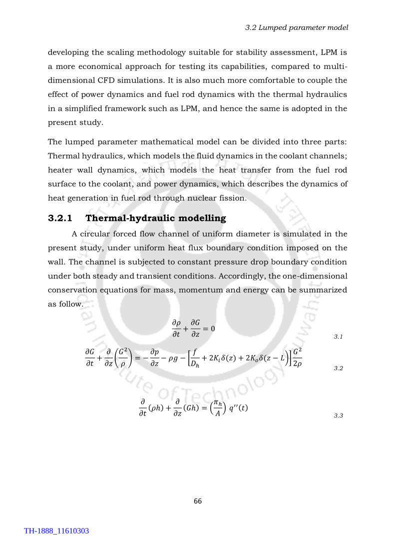
3.2 Lumped parameter model
66
developing the scaling methodology suitable for stability assessment, LPM is
a more economical approach for testing its capabilities, compared to multi-
dimensional CFD simulations. It is also much more comfortable to couple the
effect of power dynamics and fuel rod dynamics with the thermal hydraulics
in a simplified framework such as LPM, and hence the same is adopted in the
present study.
The lumped parameter mathematical model can be divided into three parts:
Thermal hydraulics, which models the fluid dynamics in the coolant channels;
heater wall dynamics, which models the heat transfer from the fuel rod
surface to the coolant, and power dynamics, which describes the dynamics of
heat generation in fuel rod through nuclear fission.
3.2.1 Thermal-hydraulic modelling
A circular forced flow channel of uniform diameter is simulated in the
present study, under uniform heat flux boundary condition imposed on the
wall. The channel is subjected to constant pressure drop boundary condition
under both steady and transient conditions. Accordingly, the one-dimensional
conservation equations for mass, momentum and energy can be summarized
as follow.
𝜕𝜌
𝜕𝑡+
𝜕𝐺
𝜕𝑧= 0
3.1
𝜕𝐺
𝜕𝑡+
𝜕
𝜕𝑧(𝐺2
𝜌) = −
𝜕𝑝
𝜕𝑧− 𝜌𝑔 − [
𝑓
𝐷ℎ+ 2𝐾𝑖𝛿(𝑧) + 2𝐾𝑜𝛿(𝑧 − 𝐿)]
𝐺2
2𝜌
3.2
𝜕
𝜕𝑡(𝜌ℎ) +
𝜕
𝜕𝑧(𝐺ℎ) = (
𝜋ℎ
𝐴) 𝑞′′(𝑡)
3.3
TH-1888_11610303

3.2 Lumped parameter model
67
Heat loss to the surrounding is neglected here. For the sake of generalizations,
governing equations are non-dimensionalized using the following definitions.
𝑧∗ =
𝑧
𝐿𝑐
, 𝑡∗ =𝑡𝐺𝑐
𝜌𝑝𝑐𝐿𝑐
, 𝐺∗ =𝐺
𝐺𝑐
, 𝜌∗ =𝜌
𝜌𝑝𝑐
, 𝑝∗ =(𝑝 − 𝑝𝑟)𝜌𝑝𝑐
𝐺𝑐2
,
𝑇∗ =𝑇 − 𝑇𝑝𝑐
𝑇𝑝𝑐
, ℎ∗ = (ℎ − ℎ𝑝𝑐)𝛽�̅�𝑐
𝐶𝑝.𝑝𝑐
, 𝑁𝐹𝑟 =𝐺𝑐
2
𝜌𝑝𝑐2 𝑔𝐿𝑐
,
𝑁𝑇𝑃𝐶 =𝑞0
′′𝜋ℎ𝐿𝑐
𝐴𝐺𝑐
𝛽𝑝𝑐
𝐶𝑝.𝑝𝑐, 𝑁𝐸𝑢 =
𝑓𝐿𝑐
2𝐷ℎ
3.4
Reference pressure (𝑝𝑟) can be set to any suitable value, as the system thermal
hydraulics is generally quite independent of pressure in the supercritical level.
Hence, the outlet pressure is selected as the reference for the present work.
Subsequently, the non-dimensional forms of governing equations can be
presented as,
𝜕𝜌∗
𝜕𝑡∗+
𝜕𝐺∗
𝜕𝑧∗= 0
3.5
𝜕𝐺∗
𝜕𝑡∗+
𝜕
𝜕𝑧∗(𝐺∗2
𝜌∗) = −
𝜕𝑝∗
𝜕𝑧∗−
𝜌∗
𝑁𝐹𝑟− [𝑁𝐸𝑢 + 𝐾𝑖𝛿
∗(𝑧∗) + 𝐾𝑜𝛿∗(𝑧∗ − 1)]
𝐺∗2
𝜌∗
3.6
𝜕
𝜕𝑡∗(𝜌∗ℎ∗) +
𝜕
𝜕𝑧∗(𝐺∗ℎ∗) = 𝑁𝑇𝑃𝐶 𝑓(𝑡∗)
3.7
Here𝛿, dimensional Dirac delta functions (m-1) at channel inlet and exit
simulate the localized pressure losses at entry and exit respectively. Number
of non-dimensional parameters and dimensionless groups (Eq. 3.4) are
defined to transform the set of dimensional equations into a non-dimensional
one for the sake of generalization.
Choice of the reference pressure (𝑝𝑟) is quite arbitrary and hence the channel
exit pressure is selected as the reference here, so that the pressure drop
across the channel (∆𝑝) can be equated to the inlet value alone in the non-
dimensional scale. The boundary conditions can be specified in terms of two
dimensionless numbers, namely, 𝑁𝑇𝑃𝐶 and 𝑁𝑆𝑃𝐶 (= 𝛽𝑝𝑐(ℎ𝑝𝑐 − ℎ𝑖) 𝐶𝑝.𝑝𝑐⁄ ). While
the former represents system power, the latter is proportional to (ℎ𝑝𝑐 − ℎ𝑖) and
TH-1888_11610303
3.2 Lumped parameter model
68
hence can be taken as a measure of the inlet temperature. While the former
signifies the non-dimensional enthalpy differential between the inlet and the
pseudocritical point, the latter corresponds to the power input to the channel.
They can be viewed to be analogous respectively to the subcooling number
and phase-change number for a boiling channel.
Here the definition of 𝑁𝑇𝑃𝐶 corresponds to some reference power level 𝑞0′′ and
the function 𝑓(𝑡∗) captures the transient variation in the power supply, which
in turn is dependent on the neutronics.
3.2.2 Fuel dynamics
The heat transfer from the fuel rod to the coolant is defined by fuel
dynamics. The internal thermal resistance of the fuel rod is assumed
negligible compared to the external resistance to heat transfer between the
heater and coolant. Hence, the temperature distribution inside the fuel rod is
neglected, and it is considered as a body having a uniform temperature. The
effects of heat conduction through the cladding, gap conductance, and heat
diffusion through the fuel pellet have been neglected for simplicity, as it does
not hamper the overall dynamics of the system (Regis et al., 2000; Yang and
Zavaljevski, 2003). The purpose of ignoring the diffusion through the fuel
element is to reduce the complexity. The primary goal of the analysis is to
simulate the practical conditions simply and to provide the preliminary data
for the more rigors analysis using this model. So that, the model can able to
capture marginal stability boundary quickly and effectively. The fuel element
chosen is Uranium dioxide having a heat capacity of 3.46 MJ/m3K (Zhao et
al., 2006).
Fuel rod dynamics is considered in the present model to study its effect on
the stability of the system. The rate of heat transfer being proportional to the
fuel-to-coolant temperature differential, it becomes imperative to consider
temperature as a function of enthalpy, which has been designated as one of
the primary variables in LPM. A single node for the fuel rod is found, assuming
uniform temperature throughout, in conjunction with the two thermal
TH-1888_11610303

3.2 Lumped parameter model
69
hydraulic nodes. Accordingly, the energy balance for the fuel rod,
characterized by a constant steady-state power (Pss), can be presented as,
𝐶𝑓
𝑑𝑇𝑓
𝑑𝑡= 𝑃𝑠𝑠 − 𝛼1𝐴1(𝑇𝑓 − 𝑇1) − 𝛼2𝐴2(𝑇𝑓 − 𝑇2)
3.8
Here 𝑇𝑗, 𝐴𝑗 and 𝛼𝑗 respectively represents the average temperature, total
peripheral area and convective heat transfer coefficient for the 𝑗th fluid node,
whereas 𝑇𝑓 is the average temperature for the fuel rod. Average coolant
temperature for each node is taken as the mean of the inlet and outlet values
for that particular node. Since enthalpy is selected as the primary variable in
the present analysis, temperature is considered as a piecewise quadratic
polynomial function of enthalpy.
With the incorporation of the lumped fuel rod model, the energy equation for
the 𝑗th coolant node (Eq. (3.8)) needs to be modified as,
𝜕
𝜕𝑡(𝜌ℎ)𝑗 +
𝜕
𝜕𝑧(𝐺ℎ)𝑗 = (
𝜋ℎ
𝐴)𝑛𝑓𝛼𝑗(𝑇𝑓 − 𝑇𝑗)
3.9
where 𝐴 refers to the cross-sectional area of the channel and 𝑛𝑓 is the number
of fuel rods involved. Using the non-dimensional definitions proposed in Eq.
(3.4), dimensionless forms of the above two equations can be given as:
𝜏𝑑𝑇𝑓
∗
𝑑𝑡∗= 1 − 𝐻1𝑧𝑝𝑐
∗ (𝑇𝑓∗ − 𝑇1
∗) − 𝐻2(1 − 𝑧𝑝𝑐∗ )(𝑇𝑓
∗ − 𝑇2∗)
3.10
𝜕
𝜕𝑡∗(𝜌∗ℎ∗)𝑗 +
𝜕
𝜕𝑧(𝐺∗ℎ∗)𝑗 = 𝑁𝑗
′(𝑇𝑓∗ − 𝑇𝑗
∗)
3.11
where, 𝜏 =𝐶𝑓𝐺𝑐𝑇𝑝𝑐
𝜌𝑝𝑐𝐿𝑐𝑃𝑠𝑠 𝐻𝑗 =
𝛼𝑗(𝑛𝑓𝜋ℎ𝐿𝑐)𝑇𝑝𝑐
𝑃𝑠𝑠 𝑁𝑗
′ =𝑃𝑠𝑠𝐻𝑗𝛽𝑝𝑐
𝐴𝐺𝑐𝐶𝑝.𝑝𝑐
3.2.3 Power dynamics
In nuclear reactors, the heat is generated due to fission. The theory
behind this is the Neutron transport theory (Henry, 1975). It is used to explain
the time-dependent behavior of neutron population in the reactor. This theory
TH-1888_11610303

3.2 Lumped parameter model
70
allows for a precise representation of neutron interactions. The resulting
equations are, however, mathematically complex due to their explicit
dependence on neutron energy, the direction of motion, and position, and
time. If equations depend on time then it would easily be handled. Under
certain conditions, it is possible and widely useful to suitably integrate or
average out energy, direction and position variables from the time-dependent
transport theory equations, resulting in a set of ordinary differential equations
with respect to time, in which the delayed neutrons can be retained if desired
(Pandey, 1996).
It is recognized by different researchers that the delayed neutron emitters
have the widely different decay constant and are better represented by six
group of delayed neutron precursors. It is convenient and satisfactory (and
most widely used in lumped parameter models) to treat the delayed neutron
precursors using one precursor group model. This simplifies the equations by
representing all the delayed neutrons as though they had a single mean
lifetime or decay constant. Point reactor kinetics model with one group of
delayed neutrons (Park et al., 1986; Theler and Bonetto, 2010; Pandey and
Singh, 2016; Prasad et al., 2007), is widely used in linear and nonlinear
analysis of nuclear-coupled thermal-hydraulic analysis, and as stated earlier
the main objective of the model is to qualitative study with reasonable
accuracy, hence by using the 6-groupes of delayed neutron. The mathematical
model become more complicated nonlinear equations, which does not gives
more advantage on the qualitative basis. Hence, the choice of one group of
delayed neutron is justified. Finally, the resultant point reactor kinetics
equations are coupled with the suitably reduced-order thermal-hydraulic
model of the reactor core, with appropriate reactivity feedback mechanism, to
yield a lumped parameter model. Point neutron kinetics with a single group
of delayed neutrons is also incorporated in the developed model to embrace
the effect of power dynamics. The constant steady-state power 𝑃𝑠𝑠 mentioned
in the previous discussion is subsequently replaced by a time-varying
TH-1888_11610303

3.2 Lumped parameter model
71
quantity. Transient variation in power and precursor density can be presented
as,
𝑑𝑃
𝑑𝑡=
𝑘 − 𝛽
𝛾𝑃 + 𝜎𝐶
3.12
𝑑𝐶
𝑑𝑡=
𝛽
𝛾𝑃 − 𝜎𝐶
3.13
Setting the steady-state reactivity to zero and neglecting the time-dependence,
the feedback reactivity can be correlated to the fuel rod temperature and
coolant enthalpy as,
𝑘(𝑡) = 𝜇𝑓(𝑇𝑓(𝑡) − 𝑇𝑓,𝑠𝑠) + 𝜇ℎ1(ℎ1(𝑡) − ℎ1,𝑠𝑠) + 𝜇ℎ2(ℎ2(𝑡) − ℎ2,𝑠𝑠) 3.14
where 𝜇𝑓 is the temperature coefficient of reactivity and 𝜇ℎ𝑗 is the enthalpy
coefficient of reactivity for the 𝑗th fluid node. Here the feedback at any time
instant is considered to correspond to the average fuel rod temperature and
average coolant enthalpies at each node at that particular instant. The
variables related to power dynamics can be non-dimensionalized using the
concerned steady-state values as,
𝑃∗ =
𝑃
𝑃𝑠𝑠
, 𝐶∗ =𝐶
𝐶𝑠𝑠
3.15
Consequently, the dimensionless versions of Eq. (3.12) and (3.13) can be
presented as,
𝑑𝑃∗
𝑑𝑡∗=
𝑘 − 𝛽
𝛾𝑃∗ + 𝜎𝐶∗
3.16
𝑑𝐶∗
𝑑𝑡∗=
𝛽
𝛾𝑃∗ − 𝜎𝐶∗
3.17
Variation in the non-dimensional power 𝑃∗ determines the nature of Eq. 3.17,
thereby providing the coupling between the neutronics and thermal hydraulic
components. The reference power can be defined as, 𝑃𝑠𝑠 = 𝑞0′′𝜋ℎ𝐿𝑐. Magnitudes
of the neutronics constants are taken from BWR designs, since all light water
TH-1888_11610303

3.3 Steady-state equations
72
reactors are typically characterized by similar numbers. Values for both the
coefficients are taken from the work of Yang (2010).
3.3 Steady-state equations
The steady equations are obtained by putting the temporal derivatives
zero in Eq. 3.5-3.7, 3.10, 3.16 and Eq. 3.17.
𝜕𝐺∗
𝜕𝑧∗= 0
3.18
𝜕
𝜕𝑧∗(𝐺∗2
𝜌∗) = −
𝜕𝑝∗
𝜕𝑧∗−
𝜌∗
𝑁𝐹𝑟
− [𝑁𝐸𝑢 + 𝐾𝑖𝛿∗(𝑧∗) + 𝐾𝑜𝛿∗(𝑧∗ − 1)]
𝐺∗2
𝜌∗
3.19
𝜕
𝜕𝑧∗(𝐺∗ℎ∗) = 𝑁𝑇𝑃𝐶
3.20
1 − 𝐻1𝑧𝑝𝑐∗ (𝑇𝑓
∗ − 𝑇1∗) − 𝐻2(1 − 𝑧𝑝𝑐
∗ )(𝑇𝑓∗ − 𝑇2
∗) = 0
3.21
𝑘 − 𝛽
𝛾𝑃∗ + 𝜎𝐶∗ = 0
3.22
𝛽
𝛾𝑃∗ − 𝜎𝐶∗ = 0
3.23
Eq. 3.18-3.23, shows the steady state equations of the five state variables
namely, 𝑧𝑝𝑐∗ ℎ𝑜
∗ 𝑇𝑓∗ 𝑃∗ 𝐶∗ . Eq. 3.18 is the equation of mass flux at steady
state. There are two equations (Eq. 3.19-3.20) which captures the
thermohydraulic aspects of the system. Moreover, one equation (Eq. 3.21) is
coming from the fuel dynamics of the system, which gives the steady state
value of average fuel rod temperature, finally the last two equations (Eq. 3.22-
3.23) is provides the information of the power dynamics of the system.
The above equations, in addition to the equation of state, are solved by using
MATLAB ODE function 15s, which is an in-built ordinary differential equation
solver in MATLAB, when all the inlet field variables, i.e., pseudocritical length,
enthalpy, fuel rod temperature, power and precursor density are specified.
The results obtained from the steady state model are used as the initial
condition for the transient simulation.
TH-1888_11610303

3.3 Steady-state equations
73
3.3.1 Comparison of steady state results
The results from LPM are compared with the 1-D models proposed by
Ambrosini and Sharabi (2008). In their model, different inlet and exit orifice
pressure drop coefficients were used to match the steady state axial pressure
distribution obtained by them. The comparison of the steady state result at a
power input of 25 kW/m obtained by LPM with those from the Ambrosini and
Sharabi (2008) model is shown in Figure 3-2 and Figure 3-3. The geometrical
and operating parameters of the problem under consideration are given in
Table 3-2.
Table 3-2: Geometrical and operating parameters of the single channel (Ambrosini and Sharabi, 2008)
Geometrical parameters
Length 4.2672 m
Hydraulic diameter 3.4 mm
Coolant flow area 5.4972 × 10⁻⁵ m2
Operating parameters
Inlet temperature 280◦C
Inlet pressure 25.14 MPa
Exit pressure 25.00 MPa
Based on the above observations, it has been concluded that the LPM steady-
state results are matches well, which is within the acceptable limits.
TH-1888_11610303

3.4 Transient equations
74
Figure 3-2: Comparison of the steady state pressure distribution along the channel for the single channel obtained by LPM with Ambrosini and Sharabi (2008)
Figure 3-3: Comparison of the steady state density distribution along the channel for the single channel obtained by LPM with Ambrosini and Sharabi (2008)
Finally, from these calculations, results in reasonable agreement with the
data reported in the mentioned reference.
3.4 Transient equations
The general transient equations are complicated to solve because of the
coupling between the momentum and energy equations. Due to their
nonlinear nature, It is possible to simplify these equations in two ways; by
25
25.02
25.04
25.06
25.08
25.1
25.12
25.14
25.16
0 1 2 3 4 5
Pre
ssu
re (
MP
a)
z (m)
Ambrosini LPM
0
100
200
300
400
500
600
700
800
0 0.5 1 1.5 2 2.5 3 3.5 4
ρ(k
g/m
3)
z (m)
Ambrosini LPM
TH-1888_11610303

3.4 Transient equations
75
decoupling the momentum and energy equations using an approximate
velocity distribution in the channel, or by transforming the PDEs to ODEs,
which can be solved separately in the time- and space-domain. The latter
approach is the foundation of the method of characteristics. In the channel
integral (CI) method detailed by Todreas and Kazimi (2001), the mass,
momentum and energy equations are integrated over the entire length of the
channel. The present model adopts a two-zone LPM-based approach following
the similar methodology. Two different types of boundary conditions are
studied separately, which are the constant pressure drop and constant mass
flow rate respectively, along with specified coolant inlet temperature.
3.4.1 Pressure drop boundary condition
The non-dimensional governing equations are integrated over the first
and second node respectively. In the first node the mass and energy equations
are integrated separately from inlet until the appearance of the pseudocritical
point, following two ODEs can be obtained.
𝐵2
𝑑𝑧𝑝𝑐∗
𝑑𝑡∗= (𝐺𝑝𝑐
∗ − 𝐺𝑖∗)
3.24
𝐵1
𝑑𝑧𝑝𝑐∗
𝑑𝑡∗= (𝑁𝑇𝑃𝐶𝑧𝑝𝑐
∗ + 𝑁𝑆𝑃𝐶𝐺𝑖∗)
3.25
Where, 𝑁𝑇𝑃𝐶 =𝑞0
′′𝜋ℎ𝐿𝑐
𝐴𝐺𝑐
𝛽𝑝𝑐
𝐶𝑝.𝑝𝑐 𝑎𝑛𝑑 𝑁𝑆𝑃𝐶 = 𝛽𝑝𝑐(ℎ𝑝𝑐 − ℎ𝑖) 𝐶𝑝.𝑝𝑐⁄ . Above two ODEs can be
combined to obtain the following algebraic equation of inlet mass flux.
𝐵3𝐺𝑖∗ = 𝐵1𝐺𝑝𝑐
∗ − 𝑁𝑇𝑃𝐶𝐵2𝑧𝑝𝑐∗
3.26
Again, Integrating the non-dimensional mass and energy conservation
equations over the second node, from the pseudocritical point to the channel
outlet, two ODEs are achieved in terms of ℎ𝑜∗ .
ℎ𝑜∗𝑑ℎ𝑜
∗
𝑑𝑡∗=
(𝐺𝑜∗ − 𝐺𝑝𝑐
∗ ) + (1 − 𝐵4)𝑑𝑧𝑝𝑐
∗
𝑑𝑡∗
(𝐵4 − 𝐵5)(1 − 𝑧𝑝𝑐∗ )
3.27
TH-1888_11610303

3.4 Transient equations
76
ℎ𝑜∗𝑑ℎ𝑜
∗
𝑑𝑡∗=
𝑁𝑇𝑃𝐶(1 − 𝑧𝑝𝑐∗ ) − 𝐺𝑜
∗ℎ𝑜∗ − (1 − 𝐵4)
𝑑𝑧𝑝𝑐∗
𝑑𝑡∗
(𝐵4 − 𝐵5)(1 − 𝑧𝑝𝑐∗ )
3.28
Similar to the first node, the above two ODEs can also be combined in a single
equation as,
𝐺𝑝𝑐
∗ = 𝐺𝑜∗(ℎ𝑜
∗ − 1) − 𝑁𝑇𝑃𝐶(1 − 𝑧𝑝𝑐∗ ) − 2(1 − 𝐵4)
𝑑𝑧𝑝𝑐∗
𝑑𝑡∗
3.29
Finally, the equation for conservation of momentum is integrated separately
over both the zones and added to represent the net pressure drop across the
channel as,
∆𝑝∗ =1
2(𝑑𝐺𝑖
∗
𝑑𝑡∗+
𝑑𝐺𝑜∗
𝑑𝑡∗) + ∆𝑝𝑓
∗ + ∆𝑝𝑔∗ + ∆𝑝𝑎
∗ + ∆𝑝𝐿,𝑖∗ + ∆𝑝𝐿,𝑜
∗ 3.30
where, ∆𝑝𝑓∗ =
𝐺𝑝𝑐∗2𝑁𝐸𝑢
2[1 +
1
2 𝑁𝑆𝑃𝐶
ln(1 + 2 𝑁𝑆𝑃𝐶)] 𝑧𝑝𝑐∗ +
𝐺𝑜∗2𝑁𝐸𝑢
2(2 + ℎ𝑜
∗)(1 − 𝑧𝑝𝑐∗ )
∆𝑝𝑔∗ = [(1 − 𝐵2)𝑧𝑝𝑐
∗ + 𝐵4(1 − 𝑧𝑝𝑐∗ )] 𝑁𝐹𝑟
−1
∆𝑝𝑎∗ = 𝐺𝑜
∗2(1 + ℎ𝑜∗) −
𝐺𝑖∗2
𝜌𝑖∗ ∆𝑝𝐿,𝑖
∗ =𝐾𝑖
2𝜌𝑖∗ 𝐺𝑖
∗2 ∆𝑝𝐿,𝑜∗ =
𝐾𝑜
2𝐺𝑜
∗2(1 + ℎ𝑜∗ )
As the system under consideration is subjected to the specified pressure drop
boundary condition, Eq. (3.21) is coupled with the differentiated form of Eq.
(3.22) to provide an equation of outlet mass flux as
𝑑𝐺𝑜∗
𝑑𝑡∗= [2∆𝑝𝐼𝑛𝑒𝑟𝑡𝑖𝑎𝑙
∗ − {𝐺𝑖∗ − 𝐺𝑜
∗ − 𝑁𝑇𝑃𝐶
𝐵2
𝐵3𝑧𝑝𝑐
∗ }𝑑𝑧𝑝𝑐
∗
𝑑𝑡∗
− {1 +𝐵1
𝐵3
𝑧𝑝𝑐∗ }
𝑑𝐺𝑝𝑐∗
𝑑𝑡∗] (1 − 𝑧𝑝𝑐
∗ )−1
3.31
where, 𝐵1 =
ln(1 + 𝑁𝑆𝑃𝐶)
𝑁𝑆𝑃𝐶− (1
+ 𝑁𝑆𝑃𝐶)
𝐵2 =ln(1 + 𝑁𝑆𝑃𝐶)
𝑁𝑆𝑃𝐶− 1 𝐵3 = 𝐵1 + 𝐵2𝑁𝑆𝑃𝐶
TH-1888_11610303

3.4 Transient equations
77
𝐵4 =1
ℎ𝑜∗ln (1 + ℎ𝑜
∗) 𝐵5 =1
1 + ℎ𝑜∗
Therefore, the initial system of PDEs is converted to a set of algebraic
equations and ODEs, with dimensionless time (𝑡∗) as the sole independent
variable. That eliminates the complexity associated with solving a system of
PDEs and eradicates the huge computational resource requirement for finite
difference simulation. In order to capture the sharp variation in
thermophysical properties of supercritical water around the pseudocritical
point, the equation of state is replaced by fitting a separate rectangular
hyperbola for each of the zones (Figure 3-4) given as (Pandey and Kumar,
2007),
𝜌∗ =
1 − 2ℎ∗
1 − ℎ∗ 𝑓𝑜𝑟 − 1.58 ≤ ℎ∗ ≤ 0
𝜌∗ =1
1 + ℎ∗ 𝑓𝑜𝑟 0 ≤ ℎ∗ ≤ 1.74
3.32
Figure 3-4: Polynomial fitting of IAPWS data for water at 25 MPa
3.4.2 Mass flow rate boundary condition
For considering mass flow rate boundary condition, the same procedure
is applied as mentioned in Section 3.3.1, integrating the dimensionless
0.0
0.5
1.0
1.5
2.0
-2 -1 0 1 2
ρ*
h*
1st zone
2nd zone
Water
TH-1888_11610303

3.5 RELAP model
78
governing equations for mass and energy over the first node, the following two
ODEs is obtained.
𝐵2
𝑑𝑧𝑝𝑐∗
𝑑𝑡∗= (𝐺𝑝𝑐
∗ − 𝐺𝑖∗)
3.33
𝐵1
𝑑𝑧𝑝𝑐∗
𝑑𝑡∗= (𝑁𝑇𝑃𝐶𝑧𝑝𝑐
∗ + 𝑁𝑆𝑃𝐶𝐺𝑖∗)
3.34
where, 𝑁𝑆𝑃𝐶 =𝛽�̅�𝑐(ℎ𝑝𝑐 − ℎ𝑖)
𝐶𝑝,𝑝𝑐
The above two ODEs can be combined to obtain the following algebraic
equation of inlet mass flux.
𝐵1𝐺𝑝𝑐∗ = 𝐵3𝐺𝑖
∗ + 𝑁𝑇𝑃𝐶𝐵2𝑧𝑝𝑐∗
3.35
Integrating the conservation equations over the second node, from the
pseudocritical point to the channel outlet, two ODEs of ℎ𝑜∗ is obtained. After
combining the ODEs of ℎ𝑜∗ equations, an algebraic equation of 𝐺𝑜
∗, is obtained.
𝐺𝑜
∗(ℎ𝑜∗ − 1) = 𝐺𝑝𝑐
∗ − 𝑁𝑇𝑃𝐶(1 − 𝑧𝑝𝑐∗ ) − 2(1 − 𝐵4)
𝑑𝑧𝑝𝑐∗
𝑑𝑡∗
3.36
The equation for conservation of momentum is not taken into considerations
as the mass flow rate boundary condition is applied here.
where, 𝐵1 =
ln(1 + 𝑁𝑆𝑃𝐶)
𝑁𝑆𝑃𝐶− (1
+ 𝑁𝑆𝑃𝐶)
𝐵2 =ln(1 + 𝑁𝑆𝑃𝐶)
𝑁𝑆𝑃𝐶
− 1 𝐵3 = 𝐵1 + 𝐵2𝑁𝑆𝑃𝐶
𝐵4 =1
ℎ𝑜∗ln (1 + ℎ𝑜
∗) 𝐵5 =1
1 + ℎ𝑜∗
3.5 RELAP model
RELAP5 is a highly generic code that, in addition to calculating the
behaviour of a reactor coolant system during transients, can be used for
simulation of a wide variety of hydraulic and thermal transients in both
nuclear and non-nuclear systems. It is a sophisticated time-domain code
based on two-fluid formulations, capable of simulating the flow at
TH-1888_11610303

3.5 RELAP model
79
supercritical pressures (Fu et al., 2012; Debrah et al., 2013). Present layout
is visualized in RELAP5/MOD4.0 code as a single pipe, connected with inlet
and outlet plenum (Figure 3 3). The single channel is modelled as a pipe
component, containing 30 volumes, connected with junctions at the two ends.
These junctions are further combined with time-dependent volume
components to model the plenum. The heat supply to the active core is shaped
using heat structures, which is subsequently divided into volumes similar to
the active core and with constant power option. The heat structure is modelled
as a material having high thermal conductivity and low heat capacity, to avoid
distortions in the imposed thermal flux condition, and eliminating the effect
of fuel dynamics. Accordingly, RELAP is employed to validate the thermal-
hydraulic part of the present model solely.
To ascertain the stability behaviour of the RELAP model, simulations are
initially performed at some guessed power level, often guided by the
observations from the indigenous linear stability analysis. Generally, lower
values of power are attempted with, to ensure a stable response, which can
be concluded by following the resultant temporal variation in system
variables. Subsequently, the power is gradually increased until the
attainment of the marginally stable condition, signified by constant-amplitude
fluctuations of the state variables. With the small rise in power level, the code
returns diverging oscillations, indicating the unstable situation. Such hit-
and-trial approach requires several simulations to identify the stability
threshold and consequently to generate the stability map.
TH-1888_11610303

3.5 RELAP model
80
Figure 3-5: Nodalization diagram
3.5.1 Nodal sensitivity test
The influence of nodalization on the system stability has been
investigated performing a sensitivity analysis on the RELAP model. The
observations are made based on three different RELAP model having 10, 30
and 50 nodes respectively. Based on these observations, a stability map,
Figure 3-6 has been plotted which shows the good agreement between models.
Based on this study, the second model, which have 30 nodes, is selected for
analysis in the present work.
TH-1888_11610303

3.5 RELAP model
81
Figure 3-6: Nodal sensitivity for three different volumes
3.5.2 Comparison of LPM and RELAP5
Comparison of numerical results in terms of stability map is
preliminary done with the RELAP5. This will give the initial idea about the
dynamics of system. Also, RELAP is used by several researchers (Ambrosini
and Sharabi, 2008; Colombo et al., 2012) for the validation of their code,
hence it is useful as a first-hand toll for the beginning. The comparison with
RELAP shows good consistency of the LPM model. Therefore, all the
simulations are completed using LPM. RELAP5 transient simulations are
carried out with various operating conditions, such as at 25 MPa pressure for
finding the threshold of the stability. Here the single channel is modelled as a
pipe component, with 30 volumes, connected with junctions at the two ends.
These junctions are further connected with time dependent volume
components to simulate the plena. The heat supply to the active core is
simulated through heat structures, which is divided into the same number of
volumes, as the active core. Corresponding nodalization diagram is shown in
Figure 3-5.
Maintaining identical magnitudes of the initial and boundary conditions,
simulations are performed with various sets of operating. Stability maps
obtained with all the three tools employed here, namely linear stability
analysis, transient simulation with LPM and RELAP5, are compared in Figure
1.5
1.9
2.3
2.7
3.1
6 6.5 7 7.5 8 8.5 9
Nsp
c
Ntpc
10 Volume
30 Volume
50 Volume
Stable
Unstable
TH-1888_11610303
3.5 RELAP model
82
3.7. All of them exhibit qualitatively similar profiles, as a progressive increase
in heating power under a constant pressure drop across the channel
eventually leads to instability. However, the LPM is found to yield a
conservative estimate, with stability threshold corresponding to lower power
values for any given inlet conditions. Prediction from the linear stability
analysis matches exactly with transient simulations and that is only logical,
as they employ the same set of mathematical equations. The disparity with
RELAP5 can be ascribed to the lumped nature of fluid properties over both
the zones. RELAP5 discretizes the channel in larger number of nodes, 30 in
present model, compared to just two in LPM and hence in a better position to
handle the rapid variation in properties around the pseudocritical point,
although at the expense of significantly more computational resource
obligation and substantial expertise requirement in handling the code.
The stability of the system is inferred from the nature of time evolutions of
different variables like geometrical parameter, operating parameter and mass
flow rate. The non-dimensional stability maps generated using LPM and
RELAP5 are shown in Figure 3-7. It can be easily observed that the qualitative
behaviour of both the maps is similar. The Stable region of the LPM is a subset
of the stable region of RELAP5. Thus, despite many simplifying assumptions,
the lumped parameter model is conservative
TH-1888_11610303

3.6 Validation of LPM with the experimental result
83
Figure 3-7: Comparisons of LPM with RELAP .
3.6 Validation of LPM with the experimental result
Figure 3-8: Validation of LPM with experimental data (Xi et al. (2014))
Limited number of papers available, which provide the experimental
results based on the single channel, forced flow instability of SCWR. There
are good numbers of paper available which uses RELAP5 for the validation
purpose of their numerical works (Colombo et al., 2012; Kozmenkov et al.,
2012; Mousavian et al., 2004; Papini et al., 2012).
1.5
1.7
1.9
2.1
2.3
2.5
2.7
2.9
3.1
6 6.5 7 7.5 8 8.5 9 9.5
Nsp
c
Ntpc Dynamic simulation at 25MPa Linear Stability at 25MPa RELAP
Stable
Unstable
1.5
2
2.5
3.3 3.5 3.7 3.9
NS
PC
NTPC
Numerical Experimental (Xi, 2014)
Stable
Unstable
TH-1888_11610303

3.6 Validation of LPM with the experimental result
84
Zhao et al. (2005) has used experimental (Khabensky and Gerliga, 1995) data
for the validation of his single channel three zone supercritical LPM model.
Due to the limited information available such as, no information regarding
the inlet and outlet restrictions and many more important details of the
experiment (Yu, 1965), and as this was the only set of relevant data they could
find on the stability boundary at supercritical pressure, they were bound to
use the same. Therfore, the predicted stability boundary agreed with the
experimental stability boundary within ±30%.
In the flow instability experiment between two parallel channels with
supercritical water, which was carried out by Xiong et al. (2012), according to
his paper, due to the inadequacy of test section in the experiment, not so
many results were obtained. The tube which were used for the experiment,
INCONEL 625 pipes with inner diameter of 6 mm and outer diameter of 11
mm (Xiong et al., 2012), in which wall thickness of two tubes is just 2.5 mm,
with which not sufficient experiment results could be obtained due to the
limitation of pipe strength under high outlet temperature and pressure.
According to Xi et al., (2014a) the codes, which were used for comparing with
the experiment, could not predict the oscillation period well, there was a
considerable difference between numerical simulation and experiment.
Keeping these points into consideration the experimental validation has been
done using Xi et al., (2014a) instead of Xiong et al. (2012) and others. Again,
due to the scarcity of relevant articles on experimental study, few of the recent
numerical works have also been compared and validated there numerical
works (Li et al., 2018; Shitsi et al., 2018; Zhang et al., 2015) using the
previous paper.
Figure 3-8 shows the comparison between the numerical and experimental
data on the nondimensional plan; stability map having two axes as NTPC and
NSPC. The stability map shows the similar trend, indicate that the numerical
code is capable of predicting stability boundaries, as the relative errors are
within ±7% range, which is the convincing range for validation.
TH-1888_11610303

3.6 Validation of LPM with the experimental result
85
Table 3-3: Comparison of experimental and predicted stability boundary
Pressur
e (MPa)
Inlet
Enthalp
y (kJ/kg)
Power/mas
s flow rate
(kW/(kg/s))
Experimenta
l NTPC
Numerica
l NTPC
Relative
Error
|𝑁𝑇𝑃𝐶,𝑒𝑥−𝑁𝑇𝑃𝐶,𝑛𝑢
𝑁𝑇𝑃𝐶,𝑒𝑥|
23 795.63 2270 3.86 3.73 3.36 %
23 905.07 2230 3.79 3.61 4.74 %
23 972.02 2200 3.74 3.51 6.15 %
23 1040.2 2100 3.58 3.45 3.63 %
23 1133.4 2070 3.52 3.39 3.70 %
It is seen from the
Table 3-3, that most of the data points are within ±7% relative error range.
The comparisons of numerical and experimental NTPC shown in Figure 3-9
along with a linear trend line fit.
Figure 3-9: Comparison of experimental and numerical NTPC
This section mainly added to the comparison of numerical results with the
experiment (Xi et al., 2014b). The extractions of experimental data are based
on the paper. Various system parameters including the system pressure, inlet
temperature and total flow rate are tried to be set the same with the
3.3
3.4
3.5
3.6
3.7
3.8
3.5 3.6 3.7 3.8 3.9
Nu
me
ric
al N
TP
C
Experimental NTPC
TH-1888_11610303

3.6 Validation of LPM with the experimental result
86
experiments, to get MSB points obtained as the experiments shows. Then
after changing the system power, further stability analysis has been
performed. To illustrate the comparison in one two-dimensional plane, the
system parameters are interpreted into dimensionless numbers NSPC and NTPC.
The results show a close match with Xi et al. (2014b) that of and the
qualitative behaviour is also similar. It is observed that the plot shows small
discrepancies between the numerical and the experimental result. The
inconsistencies are due to the approximation in the equation of states and a
few other assumptions which have been essential for a simpler model, also
the primary objective of the current work. These discrepancies can be
minimized by the use of better approximations. The reason behind assuming
approximation is that in the present work, the emphasis is given on the
qualitative behaviour of the fixed points. It can be noted that the more
accurate model may be available and provide quite a good match with the
experimental data would be possible, but that can be computationally
expensive. The choice of the model used in the current work is based on its
simplicity and reasonably accurate solutions. The simplicity of the model
allows one to use this reduced order model (ROM) for more complicated, non-
linear stability analysis.
The powers corresponding to MSB in calculations are all lower than those in
experiments. This might be a good indication as the model once again proves
itself as more conservative. The same thing happens during the comparison
of the present model with RELAP (section 3.5.2). In case of RELAP and the
current model, the trends are matching but with experimental validation of
the model, the usual trend is missing. The reason is that RELAP is a transient
code, which uses certain assumptions to solve the given sets of governing
equations, but the actual experimental data could match within the specific
ranges. Moreover, the tread may or may not be matches due to sever
assumptions in the model.
Moreover, the less power corresponding to MSB as compared to the
experimental result might be due to the several assumptions and equations
TH-1888_11610303

3.7 Stability analysis
87
of state in the model. There are various other fundamental differences
between the two; hence the comparisons will not be the same. Few significant
differences are, in the experimental work shows only thermohydraulic results
while the addition of neutronics makes system unpredictable, so from thermal
hydraulics, the prediction of system stability is not fair. Another difference is
that an experiment performed using the parallel channel, which shows some
different dynamics as compared to the current single channel system.
As mention earlier in this section, due to several limitations and a very few
numbers of articles available on experimental results, the need for more depth
study is very much required for the validation of numerical results.
Overall, the purpose of the proposed model is to give the preliminary
qualitative idea of the system behaviour by the simplified model, not the
quantitively. For the latter part, the more rigorous study needs to be
performed by other researchers.
3.7 Stability analysis
The term stability is generally associated with the temporal response of
a dynamical system following an internal or external disturbance during its
operation. There are in fact many different definitions of stability, among
which the following are the most frequently encountered: stability according
to Poisson, stability according to Lyapunov, and asymptotic stability.
Depending on the temporal dynamics of the perturbation, the distinction of
stability is done according to Lyapunov and asymptotic stability. Lyapunov
stability is, if all trajectory that starts sufficiently close to fixed point remains
close to it for all time. It is a very mild requirement on equilibrium points. In
particular, it does not require that trajectories starting close to the origin tend
to the origin asymptotically. Also, stability is defined at a time instant t0
(Anishchenko et al., 2014).
3.7.1 Linear stability analysis
Linear stability analysis is typically the first step in the analysis of a
nonlinear system and is widely used to determine the onset of instabilities
TH-1888_11610303

3.7 Stability analysis
88
and system dynamic behaviour under small perturbations around a steady
state (Appendix-A). This involves linearizing the nonlinear system around the
steady state or equilibrium solution of interest and studying the characteristic
roots of the linearized system.
SCWR being a complex nonlinear system, a rigorous stability analysis is
possible only with some simplifying assumptions. That makes the use of a
linearized model in time domain a necessity, particularly when identification
of the stability boundary is of principal interest. Linear stability analysis is
typically performed by linearizing the nonlinear equations around an
equilibrium solution of interest and studying the characteristic roots of the
linearized system. Dropping the nonlinear terms, a single vector equation of
the following form can be obtained as,
Here 𝐗 = [𝑧𝑝𝑐∗ ℎ𝑜
∗ 𝑇𝑓∗ 𝑃∗ 𝐶∗ ]
𝑇 represents small perturbation around the
steady state𝐗𝟎. The nature of the eigenvalues of the matrix [𝐴] determine the
stability of the solution, as the presence of even a single root on the right-half
plane of the state-space plot indicates an unstable system. In addition to this,
the lumped parameter model (system of nonlinear ordinary differential
equations) is linearized about its steady-state point and the eigenvalues of the
matrix [A] are evaluated. The components of [𝐴] can be obtained from the
lumped parameter equations, leading to stability characterization for any
given set of boundary conditions (Appendix-A).
For performing the stability analysis, the governing equations resulting from
the lumped parameter model are linearized about the steady state. The [𝐴]
resulting from the linearized model is formed and the eigenvalues of this are
evaluated at steady state. If the real parts of all the eigenvalues are negative,
then the system is stable at that operating point. If any of the eigenvalues has
a positive real part, then the system is unstable at that point. The stability
boundary thus formed is the locus of points in the parameter plane for which
the least stable eigenvalue lies on the imaginary axis. It is known from the
Hopf bifurcation theory that the system can have oscillations if the
TH-1888_11610303

3.7 Stability analysis
89
eigenvalues have a complex crossing. It is possible for the system to have
different dynamic behaviour. In one case, if a pair of complex conjugate
eigenvalues crosses the imaginary axis, then the system can have periodic
oscillations. Such oscillations are known as stable limit cycles and the
bifurcation is known as supercritical Hopf bifurcation. In the other case, the
system can have oscillations in the stable region that get decayed for low
perturbations but are amplified for large perturbations. This indicates the
presence of an unstable limit cycle and such a bifurcation is called a sub
critical Hopf bifurcation. This is dangerous from practical point of view, since
the system will have diverging oscillations even though it is designed to
operate in a stable region. The dynamic behavior of the state variables is
obtained by integrating the governing equations in time domain.
3.7.2 Non-linear stability analysis
Linear stability analysis, however, fails to predict certain characteristics
of nonlinear systems, such as the magnitude and frequency of possible limit
cycle oscillations when the system is away from the marginal stability
boundary in the parameter space. That can be ascertained through the
dynamical simulation of the exact nonlinear equations in the time domain by
perturbing any of the variables around a fixed point and subsequently
observing the nature of temporal variations. Dynamics of the perturbed
system may depend on the amplitude of imposed perturbation and several
classes of periodic solutions are possible, (Lahey, 1986) for a boiling channel,
which may happen in SCWR.
The linearly stable region continues to remain stable for small perturbations
around the equilibrium in the presence of nonlinearities. However, the
magnitude of these allowable perturbations depends on the nature of the
bifurcation. For the case of a supercritical Hopf bifurcation, the equilibrium
is globally stable in the linear stability regime and hence the stability of the
solution is insensitive to the magnitude of the perturbation. In contrast, there
are unstable limit cycles around the linearly stable equilibrium for a
subcritical Hopf bifurcation and therefore the equilibrium is stable only to
TH-1888_11610303

3.7 Stability analysis
90
perturbations smaller in magnitude than the amplitude of the unstable limit
cycles. Larger perturbations tend to grow to large magnitudes even in the
linearly stable regime. Therefore, a nonlinear analysis of the problem is
required to ascertain the nature of the Hopf bifurcation. In addition, this
analysis helps us in obtaining the amplitude of the limit cycles emanating
from the Hopf point. This information is especially useful when the nature of
the bifurcation is subcritical as it gives a rough estimate of the magnitude of
perturbations for which the linearly stable equilibrium is nonlinearly stable
as well (Lahey, 1986; Pandey and Singh, 2016; Wahi and Kumawat, 2011).
TH-1888_11610303

3.7 Stability analysis
91
TH-1888_11610303

4.1 Introduction
92
SCALING METHODOLOGY FOR
STABILITY APPRAISAL
4.1 Introduction
Considering the extreme operating conditions associated with the
SCWR and possible consequences of any unforeseen event, it is essential to
investigate all possible aspects of such a system at the laboratory scale, prior
to its commercialization. Accordingly, researchers have shown general
interest towards both the heat transfer and stability behaviour of supercritical
flow systems since the inception of the present millennium. While the current
trend of research is inclined towards numerical and computational (Cheng
and Schulenberg, 2001) analyses, the role of experiments can never be
undermined, particularly in the context of understanding new phenomena
and exploring newer physics. Unfortunately, the associated volume of
experimental literature is rather limited. The review work of Cheng and
Schulenberg (2001) emphasizes on the scarcity of reliable experimental data
in the typical parameter ranges for SCWR, which consequently presents a
huge hurdle in accurate description and prediction of SCWR thermal
hydraulics. That highlights the need of developing experimental facilities and
subsequently necessitates phenomenological scaling, as it is impracticable to
replicate the SCWR condition at lab-scale. Therefore, several attempts
towards scaling of supercritical flow systems are available in open literature.
Considering the similarities between the boiling channels of BWR and heated
supercritical channels, scaling principles are developed following similar
approaches. (Marcel et al., 2009) developed scaling procedure to use a mixture
of R-125 and R-32. With a system pressure of 6.2 MPa, it showed excellent
similarities with SCW at 25 MPa. This mixture, however, has severe
restrictions in terms of flammability limit and chemical stability and requires
accurate monitoring of the mixture composition. Furthermore, they applied
the same scaling rule to both the radial and axial directions, leading to rather
TH-1888_11610303

4.2 Fluid-to-fluid scaling methodology
93
small radial dimension of the experimental facility, and hence resulting in
undesirably large frictional pressure drop. Rhode et al. (2011) proposed an
improved scaling procedure mainly for natural circulation systems based on
R-23 as the model fluid. System pressure, power and temperature levels were
significantly reduced, while preserving the dynamics of the system. Practical
issues, such as the onset of heat transfer deterioration, was also touched
upon in their work. They, however, introduced two multiplication factors for
scaling for the flow rate and friction factor respectively, which require
experiment-based empirical relations, and hence are not universal.
As none of the above-mentioned model fluids properly justifies the stability
analysis due the property and some physical constrains. Therefore, the
primary objectives of the study are to identify a less restrictive model fluid as
compared to the other model fluids, which can properly mimic the SCW under
the relevant scaled condition of an SCWR, and to define the scaling rules in a
generalized way, to preserve the phenomenological physics. Focus is kept on
uncoupling the radial scaling from the axial one, as only then a practicable
combination of system dimensions can be proposed. US reference design of
SCWR is considered as the prototype. Accordingly, the scaled dimensions of
the lab-scale facility and corresponding operational settings in terms of power,
flow rate and inlet temperature are proposed. The advantages of the proposed
methodology over the existing ones have also been stressed upon, along with
a discussion on the role of involved dimensionless groups.
4.2 Fluid-to-fluid scaling methodology
4.2.1 Conservation equations
The most important requirement of the fluid-to-fluid scaling is to
determine the correspondence between the test facilities based on the model
fluid to the prototypical parameter range. The general objective invariably is
to develop a laboratory-scale test facility, which should behave identically to
the prototype in terms of the phenomenon under consideration, and thereby
easy extrapolation of the observations to the prototype-scale. Hence both the
TH-1888_11610303

4.2 Fluid-to-fluid scaling methodology
94
model and prototype must be bound by the same set of conservation
equations and maintain identical values of the characterizing dimensionless
groups. Focus of the present study being the scaling of SCWR core to foretell
the stability behaviour, a single heated channel of constant flow area is
selected, with upward flow and uniform heat flux distribution (Figure 3-1).
Corresponding 1-D equations for conservation of mass, momentum and
energy, which is given in equations (3.1-3.3). Applying the above definitions,
which gives the modified conservation equations (3.5-3.7). It is interesting to
note that the absolute pressure can be freely chosen, since it is not a part of
the balance equations, and hence system pressure is not expected to have
any role on the scaling. A constant pressure drop boundary condition is
employed for simulations with ∆𝑝 = 0.15 MPa.
4.2.2 Scaling principles
As stated above, the scaling objective can be achieved by equating the
characterizing dimensionless groups between the model and prototype. Other
geometric and operating parameters need to be estimated based on the
selection of the scaling fluid. Accordingly, the following factors are considered
to proceed with the scaling.
(a) Nature of non-dimensional property variation of the prototype and model
fluids needs to be identical over the entire range of operating parameters.
(b) From the conservation equations and associated boundary conditions,
several dimensionless groups can be identified including 𝑁𝑇𝑃𝐶, 𝑁𝑆𝑃𝐶, 𝑁𝐹𝑟 and
𝑁𝐸𝑢, which dominate the thermalhydraulic behavior and hence is expected to
govern the stability. Their equality needs to be considered.
(c) There is a total of six parameters required to be scaled. Four of them can
be adjusted independently during the design stage or experimental runs,
namely, the tube diameter, length of heated channel, inlet temperature and
heat flux. Inlet mass flux and pressure drop across the channel are coupled
to each other and one of them can be derived from the imposed boundary
TH-1888_11610303

4.3 Selection of fluids
95
condition. As the present system is subjected to a constant pressure drop
boundary condition, mass flux is a dependent variable here.
(d) Considering the drastic variation of all thermophysical properties of the
supercritical fluid around the pseudocritical point, the same is selected as the
reference point.
4.3 Selection of fluids
Considering the extreme operating conditions associated with SCWR,
the focus of scaling fluid selection is on reducing the power, pressure and
temperature levels of operation. As water experiences drastic variation in all
thermophysical properties around the pseudocritical point, substantial
change in density can be observed across the SCWR core, as SCW is heated
from 280 to 530 °C. Since the scaling fluid must behave similarly over the
entire operational range, selection of model fluid and its operating pressure is
not straight-forward. To be more precise, the equation-of-state for the model
fluid at the selected pressure level must resemble the same for the prototype
fluid on the non-dimensional plane. An extensive comparative analysis is
carried out as a part of the present study using REFPROP v9.1 as the
database for thermophysical properties. As is shown in Figure 4-1, R134a at
a pressure level of 6.2 MPa and CO2 at 8 MPa can simulate water at 25 MPa
with reasonable accuracy.
Figure 4-1: Non-dimensional property variation for three fluids at equivalent pressure levels
0.0
0.5
1.0
1.5
2.0
2.5
3.0
-2.0 -1.5 -1.0 -0.5 0.0 0.5 1.0 1.5 2.0
No
n-d
ime
nsio
na
l de
nsit
y
Non-dimensional enthalpy
Water @ 25.0 MPa
R-134a @ 6.2 MPa
CO2 @ 8.0 MPa
TH-1888_11610303

4.3 Selection of fluids
96
4.3.1 Scaling rules
While the operating pressure level for the model fluid can be selected
by comparing the equation-of-state on 𝜌∗ − ℎ∗ plane, scaling rules need to be
devised to identify other geometric and operating variables. That can be
achieved by equating the dimensionless groups identified earlier.
4.3.2 Pressure
The role of pressure on system characterization is only through the
similarity of the prototypical and model fluids on the 𝜌∗ − ℎ∗ plane and hence
choice of a scale for pressure is quite independent. Accordingly, the scaling
rule for pressure is defined as,
𝑋𝑝 =𝑝𝑚
𝑝𝑝
4.1
4.3.3 Length of the channel
The selected geometry being vertical, the length of the channel is related
to the gravitational forces acting on the system and hence the same has been
scaled by equating the Froude number between the model and prototype.
𝑁𝐹𝑟,𝑚 =
𝐺𝑐2
𝜌𝑝𝑐𝑔𝐿𝑐|𝑚
=𝐺𝑐
2
𝜌𝑝𝑐𝑔𝐿𝑐|𝑝
= 𝑁𝐹𝑟,𝑝 ⇒ 𝑋𝐿 =𝐿𝑐,𝑚
𝐿𝑐,𝑝= [
𝑋𝐺
𝑋𝜌]
2
4.2
Here the density ratio corresponding to the pseudocritical value is defined as,
𝑋𝜌 = 𝜌𝑝𝑐,𝑚 𝜌𝑝𝑐,𝑝⁄ .
4.3.4 Mass flux
The objective of mass flux scaling is to ensure similar nature of heat
transfer behaviour during normal heat transfer process. Present system being
subjected to pressure drop boundary condition and mass flow rate being
directly affected by the same, mass flux is scaled here using the non-
dimensional pressure drop across the channel. It must be the same between
model and prototype and hence,
TH-1888_11610303

4.3 Selection of fluids
97
𝑝𝑚
∗ =∆𝑝 𝜌𝑝𝑐
𝐺𝑐2
|𝑚
=∆𝑝 𝜌𝑝𝑐
𝐺𝑐2
|𝑝
= 𝑝𝑝∗ ⇒ 𝑋𝐺 =
𝐺𝑐,𝑚
𝐺𝑐,𝑝= [𝑋𝑝 𝑋𝜌]
0.5 4.3
4.3.5 Hydraulic diameter
In an effort to differentiate axial and radial scaling, hydraulic diameter
is scaled using the Euler number, as it is responsible for the scaling of
dynamic behaviour of the flow system. Considering identical Euler number
and friction factor between the model and prototype,
𝑁𝐸𝑢,𝑚 =
𝑓𝐿𝑐
𝐷ℎ|𝑚
=𝑓𝐿𝑐
𝐷ℎ|𝑝
= 𝑁𝐸𝑢,𝑝 ⇒ 𝑋𝐷 =𝐷ℎ,𝑚
𝐷ℎ,𝑝= 𝑋𝐿 4.4
4.3.6 Power and inlet temperature
Channel power is scaled in terms of 𝑁𝑇𝑃𝐶 as,
𝑁𝑇𝑃𝐶,𝑚 =
𝑞0′′𝜋ℎ𝐿𝑐𝛽𝑝𝑐
𝐴𝐺𝑐𝐶𝑝.𝑝𝑐
|𝑚
=𝑞0
′′𝜋ℎ𝐿𝑐𝛽𝑝𝑐
𝐴𝐺𝑐𝐶𝑝.𝑝𝑐
|𝑝
= 𝑁𝑇𝑃𝐶,𝑝 ⇒ 𝑋𝑄 =𝑋𝐺𝑋𝐴
𝑋𝐷𝑋𝐿
𝛽𝑝𝑐,𝑝𝐶𝑝.𝑝𝑐,𝑚
𝛽𝑝𝑐,𝑚𝐶𝑝.𝑝𝑐,𝑝
4.5
Similarly 𝑁𝑆𝑃𝐶 can be equated to scale the inlet temperature as,
𝑁𝑆𝑃𝐶,𝑚 =
𝛽𝑝𝑐(ℎ𝑝𝑐 − ℎ𝑖)
𝐶𝑝.𝑝𝑐
|𝑚
=𝛽𝑝𝑐(ℎ𝑝𝑐 − ℎ𝑖)
𝐶𝑝.𝑝𝑐
|𝑝
= 𝑁𝑆𝑃𝐶,𝑝 ⇒ 𝑋ℎ
=(ℎ𝑝𝑐 − ℎ𝑖)|𝑚(ℎ𝑝𝑐 − ℎ𝑖)|𝑝
=𝑋𝐶𝑝,𝑝𝑐
𝑋𝛽𝑝𝑐
4.6
The above similarity can be used to predict the ℎ𝑖𝑛 for the model fluid, which
can further be combined with model pressure to get 𝑇𝑖𝑛.
Fuel rod dynamics is considered in the present model to study its effect on
the stability of the system. The energy balance for the fuel rod, characterized
by a constant steady-state power (𝑃𝑠𝑠), can be presented in equation (3.8). With
the incorporation of the lumped fuel rod model, the energy equation for the
𝑗th coolant node (Eq. (3.3)) needs to be modified as equation (3.9), where 𝐴
refers to the cross-sectional area of the channel and 𝑛𝑓 is the number of fuel
rods involved. Using the non-dimensional definitions proposed in Eq. (3.4),
dimensionless forms of the above two equations (3.10-3.11)
TH-1888_11610303

4.4 Results and discussion
98
Point neutron kinetics with a single group of delayed neutrons is also
incorporated in the developed model to embrace the effect of power dynamics.
Transient variation in power and precursor density can be presented as
equation (3.12-3.13), setting the steady-state reactivity to zero and neglecting
the time-dependence, the feedback reactivity can be correlated to the fuel rod
temperature and coolant enthalpy as equation (3.14). The variables related to
power dynamics can be non-dimensionalized using the concerned steady-
state values as equation (3.15), Consequently the dimensionless versions of
equation (3.16-3.17) can be presented as, magnitudes of the neutronics
constants are taken from BWR designs, since all light water reactors are
typically characterized by similar numbers.
4.4 Results and discussion
Linear stability analysis is used as the tool for appraisal of stability
threshold, which can typically be viewed as the first step in analysing a
nonlinear system and is widely used to determine the onset of instabilities
and system dynamic behaviour under small perturbations around a steady-
state. This involves linearizing the nonlinear system around the steady-state
or equilibrium solution of interest and studying the characteristic roots of the
linearized systemA detailed methodology of stability analysis is discussed in
Nayfeh and Balachandran (1992). Here the eigenvalues of the Jacobian matrix
are calculated for a given set of parameters (𝑁𝑇𝑃𝐶 and 𝑁𝑆𝑃𝐶) using the in-house
code and accordingly the stability map is developed to indicate the stability
threshold, primarily for a vertical channel. The detail of this study has been
given in Section 3.6.1.
Transient simulations are performed by progressively increasing the heating
power, for a constant pressure drop across the channel, until the
identification of instability. Such technique was found suitable for comparing
the stability thresholds for boiling channels and heated channels with
supercritical fluids (Ambrosini and Ferreri, 2006; Ambrosini et al., 2008).
TH-1888_11610303

4.4 Results and discussion
99
4.4.1 Comparison with existing scaling method
The basic comparisons of the scaling criteria here is done by the Rhode et
al. (2011), as this was the recent at the time of starting the work.
1. The scaling rule for the enthalpy and the density, which is a function of
enthalpy can be derived from the preservation of the dimensionless
equation of state by Rohde et al. (2011). In current approach more,
practical way has been used which is equating NSPC of both prototype
and model.
2. The scaling rule for the hydraulic diameter is derived from the friction
term. Applying the aforementioned rule, however, can lead to very small
diameters inducing a too large frictional pressure drop. The latter
becomes important when the available driving head (natural
circulation) is limited (Rohde et al., 2011). In the current scaling rule
more, practical Neu is used which have no such boundations and can
be used for forced and natural circulating system.
3. The most fundamental way of scaling the flow area is to use the
hydraulic diameter scaling criteria, as this comes directly from the
conservation equations which preserves all the physical properties of
the model, the same rule is applied in the current work. However, in
the work of Rohde et al. (2011) some empirical based values have been
taken, which seems intricate for general audience.
Table 4-1: Comparisons of present scaling method with Rhode et al. (2011)
Similarity
Variables
HPLWR (R23)
Rhode et al.
(2011)
HPLWR R-134a
(Present scaling
method)
SCWR (R-134a)
(Present scaling
method)
Mass flux, XG 0.74 0.41 0.55
Pressure, XP - 0.24 0.18
Density, Xρ ~1.70 1.41 1.72
Time, Xt ~0.44 0.58 0.43
TH-1888_11610303

4.4 Results and discussion
100
Length, XL ~0.20 0.10 0.14
Diameter, XD 1.06 1.36 1.50
Area, XA ~0.80 0.46 -
Power, XQ ~0.08 0.14 0.10
Table 4-1 shows the comparison of two scaling methods. The first
column shows the data of the similarity variables through the method
proposed by Rhode et al. (2011). Next two column shows the values of
the similarity variables data by the present method. Instead of R23, if
R-134a is used then it could reduce the settling time, hydraulic
diameter and power of the downscaled facilities significantly. On the
other hand, at the approximately same power limit SCWR downscale
using R-134a model fluid setup uses less mass flux and core length,
which is ultimately more economical.
4.4.2 Comparison of different model fluids
Considering water at 25 MPa as the prototype fluid, scaling parameters
are estimated for four possible model fluids and the same are listed in Table
4-2. As can clearly be seen, the pressure requirement for R134a is noticeably
lesser than CO2 and ammonia. The same is true for mass flux and power as
well. Significant reduction in length scale can also be observed, albeit at the
cost of increasing diameter. Overall it can be said that R134a is expected to
lead to a more compact system with lesser pressure and power requirement.
TH-1888_11610303

4.4 Results and discussion
101
Table 4-2: Scaling parameters for different model fluids with water at 25 MPa
Scaling Parameter
R134a
at 6 MPa
CO2
at 8 MPa
Ammonia
at 15 MPa
R23
at 5.7 MPa
𝑋𝐺 0.55 0.68 0.67 0.62
𝑋𝑝 0.25 0.32 0.60 0.23
𝑋𝜌 1.72 1.46 0.76 1.68
𝑋𝐿 0.14 0.22 0.77 0.14
𝑋𝐷 1.50 1.20 1.08 1.33
𝑋𝑄 0.10 0.13 0.53 0.13
R134a is a non-flammable refrigerant with insignificant ozone depletion
potential. Ammonia is toxic in nature and also requires about 5.3-time larger
power compared to R134a, along with substantially large pressure level and
length scale. While pressure requirement for CO2 is not severe, about 57%
increase in system dimensions and 30% rise in power level can be noted. R23,
of course, predicts values similar to R134a. It has already been tested as the
model fluid in a scaled-down HPLWR, named DeLight, where large density
variation across the code was observed, leading to instabilities. Accordingly,
R134a can be suggested as the most suitable model fluid to simulate
supercritical water among the four compared in the present study.
4.4.3 Generalized stability map
The general stability maps obtained through linear stability analysis for
water, as well as for two different model fluids, namely, R134a and CO2, are
shown in Figure 4-2. All the curves nearly overlap with each other. As
mentioned earlier, absolute pressure is, absent in the dimensionless version
of the conservation equations and hence is not expected to play any role in
determining the stability threshold. The same is apparent here for all the
fluids considered from Figure 4-3. All the stability curves plotted here can be
TH-1888_11610303

4.4 Results and discussion
102
correlated by the same mathematical relation. Integration of the stability
threshold for three different fluids in a single relationship establishes the
successful choice of the scaling rules adopted in the present analysis.
Figure 4-2: Stability map for three fluids following linear stability analysis
(a)
0.5
1.0
1.5
2.0
2.5
1 1.2 1.4 1.6 1.8 2
NS
PC
NTPC
Water@ 25.0 MPa
CO2 @ 8.0 MPa
Unstable
Stable
0.6
1.2
1.8
2.4
1.0 1.2 1.4 1.6 1.8 2.0
NS
PC
NTPC
25 MPa
30 MPa
27MPa
Stable
Unstable
TH-1888_11610303

4.4 Results and discussion
103
(b)
(c)
Figure 4-3: Effect of system pressure on the stability map for (a) water, (b) R134a and (c) CO2
4.4.4 Transient analysis of R-134a
It is a tedious job to identify the stability threshold following transient
analysis, as the nature of stability can be comprehended only after performing
the simulation over a reasonable period and scrutinising the temporal
variation thereof. Linear stability analysis, on the contrary, provides a direct
measure of the neutrally stable point and hence can be employed as the guide
for identifying simulation points for the transient analysis. Accordingly,
transient analyses are performed with a few selected set of operating
conditions, as is shown by two sample state points in Figure 4-4 for R134a.
0.5
1.5
2.5
3.5
0.5 1.0 1.5 2.0 2.5
NS
PC
NTPC
R-134a @ 5.5 MPa
R-134a @ 6.2 MPa
Stable
Unstable
0.5
1
1.5
2
2.5
3
0.5 0.7 0.9 1.1 1.3 1.5 1.7 1.9 2.1
NS
PC
NTPC
CO2 @ 8.3 MPa
CO2 @ 10.0 MPa
UnstableStable
TH-1888_11610303

4.4 Results and discussion
104
Here the stability map is prepared following linear stability analysis. As
described earlier, a small perturbation is imposed on inlet mass flow rate
under steady-state, maintaining other parameters the same, and resultant
variation in the state variables are followed. Oscillations subside quite early
at point ‘a’ and the profiles continue with near-constant value (Figure 4-5).
However, oscillations with growing amplitude can be observed at point ‘b’
(Figure 4-6). The portrait on the state-space plane exhibits a series of growing
spirals, thereby diverging away from a stable fixed point.
Figure 4-4: Linear stability map of R-134a corresponding to 25 and 30 MPa of water
0.5
1.5
2.5
3.5
0.5 1.0 1.5 2.0 2.5
NS
PC
NTPC
R-134a @ 5.5 MPa
R-134a @ 6.2 MPa
ba
Stable
Unstable
TH-1888_11610303

4.4 Results and discussion
105
TH-1888_11610303

4.4 Results and discussion
106
Figure 4-5: Stable response of SCWR corresponding to point ‘a’ in the stability map at 6.2 MPa system
pressure, 800 kg/s mass flow rate and 241.8 MW input power
TH-1888_11610303

4.4 Results and discussion
107
Figure 4-6: Unstable response of SCWR corresponding to point ‘b’ in the stability map at 6.2 MPa system pressure, 800 kg/s mass flow rate and 242 MW input power
TH-1888_11610303

4.5 Conclusions
108
4.5 Conclusions
The purpose of this study is to identify a model fluid, suitable for
downscaling of the supercritical water system through a new scaling approach
proposed exclusively for SCWRs. Starting from the basic conservation and
balance equations, dimensionless forms for the thermal hydraulic, fuel
dynamics and neutronics equations are developed. The following are the few
important conclusions.
1. R134a is found to be the most suitable scaling fluid from temperature,
pressure and power point of view. It also leads to more compact design
and poses convenient chemical properties.
2. Four different fluids are compared by equating the important
dimensionless groups, identified from the equations.
3. Stability behaviour of the prototype with water and model with R134a
is compared using linear stability analysis. Stability map have been
plotted to distinguish between stable and unstable zone for other model
fluids.
4. R134a is a non-flammable refrigerant with insignificant ozone depletion
potential. Ammonia is toxic in nature and also requires about 5.3-time
larger power compared to R134a, along with substantially large
pressure level and length scale.
5. Pressure requirement for CO2 is not severe, about 57% increase in
system dimensions and 30% rise in power level can be noted.
6. R23, of course, predicts values similar to R134a. It has already been
tested as the model fluid in a scaled-down HPLWR, named DeLight,
where large density variation across the code was observed, leading to
instabilities. Hence, R134a finds its place for the same.
7. System pressure is found to have insignificant role from stability point
of view. As absolute pressure is absent in the dimensionless version of
the conservation equations and hence is not expected to play any role
in determining the stability threshold.
TH-1888_11610303

4.5 Conclusions
109
8. For first-hand experience, RELAP5 is employed for comparison of the
developed model and the present lumped approach, which is observed
to produce conservative estimate of the stability threshold.
TH-1888_11610303

4.5 Conclusions
110
TH-1888_11610303

5.1 Introduction
111
PARAMETRIC EFFECTS ON
STABILITY CHARACTERISTICS
5.1 Introduction
A supercritical fluid experiences drastic changes in thermodynamic and
transport properties around the pseudocritical point. Accordingly the SCWR
can exhibit large variation in density across the core, making it susceptible to
density wave instability, quite similar to BWRs (Blázquez et al. 2013; Gajev et
al. 2013; Peng et al., 1986), necessitating emphasis on passive safety design.
Consequently, number of researchers have studied the stability response of
supercritical flow systems in the recent past following diverse approaches,
with more inclination towards the natural circulation loops.
It is evident from a scrupulous survey of relevant literature (Section 2.1)
that, while the natural circulation-based systems have received reasonable
attention, supercritical channels with forced flow generally experience a
considerable amount of density variation across the core and hence are more
susceptible towards thermohydraulic instabilities. However, there are limited
number of studies on stability response of forced supercritical flow channels,
particularly with two-phase-like property variation over a short distance
around the pseudocritical point (Marcel et al. 2009; Sharabi et al. 2008;
Sharma et al. 2010). Adoption of both linear and nonlinear approaches can
be identified within the limited database available, with each having its pros
and cons. While the linear stability analysis is quick and easy to compute, it
can also predict the location of marginal stability based on the eigenvalues
but fails to ascertain the nature of instability. The same can be obtained by
transient simulation of conservation equations, but at the expense of
substantial computational resource requirement. Both the methods can
rather be viewed to complement each other for methodical stability appraisal.
Present work, therefore, focuses on understanding the thermohydraulic and
coupled neutronic-thermalhydraulic stability behaviour of a forced flow
TH-1888_11610303

5.2 Mathematical modelling
112
heated channel carrying supercritical water and envisages the effect of
associated system parameters on stability boundaries employing both linear
stability analysis and dynamic simulation of the governing equations. While
dealing with the complete set of conservation equations can be cumbersome,
adoption of a reduced-order model by decoupling the momentum and energy
equations can often provide a swift and reliable estimate. Such models are
computationally less expensive compared to finite-difference-kind of
approaches and hence are often preferred to obtain a first estimate.
Accordingly, a lumped parameter based approach is followed, visualizing the
channel to consist of two distinct zones, separated by the pseudocritical point.
Integrating the conservation equations over each zone, a system of algebraic
and ordinary differential equations (ODEs) is developed, which is
subsequently employed for studying the parametric effects through both
linear and transient analysis.
5.2 Mathematical modelling
A circular forced flow channel of uniform diameter is simulated in the
present study, under uniform heat flux boundary condition imposed on the
wall. The channel is subjected to constant pressure drop boundary condition
(Section 3.4.1) under both steady and transient conditions (Figure 3-1).
Accordingly, the one-dimensional conservation equations for mass,
momentum and energy Eq. (3.1- 3.3). The non-dimensional parameter used
for the getting dimensionless conservation equation is given by Eq. (3.4) and
final non-dimensional equations are given by Eq. (3.5- 3.7).
In order to introduce the power dynamics into framework, mathematical
model for point reactor kinetics and a lumped parameter representation of the
energy balance across the fuel rod are taken into consideration. The heat
generated through nuclear fission can be described by point reactor kinetics
and the detailed modelling of this part is given in Section (3.2.1- 3.2.3).
Finally, the set of governing equations are obtained by integrating these
equations between two zones.
TH-1888_11610303
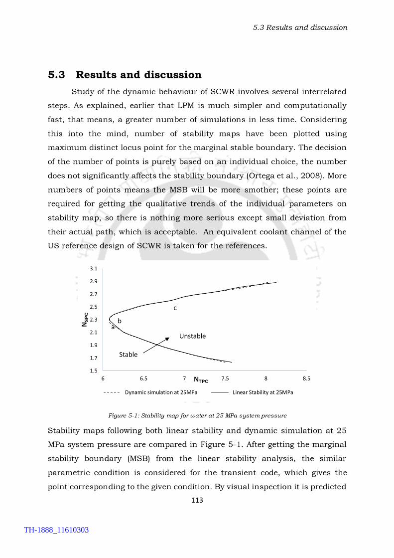
5.3 Results and discussion
113
5.3 Results and discussion
Study of the dynamic behaviour of SCWR involves several interrelated
steps. As explained, earlier that LPM is much simpler and computationally
fast, that means, a greater number of simulations in less time. Considering
this into the mind, number of stability maps have been plotted using
maximum distinct locus point for the marginal stable boundary. The decision
of the number of points is purely based on an individual choice, the number
does not significantly affects the stability boundary (Ortega et al., 2008). More
numbers of points means the MSB will be more smother; these points are
required for getting the qualitative trends of the individual parameters on
stability map, so there is nothing more serious except small deviation from
their actual path, which is acceptable. An equivalent coolant channel of the
US reference design of SCWR is taken for the references.
Figure 5-1: Stability map for water at 25 MPa system pressure
Stability maps following both linear stability and dynamic simulation at 25
MPa system pressure are compared in Figure 5-1. After getting the marginal
stability boundary (MSB) from the linear stability analysis, the similar
parametric condition is considered for the transient code, which gives the
point corresponding to the given condition. By visual inspection it is predicted
1.5
1.7
1.9
2.1
2.3
2.5
2.7
2.9
3.1
6 6.5 7 7.5 8 8.5
NS
PC
NTPC
Dynamic simulation at 25MPa Linear Stability at 25MPa
Stable
ab
c
Unstable
TH-1888_11610303

5.3 Results and discussion
114
that after some oscillations the system converges to its initial value, the
corresponding value is marked as a point for MSB. Now, similar simulations
are done for various inlet temperatures, the points obtained are then plotted
as the MSB and termed as dynamic simulation. Both the maps exhibit
amicable agreement. Figure 5-2 shows the comparison between two boundary
conditions with identical inlet. The system behaviour is different in both the
cases, which may be due to their different flow dynamics. However, the
pressure drop boundary condition is considered in the present analysis
because it is more realistic. For low levels of heater power, fluid temperature
fails to attain the pseudocritical value within the channel exit, thereby
ensuring a liquid-like representation of the fluid throughout the channel. As
the entire channel resembles the node, 1 of LPM, all thermophysical
properties exhibit small variations with temperature and hence the system
behaves in a stable manner. However, for intermediate to high power levels,
water crosses the pseudocritical point during its passage through the channel
and therefore suffers a substantial reduction in its density and other
transport properties Figure 5-2. Higher density and viscosity level in zone 1
results in significant frictional and gravitational pressure drop from the
channel inlet to the pseudocritical point. However, both components are
much smaller for the rest of the channel, with small increase in the
acceleration part. Accordingly, the first zone has to bear the major share of
the pressure drop imposed on the system. For low inlet temperatures, the
pseudocritical boundary appears quite close to the exit plane.
TH-1888_11610303

5.3 Results and discussion
115
Figure 5-2: Comparisons of stability map at 25 MPa for thermal hydraulic in two different boundary conditions
Figure 5-3: Variation of Viscosity and density with inlet temperature of water at 25 MPa
For any given heater power, as the inlet temperature increases, the
pseudocritical boundary starts shifting towards inlet of channel. The system
is stable for low and high inlet temperatures, when the pseudocritical
boundary is close to the channel outlet and inlet, respectively. For
intermediate inlet temperatures, when the pseudocritical boundary is in the
1.0
1.5
2.0
2.5
3.0
0 2 4 6 8 10
NS
PC
NTPC
Mass flow B.C at 25MPa
Pressure drop B.Cat 25MPa
Stable
20
30
40
50
60
70
80
90
100
110
500 600 700 800
Vis
co
sit
y (
µP
a-s
)
Temperature (K)
Viscosity of Water at25 MPa
0
100
200
300
400
500
600
700
800
900
500 600 700 800
De
nsit
y (
kg
/m3)
Temperature (K)
Density of Water at 25MPa
Unstable
TH-1888_11610303

5.3 Results and discussion
116
middle of the channel, the system exhibits flow instabilities. These
instabilities are similar to density wave oscillations (DWO) in boiling channels,
which is the most common type of instability (Prasad et al., 2007). They take
place because of phase lag and feedback between flow rate, density, and
pressure drop. The main cause of DWO is the wave resulting from
perturbation in enthalpy, which travels at speed much lower than the speed
of propagation of the pressure disturbances. A periodic disturbance of the
inlet mass flow rate will lead to the oscillation of the pseudocritical boundary.
The pressure drops in the first zone and second zone will then oscillate. These,
along with mass flux oscillations, will lead to perturbations in density, which
travel downstream at velocities that are approximately equal to the second
zone fluid velocity. The pressure perturbation, however, travels much faster,
at the velocity of sound. Phase lag will thus occur among the oscillating
parameters, and these can lead to oscillations of the mass flow rate.
5.3.1 Transients simulations
Figure 5-4: Stable response of SCWR corresponding to point ‘a’ in the stability map at 25 MPa system pressure, 1843 kg/s mass flow rate and 0.32 MW/Channel input power
The discussion in Section (3.7.1) substantiates the success of the linear
stability analysis in predicting the stability threshold. However, to
comprehend the nature of instability, transient simulations are performed at
some selected operating conditions shown by three doted points named as a,
b and c in Figure 5-1. A small perturbation is imposed on inlet mass flow
0.114
0.115
0.116
0.117
1900 1905 1910 1915 1920
Zp
c*
Non-dimensional time
0.98
1.00
1.02
1.04
1.06
0.990 0.995 1.000 1.005 1.010
Gp
c*
Go*
TH-1888_11610303

5.3 Results and discussion
117
under constant channel pressure drop condition and corresponding temporal
profiles of system variables are followed over a sufficiently long interval. The
variation in 𝑧𝑝𝑐∗ for a typically stable system is presented in Figure 5-4, along
with the concerned phase-portrait on 𝐺𝑝𝑐∗ − 𝑧𝑝𝑐
∗ plane; a point ‘a’ shows this. It
is evident that the oscillations subside quite early and the profile continues
with a near-constant value. Corresponding phase portrait exhibits converging
spirals into a stable fixed point. Temporal development of 𝑧𝑝𝑐∗ for a system in
vicinity of the marginal stable boundary, which is shown by point ‘b’ in Figure
5-5. Hardly any distinguishable change can be observed in the amplitude of
oscillation over the considered time span. This indicates the stable limit cycle.
Corresponding phase portrait assumes the shape of a near-perfect circle,
beyond some period of initial development. At some point ‘c’ far from the limit
cycle it’s detected that, with small increase in the input power, oscillations
with growing amplitude can be observed (Figure 5-6). The portrait on the
state-space plane exhibits a spiral, diverging away from a stable fixed point
for a typically unstable system.
Figure 5-5: Neutrally stable response of SCWR corresponding to point ‘b’ in the stability map at 25 MPa system pressure, 1843 kg/s mass flow rate and 0.35 MW/Channel input power
0.107
0.108
0.109
0.11
0.111
1900 1905 1910 1915 1920
Zp
c*
Non-dimensional time
0.98
1.00
1.02
1.04
1.06
0.994 0.998 1.002 1.006 1.010
Gp
c*
Go*
TH-1888_11610303
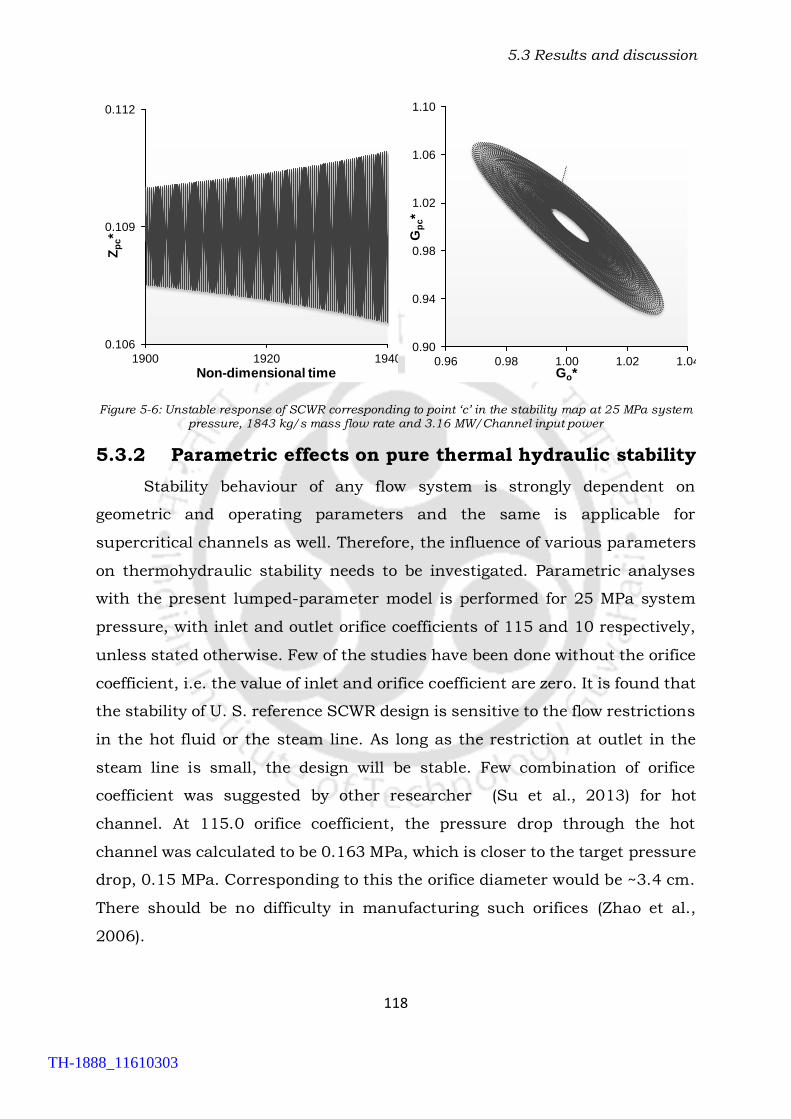
5.3 Results and discussion
118
Figure 5-6: Unstable response of SCWR corresponding to point ‘c’ in the stability map at 25 MPa system pressure, 1843 kg/s mass flow rate and 3.16 MW/Channel input power
5.3.2 Parametric effects on pure thermal hydraulic stability
Stability behaviour of any flow system is strongly dependent on
geometric and operating parameters and the same is applicable for
supercritical channels as well. Therefore, the influence of various parameters
on thermohydraulic stability needs to be investigated. Parametric analyses
with the present lumped-parameter model is performed for 25 MPa system
pressure, with inlet and outlet orifice coefficients of 115 and 10 respectively,
unless stated otherwise. Few of the studies have been done without the orifice
coefficient, i.e. the value of inlet and orifice coefficient are zero. It is found that
the stability of U. S. reference SCWR design is sensitive to the flow restrictions
in the hot fluid or the steam line. As long as the restriction at outlet in the
steam line is small, the design will be stable. Few combination of orifice
coefficient was suggested by other researcher (Su et al., 2013) for hot
channel. At 115.0 orifice coefficient, the pressure drop through the hot
channel was calculated to be 0.163 MPa, which is closer to the target pressure
drop, 0.15 MPa. Corresponding to this the orifice diameter would be ~3.4 cm.
There should be no difficulty in manufacturing such orifices (Zhao et al.,
2006).
0.106
0.109
0.112
1900 1920 1940
Zp
c*
Non-dimensional time
0.90
0.94
0.98
1.02
1.06
1.10
0.96 0.98 1.00 1.02 1.04
Gp
c*
Go*
TH-1888_11610303

5.3 Results and discussion
119
Figure 5-7: Effect of channel length on non-dimensional plain
Figure 5-8: Effect of channel length, Inlet temperature verses power
5.3.2.1 Effect of length
The effect of channel length on the stability threshold is presented in
Figure 5-7 and Figure 5-8. For a given inlet temperature, neutral stability
curve shifts towards lower power level with increase in channel length. In
Figure 5-7 and Figure 5-8, the neutral stability boundary is shown for various
1.5
1.7
1.9
2.1
2.3
2.5
2.7
2.9
3.1
7 8 9 10 11 12
NS
PC
NTPC
L=3.50 m
L=5.00 m
L=4.27 m
Stable
Unstable
300
350
400
450
500
550
0.15 0.2 0.25 0.3 0.35
Tin
(K)
Power(MW)
L=3.50 m
L=4.27 m
L=5.00 m
Stable
Unstable
TH-1888_11610303

5.3 Results and discussion
120
heated lengths (𝐿) in the stability map. Increasing the heated length creates a
destabilizing effect (𝐿= 3.50 m, 𝐿 = 4.27 m and 𝐿 = 5.00 m). This phenomenon
can be explained based on the gravitational and frictional pressure drop in
the momentum equation. It can be noticed that for a given inlet temperature
and power for three different lengths, the frictional pressure drop decreases
by 0.4 times while the increase in gravitational pressure drop is 1.8 times for
𝐿 =3.50 m and 𝐿 =4.27 m for the fixed mass flow rate. Due to increase in
channel length, the mass flow rate reduced as pressure drop is a boundary
condition. Consequently, the pseudocritical point shifted towards the inlet of
the channel, hence the system is unstable (Zhao et al., 2006). On the other
hand, increasing the length also extends the second zone, thereby causes an
unstable effect.
5.3.2.2 Effect of hydraulic diameter
Furthermore, the effect of the hydraulic diameter (𝐷ℎ) of the coolant
channel on the margins for instability is analysed. Figure 5-9 and Figure 5-10
shows the neutral stability boundary for various hydraulic diameters in non-
dimensional and in dimensional form, for 𝐷ℎ = 2.5, 3.4 and 4.0 mm. The
corresponding neutral stability boundary with a hydraulic diameter for a fuel
assembly of SCWR is given in solid line. Increasing the hydraulic diameter
has a stabilizing effect. This same kind of nature has been observed by Ortega
et al. ( 2008). It has to be noted that a typical fuel assembly of a supercritical
US reference design of SCWR have a hydraulic diameter of 𝐷ℎ = 3.4 mm (Zhao
et al., 2005).
TH-1888_11610303

5.3 Results and discussion
121
Figure 5-9: Effect of channel hydraulic diameter on non-dimensional plain without orifice coefficient
Figure 5-10: Effect of channel hydraulic diameter, Inlet temperature verses power plain
5.3.2.3 Effect of orifice coefficients
An inlet orifice coefficient always stabilized the system strongly, as
Figure 5-11 and Figure 5-12 shows. This is similar to the phenomena in BWR.
In the two-phase system the stability boundary depends on the pressure loss
distribution in heavy fluid region (i.e. before the boiling boundary reached, or
the subcooled liquid) and the region of lighter fluid which is above the boiling
boundary on the other hand, for the super critical case, the subcooled liquid
1.5
1.7
1.9
2.1
2.3
2.5
2.7
2.9
3.1
6 7 8 9 10 11 12
Nsp
c
Ntpc
Dia 2.50mm
Dia-3.40mm
Dia 4.00mm
300
350
400
450
500
550
0.1 0.15 0.2 0.25 0.3
Tin
(K)
Power(MW)
Dia.=2.50 mm
Dia.=3.40 mm
Dia.=4.00 mmStable
Unstable
TH-1888_11610303

5.3 Results and discussion
122
region corresponds to the high-density region before the fluid is heated
beyond the pseudo-critical point. Any device, which increases the pressure
loss of the heavy liquid region, increases the so-called in-phase pressure loss.
On the contrary, the effect of a flow resistance at the channel outlet (or also
called out-of-phase pressure loss) is strongly destabilizing. Strong care must
be taken with pressure losses at the outlet or the upper part of the coolant
channel. Since an in-phase pressure loss is the most sensitive parameter for
stabilizing a supercritical flow channel, inlet orifices coefficient can be
customized to assure stable operation with respect to DWOs for otherwise
unstable channels.
Figure 5-11: Effect of inlet and outlet orifice coefficient stability map
1.5
1.7
1.9
2.1
2.3
2.5
2.7
2.9
3.1
7 12 17 22
NS
PC
NTPC
Kin=110, Ko=1.0
Kin=110, Ko=1.5
Kin=120, Ko=10.0
Kin=100, Ko=10.0
Kin=110, Ko=10.0
Stable
Unstable
TH-1888_11610303
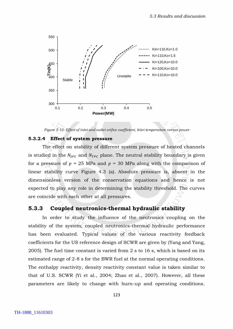
5.3 Results and discussion
123
Figure 5-12: Effect of inlet and outlet orifice coefficient, Inlet temperature verses power
5.3.2.4 Effect of system pressure
The effect on stability of different system pressure of heated channels
is studied in the 𝑁𝑆𝑃𝐶 and 𝑁𝑇𝑃𝐶 plane. The neutral stability boundary is given
for a pressure of 𝑝 = 25 MPa and 𝑝 = 30 MPa along with the comparison of
linear stability curve Figure 4.3 (a). Absolute pressure is, absent in the
dimensionless version of the conservation equations and hence is not
expected to play any role in determining the stability threshold. The curves
are coincide with each other at all pressures.
5.3.3 Coupled neutronics-thermal hydraulic stability
In order to study the influence of the neutronics coupling on the
stability of the system, coupled neutronics-thermal hydraulic performance
has been evaluated. Typical values of the various reactivity feedback
coefficients for the US reference design of SCWR are given by (Yang and Yang,
2005). The fuel time constant is varied from 2 s to 16 s, which is based on its
estimated range of 2-8 s for the BWR fuel at the normal operating conditions.
The enthalpy reactivity, density reactivity constant value is taken similar to
that of U.S. SCWR (Yi et al., 2004; Zhao et al., 2007). However, all these
parameters are likely to change with burn-up and operating conditions.
300
350
400
450
500
550
0.1 0.2 0.3 0.4 0.5
Tin
(K)
Power(MW)
Kin=110,Ko=1.0
Ki=110,Ko=1.5
Ki=120,Ko=10.0
Ki=100,Ko=10.0
Ki=110,Ko=10.0
StableUnstable
TH-1888_11610303

5.3 Results and discussion
124
Further, in order to investigate their influence on the low frequency
thermohydraulic oscillations, all these parameters have been varied to study
their influence on the instability, similar to parametric studies on BWR (Nayak
et al., 2000).
5.3.3.1 Effect of fuel time constant
The effect of fuel time constant on the stability of SCWR is shown Figure
5-13. The fuel time constant will vary depending on the fuel properties and
operational conditions. Van der Hagen (1998) has shown that with the use of
lumped parameter model it could be achievable. The fuel time constant, in
the present analysis, has been varied over a wide range from its normal
operating value to study its influence on the stability. The stability of the
reactor decreases with increase in fuel time constant. Previous studies on
BWR (March-Leuba and Rey, 1993; Nayak et al., 2000) have shown that
changes in fuel time constant have both stabilising and destabilising effects.
It was found that the stabilising effect is due to the inherent filtering of high
frequency oscillations, and the destabilising effect is due to the phase delay
to the feedback. For the moderate frequency thermohydraulic oscillations
observed in the SCWR, the phase delay is more significant to destabilise the
reactor for an increase in fuel time constant than the filtering effect (Chaudri
et al., 2013; Zhao et al., 2006 a,b).
TH-1888_11610303

5.3 Results and discussion
125
Figure 5-13: Effect of Fuel time constant at pressure 25MPa and enthalpy reactivity coefficient is –0.005
Figure 5-14: Effect of enthalpy Reactivity Coefficient at pressure 25MPa and fuel time constant 8 s.
5.3.3.2 Effect of enthalpy reactivity coefficient
The enthalpy reactivity coefficient depends on the core design, while the
Doppler coefficient is almost constant (Yang and Yang, 2005). From the
viewpoint of plant control, it should not be too large or too small. If it is too
large, the SCWR is unstable and the controllability is worse because the power
is more sensitive to the flow rate. On the other hand, if it is too small, the
1.7
1.9
2.1
2.3
2.5
2.7
2.9
3.1
6.5 7.5 8.5 9.5 10.5
NS
PC
NTPC
Fuel time constant = 16.0 s
Fuel time constant = 8.0 s
Fuel time constant = 2.0 s
Stable
Unstable
1.7
1.9
2.1
2.3
2.5
2.7
2.9
3.1
10.0 12.0 14.0 16.0 18.0
NS
PC
NTPC
Enthalpy reactivity coefficient= -0.02
Enthalpy reactivity coefficient= -0.005
Enthalpy reactivity coefficient= -0.0
Unstable
TH-1888_11610303

5.4 Conclusions
126
controllability is also worse because the density feedback is smaller and then
the main steam temperature is more sensitive to the flow rate (Ishiwatari et
al., 2003). Figure 5-14, shows the effect of enthalpy reactivity coefficient on
the threshold of stability for the SCWR reactor. The stability of the reactor is
found to increase with an increase in the absolute value of the negative
enthalpy reactivity coefficient. Results from previous investigations for vessel
type BWRs have shown that the stability of the reactor decreases with
increase in negative enthalpy reactivity coefficient due to the increase in gain
of the void reactivity feedback loop (Uehiro et al., 1996; van Bragt and van der
Hagen, 1998). (Nayak et al., 2000), observed that by addition of neutronics
feedback at such low frequency of thermo- hydraulic oscillations (<0.07 Hz)
which was studied by them for AHWR system, stabilises the reactor due to
less phase lag between the fuel heat generation rate and channel
thermohydraulic oscillations. The similar phenomena has been observed in
SCWR.
5.4 Conclusions
The present study employs a simplified lumped parameter model (LPM)
for stability evaluation of SCWR. Stability maps predicated by the transient
simulation with LPM and linear stability analysis show excellent match, as
expected. Further, there is qualitative match between the stability maps
prepared using LPM and RELAP5. Parametric effects on the stability threshold
have been investigated and major conclusions are the following.
a) Increasing the heated channel length has destabilizing effect on the
system, which is quite common in boiling channels also.
b) Stabilizing effect on the system has been observed by increasing the
hydraulic diameter with and without orifice coefficient.
c) Increase in inlet orifice coefficient has stabilizing effect whereas the
reverse can be observed for the outlet orifice.
d) System pressure is found to have negligible effect on the non-
dimensional stability threshold.
TH-1888_11610303

5.4 Conclusions
127
e) The stability of the reactor decreases with increase in fuel time
constant.
f) The stability of the reactor is found to increase with an increase in
negative enthalpy reactivity coefficient.
The results reported here predict the stability behaviour of the SCWR,
considering thermal hydraulics, fuel rod dynamics, and power dynamics.
TH-1888_11610303

5.4 Conclusions
128
TH-1888_11610303
6.1 Introduction
129
STABILITY ANALYSIS OF SCWR
USING THREE ZONE LPM
6.1 Introduction
Instability analysis is very important for the safely of the SCWR. To
analysis these aspects, two zone LPM has been developed (section 3.2). As it
is the simplified model, and gives the qualitative information about the system
stability. Therefore, to know the extents of stability margin by increasing the
numbers of nodes, the study has been done in this chapter using three zone
model. The model has been developed using the same concept, which has
been used in section (3.1). Moreover, using this model the instability has been
characterized. Earlier, in order to characterize such instabilities, the concept
of two-region model comprising of (i) a “liquid like region” and (ii) a “gas like
region” is used (Zuber, 1966). The transition between the two regions was
identified by the appearance of the pseudocritical point. An improvement on
that in the form of a three-region model was later proposed, which was found
to provide reasonably better prediction on the stability prediction of SCWR.
Therefore, present study carries out a lumped parameter base stability
analysis for a heated channel with supercritical fluid following three-region
model. In the present model stability analysis has been done on three
geometrical parameters and their detailed stability map has been plotted for
locating the stable and unstable zones.
Zhang et al., (2015) proposed a three-region model to investigate the density
wave instabilities of SCW in tubes, where a specific region of SCW was defined
as “two-phase mixture”, and the demarcation points of three regions were the
pseudo critical point and a point with “latent heat” of 400 kJ/kg. The three
region model was proved better than the two region one considering some
limitations. Zhao et al., (2005) proposed another three-region model for the
analyses of density wave instabilities of SCW in tubes, on the basis of the
partition method different. A linear stability analysis code in the frequency
TH-1888_11610303

6.1 Introduction
130
domain was developed by many researchers (Yi et al., 2004; Yoo et al., 2006)
to study the thermal-hydraulic stability of the supercritical pressure light
water reactor at constant supercritical pressure. Then, the thermal-hydraulic
stability of super- critical pressure light water reactor for both full-power
condition and partial-power condition was investigated. To carry out the
steady state and linear stability analysis of a SCW natural circulation loop,
(Sharma et al., 2013) proposed a computer code by using supercritical water
properties. However, because of the complexity of the physical properties of
SCW, there is still not a unified model for studying the instabilities of SCW
flows in tubes. Concerning the previous studies as mentioned above, the three
commonly used mathematical models for the study of density wave
instabilities of SCW flows are carried out (Zhang et al., 2015; Zuber, 1966),
which is based on frequency domain method. The three models are derived
based on the different partition methods of SCW. Detailed information is
shown in the following section.
Under subcritical pressures, the flow region in a tube was usually divided into
three parts, i.e., the preheating region, the boiling region and the
superheating region, for studying density wave instability. Considering the
similar features of subcritical water and SCW, the models derived at the
subcritical pressure may also be employed for the relevant study at the
supercritical pressure, if the flow region in tubes at the supercritical pressure
could be divided into three parts just like that at the subcritical pressure.
Many efforts had been carried out in the recent decades (Zhang et al., 2015;
Zuber, 1966) and different models were established for the study on density
wave instability of SCW in tubes, based on the models used for subcritical
conditions. The three commonly used mathematical models were from (Zhang
et al., 2015; Zuber, 1966), respectively. The primary differences among the
three models were the regional partitions of SCW. The different regional
partitions in the three methods are simply expressed as follows, and are
described using graphs in the same form to facilitate the comparisons. Zhang
et al. (2015) compared the above three model and suggested some
TH-1888_11610303

6.2 Mathematical modelling
131
improvements by increasing the second region area which reduced the relative
error of the present model by 26%, while that of the other three models are all
greater than 30%.
In the present analysis, the main focused is to analyses the thermal
hydraulics parameter by using the improved three zone lumped parameter
model (LPM) (Zhang et al., 2015). The parameters which have been varied for
the study are channel length, hydraulic diameter and inlet and outlet orifice
coefficients. Transient plot and stability map has been plotted for these
parameters which further supports the stability analysis. However, the
detailed analysis has been done by considering two different values of the
geometrical parameter and three different values for orifice coefficient apart
from the design values.
6.2 Mathematical modelling
The reactor core has been divided in three separated regions (Figure
6-1), namely, (1) liquid-like heavy fluid region with constant density, (2)
mixture region of heavier and lighter fluid behaving similar to a homogeneous
two-phase mixture and (3) gas-like lighter fluid with constant density. The
basic dimensional conservation equations (3.1-3.3) are similar to the two zone
model, finally using the nondimensional parameters equation (6.1) as in
dimensional equations,
𝑧∗ =𝑧
𝐿𝑐, 𝑡∗ =
𝑡𝐺𝑐
𝜌𝑝𝑐𝐿𝑐, 𝐺∗ =
𝐺
𝐺𝑐, 𝜌∗ =
𝜌 − 𝜌𝑝𝑐
𝜌𝑝𝑐, 𝑝∗ =
(𝑝 − 𝑝𝑟)𝜌𝑝𝑐
𝐺𝑐2
, 𝑇∗
=𝑇 − 𝑇𝑝𝑐
𝑇𝑝𝑐
, ℎ∗ =(ℎ − ℎ𝑝𝑐)
ℎ𝑝𝑐
, 𝑁𝐹𝑟 =𝐺𝑐
2
𝜌𝑝𝑐2 𝑔𝐿𝑐
, 𝑁𝑇𝑃𝐶
=𝑞0
′′𝜋ℎ𝐿𝑐
𝐴𝐺𝑐
𝛽𝑝𝑐
𝐶𝑝.𝑝𝑐
, 𝑁𝐸𝑢 =𝑓𝐿𝑐
2𝐷ℎ
6.1
Which finally gives equations (6.2-6.4).
TH-1888_11610303

6.2 Mathematical modelling
132
𝜕𝜌∗
𝜕𝑡∗+
𝜕𝐺∗
𝜕𝑧∗= 0
6.2
𝜕𝐺∗
𝜕𝑡∗+
𝜕
𝜕𝑧∗(𝐺∗2
𝜌∗) = −
𝜕𝑝∗
𝜕𝑧∗−
𝜌∗ − 1
𝑁𝐹𝑟
− [𝑁𝐸𝑢 + 𝐾𝑖𝛿∗(𝑧∗) + 𝐾𝑜𝛿∗(𝑧∗ − 1)]
𝐺∗2
𝜌∗
6.3
𝜕
𝜕𝑡∗(𝜌∗ℎ∗) +
𝜕
𝜕𝑧∗(𝐺∗ℎ∗) = 𝑁𝑇𝑃𝐶 𝑓(𝑡∗)
6.4
Figure 6-1: Schematic view of the heated channel following by three-region model
The above equations are then integrated separately over each of the regions,
while incorporating suitable equation of state.
6.2.1 Equations of state (EOS)
Due to lots of anomalies between two-zone and three-zone model and
that also on the cost of stability, is preliminary based on the EOS. However,
observing the method by which Zhao et al., (2006) divided the model into
three-zone, the following two major glitches have been observed. Firstly, TPSW
which is the temperature at the boundary of H-F and H-L-M is defined as a
constant, equalling to 350 oC. It is obvious that near the small zone where the
density varies sharply at different pressures does not have the same starting
TH-1888_11610303

6.2 Mathematical modelling
133
point. It means that TPSW changes with the pressure, and defining TPSW as a
constant is not so appropriate. Secondly, the temperature of the exit
delineation between H-L-M and L-F is somewhat low, which is approximately
450 oC. In SCWR the exit, temperature is greater than 500 oC. So, a more
practical method must have needed.
Hence, considering these gapes, a more general and resolute relations have
been proposed. The relations levee the aforementioned breaks. These
equations of state for each of the regions are obtained by fitting a piecewise
linear function with IAPWS data of water at 25MPa (Figure 6-2), which is given
as below.
𝜌∗ = −2.21ℎ∗ + 0.49 𝑓𝑜𝑟 − 0.6 < ℎ∗ ≤ −0.3
6.5 𝜌∗ =−3.6683 ℎ∗ 𝑓𝑜𝑟 −0.3 ≤ ℎ∗ ≤ 0.05
𝜌∗ =−2.11ℎ∗ − 0.0363 𝑓𝑜𝑟 0.05 ≤ ℎ∗
Figure 6-2: Fitting of equation of state with IAPWS data of water at 25 MPa.
6.2.2 Enthalpy profile and relation between 𝝆∗ and 𝒉∗
Assuming a linear enthalpy variation with axial coordinate the following
relations hold for the first, second and third node.
-1.0
-0.5
0.0
0.5
1.0
1.5
2.0
-0.7 -0.6 -0.5 -0.4 -0.3 -0.2 -0.1 0 0.1 0.2 0.3 0.4
ρ*
h*
Water 1st Region 2nd Region 3rd Region
TH-1888_11610303

6.2 Mathematical modelling
134
ℎ∗ = (ℎ1∗ − ℎ𝑖
∗)𝑧∗
𝑧1∗ + ℎ𝑖
∗
ℎ∗ = [ℎ1
∗ − ℎ2∗
𝑧1∗ − 𝑧2
∗ ] (𝑧∗ − 𝑧1∗) + ℎ1
∗
ℎ∗ = [ℎ2
∗ − ℎ𝑜∗
𝑧2∗ − 1
] (𝑧∗ − 1) + ℎ𝑜∗
6.6
Where ℎ1∗ and ℎ2
∗ are the non-dimensional enthalpy at the boundaries of the
two regions.
Using the property relations into the non-dimensional governing equations
and integrating the equation for three different zone for the equation of state
variables. The mass and energy equations are further integrated over region
1st from inlet to Z1, which gives one ODEs and one algebraic equation.
𝑑𝑧1∗
𝑑𝑡∗=
𝐺𝑖∗ − 𝐺1
∗
𝐴1
𝐺1∗ =
𝑁𝑇𝑃𝐶𝑀𝑧1∗𝐴1 + 𝐺𝑖
∗ℎ𝑖∗𝐴1 − 𝐺𝑖
∗𝐵1
ℎ1∗ − 𝐵1
6.7
Where, 𝐴1 =𝑎1(ℎ1
∗−ℎ𝑖∗)
2+ (𝑎1ℎ𝑖
∗ + 𝑏1) − (𝑎1ℎ1∗ + 𝑏1)
𝐵1 = 𝑎1ℎ𝑖∗(ℎ1
∗ − ℎ𝑖∗) + 𝑎1ℎ𝑖
∗2 +𝑏1(ℎ1
∗ − ℎ𝑖∗)
2+ 𝑏1ℎ𝑖
∗ − (𝑎1ℎ1∗ + 𝑏1)ℎ1
∗
𝐶1 = 1 + 𝑏1
In the same way, mass and energy equations are integrating over region 2 i.e.
from Z1 to Z2, which gives an ODEs and an algebraic equation
𝑑𝑧2∗
𝑑𝑡∗=
𝐺1∗ − 𝐺2
∗ − 𝐷2𝑑𝑧1
∗
𝑑𝑡∗
𝐶2
𝐺2∗ =
𝑁𝑇𝑃𝐶𝑀𝐶2(𝑧2∗ − 𝑧1
∗)𝐶1 − 𝐺1∗(ℎ1
∗𝐶2 − 𝐴2) + (𝐷2𝐴2 − 𝐵2𝐶2)𝑑𝑧1
∗
𝑑𝑡∗
(ℎ2∗𝐶2 − 𝐴2)
6.8
TH-1888_11610303
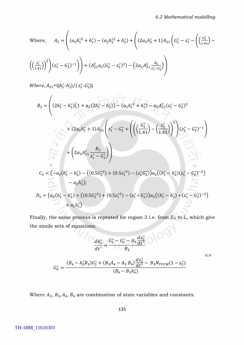
6.2 Mathematical modelling
135
Where, 𝐴2 = ((𝑎2ℎ1∗2 + ℎ1
∗) − (𝑎2ℎ2∗2 + ℎ2
∗) + ((2𝑎2ℎ2∗ + 1)𝐴21 (𝐺2
∗ − 𝑧1∗ − ((
𝐺2∗
1.41) −
((𝑧1
∗
1.41))
2
)(𝑧1∗ − 𝐺2
∗)−1)) + (𝐴212 𝑎2(𝐺2
∗ − 𝑧1∗)2) − (2𝑎2𝐴21
2 𝐵2
𝑧1∗−𝐺2
∗))
𝑊ℎ𝑒𝑟𝑒, 𝐴21=((ℎ1∗-ℎ2
∗ )/( 𝑧1∗-𝐺2
∗))
𝐵2 = ((2ℎ1∗ − ℎ2
∗)(1 + 𝑎2(2ℎ1∗ − ℎ2
∗)) − (𝑎2ℎ1∗2 + ℎ1
∗) − 𝑎2𝐴212 (𝑧1
∗ − 𝐺2∗)2
+ (2𝑎2ℎ1∗ + 1)𝐴21 (𝑧1
∗ − 𝐺2∗ + (((
𝐺2∗
1.41) − (
𝑧1∗
1.41))
2
) (𝑧1∗ − 𝐺2
∗)−1)
+ (2𝑎2𝐴212
𝐵2
𝑧1∗ − 𝐺2
∗))
𝐶2 = (−𝑎2(ℎ1∗ − ℎ2
∗) − ((0.5𝐺2∗2) + (0.5𝑧1
∗2) − (𝑧1∗𝐺2
∗))𝑎2((ℎ1∗ − ℎ2
∗)(𝑧1∗ − 𝐺2
∗)−2)
− 𝑎2ℎ2∗);
𝐷2 = (𝑎2(ℎ1∗ − ℎ2
∗) + ((0.5𝐺2∗2) + (0.5𝑧1
∗2) − (𝑧1∗ ∗ 𝐺2
∗))𝑎2((ℎ1∗ − ℎ2
∗) ∗ (𝑧1∗ − 𝐺2
∗)−2)
+ 𝑎1ℎ1∗)
Finally, the same process is repeated for region 3 i.e. from Z2 to L, which give
the simile sets of equations.
𝑑ℎ𝑜∗
𝑑𝑡∗=
𝐺2∗ − 𝐺𝑜
∗ − 𝐴3𝑑𝑧2
∗
𝑑𝑡∗
𝐵3
𝐺𝑂∗ =
(𝐵4 − ℎ2∗𝐵3)𝐺2
∗ + (𝐵3𝐴4 − 𝐴3 𝐵4)𝑑𝑧2
∗
𝑑𝑡∗ − 𝐵3𝑁𝑇𝑃𝐶𝑀(1 − 𝑧2∗)
(𝐵4 − 𝐵3ℎ𝑜∗)
6.9
Where 𝐴3, 𝐵3, 𝐴4, 𝐵4 are combination of state variables and constants.
TH-1888_11610303
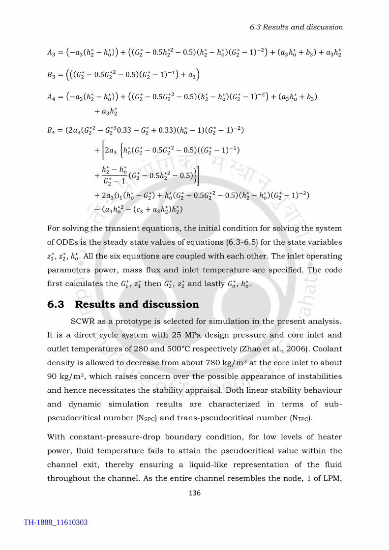
6.3 Results and discussion
136
𝐴3 = (−𝑎3(ℎ2∗ − ℎo
∗)) + ((𝐺2∗ − 0.5ℎ2
∗2 − 0.5)(ℎ2∗ − ℎo
∗)(𝐺2∗ − 1)−2) + (𝑎3ℎo
∗ + 𝑏3) + 𝑎3ℎ2∗
𝐵3 = (((𝐺2∗ − 0.5𝐺2
∗2 − 0.5)(𝐺2∗ − 1)−1) + 𝑎3)
𝐴4 = (−𝑎3(ℎ2∗ − ℎo
∗)) + ((𝐺2∗ − 0.5𝐺2
∗2 − 0.5)(ℎ2∗ − ℎo
∗)(𝐺2∗ − 1)−2) + (𝑎3ℎo
∗ + 𝑏3)
+ 𝑎3ℎ2∗
𝐵4 = (2𝑎3(𝐺2∗2 − 𝐺2
∗30.33 − 𝐺2∗ + 0.33)(ℎo
∗ − 1)(𝐺2∗ − 1)−2)
+ [2𝑎3 {ℎo∗(𝐺2
∗ − 0.5𝐺2∗2 − 0.5)((𝐺2
∗ − 1)−1)
+ℎ2
∗ − ℎo∗
𝐺2∗ − 1
(𝐺2∗ − 0.5ℎ2
∗2 − 0.5)}]
+ 2𝑎3(i1(ℎo∗ − 𝐺2
∗) + ℎo∗(𝐺2
∗ − 0.5𝐺2∗2 − 0.5)(ℎ2
∗ − ℎo∗)(𝐺2
∗ − 1)−2)
− (𝑎3ℎo∗2 − (𝑐3 + 𝑎3ℎ2
∗)ℎ2∗)
For solving the transient equations, the initial condition for solving the system
of ODEs is the steady state values of equations (6.3-6.5) for the state variables
𝑧1∗, 𝑧2
∗, ℎ𝑜∗ . All the six equations are coupled with each other. The inlet operating
parameters power, mass flux and inlet temperature are specified. The code
first calculates the 𝐺1∗, 𝑧1
∗ then 𝐺2∗, 𝑧2
∗ and lastly 𝐺𝑜∗, ℎ𝑜
∗ .
6.3 Results and discussion
SCWR as a prototype is selected for simulation in the present analysis.
It is a direct cycle system with 25 MPa design pressure and core inlet and
outlet temperatures of 280 and 500°C respectively (Zhao et al., 2006). Coolant
density is allowed to decrease from about 780 kg/m3 at the core inlet to about
90 kg/m3, which raises concern over the possible appearance of instabilities
and hence necessitates the stability appraisal. Both linear stability behaviour
and dynamic simulation results are characterized in terms of sub-
pseudocritical number (NSPC) and trans-pseudocritical number (NTPC).
With constant-pressure-drop boundary condition, for low levels of heater
power, fluid temperature fails to attain the pseudocritical value within the
channel exit, thereby ensuring a liquid-like representation of the fluid
throughout the channel. As the entire channel resembles the node, 1 of LPM,
TH-1888_11610303

6.3 Results and discussion
137
all thermophysical properties exhibit small variations with temperature and
hence the system behaves in a stable manner. However, for intermediate to
high power levels, water crosses the pseudocritical point during its passage
through the channel and therefore suffers a substantial reduction in its
density and other transport properties. Higher density and viscosity level in
region 1 results in significant frictional and gravitational pressure drop from
the channel inlet to the pseudocritical point. However, both components are
much smaller for the rest of the channel, with small increase in the
acceleration part. Accordingly, the first zone has to bear the major share of
the pressure drop imposed on the system. For low inlet temperatures, the
pseudocritical boundary appears quite close to the exit plane. For any given
heater power, as the inlet temperature increases, the pseudocritical boundary
starts shifting towards inlet of the channel. The system is stable for low and
high inlet temperatures, when the pseudocritical boundary is reasonably
close to the channel outlet and inlet, respectively. For intermediate inlet
temperatures, however, when the pseudocritical boundary is in the middle of
the channel, the system exhibits flow instabilities. These instabilities are
similar to density wave oscillations (DWO) in boiling channels, which is the
most common type of instability(Pandey and Kumar, 2007; Prasad et al.,
2007). They take place because of phase lag and feedback between flow rate,
density, and pressure drop. The main cause of DWO is the wave resulting
from perturbation in enthalpy, which travels at speed much lower than the
speed of propagation of the pressure disturbances. A periodic disturbance to
the inlet mass flow rate will lead to the oscillation of the pseudocritical
boundary, enforcing oscillations in the pressure drops in both the zones.
These, along with mass flux oscillations, will lead to perturbations in density,
which travel downstream at velocities approximately equal to the second zone
fluid velocity. The pressure perturbation, however, travels much faster, at the
velocity of sound. Phase lag will thus occur among the oscillating parameters,
and these can lead to oscillations of the mass flow rate.
TH-1888_11610303
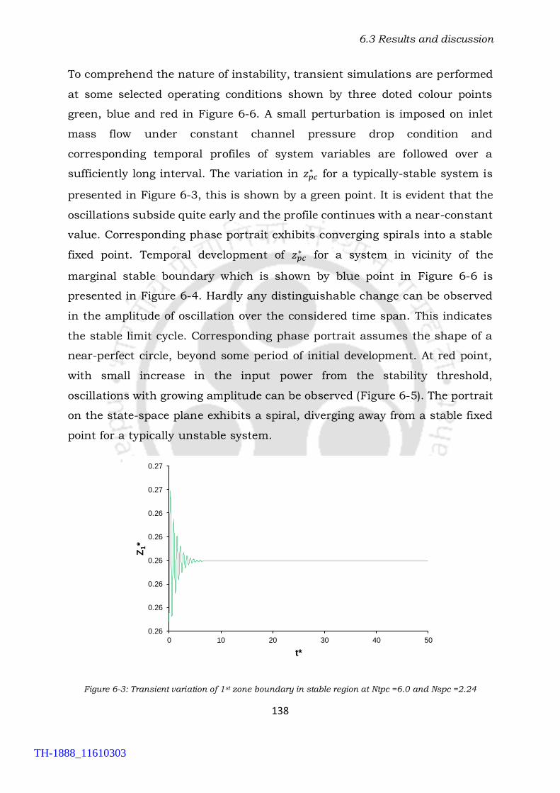
6.3 Results and discussion
138
To comprehend the nature of instability, transient simulations are performed
at some selected operating conditions shown by three doted colour points
green, blue and red in Figure 6-6. A small perturbation is imposed on inlet
mass flow under constant channel pressure drop condition and
corresponding temporal profiles of system variables are followed over a
sufficiently long interval. The variation in 𝑧𝑝𝑐∗ for a typically-stable system is
presented in Figure 6-3, this is shown by a green point. It is evident that the
oscillations subside quite early and the profile continues with a near-constant
value. Corresponding phase portrait exhibits converging spirals into a stable
fixed point. Temporal development of 𝑧𝑝𝑐∗ for a system in vicinity of the
marginal stable boundary which is shown by blue point in Figure 6-6 is
presented in Figure 6-4. Hardly any distinguishable change can be observed
in the amplitude of oscillation over the considered time span. This indicates
the stable limit cycle. Corresponding phase portrait assumes the shape of a
near-perfect circle, beyond some period of initial development. At red point,
with small increase in the input power from the stability threshold,
oscillations with growing amplitude can be observed (Figure 6-5). The portrait
on the state-space plane exhibits a spiral, diverging away from a stable fixed
point for a typically unstable system.
Figure 6-3: Transient variation of 1st zone boundary in stable region at Ntpc =6.0 and Nspc =2.24
0.26
0.26
0.26
0.26
0.26
0.26
0.27
0.27
0 10 20 30 40 50
Z1*
t*
TH-1888_11610303

6.3 Results and discussion
139
Figure 6-4: Transient variation of 1st zone boundary on marginal stable boundary Ntpc =6.13 and Nspc =2.24
Figure 6-5: Transient variation of 1st zone boundary in unstable region at Ntpc =6.28 and Nspc =2.24
6.3.1 Effect of length
The effect of channel length on the stability threshold is presented in
Figure 6-6. For a given inlet temperature, neutral stability curve shifts
towards lower power level with increase in channel length. In Figure 6-6, the
0.23
0.23
0.23
0.23
0.23
0.24
0.24
0.24
0.24
0 10 20 30 40 50
Z1*
t*
0.22
0.23
0.23
0.24
0.24
0.25
0.25
0 10 20 30 40 50
Z1*
t*
TH-1888_11610303

6.3 Results and discussion
140
neutral stability boundary is shown for various heated lengths (𝐿) in the
stability map. Increasing the heated length creates a destabilizing effect (𝐿=
3.50 m, 𝐿 = 4.27 m and 𝐿 = 5.00 m). This phenomenon can be explained on
the basis of the gravitational and frictional pressure drop in the momentum
equation. It can be noticed that for a given inlet temperature and power for
three different lengths, the frictional pressure drops decrease to 0.4 times,
while the increase in gravitational pressure drop is 1.8 times for 𝐿 =3.50 m
and 𝐿 =4.27 m for the fixed mass flow rate. Due to increase in the channel
length, the mass flow rate reduces, as pressure drop across the channel is a
predefined boundary condition. Consequently, the pseudocritical point shifts
towards the inlet of the channel, thereby destabilizing the system (Zhao et al.,
2006).
Figure 6-6: Stability map of three different channel length.
6.3.2 Effect of hydraulic diameter
Furthermore, the effect of the hydraulic diameter (Dh) of the coolant
channel on the margins for instability is analysed. Figure 6-7 shows the
neutral stability boundary for various hydraulic diameters in non-
1.5
2.0
2.5
3.0
5.0 6.0 7.0 8.0 9.0 10.0
Nsp
c
Ntpc
3.50m 4.27m 5.00m
Stable
Unstable
TH-1888_11610303

6.3 Results and discussion
141
dimensional and in dimensional form, for Dh = 2.5, 3.4 and 4.0 mm. The
corresponding neutral stability boundary with a hydraulic diameter for a fuel
assembly of SCWR is given in solid curve. Increasing the hydraulic diameter
has a stabilizing effect. Few of the irregular shapes in stability map have been
observed during the simulations, these are due to the change in the orifices
coefficients as observes in the two-zone model. In all the MSB there is a sharp
topological change which is only due to the change in the value of kin and kout
at that particular point. Two times per stability map, these changes have been
made. It has to be noted that a typical fuel assembly of a supercritical US
reference design of SCWR have a hydraulic diameter of Dh = 3.4 mm.
Figure 6-7: Stability map of three different channel hydraulic diameter.
6.3.3 Effects of orifice coefficients
An inlet orifice coefficient always stabilized the system strongly, as
Figure 6-8 shows. This is similar to the phenomena in BWR. In the two-phase
system the stability boundary depends on the pressure loss distribution in
heavy fluid region (i.e. before the boiling boundary reached, or the subcooled
liquid) and the region of lighter fluid which is above the boiling boundary on
the other hand, for the super critical case, the subcooled liquid region
corresponds to the high-density region before the fluid is heated beyond the
pseudo-critical point. Any device, which increases the pressure loss of the
heavy liquid region, increases the so-called in-phase pressure loss. On the
1.5
1.7
1.9
2.1
2.3
2.5
2.7
2.9
3.1
5 6 7 8 9 10
NS
PC
NTPC
Dia. 2.5 mm Dia. 3.4 mm Dia. 4.0 mm
TH-1888_11610303

6.3 Results and discussion
142
contrary, the effect of a flow resistance at the channel outlet (or also called
out-of-phase pressure loss) is strongly destabilizing. Strong care must be
taken with pressure losses at the outlet or the upper part of the coolant
channel. Since an in-phase pressure loss is the most sensitive parameter for
stabilizing a supercritical flow channel, inlet orifices coefficient can be
customized to assure stable operation with respect to DWOs for otherwise
unstable channels.
Figure 6-8: Stability map of four different sets of orifices coefficients
1.0
1.5
2.0
2.5
3.0
10 12 14 16 18 20
Ns
pc
Ntps
Ki 20, Ko 10 Ki 30, Ko 0 Ki 20, Ko 0 Ki 10, Ko 0
Stable
Unstable
TH-1888_11610303
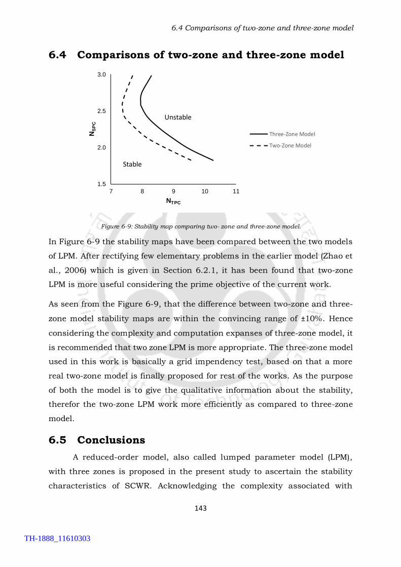
6.4 Comparisons of two-zone and three-zone model
143
6.4 Comparisons of two-zone and three-zone model
Figure 6-9: Stability map comparing two- zone and three-zone model.
In Figure 6-9 the stability maps have been compared between the two models
of LPM. After rectifying few elementary problems in the earlier model (Zhao et
al., 2006) which is given in Section 6.2.1, it has been found that two-zone
LPM is more useful considering the prime objective of the current work.
As seen from the Figure 6-9, that the difference between two-zone and three-
zone model stability maps are within the convincing range of ±10%. Hence
considering the complexity and computation expanses of three-zone model, it
is recommended that two zone LPM is more appropriate. The three-zone model
used in this work is basically a grid impendency test, based on that a more
real two-zone model is finally proposed for rest of the works. As the purpose
of both the model is to give the qualitative information about the stability,
therefor the two-zone LPM work more efficiently as compared to three-zone
model.
6.5 Conclusions
A reduced-order model, also called lumped parameter model (LPM),
with three zones is proposed in the present study to ascertain the stability
characteristics of SCWR. Acknowledging the complexity associated with
1.5
2.0
2.5
3.0
7 8 9 10 11
NS
PC
NTPC
Three-Zone Model
Two-Zone Model
Stable
Unstable
TH-1888_11610303

6.5 Conclusions
144
handling the complete set of conservation equations and numerical models
thereof, momentum and energy conservation equations are integrated
following the CI method, converting the PDEs to a set of algebraic equations
and ODEs. The resultant lumped parameter model is employed to envisage
both the linear and transient stability behavior of a heated supercritical
channel. Stability maps predicated by the transient simulation with LPM and
linear stability analysis show excellent match, as expected. Parametric effects
on the stability threshold have been investigated and major conclusions are
the following.
a) Increasing the heated channel length has destabilizing effect on the
system, which is quite common in boiling channels also.
b) Stabilizing effect on the system has been observed by increasing the
hydraulic diameter.
c) Increase in inlet orifice coefficient has stabilizing effect whereas the
reverse can be observed for the outlet orifice.
d) There is only ±10% enhancement in the MSB by using three-zone model
as compared to the two- zone, hence later one is more suitable for further
study.
The results reported here predict the stability behavior of the SCWR,
considering three-zone LPM only.
TH-1888_11610303

6.5 Conclusions
145
TH-1888_11610303

7.1 Introduction
146
NONLINEAR DYNAMICS AND
BIFURCATION ANALYSIS
7.1 Introduction
Supercritical water experiences effective changes in thermodynamically
and transport properties nearby the pseudocritical boundary. Therefore, the
SCWR will exhibit colossal variation in density across the core, creating it
assailable to density wave instability, similar to BWRs (Blázquez et al. 2013;
Gajev et al. 2013; Peng et al. 1986), compelling emphasis on passive safety
design. Consequently, a number of researchers have studied the stability
response of supercritical flow systems in the recent past following various
approaches, with more preference towards natural circulation loops.
The linear stability analysis is computationally fast, which locates marginal
stability boundary based on eigenvalue approach. Linear stability analysis
characterizes the system behaviour for small perturbation about the steady
state. In order to predict the nature of system transients following large
perturbations, it is necessary to conduct nonlinear stability analysis or
bifurcation analysis. While nonlinear stability analysis of boiling channels has
been done by several researchers (Prasad and Pandey, 2007; Mishra and
Singh, 2016), such analysis for SCWR is not found in the literature. This is
important because a subcritical Hopf bifurcation lead to an unstable limit
cycle, which is dangerous as it, makes the system unstable for large
perturbations. The autonomous shooting technique can be used to find the
exact location of an unstable limit cycle, as was done by (Durga Prasad and
Pandey, 2008). However, most of the researchers (for example, Mishra and
Singh, 2016) inferred the existence of an unstable limit cycle by simulating
the transients for small and large perturbations, and did not locate it in the
state space by the shooting method.
TH-1888_11610303

7.2 Mathematical modelling
147
Present work, therefore, focuses on understanding the thermohydraulic,
coupled neutronic-thermalhydraulic stability behaviour of a forced flow
heated channel carrying supercritical water, and envisages the effect of
associated system parameters on stability boundaries employing both linear
and nonlinear stability analysis. Reduced order models are computationally
less expensive compared to finite-difference-kind of approaches and hence are
often preferred to obtain a first estimate. Accordingly, a lumped parameter-
based approach is followed (Section 3.2), visualizing the channel to consist of
two distinct zones, separated by the pseudocritical point
7.2 Mathematical modelling
A round forced flow channel of uniform diameter is simulated in the
present study, under uniform heat flux imposed on the wall. The channel is
subjected to constant mass flow rate boundary condition in both steady and
transient conditions. Accordingly, the 1D conservation equations for mass,
momentum and energy can be summarized by Eq. (3.5-3.7) and finally using
equations from Section (3.4) for the transient study.
7.3 Results and discussion
In the present work, linear stability and nonlinear analysis (Section 3.6)
are carried out using in-house code based on the MATLAB and a software
MATCONT. The linear analysis provides the numbers of discreet points, which
are the locus of MSB at a particular pressure, in this case at 25 MPa. The L-
shaped stability map in the NTPC-NSPC space obtained from the analysis is
shown in Figure 7-1. This result is used in the following sections for analysis
of bifurcations, which lead to different types of dynamic behaviour of the
system. In order to verify the predictions of linear stability analysis, numerical
simulations of the system of ODEs (Eq. 3.1–3.3) are carried out for the design
operating conditions, using the MATLAB ODE solver ODE15s (Mcevoy, 2009).
7.3.1 Identification of generalized Hopf (GH) points
In this study, the bifurcation analysis has been carried out by using
MatCont (Dhooge et al. 2003; Mishra and Singh 2016; Meijer 2008). It
TH-1888_11610303

7.3 Results and discussion
148
provides a continuation and bifurcation toolbox, which is compatible with the
standard MATLAB ODEs representation of differential equations. The GH
point obtained for the system under study is shown in Figure 7-1. Hence, it
is predicted that the system will exhibit supercritical (soft and safe) and
subcritical (hard and dangerous) Hopf bifurcations, respectively, below and
above the GH point. This is verified by numerical simulations in the following
sections.
Figure 7-1: Stability map showing GH point on MSB
1.2
1.6
2.0
2.4
2.8
3.2
5.5 6.0 6.5 7.0 7.5 8.0 8.5 9.0
Nsp
c
Ntpc
A B
CD
Supercritical
SubcriticalGH
TH-1888_11610303

7.3 Results and discussion
149
Figure 7-2: Temporal variation of Zpc*
Figure 7-3: Temporal variation of Zpc*
0.13
0.13
0.13
0.13
0.13
0.13
0.13
0.13
0 2 4 6 8 10 12 14 16 18 20
Zp
c*
t*
0.09
0.1
0.11
0.12
0.13
0.14
0.15
0.16
0 1 2 3 4 5 6 7 8 9 10
Zp
c*
t*
TH-1888_11610303

7.3 Results and discussion
150
Figure 7-4: Phase portrait of Go*and Zpc*
Figure 7-5: Unstable temporal variation of Zpc* corresponding to point M
7.3.2 Numerical simulation analysis in supercritical region
Figure 7-3 represents the time evolution of pseudocritical boundary of
the coolant at parametric values corresponding to point D on Figure 7-1.
These points are in the unstable side of MSB as delineated by the linear
stability analysis. Therefore, for small perturbations, the oscillations are grow
with time (Figure 7-3). However, since point D is in the supercritical region,
0.99
1.00
1.00
1.01
1.01
1.02
1.02
0.12 0.122 0.124 0.126 0.128 0.13 0.132 0.134
Go*
Zpc*
0.06
0.08
0.10
0.12
0.14
0.16
0.18
0 1 2 3 4 5
Zp
c*
t*
TH-1888_11610303

7.3 Results and discussion
151
the oscillating trajectory ultimately follows a periodic orbit (Figure 7-4). This
indicates the existence of a stable limit cycle in the unstable region (as
predicted by linear stability analysis) which is the characteristic of a
supercritical Hopf bifurcation
7.3.3 Numerical simulation analysis in subcritical region
Figure 7-2 represents the time evolution of pseudocritical boundary of
the coolant for parametric values corresponding to point A on Figure 7-1. This
point, although in the stable region, is also in the subcritical Hopf region of
the stability map. Therefore, as expected, there is converging solution for a
small perturbation (Figure 7-2) and diverging solution for comparably larger
perturbations (Figure 7-5). This also shows that linear stability analysis is not
sufficient for the complete understanding of the stability characteristic of the
system, as it shows point A to be in the stable region.
Figure 7-6: Phase portrait of Gpc* and Zpc*
Unlike stable limit cycles, it is not possible to obtain the phase-portraits of
unstable limit cycles by numerical integration, unless the initial point is
exactly on the limit cycle. Therefore, a point on the unstable limit cycle is
located, and its period estimated, by the autonomous shooting method (Park
et al., 1987). This technique, based on the Newton–Raphson method and the
orthogonality condition, locates a point on a periodic orbit of an autonomous
0.90
0.92
0.94
0.96
0.98
1.00
1.02
1.04
1.06
1.08
1.10
0.12 0.12 0.12 0.13 0.13 0.13 0.13 0.13
Gp
c*
Zpc*
M
N
TH-1888_11610303

7.4 Analysis of neutronics and geometrical parameters
152
system and determines its period. Then its phase portrait (Figure 7-6) is
obtained by numerical integration for one period, starting from the point
found by shooting. Trajectories emanating from two initial conditions are
shown in Figure 7-5 and Figure 7-2 corresponding to point N and M. The
trajectory emerging from point N diverges out, whereas the trajectory from
point M converges to the fixed point. This shows that the system can be
unstable for large disturbances even though it is stable for small
perturbations about its steady-state. Thus, relying only on linear stability
analysis can have dangerous consequences if an unstable limit cycle happens
to exist.
7.4 Analysis of neutronics and geometrical
parameters
Stability in Ntpc−Nspc plane was studied by varying different
parameters such as the fuel time constant, the density reactivity coefficient,
the length-area ratio and the mass flow rate. The results are discussed below.
7.4.1 Effect of fuel time constant:
Figure 7-7: Stability map of Fuel time constant at 25MPa at density reactivity constant 10-5/(kg/m3)
The fuel time constant will vary depending on the fuel properties,
operational conditions and fuel burn-up. The fuel time constant in the present
1.2
1.6
2.0
2.4
2.8
3.2
6.0 7.0 8.0 9.0 10.0 11.0
NS
PC
NTPC
2s 4s 8s
Stable
Unstable
TH-1888_11610303

7.4 Analysis of neutronics and geometrical parameters
153
analysis has been varied over a wide range from its normal operating value to
study its influence on the stability of the system. The effect of fuel time
constant on the stability of SCWR is shown in Figure 7-7. It can be observed
from the figure that, with increase in fuel time constant, the threshold power
for instability decreases. Hence, the stability of the reactor deteriorates with
increase in fuel time constant. Previous studies have shown that changes in
fuel time constant have both stabilising and destabilising effects on boiling
channels (March-Leuba and Rey 1993; Durga Prasad and Pandey 2008). It is
known that the stabilising effect is due to the inherent filtering of the
oscillations having a frequency greater than 0.1 Hz and the destabilising effect
is due to the phase delay to the feedback. For the moderate-to-low frequency
thermohydraulic oscillations observed in SCWR, the effect of phase delay is
more significant than the filtering effect, thus destabilising the reactor with
increase in fuel time constant (T’Joen and Rohde, 2012).
7.4.2 Effect of the density reactivity constant:
Figure 7-8: Stability map of density reactivity constant at 25 MPa and fuel time constant 2s.
From the two reactivity feedback coefficients, the density reactivity
coefficient depends on the core design, while the Doppler coefficient is almost
constant. The Doppler coefficient of the SCWR is comparable to that of the
BWR. The SCWR density coefficient is much smaller compared to that of the
1.0
1.4
1.8
2.2
2.6
3.0
5.0 5.5 6.0 6.5 7.0 7.5 8.0 8.5 9.0
NS
PC
NTPC
Density reactivity 10e-5 Density reactivity 10e-4
Unstable
Stable
TH-1888_11610303

7.4 Analysis of neutronics and geometrical parameters
154
typical BWR because the water rods provide most of the moderation power.
The coolant density coefficient of the SCWR is very small, only ~5% of that for
a typical BWR. In the numerical simulations, the density reactivity coefficient
was varied from 10-5/(kg/m3) to 10-4/(kg/m3) (Zhao et al. 2006b), in order to
study its effect on the system stability. The analysis was done for a fixed value
of the fuel time constant = 2.0 s. Results of the simulations are shown in
Figure 7-8. It can be seen that the stability of SCWR improves slightly with
10 times increase in the density reactivity coefficient. Results from previous
investigations for pressure vessel type BWRs have shown that the stability of
the reactor decreases with increase in negative void reactivity constant due to
the increase in gain of the reactivity constant feedback loop (Uehiro et al.,
1996; Van Bragt and Van der Hagen, 1998). This is consistent with the known
fact that SCWR is less sensitive to density reactivity coefficient than BWR. The
reduced sensitivity of the SCWR is due to the fact that most of the moderation
power is provided by the water rods, which have small or no density
fluctuation (Zhao et al. 2006a).
7.4.3 Effect of the length area ratio:
Figure 7-9: Stability map of L/A ratio of system at 25 MPa
In Figure 7-9, the MSB is shown for various values of heated channel
length-to-area ratio (L/A) in the stability map. The onset of instability is at
1.5
2.5
7 8 9 10 11 12
NS
PC
NTPC
l1 l2
Stable
Unstable
TH-1888_11610303

7.5 Conclusions
155
lower Ntpc for smaller values of L/A. (Here, L1<L2, as the channel diameter
is kept constant.) Increasing the ratio has a destabilizing effect. This is due to
the fact that, as riser length increases, it exacerbates the “vapour like fluid”
pressure drop. Similar effects in the context of BWR have been reported in the
literature (Paul and Singh, 2014).
7.4.4 Effect of the mass flow rate:
Figure 7-10: Comparisons of different mass flow at 25 MPa
Two different mass flow rates are chosen to study the effect of the mass
flow rate on MSBs and the results are shown in Figure 7-10. Results
demonstrate the monotonic enhancement of the MSB with the increase in the
mass flow rate. It is because at a higher mass flow rate, more power is required
to make the reactor unstable if the coolant has the same inlet enthalpy. The
increase in the mass flow rate for the same power level increases the density
and thereby, increases the gravitation pressure drop. The contributions of
gravitational pressure drop are more as compared to the combined effect of
other pressure drops, which makes the reactor more stable. Similar behaviour
has been observed in CANDU (Dutta et al., 2015b).
7.5 Conclusions
In the present work, the linear as well non-linear stability analysis of
SCWR has been carried out by employing the lumped parameter model (LPM).
7
8
9
9.5 10.5 11.5 12.5
NS
PC
NTPC
80% of mass flow rate 90% of mass flow rate
Stable
Unstable
TH-1888_11610303

7.5 Conclusions
156
The model is used to obtain the stability map in a nondimensional parameter
plane. Stability maps obtained by the transient simulation with LPM and
linear stability analysis show excellent match, as expected. Parametric effects
on the stability threshold have been investigated and major findings are the
following.
a. Nonlinear analysis is quite complicated for prototype due to the
large perturbation. The same is studied here for SCWR
numerically, which gives a qualitative idea of the system.
b. Effects of large perturbations have been studied on the thermal
hydraulics coupled neutronics for SCWR using in-house MATLAB
code and MatCont.
c. Generalized Hopf (GH) bifurcation is observed from non-linear
analysis of the system. Which is use for separating the sub-to
supercritical Hopf bifurcation region.
d. The range of unstable limit cycle is obtained by predicting its
boundary through the shooting technique. This is important as it
gives the range up to which the system is unstable in linear stable
region.
e. The stability of the reactor deteriorates with increase in fuel time
constant. The region is similar as described earlier.
f. The stability of the reactor is found to improve marginally with
increase in density reactivity coefficient.
g. Increasing the heated channel length and area ratio has
destabilizing effect on the system, which is quite common in
boiling channels also.
h. Reduction in the mass flow rate has destabilizing effect on SCWR,
similar to BWR and CANDU SCWR.
Based on the above observations it has been concluded that still the
experimental study of large perturbation is difficult but on the same, it
required for the validations for numerical works.
TH-1888_11610303

7.5 Conclusions
157
TH-1888_11610303

8.1 Introduction
158
NEUTRONICS-COUPLED THERMAL
HYDRAULIC CALCULATION OF SCWR UNDER
SEISMIC WAVE ACCELERATION
8.1 Introduction
Nuclear facilities are designed so that earthquakes and other external
events will not expose the safety of the plant. In France, a nuclear plants are
designed to withstand an earthquake twice as strong as the 1000-year event
calculated for each site. It is estimated that, worldwide, 20% of nuclear
reactors are operating in areas of significant seismic activity. The
International Atomic Energy Agency (IAEA) has a Safety Guide on Seismic
Risks for Nuclear Power Plants. Various systems are used in planning,
including Probabilistic Seismic Hazard Assessment (PSHA), which is
recommended by IAEA and widely accepted.
Peak Ground Acceleration (PGA) or Design Basis Earthquake Ground Motion
(DBGM) is measured in Galileo units – Gal (cm/sec2) or g – the force of gravity,
one g being 980 Gal. PGA has long been considered an unsatisfactory
indicator of damage to structures, and some seismologists are proposing to
replace it with Cumulative Average Velocity (CAV) as a more useful measure
since it brings in displacement and duration.
The logarithmic Richter magnitude scale (or more precisely the Moment
Magnitude Scale more generally used today*) measures the overall energy
released in an earthquake, and there is not always a good correlation between
that and intensity (ground motion) in a particular place. Japan has a seismic
intensity scale in shindo units 0 to 7, with weak/strong divisions at levels 5
& 6, hence ten levels. This describes the surface intensity at particular places,
rather than the magnitude of the earthquake itself.
TH-1888_11610303

8.1 Introduction
159
When a nuclear power plant is subjected to a huge earthquake, the seismic
vibration propagates through the core internals and shakes the coolant water
with measurable oscillating acceleration compared with the gravitational one.
So far, the effects of seismic vibration on a nuclear power plant have been
researched mainly on the viewpoint of the integrity of structure or equipment
has, whereas only a few researches concerning the effects of the vibration on
coolant flow has been performed. In a boiling water reactor (BWR), the coolant
flow rate and void fraction will fluctuate under the oscillating acceleration. It
will cause the fluctuation of the core power through the void-reactivity
feedback and induce the core instability. Hirano et al. (1996), have modified
the best estimate code, TRAC-BF1, to take into account the external
acceleration and investigated the BWR instability due to seismically induced
resonance within the scope of a point kinetics model). They have displayed
that the instability was caused by the resonance between the oscillating
acceleration and the core-wide oscillation, of which period was about 5
seconds. Due to the nuclear-coupled thermal hydraulic instabilities. It has
been clarified that the long-period and large-amplitude oscillation beyond the
previous expectation will continue for a long term if the massive earthquake
anticipated as in Japan occurs. In BWRs, characteristic frequencies exist
related to so-called nuclear-coupled thermal hydraulic instabilities. Indeed,
neutron flux oscillation events have occurred at several BWRs, e.g. at Caorso
in Italy in 1982 (Gialdi et al., 1985), at LaSalle-2 in 1988 (Commonwealth
Edison, 1988; Murphy, 1988) and recently at Washington Nuclear Project-2
(WNP-2) in 1992 (WPPSS, 1992) in the USA. The oscillations, which occurred
at LaSalle-2 and WNP-2, involved a core-wide (in-phase) oscillation, where the
neutron flux over the whole core oscillates in the same phase.
A period of this range may be long for a seismic wave, but the power spectrum
of seismic waves with this range of period is not negligibly small. Therefore,
nuclear-coupled instabilities can be excited due to resonance, even though
the plant is stable. On this topic, Shaug et al. (1987) have performed an
TH-1888_11610303

8.2 Technique & methods
160
analysis with the TRACG code and concluded that the response is minimal
and results in power oscillations of approximately 2% of rated.
It is important to evaluate the core instability under such oscillating condition
from the viewpoint of plant integrity. The behaviours of the core and coolant
are calculated in the various parameters of acceleration. The effects of the
frequency, amplitude, time constant and enthalpy reactivity constant are
discussed.
In this situation, the vertical seismic motion may have a much larger effect
than the horizontal motion. Thus, in this study, only the vertical motion was
taken into consideration. The vertical seismic acceleration was simply
represented by one sine curve, and the effects of the frequency and amplitude
of the sine wave and the degree of instability of the initial state, which is
dependent on the power-to-flow ratio at the core, the axial power distribution
and so forth, were investigated. This paper describes the methods and models
applied and the major calculated results obtained.
The primary objective of this study was to supply quantitative information
useful for determining to determine the significant effects of seismic wave on
SCWR system using LPM. In order to meet the objective, the transient thermal
hydraulic in-house code is used after modified to take into account external
acceleration in addition to gravity.
8.2 Technique & methods
Assuming that the plant oscillates as a whole like a rigid body, we can
introduce the external acceleration term by adding to the gravitational
acceleration term in the motion equation ((Hirano and Tamakoshi, 1996). An
analysis model is composed by considering 1-dimensional components (e.g.
pressure tube, fuel rod). For the 3-dimensional components, the external
acceleration vector is directly added to the gravitational acceleration vector.
The 1-dimensional differential form of the momentum equation can be written
as,
TH-1888_11610303

8.3 Input model
161
𝜕𝐺
𝜕𝑡+
𝜕
𝜕𝑧(𝐺2
𝜌) = −
𝜕𝑝
𝜕𝑧− 𝜌(𝑔 − 𝑎𝑧) − [
𝑓
𝐷ℎ+ 2𝐾𝑖𝑛𝛿(𝑧) + 2𝐾𝑒𝑥𝛿(𝑧 − 𝐿)]
𝐺2
2𝜌 8.1
The non-dimensional equation form of the above momentum equation is
𝜕𝐺∗
𝜕𝑡∗+
𝜕
𝜕𝑧∗(𝐺∗2
𝜌∗) = −
𝜕𝑝∗
𝜕𝑧∗−
𝜌∗
𝑁∗𝑁𝐹𝑟− [𝑁𝐸𝑢 + 𝐾𝑖𝑛𝛿
∗(𝑧∗) + 𝐾𝑒𝑥𝛿∗(𝑧∗ − 1)]
𝐺∗2
𝜌∗
Where, 𝑁∗−1 =𝑎𝑧
𝜔; 𝑤ℎ𝑒𝑟𝑒 𝜔 𝑖𝑠 𝑝𝑒𝑎𝑘 𝑠𝑒𝑠𝑚𝑖𝑐 𝑜𝑠𝑐𝑖𝑙𝑙𝑎𝑡𝑖𝑜𝑛 𝑓𝑟𝑒𝑞𝑢𝑒𝑛𝑐𝑦
8.2
8.3 Input model
Three initial conditions were prepared. In case 1, the core power and
mass flow rate were assumed to be 49% and 30% of each respective rated
value. The axial power profile shown in Figure 2 was applied (Hirano and
Tamakoshi, 1996), condition corresponds to the maximum power condition
to which a stability analysis is performed in the licensing process of reactors.
In case 2, the power and mass flow rate were the same as those in case 1, but
the axial power profile was assumed to be fiat. In case 3, the core power was
increased to 54% with fiat axial power profile. Therefore, case 1 is the most
stable and case 3 the most unstable of the three.
Figure 8-1: Input power profile distribution at steady state
0.00
0.06
0.12
0.18
0.2 1.0 1.8 2.7 3.5 4.4
No
nd
imen
sio
nal
Po
wer
Length of channelPower (Case 1) Power (Case 2 and 3)
TH-1888_11610303

8.4 Modelling of seismic acceleration:
162
Figure 8-2: Core power transients after step change in pressure in BWR analysis
In order to characterize the degree of stability, the power response to the step
change in pressure at the steam outlet was calculated for the three cases. The
results are shown in Figure 8-3, where the pressure was increased by 0.07
MPa (Hirano and Tamakoshi, 1996) at time zero. From this figure, the decay
ratio R, which is defined as the ratio of the second peak height to the first
peak height, was estimated. The estimated values of the decay ratios are 0.44,
0.63 and 0.74 for cases 1, 2 and 3 respectively. As expected, case 1 is the
most stable and case 3 is the most unstable. It should be noted that the
characteristic periods of these three cases could be identified from this figure
as approximately 5 s. These initial states are summarized in Table 8-1.
8.4 Modelling of seismic acceleration:
In order to avoid any complexity, a sine curve was assumed for the
external acceleration in the vertical. In order to avoid any complexity, a sine
curve was assumed for the external acceleration in the vertical direction as,
TH-1888_11610303

8.4 Modelling of seismic acceleration:
163
𝑎𝑧 = a∗ sin (2𝜋
𝜏𝑡)
(8-1)
Where, 𝑎𝑧 is the seismic acceleration and a∗ is the amplitude of oscillation. It
is difficult to define a realistic range of the seismic amplitude a∗, since the
power spectrum of the amplitude quickly decreases as the period increases to
several seconds and not enough reliable data exist in this range of period.
However, Ishida et al, (1989) formulated a velocity response spectrum by
assuming Magnitude 8 and an epicentre distance of 50 km for an input
seismic motion to study a seismically isolated fast breeder reactor where the
maximum velocity was defined to be 100 kine (cm-s - 1) in the period range of
2-10 s as a conservative value. This value gives 0.13g if it is multiplied by ω
assuming 𝜏 = 5 s. Based on this information, a∗ =0.1 is applied as a base case
value and the maximum 0.15 is taken into consideration in the sensitivity
calculation in this study.
Table 8-1: Summary of initial steady state conditions
Item Case1 Case2 Case3
Core power (% rate)a 49.0 49.0 54.0
Core mass flow rate (%
rated)b
30.0 30.0 28.2
Power-to-flow ratio (%/%) 1.63 1.63 1.91
Axial power distribution Curve Flat Flat
Core inlet temperature 560 560 553
Characteristic period (s) 5 5 5
aRated power, 3575 MW.
bRated core mass flow rate, 1.843 x 10⁴ kg s-1
TH-1888_11610303
8.5 Results and discussion
164
8.5 Results and discussion
8.5.1 Sensitivity calculations on the degree of stability and
amplitude of acceleration:
Using the input data for case 3, which is the most unstable, sensitivity
calculations were performed on 𝜏 setting a * = 0.1 in Eq. (8-1). The case with
on 𝜏 = 5 s, which corresponds to the characteristic period of the peak. This
also implies that if the period is much shorter, for example 0.2 s, the seismic
amplitude may be much larger than 0.1g in reality, but the effect may be
small.
The core power assuming 𝜏 = 5 s with a* = 0.1 for cases 1, 2 and 3 is given in
Table 8-1. As expected, the highest peak was calculated to occur in case 3.
The heights of the first, second and third power peaks are plotted as a function
of the decay ratio in Figure 8-3. It is shown that the peak heights are largely
dependent on the decay ratio. This figure implies that, if the decay ratio is
nearly unity, a significantly large reactivity insertion could occur. The
calculated peak power heights are shown as a function of the amplitude in
Figure 8-4 for case 3. It is shown that the peak power is also largely dependent
on the amplitude of the imposed acceleration. It should be noted here that the
height of the power peak may be largely dependent on the mesh cell width in
the core region due to the effect of numerical diffusion. It was confirmed that
the height increased when the number of meshes was increased. In spite of
this fact, the present results do not lose any physical meaning within the
scope of the present study.
TH-1888_11610303

8.5 Results and discussion
165
Figure 8-3: Peak power height as a function of decay ratio
Figure 8-4: Peak power height as a function of the amplitude of the external acceleration
8.5.2 Neutronics behaviour
The system is simulated for an earthquake having a magnitude 8 and
an epicentre distance of 50 km for an input seismic motion to study a
seismically effect on the neutronics part of the system.
8.5.2.1 Effect of fuel time constant:
The effect of fuel time constant on the stability of SCWR is shown in
Figure 8-5. The fuel time constant, in the present analysis, has been varied
50
100
150
200
250
0.4 0.45 0.5 0.55 0.6 0.65 0.7 0.75 0.8
No
nd
ime
ns
ion
al
Po
we
r(%
R
ate
d )
Decay Ratio(-)
Case 1 Case 2 Case 3
0
200
400
600
800
1000
0 0.02 0.04 0.06 0.08 0.1 0.12 0.14 0.16No
nd
ime
ns
ion
al
Po
we
r(%
R
ate
d )
Amplitude of Accelaration (g)
Case 1 Case 2 Case 3
TH-1888_11610303

8.5 Results and discussion
166
over a considerable range from its normal operating value to study its
influence on the stability. It has been observed that the stability of the reactor
decreases with increase in fuel time constant (Figure 8-5). Previous (van Bragt
and van der Hagen, 1998; Jiyun. Zhao et al.,2006) studies on BWR and SCWR
have shown that changes in fuel time constant have both stabilising effect
(Figure 8-6 and Figure 8-7) corresponding to point A (Figure 8-5) and
destabilising effects (Figure 8-9 and Figure 8-10) corresponding to point B
(Figure 8-5) respectively. Figure 8-8 shows the MSB corresponding to point C
in Figure 8-5. It was found that the stabilising effect is due to the inherent
filtering of high frequency oscillations, and the destabilising effect is due to
the phase delay to the feedback, these are the similar effects, which has been
observed in the previous study. For the moderate frequency thermohydraulic
oscillations observed in the SCWR, the phase delay is more significant to
destabilise the reactor for an increase in fuel time constant than the filtering
effect.
Figure 8-5: Stability map of two different Fuel Time Constants
1.5
1.7
1.9
2.1
2.3
2.5
2.7
2.9
3.1
4 5 6 7 8 9 10
Nsp
c
Ntpc
Fuel time constant 2.0 s Fuel time constant 8.0 s
A CB
Unstable
Stable
TH-1888_11610303

8.5 Results and discussion
167
Figure 8-6: Transient plot of ZPC* in stable zone
Figure 8-7: Phase portrait of ZPC* vs GPC* in stable zone
0.259
0.26
0.261
0.262
0.263
0.264
0.265
0.266
0 5 10 15 20
Zpc*
t*
0.995
1
1.005
1.01
1.015
1.02
1.025
1.03
0.259 0.26 0.261 0.262 0.263 0.264 0.265 0.266
Gp
c*
Zpc*
TH-1888_11610303

8.5 Results and discussion
168
Figure 8-8: Transient plot of ZPC* at marginal stable boundary
Figure 8-9: Transients plot of ZPC* in unstable zone
0.23
0.231
0.232
0.233
0.234
0.235
0.236
0.237
0.238
0 5 10 15 20 25 30 35 40
Zpc*
Non-dimensional time
0.22
0.225
0.23
0.235
0.24
0.245
0.25
0 10 20 30 40 50 60
Zp
c*
Non-dimensional time
TH-1888_11610303

8.5 Results and discussion
169
Figure 8-10: Phase portrait of GPC* vs ZPC* in unstable zone
Figure 8-11: Density reactivity coefficient at fuel time 2 s.
8.5.2.2 Effect of density reactivity coefficient
The nuclear-coupled feedback has an unstable effect for the system
with a large time constant. With an increase of density reactivity coefficient,
periodic and chaotic oscillations may appear on further evaluates the effects
of different density reactivity feedback coefficient on system stability (Figure
8-11). The results indicate that unstable regions quickly expand as the
density reactivity feedback coefficient is increased. A system with a large
0.92
0.94
0.96
0.98
1
1.02
1.04
1.06
1.08
0.22 0.225 0.23 0.235 0.24 0.245 0.25
Gpc*
Zpc*
1.5
1.7
1.9
2.1
2.3
2.5
2.7
2.9
3.1
6.0 6.5 7.0 7.5 8.0 8.5 9.0 9.5
Nsp
c
Ntpc
Density reactivity coefficient 10e-5 Density reactivity coefficient 10e-4
Unstable
Stable
TH-1888_11610303

8.6 Kanai–Tajimi model
170
reactivity feedback coefficient would enhance unstable nuclear-coupled
density-wave oscillations. From the viewpoint of plant control, it should not
be too large or too small. If it is too large, the SCWR is unstable and the
manageability is worse because the power is more sensitive to the flow rate.
On the other hand, if it is too small, the manageability is also worse because
the density feedback is smaller and then the main steam temperature is more
sensitive to the flow rate.
8.5.2.3 Power control by feed water flow rate
The feasibility of another control system is studied, in which the control
rods control the main steam temperature and the core power and the feed
water pumps, respectively. This control system can also keep the SCWR stable
(Satou et al., 2011). It is observed that there are not many significant changes
occurred due to seismic effect.
8.6 Kanai–Tajimi model
After using, the simple sinusoidal model to simulate the artificial
ground wave, an another more realistic earthquake model, which is Kanai-
Tajimi model, has been used to see the more realistic analysis of SCWR. This
model has non-stationary amplitude and frequency, which is able to
accurately capture the non-stationary features of actual earthquake
accelerograms. Most of the earthquake characterization models presented in
literature have used the Kanai-Tajimi (Rofooei et al., 2001) power spectral
density (PSD) function, or its variations, to generate the acceleration time
history. The Kania-Tajimi power spectral density function is in the following
form.
𝐷(𝑤) = 𝑎
[ {1 + 4𝑏2 (
𝑤𝑐)2}
{1 − (𝑤𝑐)2}2
+ 4𝑏2 (𝑤𝑐)2
]
𝐷0 8.3
𝐷(𝑤) is a PSD function, where 𝑤 is the natural frequency of linear oscillator
which ranges 2.1 rad/sec- 21 rad/sec corresponding to natural time period
TH-1888_11610303

8.6 Kanai–Tajimi model
171
T=3.0 s- 0.3 s, a= 0.2196/t; t= equivalent duration of strong motion
earthquake = 30 sec; b=0.64; c= 15.56.
The Figure 8-12 and Figure 8-13 shows the artificial seismic wave simulation
using Kania-Tajimi model. A Matlab function is created which generate one-
time series corresponding to acceleration record from a seismometer. The
function requires seven inputs, and gives two outputs. The time series is
generated in two steps: First a stationary process is created based on the
Kanai- Tajimi spectrum, then an envelope function is used to transform this
stationary time series into a non-stationary record (Guo and Kareem, 2016;
Rofooei et al., 2001). From Figure 8-12, it has been observes that peak
amplitude of the earthquake lasts for 5 second. Based on the given model
further study has been made.
Figure 8-12: Transient Ground acceleration plot using Kania-Tajimi power spectral density
TH-1888_11610303
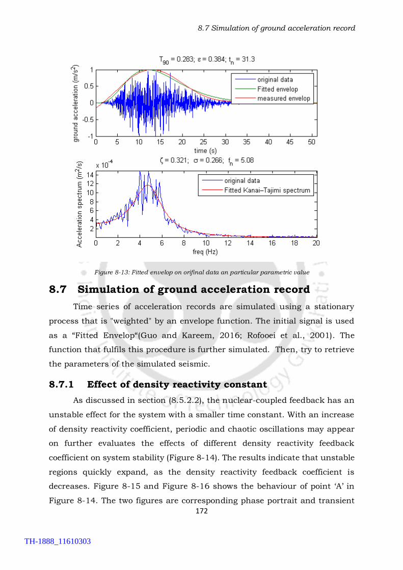
8.7 Simulation of ground acceleration record
172
Figure 8-13: Fitted envelop on orifinal data an particular parametric value
8.7 Simulation of ground acceleration record
Time series of acceleration records are simulated using a stationary
process that is "weighted" by an envelope function. The initial signal is used
as a “Fitted Envelop“(Guo and Kareem, 2016; Rofooei et al., 2001). The
function that fulfils this procedure is further simulated. Then, try to retrieve
the parameters of the simulated seismic.
8.7.1 Effect of density reactivity constant
As discussed in section (8.5.2.2), the nuclear-coupled feedback has an
unstable effect for the system with a smaller time constant. With an increase
of density reactivity coefficient, periodic and chaotic oscillations may appear
on further evaluates the effects of different density reactivity feedback
coefficient on system stability (Figure 8-14). The results indicate that unstable
regions quickly expand, as the density reactivity feedback coefficient is
decreases. Figure 8-15 and Figure 8-16 shows the behaviour of point ‘A’ in
Figure 8-14. The two figures are corresponding phase portrait and transient
TH-1888_11610303

8.7 Simulation of ground acceleration record
173
of two state variables. Similarly, Figure 8-17 and Figure 8-18 are the phase
portrait and transient plot of state variables corresponding to point ‘B’ of
Figure 8-14. A different behaviour of density reactivity coefficient has been
observed here. The system blow-off at the design value of density reactivity
coefficient, but shows the dynamical behaviour of the system at considerable
smaller value of this coefficient.
Figure 8-14: Stability map of Density reactivity constant
Figure 8-15: Phase potrate of GO* and ZPC* corresponding to point “A”
1.5
2.5
7.5 8.5 9.5 10.5
Nsp
c
Ntpc1.00E-02 1.00E-01
A B
0.99
1.00
1.01
1.02
1.03
0.16 0.16 0.16 0.16 0.17 0.17 0.17 0.17 0.17 0.18
Go
*
Zpc*
Stable
Unstable
TH-1888_11610303

8.7 Simulation of ground acceleration record
174
Figure 8-16: Transient of ZPC* corresponding to point “A”
Figure 8-17: Phase potrate of GO* and ZPC* corresponding to point “B”
0.16
0.16
0.17
0.17
0.18
0 2 4 6 8 10 12 14 16
Zp
c*
t*
0.99
1.00
1.01
1.02
1.03
1.04
0.15 0.15 0.16 0.16 0.17 0.17 0.18
Go
*
Zpc*
TH-1888_11610303

8.8 Conclusions
175
Figure 8-18: Transient of ZPC* corresponding to point “B”
8.8 Conclusions
When a nuclear power plant is subjected to a huge earthquake, the seismic
vibration propagates through the core internals and shakes the coolant water
with measurable oscillating acceleration compared with the gravitational one.
Hence, in this work, a preliminary effort is made which is based on the
stability analysis on SCWR due to two different seismic oscillation models;
finally, following observations have been established.
a) LPM is used to study the transient response of the system when
external forcing, in this case seismic wave is applied.
b) LPM is used first time to study Seismic effect on SCWR.
c) Results can be used as a preliminary data for further stability analysis.
d) More realistic modal has been used for stability analysis of SCWR. In
which the real seismic data has been used for the simulations
e) Coupled neutronics and thermal hydraulic stability analysis has been
done.
f) Stability map has been plotted for T-H and neutronics parameters.
g) Most of the thermal hydraulic and neutronics parametric study giver
traditional nature of stability.
0.15
0.15
0.16
0.16
0.17
0.17
0.18
0.00 2.00 4.00 6.00 8.00 10.00
Zp
c*
t*
TH-1888_11610303

8.8 Conclusions
176
h) System with a large density reactivity feedback coefficient in Kanai–
Tajimi model would enhance unstable.
TH-1888_11610303

8.8 Conclusions
177
TH-1888_11610303

9.1 Summary
178
SUMMARY AND CONCLUSIONS
Present thesis work primarily focuses on the analysis of flow instability
in one of the most powerful concepts under the Generation-IV nuclear reactor;
SCWR. The work mainly consists of numerical studies on flow instabilities in
a forced circulation supercritical system. Thermal-hydraulic as well as
coupled neutronics-thermohydraulic instabilities. Linear, Nonlinear
oscillations, and bifurcations have also been investigated. Parametric effects
on the stability, oscillation modes, bifurcation characteristics, in supercritical
forced circulation reactors have been investigated. Furthermore, a
downscaled model is developed to study the complex phenomena in laboratory
conditions; moreover, a scaled method is proposed which is useful for the
study of both the natural as well as the forced circulation system. For further
analysing about the stability of the system, a simple and effective model has
been developed as the Lumped Parameter Model (LPM). Using LPM, a linear
and well nonlinear stability analysis has been done for the various parametric
conditions. Finally, the stability analysis due to the seismic effect on SCWR
has also been considered by using the same LPM.
9.1 Summary
Performing experiment at the lab with supercritical water, particularly
for the stability analysis, is a difficult task, due to the high level of
pressure and temperature involved. That necessitates scaling analysis
for the development of reduced-scale models to simulate true-scale
prototype under lab condition. The study, therefore, attempts to develop
a scaling methodology focused on stability analysis and to identify a
less-restrictive model fluid, while proposing generalized scaling rules
pre-serving the phenomenological physics. US reference design of
SCWR is selected as the prototype. Four characterizing dimensionless
groups are recognized from the non-dimensional conservation
equations un-der imposed pressure boundary condition, while the
TH-1888_11610303

9.1 Summary
179
system pressure for the model fluid is identified noting the region of
similarity on the plane of non-dimensional density and non-
dimensional pressure. Two-zone LPM is used encompassing the
thermal-hydraulic, fuel dynamics and power dynamics equations,
which are subsequently employed for linear stability analysis and
transient simulations. Both approaches produced the same stability
maps, leading to a generalized representation. Several other model
fluids have been studied, such as CO2, Ammonia and R23 and R134a.
Among all R134a is concluded to be the most suitable model fluid from
both power and pressure point of view.
The dynamic characteristics of SCWR is different from existing reactors
due to the supercritical conditions of the coolant. This necessitates the
study of the stability behaviour of SCWR, which requires a dynamic
model of the reactor. A simple unsteady LPM for coupled neutronics-
thermohydraulic transients for SCWR has been developed. The LPM
includes point reactor kinetics for neutron balance and a two-region
model for fuel and coolant thermal hydraulics. The results of dynamic
simulation and linear stability analysis are shown by plotting stability
maps. These results show good agreement with each other.
Furthermore, to study the effect of parameters on the stability of the
system, variations of some geometric, control and neutronics
parameters are analyzed. The stability maps predicted by the LPM are
also compared with those obtained with RELAP5 code and are found to
show similar trends.
It is very difficult to study the stability of a complex system such as
SCWR by linear stability analysis. It is valid for local stability analysis;
nonlinear stability analysis is essential for the global stability analysis.
Therefore, a simple unsteady LPM for SCWR has been used. It includes
point reactor kinetics for neutron balance and a two-region model for
fuel and coolant thermal hydraulics. Regions of stable and unstable
operation are identified in the parameter space by linear stability
analysis. Bifurcation analysis is carried out to capture the non-linear
TH-1888_11610303

9.1 Summary
180
dynamics of the system. Generalized Hopf (GH) points are, and
parameter ranges for supercritical (soft and safe), and subcritical (hard
and dangerous) Hopf bifurcations are identified. The type of transient
behavior of the system for finite (though small) perturbations are
predicted based on this analysis. The existence of predicted limit cycles
is confirmed by numerical simulation of the nonlinear ODEs, using the
shooting technique in case of unstable limit cycles. Furthermore, the
effects of geometric, control and neutronics parameters on the stability
of the system are studied.
To know the extents of stability margin by increasing the numbers of
nodes, the study has been done using the three-zone model. An
improvement on that in the form of a three-region model is proposed,
which was found to provide a similar prediction on the stability
prediction of SCWR. Therefore, present study carries out a lumped
parameter base stability analysis for a heated channel with
supercritical fluid following three-region model. In the current model
stability analysis has been done on three geometrical parameters and
their detailed stability map has been plotted for locating the stable and
unstable zones.
In this study, two types of seismic model have been analysed. The
vertical seismic oscillations motion is taken into consideration. The
simple sinusoidal model to simulate the artificial ground wave, an
another more realistic earthquake model which is Kanai-Tajimi model
has been used to see the more realistic analysis of SCWR. The vertical
seismic acceleration was simply represented by one sine curve, and the
effects of the frequency and amplitude of the sine wave and the degree
of instability of the initial state, which is dependent on the power-to-
flow ratio at the core, the axial power distribution and so forth, were
investigated. This paper describes the methods and models applied and
the major calculated results obtained. The primary objective of this
study is to supply quantitative information useful for determining the
significant effects of seismic wave on SCWR system. In order to meet
TH-1888_11610303

9.2 Conclusions
181
the objective, the transient thermal hydraulic in-house code is used
after modified to take into account external acceleration in addition to
gravity.
9.2 Conclusions
As summarized in the preceding section, a detailed investigation of
parametric effects on the stability, scaling methodology and nonlinear
oscillation in supercritical systems has been presented in this work. Based on
these results the following conclusions can be drawn
A new scaling approach proposed exclusively for SCWRs.
Four different fluids are compared by equating the important
dimensionless groups.
R134a is found to be the most suitable scaling fluid from temperature,
pressure and power point of view. It also leads to more compact design
and poses convenient chemical properties.
Stability behavior of the prototype with water and model with R134a is
compared using both linear stability analysis and transient
simulations. Both approaches are found to produce identical results.
System pressure is found to have insignificant role from stability point
of view. RELAP5 is employed for validation of the developed model and
the present lumped approach is observed to produce conservative
estimate of the stability threshold.
Parametric effects on the stability threshold have been investigated and
major conclusions are given below. A reduced-order model, also called
lumped parameter model (LPM), is proposed in the present study to
ascertain the stability characteristics of SCWR.
Increasing the heated channel length has destabilizing effect on
the system, which is quite common in boiling channels also.
Stabilizing effect on the system has been observed by increasing
the hydraulic diameter.
Increase in inlet orifice coefficient has stabilizing effect whereas
the reverse can be observed for the outlet orifice.
TH-1888_11610303

9.3 Future works
182
System pressure is found to have negligible effect on the non-
dimensional stability threshold.
The stability of the reactor decreases with increase in fuel time
constant.
The stability of the reactor is found to increase with an increase
in negative enthalpy reactivity coefficient.
Parametric trends in 3-zone model for heated channel length, hydraulic
diameter and orifice coefficients are similar to 2-zone model and the
difference in the MSB is 2-8%, therefore, 2-zone model is more suitable
for further study.
Linear as well non-linear stability analysis of SCWR has been carried
out by employing a LPM, considering thermal hydraulics as well as
neutronics of the system. Based on the study, major findings are the
following.
Generalized Hopf (GH) bifurcation is observed from non-linear
analysis of the system.
The range of unstable limit cycle is obtained by predicting its
boundary through the shooting technique.
The stability of the reactor deteriorates with increase in fuel time
constant.
The stability of the reactor is found to improve marginally with
increase in density reactivity coefficient.
Increasing the heated channel length and area ratio has
destabilizing effect on the system, which is quite common in
boiling channels also.
Reduction in the mass flow rate has destabilizing effect on SCWR,
similar to BWR and CANDU SCWR.
9.3 Future works
Although a lots of work have been carried out by different researchers in
different field of SCWR, but still a lot of effort can be done in this field for
TH-1888_11610303
9.3 Future works
183
improvement. Few of the observations and suggestions, which may be useful
in future extensions of the present work, is given below.
1. This thesis presents a detailed analysis of instabilities and scaling in
forced circulation systems. The knowledge generated by this study is
likely to be useful for the design and operation of SCWR for further
study. Based on these studies, a suitable combination of geometrical,
feedback, and neutronics parameters can be designed.
2. Scaling method, a unified model can be made for both natural
circulation (NC) and forced circulation (FC) system. SCWR safety
including power at start-up and during set-down.
3. Start-up transients need to be investigated using nonlinear dynamics
methods. Extensive research has been done on linear analysis of
instabilities in natural circulation, there is a scope for nonlinear
analysis of instabilities using the techniques of nonlinear dynamics and
bifurcation theory.
4. The knowledge gained from nonlinear analysis can be used for
designing better control systems and safety measures. Study of
transient behaviour of SCW and scaled fluid at SC pressure. Unified
stability map covering the entire parameter space and all types of
instabilities.
5. Many numerical codes have been developed to simulate neutronics and
thermal hydraulics, but development of user-friendly software with
graphic user interface remains to be done. This will facilitate extensive
numerical simulations of instabilities and thus help in improving
reactor safety.
6. In the present study a high pressure lumped parameter model is used.
The fluid properties are evaluated at constant system pressure. This
restricts the use of this model to high pressure conditions and
operational transients. In order to investigate the nonlinear dynamics
TH-1888_11610303

9.3 Future works
184
of start-up-transients, a lumped parameter model in which fluid
properties are evaluated at local pressure is to be used. This needs a
further study.
7. Nonlinear dynamic analysis of the SCWR using MATLAB tools and
Shooting method. Using these stable and unstable limit cycle has been
predicated. More detailed analysis can be possible by using some
advance nonlinear codes.
TH-1888_11610303

9.3 Future works
185
TH-1888_11610303

0 Journals
186
LIST OF PUBLICATIONS
Journals
1. Shankar, D., Basu, D.N., Pandey, M., 2017. Development and Analysis of a
Novel Scaling Methodology for Stability Appraisal of Supercritical Flow
Channels. Nucl. Eng. Des. 323, 46–55
2. Shankar, D., Pandey, M., Basu, D.N., 2018. Parametric Effects on Coupled
Neutronic Thermohydraulic Stability Characteristics of Supercritical Water
Cooled Reactor. Ann. Nucl. Energy 112, 120–131
3. Shankar, D., Pandey, M. & Basu, D.N., 2017. Nonlinear analysis of nuclear
coupled density wave instability in time domain for SCWR. Ann. Nucl. Energy
(Under Revision).
4. Shankar, D., Basu, D.N., Pandey, M., 2017. Neutron-Coupled Thermal
Hydraulic Calculation of SCWR Under Seismic Wave Acceleration. Nucl. Eng.
Des. (Under Preparations)
Conferences
1. Shankar, D., Basu, D. N., Pandey, M., Study on Design of Scaled Down Test
Facilities for Investigation of Instabilities in Supercritical Water Reactor.
ICONE21-16638, In: Proceedings of 16th International conference on Nuclear
Engineering ICONE-21, Chengdu, China, July 29-Aug 2, 2013.
2. Shankar, D., Basu, D. N., Pandey, M., Lumped Parameter Analysis for A
Supercritical Water Cooled Reactor Following Three-Region Model,
IHMTC2017-13-0950, Proceedings of the 24th National and 2nd International
ISHMT-ASTFE, Heat and Mass Transfer Conference (IHMTC-2017), December
27-30, 2017, BITS Pilani, Hyderabad, India.
3. Shankar, D., Pandey, M., Basu, D. N., Coupled-Neutronic-Thermalhydraulic
Stability Appraisal of Supercritical Forced Flow Channels Following Lumped
Parameter Approach, Proceedings of the 16th International Heat Transfer
Conference (IHTC16-23961), IHTC-16, August 10-15, 2018, Beijing, China
TH-1888_11610303

0 Conferences
187
TH-1888_11610303

188
APPENDIX-A
Flow chart of stability analysis of SCWR
If 𝑎𝑙𝑙 ȁ𝑅𝑒(𝜆)ȁ < 10−6
Start
Initial Condition (Steady state): 𝑍𝑃𝐶 ,ℎ𝑜 , 𝑇𝑓 , 𝑃𝑜,𝐶𝑜
If
∆𝑝 = ∆𝑝𝑐𝑎𝑙
Calculate: ∆𝑝𝑐𝑎𝑙
Inlet Condition: Give Inlet Temperature
Give System Power
Define: ∆𝑝
NO
YES
End
Jacobian Matrix: 𝑍𝑃𝐶 ,ℎ𝑜 , 𝑇𝑓 ,𝑃𝑜,𝐶𝑜
Eigenvalue of Jacobian Matrix
YES
NO
Guess Mass flow rate
TH-1888_11610303

189
TH-1888_11610303

190
REFERENCES
Abram, T., Ion, S., 2008. Generation-IV nuclear power: A review of the state
of the science. Energy Policy 36, 4323–4330. https://doi.org/10.1016/j.e
pol.2008.09.059
Ambrosini, W., 2008. Lesson learned from the adoption of numerical tec
niques in the analysis of nuclear reactor thermal-hydraulic phenomena.
Prog. Nucl. Energy 50, 866–876.
https://doi.org/10.1016/j.pnucene.2008.02.008
Ambrosini, W., Ferreri, J.C., 2006. Analysis of basic phenomena in boiling
channel instabilities with different flow models and numerical schemes. In:
14th International national Conference on Nuclear Engineering (ICONE 14),
Miami, Florida, USA, July 17–20.
Ambrosini, W., Sharabi, M., 2008. Dimensionless parameters in stability
analysis of heated channels with fluids at supercritical pressures. Nucl.
Eng. Des. 238, 1917–1929.
https://doi.org/10.1016/j.nucengdes.2007.09.008
Ambrosini, W., Di Marco, P. and Ferreri, J. C., 2000. Linear and nonlinear
analysis of density-wave instability phenomena. Heat and Technology,
18(1), pp. 27–36.
Ampomah-amoako, E., Akaho, E.H.K., Nyarko, B.J.B., Ambrosini, W., 2013.
Annals of Nuclear Energy CFD analysis of the dynamic behaviour of a fuel
rod subchannel in a supercritical water reactor with point kinetics. Ann.
Nucl. Energy 59, 211–223.
https://doi.org/10.1016/j.anucene.2013.04.008
TH-1888_11610303

191
Anishchenko, V.S., Vadivasova, T.E., Strelkova, G.I., 2014. Deterministic
Nonlinear Systems. https://doi.org/10.1007/978-3-319-06871-8
Barragán-Martínez, A.M., Martin-Del-Campo, C., François, J.L., Espinosa-
Paredes, G., 2013. MCNPX and HELIOS-2 comparison for the neutronics
calculations of a Supercritical Water Reactor HPLWR. Ann. Nucl. Energy 51,
181–188. https://doi.org/10.1016/j.anucene.2012.08.013
Blázquez, J., Montalvo, C., García-berrocal, A., Balbás, M., 2013. Annals of
Nuclear Energy Searching the beginning of BWR power instability events
with the Hilbert Huang transform. Ann. Nucl. Energy 54, 281–288.
https://doi.org/10.1016/j.anucene.2012.09.005
Boure, J.A., Bergles, A.E., Tong, L.S., 1973. Review of two-phase flow insta-
bility. Nucl. Eng. Des. 25, 165–192. https://doi.org/10.1016/0029-
5493(73)90043-5
Cai, J., Ishiwatari, Y., Ikejiri, S., Oka, Y., 2009. Thermal and stability con-
siderations for a supercritical water-cooled fast reactor with downward-flow
channels during power-raising phase of plant startup. 239, 665–679.
https://doi.org/10.1016/j.nucengdes.2008.12.010
Chatoorgoon, V., 2001. Stability of supercritical fluid flow in a single-
channel natural-convection loop. Int. J. Heat Mass Transf. 44, 1963–1972.
https://doi.org/10.1016/S0017-9310(00)00218-0
Chaudri, K.S., Tian, W., Su, Y., Zhao, H., Zhu, D., Su, G., Qiu, S., 2013.
Coupled analysis for new fuel design using and UC for SCWR. Prog. Nucl.
Energy 63, 57–65. https://doi.org/10.1016/j.pnucene.2012.11.001
TH-1888_11610303

192
Cheng, X., Schulenberg, T., 2001. Heat Transfer at Supercritical Pressures
- Literature Review and Application to an HPLWR.
Commonwealth Edison Co., 1988. Reactor scram on high average power
monitor flux level due to the personal valvingerror, LER 88-003-00.
Colombo, M., Cammi, A., Papini, D., Ricotti, M.E., 2012. RELAP5/MOD3.3
study on density wave instabilities in single channel and two parallel chan-
nels. Prog. Nucl. Energy 56, 15–23.
https://doi.org/10.1016/j.pnucene.2011.12.002
Debrah, S.K., Ambrosini, W., Chen, Y., 2013. Discussion on the stability of
natural circulation loops with supercritical pressure fluids. Ann. Nucl.
Energy 54, 47–57. https://doi.org/10.1016/j.anucene.2012.10.015
Dhooge, a., Govaerts, W., Kuznetsov, Y. a., 2003. MATCONT: A MATLAB
package for numerical bifurcation analysis of ODEs. ACM Trans. Math.
Softw. 29, 141–164. https://doi.org/10.1145/779359.779362
Dutta, G., Maitri, R., Zhang, C., Jiang, J., 2015a. Numerical models to pre-
dict steady and unsteady thermal-hydraulic behaviour of supercritical
water flow in circular tubes Atomic Energy of Canada Limited. Nucl. Eng.
Des. 289, 155–165. https://doi.org/10.1016/j.nucengdes.2015.04.028
Dutta, G., Zhang, C., Jiang, J., 2015b. Analysis of flow induced density
wave oscillations in the CANDU supercritical water reactor. Ann. Nucl.
Energy 83, 264–273. https://doi.org/10.1016/j.anucene.2015.04.023
Durga Prasad, G.V., Pandey, M., 2008. Stability analysis and nonlinear
dynamics of natural circulation boiling water reactors. Nucl. Eng. Des. 238,
229–240. https://doi.org/10.1016/j.nucengdes.2007.05.004
TH-1888_11610303
193
Dykin, V., Demazière, C., Lange, C., Hennig, D., 2013. Annals of Nuclear
Energy Investigation of local BWR instabilities with a four heated-channel
Reduced Order Model. Ann. Nucl. Energy 53, 320–330.
https://doi.org/10.1016/j.anucene.2012.07.022
E. Gialdi, S. Grifoni, C. Parmeggiani and C. Tricoli, 1985. Core stability in
operating BWR: operating experience. Prog. Nucl. Energy, 15, 447-459.
Fu, S.W., Liu, X.J., Zhou, C., Xu, Z.H., Yang, Y.H., Cheng, X., 2012. Annals
of Nuclear Energy Modification and application of the system analysis code
ATHLET to trans-critical simulations. 44, 40–49.
https://doi.org/10.1016/j.anucene.2012.02.005
Gajev, I., Ma, W., Kozlowski, T., 2013. Annals of Nuclear Energy Space –
time convergence analysis on BWR stability using TRACE / PARCS. Ann.
Nucl. Energy 51, 295–306.
https://doi.org/10.1016/j.anucene.2012.08.018
Guo, Y., Kareem, A., 2016. System identification through nonstationary
data using Time – Frequency Blind Source Separation. J. Sound Vib. 371,
110–131. https://doi.org/10.1016/j.jsv.2016.02.011
Guido, G., Converti, J. and Clausse, A., 1991. Density-wave oscillations in
paraUel channels - an analytical approach. Pb hb’, 125, pp. 121–136.
Henry, A.F., 1975. Nuclear Reactor Analysis. MIT, Cambridge. International
Atomic Energy Agency, 1999. Basic Safety Principles for Nuclear Power
Plants 1. INSAG 12. IAEA.
TH-1888_11610303

194
Hirano, M., Tamakoshi, T., 1996. An analytical study on excitation of nucle-
ar coupled thermal hydraulic instability due to seismically induced reso-
nance in BWR. Nucl. Eng. Des. 162, 307–315.
https://doi.org/10.1016/0029-5493(95)01128-5
Hou, D., Lin, M., Liu, P., Yang, Y., 2011. Stability analysis of parallel-
channel systems with forced flows under supercritical pressure. Ann. Nucl.
Energy 38, 2386–2396. https://doi.org/10.1016/j.anucene.2011.07.021
Hou, X., Sun, Z., Fan, G., Wang, L., 2017. Experimental and analytical
investigation on the flow characteristics in an open natural circulation
system. Appl. Therm. Eng. 124, 673–687.
https://doi.org/10.1016/j.applthermaleng.2017.05.201
Ikejiri, S., Ishiwatari, Y., Oka, Y., 2010. Safety analysis of a supercritical-
pressure water-cooled fast reactor under supercritical pressure. Nucl. Eng.
Des. 240, 1218–1228. https://doi.org/10.1016/j.nucengdes.2009.12.034
Ishii, M., 1971. Thermally induced flow instabilities in two-phase mixtures
in thermal equilibrium. PhD. Georg. Inst. Technol.
Ishiwatari, Y., Oka, Y., Koshizuka, S., 2003. Control of a High Temperature
Supercritical Pressure Light Water Cooled and Moderated Reactor with
Water Rods. J. Nucl. Sci. Technol. 40, 298–306.
https://doi.org/10.1080/18811248.2003.9715359
J.C. Shaug, J.T. Tatsumi, J.G.M. 1987. Analysis of fluid dynamics in a
boiling water reactor in a varying acceleration field, Forum on Unsteady
Fluid Flow. ASME Winter Annual Meeting, Boston, USA, October.
TH-1888_11610303

195
Jäger, W., Sánchez Espinoza, V.H., Hurtado, A., 2011. Review and proposal
for heat transfer predictions at supercritical water conditions using existing
correlations and experiments. Nucl. Eng. Des. 241, 2184–2203.
https://doi.org/10.1016/j.nucengdes.2011.03.022
Jackson, J.D., Hall, W.B., 1979. Influence of Buoyancy on Heat Transfer to
Fluids in Vertical Tubes under Turbulent Conditions, Turbulent Forced
Convection in Channels and Bundles. Hemishpere, New York, pp. 613–640.
Jain, R., 2005. Thermal-hydraulic instabilities in natural circulation flow
loops under supercritical conditions. PhD thesis, University of Wisconsin-
Madison.
Jain, V., Nayak, A.K., Vijayan, P.K., Saha, D., Sinha, R.K., 2010.
Experimental investigation on the flow instability behavior of a multi-
channel boiling natural circulation loop at low-pressures. Exp. Therm. Fluid
Sci. 34, 776–787. https://doi.org/10.1016/j.expthermflusci.2010.01.007
Jain, P.K., Rizwan-uddin, 2008. Numerical analysis of supercritical flow
instabilities in a natural circulation loop. Nucl. Eng. Des. 238, 1947–1957.
https://doi.org/10.1016/j.nucengdes.2007.10.034
Joen, C.T., Gilli, L., Rohde, M., T’Joen, C., Gilli, L., Rohde, M., Joen, C.T.,
Gilli, L., Rohde, M., 2011. Sensitivity analysis of numerically determined
linear stability boundaries of a supercritical heated channel. Nucl. Eng. Des.
241, 3879–3889. https://doi.org/10.1016/j.nucengdes.2011.07.005
K. Fukuda and T. Kobori., 1979. Classification of two-phase flow
instabilities by density-wave oscillation model. J. Nucl. Sci. Technol. 16(2),
95, 18.
TH-1888_11610303

196
Kakac, S., Bon, B., 2008. A Review of two-phase flow dynamic instabilities
in tube boiling systems. Int. J. Heat Mass Transf. 51, 399–433.
https://doi.org/10.1016/j.ijheatmasstransfer.2007.09.026
Khabensky, V., Gerliga, V., 2012. Coolant Flow Instabilities in Power
Equipment. https://doi.org/10.1201/b13658
Kiss, A., Balaskó, M., Horváth, L., Kis, Z., Aszódi, A., 2017. Experimental
investigation of the thermal hydraulics of supercritical water under natural
circulation in a closed loop. Ann. Nucl. Energy 100, 178–203.
https://doi.org/10.1016/j.anucene.2016.09.020
Kotlyar, D., Shaposhnik, Y., Fridman, E., Shwageraus, E., 2011. Coupled
neutronics thermo-hydraulic analysis of full PWR core with Monte-Carlo
based BGCore system. Nucl. Eng. Des. 241, 3777–3786.
https://doi.org/10.1016/j.nucengdes.2011.07.028
Kozmenkov, Y., Rohde, U., Manera, A., 2012. Validation of the RELAP5 code
for the modeling of flashing-induced instabilities under natural-circulation
conditions using experimental data from the CIRCUS test facility. Nucl. Eng.
Des. 243, 168–175. https://doi.org/10.1016/j.nucengdes.2011.10.053
Kurganov, V.A., Zeigarnik, Y.A., Maslakova, I. V, 2012. Heat transfer and
hydraulic resistance of super-critical-pressure coolants. Part I : Specifics of
thermophysical properties of supercritical pressure fluids and turbulent
heat transfer under heating con-ditio. Int. J. Heat Mass Transf. 55, 3061–
3075. https://doi.org/10.1016/j.ijheatmasstransfer.2012.01.031
Lahey, R.T., 1986. Advance in the Analytical Modeling of Linear and
Nonlinear Density-Wave Instability Modes. Nucl. Eng. Des. 95, 5–34.
TH-1888_11610303

197
Lee, J. Der, Pan, C., 2005. Nonlinear analysis for a nuclear-coupled two-
phase natural circulation loop. Nucl. Eng. Des. 235, 613–626.
https://doi.org/10.1016/j.nucengdes.2004.09.008
Lewins, J., 1961. Nuclear reactor kinetics and control.
https://doi.org/10.1007/978-4-431-54195-0
Li, H. bo, Zhao, M., Hu, Z. xiao, Zhang, Y., Wang, F., 2018. Experimental
study of supercritical water heat transfer deteriorations in different
channels. Ann. Nucl. Energy 119, 240–256.
https://doi.org/10.1016/j.anucene.2018.05.009
Li, S., Chatoorgoon, V., Ormiston, S.J., 2018. Numerical study of oscillatory
flow instability in upward flow of supercritical water in two heated parallel
channels. Int. J. Heat Mass Transf. 116, 16–29.
https://doi.org/10.1016/j.ijheatmasstransfer.2017.08.115
Licht, J., 2009. Heat Transfer and Fluid Flow Characteristics in
Supercritical 131, 1–14. https://doi.org/10.1115/1.3090817
Manera, A., Zboray, R., Van Der Hagen, T.H.J.J., 2003. Assessment of linear
and non-linear auto-regressive methods for BWR stability monitoring. Prog.
Nucl. Energy 43, 321–327. https://doi.org/10.1016/S0149-1970
(03)00005-2
Marcel, C.P., Rohde, M., Masson, V.P., Hagen, T.H.J.J. Van Der, 2009.
Fluid-to-fluid modeling of supercritical water loops for stability analysis. Int.
J. Heat Mass Transf. 52, 5046–5054.
https://doi.org/10.1016/j.ijheatmasstransfer.2009.03.022
TH-1888_11610303

198
March-Leuba, J., Rey, J., 1993. Coupled thermohydraulic-neutronics
instabilities in boiling water nuclear reactors: a review of the state of the
art. Nucl. Eng. Des. 145, 97–111. https://doi.org/10.1016/0029-
5493(93)90061-D
Mcevoy, E., 2009. Using Matlab to integrate Ordinary Differential Equations
(ODEs) 45, 1–9.
Meijer, H., 2008. Matcont Tutorial : ODE GUI version Getting started /
Installation 14, 1–9.
Meloni, P., Polidori, M., 2007. A neutronics -thermalhydraulics model for
preliminary studies on TRADE dynamics 237, 1704–1717.
https://doi.org/10.1016/j.nucengdes.2007.03.014
Merroun, O., Almers, A., Bardouni, T. El, Bakkari, B. El, Chakir, E., 2009.
Analytical benchmarks for verification of thermal-hydraulic codes based on
sub-channel approach 239, 735–748.
https://doi.org/10.1016/j.nucengdes.2009.01.005
Mishra, A.M., Singh, S., 2016. Non linear stability analysis of parallel
channels with natural circulation. Nucl. Eng. Des. 309, 136–150.
https://doi.org/10.1016/j.nucengdes.2016.09.002
Monti, L., Starflinger, J., Schulenberg, T., 2011. Development of a coupled
neutronic-thermal-hydraulic tool with multi-scale capabilities and
applications to HPLWR core analysis. Nucl. Eng. Des. 241, 1579–1591.
https://doi.org/10.1016/j.nucengdes.2011.02.012
TH-1888_11610303

199
Mousavian, S.K., Misale, M., D’Auria, F., Salehi, M.A., 2004. Transient and
stability analysis in single-phase natural circulation. Ann. Nucl. Energy 31,
1177–1198. https://doi.org/10.1016/j.anucene.2004.01.005
G.A. Murphy, 1988. Selected safety-related events, Nucl. Safety, 29
(3), 356-362
Nakatsuka, T., Oka, Y., Koshizuka, S., 1998. Control of a fast reactor cooled
by super- critical light water. Nuclear Technology 121 (1), 81–92.
Nayak, A.K., Vijayan, P.K., Saha, D., Raj, V.V., 2000. Analytical study of nu-
clear-coupled density-wave instability in a natural circulation pressure tube
type boiling water reactor. Nucl. Eng. Des. 195, 27–44.
Nayfeh AH, Balachandran B., 1992. Cyclic motions near a Hopf bifurcation
of a four-dimensional system. Nonlinear Dyn. 1, 19–39.
Ortega, T.G., Class, A., Jr, R.T.L., Schulenberg, T., 2008. Stability analysis
of a uniformly heated channel with super-critical water. Nucl. Eng. Des.
238, 1930–1939. https://doi.org/10.1016/j.nucengdes.2007.10.031
Pandey, M., 1996. Nonlinear Reactivity Interactions in Fission Reactor
Dynamical Systems. Ph.D. Thesis, Indian Institute of Technology, Kanpur.
Pandey, M., Kumar, C.N., 2007. Lumped parameter modeling and stability
analysis of supercritical water-cooled reactor. In the 12th International
Topical Meeting on Nuclear Reactor Thermal Hydraulics (NURETH-12)
Sheraton Station Square, Pittsburgh, Pennsylvania, U.S.A. pp. 1–11.
TH-1888_11610303

200
Pandey, V., Singh, S., 2016. A bifurcation analysis of boiling water reactor
on large domain of parametric spaces. Commun. Nonlinear Sci. Numer.
Simul. 38, 30–44. https://doi.org/10.1016/j.cnsns.2016.01.018
Paruya, S., Maiti, S., Karmakar, A., Gupta, P., Sarkar, J.P., 2012. Lumped
parameterization of boiling channel — Bifurcations during density wave
oscillations. Chem. Eng. Sci. 74, 310–326.
https://doi.org/10.1016/j.ces.2012.02.039
Papini, D., Cammi, A., Colombo, M., Ricotti, M.E., 2012. Time-domain li ear
and non-linear studies on density wave oscillations. Chem. Eng. Sci. 81,
118–139. https://doi.org/10.1016/j.ces.2012.06.005
Paul, S., Singh, S., 2014. Analysis of sub- and supercritical Hopf bifurcation
with a reduced order model in natural circulation loop. Int. J. Heat Mass
Transf. 77, 344–358.
https://doi.org/10.1016/j.ijheatmasstransfer.2014.05.033
Peng, S.J., Podowski, M.Z., Lahey, R.T., 1986. BWR linear stability analysis.
Nucl. Eng. Des. 93, 25–37. https://doi.org/10.1016/0029-5493(86)90192-
5
Pioro, I.L., Duffey, R.B., 2005. Experimental heat transfer in supercritical
water flowing inside channels (survey) 235, 2407–2430.
https://doi.org/10.1016/j.nucengdes.2005.05.034
Prasad, G.V.D., Pandey, M., Kalra, M.S., 2007. Review of research on flow
instabilities in natural circulation boiling systems. Prog. Nucl. Energy 49.
https://doi.org/10.1016/j.pnucene.2007.06.002
TH-1888_11610303

201
Pucciarelli, A., Ambrosini, W., 2016. Fluid-to-fluid scaling of heat transfer
phenomena with supercritical pressure fluids: Results from RANS analyses.
Ann. Nucl. Energy 92, 21–35.
https://doi.org/10.1016/j.anucene.2016.01.028
Rao, Y.F., Fukuda, K., Kaneshima, R., 1995. Nuclear Engineering and
Design Analytical study of coupled neutronic and thermodynamic
instabilities in a boiling channel 133–144.
Regis, C.R., Cotta, R.M., Su, J., 2000. Improved lumped analysis of
transient heat conduction in a nuclear fuel rod. Int. Commun. Heat Mass
Transf. 27, 357–366. https://doi.org/10.1016/S0735-1933(00)00116-0
Reiss, T., Fehér, S., Czifrus, S., 2008. Coupled neutronics and
thermohydraulics calculations with burn-up for HPLWRs. Prog. Nucl.
Energy 50, 52–61. https://doi.org/10.1016/j.pnucene.2007.12.002
Roberto, T.D., Silva, M.A.B. Da, Lapa, C.M.F., 2016. Development of a test
facility for analyzing transients in supercritical water-cooled reactors by
fractional scaling analysis. Nucl. Eng. Des. 296, 9–18.
https://doi.org/10.1016/j.nucengdes.2015.10.025
Rofooei, F.R., Mobarake, A., Ahmadi, G., 2001. Generation of artificial
earthquake records with a nonstationary Kanai-Tajimi model. Eng. Struct.
23, 827–837. https://doi.org/10.1016/S0141-0296(00)00093-6
Rohde, M., Marcel, C.P., T’Joen, C., Class, A.G., Van Der Hagen, T.H.J.J.,
2011. Downscaling a supercritical water loop for experimental studies on
system stability. Int. J. Heat Mass Transf. 54, 65–74.
https://doi.org/10.1016/j.ijheatmasstransfer.2010.09.063
TH-1888_11610303

202
Roy, R.P., Jain, P., Kalra, S.P., 1988. Dynamic instability experiments in a
boiling flow system. Int. J. Heat Mass Transf. 31, 1947–1952.
https://doi.org/10.1016/0017-9310 (88)90209-8
Rohde, M., Marcel, C.P., T’Joen, C., Class, A.G., Van Der Hagen, T.H.J.J.,
2011. Downscaling a supercritical water loop for experimental studies on
system stability. Int. J. Heat Mass Transf. 54, 65–74.
https://doi.org/10.1016/j.ijheatmasstransfer.2010.09.063
Ruspini, L.C., Marcel, C.P., Clausse, A., 2014. Two-phase flow instabilities:
A review. Int. J. Heat Mass Transf. 71, 521–548.
https://doi.org/10.1016/j.ijheatmasstransfer.2013.12.047
Saha, P., Ishii, M., Zuber, N., 1975. Experimental Investigation of The
Thermally Induced Flow Oscillations. In Two-Phase Systems. Am. Soc.
Mech. Eng. 8.
Satou, A., Watanabe, T., Maruyama, Y., Nakamura, H., 2011. Neutron-
Coupled Thermal Hydraulic Calculation of BWR under Seismic Acceleration
2, 120–124.
Schmitt, T., Rodriguez, J., Leyva, I.A., Candel, S., 2012. Experiments and
numerical simulation of mixing under supercritical conditions. Phys. Fluids
24. https://doi.org/10.1063/1.3701374
Schmidt, E., Eckert, E., Grigull, U., 1946. Heat Transfer by Liquids near the
Critical State. Wright Field, Air Materiel Command.
Schulenberg, T., Leung, L.K.H., Oka, Y., 2014. Review of R&D for
supercritical water-cooled reactors. Prog. Nucl. Energy 77, 282–299.
https://doi.org/10.1016/j.pnucene.2014.02.021
TH-1888_11610303

203
Shan, J., Zhang, B., Li, C., Leung, L.K.H., 2009. SCWR subchannel code
ATHAS development and CANDU-SCWR analysis. Nucl. Eng. Des. 239,
1979–1987. https://doi.org/10.1016/j.nucengdes.2009.05.008
Shampine, L.F. and Reichelt, M.W., 1997. The MATLAB ODE suit. SIAM J.
Sci. Compt. 18, 1, 1-22.
Shang, Z., Lo, S., 2010. Numerical investigation of supercritical water-
cooled nuclear reactor in horizontal rod bundles. Nucl. Eng. Des. 240, 776–
782. https://doi.org/10.1016/j.nucengdes.2009.10.029
Sharabi, M., Ambrosini, W., 2009. Discussion of heat transfer phenomena
in fluids at supercritical pressure with the aid of CFD models. Ann. Nucl.
Energy 36, 60–71. https://doi.org/10.1016/j.anucene.2008.10.006
Sharabi, M., Ambrosini, W., He, S., Jackson, J.D., 2008. Prediction of
turbulent convective heat transfer to a fluid at supercritical pressure in
square and triangular channels. Ann. Nucl. Energy 35, 993–1005.
https://doi.org/10.1016/j.anucene.2007.11.006
Sharma, M., Pilkhwal, D.S., Vijayan, P.K., Saha, D., Sinha, R.K., 2010.
Steady state and linear stability analysis of a supercritical water natural cir-
culation loop. Nucl. Eng. Des. 240, 588–597.
https://doi.org/10.1016/j.nucengdes.2009.10.0
Sharma, M., Vijayan, P.K., Pilkhwal, D.S., Asako, Y., 2013. Steady state and
stability characteristics of natural circulation loops operating with carbon
dioxide at supercritical pressures for open and closed loop boundary condi-
tions. Nucl. Eng. Des. 265, 737–754.
https://doi.org/10.1016/j.nucengdes.2013.07.023
TH-1888_11610303

204
Shen, Z., Yang, D., Wang, S., Wang, W., Li, Y., 2017. Experimental and
numerical analysis of heat transfer to water at supercritical pressures. Int.
J. Heat Mass Transf. 108, 1676–1688.
https://doi.org/10.1016/j.ijheatmasstransfer.2016.12.081
Shi, S., Lin, Y., Yang, W.S., 2015. Experimental Stability Maps for a BWR-
type Small Modular Reactor. NURETH-16, Chicago 5498–5511.
Shitsi, E., Debrah, S. K., Agbodemegbe, V. Y. and Ampomah-Amoako, E.
2018. Effect of axial power distribution on flow instability in parallel
channels with water at supercritical pressures. Annals of Nuclear Energy.
Elsevier Ltd, 112, pp. 109–119. doi: 10.1016/j.anucene.2017.10.003
Su, Y., Feng, J., Zhao, H., Tian, W., Su, G., Qiu, S., 2013. Theoretical study
on the fl ow instability of supercritical water in the parallel channels. Prog.
Nucl. Energy 68, 169–176.
https://doi.org/10.1016/j.pnucene.2013.06.005
Suárez, L.E., Montejo, L.A., 2005. Generation of artificial earthquakes via
the wavelet transform. In International Journal of Solids and Structures.
pp. 5905–5919. https://doi.org/10.1016/j.ijsolstr.2005.03.025
Sun, P., Jiang, J. and Shan, J. 2011. Construction of dynamic model of
CANDU-SCWR using moving boundary method. Nuclear Engineering and
Design. Elsevier B.V., 241(5), pp. 1701–1714. doi:
10.1016/j.nucengdes.2011.02.017.
Swapnalee, B.T., Vijayan, P.K., Sharma, M., Pilkhwal, D.S., 2012. Steady
state flow and static instability of supercritical natural circulation loops.
TH-1888_11610303

205
Nucl. Eng. Des. 245, 99–112.
https://doi.org/10.1016/j.nucengdes.2012.01.002
Parker, T.S., Chua, L.O., 1989. Practical Numerical Algorithms for Chaotic
Systems. Springer-Verlag.
T. Ishida and I. Tomiai, 1992. Development of an analysis code for thermal
hydrodynamics of marine reactor under multi-dimensional ship motions,
Proc. 5th Int. Topical Meeting on Reactor Thermal Hydraulics, NURETH-5,
Salt Lake City, USA.
Tian, X., Tian, W., Zhu, D., Qiu, S., Su, G., Xia, B., 2012. Annals of Nuclear
Energy Flow instability analysis of supercritical water-cooled reactor
CSR1000 based on frequency domain. Ann. Nucl. Energy 49, 70–80.
https://doi.org/10.1016/j.anucene.2012.06.023
T’Joen, C., Rohde, M., 2012. Experimental study of the coupled thermo-
hydraulic-neutronics stability of a natural circulation HPLWR. Nucl. Eng.
Des. 242, 221–232. https://doi.org/10.1016/j.nucengdes.2011.10.055
Theler, G. G. and Bonetto, F. J., 2010. On the stability of the point reactor
kinetics equations. Nuclear Engineering and Design, 240(6), pp. 1443–
1449. doi: 10.1016/j.nucengdes.2010.03.007.
Todreas, E, N. and Kazimi, M. S. (2001) Nuclear Systems II: Elements of
Thermal Hydraulic Design.
Uehiro, M., Rao, Y.F., Fukuda, K., 1996. Linear stability analysis on
instabilities of in-phase and out-of-phase modes in boiling water reactors.
J. Nucl. Sci. Technol. 33, 628–635.
TH-1888_11610303

206
van Bragt, D.D.B., van der Hagen, T.H.J.J., 1998. Stability of natural
circulation boiling water reactors: Part I. Description stability model and
theoretical analysis in terms of dimensionless groups. Nucl. Technol. 121,
40–51.
Wahi, P., Kumawat, V., 2011. Nonlinear stability analysis of a reduced order
model of nuclear reactors : A parametric study relevant to the advanced
heavy water reactor. Nucl. Eng. Des. 241, 134–143.
https://doi.org/10.1016/j.nucengdes.2010.11.006
Wang, H., Bi, Q., Wu, G., Yang, Z., 2018. Experimental investigation on
pressure drop of supercritical water in an annular channel. J. Supercrit.
Fluids 131, 47–57. https://doi.org/10.1016/j.supflu.2017.08.014
Wang, H., Wang, W., Bi, Q., 2017. Experimental investigation on boiling
heat transfer of high pressure water in a SCWR sub-channel. Int. J. Heat
Mass Transf. 105, 799–810.
https://doi.org/10.1016/j.ijheatmasstransfer.2016.09.088
WPPSS, 1992. Unusual reactor scram due to core instability, Revision I,
LER 92-037
Xiong, T., Yan, X., Huang, S., Yu, J., Huang, Y., 2013. International Journal
of Heat and Mass Transfer Modeling and analysis of supercritical flow
instability in parallel channels. HEAT MASS Transf. 57, 549–557.
https://doi.org/10.1016/j.ijheatmasstransfer.2012.08.046
Xiong, T., Yan, X., Xiao, Z., Li, Y., Huang, Y., Yu, J., 2012. Experimental
study on flow instability in parallel channels with supercritical water. Ann.
Nucl. Energy 48, 60–67. https://doi.org/10.1016/j.anucene.2012.05.018
TH-1888_11610303
207
Xi, X., Xiao, Z., Yan, X., Xiong, T., et al., 2014a. Numerical simulation of
the flow instability between two heated parallel channels with supercritical
water. Annals of Nuclear Energy, 64, pp. 57–66.
doi: 10.1016/j.anucene.2013.09.017.
Xi, X., Xiao, Z., Yan, X., Li, Y., et al., 2014b. An experimental investigation
of flow instability between two heated parallel channels with supercritical
water. Nuc. Eng. and Des., 278, pp. 171–181.
doi: 10.1016/j.nucengdes.2014.06.034.
Xu, W., Cai, J., Liu, S., Tang, Q., 2015. Analysis of the influences of thermal
correlations on neutronic-thermohydraulic coupling calculation of SCWR.
Nucl. Eng. Des. 284, 50–59.
https://doi.org/10.1016/j.nucengdes.2014.11.043
Xu, Y., Downar, T., Walls, R., Ivanov, K., Staudenmeier, J., March-lueba,
J., 2009. Application of TRACE / PARCS to BWR sta-bility analysis. Ann.
Nucl. Energy 36, 317–323.
https://doi.org/10.1016/j.anucene.2008.12.022
Yamaji, A., Kamei, K., Oka, Y., Koshizuka, S., 2005. Improved core design
of the high temperature supercritical-pressure light water reactor. Ann.
Nucl. Energy 32, 651–670.
https://doi.org/10.1016/j.anucene.2004.12.006
Yang, W.S., Yang, W.S., 2005. Initial Implementation of Multi-Channel
Thermal-Hydraulics Capability in Frequency Domain SCWR Stability
Analysis Code SCWRSA. Argonne National Laboratory.
TH-1888_11610303

208
Yang, W.S., Zavaljevski, N., 2003. Preliminary stability analysis for super-
critical water reactor. In Global 2003: Atoms for Prosperity: Updating
Eisenhowers Global Vision for Nuclear Energy.
Yang, X., Su, G.H., Tian, W., Wang, J., Qiu, S., 2010. Numerical study on
flow and heat transfer characteristics in the rod bundle channels under
super critical pressure condition. Ann. Nucl. Energy 37, 1723–1734.
https://doi.org/10.1016/j.anucene.2010.07.008
Yang, Z., Shan, Y., 2018. Experimental study on the onset of flow instability
in small horizontal tubes at supercritical pressures. Appl. Therm. Eng. 135,
504–511. https://doi.org/10.1016/j.applthermaleng.2018.02.092
Yi, T.T., Koshizuka, S., Oka, Y., 2004. A Linear Stability Analysis of
Supercritical Water Reactors, (I) Thermal-Hydraulic Stability. J. Nucl. Sci.
Technol. 41, 1166–1175.
Yoo, J., Ishiwatari, Y., Oka, Y., Liu, J., 2006. Conceptual design of compact
supercritical water-cooled fast reactor with thermal hydraulic coupling.
Ann. Nucl. Energy 33, 945–956.
https://doi.org/10.1016/j.anucene.2006.07.004
Yoshikawa, S., Smith, R.L., Inomata, H., Matsumura, Y., Arai, K., 2005.
Performance of a natural convection circulation system for supercritical
fluids. J. Supercrit. Fluids 36, 70–80.
https://doi.org/10.1016/j.supflu.2005.02.007
Yu, J., Che, S., Li, R., Qi, B., 2011. Analysis of Ledinegg flow instability in
natural circulation at supercritical pressure. Prog. Nucl. Energy 53, 775–
779. https://doi.org/10.1016/j.pnucene.2011.04.001
TH-1888_11610303

209
Yu, J., Che, S., Li, R., Qi, B., Werner, B., Vijayan, P.K., Nayak., 2003.
Application of a momentum integral model to the study of parallel channel
boiling flow oscillations. Ann. Nucl. Energy 238, May 13-18, Nice, France.
https://doi.org/10.1063/1.4823195
Yu, K. L. and Glusker B.N., 1965. Flow stability investigation in parallel
coils with up flow down flow of the fluid at subcritical and subcritical
pressures. CKTI Proceeding, Leningrad, issue 59, pp. 198-217.
Zahlan, H., Groeneveld, D.C., Tavoularis, S., 2014. Fluid-to-fluid scaling for
convective heat transfer in tubes at supercritical and high subcritical
pressures. Int. J. Heat Mass Transf. 73, 224–283.
https://doi.org/10.1016/j.ijheatmasstransfer.2014.02.018
Zhang, R.J., Wang, W.Q., Hou, S.H., Chan, C.K., 2001. Seismic analysis of
nuclear reactor core. Comput. Struct. 79, 1395–1404.
Zhang, Y., Li, H., Li, L., Wang, T., Zhang, Q., Lei, X., 2015. A new model for
studying the density wave instabilities of supercritical water flows in tubes.
Appl. Therm. Eng. 75, 397–409.
https://doi.org/10.1016/j.applthermaleng.2014.09.029
Zhao, J., Saha, P., Kazimi, M.S., 2007. Core-Wide (In-Phase) Stability of
Supercritical Water- Cooled Reactors-II: Comparison with Boiling Water
Reactors. Nucl. Technol. 161, 124–139.
Zhao, J., Saha, P., Kazimi, M.S., 2006a. Hot-Channel Stability of
Supercritical Water-Cooled Reactors-II: Effect of Water Rod Heating and
Comparison with BWR Stability. Nucl. Technol. 158, 174–190.
TH-1888_11610303

210
Zhao, J., Saha, P., Kazimi, M.S., 2006a. Hot-Channel Stability of
Supercritical Water Cooled Reactor-1: Steady State and Sliding Pressure
Startup. Nucl. Technol. 158, 158–173.
Zhao, J., Saha, P., Kazimi, M.S., 2005. Stability of Supercritical Water-
Cooled Reactor During Steady-State and Sliding Pressure Start-Up, in: The
11th International Topical Meeting on Nuclear Reactor Thermal-Hydraulics
(NURETH-11) Popes’ Palace Conference Center, Avignon, France, October
2-6, 2005. pp. 1–21.
Zhao, J., Saha, P., Kazimi, M.S., 2006b. Coupled Neutronics and Thermal-
Hydraulic Out-Of-Phase Stability Of Supercritical Water- Cooled Reactors.
Nucl. Technol. 164, 20–33.
Zhao, J., Tso, C.P., Tseng, K.J., 2011. SCWR single channel stability
analysis using a response matrix method. Nucl. Eng. Des. 241, 2528–2535.
https://doi.org/10.1016/j.nucengdes.2011.04.026
Zuber, N., 1966. An analysis of thermally induced flow oscillations in the
near-critical and Supercritical thermodynamic region.
TH-1888_11610303