analog communication lecture 14

8/14/2019 analog communication Lecture 14

http://slidepdf.com/reader/full/analog-communication-lecture-14 1/34

Review of Random Processes

Lecture 14

EEE 352 Analog Communication Systems

Mansoor KhanElectrical Engineering Dept.

CIIT Islamabad Campus



Random Variable

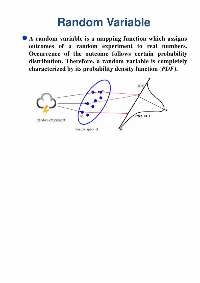
A random variable is a mapping function which assigns

outcomes of a random experiment to real numbers.

Occurrence of the outcome follows certain probability

distribution. Therefore, a random variable is completely

characterized by its probability density function ( PDF).



Random Process

A random variable that is a function of

time is called a random or stochastic

process. Thus a random process is a

collection of infinite number of random

variables.

Examples of random processesDaily stream flow

Hourly rainfall of storm events

Stock index



Stochastic processExample: Let X(t) be the number of people in a particular railway

station from 8Am to t (>=8). Clearly, for each given t, X(t) is a randomvariable. Table below lists some possible values that X(t) could take:

date X(9) X(10) X(11) X(12) X(13) X(14) …

Oct. 12 1360 1412 1750 1603 1598 1821…

Oct. 13 1362 1490 1713 1641 1601 1845…

Oct. 14 1289 1472 1739 1593 1614 1864…

Oct. 15 1313 1453 1721 1631 1622 1871…

Oct. 16 1368 1481 ? ? ? ? ?

Oct. 17 ? ? ? ? ? ? ?



Stochastic Process

• Stochastic processes are processes that proceed randomly in time.

• Rather than consider fixed random variables X, Y , etc. or even

sequences of random variables, we consider sequences X 0, X 1,

X 2, …. Where X

t represent some random quantity at time t .

• In general, the value X t might depend on the quantity X t-1 at time t -1,

or even the value X s for other times s < t .

• Example: people at railway station from 8 AM onwards .



Continuous and Discrete Time Stochastic

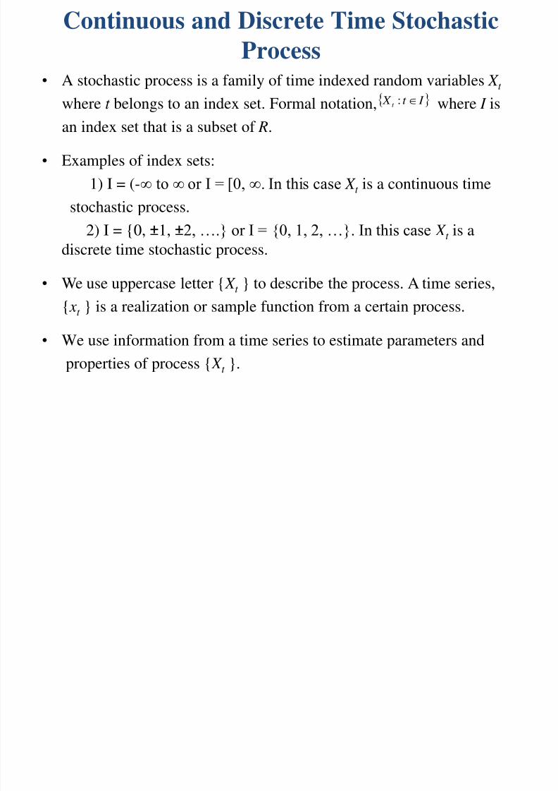
Process• A stochastic process is a family of time indexed random variables X t

where t belongs to an index set. Formal notation, where I is

an index set that is a subset of R.

• Examples of index sets:

1) I = (-∞ to ∞ or I = [0, ∞. In this case X t is a continuous timestochastic process.

2) I = {0, ±1, ±2, ….} or I = {0, 1, 2, …}. In this case X t is a

discrete time stochastic process.

• We use uppercase letter { X t } to describe the process. A time series,

{ xt } is a realization or sample function from a certain process.

• We use information from a time series to estimate parameters and

properties of process { X t }.

I t X t :



Probability Distribution of a Process

• For any stochastic process with index set I , its probabilitydistribution function is uniquely determined by its finite

dimensional distributions.

• The k dimensional distribution function of a process is defined by

for any and any real numbers x1, …, xk .

• The distribution function tells us everything we need to know about

the process { X t }.

k t t k X X

x X x X P x xF k k t t

,...,,...,11,..., 11

I t t k ,...,1



Statistical Averages Summary

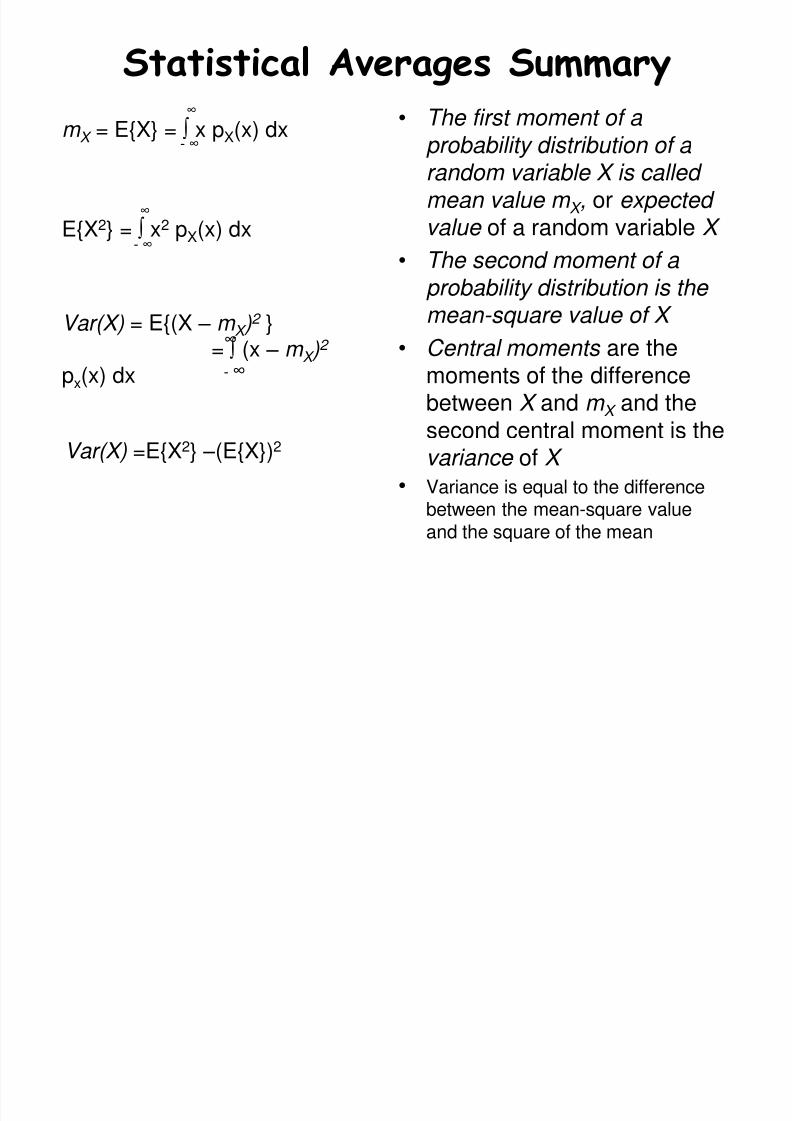
• The first moment of a probability distribution of a random variable X is called mean value m X , or expected value of a random variable X

• The second moment of a probability distribution is the mean-square value of X

• Central moments are themoments of the difference

between X and m X and thesecond central moment is thevariance of X

• Variance is equal to the differencebetween the mean-square value

and the square of the mean

m X = E{X} = ∫ x pX(x) dx- ∞

∞

E{X2} = ∫ x2 pX(x) dx- ∞

∞

Var(X) = E{(X – m X )2 }

= ∫ (x – m X )2

px(x) dx - ∞

∞

Var(X) =E{X2} –(E{X})2



Stationary Processes

• A process is said to be strictly stationary if has the same

joint distribution as . That is, if

• If { X t

} is a strictly stationary process and then, the mean

function is a constant and the variance function is also a constant.

• Moreover, for a strictly stationary process with first two moments

finite, the covariance function, and the correlation function depend

only on the time difference s.

k t t X X ,...,1

k t t X X ,...,1

k X X k X X x xF x xF k t t k t t

,...,,..., 1,...,1,...,11

2

t X E



Weak Stationarity

• Strict stationary is too strong of a condition in practice. It is often

difficult assumption to assess based on an observed time series x1,…, xk .

• In time series analysis we often use a weaker sense of stationary in

terms of the moments of the process.

• A process is said to be nth-order weakly stationary if all its joint

moments up to order n exists and are time invariant, i.e., independent

of time origin.

• For example, a second-order weakly stationary process will have

constant mean and variance, with the covariance and the correlation

being functions of the time difference along.

• A strictly stationary process with the first two moments finite is also a

second-ordered weakly stationary. Also called Wide sense Stationary

process.



Second order stationary process

The Second order density function of asecond order stationary process satisfies

If x(t) is a second order stationary

process then

,,

),,,(),,,(

21

21212121

t t all for

t t x x pt t x x p x x

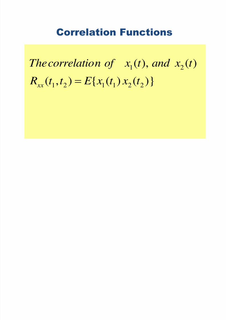
)()}()({},(1111

xx xx Rt xt x E t t R



Wide Sense Stationary

A process is Wide Sense Stationary process if

Second order stationary Wide Sense Stationaryprocess.

•

)()}()({

constant})({

11

xx Rt xt x E

xt x E



Estimation of the mean

• Given a single realization { xt } of a stationary process { X t }, a naturalestimator of the mean is the sample mean

which is the time average of n observations.

t X E

n

t

t xn

x1

1



Sample Autocovariance Function

• Given a single realization { xt } of a stationary process { X t }, thesample autocovariance function given by

is an estimate of the autocavariance function.

k n

t

k t t x x x xn

k 1

1̂



Time Average

The time average of x(t)

T

T T

T

T T

dt t xt xT

dt t x

T

xof AT

)()(2

1lim)(R

isfunctionationautocorreltimeThe

)(

2

1lim..

xx



Ergodic Process

If the time average and time autocorrelation areequal to the statistical average and statisticalautocorrelation then the process is ergodic.

Ergodity is very restrictive. The assumption ofergodity is used to simplify the problem

T

T T

T

T T

dt t xt xT

dx x pt xt x

dt t xT

dx x pt x

)()(2

1lim)())()((

)(21lim)()(



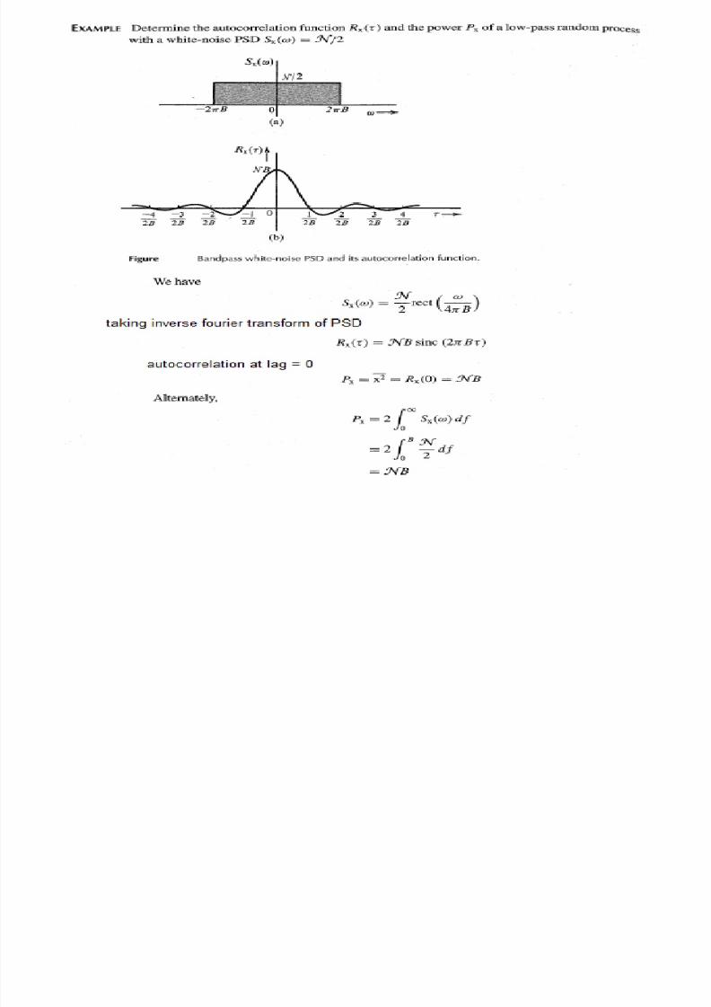
Properties of PSD



Properties of PSD

Some properties of PSD are:

• P x( f ) is always real• P x( f ) > 0

• When x(t ) is real, P x(- f )= P x( f )

• If x(t ) is WSS,

• PSD at zero frequency is:

____

2

Total Normalized Power

0

x

x x

P f df P

P f df P x R

0 x x

P R d



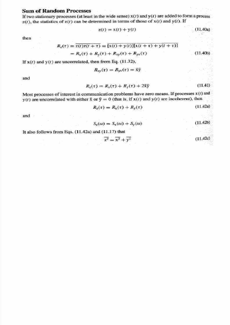
Multiple Random Processes



Linear Systems

• Recall that for LTI systems:

• This is still valid if x and y are random processes, x

might be signal plus noise or just noise

• What is the autocorrelation and PSD for y(t) when x(t)is known?

y t h t x t Y f H f X f

Linear Network

h(t )

H ( f )

x(t )

X ( f )

R x( )

P x( f )

2

( ) ( )

( ) ( ) ( )

y x

y x

y t h t x t

Y f H f X f

R h h R

P f H f P f

Output of an LTI System



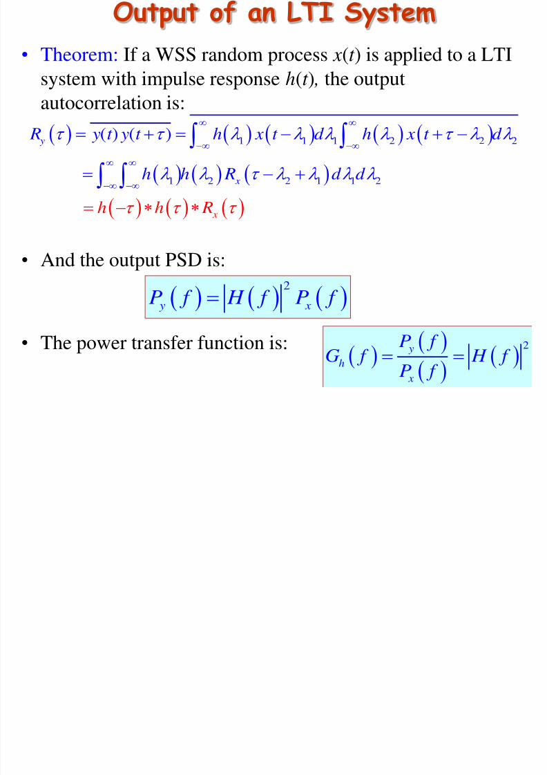
Output of an LTI System

• Theorem: If a WSS random process x(t ) is applied to a LTI

system with impulse response h(t ) , the output

autocorrelation is:

• And the output PSD is:

• The power transfer function is:

1 1 1 2 2 2

1 2 2 1 1 2

( ) ( )

x

y

x

R y t y t h x t d h x t d

h h R d d

h h R

2

y xP f H f P f

2 y

h x

P f G f H f

P f

analog communication lecture 14

Documents