analisis triwulanan: perkembangan moneter, perbankan … vol... · domestic demand. besides,...
TRANSCRIPT


1ANALISIS TRIWULANAN: Perkembangan Moneter, Perbankan dan Sistem Pembayaran, Triwulan II - 2007
BULLETIN OF MONETARY ECONOMICS AND BANKINGCenter for Central Banking Research and Education
Bank Indonesia
PatronDewan Gubernur Bank Indonesia
Editorial Board
Prof. Dr. Anwar NasutionProf. Dr. Miranda S. Goeltom
Prof. Dr. InsukindroProf. Dr. Iwan Jaya Azis
Prof. Iftekhar HasanProf. Dr. Masaaki Komatsu
Dr. M. SyamsuddinDr. Perry Warjiyo
Dr. Iskandar Simorangkir Dr. Solikin M. JuhroDr. Haris Munandar
Dr. Andi M. Alfian ParewangiDr. M. Edhie Purnawan
Dr. Burhanuddin Abdullah
Editorial ChairmanDr. Perry Warjiyo
Dr. Iskandar Simorangkir
Executive DirectorDr. Andi M. Alfian Parewangi
SecretariatArifin M. Suriahaminata, MBA
Nurhemi, MA
The Bulletin of Monetary Economics and Banking (BEMP) is a quarterly accredited journal published by Center for Central Banking Research and Education,Bank Indonesia. The views expressed in this publication are those of the author(s) and do not necessarily reflect those of Bank Indonesia.
We invite academician and practitioners to write on this journal. Please submit your paper and send it via mail: [email protected]. See the writing guidance on the back of this book.
This journal is published on; January – April – August – October. The digital version including all back issues are available online;please visit our link:http://www.bi.go.id/web/id/publikasi/jurnal+Ekonomi/.If you are interested to subscribe for printed version, please contact our distribution department: Statistic Disemination and Management Intern Division - Department of Statistic, Bank Indonesia, Sjafruddin Prawiranegara Building, 2nd Floor – Jl. M.H. Thamrin No. 2 Central Jakarta, Indonesia, phone (021) 2981-6571/2981-5856, fax. (021) 3501912, email: [email protected].

QUARTERLY ANALYSIS : The Progress of Monetary, Banking, and Payment System
Quarter III - 2013
Author Team of Quarterly Report, Bank Indonesia
Systemic Risk And Financial Linkages Measurement In The Indonesian Banking
Sri Ayomi, Bambang Hermanto
Profitability, Growth Opportunity, Capital Structure And The Firm Value
Sri Hermuningsih
Decentralization and Regional Inflation in Indonesia
Darius Tirtosuharto, Handri Adiwilaga
Efficiency of Islamic Banks Using Two Stage Approach of Data Envelopment Analysis
Muhammad Faza Firdaus, Muhamad Nadratuzzaman Hosen
BULLETIN of moNETary EcoNomIcsaNd BaNkINg
Volume 16, Number 2, October 2013
91
137
89
115
155


89QUARTERLY ANALYSIS : The Progress of Monetary, Banking, and Payment System Quarter III 2013
QUARTERLY ANALYSIS:ThE PRogRESS of MoNETARY, BANkINg,
ANd PAYMENT SYSTEM QUARTER III 2013
Author Team of Quarterly Report, Bank Indonesia
Indonesia’s economic growth performed slowly in the third quarter 2013 as previously predicted. Indonesia’s economic growth reached 5.6% (yoy) in the third quarter 2013 where it was relatively slower than the second quarter 2012 reaching 5.8% (yoy). The slowing down economic growth was driven by declining building investment and lower non-building investment growth. Export performance showed relatively better growth even was followed by the increasing total import. Meanwhile, both private and government consumption were positively growing.
Indonesia’s Balance of Payment (BOP) performed deficit pressure in the third quarter 2013. Balance of Payment (BOP) deficit declined to USD8.5 billion compared to the second quarter 2013. This recovery was mainly recorded on balance of trade surplus of non-oil and gas commodities (fob) due to declining non-oil and gas import, in line with the lowering domestic demand. Besides, deficit on balance of service and balance of income declined as well. Nevertheless, deficit on oil and gas balance of trade increased due to declining domestic production and higher oil and gas import for domestic consumption. On the other hand, surplus on balance of Capital and Financial Transaction (CFT) decreased as the impact of declining capital inflow of foreign portofolio due to higher uncertainty of global financial market. Meanwhile, foreign direct investment (FDI) increased driving higher reserve of foreign exchange up to USD95.7 billion by the end of September 2013. The position is equivalent to 5.2 months of imports and government’s foreign debt payments.
In the third quarter 2013, the exchange rate depreciated and was strongly related to fundamental aspects. The depreciation was driven by the increasing uncertainty of global financial market. Depreciate exchange rate had relatively diminished in the end of the quarter in line with the positive response from market agents on postponement of the Fed tapering-off. Performance of the Current Account (CA) was predicted to remain deficit and also influenced the fluctuation of the exchange rate which was at depreciating trend in the third quarter 2013. In average, Rupiah depreciated by 8.18% (qtq) to Rp10,652 per USD from Rp9,781 per USD in the second quarter 2013. Meanwhile, Rupiah depreciated by 14.29% (qtq), point to point, and was closed on Rp11,580 per USD level by the end of the quarter. The relatively high depreciation pressure on Rupiah started from July 2013. Depreciation kept continuing till started to be stable at the end of September on the new equilibrium level which was in line with the economic fundamentals of Indonesia.

90 Bulletin of Monetary, Economics and Banking, October 2013
Slowing down economic growth was driven by high inflationary pressure. CPI inflation significantly increased in the third quarter 2013 compared to the second quarter 2013. CPI inflation grew by 8.40% (yoy) or 4.08% (qtq) at the end of the third quarter 2013 which was higher than the second quarter 2013 growing by 5.90% (yoy) or 0.90% (qtq). It was the impact of the government policy of increasing fuel price at the end of June 2013. The increase of fuel price was driving high administered prices inflation from 6.70-% (yoy) or 4.38% (qtq) in the second quarter 2013 to 15.47% (yoy) or 8.94% (qtq) in the third quarter 2013. The increase of subsidized fuel price also triggered the increase of volatile food inflation by 4.36% (qtq) or 13.94% (yoy) in the third quarter 2013, beside due to the existing supply problem of food during the increasing domestic demand in Ramadhan and Idul Fitri. Nevertheless, the fluctuations of monthly volatile food inflation was in the declining trend. Meanwhile, core inflation increased by 2.59% (qtq) or 4.72% (yoy) in the third quarter 2013 compared to the previous quarter by 0.52% (qtq) or 3.98% (yoy). The increase was mainly influenced by subsequent impact of the increasing fuel price and Rupiah depreciation pressure, while the influence of global commodity price was relatively lower.
The stability of financial system was supported by the solid banking industry. Capital adequacy ratio (CAR) was relatively high up to 18.0% in September 2013, higher than the minimum requirement by 8%, while the ratio of non performing loan (NPL) was relatively lower by 1.86%. Meanwhile, the growth of loan was 23.1% (yoy) in September 2013, higher than the growth on August 2013 by 22.2% (yoy). Nevertheless, the increase of loan was mainly influenced by the impact of Rupiah depreciation revaluation. If the exchange rate remained fixed in the calculation then the growth of loan would be in declining trend by 20.2% (yoy) on August 2013 to 19.9% (yoy) on September 2013. Bank Indonesia assumed that slowing down growth trend of loan was in line with the impact of slowing down domestic economy and was predicted to grow by 18-20% for the whole 2013.
In the third quarter 2013, Balance of Payment (BOP) system declined in terms of value and volume of transactions compared to the second quarter 2013. Transaction value increased by Rp5,069.24 trillion (22.03%) to Rp28,075.62 trillion, while transaction volume increased by 29.52 million transactions (3.01%) to 1,011.75 million transactions. The increase of transaction volume in the third quarter 2013 was driven by the transactions of monetary management that increased by 59.38% from the second quarter 2013 and was in line with the increase of transaction value of monetary operation especially on Deposit Facility instrument. Meanwhile, the increase of transaction volume was mainly driven by the increase of the use of Card-Usage Payment Tool (APMK) which was mainly ATM and/or debit card by 3.04% as the impact of the increasing transaction during Ramadhan and Idul Fitri 2013.

91Systemic Risk And Financial Linkages Measurement In The Indonesian Banking
SYSTEMIC RISK AND FINANCIAL LINKAGES MEASUREMENT IN THE INDONESIAN BANKING
Sri AyomiBambang Hermanto1
This paper measures the insolvency risk of bank in Indonesia. We apply Merton model to identify
the probability of default over 30 banks during the period of 2002-2013. This paper also identify role of
financial linkage a cross banks on transmitting from one bank to another; which enable us to assess if the
risk is systemic or not. The results showed the larger total asset of the bank, the larger they contribute
to systemic risk.
Abstract
Keywords : Conditional Value at Risk; Probability of Default; systemic risk and financial linkages;
Value at Risk.
JEL Classification: D81, G21, G33
1 Sri Ayomi is bank supervisor on Financial Services Authority (OJK); (corresponding author: [email protected]); Bambang Hermanto (may he rest in peace) is lecturer on Economic Department, University of Indonesia, ([email protected]).

92 Bulletin of Monetary, Economics and Banking, October 2013
I. INTRODUCTION
Banking system has a strategic position as the intermediating and supporting payment system institution (UU No. 10/1998). As an intermediating institution, banking can give facilitations to channel the fund from those with excess fund (savers) in the position as the depositors to those who need the fund (borrowers) for various kinds of purposes. Moreover, banking also acts as an agent of development, can encourage the progression of economic improvement through credits facilities and other payment and with drawal facilities in a transaction process done by the economists.
The banking sector is exposed to some risks in doing its function. In order to be able to run its function well, it is required that the banking sector should effectively be able to manage the risks it faces so it can maintain its unremitting business process so the financial intermediating process in economy can run incessantly and efficiently. If the bank is able to reach the optimum efficiency level, it will support the management of the economy so it can function well.
Systemic risk is a determining factor in constructing a country’s economic system stability due to some financial imperfections such as asymetric information, agency problem, and moral hazard which cause excessive risk taking behavior, contagion risk (domino effect) and procyclisation (prosiklisitas) of the financial intermediation.
The systemic risk can also be stated as a risk which can cause the failure of one or some financial institutions as the result of systemic events. This can be in the form of shock which can influence one of the institutions or shock which can influence the institution which then spread to another or a shock which simultaneously affect the majority of other institutions (De Bandt and Hartmann, 2000 and Zebua, 2010). Some researches on systemic risk potential in banking industry, according to Saheruddin (2009), have been done in some European countries (Nagy and Fox, 2005); The United States of America (Buehler and Gupta, 1987); Brazil (Barnhill and Souto, 2007) and in some Asian countries such as Japan (Uchida and Nakagawa, 2004) and Sri Langka (Tennekoon, 2002).
Whereas Adrian dan Brunnermeier (2009) stated that to conduct a measurement which includes systemic risk, it is better to identify the risks which exist in a system by measuring the individual systemic of an institution, in which this institutions are connected to one another and are big in size (too big to fail) so it can cause the negative spillover impact towards other institutions.
Systemic risk becomes a polemic in Indonesia when the government decided to save Century Bank by taking over (bail out) with “much too expensive” costs because the bank was considered as a failed bank and would create a systemic impact. This polemic happens because there is no scientific study or research which covers the banking systemic risks in Indonesia.
The estimation of the bank default probabilities which is carried out by estimating the systemic risk requires two variables; market values and assets’ volatility. In a research conducted

93Systemic Risk And Financial Linkages Measurement In The Indonesian Banking
by Lehar (2005) and Adrian and Brunnermeier (2009), they use the stock price so they can estimate the value. Pennacchi and Redburn (2003) give a model to estimate the assets’ market value and volatility by using the bank’s financial report. The estimation is done not by using balance numbers but based on the profit and loss data. Tudella and Young (2003) verify Merton model to estimate the probability of default of the corporate companies in England so it can determine whether the company is failed or not. However, previously, Black and Cox (1976) did a generalization on the basic model of Merton which studied the obligation effect by including the collateral factors as the variable.
In 2013 Bank of Indonesia as the highest national banking regulator has included systemic surveillance system in the framework of SSK of which main activities include the bank evaluation and LKBB which has systemic risk potentials as well as did some researches and analyses concerning the household, corporate and by sector financial system.
Based on those experiences, the research on systemic risk for banking industry in Indonesia becomes very important to be done considering the effect and huge amount of cost which have to be guaranteed if the crisis shall happen again in the future. With this basic assumption, this paper estimates the systemic risks and the relation of banking finance in Indonesia by identifying the risks of each bank toward the banking system. Since not all of the banks are going public, the measurement of default bank probabilities and the measurement of systemic risk based on its market value and assets’ volatility are estimated by using the bank’s financial report. The estimation is not done by using the balance numbers but based on the profit and loss data.
Explicitly, the aim of this research are, first, to know the probability of default value of each bank based on Merton model; second, to estimate the level of the risks of each bank individually, third, to estimate the contribution of risks from each individual bank toward banking system risk as a whole, fourth, to estimate the change of risks from each individual bank toward banking system risk as a whole; and fifth, to estimate the financial linkage between one bank and the others in Indonesian banking system.
It is hoped that this paper can give positive contributions in the form of new suggestions to banking regulators and other related institutions in arranging banking industry regulations for the materialization of national financial stability and also to enrich the varieties of empirical studies on the systemic risk of banking industry in Indonesia.
The second part of this paper will cover the theory, the third part will cover the data and the applied method, while the estimation result and its analysis will be presented in chapter four. The conclusion and further suggestions will be presented in the fifth chapter as the closing.

94 Bulletin of Monetary, Economics and Banking, October 2013
II. THEORY
The Concept of Systemic Risk and the Bankruptcy of a Bank
The failure risk is the inability of a certain bank to pay for its debt and obligations. Before it is default, there is no other ways to clearly distinguish between the soon to be default bank and not. We only make probabilistic judgements from the failure possibilities. Thus, the bank generally pays the spread on the free-standards level of interests which is comparable with the default probabilities to compensate some loans.
Default is a rare enough phenomenon. Some specifics companies have probability of default for about 2 percent in each year, but there is no variation in the standard probability of the company (Moodys KMV, 2003).
The default in one unit of a company potentially gives influence toward the industry as a whole. According to Adrian and Brunerrmeir (2009) the systemic risk is stated as a possibility if an institution is in distress, this will trigger other institutions in the banking industry to be distressed so it can cause the bank run and the fall of the financial banking system. Whereas according to Acharya (2001), systemic risk is also a shared risk of failure which emerges from the relationship between the return of assets from the balance side of the bank.
De Bandt and Hartmann (2000) propose three interrelated basic characteristics within financial system which can give the basic principals to explain about financial fragility hypothesis, they are:
a. The banking structure or other financial institutions in which the banks generally reserve a few of their assets to fulfill the deposits withdrawal.
b. The interconnectivities of financial institutions through direct exposure and payment system.
c. The intensity of the information from the financial contract and credibility problems which mean the expected asset value in the future and the cash flow guaranteed in the contract will be fulfilled.
The Causes and Indicators of Bankruptcy
Mongid (2000) wrote that according to Hermsillo (1996) the bank failure which is often called as the bankruptcy of a bank consist of two different concepts, the first one is the economic failure or market insolvency; a situation in which the net equity of the bank becomes negative, or if the bank cannot continue its operation without creating loss which immediately result negative net equity. The second is the official failure; it is a type of failure which can be observed because an official agency announces its failure to the public. Official failure happens when the bank regulator states that the institution will not be able to operate in the long term.
95Systemic Risk And Financial Linkages Measurement In The Indonesian Banking
Generally, we can differentiate the sources of bank failure, they are:
1. Overflowing credits expansion of the bank.
2. Asymmetrical information results in the inability of the depositors to value the assets of the bank accurately, especially when the financial condition of the bank is worsen.
3. The shock is started from outside of the banking system, detached from the bank financial condition, which causes the depositors to change their liquidity preferences or it causes the reduction on the bank’s reserves.
4. The institutional limitation and the law which weakens the bank and causes the bankruptcy.
KMV Merton Model
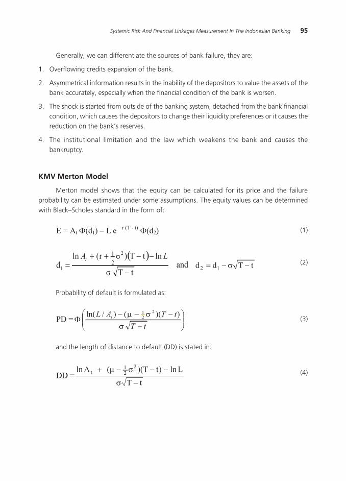
Merton model shows that the equity can be calculated for its price and the failure probability can be estimated under some assumptions. The equity values can be determined with Black–Scholes standard in the form of:
(1)
(2)
(3)
(4)
E = At Ф(d1) – L e – r (T - t) Ф(d2)
( )tTσ
lnand
tT)σ(rlnd
2
121
−
−−++=
LAttTdd 12 −σ−=
Probability of default is formulated as:
PD =
−−−−
ΦtT
tTAL t
σσµ ))(()/ln( 2
21
and the length of distance to default (DD) is stated in:
DD =tT
Lln)tT)((Aln 221
t
−σ
−−σ−µ+

96 Bulletin of Monetary, Economics and Banking, October 2013
and probability of default is summed up into PD = F(-DD).
Cash Flow and Asset Market Value Estimation
Cooperstein, Pennachi and Redburn (1995) estimated the asset market value and its volatility using the financial report and the profit and loss data. The estimation of the auto regressive process equation of the cash flow is done using panel data analysis method.
Figure 1. The probability of default or towards asset value. Default occurs when the final asset value is under the default point (shaded-in area)
Crosbie dan Bohn (2003)
���
�����
����
�����������������������������
����������������������������
��������������� ������������
�����������
����� ���������������������������������������������������
���������������������������������������
���������������������
������������������
������������
�����������������������������������������
��� ������������ ����
Market Equity Et can be calculated as the present value of the whole cash flow expected from the future which:
(5)
(6)
(7)
Ci,t= θt+ρCi,t-1
( )∑∞
=∆+
=∆+
1jj
C
t r1expE
jt
....)r1(
C)1()r1(
C)1()r1(C
3t
32
2t
2t +
+ρ+ρ+ρ+θ
++
ρ+ρ+θ+
+ρ+θ
=∆∆∆
The simpler form:
))(1(C
)(E tt ρ−π−π
πθ+
ρ−πρ
=

97Systemic Risk And Financial Linkages Measurement In The Indonesian Banking
Moreover, according to Loffler and Posch (2007) the estimation of the asset market value and its volatility can be done by iteration approach. The estimation of the stochastic process of the asset of each bank is using Black-Scholes model toward market equity value and the value of account payable ledger. This technique is done by taking the initial volatility value (for example so) to calculate the assets. And then, this asset value is then used to calculate the volatility to calculate the return asset which then is re used again to revise the initial volatility value so (iteration process). The iteration process to k+1 is continued with the calculation of the assets market value which is shown by this equation until the convergence between the volatility of so and s can be achieved.
(8)
(9)
)()(
1
2)(
ddeLEA
tTrt
t ΦΦ+
=−−
Systemic Risk Measurement
The first alternative which can be used is Value at Risk (VaR). VaR is a risk measurement method which uses statistical technique. According to Jorion (2001), VaR is generally defined as a method used to calculate the maximum loss which might happen when it is in a certain period or level of trust.
VaR = μ-α σ
Figure 2. The Distribution of VaR.
����
����
�
��������������
�������
�������
�������������������������������
����������������������
The second alternative is by using financial linkage. The bank risk which correlates one bank to another can be seen from the financial relevance. The concept is how the Value at Risk of the individual bank can be influenced if other banks are in the distress condition. That is why other parameter is needed that is by calculating CoVaR (A|B) which means CoVaR of bank A is conditioned toward bank B which is in distress condition.

98 Bulletin of Monetary, Economics and Banking, October 2013
According to Roengpitya and Rungcharoenkitkul (2010) this concept is considered as an externality which cannot be gained by observing individual risk value only. It is due to the individual risk contribution which is conditioned by the other bank individual risks DCoVaR (A|B) portrayed an amount of excess from the Value at Risk of bank A which is separated from Value at Risk of bank A itself which caused by bank B. Whereas to calculate the additional percentage of the value at risk towards bank A when the value at risk of bank B is in distress condition, it is using % DCoVaR (A|B). The bigger percentage of the value at risk contribution of bank B toward the value at risk of bank A, the more systemic bank B is toward bank A.
3. METHODOLOGY
Data Collection Technique
This research is exploratory in nature in evaluating the systemic risk of individual bank towards the banking system. There are four data processing techniques used as explained below.
The first step is calculating the banking assets; market value, especially for the banks who have not gone public yet. Cooperstein, Pennacchi and Redburn (2003) give a model to estimate the market value and volatility of the assets by using the bank’s financial report. In this paper, the estimation of market value of the bank assets is done by using the profit and loss report data.
The return assets of each bank and the return assets of the banking system is stated as:
(10)
(11)
−=
−
−i
1t
i1t
iti
t AAA
X and
−=
−
−sys
1t
sys1t
systsys
t AAA
X
with ∑=i
it
syst AA . sys
tX shows the return of the total assets of the whole banking system; and sys
1tA − shows the total assets of the banking system in the previous period.
To gain the time variation of the distribution between Xi and Xsys, this distribution is estimated as the function of a string of macro variables which can influence the amount of assets return. In this stage, the data processing technique used is Generalize Autoregressive Conditional Heteroschedasticor GARCH (1,1). The equation specification to estimate the return value of the bank assets is:
it
iiit MX ε+β+α=
syst
syssyssyst MX ε+β+α=

99Systemic Risk And Financial Linkages Measurement In The Indonesian Banking
The second stage is calculating the probability of default of the individual bank and banking system in general. Lehar (2005), and Adrian and Brunnermeier (2009) uses the stock price to estimate this probability of default quantity. In this research, we estimate the value VaR individual dan VaR banking system using this specification:
with VaRti as the value at risk of bank i in the period of t, and VaRt
sys as the value at risk of the banking system within the period of t. M is the macro variable vector which includes SBI, JIBOR and IHSG; all of those three are calculated in their growth value.
(12)
(13)
(14)
(15)
MˆˆVaR iiit β+α=
MˆˆVaR syssyssyst β+α=
SBIt =1t
1tt
SBISBISBI
−
−− JIBORt =
1t
1tt
JIBORJIBORJIBOR
−
−− IHSGt =
1t
1tt
IHSGIHSGIHSG
−
−−
The third step is calculating the parameter of Conditional Value at Risk (CoVaR) which is based on the Value at Risk of the individual bank and the whole banking system. This quantity of CoVaR actually reflects the systemic risk in the term of the influence of a bank towards the banking system as a whole. Technically, the estimation of CoVaRt
i is done by using the coefficient of the banking system estimation result and substitute the result of the VaRt
i estimation result towards the coefficient of gsys|i:
isyst
it
isysisysisyssyst XMX |||| εγβα +++=
it
isysisysisysit VaRMCoVaR ||| ˆˆˆ γβα ++=
where: CoVaRti as the conditional value at risk of the banking system in the VaR of bank
i; whereas as the estimated parameter. The next step is to do calculation on systemic risk contribution from the banking system of each individual bank in the form of:
syst
it
it VaRCoVaRCoVaR −=∆
The fourth step in the data processing stage is the calculation of financial linkage. In this paper, these four stages are used:
a. Analyzing the equation of CoVaR(A|B) which becomes the value at risk of bank A which is conditioned towards the value at risk of bank B:

100 Bulletin of Monetary, Economics and Banking, October 2013
b. The CoVaR (A|B) estimation
(16)
(17)
(18)
(19)
B,At
Bt
AAt XMX ε+γ+β+α=
CoVaR(A|B)t = Bt
AA VaRˆMˆˆ γ+β+α
c. The level of marginalization or the change of DCoVaR(A|B):
ΔCoVaR(A|B)t = CoVaR(A|B)t – VaR(A)t
d. The inter-bank financial linkage analysis by measuring the percentage of the risk changes of bank A conditioned by bank B:
% ΔCoVaR(A|B)t = t
tt
VaR(A)VaR(A) - B)|CoVaR(A
Data Source
The data in this research includes the monthly cash flow, the capitalization equity, assets and debt values as well as macro variables data (SBI rate, JIBOR dan IHSG) also includes the monthly financial report within the period of 2002 – 2013. The data source of the research is gained from the publication result of 30 public banks which have been go public and have not yet been go public. It includes 10 banks with the total assets of more than Rp50 quintillion, 10 banks with the total assets of more than Rp10 quintillion until Rp50 quintillion and 10 banks with the assets of lower than Rp10 quintillion.
The financial report is achieved from the CFS bank reports to the Bank of Indonesia and the interest rate of SBI is achieved from Bank of Indonesia. JIBOR is achieved from Indonesian Capital Market Directory and IHSG is originated from Indonesian Stock Market (Bursa Efek Indonesia/BEI) sites.
IV. RESULT AND ANALYSIS
4.1 Probability of Default Analysis
The default condition of a bank will potentially influence other banks so there will be some systemic risks problems. Thus, the failure of a certain bank is a risk which has to be measured and responded rationally, so the attempt on the prevention of the failure of the bank must be done since the early stages.

101Systemic Risk And Financial Linkages Measurement In The Indonesian Banking
There are many factors which influence the payment failure of a bank. The return of the assets market value and its volatility are the required main factors to calculate the probability of default in Merton model. Before it is in default condition, there is no other way that can clearly differentiate between the banks which will be in the default condition and not. We can only observe and calculate its default chance. In this term, each bank will pay insurant which is comparable with the probability of default to compensate the loaner for this indeterminacy.
The result of this research shows that for big banks, the accumulation of the average default risk probability reaches 42,36 percent during the research period. The maximum average probability of default is 93,62 percent, it was found in Bank T which has the lowest rating of
��������������������������������������������������
������ ��������� ������ ������������ ��������� ��������� ������ ������������ �������� ��������� ������ ������������ �������� ��������� ������ ������������ ������� �������� ������ ������������ ������� �������� ������ ������������ �������� �������� ������ ������������ �������� �������� ������ ������������ ��������� �������� ������ ������������ ������� �������� ������ ������������ �������� ������� ������ ������������ �������� �������� ������ ������������ ������� ������� ������ ������������ ������� �������� ������ ������������ �������� ������� ������ ������������ ��������� ������� ������ ������������ �������� �������� ������ ������������ �������� �������� ������ ������������ �������� ������� ������ ������������ ������� ������� ������ ������������ ������� ������� ������ ������������ ������� ������� ������ ������������ �������� ������� ������ ������������ �������� ������� ������ ������������ ������� ������� ������ ������������ ������� ����� ������ ������������ �������� ����� ������ ������������ ���������� ����� ������ ������������ ���������� ����� ������ ������������ ��������� ����� ������ ������������ �
��������������������������������������� ���������������������������������������������
������������������������������������������������������������������������������������������������������������
���������������
������������������������� ����������
������������������������������
������������������������
������

102 Bulletin of Monetary, Economics and Banking, October 2013
C. Whereas its minimum average reaches 16,9 percent which is the default risk of Bank D, which has the rating of A.
Referring to the migration matrix, it can be observed that the potential of Bank D to have the default risk in the span of one year is very small with the amount of 0,04 percent. Moreover to the bank which is in unstable condition, the probability of bankruptcy or area is also small which is only in the amount of 0,01 percent. Generally, the banks with the rating of A has the risk probability which is still under 1 percent that is 0,04 percent. However, the chance of migration to the rating of AAA (companies with the best quality, proper and stable) is also small with 0,07 percent.
There is a big enough chance of migration from the banks with the rating of A to the rating of AA in the amount of 2,25 percent. However, the number is still considered as low because it is still under 5 percent. While the migration probability of the banks with the rating of BBB to the rating of A or from the rating of BB is almost the same with the amount of 4 percent, and the chance to maintain in the same rating within one year is almost 90 percent.
Bank A and Bank H are included in the classification of BBB with the probability of default value of 35 percent. This bank can be called as a healthy bank and the financial condition is satisfactory. The ability to maintain the rating of BBB is big enough that it reaches 89,3 percent. However, the chance to elevate the rating to A, AA or AAA is also low, each with the migration probability of 4,83 percent; 0,25 percent and 0,03 percent. Although it is difficult to elevate, the default and bankruptcy probability is also very small which is 0,22 percent.
4.2. Systemic Risk Analysis
VaR of Individual Bank and VaR of the System
The result of the estimation shows the mean or average of individual bank VaR reaches -29,87 percent. This amount of average VaR is contributed by the VaR from Bank Sand Bank T which is more than 50 percent. These two banks have a low performance with the rating of C. Aggregately, the VaR of the banking system in Indonesia has a small probability of default, which is shown by the VaR of the system with the amount of -3,04 percent.
According to the result of the research, the banks with low performances such as Bank S, Bank T and Bank X, have much bigger return asset fluctuation than the other banks. This paper confirms that the average value of those banks’VaR is the biggest VaR compared to the other banks’ VaR, it shows a very big individual risk in those Bank S, Bank T and Bank X.
103Systemic Risk And Financial Linkages Measurement In The Indonesian Banking
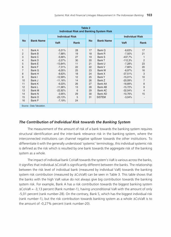
The Contribution of Individual Risk towards the Banking System
The measurement of the amount of risk of a bank towards the banking system requires structural identification and the inter-bank relevance risk in the banking system, where the interconnected institutions can channel negative spillover towards the other institutions. To differentiate it with the generally understood ‘systemic’ terminology, this individual systemic risk is defined as the risk which is resulted by one bank towards the aggregate risk of the banking system as a whole.
The impact of individual bank CoVaR towards the system’s VaR is various across the banks, it signifies that individual DCoVaR is significantly different between the banks. The relationship between the risk level of individual bank (measured by individual VaR) towards the banking system risk contribution (measured by DCoVaR) can be seen in Table 3. This table shows that the banks with the high VaR value do not always give big contribution towards the banking system risk. For example, Bank A has a risk contribution towards the biggest banking system DCoVaR = -3,13 percent (Rank number-1), having unconditional VaR with the amount of only -5,01 percent (rank number-28). On the contrary, Bank S, which has the biggest individual risk (rank number-1), but the risk contribution towards banking system as a whole DCoVaR is to the amount of -0,27% percent (rank number-20).
����������������������������������������������
� ������� ������ �� �� ������� ������ ��� ������� ������ �� �� ������� ������ ��� �������� ������ �� �� ������� ������� �� ������� ������ �� �� ������� ������� �� ������� ������� �� �� ������� ������ ��� ������� ������ �� �� ������� ������ ��� ������� ������ �� �� ������� ������ ��� ������� ������ �� �� ������� ������� �� ������� ������� �� �� ������� ������� ���� ������� ������� �� �� ������� ������� ��� ������� ������ �� �� �������� ������� ��� ������� ������� �� �� �������� ������� ��� ������� ������� � �� �������� ������� ��� ������� ������ �� �� �������� ������� ���� ������� ������� � �� ������ ������ ��� ������� ������ ��
�������������������������
�����
���������������
�������������
�����
���������������
�������������

104 Bulletin of Monetary, Economics and Banking, October 2013
The percentage of the individual bank risk contribution toward the system, is linearly connected with the amount of the bank’s contribution towards the banking system risk aggregately. The higher the risk contribution, the closer its potential systemic impact towards banking aggregately is. According to the writer, the risk contribution towards banking can be categorized as having systemic impact if the risk contribution has reached more than 10 percent.
In this term, the main point regarding the issues of systemic risk is when one bank is in a trouble, so it will create panic in the financial system, so in the end it will cause the failure of other institutions. This can lead to a financial crisis. The most alarming thing is the simultaneous failure of some banks will create a serious financial crisis due to the impact of banking crisis towards the economy is huge. Hoggarth (2002) found that the simultaneous failure causes the reduction of PDB output with the average of 15 - 20 percent during the crisis.
Referring to the threshold of 10 percent above, this research has categorized which banks which have the potential to give systemic impact towards the banking system as a whole. The result of the calculation (Tabel 3) shows that form the 30 banks observed, there are 19 banks which have the potential to give systemic impact towards the banking system, they are Bank A, Bank B, Bank C, Bank D, Bank O, Bank G, Bank F, Bank AA, Bank Y, Bank X, Bank E, Bank K, Bank Z, Bank H, Bank L, Bank I, Bank U, Bank J, Bank W.
Figure 3. Banking System VaR and Bank’s CoVaR
����
����
����
����
����
����
���
�� �� �� �� �� �� �� �� �� �� ��
���������� ������������������������������������
������������
����
����
����
����
����
����
���
���������� ��������������������������������
�������
�� �� �� �� �� �� �� �� �� �� ��

105Systemic Risk And Financial Linkages Measurement In The Indonesian Banking
It is interesting to analyze that the level 19 banks which are categorized as having potential to give systemic impact towards banking, precisely to have good enough rating from B to A and only two of them having the rating of CCC that are bank AA and bank O. On the other hand, the bank which is categorized as not having potential to give systemic impact towards banking system has the rating span from CCC to BB. However, as what has been stated in the beginning that this research is an explorative research and the result of the calculation in this model at least can contribute the measurable discussion foundation for all of the economic stakeholders.
������������������������������������������������������
������� ������ �� ������ � ������� ��������� ���������� ������ �� ������ � ������ �������� ���������� ������ �� ������ � ������ �������� ��������� ������ �� ������ � ������ �������� �������� ������� � ������ � ������ �������� ���������� ������ �� ������ � ������ �������� ��������� ������ �� ������ � ������ �������� ���������� ������� � ������ � ������ �������� ���������� ������� �� ������ � ������ �������� �������� ������� � ������ �� ������ �������� �������� ������� �� ������ �� ������ �������� �������� ������ �� ������ �� ������ �������� ��������� ������ �� ������ �� ������ �������� ���������� ������� � ������ �� ������ �������� �������� ������� �� ������ �� ������ �������� �������� ������� �� ������ �� ������ �������� �������� ������ �� ������ �� ������ �������� �������� ������� �� ������ �� ������ �������� ��������� ������ �� ������ �� ������ �������� ��������� ������� � ������ �� ����� ������������ ��������� ������� � ������ �� ����� ������������ ���������� ������ �� ������ �� ����� ������������ ���������� ������� � ������ �� ����� ������������ ��������� ������ �� ������ �� ����� ������������ ��������� ������� � ������ �� ����� ������������ �������� ������� � ������ �� ����� ������������ ��������� ������� �� ������ �� ����� ������������ �������� ������ �� ����� �� ������� ������������ ��������� ������ �� ����� �� ������� ������������ ��������� ������ �� ����� �� ������� ������������ ��������� � � � � ������ �
��������������������������
����
��������������� ���������������������������������������������
�������������������������
��� ����
������������������������������������������������
������� ���� �������

106 Bulletin of Monetary, Economics and Banking, October 2013
The Banking Financial Linkage
Some previous studies concluded that when smaller banks are in distress condition and declared as bankrupt it does not mean that those banks will not give huge systemic impact. It is due to the possibilities of bank run or bank panic which can emerge because the condition happens, especially, when the macroeconomic condition is having a downturn (economic recession). The study done by Simorangkir, (2006) stated that the pressure of the macroeconomic condition in Indonesia which happened in 1997-1998 significantly impacted towards the occurrence of bank runs during the period of banking crisis at that time.
In general, it can be stated that the bank, individually, has externality towards the occurring system so the assessment towards the systemic risk potential of certain individual banks should be the center of attention of the regulator. According to Roengpitya and Rungcharoenkitkul (2009) the banks which seem to operate in a prudent way and have lower individual risk, are also possible to be able to threaten the viability of the banking system stability especially in a certain condition.
According to the writer’s consideration, financial linkage CoVaR (A|B) can significantly be seen as having inter-bank systemic risk impact if the level of contribution percentage %DCoVaR(A|B) reaches more than 10 percent. If a bank has high level of financial linkage with other banks, when it is bankrupt, the other banks will get bigger impact.
Table 4 shows that banks which have the average of %DCoVaR < 10% or non-systemic towards the banking system also have the average of %DCoVaR (A/B) < 10% or non-systemic towards the other banks. Whereas from 19 banks which have the average of %DCoVaR > 10% or systemic towards the banking system, 13 banks among them have the average of %DCoVaR (A/B) > 10% or systemic towards other banks and 6 of them have the average of %DCoVaR (A/B) < 10% or non-systemic towards the other banks.
However, further investigation can be done by observing Table 5. We can see that bigger banks such as bank A, B, C and D can condition the risk of other individual banks’ VaR with big enough percentage. For example, Bank A has the individual VaR level of -5.01 percent; the contribution of conditional value at risk of Bank A towards Bank E or DCoVaR (E|A) is to the amount of -2.73 percent and the contribution percentage of %DCoVaR (E|A)is to the amount of 19.75 percent. On the other hand, Bank E with the individual VaR level of -13.84 persen; the contribution of conditional value at risk of bank E towards Bank A is only to the amount of -0.27 percent and the percentage of %DCoVaR (A|E) is to the amount of 5.43 percent. It shows that Bank A can increase the risk towards Bank E from the VaRof -13.84 percent into -16.57 percent (systemic risk potential). On the other hand, Bank E can only increase the VaR risk of Bank A from minus -5.01 percent into just -5.29 percent (non systemic risk potential). The interesting thing is when we observe the medium bank S which has not so big amount of asset and non systemic towards the banking system, can only condition 6 other banks with %DCoVaR (A/B) > 10% which is towards 78.48% from the VaR of bank E, 14.60% from the

107Systemic Risk And Financial Linkages Measurement In The Indonesian Banking
VaR of bank J, 35.62% from the VaR of bank P, 29.44% from the VaR of bank Q, 27.87% from the VaR of bank R and 11.35% from the VaR of Bank Y. Bank E can condition to the amount of 14.43% towards the VaR of bank C, in which Bank C can condition the other banks with big enough percentage since it is systemic in nature. Furthermore, Bank J can condition bank E, F, G, H where bank F and G can big enough condition bank A, B, C, D and E. Bank A, B, C and D are systemic in nature. It goes furthermore, the other banks will condition each other towards other banks. Thus, when smaller banks are in distress condition and declared as bankrupt it does not mean that those banks will not give huge systemic impact
Theoretically, if there is a strong negative effect from the bank failure of one or more banks, the bank will be encouraged to invest in the same industry to be able to survive or fail altogether. This strategy is called as collective risk. The consequence of this strategy is that the bank will have asset which has higher correlation which leads to the higher possibility of collective banking failure. Acharya (2001) mentioned the occurrence of “negative externality,” which in fact depends on the size of the failed banks, the uniqueness of the failed banks, and the cases in which the operating banks do not benefited and do the failed bank facilities takeover.
The spreading of the failed bank risk through the interconnection of institutions can originate from the failure of the coordination and liquidity crisis. The credence crisis does not have to originate from the failure risk of the opponent but it might originate from the deteriorating of certain spiral of asset value. However, there are other reasons in some literatures which state that the systemic risk is only the matter of coordination. Thus, the spreading of the crisis towards the liquidity to other institutions will give a systemic spreading impact towards banking. That is why, the systemic risk which caused by the lacking of liquidity in a financial system will give bigger impact to other banks at the times when the shock is spreading rapidly.

108 Bulletin of Monetary, Economics and Banking, October 2013
�����������������������������������������������������������������
������ ����� ����� ������ ������ ����� ����� �������������� ����� ����� ����� ������ ����� ����� ��������������� ����� ����� ����� ������ ����� ����� �������������� ����� ����� ����� ������ ����� ����� �������������� ����� ����� ����� ������ ����� ���� ������������������ ����� ����� ����� ������ ����� ����� �������������� ����� ����� ����� ������ ����� ����� �������������� ����� ����� ����� ������ ���� ���� ������������������ ����� ����� ����� ������ ����� ���� ������������������ ����� ����� ����� ������ ������ ���� ������������������ ����� ����� ����� ������ ����� ���� ������������������ ����� ����� ����� ������ ����� ����� �������������� ����� ����� ���� ������ ����� ���� ������������������ ����� ����� ���� ������ ���� ���� ������������������ ����� ����� ����� ������ ����� ����� �������������� ����� ���� ������ ������ ����� ���� ������������������ ����� ���� ������ ������ ����� ���� ������������������ ����� ���� ������ ������ ����� ���� ������������������ ����� ����� ���� ������ ����� ���� ������������������ ����� ����� ���� ������ ����� ���� ������������������ ����� ����� ����� ������ ����� ����� �������������� ����� ����� ���� ������ ����� ���� ������������������ ����� ����� ����� ������ ����� ���� ������������������ ����� ����� ����� ������ ����� ����� �������������� ����� ����� ����� ������ ����� ����� �������������� ����� ����� ����� ������ ���� ����� ��������������� ����� ����� ����� ������ ����� ����� ��������������� ����� ����� ���� ������ ���� ���� ������������������� ����� ����� ���� ������ ����� ���� ������������������� ����� ����� ���� ������ ����� ���� ������������
�������������������������������������������������������������������������������������������������������
����
���������������������� ����������������������
����������������������
����������������������������������������
���������������������������
����� ������������������������������
������������������
��������������
�����

109Systemic Risk And Financial Linkages Measurement In The Indonesian Banking
�����
�����
���
�����
���
�����������
���
����
���
����
����
�������
�����
���������
��������
���
����
���
����
��
��
��
��
��
��
��
����
�������
���
����
����
����
���
����
����
���
����
����
����
����
����
����
����
����
�����
���
����
����
����
���
����
����
����
����
���
����
����
����
����
����
����
�������
���
����
����
����
����
����
����
���
����
���
����
����
����
���
����
����
�����
���
����
����
����
����
����
����
����
����
���
����
����
����
���
����
����
�����
���
����
����
����
���
����
����
����
���
����
���
����
���
���
����
����
�������
���
����
����
����
���
���
����
����
����
����
���
����
����
���
����
����
�������
���
����
����
����
����
���
����
����
����
����
����
���
����
���
����
����
�����
���
���
����
���
����
����
����
����
����
����
���
����
���
����
���
���
��������
����
����
����
����
����
����
����
����
����
����
���
����
���
���
����
���
������
���
����
���
���
���
����
����
����
����
����
����
����
����
���
���
���
�������
���
����
����
����
����
���
����
����
���
����
����
����
����
���
����
���
�����
���
����
����
����
����
���
����
���
����
���
����
����
����
����
����
���
�����
���
����
����
���
����
���
����
���
���
���
����
���
���
���
���
����
���
����
����
�����
���
���
����
����
����
����
����
����
����
����
����
����
���
���
����
���
�����
���
����
����
����
����
���
����
����
���
����
����
���
����
����
����
���
���
�����
�����
����
����
����
����
���
����
����
���
���
���
���
����
���
����
����
���
�������
����
���
���
���
����
����
����
����
����
����
����
����
����
����
����
���
���
����

110 Bulletin of Monetary, Economics and Banking, October 2013
�����
�����
���
�����
���
�����������
���
����
���
����
����
�������
�����
���������
��������
���
����
����
�����������
�
����
��
��
��
��
��
���
��
��
��
���
�������
���
���
����
���
����
����
����
����
����
����
����
����
����
����
����
����
����
�����
���
���
����
���
����
����
����
����
����
����
����
����
����
����
����
����
����
�����
���
���
����
���
����
����
����
����
����
����
����
����
����
����
����
����
����
�����
���
���
���
���
����
���
���
����
����
����
����
���
����
���
���
���
�������
���
���
���
���
����
����
����
���
����
����
����
���
���
����
����
���
�����
���
���
����
���
���
���
����
����
���
����
����
����
���
���
����
���
����
���
�����
���
����
����
����
���
����
����
���
����
����
����
���
����
����
����
���
�����
���
����
����
����
���
����
����
���
����
���
����
����
����
���
����
����
����
����
�����
���
���
���
���
����
����
���
���
����
����
����
����
����
����
���
���
�������
���
����
����
����
����
���
����
����
���
����
����
����
���
���
���
����
�����
���
���
����
���
���
����
����
���
����
���
����
����
���
����
���
����
���
���
�����
��
����
����
����
���
���
����
���
����
����
����
���
����
���
����
����
�������
��
���
���
���
����
���
���
����
����
����
���
����
����
����
���
����
���
�����
��
����
����
����
���
���
����
���
���
���
����
���
���
���
����
���
���
���
�������
��
����
���
���
����
���
���
����
����
����
���
���
����
���
����
���
���
���
����
���
����
���
���
���
���
���
���
����
���
���
����
����
����
����
���
���
����
���
�������
����
���
���
���
����
���
���
���
���
����
���
����
����
����
����
����
���
���
���

111Systemic Risk And Financial Linkages Measurement In The Indonesian Banking
V. CONCLUSION
This research gives some interesting empirical conclusions which can become an opening discourse on banking systemic risk. By using 30 public banks as the research sample, the empirical conclusion which can be gained are, first, the average probability of default of the bank during the research period (2002 – 2013) is to the amount of 53,60 percent with the deviation standard of 4,81 percent. Merton model has enough special qualities because it does not need assumptions on the functional forms which used both as the early risk signal and the potential of probability of default.
The second empirical finding is that the default banking probability is highly influenced by the amount of volatility return of the bank’s asset. The higher the volatility fluctuation, the bigger the risk potential of a bank to be in default condition is and or vice versa too.
On the individual bank level, the third empirical finding is that the VaR risk of individual bank is found with the average amount of -29,87 percentand VaR of banking system is only to the amount of -3,04 percent. This unconditional VaR value of each bank can be used to portray how big the risk is towards the banking system.
With the analysis of interbank financial linkage, this research gives the fourth conclusion that the individual bank risk which is conditioned towards the other individual bank risks has the average CoVaR(A|B) to the amount of -31,07 percent. Each bank gives different additional risk when the bank is in distress.
The average amount of the additional risk contribution of the bank which is conditioned by the other banks is to the amount of-1,21% and the average of contribution percentage %DCoVaR(A|B) is to the amount of 9,69 percent. This parameter is actually linearly related with the amount of systemic risk contribution. The higher the risk contribution, the higher the systemic risk contribution percentage is. This is the fifth empirical finding.
Those five empirical findings above show that generally, each bank has externality towards banking system as a whole, so the assessment on the potential of systemic risk in certain individual banks deserve to be noted by the regulator. Smaller banks or the banks which seem to operate in a prudent way and lower individual risk, are not possible to threaten the sustainability of the banking system stability especially in some certain conditions.The empirical finding in this research needs to be considered by both the government and the financial authority (Bank of Indonesia,Financial Service Authority or Lembaga Penjamin Simpanan (Saving Assurance Institution)), to be made as a suggestion in the creation of the more accurate rules and policies.
This research needs further improvement first on the term of the amount of data observed and the number of the observation needs to be increased; second, the need to consider the roles of external factors in the modeling of the financial linkage equations; the third, the need to confront and further analyze the amount of the threshold used in determining the banking systemic risk.

112 Bulletin of Monetary, Economics and Banking, October 2013
REFERENCES
Acharya, Viral V. (2009). A Theory of Systemic Risk and Design of Prudential Bank Regulation.
PhD Dissertation of New York University
Adrian, t., dan Brunnermeier, (2009). Covar. Princeton University, Department of Economics, Bendheim Center for Finance, Princeton,
Black, F and Cox, J (1976), ‘Valuing corporate securities: some effects of bond indenture
provisions’, Journal of Finance, Vol. 31, pages 351–67.
Cooperstein, R.,L., Pennacchi, G.G. Redburn, F.S. (2003). The Aggregate Cost of Deposit
Insurance: A Multiperiod Analysis, Deparment of Finance University of Illinois.
Crosbie, P and Bohn, J. (2003). Modelling Default Risk. Moody’s KMV Company.
De Bandt, O. and P. Hartmann, (2000). Systemic Risk: A Survey, CEPR Discussion Paper Series No. 2634.
Foster, G. (1986). Financial Statement Analysis. 2nd Ed. Prentice Hall.
Heffernan, S. (2005). Modern Banking. West Sussex. Joh Willey and Sons Ltd
Jorion, P. (2001). Value at Risk. 2nd ed., McGraw-Hill, New York.
KMV, (2003). Modeling Default Risk, Published by: Moody’s KMV Company.
Lehar, Alfred. (2005). Measuring Systemic Risk: A Risk Management Approach, Journal of
Banking & Finance 29. Department of Business Studies, University of Vienna, Vienna, Austria.
Malik,I., (2013). Premi Berbasiskan Risiko Pada Lembaga Penjamin Simpanan. Program Pascasarjana, Universitas Indonesia. Jakarta.
Merton, R.C. (1974). On the Pricing of Corporate Debt: The Risk Structure of Interest Rates. The Journal of Finance, Volume 29 Issue 2. New York.
Mongid, A. (2000). ”Accounting Data and Bank Future Failure: A Model For Indonesia. Simposium Nasional Akuntansi
Roengpitya, R. dan Rungcharoenkitkul, P. (2010). Measuring Systemic Risk And Financial Linkages
In The Thai Banking System, Bank of Thailand, Jurnal Bank of Thailand, Bangkok.

113Systemic Risk And Financial Linkages Measurement In The Indonesian Banking
Saheruddin, H. (2009). Mengungkap Praktek Herding pada Perbankan Indonesia dengan Metode K-Means Cluster dan LSV Measure: Implikasinya Terhadap Risiko Sistemik. Tesis, Fakultas Ekonomi, Universitas Indonesia, Jakarta.
Tudela and Young, G., (2003). A Merton Model Approach to Assessing the Default Risk of UK
Public Companies Bank of England.
Zebua, A., (2010). Analisis Resiko Sistemik Perbankan di Indonesia. Program Pascasarjana, Institut Pertanian Bogor (IPB), Bogor.

114 Bulletin of Monetary, Economics and Banking, October 2013
Halaman ini sengaja dikosongkan

115Profitability, Growth Opportunity, Capital Structure And The Firm Value
PROFITABILITY, GROWTH OPPORTUNITY, CAPITAL STRUCTURE AND THE FIRM VALUE
Sri Hermuningsih1
This paper examines the influence of profitability, growth opportunity, and capital structure on
firm value. We apply Structural Equation Model (SEM) on 150 listed companies on the Indonesia Stock
Exchange during 2006 to 2010. The result shows that profitability, growth opportunity and capital structure
positively and significantly affect the company’s value. Secondly, the capital structure intervene the effect
of growth profitability on company’s value, but not for profitability.
Abstract
Keywords: profitability, growth opportunitiy, capital structure, firm value, SEM.
JEL Classification: C51, G32, L25
1 Lecturer at Economic Department, University of SarjanawiyataTamansiswaYogyakarta; [email protected].

116 Bulletin of Monetary, Economics and Banking, October 2013
I. INTRODUCTION
The main goal for a firm going public is to increase the shareholder welfare by increasing the value of a firm (Salvatore, 2005). The firm value is very important, as higher firm’s value will increase the welfare of the stockholder (Bringham and Gapensi, 2006). The increase of stock price will also increase the value of the firm. The welfare of the shareholder and value of the firm are commonly represented on the stock price, which implicitly represent the investment decision, financing and asset management.
Weston and Brigham (1998) underline the financial leverage as the way to finance the activa; the right side of balance sheet, while the capital structure represents the permanent financing mainly as long term debt, preferred stock and common stock, and part of short term debt. This emphasizes that the capital structure is only part of financial structure of the firm.
Many factors may influence the value of the firm; among others are profitability, growth opportunity, and capital structure. Profitability shows the ability of the firm to gain profit during certain period. Husnan (2001) define profitability as the ability of the firm to raise profit from sales, asset, and certain capital stock. On the other hand, Shapiro (1991) defines profitability as the ability of the firm to gain profit using all capital they have; “Profitability ratios measure
management’s objectiveness as a indicated by return on sales, assets and owners equity”.
Profitability is important on maintaining the firm activity in the long run, and reflects the prospect of the firm. This way all firms will try to increase their profitability on assuring their business continuance. Profitability also reflects the efficiency of management, measured with the yield of return. Profitability ratio may be indicated by profit margin, basic earning power, return on asset, and return on equity. On this paper, we measure profitability with return on equity (ROE). The ROE shows the ability of the firm to gain net profit for the shareholders; the greater ROE the greater the performance of the firm is. The increase of ROE represents an increase of management efficiency on managing the fund and operational activities to create profit. The growth of ROE indicates higher profit potency and better prospect of the firm. This will be good signal for the investors, increase their trust, and therefore enable the management to increase equity capital of the firm. On the other side, when the demand for firm’s stock increase on the market, it will increase its equilibrium price.
Growth opportunity is the probability of the firm to grow (Mai, 2006). Firms which are expected to grow highly in the future tend to use stock to finance their operational activity. On the opposite, for this reason the firms with low growth opportunity usually use long term debt as their source of financing. Since the growth opportunity varies across firms, their financing decision my management will also vary. Firms with good growth opportunity tend to use their own capital to avoid under investment; a condition where positive value investment projects failed to implement, (Chen, 2004). In addition, the effect of capital ownership and debt policy may influence on firm value is subject to tax, agency cost, and financial difficulty due to the use

117Profitability, Growth Opportunity, Capital Structure And The Firm Value
of debt. Based on trade off model, optimal capital structure is a balance between tax savings and the debt fee, since the cost and the benefit of debt will cancel out. The optimal debt is gained when the interest tax-shield reach the limit of the cost of financial distress. We may expect the firm to reach its optimum value on optimum debt condition. When the value of debt exceeds its optimum or exceed financial distress cost, the debt will negatively affect the firm value.
Based on the capital structure theory, as the capital structure exceeds its optimum, and then each additional debt will reduce the value of the firm. Decision on targeted capital structure depends on corporate management, and this proportion of debt financing represent the leverage of the firm. The capital structure should be the key to improve the efficiency and performance of the firm.
The capital structure theory underline that financing policy on capital structure is aimed to optimize the value of the firm. Optimal capital structure will maximize the stock price. On certain condition, the management may change their target on capital structure hence will vary overtime. Determinant of the target includes sale stability, structure of activa, leverage, growth opportunity, profitability, income tax, and management policy. Another determinant includes the size of the firm; the larger the size the easier to attract debt relative to small firm. This debt enable large firm to grow better (Mai, 2006).
Based on trade off theory, the manage may cause the debt ratio to maximize the value of the firm. Fama (1978) argue that the value of the firm will be reflected on their stock price. Jensen (2011) explained that on maximizing the value of the firm, management should consider not only equity, but also other source of financing including debt, warrant, and preferred stock. Fama and French (1998) argue that optimizing the firm value can be attained by financial management.
Capital structure theory explains the effect capital structure on firm value. It may be intrepreted as expectation of investment value of shareholder (equity market price) and or expectation of firm total value (equtiy market share added to debt market value or expectation of asset market value) (Sugihen, 2003).
Profitability gauges firm capability in order to get relative profit on owned sales, total asset, and equity (Sartono, 2001). Firm with maximized return tends to use loan much more in gaining tax benefit. This case occurs regarding with diminishing of revenue by loan interest will be fewer than firm utilizing non-interest fund. On the profitability variable, the finding of Mai (2006) as well as Suwarto and Ediningsih (2002) states that profitability has the influence toward the capital structure
Explicitly, the aim of this research is to find out the influence of profitability toward the capital structure, the influence of growth opportunity toward the capital structure, the influence of profitability toward the firm value, the influence of growth opportunity toward the firm value, and the influence of capital structure toward the firm value.

118 Bulletin of Monetary, Economics and Banking, October 2013
The second part of this paper will discuss about the theory and hypothesis and the third part will discuss about the methodology and the data used. The fourth part will discuss about result and analysis, meanwhile the conclusion will be presented on the fifth part and becomes the closing part.
II. THEORY
The Firm Value
Firm is an organization combines and organizes many kinds of resources with a purpose to produce goods and or services to be sold (Salvatore, 2005). A firm exists because this would be inneficient and expensive for an entrepreneur to come in and create a contract with labors and capitalist, land, and other resources for every stage of separate production and distribution. On the other hand, an entrepreneur will include in a big contract in the long run with labors to do many duties with certain payments and other allowances. Firm exists in order to save those cost of transactions. By internalizing kinds of transaction, a firm can also save the sales tax and to avoid the price control as well as the government policy which applies only for the transaction between companies.
Firm value is the investor’s perception toward the value of the success of firm related to its stock price (Sujoko and Soebiantoro, 2007). A high stock price makes the firm value is also high, and it increases the market trust not only toward the work performance of the firm but also toward the prospect of the firm in the future. The stock price used commonly points out on the clossing price, and is the price which occurs during the stock is traded in the market (Fakhruddin and Hadianto, 2001).
The firm value can be estimated by price to book value (PBV), which is the comparison between the stock price and the book value per share (Brigham and Gapenski, 2006). Other indicators relate to book value per share are common equity and shares outstanding (Fakhruddin and Hadianto, 2001). In this case, PBV can be translated as the result of the comparison between the price of stock market and price to book value. The highest PBV will increase the market trust to the prospect of the firm and indicate the prosperity of the high shareholder (Soliha and Taswan, 2002).PBV is also the ratio which shows whether the stock price traded is overvaluedor undervaluedof that price to book value or not (Fakhruddin and Hadianto, 2001).
Profitability
Profitability is the ability of a firm to produce profit and to measure its own operational efficiency value and efficiency to use its own property Chen, 2004). According to Petronila and Mukhlasin (2003) profitability is the picture of the management performance in controlling the firm. The measurement of profitability can be in the form of operational profit, net income, level of return on investment/assets, and level of the capitalist’s return on equity.

119Profitability, Growth Opportunity, Capital Structure And The Firm Value
Ang (1997) stated that profitability and rentability ratio show the success of a firm to get profit. The ability of a firm to get profit on its operational activity is the main focus on the measurement of the achievement of a firm. Besides as the indicator of the ability of a firm in fulfilling its obligation for its shareholders, the profit is also the element to determine the firm value. The effectivity is measured by relating the net income defined as the ratio toward the assets, such as profitability ratio. The analysis of profitability emphasizes on the ability of firm to use its wealth to create profit along certain period of time measured through ratios of profitability, (Riyanto, 1999). The other proxies used are Gross Profit Margin, Net Profit Margin, Return on Investment (ROI), Return on Equity and Earning Power, (Brigham and Houston, 2001). For example, ROI shows profit ratio after tax toward the total assets, ROE which is commonly calls as equity rentability, is used to measure how much profit which belongs to the capitalist, and the last, earning power or rentability, measures the ability to earn profit by the assets used. This ratio is calculated by dividing the profit (profit before interest and tax) with total assets.
Growth Opportunity
Growth opportunity is the development opportunity of a firm in the future (Mai, 2006). The other definition of growth opportunity is the change of the firm total assets (Kartini and Arianto, 2008). This quantity measures how far earnings per share of a firm can be inclined by leverage. Firms with rapid growth sometimes must increase its fixed assets. Therefore, firms with rapid growth need more fund in the future and more retained earnings. Retained earnings from firms with rapid growth will increse and those firms will deal more with debt to maintain the targetted equity ratio (Mai, 2006).
Firm which is predicted to have rapid growth in the future tends to choose using stock to finance the operational of the firm. In contrast, firms which is predicted to have low growth will effort to divide the risk of low growth with the creditor through the issuance of debt which is in the form of long term payable (Mai, 2006). One of the basic reason of this pattern is the floating price on the stock emission higher than bond. Thus, firm with rapid growth level tends to use more debt compared to the low growth firm.
The Capital Structure
Capital structure is part of financial structure which reflects the ratio (absolute or relative) between the whole external capital (both in short term and in long term) with the total of capital (Riyanto, 1999). Per definition, modal structure is the combination of debt and equity in the long term financial structure of firm.
According to Brigham and Houston, (2001) there are some factors influence the capital structure, first is the stability of sales; the firm and the sales are relatively stable can be more save to get more loan and bear the fixed expense higher than that of firm with unstable sales.

120 Bulletin of Monetary, Economics and Banking, October 2013
Second is the assets structure, firm which its assets appropriate to be credit assurance tends to use more debt. The third factor influences the capital structure is the leverage operation. In this case, firms with lower leverage operation tend to be more able to to increase the financial leverage because they have small business risk. The fourth factor is the growth level; firm which grow rapidly has to depend more on external capital. However, at the same time, firm with a rapid growth tend to face bigger uncertainty that make it lessen its willingness to use debt.
Besides those four factors, the other determiner of the capital structure is the profitability. In reality, sometimes research shows that firm with a high return on investment only use a relatively small debt. Even though there is no theoretic justification on this, practically, firm which is very profitable actually does not need much financing on debt. The high return possible them to finance most of their needs of financing through the internal fund.
The management attitude is also a factor that can influence to the choice of the capital structure of firm. This is because of the less fact of certain capital structure will make the stock price higher than the other capital structure, thus,management can create its own consideration toward the capital structure that will be chosen. Still related to management attitude, other variables which also influence the capital structure is the attitude of the lenders and the institution of value assessor. Without considering the analysis of managers toward factors of the right using of debt, the attitude of lender and the institution of value assessor sometimes influence the decision of the financial structure. In most of the case, firm discuss about its capital structure by giving loan and the institution of value assessor will give attention to the input taken.
Related with market, then, three factors determiner of capital structure which are identified by Brigham and Houston (2001) are the market condition, internal condition of firm and financial flexibility. The condition of stock market and obligation market which change both in a short term and in long term, will influence the capital structure of optimum firm, meanwhile, the condition of the internal firm also influences the targetted capital structure. Last, maintaining the financial flexibility, if seen from the operational point of view, it means that firm holds out the adequate substitution capacity, and this will influence the choice of capital structure which assumes to be optimum for the firm.
Profitability and Capital Structure
As what have been mentioned in the beginning, profitability measures the ability of a firm to get profit on its relation to sales, total assets and its capital (Sartono, 2001; Mai, 2006). Firms with high tend to use more loan to gain benefit on tax aspect. This is because of the substraction of profit by loan interest will be less than if firm use the non interest capital, but taxable income will be higher (Mai, 2006).

121Profitability, Growth Opportunity, Capital Structure And The Firm Value
The innacurate decision of funding will cause the fixed price in the form of high capital expense that in the future will cause the low of firm profitability (Kartini and Arianto, 2008). In other word, the decision of funding or capital structure really influences the high or low of a firm profitability. Based on pecking order theory, firm with high level of profit has bigger funding source and has the needs of investment funding through smaller external funding (Schoubben and Van Hulle, 2004; Adrianto and Wibowo, 2007). Therefore, this theory indicates that profitability influences negatively toward the capital structure.
Firm with high rate of return tend to use relatively small debt proportion, because by a high rate of return, the needs of funding can be gained from the retained profit. Firm with high profitability will have more internal funding than one with low profitability. If in the composition of the capital structure, the using of own capital is more than the using of debt, then, the ratio of capital structure will be smaller. Thus, based on the theory above, the higher profitability level, the lower ratio of capital structure and it states that profitability influences negatively toward the capital structure. Based on that explanation, the first hypothesis that will be tested is that profitability influences the capital structure negatively.
Growth Opportunity and Capital Structure
Growth opportunity is the chance of growth of a firm in the future (Mai, 2006). The growth opportunity is the measure of how far earnings per share of a firm can be increased by leverage. Firms with rapid growth some times must increase its fixed assets. Therefore, firms with rapid growth need more fund in the future and more retained earnings. Retained earnings from firms with rapid growth will increse and those firms will deal more with debt to maintain the targetted equity ratio (Mai, 2006). Empirically, the growth opportunity influences positively toward the capital structure (Rakhmat Setiawan, 2006), and in this research, the second hypothesis that will be tested is that the growth opportunity which influences positively toward the capital structure.
Profitability and Firm Value
Profitability is measured by the indicator return on equity (ROE). The growth of ROE shows the better firm prospect that will be captured by investor as a positive signal from the firm which lately will easier the management to get capital in the form of stock. If there is an increase of stock demand of a firm, then, indirectly, this will increase that stock price in the capital market. Sari (2005) proves that factors influence toward the firm value are the managerial ownership, leverage ratio, leverage interaction with investment and interaction of profitability with investment. Based on that explanation, the third hypothesis that will be tested is that profitability influences the firm value positively.

122 Bulletin of Monetary, Economics and Banking, October 2013
Growth Opportunity and Firm Value
Related to leverage, firm with rapid growth should use equity as the source of financing to avoid the agency cost between the shareholders and firm management. In contrast, firm with low growth should use debt as its financing source because the using of debt makes the firm to pay the interest regularly.
The growth potency can be measured from the amount of research and development cost. The higher R&D cost means that there is a prospect of firm to grow (Sartono, 2001). Referring to this, the fourth hypothesis that will be tested is that growth opportunity influences firm value positively.
The Capital Structure and Firm Value
The capital structure which shows the comparison between long term external capital and capital is an important aspect for every firm because it has direct impact toward the firm financial position. Firm with big assets tend to use more debt compare to that of firm with small assests even though this small assets firm has better growth opportunity. This is easy to be understood because a firm which only has good will but without adequate assets, its work performance prospect will be uneasy to be predicted.
Solihah and Taswan (2002) in their research show that the obligation policy influences positively but insignificant toward the firm value. This research is consistent with the findings from Modigliani dan Miller (1963) state that by inserting income tax of firm, then the using of debt will increase the firm value. If the approach of Moddigliani Miller is in the condition of the existence of the income tax, then, the firm value will increase continuously because of the greater using of debts. This indicates that the optimum capital structure can be gained by balancing the benefit of tax shield with the cost responsibility because of the greater using of debt.
There is trade off between cost and benefit toward the using of debt. The more debt proportion, the more tax shield gained, but the cost of bankruptcy that may happen may also increase. Debt can be used to control the use of over cash flow by management and so it avoids useless investment (Jensen, 1986).
The capital structure relates with the stock price. The policy of conservative financial structure wants the firm not to have bigger debts than the amount of its own capital in any kind of conditions. On the other side, the concept of cost of capital states that firm will effort to get the capital structure which can minimize the average cost of capital. The minimization of this average cost of capital does not force the composition of the total of external capital

123Profitability, Growth Opportunity, Capital Structure And The Firm Value
less than the firms’ own capital to exist.
When manager has a strong faith on the future prospect of firm and wants the stock price increase, then manager can use more debt as the more trusted signal for the investor. Empirically, the debt policy (measured by debt to equity ratio, DER) and the measurement of the size of firm (measured by total asset) influence positively and significantly toward the price book value (Sujoko and Soebiantoro, 2007). Therefore, we can formulate the fifth hypothesis that will be tested in this paper is that capital structure influences the firm value positively.
III. METHODOLOGY
Estimation Technique
This paper applies Structural Equation Model (SEM) approach which is quite new compared to regression or factor analysis, such as SEM appeared in the late of 1960s and nowdays is still developed. This technique can be applied in several shapes. The first shape is path analysis or causal model which is hypothesizing the relation of cause effect among variables. The second shape is confirmatory factor analysis which tests the hypothesis of structure of factor loadings and its correlation. The tendency of using SEM for confirmatory rather than for exploratory has caused SEM to be usually used for conducting validation of a model instead of using it for finding the best model.
Other SEM application is a regression model that can be assumed as the development from regression model which has been generally known. It is because of the possibility in determining a restriction within regression weighted. The fourth application is the test of hypothesis about the covariance structure from certain variables, and the fifth application is a correlation structure model which tests the correctness of correlation matrix shape which is hypothesized.
Technically, this approach simulates the measurement error explicitly then finding the estimator which is unbiased for the relation among variables (in general variable which can not be observed or known as latent construct variable). SEM is also known as the analysis of covariance structures because SEM analyzes the relation among variables by using variance and covariance analysis from these variables. In the initial phase, SEM approach assumes that a certain covariance matrix structure is made from the shape of path diagram. When the result of parameter estimation is gathered, then covariance matrix structure from the model is compared to the real data of covariance matrix. If the structures of these both matrixes are consistent one and another, then this SEM model is assumed to be valid

124 Bulletin of Monetary, Economics and Banking, October 2013
The path diagram used in this paper is as follow:
Picture 1. The Path Diagram of Empirical Flow Model
�����������������
��� ����� ���� ����
����������
������
������������������
��
��������������
Empirical Model
Referring to the path diagram above, then the empirical model estimated are these two equations:
Struct Mod = β11.Profit + β12.Growth + e
Nilai Pers = β21.Profit + β22.Growth+β23 StructMod + e
(1)
(2)
Where Nilai Pers is firm value; profit is profitability; growth is growth opportunity; Struct
Modal is capital structure; and e is residual.
Firm value is measured by Tobin’Q which is the ratio between the market value of firm stock and the book value of firm equity. The formula is:
(EMV+D) Q = --------------------
(EMB + D)
Where Q = firm value; D = the book value from total debt; EMV = equity market value; danEBV = equity book value. EMV is gathered from the multiplying result of closing stock price with the number of out standing stock. EBV is gotten from the difference between total assets and total liability.

125Profitability, Growth Opportunity, Capital Structure And The Firm Value
The second variable is profitabililty (X1) and it can be measured by two indicators which are Return on Equity (ROE) and Return on Asset (ROA). The formulas for calculating these indicators are as follow:
Net Profit Net profitROE = ROA = Capital Total Assets
The variable of growth opportunity is measured by Investment to Sales (IOE), price earning ratio (PE), Investment to Sales (INVOS), Market to Books Total Assets (MTBA) dan Market to Books Total Equity (MTBE). The calculation formula is below:
Investment Stock PriceIOE = -------------------- PE = -----------------------------
Profit Profit per share
InvestmentINVOS = --------------------
sales
[Debt Book Value + (out standing stock x stock price)]MTBA = --------------------------------------------------------------------------------
Total Assets
(oustanding stock x stock price)MTBE = --------------------------------------------------------------------------------
Total equity
In empirical model that is estimated, the variable of capital structure is valided as intervening variable and it is calculated with this formula:
Total DebtCapital Structure = --------------------
Total Assets
Data
The population in this research are the entire companies listed in Bursa Efek Indonesia 2006-2010. The sample selection is conducted by using purposive sampling method and the sample result are 150 companies. The description of quantitative variable from total sample is presented in following table.

126 Bulletin of Monetary, Economics and Banking, October 2013
Model Validation
There are 3 (three) steps in conducting validation of estimated model which are (i) validity and realibility model test, (ii) significance and valuability model test and (iii) fit model test. The last step of the three steps in this validation method can be seen from the fit of estimation result with theory, parameter significance and correlation among variables as explained in the analysis chapter.
A validity test is conducted with construct validity which measures how far the variable used is able to represent the theoretical variable that is meant in model. There are 4 (four) components in construct validity; the first is convergent validity which measures how far the indicators for one similar construct can have similarity in variation; the second is discriminant validity which measures how far a construct is really different from other constructs; the third is nomological validity which measures whether the correlation among constructs has reasonable theoretical base (generally tested by covariance matrix among constructs) and the fourth is face validity which measures the consistency between construct definition given by the researcher with indicator used.
On the other side, construct reliability (CR) measures the internal reliability and consistency based on square of the total of factor loadings for a construct. The realibility and validity of model used has been conducted in model phase by referring to the existing theory and literature. Therefore, model validation explained in this section is validation in the third steps which is fit test.
The fit test model is conducted by using goodness of fit criteria. This test measure the fit of the real observation input with the prediction of proposed model. In this SEM, technically, the goodness of fit test measures the model ability in replicating the structure of covariance matrix among variables.
�������� ���� ���� ���� ��������������
����������
���
���
����
����
�����
��
���
���
���
������������������������
����
����
����
����
����
����
����
����
����
���� �����
����
����
����
����
����
�����
�����
����
����
�������
������
������
������
������
������
�������
������
������
������
��������
�������
�������
�������
�������
�������
��������
�������
�������
�������
�������������������������������������
127Profitability, Growth Opportunity, Capital Structure And The Firm Value
In general, there are 3 (three) fits measurement. The first, Absolute Fit Measures, is how good a model enables to replicate the data; the second, Incremental Fit Measures, is how good a model is compared to baseline model. This baseline model assume that all variables that is observered are not correlate between one and other and it is meant that this model only has all single item scale. The third, Parsimony Fit Measures is the scale that show whether the tested model is the simplest model without losing its performance (parsimony) or not.
Included in the first type (absolute GOF) is Chi-square statistic with zero hypothesis = there is no difference between two covariances matrix from two tested model. This statistic of χ2 is hoped to be insignificant (p>.05) so that the chosen model is better than the baseline model. The other units are GFI (Goodness of Fit Index) and AGFI (Adjusted GFI) which are expected to have a value of more than 90 percentages.
For the second type (incremental GOF), some parameters that can be used are CFI (Comparative Fit Index), NFI (Normed Fit Index), RFI (Relative Fit Index) and IFI (Incremental Fit Index). These parameters compare the performance between two models. For instance CFI, if defined as d = χ2 - df ; where df is the degree of freedom then the value of CFI is given with following equation:
CFI = [d(Baseline Model) - d(Chosen Model)] / d(Baseline Model)
Those statistic quantities are located between zero and one, if the calculation result > 1, then it will be calculated as 1 and if the value is less than zero, it will be assumed as 0. The bigger quantity, the better model. The general guidance for these statistics are bigger than 0,90.
Besides the goodness model, validation can also be used to see how bad a model is. The statistic used is RMSEA (Root Mean Squared Error of Approximation) which shows how big the error of model specification is compared to the error of sample taken. The general criteria for RMSEA is less than 0,10.
The third of fit test is measuring how simple a model (parsimony) can be seen by using Parsimonious Goodness of Fit Index (PGFI >0,90) or Tucker Lewis Index (TLI> 0,95) or Non-normed Fit Index (NNFI). Basicly, these statistics measure the penalty because of the addition of parameter.2 In general, the guidance used in this research is referring to the previous research (Ghozali, 2011).
2 In the general econometric model, this is an analog with AIC which is the measurement of marginal cost of information.

128 Bulletin of Monetary, Economics and Banking, October 2013
IV. RESULT AND ANALYSIS
Referring to the criteria of model validation, it can be shown that the performance of the chosen model is classified as a good model. The result of chi-square statistic is 33,613 and probability is 0,092. This condition shows that the model is better than the baseline model. The other fit criterias which are GFI, AGFI, NFI, CFI, TLI and RMSEA need to be seen to see the goodness of fit model.
The value of CMIN/DF 1,401 shows that the fit model is suitable with the recommended value which is less than 2. The value of GFI = 0,952, AGFI = 0,909, NFI = 0,912, CFI = 0,972, and TLI = 0,958 supports the requirement of general criteria of good model and adequate parsimony. The last criteria of validation model is RMSEA = 0,052 (< 0,10) which shows that the model has relatively specified in a good way.
In general, empirical model estimated has fulfilled the limitation that is recommended. In addition, this empirical model is suitable with the data and it can be continued to the hypothesis test (Table 2). The direct effect analysis is to evaluate the direct effect for each represented construct by all coefficient lines with one arrow side. The estimation result of variable cross connection is presented in Picture 2 and Table 3.
���������������������������������������������
�������������������� ��������� ������ �����������
���������
�������
������������
���
����
���
���
���
�����
����������������������������
������
������
������
������
������
������
������
������
������
�����
�����
�����
�����
�����
�����
�����
�����
����
����
����
����
����
����
����
����
����
Based on the values coefficient above that fulfill the requirement of fit model, it can be concluded that in general, the gathered model have a good level of fit so that they can be continued to the next level of fit test model.

129Profitability, Growth Opportunity, Capital Structure And The Firm Value
Picture 2. The Estimation Result of Path Diagram
�����������������
������
���
�����
���
�
�������
���
�������
���
�������
���
�������������
���
����������
���
���
��
������
���
��
���
��
��������������������������������������������������������������������������������������������������������������������������
���
��������������������
���
���
���
����
��
�� �� �� �� ��
������������������������������������
���������������������
�������������������
����������������� ����������
����������� ������� �������������
��
��
��
��
��
�������������
�����������������
�������������
�����������������
����������������
����������������
����������������
���������
���������
���������
������
�����
�����
�����
�����
������
�����
�����
�����
�����
�����
�����
�����
�����
�����
������
�����
�����
�����
�����
�����������
�����������
�����������
�����������
�����������

130 Bulletin of Monetary, Economics and Banking, October 2013
Direct Influence
Referring to the path diagram made, there are 3 (three) variables with direct influence toward firm value which are profitability, growth opportunity, and capital structure. This capital structure is potential as the intermediary variable for the other two variables.
The result of estimation model shows that profitability has a positive direct influence and significant toward firm value (t-calculation = 2,945 and p = 0,001). A high profitability shows a good condition of firm so it will trigger to the stock demand by investor. The positive responds from these investors will increase the stock price then it will increase the firm value.
Growth opportunity has a positive direct influence and significant toward firm value. The result of test model shows CR or t-calculation = 3,140 with value p = 0,002. This result is consistent with Fama’s opinion (1978). The direct influence of investment decision toward firm value is the result of this investment activity itself through project selection or other policies such as new product creation, the change of machine which is more efficient, the improvement of research and development and merger with other firms.
The third variable which is capital structure has a positive direct influence and significant toward firm value (t-calculation = 4,138 and p = 0,000). This condition shows that the policy of liabilities addition is a positive signal for investor and influence firm value. For firm, liability can help to control the using of cash flow freely and excessive in side of management. This control improvement can increase firm value that is reflected from the increasing of stock price. This result is linear with Mas’ud (2008) which states that the capital structure has a positive influence and significant toward firm value.
Indirect Influence
As mentioned before, capital structure is influenced by 2 (two) variables which are growth opportunity and profitability. If both variables have significant influence toward capital structure, then significant capital structure toward firm value will determine whether capital structure can be functioned as intervening variable in facilitating the indirect effect of growth opportunity and profitability toward firm value or not.
In the previous analysis, it has been ensured that capital structure is influenced significantly toward firm value, then next step is by investigating whether profitability and growth opportunity influence capital structure significantly or not. The result of estimation model shows that profitability influences negatively and significantly toward capital structure (t-calculation = -2,100 p = 0,036). It means that, firm with a high rate of return tends to use a small proportion of liabilities because with a high rate of return, capital needs can be gathered from retained earnings. With a high profitability, firm internal funding will be higher so that the composition of capital using is higher than the using of liabilities/debt (the ratio of capital structure gets smaller).

131Profitability, Growth Opportunity, Capital Structure And The Firm Value
The test of hypothesis 2 shows that growth opportunity is influenced positively and significantly toward capital structure (t=3,636 and p=0,000). Basicly, growth opportunity reflects firm productivity and an expectation of chance for the internal of firm, investor and creditor. on the other sides, the cost of stock issue is more expensive than bond issue and this condition become an additional reason for firm with a high growth to depend more on liabilities within the composition of firm capital structure. This estimation result is linear with Brigham and Houston (2001) where they state that a firm with a high growth tend to depend on external capital.
In determining whether capital structure can be functioned as intervening variable or not, then it can be seen from 2 equations in constructed empirical model in order to make its reduction equation. By inserting equation (2) and (1), and rearranging its equation, the result of reduction shape is as follow:
Firm Value= (β21+ β23β11) Profit + (β22+β23β12) Growth (3)
If the quantity of (β21+ β23β11) > β2, then capital structure is functioned as intervening variable for profitability. With the same way, if (β22 + β23β12) >β22, it can be concluded that variable structure is functioned as intervening variable for growth opportunity.
The calculation result shows that total coefficient is 0,213 < 0,285 which gives conclusión that capital structure is not functioned as intervening variable for firm profitability. On the other side, total coefficient for growth opportunity is 0,384 > 0,276 which shows that the variable of capital structure is functioned as intervening variable for firm growth opportunity.
V. CONCLUSION
By applying the measurement of Structural Equation Model (SEM) on 150 firms listed in Bursa Efek Indonesia (BEI) during 2006-2010, this paper gives some empirical findings. The first, profitability variable, growth opportunity and capital structure are influenced positively and significantly toward firm value. It means that the bigger the profitability, the higher the growth opportunity and the bigger the liabilities proportion in the structure of firm funding, the bigger the firm value. The second, capital structure variable is an intervening variable for growth opportunity and not intervening for profitability. The last condition occurs because profitability has a contrast influenced with capital structure. It means that capital structure will increase the positive effect of firm profitability toward the firm value.
This research has some limitations. The first, companies that become sample in this research are only companies that inserted in LQ45 category. Therefore, the next research is expected to involve the entire industry sectors. The second, model used in this research only uses profitability, growth opportunity and firm value thus the further research can internalize other variables which are relevant in determining firm value. The third, estimation technique

132 Bulletin of Monetary, Economics and Banking, October 2013
used in this research is Structural Equation Model (SEM) which is quite new and it gets many critics from researchers. It is hoped that the next research can conduct robustness test toward the selection of technique model.
133Profitability, Growth Opportunity, Capital Structure And The Firm Value
REFERENCES
Adrianto dan B. Wibowo. 2007. ”Pengujian Teori Pecking Order pada Perusahaan-Perusahaan Non Keuangan LQ45 Periode 2001-2005”, Manajemen Usahawan Indonesia, XXXVI (12): 43-53
Ang, Robert (1997), Buku Pintar Pasar Modal Indonesia, Jakarta, Mediasoft Indonesia.
Brigham, Eugene F. and Joel F. Houston, 2001. Fundamentals of Financial Management, Ninth Edition, Horcourt College, United States of America
Brigham, E.F. and L.C. Gapenski. 2006. Intermediate Financial Management. 7th edition.SeaHarbor Drive: The Dryden Press.
Chen, C. K. (2004). Research on impacts of team leadership on team effectiveness. The Journal
of American Academy of Business, Cambridge, 266-278.
Fakhruddin, M. dan M.S. Hadianto. 2001. Perangkat dan Model Analisis Investasi di Pasar
Modal. Jakarta: Elex Media Komputindo.
Fama, Eugene F. (1978). “The Effect of a Firm’s Investment and Financing Decision on the Welfare of its Security Holders.”AmericanEconomicReview, vol 68, pp 272-28
Fama, Eugene F dan French, Kenneth R. (1998).“Taxes, Financing Decision, and Firm Value”.The Journal of Finance Vol. LIII No 3, June, pp 819-843
Ghozali, Imam, (2011), Model persamaan struktural konsep dan aplikasi dengan program AMOS
19.0. Badan Penerbit Universitas UNDIP Semarang.
Husnan, Suad (2001). Manajemen Keuangan Teori Dan Penerapan (Keputusan Jangka Pendek) Buku 2 Edisi 4 Cetakan Pertama. Yogyakarta : BPFE.
Jensen, Michael C, 1986,. Agency Cost of Free cash Flow, Corporate Finance, and Takeovers, American Economic Review 76 (2), 323-329.
Jensen, Michael C (2001). “Value Maximization, Stakeholder Theory, And The Corporate Objective Function,” Journal of Applied Corporate Finance, Morgan Stanley, vol. 14 (3),
pages 8-21.
Kartini dan Tulus Arianto. 2008. Struktur Kepemilikan, Profitabilitas, Pertumbuhan Aktiva dan Ukuran Perusahaan Terhadap Struktur Modal Pada Perusahaan Manufaktur. Jurnal Keuangan dan Perbankan, Vol. 12 No. 1 : 11-21.

134 Bulletin of Monetary, Economics and Banking, October 2013
Mai, Muhammad Umar., 2006, Analisis Variabel-Variabel yang Mempengaruhi Struktur Modal Pada Perusahaan-Perusahaan LQ-45 di Bursa Efek Jakarta, Ekonomika, Hal. 228- 245. Politeknik Negeri, Bandung.
Modigliani, F and Miller, M., 1963, Corporate Income Taxses and The Cost of Capital: A Correction, American Economic Review, 53, June, pg. 433-443
Petronila, Thio Anastasia dan Mukhlasin. 2003. “Pengaruh Profitabilitas perusahaan terhadap Ketepatan Waktu Pelaporan Keuangan dengan Opini Audit Sebagai Moderating Variabel”. Jurnal Ekonomi dan Bisnis Universitas Katolik Indonesia Atmajaya. Jakarta.
Riyanto, Bambang 1999. Dasar-dasar Pembelanjaan Perusahaan, Edisi ke empat, BPFE, Yogyakarta.
Sartono, Agus, 2001, Manajemen Keuangan: Teori dan Aplikasi, Edisi Keempat, Cetakan Pertama, BPFE, Yogyakarta
Schoubben, F., dan C. Van Hulle. 2004. ”The Determinant of Leverage: Difference beetwen Quoted and Non Quoted Firms”, Tijdschriftvoor Economie en Management, XLIX (4): 589-62
Sari, 2005.Faktor-Faktor Yang Mempengaruhi Terhadap Nilai Perusahaan Dengan Investasi Sebagai Variabel Moderating. Thesis. (online), (www.google.com).
Setiawan, Rahmat. 2006. “Faktor-Faktor yang Mempengaruhi Struktur Modal dalam Perspektif Pecking Order Theory: Studi Kasus pada Industri Makanan dan Minuman di BEJ”. Majalah
Ekonomi Th. XVI Nomor 3 Desember : 318-334
Sugihen, S.G. 2003. Pengaruh Struktur Modal terhadap Produktivitas Aktiva, Kinerja Keuangan, Serta Nilai perusahaan Industri Manufaktur Terbuka di Indonesiaî. Disertasi tidak dipublikasikan. Universitas Airlangga Surabaya
Sujoko dan U. Soebiantoro. 2007. Pengaruh Struktur Kepemilikan Saham, Leverage, Faktor Intern dan Faktor Ekstern terhadap Nilai Perusahaan. Jurnal Manajemen dan Kewirausahaan.
Vol. 9. No. 1. Maret: 41-48.
Soliha, E. dan Taswan. 2002. Pengaruh Kebijakan Hutang terhadap Nilai Perusahaan serta Beberapa Faktor yang Mempengaruhinya. Jurnal Bisnis dan Ekonomi. Vol. 9. No. 2. September: 149-163.
Suwarno, F.X. dan S.I. Ediningsih, 2002, Pengaruh Stabilitas Penjualan Struktur Aktiva Tingkat Pertumbuhan Dan Profitabilitas Terhadap Struktur Modal Pada Perusahaan Perdagangan Eceran Di Bursa Efek Jakarta, Jurnal Akuntansi, Tahun VI. No. 1. Mei. Hal. 20 – 332. Universitas Atma Jaya, Yogyakarta.

135Profitability, Growth Opportunity, Capital Structure And The Firm Value
Salvatore, Dominick. 2005. Ekonomi Manajerial dalam Perekonomian Global. Salemba Empat: Jakarta. Schoubben, F., dan C. Van Hulle. 2004. ”The Determinant of Leverage: Difference beetwen Quoted and Non Quoted Firms”, Tijdschriftvoor Economie en Management, XLIX (4): 589-621.
Shapiro, Alan C. 1991. Modern Corporate Finance. Macmillan Publishing Firm, Maxwell Macmilan International, Editor L New York.
Weston, J. Freddan Brigham, EF. 1998. Dasar-DasarManajemen Keuangan; Edisi Kesembilan, Jilid 2.

136 Bulletin of Monetary, Economics and Banking, October 2013
Halaman ini sengaja dikosongkan

137Decentralization and Regional Inflation in Indonesia
Decentralization anD regionalinflation in inDonesia
Darius TirtosuhartoHandri Adiwilaga1
The link between decentralization and inflation as one of the key aspects of macroeconomic stability
has been surveyed by a number of studies and the findings are generally inconclusive. Using sample data
of developing and developed countries, previous study found that decentralization correlates with lower
inflation in developed countries and vice versa, it correlates with higher inflation in developing countries.
The key question is what factors play a role in controlling inflation in a decentralized system. This paper is
to argue that the coordination problem is the main issue in controlling inflation in a decentralized system,
particularly in developing countries. The empirical analysis is to determine the effect of decentralization
on regional inflation in Indonesia and whether institutions play a role in the recent downward trend of
inflation in Indonesia. A panel data that includes 33 observations of the Indonesian regions (provinces) is
constructed with a dummy variable representing the existence of institution. In addition, this study analyzes
whether decentralization supports the convergence in regional inflation and also the pattern of spatial
correlation in regional inflation. The assumption is that there are some degrees of collective institutional
coordination and cooperation with the establishment of Regional Inflation Task Force (RITF).
abstract
Keywords : Decentralization, Regional Inflation Convergence, Regional Institution
JEL Classification: E31, H73, R12
1 Darius Tirtosuharto ([email protected]) and Handri Adiwilaga ([email protected]) are economist at the Division of Regional Economic Assessment, Department of Economic and Monetary Policy, Bank Indonesia. The views expressed in this paper are solely of the author’s and do not necessarily represent the views of Bank Indonesia.

138 Bulletin of Monetary, Economics and Banking, October 2013
I. INTRODUCTION
The link between decentralization and inflation as one of the key aspects of macroeconomic stability has been surveyed by a number of studies and the findings are generally inconclusive. When the sample analysis is federal and unitary states, the studies could not find a clear relationship between decentralization and the level of inflation. Hence, using sample data of developing and developed countries, the study found that decentralization correlates with lower inflation in developed countries (King & Ma 2001) and vice versa, it correlates with higher inflation in developing countries (Feltenstein and Iwata 2002). In another study using a large panel data set from several countries, revenue decentralization rather than expenditure decentralization is determined to have a negative association with inflation (Neyapti 2003). The study also found that the size of a country and quality of governance do matter in influencing the impact of fiscal decentralization on inflation.
A number of literatures also focus on certain institutional arrangements that influence the dynamics of price stability in the regions.2 This is related to the degree of commitment and coordination in the policy making process. Specifically on commitment, the ability of the authorities to renege on promises for stable prices (stable monetary policies) since inflation can have a positive real effect is an issue (Barro and Gordon 1983). Decentralization is seen as a means to restrain the ability of authorities to renege on sound monetary policies because the control over spending is shared between the central and local governments. On the other hand, there are also cases where decentralization results in higher public spending and borrowing, which puts price stability at risk (Campbell et al. 1991). This commitment problem of decentralization is particularly the case in the federal and unitary system of government.
In the case of a unitary system of government with some levels of decentralization where monetary policy is still a central domain, the more relevant issue is coordination. Policy coordination is a problem affecting macroeconomic stability in which central and local governments are held responsible. In the literature, the coordination problem surfaces when policy makers need to agree on policies for macroeconomic stabilization, yet, there are problems with collective action and asymmetric information (Alesina and Drazen 1991). Decentralization can make coordination a challenge and make it more difficult to control inflation due to uncoordinated actions or policies and also incomplete information that are crucial in the policy decision making process.
This paper argues that the coordination problem is the main issue in controlling inflation in a decentralized system, particularly in developing countries. This is true when inflation is not only a monetary phenomenon of excess demand in which policies can be coordinated by the central authority (central bank), but also a problem on the supply side. Inflation that arises
2 Some of those studies underline the role of the central bank as the authority of monetary stability and government as the authority of fiscal sustainability. The relationship between those two authorities is what creates macroeconomic stability and with decentralization, the balance of fiscal sustainability and responsibility for macro stability is shared between central and local governments.

139Decentralization and Regional Inflation in Indonesia
mostly due to foods price volatility or supply shock is common in developing countries where dependency on import of foods is high and domestic food production could not keep pace with population growth rate. The problem with food availability and affordability in many developing countries is also driven by problems in infrastructure, logistics and distribution chains.
A number of policies and programs that aim to ease inflation in the short term or overcome the fundamental factors of inflation in developing countries are ineffective and uncoordinated since in many cases; policies are overlapped between government institutions at the central and local levels. Hence, one of the strengths of a decentralized system is the ability of local governments to identify the needs of their regions. Using this logic, then there is optimism that inflation can be monitored and more controllable in a decentralized system. Local governments have more knowledge and information on the sources and factors of inflation in their respective regions. Furthermore, local governments also have the authority to allocate fiscal resources and coordinate other resources including local policies or regulation to support stable and low level of inflation. Price stability is part of the local government task in Indonesia as an effort to improve public welfare.
For that particular reason, where decentralization may support local governments to identify the factors of inflation and use policies to overcome the problems related to inflation in their respective regions, then it is expected that there would a process of convergence. Moreover, local governments in high inflation regions are expected to make an effort to catch up, by better monitoring and controlling inflation in their respective regions.
In the era of decentralization, efforts to manage regional inflation in Indonesia have been supported by institutionalized coordination between Bank Indonesia, central and local governments. The Regional Inflation Task Force (RITF) was initiated as an inter-agency team whose main task is to closely monitor regional inflation and formulate necessary policies to manage regional inflation. RITF has members from various departments within the local government as well as Bank Indonesia in the regional office.
This paper is to determine the effect of decentralization on regional inflation in Indonesia and whether institutions play a role in the recent downward trend of inflation in Indonesia. A panel data that includes 33 observations of the Indonesian regions (provinces) is constructed with a dummy variable representing the existence of RITF institutions in the full scale model. In addition, this study also analyzes the degree of spatial correlation in regional inflation and examines if there is a spatial pattern of collective institutional arrangements in the decentralized system.
The next section discusses the theoretical background of inflation convergence and spatial correlation. Section three discusses the data and estimation method, while result and analysis will be provided in section four. The last section provides conclusion and close the presentation.

140 Bulletin of Monetary, Economics and Banking, October 2013
II. THEORY
2.1. Inflation Convergence
Most studies on convergence of inflation rates have been derived from the experience of the European Union (EU) where inflation convergence has been a major issue following the implementation of the single currency.3 In general, the evidence of inflation convergence in the EU area has not been conclusive. There was evidence of convergence of inflation rates after the implementation of a single currency and common monetary policies in the EU area (Beck and Weber 2001, Holmes 2002). Beck and Weber (2001) in particular utilized beta and sigma convergence analysis to examine regional inflation for US, Japan and Europe over the 1981-2001 period. However, there was also an indication of divergence in inflation rates after the start of the single currency policy in the EU (Honohan and Lane 2003, Busetti et al. 2006). Furthermore, Busetti et al. (2006) found that the rate of divergence was different between the cluster of low inflation and high inflation countries.
In the Asian countries, studies on inflation convergence of five ASEAN countries (Indonesia, Thailand, Malaysia, Philippine, Singapore) plus the big three in Asia: China, Japan, and Korea. The finding is that during the pre-crisis period, there was inflation convergence among all countries observed relative to the U.S., except for China and Korea. While in the post-crisis period, the study finds convergence of inflation rates in all countries.
Studies on regional inflation convergence within a country are relatively scarce. From a few studies of inflation convergence in Turkey, there was indication of convergence in the regional inflation rate where common national (centralized) monetary policies were in effect. With a great deal of heterogeneities in regional economies within a country, it is important to evaluate the persistent differences of regional inflation, particularly when it may lead to disparities in regional real interest rates and becomes a concern by the monetary authority.
Recent literature has attempted to examine if inflation-targeting has an impact on inflation convergence. Inflation-targeting is considered effective in reducing both the rate of inflation and inflation expectations. It solves the problem of inflation consistency that typically produces high inflation and to a certain degree can also reduce the impact of a macroeconomic shock. The hypothesis is that countries which have adopted inflation targeting will experience larger falls in their inflation rate. The study by Ball and Sheridan (2004) confirmed this by showing evidence that OECD countries which adopted inflation-targeting have experienced a larger degree of disinflation, compared to other OECD countries.
One of the methods in convergence analysis is the Sigma (S) and Beta (b) convergence test. In examining the convergence of regional inflation, this method is used to test if the inflation
3 The objective of the European Central Bank’s (ECB) is to maintain price stability and inflation rates below 2% in the medium run. In the absence of instruments to fine-tune monetary policy by the ECB, monetary policy in the EU area is to consider the size, persistence and determinants of differences in inflation rates (ECB, 2003).

141Decentralization and Regional Inflation in Indonesia
gap between regions is narrower. The hypothetical assumption is that local governments would make more effort to control inflation by implementing fiscal and other policy measures as low inflation would raise welfare of the people in their respective regions. Thus, it is expected that regional inflation will converge into a steady state.
Beta (b) convergence estimates the growth of regional inflation rate of a certain period of time on its initial level (base year). The b convergence test can be expressed in the following equation:
log (πit / πi,t-1) = a + blog(πi,t-1) + uit (1)
πit : inflation rate in region i (1, … N) at time t,
πi,t-1
: inflation rate in region i (1, … N) at time t-1,a : initial regional inflation rateb : rate of convergence
2.2. Spatial Correlation
Spatial autocorrelation evaluates both feature locations and attribute values among observations simultaneously (Cliff and Ord 1973). Given a set of features and an associated attribute, spatial auto correlation measures and analyzes the degree of dependency in a geographic setting. The pattern of spatial dependency is categorized as clustered, dispersed, or random in which several statistical methods are utilized to measure the degree of spatial autocorrelation. This study uses Moran’s I (index) in which the index value is set between -1.0 and +1.0. The Moran’s index value towards +1.0 indicates clustering, while an index value towards -1.0 indicates dispersion. Along with that, a Z score provides an indication of the significance of the index value.
Testing for spatial autocorrelation of regional inflation has not been widely utilized, as far as the author knows. As a general consensus, the concept of inflation is a monetary phenomenon and commonly disregards the influence of spatial correlation. However, in an environment where supply side factor is a determinant of inflation and influenced by local institutions, examining spatial correlation becomes relevant. Moreover, in a decentralized system of governance, many of the supply side factors of inflation are influenced by local government policies and program initiatives. Those local government policies are either directly or indirectly targeting inflation (price stabilization) through fiscal instruments or budgeted programs.
Among the few, Zsibók and Varga (2009) analyze spatial interdependencies of regional inflation in the European Union (EU), and examine the rate of convergence between countries within this region. The found inflation persistence as main issue, where there was a tendency that inflation between regions in the EU converged slowly towards the target level set by the ECB. Hence, the same aspect is relevant for regions within a single country.

142 Bulletin of Monetary, Economics and Banking, October 2013
III. METHODOLOGY
The method applied follows the stage of empirical analysis on the dynamics of regional inflation in the era of decentralization in Indonesia. The first stage is to find the nature of the relationship between decentralization and regional inflation and whether there is an indication that inflation between different regions converge. The hypothesis is that local government institutions have an incentive to control inflation in order to improve the welfare of people in their respective regions. In addition, local governments are assumed to know the issues associated with inflation in their respective regions, both from the demand and supply side. Thus, decentralization should correlate with lower inflation and potentially cause regional inflation to convergence, despites various exogenous factors in play, such as a the global foods crisis that affects the imported supply of food commodities
In the following stage, the analysis will test the degree of spatial correlation in regional inflation. We will also observe the spatial autocorrelation in possible existence of collective institutional coordination and cooperation in controlling inflation. It is assumed that neighboring local governments collaborate to control inflation through activities such as cooperating to ensure the availability and adequacy of goods by establishing a logistical center. The importance of collaboration between local governments is also the main goal of establishing RITF. This study is to determine the role of RITF as an institution that focuses on coordination and collaboration to control regional inflation in Indonesia.
In order to determine the correlation between decentralization and regional inflation, this paper constructed two indicators that are a proxy for decentralization. The first one is the fiscal decentralization ratio, which is a ratio of regional (provincial) spending over total national spending. The second indicator is the index of local government performance. The index of local government performance is essentially an efficiency score of local government’s expenditure, calculated using Data Envelopment Analysis (DEA) method.4
The panel data includes 26 regions (provinces) with the year of observation from 2003 - 2008. Due to data limitations, observation from year 2001 and 2002 cannot be included. The
4 Data Envelopment Analysis (DEA) is a non-parametric method to measure the relative performance of several Decision Making Units (DMUs in this exercise are the local government entities). The performance of DMUs is measured in terms of relative efficiency when it references a set of units that are being compared to each other. Efficiency of a DMU is computed as the ratio of output produced to input consumed with certain weights (S weighted outputs / S weighted inputs). The DEA model allows each DMU to maximize the weight multipliers. The weights of inputs and outputs for each DMU vary until the model reaches the best possible combination. The model constructs an efficient production frontier from those observed inputs and outputs. The resulting efficiency index is relative to the DMU’s sample observed and the set of weights have to be accounted for other units of assessment in which none of them have an efficiency score greater than one.
Based on the literatures, the performance of government institutions is mainly driven by the analysis of spending or expenditure efficiency (Herrera and Pang, 2005 as followed in the study on fiscal decentralization and state allocative efficiency by Tirtosuharto, 2010). Efficiency index in this study is calculated in the DEA model with capital expenditure and current expenditure as the input variables, while Gross Regional Domestic Product (GRDP) and investments as the outputs. The Granger causality test confirms the direction causality effects from the local governments spending to the GRDP and investments. The efficiency index (score) is included in the exhibit and for a more detail theory and methodology on constructing the efficiency index adopted in this paper, the reference is the study on fiscal decentralization and state allocative efficiency by Tirtosuharto (2010).

143Decentralization and Regional Inflation in Indonesia
timeframe for the observation in this study represents a period before RITF was formed and therefore, the finding is expected to validate the factual dynamics between decentralization and regional inflation.
A correlation test between fiscal decentralization ratio and regional inflation rate does not provide evidence of strong correlation. However, the sign of the correlation itself is positive, which indicates that a higher degree of fiscal decentralization ratio correlates with higher regional inflation rate. This also implies that by giving more power to govern to the local governments and an authority to use all means and resources in their respective regions may not actually have a positive impact in controlling inflation in the regions. Based on the literature, a larger contribution of government spending (a higher degree of fiscal decentralization) could potentially cause higher inflation, particularly when the spending is directed toward unproductive programs or activities. In addition to wasteful spending, rising debt, corruption and rent-seeking may also increase inflation since it potentially boosts the growth rate of money supply. Public sector corruption and graft in Indonesia’s regions after decentralization is believed to be the contributor of inefficient allocation of resources including the capital budget for infrastructure development. These explain the finding of positive correlation between fiscal decentralization and regional inflation.
The institutional measure of decentralization in this study is the index of local government performance. This index is associated with the degree of efficiency in the utilization of public expenditure. The assumption is that the more efficient local governments are in allocating their expenditure that reduces the amount of wasteful spending, there is a probability that inflation rate will be lower. With power over budget and policy making, the quality of local governments is assumed to play a crucial role in controlling inflation through programs that can solve the supply side problems. The sign of correlation between the index of local government performance and regional inflation rate is negative, which implies that efficiency of local governments in utilizing public expenditures could lower the regional inflation rate as expected.
IV. RESULT AND ANALYSIS
4.1. Regional Inflation in Indonesia
Recalling Indonesia’s geographic characteristic as a vast archipelago with regional interdependency on supplies, consequently results in a higher dependency on distribution and transport systems to ensure the adequacy and continuity of supply. Smooth distribution ensured adequacy and continuity of supply in many regions. Improvements in Indonesia’s distribution system were a result of the growing transport services5. However, inflation disparity among
5 The national shipping fleets, which mostly serve domestic freight, experienced a 7% growth in 2012 over the previous year. In addition, the number of sea freight license holders also increased. Source: Ministry of Transportation, October 2012.

144 Bulletin of Monetary, Economics and Banking, October 2013
regions remains a challenge for the country. Inflation in many regions outside Java tends to be higher than in Java and even more fluctuating.
Between 2001 and 2012, the rate of inflation in Indonesia has shown a declining trend. And in the last five years, headline inflation in Indonesia fell from 6.6% in 2006 to 4.3% in 2012 (Figure 1). A significant decline in inflation took place in the food components from 10.7% in 2006 to 5.7% in 2012, while inflation in the non-food components only fell from 3.9% to 3.2% for the same period. Hence, food prices in Indonesia were higher and more volatile than neighboring countries as there have been frequent disruptions in food supplies and distribution.
A declining trend in national inflation rate is supported by a downward trend of inflation rate in various regions in Indonesia (Figure 1&2). Inflation outside of the Java region in particular
Figure 1.Indonesia’s Headline Inflation Rate, 2003 - 2012
��
��
��
��
��
��
�
�
�
�
�
���� ���� ���� ���� ���� ���� ���� ���� ���� ���� ���� ��������� � ���� � ���� � ���� � ���� � ���� � ���� � ���� � ���� � ���� � ���� � ���� � ���� �
������������������
������
Figure 2. Regional Inflation in 2012
Notes:
areas with food inflation lower than the average national food inflation 2009-2012 (7.78%)areas with food inflation higher than the average national food inflation 2009-2012 (7.78%), but lower than national food inflation on March 2013 (12.95%)areas with food inflation higher than national food inflation on March 2013 (12.95%)

145Decentralization and Regional Inflation in Indonesia
has dropped substantially over the past couple of years. Inflation in the Sumatera region is even now closer to the national inflation rate. Inflation rate in the Eastern Indonesia region (Kalimantan, Sulawesi, Maluku, and Papua) also showed a downward trend, although its inflation rate is still consistently above the national inflation rate.
The main factors that contribute to a higher inflation rate in the Eastern Indonesian region is the high transportation (distribution) and logistical costs of goods. Meanwhile, inflation rate in Java and Jakarta is historically inline and also nearer to the national inflation rate due to the contribution of inflation from those two regions that stands at 65%. The Java region is also the center of distribution of goods with large scale retail chains that drives competitive prices. Moreover, the infrastructures in these two regions are much improved than other regions and also more integrated. Hence, the demand pressure is higher in the Java region compared to other regions since it is the most populous region and has the fastest rising middle class in the country.
Despite the fact that inflation is a monetary phenomenon where demand-pull factor is dominant, a number of literatures have stressed the supply side factor on regional inflation that mostly took place in developing countries (Hossain 1996, Mohanty & Klau 2001, Brodjonegoro 2004). This non-monetary factor is driven by the cost-push of goods and services due to the availability, adequacy and affordability of supplies. This supply-side inflation has been an issue in controlling regional inflation in Indonesia in recent years. As part of an initiative to monitor and control inflation in the regions, particularly inflation that is caused by the cost-push factor, RITF was formed as a collaborative effort between central and local governments. This institutional approach to control inflation may not be uncommon in developing countries where coordination and collaboration between local jurisdictions is still an issue.
Looking closer at the co-movement of inflation rates among provinces within the four regions (Eastern Indonesian, Java, Jakarta and Sumatera) below, disparity in regional inflation is observed. Generally, inflation rates in the Sumatera and Eastern Indonesian regions are relatively higher compared to other regions.6 A higher inflation rate in those two regions is mostly caused by the price volatility of a few food commodities that are imported from the Java region.
From the end of 2005 to end of 2006, the extent of inflation disparity between regions widened due to the inflation shock from the government’s decision to increase fuel prices. The impact from fuel prices increase was larger in the Sumatera region compared to other regions. Inflation disparity remains a challenge in Indonesia, which requires policymakers to factor in the heterogeneities among regions and also the implication of their policies that would have an impact on regional inflation.
6 The Java region has fertile agricultural land and better access for distribution of food commodities. Most of the rice crops are still produced in this region.

146 Bulletin of Monetary, Economics and Banking, October 2013
Figure 3.Disparity of Regional Inflation, 2003 - 2012
4.2. Impact of Fiscal Decentralization on Regional Inflation
To examine the effects of fiscal decentralization and local government performance on regional inflation rate, a panel data analysis is constructed with data from 26 provinces from 2003 to 2008. The dependent variable is regional inflation rate (π) and the independent variables in the log expression are: the ratio of fiscal decentralization (FD) and the index of local government performance (LG). The control variable is the regional population (P), which is a proxy indicator for the size and scale of the regions. The following equation (1) is the expression of the relationship between regional inflation rate and variables of decentralization:
πit = a + blnFDit + clnLGit + dlnPit + uit (2)
The finding in Table 1 confirms that a higher degree or ratio of fiscal decentralization is correlated with a higher regional inflation rate, among others due to the extent of spending inefficiency. The result of the panel data regression implies that a one percentage point increase in the ratio of fiscal decentralization will increase the regional inflation rate by approximately 0.65 percentage point for the whole sample. The ratio of fiscal decentralization’s coefficient has the expected positive sign and it is significant at 5 percent. On the other hand, the model does not imply a significant relationship between the local government performance and regional inflation rate, although variable local government performance has a negative sign on the coefficient as expected.

147Decentralization and Regional Inflation in Indonesia
4.3. Convergence Analysis
Before statistical examination using regression is performed to test Beta convergence, a scatter plot is generated to test the existence of convergence graphically. The scatter plot is shown between the logarithms of regional inflation in the base year (2003) on the x-axis, and the logarithms of the regional inflation over the period from 2003 to 2012 on the y-axis.
�������������������������������������������������������������������������
�������������� �����������������������
������������������������������������������������������������������
���������������� ����������� ���������� �����������
�������������������������� ����� ����� �����
������������������������������� ������ ����� ������
��������������� ������ ����� ������
������������ �������������� ����
Figure 4. Scatter Plot between Regional Inflation in the Base Year (1997) and the Growth of Regional Inflation
from 2003 - 2012
����������
����
��� ��� ��� ��� ��� ��� ��� ������
��
��
��
��
��
From the scatter plot, a positive sloped line can be observed, which means there is a positive relation between the regional inflation in the first observed year (the base year) and the growth of the regional inflation over the entire observed years. Thus, there is no indication of the presence of convergence.

148 Bulletin of Monetary, Economics and Banking, October 2013
This result is supported by the Sigma (S) convergence test that uses standard deviation of logarithms of GRDP per capita and measures the dispersion among standard deviations of regional inflation over period of years. The result indicates that regional inflation convergence did not take place during the period of observation from 2003 to 2012. If the year of observation is changed from 2008 to 2012, which coincides with the establishment of RITF, there is an indication of convergence although the process of convergence is slow. This finding is different from what was experienced by other countries and regions.7
Figure 5.Convergence of Regional Inflation, 2003-2013
Figure 6.Convergence of Regional Inflation, 2008-2012
7 Similar to Indonesia, Turkey which has implemented inflation targeting since 2005, experienced a convergence in its regional inflation rates (year). One of the factors that has made a difference is the geography between these two regions. As an archipelago country, infrastructure for connectivity between regions in Indonesia is still an issue.
���
���
���
���
���
���
���
���
���
���� ���� ���� ���� ���� ���� ���� ���� ���� ����
������������������ ������������������������������
���
���
���
���
���
���
���
���
���� ���� ���� ���� ����
������������������ ���������������������������
The results of the Beta convergence test as shown in Table 2 indicates that the parameter of the convergence is positive and significant or there is no indication of convergence in regional inflation. When the same analysis is performed using 2008 as the initial year, which was the year when RITF established, the parameter of b convergence is negative but not significant
�������������� ���������������������������������
�����������������������������������������������������������������
���������������� ����������� ���������� �����������
� ����� ����� ������������� ������ ����� ������������������ �������������� ����

149Decentralization and Regional Inflation in Indonesia
8 Although there is a strong correlation between inflation rates in different regions, the decomposed inflation rates are quite dispersed.
(Table 3). In other words, there is an indication that institutions (RITF) play a role in supporting the catching-up process of regional inflation convergence in Indonesia.
4.4. Spatial Correlation Test
We use spatial autocorrelation to see if inflation in certain region is influenced by the dynamics of inflation in neighboring regions. A poor infrastructure in several regions could affect distribution of goods for the surrounding regions. Another example is a drought that results in lower harvest in a region which could potentially affect the availability of food in surrounding regions, which could be exacerbated if imports are limited. Local government policies, such as taxes or fees on farm production and distribution, or protective policies on imports, could also impact inflation both in the respective region and also in surrounding regions.
The spatial autocorrelation model using Geoda application demonstrates a relatively high spatial autocorrelation of regional inflation in Indonesia. The Moran’s Index is at +0.6, which indicates a clustered condition of regional inflation.8 This finding may be driven by the geographic condition of Indonesia as an archipelago nation, where the structure of the economy is clustered within the Sumatera, Java (including the capital city Jakarta), Bali and Nusa Tenggara, Kalimantan, Sulawesi, Maluku and Papua. With this clustered geographic condition, a number of issues related to inflation arise, such as the prices disparity of a number of food commodities.
Several factors play a role in determining the prices of food commodities, which eventually affect inflation rate in specific regions. The structure of supply chain, domestic production, quality of infrastructure and local tax or fees associated with the distribution of commodities are among others factors that influence the disparity of food prices. A survey by Bank Indonesia on foods resiliency in 2012 found that differences in transportation costs (transaction costs), input costs, level of incomes and foods supplies (both from domestic production and import) is statistically
�������������� ���������������������������������
�����������������������������������������������������������������
���������������� ����������� ���������� �����������
� ������ ����� �������������� ����� ����� ����������������� �������������� ����

150 Bulletin of Monetary, Economics and Banking, October 2013
significant in explaining the disparity of regional food prices. The distance to Java regions as the main distribution center does matter in determining the transaction costs. Moreover, the quality of infrastructures in Java and Sumatera regions is relatively better compared to the Eastern Indonesian region.
9 Multi departmental and sector coordination is the focus of RITF in controlling the volatility of regional inflation since a lot of issues in controlling regional inflation are caused by the lack of coordination and collaboration within the internal departmental of local governments. Although RITF is commonly engaged in the formulation of policy to control inflation, there are some cases where RTIF are directly involved in supporting programs that aim to control inflation. Such program would be the development of regional information center for market prices, particularly for food commodities. In term of coordination between RITF and central government agencies, a national coordination meeting is held annually. In addition, a national coordinating committee (National Inflation Task Force or NITF) is also established to strengthen the communication, coordination and collaboration between RITF and central government. Bank Indonesia has actively participated in both the NITF and RITF as part of an effort to meet the inflation target.
4.5. Impact of RITF on Regional inflation
The last empirical test in this paper is to determine whether RITF has a negative correlation with the volatility of inflation. It is expected that the coordination and cooperation between regions in controlling inflation improved after the forming of RITF due to better awareness of local governments towards inflation problems in their respective regions.9
Panel Least Square regression with a 10-year observation data from 2003 – 2012 is used to measure the possible contribution of RITF on controlling inflation volatility in their respective regions. Inflation volatility as a measure of standard deviation of province’s monthly inflation rate is considered a proper way to analyze the contribution of RITF in controlling inflation. Variable dummy RITF is accounted for a 4-year establishment of RITF, beginning in 2009. The sample observation includes four provinces (West Java, North Sumatera, South Sulawesi and East Nusa Tenggara) that were awarded for their accomplishment in controlling inflation in 2011 and
Figure 7.Moran’s Autocorrelation
���
���
���
����
����
���� ���� ���� ��� ��� ��� ������������
�����������
������������������

151Decentralization and Regional Inflation in Indonesia
2012. As the control variables, we use dummy fuel adjustment shock and percentage growth in weighted global commodity prices, with the largest impact on Indonesia’s economy. High inflation in Indonesia, driven by a price increase in subsidized fuels by government, occurred in 2005 and 2008.
����������������������������������������������������������
�������������� �����������������������
������������������������������������������������������������������������������������������������������������������������������
���������������� ����������� ���������� �����������
� ����� ����� ��������������� ������ ����� ��������������������� ����� ����� ���������������������������� ����� ����� ������
The result shows a negative correlation between RITF dummy and the dependent variable of inflation volatility. The relationship between those two variables is not significant and there fore, the coefficient cannot be interpreted. This finding is consistent with previous analysis that shows in significant correlation between local government and regional inflation. The fact that the contribution of RITF in controlling the inflation cannot be fully determined indicates that other factors play a role. Along with that line of thought is the extent of shock from tradable inflation. There is a limitation of what RITF can do to control inflation when there is a price shock in tradable goods and services, due to the dynamic of global commodity supply and demand. Based on this model, positive shock on fuel prices and the rising global commodity prices have a positive correlation with inflation volatility.
V. CONCLUSION
This paper internalize institutional variable in determining the dynamics of regional inflation during the era of decentralization in Indonesia. This paper finds that decentralization does have an impact on regional inflation in Indonesia, where an increase in the degree of fiscal decentralization also increases the volatility of regional inflation. Among others, this is due to inefficiency in local government expenditures. Although the variable of local government performance is not significant, the negative correlation between local government performance and regional inflation rate is evident as expected. Thus, to some extent, institutions do play a role in controlling inflation in the regions. In addition, there is also an indication that institutions have a role in reducing the disparity of regional inflation in Indonesia, although convergence in regional inflation rate is not observed in this study.
152 Bulletin of Monetary, Economics and Banking, October 2013
From a spatial perspective, there is evidence of high spatial autocorrelation of regional inflation in Indonesia. There is also a strong indication of the lack of coordination between regions (local governments) in controlling regional inflation before the forming of RITF. On this study, the contribution of RITF in controlling inflation volatility cannot be determined, even though the nature of their correlation is negative, as expected. Since the problem of inflation in Indonesian is partly related to supply side, then the coordination and cooperation within institutions both in local and central level is crucial. In the future, RITF should prioritize the formulation of long term policy to control inflation since it would resolve the major or structural problems and provide a more stable inflationary environment.

153Decentralization and Regional Inflation in Indonesia
references
Alesina, Alberto and Allan Drazen, 1991. “Why Are Stabilizations Delayed?”, American Economic Review, 81: 1170-1188
Ball L and N Sheridan (2004), ‘Does inflation targeting matter?’, in BS Bernanke and M Woodford (eds), Inflation Targeting, University of Chicago Press, Chicago
Bardhan, P. (2002), ’Decentralization of Governance and Development’, Journal of Economic Perspectives, 16 (4): 185-205.
Barro, R.J. & D.B. Gordon (1983), ‘Rules, Discretion and Reputation in A Model of Monetary Policy’, Journal of Monetary Economics, 12(1): 101-121.
Beck, G.W. and Weber, A.A., (2001), ‘How Wide are European Borders? New Evidence on the Integration Effects of Monetary Unions’, CFS Working Paper No: 2001/07
Brodjonegoro, B., (2004), ‘The Indonesian Decentralization After Law Revision: Toward A Better Future?’, Paper was presented at the International Symposium on Fiscal Decentralization in Asia Revisited, Tokyo, Japan.
Busetti F., L. Forni, A. Harvey and F. Venditti, 2007, Inflation Convergence and Divergence within the European Monetary Union, Working Paper No. 574, European Central Bank, January 2006
Campbell, et al. (1991), “Decentralization to Local Government in LAC: National Strategies and Local Repsonse in Planning, Spending, and Management,” Report No.5, Latin America and The Caribbean Technical Department, Regional Studies Program, World Bank, Washington.
Cliff, A.D. and J.K. Ord (1973), Spatial Autocorrelation, Pion.
European Central Bank (2003), ‘Inflation Differentials in The Euro Area: Potential Causes and Policy Implications’, Frankfurt am Main.
Feltenstein, A. and S. Iwata (2002), ‘Decentralization and Macroeconomic Performance in China: Regional Autonomy Has its Costs’, Manuscript, IMF.
Herrera, S. and G. Pang (2005), ‘Efficiency of Public Spending in Developing Countries: An Efficiency Frontier Approach’, Working Paper Series No. 3645, World Bank.

154 Bulletin of Monetary, Economics and Banking, October 2013
Holmes (2002), ‘Panel data evidence on inflation convergence in the European Union’, Applied Economic Letters, Vol. 9
Honohan and Lane (2003), ‘Inflation Divergence’, Economic Policy, October Edition.
Hossain, A.A. (1996), Monetary and Financial Policies in Developing Countries: Growth and Stabilization, Routledge.
King, D. and Y. Ma (2001), “Fiscal Decentralization, Central Bank Independence and Inflation”, Economic Letters 72, 95-98.
Mohanty, M.S. and M. Klau (2001). ‘Fiscal Decentralization in Developing Countries: Is It Happening? How Do We Know?’, Bank for International Settlements Paper No. 8.
Neyapti, B. (2003), ‘Herrera, S. and G. Pang (2005), ‘Efficiency of Public Spending in Developing Countries: An Efficiency Frontier Approach’, Working Paper Archive of the Department of Economics, Bilkent University.
Tirtosuharto, D. (2010),The Impact of Fiscal Decentralization and State Allocative Efficiency on Regional Growth in Indonesia’, Journal of International Commerce, Economics and Policy, 1 (2): 287-307.
Treisman, D. (2000), ‘Decentralization and Inflation: Commitment, Collective Action, or Continuity’, The American Political Science Review, 94(4): 837-857.
Vazquez, J.M. and R.M. McNab (2006), ‘Fiscal Decentralization, Macrostability, and Growth’, Revista de Economía Pública, 179(4): 25-49.
Wimanda, R.E. (2006), ‘Regional Inflation in Indonesia: Characteristic, Convergence, and Determinants’, Working Paper No. 13, Bank Indonesia.
Zsibók, Z. and B. Varga (2009). ‘Inflation Persistence in Hungary: a Spatial Analysis’, Department of Mathematical Economics and Economic Analysis, Corvinus Univ. of Budapest Working Paper No. 1203.

155Efficiency of Islamic Banks Using Two Stage Approach of Data Envelopment Analysis
EfficiEncy of islamic Banks Using Two sTagE approach of DaTa EnvElopmEnT analysis
Muhammad Faza Firdaus1
Muhamad Nadratuzzaman Hosen
The aim of this study is to measure the efficiency of Islamic Bank in Indonesia, to analyze the factors
that affect the level of efficiency which is known as Two-Stage Data Envelopment Analysis method and
to propose measurement of Bank Soundness with modified CAMELS. The objects of this study are 10
(ten) Islamic Bank (BUS) in Indonesia which analyzes from the second Quarter of 2010 until the fourth
Quarter of 2012. There are 2 (two) methods which are used in this study, namely non-parametric method
of Data Envelopment Analysis (DEA) on the first stage and Tobit model on the second stage. In addition,
this study will illustrate the formulation of the financial factors of CAELS instead of CAMEL by integrating
the results of efficiency level measurement using DEA in CAELS formulation. Overall, the results, show
that the efficiency level of Islamic banks in Indonesia during the time period in this study, have not yet
reach the optimum level of efficiency. In addition, modification of CAELS for the bank performance level
method by integrating the result of DEA shows that the modification of CAELS could be more accurate
in describing the bank performance level, particularly for Islamic Bank in Indonesia.
abstract
Keywords: Efficiency, Data Envelopment Analysis (DEA), Tobit Model, CAELS + DEA
JEL Classification: C02, C14, C54,G21
1 Muhammad Faza Firdaus ([email protected]) and Muhamad Nadratuzzaman ([email protected]) are in Department of Sharia and Law, State Islamic University of Syarif Hidayatullah Jakarta, Indonesia.

156 Bulletin of Monetary, Economics and Banking, October 2013
I. INTRODUCTION
The rapid growth of Islamic banking industry in Indonesia increases the demand for efficiency measurement of Islamic bank. Table 1 and Table 2 illustrate selected financial indicators and financial ratios of Islamic bank, which confirm the rapid progress on Islamic banking industry in Indonesia. From 2005 to 2010 there was an increase in the amount of the third-party funds (DPK), assets, and financing distributed by Islamic bank. Besides, the data in some financial ratios such as Non Performing Financing (NPF) and Financing Deposit Ratio (FDR) also indicated the performance improvement which automatically drew the development of Islamic banking in Indonesia. Based on the explanation of those data, thus, the measurement of efficiency level is increasingly needed. This is because by knowing the level of efficiency of one Islamic bank, thus, we can find out the capability of that bank to optimize its all resources and to give more benefit for the society as its customer which is either as the depositor or as the funder.
���������������������������������������������������������������������������������������������������������������������������
������
������
������
������
������
������
������
���
���������
������
������
������
������
������
������
������
������
������
�������
�������
�������
������
������
������
���� ���� ���� ���� ���� ���� ����
���������������������������������������������������������������
�����������������������������������������������������������������������������������������������������������
���� ���� ���� ���� ���� ���� ����
���������������������������������������������������������������
����
�����
����
�����
����
�����
����
������
����
�����
����
�����
����
�����
���
���
The measurement of the efficiency level of the Islamic banking industry became an urgent thing after seeing the tight competition in the industry of Islamic banking, especially from 2005 to 2011. This could happen because of the fast growth of the number of Islamic bank which emerged along that period of time. In table 3, it could be seen that along that period of time, there was a significant increase in the number of Islamic public banks (BUS) and Islamic Work Unit (UUS). Therefore, through the measurement of the efficiency of Islamic bank, this can be an important indicator on seeing the ability of Islamic bank to survive and to face the tight competition both on this Islamic banking industry and on the national banking industry in Indonesia.
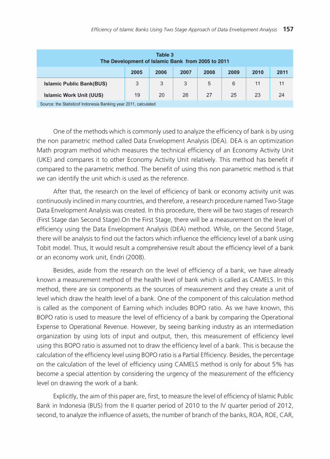
157Efficiency of Islamic Banks Using Two Stage Approach of Data Envelopment Analysis
One of the methods which is commonly used to analyze the efficiency of bank is by using the non parametric method called Data Envelopment Analysis (DEA). DEA is an optimization Math program method which measures the technical efficiency of an Economy Activity Unit (UKE) and compares it to other Economy Activity Unit relatively. This method has benefit if compared to the parametric method. The benefit of using this non parametric method is that we can identify the unit which is used as the reference.
After that, the research on the level of efficiency of bank or economy activity unit was continuously inclined in many countries, and therefore, a research procedure named Two-Stage Data Envelopment Analysis was created. In this procedure, there will be two stages of research (First Stage dan Second Stage).On the First Stage, there will be a measurement on the level of efficiency using the Data Envelopment Analysis (DEA) method. While, on the Second Stage, there will be analysis to find out the factors which influence the efficiency level of a bank using Tobit model. Thus, It would result a comprehensive result about the efficiency level of a bank or an economy work unit, Endri (2008).
Besides, aside from the research on the level of efficiency of a bank, we have already known a measurement method of the health level of bank which is called as CAMELS. In this method, there are six components as the sources of measurement and they create a unit of level which draw the health level of a bank. One of the component of this calculation method is called as the component of Earning which includes BOPO ratio. As we have known, this BOPO ratio is used to measure the level of efficiency of a bank by comparing the Operational Expense to Operational Revenue. However, by seeing banking industry as an intermediation organization by using lots of input and output, then, this measurement of efficiency level using this BOPO ratio is assumed not to draw the efficiency level of a bank. This is because the calculation of the efficiency level using BOPO ratio is a Partial Efficiency. Besides, the percentage on the calculation of the level of efficiency using CAMELS method is only for about 5% has become a special attention by considering the urgency of the measurement of the efficiency level on drawing the work of a bank.
Explicitly, the aim of this paper are, first, to measure the level of efficiency of Islamic Public Bank in Indonesia (BUS) from the II quarter period of 2010 to the IV quarter period of 2012, second, to analyze the influence of assets, the number of branch of the banks, ROA, ROE, CAR,
���������������������������������������������������������
���������������������������������������������������������������
���� ���� ���� ���� ���� ���� ����
�
��
�
��
�
��
�
��
�
��
��
��
��
��
������������������������
�����������������������
158 Bulletin of Monetary, Economics and Banking, October 2013
and NPF toward the efficiency level of Islamic Public Bank (BUS) in Indonesia from the II quarter period of 2010 to the IV quarter period of 2012, third, to analyze the comparison between the measurement method of efficiency level using Data Envelopment Analysis (DEA) and the measurement of the health of bank using CAELS, and fourth, to formulate a Policy Implication which can be given as the form of implication from the result of the measurement using the method of Data Envelopment Analysis (DEA).
II. THEORY
The analysis about the efficiency of an Economy or a Company Work Unit was always about how to result a maximum output with certain number of input, Farrell (1957). In describing a condition of the achievement of efficiency in a company Farrell (1957) illustrated his idea through a simple example by a case of a company using two inputs ( x1and x2) to produce a singular output (q) by an assumption of constant return to scale (CRS). By using the line of isoquant from a company with a fully efficient firm, represented by the curve of SS’in picture1, then, a calculation of technical efficiency could be conducted. If a company had used certain number of inputs which were shown by point P to produce an output unit, then, the technical inefficiency of that company would be represented by the distance of QP which was the total of all inputs which proportionally can decrease and be decreased without causing the decline of the output resulted. This indicator was commonly written mathematically in percentage as the ratio of QP/0P, as the description of the percentage of the input that can be decreased. In general, the level of technical efficiency/TE in the company was measured by the score of ratio:
TE = 0Q/0P
That equation would be the same with the equation of 1-QP/0P, in which the score was ranged from zero to one, and therefore, it resulted the indicator of the degree of technical efficiency from that company. The score of 1 implicated that the company had reached the fully efficient firm. For example, the point of Q had reached the technical efficiency because it was in the position of the curve of efficient isoquant.
If the ratio of the price of input (in picture 1) presented by the line AA’ was also known, then allocative efficiency of production could be calculated. The level of allocative efficiency/AE of a company which oriented from the point of P could be defined as the ratio of:
AE = 0R/0Q
In which the distance of RQ showed the decrease of the production cost which could be gained if the level of production was on point Q’ which was allocatively and technically efficient, and it was different from Q point which was technical efficient but allocatively inefficient.
The total economic efficiency could be defined as the ratio of:
EE = 0R/0P

159Efficiency of Islamic Banks Using Two Stage Approach of Data Envelopment Analysis
In which the distance from the point of R to point of P could be interpreted with the term of cost reduction. it showed that the product which was technically and allocatively efficient showed the achievement of the economic efficiency comprehensively.
TE x AE = (0Q/0P) x (0R/0Q) = (0R/0P) = EE
Picture 1. TheTechnical and Allocative Efficiency
�
�
�
��
�
�
����
��
�
���������������������
In describing the illustration drawn by Farrel, thus, a programming model to measure the relative efficiency level called as Data Envelopment Analysis (DEA) was formulated by Charnes, Cooper, and Rhodes in 1978, (Charnes el al. 1978). The DEA modeling aimed to measure the relative efficiency level of a company compare to the same type of company. Some research on the efficiency of a company, especially on the banking industry had been numerously used all over the world. Supachet Chansarn (2008) conducted a research about level of efficiency of commercial bank in Thailand along 2003-2006. The result showed that the level of efficiency of the commercial bank in Thailand was stable and was very high with the average of 90% for every year along the period of the research. While on the research conducted by Anne (2010) it showed that the average score of efficiency score of banking sector was not more than 40% along the period of 1997-2009. Based on that research, it was seen that there was a different of the result of the score of efficiency between the banking sector in Thailand and in Kenya which described the condition of those two countries’ banking sector.
III. RESEARCH METHODOLOGY
3.1. Object and Research Variable
The objects of this research included ten Islamic Public Bank in Indonesia, such as Bank Muamalat Indonesia, Bank Syariah Mandiri, Bank Syariah Mega Indonesia, Bank Bukopin

160 Bulletin of Monetary, Economics and Banking, October 2013
Syariah, Bank Rakyat Indonesia Syariah, Bank Panin Syariah, Bank Jabar Banten Syariah, Bank Victoria Syariah, Bank Negara Indonesia Syariah, and Bank Central Asia Syariah along the Second Quarter period of 2010 until the Fourth Quarter period of 2012. The using these ten Islamic Public Banks (BUS) in this research by deleting Bank Maybank Syariah Indonesia which was established in the Fourth Quarter of 2010 as the object of study because of the abnormal spread of data on the analysis of Second Stage using Tobit model. The data used in this research was included into the type of quantitative data and based on the source of data; this research used the secondary data.
In this research, the selection of the input and output variable to measure the level of efficiency using the method of Data Envelopment Analysis (DEA) on the First Stage used the intermediation approach as what have been used by Efendic (2009: 1-13) and Rahmat Hidayat (2011: 1-19). The input variables (I) which were used in this research included the third-party fund or DPK (I1), total assets (I2), and labor cost (I3). Besides, the output variables (O) used were financing (O1) and Operational Income (O2).
On the second stage, the dependent variable analyzed by using the model of Tobit in analyzing the factors influences the level of efficiency of an Islamic Public Bank in Indonesia was the result score of the measurement of DEA. Besides the independent variable which were used were assets (X1), the number of the branch of the banks (X2), ROA (X3), ROE (X4),CAR (X5), and NPF (X6).
3.2. Data Envelopment Analysis (DEA)
Data Envelopment Analysis is a method of non parametric which is used to measure the level of efficiency of an Economy work Unit (UKE). Besides, DEA is a method used to evaluate the efficiency of a decision maker unit (work unit) which is responsible for the using of some inputs to get the targeted output. In special, DEA is the improvement of a linear technical programming which has the function of purpose and the function of obstacle. Below is the general equation on the method of Data Envelopment Analysis (DEA).
∑∑
=
== n
j jsjs
m
i isiss
yu
yuh
1
1
In which hs showed the technical efficiency of banks; uis show the weight of the resulted output i; yis is the weight of the produced input i; vjs is the weight of the input j; and xjs = the number of input j given by bank s.
In this case, it also finds the score for u and v, as the maximum efficiency measurement of hs. With the purpose for the obstacle that all measurement of the efficiency must be less

161Efficiency of Islamic Banks Using Two Stage Approach of Data Envelopment Analysis
than or the same as one, one of the problems of formulations of this ratio is that this has many infinite solutions. To avoid this, then, we can determine the obstacle which will specify and easier the next process by using the computation technique which always develop all times. The function of that obstacle is below:
Nryu
yun
j jsjs
m
i isis ...,,2,1;11
1 =≤∑∑
=
= and 0, ≥ji yu
In which N shows the number of bank in the samples. The first inequality shows the ratio of efficiency for other company which is not more than 1, while for the second inequality is positive in value/score. The value/score of ratio will vary between 0 and 1. A bank can be said as efficient if the ratio score is close to 1 or 100 percent, and in contrast, if it is close to 0, it shows that the efficiency of a bank gets lower. On DEA, every bank can determine its own weighted and guarantee that the chosen weighted will result the best performance.
Related to the input and output used in the measurement of the efficiency, there are three approaches used, such as the approach of assets, production and intermediation. In this research, it used intermediation approach, because according to Hadad (2003: 3), he explained that the real activity of a bank organization with its function was as the organization of intermediation. Besides, It had been numerously used in research to measure the level of efficiency of banking in all over world.
Besides determining the input and output of the research, on the measurement of the efficiency level, there are two models used to analyze the efficiency of an Economy Work Unit (UKE). The first developed model was model with assumption of constant return to scale (CRS) or commonly called as the model of CCR (Charnes-Cooper-Rhodes). In the model of constant return to scale, every UKE will be compared to the whole UKE in the samples with assumption that the internal and external conditions of the Economy Work Unit are the same. According to Charnes, Cooper, and Rhodes, this model can show the technical efficiency comprehensively or the show the score of the profit efficiency for every Economy Work Unit.
In the model of CRS, there is a general Math model that has been explained on the general equation above. In that equation, it is explained that the value or score of technical efficiency can be gained through the comparison between the output ratios toward its input ratio. Further more, in that equation, it is explained that the score of measurement of efficiency score is limited in the range score of 0 until 1 and the score weight must be positive. Through that equation, it can be concluded that a Bank is stated to be efficient if it has the ratio score closes to 1 or 100 percent, in contrast, if the score is close to 0, it shows that the bank efficiency gets lower. Below is the equation of the model of CCR:

162 Bulletin of Monetary, Economics and Banking, October 2013
0,
1
,...,1;0.
.
1
11
1
≥
=
=≤−
=
∑∑∑
∑
=
==
=
ji
m
j jsj
m
j jrjm
i iri
m
i isis
vu
xv
Nrxvyust
yuhMax
In that equation, it is explained that the function of purpose of that equation is to maximize the output by the function of obstacle, in which the input score is the same as one thus, the output value/score which is lessen by its output value/score will be less than or the same as 0. This means that all banks will be in the position or below the level of technical efficiency.
While the second model developed in the level of the measurement of efficiency is model by assumption of variable return to scale (VRS) or usually called as the model of BCC (Bankers-Charnes-Cooper). In this model, it is assumed that the condition of all Economy Work Unit are not the same or it can be said that not all Economy Work Unit operate optimally. The inelastic competition, the financial burden, etc can cause the company cannot operate optimally. The Math model with the approach of VRS can be modified from the model with CRS approach and still can compass on the general Math model of DEA as the equation in measuring the level of technical efficiency. By adding the obstacle of convexity constraint into the equation, so that the Math formula becomes:
0,
1
,...,1;0.
.
1
11
01
≥
=
=≤−
+=
∑∑∑
∑
=
==
=
ji
m
j jsj
m
j jrjm
i iri
m
i isis
vu
xv
Nrxvyust
UyuhMax
In which U0 is a piece that can be positive or negative in value/score.
In this research, it used model with assumption of constant return to scale (CRS) or called as model of CCR (Charnes-Cooper-Rhodes). This model was chosen based on the research conducted by Suseno (2008: 35-55) about the unavailability of relation between the efficiency level of Islamic bank (study on ten Islamic banks) and its production scale. In that research, it was explained that the economy scale in banking industry did not occur based on the company scale because of the function one bank has been integrated with other banks. Therefore, the economy scale has moved from the company to functional. In Indonesia, this can be observed from the phenomenon of the using of collective ATM machine, collective credit card service or

163Efficiency of Islamic Banks Using Two Stage Approach of Data Envelopment Analysis
collective marketing, so that the efficiency level was not seen in the company scale but possibly seen in the scale of functional of national banking industry (not merely in the industry of Islamic banking). In this research, it also used efficiency by the approach which oriented to the output, this was because, in the end, the purpose of an economy Work Unit was to get the maximum benefit by optimizing its resources.
3.3. Tobit Model
In this stage, it will conduct the analysis on factors influence the efficiency level. it gained the efficiency value or score on the first stage by using the method of DEA, thus, that score will be analyzed with some environment variables to find out the relation and the characteristic of relation between those variables toward the second stage. Therefore, these two stages in this research was called as Two-Stage Data Envelopment Analysis. In analyzing the factors influenced the level of efficiency, it used model of Tobit.
The calculation of Tobit was stated by James Tobin in 1958 when he analyzed the expense of households in the USA to buy cars. The expense for car in some households became zero (because that household did not buy car), and the this thing influence toward the result of the regression analysis. He found that if still using OLS, the calculation of the parameter will tend to be close to zero and became insignificant, or if became significant, the score experienced a bias (too big or too low) and became inconsistent (if there were new data, the result would not be the same or did not fit with the previous result).
The method of Tobit assumed that independent variables is unlimited in score (non-censured); only the dependent variables which were censured; all variables (both independent and dependent) was measured correctly; there was no autocorrelation; no heteroscedascity; no perfect multicolinearity; and the mathematic model used became precise in the using of analysis regression method for social and economic field, there were many data structure in which the response variable had the score of zero for some observation parts, while for other parts of observation had certain score which were vary. The data structure like this was named as censored data, Endri (2008).
3.4. The Method of CAELS Health Measurement and Method of Independent Sample T Test of Wilcoxon Signed Ranks Test
In this research, besides describing the level of efficiency toward the Islamic Public Bank through the procedure of Two-Stage Data Envelopment Analysis, there was also comparison between the results of the measurement of efficiency level of DEA with the result of the measurement of health by CAELS method. The reason of the using of CAELS method without using the component of “M” which was known as CAMELS was because in CAMELS method in Indonesia, there was different treatment for the score of financial factor which united became

164 Bulletin of Monetary, Economics and Banking, October 2013
CAELS and management factor. Besides, to make the result of DEA method could be integrated on CAELS method, thus, the result of the method of DEA was divided into 5 categories, which are category “1”: 100% (very efficient), category “2”:80% to 99.99% (Efficient); category “3”:60% to 79.99% (Efficient enough); category “4”:40% to 59.99% (inefficient); and category “5”:0% to 39.9% (Very inefficient).
Meanwhile, to analyze the comparison between the result of using DEA method and the result of CAELS method, the independent sample T test of Wilcoxon signed rank test is conducted. The Method of Independent sample T test of Wilcoxon Signed Ranks Test is a non parametric test that can be used if the distribution of the data is abnormal which is used to test whether there is any different or not between those two pairs of sample group Priyatno (2011: 318). Next, the result of the independent t test between the method of DEA and CAELS will be analyzed and illustrated into some modification method of CAELS + DEA in the form of mapping.
IV. RESULT AND DISCUSSION
4.1. The Result of the Measurement of the Level of Efficiency of Islamic Public Bank (BUS) from the II Quarter Period of 2010 to the IV Quarter Period of 2012 (First Stage)
In this discussion, there would be shown the level of efficiency of 10 (ten) Islamic Public Banks based on the method of Data Envelopment Analysis (DEA) along the IV quarter period of 2010 until the IV quarter period of 2012, and it would show the level of the average efficiency which were reached by each Islamic Public Bank along that period of time. The data on the input and output variables for measuring the efficiency level were taken from the publication report of the Islamic Public Bank in Indonesia. As what have been explained before, DEA method presented the result of the measurement of the level of efficiency in the form of efficiency score with range 1-100. Score100 presented the Islamic Public Bank which optimized its resources. In contrast, if the score was below 100, it mean that the Islamic Public Bank was said to be inefficient to optimize its resources and had yet to perform its function as an optimum intermediation organization. In this research, the result of measurement using the method of DEA would be presented in some graphs presenting the achievement of the average level efficiency of each Islamic Public Bank within quarter period, and the achievement of efficiency level of the Islamic Public Bank in comprehensive way.

165Efficiency of Islamic Banks Using Two Stage Approach of Data Envelopment Analysis
Picture 2. The Efficiencyof Ten Islamic Public Bank from the II Quarter period of 2010 to the IV Quarter Period of 2012
�������� ��������������������������� �������������������������� ����������������������������� ���������������������� ��������������������
�������������������������������������������������
���������������
� � � � � � � � � � �� ��
The result of the level of efficiency of the Islamic Public Bank in the II Quarter Period of 2010 until in the IV Quarter Period of 2012 showed a trend of fluctuation, there was no Islamic Public Bank (BUS) which had a stable efficiency score from every period of measurement. Besides, based on the result of measurement from that efficiency, it could be seen that there were some Islamic Public Bank which got the score of 100, or it could be translated that these banks had been able to optimize their all resources and were categorized as the efficient bank. And the bank which were categorized as the efficient banks were Bank Muamalat Indonesia and Bank BNI Syariah in the I Quarter, Bank Muamalat Indonesia and Bank Syariah Mega Indonesia in the III Quarter, Bank Muamalat Indonesia and Bank Jabar Banten Syariah in the IV Quarter, Bank Panin Syariah in the VI Quarter, Bank BRI Syariah, Bank Victoria Syariah, and Bank Panin Syariah in the VII Quarter, Bank Muamalat Indonesia, Bank BRI Syariah, and Bank Panin Syariah in the VIII Quarter, Bank Panin Syariah in the X Quarter, Bank Syariah Mega Indonesia and Bank Panin Syariah in the XI Quarter. Meanwhile, the other Islamic Public Banks were categorized as inefficient or it could be said that they had yet to optimize their resources.
After presenting the graph of the level of efficiency of the Islamic Public Bank along the II Quarter period of 2010 until the IV Quarter period of 2012, we would see the achievement of the average of the level of efficiency of every Islamic Public Bank along the period of time of this research. Based on Picture 2, it could be seen that the Islamic Public Bank which had been established earlier such as Bank Muamalat Indonesia and Bank Syariah Mandiri had better average level of efficiency than other newly established Islamic Public Banks such as Bank Victoria, Bank BNI Syariah, and Bank BCA Syariah. However, just like what have been stated before that there was an Islamic Public Bank which was newly established such as Bank Panin

166 Bulletin of Monetary, Economics and Banking, October 2013
Syariah which became the bank with efficiency score of 100 within 5 times and this condition could not be reached by other banks during the research observation of time. This also occurred in the achievement of Bank BRI Syariah and Bank Bukopin Syariah which had good level of efficiency, even though they were new in the industry of Islamic banking in Indonesia.
Based on that result above, then, comprehensively, the development of the level of efficiency of Islamic Public Bank had the fluctuation trend because of the efficiency level of the bank in individual was also fluctuate as what had been presented in Picture 1.During the period of study, the highest score of efficiency of the Islamic Public Bank was reached in the IV Quarter period of 2011 with the score of 91.89 and the lowest score of efficiency occurred in II Quarter of 2011 with score of 78,46. Through this result, it could be concluded that the Islamic Public Bank in Indonesia were still categorized as inefficiency or they had yet to optimize their resources. That condition was appropriate with the research conducted by Endri (2008).
Picture 3. The Efficiency of Islamic Public Bank (the average score within the II Quarter period of 2010 –IV/ 2012)
���
��
��
��
��
��
��
��
��
��
�
����� ����������
����� ����� �����
�����
����� ����������
������
����
���
�������
�������
������
�������
�������
���
�������
��������
�����
�������
������
���
�������
������
�����
����������
������
�����
������������
�����
��������
�������
������
���
�������
������
���

167Efficiency of Islamic Banks Using Two Stage Approach of Data Envelopment Analysis
In this research, it will present the comparison with other similar research. By the different time of research, the two result of measurement using DEA method of the Islamic Public Bank will be the roadmap that shows the pattern of the result of efficiency of those banks from time to time. In picture 4, it shows the result of measurement in this research and the result of measurement conducted by shafitranata (2011: 47-48). The different between these two researches were in the time and the number of Islamic Public Bank which were observed. This research used 10 (ten) Islamic Public Bank as the object of the research within period of 2010 until 2012 and the research conducted by shafitranata used 3 (three) Islamic Public Bank with time of research was from 2007 to 2010. In Picture 4, it will show the annual data.
In these two researches, there was the presentation of the result of measurement of efficiency level within period of 2007 – 2012. Along that period of time, it could be seen that there was positive trend of efficiency of the Islamic Public Bank in Indonesia. Even though, the graph experienced a decline in 2008, after that, the graph of efficiency showed an increase.Moreover, there was a difference in the result of measurement in 2010. Still, that condition could be understood because during that period of time, there was the different in the number of the banks which were observed; in which this research used 10 (ten) Islamic Public Bank as the object of the research and shafitranata used 3 (three) Islamic Public Bank. Therefore, with the ranger of result of the research which was only 5,95in 2010, it could be concluded that comprehensively, there was a correlation of the result of the efficiency measurement from those two research.
Picture 4. The Efficiency of all Islamic Public Bank (the average score within the II Quarter period of 2010 –IV/ 2012)
��
��
��
��
��
���� �� �� �� �� ���� �� �� ����
���� ���� ����
����������
�����
�����
�����
�����
�����
�����
�����
�����
�����

168 Bulletin of Monetary, Economics and Banking, October 2013
4.2. The Result Analysis of Factors which Influence the Level of Efficiency of Islamic Public in the IV Quarter period of 2010 – in the IV Quarter period of 2012 (Second Stage)
On the next stage of this research, there will be an analysis on factors which influenced the efficiency level of Islamic Public Bank using Tobit model so that the whole procedure in this research is called Two-Stage Data Envelopment Analysis. In the analysis of Tobit model in this research, it used a package of software Eviews 7.2. The result of the analysis of Tobit model was used to conclude the factors which influence the efficiency level of the Islamic Public Bank. Below is the result analysis using Tobit model.
Picture 5. The Roadmapof theEfficiency of Islamic Public Bank from 2007 to 2012
�����
�����
�����
�����
����� ����� �����
���� ���� ���� ���� ���� ����
��� ����
�������������������������������������������
�������� ����������� ���������� ����������� �����
� �������� �������� �������� ������
���� �������� �������� �������� ������
������ ��������� �������� ��������� ������
��� �������� �������� �������� ������
��� �������� �������� �������� ������
��� ��������� �������� ��������� ������
��� ��������� �������� ��������� ������
Based on the result analysis on Table 4, it could be seen that there were some variables which gave positive and negative impacts. However, not all variables gave significant influence or it could be said that some variables did not give real influence. Thus, by using this Tobit model,

169Efficiency of Islamic Banks Using Two Stage Approach of Data Envelopment Analysis
we could see that assets variable had a positive influence and significant toward the efficiency of Islamic Public Bank. That condition was because by having lots of assets, a company could run more freely its operational activities and could achieve its optimum resources. Besides, a bank with many assets automatically would be easier to adopt new technology which could increase the profit and decrease the management cost. This result was suitable with the research conducted byIsmail, Rahim, and Majid (2009: 5).
Whereas the variable of branch of the bank had negative and significant influence or in other words the more branches of the bank the more inefficient the bank to control its resources. That condition was because the Islamic Public Bank in Indonesia had yet to achieve economies of scale and the addition of the number of branch of the bank would only increase the cost expended by that bank.This result of the research was the same as the research conducted by Jackson and Fethi (2000: 18).
On the variables ROA and ROE which represented the profitability level of a bank there were positive and significant influences. This was because a Bank that could create bigger profit could be indicated as an efficient bank. This result was appropriate with the research conducted by Gupta, Doshit, and Chinubhai (2008: 10).
On variabel NPF which showed the ratio of non-performing loan which occurred in a bank had negative and significant influence. This was because the higher the ratio of the ratio of non-performing loan in a bank automatically would disturb the operational activity of a bank, especially in on the side of liquidity of that bank. Therefore, that caused a bank to be inefficient on managing its all resources. This result of the research was appropriate with the research conducted by Ismail, Rahim, and Majid (2009: 5).
On CAR variable which presented the capability of capital of a bank in covering the risk, showed that there was negative influence between that variable and the level of efficiency of Islamic Public Bank. In this variable, there was the role of government on determining the level quantity of CAR that must be fulfilled by a bank, which was for about 8%. The result of this research showed that the lower level of CAR of an Islamic Public Bank, the higher efficiency of an Islamic Public or in other words, there were negative and significant influence between the level of CAR and the level of efficiency of Islamic public Bank. That condition probably reflected the risk-return trade-off. This occurred because if the tendency of the society prefer to choose a bank with a lower risk to a bank with higher risk but more productive.This result of research was in a line with the research conducted by Jackson and Fethi (2000 : 18).
4.3. The Result Analysis of the Independent Sample T Test between DEA Method and CAELS Method
On this stage, there would be analysis of comparison between the method of efficiency DEA and the method of measurement of work performance CAELS along the period of time

170 Bulletin of Monetary, Economics and Banking, October 2013
of the research by using the method of the test of independent sample t test of Wilcoxon Signed Rank Test. The purpose of this analysis was as the evaluation tool toward the method of measurement of work performance CAELS which was released by Bank of Indonesia and as the matter of concerns to Bank of Indonesia to integrate the calculation of the method of efficiency DEA in the model of measurement of work performance CAELS which would be shown in the next stage.
On Table 5, it could be seen that the result of analysis of this test showed that there was significant different between the result of these two methods.This could be seen on Asymp. Sig. (2-tailed) which showed the score below 0.05.
��������������������������������������������������������������������������������������������������
���������
� ������
��������������������� ����
From that result, there were 2 (two) things that could be explained from the result of that test above. First, on method of CAELS, weight given on the measurement of efficiency using the ratio of BOPO was only for about 5%. This was, of course, was imbalance with the meaning of efficiency in a company or in this case was Islamic Public Bank. This was because efficiency was one of the important indicators which presented the work performance of a bank. A bank is categorized as efficient if it can optimize its all resources, can apply strategy to maximum its profit or to minimum its cost expended. Furthermore, a bank is categorized as efficient because it can give more benefit to its customer either the customer as depositor or as funder. This is because the bank can optimum its customer funds and maximum its role as the intermediation organization. Thus the justification of weight given is imbalance with other components in the model of measurement of CAELS.
Second, the attention was pointed out to the ratio of BOPO which became the indicator of efficiency on the model of measurement of the work performance of CAELS method. The BOPO ratio that only compared Operational Expense and Operational Revenue could not be the indicator to present the efficiency of a bank comprehensively. This was because by seeing the business of banking as the production process which included input and output, then, by this meaning, it meant that there would be combinations from many inputs that would result output optimally and this condition could not be found on ratio BOPO which only compared operational expense and operational revenue. Meanwhile, on DEA method which was called

171Efficiency of Islamic Banks Using Two Stage Approach of Data Envelopment Analysis
as frontier approach, it would result an optimum point in which by the minimum input could produce maximum output by using the combination of input and output. With that strength, then the measurement of the efficiency level using DEA was assumed as the method which drew the banking business in ideal way. Or in other words, it could be said that the calculation of efficiency level using ratio BOPO was assumed as Partial Efficiency, meanwhile the calculation of the level of efficiency using the method of Data Envelopment Analysis was ensured as Comprehensive Efficiency.
According to the things above, it could said that the measurement by CAELS method had yet to draw the work performance of a bank in a comprehensive way. Therefore, on the last stage, there would be the illustration of the model of the measurement of the work performance which integrated the result of measurement by using DEA method in CAELS method.
4.4. The Mapping Result of the Modification of CAELS + DEA Method
After conducting the analysis on the comparison between the method of efficiency measurement using DEA by the method of test of different of wilcoxon signed rank test on the previous stage, in this stage, there would be illustration of the result of the modification of CAELS method by integrating the result of DEA method by a mapping graph showing the result of measurement before and after the integration of DEA method into the method of measurement of work performance CAELS.
Before conducting the mapping, there would be drawn a method of the measurement of work performance CAELS with 3 (three) modifications on the weighted and the process of integrating DEA method into CAELS method in the form of table.
����������������������������������������������
��������� ������� ����������
������� ������� ���
������������� ������� ���
������� �������� ��
������� ��
��������� ������� ���
����������� ������ ��
����� ����
���������������������������������������
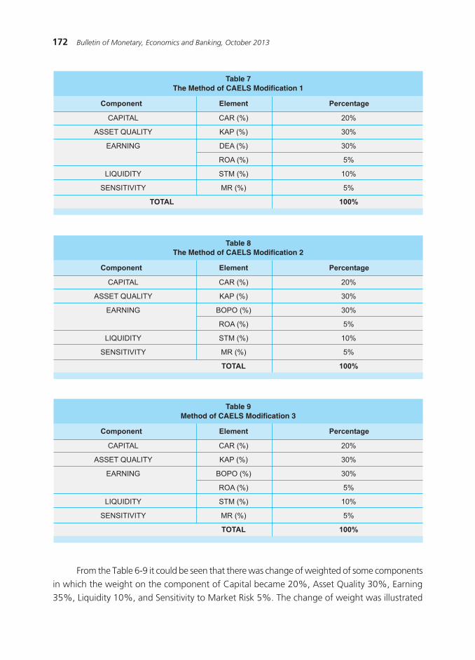
172 Bulletin of Monetary, Economics and Banking, October 2013
�����������������������������������������
��������� ������� ����������
������� ������� ���
������������� ������� ���
������� ������� ���
������� ��
��������� ������� ���
����������� ������ ��
����� ����
�����������������������������������������
��������� ������� ����������
������� ������� ���
������������� ������� ���
������� �������� ���
������� ��
��������� ������� ���
����������� ������ ��
����� ����
�������������������������������������
��������� ������� ����������
������� ������� ���
������������� ������� ���
������� �������� ���
������� ��
��������� ������� ���
����������� ������ ��
����� ����
From the Table 6-9 it could be seen that there was change of weighted of some components in which the weight on the component of Capital became 20%, Asset Quality 30%, Earning 35%, Liquidity 10%, and Sensitivity to Market Risk 5%. The change of weight was illustrated

173Efficiency of Islamic Banks Using Two Stage Approach of Data Envelopment Analysis
on CAELS modification 1 and CAELS modification 3. Meanwhile on CAELS modification 2, the weight is equalized to the formula of the method of CAELS before modification.
The change on the weight conducted based on the characteristic of the method CAELS which was flexible and did not based on the basic rule applied in all countries. Based on the discussion in the library study in this research, the amount of weight on each component was conducted based on justification of the regulator from every country. Therefore, the modification of the weight conducted in this research could be the thing that legalized so that the modification done in this research could be one of the considerations for Bank of Indonesia as the regulator in measuring the work performance of a bank.
Besides the change on the weight, the change was also conducted by changing the ratio of BOPO by the method of efficiency DEA. This was conducted on CAELS modification 1 and CAELS modification 3. Meanwhile on CAELS modification 2 still used ratio BOPO but the weight was changed. Thus, comprehensively, there would be illustration about 3 (three) modification from the method CAELS and method CAELS before modification.
After drawing the illustration of the modification of the method CAELS, then, after that, there would be mapping in the form of graph to see the result from the method CAELS before and after modification. As known in the method of CAELS, the work performance of a bank was divided into 5 (five) categories, which were: “1” (Very Good), “2” (Good), “3” (Quite Good), “4” (Weak), and “5” (Very Weak).
Picture 6. The Graph of Mapping of the Method of CAELS and Modification method of CAELS + DEA
��
��
�
��
�� ��
��
��
� � � � � � � � � � � �
���
��
��
��
��
������������ ���� ���������� ����� ������������
�����
�����������
�����������
�����������
On Picture 6, there was mapping graph showing the result of measurement of the health of bank by spread of each categories on method CAELS and 3 (three) methods modification CAELS + DEA. Through those 4 (four) graphs, the difference of the result measurement of the

174 Bulletin of Monetary, Economics and Banking, October 2013
health of the bank by the spread on every category seen on the modification of CAELS + DEA 1 and modification CAELS + DEA 2. Whereas the result of the measurement of the health of the bank with the same spread on every category could be seen through graph of CAELS before modification and modification CAELS + DEA 3.
By referring to the result of those 4 (four) graphs, it was found that by the change of the portion of the weight of some components as well as by the change of the ratio of BOPO by the method of efficiency DEA (modification CAELS + DEA 1) would change some result of measurement on the level of health of the bank if compared to the result of the measurement of the health of the bank before the modification. Meanwhile, if we did not change the weight on some components on method CAELS (modification CAELS + DEA 3), thus the result gained was the same like the result before the modification on CAELS method, even though we have changed the ratio of BOPO with the method efficiency of DEA method. Different thing happened if we made the change on weight without changing the ratio of BOPO with the method of efficiency DEA (modification CAELS + DEA 2), and then, it would be seen the result of the measurement of the health of the bank with the number of the bank which were on category “1” (very good) increased fast if compared to 3 (three) other graphs.
Therefore, by having that mapping. We could say that the ratio of BOPO could not map the efficiency of a bank as a whole. As what had been explained on the previous analysis, the ratio of BOPO was only a simplification of the measurement of efficiency of bank. Or in other words, the calculation using ratio of BOPO was assumed to be Partial Efficiency. Moreover, the change on the weight would change the result of the measurement of the health of bank. With a main focus on earning component with efficiency measurement inside, thus, there should be adaptation by changing the weight on some components in order to increase the portion of the weight on the efficiency measurement. This was because of the imbalanced of the portion of the weight of the earning component, especially on the measurement of efficiency which was only given weight for about 5%. With the urgency of the function of a work performance of a bank, such as the indicator of the achievement of an optimum work performance by optimizing its all resources as well the ability to maintain its survival, then, the increased of the weight was needed to be consideration.Then, the last thing as the focus on the modification of CAELS was to change the ratio of BOPO with the method of efficiency DEA. Because based on the mapping applied, it could be proven that the method efficiency of DEA could give the illustration of the efficiency of a bank as a whole so that it could filter the result measurement of the health of the bank through the change of the number of the bank on some categories.Therefore, policy implication offered and expected to be consideration for Bank of Indonesia as the regulator was pointed out to the modification of the method of CAELS + DEA 1.
175Efficiency of Islamic Banks Using Two Stage Approach of Data Envelopment Analysis
V. CONCLUSION
This research gave some finding results, First, in general the efficiency level of 10 (ten) Islamic Public Bank had trend to fluctuate during the period of time of the research. Individually, Bank Muamalat Indonesia had the highest of the average efficiency level score of 93,82 and Bank Victoria Syariah had the lowest of the average efficiency score of 72.12.
Second, by the model application of Tobit, it was concluded that variables of branch bank, Non-Performing Financing (NPF), and Capital Adequacy Ratio (CAR) had negative influence and significant toward the efficiency level of the bank. Meanwhile on the variables Assets and Return On Asset (ROA) Return On Equity (ROE) had the positive influence and significant.
Third, the comparison between the measurement of efficiency using DEA method and the measurement of performance of work using CAELS method (through the independent sample t test of Wilcoxon Signed Rank Tests) showed differences between those two. Therefore, as the alternative which was presented in this research was by integrating the method of efficiency of DEA as the substitution of ratio BOPO as the indicator in measuring the efficiency. This could be proven that the result of mapping in which the method of CAELS for the measurement of health which had been integrated with DEA resulted a change on the result of the measurement of the health of the bank by decreasing the number of banks in category “1” (Very Good). This was because some banks on that category had low score of level of efficiency, and, of course, this thing could happen by improving the weight portion on the earning component in which in this earning component, there was the result of the measurement of efficiency of DEA method.
The findings above had some policy consequences that point out a detail attention towards factors that influence to the efficiency level. Besides, the method of DEA with the adjustment that had been illustrated in this research could be the alternative method for measuring the health of the bank.

176 Bulletin of Monetary, Economics and Banking, October 2013
rEfErEncEs
Charnes, A., Cooper, W.W., Rhodes, E. 1978. Measuring the Efficiency of Desicion Making Units. European Journal of Operational Research, 429-444.
Chansarn, Supachet. 2008. The Relative Efficiency of Commercial Banks in Thailand . International
Research Journal of Finance and Economics, 53-68.
Efendic, Velid. 2009. Efficiency of Banking Sector of Bosnia-Herzegovina with Special Reference to Relative Efficiency of Existing Islamic Bank. International Conference on Islamic Economics
and Finance, 1-13.
Endri. 2008. Efisiensi Teknis Perbankan Syariah di Indonesia. Finance and Banking Journal, Vol. 10.
Farrell. 1957. The Measurment of Productivity Efficiency. Journal of the Royal Statistical Society, 254
Hadad, Muliaman D. dkk. 2003. Analisis Efisiensi Industri Perbankan Indonesia: Penggunaan Metode NonParametrik Data Envelopment Analysis (DEA). Working Paper Series Bank
Indonesia, 3.
Hidayat H. Rahmat. 2011. Kajian Efisiensi Perbankan Syariah Di Indonesia (Pendekatan Data Envelopment Analysis). Media Riset Bisnis & Manajemen, 1-19.
Ismail, Farhana, Rossazana Ab. Rahim, dan M. Shabri Abd. Majid. 2009. Determinant of Efficiency in Malaysian Banking Sector. Skripsi S1 Universiti Malaysia Sarawak, 5.
Jackson, Peter .M dan Meryem Duygun Fethi. 2000. Evaluating the Technical Efficiency of Turkish Commercial Bank: An Application of DEA and Tobit Analysis. University of Leicester, 18.
Kamau, Anne W. 2011. Intermedation Efficiency and Productivity of The Banking Sector in Kenya. Interdisciplinary Journal of Reseacrh and Business, 12-26
Omprakash K. Gupta, Yogesh Doshit, dan Aneesh Chinubhai. 2008. Dynamics of Productive Efficiency of India Banks. International Journal of Operations Research, 10.
Priyatno, Duwi. 2011. Buku Saku SPSS Analisis Statistik Data Lebih Cepat, Efisien, dan Akurat. Yogyakarta: PT. Buku Seru, 318.
Shafitranata. 2011. Tingkat Efiseiensi Bank Umum Syariah Menggunakan Metode Data Envelopment Analysis (DEA). Dalam Forum Riset Perbankan Syariah, ed. Bahan-Bahan
Terpilih Dan Hasil Riset Terbaik. Bandung: Universitas Padjajaran, 47-48.
Suseno, Priyonggo. 2008. Analisis Efisiensi dan Skala Ekonomi pada Industri Perbankan Syariah di Indonesia. Pusat Pengkajian dan Pengembangan Ekonomi Islam,Vol. 2, 35-55.

177
WRITING GUIDANCE
1. The paper should be original and should not violate any copyrights. The submitted paper
should have never been published or not being submitted to other publisher. The copyright
of the published paper is retained to the author.
2. The Bulletin of Monetary Economics and Banking provide a financial incentive between IDR
5,000,000.
3. The paper should be submitted in two formats (i) Microsoft Word (*.doc) and (ii) portable
digital file (*.PDF). These files should be sent to the following mail address:
[email protected] and Cc to: [email protected]
You may save your files in CD and send it to the following Editorial Address:
Bulletin of Monetary econoMics and Banking
department of economic research and Monetary Policy-Bank indonesia
Building syafruddin Prawiranegara, 20th floor
Ji. M. H. thamrin no. 2 central Jakarta, indonesia
Ph. +62-21-2310108 / 2310408 ext. 4119, fax: 62-21-3800394
4. To avoid missing fonts or other compatibility issues, any special characters or mathematical
expression (equations, symbols, matrix, etc.) must be written using Microsoft Equation.
5. The submitted paper should contain (i) an abstract of maximum one page A4, (ii) keywords
and (iii) JEL classification code. See the JEL code at http://www.aeaweb.org/journal/jel_class_
system.html.
6. The paper must contain the followings:
The background, the aim of the paper and its distinction to previous study
Theory and review of literatures
Methodology (quantitative methodology is preferred)
Result and analysis
Policy and further study implication
7. The citation should be in footnote and not in endnote.
8. The references must obey the following rule:

178 Bulletin of Monetary Economics and Banking, October 2010
a. Book:
Hanke John e. and arthur g. reitsch, (1940), Business Forecasting, Prentice-Hall, New
Jersey.
b. Article in journal:
rangazas, Peter. (2000) “Schooling and Economic Growth: A King-Rebelo Experiment
with Human Capital”, Journal of Monetary Economics, October, 46(2), page. 397-416.
c. Article in book edited by other people:
frankel, Jeffrey a. and andrew k., rose. (1995) “Empirical Research on Nominal
Exchange Rates”, in Gene Grossman and Kenneth Rogoff, eds.,”Handbook of International
Economics. Amsterdam: North-Holland, page. 397-416.
d. Working papers:
kremer, Michael and daniel, chen. (2000) “Income Distribution Dynamics with
Endogenous Fertility”. National Bureau of Economic Research (Cambridge, MA) Working
Paper No.7530.
e. Mimeo or unpublished work:
knowles, John. “Can Parental Decision Explain U.S. Income Inequality?”, Mimeo,
University of Pennsylvania, 1999.
f. Article from web or other electronic form:
summers, robert and alan W., Heston. (1997) “Penn World Table, Version 5.6”
http://pwt.econ.unpenn.edu/
g. Article in newspaper, magazine or equal periodicals:
Begley, sharon. (1993) “Killed by Kindness”, Newsweek, April 12, page. 50-56.
9. The paper should be submitted along with curriculum vitae complete with mail address and
phone number.