Coastal and Marine Geology / USGS Woods Hole Science Center

U.S. Geological Survey Open-File Report 2004-1443

2005

An Operation Manual for a Time-Series, Storm-Activated Suspended Sediment Sampler Deployed in the Coastal Ocean: Function, Maintenance, and Testing Procedures.

By Richard R. Rendigs and Michael H. Bothner

Contents Title Page Abstract Introduction Operational Software Summary The WTS-Tr and WTS-P Instruments - Getting Strarted Maintenance and Field Tests of the WTS-Tr Maintenance and Field Tests of the WTS-P Conclusions Bibliography Tables Figures Appendices

Any use of trade names is for descriptive purposes only and does not imply endorsement by the U.S. Government.

U.S. Department of Interior / U.S. Geological Survey / Coastal and Marine Geology / USGS Woods Hole Field Center

Abstract This manual describes the operation and testing procedures for two models of a multi-port suspended sediment sampler that are moored in the coastal ocean and that collect samples on a programmable time schedule that can be interrupted to collect during a storm. The ability to sense and collect samples before, during, and after the height of a storm is a unique feature of these instruments because it provides samples during conditions when it is difficult or impossible to sample from a surface ship. The sensors used to trigger storm sampling are a transmissometer or a pressure sensor. The purpose of such samples is to assess composition and concentration of sediment resuspended from the seafloor during storms and subsequently transported within the coastal system. Both light transmission and the standard deviation of pressure from surface waves correlate with the passage of major storms. The instruments successfully identified the onset of storms and collected samples before, during, and after the storm maximum as programmed. The accuracy of determining suspended matter concentrations collected by the sediment sampler has not been fully evaluated. Preliminary laboratory tests using a suspension of muddy sediment collected in a near-bottom sediment trap yielded excellent results. However in laboratory tests with different sediment types, the suspended matter concentrations determined with these samplers became less accurate with increasing average grain size. Future calibration work is necessary and should be conducted in a facility that ideally has a water depth of at least 30 feet to prevent cavitation of the pump that draws sea water through the filters. The test facility should also have the capability for adding suspended matter of known composition and concentration to a fixed volume of seawater that is well mixed. Introduction

The instrumentation described in this manual is designed to collect marine suspended sediment "in-situ" during a wide range of oceanic conditions. The unique feature of this instrument package is that it can collect samples during storms when collection by conventional methods from a surface vessel is impossible. Integrated sensors, which monitor either the pressure generated by surface wave height or the turbidity caused by resuspension of bottom sediment, identify storm conditions. The instrument also collects samples during non-storm conditions on the basis of a programmable time schedule. The goal of this instrument development is to improve our understanding of the fate and transport of sediments and associated contaminants. Both suspended and fine-grained bottom sediments have reactive surfaces that adsorb many contaminants from seawater. Knowledge about the concentration and composition of particulates under different hydrodynamic conditions is a critical component of sediment transport models This instrumentation has application to many coastal areas adjacent to metropolitan areas around the United States and the world where contaminants are of concern.

2

Massachusetts Bay has been the site of initial use because of an existing USGS program to provide basic scientific information to support management decisions related to the $4 billion upgrade to Boston's sewage treatment system. (Bothner and others, 2002; see also http://woodshole.er.usgs.gov/project-pages/bostonharbor/.) This report summarizes the operating procedures, maintenance, observations, and test results of two generations of suspended sediment samplers that were developed by McLane Laboratories of North Falmouth, Massachusetts, according to USGS specifications. The first version, referred to as WTS-Tr (McLane Research Laboratories model AT-WTS Mark 5-18), is a water transfer system activated on the basis of a transmissometer signal. The second unit, known as WTS-P (model WTS 6-24-47FH), is activated by changes in pressure caused by passing waves. Both sampling devices collect suspended matter by sequentially pumping a known volume of water through individual 47 mm diameter filters positioned along a valved manifold. The schedule of sampling events is selected using internal software to collect samples on a fixed time interval or in response to storm events according to a pre-determined threshold value from an external sensor or a combination of both. The WTS-Tr receives input from an external transmissometer, which generates a lower output voltage as the turbidity of the water increases. Mounted on a tripod 2 M above the seafloor at 30 M water depth, increasing turbidity is usually a result of storm-generated surface waves that can resuspend bottom sediment. As a storm progresses and the time averaged voltage readings fall below a pre-determined user-defined threshold, an algorithm contained in the WTS software initiates a sampling event representing the onset of the storm. The software continues to monitor changes in turbidity and samples again soon after a storm maximum is identified and again at the end of storm when the voltage is nearly back to pre-storm levels. At the end of the storm sampling sequence, the software will recalculate the scheduled sampling events for the remaining time of deployment unless the schedule is overridden by another storm event and a similar sampling sequence will be initiated. The WTS-P identifies storm events by using a piezoelectric pressure sensor (transducer) to monitor pressure changes caused by storm generated surface waves. Unlike the transmissometer sensor, the pressure sensor is not affected by biofouling. The software algorithm collects pressure readings over time and calculates the standard deviation of pressure (PSDEV) caused by surface waves generated by storm-induced winds. Surface waves and sediment resuspension are highly correlated (Bothner and others, 2002). The running time-averaged PSDEV trends are the basis for determining the first and subsequent sampling events during a storm cycle. If the averaged PSDEV values exceed a pre-determined threshold value, the software identifies the onset of a storm event and triggers a sampling sequence. The next sample is collected as the averaged PSDEV value begins to decrease immediately after the storm maximum. Three additional samples are collected after the maximum as the storm continues. After the storm has passed, the software will recalculate the remaining scheduled pump events in a manner similar to that of the WTS-Tr unless another storm event initiates an additional sampling sequence.

3

The two units have different styles of intake ports. The WTS-Tr has a separate port at the tip of each of the 18 individual filter holders. The WTS-P unit has a single entry port located on the manifold that is sequenced to each of the 23 filter holders. The WTS-P unit is designed to flush the entry port and connecting tube with filtered water before and after each sample is collected in order to minimize potential cross contamination between samples. Specifications and additional details for the WTS-P instrument type are available from the McLane Research Laboratories web site http://www.McLaneLabs.com, and McLane Research Laboratories User Manual, 1992. Operational Software Summary

The software for both WTS models may be accessed from a personal laptop computer (PC) within a DOS based environment through a standard RS232 serial port. A terminal emulation program allows the PC to communicate with the micro-controller on the WTS circuit board. The WTS-Tr utilizes a Tattletale Model 3 (TT3) data logger with volatile memory and controller. The McLane software is written in Basic language and the menu-driven format allows the user to program various instrument sensors and deployment parameters according to user-defined objectives. The deployment and recovery data are easily downloaded for record keeping and analysis. The WTS-P model uses an upgraded software package with a Tattletale Model 8 (TT8) data logger and controller supporting ANSI C and in-line assembly programming language. Storage and retrieval of deployment, recovery and data files are provided in non-volatile flash memory within the operating software. An E-Prom with RAM storage provides an additional backup for data recovery in the event of a system failure. The main menu for each instrument is organized with numbered options that control the various operational and deployment functions. These functions include the WTS system clock, system diagnostics, run configurations, deployment scheduling, and data recovery. Settings can be accessed through the menu. Inputs of deployment parameters and scheduling times are variable over a wide range and can be tailored to the objectives of a field program. The WTS-Tr and WTS-P Instruments- Getting Started The menu-driven software for each instrument may be accessed from the personal computers communications (com) port through the bulkhead connector (stamped "C" on the end cap of the WTS controller housing) using a supplied communication cable with a DB25 to DB9 adapter. This configuration permits a direct link from the communication cable to a standard RS 232 serial port on a personal computer. The overviews and

4

setup configuration of the communications cable for both WTS-Tr and WTS-P models are displayed in Figure 1A and Figure 1B, respectively. Some caution should be exercised in choosing a compatible PC for communication with these instruments. We have experienced difficulty in accessing menu items in both units using some newer PCs using Windows 95 or 98. A full test of all menu functions should be undertaken prior to actual field deployment of the instrument. The problem has been ascribed to an incompatible registry and/or power management feature in some of the newer laptop operating systems. Further information about this issue is detailed by the "Customer Support Bulletin 2001-5" on the McLane Laboratory website. The terminal emulation program "pump142" accesses the WTS-Tr software. The programs "crosscut" or "ProComm" may be utilized to access the WTS-P model. A directory should be setup on the PC with the corresponding emulator programs (available from McLane Laboratories) in order to complete the link between the PC and WTS instrument. WTS-Tr Communication Procedures A stepwise procedure for communicating with the WTS-Tr follows:

1. After connecting the communications (com) cable to the six-pin communication bulkhead connector on the controller housing (labeled with a C), type “ pump142” to start the terminal emulation program.

2. Upon connecting with the AT-WTS instrument, a prompt will appear: “Do you

wish to communicate to the instrument (Y/N)”. A reply of “Y” will lead to the following: “Enter COM port number (1 to 4)”; enter the appropriate number of the com port (1), and the PC will attempt to awaken the instrument. The statement “attempting to access instrument (press ESC to stop)” followed by “acquiring initial information from instrument” should appear on the screen followed by the main menu (Figure 2). The menu features are user driven and are easily accessed by typing in the desired keystroke after the prompt. If there is no response after one minute, repeat the above steps making sure the communications cable is secure and properly connected to the appropriate bulkhead communications connector on the controller housing and the PC. The batteries inside the controller housing should be new and properly connected as well. If still no response, disconnect both batteries for 30 seconds. Reconnecting the batteries should reboot the system and reestablish communication with the WTS unit. If this procedure is unsuccessful, contact McLane Laboratories for further assistance.

3. A reply of "N" will inform the pump program that instrument programming is not desired. Following the "N" command, the only option is to examine a previously downloaded data file using main menu option 9.

It is often desirable to have a record of the sequence of commands such as the inputs, software responses, deployment, and recovery data. A file containing this record may be created prior to establishing communication with the WTS-Tr by using a DOS pipeline (>) command. All screen displays will be echoed to a disk file containing all user

5

/instrument interactions. The user types the following command upon the initial DOS prompt: pump142>file name and continues to complete accessing the WTS-Tr instrument as previously described in procedure steps 1-3 in this section. If the user has already communicated with the WTS-Tr and is working within the main menu and wishes to make a pipeline file, pressing the F1 function key will bring up a window allowing input of a disk file name that will save all work after that juncture. The F10 key is a general help feature displaying all the soft key functions and operations within the WTS file structure. Active data logging saved to disk can be observed from the bottom right screen display from the message "log open".

4. The most reliable way to close a file and save it is to simultaneously press ALT-4. You will be returned to the DOS prompt and the newly created file will appear in the directory. Specific files may be copied from the laptop directory to diskette using the standard DOS copy command. WTS-P Communications Procedure To communicate with the WTS-P unit and to save command files, Crosscut or ProCom can be used. Features of both programs are described below. For both programs, the enhanced software in the WTS-P unit results in a slightly different screen display and menu initialization procedure than in the WTS-Tr unit.

1. At the DOS prompt, type crosscut to initialize the program. The screen display with a pull down menu bar across the header will appear. Press Ctrl-C until the main menu is displayed (Figure 3). If other characters appear on the screen, recheck the cable connections, the battery, log-on procedure and retry.

2. Access the main menu, and select "comport" from the pull down menu at the

top of the page and select "capture file". A dialogue box will appear in which to enter a file name for the purpose of echoing and saving any ensuing screen commands. The "capture file" message will appear on the bottom right of the screen display indicating all keystrokes and text appearing on the screen are being logged to the newly created file. Creating this file is possible at any time when working within the main menu by following the previous steps. Soft key equivalent features are also available from the "F10" soft key and "Help" menu.

3. The main menu is also user driven and typing in the desired menu number after the prompt will access individual menu items such as "Diagnostics" and "Deploy System". An additional enhanced feature of this software is that previous data from the screen display may be viewed by positioning the mouse on the right hand scroll bar and dragging the pointer up to access previous screen displays.

4. Pressing ALT Z or selecting "capture file" from the "comport" pull-down menu will close the file and the "file closed" message will appear at the bottom of the screen.

5. Pressing the Ctrl- C key will return the user to the main menu. Pressing ALT-Q or selecting "quit" from the pull down "file" menu will quit the program and return the user to the DOS prompt. The newly created file should appear in the directory.

6

The user may not be able to conveniently access the WTS-P software using the crosscut program due to a similar registry problem previously described for the WTS-Tr instrument. Details and appropriate editing of the registry on the user's personal computer is addressed on the McLane Laboratory website under customer service at http://www.McLaneLabs.com. The use of the terminal emulator program ProComm will also allow the user to access the menu of the WTS-P instrument in the event that communication using the crosscut program is unsuccessful. However the enhanced software conveniences (pull down menus and mouse features) are unavailable with the ProComm software. 1. Type ProComm after the DOS prompt and press the "Ctrl- C" keys to access the main menu. The main menu display and menu items are virtually identical to those of the crosscut program.

2. Alt-F1 will open a dialogue box in which to enter a file name and capture the data to file. A "Capture File" notation will be displayed in the lower register of the display screen. Subsequently, all keystrokes will be saved to file.

3. Alt F-4 will close the file and save it to the directory.

Maintenance and Field Tests of the WTS-Tr Because the instrument is typically submerged in seawater from four months to one year, maintenance and testing of the mechanical and software capabilities prior to deployment is critical. In addition to the basic maintenance operations outlined for the WTS-Tr in the McLane Laboratory manual, additional recommended maintenance procedures developed by members of the USGS Massachusetts Bay field program are presented below. Inspection and Maintenance Procedures of the Exterior Controller Housing Inspect the exterior of the anodized aluminum controller housing and end caps (Figure 1A) for overall integrity. Small scratches, corrosion, and pitting of the housing and end caps may be covered with a marine grade epoxy. Depending on the size and depth of the repaired surface, this may only be a temporary remedy. The area should be periodically re-examined to monitor further migration of corrosion, and the end caps or housing replaced if warranted.

1. Examine the four bulkhead connectors for areas of corrosion and pin integrity. The pins should be cleaned with a wooden swab (Q-tip) sprayed with an electrical cleaning solvent (i.e. "Contact re-nu"). Avoid contact with the O-ring on the connector with the cleaning swab. Replace the connectors if the pins are severely corroded or missing.

7

2. Apply a light coating of electrical insulating compound, such as Dow Corning 4 (DC 4), to the pins and shoulder O-ring of each of the bulkhead connectors, and cover each connector with a dummy plug. Inspect the two external zinc anodes on the end caps and replace if they show significant deterioration. Inspection and Maintenance Procedures of the Internal Controller Housing

1. Unscrew the three 1/4" x 20 hex head bolts and attached shoulder insulators from the bulkhead connector end cap. Inspect, clean, and re-grease the hardware (bolt threads) with DC 4 and/or replace as warranted.

2. "Gently" work the end cap free by rotating and pulling it away from the housing. A flat blunt hard plastic or wooden spatula may be used to gently pry the end cap from the controller housing until removal by hand is accomplished. Use of metal to pry the end cap may damage the anodized aluminum surface and promote corrosion.

3. A frame containing the electronics package is attached to the end cap; slide the electronics out of the case and onto a clean work surface covered with plastic or laboratory grade absorbent sheeting.

4. Continue the inspection of the controller housing by shining a light inside the housing and examine for signs of water intrusion, corrosion, and general cleanliness. Generally, a few blasts from a laboratory canned air source are sufficient for removal of any small foreign objects or dust particles within the housing. The flat surface of the housing where the end cap meets and is through-bolted may be cleaned with a laboratory wipe (Kim wipe) and its circumference lightly lubricated with DC 4 compound. Check the three threaded bolt holes for general cleanliness and pitting or corrosion.

5. The electronics package contains three stacked controller boards and a power supply. Schematics are described in detail in the McLane Research Laboratories User Manual (1992). Remove the face and radial O-rings located on the inside shoulder of the end cap. Inspect, clean, and replace (if necessary) and lightly lubricate with silicone grease such as DC 4. Swab the grooves of the O-ring housings with a Q-tip prior to re-seating the O-rings.

6. The power supply consists of a stacked set of alkaline D-cell batteries wired in series and housed in a frame below the electronics boards. The voltage of a new battery package is approximately 31.5 volts and is exclusively provided by McLane Laboratories. The battery should be replaced when the voltage reads less than 20 volts or if the user desires ( i.e. prior to a field deployment). Battery capacity depends heavily on temperature, cell integrity, duty cycle and user programming of the field parameters. Typically only a three to four volt loss of capacity is apparent during a four-month winter deployment in Massachusetts Bay.

7. To replace the battery, disconnect the battery lead from the bottom controller board and remove the three small screws from the bottom plate of the frame holding the battery package and remove the battery. Secure the new battery into the frame, reattach the plate and screws to the bottom plate and reconnect the lead to the bottom controller board.

8

There may be a nine-volt backup battery located near the top of the electronics package as well. This battery provides enough power to access the WTS unit and recover any stored data in the event the main power supply fails during a deployment. This should also be replaced with a new nine-volt battery prior to deployment. Both the 31.5-volt and 9 volt batteries should be tested under a load with an in-line 100-ohm/10 watt resistor attached to a DC voltmeter prior to installation. New batteries should be installed prior to any laboratory or field-testing procedure. These same batteries may be used for actual field deployment provided that the voltage is greater than 30 volts for the main battery. A small package of laboratory desiccant may be attached to the electronics package frame to absorb any excess condensation that may form during the length of the deployment period.

8. Carefully insert the electronics package with the attached end cap and slide it into the housing until the bolt holes align and the end cap seats at the face of the housing. Attach a communication cable to the communications bulkhead connector and attempt to access the instrument. Occasionally, the user will be unable to access the WTS software even after proper cable connection and software commands have been verified. Slide the electronics package out of the housing and disconnect the main power supply and 9 volt battery for about thirty seconds to recycle the power. Reconnect the batteries and attempt to communicate with the instrument. This procedure is usually successful in re-establishing communication with the instrument. If recycling the power does not re-establish communications with the WTS, contact McLane Laboratories for assistance. Typically this is resolved with a new battery pack, however there have been instances where replacements of diodes and the central processing chip have been necessary. The WTS-Tr contains "volatile memory" and if this "rebooting" procedure is undertaken after actual data has been collected from a test or field deployment, the data will be erased.

9. Complete the installation of the end-cap to the housing by reinstalling the plastic insulator into the bolt hole on the end cap. Overlay this with the flat and lock washers and thread the bolt through the end cap into the housing. Tighten each bolt systematically and only until the lock washer becomes flattened. Maintenance Procedures of the Pump Assembly The pump assembly consists of the stepper motor, manifold, tubing, gear pump and filter holders as displayed on Figure 1A. Prior to testing and deployment, a general inspection of the entire assembly's components for cracks, scratches, oil level, and general integrity is recommended.

9

1. The silicone oil level contained within the pump assembly is evaluated by gently squeezing the rubber bladder located on the underside of the stepper motor. The oil level is low if the rubber bladder has lost its firmness and the internal motor windings can be felt through the rubber material. The oil should be replaced/refilled by McLane Laboratories.

2. The manifold should be inspected for overall integrity. The 1/4" tygon tubing, plastic tube fittings, and couplings that mount filter holders to the manifold should be replaced if worn or degraded.

3. The head of the graphite gear pump should be removed and the internal gears replaced prior to each deployment. A four-pronged magnetic coupler, which mates with the slotted drive gear in the pump head, sits in a recessed "well" of the motor body. This should be removed, cleaned and the "well" swabbed out and flushed out with distilled water. Any particulate matter that remains in the "well" may cause the coupler and gears to slip during pumping operations. This may result in invalid volume measurements during a pump event. An indication of such a problem will result in an error message ("pump has slipped") when the user is downloading the data during real-time testing procedures of the instrument prior to field deployment. The gear pump head contains a radial O-ring, which should be inspected, cleaned and lightly coated with a silicone compound such as DC 4. The head and housing should fit carefully together so the four pins on the coupler seat properly in the corresponding slots of the driver gear in the pump head. An oil filled bladder similar to that of the stepper motor is located on the bottom of the motor body and should be inspected and refilled if necessary.

4. The eighteen plastic filter holders, internal gaskets, and associated hardware are cleaned according to laboratory specifications and replaced if damaged. USGS scientists typically use pre-weighed polycarbonate 47mm x 0.4um pore size Nucleopore filters for the Massachusetts Bay Program. The filters are stored in petrie dishes then loaded into the filter holders prior to deployment. Specialized white plastic cylindrical tips (0.68 inches in diameter and 0.68 inches tall) containing Bis (tributyltin) oxide are installed on the ends of each filter holder to retard biofouling at each intake orifice prior to long-term field deployment. These tips should be handled with laboratory gloves in accordance with other precautions identified in the Material Safety Data Sheet. Depending on their condition and on the duration of the past and future deployment schedule, one should consider replacing the eighteen quick disconnect female couplings that secure the filter holders to the circular frame. Laboratory Setup of the WTS-Tr Instrument Using the Transmissometer as an External Sensor The setup and configuration of this testing procedure is as follows:

10

1. A communication cable attached to a laptop computer is connected to the six-pin communications connector of the controller housing that allows access to the instrument. The user may view the input and responses of the WTS-Tr instrument's various menu and programming options during the testing and actual pumping procedures. For each option, the menu driven format will prompt the user for specific information.

2. The components for the test are shown in Figure 4. The controller housing and pump assembly are immersed in a fresh water test tank to a depth sufficient to slightly immerse the filter holder couplings. A length of 1/4" Tygon tubing is connected from the gear pump motor discharge port into a three liter plastic graduated cylinder that is located outside the test tank. This is designed to collect the volume of water pumped for each successive event.

3. The external transmissometer should be connected to the appropriate four-pin bulkhead connector on the WTS-Tr controller housing prior to immersion in the test tank. The interaction of the transmissometer with the WTS-Tr unit may be evaluated at this stage of testing. The transmissometer remains outside of the test tank, as it requires external power. In this case a USGS "MIDAS" instrument (a multi-parameter intelligent data acquisition system) supplies the power. The MIDAS system is used in conjunction with the WTS-Tr instrument as well as other instrumentation for collection of oceanographic data in the Massachusetts Bay field program.

4. After establishing communication with the WTS-Tr pump142 software a DOS

pipeline file is recommended so as to save all commands and responses to a file.

The Main Menu and Deployment of the WTS-Tr in the Laboratory Using the Transmissometer The main menu listing (Figure 2) of the WTS-Tr is detailed below in order to familiarize the user with the functions and deployment parameters of the instrument:

1. A check of menu item 1 will determine if the current time and date are correct. Any changes may be made at this stage.

2. Menu item 2 allows the user to review the current diagnostic features of the WTS-Tr instrument (Figure 2). As the data scrolls on the screen the following parameters are displayed: time/date, voltages (both the main battery voltage of approximately 31.5 volts and the unregulated voltage of approximately 8-9 volts). The transmissometer voltage (when connected in ambient conditions) should display a reading of approximately 4.0 to 4.5 volts in air).

3. Menu item 3 tests the pumping action at the various ports of the instrument. The position of the valve may be determined by observing the location of a notch in the valve stem at the top of the pump head manifold. The notch indicates the valve alignment with each port/filter holder. Typically the desired pumping parameters are

11

entered and a pumping sequence for a selected port is initiated. The user may wish to test some or all of the ports independently at this stage of the testing procedure. The unrestricted volume (as there are no filter holders attached to the manifold head) from each port is collected in the graduated cylinder and the volumes matched against those from the initial input. The collected volume should agree within 8 percent of that displayed on the computer screen. After any testing is completed and prior to deployment, the valve should be aligned at position "one (home)". The pump cycle begins by first pumping at port #1 and then sequences to the next port in a clockwise rotation. If eighteen ports are programmed for deployment, the valve should cycle to each port and become re-aligned at position 1 (home) after the deployment sequence is completed.

4. Menu 4 (move valve) tests the mechanical movement of the valve as the user

sequences it from one port to the next. A smooth movement of the valve stem should occur without any audible chatter and the notch should line up with the next port.

5. The pre-load filter routine (menu 5) is used to prime the filters within the filter holders but is not typically used by the USGS scientists prior to testing or field deployment procedures. Each filter holder is individually primed by hand, from the back end of the filter holder, using a syringe filled with distilled water.

6. The "create schedule routine" (menu 6) lets the user enter a short (hours) or longer (days, weeks, or months) deployment schedule and is run automatically when menu 7 (run schedule and deploy) is selected. 7. Menu 7 allows the user to program the WTS-Tr for deployment. The user will be prompted for all inputs required for proper instrument operation. A typical schedule that is used by USGS scientists for both laboratory testing and actual field deployment in Massachusetts Bay is shown in Appendix 1. Generally, a one to two-week deployment schedule using these field parameters is performed during testing in the laboratory. If desired, the input option: "number of summed transmissometer intervals" may be reduced from 128 in order to further the deployment program.

8. After the instrument is deployed in the test tank and a scheduled sampling event has occurred, an optical filter (52 mm diameter, NDx4) is introduced into the light path of the transmissometer for a period of approximately eight hours in duration. This time has been calculated from the sampling rate of the transmissometer and the "number of summed transmissometer intervals" in conjunction with the "number of storms to sample" as shown on Appendix 1.

The filter attenuates the light beam of the transmissometer to an analog voltage of less than 1.5 volts (a typical threshold value of 3.5 volts is used by the USGS in field operations in Massachusetts Bay). This procedure simulates a sediment resuspension event by a storm. As the filter remains in the light path of the transmissometer, the trends of the voltage are monitored and averaged over time by the internal software. As the time-averaged

12

voltages decrease below the threshold value, the software initiates a sampling event. The first storm-sampling event ("storm found" as indicated by the software) automatically occurs near the end of the eight-hour time frame.

9. After the sample has been pumped, the filter is removed in order to simulate a

slow abatement of the storm. The time-averaged voltage readings from the transmissometer begin to increase. The middle (storm maximum found) and final storm (end of storm) sampling events are pumped as the threshold value is approached and then exceeded, respectively.

10. After the test schedule is concluded, the results are downloaded from menu 8

and the data record may be evaluated. These include: timing of valve sequencing, total volume pumped, storm events recorded, battery voltage, and various other instrument functions This test evaluates the software and hardware responses of the WTS-Tr system and its response with an external sensor (transmissometer) to simulated ocean bottom resuspension events. Although a fairly simplistic test, many system hardware problems such as improper valve sequencing, battery malfunctions, faulty transmissometer operation, gear pump slippage, and leaky manifold plates have been discovered during this phase of testing. In addition, much of the software operation during scheduled and simulated storm events may also be reviewed for proper performance. Any refinements or repairs to the instrument may be addressed at this time. A Field Test Evaluating Additional Software and Hardware Functions of the WTS-Tr Instrument Prior to each long-term field deployment in Massachusetts Bay, a test of the WTS-Tr instrument is conducted off the Woods Hole Oceanographic Institution dock facility (WHOI). Ideally, slack water conditions would have been the preferred scenario for these field tests. However, a combination of space availability and scheduling issues at the WHOI dock, weather conditions, instrument repair schedules, field deployment schedules and tidal conditions ultimately determined the timing of these tests. Regardless, as the testing procedure have taken up to three hours to accomplish, the instruments were usually subjected to a range of tidal flow conditions. Slack water tidal conditions generally last for less than an hour at the WHOI dock facility.

The field test consists of:

1. Assembling the WTS-Tr (without the transmissometer) in its test frame (Figure 6) with at least five pre-weighed filters contained in filter holders and attached to the manifold. The top perforated frits of the filter holders are removed from the filter holders because they have been shown to pre-filter the particles and cause erroneously low values (see Table 1 and Appendix 2).

13

2. Three filter holders are attached to the manifold and allocated to collect suspended sediment samples in response to a short pre-programmed deployment schedule. No water is pumped through the remaining filter holders and these are used as controls. The remaining unused filter holder sites are plugged with plastic fittings to keep suspended material out of the pump system.

3. A specially fabricated communication cable, approximately 33 meters in

length, is attached to the communication connector on the WTS-Tr housing and back to the RS 232 data port on a laptop computer. This allows the user to program and view the scheduled pumping operations as they occur at depth in real time. The WTS-Tr is lowered to its test depth of approximately 17 meters in the water column where the system is exposed to about two atmospheres of pressure. The overlying pressure helps dissolve and purge any remaining air from the system. The pressure also minimizes the potential for cavitation within the system that can affect the volume of seawater filtered onto the filter.

4. A typical pipeline file is created to log user commands and the data stream resulting from the programmed pumping events.

Pumping events may be initiated from either: menu 3 (run pump motor) or by setting up a short-term deployment schedule (based on scheduled events only) from menu option number seven (run schedule and deploy). A one-liter blood bag attached to the discharge port of the gear pump collects the volume of seawater pumped through the system (Figure 7). This volume is compared to the volume calculated by the computer software.

5. After each pump event, the WTS-Tr must be raised to the surface, the volume

from the collection bag measured and discarded, and the unit redeployed to the same depth prior to the next scheduled pump event.

6. In order to evaluate the relative concentration of suspended matter collected by the WTS-Tr instrument, a Niskin bottle (a standard oceanographic water-sampling device) is lowered to the same water depth as the WTS-Tr instrument. The Niskin bottle collects a water sample as each scheduled pump event of the WTS-Tr instrument takes place. Upon retrieval, the sample is drained into a plastic container from the bottom fitting of the Niskin bottle. The bottle is shaken several times during this procedure to ensure the removal of settled material from the bottom and internal surfaces of the bottle. The sample is filtered in the laboratory and the concentration of suspended matter compared to that collected from the coincident sampling period of the WTS-Tr instrument (Rendigs and Commeau, 1995). Results of these tests are shown in Table 2 and Appendix 3. Software and mechanical operations which may be monitored during each pumping event include: sequencing of the valve to the next port, the functioning of the gear pump motor, reduction in motor speed as the filter becomes progressively clogged over time, proper shutdown procedures as each threshold value of volume or as minimum flow

14

shutoff thresholds are achieved, and proper storage and downloading of the data file as the test is completed. Additional functions such as: total flow rates, the total volume pumped, and adjustments of the gear pump's motor speeds over time are also observed. This test simulates scheduled pump events by the WTS-Tr instrument utilizing the field parameters used in Massachusetts Bay. This real time information has proved invaluable for quality control and for identification of mechanical and software problems associated with the pump system at depth within the water column.

Field Deployment and Recovery of the WTS-Tr Instrument From Massachusetts Bay For long term field deployment in Massachusetts Bay, the controller housing and pump assembly are mounted about 2 meters above the ocean bottom within an instrumented tripod (Figure 9).

1. The transmissometer is connected to the appropriate four-pin bulkhead connector on the WTS-Tr controller housing. The WTS is programmed with a pipeline file for a three to four month deployment using established field parameters for Massachusetts Bay (Appendix 1). This ensures that a copy of the diagnostic and deployment parameters is saved to a file for further review.

2. Prior to deployment, each filter holder is fitted with an antifouling tip at its

intake orifice. Each filter holder is also primed with filtered-distilled water to purge any air and connected to the pump assembly head. A saturated brine solution may be used for priming the filters and pump assembly system when sub-freezing air temperatures are anticipated during deployment operations.

3. Upon recovery, the position of the valve on the pump head is noted (i.e.

presumably at the home or number 1 position), the filter holders removed, and the plastic inserts installed in all the port couplings. Water remaining in each filter holder is drawn through the filter using low vacuum (10 mm Hg) from a vacuum pump. The unopened filter holders are then stored in a plastic bag and refrigerated until they can be analyzed in the laboratory.

4. Access the WTS-Tr system by using a communication cable attached to the appropriate connectors of the controller housing and a laptop computer. Log on using the ProComm emulator program and the pump142 program along with an appropriate pipeline file. This will save all ensuing data to a file for further analysis.

5. Access menu 2 (diagnostics) and allow the data to scroll through for about

thirty seconds. This allows the user to review the current battery voltages of the WTS-Tr system.

6. The recovery data is downloaded from menu 8 (offload data to a disc) and

creating a file name with the extension .DAT to ensure proper display of data files on disc. After the data is offloaded, the PC will contain two files from the recovery of the instrument: a data file (.DAT) with only the data collected from the ocean bottom and the

15

pipeline file which will contain the .DAT file as well as any other interactions with the software. This file can then be copied to disc and printed for review.

Maintenance procedures for the McLane WTS-P Instrument The basic operation, software applications, and maintenance protocols of the WTS-P are similar to those of the WTS-Tr unit. The menu driven software allows the user to choose a menu item and enter a range of parameters for initiating the pump routines. Similar to the WTS-Tr during a pumping event, the WTS-P software is designed to decrease the flow rate when the backpressure on a filter (due to sample loading) is increased. The internal computer records and logs the flow rate, the total volume for each sampling event and the external standard deviation of pressure (PSDEV) at the time that pumping commences. Along with the electronics package having been simplified, the software for the WTS-P has been upgraded to allow the user more flexibility during programming operations. The instrument has also been modified to monitor storm events by the use of an external pressure transducer. These pressure standard deviation (PSDEV) values are a function of ocean surface wave heights and are collected and averaged over a pre-determined length of time (defined by the user) by an algorithm in the software. PSDEV values have been found to correlate directly with the intensity of bottom resuspension. As the time averaged PSDEV value exceeds a pre-determined threshold a "storm sequence" is initiated and up to five samples over the duration of the storm may be taken. If the PSDEV threshold is not exceeded, samples are taken according to a user-defined time schedule based on the length of the deployment. Maintenance of the Controller Housing and Electronics Package Maintenance procedures for the controller housing and electronics package are virtually identical to those of the WTS-Tr instrument as described in an earlier section of this report. Access and removal of the end cap and attached electronics package and battery housing from the controller case is similar to that of the WTS-Tr. The electronics package is more compact than the comparable electronic board configuration of the WTS-Tr. Unlike the WTS-Tr instrument, the power supply package of the WTS-P contains individual C-cell alkaline batteries enclosed within a high-impact plastic holder. Prior to each deployment, new batteries that have been tested under a load should be installed. There is a nine-volt battery located at the top of the electronics package that should be replaced with a new load tested battery. Re-installation of the electronics package is performed in a similar manner to that of the WTS-Tr unit.

16

Maintenance of the WTS-P Pump Assembly The configuration and operation of the pump assembly's of the WTS-TR and WTS-P instruments differ somewhat as shown in Figure 1A and Figure 1B, respectively. The pump assembly of the WTS-P is comprised of: the integrated pump head (which contains the filter holders and associated tubing), pump motor, and multi-port valve. The maintenance procedures for these features are virtually identical to those described for the WTS-Tr in an earlier section of this paper. On the pump head, each of the twenty-three filter holders on the WTS-P instrument are connected into their respectively numbered quick disconnect fittings. The positive displacement pump motor draws water through a single intake port of the dual multi-port valve, which directs the water sample into, and through the appropriate sequenced filter holder. Unlike the WTS-Tr instrument (where after a pump event the valve sequences to the next available port), the valve of the WTS-P returns to the homeport after each sampling event. A unique feature of this instrument is that the user may program the system to flush a prescribed volume of pre-filtered water through the tubes, valve, and out through the intake port before and after each sample is collected. This is accomplished from a 500 ml reservoir of filtered water. This reservoir is positioned onto one side of a “Y” tube fitting connected to the exit port of the gear pump motor (Figure 1B and Figure 10). A small (25 mm diameter) one way check valve is located on the other side of the “Y” fitting. As a pumping event is initiated, filtered seawater is pumped into and fills the reservoir. As pumping continues, the increased water pressure within the system opens the one-way check valve and allows the excess filtered water to flow into the environment. Applying water pressure from a syringe to either side of the valve and observing the results of the flow patterns may also test the check valve. The “Y” tubing assembly, one-way check valve, and the reservoir bag should be checked and cleaned before each deployment.

The general inspection and replacement of all the 1/8" tubing and quick disconnect fittings associated with the filter holders should be completed prior to any testing and subsequent field deployment. Tubing on the down-stream side of the filter holders should also be examined and replaced if brittle or discolored. The 47 mm filter holders and internal parts should be cleaned according to laboratory criteria and reassembled (without the top internal frits- Figure 5). These are stored in a clean environment with the enclosed pre-weighed polycarbonate filters (47mm diameter, 0.4 micron opening). The filter holders are labeled and sequentially mounted onto the pump head prior to field deployment. The pump motor is the identical type of 3-phase brushless DC motor used on the WTS-TR unit and should be serviced in a similar manner.

17

WTS-P Laboratory Testing Procedures The laboratory arrangement and procedures for testing the WTS-P are different than those described for the WTS-Tr instrument. The setup of the instrument in the laboratory (Figure 1B) includes: the pump head with all 23 filter holders connected to the multi-port valve head (the filter holders contain no top frits or filters), data logger, external pressure sensor, the external water filled reservoir for flushing the system, and a water source. The water source is a bottom withdrawal carboy (10 to 20 liter capacity) filled with distilled water. A length of tubing is connected from the bottom withdrawal spigot of the carboy to the main intake port on the pump head. A few reducing fittings may be necessary to adapt progressively smaller tubing diameters from the carboy spigot to the 1/8 in tubing and twist lock fitting required on the intake port of the pump head. Connected to the exit port of the gear pump is a “Y” tube (figure 10). One arm of the “Y” is connected to a 500 ml water reservoir (filled with distilled water). The other arm of the “Y” contains bypass tubing with an in-line one-way check valve and an additional length of tubing connected to the downstream end of the check valve. The end of this tubing extends to the top of the carboy and down into the distilled water and rests near the bottom. As each scheduled pump event occurs, the system is flushed with a pre-programmed volume of distilled water from the reservoir. As the pumping event continues, the water pressure increases as the flush bag is filled; the check valve opens and allows the overflow to exit back to the carboy. In this case the overflow water is pumped directly back into the carboy creating a "closed loop" type of system. After the pumping event is completed, the system is again flushed with a pre-determined volume of filtered water from the reservoir. The design of this test system allows the user to monitor much of the software and hardware operations during a fully programmed deployment sequence in a controlled laboratory environment.

1. After creating an appropriate file from the crosscut or ProComm emulator

program to capture the user inputs and pumping data to a file, a unique deployment schedule is run to evaluate some of the functional mechanical and software aspects of the instrument (Appendix 4).

2. Upon accessing the main menu of the instrument, ensure the output values

are accurate via the diagnostics menu number 2. The pressure transducer readings should read approximately at atmospheric pressure (between 14.5 and 15 psi) on the display screen. If these values are markedly different, make sure the constants for the transducer (C, T, and D) are correctly input in menu number seven. Make sure the port on the bottom of the sensor is free of debris. The transducer may need to be re-calibrated if the problem persists.

18

3. Next select menu 5- deploy system. The left justified text prompts the user to respond with a range of suggested parameters. Aside from the unique user defined time and dates for deployment and recovery, the suggested remaining inputs are for initiating pump events based on time-series sampling only with no storm events induced from pressure transducer data (Appendix 4). The user may remain in the monitor mode to observe the following: sequencing of the valve during the initiation of the pump cycle, flushing of a pre-determined volume of water through the system, the pumping event of a prescribed volume, and the flushing sequence after the pump event. The user may exit the monitor mode and remove the communication cable if so desired.

4. When the deployment time has elapsed and the test is completed: access the instrument, create a capture file, and download the data from menu option number six (offload data to a disc). A summation of the pumping events, detailed records of the pump volumes, and PSDEV data will result. A summary of pump events data from the E-prom cache backup file (menu item nine) may also be accessed and downloaded at this juncture. From the downloaded data the user will notice that the timing and number of the pump events may differ from those of the original deployment schedule. The software will recalculate the schedule because, in this case, no storm is found within a prescribed amount of time. As an example, the verification schedule from Appendix 4 displays 22 scheduled events based on the deployment and recovery dates and number of storms and samples (1 each) as entered by the user. However, after the instrument has completed its deployment schedule and as no storm was found, the data contain 23 scheduled events with the recalculated times, appropriate volumes and PSDEV data. Additional tests were performed to evaluate the sampling efficiency of the WTS-P instrument using unique sediment types at known concentrations under controlled laboratory conditions. The results of these tests are shown on Table 4 and Appendix 6. WTS-P Field-Testing Procedures Prior to each long-term field deployment in Massachusetts Bay, a test of the WTS-P instrument is conducted off the WHOI dock facility. The logistics are similar to that as previously described under "Field Testing" for the WTS-Tr instrument. The test evaluates the remaining WTS-P software as the instrument responds to a number of simulated storm events created by time averaged pressure values (PSDEV) in response to raising and lowering the instrument through the water column. Similarly, a Niskin bottle is lowered to the same depth as the WTS-P system and collects a simultaneous water sample during each pump event. The pump assembly and controller housing are mounted in a test frame and is shown on Figure 1B.

19

The procedure for the dock test deployment is as follows: 1. The function of measuring and reporting the volume filtered by the WTS-P

instrument is tested at the dock using the same procedure described for the WTS-Tr unit. It involves use of a blood bag to collect the water filtered at depth, measuring the volume of the contents of the bag at the surface using a graduated cylinder, and comparing the volume with the software calculations made by the WTS-P instrument. At least two samples (filters) are recommended for this test. The comparison of volume measurements should be within 8 percent.

2. Ten filter holders containing pre-weighed filters are connected to sequential

ports on the pump assembly head. One filter holder is used to collect a sample at the initial scheduled time event prior to any storm-induced events. Five filter holders are used for sampling in response to the induced storm events. Three filter holders are used for calibration purposes with one reserved as a spare. The pressure transducer is mounted onto the frame and connected to the appropriate bulkhead connector on the controller housing.

3. After the appropriate capture file is created, a short deployment schedule is initiated using data inputs shown in Appendix 5. Raising and lowering the frame through the water column several times for a distance of several meters during pre-determined time intervals simulates a pressure change indicating a storm event. The software calculates the change in standard deviation of the pressure. These changes are averaged over time. If they exceed a pre-determined threshold value the software initiates a series of sampling events during this user defined storm cycle.

4. Progress of these events may be monitored on a personal computer with the

use of a communication cable attached to the communications port of the controller housing. The volume of water pumped through the system is not collected in an external bag as with the WTS-Tr because the system must remain in the water for this phase of the testing.

5. Upon completion of the test, the filters are processed and the weight of

suspended matter calculated. These results are then compared with the Niskin samples collected during each storm sampling sequence. The data is downloaded to a disc for further review. Results of the suspended matter concentrations collected by the WTS-P instrument and the Niskin bottle are shown on Table 3 and Appendix 6. Field Deployment and Recovery of the WTS-P Instrument The pump assembly, controller housing, pressure transducer and flush bottle are mounted within the framework of an ocean bottom tripod similar to that of the WTS-Tr instrument. Prior to this operation, the filter holders are mounted into their respectively numbered ports on the pump head and the whole system primed with filtered distilled water. This is accomplished by inverting the entire pump assembly and allowing filtered

20

distilled water to flow through from the intake hose of the pump motor backwards through a filter holder and out the intake port of the WTS-P. The valve is then stepped to the next filter holder position and the procedure repeated until all 23 ports and filter holders have been primed. A brine solution (70 ppt) is used in a similar manner to prime the system during cold weather operations if freezing temperatures on deck are expected. After the filters have been primed, a single length of tubing is connected to the intake port and a single anti-fouling tip affixed to the end of it. The intake port is linked to a stiff stainless steel wire that secures the position of the port about 50 cm away from any object on the tripod. A file is created and the appropriate deployment parameters entered by the user according to programmatic objectives. An example of the data input for the Massachusetts Bay program deployment schedule is displayed in Appendix 7. Upon recovery, the WTS data is accessed and downloaded according to the menu driven instructions in a similar manner to that outlined for the WTS-Tr instrument. Protocols for laboratory and field-testing with which to evaluate the overall functional capability of the McLane WTS-Tr and the WTS-P instruments have been presented. The majority of the software and hardware problems usually manifest themselves during these testing procedures and may be rectified prior to a long-term field deployment. Conclusions

This report summarizes the operational and testing procedures for two models of aquatic in-situ suspended matter-sampling devices manufactured by McLane Laboratories. The first model of the instrument is called an action triggered Water Transfer System that is activated by a transmissometer signal WTS-Tr. The second model (WTS-P) triggers on output from a pressure sensor that monitors changing sea wave climate. In both models, the software is designed to evaluate the changing magnitude of signals from its external sensor and take samples before, during, and after the height of a storm that is resuspending bottom sediments. Each unit also collects samples on a programmable time schedule. The samples of particulate matter are collected by drawing ambient water through one of several filter assemblies. The rigorous maintenance and testing procedures described in this manual are used to confirm peak performance of the instruments prior to long-term field deployments. The procedures include testing of: batteries under a specified resistance load, O-ring integrity, gear pump operation, vacuum seal integrity in sample lines, and diagnostic tests of circuit boards. One important discovery from the laboratory tests was that the top grated frit of the filter holder was pre-filtering particulate material before it reached the filter. This frit has subsequently been removed from all the filter holders for test and field deployments.

21

Field tests were conducted at the WHOI dock at depths of at least 30 feet. This provided sufficient hydrostatic pressure to prevent cavitation when the pump created a partial vacuum as the sample filters became clogged. In this setting a personal computer and a specially designed communication cable could be used to monitor and evaluate the real-time pumping and software responses from the instrument during the submerged phase of testing. While the WHOI dock test site was ideal with respect to winches and accessibility to deep water, the location is complicated for calibrations of the instruments because of the natural variability in the concentration and composition of suspended matter as tidal conditions changed while tests were in progress. We compared the concentrations of suspended matter determined by the WTS systems with those determined using a Niskin Bottle and laboratory filtration using a conventional open glass chimney and glass frit filter holder made by Millipore. In direct comparisons between suspended matter concentrations determined by the standard Niskin bottle and the WTS-Tr system at the dock, the correlation of results were reasonable (r² values equaled 0.98 and 0.72 for two WTS-Tr units, known as BOB and TED). However, on average, the values determined using the WTS units were about 20% lower than those measured using the Niskin bottle followed by filtration in the laboratory. In dock tests of the WTS-P Water Transfer System, the suspended matter concentrations were an average of 39% lower than the values measured with a Niskin bottle and conventional laboratory filtration. The reasons for the consistently lower values of suspended matter concentration determined with the WTS systems have not been fully explored. One possible explanation is that filamentous organic matter from plankton in surficial coastal water may clog the small orifices of the WTS systems to some degree or adsorb to the tubing and essentially prevent some fraction of the suspended matter from reaching the filter. The minimum internal diameter in the plumbing is 0.172 inches in the WTS-Tr and 0.100 in the WTS-P. The WTS-Tr has about 5 in of ¼ in ID tubing between each entry ports and the filter whereas the WTS-P has about 20 in of 1/8 in ID tubing from a single entry port to a manifold that directs the flow to individual filters. In contrast, the Niskin bottle has a ¼ in drain port and no tubing in the filtration apparatus. This potential problem of filamentous suspended matter is likely to be less significant at the Massachusetts Bay deployment site where the instrument is moored in bottom water at 30 m depth and where the composition of suspended matter is made up primarily of resuspended lithogenic particles, particularly during storms. Resuspended sediments from a sediment trap in Massachusetts Bay were used in laboratory tests to evaluate the WTS-P performance (Appendix 6). This sediment type (10% sand (made up largely of thin carbonate fragments), 40% silt, and 50% clay) passed through the WTS-P system with 100% yield at both flow rates tested (100 ml/min and 50 ml/min). Suspension of bottom sediment from the Continental Shelf (7% sand (made up largely of lithogenic fragments), 67 % silt, and 26% clay) had yields of 88% and 71% at flow rates of 125 ml/min and 50 ml/min, respectively. Suspensions of fine sand sieved (62-125 micron grain diameter) from a local beach had a yield of only 29% at 125 ml/min. The suspension of very fine sand (62-125 micron) is not representative of natural sediment. It is used in these tests to confirm that undersampling by the WTS increases as sediment grain size increases.

22

Additional calibration studies with the WTS are necessary and should be conducted in a tank that is at least 30 ft deep, and that has the capability for introducing known composition and concentrations of suspended matter and for keeping the system uniformly mixed. Future calibration studies should compare the grain size distribution in the original suspension with that on the filter in order to evaluate any biasing of the sample size by sampling under different conditions of flow rate and sample type. A potential application for well-calibrated in-situ filtration devices is to provide information on concentration and composition of resuspended bottom sediment that will assist the development of sediment transport models.

23

Bibliography

Bothner, M.L., Casso, M.A., Rendigs, R.R., and Lamonthe, P.J., 2002, The effect of the new Massachusetts Bay sewage outfall on the concentration of metals and bacterial spores in nearby bottom and suspended sediments: Marine Pollution Bulletin, v. 44, p. 1063-1070.

McLane Research Laboratories, WTS 6-24-47FH, 24 samples, user replaceable 47 mm filter holders, in: Water Transfer Systems, at http://www.McLaneLabs.com..

McLane Research Laboratories, 2001, Laptop problems with crosscut, customer support technical Bulletin 2001-5, in: Quick Navigation Pull Down Menu Area "Customer Support", at http://www.McLaneLabs.com.

McLane Research Laboratories User Manual, 1999, McLane WTS 6-24-47 Sampler, p. 63.

McLane Research Laboratories User Manual, 1992, McLane AT-WTS Mark 5-18 Sampler, v. 2.0, p. 40.

Rendigs, R.R., and Commeau, J.A., 1995, Description and calibration results of an in-situ suspended matter sampler- the McLane Water Transfer System: U.S. Geological Survey Open-File Report 95-806, p. 31.

Sternberg, R.W., Johnson, R.V. II, Cacchione, D.A., and Drake, D.E., 1986, An instrument system for monitoring and sampling suspended sediment in the benthic boundary layer: Marine Geology, v. 71, p. 187-199.

Webb, W.E. and Radtke, D.B., 2003, Surface-water sampling equipment, in Lane, S.L., Flanagan, S., and Wilde, F.D., Selection of equipment for water sampling (ver. 2.0): U.S. Geological Survey Techniques of Water Resources Investigations, Book 9, Chapter A2, p.1-10, at http://pubs.water.usgs.gov/twri9A2/.

24

List of Figures Figure 1A. External view of the McLane WTS-Tr suspended sediment sampler configured within the stainless steel test frame used for field-testing observations. Figure 1A. The McLane WTS WTS-P suspended sediment sampler showing the overall system and configuration during laboratory testing procedures. Figure 2. Contents of the main menu of the McLane WTS-Tr showing the menu options, the instruments diagnostic data, and the external sensor readings (transmissometer voltage displays) obtained from menu option two. Figure 3. Contents of the main menu of the McLane WTS-P showing the menu driven options and the deployment parameters used for the USGS Massachusetts Bay and New York Bight programs. Figure 4. Laboratory test configuration of the McLane WTS-Tr Mark 5-18 used to simulate storm events. The eighteen black plastic plugs filling the filter ports on the pump head are removed prior to immersion into the test tank. Figure 5. A view of the two types of filter holders used on the McLane Water Transfer Systems. Prior to use, the top frits are removed from both types of filter holders. The top frits were found to pre-filter particles before they reached the filter paper resulting in erroneously low determinations of suspended matter concentrations (see Appendix 2). Figure 6. Configuration of equipment used to lower the WTS-Tr instrument into the water during a field test at the Woods Hole Oceanographic Institution (WHOI) dock facility. Figure 7. Collection and volume measurements of water pumped through the WTS-Tr system during testing procedures at the WHOI dock facility. Figure 8A. Scatter plot comparing suspended matter concentrations collected by the WTS-Tr instrument BOB and the Niskin bottle. The linear regression (solid line) through the six mean sample pairs (n=6) has a correlation coefficient (r²) of .98 percent. The error bars of the three replicate samples represent one standard deviation about the mean. Figure 8B. Scatter plot comparing suspended matter concentrations collected by the WTS-Tr instrument TED and the Niskin bottle. The linear regression (solid line) through the nine mean sample pairs (n=9) has a correlation coefficient (r²) of .72 percent. The error bars derived from each of the three replicate samples represent one standard deviation about the mean. Figure 9. The WTS-Tr sediment sampling system (pump head and controller) mounted within an ocean bottom-resting tripod typically used for Massachusetts Bay deployments. The tripod also holds additional instruments that measure: currents, temperature and salinity, pressure (waves), light transmission, and still cameras for photographing the ocean bottom. The tripod typically remains on the ocean bottom for 3 to 4 months collecting oceanographic data on tidal currents and storm generated resuspension events. Figure 10. The “Y” tube configuration of the McLane WTS-P suspended sediment sampler. This setup allows for flushing of the system with filtered water before and after sampling so as to minimize cross contamination from previously filtered samples. Figure 11. Scatter plot showing a least squares linear fit comparing suspended matter collected using a Niskin bottle and the McLane WTS-P system during field tests conducted at the WHOI dock facility. The linear regression (solid line) through the six mean sample pairs (n=6) has a correlation coefficient (r²) of .42 percent. The error bar derived from each of the three replicate samples represents one standard deviation about the mean.

25

List of Tables

1. Results of suspended matter concentrations collected using filter holders from the WTS-Tr instrument with the internal top frit in place and removed. Results from the standard laboratory millipore filtration system were used as a control.

The coefficient of variation is the standard deviation expressed as a percentage of the mean.

2. Suspended matter concentrations (mg/l) collected over time at the Woods Hole Oceanographic Institution (WHOI) dock facility by the two WTS-Tr instruments TED and BOB and a Niskin bottle. Sd= standard deviation. 3. Suspended matter concentrations collected at the Woods Hole Oceanographic Institution (WHOI) dock facility by the WTS-P instrument. The results of the suspended matter concentrations reflect simulated “storm” induced events (sampling actuated from responses of the pressure transducer by raising and lowering the instrument through the water column). The WTS-P and Niskin bottle samples were collected during the same time frames. Due to a Niskin bottle malfunction, only two Niskin samples were collected on the March 2001 test date. Sd= standard deviation. 4. Results of laboratory tests using different sediment concentrations and types with the WTS-P instrument and a siphon tube.

26

Appendices 1. Example of the setup dialog for laboratory tests and field deployment for the Mclane WTS-Tr suspended sediment sampler. 2. Laboratory test results from analysis of the WTS-Tr filter holders. 3. Results of field-test deployments off the WHOI dock facility comparing the concentrations of suspended matter collected by the WTS-Tr instrument and the Niskin bottle. 4. Deployment schedule for "time series events only schedule" used in the laboratory to evaluate some of the software and mechanical aspects of the Mclane WTS-P instrument. The summaries of the test results may be viewed from menu item number six (offload data) or from item number nine (Eprom data backup data cache). 5. The deployment schedule typically used at the WHOI dock facility to test many of the functional aspects of the WTS-P instrument. 6. Suspended matter concentrations collected from field trials by the WTS-P and the Niskin bottle. Additional laboratory tests of the WTS-P instrument using diverse sediment types and flow rates suggest coarser–grained material may be under-sampled by the WTS-P. 7. Field deployment schedule of the WTS-P instrument used for the long-term Massachusetts Bay oceanographic study.

27

Figure 1 A. External view of the Mclane WTS-Tr suspended sediment sampler configured within the stainless steel test frame used for field-testing observations.

28

Figure 1 B. The Mclane WTS WTS-P suspended sediment sampler showing the overall system and configuration during laboratory testing procedures.

29

McLane Research Laboratories, USA Water Transfer System ? 18 Program PUMP V1.42 ************************** * MAIN MENU * ************************** S/N 521 ?? transmissometer version <1> Set clock <2> Display time, temperature & voltage <3> Run pump motor <4> Move valve <5> Preload filters <6> Create schedule <7> Run schedule and deploy <8> Offload data to a disk <9> Display data from a disk <X> Exit program <ESC> Call MAIN MENU Computer Font User Font Select a number 2 Press ANY KEY to stop & start the data from scrolling. You may elect to exit by pressing the ESC key. ............... Date Time Battery Voltages Temp Transmissometer Valve Position Voltages 10/22/01 18:56:13 32.2 Vb 8.1 Vr 12.5 C 0.00 Vtr Valve home 10/22/01 18:56:14 32.2 Vb 8.1 Vr 12.5 C 0.00 Vtr Valve home 10/22/01 18:56:15 32.2 Vb 8.1 Vr 12.9 C 4.57 Vtr Valve home 10/22/01 18:56:16 32.2 Vb 8.1 Vr 12.9 C 4.50 Vtr Valve home 10/22/01 18:56:17 32.0 Vb 8.1 Vr 12.5 C 4.55 Vtr Valve home 10/22/01 18:56:18 32.2 Vb 8.2 Vr 12.5 C 4.55Vtr Valve home 10/22/01 18:56:19 32.2 Vb 8.1 Vr 12.9 C 4.56 Vtr Valve home 10/22/01 18:56:20 32.5 Vb 8.1 Vr 12.9 C 4.55 Vtr Valve home 10/22/01 18:56:21 32.0 Vb 8.2 Vr 12.5 C 0.00 Vtr Valve home 10/22/01 18:56:22 32.0 Vb 8.2 Vr 12.5 C 0.00 Vtr Valve home Select a number 3 Enter the number of events to program (1 to 18 MAX.) 18 Enter start date and time Enter YEAR (0?99) 01 Enter MONTH (1?12) 10 Enter DAY (1?31) 24 Enter HOUR (0?23) 8 Enter MIN (0?59) 00 Enter end date and time Enter YEAR (0?99) 02 Enter MONTH (1?12) 2 Enter DAY (1?31) 4 Enter HOUR (0?23) 8 Enter MIN (0?59) 00 Please wait for date calculations ? DONE Interval = 6 day(s) 1 hour(s) 25 minute(s) Press ANY KEY.... ---------- SCHEDULE ---------------- Event 1 of 18 = 10/24/01 08:00:00 Event 2 of 18 = 10/30/01 09:25:00 Event 3 of 18 = 11/05/01 10:50:00 Event 4 of 18 = 11/11/01 12:15:00 Event 5 of 18 = 11/17/01 13:40:00 Event 6 of 18 = 11/23/01 15:05:00 Event 7 of 18 = 11/29/01 16:30:00 Event 8 of 18 = 12/05/01 17:55:00 Event 9 of 18 = 12/11/01 19:20:00 Event 10 of 18 = 12/17/01 20:45:00 Event 11 of 18 = 12/23/01 22:10:00 Event 12 of 18 = 12/29/01 23:35:00 Event 13 of 18 = 01/05/02 01:00:00 Event 14 of 18 = 01/11/02 02:25:00 Event 15 of 18 = 01/17/02 03:50:00 Event 16 of 18 = 01/23/02 05:15:00 Event 17 of 18 = 01/29/02 06:40:00 Event 18 of 18 = 02/04/02 08:05:00

Figure 2. Contents of the main menu of the McLane WTS-Tr showing the menu options, the instruments diagnostic data, and the external sensor readings (transmissometer voltage displays) obtained from menu option two.

30

McLane Research Laboratories, USA Water Transfer System Version: atwts1_3.c ÕÍÍÍÍÍÍÍÍÍÍÍÍÍÍÍÍÍÍÍÍÍÍÍÍÍÍÍÍÍÍÍÍÍÍÍÍÍÍ͸ ³ Main Menu ³ ÔÍÍÍÍÍÍÍÍÍÍÍÍÍÍÍÍÍÍÍÍÍÍÍÍÍÍÍÍÍÍÍÍÍÍÍÍÍÍ; S/N 453 PORT == 99 Wed Feb 6 08:15:11 2002>

<1> Set Time <5> Deploy System <2>Diagnostic <6> Offload Data <3> Fill containers <7> Adjust 'ducer constants <4> Sleep <8> About <9> EEPROM data backup cache

Figure 3. Contents of the main menu of the Mclane WTS-P showing the menu driven options and the deployment parameters used for the USGS Massachusetts Bay and New York Bight programs.

31

Figure 4. Laboratory test configuration of the Mclane WTS-Tr Mark 5-18 used to simulate storm events. The eighteen black plastic plugs filling the filter ports on the pump head are removed prior to immersion into the test tank.

32

Figure 5. A view of the two types of filter holders used on the McLane Water Transfer Systems. Prior to use, the top frits are removed from both types of filter holders. The top frits were found to pre-filter particles before they reached the filter paper resulting in erroneously low determinations of suspended matter concentrations (see Appendix 2).

33

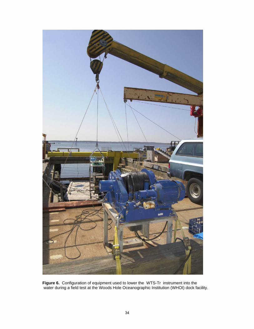
Figure 6. Configuration of equipment used to lower the WTS-Tr instrument into the water during a field test at the Woods Hole Oceanographic Institution (WHOI) dock facility.

34

Figure 7. Collection and volume measurements of water pumped through the WTS-Tr system during testing procedures at the WHOI dock facility.

35

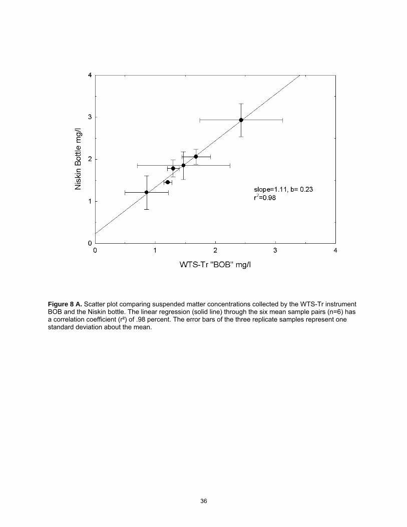
Figure 8 A. Scatter plot comparing suspended matter concentrations collected by the WTS-Tr instrument BOB and the Niskin bottle. The linear regression (solid line) through the six mean sample pairs (n=6) has a correlation coefficient (r²) of .98 percent. The error bars of the three replicate samples represent one standard deviation about the mean.

36

Figure 8 B. Scatter plot comparing suspended matter concentrations collected by the WTS-Tr instrument TED and the Niskin bottle. The linear regression (solid line) through the nine mean sample pairs (n=9) has a correlation coefficient (r²) of .72 percent. The error bars derived from each of the three replicate samples represent one standard deviation about the mean.

37

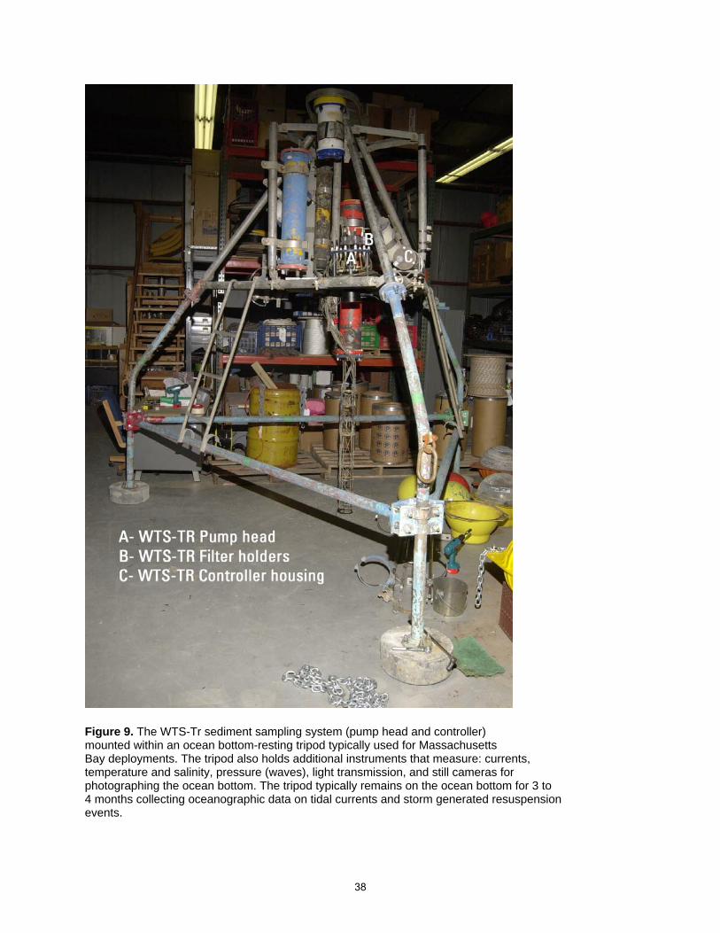
Figure 9. The WTS-Tr sediment sampling system (pump head and controller) mounted within an ocean bottom-resting tripod typically used for Massachusetts Bay deployments. The tripod also holds additional instruments that measure: currents, temperature and salinity, pressure (waves), light transmission, and still cameras for photographing the ocean bottom. The tripod typically remains on the ocean bottom for 3 to 4 months collecting oceanographic data on tidal currents and storm generated resuspension events.

38

Figure 10. The "Y" tube configuration of the McLane WTS-P suspended sediment sampler. This setup allows for flushing of the system with filtered water before and after sampling so as to minimize cross contamination from previously filtered samples.

39

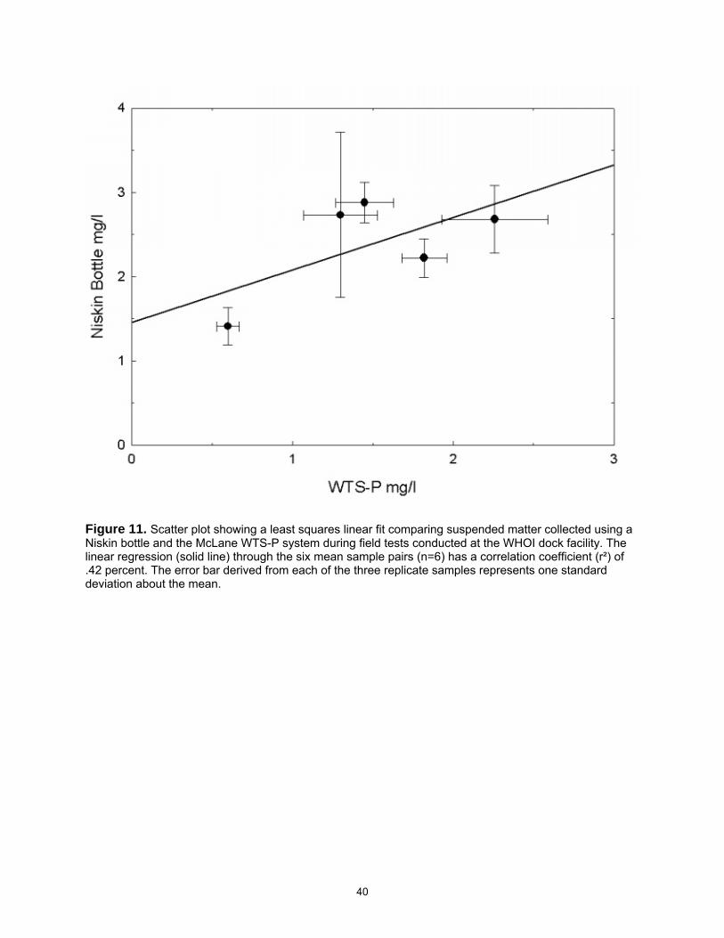
Figure 11. Scatter plot showing a least squares linear fit comparing suspended matter collected using a Niskin bottle and the McLane WTS-P system during field tests conducted at the WHOI dock facility. The linear regression (solid line) through the six mean sample pairs (n=6) has a correlation coefficient (r²) of .42 percent. The error bar derived from each of the three replicate samples represents one standard deviation about the mean.

40

Table 1. Results of suspended matter concentrations (mg/l) collected using filter holders from the WTS-Tr instrument with the internal top frit in place and removed. Results from the standard laboratory millipore filtration system were used as a control. The coefficient of variation is the standard deviation expressed as a percentage of the mean.

Frit Configuration Weight of Volume mg/L Mean Standard Coefficent

suspended matter (mg)

filtered (ml) deviation of variation (%)

Frit in Place 0.829 493 1.68

0.499 413 1.21 1.37 0.27 19.59

0.640 525 1.22

Frit Removed 1.11 493 2.26 1.22 495 2.46 2.44 0.17 7.00

1.37 525 2.60

Millipore 1.42 535 2.65 Rig 1.45 520 2.79 2.83 0.21 7.36

1.59 520 3.06

41

Table 2. Suspended matter concentrations (mg/l) collected over time at the Woods Hole Oceanographic Institution (WHOI) dock facility by the two WTS-Tr instruments TED and BOB and a Niskin bottle. Sd= standard deviation.

Date sample WTS-

Tr BOB

sd Niskin sample NISKIN sd Date samples WTS-Tr TED sd Niskin

sample NISKIN sd

mg/l mean mg/l mg/l mean

mg/l mg/l mean mg/l mg/l mean mg/l

5/96 1.89 1.68 0.24 2.20 2.06 0.18 6/95 2.56 2.56 0.04 4.03 3.68 0.31

1.73 1.86 2.53 3.50 1.42 2.13 2.60 3.50

1/97 1.18 1.21 0.07 1.46 1.45 0.01 1/96 2.67 2.34 0.49 4.06 3.96 0.61 1.29 1.46 2.57 4.51 1.17 1.44 1.78 3.31

8/97 3.14 2.43 0.69 3.38 2.93 0.39 9/96 1.63 1.58 0.36 2.19 2.16 0.07 2.38 2.74 1.19 2.08 1.77 2.67 1.91 2.20

4/99 0.45 0.86 0.36 0.75 1.21 0.40 5/97 2.73 2.42 0.42 2.05 2.06 0.10 1.15 1.41 2.59 2.16 0.98 1.47 1.95 1.97

2/00 1.19 1.30 0.10 2.00 1.78 0.20 1/99 1.23 1.32 0.11 1.60 1.65 0.08 1.36 1.70 1.45 1.74 1.35 1.64 1.28 1.61

9/00 2.25 1.47 0.77 2.21 1.85 0.33 4/99 0.66 1.29 0.86 no data 1.47 1.78 2.27 0.70 1.56 0.95

5/00 1.40 1.16 0.26 1.21 1.18 0.23 0.89 1.41

1.18 0.94 1/01 1.10 0.95 0.13 1.14 1.07 0.14 0.87 0.91 0.90 1.16 5/02 1.43 1.64 0.30 1.76 2.35 0.62 1.85 3.00 2.30 2/3/2003 1.75 1.41 0.33 1.65 1.71 0.05 1.10 1.75 1.37 1.73

42

Table 3. Suspended matter concentrations (mg/l) collected at the Woods Hole Oceanographic Institution (WHOI) dock facility by the WTS-P instrument. The results of the suspended matter concentrations reflect simulated "storm" induced events (sampling actuated from responses of the pressure transducer by raising and lowering the instrument through the water column). The WTS-P and Niskin bottle samples were collected during the same time frames. Due to a Niskin bottle malfunction, only two Niskin samples were collected on the March 2001 test date. Sd= standard deviation.

Date sample WTS-P sd Niskin sample Niskin sd

mg/l mean mg/l mg/l mean mg/l

8/98 1.23 2.34

1.54 1.30 0.23 2.28 2.73 0.98 1.02 2.12 1.41 4.19

3/01 0.70 1.56

0.61 0.60 0.07 1.25 1.41 0.22 0.65 0.54 0.65 0.50 0.58 0.59

6/02 1.44 3.01

1.37 1.45 0.18 2.77 2.88 0.24 1.22 2.55 1.55 2.89 1.68 3.17

8/02 1.95 2.13

1.91 2.26 0.33 2.22 2.68 0.40 2.08 2.87 2.43 2.87 2.62 2.87 2.62 3.10

8/3/2004 2.00 2.63

1.78 1.82 0.14 2.13 2.22 0.23 1.61 2.14 1.88 2.06 1.81 2.15

43

Table 4. Results of preliminary laboratory tests to determine suspended matter concentrations using the

WTS-P and a siphon tube (used as a control) with different sediment grain sizes and flow rates.

Sample raw wt. (mg)vol. filtered

(ml) mg/l MeanStandard Deviation

WTS-P/Siphon tube %

Sediment Trap Sample S60-13

WTS-P, a 10 mg/l solution 0.93 101.38 9.17@ 100 ml/min flow rate with 1.02 103.47 9.86 9.43 0.37

0.88 97.19 9.2799.9%

Siphon tube at same 0.75 80.24 9.35 parameters as above 0.65 67.01 9.70 9.44 0.23

0.88 94.89 9.27

WTS-P, a 10 mg/l solution 1.15 131.80 8.73@ about 50 ml/min flow rate 1.05 115.23 9.11 8.69 0.44

0.86 104.39 8.2499.5%

Siphon tube at same 1.04 109.44 9.50parameters as above 0.90 103.62 8.69 8.73 0.74

0.74 92.25 8.02

Muddy bottom sediment from the continental shelf

WTS-P ~4 MG/L 1.63 497.98 3.40@ 125 ML/MIN FLOW RATE 1.74 508.50 3.43 3.40 0.04

1.68 499.78 3.3688.1%

SIPHON TUBE ~4 MG/L 1.66 486.40 3.42@ 125 ML/MIN 2.11 503.00 4.20 3.86 0.40

1.83 460.50 3.97

WTS-P ~4 MG/L 1.24 447.98 2.76 2.8 0.06@ 50 ML/MIN 1.45 511.48 2.84

71.4%

SIPHON TUBE ~4 MG/L 1.83 450.60 4.06 3.92 0.20@ 50 ML/MIN 1.76 465.90 3.78

Sand (0.125-0.0625 mm) FROM QUISSETT HARBOR

WTS-P ~15 MG/L @ 125 1.13 515.58 2.19 3.22 0.45ML/MIN FLOW RATE 2.08 488.98 4.25 28.5%

SIPHON TUBE ~15 MG/L @ 4.79 494.30 9.68 11.31 2.31125 ML/MIN FLOW RATE 6.10 471.70 12.94

95.2%*sampled using a beaker 4.80 497.30 9.65 11.88 3.15from middle of bucket 7.46 514.20 14.51

*Siphon/beaker as %. This confirms the results of the siphon.

44

Appendix 1. McLane Research Laboratories, USA Water Transfer System ? 18 Program PUMP V1.42 ************************** * MAIN MENU * ************************** S/N 521 ?? transmissometer version <1> Set clock <2> Display time, temperature & voltage <3> Run pump motor <4> Move valve <5> Preload filters <6> Create schedule <7> Run schedule and deploy <8> Offload data to a disk <9> Display data from a disk Exit program Call MAIN MENU Computer Font User Font Select a number 7 Initial pump flow rate (mL/minute) ? ? ? ? ? ? ? ? ? (50?125) 100 Total flow (mL) ? ? ? ? ? ? ? ? ? (10?100000) 3000 Minimum pump flow rate (mL/minute) ? ? ? ? ? ? ? ? ? (20?100) 50 Maximum pumping time (minutes) ? ? ? ? ? ? ? ? ? (1?7200) 120 Begin reading transmissometer data YEAR ? ? ? ? ? ? (0?99) 1 Begin reading transmissometer data MONTH ? ? ? ? ? (1?12) 10 Begin reading transmissometer data DAY ? ? ? ? ? ? (1?31) 24 Begin reading transmissometer data HOUR ? ? ? ? ? ? (0?23) 8 Stop reading transmissometer data YEAR ? ? ? ? ? ? (0?99) 2 Stop reading transmissometer data MONTH ? ? ? ? ? (1?12) 2 Stop reading transmissometer data DAY ? ? ? ? ? ? (1?31) 4 Stop reading transmissometer data HOUR ? ? ? ? ? ? (0?23) 8 Use transmissometer to trigger pump (1=yes 0=no) ? ? (0?1) 1 Minimum transmissometer trigger threshold (mV) ? ? ? (0?5000) 3500 Number of summed transmissometer intervals ? ? ? ? ? (2?960) 128 First to middle storm event maximum time (hrs) ? ? (1?1000) 72 Middle to final storm event maximum time (hrs) ? ? (1?1000) 136 Max number of storms to sample ? ? ? ? ? ? ? ? ? ? ? (0?6) 4 Computer Font User Font 50% deployment no storm threshold reduction (%) ? ? ? (0?100) 10 75% deployment no storm threshold reduction (%) ? ? ? (0?100) 5 85% deployment no storm threshold reduction (%) ? ? ? (0?100) 3 Time between ON and OFF dates = 103 day(s) 0 hour(s) A/D data will be stored every 1540 seconds [ 25 min(s) 40 sec(s) ] Please standby ? sending information to instrument .... ...................................Verified OK

45

APPENDIX 2 During preliminary tests to measure suspended sediment concentrations with the WTS-Tr, we suspected that the internal top frit supplied with the filter holder by the manufacturer (Figure 5) was removing (pre-filtering) some fraction of the natural assemblage of the suspended matter sample that was being suction filtered onto the Nucleopore filter. This was evaluated in the laboratory by vacuum filtering aliquots from freshly collected seawater through in-line filter holders with and without the internal top frit. The samples were filtered at approximately the same vacuum as pressure created by the WTS-Tr instrument (10-15 inches of mercury). Test results showed that the average mean concentration of suspended matter collected with a top frit in place was 44% lower than the mean value with the frit removed (Table 1). This indicates significant trapping of material by the top frit. The frit has large openings (1mm x 2mm) but can trap filamentous organic matter on its gridwork. Based on these test results, the top frits have been removed from all filter holders during laboratory and field-testing and actual long-term field deployments In addition, these results were compared to replicate samples filtered through a standard glass Millipore chimney type filter holder that has no tubing or other potential constriction to the flow. The suspended matter concentrations determined with the in-line filter holder without top frit were an average of 14% lower than measured using the Millipore holder. A probable explanation for the lower values is that some adsorption of particles by the tubing and filter housing takes place. Samples of surface coastal waters containing filamentous or gelatinous particles of biological origin are expected to experience greater losses flowing through tubing and connectors than resuspended bottom sediment that is likely to have a greater fraction of lithogenic particles

46

Appendix 3 Results comparing the suspended matter concentrations collected with the WTS-Tr instruments (designated BOB and TED) with those of the Niskin bottle are shown in Table 2. Scatter plots were constructed showing the linear relationship between the two sets of mean values for all test dates. A high positive correlation (r²= 0.98) exists between the mean suspended matter concentrations (n=6 data pairs) collected by the WTS-Tr BOB system and the Niskin bottle (Figure 8A). There is considerable variability of suspended matter concentrations as shown by the standard deviations plotted as error bars (Figure 8A). Suspended matter concentrations determined with the WTS-Tr BOB were, on average, 21 % lower than those determined by the Niskin bottle. Data and plots comparing WTS-Tr TED with the Niskin bottle were similar. The linear correlation coefficient (r²= 0.72) was high between the mean suspended matter concentrations (n=9 data pairs) collected by the WTS-Tr TED and Niskin bottle system (Figure 8B) and, on average, the concentrations determined with WTS-Tr TED were 23% lower than those determined using the Niskin bottle. There are a number of possible reasons why the WTS systems give lower results than the Niskin bottle system and why both systems have considerable variability. We suspect that the lower suspended matter concentrations determined using the WTS systems indicates that the tubing, connectors, and filter holder upstream of the filter remove some particulates. In contrast, the Niskin bottle has no tubing and the Millipore vacuum filter apparatus has no connectors above the filter and smooth glass surfaces that are easily rinsed. Based on microscopic analysis, the suspended particulates collected from these tidally mixed surface water contained filamentous organic matter, living plankton, and sometimes gelatinous masses, which may have been partially trapped along the flow path of the WTS system. The variability of results obtained in dock tests could be due to the dynamic conditions at the site. During some of the tests, tidal currents were in the range of 50-100 cm/sec and considerable turbulence was observed around support pilings. Variable concentration and composition of suspend sediment would not be unusual over short time scales under these conditions although a continuously recording optical sensor was not used to confirm this assumption. The WTS and Niskin systems may have sampled different turbulent eddies within the flowing water. Although both are triggered at the same depth and at the same time, the WTS pumps for about 5 minutes with individual samples separated by at least 10 minutes. The Niskin bottle encloses its sample of water in a fraction of a second. Hence, the samples collected by the two systems are measuring variability in the flowing water mass on different time Another possible cause of the difference between systems and the variability in results of the WTS is the behavior of flow entering a downward looking intake port and whether the intake port is upstream or downstream of other structures

47

on the instrument. Flow into the intake is not isokinetic, meaning that flow does not enter the port at the same speed and direction as the ambient current (Webb and Radtke, 2003). A somewhat related issue is that the intake port could have been on the upstream side of the instrument and in less local turbulence during some pumping events and down stream of the instrument in greater local turbulence during others. The impact of the non-isokinetic nature of the intake port, and its behavior in different local turbulence, could not be evaluated. A port that always points into the current, as described by Sternberg et al. (1986), may be an advantage that should be explored in future tests.

As mentioned elsewhere in this report, the dock offers the advantages of depth (greater overpressure) and convenient capability for deploying and recovering the samplers. The disadvantage of this test site is the variability in oceanographic conditions. Future tests should be conducted in a test tank that is 30 feet deep and has the capability for complete mixing of suspended matter of selected composition and concentration.

48

Appendix 4 McLane Research Laboratories, USA Water Transfer System Version: atwts1_3.c ÕÍÍÍÍÍÍÍÍÍÍÍÍÍÍÍÍÍÍÍÍÍÍÍÍÍÍÍÍÍÍÍÍÍÍÍÍÍÍ͸ ³ Main Menu ³ ÔÍÍÍÍÍÍÍÍÍÍÍÍÍÍÍÍÍÍÍÍÍÍÍÍÍÍÍÍÍÍÍÍÍÍÍÍÍÍÍ3/4 S/N 453 PORT == 0 Thu Jan 3 15:30:12 2002 <1> Set Time <5> Deploy System <2> Diagnostics <6> Offload Data <3> Fill containers <7> Adjust 'ducer constants <4> Sleep <8> About <9> EEPROM data backup cache Computer Font User Font Selection ? 5 The previous data set will be erased - continue (Yes/No) [Y] Clock reads 01/03/102 15:30:18 Change time & date (Yes/No) [N] ? Enter date & time of deployment [01/03/102 15:30:21] ? 1/3/10215:45:00 Enter time delay until calibration sample [hr] (0 to 24) ? 0 Enter expected recovery date [01/03/102 15:30:45] ? 1/5/102 8:00:00 Enter expected number of storms (1 to 22) ? 1 Enter number of samples per storm (1 to 22) ? 1 > schedule ..... ------------------VERIFICATION------------------- Event 1 of 22 = 01/03/102 15:45:00 Event 2 of 22 = 01/03/102 17:21:36 Event 3 of 22 = 01/03/102 19:12:00 Event 4 of 22 = 01/03/102 21:02:24 Event 5 of 22 = 01/03/102 22:52:48 Event 6 of 22 = 01/04/102 00:43:12 Event 7 of 22 = 01/04/102 02:33:36 Event 8 of 22 = 01/04/102 04:24:00 Event 9 of 22 = 01/04/102 06:14:24 Event 10 of 22 = 01/04/102 08:04:48 Event 11 of 22 = 01/04/102 09:55:12 Event 12 of 22 = 01/04/102 11:45:36 Event 13 of 22 = 01/04/102 13:36:00 Event 14 of 22 = 01/04/102 15:26:24 Event 15 of 22 = 01/04/102 17:16:48 Event 16 of 22 = 01/04/102 19:07:12-> press any key Event 17 of 22 = 01/04/102 20:57:36 Event 18 of 22 = 01/04/102 22:48:00 Event 19 of 22 = 01/05/102 00:38:24 Event 20 of 22 = 01/05/102 02:28:48 Event 21 of 22 = 01/05/102 04:19:12 Event 22 of 22 = 01/05/102 06:09:36 Computer Font User Font

Modify an event (Yes/No) [N] ? Enter PSDEV threshold that indicates a storm wave event [mbar](>0.01) 25

Enter PSDEV threshold duration [minutes] (1 to 1440) ? 240 49

Enter delay between storms [hrs] (0 to 240) ? 240 Enter number of pressure readings per PSDEV calculation (30 to 100) ? 50 Enter interval between PSDEV calculations [min] (1 to 240) ? 10 Enter interval A1 [minutes] (10 to 600) ? 300 Enter interval A2 [minutes] (10 to 600) ? 300 Enter sampling interval between maxima [minutes] (1 to 5760) ? 360 Enter time delay between maxima [minutes] (0 to 359) ? 240 Enter %% of elapsed deployment for first reduction (0 to 100) ? 0 Enter %% of elapsed deployment for second reduction (1 to 100) ? 1 Enter %% of elapsed deployment before time-series only (2 to 100) ? 2 Enter %% of threshold reduction (1st reduction) (0 to 100) ? 0 Enter %% of threshold reduction (2nd reduction) (0 to 100) ? 0 DATE PSDEV threshold 01/03/102 15:33:02 25.00 <-- start 01/03/102 15:45:00 25.00 01/03/102 16:09:09 25.00 01/03/102 16:33:18 0.00 <-- Intervals only. Enter pumping flow rate [ml/min] (50 to 125) ? 100 Computer Font User Font Enter minimum flow rate [ml/min] (20 to 100) ? 50 Enter volume per sample [ml] (10 to 10000) ? 150 Enter pumping time limit [seconds] (1 to 190) ? 150 Enter flushing water volume [ml] (0 to 500) ? 50 Enter the sampling period for pumping flow rates [secs] (1 to 60) ? 30 Current Header reads - lab test of scheduled events only Do you want a different header (Yes/No) [N] ? System shows the following - 01/03/102 15:33:28 28.5 Vb 17 øC 1008 mb 14.6 psi PORT = 00 Are you ready to deploy (Yes/No) [N] ? y System is ready. Remove communication cable & deploy ----------------------<< MONITOR MODE >>------------------------------- <01/03/102 15:33:34> Waiting:Event #1:calibration sample @ 01/03/102 15:45:00 <01/03/102 15:33:35> Sleeping . . .

50

Appendix 5 McLane Research Laboratories, USA

Water Transfer System Version: atwts1_3.c ╒═══════════════════════════════════════╕ │ Main Menu │ ╘═══════════════════════════════════════╛ S/N 453 PORT == 0

Fri Jan 18 10:28:04 2002 <1> Set Time <5> Deploy System <2> Diagnostics <6> Offload Data <3> Fill containers <7> Adjust 'ducer constants <4> Sleep <8> About <9> EEPROM data backup cache User Font Computer Font Selection ? 5 Clock reads 01/18/102 10:28:07 Change time & date (Yes/No) [N] ? Enter date & time of deployment [01/18/102 10:28:10] ? 1/18/102 10:35:00 Enter time delay until calibration sample [hr] (0 to 24) ? 0 Enter expected recovery date [01/18/102 10:28:31] ? 1/30/102 8:00 Enter expected number of storms (1 to 22) ? 4 Enter number of samples per storm (1 to 5) ? 5 > schedule ..... ------------------VERIFICATION------------------- Event 1 of 3 = 01/18/102 10:35:00 Event 2 of 3 = 01/22/102 09:39:31 Event 3 of 3 = 01/26/102 08:49:45 Modify an event (Yes/No) [N] ? Enter PSDEV threshold that indicates a storm wave event [mbar](>0.01) ? 35 Enter PSDEV threshold duration [minutes] (1 to 1440) ? 2 Enter delay between storms [hrs] (0 to 240) ? 0 Enter number of pressure readings per PSDEV calculation (30 to 100) ? 60 Enter interval between PSDEV calculations [min] (2 to 2) ? 2 Enter interval A1 [minutes] (2 to 600) ? 4

51

Computer Font User Font Enter interval A2 [minutes] (2 to 600) ? 4 Enter sampling interval between maxima [minutes] (1 to 5760) ? 4 Enter time delay between maxima [minutes] (0 to 3) ? 3 Enter %% of elapsed deployment for first reduction (0 to 100) ? 50 Enter %% of elapsed deployment for second reduction (51 to 100) ? 70 Enter %% of elapsed deployment before time-series only (71 to 100) ? 80 Enter %% of threshold reduction (1st reduction) (0 to 100) ? 20 Enter %% of threshold reduction (2nd reduction) (20 to 100) ? 30 DATE PSDEV threshold 01/18/102 10:30:18 35.00 <-- start 01/24/102 09:17:30 28.00 01/26/102 18:22:30 24.50 01/27/102 22:55:00 0.00 <-- Intervals only. Enter pumping flow rate [ml/min] (50 to 125) ? 100 Enter minimum flow rate [ml/min] (20 to 100) ? 50 Enter volume per sample [ml] (10 to 10000) ? 250 Enter pumping time limit [seconds] (1 to 310) ? 300 Enter flushing water volume [ml] (0 to 500) ? 20 Enter the sampling period for pumping flow rates [secs] (1 to 60) ? 30 Current Header reads - Do you want a different header (Yes/No) [N] ? System shows the following - 01/18/102 10:30:45 27.4 Vb 6 EC 2349 mb 34.1 psi PORT = 00 Are you ready to deploy (Yes/No) [N] ? y System is ready. Remove communication cable & deploy

52

Appendix 6

Preliminary comparisons of the WTS-P and other sampling/filtration methods: Two approaches were used to evaluate the sampling efficiency of the WTS-P unit. The first involved tests at the WHOI dock at a depth of 30 feet where the WTS-P system was compared to a conventional Niskin bottle and Millipore vacuum system as discussed earlier. The second approach, conducted in the laboratory, evaluated the performance of the WTS-P in response to changes in particle sizes and flow rates through the sampler.

Results of the tests at the dock showed that suspended matter concentrations determined with the WTS-P system were 62% on average of those measured with the Niskin bottle (Table 3). There was a considerable amount of variability in suspended matter concentrations in samples collected a few minutes apart and only a fair correlation when results of one method were plotted against the other (Figure 11, r² = 0.42). As discussed in a previous section, there are several possible reasons for the discrepancy and the variability. High tidal current velocities at the dock may result in non-uniform suspended matter concentrations over short time scales. The natural assemblage of particulate surface water at the dock is likely to include filamentous organic particles (i.e. living plankton) that may be preferentially trapped in the small orifices and tubing of the WTS-P instrument before reaching the filter. The intake port fixed to the WTS-P instrument package was not consistently oriented with respect to current direction. A difference in efficiency of drawing particles into a tube from the upstream side or from the more turbulent downstream side of the instrument is suspected but has not been evaluated.

The second series of tests were preformed in the laboratory where the suspended matter composition and concentration could be controlled. The laboratory tests were conducted using material collected from a near-bottom sediment trap in Massachusetts Bay. This material was sieved through a 1000-micron screen to remove juvenile clams that had set on the trap surfaces. The sieved material consisted of 10% sand (made up largely of thin carbonate fragments), 40% silt, and 50% clay. The fine grained, high carbonate and organic-rich sediment probably more closely simulates the suspended sediment encountered by the WTS-P during a deployment in Massachusetts Bay than the material suspended in near surface water at the dock.

A suspension of trap material was prepared in a 16-liter supply bucket and kept well mixed by a mechanical stirrer. Two siphon tubes were fixed in the center of the supply bucket. One tube directed suspension through the manifold, tubing and connectors of the WTS-P (without a filter) to a collection beaker. The other tube emptied directly to a beaker. The test was designed to evaluate the potential losses of particles as the suspension flowed through the plumbing of the WTS-P. The flow rates were 100 ml/min and about 50 ml/min, controlled by adjusting the hydraulic head between supply bucket and collection beaker. The higher rate is

53

close to the starting pumping speed of 125 ml/min, and the lower rate is the limit at which pumping is turned off. Suspended matter concentrations on all samples were determined by filtering a known volume of sample through a pre-weighed Nuclepore filter (0.4 micron pore diameter) in a Millipore vacuum filtration system.

The concentrations of suspended sediment trap material collected through the WTS-P and through the straight tube were essentially identical at both the high and the low flow rate (Table 4). These results indicated that the sediment trap material was not removed by the internal plumbing of the WTS-P.

Other tests were conducted using a suspension of surficial bottom sediment from the continental shelf consisting of 7% very fine sand (made up largely of lithogenic particles), 67% silt, and 26% clay. The suspended matter concentrations determined on the suspension flowing through the WTS-P were on average 88% of the value flowing through the siphon tube at a flow rate of 125 ml/min and 71% at a flow rate at 50 ml/ min. Additional tests used a suspension of very fine sand (6.25-125 micron) sieved from a local beach. The concentration of sand suspension flowing through the WTS-P was 29% of the concentration passing through the siphon tube at a flow rate of 125 ml/min. It is worth noting that the very fine sand (62.5-125 micron) is not representative of natural sediment. It was used to test the flow-through of the coarser grain sizes.)

These observations indicate a significant under sampling of lithogenic particles as the particle grain size increases. The cause for this under sampling this sediment type is not obvious. The minimum speed of the suspension passing through the WTS-P is greater than 9 cm/sec (at 50-ml/min-flow rate) which is 10 times higher than the settling velocity of a quartz grain having diameter 0.125 mm (fine sand). An accumulation of coarse grains has never been apparent at the junction of connectors. To evaluate this issue further, additional testing is required using higher pumping rates and filters with higher permeability. Ideally, these tests should be performed in a tank in which overpressures equivalent to 30 feet water depth (about 1 atmosphere). This overpressure prevents the cavitation when the pump draws a negative pressure as filters become clogged. The other important feature of any test tank is the capability for maintaining a well-mixed suspension of known composition and concentration.

54

Appendix 7. McLane Research Laboratories, USA Water Transfer System Version: atwts1_3.c +---------------------------------------+ ¦ Main Menu ¦ +---------------------------------------+ S/N 453 PORT == 99 Wed Feb 6 08:15:11 2002 <1> Set Time <5> Deploy System <2> Diagnostics <6> Offload Data <3> Fill containers <7> Adjust 'ducer constants <4> Sleep <8> About <9> EEPROM data backup cache Computer Font User Font Selection ? 5 Searching for home port ... Home found Clock reads 02/06/102 08:16:58 Change time & date (Yes/No) [N] ? Enter date & time of deployment [02/06/102 08:17:42] ? 2/7/102 8:00:00 Enter time delay until calibration sample [hr] (0 to 24) ? 24 Enter expected recovery date [02/06/102 08:18:17] ? 5/20/102 8:00:00 Enter expected number of storms (1 to 22) ? 4 Enter number of samples per storm (1 to 5) ? 5 > schedule ..... --------------------------VERIFICATION------------------------------- Event 1 of 3 = 02/08/102 08:00:00 Event 2 of 3 = 03/12/102 16:13:04 Event 3 of 3 = 04/16/102 00:06:31 Modify an event (Yes/No) [N] ? Enter PSDEV threshold that indicates a storm wave event [mbar](>0.01) ? 25 Enter PSDEV threshold duration [minutes] (1 to 1440) ? 240 Enter delay between storms [hrs] (0 to 240) ? 24 Enter number of pressure readings per PSDEV calculation (30 to 100) ? 50 Computer Font User Font Enter interval between PSDEV calculations [min] (1 to 240) ? 10 Enter interval A1 [minutes] (10 to 600) ? 300 Enter interval A2 [minutes] (10 to 600) ? 300 Enter sampling interval between maxima [minutes] (1 to 5760) ? 360 Enter time delay between maxima [minutes] (0 to 359) ? 240 Enter %% of elapsed deployment for first reduction (0 to 100) ? 50 Enter %% of elapsed deployment for second reduction (51 to 100) ? 70 Enter %% of elapsed deployment before time?series only (71 to 100) ? 80 Enter %% of threshold reduction (1st reduction) (0 to 100) ? 20 Enter %% of threshold reduction (2nd reduction) (20 to 100) ? 30 Current Header reads - Do you want a different header (Yes/No) [N] ? System shows the following -

55

02/06/102 08:22:17 31.5 Vb -2EC 1031 mb 15.0 psi PORT = 00 Are you ready to deploy (Yes/No) [N] ? y System is ready. Remove communication cable & deploy

56