an invitation to cognitive science - 2nd edition: vol. 4 ...wexler.free.fr/library/files/swets...

This excerpt from

An Invitation to Cognitive Science - 2nd Edition: Vol. 4.Don Scarborough and Saul Sternberg, editors.© 1998 The MIT Press.

is provided in screen-viewable form for personal use only by membersof MIT CogNet.

Unauthorized use or dissemination of this information is expresslyforbidden.

If you have any questions about this material, please [email protected].

Chapter 13

Separating Discrimination and Decision in

Detection , Recognition , and Matters of Life and

Death

John A . Swets

Editors'

Introduction

This chapter explains signal detection theory (SOT) and illustrates the remarkable variety of

problems to which it can be applied. When it was first developed (by the author of this

chapter, among others), SOT revolutionized the way we think about the perfonnance of sensory tasks, by explaining how perfonnance depends not only on sensory infonnation, but

also on decision process es. The theory also provided ways to disentangle these two aspectsof perfonnance- to decompose .or separate the underlying operations into sensory anddecision process es and to decide whether the decision process is optimal, given the sensoryinfonnation. Now, after four decades of research, we are led to the surprising conclusion that

many tasks we perfonn, in domains ranging &om memory recall to airplane maintenance, are

analogous to sensory detection, and can be analyzed within the &amework of this theory.SOT asserts that perfonnance in a discrimination or detection task must be divided into at

least two stages. In the first stage, infonnation about some situation is collected; in the second

stage, this "signal" is evaluated for decision making. The signal provided by the first

stage is often "noisy," which is to say, mixed with irrelevant material, and the second stage

must evaluate the noisy signal provided by the first stage. To take a simple example, if anobserver tries to decide whether she hears a faint sound, the message reaching her brain maybe contaminated by noise, such as the variable sounds of her own pulse and breathing. One

consequence of the noise is that decisions will sometimes be wrong. But the observer hassome control over the errors that she makes. To use John Swets's terminology, there are two

types of errors: false positives (e.g., asserting you heard something when there was nothingthere) and false negatives (e.g., asserting you did not hear anything when there really was asound). SOT explains how an observer can reduce the chance of one type of error, but onlyat the cost of increasing the chance of the other. (Can you see how a jury verdict might be afalse positive or a false negative error, and how trying to reduce one type of error will affectthe chance of the other?) SOT also predicts how observers will choose to balance the two

types of errors.SOT has its origins in work on noisy communication systems. Oevices such as radars,

radios, and TVs are all susceptible to electrical interference (one type of noise) and the engineering problem was how to determine when there was a "signal

" (e.g., a radar image of a

missile) within the obscuring noise. The big insight for psychology was that all communications

systems, whether they be sensory systems, messages within the brain, or messagesbetween people, have to deal with noise, particularly when the signal is weak. Early studieson perception showed that in audition and vision, the message that reached the brainwas indeed noisy. Later studies showed that the retrieval of a weak memory could also be

desaibed as an attempt to find the signal (memory) in the noise. SHII other studies haveshown that a radiologist examining an Xray for evidence of cancer or an airplane technicianexamining a plane for evidence of stress cracks faces a similar situa Hon, as Swets describes inthis chapter. Other research shows that SDT can be applied to other important social questions

, such as the reliability of blood tests for AIDS. Unfortunately, too few people yetappreciate the importance and broad applicability of SDT.

The work that Swets has done on many prac Hcal problems exemplifies the deep contributions that psychology can make. Swets discuss es how a doctor examines an Xray for

evidence of cancer. If you have ever seen an Xray , you know that it presents a vagueshadowy image. The doctor's task is to make a decision on the basis of this vague image.This example illustrates a property of many decision-making situations. There may be severaltell-tale signs of cancer in the Xray , and the doctor must combine this information. Becausethis is often difficult to do reliably, Swets and his colleagues have developed computer programs

to help doctors in this situation. This applica Hon makes use jointly of the strengths ofhumans and machines, and is therefore especially interesting in the context of cognitivescience. And SDT can make important contributions to many other practical decision-makingsituations. It does not surprise us that in the 1994 White House policy report Science in theNational Interest, Swets's work on signal detection theory and its applicability in an array ofhigh-stakes decision-making set Hngs was selected to illustrate the importance of basicbehavioral science research.

Although there is a difference in terminology between Swets's discussion of the decisionproblem in detection and Wickens's discussion of the testing of statistical hypotheses (chap.12, this volume), you will discover strong similarities.

636 Swets

638

Chapter Contents

13.1 Introduction 63713.1.1 Detection, Recognition, and Diagnostic Tasks 63713.1.2 The Tasks' Two Component Process es: Discrimination and Decision13.1.3 Diagnosing Breast Cancer by Mammography: A Case Study 639

13.1.3.1 Reading a Mammogram 63913.1.3.2 Decomposing Discrimination and Decision Process es 642

13.1.4 Scope of This Chapter 64313.2 Theory for Separating the Two Process es 644

13.2.1 Two-by- Two Table 64413.2.1.1 Change in Discrimination Acuity 64713.2.1.2 Change in the Decision Criterion 64813.2.1.3 Separation of Two Process es 649

13.2.2 Statistical Decision and Signal Detection Theories 64913.2.2.1 Assumptions about the Observation 65013.2.2.2 Distributions of Observations 65113.2.2.3 The Need for a Decision Criterion 65313.2.2.4 Decision Criterion Measured by the Likelihood Ratio 65413.2.2.5 Optimal Decision Criterion 65413.2.2.6 A Traditional Measure of Acuity 656

1.3.3 The Relative Operating Characteristic 65713.3.1 Obtaining an Empirical ROC 65813.3.2 A Measure of the Decision Criterion 65913.3.3 A Measure of Discrimination Acuity 65913.3.4 Empirical Estimates of the Two Measures 661

Separating Discrimination and Decision 637

13.4 Illustrations of Decomposition of Discrimina Hon and Decision 66213.4.1 Signal Detection during a Vigil 66313.4.2 Recognition Memory 66413.4.3 Polygraph Lie Detection 66413.4.4 Information Retrieval 66513.4.5 Weather Forecasting 666

13.5 Computational Example of Decomposition: A Dice Game 66713.5.1 Distributions of Observations 667

Problems 697References 698About the Author 702

13 .1 Introduction

13.1.1 Detection , Recognition , and Diagnostic Tasks

Detection and recognition are fundamental tasks that underlie most complex behaviors . As defined here, they serve to distinguish between two

alternative , confusable stimulus categories . The task of detection is todetermine whether a specified stimulus (of category A , say) is present ornot . For example, is a specified weak light (or specified weak sound, pressure

, aroma, etc.) present or not? If not , we can say that a "null stimulus "

(of category B) is present. The task of recognition is to determine whether

13.5.2 The Optimal Decision Criterion for the Syrnrnetrical Game 66913.5.3 The Optimal Decision Criterion in General 67013.5.4 The likelihood Ratio 67113.5.5 The Dice Game's ROC 67213.5.6 The Game's Generality 673

13.6 Improving Discrimination Acuity by Combining Observations 67413.7 Enhancing the Interpretation of Mammograms 676

13.7.1 Improving Discrimination Acuity 67713.7.1.1 Determining Candidate Perceptual Features 67813.7.1.2 Reducing the Set of Features and Designing the Reading Aid 68013.7.1.3 Determining the Final list of Features and Their Weights 68213.7.1.4 The Merging Aid 68213.7.1.5 Experimental Test of the Effectiveness of the Aids 68413.7.1.6 Clinical Significance of the Observed Enhancement 685

13.7.2 Optimizing the Decision Criterion 68613.7.2.1 The Expected Value Optimum 68613.7.2.2 The Optimal Criterion Defined by a Particular False Positive Proportion

68713.7.2.3 Societal Factors in Setting a Criterion 687

13.7.3 Adapting the Enhancements to Medical Practice 68813.8 Detecting Cracks in Airplane Wings: A Second Practical Example 689

13.8.1 Discrimination Acuity and Decision Criterion 68913.8.2 Positive Predictive Value 69013.8.3 Data on the State of the Art in Materials Testing 69113.8.4 Diffusion of the Concept of Decomposing Diagnostic Tasks 693

13.9 Some History 694

Suggestions for Further Reading 697

a stimulus known to be present is of category A or category B. For example, is this item familiar or new? The responses given in these tasks correspond

directly to the stimulus categories : the observer says "A " or 1' 8."

The task of diagnosis can be either detection or recognition , or both .In the cases of detection and recognition , the focus of this chapter will beon tasks devised for the psychology laboratory , as in the study of perception

, memory , and cognition . In the case of diagnosis , the focus herewill be on practical tasks, such as predicting severe weather , finding cracksin airplane wings , and determining guilt in criminal investigations . As a

specific example of diagnosis , is there something abnormal on this Xrayimage, and, if so, does it represent a malignant or a benign condition ?

Diagnoses are often made with high stakes and, indeed, are often mattersof life and death.

In the tasks of primary interest , an organism , usually a human, makes observations

repeatedly or routinely and each time makes a two -alternativechoice based on that observation . Though considered explicitly here onlyin passing, the ideas of this chapter apply as well to observations (ormeasurements) and choices made by machines.

13.1.2 The Tasks' Two Component Process es: Discrimination andDecision

Present understanding of these tasks acknowledges that they involve two

independent cognitive process es- one of discrimination and one of decision. In brief , a discrimination process assess es the degree to which the

evidence in the observation (for example, perceptual , memorial , or cognitive evidence) favors the existence of a stimulus of category A relative to

B. A decision process, on the other hand, determines how strong the evidence must be in favor of alternative A (or B) in order to make response

A (or B), and chooses A (or B) after each observation depending onwhether or not the requisite strength of evidence is met . We may think ofthe strength of evidence as lying along a continuum from weak to strongand the organism as setting a cutoff along the continuum - a "decisioncriterion ,

" such that an amount of evidence above the criterion leads to a

response of A and an amount below , to a response of B.The observed behaviors in such tasks need to be separated or II decomposed

," so that the discrimination and decision process es can be evaluated

separately and independently . We want to measure the acuity of discrimination- how well the observer assess es the evidence - without regard

to the appropriateness of the placement of the decision criterion ; and wewant to measure the location of the decision criterion - whether strict ,moderate , or lenient , say- without regard to the acuity of discrimination .One reason to decompose is that an observed change in behavior may

638 Swets

reflect a change in the discrimination or the decision process. Anotherreason is that certain variables in the environment or in the person willhave an influence on observed behavior through their effect on the discrimination

process while other variables will be mediated by the decision

process. Often we want to measure what is regarded as a basic process ofdiscrimination , as an inherent capacity of the individual , in a way that isunaffected by decision process es that may vary from one individual toanother and within an individual from one time to another . But as weshall also see, there are instances in which the decision process is the center

of attention .

13.1.3 Diagnosing Breast Cancer by Mammography: A Case Study

The detection, recognition, and diagnostic tasks, and the decompositionof their performance data into discrimination and decision process es,are illustrated here by the diagnostic task that faces the radiologist in

interpreting X-ray mammograms. Radio logical interpretations assess the

strength of the evidence indicative of breast cancer and provide a basis fordeciding whether to recommend some further action. For our purposes,we shall consider the Xrays as belonging to either stimulus category A,"cancer,

" or stimulus category B, "no cancer"; and the corresponding

response alternative to be a recommendation of surgery to providebreast tissue for pathology confirmation (i.e., a biopsy) or a "no action"

recommendation because the breast is deemed "normal" as far as canceris concerned.

13.1.3.1 Reading a Mammogram

It will help here to be concrete about how mammograms are interpretedvisually (how they are "read")- that is, what perceptual features of the

image are taken as evidence for cancer. And later in the chapter, we shallsee how perceptual studies can improve both the acuity of radiologists in

assessing those features and their ability to combine the assessments intoa decision.

Radiologists look for ten to twenty visible features of a mammogramthat indicate, to varying degrees, the existence of cancer. A perceptualfeature is a well-defined aspect or attribute of a mammogram or of someentity within the mammogram. They fall into three categories: (1) the

presence of a "mass," which may be a tumor; (2) the presence of "calcifications

," or sandlike particles of calcium, which in certain configurations

are indicative of cancer, and (3) "secondary signs,

" which are changes inthe form or profile of the breast that often result indirectly &om a cancer.

Though all masses, calcifications, and secondary signs are abnormal,"malignant

" abnormalities indicate a cancer, while "benign" abnormalities


640 Swets

do not . Thus the diagnostic task in mammography is one of detection(is there an abnormality present?) followed by recognition (is a presentabnormality malignant or benign ?).

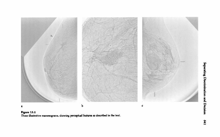
Figure 13.1 illustrates some relevant features. Figure 13.la shows amass, seen as a relatively dark area, located at the intersection of the horizontal

and vertical (crosshair) lines shown at the left and top of the breast.This mass has an irregular shape and an irregular border formed of spikedprojections . These two features, of irregular mass shape and irregular border

, are highly reliable signs of malignancy . The lower part of the breast

image in figure 13.la (above the vertical line at the bottom ) shows somecalcifications . These particular calcifications are probably benign because,compared to malignant ones, they are relatively large and scattered.

The arrow at the top left of figure 13.la points to two kinds of secondary

signs: a slight indentation of the skin and an increased darkness ofthe skin that indicates a thickening of the skin. Both are indicative of a

malignancy .In figure 13.lb , the mass in the center of the image is likely malignant

because it has an indistinct or fuzzy border , indicating (as spiked projections do) a cancerous process spreading beyond the body of the tumor

itself . This mammogram also shows some calcifications - which can occurinside of a mass, as they do here, or outside of a mass. Because these calcifications

are relatively small and clustered, they suggest a malignancy .The mass of figure 13.1c is benign and is, specifically , a relatively harmless

cyst . A cyst has a characteristically round or oval shape and a clearand smooth border .

I hasten to mention that figure 13.1 gives exceptionally clear examplesof malignant and benign abnormalities , to suit a teaching purpose; in

practice, these perceptual features may be very difficult to discern. I wishalso to draw a conceptual point from figure 13.1 that is fundamental todetection , recognition , and diagnostic tasks: observers must often combine

many disparate pieces of information into a single variable , namely ,the degree to which the evidence favors one of the two alternatives in

question , category A relative to category B.We can also think of this degree-of -evidence variable as indicating the

probability that the stimulus is &om category A . Then the observer whomust choose between A and B will set a cutoff , or criterion value, alongan evidence continuum viewed as a probability continuum - in effect,along a scale from 0 to 100. A cutoff at 75, say, means that the probability

that the stimulus is an A must be 0.75 or greater (and that the stimulus is a B, 0.25 or less) for the observer to choose A . As indicated earlier

and developed in more detail later, the evidence may be complex- it may

contain many variables, or many "qimensions

" - but , for purposes of atwo -alternative A or B response, it is best to boil the evidence down to

Separating D

isaimination

and Decision

641

.~x~ a\f~ UJ paql

D Sa PIe

sa~eaJ

l~

da)Jad

SUJMO

\fS 'swe

J8owwew

a A He~snw

aaJ

\U

1 f.lamS

!i

642 Swets

one dimension, namely, the probability of one alternative relative to theother.

13.1.3.2 Decomposing Discrimination and Decision Process es

There is a need to measure the fundamental acuity of the Xray mammo-

gram technique, that is, to measure precisely and validly how well thistechnique is able to separate instances of cancer, on the one hand, frominstances of benign abnormality or no abnormality, on the other. Wedesire a quantitative measure of acuity that is independent of (unaffectedby) the degree to which any or all radiologists are inclined to recommenda biopsy. Several parties wish to know in general terms how accurateXray mammography is so that it can be fairly compared to alternativediagnostic techniques, for example, physical examination (palpation), andthe other available imaging techniques of ultrasound, computerized axialtomography (

"CAT scans" or CT), and magnetic resonance imaging (MRIor MR). Hospital administrators and insurers, as well as physicians andpatients, wish to use a technique that is "cost-effective,

" one that providesthe best balance of high acuity and low cost. They need to appreciate thatthe acuity of diagnostic imaging techniques is fundamentally determinedand set by the limitations of the technology as well as the perceptualabilities of the interpreter, whereas the decision criterion may tend to varysomewhat from one technique to another, and, indeed, can be adjustedby agreement. Moreover, agencies that certify individual radiologists forpractice must know how acute the mammography technique is in eachpractitioner

's hands, irrespective of decision tendencies.Similarly, there is a need to know quantitatively how individual radiolo-

gists set their respective decision criteria, and how the profession generallysets its criterion, for recommending biopsy. A very lenient criterion-

requiring only a little evidence to recommend biopsy (e.g., 5 on a 100-

point scale) might be adopted in order to identify correctly, or "find," a

large proportion of existing cancers. And, in fact, radiologists do set verylenient criteria in reading mammograms, with the idea that early detectionof cancer reduces the risk of fatality. There are constraints, however, onhow lenient the decision criterion can be. A lenient criterion will serve tofind a large proportion of existing cancers, but, at the same time, it willlead to many recommendations of biopsy surgery on noncancerousbreasts and thus increase the number of patients subjected unnecessarilyto such surgery.

Radiologists read mammograms in two different settings, which requiredifferent placements of the decision criterion. In a "screening

" setting,

nonsymptomatic women are given routine mammograms (every year orevery few years), and the proportion of such women actually havingcancer is low, about 2 in 100 (Ries, Miller , and Hankey 1994). In a


"referral" setting, on the other hand, patients have some symptom ofcancer, perhaps a lump felt in the breast. Among such patients, the proportion

having cancer is consider ably higher, about 1 in 3. I suggest laterthat a rather strict criterion is appropriate to the screening situation and arather lenient criterion is appropriate to the referral situation.

It is clear, in any case, that biopsy surgery is expensive financially andemotionally so that unnecessary surgery needs to be curtailed. In fact, alarge number of unnecessary biopsy recommendations can beunmanage-able as well as undesirable. As the government health agencies advise morewomen to undergo routine, annual mammograms, and as more womencomply, the number of pathologists in the country may not be largeenough to accommodate a very lenient biopsy criterion. One way tomeasure the criterion in this case is by the fraction of breast biopsies thatturn out to confirm a cancer: the "yield

" of biopsy. In the United Statesthe yield varies from about 2/ 10 to 3/ 10; approximately 2 or 3 of 10breasts biopsied are found to have cancer (Sickles, Ominsky, and Sollitto1990). England

's physicians generally use a stricter criterion; their biopsyyield is about 5/ 10 (unpublished data from the UK National Breast Screening

Centers, 1988- 1993).

13.1.4 Scope of This Chapter

Although, in using mammography as a case study, I have tried with continual references to make new terms concrete, it will be necessary to treat

the detection, recognition, and diagnostic tasks in formal terms, both to reflect their generality and to show how their performance data can be analyzed into discrimination and decision process es. Section 13.2 shows how

two variables considered in the previous discussion of mammography-the proportion of cancerous breasts recommended for biopsy and the proportion

of noncancerous breasts recommended for biopsy- are the basisfor separating and measuring the two cognitive process es. More generally

, the variables will be considered as the proportion of times that response A is given when stimulus A is present and the proportion of times

that response A is given when stimulus B is present. To show the interplay of these variables in defining measures of acuity and the decision criterion, section 13.2 takes an excursion into a theory of signal detection that

is based on the statistical theory of decision making. Section 13.3 thenshows how both the theoretical ideas and the measures of discrim.inationand decision performance can be represented simply and compactly in asingle graph.

Section 13.4 presents briefly some examples of successful separation ofthe two cognitive process es- examples taken from psychological tasks ofperception and memory and from the practical tasks of polygraph lie

644 Swets

detection, information retrieval, and weather forecasting. With that additional motivation, section 13.5 returns to theory and measurement in

order to reinforce the main concepts via a dice game that you are invitedto playas a calculational exercise.

Section 13.6 briefly describes the theory of how several observationsmay be combined for each decision- much as the radiologist examinesseveral perceptual features of a mammogram- in order to increase discrimination

acuity. Section 13.7 then shows how the radiologists can begiven certain aids to help them attend to the most significant perceptualfeatures, to assess those features better, and to better merge those individual

feature assessments into an estimate of the probability that canceris present; and how these aids improve performance by simultaneously andsubstantially increasing the proportion of cancers found through biopsywhile decreasing the proportion of normal breasts recommended forbiopsy. Ways of setting and monitoring the radiologist

's decision criterion are also discussed.

Section 13.8 treats briefly another practical example, that of humaninspectors using certain imaging techniques to detect cracks in airplanestructures. Data are presented on the state of the art that dramaticallyillustrate the need for separating discrimination and decision process es, inorder to increase acuity and to set appropriate decision criteria- a needthat remains to be appreciated in the materials-testing field.

Finally, section 13.9 gives a historical overview, describing how in the1950s the relevant theory was taken into psychology from statistics,where it applied to testing statistical hypotheses (Wald 1950), via engineering

, where it applied to the detection of radar and sonar signals(Peterson, Birdsall, and Fox 1954), to replace a century-old theory of anessentially fixed decision criterion, equivalent to sensory and memorythresholds (Green and Swets 1966). The diverse diagnostic applications ofthe theory, growing &om the 1960s on, were based originally on psychological

studies showing the validity of the theory for human observers in

simple sensory tasks (Tanner and Swets 1954; Swets, Tanner, and Birdsall1961).

13.2 Theory for Separating the Two Process es

13.2.1 Two-by- Two Table

The statistical theory for separating discrimination and decision process esis based on a two-by-two table, in which data from a task with two stimuli

and two responses appear as counts or frequencies in cells of the table.As shown in table 13.1, the stimulus alternatives (cancer and normal) are

represented at the top of the table in two columns, and the response

Stimulus (

Truth)

Category

A

Category

B

Positive

Negative

- <

~ ~

(I

) (2

)

0 : t : true false

1

~

posi

Hve

positive

U (TP

) (FP

)

~

~ (3

) (4

)

~

. -

0

i

false true

1

Z

negative nega

Hve

U (

FN) ( TN )

alternatives (recommendation of biopsy and of no action ) are representedat the side, in two rows . In general terms, as indicated in the table 13.1,both the stimulus and response alternatives can be called either "

positive"

(cancer exists; a biopsy recommendation is made) or "negative

" (the

patient is normal ; no action is recommended ). The convention is to referto the stimulus of special interest (in our example, cancer) as "positive ,

"

. even when that stimulus produces negative affect. (Colloquially , when the

response is "positive ," the mammogram , or other medical test, is also said

to be "positive").

To acknowledge some terminology that has been implicit in this discussion, and needed beyond psychological studies, the two " stimulus "

categories (A and B) are generally regarded as two alternative "states ofthe world ." They may be conditions or events that follow , instead of precede

, the "response

" made to an observation . For example, the relevantstates of the world follow the "

response" in weather forecasting . And

similarly , the "response

" is more generally called a "decision "; the decision

is a choice between two alternatives that may follow or, instead,

anticipate , the occurrence of one or the other alternative . Establishing thatone or the other of the states of the world actually exists relative to a

particular decision (e.g., confirmation by biopsy ) is said to provide the


Table 13.1The two-by-two table of stimulus (truth) and response (decision). showing the four possibledecision outcomes.

(U

O! S ! : > aa ) as

uods

a

~

"truth" relative to that decision. And so we can ask, 'Which stimulus

occurred?" or 'What is the truth?" For convenience, we shall use mostlythe "stimulus-response

" terms.There are four possible stimulus-response

"outcomes," as shown in

table 13.1. When the positive response coincides with the positive stimulus- for example, when a response to make a biopsy is followed by the

pathologist's confirmatory determination of cancer- the outcome falls in

the cell labeled " I " . It is called a "true positive"

(TP). Cell 2 represents thecoincidence of the negative stimulus and a positive response- for example

, when a biopsy is recommended for a normal patient; this outcome iscalled a "false positive

" (FP). Proceeding, there are "false negative

" (FN)

and "true negative"

(TN) outcomes, as indicated in cells 3 and 4, respec-

tively . In FN no action is recommended even though cancer exists, andin TN no action is recommended and none is necessary. Cells 1 and 4represent correct (true) responses; cells 2 and 3 represent incorrect (false)responses.

The counts or raw frequencies of the four possible co incidences ofstimuli and responses are denoted a, b, c, and d in table 13.2, for cells 1, 2,3, and 4, respectively. As shown, the two column sums are a + c and b + d,and the two row sums are a + b and c + d. The total number of counts isN = a + b + c + d. The proportion of positive stimuli for which a positiveresponse is made is af(a + c) and is denoted here the "true positive proportion"

(TPP). Similarly, we have bf(b + d) or the "false positive pro-

Stimulus ( Truth )

Positive

Negative

~

: c (

1) (

2)

.

~

a b a + b

Q . .

~

: c (3

) (4

)

CG

to

c d c + d

Z

a + c b + d N=

a + b + c + d

(U

O! S ! : > aa ) as

uods

a

' M

646 Swets

Table 13.2-The two-by-two table with cell entries indicating frequencies of stimulus-response outcomes,to provide definitions of the four relevant proportions, as shown.

TPP = a/ (a + c)FPP = b/ (b + d)

FNP = c/ (a + c)TNP = d/ (b + d)

�


portion"

(FPP). The remaining two possibilities are c/(a + c) or "false negative proportion

" (FNP), and d/(b + d) or "true negative proportion

"

(TNP). Note that the proportions defined for each column add to 1.0-a/(a + c) and c/(a + c) in the left column and b/(b + d) and d/(b + d) in theright column- and thus just two of the four proportions (one from eachcolumn) contain all of the information in the four. As suggested earlier,the two column proportions to be used here are those defined by cells 1and 2, namely, TPP and FPP; these are the two proportions when apositive

response occurs. In our example, recommendations of biopsy whencancer exists give the TPP and those when no cancer exists give the FPP.

Finally, note that the proportions of positive and negative stimuli are,respectively, (a + c)/N and (b + d)/N. Let us denote them P(S + ) andP(S- ). The proportions of positive and negative responses are (a + b)/Nand (c + d)/N, respectively, and are here denoted P(R + ) and P(R - ). Inpsychological experiments, the proportions of positive and negative stimuli

can be set as desired (e.g., each at .50), whereas in real diagnostic tasks,they are determined by the actual occurrences of positive and negativestimuli in a given diagnostic setting, and may be very extreme, for example

, .01 (cancer present in only 1 percent of the stimuli) and .99 (normal).

13.2.1.1 Change in Discrimination Acuity

Table 13.3 shows hypothetical data that we shall take as a baseline toconsider the differential effects of a change in acuity and a change in the

tak@n

Positive

Table 13.3Hypothetical data to be as a ba~~lin~Stimulus (Truth)

30 20

~>t 20 30~Z

TPP = .60 FPP = .40P(S+) = .50 P(S-) = .50P(R+) = .50 P(R-) = .50

Negative

3l1

. HiS cl

(uo ! sp

aa

) asuo

dsa

~

decision criterion . The proportions of positive and negative stimuli and

responses, indicated by frequencies in the marginal cells of the columns

(for the stimuli ) and rows (for the responses), are all .50 (50/ 100). The

summary measures of performance are TPP = .60 (30/50) and FPP = .40

(20/ 50).Table 13.4 illustrates a change (specifically , an improvement ) only in

discrimination acuity : relative to table 13.3, the correct TP and TN decisions increase from 30 to 40 (TPP increases from .60 to .80) while the

incorrect FP and FN decisions decrease from 20 to 10 (FPP decreases from.40 to .20). Acuity is greater because the proportions of true decisions ofboth kinds increase while the proportions of false decisions of both kindsdecrease. Meanwhile , the marginal frequencies are unchanged; in particular

, P(R+ ) and P(R- ) remain at .50. Hence, there has been no change inthe tendency toward a positive response, which we shall see belowreflects no change in the decision criterion .

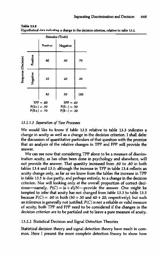
13.2.1.2 Change in the Decision Criterion

Table 13.5 shows, relative to table 13.3, a change in the decision criterion .We can say that the criterion has become more lenient because both TPPand FPP have increased, the former from .60 to .80 and the latter from .40to .60. Overall , the proportion of positive responses has increased, P(R + )

changing from .50 to .70, consistent with a change to a more lenient criterion for making a positive response.

648 Swets

Table 13.4

Hypothetical data indicating a change in disaimination acuity, relative to table 13.2.

Stimulus ( fruth )

Positive Negative

- ~c :c.9 .~ 40 10 SO1/1.~ ~Q-~ QIC >0 :c~ ~ 10 40 SO~ QI

Z

SO SO 100

TPP = .80 FPP = .20P(S+ ) = .50 P(S- ) = .50P(R+ ) = .50 P(R- ) = .50


Table 13.5Hypothetical

pO itivf

a J \H

!

SO

ddata indi~Hn~ a change in the decision criterion, relative to table 13.2.Stimulus (Truth)

40 30

10 20

TPP = .80 FPP = .60P(S+) = .50 P(S-) = .50P(R+) = .70 P(R-) = .30

Negative

(U

O! sp

aa

) asuo

dsa

' M

3 A

H

e S3

N

13.2.1.3 Separation of Two Process es

We would like to know if table 13.5 relative to table 13.3 indicates achange in acuity as well as a change in the decision criterion. I shall deferthe discussion of quantitative particulars of that question with the promisethat an analysis of the relative changes in TPP and FPP will provide theanswer.

We can see now that considering TPP alone to be a measure of discrimination acuity, as has often been done in psychology and elsewhere, will

not provide the answer. That quantity increased from .60 to .80 in bothtables 13.4 and 13.5; although the increase in TPP in table 13.4 reflects anacuity change only, as far as we know from the tables the increase in TPPin table 13.5 is due partly, and perhaps entirely, to a change in the decisioncriterion. Nor will looking only at the overall proportion of correct decisions

- namely, P(C) = (a + d)/N- provide the answer. One might betempted to infer that acuity has not changed from table 13.3 to table 13.5because P( C) = .60 in both (30 + 30 and 40 + 20, respectively), but suchan inference is generally not justified. P(C) is not a reliable or valid measureof acuity; both TPP and FPP need to be considered if the changes in thedecision criterion are to be partialed out to leave a pure measure of acuity.

13.2.2 Statistical Decision and Signal Detection Theories

Statistical decision theory and signal detection theory have much in common. Here I present the more complete detection theory to show how

discrimination and decision effects can be separated in detection, recognition, and diagnostic tasks.

13.2.2.1 Assumptions About an Observation

Signal detection theory incorporates three basic assumptions about an observation: (1) it can be represented as a value along a single dimension-

which we shall call the "decision variable," x- that reflects the likelihood

of stimulus A relative to stimulus 5; (2) observations of stimuli from either

category A or category 5 will vary from one observation to another inthe value of x they yield; and (3) values of x for observations from one

category will overlap those from the other category. Let us consider these

assumptions briefly.

ASSUMPTION 1: The observation is one-dimensional. The x value mightrepresent an observer's confidence that stimulus A is present as opposedto 5, as it does in mammography. Or it might be the amount of pressurein an eye as measured by an ophthalmologist screening for glaucoma. In a

simple sensory task, the idea of a single dimension may seem plausible:

detecting a spot of light might depend only on the rate of neural impulsesin certain brain cells. However, no matter how many dimensions anobservation may have- variations in a spot of light, for example, in hue,saturation, brightness, shape, duration, and so forth- the assumption ofdetection theory is that the only thing that counts is the likelihood of Arelative to 5 implied by the several dimensions taken together. If there areonly two possible responses, then, for purposes of making a decision, theobservation need have only one dimension; indeed, it should be reducedto one dimension if the best decisions are to be made.

ASSUMPTION 2: Observations of stimuli from either stimulus categorywill vary. It is clear that Xrays of breasts with either benign or malignantlesions will vary from one patient to another in the apparent likelihood of

malignancy. Some will show some particular signs of cancer and somewill show other particular signs, and more or less clearly. Similarly, samples

from each stimulus category in a sensory detection experiment willvary from trial to trial. For example, when observers try to detect theoccurrence of a faint tone within a background of white noise, the noise isinherently variable and the tone can also vary because the tone generatoris not perfectly stable. Even without such a noise background, essentiallyin quiet, the stimuli will appear variable to the observer because of naturalvariations in the observer's physiological, sensory system. Thus, auditorysensations affecting tone detection may result from the movements ofblood within the ear and visual sensations affecting light detection mayresult from variations in blood pressure within the eye. (See Wickens,chap. 12, this volume, for more discussion of sample variability and sample

distributions.)

650 Swets


ASSUMPTION 3: Values of the observation x &om the two categorieswill overlap each other . A background of white noise in a tone detectiontask has, by definition , energy at all audible &equencies, including the &e-

quency of the tone signal, and hence when the observer is attending narrowly to &equencies around the tone, the noise can produce observations

that sound like the signal . A malignant lesion may give little or no positive evidence in an Xray . A non liar in a polygraph exam may have a phys -

iological reaction as large as most liars. The overlap of observations will

vary &om small to large and discrimination acuity will vary accordingly .If there is no overlap , then no detection , recognition , or diagnostic problem

exists. This is because all x values produced by stimuli &om categoryA will be larger than any x values produced by stimuli &om category B,and an observer should have no difficulty discriminating between the twostimulus categories.

13.2.2.2 Distributions of Observations

Look ahead, please, to figure 13.7, which shows a representation of thethree assumptions as a pair of histograms labeled "0" and "3" on a decision

variable on the x-axis. You can ignore there the particular names ofthe decision variable , which we have generally termed x, and of the two

histograms . The histogram distributions may look more familiar if youimagine vertical lines &om each tick mark along the horizontal axis at thebottom up to the dashed and solid lines, respectively , of the two distributions

; then observations at each value of the decision variable are

represented by vertical bars. The height of a given bar represents the

probability that its value of x will occur . We see in accordance with

assumption 2 that the observations &om each stimulus category vary -

&om 2 through 12 for the stimulus category shown on the left ("category

B" as represented by the histogram labeled "0") and &om 5 through 15

for the category on the right ("A " or the "3"

histogram ). In accordancewith assumption 3, the observations &om the two categories overlap oneanother , such that the values 5 through 12 occur &om both categories .There is surety in this case for the extreme values 2 to 4 and 13 to IS , butsuch surety may not be evident in all cases.

To develop the analytical tools of signal detection theory , it is convenient to consider the distributions in a different form , namely , as continuous

probability distributions rather than as discrete histogram distributions .

Figure 13.2 shows a representation of the three assumptions as continuous

probability distributions on the decision variable x. Again , category B

gives rise to values of the observation x according to the distribution onthe left ; category A , according to the distribution on the right . Each valueof x will occur with a probability , when B is present, that is representedby the height of the B distribution at the particular value of x. And the

Figure 13.2.Probability distributions of observations. or of the decision variable x. for stimulus alternatives

A and B. with an illustrative decision criterion xc. and its corresponding areas orprobabilities FPP and TPP.

height of the A distribution, as one moves along the curve, gives the

probability that each value of x will occur when A is present.Readers familiar with the testing of statistical hypotheses will recall a

picture similar to that of figure 13.2, with the null hypothesis on the leftand an alternative hypothesis on the right . In signal detection theory, thetwo distributions are referred to as distributions of "noise alone" and"signal plus noise,

" respectively. This terminology arises for historical

reasons because with an electronic radar or sonar "signal," a stimulus from

category A is always viewed against a background of random interferenceor static called "noise,

" that is, a stimulus from category B. This noise maybe generated in the environment or in the detection device. In the case ofa human detector, as mentioned, noise results from the physiological vari-

ability inherent in sensory systems and in the nervous system in general.Thus, even though a stimulus from B is sometimes called a "null stimulus"

in a detection task, it is nevertheless a stimulus that impinges on theorganism, and one that may mimic, and be confused with, a stimulus fromA, or the signal. The occurrence of a signal adds something ("energy,

"

say) to the noise background; in general, values of x are larger for A orthe signal plus noise than for B or noise alone, and the distribution of xfor A is displaced to the right of the distribution of x for B. A good dealof data from the tasks of interest here indicates that these probability distributions

can reason ably, as well as conveniently, be considered as nor-

652 Swets.~:ctU.c Iea.....0~ ALTERNATIVE B ALTERNATIVE AcQ)~C"!u. xXcDecision Variable


mal (Gaussian) distributions , that is to say, as having the specific form ofthe bell -shaped distribution that is portrayed in the figure . Ordinarily ,however , despite their portrayal in figure 13.2, the distributions will havedifferent spreads or variances (e.g., the signal may add a variable quantity ,rather than a constant quantity , to the noise, and the signal distributionwill then have a wider spread). Clearly , discrimination acuity will dependon the separation of the two distributions : roughly speaking, the less

overlap , the less confusable are the stimuli . If, for example, the eye pressure test for glaucoma is perfectly acute, with pressure varying &om 30 to

50 physical units when glaucoma is present and &om 10 to 29 physicalunits in normal eyes, then there is no overlap and the two categories ofdisease and health will never be confused. If , however , the pressure test isnot very acute, for example, if glaucoma is associated with measurementsbetween 25 and 50 units and normal eyes with measurements between 10and 35 units , then overlap exists between 25 and 35 units and the diseaseand health categories will often be confused.

13.2.2.3 The Need for a Decision Criterion

In the face of such variability in observations and confusability in stimulus

categories, a rational decision maker will strive for whatever consistencyis possible . A basic kind of consistency is always to give the same response

to a given value of the decision variable . In other words , the decision maker will attempt to adopt , at least approximately , some particular

value of x as the decision criterion - call it xc- such that values of x

greater than Xc always lead to response A and values of x less than Xcalways lead to response B. In our mammography example, the radiologistwill choose some level of confidence that cancer exists (e.g., 5 on a 100-

point scale) and use it as consistently as possible for the decision criterion .

Figure 13.2 shows a somewhat conservative decision criterion Xc as avertical line on the decision variable and represents the probabilities oftrue positive outcomes (TPP) and false positive outcomes (FPP) that result&om that criterion . To see how this is so, consider how an observer whois being cautious about giving response A when response B is presentmight adopt the criterion shown , where most observations will be to theleft of the criterion , each one occurring with a relative &equency or probability

represented by the height of the B distribution at a given value ofx. But alternative B also produces values of x greater than xc- that is, tothe right of xc. The probability that a given value of x greater than Xc willoccur is represented again by the height of the distribution at that value .However , the probability that any value of x greater than Xc will occur is

given by considering the probabilities of those several values of x relativeto the total probability of all values of x. As I justify in a later discussion,the total area under the curve is taken to represent a probability of 1.0.

The probability that any value of x greater than Xc .will occur is equal tothe proportion of the total area under the curve that lies to the right of xc.

Specifically , FPP is equal to the proportion of the area under curve B tothe right of Xc and TPP is equal to the proportion of the area under curveA to the right of xc, as shown by hatch lines. Both probabilities willincrease for more lenient criteria - as Xc moves to the left - and decreasefor stricter criteria - as Xc moves to the right . (Though not labeled in

figure 13.2, the proportions of area to the left of the decision criterion Xcrepresent the two decision probabilities that are complementary to FPPand TPP, respectively : the true negative proportion under curve B and thefalse negative proportion under curve A .)

13.2.2.4 Decision Criterion Measured by the Likelihood Ratio

One general way to measure the location of the decision criterion -

independent of a particular decision variable , be it a mammographer's confidence

or the opthamologist's physical measure of pressure in the eyeis

by the quantity called " likelihood ratio " (LR). The LR at any value of X

of the decision variable is the likelihood that this value of x came fromdistribution A relative to the likelihood that it came from distribution B.In terms of figure 13.2, it is defined as the ratio (at that value of x) of the

height of the A distribution to the height of the B distribution . Thus, for

example, the LR is 1.0 where the two curves cross. As seen in figure 13.2,the LR for a decision criterion increases (toward infinity ) as the criterionmoves to the right and decreases (toward zero) as the criterion moves tothe left . (If the two distributions have unequal spreads, the two curves willcross a second time out at one or the other tail , but we shall ignore suchend effects for present purposes.) As one specific example, observe that in

figure 13.2 the illustrative criterion Xc is set at the midpoint of the righthand distribution , where the height of A happens in this picture to be a

little more than twice the height of B. More precisely , the LR at that pointis 2.5. Other measures of the decision criterion have been considered; an

advantage of LR, as we shall see next , is that it facilitates definition of thebest, or the "optimal ,

" criterion for any specific task. Let us denote acriterion value of LR as LRc.

13.2.2.5 Optimal Decision Criterion

In most tasks, particularly in diagnostic tasks, an observer /decision makerwill want to choose a location of the decision criterion that is best for some

purpose . In the mammography example, one desires an appropriate balance between the proportions of false positive and true positive responses,

FPP and TPP. This is because FP outcomes have significant costs and TPoutcomes have significant benefits; similarly with the other two stimulus -

response outcomes : false negative (FN) outcomes have costs and true

654 Swets


LRc = ~~~ x benefit(TN) - cost(FP)P(S+ ) benefit(TP) - cost(FN)

.

That is, the expected value optimal criterion is specified by an LRc definedas a ratio of the prior probabilities and a ratio of benefits and costs. (Because

the costs are negative, one adds the absolute values of the benefitsand costs.) How benefits and costs may be assigned to decision outcomeswill be di~nJ~~pd lal-pr

In this way, any set of prior probabilities, benefits, and costs determinesa specific criterion value Xc, in terms of LRc, that is best for that set ofvariables. It is best or optimal because it maximizes the payoff to thedecision maker.

Note that the negative alternative is represented in the numerator ofthe probability part of the equation, P(S- ), and also in the numerator of

negative (TN ) outcomes have benefits. Further , the proportions of the

positive and negative stimuli , which we have denoted P(S+ ) and P(S- ),will affect the location of the best criterion . We shall discuss this relationlater, but you can see now that if P(S+ ) is high - if , for example, in acertain

breast-cancer referral setting , most of the patients seen have a malignancy- one would do best to reflect that high P(S+ ) in a high proportion

of positive responses, P(R + ), and a lenient criterion toward the left of

figure 13.2 is needed to produce a high P(R+ ). Conversely , a lowP(S+ )- as in mammography screening of nonsyrnptomatic women - isbest served by a low P(R + ), which requires a strict criterion toward the

right of figure 13.2.An optimal decision criterion can be defined quantitatively in various

ways . One very useful definition of the optimum is based, as discussed, onthe prior probabilities of the two stimuli , P(S+ ) and P(S- ), and the benefits

and costs of the four decision outcomes, TP, FP, FN, and TN , shownin table 13.1. This criterion is called the "

expected value" criterion because it maximizes the "mathematical expected value" of a decision - or

the net result of the benefits and costs that may be expected on averagewhen this criterion is used for many decisions (Peterson, Birdsall , and Fox1954; Green and Swets 1966). Specifically , if we multiply the benefit orcost of each of the four possible outcomes by the probability of that outcome

(a I N , biN , etc., in table 13.2), and add these four products , we obtainthe expected (or average) value of the decision . (In this calculation , costsmust be taken as negative .) It is desirable to maximize that value overmany decisions because then the total benefit relative to the total cost is

greatest .

Although a fair amount of algebra is required , which we shall bypass, itcan be shown that the expected value is maximized when a criterion valueof LR, that is, LRc, is chosen such that

the benefit -cost part . Similarly , the denominators in both the probabilityand benefit -cost parts represent the occurrence of the positive alternative .Thus, for a fixed set of benefits and costs, the optimal LR, will be relatively

large - and the criterion will be relatively strict - whenever P(S- )is appreciably greater than P(S+ ). That is, one should not make the positive

decision very readily if the chances are great that the negative alternative will occur. If, instead, the prior probabilities are constant and the

benefits and costs vary , the optimal LR, will be large and the optimal criterion will be relatively strict when the numerator of the benefit -cost part

of the equation is large relative to its denominator , that is, when more

importance is attached to being correct in the event the negative alternative occurs. Such might be the case when a surgical technique inquestion

has substantial risks and its chances of a satisfactory outcome arelow . Conversely , the optimal LR, will be small and the optimal criterionwill be lenient when the benefit -cost denominator is large relative to itsnumerator , that is, when it is more important to be correct when the positive

alternative occurs. Such is the case in deciding whether to predict asevere storm .

13.2.2.6 A Traditional Measure of Acuity

if a decision criterion value x, is placed midway between two distributions and the separation between the two distributions is increased, the

TPP will get closer and closer to 1.0 while the FPP is getting closer to O.Thus, as can be seen in figure 13.2, one way to measure discrimination

acuity is to measure the difference , or distance, between the midpoints ormeans of the two distributions . In some tasks, the distributions are available

themselves from data; in tasks for which they are not , this measurecan be inferred from measured values of FPP and TPP. Usually , the difference

between the means is divided by the standard deviation of one of thedistributions - as a measure of the spread of the distribution - and therefore

is measured in the units of that standard deviation . (See Wickens ,

chap. 12, this volume , for a discussion of the standard deviation of a distribution.) If the two distributions have the same standard deviation ,

which I have said in practice they usually do not , then this measure iscalled d'

(read "d-prime"). I mention d' here because it is ingrained in psychological

uses of signal detection theory . Indeed, the LR, criterion valuehas been termed p (

"beta ") and the phrased -prime and beta" is used

often as shorthand to signify separation of the discrimination and decision

process es in psychology . Other discrimination measures have been defined and used that are variants of d', which are appropriate when the two

distributions differ in spread. Section 13.3 defines a measure I believe tobe preferable, and incidentally one that is commonly used in diagnostictasks.

656 Swets

1 . 0

0 . 9

LENIENT

/

CRITERION

/

0 . 8

/MODERATE

0 . 7 CRITERION

/

0 . 6 /

/

0 . 5

STRICT

/

CRITERK > N

0 . 4

/

0 . 3

/

/

0 . 2

/

0 . 1

/

0

. . . . . . . . . 9 1 .1

NO

IJ. } J O

d~ d 3t \ 1J . I S

Od

3n ~ J .

PROPORTION

Relative OperatingCharaderistic

A simple and compact, graphical way of quantitatively separating discrimination and decision process es is the "relative operating characteristic"

(ROC). The ROC is a plot of TPP versus FPP, for a given acuity, as thedecision criterion varies (Peterson, Birdsall, and Fox 1954). Given a strict(high) criterion corresponding to an Xc criterion toward the right side offigure 13.2, both proportions are near 0; given a more lenient (low) criterion

corresponding to an Xc value to the left in figure 13.2, they bothapproach 1.0. Figure 13.3 shows an idealized ROC as a curve of decreasing

slope running from 0 to 1.0 on each axis. It identifies three arbitrarilyselected (TPP, FPP) pairs along the curve, each corresponding to adifferent

possible decision criterion.Note that if the ROC fell along the dashed, diagonal line, it would represent

zero acuity: everywhere along this line TPP is equal to FPP, whichis a result that can be obtained by pure guesswork or chance in choosingbetween categories A and B, without making an observation. As acuityincreases, the ROC moves away from the diagonal, in a direction leftwardand upward toward the upper left comer of the graph, where acuity is

Separating Discrimination and Decision 6S 7

FALSE POSITIVE

Figure 13.3

13.3 The

The relative operatin~ maraderistic (ROC), with three nominal decision criteria.

perfect: TPP = 1.0 while FPP = o. Hence a suitable measure of acuity willreflect the distance of the ROC from the diagonal line. For a particularlevel of acuity, a given decision criterion produces a particular data pointalong the ROC's curve and so a suitable measure of the criterion will represent

the location of that point along the curve. The purpose of the ROCis to measure discrimination acuity independent of any decision criterionby displaying discrimination data at all possible decision criteria.

13.3.1 Obtaining an Empirical ROC

To obtain an empirical ROC for any observer or device at a particularlevel of acuity, sufficient data points (each corresponding to a differentdecision criterion) are obtained along the curve to fit the curve adequately

, that is, to determine quite reliably just where the curve lies. Five

points, each based on 100 or so observations, are usually thought to besufficient. One way to obtain these points is to vary from one group oftrials to another some variable or variables that will induce the observerto adopt a different criterion for each group of trials. Thus one could

vary the prior probabilities of the stimuli A and B, or the benefits andcosts (rewards and penalties) of the decision outcomes, or both, and defineone ROC data point for each particular case. In such an experiment, theobserver makes a choice between the two alternative responses, A and Bin our general terms. In a signal detection problem, the response is either"yes

" (a signal is present) or "no"

(no signal is present) and the two-

response method is often called the "yes-no method."

A more efficient way of obtaining data points on an empirical ROC isthe "rating method," in which the observers rate their confidence (e.g.,on a six-category scale) that stimulus A is present. Here, the observerchooses among multiple responses, six in this example, and the experimenter

regards these different confidence responses as resulting from thesimultaneous adoption of a set of different criteria. Specifically, if anobserver establish es five different decision criteria, the decision variable isdivided into six regions, each corresponding to one of the six possibleresponses. Then, in analysis, the experimenter treats different responses as

representing different decision criteria. In figure 13.2, you could picturefive vertical lines (corresponding to five values of xc) spread across thedecision variable. To illustrate, let us follow the convention that a ratingof 1 indicates the highest confidence that alternative A is present, and 6,the lowest. Thus a rating of 1 corresponds to a very strict criterion (an Xcto the right in figure 13.2) while a rating of 6 corresponds to a very lenient

criterion (an Xc at the left in figure 13.2.) The data analyst first takes

only ratings of 1 to indicate a "yes"

(or positive judgment) and calculatesa data point (FPP and TPP) based on them. This point represents thestrictest criterion used by the observer. Next, the analyst takes ratings of

658 Swets

both 1 and 2 to indicate a positive judgment and calculates a data pointbased on them. This is the second strictest criterion used by the observer.And so on for ratings 1, 2, and 3, ratings 1, 2, 3, and 4, and, finally, forratings 1, 2, 3, 4, and 5- the rating of 6 is never included as a positiveresponse, because then all responses would be positive and the trivial datapoint at the upper right comer (FPP = 1.0, TPP = 1.0) would result. Inthis way, progressively more rating categories are treated as if they werepositive responses and progressively more lenient criteria are measured.In performing under the rating method, the observer adopts several criteria

simultaneously- rather than successively in different groups oftrials- and thereby provides an economy in data collection.

Separating Discrimination .and Decision 659

13.3.2 A Measure of the Decision Criterion

Although the ROC of figure 13.3 is shown with three possible decisioncriteria, in theory, the criterion can be set anywhere along the decisionvariable. Hence, if the decision variable is scaled finely enough to be essentially

continuous, the ROC will be essentially continuous. One might,for example, ask an observer to make a probability estimate that stimulusA is present, that is, to use a 100-category rating scale, and therebyachieve an approximately continuous ROC.

As remarked earlier, a criterion corresponds to, and can be measuredby, a value of likelihood ratio. Recall that the criterion value LR, is theratio of the heights of the two probability distributions at any given valueof the decision variable, x, (figure 13.2). It can be shown that the value ofLR, is also equal to the slope of the ROC at the data point that is produced

by that criterion LR,. (Strictly, it is equal to the slope of a line tangent to the ROC at the data point.) Thus very strict criteria to the right in

figure 13.2, with high values of LR" produce a point on the ROC wherethe slope is steep- at the lower left of the graph. A moderate criterion,LR, near 1.0, produces a point near the middle of the ROC. A very lenientcriterion, to the left in figure 13.2, yields an ROC point where the slope isapproximately flat, near 0, at the upper right . This slope measure of thedecision criterion is denoted 5 (rather than LR,) in our further discussion.Two illustrative values of 5 are illustrated in figure 13.4: 5 = 2 for a relatively

strict criterion and 5 = 1/ 2 for a relatively lenient criterion. Thecalculation of the slope measure is illustrated with data in section 13.5.

13.3.3 A Measure of Discrimination Acuity

Figure 13.5 shows ROCs representing three possible degrees of discrimination acuity. As mentioned, the range of possible ROCs runs from the

dashed diagonal line (where TPP = FPP and hence acuity is zero anddecisions are correct only by chance) to a curve that follows the left andtop axes (where acuity is perfect, TPP = 1.0 for all values of FPP). Thus it

1 .

.

.

. "

"

. 6 "

"

. 5

. 3

. 2

S=

SLOPE INDEX

. (Two Illustrative Values

)

0 . 1 . 2 . 3 . . 5 . 6 . 7 . 8 . 9 1 . 0

Figure 13.4The relative operating characteristic (ROC) with two i Uustrative values of the slope measureof the decision criterionS .

is evident that the proportion of the graph's area that lies beneath the

ROC is a possible measure of acuity. This area measure ranges from a lowvalue of .50 (for an ROC lying along the "chance" diagonal, where half ofthe graph

's area is beneath the ROC) to a high value of 1.0 (for an ROC

running along the left and upper axes of the graph and subtending all ofits area). When normal distributions are assumed, as in section 13.2 above,the area measure is denoted Az' because the units along the horizontalaxis of the normal distribution are called "z scores." Figure 13.6 showssome illustrative values of Az.

It may help to provide some intuitive grasp of the values of this areameasure to know that it is equal to the proportion of correct choices in a"paired-comparison

" task- in which alternatives A and B are presentedtogether: in each observation and the observer says which is which. For

example, a radiologist might be shown two Xrays and would have to saywhich shows the malignant condition. If the radiologist were correct 95

percent of the time in such a paired-comparison task, the yes-no or ratingmethod would yield the top curve (Az = .95) in figure 13.6 (Green andSwets 1966).

660 SwetsN

OI

. l Y

Od

O

Yd

3AI

. lISO

d

3ny

. l

FALSE POSITIVE PROPORTION

. . . . . - - -

OU

~ OdO

~ d 3 A

U

I SO

d

3n ~ 1


A measure of acuity drawn from the ROC is independent of any decision criterion that might be adopted; it reflects all possible decision criteria. I emphasize now that such a measure is also independent of the

prior probabilities of the two stimulus alternatives that may inhere in anyparticular situation because it is based on the quantities FPP and TPP,which are independent of the prior probabilities- as shown in table 13.2and related text. For example, changing P(S+ ) will change the columnsum a + c in table 13.2, but does not change TPP = a/(a + c). Hence anROC acuity measure is a general measure of the fundamental capacityfor discrimination and it represents the full range of situations in whichthat particular discrimination might be called for. It is not specific to, ordependent on, any of one them.

13.3.4 Empirical Estimates of the Two Measures

I merely note that it is possible to obtain graphical estimates of the criterion measureS and of an area measure of acuity, as when successive data

points in the ROC space are connected by straight lines. In this case, theslopes of connecting lines between points give the criterion measure 5 foreach successive point (specifically, the slope of the line connecting two

1.0

0.9

0.8

0.7

0.6

0.5

0.4

0.3

0.2

0.1

0- - - --- --- --- --- -.0

FALSE POSITIVE "PROPORTION

Figure 13.5The relative operating characteristic (ROC) at three nominal levels of disaimination acuity.

1 . 0

Z

. 9

0

~

. 8

a : :

0

Q . .

. 7

0

a : :

Q . .

. 6

w

> . 5

t :

( / ) . 4

0

Q .

. 3

. 2

. 1

0

0 . 1 . 2 . 3 . 4 . 5 . 6 . 7 . 8 . 9 1 . 0

13 .4 Illustrations of Decomposition of Disaimination and

There follow five examples in which the ROC analysis was used to separate the two behavioral process es of interest , two examples from psychol -

662 Swets

1AJ:)Q:...


Figure 13.6The relative operating characteristic (ROO at some illustrative values of the measure of discrimination

acuity, Az.

points gives 5 for the higher point). The area beneath that ROC can bemeasured graphically by adding up the areas in the trapezoids formed bydropping vertical lines from the data points. In practice, however, acom-

puter program is used to fit smooth curves to ROC data and to calculatethe two measures along with estimates of their statistical variability (Swetsand Pickett 1982).

It should be clear now how the ROC indicates observed changes in behavior to be discrimination effects or decision effects, or both. If the entire

curve moves in the direction of the dashed diagonal line in figure 13.6,that is, moves to contain more or less area beneath it, then there is a discrimination

effect, whether or not there is a decision effect as given by themeasureS. If a data point (or set of points in the rating method) moves

along a given curve, then there is a decision effect. The quantitative measures

give the sizes of such effects.

Decision

ogy and three from practical diagnostic tasks.

Outside the laboratory , signal detection must often be accomplished during a long observation period with in&equent signals occurring at random

times. Such is the case in military contexts , where the problem may be todetect the approach of an enemy plane, and in industrial inspection , wherethe problem may be to detect defective products on an assembly line .Since such in&equent, random signals have been studied in the laboratory ,beginning in about 1950, it has been found consistently that the true positive

proportion falls off notice ably in only a half hour of observation - afinding suggesting that enemy planes and faulty products will likely bemissed (Mackworth 1950; Mackle 1977). Investigators asked whether thisfinding could reflect a decrement in discrimination acuity due to fatigueor inattention , even though the time course of the decrement was veryshort . Hundreds of studies over several years examined variables thoughtto affect fatigue and alertness, including work -rest cycles, intersignal interval

, irrelevant stimulation , incentives , knowledge of results, introversion -extroversion , temperature , drugs , age, and sex (Buckner and McGrath1963; Broadbent 1971). At least five theories were proposed to accountfor a decrement in acuity (Frankmann and Adams 1962).

Then, led by James Egan (Egan, Greenberg , and Schulman 1961) andDonald Broadbent (Broadbent and Gregory 1963), investigators beganto ask whether the drop in the TPP reflected instead a change in the decision

criterion . Might observers be setting a stricter criterion as time progressed- that is, requiring stronger evidence to say that a signal waspresent--: conceivably because their estimate of the prior probability ofsignal occurrence was going down as they experienced signals at a lower -than-expected rate? If so, the FPP (as well as the TPP) should bedecreasing

over time . False positive responses were then tallied and found to bein fact decreasing. Another hundred or so studies have since shown thatfor most stimulus displays , the principal , and sometimes only , changeover a vigil is in the decision criterion . .

Under some rather special conditions , changes in acuity are regularlyfound , as well as changes in the criterion . For example, a change in acuityis found when a discrimination must be made between two stimulus alternatives

presented successively, which puts a greater demand on memorythan a discrimination between simultaneous stimuli . A high rate of stimulusoccurrence also produces a decline in acuity , perhaps because it requirescontinuous observation , which may be difficult to maintain (Parasuramanand Davies 1977).

Given the tendency for the criterion to change as the main effect, however, task design has shifted to controlling it : Military commanders would

like their observers to use consistently a criterion that reflects realistically


13.4.1 Signal Detection during a Vigil

the prior probability of attack and the benefits and costs of alternativedecision outcomes; similarly, manufacturers would like their inspectors to

employ a criterion that satisfies management's objectives for the quality

of the product (Swets 1977).

664 Swets

13.4.2 Recognition Memory

In a typical laboratory recognition memory task, the subject is asked to

say whether each of a series of items (e.g., a word ) was presented before

("old

") or not (

"new"). Applying signal detection theory to obtain a pure

measure of "memory strength ,

" analogous to acuity , depends on the assumption

that all items lie along a continuum of strength , with the strengthof each item being determined by conditions of memorizing and forgetting

(Murdock and Duffy 1972). The subject sets a decision criterion on

the strength continuum to issue a response of "old ," and the investigator

attempts to separate actual phenomena of memory from decision or response

process es that may vary within and across subjects for reasons independent

of memory (Egan 1958).Several experimental effects that were presumed to reflect memory

strength were later shown to be effects of the decision criterion instead

(Swets 1973). These effects include the apparently better recognition of

more common words - in fact, there is evidence that recognition memoryis better for uncommon words (Broadbent 1971); the differences in recall

of familiar and unfamiliar associations (McNicol and Ryder 1971); the

buildup of false responses of "old " during a continuous recognition task

(Donald son and Murdock 1968); effects of interpolated learning (Banks

1969); changes in semantic or association context from acquisition to recall

(Da Polito , Barker, and Wiant 1971); and gender differences (Barr-Brown

and White 1971). Effects due both to memory and decision process es

were found for meaningfulness of items (Raser 1970), serial position(Murdock 1968), and the similarity of distractor items (Mandler , Pearl-

stone, and Koopmans 1969). A study of elderly patients , including both

demented and depressed individuals , showed that an apparent memoryloss that seemed similar for both types of patients was, in fact, a true

memory impairment for demented individuals , but rather a criterion

(confidence or caution ) effect for depressed individuals (Miller and Lewis

1977).

13.4.3 Polygraph Lie Detection

Attempts to detect individuals who are lying about certain events- by

examining the various physiological measures (such as heart rate) that are

taken by a "polygraph

" machine- aTe increasingly being made both in

court cases and in employment settings where security is important (Saxe,


13.4.4 Information Retrieval

Conventional library systems manually retrieve documents from shelvesand facts from documents by means of familiar card indexes based oncataloguing methods. Computer-based retrieval systems scan documentselectronically, looking for various properties of the text- for the appearance

of key words, say- and give the documents a relevance score torepresent how likely they are to contain wanted information. In bothcases, a decision criterion must be established: how likely must the document

be to satisfy the specified need for information in order to proceed

Dougherty, and Cross 1985). According to a recent article, the need toseparate discrimination acuity and the decision criterion is simply notappreciated in this field:

Despite lengthy congressional hearings conducted during the preparation of the Employee Protection Act of 1988, no one ever explained the distinction between accuracy [acuity] and a decision

criterion to the legislators. Thus, the policy makers never learnedabout a polygrapher

's predilection to err on the side of false positives or false negatives, constancy in the location of his or her decision

criterion, or ability to change his or her decision criterion.Individual differences among polygraphers with respect to theirdecision criteria thus remain unknown, and persons appearingbefore a polygrapher are- unknowingly- up against the "luck ofthe draw." (Hammond, Harvey, and Hastie 1992, 84).

Studies have shown polygraphers to have widely different acuitiesand also quite different decision criteria for accusing a person of lying(Shakhar, Lieblich, and Kugelmass 1970; Szucko and Kleinmuntz 1981).However, there is a general tendency toward a lenient criterion for concluding

that an individual is lying, probably because accusations hold achance of eliciting a confession. In this respect, polygraphers may careless about their technique

's acuity if it is effective in eliciting a confessionnow and then. As a consequence, the ratio of persons falsely accused tothose truly accused is often quite high- in some studies, as high as 20 to1 (Szucko and Kleinmuntz 1981). As attempts are made to expand thedomain of polygraphy, we can ask, should the criterion for accusation bedifferent for security screening in the workplace than for criminal cases?Specifically, how do the prior probabilities, and especially the benefits andcosts, differ? Polygraphers find it rather easy to change their decision criteria

; as in mammography, they look for certain perceptual features of therecording of physiological variables and can adjust the decision criterionexplicitly by requiring the presence of more or fewer of these features.

to retrieve it for further examination? The decision criterion might be

specified for computer systems in terms of the number of key words adocument must contain or in terms of how high its relevance score mustbe. Here again, librarians considering alternative systems for use shouldknow the relative acuities of the systems- how well they separate thewheat from the chaff- independent of any particular decision criterion.Users will want to set a criterion to individual likings when the system isin operation. In examining the retrieval performance of several alternative

systems with the relative operating characteristic (ROC) technique, Ifound that their various approach es to the scoring of relevance led to

only negligible differences in acuity (Swets 1969). As examples of different

approach es, one system might consider only specified key words,whereas a second might also consider synonyms of the specified keywords; a third system might scan the full text, and a fourth, just theabstract.

Incidentally, the typical acuities found suggest that the retrieval problem is more difficult than we might have thought. Consider a file of 3,000

documents and assume that for each query to the file 10 documents are

actually relevant. To retrieve 3 of the 10 relevant documents, one must

accept, on average, 3 false positives, that is, 3 unwanted, irrelevant documents. To retrieve 6 of 10 relevant items, a more lenient criterion must be

effected, and then 30 false positives will occur. A user desiring to retrieve9 of the 10 relevant documents will have to set a very lenient criterionand then will have to winnow the 9 relevant documents from the approximately

300 retrieved, some 290 of which will be just "noise."

13.4.5 Weather Forecasting

666 Swets

Ian Mason (1982a) first applied signal detection theory to predicting various kinds of weather events. Weather forecasting represents a diagnostic

problem similar to information retrieval, medical diagnosis, materials testing

, and so forth, in that we want to measure acuity independent of thedecision criterion when alternative systems (or "models") for forecastingare being evaluated prior to selecting one of them for use, and then wantto adjust the criterion to an appropriate level when the selected system is

operating in actual practice. Mason showed that predictions of variouskinds of weather give data that are fitted well by the ROC. He showedfurther (1982b) that the several existing (non-ROC) measures of acuityused in this field confound discrimination acuity and the decision criterionand hence give unreliable measures of acuity.

Weather forecasters have recognized the operational problem of settingdecision criteria in recent years by giving probability estimates for weatherevents, thus permit ting the forecast user to set his or her own decision


criterion . The orange grower can decide, in terms of personal costs andbenefits, whether the likelihood of frost is high enough to set out thesmoke pots . You and I can decide whether or not to carry an umbrella .

13 .5 Computational Example of Decomposition : A Dice Game

A deep understanding of the theory discussed above comes quite easily byway of a game (Swets 1991a). In the game, three dice are thrown repeat-

edly. Two are ordinary dice with 1 through 6 spots on the six sides; thethird die has 3 spots on each of three sides and blanks on the other threesides. For each throw, you are given the total number of spots showing-

your observation- and you must say whether the unusual die showed a 3(positive event) or a 0 (negative event). You win $1 on true positive andtrue negative outcomes and lose $1 on false positive and false negativeoutcomes. I assume that you will set a decision criterion at some particularnumber of spots and consistently respond

"3" when and only when thatnumber is met or exceeded. The optimal criterion is the one that maxi-mizes your payoff and you will want to determine that number.

13.5.1 Distributions of Observations

Consider the initial steps in determining the optimal decision criterion.You need first to calculate the distributions of observations under eachstimulus alternative: the probability of each of the possible totals 2 through12 when the third die shows a 0 and the probability of each of the possible

totals 5 through 15 when the third die shows a 3. So you constructtable 13.6 to show the number of different ways in which each total 2

through 12 can occur on two ordinary dice- relevant to throws on whichthe third die shows a O. Reading along the positive diagonals from lowerleft to upper right, you note that a total of 2 can occur on the two ordinary

Table 13.6Pnccihlp .hrnwc whpn .hird dip ~hnw ~

2 3 4 5

1 2 3 4 5 6 7

2 3 4 5 6 7 8

Number of

spots

3 4 5 6 7 8 9

showing

on

d di

4 5 6 7 8 9 10

seton e

5 6 7 8 9 10 11

6 7 8 9 10 11 12

��

Number of spots showing on first die

dice in only one way (I , I ), a total of 3 can occur in two ways (I , 2, and 2,I ), and so on. Because there are 36 different kinds of throws possible, the

probability of a 2 (which can occur one way ) is 1/36 (or .028), the probability of a 3 (which can occur two ways ) is 2/36 (.056), and so forth . The

appropriate table for the throws on which the third die shows a 3 is

obtained by adding 3 to each cell entry in table 13.6; these values are

shown in table 13.7.You will need table 13.8, which lists the number of ways in which each

total can occur when a 0 shows (column 2) and when a 3 shows (column 3)and also the probability of each total given a 0 (column 4) and given a 3

(column 5). Just as the numbers of ways a given total can occur (for 0 and

3, respectively ) add up to 36, so the probabilities (for each of the two

types of throw ) add up to 1.Now you can construct the two probability distributions - as histo -

grams because your observations are of integer values only ; that is, theyare discrete rather than continuous . These distributions are shown in figure

13.7, where the distribution for throws of 0 is on the left (dashed line)and the distribution given a 3 is on the right (solid line). In earlier termi -

no logy , the totals of the two ordinary dice constitute the "noise" of signaldetection theory , and the third die either adds a signal to the noise or

does not . This dice game provides more surety than many more realistic

tasks in that certain observations very clearly and definitely come from

one or the other stimulus alternative . Specifically , in this case, there is no

uncertainty or decision problem for the totals 2 to 4 (which definitelyindicate a 0) or the totals 13 to 15 (which definitely indicate a 3).

Following up on our earlier discussion of continuous probability distributions in figure 13.2, picture vertical lines in figure 13.7 extended from

each tick mark on the horizontal axis up to the dashed and solid lines, so

that each total of the three dice (under each of the alternatives 0 and 3) is

represented by a vertical bar. If the bars are assumed to have a width of

668 Swets

Table 13.7Possible throws when third die shows 3

12345

789

10

89

9101112

10111213

II121314

Number of spotsshowing onsecond die

789

�

Number of spots showing on first die�

1 2 3 4 5 6

5 6 7 8 9 106

6 10 11 12 13 14 151011

Note: Columns 2 and 3, respectively, are the numbers of ways each total number of spots aslisted in column 1 can occur when a 0 is thrown, and when a 3 is thrown, on the third die;columns 4 and 5 are the corresponding probabilities for each total listed in column 1; column6 is the likelihood ratio for each total listed in column 1, namely, the ratio of column 5 tocolumn 4; the FPP in column 7 is the probability of observing a total number of spots that isat least as great as the value in column 1, given that a 0 shows on the third die; similarly, theTPP in column 8 is that probability given a 3 showing on the third die.


Table 13.8Probabilities of the various totals, the likelihood ratio, and the ROC coordinates.�

one unit, then the area of a bar (as well as its height) reflects the probability of its corresponding total of the three dice. Because the probabilities

for each histogram add up to 1, the total area under each histogram equals1. Hence we can add the areas of the bars to the right of a decision criterion

, for the left and right histograms, to give the probabilities FPP andTPP, respectively. This operation may help you to understand the wayareas yield FPP and TPP for the continuous distributions of figure 13.2.

13.5.2 The Optimal Decision Criterion for the Symmetrical Game

What total of the three dice do you choose for your decision criterion?The answer is straightforward for this symmetrical game-

"symmetrical

"

in the sense that the chances of a 0 and 3 are equal (there are three of eachon the third die) and all benefits and costs are equal. Here we need only todetermine which totals are more likely when a 3 occurs on the third die

Likelihood Ratio

0 00 0000

. 167 r

- -

'

I I

I I

. 139

O

~

_ - J

. 111 r

- - - ' - -

. ,

I

I

I I

. 083 r

- - ' " 1 . . _ -

,

I I

I I

. 056 , .

- _ J ' - - -

,

I I

I I

. 028

- _ J L _ _

,

I

0

2 4 7 8 9 10

Total of Three Dice

9: > U

9JJn

: > oo

10

AJ

! I ! qeqO

Jd

670 Swets

Figure 13.7Histograms of the probabilities of occurrence of the totals of three dice (for the odd dieshowing 0 on three sides and 3 spots on three sides), with the likelihood ratio for each total.

than when a 0 occurs and, conversely, which totals are more likely for a 0than a 3. According to table 13.8, totals of 9 and greater are more likelyfor a 3 than for a 0, and totals of 8 or less are more likely for a 0 than for a3. If you think of the optimal criterion then as 8.5, you can note in figure13.7 that it occurs exactly in the middle of the pair of histograms, that is,where they

"cross" each other. This result is intuitively proper for a symmetrical game.

Would you rather play the game when the third die has 4 spots on threesides instead of 3 spots? For this new version of the game, the histogramsare further apart and so your acuity will be higher, and the decisionsshould be better and produce a higher payoff. Specifically, the right-hand

histogram moves one unit to the right . ( Now the total of 5 is a sure signof a 0, along with totals of 2, 3, 4, and the new possible total of 16 is asure sign of a 4, along with totals of 13, 14, 15.) Because the optimal criterion

also moves one unit to the right, to 9.5, here you say "4" for

totals ~ 10.

13.5.3 The Optimal Decision Criterion in General

Returning to the first version of the game, with 0 or 3 spots, what now ifthe third die shows 3 spots on four sides, rather than three? Or on twosides rather than three? How do such changes in the prior probabilitiesaffect the optimal criterion? Given our earlier discussion (in section

13.5.4 The Likelihood Ratio

To use this result, you need to know the value of the LR for each totalnumber of spots. Table 13.8 shows the values of the LR in column 6; theyare the ratios of values in column 5 (probability of a given total if 3occurs) to those in column 4 (probability of a given total if 0 occurs)- justas we defined the LR earlier in terms of heights of continuous distributions(section 13.2.2.4). You note in table 13.8 that with an LR criterion of .20,


13.2.2.5), you respond that having 3 spots on four sides leads to a morelenient criterion, whereas having 3 spots on two sides leads to a strictercriterion (than 8.5).

Further, consider a change in benefits and costs: say that the TN and FPoutcomes (possible when the third die shows a 0) remain at +$1 and - $1,respectively, but that the TP and FN outcomes (possible when the thirddie shows a 3) become +$5 and -$5, respectively. Because :t:$1 applieswhen a 0 occurs on the third die and :t: $5 applies when a 3 occurs, it ismore important to be correct when a 3 occurs, and you will want to say"3" more often, by setting a lower criterion number of total spots (lowerthan 8.5). To determine just what that criterion number is, we need toemploy the formula for the optimal, expected value criterion presentedearlier in terms of the likelihood ratio criterion, LR" in section 13.2.2.5. Itis an "expected value" (EV) criterion you want because you want to maximize

your average payoff over many plays of the game arid that is whatthe EV is.

Again, to avoid a fair amount of algebra, we shall go through the operations of this example only in summary. First you multiply the probabilityof each outcome by its value (benefit or cost) to obtain its EV, and thenyou add the two EVs for each possible decision (0 or 3) to get each deci-sion's EV. At this point, were you to make some algebraic substitutionsand collect and rearrange some terms, you would find that if you choose 3for those totals having a higher EV for 3 than 0 (and choose 0 for theother totals), you will be saying "3" whenever the LR of a total is greaterthan LR" where

LR, = ~ x benefit (TN) - cost(FP)P(3) benefit(TP) - cost(FN) ,

which is identical to the formula given in section 13.2.2.5. (As notedbefore, a cost has a negative value; hence the absolute values of benefitand cost are added.) For the game at hand, where the benefits and costsare :f: $1 and :f: $5, you say

"3" when the LR exceeds

.5 1 + 1 2- X = - = .20.

.5 5 + 5 10

you say "3" for totals of 5 or more - as it happens here whenever the

probability of 3 exceeds zero.The LRs listed in table 13.8 are printed along the top of figure 13.7

where they indicate the ratios of heights of the histogram bars (the ratioof 3's heights to O's heights) at each three-dice total. If you draw a verticalline there, to represent LR = .20, at the tick mark between 0 and .25, andextend it down to the bottom axis, you see again that an LR criterion of.20 leads to saying

"3" whenever the total is 5 or more (greater than 4.5).

13.5.5 The Dice Game's ROC

To construct the game's ROC, we must know the probabilities for TP and

FP for each decision criterion. I designate these probabilities as I did their

proportions, TPP and FPP. We can calculate the relevant probabilities byapplying the ideas used in the rating method introduced in section 13.3.1.

They are shown in columns 7 and 8 of table 13.8. Note that in this table,the criteria &om top to bottom (2 spots to 15 spots) run &om lenient tostrict, and thus, to maintain the convention of section 13.3.1, where westarted cumulating probabilities at the strictest criterion, we begin cumulating

&om the bottom of the table. For illustration, consider first the prob-

abilities of various numbers of total spots showing when a 0 occurs onthe third die- in column 4- and the corresponding values of FPP for criteria

set at those different numbers of total spots- in column 7. Reading&om the bottom of column 4, we see that the probabilities of total spotsequaling 15 or more, 14 or more, and 13 or more are all .000. For 12 ormore spots, the probability in column 4 is .028, and thus the value of FPPin column 7 is .028. For the criterion at 11 or more spots, we begin tocumulate; we add the probability of .056 in column 4 to the probability of.028 in column 7 to determine the value of .084 in column 7. Moving up,the probability of .083 in column 4, for a criterion of 11 or more spots, iscumulated with the .084 in column 7 to show .167 in column 7, for a criterion

of 10 or more spots.Look next at TPP in column 8, which is achieved by cumulating over

the probabilities of a given number of total spots showing when a 3occurs on the third die, as shown in column 5. For 15 or more total spots,the probabilites in both column 5 and column 8 are .028. Move up in column

5 to the next row and cumulate .056 with the .028 in column 8 tocalculate the TPP of .084, for a criterion set at 14 or more total spotsshowing, and so on.

In this way, by using the rating method described in section 13.3.1, wedetermine values of FPP and TPP for each possible decision criterion inthe dice game, and thus can plot the game

's ROC. Plotting ROC points atthe FPP and TPP coordinates given in columns 7 and 8 of table 13.8 givespoints marked by IS along the ROC shown in figure 13.8. Thus, for exam-

672 Swets

1 . 0

. 90

. 80

. 70

. 60

. 50

. 40

. 30

. 20

. 10

0

0 . 10 . 20 . 30 . 40 . 50 . 60 . 70 . 80 . 90 1 . 0

POSITIVEPROPORTION

pIe, the symmetrical criterion at 8.5 total spots yields the point FPP = .278and TPP = .723 as circled in figure 13.8. We can see that this criterion issymmetrical because its point lies at the negative diagonal of the figurewhere the error probabilities are equal: FPP = .278 and the false negativeproportion FNP is 1 - TPP or 1 - .723 = .278 (within rounding error).

Note that the slope measure 5 of the criterion is obtained from theslope of the line connecting that criterion's data point and the data pointto its left. For example, the LR criterion that yields the circled point is1.25, corresponding in table 13.8 to a total greater than 8.5. And theslope of the line connecting the circled point to the squared point is 1.25.Recall that a slope, here 5, is calculated as the ratio of the increment onthe y-axis (Ay) to the increment on the x-axis (Ax). Working from table13.8, Ay = .723 - .584 or .139 and Ax = .278 - .167 or .111, and hencethe ratio Ay/Ax = .139/ .111 or 1.25.

13.5.6 The Game's Generality

The dice game makes concrete the random distributions of observationsthat occur for the two different stimulus alternatives. As described sofar, the game

's two distributions have the same spread. The "signal plusnoise" distribution has the same variation as the "noise alone" distribution,

Separating Disaimiriation and Decision 673N

OI

. 1 Y

Od

O

Yd

3AI

. 1IS

0d

w~~....

FALSE

Figure 13.8Relative operating characteristic (ROC) for the dice game.

674 Swets

because the signal (a throw of 3 on the third die) adds a constant value(i.e., 3) to the variable noise-alone observation (the total of the two ordinary

dice). However, as mentioned, data in most detection, recognition,and diagnostic tasks yield distributions with different spreads. A smallchange in the dice game serves to represent this case. For example, consider

a version of the game in which the third die has 2 spots on one side,3 on a second side, and 4 on a third side. (Your task is still to say whetherthe third die shows spots or a blank.) In this case, there is variation in the

signal in addition to that in the noise-alone distribution, and the signal-

plus-noise distribution will have a larger spread than the noise distribution. In particular, the spread of totals when the third die shows some

spots will range from 4 to 16, instead of from 5 to 15.The dice game is a general representation of detection, recognition, and

diagnostic tasks in other respects as well, as noted in the preceding discussion. Thus it illustrates calculation of an ROC based on the multiple

responses of the rating method, the adoption of a decision criterion interms of the likelihood ratio, the concept of an optimal (expected value)criterion, and the measurement of that decision criterion by the slope ofthe ROC at a particular point. An area measure of discrimination acuity is

appropriate.

13.6 Improving Discrimination Acuity by Combining Observations

This brief section is included because it is basic to applications of signaldetection theory and, specifically, is central to the case study of diagnosing

breast cancer considered in the following section. The idea is that themore observations that enter into each decision, the greater will be theacuity afforded by those decisions (Green and Swets 1966).

Just how much discrimination acuity will increase as more observationsare considered in each decision depends heavily on how correlated orredundant the observations are. Two diagnostic systems that are completely

redundant- that is, are always in complete agreement- clearlyoffer no more acuity together than either one alone. At the other extreme,diagnostic systems that provide totally different information give the

greatest potential for increased acuity. As an example, you might expectthat repeated mammograms of a given patient taken by the same machineand same technician and read by the same radiologist would providemore correlated information than ones taken and read under diverse conditions

. Pursuing this example, you would expect that a physical examination of the breast and a mammogram would provide less correlated

information than two mammograms. The same is true for a computerizedtomography or ultrasound scan of the breast along with a mammogram,relative to two images taken by one technique. These three techniques

Separating Disaimination and Decision 675

differ physically in the way anatomical and physiological information is

acquired and displayed , and are correspondingly uncorrelated .The largest increase in acuity that can result from combining observations

is when the systems that produce them are completely independent ,or when the variability of a given system makes successive observationsfrom it completely independent . According to statistical theory , acuity isthen proportional to the square root of the number of systems consideredor the number of times a sample of observations is replicated . Hence a

doubling of systems or samples increases acuity by ~ , or 1.4. Thus asubstantial increase in acuity (40 percent) results from doubling the number

of systems or the sample size (Green and Swets 1966).We would like a way to predict the gain in acuity that results from

observations correlated to any specified degree. Then, in any particularsetting with any amount of measured or estimated correlation amongobservations , we could determine whether the likely gain in acuity would

outweigh the cost of acquiring the additional observations . For example,we could anticipate the gains in acuity of having mammograms read twiceby the same radiologist or by different radiologists . We further wish tohandle observations that are more or less informative in their own right ,that is, observations that by themselves afford more or less acuity of discrimination

. In sum, if we have two observers looking for a given signal,we wish to predict their combined acuity if one observer is partiallyredundant with the other and one is inherently not as acute as the other ,by particular amounts .

Theory exists to make such predictions (Metz and Shen 1992) and figure 13.9 is presented here to illustrate one of the variables, namely , the

effect of correlation - but not the other variable , namely , the effect of different acuities because that is too complicated to show . The figure shows

along the horizontal axis the factor by which the number of observationsis increased- moving , for example, from one to two to three to four observers

, diagnostic tests in a clinic , or perceptual features in a mammo -

gram . On the vertical axis is shown the theoretical prediction of percentgain in acuity . Separate curves are shown for six degrees of correlation(as indicated by r, the correlation coefficient ) ranging from zero correlation

(i.e., independent observations ) to perfect correlation (i.e., additionalobservations provide no additional information ). When there are morethan two observations , the correlations listed are averages for all possiblepairs of observations .

It can be seen that predicted acuity increases sharply for uncorrelatedobservers or tests (where r = 0), by 100 percent when increasing fromone to four . Any correlation between observers or tests or features acts toreduce the possible gain in acuity from the additional three observations ;for example, for r = .20, the maximum gain is about 50 percent . For high

correlations , additional observers or tests or features are hardly worth thecosts of employing them.

Data my colleagues and I obtained in a mammographic setting are veryclose to these predictions (as reported by Metz and Shen 1992). For example

, on the scale of figure 13.9, and with an average correlation between

pairs of observers of .55, the gain in acuity from using two observersrather than one was 10 percent in one test and 12 percent in another .These differences in acuity correspond to differences in Az of .024 and.029, and to differences in TPP at a value of FPP = .10 of .064 and 0.84.

These results are relevant to the study discussed in the next section, inwhich the objective is to increase the acuity of mammography in detectingbreast cancer. With an imaging test such as mammography , radiologistsmust know which perceptual features to look for , how much the acuity of

diagnosis increases with the number of perceptual features observed , and

how to merge the observations of features in a way that is sensitive to

their correlations and their relative contributions to acuity . Radiologistsshould not , for example,

"double count ," that is, give full weight to a feature

that contains information fully redundant with the information of

anot~er feature previously taken into account .

13 .7 Enhancing the Interpretation of Mammograms

676 Swets>-..- 100~(.)CZZt1so..-Z&&J(.)~ r = 0.6&&JQ.. r = 0.80 r = 1.01 2 3 4NUMBER OF OBSERVERS OR TESTSr =O.2

r = O.4

Figure 13.9Obtainable gain in discrimination acuity &om additionaltheir intercorrelations (&om Metz and Shen 1992).

observers or tests as a function of

We consider in this section some ways of enhancing the interpretation of

Xray mammography images in the diagnosis of breast cancer. This study

was carried out with my psychologist colleagues David Getty and RonaldPickett, and with radiologist and mammography specialist Carl D'Orsi. Itshows how the radiologist

's discrimination acuity can be increased andillustrates the types of factors that are involved in choosing an appropriate

decision criterion for a positive judgment. It has implications forhow performance and outcomes can be substantially improved in a widerange of diagnostic tasks of importance to individuals and society (Gettyet al. 1988).

The practical significance of enhancing discrimination acuity in mam-

mography is indicated by the fact that approximately 175,000 new casesof breast cancer were diagnosed last year in the United States. Further,early detection can reduce the number of deaths caused by breast cancer,now standing at approximately 45,000 each year. On the other hand, alarge number of breast biopsies is performed on patients without cancer;as mentioned earlier, that proportion is approximately 7 or 8 out of every10 breast biopsies done in the United States (counting .all breast biopsiesdone for whatever reason). Thus large benefits would accrue &om increasing

TPP and decreasing FPP (D'Orsi et al. 1992).

13.7.1 Improving Discrimination Acuity

In mammography as practiced today, the "error rate" is thought to beabout 15 percent, meaning that the two error proportions FPP and FNP =.15 (so TPP = .85). To increase discrimination acuity beyond that level,we developed two aids for the radiologist. The first is an aid to perceptionor discrimination and is here called a "reading aid." This aid is a checklistof the types of observations the radiologist should make in reading everyimage- or of the various perceptible features the radiologist shouldattend to, as discussed earlier in section 13.1.2.1. Each perceptual featureon the list is accompanied by a numerical scale that elicits from theradiologist a quantitative judgment about the extent to which it occurs, orthe radiologist

's confidence that it is present, or a measurement by ruler.The scale permits a more finely graded representation of perceptual information

than the binary (present or absent) judgment that is typicallymade.

The second aid, a "merging aid," is a computer program that mergesthe several scale values for the features of each case into the single valuethey imply of the final decision variable, namely, the probability of cancer.In our earlier terminology, the computer supplies a value of the decisionvariable x that the observer can compare to a decision criterion value xc.In the merging, the program takes into account the relative importance orrelative "weight

" that each feature should have in estimating the overallprobability of cancer. That weight depends on how diagnostic the feature


is and also on the degree to which it is correlated with other features, asdiscussed in section 13.6. Radiologists can use the computer

's probabilityestimate as advisory information in making their own estimate.

The intent of this approach is to retain for the human observer a taskthat computers do not (at present) do well: detecting and recognizingsubtle perceptual aspects of an image- and to delegate to the computer atask that humans do not do as well: remembering and optimally combiningseveral pieces of quantitative information. Several previous studies haveshown that an explicit formula for combining information gives greaterdiagnostic acuity than an individual's intuitive combination (Davies andCorrigan 1974; Ackerman and Gose 1972; Gale et al. 1987). Our approach

further compensates for human frailties by supplying the checklist,which forces the mammogram reader to be comprehensive in every imageviewed. In this study, we did not separate the magnitudes of the effects ofthe two aids, which would require the reader to give an overall confidencejudgment before as well as after learning the computer-based estimate ofcancer. Another study we made of the interpretation of magnetic resonance

images of the prostate gland, however, was designed to separatethe two effects (Seltzer et al. 1997).

Before these two aids could be specifically designed, we needed to determine carefully the perceptual features that should be included, and their

relative importances in diagnosis. In our approach, we begin with theadvice of mammography experts and proceed to certain perceptual testsand statistical analyses. Our approach is systematic, as contrasted with theusual, almost haphazard, way in which several separate investigators publish

articles over a span of years about specific features they believe tobe useful in medical imaging. Our approach is carried out in a short time,important in an era in which new medical imaging techniques appear ata rapid rate and are soon modified, and does not await an individual'smotivation to collate and organize individual features in a review articleor book.

13.7.1.1 Detennining Candidate Perceptual Features

We took two steps to determine which perceptual features should beexamined as candidates for the final list to be implemented in the twoaids. The first step was a very direct approach. It consisted of a series ofinterviews with five specialists in mammography in which they wereasked to mention all possibly useful features. The intent was to create anexhaustive list, so that no feature of possible relevance was overlooked;this step yielded about so features. In several instances, no doubt, thesame feature appeared with different names and notice ably different features

probably occurred that were highly correlated or conveyed a gooddeal of redundant information.

678 Swets

The second step was a highly indirect approach, where the mammog -

raphy specialists made quantitative , nonverbal judgments , as describedbelow , about what they saw in a representative set of mammograms andthese judgments were analyzed by a statistical procedure to reveal theperceptual features on which they were based. The objective of this second

step was to reveal any features possibly affecting the radiologists'

perception that were not previously verbalized and also to reduce andrefine the list of features that came from the interviews .

Specifically , in the second step, 24 mammograms were selected torepresent typical variations in both cancerous and normal cases and thefive mammography specialists (and three psychologists specialized in perception

) made judgments about the visual similarity of each of the 276possible pairs of the 24 mammograms , on a 10-point scale. To these judgments

, we applied a statistical analysis- called "multidimensional scaling"

(MDS )- that assumes that the degree of judged similarity between twomammograms reflects the distance between them in a hypothetical perceptual

(Euclidean) space of several dimensions (Shepard 1964; Shiffman,Reynolds , and Young 1981). In this space, similar mammograms clustertogether and others diverge in various directions (and to various extents )depending on the nature (and extent ) of the perceived dissimilarity . TheMDS analysis determines the several dimensions of the space implied bythe total set of similarity judgments and locates each mammogram in thatspace; that is, it gives the coordinate value of each mammogram on eachdimension . We investigators then regarded these dimensions as candidatefeatures for the checklist .

The concepts and techniques of multidimensional scaling, and of similar indirect approach es to determining features, cannot be discussed here

in any detail . To appreciate something of this approach, you can imaginethat a set of ratings of the distances between all u .S. state capitals couldbe analyzed to produce a familiar map, in two dimensions , of the UnitedStates. (The point of using ratings of distances, rather than actual distances

, in this state capital analogy is to reflect the statistical variationin human judgments of similarity .) The MDS analysis of distancesbetween state capitals would produce the east-west and north -southdimensions and give the coordinate values (here, :r and y) of each capitalon these dimensions . A similar , two -dimensional analysis of mammo -

gram similarities /distances would show how two of the main featuresof mammograms (e.g., irregular shape and irregular border of a mass)serve to place all mammograms in a two -dimensional space. Those withhigh values on both dimensions (high :r and y, upper right quadrant )would likely be malignant and those with low values on both dimensions(lower left quadrant ) would likely be benign . Similarly , a table of straight -line distances between all pairs of a set of stars could be used to construct


a three-dimensional space----a volume in which each star could be locatedat its position relative to the others.

MDS analysis generally yields up to four to five dimensions for a givenset of ratings. In the present case, each reader made three similarityratings for each of the 276 pairs of mammograms in the selected set, onefor each of the three major qualitative categories of mammographic features

(masses, calcifications, and secondary signs). With four or so dimensions

produced by each of the three sets of ratings, the total analysisproduced about a dozen dimensions, and hence a dozen potential features.The intent of using a judgment of similarity, that is, a global judgmentabout image features, within a qualitative category, is to permit intuitiveand unlabeled aspects of the image to have an influence.

A virtue of MDS analysis is that it yields independent dimensions, thatis, the perceived value of one potential feature (for a given mammogram)is not affected by, and hence not correlated with, variation in the perceived

value of another potential feature (as scaled for that mammogram.)Conversely, the features given by the specialists directly in interviewsare not assuredly independent. Also, the MDS analysis assigns weightsto the dimensions according to how well they represent the total set ofsimilarity judgments; those weights are an indication of the dimensions'

potential importances as diagnostic features.

13.7.1.2 Reducing the Set of Features and Designing the Reading Aid

With the MDS results in hand, the specialists were consulted as a consensus

group to help select a set of the most promising features. The original fifty features they verbalized were available for their consideration

along with the features suggested by the MDS dimensions. The intentwas to select a set of features of small and workable size, while keeping allfeatures that were likely to be more than minimally predictive of malignancy

. The further intent was to determine what to name those featuresand how to scale them.

To investigate the features possibly arising from the MDS analysis, the

twenty-four mammograms the specialists had judged were arrayed inorder for them along each perceptual dimension in turn, according to the

mammograms' coordinate values on the given dimension. So the specialists

could see and discuss what perceptual property seemed to be varyingon each dimension and agree on what it was best called. Taking some

examples from figure 13.1, the two masses in figures 13.la and 13.1cwould appear at the two ends of a particular array, which could be called"roughness/smoothness of border." The calcifications in figures 13.la and

13.lb would appear at the ends of other arrays, which could be called,respectively,

"clustering of calcifications,

" "size of calcifications," and

680 Swets

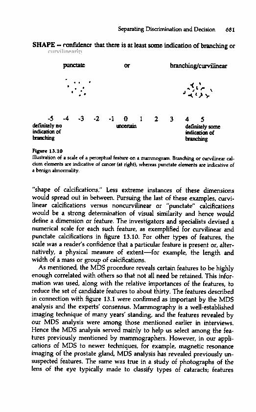
confidence

Figure 13.10Illustration of a scale of a perceptual feature on a mammogram. Branching or curvilinear calcium

elements are indicative of cancer (at right), whereas punctate elements are indicative ofa benign abnormality.

"shape of calcifications ." Less extreme instances of these dimensions

would spread out in between . Pursuing the last of these examples, curvi -linear calcifications versus noncurvilinear or "

punctate"

calcificationswould be a strong determination of visual similarity and hence woulddefine a dimension or feature. The investigators and specialists devised anumerical scale for each such feature, as exemplified for curvilinear andpunctate calcifications in figure 13.10. For other types of features, thescale was a reader' s confidence that a particular feature is present or, alternatively

, a physical measure of extent - for example, the length andwidth of a mass or group of calcifications .

As mentioned , the MDS procedure reveals certain features to be highlyenough correlated with others so that not all need be retained . This information

was used, along with the relative importances of the features, toreduce the set of candidate features to about thirty . The features describedin connection with figure 13.1 were confirmed as important by the MDSanalysis and the experts

' consensus. Mammography is a well -established

imaging technique of many years'

standing , and the features revealed byour MDS analysis were among those mentioned earlier in interviews .Hence the MDS analysis served mainly to help us select among the features

previously mentioned by mammographers . However , in our applications of MDS to newer techniques, for example, magnetic resonance

imaging of the prostate gland , MDS analysis has revealed previously unsuspected features. The same was true in a study of photographs of the

lens of the eye typically made to classify types of cataracts; features

Separating Disaimination and Decision 681

SHAPE - that there is at least some

punctate... ... .. .. .-s

definitely DOindicaboo oftnlx:hing

-4 -3 -2 -1 0~

1 2 3 4 Sdefinitely someindicatioo of~ g

indication of branching

bran c bin g/ curvilinear

0( ,~" t ,.. \J ~ C} ~

682 Swets

newly revealed by MDS analysis provided a more sensitive classification

than that previously available .

13 . 7 . 1 . 3 Determining the Final List of Features and Their Weights

We investigators believed that the set of thirty features that remained

after the consensus conference was too large to be workable and probably

contained several features that would not carry much weight in a diagnosis

, that is , would not be very predictive of malignancy . We therefore

made a second reading study and applied another statistical technique to

reduce the feature set to just the most important ones . We had in mind a

set of a dozen or so features . We wanted to know quantitatively how

predictive each of these features was so that we could assign a weight to

each , that is , a number reflecting its importance in diagnosis . We looked

ahead to a merging aid for the radiologist who , in reading mammograms ,

would assign a scale value to each feature , which would then be multi -

plied by the weight of that feature , such that the resulting products could

be linearly combined to calculate a probability of malignancy .

In the second reading study , the specialists applied the scales of the

thirty features that remained after the consensus conference to the images

of 100 new cases for which the diagnostic truth was known , including 50

cancers proven by biopsy and 50 noncancers established by one year of

follow -up . The statistical procedure of

"discriminant analysis

" was then

used to determine which minimal set of features was necessary and sufficient

to be retained in the final checklist , and to determine their relative

weights . This analysis shows specifically which features with which

weights serve to maximize discrimination acuity , where acuity is expressed

by a measure closely akin to the ROC area measure (Az ) defined earlier .

Twelve features were selected for the final set , to be used in creating a

checklist for radiologists . This final set of features included those with

high enough weights to contribute significantly , in our view , to discrimination

acuity and excluded those making only a minimal contribution .

13 . 7 . 1 . 4 The Merging Aid

The same discriminant analysis was the basis for the merging aid , the

computer program that linearly combined the twel~

e scale values given

to it by the radiologist for the twelve checklist features , appropriately

weighted , for each case read . The computer

's output , as mentioned , was

an estimate of the probability of cancer that radiologists could use in

making their own estimate . Readers might report a higher or lower probability

value for cases where they thought there was something in the

mammogram that was not captured adequately by the feature scales .

The concepts and details of how discriminant analysis determines a final

set of features for a checklist and then serves as a merging aid are the

subjects of entire books and manuals (e.g., Lachenbruch 1975), but I willattempt to capture briefly the intuitive essentials. Recall that the mammog-

raphy specialists gave a rating on each of thirty features (in a "master"

set) for each of 100 mammographic cases known to have cancer or not. Asimple way to determine which of the features are quantitatively the mostuseful in distinguishing cancer from noncancer cases would be to calculatefrom those ratings an ROC measure of acuity for each feature independently

. One problem with this approach is that there is no way to determine which of the thirty features constitute an appropriate smaller set.

Another problem with this approach is that there is no clear way tomerge a set of feature values into a single decision variable, namely, theprobability of cancer, especially because the features cannot be assumedto be independent. The form of discriminant analysis we used address esthese problems by implementing a stepwise feature selection procedure,in which features are selected in order of their acuity after taking theirintercorrelation into account. That is, the procedure first selects the mostdiscriminating feature and gives a measure of its diagnostic acuity, thenselects the feature that is second most discriminating, when only acuitybeyond that offered by the first is considered, and measures the additional(uncorrelated) acuity the second feature provides, and so on. This particular

second feature is not necessarily the one with the second highestacuity when features are considered independently. The procedure can beterminated when additional features are adding only insignificantly tototal diagnostic acuity. If you think of each mammogram as being represented

by a point in a multidimensional space (as in MDS analysis) thathas the final set of features (say, twelve) as dimensions, then the mam-

mograms indicating cancer collect in one cloudlike region of the spaceand those indicating no cancer collect in another. The discriminant analysis

determines the direction, or vector, through the space that best separates the two clouds. This determination serves to reduce the number of

dimensions of the space to just one dimension, namely, the line represented by the vector. The equation for that vector is a linear function of

the dimensions, and the coefficients of the equation represent the relativeweights of the features in diagnosis. The equation is called a "discriminantfunction."

This function constitutes the merging aid when individual mammogramcases are read. Scale values assigned by the reader to the features of agiven case are multiplied by their respective weights (the function's coefficients

) and added together to yield a discriminant score. In effect, themammogram being read is represented as a point along the discriminantvector. This point or score is then translated into a probability that themammogram at hand reflects the presence of cancer, and this probability


is the advisory estimate that is given as an aid to the mammogram reader(Getty et al. 1988).

13.7.1.5 Erperimental Test of the Effectiveness of the Aids

Six other radiologists, experienced but not specialized in mammog-

raphy, read a different set of cases (58 cancer, 60 noncancer) to provide anevaluation of the effectiveness of the two aids. They read the cases first intheir usual manner without the aids (

"standard condition") and then, after

six months, with them ("enhanced condition"

). In both instances, thereaders gave their degree of confidence, on a five-category scale, that acancer was present. The rating method described in section 13.3.1 wasused to construct an ROC for each reader in each condition. A groupROC for each condition was obtained by pooling the rating data of theindividual readers.

Figure 13.11 shows the ROCs for standard and enhanced conditions forthe group of six readers. The lower curve, for the standard reading, has anacuity measure (as defined in section 13.3.3) of Az = .81. The upper curve,for the enhanced reading, has an Az = .87. All six readers showed an

x =

Standard

a-

Enhanced

. 6 . 7 . 8 . 9 1 . 0

POSITIVE PROPORTION

3f\ lll

SO

d

3n ~ l

684 SwetsN

OU

~ OdO

~ d

1.0

.9

.8

.7

.6

.5

.4

.3

.2

.1

00 .1 .2 .3 .4 .5

FALSE


effect in the same direction, of about the same size; thus the finding ishighly unlikely to arise from chance or random variation.

As a control condition in the experiment, to help assure that theobserved difference was due to the aids, three of our readers reread thecases in the standard mode just before making the enhanced readings andthe other three reread the cases in the enhanced manner six months afterthe first enhanced reading. The Az values for rereadings in the standardmode were essentially the same as the Az values for the original standardreading, indicating that the passage of six months did not bring an increase

in Az. Likewise, the Az values in the first and second enhancedreadings were almost identical, indicating that the enhancement producedby the aids would be sustained over time. Incidentally, the aids broughtthe non specialist s

' performance up to that of the specialists. That improvement

may be even better than it looks, because our measure of thespecialists

' performance, while ostensibly in a standard condition, was

obtained after their experience in the interview, MDS study, and consensus conference, and we believe this measure is higher than it would be

had it been taken prior to that intensive experience.

13.7.1.6 Clinical Significance of the Observed Enhancement

More informative for purposes of this study than the overall acuity measures are the specific gains in TPP, reductions in FPP, or both that the aids

produced. Consider a decision criterion for recommending a biopsythat yields a point on the "standard" ROC at FPP = .20, TPP = .67, asindicated in figure 13.16 where the short dashed lines meet. It can beseen that for the same value of FPP = .20, the "enhanced" ROC showsTPP = .80- an improvement in TPP of .13, or an increase of 19 percent.Turning instead to the gain in acuity afforded by the aids as a reduction inFPP, it can be seen that for TPP = .67, the "enhanced" FPP = .08; thisvalue of .08 is .12 less than the "standard" FPP of .20 (a decrease of 60percent). The indication here is that, for 100 patients with cancer, the aidswill permit detection of cancers in about 13 additional patients (an increase

from 67 to 80); alternatively, for 100 patients without cancer, theywill permit avoidance of an unnecessary biopsy in about 12 additionalpatients (a decrease from 20 to 8). Other balances are possible in makinguse of the observed gain in acuity, for example, a simultaneous increase inTPP and decrease in FPP of approximately .06 each (a 9 percent increasein the TPP and a 30 percent decrease in the FPP).

Following this indication of the value of our feature-based approach tomammography, we have begun to design a computer-based tutorial program

for training new radiologists and for the continued education ofpracticing radiologists (Getty et al. 1992). We consider the possibility-

686 Swets

given that the perceptual feature approach does not depend on a knowledge of underlying anatomy and pathology- that paramedics can be

trained and assisted in reading mammograms with good acuity, a resultof especial value in areas or countries where radiologists are in shortsupply.

13.7.2 Optimizing the Decision Criterion

Choosing an appropriate decision criterion in almost any practical settingis difficult, and how to do so in mammography is by no means clear. Theaim of the next few paragraphs is to indicate that decomposing the discrimination

and decision process es is critical and that concepts of theoptimal criterion provide a structure for analyzing the problem and formoving toward a consensus.

13.7.2.1 The Expected Value Optimum

Can the expected value definition of the optimal decision criterion beapplied in this medical setting? As discussed in section 13.2.2.4, onewould need to estimate the prior probability of cancer in the populationof patients and to assign numerical benefits and costs to the four possiblediagnostic outcomes. Data are available on prior probabilities (called"prevalences

" in medicine) for two major populations, the populationinvolved in a screening program for women in general and the populationof patients who appear at a referral center because they have a high riskfor breast cancer or because a physical examination suggested the possibility

of a lump. The prior probability of cancer in screening populationsis about .02; in referral populations, about .32. This implies a sixteenfold difference in the optimal LR or slope measure 5 and, for any set ofbenefits and costs, would call for a large difference in the decision criterion

adopted in the two settings, with a far more lenient criterion beingappropriate for the referral setting. There have been several attempts,as discussed in the literature on medical decision making, to develop waysto assign benefits and costs to diagnostic outcomes (e.g., Weinstein andFineberg 1980). However, such an assignment is always very difficultwhen human lives are evaluated, and individual opinions may differwidely. One way to soften the demands of the expected value definitionis to quantify its overall ratio of benefits and costs without assigning allfour individual values: benefit (TP), cost (FP), benefit ( TN), and cost (FN).One could say, for example,

'1 would five times rather be right whencondition A exists (when cancer is present) than when condition B exists(when cancer is not present).

" Combining just that ratio with the ratio of

prior probabilities is enough to specify an optimal criterion.

13.7.2.2 The Optimal Criterion Defined by a Particular False PositiveProportion

Another way to bypass explicit benefits and costs is to select the criterionthat satisfies a specified limit on FPP. This definition of the criterion isused in testing statistical hypotheses, where the limit on FPP (the "type Ierror", or "level of significance

") is usually .05 (or .02 or .01). With this

criterion, benefits and costs are considered only tacitly in arriving at theproportion of false positive errors that can be tolerated. Anecdotally, thistolerable FPP is often thought to be around .10 in medical contexts.

13.7.2.3 Societal Factors in Setting a Criterion

The problem of choosing an appropriate decision criterion is illuminatedby looking directly at the values of FPP and TPP that are ~ttainable. Takethe top ROC in figure 13.5 as an approximation to the performance ofmammography (perhaps a little generous). The FPP = .10 just mentionedallows a TPP = .80. There is a strong desire in medical circles to increasethat TPP- to .90, say- because missing 2 of 10 patients with cancerseems like too many. But TPP = .90 brings along a FPP = .20. And a further

increase to TPP = .95 carries an increase to FPP = .35. Considerfurther those last two ROC operating points: TPP can be increased from.90 to .95 at a price of increasing FPP from .20 to .35. Consider them inconnection with a screening population, wherein, as I mentioned, about 2percent of the patients have a breast cancer. In a sample of 5,000 patients,100 will have cancer and 4,900 will not; hence, at the more lenient criterion

, 95 instead of 90 of the 100 cancers will be detected. Meanwhile, thenumber of unnecessary biopsies will increase by 735- from 4,900 xi

= 980 up to 4,900 x .35 = 1,715. Detecting 5 more cancers at a priceof 735 more unnecessary biopsies does not make the more lenient criterion

an obviously better balance of TPP and FPP than that of slightlystricter criterion. Choosing between those or any two criteria would seemto require some quantitative analysis of costs and benefits. Then again, thewishes of individual patients and their physicians may dominate, and bothpatients and physicians tend to read and interpret the odds very conservatively

. When physicians are asked to say how Iowa probability ofcancer will lead them to recommend biopsy, they indicate a range in theneighborhood of .05.

That the yield of biopsy is 20 to 30 percent in the United States suggests that the decision criterion is set with the desires of individual

patients and physicians in mind, rather than with a focus on what mightbe regarded as a cost-effective approach for society as a whole. England

'syield of about 50 percent reflects a notice ably stricter criterion, one possibly

more mindful of society's requirements. Societal strictures may be


688 Swets

effected by regulation or by the availability of services. As I observedearlier, if the U.S. population were to follow the national guidelines for

mammographic examinations, thus requiring exams in much larger numbers, and if the current criterion for biopsy were retained, there would

probably not be enough surgeons and pathologists available to supplythe resulting number of recommended biopsies. At that point, the issue of

choosing an appropriate decision criterion would take on a salience that isnot apparent now.

13.7.3 Adapting the Enhancements to Medical Practice

Now that we have a way to increase diagnostic acuity in mammographyand a way to think about the decision criterion for recommending treatment

, how might these results be put into practice? In a project just underway, my colleagues and I are working on a computer system that will

embed these enhancements in a network of several related work stations. Iam pleased to say that the radiologists with whom we work have beenvery cooperative. Some may regret systematization at the expense of artin reading images, but radiologists are scientifically and quantitativelyminded and most can be expected to adopt a system that provides ademonstrated gain in acuity.

Another benefit that derives &om the present approach is a stan-dardization of radiologists

' reports to referring clinicians and surgeons.

There is now a good deal of clamor nationally among associations representing the recipients of those reports, and several government agencies

have worked with the American College of Radiology to bring about astandardized vocabulary for the prose reports. In the system we are

building, the radiologist's key presses (or spoken words) to indicate scale

values to the computer will be converted automatically to corresponding,appropriate sentences in the report (Swets et al. 1995). In fact, the perceptual

features as named in the study described above are the elements of astandard vocabulary or lexicon currently espoused by the American College

of Radiology (Kopans and D'Orsi 1992).

Though no data exist, I believe that standardizing perception in mam-

mography (the scaling of features) will give better results than standard-

izing language alone. The time saved for the radiologist by automatic

report generation may compensate effectively for whatever additionaltime is required by explicitly scaling perceptual features in reading an

image. Moreover, the reports can be delivered to their intended recipientsas they are generated. Reports can also be stored in a database, along with

subsequent outcome data, which may afford several benefits. Individual

radiologists can be assisted to greater acuity by tutorials tailored to the

knowledge they need, for example, how better to scale particular features.

A database can also assist in standardizing decision criteria across theradiologists in a given hospital, say, by reporting the yields of biopsiesthey recommend. On another tack, digital imagery will permit radiologiststo secure second opinions &om anywhere, in feature-by-feature detail, andto resolve differences of opinion by reference to quantitatively scaledfeatures. Finally, there is a possibility that the use of a standard, approvedprocedure will reduce a practitioner

's liability in suits for malpractice.The next section briefly describes another possible application to the

interpretation of diagnostic images. But note that images are not essential to this approach. Neither, for that matter, is a two-alternative response.

One might, for example, develop features related to a psychiatric patient- the patient

's nonadaptive behavior, risk level for dangerous behaviorsor chemical dependencies, social resources, and so on- and, in turn,develop a system that combines ratings of those features to enable achoice among several graded treatment possibilities, ranging across standard

outpatient treatment, more &equent visits, and acute inpatient care.

13.8 Detecting Cracks in Airplane Wings: A Second PracticalExample

The possibilities for improving discrimination acuity and adopting an

appropriate decision criterion , as demonstrated for mammography , existin similar diagnostic fields. Consider an example &om materials testing ,wherein the imaging techniques of ultrasound and eddy current are usedto visualize flaws in metal structures . The specific example is the detectionof cracks in airplane wings by maintenance personnel . Incidentally , a

diagnostic extension of this simple detection task that involves recognition as well requires a characterization of the severity of a flaw in order

to project the time course of its developing into something still moreserIous.

13.8.1 Discrimination Acuity and the Decision Criterion

There is clearly a lot at stake here: a false negative decision can lead to acatastrophic accident and dramatic loss of lives. Still, a false positive decision

takes a plane out of service unnecessarily at substantial costs in dollarsand convenience. On balance, as in mammography, the costs and benefitsseem to suggest a lenient criterion for declaring a flaw. On the otherhand, the prior probability of a dangerous flaw, although increasing withan aging fleet of airplanes, is still very low, and low prior probabilities,even with moderate criteria, tend to produce a large number of false positives

, possibly so large as to be unworkable. Thus attention to both discrimination acuity and the decision criterion is required.


13.8.2 Positive Predictive Value

The idea that airplane fleet operators cannot just proceed with a lenientdecision criterion, accepting many false positives in order to reduce false

negatives to near zero, may need support. An important concept in thisconnection and many others is the predictive value of a positive decision.The positive predictive value (PPV) is the proportion of positive responsesthat are true. In the two-by-two array of table 13.2, it is defined asaf(a + b); that is, it is a TP proportion based on the occurrence of the response

(row sum), rather than the TPP based on the occurrence of thestimulus (column sum) that I have emphasized thus far. It is also referredto as the "inverse TP proportion,

" because it goes backward from response to stimulus. Note that I introduced this concept in speaking of the

yield of the biopsy procedure in the mammography study. The point isthat low prior probabilities and lenient decision criteria conspire to produce

a low PPV, such that the observer's decisions often "cry wolf " whenthere is no wolf .

I have looked at the values of PPV that can be expected in another aircraft

setting, where specialized sensors (detectors) give in-flight warningsto pilots about various imminent dangers- including collision, enginefailure, ground proximity , and wind shear. Even when it is assumed thatthe detectors are extremely acute and the decision criteria are very strict,the PPV can easily be lower than .05, so that only 1 in 20 warnings isvalid (Getty et al. 1995). Such a low predictive value can be inappropriate,for example, in a setting in which a simple

"fly-around" by a plane in final

approach to a major airport- a fly-around in response to a wind shear

warning, say- can put air traffic control under additional strain for several hours, and thus endanger many other aircraft in addition to the one

taking the first evasive action. In short, the cost of a false positive decisionis not negligible. In fact, pilots come to ignore warnings from unreliable

systems when they have other important things to do.An example from medical diagnosis of the effect of low prior proba-

bilities on PPV comes from testing for the human immunodeficiency virus(HIV) of AIDS. For low risk populations- for example, blood donors or a

company's employees- the prior probability of HIV is about .003 (Bloom

and Glied 1991). Ordinarily , in such a setting, a positive outcome on a

typical screening test is followed by a more conclusive (and expensive)confirmatory test (Schwartz, Dans, and Kinosian 1988). Using the Collegeof American Pathologist

's estimates of test performance (TPP and FPP) forthe best screening and confirmatory tests (Bloom and Glied 1991), I calculate

that after a positive result on both tests, the PPV is .13. Hence, 6 of7 individuals diagnosed as positive in this manner are told they have theHIV when they do not in fact have the HIV (Swets 1992). As another

690 Swets

example, the issue of Newsweek magazine that appeared as I write (19 April ,1994) mentions a study in which 65 exploratory surgeries for ovariancancer were performed for every cancer found by the surgery- to manyof us, no doubt, an incredibly low yield for a risky surgical procedure. Theprior probability (lifetime risk) of ovarian cancer was said to be .015; evenfor the category of patients at special risk for ovarian cancer because thatdisease has occurred in the family, the prior probability is only .05.

13.8.3 Data on the State of the Art in Materials Testing

The U.S. Air Force kindly gave me access to the data &om its major studyof detecting cracks in airplane wings. In the study, 148 metal specimenswith and without flaws were carried to 17 air force bases, where theywere inspected, in total, by 121 technicians using ultrasound imaging and133 technicians using an eddy current imaging technique.

The performance of each technician in this study is depicted by a pointon an ROC graph in figures 13.12 and 13.13. The impact of just a glanceat these graphs is the main result: the variation across technicians is about

Separating Discrimination and Decision 691N

OIJ

. YO

dOY

d

3AIJ

. I SO

d

3nyJ

.

Figure 13.12Relative operating characteristic (ROO data points for 121 technidans inspecting metalspeamens for cracks with an ultrasound technique.

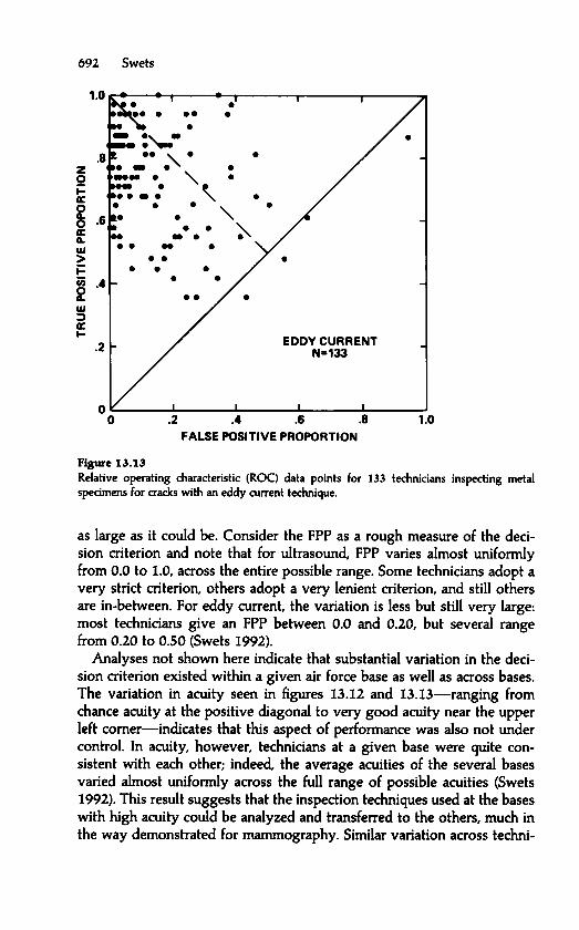
1 . 0

. .

.

. 8

.

.

.

. 6

.

.

. .

. 4

. .

. .

2

EDDY CURRENT

.

N

=

133

0

0 . 2 . 4 . 6 . 8 1 . 0


-Relative operating characteristic (ROq data points for 133 technicians inspecting metalspecimens for cracks with an eddy current technique.

as large as it could be. Consider the FPP as a rough measure of the decision criterion and note that for ultrasound , FPP varies almost uniformly

from 0.0 to 1.0, across the entire possible range. Some technicians adopt a

very strict criterion , others adopt a very lenient criterion , and still othersare in-between . For eddy current , the variation is less but still very large:most technicians give an FPP between 0.0 and 0.20, but several rangefrom 0.20 to 0.50 (Swets 1992).

Analyses not shown here indicate that substantial variation in the decision criterion existed within a given air force base as well as across bases.

The variation in acuity seen in figures 13.12 and 13.13- ranging fromchance acuity at the positive diagonal to very good acuity near the upperleft comer - indicates that this aspect of performance was also not undercontrol . In acuity , however , technicians at a given base were quite consistent

with each other ; indeed, the average acuities of the several basesvaried almost uniformly across the full range of possible acuities (Swets1992). This result suggests that the inspection techniques used at the baseswith high acuity could be analyzed and transferred to the others , much inthe way demonstrated for mammography . Similar variation across techni -

692 SwetsN

OI

. 1 Y

Od

O

Yd

3AI

. 1IS

Od

3ny

. 1

Fiaure 13.13

clans in acuity has been found in other studies of materials testing , for

example, in the examination by eddy current of steam generators in powerplants (Harris 1991).

13.8.4 Diffusion of the Concept of Decomposing Diagnostic Tasks

As a counter to the example of medical radiology, where the ROC hasbeen used extensively, it should be noted that the ROC approach has notbeen picked up in the materials-testing field. Over ten years, I carried the

message along with the data of figures 13.12 and 13.13 to the Air Forceand the Army, and also to the Federal Aviation Administration and a majorcommercial aircraft manufacturer, and further to the research laboratory ofthe U.S. electric power companies, to no avail. I am told that a tutorialarticle in the field's professional magazine (Swets 1983) has begunrecently to have some impact ( W. S. Brown, personal. communication,December, 1995), but I have not been able to obtain the reports.

There are also blind spots within clinical medicine. For example, theseveral tests for screening for the HIV of AIDS have widely differentacuities and decision criteria (Swets 1992). Moreover, each test's decisioncriterion is held constant across different settings, for example, whetherused on donated blood or to diagnose individuals- two applications inwhich the cost of a false positive decision differs consider ably. Further,those criteria remain fixed when screening different populations of individuals

for which the prior probability differs greatly, say, from .003 (low-risk blood donors) to .45 (methadone clinic attendees).

However, again on the brighter side, the idea of using an ROC measureof acuity is making noticeable progress in weather forecasting, where itis overcoming resistance from advocates historically of other measures(Williams 1985; Brunet, Verret, and Yacowar 1987; Sarrazin and Wilson1987). The ROC is generally accepted by evaluators in the field of information

retrieval (Brookes 1968; Heine 1973). A laboratory of the NationalAeronautics and Space Administration is now examining the applicationof signal detection theory and the ROC to in-flight warning systems(Getty et al. 1995). If I have any idea about the unevenness in the acceptance

of the decomposition concepts, it is a matter of the size of the diagnostic problem, and perhaps the scientific versus technological bent of the

people involved. University radiologists, laboratory meteorologists, andinformation retrieval methodologists do studies and write articles, andhave the frame and peace of mind to want to do them right . Managingthe nation's aircraft travel, power plants, and disease epidemics no doubtattracts individuals having a different frame of mind and gives them no

peace of mind. It is all the more a shame, but we can easily imagine thattechnical matters that seem difficult or esoteric get blown off desks at the


Federal Aviation Administration, the Department ofand Drug Administration (Swets 1991b).

13.9 Some History

For a century in psychology, beginning with the systematic study of sensory detection and recognition around 1850 (Fechner 1860), the dominant psychological position was that the two process es of discrimination

and decision were essentially one- that the discrimination process ledautomatically to response A or response B. Decisions themselves werethought not to be involved; rather, the discrimination process includedan automatic threshold device that detennined response A or response Bdepending on whether a particular, fixed strength of evidence was exceeded

or not, with the particular strength being detennined by the phys-

iological makeup of the organism. There was for some psychologists aconcern that attitude could affect the observer's responses, but in general,it was thought that discrimination acuity could be measured without concern

that the measures would be distorted or made unreliable by variationin a separate decision process.

The decomposition of discrimination and decision into two measurableprocess es was suggested and made possible about 1950 by a generaltheory of signal detection. The theory was developed by engineersWesley Peterson and Theodore Birdsall for theoretical devices- called"ideal observers"- in the context of radar (Peterson, Birdsall, and Fox1954). The discrimination problem they addressed was to determinewhich values of certain physical measurements of electronic wavefonnsindicated the presence of a signal that represents, for example, theapproach of an enemy plane. The generality of signal detection theory isindicated by the similarity of this discrimination problem and that ofmammography.

The decision part of signal detection theory was derived from statisticaldecision theory ( Wald 1950), which is an extension of the theory of testing

statistical hypotheses developed by Jerzy Neyman and Egon S. Pear-son in 1933. The earlier one-process view of detection and recognition inpsychology mirrored statistical hypothesis testing in the fonn popularizedby R. A . Fisher at about the same time (Gigerenzer and Murray 1987). Indetennining, for example, whether the mean of population A differs fromthe mean of population B, a fixed decision criterion is assumed, akin to afixed threshold, such that the probability of deciding A ~ B when in factA = B (a "type I error") is no greater than .05 (or .02 or .01). In thebroader decision theory, the placement of a variable decision criterion inany instance depends on the prior probabilities of A ~ B and A = B and

694 Swets

Energy , and the Food

on the benefits and costs of correctly and incorrectly deciding that A #= Bor that A = B. The use of Fisher's fixed criterion in statistical analysis(with prior probabilities and benefits and costs being only tacit) is common

when making an inference from data, that is, a "knowledge claim." Avariable criterion (with those situational variables being explicit) is moreappropriate when, instead, some action is to be taken.

Psychologist Wilson P. Tanner, Jr., and I (1954), working with thesignal detection theorists, proceeded to show that human observers insimple sensory detection tasks (detecting brief tones or spots of light)base their responses on a variable decision criterion that takes into account

the prior probability that a "signal" is present and the benefits and

costs associated with the various possible decision outcomes. Althoughthe human observers did not match exactly the optimal expected valuecriterion, their criteria under different conditions of prior probabilities andbenefits and costs were highly correlated with the optimum. In general,the empirical ROCs obtained from these observers looked like the theoretical

curves shown in earlier sections (Swets, Tanner, and Birdsall 1961).This inclusion of nonsensory factors in the theory of simple sensory

tasks- "expectancy

" and "motivation" in psychological terms- was nodoubt part of the spirit of the times as cognitive psychology came intoview. Gird Gigerenzer and Richard Murray (1987) have recently developedin some detail how perceptual and cognitive theory have followed statistical

theory, how the human has been viewed as an intuitive statistician.In the human sensory experiments first following on signal detectiontheory, the decision criterion was actually manipulated by varying priorprobabilities of the stimuli and benefits and costs of the stimulus-responseoutcomes. Without overt manipula Hon, you might suspect that decisioncriteria would vary from one observer to another based on individualimpressions of implicit prior probabili Hes and implicit benefits and costs.For example, one observer might want to demonstrate acuity by maxi-

mizing the true positive proportion, while another might want insteadnot to issue a false positive response, perhaps because it might be viewedas an hallucination. Distinguishing such different tendencies by isolatingdecision effects is necessary if acuity is to be measured validly (Swets1961; 1973; 1988).

James Egan (1958) soon extended the psychological coverage of signaldetection theory to recognition memory, that is, to deciding whether anitem presented (a word, say) was on a list shown earlier. Other psychologists

then applied the theory to attention, imagery, reaction time, manualcontrol, learning, conceptual judgment, personality, and animal behavior(Swets 1973). The first extension to a practical diagnostic problem was toinformation retrieval, where one wishes to single out those documents ina library that satisfy a par Hcular need for information and to avoid the


irrelevant documents (Swets 1963). Lee Lusted (1968) showed the valueof the theory

's decomposition of diagnostic tasks in radiology, presaginghundreds of published applications in clinical medicine.

Some aspects of signal detection theory, without the variable decisioncriterion and ROC, were present in earlier psychological theory. For

example, in the 1920s, the innovative psychometrician Louis Leon Thur-stone (1927a,b) proposed stimulus distributions such as those in figure 13.2as part of an extensive statistical theory of discrimination, calling them"discriminal process es." For Thurstone, however, the two stimuli werenot polarized as positive and negative, and the (response) criterion wasviewed in the theory as being fixed at the symmetrical location, where thetwo curves cross. Hence his theory did not go on to separate decision anddiscrimination process es.

The ROC was developed in signal detection theory, where it is calledthe "receiver operating characteristic,

" and is a unique contribution of thattheory. I alert you to the tendency of statisticians to remark that the ROCis "essentially the power curoe of statistics." Rather, the power curve is theS-shaped curve of TPP plotted against the difference between the meansof two statistical hypotheses for a fixed, low value of FPP (e.g., .05). Thus,although the power curve includes the same three variables as the ROC,it shows how acuity and TPP vary together for a single FPP. It does notshow the interplay of TPP and FPP for each level of acuity, that is, a variable

decision criterion, and thus gives no insight into the separationof discrimination and decision process es. Indeed, what is essentially the

power curve appears also in signal detection theory, where it is called the"betting curve,

" and it has thrived for over a century in psychology,where it is called the "psychometric function,

" without suggesting the

impact of the ROC (Green and Swets 1966).Finally, a few comments on method and terminology, to help the reader

who may see the ideas of the chapter in psychological contexts. In earlysections of this chapter, I mentioned three data collection methods, whichI called the "

yes-no," "

rating," and "

paired-comparison" methods. In

sensory psychology, where the incentive is to minimize criterion effectsin the simplest way, the frequently used paired-comparison method iscalled the "two-alternative forced-choice" (2AFC) method. In connectionwith the other two methods, both used to determine an ROC, I used the

general terms true positive and false positive proportions. In psychology,where the legacy of signal detection theory is most familiar, these tendto be called, respectively,

"hit " and "false alarm proportions." The threemethods existed long before signal detection theory (SOT) was developed

, but tended to give different results. SOT related the three methods

quantitatively and rationalized them by showing theoretically that theygive, under fixed conditions, the same value of a common measure of dis-

696 Swets


crimination acuity (Swets, Tanner, and Birdsall 1961). Empirical demonstrations of the validity of this theoretical prediction were important in

establishing the general validity of the concepts of signal detectiontheory .

Suggestions for Further ReadingThree textbooks on signal detection theory and ROC analysis are those of Green and Swets(1966), Egan (1975), and Maanillan and Creelman (1991). A collection of articles treats therange of subjects of this chapter (Swets 1996). A pair of articles shows representative ROCs&om several psychological and diagnostic tasks and develops the implications of their fonnfor alternative measures of discrimination acuity (Swets 1986a,b).

The examples given here of experimental decomposition of discrimination and decisionprocess es are treated further as follows: vigilance (Davies and Parasuraman 1982; See et al.1995); recognition memory (Murdock 1974); polygraph lie detection (Shakhar, Lieblich, andKugelmass 1970; Swets 1988); infonnation retrieval (Swets 1963, 1969); and weather forecasting

(Swets 1986b, 1988).On combining observations to achieve greater acuity, see Green and Swets (1988), Metz

and Shen (1992), Seltzer et al. (1992), and Swets (1984). Articles describing the enhancementof accuracy of mammography are by Getty et al. (1988), Swets et al. (1991), and D'Orsi et al.(1992). A textbook treatment of evaluation methods in diagnostics is given by Swets andPickett (1982). Measures of diagnostic acuity in several settings are given by Swets (1988);choosing the best decision criterion in diagnostics is discussed by Swets (1992).

For the background and history of signal detection theory in engineering, statistics, andpsychology, see Swets (1973, 1996) and Gigerenzer and Murray (1987).

Problems

13.1 Figure 13.2 shows probability distributions corresponding to stimuli A and B, respec-

tively , and a decision criterion Xc at the midpoint (mean) of the A distribution. The likelihoodratio of this criterion is 2.5. The value of TPP resulting from the criterion is .50; the value ofFPP is .15; as represented by hatched and crosshatched areas. What would TPP, FPP, and LRcbe for a criterion at the midpoint of the B distribution?13.2 The table below presents illustrative rating scale data. Plot the relative operatingcharacteristic (ROC) for these data. Estimate by a graphical method the slope measure 5 ofthe decision criterion for each data point.

Stimulus

Abnormal Normal

Response (positive) (negative)

I . very likely abnormal 350 252. probably abnormal 50 503, possibly abnormal 40 754. probably normal 35 ISO5. very likely normal 25 200

13.3 What are the expected payoffs (average over many decisions) of the diagnostic systems performing as in table 13.3 (system A), table 13.4 (system B) and table 13.5 (system C).

if the benefits and costs are TP = 10. FP = - 8, FN = - 4, and TN = 2? What is the optimallikelihood ratio criterion. LRc. for each system?

13.4 Suppose that the ROCs of figure 13.6 give the acuities of three weather-forecastingsystems for predicting frost that are available to a fruit grower whose produce is susceptibleto damage by frost. System A (Az = .75) is the daily newspaper; system B (Az = .85) is theNational Weather Service's prediction given by telephone; and system C (Az = .95) is acommercial service that focuses on frost and precise local areas. Suppose further that theoptimal decision criterion for a particular grower is LR, = 1.0. How would you express thegains in forecast accuracy that may be achieved in moving from system A to B to a13.5 Suppose that the data in tables 13.3, 13.4, and 13.5 were obtained in an evaluation ofthree alternative detection systems designed to warn a pilot of the possibility of midair collision

with another aircraft. The frequencies in the rows give the numbers of warnings issuedby the systems (positive response) and not issued (negative response) when the present condition

was truly dangerous (left column) or not truly dangerous (right column).Call the three systems A (table 13.3), B (table 13.4), and C (table 13.5). Which system

would you choose if you were required to put one of them into routine operation7 What isthe "positive predictive value" for each system that is implied by the data; that is, after alarge number of warnings by each, what proportion of warnings would have truly signified adangerous condition7

References

Ackerman. L. V.. and Gose. E. E. (1972) Breast lesion classification by computer and Xero-

radiograph. Cancer 30 (4). 1025- 1035.Banks. W. P. (1969). Criterion change and response competition in unlearning. Journal of

Erperimental Psychology 82. 216- 223.Barr-Brown. M.. and White. M. J. (1971). Sex differences in recognition memory. Psychonomic

Science 25. 75- 76.Bloom. D. E.. and Glied. S. (1991). Benefits and costs of HIV testing. Science 252. 1798- 1804.Broadbent. D. G. (1971). Dedsion and stress. London: Academic Press.Broadbent. D. G. and Gregory. M. (1963). Vigilance considered as a statistical decision. British

Journal of Psychology 54. 309- 323.Brookes. B. C. (1968). The measures of information retrieval effectiveness proposed by

Swets. Journal of Documentation 24. 41- 54.Brunet. N.. Verret. R.. and Yacowar. N. (1987). Comparison of MOS and perfect PROG

systems in producing numerical weather element forecasts. Tenth Conference onProbability and Statistics in Atmospheric Sciences. Edmonton. Canada. Boston. MA:American Meteorological Society. 12- 17.

Buckner. D. N.. and McGrath. J. J. (Eds.) 1963. Vigilance: A symposium. New York: McGraw-Hill.

Da Polito. F.. Barker. D.. and Wiant. J. (1971). Context in semantic information retrieval.Psychonomic Science 24. 180- 182.

Davies. D. R.. and Parasuraman. R. (1982). The psychology of vigilance. New York: AcademicPress.

Davies. R. M.. and Corrigan. B. (1974). Linear models in decision making. Psychological Bulletin81. 95- 106.

Donald son. W.. and Murdock. B. B.. Jr. (1968). Criterion change in continuous recognitionmemory. Journal of Erperimental Psychology 76. 325- 330.

D'Orsi, C. J.. Getty. D. J., Swets. J. A.. Pickett. R. M.. SeltzerS. E.. and McNeil. B. J. (1992).Reading and decision aids for improved accuracy and standardization of mammo-

graphic diagnosis. Radiology 184. 619- 622.Egan. J. P. (1958). Recognition memory and the operating characteristic. Technical Note AFCRC-

TN-58-51. Indiana University. Hearing and Communication Laboratory. See Green.

698 Swets


D. M., and Swets, J. A. (1966/1988). Signal detection theory and psychophysics. NewYork: Wiley.

Egan, J. P. (1975). Signal detection theory and ROC analysis. New York: Academic Press.Egan, J. P., Greenberg. G. Z., and Schulman. A. I. (1961). Operating characteristics, signal

detectability, and the method of free response. Journal of the Acoustical Society ofAmerica 33, 993- 1007.

Frankmann, J. P., and Adams, J. A. (1962). Theories of vigilance. Psychological Bulletin 59,257- 272.

Fechner, G. T. (1860). Elemente der Psychophysik. Leipzig. Germany: Breitkopf and Hartel.English translation of Volume 1 by HE . Adler, D. H. Howes, and E. G. Boring (Eds.),Elements of Psychophysics. New York: Holt, Rinehart, and Winston, 1960.

Gale, A. G., Roebuck. E. J., Riley, P., and Worthington, BS . (1987). Computer aids tomammographic diagnosis. The British Journal of Radiology 60, 887- 891.

Getty, D. J., Pickett, R. M., D'Orsi, C. J., Freeman. B. F., and Swets, J. A. (1992). Computerassisted instruction in radiology. Bolt Beranek and Newman Inc., Final report underNIH Grant No. 5 R01 CA45574-03.

Getty, D. J., Pickett, R. M., D'Orsi, C. J., and Swets, J. A (1988). Enhanced interpretation ofdiagnostic images. Investigative Radiology 23(4), 240- 252.

Getty, D. J., Swets, J. A., Pickett, R. M., and Gonthier, D. (1995). System operator responseto warnings of danger: A laboratory investigation of the effects of the predictivevalue of a warning on human response time. Journal of Experimental Psychology:Applied 1(1), 19- 33.

Gigerenzer, G., and MurrayD . J. (1987). Cognition as intuitive statistics. Hi Usdale, NJ: Erlbaum.Green, D. M., and Swets, J. A. (1966). Signal detection theory and psychophysics. New York:

Wiley. Reprint (with updated topical bibliography), Los Altos Hills, CA: Peninsula,1988.

Hammond, K. R., Harvey, L. 0 ., Jr., and HastieR. (1992). Making better use of scientificknowledge: Separating truth from justice. Psychological Science 3, 80- 87.

HarrisD. H. (1991). Eddy currents steam generator data analysis performance. Paper presented at the American Society of Mechanical Engineers International Joint Power

Generation Conference. San Diego, CAHeine, M. H. (1973). The inverse relationship of precision and recaU in terms of the Swets

model. Journal of Documentation 29, 81- 84.Kopans, D., and D'Orsi, C. J. (1992). ACR system enhances mammography reporting.

Diagnostic Imaging, September, 125- 132.Lachenbruch P. (1975). Discriminant analysis. New York: Hafner.Lusted, L. (1968). Introduction to medical decision making. Spring field, IL: Thomas.Macmillan, N. A., and Creelman, C. D. (1991). Detection theory: A user's guide. New York:

Cambridge University Press.Mackle, R. R. (Ed.) 1977. Vigilance: Relationships among theory, operational perfonnance, and

physiological correlates. New York: Plenum.Mackworth, N. H (1950). Research on the measurement of human performance. Medical Research

Council Special Report Series No. 268. London: His Majesty's Stationery Office.

Mandler, G., Pearlstone, Z., and Koopmans, H. S. (1969). Effects of organization and semanticsimilarity on recall and recognition. Journal of Verbal Learning and Verbal Behavior 8,410- 423.

Mason, I. (1982a). A model for assessment of weather forecasts. Australian MeteorologicalMagazine 37, 75- 81.

Mason, I. (1982b). On scores for yes/no forecasts. Ninth Conference on Weather Forecastingand Analysis, Seattle, W A Boston, MA: The American Meteorological Society, 169-174.

McNichol. D.. and Ryder. L. A. (1971). Sensitivity and response bias effects in the learning offamiliar and unfamiliar associations by rote or with mnemonic. Journal of ExperimentalPsychology 90. 81- 89.

Metz. C. E.. and Shen. J-H. (1992). Gains in accuracy from replicated readings of diagnosticimages: Prediction and assessment in terms of ROC analysis. Medical Decision Making12. 60- 75.

Miller . E.. and Lewis. P. (1977). Recognition memory in elderly patients with depression anddementia: A signal detection analysis. Journal of Abnonnal Psychology 86(1). 84- 86.

Murdock. B. B.. Jr.. (1968). Serial order effects in short-term memory. Journal of ExperimentalPsychology. Monograph Supplement 76. 1- 15.

Murdock. B. B.. Jr. (1974). Human memory: Theory and data. Hillsdale. NJ: Erlbaum.Murdock B. B.. Jr.. and Duffy. P. O. (1972). Strength theory and recognition memory. Journal

of Experimental Psychology 94(3). 284- 290.Neyman. J.. and Pearson. ES . (1933). On the problem of the most efficient tests of statistical

hypotheses. Philosophical Transactions of the Royal Society of London. Series A. 289- 337.Parasuraman. R.. and Davies. DR . (1977). A taxonomic analysis of vigilance performance. In

R. R. Mackle (Ed.). Vigilance: Relationships among theory. operational per/onnance, andphysiological co" elates. 559- 574. New York: Plenum.

Peterson. W. W.. Birsdsall. T. G.. and Fox. W. C. (1954). The theory of signal detectability.Transactions of the IRE Professional Group on Infonnation Theory PGIT-4. 171- 212.Reprinted by R. D. Luce. R. R. Bush. and E. Galanter (Eds.). Readings in mathematicalpsychology. 167- 211. New York: Wiley. 1963.

Raser. G. (1970). Meaningfulness and signal detection theory in immediate paired-associaterecognition. Journal of Experimental Psychology 84. 173- 175.

Ries. L. A. G.. Miller . B. A.. Hankey. B. F.. et al. (1994). Cancer statistics review 1973- 91:Tables and graphics. NIH Publication No. 94-2789. National Cancer Institute.

Sarrazin. R.. and Wilson. L. J. (1987). Comparison of MOS and perfect PROG probability ofprecipitation forecasts using the signal detection theory model. Tenth Conference onProbability and Statistics in the Atmospheric Sciences. Edmonton. Canada. Boston.MA : American Meteorological Society. 95- 100.

Saxe. L.. Dougherty. D.. and Cross. T. (1985). The validity of polygraph testing. AmericanPsychologist 40(3). 355- 366.

Schwartz. J. S.. Dans. P. E.. and Kinosian, B. P. (1988). Human immunodeficiency virus testevaluation. performance. and use: Proposals to make good tests better. Journal of theAmerican Medical Association 259. 2574- 2579.

See. J. E.. Howe. S. R.. Warm. J. S.. and Dember. W. N. (1995). A metaanalysis of thesensitivity decrement in vigilance. Psychological Bulletin 117(2). 230- 249.

SeltzerS . E.. Getty D. J.. Tempany. C. M . C.. Pickett. R. M .. Schnall. M . D.. McNeil. B. J..and Swets. J. A . (1997). Staging prostate cancer with MR imaging: A combinedradiologist-computer system. Radiology 202. 219- 226.

SeltzerS. E.. McNeil , B. J.. D'Orsi. C. J.. Getty. D. J.. Pickett. R. M .. and Swets. J. A. (1992).

Combining evidence from multiple imaging modalities: A feature-analysis method.Computerized Medical Imaging and Graphics 16(6). 373- 380.

Shakhar. C. B.. Lieblich. I.. and Kugelmass. S. (1970). Guilty -knowledge technique: Application of signal detection measures. Journal of Applied Psychology 54(5). 409- 413.

Shepard. R. N. (1964). Attention and the metric structure of the stimulus space. Journal ofMathematical Psychology 1. 54- 87.

Shiffman. S. S.. Reynolds. M . L.. and Young. F. W. (1981). Introduction to multidimensionalscaling. New York: Academic Press.

Sickles. E. A .. Ominsky. S. A . Sollitto. R. A .. et al. (1990). Medical audit of a rapid throughput mammography screening practice: Methodology and results of 27.114 examinations. Radiology 175. 323- 327.

700 Swets

Swets, J. A. (1961). Is there a sensory threshold7 Science 134 (3473). 168- 177.Swets. J. A. (1963). Information retrieval systems. Science 141 (3577). 245- 250.Swets. J. A. (1969). Effectiveness of information retrieval methods. American Documentation

20. 72- 89. Reprinted in B. Griffith (Ed.), Key papers in information science. 349- 366.White Plains, NY: Knowledge Industry, 1980.

Swets. J. A. (1973). The relative operating characteristic in psychology. Science 182 (4116).990- 1000.

Swets, J. A. (1977). Signal detection theory applied to vigilance. In R. R. Mackle (Ed.).Vigilance: Relationships among theory, operational performance. and physiological co" elates.705- 718. New York: Plenum.

Swets, J. A. (1983). Assessment of NDT Systems: I. The relationship of true and false detections; II. Indices of performance. Materials Evaluation 41. 1294- 1303.

Swets. J. A. (1984). Mathematical models of attention. In R. Parasuraman and R. Davies(Eds.), Varieties of attention. 183- 242. New York: Academic Press.

Swets. J. A. (1986a). Indices of discrimination or diagnostic accuracy: Their ROCs and

implied models. Psychological Bulletin 99(1), 100- 117.Swets, J. A. (1986b). Form of empirical ROCs in discrimination and diagnostic tasks: Implications

for theory and measurement of performance. Psychological Bulletin 99(2). 181-

198.Swets. J. A. (1988). Measuring the accuracy of diagnostic systems. Science 240(4857). 1285-

1293.Swets, J. A. (1991a). Normative decision making. In J. Baron and R. V. Brown (Eds.), Teaching

decision making to adolescents. 273-':'296. Hillsdale. NJ: Erlbaum.Swets. J. A. (1991b). The science of high-stakes decision making in an uncertain world.

Science and Public Policy Seminar of the Federation of Behavioral. Psychological. andCognitive Sciences, Rayburn House Office Building. WashingtonD.C.. September 6.

Swets. J. A. (1992). The science of choosing the right decision threshold in high-stakes

diagnostics. American Psychologist 47(4). 522- 532.Swets. J. A. (1996). Signal detection theory and ROC analysis in psychology and diagnostics.

Mahwah. NJ: Erlbaum.Swets. J. A.. Getty. D. J.. Pickett. R. M.. D'Orsi. C. J.. SeltzerS. E., and McNeil. B. J. (1991).

Enhancing and evaluating diagnostic accuracy. Medical Decision Making 11(1). 9- 18.Swets, J. A.. Getty. D. J.. Pickett. R. M.. SeltzerS. E.. D'Orsi. C. J.. Frenna. T.. Freeman. B. F..

Mateer. M.. and Hermann. L. (1995). Increasing the accuracy of mammogram interpretation. Bolt Beranek and Newman Inc.. Annual report to U.S. Army Medical

Research and Materiel Command. Contract No. DAMO17-94-C-4082.Swets. J. A.. and Pickett. R. M. (1982). Evaluation of diagnostic systems: Methods from signal

detection theory. New York: Academic Press.Swets, J. A.. Tanner. W. P.. Jr.. and Birdsall. T. G. (1961). Decision process es in perception.

Psychological Review 68. 301":'340.Szucko. J. J.. and Kleinrnuntz. B. (1981). Statistical versus clinical lie detection. American

Psychologist 36(5). 488- 496.Thurstone. L. L. (1927a). A law of comparative judgment. Psychological Review 34. 273- 286.Thurstone. L. L. (1927b). Psychophysical analysis. American Journal of Psychology 38. 368-

389.Tanner. W. P.. Jr.. and Swets. J. A. (1954). A decision-making theory of visual detection.

Psychological Review 61. 401- 409.Waldo A. (1950). Statistical decision functions. New York: Wiley.Weinstein. M. C.. and Fineberg. H. V. (1980). Clinical decision analysis. Philadelphia. PA:

Saunders.


702 Swets

John A . Swets is Chief Scientist- Information Sciences at BBN Corporation in Cambridge.Massachusetts. a multidisciplinary think tank involved in acoustics. engineering psychology.human-computer interaction. and computer science (e.g.. development of the Internet). Hechairs the National Research Council Commission on Behavioral and Social Sciences andEducation. and he is also a lecturer at Harvard Medical School. He writes:

When I entered graduate school in 1950. I wanted to measure how observers wereinfluenced by instructions when trying to detect faint stimuli (e.g.. lights or tones).Through a fellow graduate student. Wilson P. Tanner. Jr.. I met two graduate studentsin electrical engineering who were working on the problem of interpreting the outputof unreliable or "

noisy" electronic sensing devices. Tanner and I thought that their

work. based on statistical decision theory. might be an appropriate model for a cognitive theory of stimulus detection and recognition. Our work showed how a signal

detection theory based on these ideas applies to human decision making. as describedin this chapter. Others have shown that the theory applies to animals as well.

After teaching for eight years at the University of Michigan and at MIT . I movedto BBN because I could do research of my choice full-time. I continued research ondetection process es and wrote a book with David M . Green. Signal Detection Theoryand Psychophysics (1966). With colleagues at BBN I developed the application of signal

detection theory to the identification of complex stimuli and then to an array ofdiagnostic tasks. such as the Xray cancer diagnosis problem described in the chapter.It has been a career path I would follow again without hesitation.

I jumped at the chance to write this chapter because it was to be addressed toundergraduates. who are told in most textbooks only about the old concept of fixedsensory thresholds. And I would like undergraduates to appreciate that signal detection

theory is a general cognitive theory that goes far beyond sensory and memoryprocess es. It is applicable to tasks of detecting or identifying objects. or discriminating

between them. not only in psychological studies but in real life - be the objectslights. tones. words in memory. road signs. handwriting samples. faces in a lineup.conceptual categories. political statements. personality disorders. brain malfunctions.job applicants. or weather patterns.

Williams, G. M. (1985). An evaluation of precipitation probability forecasts using signaldetection theory. Ninth Conference on Probability and Statistics in AtmosphericSciences, Virginia Beach, VA. Boston, MA: American Meteorological Society, 214-217.

About the Author

This excerpt from

An Invitation to Cognitive Science - 2nd Edition: Vol. 4.Don Scarborough and Saul Sternberg, editors.© 1998 The MIT Press.

is provided in screen-viewable form for personal use only by membersof MIT CogNet.

Unauthorized use or dissemination of this information is expresslyforbidden.

If you have any questions about this material, please [email protected].

an invitation to cognitive science - 2nd edition: vol. 4 ...wexler.free.fr/library/files/swets...

Documents