an investigation of vvc on freedm systems

ABSTRACT

SHI, YUE. An Investigation of Volt/Var Control on FREEDM Systems. (Under the direction of Dr. Mesut E. Baran).

Main objectives of Volt/Var control (VVC) include maintaining voltage on a distribution

system within the acceptable range, and reducing power and energy loss. Devices such as

voltage regulators and shunt capacitors are widely used in conventional distribution systems.

Recent interest in integrating more Distributed Renewable Engery Resources (DRER) with

the distribution systems necessitated the upgrading of current systems. In the FREEDM

Systems, Solid State Transformers (SST) replace the traditional distribution transformers to

facilitate high penetration of DRERs.

In this thesis, the Volt/Var control schemes on FREEDM systems are investigated. A power

flow based simulation method has been adopted for this purpose. The investigation involved

performing case studies on two prototype feeders, the Notional Feeder and IEEE 34 Nodes

Test Feeder. In the first part of this thesis, the focus is on assessment of the effectiveness of a

given FREEDM VVC scheme. Various performance metrics have been considered and used

for this purpose. In the secondary part of this thesis, alternative FREEDM VVC schemes are

considered and assessed. Two options of design of alternative FREEDM VVC are proposed

and compared.

The simulation results show that for both systems the FREEDM VVC can successfully

maintain voltages within the acceptable range, even with high PV penetration. Furthermore,

the FREEDM VVC has the advantage of less primary-side power and energy loss, lower

voltage unbalance, and lower voltage variation as compared with the conventional VVC.

An Investigation of Volt/Var Control on FREEDM Systems

by Yue Shi

A thesis submitted to the Graduate Faculty of North Carolina State University

in partial fulfillment of the requirements for the degree of

Master of Science

Electrical Engineering

Raleigh, North Carolina

2014

APPROVED BY

_______________________________ ______________________________ Dr. Mesut E. Baran Dr. David Lubkeman

Committee Chair

________________________________ ________________________________ Dr. Donald Martin Dr. Ning Lu

DEDICATION

To My Parents

Baode Shi and Zhimin Sun

ii

BIOGRAPHY

Yue Shi was born in Dandong, Liaoning, China, in 1989. She received her B.Eng. in

Electrical Engineering from Tianjin University, in 2012. In 2012 she joined North Carolina

State University to pursue Master of Science in Electrical Engineering. In 2013 she joined

the FREEDM System Center as a research assistant under the guidance of Dr. Mesut E.

Baran.

iii

ACKNOWLEDGMENTS

My sincere gratitude goes to the people who made this work possible.

To my advisor, Dr. Mesut E. Baran, who has continuously guided and encouraged me with

his insight and patience throughout the time I was at NC State University.

To my committee members, Dr. Ning Lu, Dr. David Lubkeman and Dr. Donald Martin, for

their time, valuable suggestions and help.

To my research fellows in the FREEDM System Center. It is a great pleasure to work with all

of you.

To all my friends, for the time we’ve been through together. I feel so lucky to have you all.

And last and foremost, to my parents, Baode Shi and Zhimin Sun, for their love and support

throughout my entire life.

iv

TABLE OF CONTENTS

LIST OF TABLES ................................................................................................................ vii

LIST OF FIGURES ................................................................................................................ x

Chapter 1 Introduction ........................................................................................................ 1

1.1 Volt/Var Control on Conventional Systems .............................................................. 1

1.2 Volt/Var Control on the FREEDM Systems .............................................................. 8

1.3 Proposed Approach .................................................................................................. 10

Chapter 2 Assessment of Volt/Var Control on FREEDM Systems .................................. 11

2.1 Assessment of Volt/Var Control Scheme................................................................. 11

2.1.1 Objectives of Volt/Var Control ......................................................................... 11

2.1.2 Metrics for Assessment of Volt/Var Control .................................................... 12

2.2 Simulation Platform ................................................................................................. 18

2.2.1 Prototype Feeders.............................................................................................. 20

2.2.2 Component Models ........................................................................................... 24

2.3 Assessment of Volt/Var Control on FREEDM Notional Feeder ............................. 31

2.3.1 Case Studies ........................................................................................................... 31

2.3.2 Summary ................................................................................................................ 59

2.4 Assessment of Volt/Var Control on FREEDM IEEE 34 Nodes Feeder .................. 61

2.4.1 Case Studies ...................................................................................................... 61

v

2.4.2 Summary ........................................................................................................... 92

Chapter 3 Alternative Volt/Var Control Schemes for FREEDM Systems ........................ 94

3.1 Option I: Var Compensation for Volt/Var Control on FREEDM systems .............. 94

3.2 Option II: Voltage Boost/Buck by VR ................................................................... 107

3.3 Assessment of the Alternative VVC Schemes for FREEDM Systems .................. 108

3.3.1 Alternative VVC for FREEDM Notional Feeder ........................................... 108

3.3.2 Alternative VVC for FREEDM IEEE 34 Nodes Test Feeder......................... 108

3.4 Summary ................................................................................................................ 116

Chapter 4 Conclusions and Future Work ....................................................................... 118

4.1 Conclusions ........................................................................................................... 118

4.2 Future Work ........................................................................................................... 119

REFERENCES .................................................................................................................... 120

APPENDICES ..................................................................................................................... 122

Appendix I: System information of the FREEDM Notional Feeder ................................ 123

Appendix II: System information of the FREEDM IEEE 34 Nodes Feeder .................... 126

Appendix III: Voltage Regulator Control Logic ............................................................... 131

vi

LIST OF TABLES

Tab. 2.1 An example of the number of operations ................................................................. 17

Tab. 2.2 VRs setting in FREEDM 34 Nodes system .............................................................. 25

Tab. 2.3 Capacitor Ratings in IEEE 34 Nodes system ........................................................... 31

Tab. 2.4 Simulation results with respect to power under peak load condition with no PV

penetration............................................................................................................................... 34

Tab. 2.5 Daily primary-side energy loss without PV penetration ........................................... 41

Tab. 2.6 Voltage Unbalance Index of Notional Feeder for zero PV case ............................... 45

Tab. 2.7 VVI comparison with no PV penetration ................................................................. 48

Tab. 2.8 Daily energy loss with high PV penetration ............................................................. 51

Tab. 2.9 VVI comparison with high PV penetration .............................................................. 57

Tab. 2.10 Capacitor data for IEEE 34 System ........................................................................ 62

Tab. 2.11 Simulation results with respect to power under peak load condition ..................... 64

Tab. 2.12 Voltage regulation under peak load condition ........................................................ 65

Tab. 2.13 Daily energy loss without PV penetration .............................................................. 69

Tab. 2.14 Voltage Unbalance Index of Notional Feeder for zero PV case ............................. 74

Tab. 2.15 VVI comparison with no PV penetration ............................................................... 74

Tab. 2.16 Tap change of the VRs during a day without PV penetration ................................ 79

Tab. 2.17 Number of operations of the VRs during a day without PV penetration................ 79

Tab. 2.18 Daily energy loss with high PV penetration ........................................................... 82

Tab. 2.19 Voltage Unbalance Index of Notional Feeder for high PV case ............................ 86

Tab. 2.20 VVI comparison with high PV penetration ............................................................ 89

vii

Tab. 2.21 Tap change of the VRs during a high-PV day ........................................................ 92

Tab. 2.22 Number of operations of the VRs during a high-PV day ....................................... 92

Tab. 3.1 Simulation results for Case 1.1 ................................................................................. 95



Tab. 3.4 The maximum and minimum voltages during a typical day with different R and X

setting .................................................................................................................................... 109

Tab. 3.5 Daily primary-side energy loss under alternative VVC without PV penetration ... 111

Tab. 3.6 VRI and VV per phase under alternative VVC without PV penetration ................ 112

Tab. 3.7 VRI, VUI and VVI under alternative VVC without PV penetration ...................... 112

Tab. 3.8 Daily energy loss under alternative VVC with high PV penetration ...................... 115

Tab. 3.9 VRI and VV per phase under alternative VVC with high PV penetration ............. 115

Tab. 3.10 VRI, VUI and VVI under alternative VVC with high PV penetration ................. 115

Tab. 3.11 Pros and cons of Option I and II for FREEDM Systems ...................................... 117

Tab. A-1: Base value for Residential Notional System ........................................................ 123

Tab. A-2 :Load data for Residential Notional System .......................................................... 124

Tab. A-3 Line data for Residential Notional System ............................................................ 124

Tab. A-4 Line type parameter for Residential Notional System .......................................... 125

Tab. A-5 Substation transformer information for Residential Notional System .................. 125

Tab. A-6 Base values for IEEE 34 System ......................................................................... 126

Tab. A-7 Load data for IEEE 34 System .............................................................................. 127

Tab. A-8 Line type for IEEE 34 System ............................................................................... 127

viii

Tab. A-9 Line parameters for IEEE 34 System .................................................................... 129

Tab. A-10 The impedance of VR .......................................................................................... 129

Tab. A-11 Transformer parameters for IEEE 34 System (a) substation transformer (b)

distribution transformer ........................................................................................................ 130

ix

LIST OF FIGURES

Fig. 1.1 Without Vol/Var Control under heavy load conditions............................................... 2

Fig. 1.2 After raising the source voltage under heavy load conditions..................................... 2

Fig. 1.3 Without VVC under light load conditions after raising the source voltage ................ 3

Fig. 1.4 Simple schematic diagram and phasor diagram of the control circuit and line-drop

compensator circuit of a step or induction voltage regulator. ................................................... 5

Fig. 1.5 Regulator tap controls based on the set voltage, bandwidth and time-delay ............... 5

Fig. 1.6 The effects of a fixed capacitor on the voltage profile of: (a) feeder with uniformly

distributed load, (b) at heavy load, (c) at light load. ................................................................. 7

Fig. 1.7 SST Average Model Structure ..................................................................................... 9

Fig. 2.1 ANSI C84.1 Voltage range for 120V voltage level................................................... 12

Fig. 2.2 Voltage profile of Node 5 during a day ..................................................................... 15

Fig. 2.3 Histogram of voltages on the primary-side of the Notional feeder under conventional

VVC (zero PV) ....................................................................................................................... 16

Fig. 2.4 Power Flow simulation with Volt/Var control logic ................................................. 20

Fig. 2.5 Simple diagram of Notional Feeder ........................................................................... 21

Fig. 2.6 Simple diagram of the IEEE 34 Nodes Test Feeder .................................................. 23

Fig. 2.7 Simple diagram of the FREEDM IEEE 34 Nodes Test Feeder ................................. 23

Fig. 2.8 Simple diagram of the simplified Notional Feeder ................................................... 24

Fig. 2.9 (a) A DPF program with VR controller logic ............................................................ 26

Fig. 2.9 (b) Input and output of DPF and VR controller ......................................................... 27

Fig. 2.10 Load Variation of the FREEDM Notional Feeder................................................... 28

x

Fig. 2.11 PV and load variation of the FREEDM Notional Feeder ........................................ 29

Fig. 2.12 Voltage profile under the peak load condition ........................................................ 34

Fig. 2.13 Voltage regulation under peak load condition ......................................................... 36

Fig. 2.14 Voltage Unbalance under peak load condition with no PV penetration.................. 37

Fig. 2.15 24-hour voltage profile at Node 5 and Node 9 ........................................................ 39

Fig. 2.16 Power loss during a day without PV penetration .................................................... 40

Fig. 2.17 Power loss characteristic with respect to load condition ......................................... 41

Fig. 2.18 The system voltage regulation profile during a day without PV penetration .......... 43

Fig. 2.19 System voltage regulation per phase during a day without PV penetration ............ 44

Fig. 2.20 24-hour voltage unbalance at Node 9 without PV penetration ................................ 45

Fig. 2.21 Voltage Variation without PV penetration .............................................................. 47

Fig. 2.22 Histogram of voltages on the primary-side of the Notional feeder under FREEDM

default VVC (zero PV) ........................................................................................................... 48

Fig. 2.23 Phase C voltage at Node 9 during a day with high PV penetration ......................... 49

Fig. 2.24 Power loss during a day with high PV penetration ................................................. 50

Fig. 2.25 System voltage regulation per phase during a day with high PV penetration ......... 53

Fig. 2.26 Maximum voltage regulation during a day with high PV penetration .................... 53

Fig. 2.27 Voltage unbalance at Node 9 during a day with high PV penetration .................... 54

Fig. 2.28 Three-phase voltage variation during a day with high PV penetration ................... 57

Fig. 2.29 Histogram of voltages on the primary-side of the Notional feeder under

conventional VVC (high PV).................................................................................................. 58

xi

Fig. 2.30 Histogram of voltages on the primary-side of the Notional feeder under


Fig. 2.31 Feeder Voltage profile under peak load condition .................................................. 64

Fig. 2.32 Feeder voltage regulation under peak load condition .............................................. 66

Fig. 2.33 Voltage unbalance under peak load condition ......................................................... 67

Fig. 2.34 Voltage at Node 852 during a day without PV penetration ..................................... 68

Fig. 2.35 Power loss during a day without PV penetration .................................................... 69

Fig. 2.36 The system voltage regulation profile during a day without PV penetration .......... 71

Fig. 2.37 System voltage regulation per phase during a day without PV penetration ............ 72

Fig. 2.38 Voltage unbalance at Node 814 during a day without PV penetration ................... 73

Fig. 2.39 Voltage unbalance at Node 852 during a day without PV penetration ................... 73

Fig. 2.40 Voltage Variation without PV penetration .............................................................. 76

Fig. 2.41 Histogram of voltages on the primary-side of the IEEE 34 feeder under

conventional VVC (zero PV) .................................................................................................. 76

Fig. 2.42 Histogram of voltages on the primary-side of the IEEE 34 feeder under FREEDM

default VVC (zero PV) ........................................................................................................... 77

Fig. 2.43 Phase A tap positions of the two VRs during a day without PV penetration .......... 78

Fig. 2.44 Phase C voltage profile at Node 814 with high PV penetration .............................. 80

Fig. 2.45 Power loss during a day with high PV penetration ................................................. 81

Fig. 2.46 The system voltage regulation profile during a day with high PV penetration ....... 84

Fig. 2.47 System voltage regulation per phase during a day with high PV penetration ......... 84

Fig. 2.48 (a) Voltage unbalance at Node 814 during a day with high PV penetration ........... 85

xii

Fig. 2.48 (b) Voltage unbalance at Node 814 during a day with high PV penetration ........... 86

Fig. 2.49 Voltage Variation with high PV penetration ........................................................... 88

Fig. 2.50 Histogram of voltages on the primary-side of the IEEE 34 feeder under


Fig. 2.51 Histogram of voltages on the primary-side of the IEEE 34 feeder under FREEDM

default VVC (high PV) ........................................................................................................... 90

Fig. 2.52 Phase A tap positions of the two VRs during a day with high PV penetration ....... 91

Fig. 3.1 Phase C voltage at Node 9 ......................................................................................... 96

Fig. 3.2 Phase A %Regulation at Node 9 during a day without PV penetration .................... 98

Fig. 3.3 Power loss characteristic with respect to injQ ............................................................ 99

Fig. 3.4 Voltage unbalance at Node 9 for different injQ ....................................................... 100

Fig. 3.5 Voltage variation at Node 9 for different injQ ......................................................... 100

Fig. 3.6 Phase C voltage at Node 852 with respect to the change of injQ ............................. 102

Fig. 3.7 Phase A %Regulation at Node 822 during a day without PV penetration .............. 103

Fig. 3.8 Power loss characteristic with respect to injQ .......................................................... 104

Fig. 3.9 Voltage Unbalance at Node 814 9 for different injQ under peak load condition ...... 104

Fig. 3.10 Voltage Unbalance at Node 814 during a day without PV penetration................. 105

Fig. 3.11 Voltage variation at Node 814 for different injQ ................................................... 105

Fig. 3.12 Voltage profile at Node 814 with high PV penetration ......................................... 106

Fig. 3.13 Phase C voltage profile at Node 836 during a day without PV penetration .......... 110

Fig. 3.14 Phase C voltage profile at Node 840 during a day without PV penetration .......... 110

xiii

Fig. 3.15 Power loss under alternative VVC during a day without PV penetration ............. 111

Fig. 3.16 Phase C voltage at Node 836 during a day with high PV penetration................... 113

Fig. 3.17 Phase C voltage at Node 840 during a day with high PV penetration................... 113

Fig. 3.18 Power loss under alternative VVC during a day with high PV penetration .......... 114

Fig. A-1 The control logic of the voltage regulator in this thesis ......................................... 132

xiv

Chapter 1 Introduction

Distribution Volt/Var Control (VVC) aims at keeping the voltages in a distribution system

within a required range under different operating conditions, such as the load variation. With

the introduction of Distributed Renewable Energy Resources (DRER) to distribution

systems, operating conditions also include the variation of the DRER output in addition to

the load variation. Voltage Regulators and Capacitor Banks are conventional VVC devices

that have been widely used in power distribution systems. With the development of

technology, new devices such as Solid State Transformers (SSTs) and Dynamic Var

Compensators (DVCs) are employed for VVC [1].

1.1 Volt/Var Control on Conventional Systems

Voltage control is a fundamental operating requirement for an electric distribution system, as

it is the utility’s responsibility to keep the customer voltage within specified tolerances.

In a conventional distribution system, the substation is the sole source of the feeder, and the

voltage along a feeder will drop gradually from the substation towards the end of the feeder.

Under heavy load conditions, the nodes far away from the substation may have under-voltage

violation, as shown in Fig. 1.1. One simple way to fix this problem is to manually raise the

source voltage, as shown in Fig. 1.2. But this would cause the problem of over-voltage

violation under light load conditions. Hence, Volt/Var control schemes are needed to

guarantee a desired system voltage profile under all possible operating conditions.

The most commonly used VVC devices on a conventional distribution system are voltage

regulators (VRs and capacitor banks (CAPs). Conventional control schemes of VRs and

1

CAPs are simply standalone control schemes, in which a standalone controller receives

measurements of current and voltage from local sensors and sends command signals to the

corresponding VR or CAP.

Fig. 1.1 Without Vol/Var Control under heavy load conditions

Fig. 1.2 After raising the source voltage under heavy load conditions

2

Fig. 1.3 Without VVC under light load conditions after raising the source voltage

1) Voltage Regulators

Feeder VRs [2] are used extensively to regulate the voltage at each feeder separately to

maintain a reasonable constant voltage at the point of utilization. They are either induction

type or step type. Step type VRs can be either station type or distribution type. Station type

VR can be single or three-phase, and can be used in substations for bus voltage regulation or

individual feeder voltage regulation. A distribution type VR can only be single-phase and

used pole-mounted out on overhead primary feeders. A step type VR is an autotransformer

with many taps in the series winding. Most voltage regulators are designed to correct the line

voltage from 10% boost to 10% buck in 32 steps, with a 0.625% voltage change per step.

In addition to its autotransformer component, a step-type regulator also has two other major

components, the tap-changing mechanism and the control mechanism. Each VR ordinarily is

equipped with the necessary controls and accessories so that the taps are changed

automatically under load by a tap changer which responds to a voltage-sensing control to

3

maintain a predetermined output voltage. By receiving its inputs from potential and current

transformers, the control mechanism provides control of voltage level and bandwidth (BW).

VRs located in the substation or on a feeder are used to keep the voltage constant at a

fictitious regulation or regulating point (RP) without regard to the magnitude or power factor

of the load. The RP is usually selected to be somewhere between the VR and the end of the

feeder. VR uses local measurements (current and voltage) to adjust the voltage at its

terminals by varying its taps. VR is controlled by a Voltage-regulating relay (VRR) and has

two control options. The first one is to regulate the voltage at its terminals. The second option

is to regulate a remote point down the feeder. This is achieved through a “line drop

compensation” scheme, as illustrated in Fig. 1.4, which involves estimating voltage at the

remote target point by using the current measurement. As illustrated in Fig. 1.5, this relay has

the following three basic settings that control tap changes:

• Set voltage (SV): It is the desired output of the regulator. It is also called the set point

or band-center.

• Bandwidth (BW): VR controls monitor the difference between the measured and the

set voltages. Only when the difference exceeds one-half of the BW will a tap change

start.

• Time-delay (TD): It is the waiting time between the time when the voltage goes out of

the band and when the controller initiates the tap change. Longer TDs reduce the

number of tap changes. Typical TDs are 10-120sec.

4

VRR compares the voltage VRRV with SV, if the difference between VRRV and SV exceeds half

of the BW, timers start counting. When timer reaches TD, VRR sends a signal to move tap

one step up or down.

Fig. 1.4 Simple schematic diagram and phasor diagram of the control circuit and line-drop compensator circuit

of a step or induction voltage regulator.

Fig. 1.5 Regulator tap controls based on the set voltage, bandwidth and time-delay

5

2) Capacitor Banks

In a conventional distribution system, the reactive power of the load could be supplied by the

substation or capacitors. Capacitor Banks (CAP) on a distribution feeder are placed in order

to correct the power factor of the load [2]. Installed capacitors can either be fixed or

switched. Fig. 1.6 illustrates the effects of a fixed capacitor on the voltage profiles of a feeder

with uniformly distributed load under heavy and light load conditions. If only fixed

capacitors are installed, as shown in Fig 1.6 (c) the utility will experience an excessive

leading power factor and a voltage rise on that feeder. Therefore, fixed capacitors are placed

to provide minimum voltage boost needed during normal loading and they are sized to meet

the minimum reactive load. Thus, some capacitors are installed as switched capacitors so that

they can be switched off during light load conditions. The switching process of capacitors

can be performed by manual control at substation or by automatic control, including time-

switched, voltage-controlled, voltage-time-controlled, voltage-current-controlled and

temperature-controlled schemes [2].

6

Fig. 1.6 The effects of a fixed capacitor on the voltage profile of: (a) feeder with uniformly distributed load, (b)

at heavy load, (c) at light load.

7

1.2 Volt/Var Control on the FREEDM Systems

The FREEDM system is a new distribution system which uses new power electronics based

devices in order to facilitate the challenges associated with integration of DRERs at high

penetration levels [3] [4] [5] [6]. Integrating large number of DRERs into a conventional

distribution system may cause unexpected operating conditions [7], especially if these DRER

has Photovoltaics (PV) with intermittent output during a day. In this study, high penetration

of PVs have been considered as the prototype case. From the control point of view, PV can

impact the system voltages, power quality, operations control devices and power loss

significantly [7]. Hence, new Volt/Var control schemes are needed. One special feature of the

FREEDM system is that SSTs are used instead of conventional distribution transformers, and

each SST can work under unity power factor or its reactive power from the feeder can be

controlled [8]. Therefore, SST, as a Var compensation device, plays an important role in the

Volt/Var control on the FREEDM systems.

1) Solid State Transformer (SST)

The SST is an inverter-based transformer that does more than just a step-down transformer.

An SST steps down AC voltage similar to a conventional step-down transformer. However,

the traditional 60 Hz transformer is replaced by a high frequency transformer to provide

isolation and the step function based on power electronic converters. As illustrated in Fig.

1.7, the SST consists of three stages, an AC/DC rectifier, a dual active bridge converter with

a high frequency transformer and a DC/AC inverter. The AC/DC rectifier converts the AC

voltage to DC output while maintaining unity power factor at the input side [8]. Therefore,

the SST can provide reactive power to compensate load and correct the power factor just as a

8

shunt capacitor. But as compared with a shunt capacitor, it can also provide reactive power

with continuous change to guarantee a unity power factor. In the power loss analysis in this

thesis, we assume a loss percentage of 3% for an SST and 1% for a traditional distribution

transformer.

Fig. 1.7 SST Average Model Structure

2) Other VVC devices used in FREEDM systems

Although the FREEDM Volt/Var control features a SST based scheme, to improve the

system performance, sometimes conventional Volt/Var control devices are also employed.

On the FREEDM Notional Feeder SSTs are used together with the Load Tap Changer (LTC)

[2] at substation. On the FREEDM 34 Nodes Test Feeder, SSTs are used together with

Voltage Regulators.

9

1.3 Proposed Approach

The objective of this thesis is to assess the effectiveness of the Volt/Var control schemes

applied to the FREEDM systems, the FREEDM Notional Feeder and FREEDM 34 Nodes

Test Feeder, and to investigate how to design an effective Volt/Var control scheme for the

FREEDM Systems.

The study consists of the following steps:

1. Determine the metrics used to assess the effectiveness of a VVC scheme.

2. Simulate the two prototype feeders with VVC.

3. Assess the VVC schemes applied to these two feeders.

4. Propose alternative VVC schemes for FREEDM Systems.

10

Chapter 2 Assessment of Volt/Var Control on FREEDM Systems

2.1 Assessment of Volt/Var Control Scheme

The focus in this chapter is on the development of a methodology that can be used to assess

the performance of a given Volt/Var control scheme on a given distribution feeder. To

achieve this goal, the main performance metrics for assessment have been determined first.

Then, a simulation platform has been adopted to determine the effectiveness of a given

Volt/Var scheme on a given system. Finally, two prototype systems with different

characteristics are used to illustrate the generality of the proposed approach.

2.1.1 Objectives of Volt/Var Control

Power distribution systems may experience both over-voltage and under-voltage violations

during daily operations. In a conventional distribution system, the substation is usually the

sole source connected to feeders with a radial structure. Therefore current flow through

transformer and line impedance causes voltage drop which reduces voltage magnitude from a

maximum value nearest to the substation to a minimum value at the end of the circuit. Also,

for any fixed location, voltage may experience over-voltage under light load condition and

under-voltage under heavy load conditions. Thus, the primary goal of Volt/Var control is to

maintain the voltages on a distribution feeder within an appropriate range. For all electric

distribution systems, voltage regulation is a fundamental operating requirement.

Voltage regulation brings benefits including reducing power loss and energy loss. And it is

always desired to reduce power and energy loss in power distribution. Thus, reducing loss

can be used as the secondary goal of Volt/Var control schemes.

11

2.1.2 Metrics for Assessment of Volt/Var Control

The following metrics are commonly used to evaluate the Volt/Var management [9].

Fig. 2.1 ANSI C84.1 Voltage range for 120V voltage level

1. Voltage Profile

In a distribution system, voltages along the feeder vary due to Kirchhoff's Laws. But for

customers, all the equipment used has a desired working voltage range. The ANSI C84.1

standards [10] specify the steady-state voltage tolerances for an electrical power system. The

standard divides voltages into two ranges. Range A is the optimal voltage range. Range B is

acceptable, but not optimal. As Fig. 2.1 illustrates, the recommended service voltage range A

12

by ANSI C84.1 standard is 5%± of the nominal value. A good Volt/Var control scheme

should successfully make the primary-side voltage profile meet this standard.

2. Power Loss and Energy Loss

As a current goes through a conductor, power loss happens. Since power loss is proportional

to the square of the current, for a distribution system which usually has lower voltage level

than a transmission system, the issue of power and energy loss is more severe. As mentioned

before, reducing power loss and energy loss is a secondary goal of Volt/Var control. Thus,

power and energy loss are used as a metric for assessing Vol/Var management as well. In this

thesis, the energy loss on both primary and secondary sides is considered.

3. Voltage Regulation

Voltage regulation is a percentage voltage drop of a line with respect to the receiving-end

voltage [9] and it is calculated by the following equation:

% 100%s r

r

V VRegulaiton

V−

= × .

Small %Regulation usually means less voltage drop or rise along the feeders. Thus, a low

%Regulation is a necessity for a well-regulated distribution system. For each phase, the

voltage regulation of the system is the maximum value of the %Regulation at all feeder ends.

We name the maximum %Regulation among three phases as the Voltage Regulation Index

(VRI). The formula for VRI is as follows:

( )% iyVRI Max Regulation=

where i is the node number of the end nodes, and y represents phase A, B, C.

13

4. Voltage Unbalance (VU)

In an unbalanced distribution system, at each node, the voltages among three phases can be

different. For certain three-phase loads, such as a motor, unbalanced voltage may cause

damage. Voltage Unbalance (VU) is the maximum voltage difference among three phases

[9]. This value is calculated using the following equation:

( ) ( )i iy iyMax V MinV VU = −

where i is the node number, and y represents phase A, B C.

We use the maximum of VU among all nodes to represent the worst voltage unbalance of the

system. The Voltage Unbalance Index (VUI) is such a metric which is calculated by:

( )iMaVUI x VU=

ANCI standards also define a percentage VU [10], shown as in the formula below, to assess

the voltage unbalance condition.

% 100%Maximum deviation from averageAverage fromthree phasevoltag

Ve

U = ×

The true definition of voltage unbalance is defined as the ratio of the negative sequence

voltage component to the positive sequence voltage component [11]. The percentage voltage

unbalance actor (% VUF), or the true definition, is given by

% 100%Negative sequence componentPositive sequence component

VUF = ×

5. Voltage Variation (VV)

Since Volt/Var control should be able to regulate voltage under different operating

conditions, the voltage variation under all possible conditions during a day can be used as a

14

metric to assess the effectiveness. As load conditions and device operation conditions (eg.

Voltage Regulator tap change) change during a day, voltage at one node would also vary as

shown in Fig. 2.2.

Fig. 2.2 Voltage profile of Node 5 during a day

Voltage Variation (VV) [9] is the maximum voltage change under different operating

conditions during a day. It is calculated by the equation:

( ) ( )i ix ixVV Max V Min V= −

where i is the node number and ixV is the node voltage under operating condition x .

The worst voltage variation in the system can be represented by the maximum VV for all

nodes and all phases. Voltage Variation Index (VVI) is calculated by:

( )yMaVVI x VVI=

15

where ( )y iMVVI ax VV= and y represents phase A, B, C. In this thesis, voltage variations

on both primary-side and secondary side are considered.

Fig. 2.3 Histogram of voltages on the primary-side of the Notional feeder under conventional VVC (zero PV)

Another common method to evaluate the voltage variation is to draw the histogram of all the

voltages under all operating conditions on the feeder, shown as in Fig. 2.3. The highest bar in

the histogram indicates that voltage within that bin has the most possibility. However, when

we have more nodes close to the substation, the mean inclines to the substation voltage,

which means that, compared with taking the maximum and minimum values, taking average

value is not a good choice to weigh the voltage violation.

0.95 0.96 0.97 0.98 0.99 1 1.01 1.02 1.030

50

100

150

200

250

300Voltage Histogram

Voltages (p.u.)

Freq

uenc

y

mean=0.9998standard deviation= 0.0183

16

6. Voltage Regulator Tap Change (VRTC) and Number of Operations (#Operations)

Any device has its lifespan. A voltage regulator with less tap changes during its operations

would have longer lifetime, making the Volt/Var control scheme more economical. Such

control cost can be represented by Voltage Regulator Tap Change (VRTC). VRTC is the

maximum change of tap positon in one phase of a voltage regulator, which is calculated by:

( ) ( )i iyyy TapVRTC Max Min Tap= −

where Tap is the tap position of a voltage regulator, i represents the operation condition, and

y represents phase A, B and C. For one voltage regulator, the maximum tap change is

represented by the maximum VRTC among three phases. The Voltage Regulator Tap Change

Index (VRTCI) is such a metric, which is calculated by:

( )yVRTCI Max VRTC=

where y represents phase A, B and C.

Another way to assess the usage of a VR is to count the total number of operations, which is

also the count of move-up and move-down of the tap. An example is seen in Tab. 2.1. The

Number of Operations Index (#Op Index) is such a metric, which is calculated by:

( )# # yOp Index Max Operations=

where y represents phase A, B and C.

Tab. 2.1 An example of the number of operations

Time 00:00 00:30 01:00 01:30 02:00 02:30 … Tap Position 2 2 3 5 3 3 #Operations 1 1 2 3 4 4

17

2.2 Simulation Platform Since all the metrics mentioned above can be calculated based on the steady-state currents

and voltages at each node, both time-domain simulation and phasor-domain simulation can

provide the currents and voltages needed to assess the effectiveness of Volt/Var control

scheme applied.

1. Time-domain simulation

In time-domain simulation, a power system is represented by differential and algebraic

equations, and both transient and static currents and voltages can be obtained.

PSCAD can be used as the time-domain simulation platform to assess the Volt/Var control

scheme on the two prototype feeders, FREEDM notional feeder and FREEDM IEEE 34

nodes system. Circuits of these two feeders can be modeled in detail. Lines can be

represented by equivalent circuits with mutual inductance terms. Loads can be represent on a

phase basis as constant impedances, since the fixed load model in PSCAD has certain

dynamic behavior. Volt/Var control scheme can also be simulated by connecting the models

of Volt/Var control devices (eg. SSTs, voltage regulator, capacitor, etc.) to the feeder model.

2. Phasor-domain simulation

In phasor-domain simulation, steady-state currents and voltages are presented by phasors

with both amplitude and phase. The phasor-domain simulation can reduce the mathematical

model of the power system to only algebraic equations, which greatly reduces the cost of

calculation compared with time-domain simulation if we only care about the steady-states of

the system.

18

In MATLAB, a distribution power flow (DPF) based program is used to simulate the system

response, the response of the feeder and the devices on it to a given event (e.g. a load change,

a voltage regulator movement, etc.). The DPF program here is a three-phase power flow

analysis and based on a backward and forward sweep approach [12]. In DPF, the circuits can

be modeled the same way as in PSCAD simulation. Different from the constant impedance

load model in PSCAD, all loads in this phasor-domain simulation are modeled as constant-

power model. The flow chart of a phasor domain simulation is shown in Fig. 2.4. As

Volt/Var controllers respond to different loading and PV generation condition, the system

goes to a new operating condition, both loading condition and states of devices, e.g. the tap

positions of voltage regulators. By updating the operating condition first and then running

DPF, the response of the feeder (steady-state currents and voltages) under the new operating

condition is obtained. Then the metrics to assess Volt/Var control can be calculated based on

the simulation results.

19

Start

Run DPF Program

t = t + Δt

Volt/Var controller

Move to a new operating point?

End

Update the system operating condition

Yes

t > total simulation time?

No

Yes

No

Fig. 2.4 Power Flow simulation with Volt/Var control logic

2.2.1 Prototype Feeders

1. FREEDM Notional Feeder

The FREEDM Residential Notional System is also developed based on an actual residential

distribution circuit in the Progress Energy’s service area. The original system has two 15 kV

20

class feeders that operate at 12.47 kV nominal voltage. Each feeder has about 200 line

segments. To facilitate the development of a notional system that can be simulated easily

without the loss of detail, a compromise has been made by lumping the loads connected to

sections of the feeders. As shown in Fig. 2.5, there is no voltage regulator or shunt capacitor

on the system. In order to investigate the effectiveness of FREEDM VVC scheme, simulation

is also conducted for PV cases. In those cases, each customer has a roof-top photovoltaic

system. It is assumed that each PV system can generate up to maximum load of the

residential unit. The FREEDM Residential Notional System utilizes SSTs to accommodate

PV systems.

Fig. 2.5 Simple diagram of Notional Feeder

21

2. FREEDM IEEE 34 Nodes Test Feeder

IEEE 34 node test feeder is an actual feeder located in Arizona with nominal voltage of 24.9

kV. It is characterized by its long line length and heavy peak load. An in-line distribution

transformer, between node 832 and 888, steps down the voltage to 4.16 kV for a short section

of the feeder. Besides, there are two VRs connected between node 814-850 and node 852-

832, and two capacitor banks connected at node 844 and 848 separately. These Var

compensation and voltage regulation devices are needed to maintain a good voltage profile.

IEEE 34 system is an unbalanced system with both “spot” and “distributed” loads. However,

since single phase conventional transformers or SSTs are going to be used to connect loads

and PVs to the primary feeder, all the loads are modified to be Y connection, shown as in

Fig. 2.6. Different with the IEEE 34 system, the FREEDM IEEE 34 system uses SSTs to

accommodate loads and PVs. It also removes the shunt capacitors, but voltage regulators are

still kept in the system. There are five PVs connected to Node 822, 836, 844, 890 and 860,

shown as in Fig. 2.7

22

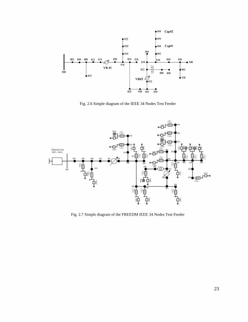
Fig. 2.6 Simple diagram of the IEEE 34 Nodes Test Feeder

Fig. 2.7 Simple diagram of the FREEDM IEEE 34 Nodes Test Feeder

23

2.2.2 Component Models

1. Feeder line

Each line section is represented by a 3 3× impedance matrix, in which the non-zero off-

diagonal elements indicate that the coupling effect between phases is taken into

consideration.

For the FREEDM Notional feeder, since the original data of the line sections are all sequence

based value as shown in the table before, all lines are using the sequence model [13].

For the FREEDM IEEE 34 feeder, since the original data of the line sections are complete

model based, to guarantee the accuracy of the simulation complete models are used.

2. Load Tap Changer (LTC)

Fig. 2.8 Simple diagram of the simplified Notional Feeder

24

Since we assume the LTC at substation can successfully regulate the substation voltage to an

ideal value, the impedance of the substation transformer is not considered in the simulation.

Instead, we treat the node downstream next to substation as a slack bus with a constant

voltage to model the regulation effect of LTC at the substation. For FREEDM Notional

feeder system, as indicated in the Fig 1.13, there are two main feeders connected to the

substation. Since the substation node is assumed to be a slack bus, the power flow calculation

results of these two feeders are independent. Therefore, we can perform simulation on these

two feeders separately, i.e. we can treat them as two independent systems. Here, only

simulation of feeder 1 is done. A brief diagram of feeder 1 is shown in Fig. 2.8. For

FREEDM IEEE 34 nodes system, since there is only one main feeder, all nodes are kept.

3. Voltage Regulator

The voltage regulator is modeled as a tap-changing transformer with line-drop compensator

(LDC) integrated. The LDC is illustrated in Fig. 1.4.

The voltage parameters are set according to the original documents, seen in Tab. 2.2.

Tab. 2.2 VRs setting in FREEDM 34 Nodes system

Location PT Ratio CT Ratio Bandwidth Voltage Level R-setting X-setting VR1 814-850 120 100 2 122 2.7 1.6 VR2 852-832 120 100 2 124 2.5 1.5

A DPF program with VR controller logic can be seen in Fig. 2.9 (a). The detailed input and

output of DPF and VR controller can be seen in Fig. 2.9 (b).

25

Start

Run DPF Program

t = t + Δt

VR controller

Tap change completed?

Yes

EndNo

New tap position from VR controller?

No

Yes

Fig. 2.9 (a) A DPF program with VR controller logic

26

DPF Parameters of line, transformers,etc

Load condition Tap positions of VRs

Vmes

VR controllerVmes from DPF

System global time tVR time-delay settings

Tap positionStatus of tap change

completeness

Fig. 2.9 (b) Input and output of DPF and VR controller

4. Loads

All the loads are modeled as constant PQ nodes, without considering the distribution

transformers. Therefore all the voltage profiles are primary voltages.

In the 24-hour simulation of FREEDM Notional Feeder, the load at each node is a

conforming load, i.e. load at each node is a fixed percentage of the total system load. The

total load characteristics is seen as follows. The system load variation during a day is shown

in Fig. 2.10. However, the load profile of the FREEDM IEEE 34 nodes system is non-

conforming.

27

Fig. 2.10 Load Variation of the FREEDM Notional Feeder

5. PV

For PVs, only the real and reactive power output is considered, so PVs are also modeled as

constant PQ nodes without considering the inverters, etc. Thus, the effect of PV can by

modeled by subtracting PV output from the load.

On the FREEDM notional feeder, each residential customer has a rooftop PV system

installed, and each PV system can generate up to a maximum load of the residential unit.

Therefore, the total PV output at each node has a maximum generation which is the same as

its peak load value. In the 24-hour simulation, all PVs in this thesis are all modeled as

constant PQ nodes with a conforming character consistent with solar irradiation during a day.

The PV and load profile during a day is shown in Fig. 2.11.

On the FREEDM IEEE 34 nodes feeder, there are five PV systems connected, the daily

profile of PVs are generated in the same way.

28

Fig. 2.11 PV and load variation of the FREEDM Notional Feeder

6. SST

Different from a conventional distribution transformer, a solid state transformer (SST) is a

converter based transformer, which has the features of load voltage regulation, voltage sag

compensation, fault isolation, harmonic isolation and DC output, etc [8]. Besides these,

another main feature of the SST is that it can automatically work under unity power factor

without receiving any control commands. In the FREEDM notional feeder all distribution

transformers are SSTs. Since all the reactive load required on the secondary side will be

provided by its corresponding SST, the equivalent reactive load at each node is zero, ie

0injQ = . Thus, with the change of load and PV output condition, the reactive power

generated by SSTs can always guarantee a unity power factor at each node. This is the

FREEDM default Volt/Var control scheme. In this thesis, the SST model is simplified as an

29

ideal transformer with adjustable reactive power source. Therefore, the load, PV and SST at

one node can be lumped together as a PQ node with zero reactive power.

7. Shunt Capacitor

All shunt capacitors are fixed capacitors with a constant reactance based on the rating.

30

2.3 Assessment of Volt/Var Control on FREEDM Notional Feeder

The simulation platform and two test cases have been used to demonstrate the assessment

process. Also, a base case in which conventional VVC scheme is used to compare with

FREEDM Notional Feeder. The challenge in the assessment is covering all the possible

operating conditions. In this study a set of cases have been identified to address this

challenge and facilitate the calculation of performance metrics.

2.3.1 Case Studies

No PV penetration

Case 1:

In this case, the conventional control scheme is adopted. There are two shunt capacitors in

the system with details shown as in Tab. 2.3, also a LTC at substation to keep voltage at

Node #0 at 1.025 p.u. when the total load exceeds 5MW, otherwise at 1.0 p.u.. No feeder

voltage regulator or SST is applied in this conventional scheme. Only peak load condition

with no PV penetration is simulated in this case. Detailed peak load data can be seen in the

appendices.

Tab. 2.3 Capacitor Ratings in IEEE 34 Nodes system

Location Capacity per phase (kVar) Node #5 400 Node #8 200

31

Case 2:

In this case, the FREEDM default control scheme is adopted. The reactive power injection at

each SST, injQ , is set as zero. Both capacitors are removed from the system. Voltage at the

substation is regulated at 1.0 p.u.. The load and PV condition is the same as in Case 1.

Simulation results and comparison between Case 1 and Case 2.

1. Voltage Profile

For the conventional control case the maximum voltage magnitude is 1.03 p.u. and the

minimum is 0.96p.u.. Therefore, the conventional VVC scheme is able to obtain the primary

goal of keeping voltages within the range of 0.95-1.05 p.u.. The total power loss of the

system is less than 2%, which is not a high value. In the default control case, the maximum

voltage is 1.01 p.u. and the minimum voltage is 0.96 p.u., which indicates that the FREEDM

Notional Feeder successfully solves the issue of voltage violation as well. Fig. 2.12 shows

the three-phase voltages along the feeders under the peak load condition.

32

Fig. 2.12 (a)

Fig. 2.12 (b)

33

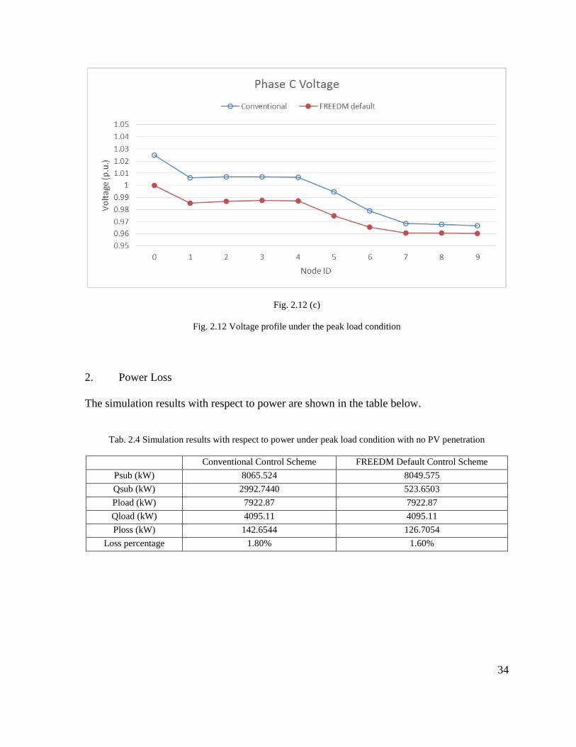
Fig. 2.12 (c)

Fig. 2.12 Voltage profile under the peak load condition

2. Power Loss

The simulation results with respect to power are shown in the table below.

Tab. 2.4 Simulation results with respect to power under peak load condition with no PV penetration

Conventional Control Scheme FREEDM Default Control Scheme Psub (kW) 8065.524 8049.575 Qsub (kW) 2992.7440 523.6503 Pload (kW) 7922.87 7922.87 Qload (kW) 4095.11 4095.11 Ploss (kW) 142.6544 126.7054

Loss percentage 1.80% 1.60%

34

From the simulation results above, the power loss percentage in FREEDM default control

(the proportion of power loss in total load) is 1.5992%, less than 1.8005% in conventional

case. The FREEDM VVC on Notional Feeder can reduce more power loss.


The FREEDM Notional feeder has two feeder ends, Node 4 and Node 9. The voltage

regulation at these two ends are shown in the figures below. The voltage regulation of the

system is the maximum value of the % regulation at all feeder ends. The three phase system

voltage regulation is seen in Fig. 2.13. These figures indicate that the FREEDM default

control scheme has less %Regulation than the conventional control scheme. The VRI under

FREEDM control is 4.14% in Phase C, while under conventional control the value is 7.29%

in Phase A. The FREEDM default control scheme reduce VRI by 43.27%.

Fig 2.13 (a)

35

Fig. 2.13 (b)

Fig. 2.13 (c)

Fig. 2.13 Voltage regulation under peak load condition

4. Voltage Unbalance

Since the load on the Notional Feeder is highly unbalanced, we need to investigate how the

FREEDM VVC influences the voltage unbalance at each node.

36

From the simulation result shown in Fig 2.14, we can see that for each node VU in the

system using the FREEDM default VVC is always less than that using conventional VVC.

The VUI under conventional control is 0.065, while under FREEDM default control is 0.042.

The FREEDM default control reduces the system voltage unbalance by 36.19%. Therefore,

FREEDM VVC mitigates the issue of voltage unbalance.

Fig. 2.14 Voltage Unbalance under peak load condition with no PV penetration

Case 3：

In this case, a 24-hour simulation is conducted to explore if the FREEDM VVC is still

effective when load varies during a day. Both the FREEDM VVC and the conventional VVC

are simulated to compare the effectiveness of the two control schemes.

The 24-hour simulation results are as follows:

37

1. Voltage Profile

Under FREEDM default control, the minimum voltage is 0.9602 pu at Node 9 in phase C at

18:30. The maximum voltage is 1.0053 p.u. at Node 5 in phase B at 18:30 as well. The

FREEDM VVC scheme successfully keep the voltages within the range 0.95-1.05 p.u. in

spite of the load variation during a day. 24-hour voltage profiles at Node 9 and 5 are shown

in Fig. 2.15.

Fig. 2.15 (a)

38

Fig. 2.15 (b)

Fig. 2.15 24-hour voltage profile at Node 5 and Node 9


Under FREEDM default control, the 24-hour primary-side power loss ranges from 21.91kW

at 3:00 to 126.71kW at 18:30, with a loss percentage range of 0.66%-1.60% respectively.

Under FREEDM default control the line currents in each phase are lower than those in the

conventional case, thus less power loss. Under conventional control the primary-side power

loss is always higher during a day, which indicates the FREEDM VVC mitigates the issue of

power loss better. From Fig. 2.16, the power loss shows the same pattern as the load

condition of the system, which verify that as load goes up power loss increases.

39

Fig. 2.16 Power loss during a day without PV penetration

Power loss characteristics with respect to load condition with a range from 40% to 110% can

be seen in Fig. 2.17. We can find a positive correlation between relationship between load

condition and loss percentage and this relationship is almost linear.

40

Fig. 2.17 Power loss characteristic with respect to load condition

Under FREEDM default control, as shown in Tab. 2.5, the primary-side energy loss is

1612.869 kWh for a day, which is less than 1767.756 kWh under conventional control. Thus,

the FREEDM default control can reduce primary-side energy loss as well. Energy loss

percentage in the table is defined as the proportion of energy loss in total load consumption.

The sum of both primary-side and secondary-side energy loss is 3123.093 kWh under

conventional VVC, and 5678.881 kWh under FREEDM default control. Thus, the FREEDM

default control can reduce primary-side energy loss, but it increases the total loss on both

primary and secondary sides.

Tab. 2.5 Daily primary-side energy loss without PV penetration

Conventional FREEDM default Energy loss for one day (kWh) 1767.756

1612.869

Energy loss percentage (%) 1.304292 1.190013

41


During the 24 hours, the maximum voltage regulations in both conventional control and

FREEDM default control cases occur under peak load condition. Thus the reduction of VRI

during a day is the same with the VRI reduction in the peak load condition simulation. As

shown in Fig. 2.18, for most of the time during a day %Regulation of the feeder under

FREEDM control is less than that under conventional control. Even though, around 3:00 the

%Regulation under FREEDM control is higher than that under conventional control, the

difference is very small.

Fig. 2.18 (a)

42

Fig 2.18 (b)

Fig. 2.18 (c)

Fig. 2.18 The system voltage regulation profile during a day without PV penetration

43

Fig. 2.19 System voltage regulation per phase during a day without PV penetration


From the 24-hour simulation results, for all the nodes, the voltage unbalance under FREEDM

default control is lower than the voltage unbalance under conventional control. And among

all the nodes, Node 9 always has the biggest voltage unbalance during 24 hours. From Fig.

2.20, we can find that at Node 9 voltage unbalance under FREEDM default control is always

lower than that under conventional control. Therefore, the FREEDM default control better

reduces the voltage unbalance of the system. The simulation results also shows that for each

node the maximum voltage unbalance occurs at peak load condition. In this 24-h simulation

the VUI is 0.0652 in conventional case and 0.0416 in FREEDN default control case. The

FREEDM default control reduce the VUI by 36.2%. Other voltage unbalance indices are also

calculated, as shown in Tab. 2.6.

44

Fig. 2.20 24-hour voltage unbalance at Node 9 without PV penetration

Tab. 2.6 Voltage Unbalance Index of Notional Feeder for zero PV case

VVC VUI (p.u.) %PVUR Index %VUF Index Zero PV Conventional 0.06520 4.04060 1.08194

FREEDM default 0.04160 2.29597 0.81636 5. Voltage Variation

Since for each node, we care about the voltage under different operating condition, the

Voltage Variation (VV) on primary side at all the nodes are calculated and shown in Fig.

2.21. Since in conventional control scheme, the LTC at substation regulates voltage at Node

0 at 1.0 and 1.025 p.u., for the nodes whose voltage does not depend much on load

conditions, the voltage variation is close to 0.025 shown as the figure for phase B. But under

FREEDM control the substation voltage is always 1.0 p.u., which makes the voltage

variation get rid of the tap changing effect of LTC at substation. Thus, for phase B the

45

FREEDM control reduces the voltage variation greatly. For each node, the VV’s under

FREEDM control is smaller than that under conventional control. The maximum VVI under

FREEDM control is 0.0236 p.u., under conventional control is 0.0313 p.u., shown as in Tab.

2.7. The FREEDM default control reduces the maximum VVI by 24.39%. As to the voltage

variations on the secondary-side, at each node with SST the VV is zero, since the SST can

regulate the secondary-side voltage constant [8]. In conventional distribution systems, in

which traditional distribution transformers are used, the voltage variations on the secondary-

side is the same as those on the primary-side. This is due to the assumption of an almost

constant voltage drop through the distributed transformer under different operation

conditions.

The histogram of primary-side voltages under conventional VVC are shown in Fig. 2.3. The

histogram of primary-side voltages under FREEDM default VVC are shown in Fig. 2.22.

Fig 2.21 (a)

46

Fig 2.21 (b)

Fig. 2.20 (c)

Fig. 2.21 Voltage Variation without PV penetration

47

Fig. 2.22 Histogram of voltages on the primary-side of the Notional feeder under FREEDM default VVC (zero

PV)

Tab. 2.7 VVI comparison with no PV penetration

Control VVI_a VVI_b VVI_c Max(VVI) Conventional 0.0151 0.0032 0.0236 0.0236

FREEDM default 0.0313 0.0250 0.0254 0.0313

High PV penetration

Since there is no PV output during the peak load time 18:30, all the simulations under the

peak load condition have the same results with Case 1 and Case 2. Therefore, with PV

penetration, the FREEDM VCC is still effective under peak load condition.

0.96 0.97 0.98 0.99 1 1.01 1.020

50

100

150

200

250

300

350

Voltage (p.u.)

Freq

uenc

y

Voltage Histogram

mean= 0.9908standard deviation=0.0102

48

Case 4:


effective when there is high PV penetration in the system.

1. Voltage Profile

Under FREEDM default control, the minimum voltage is 0.9602 p.u. at Node 9 in phase C at

18:30. The maximum voltage is 1.0084 p.u. at Node 9 in phase C at 12:00 when the PV

output exceeds the load which leads to a reverse power flow. Phase C voltage at Node 9 is

shown in Fig. 2.23.

Fig. 2.23 Phase C voltage at Node 9 during a day with high PV penetration

Both the maximum and minimum voltages during a day is within the required range,

indicating the FREEDM VVC successfully regulating the voltages if PVs are connected to

the system. The simulation results of voltage profiles under conventional control is also

49

within the required range. Phase C voltage at Node 9 under conventional control is included

in the figure below as well. The abnormal voltage change in the conventional control case

around 7:00 and 15:00 o’clock is due to the tap change of LTC at substation.

2. Power Loss and Energy loss

Under FREEDM default control, the 24-hour primary-side power loss ranges from 0.0877kW

at 9:30 to 126.71kW at 18:30. From Fig. 2.24, we can see that under conventional control the

primary-side power loss is always higher during a day, which indicates the FREEDM VVC

mitigates the issue of power loss better. Under FREEDM default control the line currents in

each phase are lower than that in the conventional case, thus less power loss. Although the

system load in both case are high during the daytime, PVs help to reduce the power loss.

Fig. 2.24 Power loss during a day with high PV penetration

50

As shown in Tab. 2.8, under FREEDM default control, the energy loss is 1043.161 kWh for a

day, which is less than 1183.144 kWh under conventional control. Thus, the FREEDM

default control can reduce energy loss if the system has PVs connected as well. Energy loss

percentage in the table is defined as the proportion of energy loss in total load consumption.

The sum of both primary-side and secondary-side energy loss is 4124.320 kWh under

conventional VVC, and 3680.209 kWh under FREEDM default control. Thus, the FREEDM

default control can reduce both primary-side and secondary-side energy loss.

Tab. 2.8 Daily energy loss with high PV penetration

Conventional FREEDM default Energy loss for one day (kWh) 1183.144

1043.161

Energy loss percentage (%) 0.872952

0.769669


In the results of 24-hour simulation, some of the % Regulations of the feeder are negative,

because voltage rises along the feeder. The voltage rise along the feeder can result from

either reverse power flow, or highly unbalance of the system or both. For Phase A and Phase

C, the maximum voltage regulations in both control cases occur under peak load condition, at

18:30. For Phase B the maximum absolute value of %Regulation under conventional control

is under peak PV output condition, at 12:00, while in FREEDM default control case the

maximum %Regulation still occurs at 18:30. For most of the time during a day the absolute

value of %Regulation of the feeder under FREEDM control is less than that under

conventional control.

51

A comparison of maximum absolute value %Regulation during 24 hours is shown in the Fig.

2.25. The VRI under conventional control is 7.29%, under FREEDM control is 4.14%. The

FREEDM reduce the VRI by 43.27%.

Fig. 2.25 (a)

Fig. 2.25 (b)

52

Fig. 2.25 (c)

Fig. 2.25 System voltage regulation per phase during a day with high PV penetration

Fig. 2.26 Maximum voltage regulation during a day with high PV penetration

53


As to voltage unbalance, the simulation results for system with PV shows that Node 9 always

has the biggest voltage unbalance during 24 hours. From the Fig. 2.27, we can find that at

Node 9, voltage unbalance under FREEDM default control is always lower than that under

conventional control. The maximum voltage unbalance during a day also occurs under peak

load condition, thus the reduction of VVI is also 36.2%. Therefore, the FREEDM default

control better reduces the voltage unbalance of the system. Other voltage unbalance indices

are also the same in zeros PV case, shown in Tab. 2.6

Fig. 2.27 Voltage unbalance at Node 9 during a day with high PV penetration

5. Voltage Variation

The voltage variation for each node and each phase is shown in Fig. 2.28. Since in

conventional control scheme, the LTC at substation regulates voltage at Node 0 at 1.0 and

54

1.025 p.u., the voltage variation at some nodes is much larger than 0.025 p.u.. That is because

at noon the PV output exceeds the system load, and the consequent reverse power flow

makes the maximum voltage larger than 1.025 p.u., even though the LTC at substation still

regulates voltage at Node 0 to 1.0 p.u.. At the same time the minimal voltage remains the

same as in zero-PV case. Thus, the variation is larger than that in zero-PV case. But in

FREEDM control case the maximal voltage due to the reverse power flow is close to 1.0 p.u.,

while the minimal voltage is close to that in conventional control case, thus the voltage

variation is lower.

The maximum VVI under FREEDM control is 2.36%, under conventional control is 3.13%.

The FREEDM control reduce the VVI by 24.39%. The results is the same as those in non-PV

cases, shown as in Tab. 2.9. As to the voltage variations on the secondary-side, at each node

with SST the VV is zero, since the SST can regulate the secondary-side voltage constant [8].

In conventional distribution systems, in which traditional distribution transformers are used,

the voltage variations on the secondary-side is the same as those on the primary-side.



55

Fig. 2.28 (a)

Fig. 2.28 (b)

56

Fig. 2.28 (c)

Fig. 2.28 Three-phase voltage variation during a day with high PV penetration

Tab. 2.9 VVI comparison with high PV penetration

Control VVI_a VVI_b VVI_c Max(VVI) FREEDM 0.0272 0.0064 0.0481 0.0481

Conventional 0.0743 0.0250 0.0634 0.0743

57

Fig. 2.29 Histogram of voltages on the primary-side of the Notional feeder under conventional VVC (high PV)

Fig. 2.30 Histogram of voltages on the primary-side of the Notional feeder under conventional VVC (high PV)

0.95 0.96 0.97 0.98 0.99 1 1.01 1.02 1.03 1.040

50

100

150

200

250

300

Voltage (p.u.)

Freq

uenc

y

Voltage Histogram


0.96 0.97 0.98 0.99 1 1.01 1.020

100

200

300

400

500

600

700

Voltage (p.u.)

Freq

uenc

y

Voltage Histogram


58

2.3.2 Summary

1. The primary-side voltages in the system can be regulated within the recommended

service voltage range of 0.95-1.05 p.u. (range A by ANSI C84.1) under both the conventional

and FREEDM default control schemes. Even when there is high PV penetration in the sytem,

the voltages are still within the required range under both Volt/Var control schemes.

2. Under peak load condition, the primary-side power loss under the conventional

control is 142.65kW; with the FREEDM default control the primary-side power loss is

126.71kW. A reduction of 11.17% is achieved. For a typical day, with minimum (zero) PV

output, the primary-side energy loss under conventional control is 1767.8kWh, under

FREEDM default control is 1612.9kWh. The FREEDM default control reduces primary-side

energy loss by 8.76%. With full PV penetration (peak PV generation at each node equals

peak load), the primary-side energy loss under the conventional control is 1183.1kWh, under

FREEDM default control is 1043.2kWh. A reduction of 11.83% is achieved. When

considering the secondary-side loss, the FREEDM VVC has more total energy loss than the

conventional control in a zero-PV day, but less total energy loss in a high-PV day.

3. The FREEDM default control greatly reduces the voltage regulation of the feeder.

The VRI under conventional control is 7.29%, under FREEDM control is 4.14%. A reduction

of 43.27% is achieved by the FREEDM default control scheme.

4. The FREEDM default control greatly reduces the voltage unbalance of the system.

The VUI is 0.0652 p.u. under the FREEDM default control, and 0.0416 p.u. under

conventional control. A reduction of 36.2% is achieved by the FREEDM default control

scheme.

59

5. The FREEDM default control also reduces the voltage variation on the primary-side

under different operating conditions during a day. In a zero-PV day, the maximum VVI

among three phases is 0.0236 p.u. under FREEDM default control, and 0.0313 p.u. under

conventional control. The FREEDM default control scheme achieves a voltage variation

reduction of 24.39%. In a high-PV day, the maximum VVI among three phases is 0.0481 p.u.

under FREEDM default control, and 0.0743 p.u. under conventional control. The FREEDM

default control scheme achieves a voltage variation reduction of 35.29%. Besides, the

FREEDM control guarantees a zero voltage variation on the secondary-side.

60

2.4 Assessment of Volt/Var Control on FREEDM IEEE 34 Nodes Feeder

Similar to the FREEDM Notional Feeder, the FREEDM IEEE 34 Nodes Feeder also use

SSTs to accommodate all loads and PVs. There are two VRs in the system, connected

between node 814 and 850, 852 and 832.

2.4.1 Case Studies

No PV penetration

Case 0:

In this case, no Volt/Var control scheme is applied. Both voltage regulators and capacitors

are removed from the conventional IEEE 34 Nodes feeder. This case is simulated to prove

the necessity to apply VVC on this feeder.

Since under peak load condition, the system will have the largest voltage drop and power

loss, to further investigate the effectiveness of FREEDM Volt/Var control scheme under the

worst case, Case 1 and Case 2 are developed.

Case 1:

In this case, the conventional control scheme is applied. Besides the two voltage regulators as

mentioned before, there are two fixed capacitor banks in IEEE 34 system, with the detailed

data shown in Tab. 2.10.

61

Tab. 2.10 Capacitor data for IEEE 34 System

Cap # Connected to IQL A(kVAR) IQL B (kVAR) IQL C (kVAR) 1 844 100 100 100 2 848 150 150 150

Case 2:

In this case, the FREEDM default control scheme is applied. The reactive power injection at

each SSTs, injQ is set as zero. Capacitors are removed, but VRs are kept.

The simulation results of these three cases under peak load condition are seen as follows.

1. Voltage Profile

Since ANSI C 84.1 range A voltage is limited to service voltage, only voltages on primary

side are compared with range A, 0.95-1.05 p.u.. In FREEDM IEEE 34 nodes system, Node

888 and 890 are on the secondary side of the distribution transformer located between Node

832 and 888, thus their voltage profiles are not considered.

As illustrated in Fig. 2.31, in Case 0, voltages at many nodes are lower than 0.95, thus it is

necessary to apply Volt/Var Control scheme to regulate the voltages in the system. In case 1,

under conventional control scheme, the maximum voltage is 1.05 p.u. and the minimum is

0.961p.u.. The conventional VVC scheme is able to obtain the primary goal of keeping

voltages within the range of 0.95-1.05 p.u.. In case 2, under FREEDM default VVC, the

maximum voltage is 1.05 p.u. and the minimum is 0.971 p.u.. which indicates that the

FREEDM VVC successfully solves the issue of voltage violation as well.

62

Fig 2.31 (a)

Fig. 2.31 (b)

63

Fig. 2.31 (c)

Fig. 2.31 Feeder Voltage profile under peak load condition

2. Power Loss

The simulation results with respect to power are shown in Tab. 2.11.

Tab. 2.11 Simulation results with respect to power under peak load condition

No VVC Conventional Control

FREEDM Default

Psub 1800.731 1701.581 1680.42 Qsub 1077.209 326.575 141.6328 Pload 1496.651 1496.651 1496.651 Qload 857.7689 857.769 857.769 Ploss 304.0802 204.9306 183.769

Loss percentage 20.32% 13.69% 12.28%

Both Conventional and FREEDM VVC can reduce the power loss, and the power loss

percentage under FREEDM VVC is 12.28%, which is smaller than that in case 1, under

conventional VVC. Thus, under peak load condition, the FREEDM VVC can reduce more

power loss than conventional VVC in IEEE 34 nodes systems.

64


The IEEE 34 nodes feeder has eight feeder ends, Node 838, 810, 822, 826, 856, 864, 848 and

840. The voltage regulation at these eight ends are shown in Tab. 2.12 below. The voltage

regulation of the system is the maximum value of the % regulation at all feeder ends. As

shown in Fig. 2.32, the VRI under FREEDM control is 7.04%, which is less than 5.91%

under conventional control. The FREEDM VVC reduce the voltage regulation by 15.97%,

compared to the conventional VVC.

Tab. 2.12 Voltage regulation under peak load condition

%Regulation Conventional VVC FREEDM default VVC Phase A Phase B Phase C Phase A Phase B Phase C

838 4.023293 3.86973 810 1.741885 1.644932 822 7.037624 5.913467 826 3.180478 3.558937 856 4.725862 5.123481 864 3.643014 3.618383 848 3.715755 3.929307 4.593714 3.81824 3.849974 4.189102 840 3.81358 3.993094 4.719465 3.834366 3.847718 4.228905

65

Fig. 2.32 Feeder voltage regulation under peak load condition


Since the IEEE 34 nodes system is also a highly unbalanced system, we need to investigate

how the FREEDM VVC influences the voltage unbalance at each node.

From the simulation result shown in Fig. 2.33, we can see that both the conventional VVC

and the FREEDM VVC can reduce the VU at each node. The VUI under conventional

control is 0.0264 p.u., under FREEDM default control is 0.0222 p.u.. The FREEDM VVC

reduces VUI by 15.87 % compared with the conventional control.

66

Fig. 2.33 Voltage unbalance under peak load condition

Case 3:


effective when load varies during a day and there is no PV penetration.

The 24-hour simulation results are as follows:

1. Voltage Profile

From the simulation results, both control schemes successfully keep the voltages within the

range 0.95-1.05 p.u. in spite of the load variation during a day. Under FREEDM default

control, the minimum voltage is 0.9676 pu at Node 852 in phase C at 18:00. Under

conventional control, the minimum voltage is 0.9614 p.u. at Node 852 in phase C at 18:30.

67

The maximum voltage is 1.05 p.u at the substation in both cases. The 24-hour voltage profile

at Node 852 is shown in Fig 2.34.

Fig. 2.34 Voltage at Node 852 during a day without PV penetration


As shown in Fig. 2.35, under FREEDM default control, the 24-hour power loss ranges from

28.92kW at 3:00 to 183.769kW at 18:30, with a loss percentage range of 4.52%-12.28%

respectively. Under conventional control the power loss is always higher during a day, which

indicates that the FREEDM VVC mitigates the issue of power loss better. In Fig. 2.35, the

power loss shows the same pattern as the load condition of the system, which verifies that as

the load goes up the power loss increases. From, Tab. 2.13, under FREEDM default control,

the energy loss is 2263.181kWh for a day, which is less than 2505.465kWh under

conventional control. The sum of both primary-side and secondary-side energy loss is

68

2761.690 kWh under conventional VVC, and 3033.079 kWh under FREEDM default

control. Thus, the FREEDM default control can reduce primary-side energy loss, but it

increases the total loss on both primary and secondary sides.

Fig. 2.35 Power loss during a day without PV penetration

Tab. 2.13 Daily energy loss without PV penetration

Conventional FREEDM default Energy loss for one day (kWh) 2505.465 2263.181



In the results of 24-hour simulation, for Phase A, the maximum voltage regulations in both

control cases occur are under peak load condition, at 18:30, 7.03% under conventional VVC,

5.91% under FREEDM default VVC. For Phase B the maximum %Regulation under

69

conventional control is 5.09% at 9:30 AM, while in FREEDM default control case the

maximum %Regulation is 5.12% at 18:30, slightly more than the value under conventional

control. For Phase C, the maximum %Regulation under conventional control is 4.72% at

18:30, while in FREEDM default control case the maximum %Regulation in the same phase

occurs at 18:00 with a value of 4.58%. A comparison of maximum %Regulation at each

phase during 24 hours is shown in Fig. 2.36. The VRI under conventional control is 7.03%,

under FREEDM control is 5.91%. The FREEDM VVC reduce the VRI by 15.97%.

Fig. 2.36 (a)

70

Fig. 2.36 (b)

Fig. 2.36 (c)

Fig. 2.36 The system voltage regulation profile during a day without PV penetration

71

Fig. 2.37 System voltage regulation per phase during a day without PV penetration


From the 24-hour simulation results, for some nodes the voltage unbalance under the

FREEDM default control is always less than that under the conventional control. Such

phenomenon at Node 814 is shown in Fig. 2.38. However, for other nodes the voltage

unbalance under the FREEDM default control is not always less than that under the

conventional control, as illustrated in Fig.2.39. The VUI is 0.0284 p.u. in conventional

control case and 0.0222 p.u. in FREEDN default control case. The FREEDM default control

reduce the VUI by 21.8%. Other voltage unbalance indices are shown in Tab. 2.14

72

Fig. 2.38 Voltage unbalance at Node 814 during a day without PV penetration

Fig. 2.39 Voltage unbalance at Node 852 during a day without PV penetration

73

Tab. 2.14 Voltage Unbalance Index of Notional Feeder for zero PV case

VVC VUI %PVUR Index %VUF Index Zero PV Conventional 0.02842 1.45710 0.77464

FREEDM default 0.02224 1.17134 0.67934


The voltage Variations (VVs) at each node, under different VVC are shown in Fig. 2.40.

Under the FREEDM default VVC, the VVs at each node during a day is always less than

those under the conventional VVC. The maximum VVI under FREEDM control is 0.0420

p.u., under conventional control is 0.0573 p.u., shown as in the table below. The FREEDM

default control reduces the maximum VVI by 26.70%. As to the voltage variations on the

secondary-side, at each node with SST the VV is zero, since the SST can regulate the

secondary-side voltage constant [8]. In conventional distribution systems, in which

traditional distribution transformers are used, the voltage variations on the secondary-side is

the same as those on the primary-side.



Tab. 2.15 VVI comparison with no PV penetration


FREEDM default 0.0420 0.0361 0.0405 0.0420

74

Fig. 2.40 (a)

Fig. 2.40 (b)

75

Fig. 2.40 (c)

Fig. 2.40 Voltage Variation without PV penetration

Fig. 2.41 Histogram of voltages on the primary-side of the IEEE 34 feeder under conventional VVC (zero PV)

0.96 0.98 1 1.02 1.04 1.06 1.080

200

400

600

800

1000

1200

1400

Voltage (p.u.)

Freq

uenc

y

Voltage Histogram


76

Fig. 2.42 Histogram of voltages on the primary-side of the IEEE 34 feeder under FREEDM default VVC (zero

PV)

6. Voltage Regulator Tap Change

Voltage regulators change tap positions corresponding to the load variations during a day,

Fig. 2.43 shows the tap positons of the two voltage regulators under both control scheme

during a day. The Voltage Regulator Tap Change of the two voltage regulators are shown in

Tab.2.12. For either voltage regulator, the tap position changes under FREEDM control is

always less or equal to those under the conventional default control. The VRTCI of those two

voltage regulators has the same trend, as shown in Tab.2.17.

The number of operations of the two VRs are shown in Tab. 2.17.

0.96 0.98 1 1.02 1.04 1.06 1.080

200

400

600

800

1000

1200

1400

Voltage (p.u.)

Freq

uenc

y

Voltage Histogram


77

Fig. 2.43 (a) VR1

Fig. 2.43 (b)VR2

Fig. 2.43 Phase A tap positions of the two VRs during a day without PV penetration

78

Tab. 2.16 Tap change of the VRs during a day without PV penetration

VRTC VVC Phase A Phase B Phase C VRTCI VR1 Conventional 7 5 6 7

FREEDM default 5 3 5 5 VR2 Conventional 5 4 6 6

FREEDM default 5 4 4 5

Tab. 2.17 Number of operations of the VRs during a day without PV penetration

#Operations VVC Phase A Phase B Phase C #Op Index VR1 Conventional 16 13 14 16



High PV Penetration

Since there is no PV output during the peak load time, 18:30, and the tap positions of the two

voltage regulators remain the same as those in Case 3. Therefore, all simulations under the

peak load condition have the same results with Case 3. For the system with PV connected,

the FREEDM VCC is still effective under peak load condition.

Case 4:


effective when there is high PV penetration in the system.

The corresponding simulation results are as follows.

79

1. Voltage Profile

Under the conventional control, primary-side voltages ranges from 0.9614p.u. to 1.0628p.u..

The maximum voltage occurs at Node 814 in Phase C at noon. Under the FREEDM default

control, primary-side voltages ranges from 0.9676p.u. to 1.0604p.u.. The maximum voltage

occurs at Node 814 in Phase C at noon as well. In both cases, the system suffers voltage

violations. The regulating points of the two voltage regulators are both downstream of the

voltage regulators. However, Node 814 is located upstream of the voltage regulators, and

Node 800 is regulated at 1.05 p.u. by the LTC at substation. At noon the PV generation

exceeds the load, resulting in reverse power flow. When power goes from Node 814 to Node

800, the voltage at Node 814 will be higher than the voltage at Node 800, thus violating the

upper voltage limit. The 24-hour Phase C voltage profile at Node 814 is shown in Fig. 2.44.

Fig. 2.44 Phase C voltage profile at Node 814 with high PV penetration

80


As shown in Fig. 2.45, under FREEDM default control, the 24-hour power loss ranges from

3.82kW at 13:30 to 204.12kW at 18:30, with a loss percentage range of 0.37%-12.28%

respectively. Under conventional control the power loss is always higher during a day, which

indicates the FREEDM VVC mitigates the issue of power loss better. Under FREEDM

default control, the primary-side energy loss is 1500.725kWh for a day, which is less than

1726.457kWh under conventional control. The sum of both primary-side and secondary-side

energy loss is 1913.175 kWh under conventional VVC, and 2061.774 kWh under FREEDM

default control. Thus, the FREEDM default control can reduce primary-side energy loss, but

it increases the total loss on both primary and secondary sides.

Fig. 2.45 Power loss during a day with high PV penetration

81

Tab. 2.18 Daily energy loss with high PV penetration

Conventional FREEDM default Energy loss for one day (kWh) 1726.457131 1500.724528



In the results of 24-hour simulation, for Phase A, the maximum voltage regulations in both

control cases occur under peak load condition, at 18:30, 7.03% under conventional VVC,

5.91% under FREEDM default VVC. For Phase B the maximum %Regulation under

conventional control is 4.91% at 17:30, while in FREEDM default control case the maximum

%Regulation is 5.12% at 18:30. For Phase C, the maximum %Regulation under conventional

control is 4.72% at 18:30, while in FREEDM default control case the maximum %Regulation

in the same phase occurs at 18:00 with a value of 4.58%. A comparison of maximum

%Regulation at each phases during 24 hours is shown in Fig. 2.46. The VRI has the same

results as the system with zero PV penetration. The FREEDM VVC still reduces the VRI by

15.97% if the PV penetration is high.

82

Fig. 2.46 (a)

Fig. 2.46 (b)

83

Fig. 2.46 (c)

Fig. 2.46 The system voltage regulation profile during a day with high PV penetration

Fig. 2.47 System voltage regulation per phase during a day with high PV penetration

0

1

2

3

4

5

6

7

8

Phase A Phase B Phase C

% R

egul

atio

n

System Voltage Regulation

Conventional FREEDM default

84


From the 24-hour simulation results, for all the nodes, the voltage unbalance under the

FREEDM default control is not always less than that under the conventional control. Such

phenomenon at Node 814 and Node 852 is shown in Fig. 2.48. However, VUIs are the same

as the results of zero-PV penetration case. The VUI is 0.0284 p.u. in conventional control

case and 0.0222 p.u. in FREEDM default control case. The FREEDM default control reduces

the VUI by 21.8%. Other voltage unbalance indices are shown in Tab. 2.19

Fig. 2.48 (a) Voltage unbalance at Node 814 during a day with high PV penetration

85

Fig. 2.48 (b) Voltage unbalance at Node 814 during a day with high PV penetration

Tab. 2.19 Voltage Unbalance Index of Notional Feeder for high PV case

VVC VUI %PVUR Index %VUF Index High PV

Conventional 0.02842 1.45710 0.77464 FREEDM default 0.02224 1.27064 0.72597


The voltage Variations (VVs) at each node, under different VVC are shown in Fig. 2.49.

Different from the results of case3 (the zero-PV penetration case), under the FREEDM

default VVC, the VVs at some nodes during a day are always less than those under the

conventional VVC. But for other nodes, such as Node 852, under the FREEDM default

VVC, the VVs in certain phase are higher than that under the conventional VVC. However,

the maximum VVI under FREEDM control is 0.0812 p.u., while under conventional control

86

is 0.08423 p.u., shown as in Tab. 2.20. The FREEDM default control still reduces the

maximum VVI, but with a smaller reduction of 3.56%.

As to the voltage variations on the secondary-side, at each node with SST the VV is zero,

since the SST can regulate the secondary-side voltage constant [8]. In conventional

distribution systems, in which traditional distribution transformers are used, the voltage

variations on the secondary-side are the same as those on the primary-side.

The histogram of primary-side voltages under conventional VVC is shown in Fig. 2.50. The

histogram of primary-side voltages under FREEDM default VVC is shown in Fig. 2.51.

Fig. 2.49 (a)

87

Fig. 2.49 (b)

Fig. 2.49 (c)

Fig. 2.49 Voltage Variation with high PV penetration

88

Tab. 2.20 VVI comparison with high PV penetration


FREEDM default 0.0702 0.0543 0.0812 0.0812

Fig. 2.50 Histogram of voltages on the primary-side of the IEEE 34 feeder under conventional VVC (high PV)

0.96 0.98 1 1.02 1.04 1.06 1.08 1.10

200

400

600

800

1000

1200

1400

1600

Voltage (p.u.)

Freq

uenc

y

Voltage Histogram


89

Fig. 2.51 Histogram of voltages on the primary-side of the IEEE 34 feeder under FREEDM default VVC (high

PV)

6. Voltage Regulator Tap Change

Fig 2.52 shows the tap positons of the two voltage regulators under both control schemes,

during a day. The Voltage Regulator Tap Change of the two voltage regulators are shown in

Tab.2.21. For either voltage regulator, under FREEDM control the tap position changes are

always less than those under the conventional default control. The VRTCIs of those two

voltage regulators have the same trend, as shown in Tab.2.21. From this point, the FREEDM

default VVC can still reduce the device cost when there is high PV penetration in the system.

The number of operations of the two VRs are shown in Tab. 2.22.

0.96 0.98 1 1.02 1.04 1.06 1.08 1.10

200

400

600

800

1000

1200

Voltage (p.u.)

Freq

uenc

y

Voltage Histogram


90

Fig. 2.52 (a)

Fig. 2.52 (b)

Fig. 2.52 Phase A tap positions of the two VRs during a day with high PV penetration

91

Tab. 2.21 Tap change of the VRs during a high-PV day

VRTC VVC Phase A Phase B Phase C VRTCI VR1 Conventional 10 6 9 10



Tab. 2.22 Number of operations of the VRs during a high-PV day

#Operations VVC Phase A Phase B Phase C #Op Index VR1 Conventional 22 15 18 22



2.4.2 Summary

1. The primary-side voltages in the system can be regulated within the recommended

service voltage range of 0.95-1.05 p.u. (range A by ANSI C84.1) under both the conventional

and FREEDM default control schemes. But when there is high PV penetration in the system,

the voltages violates the upper limit under both Volt/Var control schemes.

2. Under peak load condition, the primary-side power loss under the conventional

control is 204.93kW; with the FREEDM default control the power loss is 183.77kW. A

reduction of 10.33% is achieved. In a zero-PV day, the primary-side energy loss under

conventional control is 2505.5kWh, under FREEDM default control is 2263.2kWh. The

FREEDM default control reduces the primary-side energy loss by 9.67%. In a high-PV day,

the primary-side energy loss under the conventional control is 1726.5kWh, under FREEDM

default control is 1500.7kWh. A reduction of 13.07% is achieved. When considering the

92

secondary-side loss, the FREEDM VVC has more total energy loss than the conventional

control.

3. The FREEDM default control can reduce the voltage regulation of the feeder. The

VRI under conventional control is 7.03%, under FREEDM control is 5.91%. A reduction of

15.97% is achieved by the FREEDM default control scheme.

4. The FREEDM default control greatly reduces the voltage unbalance of the system.

The VUI is 0.0652 p.u. under the FREEDM default control, and 0.0416 p.u. under

conventional control. A reduction of 36.2% is achieved by the FREEDM default control

scheme.

5. The FREEDM default control also reduces the voltage variation on the primary-side

under different operating conditions during a day. In a zero-PV day, the maximum VVI

among three phases is 0.0573 p.u. under FREEDM default control, and 0.0420 p.u. under

conventional control. The FREEDM default control scheme achieves a voltage variation

reduction of 26.70%. In a high-PV day, the maximum VVI among three phases is 0.0842 p.u.

under FREEDM default control, and 0.0812 p.u. under conventional control. The FREEDM

default control scheme achieves a voltage variation reduction of 3.56%. Besides, the

FREEDM control guarantees a zero voltage variation on the secondary-side.

6. The FREEDM default control always has less VRTC for each phase than those under

conventional control, thus less control cost for the voltage regulators.

93

Chapter 3 Alternative Volt/Var Control Schemes for FREEDM

Systems

The objectives of Volt/Var control includes maintaining the voltages within acceptable

limits, reducing power and energy loss, and reducing voltage unbalance and variation. The

most common methods of Volt/Var Control are direct voltage regulation and Var

compensation. The load tap changer (LTC) and voltage regulator (VR) are such devices that

can regulate voltage directly like a transformer. Also for Var compensation, SSTs can be

used to provide reactive power support in FREEDM Systems. Thus alternative VVC schemes

can be designed for the FREEDM systems by utilizing these two methods.

The following subsections illustrate the adoption of these two methods for a given system.

3.1 Option I: Var Compensation for Volt/Var Control on FREEDM systems

This option uses only the Var compensation provide by SSTs on a FREEDM system. As

illustrated in previous chapter, SSTs operating at unity power factor alone provide a good

voltage profile for feeders with moderate voltage drop. In such cases, SSTs can provide extra

voltage boost when needed, and that may be enough to keep the voltages within limits.

Under FREEDM default control, the control variable injQ , also the reactive power injected at

each node is zero. With the increasing reactive power provided by SST the effectiveness of

Volt/Var control can be improved. This can be justified by the following two simulations.

94

Case 1: Var Compensation on the FREEDM Notional Feeder

In this case, the injQ from SSTs on the FREEDM Notional Feeder is changed from 0 to -50

kVar under peak load condition. The LTC at substation still regulate the voltage at Node 0 at

1.0 p.u..

Tab. 3.1-3.3 show the simulation results under peak load condition. These results show that

as injQ increases, the voltages at the nodes is boosted along the feeder, as expected, shown in

Fig. 3.1. Fig. 3.2 shows the %Regulation of Node 9.

Tab. 3.1 Simulation results for Case 1.1

Case 1.1: = 5injQ kVar− Node ID Va Vb Vc

0 1 1 1 1 0.983509 1.002017 0.986139 2 0.980886 1.000762 0.987764 3 0.980823 1.000158 0.98823 4 0.981063 1.00003 0.988075 5 0.97905 1.006035 0.975749 6 0.977962 1.00619 0.966693 7 0.977934 1.003381 0.962034 8 0.977873 1.003205 0.961746 9 0.977535 1.002981 0.961463 Total

Psub (kW) 3140.88 2427.136 2481.347 8049.363 Qsub (kVar) 240.3677 62.38758 89.98993 392.7453 Pload (kW) 3083.85 2433.54 2405.48 7922.87 Ploss (kW) 57.02978 -6.40408 75.86709 126.4928

Loss percentage 1.5966%

95



0 1 1 1 1 0.984916 1.003813 0.988118 2 0.982381 1.002821 0.990049 3 0.982319 1.002376 0.990718 4 0.982607 1.002296 0.99061 5 0.981029 1.008386 0.978318 6 0.980464 1.009058 0.96981 7 0.980804 1.006623 0.965534 8 0.980763 1.006467 0.965266 9 0.980461 1.006278 0.965019 Total

Psub (kW) 3143.315 2426.456 2479.281 8049.052 Qsub (kVar) 119.0954 -70.2148 -47.481 1.399573 Pload (kW) 3083.85 2433.54 2405.48 7922.87 Ploss (kW) 59.46505 -7.08432 73.80138 126.1821


Fig. 3.1 Phase C voltage at Node 9

96



0 1 1 1 1 0.987713 1.007378 0.992037 2 0.985354 1.006908 0.994579 3 0.985293 1.006778 0.995648 4 0.985678 1.006795 0.995637 5 0.984961 1.013049 0.983408 6 0.985432 1.014747 0.975979 7 0.986503 1.013053 0.972461 8 0.986502 1.012938 0.972235 9 0.986272 1.012819 0.972059 Total

Psub 3148.511 2425.781 2475.584 8049.876 Qsub -121.804 -333.396 -320.042 -775.242 Pload 3083.85 2433.54 2405.48 7922.87 loss 64.66075 -7.75911 70.10388 127.0055


97

Fig. 3.2 Phase A %Regulation at Node 9 during a day without PV penetration

As to power loss, the loss percentage goes down from 1.597% to 1.593% as injQ goes from -

5kVar to -20kVar. But it then increases to 1.603% as injQ goes to -50kVar. The absolute

value of power loss also decreases first then increases as SSTs provide more reactive power.

Simulations for injQ ranges from 0 to -50kVar, with a gap of 5kVar are all conducted. The

respective results are seen in Fig. 3.3. From the graph, we can find some optimal value of

injQ to achieve a minimal power loss.

98

Fig. 3.3 Power loss characteristic with respect to injQ

In case 1, for the FREEDM notional feeder, we found that Node 9 always has the most

Voltage Unbalance and Voltage Variation. Although we change injQ from 0 to -40kVar, there

is little change of voltage unbalance and variation as shown in Fig. 3.4 and Fig. 3.5. It seems

that we can design an alternative VVC scheme by just increase the reactive power injected by

SST in order to reduce power loss further.

99

Fig. 3.4 Voltage unbalance at Node 9 for different injQ

Fig. 3.5 Voltage variation at Node 9 for different injQ

100

Case 2: Var Compensation on the FRREDM IEEE 34 Nodes Feeder

In this case, the injQ on the FREEDM IEEE 34 Nodes Feeder is changed from 0 to -20 kVar

under peak load condition. The LTC at substation still regulate the voltage at Node 800 at

1.05 p.u.. And the tap position of the two VRs are kept as in Case 2 of the FREEDM IEEE 34

Nodes Feeder.

Case 2.1: In this case, = 5injQ kVar− under peak load condition.




As in previous case, increasing the injQ boosts the voltages on the feeder. Fig.3.6 shows the

phase C voltage profiles at Node 852 with increasing injQ . In case 2.1, 2.2 and 2.3, all

voltages are within the range 0.95 p.u.-1.05 p.u. In case 2.4, voltage at Node 832, Phase B

exceeds 1.05 p.u., indicating that over Var injection by SSTs would result in voltage

violation. . Among all feeder ends, Node 822 always has the maximum %Regulation as the

change of injQ . %Regulation at Node 822 decreases as SSTs inject more reactive power, as

illustrated in Fig. 3.7. Unlike the Notional Feeder, on which injQ has little influence on the

voltage, in the IEEE 34 Nodes system injQ have certain effect on the voltage profile. Hence,

we can design an alternative VVC scheme for the FREEDM IEEE 34 Nodes Feeder by

increasing injQ .

101

As to power loss, the loss percentage goes down from 12.279% to 12.123% as injQ goes from

0kVar to -5kVar. But it then increases to 13.570% as injQ goes to -20kVar. This

characteristic is shown in Fig. 3.8. The absolute value of power loss also decreases first then

increases as SSTs provide more reactive power. From the graph, we can find some optimal

value of injQ to achieve a minimal power loss.

Fig. 3.6 Phase C voltage at Node 852 with respect to the change of injQ

102

Fig. 3.7 Phase A %Regulation at Node 822 during a day without PV penetration

Although, from the results in Case 3 of FREEDM IEEE 34 Nodes Feeder, the maximum

Voltage Unbalance does not always occurs at Node 814 during 24 hours, the VU at Node 814

is higher than most the VUs at other nodes. The VU characteristic at Node 814 with respect

to the change of injQ are shown in Fig. 3.9. Fig.3.10 shows the daily profile of VU at Node

814. Fig. 3.11 shows the VV at Node 814. As SSTs inject more reactive power, the VU at

Node 814 increases, while VV decreases slightly.

103

Fig. 3.8 Power loss characteristic with respect to injQ

Fig. 3.9 Voltage Unbalance at Node 814 9 for different injQ under peak load condition

104

Fig. 3.10 Voltage Unbalance at Node 814 during a day without PV penetration

Fig. 3.11 Voltage variation at Node 814 for different injQ

105

Although increasing injQ can solve the voltage violation issue under heavy load condition, at

noon when PV output is high the over reactive power generated by SSTs can raise the

voltage, violating the upper limit. Fig. 3.12 shows such a case in which = -15 kVarinjQ and

voltage at 800 is regulated at 1.05 p.u.. Therefore, the LTC needs to be controlled to keep the

source voltage at a lower value for high PV output condition. One simple way to solve this is

to adjust the voltage at Node 800 based on the system equivalent load, similar as that in the

conventional control for the Notional Feeder. Case 3, shown later in this chapter, illustrates a

possible VVC scheme based on the control logic above.

Fig. 3.12 Voltage profile at Node 814 with high PV penetration

106

3.2 Option II: Voltage Boost/Buck by VR

If voltages on a feeder get below the minimum limit, VRs can be placed along the feeder to

raise the voltages. In the conventional VVC, a practical guideline is commonly followed for

this purpose. According this guideline, the optimal location, if only one supplementary VR is

applied, is approximately 30% of the entire line length from the source (for a uniformly

loaded line). If one supplementary VR is not adequate to keep the voltage with the allowable

range, two supplementary VRs can be applied in series on the line. Optimum locations for

two voltage regulators in series on a line are approximately 20% and 50% of the entire line

length from the source [14]. In case 4, a VR is placed at 30% length from the source. Since

this scheme effectively maintains the voltages along the feeder within the acceptable range,

we don’t need a second supplementary VR.

107

3.3 Assessment of the Alternative VVC Schemes for FREEDM Systems

Assessment on the two test systems in previous sections indicate that while only Var

compensation may be enough for the FREEDM Notional feeder. However, the FREEDM

IEEE 34 Nodes test feeder utilizes both Var compensation and VR. The following

subsections explore the effectiveness of these schemes.

3.3.1 Alternative VVC for FREEDM Notional Feeder

Assessment in Chapter 2, section 2.3.1 indicate that indeed the Var compensation provided

by SSTs are enough for VVC on this test feeder, provided that the LTC at the substation

keeps the substation bus voltage at 1.0 p.u.. Therefore, it’s not necessary to change the

default control scheme.

3.3.2 Alternative VVC for FREEDM IEEE 34 Nodes Test Feeder

On the original test feeder, there are two VRs placed on the feeder, as Fig. 2.5 shows.

However, since SSTs provide Var compensation in the FREEDM case, there may not need to

use two VRs. To determine the number of VRs needed, the following cases have been

considered:

Case 3: Option I – No Voltage Regulator

In this case, the control variable of SST is set to -15kVar. LTC keep the voltage at Node 800

at two different values, 1.0 p.u. and 1.05 p.u. If the system load is more than 0.8MW, voltage

at Node 800 is regulated at 1.05 p.u., otherwise 1.0 p.u..

108

Case 4: Option II – One Voltage Regulator

In this case, the control variable of SST is set to 0 kVar, voltage at Node 800 is regulated in

the same way as in Case 3. The VR is between Node 808 and 812 with a setting same as that

in the FREEDM default control scheme.

Tab. 3.4 The maximum and minimum voltages during a typical day with different R and X setting

R X V min V max Original setting 13.5 8 0.9596 1.0544

New setting 9.45 5.6 0.9529 1.05

Here the R and X setting of VR is different as the cases in Chapter 2. That’s because higher

R and X setting impede the VR taps to step back from heavy load tap positions when the load

decreases. Voltage can violates the upper limit when the load goes down from heavy

condition. Tab. 3.4 shows such simulation result of the maximum and minimum voltages

during a typical day with different R and X setting. Therefore the new setting is adopted in

this case.

Simulation results of Case 3 and Case 4 can be seen in the following assessment.

No PV penetration

1. Voltage Profile

Simulation results show that both alternative VVC schemes successfully keep the voltages

within the range 0.95-1.05 p.u. in spite of the load variation during a day. In Case 3, the

minimum voltage is 0.9557 pu at Node 836 in phase C at 18:30, as shown in Fig. 3.13, and

109

the maximum voltage is 1.05 p.u.. In Case 4, the minimum voltage is 0.9529 p.u. at Node

840 in phase C at 17:00, as shown in Fig. 3.14. And the maximum voltage is 1.05 p.u..

Fig. 3.13 Phase C voltage profile at Node 836 during a day without PV penetration

Fig. 3.14 Phase C voltage profile at Node 840 during a day without PV penetration

110


As shown in Fig. 3.15, in Case 3, the 24-hour power loss ranges from 51.167kW at 3:00 to

201.944kW at 18:30, with a loss percentage range of 8.00%-13.49% respectively.

Tab. 3.5 Daily primary-side energy loss under alternative VVC without PV penetration

Case 3 (no VR) Case 4 (one VR) Energy loss for one day (kWh) 2696.696865 2309.936129


Fig. 3.15 Power loss under alternative VVC during a day without PV penetration

The corresponding daily primary-side energy loss is 2696.697 kWh, and the total energy loss

on both primary and secondary sides is 3466.639 kWh. In Case 4, the 24-hour power loss

ranges from 30.399kW at 3:00 to 188.375kW at 18:30, with a loss percentage range of

4.75%-12.59% respectively. The corresponding daily primary-side energy loss is 2309.936

111

kWh, and the total energy loss on both primary and secondary sides is 3079.878 kWh.

Therefore, adding a VR can help to reduce energy loss for zero-PV days.

3. Voltage Regulation, Voltage Unbalance and Voltage Variation

The simulation results of %Regulation, VU and VV are seen in Tab. 3.6 and Tab. 3.7. From

these results, Option II has less VUI, VVI and VRI than Option I.

Tab. 3.6 VRI and VV per phase under alternative VVC without PV penetration

Phasd A Phase B Phase C Case 3 (no VR) VRIy 9.6367 7.1624 9.8701

VVy 0.0547 0.05 0.0584 Case 4 (one VR) VRIy 9.0976 9.3934 10.1949

VVy 0.0505 0.05 0.05

Tab. 3.7 VRI, VUI and VVI under alternative VVC without PV penetration

Case 3 (no VR) Case 4 (one VR) VRI 9.8701 10.1949 VUI 0.0284 0.0127 VVI 0.0584 0.0505

High PV penetration

1. Voltage Profile

Simulation results show that both alternative VVC schemes can successfully keep the

voltages within the range 0.95-1.05 p.u. in spite of the load variation during a day. In either

Case 3 or Case 4, the minimum and maximum voltages during a day are the same as those

when there is no PV penetration. But the voltage profiles for the time with PV penetration are

112

different with those under non-PV penetration condition. The phase C voltage profiles of

Node 836 and Node 840 are seen in Fig. 3.16 and Fig. 3.17.



113


As shown in Fig. 3.18, in Case 3, the 24-hour power loss ranges from 23.344kW at 13:30 to

201.944kW at 18:30, with a loss percentage range of 2.01%-13.49% respectively. As shown

in Tab. 3.7, the corresponding daily energy loss is 1960.312 kWh, and the total energy loss

on both primary and secondary sides is 2521.415 kWh. In Case 4, the 24-hour power loss

ranges from 3.987kW at 13:30 to 188.375kW at 18:30, with a loss percentage range of

0.38%-12.59% respectively. The corresponding daily energy loss is 1538.943kWh, and the

total energy loss on both primary and secondary sides is 2100.047 kWh. Therefore, adding a

VR can help to reduce energy loss for high-PV days.

Fig. 3.18 Power loss under alternative VVC during a day with high PV penetration

114

Tab. 3.8 Daily energy loss under alternative VVC with high PV penetration

Energy loss for a day Case 1 (no VR) Case 2 (one VR) Primary-side 1960.312 kWh 1538.943 kWh Total 2521.415 kWh 2100.047 kWh

3. Voltage Regulation, Voltage Unbalance and Voltage Variation

The simulation results of %Regulation, VU and VV are seen in Tab. 3.9 and Tab. 3.10.

From these results, Option II has less VUI, VVI and VRI than Option I.

Tab. 3.9 VRI and VV per phase under alternative VVC with high PV penetration

Phasd A Phase B Phase C Case 3 (no VR) VRIy 9.6367 7.1624 9.8701

VVy 0.0617 0.0559 0.0857 Case 4 (one VR) VRIy 9.0976 9.3934 10.1949

VVy 0.057 0.0541 0.0798

Tab. 3.10 VRI, VUI and VVI under alternative VVC with high PV penetration

Case 3 (no VR) Case 4 (one VR) VRI 9.8701 10.1949 VUI 0.0304 0.025 VVI 0.0857 0.0798

115

3.4 Summary

1. Both alternative VVC schemes can maintain the primary-side voltages in the system

within the recommended service voltage range of 0.95-1.05 p.u. (range A by ANSI C84.1).

2. For a typical day, with minimum PV penetration (zero output), the energy loss in

Case 3 is 2696.697kWh, while in Case 4 is 2309.936kWh. The VVC in Case 4 reduces

energy loss by 14.34%. With full PV penetration (peak PV generation at each node equals

peak load), the energy loss in Case 3 is 1960.312kWh, while in Case 4 is 1538.943kWh. A

reduction of 21.49% is achieved.

3. In Case 3 the VRI is 9.87%, while in Case 4 the VRI is 10.19%. The alternative VVC

in Case 4 increase the VRI a little bit.

4. Adding a VR reduces the voltage unbalance of the system. For a typical day with

minimum PV penetration, the VUI in Case 3 is 0.0284 p.u., while in Case 4 is 0.0127 p.u.. A

reduction of 55.28% is achieved the VVC in Case 4. With full PV penetration, the VUI in

Case 3 is 0.0304 p.u., while in Case 4 is 0.0250 p.u.. A reduction of 17.76% is achieved by

the VVC in Case 4.

5. Adding a VR reduces the voltage variation under different operating conditions

during a day. For a typical day with minimum PV penetration, the maximum VVI among

three phases is 0.0584 p.u. in Case 3, and 0.0505 p.u. in Case 4. The VVC in Case 4 achieves

a voltage variation reduction of 13.53%. With full PV penetration, the maximum VVI among

three phases in Case 3 is 0.0857 p.u., in Case 4 is 0.0798 p.u.. A reduction of 6.88% is

achieved by adding a VR.

116

From the results above, a brief conclusion about the pros and cons of the two options can be

drawn, shown as in Tab.3.11.

Tab. 3.11 Pros and cons of Option I and II for FREEDM Systems

Pros Cons Option I Voltages meet the requirement.

Less VVC devices involved, thus more

economic.

More energy loss.

More voltage variation.

The unbalance is more severe than choosing

option II.

Option II Voltages meet the requirement.

Less energy loss.

Less voltage variation.

Balance three phase voltage better.

Other devices involved, thus more expensive.

117

Chapter 4 Conclusions and Future Work

4.1 Conclusions

The main contribution of this work include:

• Six metrics are adopted to assess Volt/Var Control schemes. The simulation results

indicate that the FREEDM VVC has the advantage of reducing the primary-side

power and energy loss, reducing the voltage unbalance and reducing the voltage

variations. Besides, the FREEDM VVC can also reduce the tap change of VRs, which

increases the lifetime of a VR thus reducing the cost of replacing a VR.

• Alternative VVC schemes are proposed based on the two options, Var compensation

alone and adding voltage regulator. Simulation results indicate that adding a voltage

regulator to FREEDM VVC schemes can reduce power and energy loss, voltage

unbalance and voltage variation. But we may not need a VR in FREEDM systems.

Simple practical guidelines can be followed to design a VVC scheme for FREEDM

IEEE 34 Nodes system.

118

4.2 Future Work

In this work, all loads are modeled as constant power load, but in an actually distribution

system the characteristic for each load can be constant impedance as well. It is necessary to

investigate how much the load model difference would influence the effectiveness of VVC

schemes.

In Chapter 3, two alternative FREEDM VVC schemes are proposed. Although adding VR

can improve the performance of the FREEDM VVC, further economic assessment is needed

for the tradeoff between the control performance and the cost of VVC schemes.

In the FREEDM default control scheme, injQ for each SST is set to zero. From Fig. 3.3 and

Fig. 3.8, we can find some injQ to reduce power loss further and guarantee the desired voltage

profile at the same time.

119

REFERENCES

[1] T. Huang, Z. Yin and R. Shan, "A New Dynamic Voltage-Var Compensator Based on

SVPWM," in International Conference on Energy and Environment Technology,

Guilin, Guangxi, 2009.

[2] T. Gönen, Electric power distribution system engineering, CRC Press, 2008.

[3] M. Baran, "Smart distribution system research and education at the FREEDM systems

center," in Power and Energy Society General Meeting, San Diego, 2011.

[4] A. Huang, M. Crow, G. Heydt, J. Zheng and S. Dale, "The Future Renewable Electric

Energy Delivery and Management (FREEDM) System: The Energy Internet,"

Proceedings of the IEEE, vol. 99, no. 1, pp. 133 - 148, 2011.

[5] A. Huang and J. Baliga, "FREEDM System: Role of power electronics and power

semiconductors in developing an energy internet," in 21st International Symposium on

Power Semiconductor Devices & IC's, Barcelona, 2009.

[6] A. Huang, "FREEDM system - a vision for the future grid," in Power and Energy

Society General Meeting, Minneapolis, 2011.

[7] T. Ackeermann and V. Knyzkin, "Interaction of distribution generation and the

distribution network: operation aspects," in PES T&D Conference, Asia Pacific, 2002.

[8] T. Zhao, S. Bhattacharya, M. E. Baran and A. Q. Huang, "An Average Model of Solid

State Transformer for Dynamic System Simulation," in PES Power & Energy Society

General Meeting., 2009.

120

[9] M. E. Baran, H. Hooshyar, Z. Shen and A. Q. Huang, "Accommodating High PV

Penetration on Distribution Feeders," IEEE Transactions on Smart Grid, vol. 3, no. 2,

pp. 1039 - 1046, 2012.

[10] ANSI C 84.1, Electric power systems and equipment : voltage ratings (60 hertz), 2011.

[11] R. Dugan, M. McGranaghan and H. Beaty, Electrical Power System Quality, New

York: McGraw-Hill, 1996.

[12] M. E. Baran, E. A. Staton and J. W. Gajda, "A Distribution Feeder Simulator," in

Proceedings of the LASTED Internaitonal Conference High Technology in the Power

Industry, Orlando, Florida, USA, 1997.

[13] W. Kersting and W. H. Phillips, "Distribution Feeder Line Models," in Papers

Presented at the 38th Annual Conference of Rural Electric Power Conference, 1994.

[14] Voltage Regulation Product Guide, General Electric.

121

APPENDICES

122

Appendix I: System information of the FREEDM Notional Feeder

Base Value

Base voltage along the main distribution feeder is 12kV, so per-phase base voltage is 6.9282

kV. Choose base capacity to be 10MVA, the following table shows all the base values that

are used in the Residential Notional System.

Tab. A-1: Base value for Residential Notional System

3-phase per-phase Vbase(kV) 12 6.9282

Sbase(MVA) 10 Zbase 4.8

Loads

Residential Notional System is a three phase unbalanced distribution feeder. The following is

the load data in the Residential Notional System.

Line sections:

The original system line data is providing in Tab. A-3.

Divide all the resistance and inductance by its corresponding line length, it is clear that all the

lines are of the same type. The line’s positive/zero resistance and inductance per kilometer is

show in the table below.

123

Tab. A-2 :Load data for Residential Notional System

load # PL A(kW) IQL A

(kVAR) PL B(kW) IQL B

(kVAR) PL C(kW) IQL C

(kVAR) Ld1 57.75 81.62 165.55 110.11 112.42 66.99 Ld2 532.07 273.35 734.83 364.99 338.8 173.25 Ld3 0 0 141 68 14.63 7.7 Ld4 20.02 10.01 10.01 1.54 85.47 43.12 Ld5 651.42 332.64 171.71 80.08 100.1 56.98 Ld6 544.39 278.74 56.98 29.26 254.1 120.12 Ld7 145.53 74.69 112.42 57.75 245.63 120.12 Ld8 597.52 304.92 510.51 253.33 733.81 386.54 Ld9 535.15 272.58 530.53 261.8 520.52 264.88

Ld10 32.725 28.028 25.564 26.334 50.743 34.804 Ld11 455.84 189.651 715.176 325.094 841.841 353.661 Ld12 235.081 112.959 207.438 98.945 196.119 93.709 Ld13 319.396 145.222 317.856 141.603 95.326 39.578 Ld14 15.862 8.701 0 0 0 0 Ld15 357.665 168.553 207.207 105.798 59.598 35.266 Ld16 499.576 232.617 424.424 187.957 846.461 364.133 Ld17 168.938 55.363 608.839 271.887 227.227 87.549

Tab. A-3 Line data for Residential Notional System

Line R1 (ohm) R0 (ohm) L1 (H) L0 (H) C1 (F) C0 (F) Length (km) 1 0.1502 0.8004 0.0017 0.0067 1E-15 1E-15 7.141 2 0.0618 0.3294 0.0007 0.0027 1E-15 1E-15 2.939 3 0.0546 0.2910 0.0006 0.0024 1E-15 1E-15 2.596 4 0.0366 0.1949 0.0004 0.0016 1E-15 1E-15 1.739 5 0.0851 0.4536 0.0009 0.0038 1E-15 1E-15 4.047 6 0.0978 0.5209 0.0011 0.0043 1E-15 1E-15 4.647 7 0.0919 0.4898 0.0010 0.0041 1E-15 1E-15 4.37 8 0.0075 0.0399 0.0001 0.0003 1E-15 1E-15 0.356 9 0.0261 0.1389 0.0003 0.0012 1E-15 1E-15 1.239 10 0.0711 0.3786 0.0008 0.0032 1E-15 1E-15 3.378 11 0.0476 0.2534 0.0005 0.0021 1E-15 1E-15 2.261 12 0.0050 0.0268 0.0001 0.0002 1E-15 1E-15 0.239 13 0.0439 0.2342 0.0005 0.0019 1E-15 1E-15 2.089 14 0.1197 0.6379 0.0013 0.0053 1E-15 1E-15 5.6913 15 0.0593 0.3160 0.0007 0.0026 1E-15 1E-15 2.819 16 0.0186 0.0990 0.0002 0.0008 1E-15 1E-15 0.883 17 0.0667 0.3553 0.0007 0.0030 1E-15 1E-15 3.17

124

Tab. A-4 Line type parameter for Residential Notional System

R1 (ohm/km) R0 (ohm/km) L1 (H/km) L0 (H/km) 0.021035 0.112089 0.000234 0.000933

Substation Transformer

The substation transformer data of Residential Notional System is shown in the table below.

The rated voltage of substation transformer is 69kV/12kV.

Tab. A-5 Substation transformer information for Residential Notional System

substation voltage 69kV/12kV transformer capacity 30MVA

transformer winding type delta/wye transformer impedance 0.19

neutral reactor 0.315 Ω

125

Appendix II: System information of the FREEDM IEEE 34 Nodes Feeder

Base Values

Base voltage along the main distribution feeder is 24.9kV, so per-phase base voltage is

14.2760 kV. Choose base capacity to be 10MVA, and then the following table shows all the

base values that are used.

Tab. A-6 Base values for IEEE 34 System

3-phase per-phase Vbase(kV) 24.9 14.3760217

Sbase(MVA) 10 Zbase 20.667

Loads

As stated before, instead of using “spot” loads and “distributed” loads, all the loads are

represented as Y connection at the corresponding nodes. Tab. A-7 shows the aggregated load

data in the IEEE 34 node system.

Line sections

There are 6 types of line in IEEE 34 node system: 300, 301, 302, 303, 304, and 200. The Tab.

A-8 shows the line impedance and susceptance for each type.

Where type 300, 301, 302, 303, 304 work under 24.9kV voltage level. Type 300, 301 are 3-

phase distribution lines, but type 302, 303, 304 are single phase conductor, where type 302 is

connected to phase A, type 303 and 304 are connected to phase B. The following chart gives

the sending and receiving node that each line is connected to, line length and line type.

126

Tab. A-7 Load data for IEEE 34 System

# connected to P_a Q_a P_b Q_b P_c Q_c 1 806 0 0 29.68113 15.20609 24.68113 13.98744 2 824 0 0 5 1.976126 0 0 3 828 0 0 0 0 4 2.049261 4 830 15.78584 7.483107 8.78584 4.50112 23.56004 9.311525 5 858 7 2.981988 2 1.02463 6 3.073891 6 834 4 2.049261 15 8.096142 13 7.016657 7 860 33.80166 22.60137 37.70643 24.60184 125.2391 69.44614 8 836 29.86535 15.30047 10 5.933652 41.7307 21.37927 9 838 0 0 27.68113 14.18146 0 0

10 810 0 0 15.97307 8.183246 0 0 11 820 33.67336 17.25137 0 0 0 0 12 822 134.1921 68.74865 0 0 0 0 13 826 0 0 39.36226 20.16588 0 0 14 856 0 0 4 2.049261 0 0 15 890 136.2363 69.79592 136.2363 69.79592 136.2363 69.79592 16 864 2 1.02463 0 0 0 0 17 844 81.43175 61.99582 75.68987 58.74174 75.68987 58.74174 18 846 0 0 24.68113 11.95362 19.68113 10.62275 19 848 12.44449 9.983986 28.28954 17.65809 12.44449 9.983986 20 840 25.94788 15.41121 29.89402 17.43288 8.028672 6.230929

Tab. A-8 Line type for IEEE 34 System

Tab. A-8 (a)

300 Z= 1.3238+ 1.357i 0.2109 + 0.5965i 0.2051 + 0.4616i

0.2109 + 0.5965i 1.3385+ 1.3313i 0.2124 + 0.5026i 0.2051 + 0.4616i 0.2124 + 0.5026i 1.3266 + 1.3521i

Tab. A-8 (b)

301 Z= 1.9157 + 1.4282i 0.2336 + 0.6431i 0.2273 + 0.5256i

0.2336 + 0.6431i 1.9318 + 1.4094i 0.2352 + 0.5699i 0.2273 + 0.5256i 0.2352 + 0.5699i 1.9188 + 1.4246i

127

Tab. A-8 (c)

301 Z= 1.9157 + 1.4282i 0.2336 + 0.6431i 0.2273 + 0.5256i

0.2336 + 0.6431i 1.9318 + 1.4094i 0.2352 + 0.5699i 0.2273 + 0.5256i 0.2352 + 0.5699i 1.9188 + 1.4246i

Tab. A-8 (d)

303 Z= 0+ 0i 0+ 0i 0+ 0i

0+ 0i 2.7799 + 1.4804i 0+ 0i 0+ 0i 0+ 0i 0+ 0i

Tab. A-8 (e)

304 Z= 0+ 0i 0+ 0i 0+ 0i

0+ 0i 1.9216 + 1.4213i 0+ 0i 0+ 0i 0+ 0i 0+ 0i

128

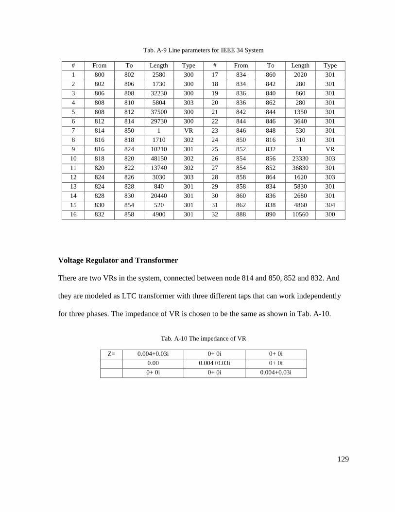
Tab. A-9 Line parameters for IEEE 34 System

# From To Length Type # From To Length Type 1 800 802 2580 300 17 834 860 2020 301 2 802 806 1730 300 18 834 842 280 301 3 806 808 32230 300 19 836 840 860 301 4 808 810 5804 303 20 836 862 280 301 5 808 812 37500 300 21 842 844 1350 301 6 812 814 29730 300 22 844 846 3640 301 7 814 850 1 VR 23 846 848 530 301 8 816 818 1710 302 24 850 816 310 301 9 816 824 10210 301 25 852 832 1 VR

10 818 820 48150 302 26 854 856 23330 303 11 820 822 13740 302 27 854 852 36830 301 12 824 826 3030 303 28 858 864 1620 303 13 824 828 840 301 29 858 834 5830 301 14 828 830 20440 301 30 860 836 2680 301 15 830 854 520 301 31 862 838 4860 304 16 832 858 4900 301 32 888 890 10560 300

Voltage Regulator and Transformer

There are two VRs in the system, connected between node 814 and 850, 852 and 832. And

they are modeled as LTC transformer with three different taps that can work independently

for three phases. The impedance of VR is chosen to be the same as shown in Tab. A-10.

Tab. A-10 The impedance of VR

Z= 0.004+0.03i 0+ 0i 0+ 0i 0.00 0.004+0.03i 0+ 0i 0+ 0i 0+ 0i 0.004+0.03i

129

There are two types of transformer in the original IEEE 34 node system. The rated voltage of

substation transformer is 69kV/24.9kV, and for transformer 832 is 24.9kV/4.16 kV. The

impedances of these two transformers are shown in Tab. A-11.

Tab. A-11 Transformer parameters for IEEE 34 System (a) substation transformer (b) distribution transformer

Tab. A-11 (a)

Z= 2.48+19.84i 0+ 0i 0+ 0i 0.00 2.48+19.84i 0+ 0i 0+ 0i 0+ 0i 2.48+19.84i

Tab. A-11 (b)

Z= 0.057+ 0.1224i 0+ 0i 0+ 0i 0+ 0i 0.057+ 0.1224i 0+ 0i 0+ 0i 0+ 0i 0.057+ 0.1224i

130

Appendix III: Voltage Regulator Control Logic

Start

1s delay at the beginning,Initial tap position is zero

Is Vdiff>half bandwidth?

Yes

0.13s delay

Calculate Error

Check if |Error| >0.05

Yes

0.01s delay, Update the tap position

No

Store the current tap position

No Go to next iteration

Fig. A-1 (a)

131

Start to calculate Error Vdiff>0 Error= Vdiff-half bandwidth

Error= -Vdiff+half bandwidthVdiff<0

Error=0Vdiff=0

Fig. A-1 (b)

Start to adjust tap position Increase tap position by one step

Increase tap position by one step

Tap position unchanged

Error>0.05

Error<-0.05

Else

Fig. A-1 (c)

Fig. A-1 The control logic of the voltage regulator in this thesis

132

an investigation of vvc on freedm systems

Documents