an investigation into stereo algorithms: an emphasis on
TRANSCRIPT

An investigation into stereo algorithms: An emphasison local-matching
Thulani Ndhlovu
Submitted to the Department of Electrical Engineering,University of Cape Town, in fullfillment of the requirements
for the degree of Master of Science in Engineering.March 2011

i
Declaration
I declare that this dissertation is my own work. It is being submitted for the degreeof Master of Science in Engineering at the University of Cape Town. It has not beensubmitted before for any degree or examination at this or any other institution.
...........................Thulani Ndhlovu(Candidate’s Signature)

ii
Acknowledgments
I would like to thank the following people and institutions for their contributiontowards this thesis
• Dr Fred Nicolls and Deon Sabatta for their guidance and help.
• The Council for Scientific and Industrial Reasearch, Mobile Intelligent Au-tonomous Systems unit for their financial assistance.
• My family and friends for their support.

iii
Abstract
Stereo vision attempts to reconstruct the 3D structure of a scene given two im-ages. The main difficulty with stereo vision is the correspondence problem. Local-matching stereo algorithms are an attractive solution to this problem because theyhave a uniform structure and can be paralellized. This makes them applicable inreal-time systems because they can be implemented on graphics processing units(GPUs) and field programmable gate arrays (FPGAs). This thesis closely analyseslocal-matching algorithms and explores two issues.
The first issue is that of using temporal seeding in stereo image sequences. In astereo image sequence, finding feature correspondences is normally done for everyframe without taking temporal information into account. Reusing previous compu-tations can add valuable information. A temporal seeding technique is developedfor reusing computed disparity estimates on features in a stereo image sequence toconstrain the disparity search range. Features are detected on a left image andtheir disparity estimates are computed using a local-matching algorithm. The fea-tures are then tracked to a successive left image of the sequence and by using thepreviously calculated disparity estimates, the disparity search range is constrained.Errors between the local-matching and the temporal seeding algorithms are analysedon a short and long dataset. Results show that although temporal seeding suffersfrom error propagation, a decrease in computational time of approximately 20% isobtained when it is applied on 87 frames of a stereo sequence.
The second issue is that of developing a confidence measure for local-matching stereoalgorithms. A confidence measure is developed and applied to individual disparityestimates in local-matching stereo correspondence algorithms. It aims at identifyingtextureless areas, where most local-matching algorithms fail. The confidence mea-sure works by analyzing the correlation curve produced during the matching process.The measure is tested by developing an easily parallelized local-matching algorithm,and is used to filter out unreliable disparity estimates. Using the Middlebury datasetand the developed evaluation scheme, the results show that the confidence measuresignificantly decreases the disparity estimate errors at a low computational over-head. Furthermore, the confidence measure is used to improve start-up disparitiesin temporal seeding. Results show that the measure does not succeed in filteringout features producing high errors.


Contents
1 Introduction 11.1 Background . . . . . . . . . . . . . . . . . . . . . . . . . . . . . . . . 21.2 Stereo correspondence . . . . . . . . . . . . . . . . . . . . . . . . . . 3
1.2.1 Local-matching stereo algorithms . . . . . . . . . . . . . . . . 31.2.2 Global optimization . . . . . . . . . . . . . . . . . . . . . . . 41.2.3 Dynamic Programming . . . . . . . . . . . . . . . . . . . . . 51.2.4 Cooperative optimization . . . . . . . . . . . . . . . . . . . . 71.2.5 Comparison . . . . . . . . . . . . . . . . . . . . . . . . . . . . 7
1.3 Objectives . . . . . . . . . . . . . . . . . . . . . . . . . . . . . . . . . 91.4 Overview of Thesis . . . . . . . . . . . . . . . . . . . . . . . . . . . . 10
2 Stereo Geometry 112.1 Single view geometry . . . . . . . . . . . . . . . . . . . . . . . . . . . 11
2.1.1 Homogeneous coordinates . . . . . . . . . . . . . . . . . . . . 112.1.2 Pinhole camera model . . . . . . . . . . . . . . . . . . . . . . 112.1.3 Extension of the pinhole camera model . . . . . . . . . . . . . 122.1.4 Camera calibration . . . . . . . . . . . . . . . . . . . . . . . . 13
2.2 Binocular view geometry . . . . . . . . . . . . . . . . . . . . . . . . . 142.2.1 Stereo calibration . . . . . . . . . . . . . . . . . . . . . . . . . 142.2.2 Epipolar geometry . . . . . . . . . . . . . . . . . . . . . . . . 162.2.3 Rectification . . . . . . . . . . . . . . . . . . . . . . . . . . . 172.2.4 Triangulation . . . . . . . . . . . . . . . . . . . . . . . . . . . 19
3 Literature review 213.1 Review of stereo correspondence algorithms . . . . . . . . . . . . . . 21
4 Local-matching stereo algorithms 254.1 Simple local-matching algorithm . . . . . . . . . . . . . . . . . . . . 26
4.1.1 Matching Cost . . . . . . . . . . . . . . . . . . . . . . . . . . 264.1.2 Ordering Constraint . . . . . . . . . . . . . . . . . . . . . . . 274.1.3 Disparity computation . . . . . . . . . . . . . . . . . . . . . . 284.1.4 Cost Aggregation . . . . . . . . . . . . . . . . . . . . . . . . . 284.1.5 Disparity refinement . . . . . . . . . . . . . . . . . . . . . . . 29
4.2 Pseudo-code . . . . . . . . . . . . . . . . . . . . . . . . . . . . . . . . 314.3 Adaptive weights for cost aggregation . . . . . . . . . . . . . . . . . . 31
5 Temporal seeding in stereo image sequences 335.1 Related work . . . . . . . . . . . . . . . . . . . . . . . . . . . . . . . 345.2 Problem statement . . . . . . . . . . . . . . . . . . . . . . . . . . . . 355.3 Feature detection and matching . . . . . . . . . . . . . . . . . . . . . 35

vi Contents
5.3.1 KLT (Kanade-Lucas-Tomasi) . . . . . . . . . . . . . . . . . . 355.4 Stereo correspondence . . . . . . . . . . . . . . . . . . . . . . . . . . 36
5.4.1 Stereo algorithm . . . . . . . . . . . . . . . . . . . . . . . . . 365.5 Temporal seeding . . . . . . . . . . . . . . . . . . . . . . . . . . . . . 37
5.5.1 Assumptions . . . . . . . . . . . . . . . . . . . . . . . . . . . 375.5.2 Seeding . . . . . . . . . . . . . . . . . . . . . . . . . . . . . . 37
5.6 Experiments and results . . . . . . . . . . . . . . . . . . . . . . . . . 385.6.1 Ground truth . . . . . . . . . . . . . . . . . . . . . . . . . . . 385.6.2 Experiments . . . . . . . . . . . . . . . . . . . . . . . . . . . . 38
5.7 Further experiments . . . . . . . . . . . . . . . . . . . . . . . . . . . 41
6 Confidence measure 456.1 Related work . . . . . . . . . . . . . . . . . . . . . . . . . . . . . . . 456.2 Stereo algorithm . . . . . . . . . . . . . . . . . . . . . . . . . . . . . 466.3 Confidence measure for local-matching stereo algorithms . . . . . . . 46
6.3.1 Disparity refinement . . . . . . . . . . . . . . . . . . . . . . . 476.4 Experiments . . . . . . . . . . . . . . . . . . . . . . . . . . . . . . . . 486.5 Confidence measure in temporal seeding . . . . . . . . . . . . . . . . 50
7 Conclusions 557.1 Conclusions . . . . . . . . . . . . . . . . . . . . . . . . . . . . . . . . 55
7.1.1 Temporal seeding . . . . . . . . . . . . . . . . . . . . . . . . . 557.1.2 Confidence measure . . . . . . . . . . . . . . . . . . . . . . . 56
7.2 Future work . . . . . . . . . . . . . . . . . . . . . . . . . . . . . . . . 56
Bibliography 57

List of Figures
1.1 Two images used in stereo-vision with the ground truth disparity map.The images are from the Middlebury dataset [1]. . . . . . . . . . . . 2
1.2 The block diagram of a stereo vision system consisting of five steps:image acquisition, calibration, rectification, stereo correspondenceand triangulation. . . . . . . . . . . . . . . . . . . . . . . . . . . . . . 3
1.3 Stereo images showing the local-matching process. . . . . . . . . . . 41.4 Image of the graph used in graph cuts. . . . . . . . . . . . . . . . . . 61.5 Stereo matching using dynamic programming . . . . . . . . . . . . . 61.6 Comparison of results obtained by SSD, DP and GC on Tsukuba
dataset. . . . . . . . . . . . . . . . . . . . . . . . . . . . . . . . . . . 8
2.1 Pinhole camera geometry. Projection of a 3D point X onto point x
on the image plane using a pinhole camera model. . . . . . . . . . . 122.2 A picture of the checkerboard pattern used for calibration. . . . . . . 142.3 Images showing stages of the calibration process. . . . . . . . . . . . 152.4 Point correspondence geometry. The two cameras are indicated by
their centers C and C′ and image planes. The camera centers, thepoint X, and its images x and x′ all lie on a common plane π. . . . . 16
2.5 Epipolar geometry. The camera baseline intersects each image planeat the epipoles e and e′. Any plane π containing the baseline isan epipolar plane, and intersects the image planes on correspondingepipolar lines l and l′. . . . . . . . . . . . . . . . . . . . . . . . . . . 17
2.6 Image rectification. The two images are calibrated and rectified. Byrectifying the images the scanlines of both images are aligned whichrestricts the correspondence search. . . . . . . . . . . . . . . . . . . . 18
2.7 Triangulation of X using similar triangles. The depth Z is triangu-lated using the disparity d of the two image coordinates of X. . . . . 19
2.8 Depth vs. disparity for f = 1000 (measured in pixels) and B = 12cm.The image shows that for large disparities, the depth resolution is highand decreases as the disparities become smaller. . . . . . . . . . . . . 20
4.1 The ordering constraint violated if features are thin objects close tothe camera. . . . . . . . . . . . . . . . . . . . . . . . . . . . . . . . . 27
4.2 Correlation curve produced by calculating the pixel simmilarity be-tween the pixel of interest and candidate matching pixels. . . . . . . 28
4.3 Results of using the absolute differences as a matching cost for stereocorrespondence. . . . . . . . . . . . . . . . . . . . . . . . . . . . . . . 29
4.4 Disparity maps obtained by varying the support window size. . . . . 304.5 Results produced by using adaptive weights for cost aggregation. . . 32

viii List of Figures
5.1 Features detected in the image. 313 KLT features are detected onthis image. . . . . . . . . . . . . . . . . . . . . . . . . . . . . . . . . . 36
5.2 Correlation curves for a feature point in F at time t and t+ 1. . . . 385.3 Dataset used in the experiments. . . . . . . . . . . . . . . . . . . . . 395.4 Plot of window size versus RMSE for temporal seeding. . . . . . . . 405.5 First stereo image pair of the Microsoft i2i chairs dataset. . . . . . . 415.6 Number of frames versus the number of features in temporal seeding. 425.7 Number of frames versus RMSE in temporal seeding. . . . . . . . . . 43
6.1 Dense disparity map of the Tsukuba image pair using Birchfield andTomasi’s sampling insensitive cost. . . . . . . . . . . . . . . . . . . . 46
6.2 Correlation curve and the basin of convergence. . . . . . . . . . . . . 476.3 Disparity map with disparity estimates of Cd > 2
15 . Estimates whichdo not satisy the condition, Cd > 2
15 are filtered out. . . . . . . . . . 486.4 Number of pixels Np versus Threshold (T ) with a 5× 5 window size
for the Tsukuba image pair. . . . . . . . . . . . . . . . . . . . . . . . 506.5 Threshold T versus RMSE for varying window sizes. . . . . . . . . . 506.6 Number of features detected on the stereo image sequence which have
a chosen confidence. . . . . . . . . . . . . . . . . . . . . . . . . . . . 526.7 RMSE versus the number of frames for different confidence values. . 53

List of Tables
1.1 Table showing the percentage of bad pixels of the SSD, DP and GCalgorithms on the Middlebury dataset. . . . . . . . . . . . . . . . . . 9
1.2 Computation times of the SSD, DP and GC algorithms on the Mid-dlebury dataset. . . . . . . . . . . . . . . . . . . . . . . . . . . . . . . 9
5.1 Table showing the Root Mean Square Error (RMSE) and computa-tional times on 313 KLT features for BT’s stereo algorithm and thetemporal seeding algorithm using chosen stereo parameters. . . . . . 39
6.1 RMSE with a chosen window size, number of disparities, and thresh-old T = 0 for the Middlebury dataset. . . . . . . . . . . . . . . . . . 49
6.2 RMSE for a chosen window size, an empirically selected T value andthe percentage computational overhead for the Middlebury dataset. . 49


Chapter 1
Introduction
Computer vision is the field of study that concerns extracting descriptions of theworld from images or sequences of images. This field is attractive because passiveimaging sensors such as cameras are relatively cheap compared to alternative sensorssuch as laser range finders. We are interested in the stereo vision aspect of computervision.
In stereo vision we attempt to reconstruct the 3D structure of a scene given twoimages. The main difficulty with stereo vision is the correspondence problem statedas follows: given two images of the same scene from slightly different viewpoints,find corresponding pixels and the disparity, the distance by which the pixel in oneview is translated relative to its corresponding pixel in the other view. Solving thecorrespondence problem results in a 2.5D representation of the scene as shown inFigure 1.1. To recover the 3D coordinates, the corresponding pixels are triangu-lated.
The process of retrieving 3D data from stereo cameras may appear simple at first,because as humans we have two eyes and we are able to perceive 3D data natu-rally. It turns out that for a computer this is a complex task, and determiningcorrespondences between pixels is a challenging problem. Some of the challengesare caused by image variations between the two views of the scene. These differ-ences might be caused by occlusions of objects, specular reflections and sensor noise.
A large number of stereo algorithms have been proposed to solve the stereo cor-respondence problem. However, the problem is ill-posed and a satisfying solutionhas not yet been reached [2, 3]. Nevertheless, many algorithms exist and can beuseful depending on the application.
The fact that stereo vision uses cameras, which are passive sensors, makes it anattractive solution to capturing 3D data. While other sensors are available to cap-ture 3D data, cameras are comparatively less expensive and produce a large volumeof information. Applications for stereo vision include mobile robotics where a robotperceives the environment in order to navigate itself while avoiding obstacles [4].In such an application, stereo vision is normally used for Simultaneous Localisationand Mapping (SLAM) [5]. In SLAM the robot builds a map and localises itselfwithin the map while building it. Other applications include augmented reality [6]where virtual objects may be inserted into real world scenes, and human computer-

2 Chapter 1. Introduction
(a) Left image. (b) Right image.
(c) Ground truth disparity map where objectscloser to the camera are represented by thebright color (white) while objects further awayare represented by the dark color (black).
Figure 1.1: Two images used in stereo-vision with the ground truth disparity map.The images are from the Middlebury dataset [1].
interaction [7] where a computer needs to recognize the pose or gesture of a subject.
1.1 Background
The aim of a stereo vision system is to retrieve depth information of a scene fromtwo images which are taken from slightly different viewpoints. Figure 1.2 shows ablock diagram of a stereo vision system. It consists of five main steps: (1) calibrat-ing the cameras; (2) acquiring stereo images; (3) rectifying the stereo images; (4)finding pixel correspondences; and (5) triangulating the pixel correspondences.
The camera calibration stage is two-fold. Firstly, the two cameras are calibratedindependently to find their intrinsic and extrinsic parameters. Secondly, the twocameras are calibrated with each other to find the geometric relationship betweenthem.
After calibrating the cameras, images of the real-world can be acquired. The ac-

1.2. Stereo correspondence 3
Figure 1.2: The block diagram of a stereo vision system consisting of five steps: im-age acquisition, calibration, rectification, stereo correspondence and triangulation.
quisition of stereo images requires the two images to be captured at the same time.This means that the two cameras have to be synchronized.
Image rectification is a pre-processing step for stereo correspondence. This stagemakes use of the calibration between the two cameras and epipolar geometry totransform the images so that their scanlines are aligned. This simplifies the stereocorrespondence search from 2D to 1D.
The stereo correspondence stage is concerned with finding corresponding pixels be-tween the two stereo images. After finding the corresponding pixels, the disparityof a pixel is determined. Stereo correspondence is a challenging problem in stereovision. This problem will be given a fair amount of attention.
The last stage is triangulation. The corresponding pixels in the two stereo im-ages are used to find the depth of the scene points by triangulation. Furthermore,the Euclidean coordinates of the scene points can be determined.
1.2 Stereo correspondence
As mentioned before, stereo correspondence is a challenging problem. Many algo-rithms exist to solve this problem [2]. In this section, different stereo correspondencealgorithms which form building blocks for much more complex algorithms are ex-plained and compared.
1.2.1 Local-matching stereo algorithms
The earliest attempts into solving the stereo correspondence problem involve theuse of local-matching algorithms [8, 9]. These algorithms generally use some kind ofstatistical correlation between colour or intensity patterns in local support windows.By using the local support windows, the image ambiguity is reduced efficiently whilethe discriminative power of the similarity measure is increased. A common local-matching algorithm is the sum of squared differences (SSD) algorithm.

4 Chapter 1. Introduction
The SSD algorithm takes a window of size m × n centered at a pixel of interestin the left image and searches in the right image, along a scanline, for a windowwith similar intensities. This is shown in Figure 1.3.
m
n
(a) Left image.
d
(b) Right image.
Figure 1.3: Stereo images showing the local-matching process.
At each step of the search, the difference E of the two windows is calculated us-ing the equation
E =∑m,n
(IL(m,n)− IR(m,n− d))2, (1.1)
where IL and IR are the intensity values of the left and right images respectivelyand d is the current disparity offset. The pixel in the right image corresponding tothe disparity value with the lowest E is then nominated as the best match for thecurrent pixel in the left image.
In this type of approach finding the correct match can be challenging, especiallyin weakly-textured areas where there is very little information to distinguish onepixel from the next. It has been shown that by breaking down the algorithms andoptimizing the components, they can produce high quality disparity maps [10]. Oneadvantage of these algorithms is that they can be parallelized and implementedon Graphics Processing Units (GPUs) [11] or Field Programmable Gate Arrays(FPGAs) [12] to achieve real-time speeds. This makes these algorithms useful inapplications such as mobile robotics.
1.2.2 Global optimization
Global optimization methods [13, 14, 15, 16] work by defining an energy functionfor the whole image. The problem then is to find a disparity d that minimizes someglobal function. The most commonly used energy function is the Potts model [17],
E(d) = Edata(d) + Esmooth(d). (1.2)

1.2. Stereo correspondence 5
The data term, Edata(d), measures how well the disparity function d agrees withthe input image pair. The smoothness term Esmooth(d) encodes the smoothnessassumptions made by the algorithm. Once the global energy has been defined, avariety of algorithms can be used to find a (local) minimum. One common algorithmis graph cuts (GC).
Using graph cuts, the stereo correspondence problem now becomes that of tryingto find the maximum flow through a 3D graph. G = (V ;E) is defined as a directedgraph, where V is the set of vertices and E is the set of edges. The set of verticesis based on the set of all possible matches and is defined as
V = L ∪ {s, t}, (1.3)
where s is the source and t is the sink. L is defined as
L = {(x, y, d), x ∈ [0, xmax], y ∈ [0, ymax], d ∈ [0, dmax]} , (1.4)
where xmax and ymax correspond to the width and height of the images and dmax
to the range of disparities. The set of edges is defined as
E =
(u, v) ∈ L× L : |u− v| = 1
(s, (x, y, 0)) : x ∈ [0, xmax]
((x, y, dmax), t) : y ∈ [0, ymax]
. (1.5)
Figure 1.4 represents the outline of such a graph. The graph is six-connected exceptat the extremes, s and t, and each vertex has a cost associated with it. Every edgeof the graph has a flow capacity calculated as a function of the costs of the verticesit connects. The capacities limit the flow from the source to the sink.
A cut through the graph separates the set of vertices V into two parts, the setcontaining the source s and the set containing the sink t. The problem now be-comes that of finding the cut through the graph with the highest flow capacity fromthe source to the sink. The capacity of a cut is the sum of the edge capacities thatdefine the cut. The minimum cut through the graph represents the maximum flowfrom the source to the sink. The disparity labels leading to a minimum cut areassigned to the pixels.
1.2.3 Dynamic Programming
Stereo matching through dynamic programming (DP) [18, 19, 20] can be considereda semi-global method. It finds the global minimum for independent scanlines inpolynomial time. The stereo problem in this context becomes that of finding theminimum cost path, or path of least resistance, through a cost matrix such as theone shown in Figure 1.5. This matrix is constructed by calculating the differencesof all the pixels in the reference scanline and all the pixels of the correspondingscanline over a range of disparity levels.

6 Chapter 1. Introduction
Figure 1.4: Image of the graph used in graph cuts.
Figure 1.5: Stereo matching using dynamic programming taken from [2]. The letters(a−k) represent the intensities along each scanline. The uppercase letters representthe path selected through the matrix. M represents a match, L and R representpartially occluded points corresponding to points only visible to the left and rightimages, respectively.
The name dynamic programming comes from a mathematical process through which

1.2. Stereo correspondence 7
a problem is solved by breaking it into smaller pieces. The smaller problems aresolved first and the collection of all the smaller problems is equivalent to the problemas a whole. The process is used to find the minimum cost path through a cost matrixderived from the image scanlines. First the possible paths through the cost matrixare defined using some constraints. The main constraint used in DP is the orderingconstraint [21]. The cost of a point is defined in a similar manner to the cost inEquation 1.2 but instead of the smoothness term Esmooth(d) there is an occlusionterm Eocclusion(d) to penalize occlusions:
E(d) = Edata(d) + Eocclusion(d). (1.6)
The minimum cost to reach a particular point is then calculated and used to calcu-late the minimum cost of reaching the next point of any path that moves throughthe first point.
One advantage of global and semi-global methods is that, to a certain degree, theyare insensitive to weakly-textured areas. In DP the path will not stray far from thedisparities at the edges of the textureless area, because that would increase the costof the path.
1.2.4 Cooperative optimization
Cooperative methods [22, 23] firstly use colour or grayscale information to segmentthe captured images, and then obtain the initial disparity estimate of the scene byusing a known matching algorithm. Finally, a disparity fitting technique is employedto perform the task of disparity refinement for each region. Label-based optimiza-tion is used. Furthermore, the algorithms reduce the number of labels by clusteringregions in the parameter space of the disparity plane before optimization.
These forms of algorithms are amongst the best performing according to the Middle-bury evaluation. However, their main drawback is that they are iterative in nature,making them very slow and inapplicable to real or near real-time systems. Thus,we only discuss them briefly.
1.2.5 Comparison
Figure 1.6 shows the depth maps obtained from the Middlebury Tsukuba datasetfor the three different approaches described above. The implementation comes from[2]. For local-matching algorithms results of the SSD approach are shown, for semi-global matching results from the DP algorithm are shown, and for global matchingresults from the GC optimization algorithm are shown.
The SSD algorithm performs the worst out of the three with most errors occur-ring on the boundaries of the objects, which appear to be bigger than they actuallyare. This problem is due to the design of local-matching algorithms. Approaches

8 Chapter 1. Introduction
exist to address this problem [24, 25] at an extra computation cost. The DP al-gorithm produces better results than SSD but because the scanlines are optimizedindependently, the algorithm suffers from the streaking effect. The algorithm in [26]has been developed to address this problem at extra computational cost. Amongstthe three algorithms, GC performs the best with few errors compared to the othertwo approaches. The advantage of using global reasoning is effectively demonstrated.
(a) Ground truth disparity map. (b) Disparity map produced by using the SSDalgorithm.
(c) Disparity map produced by using the DPalgorithm.
(d) Disparity map produced by using the GCalgorithm.
Figure 1.6: Comparison of results obtained by SSD, DP and GC on Tsukuba dataset.
Table 1.1 shows the values for the percentage of bad pixels produced by the al-gorithms on the Middlebury dataset when using the Middlebury evaluation scheme.The table agrees with the observations of the disparity maps. SSD gives most erro-neous results while GC gives the least erroneous results. DP falls between the twoother algorithms.
Table 1.2 shows the computation times of the different algorithms on the Mid-dlebury dataset. On average, SSD is the fastest followed by DP and GC has theheaviest computational load. This demonstrates that there is a compromise between

1.3. Objectives 9
Table 1.1: Table showing the percentage of bad pixels of the SSD, DP and GCalgorithms on the Middlebury dataset.
SSD DP GC% of bad pixels 15.7 14.2 11.4
quality and speed in stereo correspondence algorithms. A simple algorithm such asSSD produces the most erroneous results at a low computational cost while a morecomplex algorithm such as GC produces fewer errors at a relatively higher compu-tational cost.
Table 1.2: Computation times of the SSD, DP and GC algorithms on the Middleburydataset.
Tsukuba Sawtooth Venus MapTime (seconds)
SSD 1.1 1.5 1.7 0.8DP 1.0 1.8 1.9 0.8GC 23.6 43.8 51.3 22.3
1.3 Objectives
In this study, we firstly aim to understand the different stereo algorithms available.Then we choose to closely analyze local-matching stereo algorithms to explore thefollowing:
1. Temporal seeding in stereo image sequencesIn a stereo image sequence, finding feature correspondences is normally donefor every pair of frames without taking temporal information into account.Current imaging sensors can acquire images at high frequencies resulting insmall movements between consecutive image frames. Since there are smallinter-frame movements, the frame-to-frame disparity estimates do not changesignificantly. We explore using previously computed disparity estimates toseed the matching process of the current stereo image pair.
Most conventional stereo correspondence algorithms contain fixed disparitysearch ranges by assuming the depth range of the scene. This range stays con-stant throughout a stereo image sequence. By decreasing the disparity searchrange the efficiency of the matching process can be improved.

10 Chapter 1. Introduction
2. Confidence measure for local-matching stereo algorithmsLocal-matching stereo algorithms generally fail in textureless regions. Oneway of dealing with these regions is to perform colour segmentation as a pre-processing step [27]. However, this adds a significant overhead on the stereoalgorithm which is undesirable for real-time applications.
A method of assigning a confidence to a disparity estimate for local-matchingalgorithms is explored. This approach is expected to give low confidencesto disparity estimates in textureless regions, where many local-matching algo-rithms fail. While this approach is similar to a number of previously developedconfidence measures [28, 29], in that the confidence of a disparity estimate isa by-product of the matching process, the analysis focuses on the basin ofconvergence (refer to Figure 6.2) of a disparity estimate. Furthermore, highconfidence points are expected to work well in temporal seeding.
1.4 Overview of Thesis
This section provides a brief summary of the work being reported on by outliningthe contents of the rest of the thesis.
In Chapter 2, the geometry of a canonical camera is briefly discussed. A secondcamera is introduced and it is shown how to infer depth information. Epipolar ge-ometry and triangulation are also covered.
In Chapter 3 the literature concerning the stereo correspondence problem is covered.
In Chapter 4 local-matching stereo algorithms are discussed in detail. The algo-rithms are separated into their components and the different design considerationsare discussed.
In Chapter 5 temporal seeding on a stereo image sequence is explored. It is shownhow previously computed disparity maps can be used to aid the matching processin local-matching stereo algorithms.
In Chapter 6 a confidence to a disparity estimate is assigned and used to filterout errors in local-matching stereo algorithms. Furthermore, the confidence mea-sure is used in temporal seeding.
In Chapter 7 the findings are discussed. Possibilities for future research are men-tioned and concluding remarks are made.

Chapter 2
Stereo Geometry
Stereo geometry refers to the geometric relationship between two cameras. In thischapter the objective is to reach a point where depth information can be inferredgiven stereo images. The journey begins by describing how to mathematically repre-sent the geometry of a single ideal camera. A second camera is then introduced andthe relationship between two camera views is described by using epipolar geometry.The process of image rectification is described and used to simplify epipolar geom-etry. The chapter is concluded by describing how to use triangulation to determinedepth information from stereo images.
This chapter forms a basis for this thesis. Terms commonly used in stereo visionand notation used throughout the document are introduced.
2.1 Single view geometry
This section provides a brief summary of the geometry of a single camera.
2.1.1 Homogeneous coordinates
Homogeneous coordinates are useful in computer vision and they form a basisfor the projective geometry used to project a three-dimensional scene onto a two-dimensional plane. A point (x, y) in 2-D space is represented in homogeneous co-ordinates by the triple (kx, ky, k). Given a homogeneous point (kx, ky, k), one cantransform to the original coordinates by dividing by the scalar k. There are two im-portant properties of homogeneous coordinates. Firstly, scalar multiples of a pointrepresent the same point, so (kx, ky, k) is same as the point (x, y, 1) for any non-zerovalue of k. Secondly, points at infinity are represented by the point (x, y, 0), becausewhen transforming the homogeneous coordinates back into the original coordinateswe have to divide by zero.
2.1.2 Pinhole camera model
The process of mathematically representing a physical system usually begins withconstructing an ideal mathematical model. The model is then extended by includingdeviations which occur in the real world. The most commonly used camera modelis the pinhole camera. This model describes the relationship of a 3D point in spaceto its 2D projection on the image plane.

12 Chapter 2. Stereo Geometry
pf
C
Y
Z
f Y / Z
y
Y
x
X
x
p
image planecameracentre
Z
principal axis
C
X
Figure 2.1: Pinhole camera geometry. Projection of a 3D point X onto point x onthe image plane using a pinhole camera model.
The model assumes that every light ray entering the camera passes through a singlepoint called the camera center, C. The canonical camera center is taken as theorigin of the Euclidean coordinate system. The image is produced as the light raysintersect the image plane which lies at a specific distance f from the camera center.This distance f is known as the focal length of the camera. A point X = (X,Y, Z)T
in R3 is projected onto a point x = (x, y)T on the image plane in R2 where theray emanating from X and passing through the camera center intersects the imageplane. Referring to Figure 2.1 it can be shown using similar triangles that
(X,Y, Z)T 7→(fX
Z,fY
Z, f
)T
. (2.1)
If the world and image points are represented by homogeneous vectors, the projec-tion can be expressed as a linear mapping and can be written as
X
Y
Z
1
7→
fX
fY
Z
=
f 0 0 0
0 f 0 0
0 0 1 0
X
Y
Z
1
. (2.2)
Now, if the world point X is represented as a homogenous 4-vector (X,Y, Z, 1)T andthe image point x is represented as a 3-vector, Equation 2.2 can be written as
x = PX, (2.3)
where P is a 3× 4 homogenous camera projection matrix.
2.1.3 Extension of the pinhole camera model
In order to better model a real camera, the pinhole camera model is extended [30].These extensions include the following.
1. Principal point offsetThis takes into account the fact that the origin of the camera coordinatesmight not lie on the camera center.

2.1. Single view geometry 13
2. Distortion correctionA pinhole camera is not ideal for making images because it does not gatherenough light for rapid exposure. In order to gather more light, cameras uselenses. The disadvantage of using lenses is that they introduce distortions.The two main lens distortions are radial distortions and tangential distortions.These distortions are modelled and corrected on the images.
3. Pixel shapeThe pinhole camera model assumes that the image coordinates are Euclideancoordinates having equal scales on both vertical and horizontal directions. Inthe case of CCD cameras, there is the additional possibility of having non-square pixels. If image coordinates are measured in pixels, then this has theeffect of introducing unequal scale factors in each direction.
4. Extrinsic parametersExtrinsic parameters are the external parameters, which are the position andorientation of the camera in the world coordinates. The camera and worldcoordinates are related by a Euclidean transformation which gives a rotationand translation.
After extending the pinhole camera model, Equation 2.3 now becomes
x = PX = K[R|t]X, (2.4)
where P = K[R|t]. The matrix K contains the intrinsic parameters of the cameraand is called the intrinsic parameter matrix or the calibration matrix. R and t arethe rotation and translation that relate the world coordinate frame to the cameracoordinate frame.
2.1.4 Camera calibration
Camera calibration is used to estimate P . One of the most used methods for cam-era calibration is by Zhang [31]. This process uses a checkerboard pattern of knowndimensions, as shown in Figure 2.2. Many calibration toolboxes exist that have thenecessary steps for calibration built in. Some of the most common ones includeOpenCV [32] and the Bouguet camera calibration toolbox [33].
To calibrate a camera, multiple views of the calibration object are taken at dif-ferent orientations and angles as shown in Figure 2.3(a). The corners of the patternare then detected using a corner detector such as the Harris corner detector [34] andtheir estimated locations are refined to sub-pixel accuracy. Figure 2.3(b) shows atypical result of the corner detection process.
An advantage of this pattern is that the corners of the checkerboard can be de-tected very accurately up to sub-pixel accuracy. Furthermore, the corners form aregular grid in a matrix form which means that errors in the detection of the corners

14 Chapter 2. Stereo Geometry
Figure 2.2: A picture of the checkerboard pattern used for calibration.
can be resolved by enforcing the grid shape. Also, accurate world coordinates areeasily measured and specified for this pattern.
2.2 Binocular view geometry
A second camera is introduced to complete a stereo vision setup. This section detailstwo-camera geometry necessary for stereo vision.
2.2.1 Stereo calibration
A second camera is now introduced in order to move a step closer to achieving themain objective namely inferring depth information from two cameras. Introducinga second camera arbitrarily would be of no use. For the second camera to be useful,one needs to know the spatial relationship between the two cameras. This meansthat the two cameras have to be calibrated to each other. This process is calledstereo calibration [33]. Stereo calibration works in a similar way to single-cameracalibration except that now there are two cameras. In stereo camera calibrationwe seek a single rotation matrix Rs and a translation vector Ts that relate the twocameras.
For any given 3D point X in world coordinates, single-camera calibration is used tomap the point into the two camera coordinates
x = R1X+ T1
andx′ = R2X+ T2.

2.2. Binocular view geometry 15
Calibration images
(a) Multiple images taken from different viewpoints for calibrationusing the Bouguet camera calibration toolbox.
OdX
dY
Xc (in camera frame)
Yc
(in c
amer
a fr
ame)
Extracted corners
100 200 300 400 500 600
50
100
150
200
250
300
350
400
450
(b) Image showing the checkerboard corners extracted onthe first image in (a) using the Bouguet camera calibrationtoolbox.
Figure 2.3: Images showing stages of the calibration process.
The two views of X are then related by
x = RTs (x
′ − Ts). (2.5)
The three equations mentioned above can now be used to solve for the rotation andtranslation separately as
Rs = R2(R1)T , Ts = T2 −RsT1. (2.6)
The stereo camera calibration process requires one to capture images of the samecheckerboard with both cameras at the same time. Furthermore, to relate the point

16 Chapter 2. Stereo Geometry
correspondences from the two cameras, the checkerboard has to be clearly visible inboth images.
2.2.2 Epipolar geometry
The epipolar geometry [30] between two views is essentially the geometry of theintersection of the image plane with a pencil of planes having the baseline as theaxis, where the baseline is the line joining the camera centers.
Suppose a point X in 3-space is imaged in x in the first camera view and x′ inthe second. We seek to find the relationship between the corresponding points x
and x′. As shown in Figure 2.4, the image points x and x′, the space point X, andthe camera centers C and C′, are all coplanar. Denote this plane by π. The raysback-projected from x and x′ intersect at X and the rays are coplanar, lying on π.It is this latter property that is most significant in searching for a correspondence.
C C /
π
x x
X
epipolar plane
/
Figure 2.4: Point correspondence geometry. The two cameras are indicated by theircenters C and C′ and image planes. The camera centers, the point X, and its imagesx and x′ all lie on a common plane π.
Suppose now only x is known and we ask how the corresponding point x′ is con-strained. The plane π is determined by the baseline and the ray defined by x, asshown in Figure 2.5. The ray corresponding to the (unknown) point x′ lies in π,hence the point x′ lies on the line of intersection l′ of π with the second imageplane. This line l′ is the image in the second view of the ray back-projected fromx. It is the epipolar line corresponding to x′. In terms of a stereo correspondencealgorithm the benefit is that a search for a point corresponding to x need not coverthe entire image plane, but can be restricted to the line l′. It turns out that one can

2.2. Binocular view geometry 17
l
e e
l
π
baseline
/
/
Figure 2.5: Epipolar geometry. The camera baseline intersects each image plane atthe epipoles e and e′. Any plane π containing the baseline is an epipolar plane, andintersects the image planes on corresponding epipolar lines l and l′.
further simplify the correspondence search using image rectification. This processis described next.
2.2.3 Rectification
Given a pair of stereo images, rectification [33] determines a geometric transforma-tion of each image plane such that pairs of conjugate epipolar lines become collinearand parallel to one of the image axes (usually the horizontal axis). Effectively thismeans that we have to define a new rotation Rn and a new intrinsic parametermatrix Kn. The rectified images can be thought of as acquired by a new stereo rig,obtained by rotating the original cameras. The important advantage of rectificationis that computing stereo correspondences is made simpler because the search needonly be done along the horizontal lines of the rectified images.
If P1 and P2 are the camera matrices corresponding to the two images, the newintrinsic parameters can be chosen to be
Kn =(K1 +K2)
2. (2.7)
The objective is to have the two images coplanar, meaning that the Z axis of thenew orientation Rn has to be perpendicular to the baseline (the line joining C andC′). This does not ensure that the image scan lines are aligned. For the alignment,the scan lines need to be parallel to the baseline. The first unit vector u1 is chosento be along the baseline. This unit vector corresponds to the X axis of the neworientation and is expressed as
u1 =(C−C′)
||(C−C′)||. (2.8)

18 Chapter 2. Stereo Geometry
In order to define the Y axis the unit vector of the principal ray of the old image,n is used. The Y axis has to be perpendicular to u1, therefore
u2 = n× u1. (2.9)
The last unit vector, u3, corresponding to the Z axis has to be perpendicular toboth u1 and u2, so
u3 = u1 × u2. (2.10)
Now the new rotation can be written as
Rn =
uT1
uT2
uT3
(2.11)
The images may be remapped by defining the transformations S1 and S2 as
S1 = MnM−11 , S2 = MnM
−12 (2.12)
where Mn = KnRn and Mi = KiRi for i = 1, 2. The image points x and x′ of theoriginal images can now be mapped to the rectified image points xrect and x′
rect asfollows:
xrect = S1x, x′rect = S2x. (2.13)
The effect of this mapping can be illustrated in Figure 2.6, where the image scanlinesare aligned.
Figure 2.6: Image rectification. The two images are calibrated and rectified. Byrectifying the images the scanlines of both images are aligned which restricts thecorrespondence search.

2.2. Binocular view geometry 19
2.2.4 Triangulation
At this point, enough has been described to be able to find the 3D coordinate of apoint given undistorted and rectified stereo images. This is done by using triangu-lation. It is assumed that the image coordinates x and x′ of the feature coordinateX in the left and right images respectively are known. Then X can be calculatedby using similar triangles as follows: If x = (u, v), where u and v are the row andcolumn of the image, and x′ = (u′, v′) are the image coordinates of the left and rightimages respectively, then the disparity d is defined as d = v− v′. Given the baselineB and the focal length f of the left camera, the depth Z of X can be determinedby using similar triangles as illustrated in Figure 2.7 as
Figure 2.7: Triangulation of X using similar triangles. The depth Z is triangulatedusing the disparity d of the two image coordinates of X.
B − d
Z − f=
B
Z, (2.14)
Z =fB
d.
The depth of a point is inversely proportional to the disparity. In order to visualizethis relationship one can plot the disparity versus the depth as shown in Figure 2.8.
The figure illustrates that for small values of d, the estimates of the depth based ond become more inaccurate. This point is important to note as the work progresses.Next, one needs to find the X and Y coordinates of the world point X. Usingthe left image of the stereo camera pair, similar triangles can be used to find X as

20 Chapter 2. Stereo Geometry
0 5 10 15 20 25 30 35 40 45 500
20
40
60
80
100
120
Disparity
Dep
th (
cm)
Figure 2.8: Depth vs. disparity for f = 1000 (measured in pixels) and B = 12cm.The image shows that for large disparities, the depth resolution is high and decreasesas the disparities become smaller.
follows:X =
(u− pu)
fZ (2.15)
where pu is the vertical offset of the principal point. Equation 2.15 can be writtenin terms of B and d by substituting for Z as follows:
X =(u− pu)
f
fB
d=
(u− pu)B
d. (2.16)
Similarly,
Y =(v − pv)B
d, (2.17)
where pv is the horizontal offset of the principal point. Homogeneous coordinatescan be used to neatly encapsulate the whole process of triangulation. The matrixQ can be defined such that
WX
WY
WZ
W
= Q
u
v
d
1
, (2.18)
with
Q =
1 0 0 −pu0 1 0 −pv0 0 0 f
0 0 1B 0
. (2.19)
Now one needs to find corresponding pixels in a stereo image pair. This is calledthe stereo correspondence problem and is described in the next chapter.

Chapter 3
Literature review
Stereo vision is one of the most actively researched fields in computer vision. A largenumber of stereo correspondence algorithms have been developed. In order to gaugeprogress in the area, Schartein et al. [2] wrote a paper which provides an update onthe state of the art in dense two frame stereo correspondence algorithms under knowncamera geometry. The algorithms produce dense disparity maps which are usefulin a number of applications including view synthesis, robot navigation, image-basedrendering and tele-presence. For researchers in stereo vision one of the most usefuloutputs of the paper is a quantitative testbed for stereo correspondence algorithmsavailable, from vision.middlebury.edu/stereo. The testbed allows an on-lineevaluation of developed stereo correspondence algorithms and rates the algorithmsaccording to their depth map quality relative to the ground truth. Because ofthe quantitative on-line evaluations the testbed is widely used in the stereo visioncommunity. This section reviews stereo correspondence algorithms mostly whichhave received attention in the Middlebury evaluation [1].
3.1 Review of stereo correspondence algorithms
Top-performing stereo correspondence algorithms make use of colour segmentationtechniques. The mean-shift [35] algorithm is popular for performing colour segmen-tation. Currently, the best performing algorithm in the Middlebury evaluation pageis based on inter-regional cooperative optimization [22]. The algorithm firstly seg-ments the images into homogeneous regions. Secondly, a local-matching algorithm isused to compute the initial disparity estimate. Thirdly, a voting-based plane fittingtechnique is applied to obtain the parameters of a disparity plane corresponding toeach image region. Finally, the disparity plane parameters of all regions are iter-atively optimized by an inter-regional cooperative optimization procedure until areasonable disparity map is obtained. The algorithm in [23] is similar to [22] butinstead of using inter-regional optimization, it uses belief propagation to determinethe optimal plane parameters. The iterative nature of this algorithm makes it veryslow and thus not suitable for real-time implementations.
A slightly different approach to solving the stereo correspondence problem can befound in [36]. Pixels are classified as either stable, unstable or occluded. Occludedpixels are those which fail the left-right consistency check [37, 38]. The distinctive-ness of the correlation measure peak is then used to classify the pixels which passedthe left-right consistency check into stable and unstable pixels. Information from

22 Chapter 3. Literature review
the stable pixels is then propagated to the unstable and occluded pixels by usingcolour segmentation and plane fitting. Hierarchical belief propagation in a globalenergy minimization framework is then used to iteratively improve the plane fittingresults. Instead of classifying pixels as in [36], [39] uses an outlier confidence modelto measure how likely a pixel is occluded. Because there is no direct labelling, themodel has more tolerance for errors produced in the occlusion detection process.The model then uses a reliable colour refinement scheme to locally infer the possibledisparity values for the outlier pixels. Belief propagation is used to minimize theenergy function.
Segmentation-based stereo correspondence algorithms work well in textureless re-gions because they assume that depth varies smoothly within regions of homoge-neous colour, and that depth discontinuities coincide with depth boundaries. Thealgorithm in [40] takes into account the drawback of this assumption: depth discon-tinuities may not lie along colour segmentation boundaries, resulting in segmentsthat span depth discontinuities. In order to overcome this effect, the algorithm in[40] jointly estimates image segmentation, depth, and matting/depth informationfor mixed pixels, which span two objects at different depths. An over-segmentationapproach is used to represent the scene as a collection of fronto-parallel planar seg-ments. The segments are then characterized by their depth, 2D shape and colour.These parameters are jointly estimated by alternating the update of segment shapesand depths. The segment shapes are updated using a generative model that ac-counts for mixed pixels at the segment boundary as well as the depth and shapeprobabilities. Segment depths are updated by defining a pairwise Markov randomfield and belief propagation is used to minimize the energy.
In [41], an explicit treatment of occlusions is carried out. The visibility constraint,which requires that an occluded pixel must have no match on the other image anda non-occluded pixel must have at least one match, is exploited. This results ina symmetric stereo model that can handle occlusions. The visibility constraint isembedded in an energy minimization framework. The energy is minimized withan iterative optimization algorithm that uses belief propagation. In [42], a nearreal-time stereo correspondence algorithm which explicitly deals with texturelessregions is developed. Instead of having strong planarity constraints in the envi-ronment, which tend to force non-planar objects onto planes, the algorithm uses acompromise approach. Depth estimates are preferred while in textureless regions,the estimates can be replaced with planes. A near real-time colour segmentationalgorithm is used and planes are fitted in textureless segments. The planes arerefined using consistency constraints. Loopy belief propagation is used to correctlocal errors and improve the algorithm. The algorithm in [43] uses a window-basedalgorithm to obtain initial depth estimates. Instead of halting the process afterthe initial depth estimation, the process is taken one step further using a techniquecalled disparity calibration. For disparity calibration, an appropriate calibrationwindow is selected for each pixel using colour similarity and geometric proximity.

3.1. Review of stereo correspondence algorithms 23
By using these calibration windows, a local disparity calibration method is designedto acquire accurate disparity estimates.
In [44], an extension of semi-global matching is used to solve stereo correspondence ina structured environment. In order to handle untextured areas, intensity consistentdisparity selection is proposed. Holes caused by filters are filled in by discontinuitypreserving interpolation. One of the main advantages of this algorithm is its lowcomplexity and runtime. The algorithm in [45] is based on scanline optimization(SO). The algorithm embodies a function based on variable support. Low-texturedregions are handled by the SO framework and the variable support helps to preserveaccuracy along depth borders. A refinement step based on a technique that exploitssymmetrically the relationship between occlusions and depth discontinuities on thedisparity maps obtained, assuming alternatively as reference the left and the rightimage, allows for accurately locating borders.
A similarity measure called the Distinctive Similarity Measure (DSM) is proposed in[46]. The DSM resolves the point ambiguity based on the idea that the distinctive-ness, not the interest, is the appropriate criterion under the point ambiguity. Thedistinctiveness of a point is related to the probability of a mismatch. Also, the dis-similarity between image points is used since it is related to the probability of a goodmatch. The algorithm in [10] uses a local algorithm based on adaptive weights forcost aggregation. The algorithm includes information obtained from a segmentationprocess in order to improve aggregation. The algorithm in [47] combines the strengthof the region-based approach and the 2D DP optimization framework. Instead ofoptimizing a global energy function defined on a 2D pixel-tree structure using DP,a region-tree built on over-segmented image regions is used. The resulting disparitymaps do not contain any streaking problems as is common in SO algorithms becauseof the tree structure.
The algorithm in [48] is a local-matching algorithm which uses varying supportweights for cost aggregation. The support weight in a given support window isbased on colour similarity and geometric proximity to reduce the image ambiguity.The algorithm produces surprisingly good results for a local-matching algorithm.The algorithm in [49] solves the stereo correspondence problem by formulating theproblem as a large scale linear programming problem. The match cost function isapproximated by a piecewise linear convex function. The resulting problem is solvedusing an interior point method and the associated Newton steps involve matricesthat reflect the structure of the underlying pixel grid. The algorithm in [50] aims toimprove sub-pixel accuracy in low-texture regions. The algorithm preserves depthdiscontinuities and enforces smoothness on a sub-pixel level. A stereo constraintcalled the gravitational constraint is presented. The constraint assumes sorted dis-parity values in a vertical direction and guides global algorithms to reduce falsematches, especially in low-texture regions.

24 Chapter 3. Literature review
The algorithm in [51] is a semi-global algorithm which uses mutual informationfor pixel-wise matching. The calculation of mutual information is performed hierar-chically. A global cost calculation is approximated and can be performed at a timethat is linear in the number of pixels. The algorithm in [52] uses fast converginghierarchical belief propagation to achieve a real-time stereo correspondence algo-rithm on a graphics processing unit (GPU). A novel approach is used to adaptivelyupdate pixel costs since belief propagation is linear in the number of iterations,making it unfeasible for practical applications. The algorithm in [53] is a two-steplocal stereo correspondence algorithm, initial matching and disparity estimation,which employs segmentation cues. The initial matching uses a raw matching costwith the contrast context histogram descriptor and two-pass cost aggregation withsegmentation-based adaptive support weight. The disparity computation consists oftwo parts: narrow occlusion handling and multi-directional weighted least-squaresfitting for the broad or large occlusion areas.
A near real-time local stereo correspondence algorithm is developed in [27] basedon segmentation. The algorithm uses effective cost aggregation and finds a compro-mise between cost aggregation and computational time. The algorithm in [54] is alocal stereo correspondence algorithm which uses the anisotropic local-polynomialapproximation-intersection of confidence intervals technique in order to define anappropriate window size. The method performs the entire disparity estimation andrefinement within the local high-confidence voting framework. The algorithm in [55]uses a combination of binocular and monocular cues for initial match candidates.The matching candidates are then embedded in disparity space, where perceptualorganization takes place in 3D neighbourhoods. The assumption is that correctmatches produce salient, coherent surfaces, while wrong ones do not. Matchingcandidates that are consistent with the surfaces are kept and grouped into smoothlayers. The projections of the refined surfaces on both images are used to obtaindisparity hypotheses for unmatched pixels. The final disparities are selected aftera second tensor voting stage, during which information is propagated from morereliable pixels to less reliable ones.
The algorithm in [56] is a real-time DP based algorithm on a GPU. The algorithmreduces the typical streaking artifacts by aggregating the per-pixel matching cost inthe vertical direction. The algorithm in [57] uses DP in a tree structure instead ofon the individual scanlines. The nodes on the tree represent image pixels, but onlythe most important edges of the 4-connected neighbourhood system are included.The algorithm becomes a global optimization method because a disparity estimateat one pixel depends on the estimates at all other pixels.

Chapter 4
Local-matching stereo algorithms
The aim of stereo correspondence is to find corresponding pixels between two imagesof the same scene taken from slightly different viewpoints. This means that for apixel in the left image, every pixel in the right image can be scanned to find which onecorresponds. This would be very computationally expensive. Recalling from Section2.2.3, the search space for finding pixel correspondences can be significantly reducedby calibrating and rectifying the images. This simplifies the stereo correspondenceproblem significantly. The problem can now be phrased as: given two images of thesame scene taken from slightly different viewpoints, for a pixel in the left image, finda corresponding pixel in the right image along the same scanline and the distanceby which the pixel in the left image is translated relative to its corresponding pixelin the right image. Mathematically, if x = (u, v) is the left image pixel coordinatewhere u is the image row/scanline and v is the image column and x′ = (u′, v′), isthe right image pixel coordinate, then the correspondence problem can be writtenas:
u = u′, v = v′ − d, (4.1)
where d is the disparity. If we compute d for every pixel in the left image, a densedisparity map is obtained.
The earliest attempts into solving the stereo correspondence problem involve theuse of local-matching algorithms [8, 9]. These algorithms generally use some kind ofstatistical correlation between colour or intensity patterns in local support windows.By using the local support windows, the image ambiguity is reduced efficiently whilethe discriminative power of the similarity measure is increased.
Generally, stereo correspondence algorithms can be broken down into components.These components allow us to separate the different design considerations of a par-ticular algorithm. By separating the algorithms into their components, they can beevaluated thoroughly and the inner workings can be easily understood. The foursteps generally performed by a stereo correspondence algorithm are:
• Matching cost computationA matching cost is defined and used to measure pixel similarity.
• Cost (support) aggregationA support region is defined to spatially aggregate the matching cost.
26 Chapter 4. Local-matching stereo algorithms
• Disparity computation / optimizationThe best disparity hypothesis for each pixel is defined to minimize a costfunction.
• Disparity refinementThe disparity estimates are post-processed to remove outliers and/or performsub-pixel estimation.
A particular algorithm might perform all four steps or a subset of the steps. Thesequence in which they are applied depends on the algorithm. Our interest lies inlocal-matching algorithms that perform all the above-mentioned steps.
In this chapter a basic local-matching stereo algorithm is described by decompos-ing it into the different steps described above. It is then shown that by breakingdown the algorithm we can look at the different design considerations and improveit. The improvement is demonstrated by implementing a state-of-the-art variant oflocal-matching algorithms.
4.1 Simple local-matching algorithm
A simple local-matching algorithm is implemented. The algorithm is broken downinto its components and the different design considerations for the algorithm arecovered.
4.1.1 Matching Cost
In order to find corresponding pixels we need some way of quantifying how similarthey are. To achieve this a matching cost e(x,x′) is defined, where x and x′ arethe pixel locations in the left and right images respectively. By using the intensityvalues at the specific image locations I(.), a matching cost can be defined using theabsolute differences of the pixel intensities as follows:
e(x,x′) = |IL(x)− IR(x′)| (4.2)
where IL(.) and IR(.) represent the intensity at the specific image locations in theleft and right images respectively.
Pixels that are similar will give a low score and ones that are different will givea high score. An extension of the above mentioned matching cost would be Birch-field and Tomasi’s sampling insensitive matching cost [58]. The reader is referred to[59] for a comprehensive study on the performance of matching costs under differentradiometric changes of the input images. Since now there is a way of determiningthe similarity of pixels, the only part left is the process of searching and choosingthe corresponding pixels.

4.1. Simple local-matching algorithm 27
4.1.2 Ordering Constraint
Recalling that the images are calibrated and rectified, the search for correspondingpixels is limited to a single scanline. In order to find correspondences, a pixel inthe left scanline compared to every pixel in the corresponding scanline of the rightimage. It turns out that the search for a corresponding pixel can be reduced byusing an ordering constraint [21].
Considering the two-camera geometry, the ordering constraint can be phrased asfollows: pixels A and B are on the left image and their matches on the right imageare A′ and B′ respectively. If pixel A is on the left of pixel B in the left image,A′ has to be to the left of B′ in the right image. This constraint does not alwayshold: it is violated by thin objects which are close to the camera as demonstratedin Figure 4.1. However, it can be assumed that most objects in the scene are large.The ordering constraint restricts the search for correspondence of a pixel in the leftimage scanline to be to the left of the same pixel in the right image scanline.
Figure 4.1: The ordering constraint violated if features are thin objects close to thecamera.

28 Chapter 4. Local-matching stereo algorithms
4.1.3 Disparity computation
The ordering constraint allows to restrict the correspondence search to a certaindirection. The search can be further reduced by choosing the disparity range tobe d ∈ [dmin, dmax]. Using Equation 4.2 and the ordering constraint, the matchingcosts between the pixel of interest in the left image and the candidate pixels in theright image can be computed. The computation produces a correlation curve asillustrated in Figure 4.2.
0 2 4 6 8 10 12 14 16 18 200
200
400
600
800
1000
1200
1400
1600
Disparity
SA
D
Figure 4.2: Correlation curve produced by calculating the pixel simmilarity betweenthe pixel of interest and candidate matching pixels.
The disparity of the pixel is then selected using a Winner-Takes-All (WTA) methodwithout considering global reasoning as
d = argmin(e(x,x′(d))) = argmin(|IL(u, v)− IR(u′, v′ − d)|). (4.3)
This algorithm gives a disparity map as shown in Figure 4.3.
Although the disparity map in Figure 4.3 is very detailed, it suffers from noise.This is due to the fact that the similarity measure is done pixelwise. To reduce thisnoise one can support the pixels of interest with their neighbouring pixels as shownin the next section.
4.1.4 Cost Aggregation
Using the raw matching cost gives noisy results as shown in Figure 4.3. In order tocombat this problem, a support region is defined to spatially aggregate the matchingcost. A number of aggregation strategies exist [60]. The matching cost can beaggregated by using an n×n window centered at the pixel of interest. Then Equation4.2 becomes
E(x,x′) =∑
xa∈NL,x′a∈NR
|IL(x− xa)− IR(x′ − x′
a)|. (4.4)

4.1. Simple local-matching algorithm 29
(a) Ground truth disparity map. (b) Disparity map produced by using absolutedifferences as a matching cost.
Figure 4.3: Results of using the absolute differences as a matching cost for stereocorrespondence.
where NL and NR represent the support windows centered on pixels x and x′ re-spectively. xa and x′
a are the pixels within NL and NR respectively. Aggregationof this form assumes a constant disparity across the support window. Figure 4.4shows the resultant disparity maps obtained while varying the support window size.
It is observed that increasing the window size reduces the noise in the disparitymaps. Furthermore, the resolution of the disparity map is decreased. Because everypixel of interest has a support window associated with it, the computational time ofthe disparity map is increased. An artifact called the fattening-effect is introducedat the object boundaries. Choosing the optimal window size becomes an importantconsideration in the design of a stereo algorithm. There have been several studiesinto addressing the choice of window size [25].
Three observations can be made from the resulting disparity maps. Firstly, local-matching stereo algorithms fail in weakly-textured regions because there is notenough information to reliably match the pixels in that region. Secondly, if a pixelis occluded, visible in one view and not visible in the other view, the algorithmwill give incorrect results because it does not penalize these occurrences. Thirdly,because the disparities are calculated as discrete values, the algorithm suffers fromthe discretization effect [2]. The next section describes how some of these problemscan be addressed.
4.1.5 Disparity refinement
In this section, some of the post-processing steps used in stereo vision are discussed.

30 Chapter 4. Local-matching stereo algorithms
(a) Ground truth disparity map (b) Disparity map produced by using the sumof absolute differences with a 3 × 3 windowsize.
(c) Disparity map produced by using the sumof absolute differences with a 9 × 9 windowsize.
(d) Disparity map produced by using the sumof absolute differences with a 15× 15 windowsize.
Figure 4.4: Disparity maps obtained by varying the support window size.
4.1.5.1 Left-right consistency check
The left-right consistency check [37, 38, 61, 62] is used to detect inconsistencies inthe matching process. The check works by reversing the roles of the left and rightimages. Firstly, the matching pixel of the left image in the right image is determined.Then the roles of the images are reversed and there is a check if the right imagepixel matches the left image pixel. This check is very useful especially when a pixelis occluded.
4.1.5.2 Sub-pixel refinement
The disparity computation gives discrete disparity values. To remove the dis-cretization effects, one can perform sub-pixel estimation based on quadratic poly-nomial interpolation [63]. dsub is approximated between three discrete variables,f(i) = E(x,x′ − d), f(i+1) = E(x,x′ − (d+1)) and f(i− 1) = E(x,x′ − (d− 1)) as
dsub = d−{
f(i+ 1)− f(i− 1)
2(f(i+ 1) + f(i− 1)− 2f(i)
)}. (4.5)

4.2. Pseudo-code 31
4.2 Pseudo-code
The different design considerations of a local-matching stereo algorithm have beencovered. The algorithms can be summarized in pseudo-code shown in Algorithm 1.
Algorithm 1 Stereo algorithmINPUT: Stereo images, window size, disparity range.OUTPUT: Disparity map.
for each pixel in the left frame doset support region around the pixel (left frame)set search window in the right framefor each pixel in the search window (right frame) do
set correlation window around the pixelcorrelate support region with correlation window
find best matchcalculate disparityrefine disparity
4.3 Adaptive weights for cost aggregation
The algorithm implemented is found in [10]. For a matching cost the algorithm usestruncated absolute differences. The cost is expressed as
e(x,x′) = min(|IL(x)− IR(x′)|, T ), (4.6)
where T is the truncation value that controls the limit of the matching cost. Theintensity values used in this algorithm are based on the Lab color space which closelyrepresents the human visual system. The main contribution of the algorithm is in theaggregation step. Similar to the simple matching algorithm, a square window is usedfor aggregation but with some additions. The approach taken in this algorithm isbased on the observation that pixels in a support region are not equally importantfor support aggregation. Every pixel within a window is given a support weightbased on the gesalt grouping [64, 65]:
w(p, q) = f(∆cpq,∆gpq), (4.7)
where pixel p is the center pixel of the window which is at position (u, v) according tothe previous description. Pixel q is a pixel neighbour of p within the support window.∆cpq and ∆gpq represent the colour difference and spatial difference between pixelp and q. By regarding ∆cpq and ∆gpq as independent events, f(∆cpq,∆gpq) can bewritten as
f(∆cpq,∆gpq) = fs(∆cpq)fp(∆gpq), (4.8)

32 Chapter 4. Local-matching stereo algorithms
(a) Ground truth disparity map. (b) Disparity map produced using adaptiveweights for cost aggregation.
Figure 4.5: Results produced by using adaptive weights for cost aggregation.
where fs(∆cpq) and fp(∆gpq) represent the strength of grouping by similarity andproximity. These groupings are modelled as
fs(∆cpq) = exp
(−∆cpq
γc
)(4.9)
andfp(∆gpq) = exp
(−∆gpq
γp
), (4.10)
where ∆cpq represents the Euclidean distance between two colors, cp = [Lp, ap, bp]
and cq = [Lq, aq, bq]. ∆gpq is the Euclidean distance between p and q in the imagedomain. γc is a factor used in the strength of grouping by similarity and γp isthe radius of the window size. The support weight based on the strength of thegroupings then becomes
w(p, q) = exp
(−(∆cpqγc
+∆gpqγp
)). (4.11)
Using Equation 4.11, the dissimilarity between pixels becomes
E(x,x′) =
∑q∈Np,q̄d∈Np̄d
w(p, q)w(p̄, q̄)e(q, q̄d)∑q∈Np,q̄d∈Np̄d
w(p, q)w(p̄, q̄). (4.12)
The disparity computation used is the same as in Equation 4.3. The results of theextensions to the simple local-matching stereo algorithm are shown in Figure 4.5.

Chapter 5
Temporal seeding in stereo imagesequences
The previous chapter dealt with obtaining a dense disparity map from static images.In this chapter, the temporal domain of a stereo image sequence is explored. In astereo image sequence, finding feature correspondences is normally done for everypair of frames without taking temporal information into account. Current imagingsensors can acquire images at high frequencies resulting in small movements be-tween consecutive image frames. Since there are small inter-frame movements, theframe-to-frame disparity estimates do not change significantly. We explore usingpreviously computed disparity estimates to seed the matching process of the cur-rent stereo image pair.
Most conventional stereo correspondence algorithms contain fixed disparity searchranges by assuming the depth range of the scene as in Equation 4.3. This rangestays constant throughout a stereo image sequence. By decreasing the disparitysearch range the efficiency of the matching process can be improved. This can beseen in [66], where the probability of an incorrect stereo match is given by:
P T ∝ P a + P b + P c,
where P a is the probability of mismatching a pair of features when neither featurehas its correct match detected in another image, P b is the probability of mismatchwhen one feature has had its correct match detected, and P c is the probability ofmismatch when both features have had their correct matches found in the otherimage. The probabilities, P a, P b and P c are all proportional to the mean num-ber of candidate matches and thus P T is proportional to the disparity search rangeof the stereo correspondence algorithm. Therefore by reducing the disparity searchrange, P T is reduced assuming that the correct match remains in the reduced range.
A method of using temporal information in stereo image sequences to decrease thedisparity search range so as to decrease the probability of a mismatch is developed.A local-matching stereo correspondence algorithm is implemented on KLT (KanadeLucas Tomasi) features and the disparity estimates obtained are used on the con-secutive stereo image frame to seed the matching process. Local-matching stereoalgorithms have a uniform structure, as demonstrated in Chapter 4. This allows thetemporal seeding method to be used across different variations of these stereo algo-rithms. The method is expected to be at the least as accurate as the local-matching

34 Chapter 5. Temporal seeding in stereo image sequences
algorithm at a lower computational expense when using a small number of frames.
Errors in both the local-matching algorithm and the temporal seeding algorithmare quantified. The algorithms are run on two successive stereo images and an errorcomparison is carried out. Furthermore, the algorithms are run on 87 frames of adifferent dataset and temporal seeding is evaluated.
This section is structured as follows. Section 5.1 covers the related literature. Sec-tion 5.2 defines the problem to be solved. Section 5.3 discusses the feature matchingand detection process. The local-matching stereo correspondence algorithm im-plemented is discussed in Section 5.4. Section 5.5 discusses the temporal seedingprocess. Section 5.6 discusses the experiments and results.
5.1 Related work
There have been successful implementations of enforcing temporal constraints fordepth estimation in successive stereo image frames. The work in this chapter isdirectly related to approaches that combine motion and stereo.
Algorithms such as those in [67, 68, 69] can be classified as pseudo-temporal stereovision algorithms. They aim to solve the stereo correspondence problem for a widebaseline. The input to such algorithms is a monocular sequence of images producedby a camera undergoing controlled translating or rotating motion. Stereo imagepairs are produced by selecting and pairing different images from the input sequence.The algorithms initially start by finding correspondences in a short baseline stereopair and use these correspondences to bootstrap the stereo correspondences of awider baseline stereo image pair. The propagation of disparity values from one setof frames to the next helps to improve computational efficiency and reliability ofstereo matching.
The work in [70] and [71] also takes into account temporal information to solvefor depth from triangulation. These methods extend support aggregation from 2Dto 3D by adding the temporal domain. These algorithms can be viewed as exploitingtemporal aggregation to increase matching robustness.
The work in [72] uses previous disparity estimates by analyzing their local neigh-bourhood to decrease the disparity search range of the current stereo image frame.The computational load and robustness of using temporal information are demon-strated. Although this algorithm performs well, it suffers from start-up problems.Research from [73] addressed the start-up problem and was successfully used on awide baseline stereo sequence.
The work in this chapter is similar to that in [72] but instead of analyzing the local

5.2. Problem statement 35
neighbourhood of the previous estimate to decrease the search range, the searchrange is decreased according to the shape of the correlation curve in the successiveimage frame given an initial disparity estimate.
5.2 Problem statement
The problem to be solved can be defined as follows.
The input is a set of calibrated and rectified stereo image pairs, {Lt,Rt}Nt=0, eachpair acquired at time t = 0, ..., N . Lt and Rt denote the left and the right imagestaken at time t. An image coordinate, xt = (ut, vt) ∈ F , represents a pixel locationof a detected feature in the set of features F at row ut and column vt in the leftimage, while x′
t = (u′t, v′t) represents the corresponding pixel on the right image. If
d(a) is the disparity estimate of pixel a, then our goal is to determine a disparityestimate d(xt+1) when given d(xt) as a prior. The different aspects of the problemare discussed in the following sections.
5.3 Feature detection and matching
This section discusses the feature detector and tracker used in determining andtracking the features F .
5.3.1 KLT (Kanade-Lucas-Tomasi)
The Kanade-Lucas-Tomasi (KLT) feature tracker is based on the early work by Lu-cas and Kanade (LK) on optical flow in [74]. The LK algorithm attempts to producedense disparity estimates. The method is easily applied to a subset of points in theimage and can be used as a sparse technique. Using the LK algorithm in a sparsecontext is allowed by the fact that it relies on local information extracted from somesmall window surrounding the point of interest.
LK works on three assumptions:
• Brightness consistencyThe appearance of a pixel does not change with time. This means that theintensity of a pixel denoted as I(.) is assumed to remain constant betweenimage frames: It(xt) = It+1(xt+1).
• Temporal persistenceThe movement of the image frames is small, so a surface patch changes slowlyover time.
• Spatial coherenceNeighbouring pixels that belong to the same surface patch have similar motionand project to nearby image points on the image plane.

36 Chapter 5. Temporal seeding in stereo image sequences
The KLT tracker [75] is a frame-by-frame temporal tracker for a single video sequencewhich is applied at a set of corner points that change throughout the tracking. Goodfeatures [76] are selected by examining the minimum eigenvalue of each 2 × 2 gra-dient matrix. The features are then tracked using a Newton-Rhapson method ofminimizing the differences between two image patches. Figure 5.1 shows an imagewith 313 detected KLT features.
Detecting the features solves for F and tracking the features on successive framesestimates xt ↔ xt+1.
Figure 5.1: Features detected in the image. 313 KLT features are detected on thisimage.
5.4 Stereo correspondence
Chapter 4 described in detail how to solve the stereo correspondence problem. Nowthe problem is viewed at in the context of temporal seeding. Given an image pairthat is calibrated and rectified, {Lt,Rt}, a set of detected features F in the leftimage, and corresponding pixels xt ↔ x′
t, the objective is to determine d(xt).
5.4.1 Stereo algorithm
The stereo algorithm used in this section is similar to that in Section 4.1 withthe main difference being the matching cost used. Birchfield and Tomasi’s (BT’s)sampling insensitive matching cost [58] is used. This matching cost e(xt,x
′t) is
formulated as follows:
Il(x′t) =
1
2(IR(x
′t) + IR(u
′t, v
′t − 1))

5.5. Temporal seeding 37
is the linearly interpolated intensity to the left of pixel x′t and, analogously,
Ir(x′t) =
1
2(IR(x
′t) + IR(u
′t, v
′t + 1))
is to the right of pixel x′t, then Imin(x
′t) and Imax(x
′t) are computed as follows:
Imin(x′t) = min(Il(x
′t), Ir(x
′t), IR(x
′t)),
Imax(x′t) = max(Il(x
′t), Ir(x
′t), IR(x
′t)).
The matching cost is then computed as
e(xt,x′t) = max(0, IL(xt)− Imax(x
′t), Imin(x
′t)− IL(xt)). (5.1)
To aggregate the cost a square window is used, as in Section 4.1.4, and computingthe disparities is the same as in Section 4.1.3. Furthermore, sub-pixel interpolationis performed for disparity refinement as in Section 4.1.5.2. In order not to confusethis section’s stereo algorithm with the previously described algorithms, from thispoint it will be called BT’s stereo algorithm.
5.5 Temporal seeding
The main contribution of this work lies in the way the computed d(xt) is reusedas a prior to determine d(xt+1). In order to achieve the objective, some importantassumptions have to be made and justified.
5.5.1 Assumptions
The fact that the local structure of successive stereo disparity maps does not changesignificantly is noted. This means that one can assume that the shape of the cor-relation curve of a tracked feature point at time t + 1 does not change by muchcompared with the feature point’s correlation curve at time t. This assumption ismade feasible because of the LK algorithm’s three assumptions, as stated in Section5.3.1. Figure 5.2 shows shows an example where the assumption holds. The shapesand positions of the two correlation curves are almost identical despite the frame-to-frame movement.
5.5.2 Seeding
The disparity estimate d(xt) is used as an initial disparity estimate for d(xt+1). Thenew disparity estimate is found by the local minimum around the initial estimate.This local minimum is then assumed to be the global minimum of the correlationcurve. A technique similar to gradient descent is used to determine the local min-imum. The gradients to the left and to the right of d(xt) are determined. If the

38 Chapter 5. Temporal seeding in stereo image sequences
0 5 10 15 200
1000
2000
3000
4000
5000
6000
7000
8000
Disparity
Err
or
Figure 5.2: Correlation curves for a feature point in F at time t and t+ 1.
gradients on both side of d(xt) are negative, then we move a single step towards thedescending slope until the gradient changes the sign from negative to positive. Thissignals the local minimum around the initial point. A similar process is carried outif the gradients on both side of d(xt) are positive.
5.6 Experiments and results
This section discusses the experiments carried out to evaluate the temporal seedingalgorithm.
5.6.1 Ground truth
Since features are tracked along the left images of a stereo sequence, one needsground truth disparity estimates to evaluate the implemented stereo correspondencealgorithm and the potential of temporal seeding. Ground truth is determined byfirst using the simple local-matching algorithm, as discussed in Section 4.1, on eachfeature point of a stereo pair. The disparity estimates are then refined to sub-pixelaccuracy by using the LK optical flow method.
5.6.2 Experiments
Tests on BT’s stereo algorithm and the temporal seeding algorithm are carried outon two successive stereo image pairs. Figure 5.3 shows the dataset used for theexperiments. On the first stereo pair, feature points are detected and the disparityestimates of the features are calculated with BT’s stereo algorithm. The disparitysearch range used is [0, 19]. Features are then tracked on the left images of the

5.6. Experiments and results 39
sequence and temporal seeding is applied to determine the disparity estimates inthe range of [0, 19] on the successive stereo image pair.
(a) Left image of the first stereo image frame. (b) Right image of the first stereo imageframe.
(c) Left image of the second stereo imageframe.
(d) Right image of the second stereo imageframe.
Figure 5.3: Dataset used in the experiments.
Table 5.1: Table showing the Root Mean Square Error (RMSE) and computationaltimes on 313 KLT features for BT’s stereo algorithm and the temporal seedingalgorithm using chosen stereo parameters.
Framenumber
Windowsize
Disparities BTRMSE
TemporalRMSE
BT time(s)
Temporaltime (s)
1 13× 13 19 2.35 - 0.603 -2 13× 13 19 1.69 1.69 0.5694 0.3903
Our approach is quantitatively evaluated by computing the root mean square error

40 Chapter 5. Temporal seeding in stereo image sequences
(RMSE) of the detected feature’s disparity estimates as follows:
RMSE = 100×√
1
Nf
∑f∈F
(df − dg(f))2, (5.2)
where f is a detected feature point in the set F , Nf is the number of detectedfeature points, df is the estimated disparity of a feature, and dg is the ground truthdisparity of the detected feature.
The computational time of a local-matching algorithm is directly proportional tothe window size as discussed in Section 4.1.4. We experimented on different windowsizes on the temporal seeding algorithm and analyzed the error. Figure 5.4 showsthe effect of different window sizes used for temporal seeding. The results show thatthe optimal window size is 13× 13 because it gives the lowest RMSE. The windowsize is similar to BT’s stereo algorithm’s optimal window size.
0 5 10 15 200
0.5
1
1.5
2
2.5
3
3.5
Window Size
RM
SE
Figure 5.4: Plot of window size versus RMSE for temporal seeding.
Table 5.1 shows the results obtained on the stereo frames in Figure 5.3 on 313detected KLT features. The first column shows the frame number of the stereosequence. The second and third columns show the window size and the number ofdisparities used in the experiment. The fourth column shows the RMSE for BT’sstereo algorithm while the fifth column shows the RMSE when using temporal seed-ing. The sixth and seventh columns show the computational times for BT’s stereoalgorithm and the temporal seeding algorithm respectively. The results show that

5.7. Further experiments 41
our temporal seeding approach yields the same error as a fully exhaustive disparitysearch. The computational complexity of a stereo algorithm is directly proportionalto the disparity search range, so decreasing the search range decreases the compu-tational cost as shown in Table 5.1.
The quality of the startup disparity estimates are assumed to be accurate. Thismeans if the initial disparity estimates are incorrect, then the temporal seeding al-gorithm might give inaccurate results. Therefore the algorithm suffers from errorpropagation. Nevertheless, the assumptions made in Section 5.5.1 give good results.
5.7 Further experiments
In this section a different dataset is used to further evaluate temporal seeding. Thedataset used is the Microsoft i2i chairs dataset [77] which consists of a stereo videoof an indoor scene with chairs and tables. Figure 5.5 shows a stereo image pair ofthe dataset.
(a) (b)
Figure 5.5: First stereo image pair of the Microsoft i2i chairs dataset.
The experiments carried out on this section are on 87 successive stereo image frames.Similar to Section 5.6.2, features are detected then tracked on the left images of thesequence. The disparity range selected for the stereo algorithm is d = [0, 20]. Toquantitatively evaluate the results, the RMSE is computed using Equation 5.2.The temporal seeding algorithm is initialised by the disparity estimates of BT’sstereo algorithm on the first frame of the image sequence. Temporal seeding is thenperformed on the successive frames. Seed values for frame number k are taken fromframe number k − 1.
Figure 5.6 shows the number of features which were successfully tracked along thestereo sequence. Features which were not successfully tracked are replaced by newfeatures. Although some features are replaced, features which lie close to the borderof the image are removed. Further, features with a low reliability of being trackedare also removed. This causes the number of features to drop as the number of

42 Chapter 5. Temporal seeding in stereo image sequences
frames increase.
0 10 20 30 40 50 60 70 80 900
200
400
600
800
1000
1200
1400
1600
number of frames
num
ber
of fe
atur
es
Figure 5.6: Number of frames versus the number of features in temporal seeding.
Figure 5.7 shows the RMSE for every stereo frame in the sequence. The resultsshow that the error increases as the number of frames increase. This means thattemporal seeding suffers from error propagation. The results also show that theerror propagation rate decreases as the number of frames increase. This might becaused by the fact that features which cannot be tracked are replaced by new fea-tures. As the sequence progresses, more features fall away because parts of thescene fall out of the field of view of the camera. Furthermore, the lighting of thescene changes because of the change in viewpoint. Some of the features which fallaway are erroneous and are replaced with new features which have not suffered fromerror propagation. The computational time when using temporal seeding on thestereo sequence is approximately 20% less than that of BT’s stereo algorithm. Theimprovement in speed is achieved because the developed temporal seeding approachdoes not always do the full disparity search. It only searches for a local minimumaround the initial estimate.

5.7. Further experiments 43
0 10 20 30 40 50 60 70 80 900
10
20
30
40
50
60
70
number of frames
RM
SE
Figure 5.7: Number of frames versus RMSE in temporal seeding.


Chapter 6
Confidence measure
A method of assigning a confidence to a disparity estimate for local-matching al-gorithms is presented. The confidence measure is expected to give low confidencesto disparity estimates in textureless regions, where many local-matching algorithmsfail. While the measure is similar to a number of previously developed confidencemeasures, in that the confidence of a disparity estimate is a by-product of the match-ing process, our analysis focuses on the basin of convergence (refer to Figure 6.2) ofa disparity estimate.
To evaluate the confidence measure, a local-matching algorithm is implemented.The confidence measure is expected to be applicable across the different variationsof these algorithms because of the uniform structure of the local-matching process.The algorithm is applied on the widely-used Middlebury dataset [1] in order toevaluate the performance of the confidence measure using the developed evaluationscheme.
The remainder of this section is structured as follows. Section 6.1 briefly coversthe related literature. Section 6.2 discusses the local-matching algorithm implemen-tation. Section 6.3 discusses the confidence measure and it is used for disparityrefinement. Section 6.4 discusses the evaluation methodology and the results ofexperiments. In Section 6.5 the confidence measure is used in temporal seeding.
6.1 Related work
In stereo vision research, there have been several approaches to assign a confidenceto a disparity estimate. The left-right consistency constraint [37, 38, 61, 62, 78] hastraditionally been used to characterize pixel ambiguity. This constraint checks a leftimage disparity estimate and compares it to the inverse mapping of a right imagedisparity estimate. The approach is successful in detecting occluded regions. Therehave been approaches that analyze the matching score of the disparity estimate[79, 80]. The confidence of a pixel is based on the magnitude of the similarityvalue between the pixel in the left image and the matching pixel in the right image.Other approaches analyze the curvature of the correlation curve [28, 29] and assignlow confidences to disparity estimates resulting from a flat correlation curve. Ourapproach is similar, as we also analyze the correlation curve. Approaches suchas [81, 82] estimate the confidences of pixels with two similar match candidates.Research has also been conducted in determining pixel confidence based on image

46 Chapter 6. Confidence measure
entropy [83, 84]. Low confidence scores are assigned to low entropy points in the leftimage. Recently, a new approach has been developed that extrapolates confidencea posteriori from an initially given and possibly noisy disparity estimate [85].
6.2 Stereo algorithm
For our purposes the same stereo algorithm presented in Section 5.4 is used. Theleft-right consistency check is also performed in order to detect occluded regionsand filter out the erroneous pixels. The dense disparity map produced by the stereoalgorithm for the Tsukuba image pair with a 5 × 5 aggregation window and 15disparities followed by a 5 × 5 median filter is shown in Figure 6.1. It should benoted that the algorithm implemented is to be used as a testbed for the confidencemeasure and is not meant to be compared with the state of the art.
(a) Ground truth disparity map (b) Disparity map obtained using Birchfieldand Tomasi’s sampling insensitive cost withthe left-right consistency check
Figure 6.1: Dense disparity map of the Tsukuba image pair using Birchfield andTomasi’s sampling insensitive cost.
6.3 Confidence measure for local-matching stereo algo-rithms
The confidence measure is calculated as a function of (u, v, d), where (u, v) are theimage coordinates and d is the disparity. A typical correlation curve is shown inFigure 6.2. Local-matching algorithms aim to find the disparity that minimizes theerror represented by this curve. Given a disparity d, we propose computing theconfidence of a disparity estimate as follows:
Cd =B(d)
dmax − dmin. (6.1)

6.3. Confidence measure for local-matching stereo algorithms 47
Here Cd is the confidence for a given disparity, B(d) is the basin of convergence(refer to Figure 6.2) of the disparity estimate d, and dmax − dmin is the disparityrange as in Section 4.1.3. It is expected that in textureless regions the correlationcurve will have multiple local minima with small B(d) values, and since Cd is pro-portional to B(d) we expect low confidences. A high confidence value would havefew local minima in the correlation curve and a fully confident disparity estimatewould arise where the local minimum is the global minimum of the correlation curve.
The value of B(d) is determined by using an approach similar to gradient ascent.Given a disparity estimate d, the gradient to the right of d is expected to be positiveand the gradient to the left of d is expected to be negative. The algorithm takessingle steps on both sides of d until the sign of the gradient changes on both sides.This represents the local maxima on the left and on the right of d. The disparityrange covered by the two local maxima is defined as the basin of convergence B(d).
0 2 4 6 8 10 12 14 16 18 200
500
1000
1500
2000
2500
3000
3500
4000
Disparity
SS
D
B − basin of convergence
Figure 6.2: Correlation curve and the basin of convergence.
6.3.1 Disparity refinement
After computing confidences for all the disparity estimates, a threshold T whichgives the lowest errors compared to the ground truth is selected to create a mask ofacceptable and unacceptable estimates. Acceptable disparity estimates are definedas those satisfying Cd > T . The refined disparity map for T = 2
15 is shown inFigure 6.3. One can visually see that most of the noisy estimates arising from the
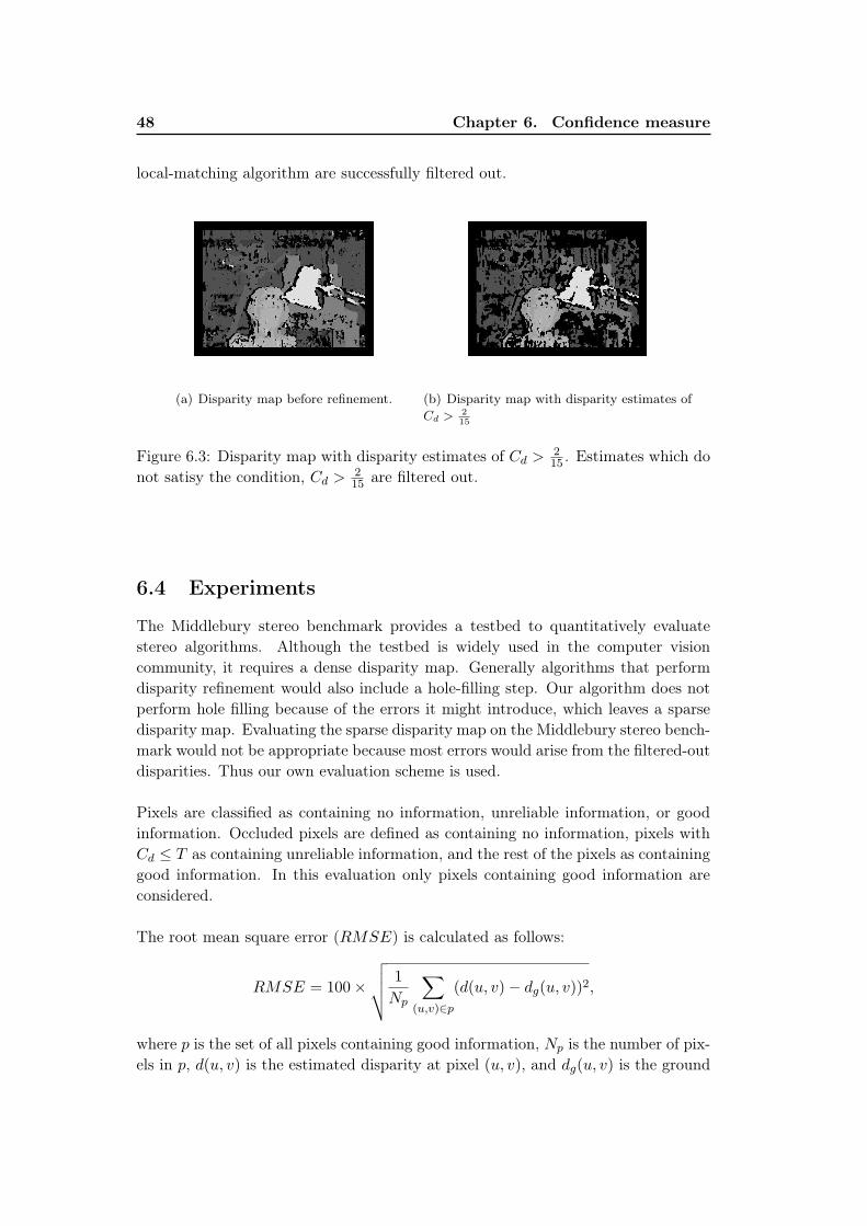
48 Chapter 6. Confidence measure
local-matching algorithm are successfully filtered out.
(a) Disparity map before refinement. (b) Disparity map with disparity estimates ofCd > 2
15
Figure 6.3: Disparity map with disparity estimates of Cd > 215 . Estimates which do
not satisy the condition, Cd > 215 are filtered out.
6.4 Experiments
The Middlebury stereo benchmark provides a testbed to quantitatively evaluatestereo algorithms. Although the testbed is widely used in the computer visioncommunity, it requires a dense disparity map. Generally algorithms that performdisparity refinement would also include a hole-filling step. Our algorithm does notperform hole filling because of the errors it might introduce, which leaves a sparsedisparity map. Evaluating the sparse disparity map on the Middlebury stereo bench-mark would not be appropriate because most errors would arise from the filtered-outdisparities. Thus our own evaluation scheme is used.
Pixels are classified as containing no information, unreliable information, or goodinformation. Occluded pixels are defined as containing no information, pixels withCd ≤ T as containing unreliable information, and the rest of the pixels as containinggood information. In this evaluation only pixels containing good information areconsidered.
The root mean square error (RMSE) is calculated as follows:
RMSE = 100×
√√√√ 1
Np
∑(u,v)∈p
(d(u, v)− dg(u, v))2,
where p is the set of all pixels containing good information, Np is the number of pix-els in p, d(u, v) is the estimated disparity at pixel (u, v), and dg(u, v) is the ground

6.4. Experiments 49
Table 6.1: RMSE with a chosen window size, number of disparities, and thresholdT = 0 for the Middlebury dataset.
Image pair Window size Number of disparities T RMSE
Tsukuba 5× 5 15 0 7.56Venus 5× 5 19 0 29.84Teddy 9× 9 59 0 37.43Cones 9× 9 59 0 30.13
Table 6.2: RMSE for a chosen window size, an empirically selected T value andthe percentage computational overhead for the Middlebury dataset.
Image pair Window size T RMSE Computational overhead (%)Tsukuba 5× 5 2
15 6.56 2.33Venus 5× 5 4
19 21.94 18.35Teddy 9× 9 2
59 32.79 19.23Cones 9× 9 6
59 23.38 17.60
truth disparity at pixel (u, v).
The Middlebury dataset is used for evaluation. The results for this dataset onthe different image pairs with T = 0 are shown in Table 6.1. This table shows theimage pair used from the Middlebury dataset in the first column. The second andthird columns show the window size and the disparity search range used. The lasttwo columns show the T values and the RMSE. Table 6.2 shows results where thevalue of T is empirically selected based on a value giving the lowest RMSE. Thetable also shows the percentage computational overhead. This is the extra percent-age of computational time required for a chosen value of T compared to a value ofT = 0.
In the experiments it is noted that the RMSE starts increasing after a certainvalue of T for a selected window size. This is due to the errors introduced by thewindow size. Local-matching stereo algorithms assume constant disparity through-out the aggregation window, so errors known as the "foreground fattening" effect[2] arise. Also, since the images have pixel resolution, a window size greater than apixel affects the resolution of the disparity estimates. Errors are introduced wherethe image details are smaller than the window size. Since the algorithm does notfilter out these errors, they are fixed with a changing value of T . The larger thevalue of T , the smaller the value of Np while the errors remain fixed. A plot showingthe relationship between T and Np with a 5× 5 window size for the Tsukuba imagepair is shown in Figure 6.4.

50 Chapter 6. Confidence measure
0 0.1 0.2 0.3 0.4 0.5 0.6 0.70
1
2
3
4
5
6
7x 10
4
Threshold, T
num
ber
of p
ixel
s
Figure 6.4: Number of pixels Np versus Threshold (T ) with a 5× 5 window size forthe Tsukuba image pair.
0 0.05 0.1 0.15 0.2 0.25 0.3 0.35 0.4 0.45 0.50
5
10
15
20
25
30
Threshold, T
RM
SE
1x1 window size3x3 window size5x5 window size7x7 window size9x9 window size
Figure 6.5: Threshold T versus RMSE for varying window sizes.
To show the effect of the window size on the evaluation, Figure 6.5 contains a plotof T versus RMSE for varying window sizes. Different window sizes tend to shiftthe curve up or down. As the window size increases, the curve shifts downwardsuntil a point where a larger window introduces more errors, causing the curve toshift upwards.
6.5 Confidence measure in temporal seeding
In Chapter 5 temporal seeding is applied on a stereo image sequence. The startupdisparities for temporal seeding are calculated using a full disparity search on theKLT features of the left image in the first stereo image frame. In this section, the

6.5. Confidence measure in temporal seeding 51
confidences of the detected features in the first stereo image frame are determined.The features are then selected according to their confidences and used as the startupfeatures. Temporal seeding is then applied and the results are evaluated as in Chap-ter 5.
The results of the experiments are shown below. Figure 6.6 shows the numberof features which satisfy a particular confidence. For the same reason as in Section5.7, the number of tracked features decreases as the number of frames progresses.Also, the number of startup features are high for low confidence values and low forhigh confidence values.
Figure 6.7 shows the RMSE for every frame when using startup disparities with aparticular confidence. The results show that the shapes of the Figures 6.7(a)-6.7(e)are similar meaning that the confidence measure is not removing enough erroneouspoints in temporal seeding. The peak error becomes higher as Cd increases. Thismight be caused by the fact that features with a higher Cd value are tracked forlonger in the image sequence. This means the error is propagated longer in thesequence leading to a higher peak error. Figure 6.7(e) appears to have more noisecompared to the other plots. This is due to the low number of features which havea confidence value of 1.

52 Chapter 6. Confidence measure
0 10 20 30 40 50 60 70 80 900
200
400
600
800
1000
1200
1400
1600
number of frames
num
ber
of fe
atur
es
(a) Number of features with Cd ≥ 020
detectedon the stereo image sequence
0 10 20 30 40 50 60 70 80 900
200
400
600
800
1000
1200
1400
1600
number of frames
num
ber
of fe
atur
es(b) Number of features with Cd ≥ 5
20detected
on the stereo image sequence
0 10 20 30 40 50 60 70 80 900
200
400
600
800
1000
1200
1400
1600
number of frames
num
ber
of fe
atur
es
(c) Number of features with Cd ≥ 1020
detectedon the stereo image sequence
0 10 20 30 40 50 60 70 80 900
200
400
600
800
1000
1200
1400
1600
number of frames
num
ber
of fe
atur
es
(d) Number of features with Cd ≥ 1520
detectedon the stereo image sequence
0 10 20 30 40 50 60 70 80 900
200
400
600
800
1000
1200
1400
1600
number of frames
num
ber
of fe
atur
es
(e) Number of features with Cd ≥ 2020
detectedon the stereo image sequence
Figure 6.6: Number of features detected on the stereo image sequence which have achosen confidence.

6.5. Confidence measure in temporal seeding 53
0 10 20 30 40 50 60 70 80 900
10
20
30
40
50
60
70
number of frames
RM
SE
(a) RMSE for features with Cd ≥ 020
for thestereo image sequence
0 10 20 30 40 50 60 70 80 900
10
20
30
40
50
60
70
number of frames
RM
SE
(b) RMSE for features with Cd ≥ 520
for thestereo image sequence
0 10 20 30 40 50 60 70 80 900
10
20
30
40
50
60
70
number of frames
RM
SE
(c) RMSE for features with Cd ≥ 1020
for thestereo image sequence
0 10 20 30 40 50 60 70 80 900
10
20
30
40
50
60
70
number of frames
RM
SE
(d) RMSE for features with Cd ≥ 1520
for thestereo image sequence
0 10 20 30 40 50 60 70 80 900
10
20
30
40
50
60
70
number of frames
RM
SE
(e) RMSE for features with Cd ≥ 2020
for thestereo image sequence
Figure 6.7: RMSE versus the number of frames for different confidence values.


Chapter 7
Conclusions
Section 7.1 summarizes the main topics and the results of this work. Section 7.2discusses possible future work.
7.1 Conclusions
There are two main objectives of this work. The first objective is to investigatetemporal seeding in stereo image sequences. This is discussed in Chapter 5. Thesecond objective is to develop a confidence measure for local-matching stereo algo-rithms discussed in Chapter 6.
The stereo vision problem is discussed sequentially. It is pointed out that the mainproblem with stereo vision is the stereo correspondence problem. Relevant literaturefor this problem is discussed and the solution chosen to be explored is the use oflocal-matching stereo algorithms. These algorithms have a uniform structure andare applicable in real-time systems. They can also be broken down into componentswhich allows us to highlight the different design considerations. The usefulness ofbreaking down the algorithm into its components is discussed in Chapter 4. In or-der to meet the objectives, a central part in the stereo correspondence formulationin local-matching algorithms namely the correlation curve was investigated. Theanalysis of this curve provided interesting and useful information.
7.1.1 Temporal seeding
Chapter 5 presents a way of reusing computed disparity estimates of KLT featuresin a stereo image sequence. The temporal seeding approach developed makes useof the correlation curves of tracked KLT features. Two experiments are conducted.Firsly, only two stereo image frames are used. The results for this experiment showthat temporal seeding produces the same error as the implemented stereo algorithmbut does improve the computational overhead by approximately 30%.
The second experiment is done on 87 frames of a stereo image sequence. Fea-tures are tracked throughout the sequence and features which cannot be trackedare replaced by new ones. The temporal seeding is evaluated and the results showthat the RMSE increases as the number of frames increase. This is caused by error

56 Chapter 7. Conclusions
propagation. This means that the quality of the initial disparity estimates has to behigh to avoid error propagation. The error propagation rate decreases as the numberof frames increase. A possible cause for this is the fact that features which cannotbe tracked are replaced with new features. The computational time of the temporalseeding algorithm is approximately 20% faster than Birchfield and Tomasi’s stereoalgorithm.
7.1.2 Confidence measure
Chapter 6 presents a confidence measure to detect textureless regions for local-matching algorithms. The confidence measure is formulated by analysing a propertyof the correlation curve called the basin of convergence. The effectiveness of thisapproach is demonstrated by implementing a local-matching algorithm and filteringout unreliable depth estimates. The quantitative evaluation demonstrated that theconfidence measure decreases the disparity estimate errors at a small computationalcost.
Further experiments involve using the confidence measure in temporal seeding. Thedetected KLT features are selected based on their confidence. These features arethen used as start-up features for temporal seeding. The results show that the con-fidence measure does not succeed in removing features which produce high errors.
7.2 Future work
The main problem with temporal seeding is error propagation. This can be overcomeby performing the temporal seeding process for a certain number of frames then us-ing the stereo algorithm to determine new start-up disparities. Also, the temporalseeding approach is done on KLT features which means that a sparse disparity mapis obtained. Ultimately, it would be very useful to have a denser disparity map.Instead of using the confidence measure on KLT features, one might consider usingit as a feature detector. This would provide denser results for temporal seeding.
The temporal seeding approach developed is for local-matching stereo algorithms.Developing a temporal seeding approach for slower algorithms such as graph cutswill aid in decreasing the computational time in the hope of making the algorithmrun in real-time.
Since the temporal seeding approach is used in a sparse context, it may be use-ful in applications such as motion estimation. Exploring such an application mightresult in a faster algorithm.

Bibliography
[1] D. Scharstein and R. Szeliski, “Middlebury stereo vision page,” August 2009,vision.middlebury.edu/stereo/. vii, 2, 21, 45
[2] D. Scharstein, R. Szeliski, and R. Zabih, “A taxonomy and evaluation of densetwo-frame stereo correspondence algorithms,” in Proceedings of the IEEE Work-shop on Stereo and Multi-Baseline Vision. Washington, DC, USA: IEEE Com-puter Society, 2001, p. 131. 1, 3, 6, 7, 21, 29, 49
[3] M. Z. Brown, D. Burschka, and G. D. Hager, “Advances in computationalstereo,” IEEE Transactions on Pattern Analysis and Machine Intelligence,vol. 25, pp. 993–1008, August 2003. 1
[4] L. Linhui, Z. Mingheng, G. Lie, and Z. Yibing, “Stereo vision based obstacleavoidance path-planning for cross-country intelligent vehicle,” in Proceedings ofthe 6th international conference on Fuzzy systems and knowledge discovery, ser.FSKD’09. Piscataway, NJ, USA: IEEE Press, 2009, pp. 463–467. 1
[5] T. Lemaire, C. Berger, I.-K. Jung, and S. Lacroix, “Vision-based slam: Stereoand monocular approaches,” International Journal on Computer Vision, vol. 74,pp. 343–364, September 2007. 1
[6] M. Kanbara, H. Fujii, H. Takemura, and N. Yokoya, “A stereo vision-basedaugmented reality system with an inertial sensor,” International Symposium onAugmented Reality, vol. 0, p. 97, 2000. 1
[7] V. I. Pavlovic, R. Sharma, and T. S. Huang, “Visual interpretation of handgestures for human-computer interaction: A review,” IEEE Transactions onPattern Analysis and Machine Intelligence, vol. 19, pp. 677–695, July 1997. 2
[8] L. Stefano, “A fast area-based stereo matching algorithm,” Image and VisionComputing, vol. 22, no. 12, pp. 983–1005, 2004. 3, 25
[9] L. Di Stefano, M. Marchionni, and S. Mattoccia, “A pc-based real-time stereovision system,” International Journal on Machine Graphics and Vision, vol. 13,pp. 197–220, January 2004. 3, 25
[10] F. Tombari, S. Mattoccia, and L. Di Stefano, “Segmentation-based adaptivesupport for accurate stereo correspondence,” in Proceedings of the 2nd PacificRim conference on Advances in image and video technology, ser. PSIVT’07.Berlin, Heidelberg: Springer-Verlag, 2007, pp. 427–438. 4, 23, 31
[11] R. Yang, M. Pollefeys, and S. Li, “Improved real-time stereo on commoditygraphics hardware,” in Proceedings of the 2004 Conference on Computer Visionand Pattern Recognition Workshop, vol. 3. Washington, DC, USA: IEEEComputer Society, 2004, pp. 36–. 4

58 Bibliography
[12] J. Woodfill and B. Von Herzen, “Real-time stereo vision on the parts reconfig-urable computer,” in Proceedings of the 5th IEEE Symposium on FPGA-BasedCustom Computing Machines. Washington, DC, USA: IEEE Computer Soci-ety, 1997, pp. 201–. 4
[13] Y. Boykov, O. Veksler, and R. Zabih, “Fast approximate energy minimizationvia graph cuts,” IEEE Transactions Pattern Analysis and Machine Intelligence,vol. 23, pp. 1222–1239, November 2001. 4
[14] S. Roy and I. J. Cox, “A maximum-flow formulation of the n-camera stereocorrespondence problem,” in Proceedings of the Sixth International Conferenceon Computer Vision, ser. ICCV ’98. Washington, DC, USA: IEEE ComputerSociety, 1998, pp. 492–. 4
[15] V. Kolmogorov and R. Zabih, “Computing visual correspondence with occlu-sions using graph cuts,” IEEE International Conference on Computer Vision,vol. 2, p. 508, 2001. 4
[16] O. Veksler, “Efficient graph-based energy minimization methods in computervision,” Ph.D. dissertation, Ithaca, NY, USA, 1999, aAI9939932. 4
[17] R. B. Potts, “Some Generalized Order-Disorder Transformation,” in Transfor-mations, Proceedings of the Cambridge Philosophical Society, vol. 48, 1952, pp.106–109. 4
[18] A. F. Bobick and S. S. Intille, “Large occlusion stereo,” International Journalof Computer Vision, vol. 33, pp. 181–200, September 1999. 5
[19] I. J. Cox, S. L. Hingorani, S. B. Rao, and B. M. Maggs, “A maximum likelihoodstereo algorithm,” Computer Vision and Image Understanding, vol. 63, pp. 542–567, May 1996. 5
[20] D. Geiger, B. Ladendorf, and A. Yuille, “Occlusions and binocular stereo,”International Journal of Computer Vision, vol. 14, pp. 211–226, April 1995. 5
[21] A. L.Yuille and T. Poggio, “A generalized ordering constraint for stereo corre-spondence,” MIT, A.I.Memo 777, 1984, aI Lab. 7, 27
[22] Z.-F. Wang and Z.-G. Zheng, “A region based stereo matching algorithm usingcooperative optimization,” IEEE Computer Society Conference on ComputerVision and Pattern Recognition, vol. 0, pp. 1–8, 2008. 7, 21
[23] A. Klaus, M. Sormann, and K. Karner, “Segment-based stereo matching usingbelief propagation and a self-adapting dissimilarity measure,” in Proceedings ofthe 18th International Conference on Pattern Recognition, ser. ICPR ’06, vol. 3.Washington, DC, USA: IEEE Computer Society, 2006, pp. 15–18. 7, 21

Bibliography 59
[24] H. Hirschmuller, P. R. Innocent, and J. Garibaldi, “Real-time correlation-basedstereo vision with reduced border errors,” International Journal of ComputerVision, vol. 47, pp. 229–246, April 2002. 8
[25] T. Kanade and M. Okutomi, “A stereo matching algorithm with an adaptivewindow: Theory and experiment.” IEEE Transactions on Pattern Analysis andMachine Intelligence. 8, 29
[26] J. C. Kim, K. M. Lee, B. T. Choi, and S. U. Lee, “A dense stereo matchingusing two-pass dynamic programming with generalized ground control points,”in Proceedings of the 2005 IEEE Computer Society Conference on ComputerVision and Pattern Recognition, ser. CVPR ’05, vol. 2. Washington, DC,USA: IEEE Computer Society, 2005, pp. 1075–1082. 8
[27] F. Tombari, S. Mattoccia, L. di Stefano, and E. Addimanda, “Near real-timestereo based on effective cost aggregation,” in International Conference on Pat-tern Recognition, 2008, pp. 1–4. 10, 24
[28] P. Anandan, “Computing dense displacement fields with confidence measuresin scenes containing occlusion,” Image Understanding Workshop, vol. 84, pp.236–246, 1984. 10, 45
[29] ——, “A computational framework and an algorithm for the measurement ofvisual,” Amherst, MA, USA, Tech. Rep., 1987. 10, 45
[30] R. I. Hartley and A. Zisserman, Multiple View Geometry in Computer Vision,2nd ed. Cambridge University Press, ISBN: 0521540518, 2004. 12, 16
[31] Z. Zhang, “A flexible new technique for camera calibration,” IEEE Transac-tions on Pattern Analysis and Machine Intelligence, vol. 22, pp. 1330–1334,November 2000. 13
[32] D. G. R. Bradski and A. Kaehler, Learning opencv, 1st ed. O’Reilly Media,Inc., 2008. 13
[33] J. Y. Bouguet, “Camera Calibration Toolbox for Matlab,” 2008. [Online].Available: http://www.vision.caltech.edu/bouguetj/calib_doc/. 13, 14, 17
[34] C. Harris and M. Stephens, “A combined corner and edge detector,” in Proceed-ings of the 4th Alvey Vision Conference, 1988, pp. 147–151. 13
[35] D. Comaniciu and P. Meer, “Mean shift: A robust approach toward featurespace analysis,” IEEE Transactions on Pattern Analysis and Machine Intelli-gence, vol. 24, pp. 603–619, May 2002. 21
[36] Q. Yang, L. Wang, R. Yang, H. Stewénius, and D. Nistér, “Stereo matchingwith color-weighted correlation, hierarchical belief propagation, and occlusionhandling,” IEEE Transactions of Pattern Analysis and Machine Intelligence,vol. 31, pp. 492–504, March 2009. 21, 22

60 Bibliography
[37] G. Egnal and R. P. Wildes, “Detecting binocular half-occlusions: Empiricalcomparisons of five approaches,” IEEE Transactions on Pattern Analysis andMachine Intelligence, vol. 24, no. 8, pp. 1127–1133, 2002. 21, 30, 45
[38] K. Konolige, “Small vision systems: hardware and implementation,” in EighthInternational Symposium on Robotics Research, 1997, p. 111–116. 21, 30, 45
[39] L. Xu and J. Jia, “Stereo matching: An outlier confidence approach,” in Euro-pean Conference on Computer Vision. Springer, 2008, pp. 775–787. 22
[40] Y. Taguchi, B. Wilburn, and C. L. Zitnick, “Stereo reconstruction with mixedpixels using adaptive over-segmentation,” IEEE Computer Society Conferenceon Computer Vision and Pattern Recognition, pp. 1–8, 2008. 22
[41] J. Sun, Y. Li, S. B. Kang, and H.-Y. Shum, “Symmetric stereo matching forocclusion handling,” in Proceedings of the 2005 IEEE Computer Society Con-ference on Computer Vision and Pattern Recognition, ser. CVPR ’05. Wash-ington, DC, USA: IEEE Computer Society, 2005, pp. 399–406. 22
[42] Q. Yang, C. Engels, and A. Akbarzadeh, “Near real-time stereo for weakly-textured scenes,” in Proceedings of the British Machine Vision Conference,2008, pp. 80–87. 22
[43] Z. Gu, X. Su, Y. Liu, and Q. Zhang, “Local stereo matching with adaptivesupport-weight, rank transform and disparity calibration,” Pattern RecognitionLetters, vol. 29, pp. 1230–1235, July 2008. 22
[44] H. Hirschmuller, “Stereo vision in structured environments by consistent semi-global matching,” IEEE Computer Society Conference on Computer Vision andPattern Recognition, vol. 2, pp. 2386–2393, 2006. 23
[45] S. Mattoccia, F. Tombari, and L. Di Stefano, “Stereo vision enabling preciseborder localization within a scanline optimization framework,” in Proceedingsof the 8th Asian conference on Computer vision, ser. ACCV’07, vol. 2. Berlin,Heidelberg: Springer-Verlag, 2007, pp. 517–527. 23
[46] K.-J. Yoon and I. S. Kweon, “Stereo matching with the distinctive similaritymeasure,” IEEE International Conference on Computer Vision, pp. 1–7, 2007.23
[47] C. Lei, J. Selzer, and Y.-H. Yang, “Region-tree based stereo using dynamicprogramming optimization,” in Proceedings of the 2006 IEEE Computer SocietyConference on Computer Vision and Pattern Recognition, ser. CVPR ’06, vol. 2.Washington, DC, USA: IEEE Computer Society, 2006, pp. 2378–2385. 23
[48] K.-J. Yoon and I. S. Kweon, “Adaptive support-weight approach for correspon-dence search,” IEEE Transactions on Pattern Analysis and Machine Intelli-gence, vol. 28, pp. 650–, April 2006. 23

Bibliography 61
[49] A. Bhusnurmath and C. J. Taylor, “Solving stereo matching problems usinginterior point methods,” in Fourth International Symposium on 3D Data Pro-cessing, Visualization and Transmission, O. S. Stefan Gumhold, Jana Kosecka,Ed., June 2008, pp. 321–329. 23
[50] S. K. Gehrig and U. Franke, “Improving stereo sub-pixel accuracy for long rangestereo,” IEEE International Conference on Computer Vision, pp. 1–7, 2007. 23
[51] H. Hirschmuller, “Accurate and efficient stereo processing by semi-global match-ing and mutual information,” IEEE Computer Society Conference on ComputerVision and Pattern Recognition, vol. 2, pp. 807–814, 2005. 24
[52] Q. Yang, L. Wang, R. Yang, S. Wang, M. Liao, and D. Nistér, “Real-timeglobal stereo matching using hierarchical belief propagation,” in Proccedings ofthe British Machine Vision Conference. British Machine Vision Association,2006, pp. 989–998. 24
[53] T. Liu, P. Zhang, and L. Luo, “Dense stereo correspondence with contrast con-text histogram, segmentation-based two-pass aggregation and occlusion han-dling,” in Proceedings of the 3rd Pacific Rim Symposium on Advances in Imageand Video Technology, ser. PSIVT ’09. Berlin, Heidelberg: Springer-Verlag,2008, pp. 449–461. 24
[54] J. Lu, G. Lafruit, and F. Catthoor, “Anisotropic local high-confidence voting foraccurate stereo correspondence.” in Image Processing: Algorithms and Systems,2008, p. 1. 24
[55] P. Mordohai and G. Medioni, “Stereo using monocular cues within the ten-sor voting framework,” IEEE Transactions on Pattern Analysis and MachineIntelligence, vol. 28, pp. 968–982, June 2006. 24
[56] L. Wang, M. Liao, M. Gong, R. Yang, and D. Nister, “High-quality real-timestereo using adaptive cost aggregation and dynamic programming,” in Pro-ceedings of the Third International Symposium on 3D Data Processing, Visu-alization, and Transmission, ser. 3DPVT ’06. Washington, DC, USA: IEEEComputer Society, 2006, pp. 798–805. 24
[57] O. Veksler, “Stereo correspondence by dynamic programming on a tree,” in Pro-ceedings of the 2005 IEEE Computer Society Conference on Computer Visionand Pattern Recognition, ser. CVPR ’05, vol. 2. Washington, DC, USA: IEEEComputer Society, 2005, pp. 384–390. 24
[58] S. Birchfield and C. Tomasi, “A pixel dissimilarity measure that is insensitiveto image sampling,” IEEE Transactions on Pattern Analysis and Machine In-telligence, vol. 20, no. 4, pp. 401–406, 1998. 26, 36

62 Bibliography
[59] H. Hirschmuller and D. Scharstein, “Evaluation of stereo matching costs onimages with radiometric differences,” IEEE Transactions on Pattern Analysisand Machine Intelligence, vol. 31, no. 9, pp. 1582–1599, 2009. 26
[60] L. Wang, M. Gong, M. Gong, and R. Yang, “How far can we go with localoptimization in real-time stereo matching,” in Proceedings of the Third Inter-national Symposium on 3D Data Processing, Visualization, and Transmission.Washington, DC, USA: IEEE Computer Society, 2006, pp. 129–136. 28
[61] J. J. Little and W. E. Gillett, “Direct evidence for occlusion in stereo andmotion,” in Proceedings of the First European Conference on Computer Vision.London, UK: Springer-Verlag, 1990, pp. 336–340. 30, 45
[62] A. Luo and H. Burkhardt, “An intensity-based cooperative bidirectional stereomatching with simultaneous detection of discontinuities and occlusions,” Inter-national Journal of Computer Vision, vol. 15, no. 3, pp. 171–188, 1995. 30,45
[63] Q. Yang, R. Yang, J. Davis, and D. Nister, “Spatial-depth super resolution forrange images,” IEEE Conference on Computer Vision and Pattern Recognition,pp. 1–8, 2007. 30
[64] S. W. Zucker and R. A. Hummel, “Toward a Low-level Description of Dot Clus-ters: Labeling Edge, Interior, and Noise Points,” Computer Vision, Graphics,and Image Processing, vol. 9, no. 3, pp. 213–233, March 1979. 31
[65] N. Ahuja and M. Tuceryan, “Extraction of early perceptual structure in dotpatterns: integrating region, boundary, and component gestalt,” Computer Vi-sion, Graphics, and Image Processing, vol. 48, pp. 304–356, December 1989.31
[66] N. Thacker and P. Courtney, “Statistical analysis of a stereo matching algo-rithm,” in Proceedings of the British Machine Vision Conference, 1992, pp.316–326. 33
[67] L. Matthies and M. Okutomi, “Bootstrap algorithms for dynamic stereo vision,”in Proceedings of the 6th Multidimensional Signal Processing Workshop, 1989,p. 12. 34
[68] A. Dalmia and M. Trivedi, “High speed extraction of 3d structure of selectablequality using a translating camera,” Computer Vision and Image Understand-ing, vol. 64, no. 1, pp. 97–110, 1996. 34
[69] S. T. G. Xu and M. Asada, “A motion stereo method based on coarse to finecontrol strategy,” IEEE Transactions on Pattern Analysis and Machine Intel-ligence, vol. 9, no. 2, pp. 332–336, 1987. 34

Bibliography 63
[70] B. C. L. Zhang and S. Seitz, “Spacetime stereo: Shape recovery for dynamicscenes,” in Proceedings of IEEE Computer Society Conference on ComputerVision and Pattern Recognition, 2003, pp. 367–374. 34
[71] R. R. S. R. J. Davis, D. Nehab, “Spacetime stereo : A unifying framework fordepth from triangulation,” IEEE Transaction On Pattern Analysis and MachineIntelligence, vol. 27, no. 2, 2005. 34
[72] N. T. S. Crossley and N. Seed, “Benchmarking of bootstrap temporal stereousing statistical and physical scene modelling,” in Proceedings of the BritishMachine Vision Conference, 1998, pp. 346–355. 34
[73] N. T. S. Crossley, A.J. Lacey and N. Seed, “Robust stereo via temporal con-sistency,” in Proceedings of the British Machine Vision Conference, 1997, pp.659–668. 34
[74] D. B. L. Kanade and T. Kanade, “An iterative image registration technique withan application to stereo vision,” in International Joint Conference on ArtificialIntelligence, 1981, pp. 674–679. 35
[75] C. Tomasi and T. Kanade, “Detection and tracking of point features,” Tech.Rep., 1991. 36
[76] J. Shi and C. Tomasi, “Good features to track,” in IEEE Conference on Com-puter Vision and Pattern Recognition, 1994, pp. 593–600. 36
[77] “Microsoft i2i dataset,” http://research.microsoft.com/en-us/projects/i2i.41
[78] R. Trapp, S. Drüe, and G. Hartmann, “Stereo matching with implicit detectionof occlusions,” in Proceedings of the 5th European Conference on ComputerVision, vol. 2. London, UK: Springer-Verlag, 1998, pp. 17–33. 45
[79] M. J. Hannah, “Computer matching of areas in stereo images.” Ph.D. disserta-tion, Stanford, CA, USA, 1974. 45
[80] D. Smitley and R. Bajcsy, “Stereo processing of aerial, urban images,” Interna-tional Conference on Pattern Recognition, vol. 84, pp. 433–435, 1984. 45
[81] J. J. Little and W. E. Gillett, “Direct evidence for occlusion in stereo andmotion,” in Proceedings of the First European Conference on Computer Vision.London, UK: Springer-Verlag, 1990, pp. 336–340. 45
[82] D. Scharstein, “View synthesis using stereo vision,” Ph.D. dissertation, Ithaca,NY, USA, 1997. 45
[83] Y. G. Leclerc, “Constructing Simple Stable Descriptions for Image Partition-ing,” International Journal of Computer Vision, vol. 3, no. 1, pp. 73–102, 1989.46

64 Bibliography
[84] D. Samaras, D. Metaxas, P. Ascalfua, and Y. G. Leclerc, “Variable albedo sur-face reconstruction from stereo and shape from shading,” in IEEE Conferenceon Computer Vision and Pattern Recognition, 2000, pp. 480–487. 46
[85] R. Gherardi, “Confidence-based cost modulation for stereo matching,” in Inter-national Conference on Pattern Recognition, 2008, pp. 1–4. 46