An Investigation into Flow Properties of Self‐Healing Agents 

in Damaged Zones of Cementitious Materials 

 

 

A thesis submitted for the Degree of Master of Philosophy 

 

 

by 

Andrea Hoffman B.Eng. (Hons) 

 

 

 

School of Engineering 

 

 

 

May 2012 

i

Acknowledgements 

 

 

The support that has been given to me from my family throughout the whole of 

this MPhil has been incredible, so therefore I would like to dedicate this thesis to 

them. 

 

Dr.  Diane  Gardner,  my  supervisor  for  this  research  project  has  assisted  me 

through learning and she has taught me a lot and not just in the studies looked at 

in this thesis.    I feel that  I have made such a  large progression  in my education 

and  skills  from  this  MPhil  and  would  like  to  thank  her  for  this  as  she  has 

encouraged and guide me every step of the way.  Thank you. 

 

I would also like to thank my personal tutor, lecturer and other supervisor, Dr. A. 

D. Jefferson.  Throughout my time at university he has provided me with the best 

guidance any supervisor or  tutor ever could and without his help and  support, 

this would not have been possible.  Thank you. 

 

The technician staff; Carl, Iain, Harry, Des, Brian and Len have been amazing and I 

have enjoyed every minute down  in the  laboratory with them.   They have been 

so amazing and helpful and  I cannot  thank  them enough.    I had  the best  time 

down  in  the  labs with Carl and  Iain and  they have made  this an unforgettable 

experience.  I would also  like to thank Len,  for putting up with me when  I used 

the scales from his lab without asking and not returning them and also Harry for 

all of his hard work and expertise down in the lab helping me with experimental 

difficulties. 

 

Lastly, I would like to thank everyone in office W1.32, Iulia, Ben, Simon D, Simon 

C, Adrianna and Rob; you guys have been amazing and are  friends  I will never 

forget.  

 

 

ii

  DECLARATION  This work has not previously been accepted in substance for any degree and is not concurrently submitted in candidature for any degree.  Signed ………………………………………………………            Date ……18/05/2012   STATEMENT 1  This  thesis  is being  submitted  in partial  fulfillment of  the  requirements  for  the degree of MPhil  Signed ………………………………………………………            Date ……18/05/2012   STATEMENT 2  This  thesis  is  the  result  of  my  own  independent  work/investigation,  except where otherwise stated. Other sources are acknowledged by explicit references.    Signed ………………………………………………………            Date ……18/05/2012   STATEMENT 3  I hereby give consent for my thesis, if accepted, to be available for photocopying and for inter‐library loan, and for the title and summary to be made available to outside organisations.  Signed ………………………………………………………            Date ……18/05/2012  

 

 

 

 

 

iii

Summary 

 

 

 

This thesis is concerned with the experimental and numerical study of capillarity 

in cementitious materials.  Capillarity is a phenomenon that has been researched 

by  many;  however,  literature  shows  few  studies  completed  on  capillarity  in 

cementitious  materials,  in  particular  discrete  cracks.    This  thesis  presents 

experimental and numerical data to further those areas in research that rely on 

capillary flow mechanisms, such as the deterioration process in concrete and the 

flow of healing agents in self‐healing cementitious materials. 

   

Experimental  simulations  of  capillary  flow  through  five  different  crack 

configurations  in  cementitious  materials  have  been  studied.    Alongside  the 

experimental  work  capillary  flow  theory  has  been  used  to  validate  the 

experimental  results with  the use of numerical  formulae.   This  thesis presents 

details of the Lucas‐Washburn equation traditionally used in capillarity and glue 

flow  theory  in chapter 5 and  the experimental results alongside  the  theory are 

used to assess the performance of the numerical models. 

 

Some of the conclusions that have been made are listed below however, a more 

in depth view is shown in chapter 4: 

• results  looking  at  the effect of  crack  configuration  show  that  the  crack 

path does not have a large effect on capillarity; 

• specimen age of mortar was another area that was looked at and results 

and readings do show that the rate of rise is affected by age; 

• the  difference  between  the  healing  agents  used  in  experiments  does 

show that viscosity does play a large part in rate of capillarity and 

• specimen saturation, one of the parameters also touched on in this thesis 

does show that the more saturated the specimen, the higher the flow of 

the healing agent. 

 

iv

Conclusions are made and are presented  in chapter 6 based on  the analysis of 

the  experimental  results  and  the  validation  of  the  numerical  solution.  

Comparisons between the experimental work and numerical solution show that 

the numerical  solution  for various crack configurations  is  reliable  to determine 

the glue flow theory for healing agents. 

 

 

 

 

 

 

 

 

 

 

 

 

 

 

 

 

 

 

 

 

 

v

Contents 

 

 

  Page 

Number 

Acknowledgements  i 

Declaration  ii 

Summary  iii 

Contents  v 

List of tables    ix 

List of figures    x 

Main notation    xv 

 

Chapter 1 

 

 

1.1 Introduction  1 

1.2 Aims of work  3 

1.3 Layout of the Thesis 

 

3 

Chapter 2 

 

 

2.1 Introduction to State of the Art Review  5 

2.2 Causes of concrete decay 30 years ago  6 

2.3 Carbonation of concrete   7 

2.4 Permeability of concrete  9 

2.5 Corrosion of concrete  12 

2.6 Chloride attack  14 

2.7 Capillarity  16 

   2.7.1 Introduction to capillary action  16 

   2.7.2 Surface tension, cohesion and adhesion  16 

   2.7.3 Sorptivity  17 

vi

 

   2.7.4 Equation of capillarity 

Page no. 

20 

   2.7.5 Capillary flow and contact angles  24 

   2.7.6 Capillarity and cementitious materials  27 

   2.7.7 Kinetics of capillary absorption  28 

2.8 Self healing cementitious materials  30 

   2.8.1 Definitions  30 

   2.8.2 Autogenic healing studies  31 

   2.8.3 Autonomic healing studies 

2.9 Final literature summary 

 

33 

35 

Chapter 3 

 

 

3.1 Introduction  36 

3.2 Materials  37 

3.3 Specimen manufacture  38 

   3.3.1 Specimen numbers and form  38 

3.4 Casting  39 

   3.4.1 Mix procedure  39 

   3.4.2 Specimen curing  39 

3.5 Crack configurations and apertures  41 

   3.5.1. Planar and tapered cracks  41 

   3.5.2 Tortuous crack investigation  42 

   3.5.3 Natural crack configuration  43 

3.6 Flow agents  44 

   3.6.1 Water and Cyanoacrylate  44 

   3.6.2 Xanthan gum  45 

3.7 Experimental details  45 

   3.7.1 Data capturing technique  45 

   3.7.2 Lighting  46 

   3.7.3 Experimental arrangement  47 

   3.7.4 Data Processing  49 

vii

Chapter 4 

 

Page no. 

4.1 Introduction  50 

4.2 Effect of crack configuration  57 

4.3 Effect of flow agent  66 

4.4 Effect of specimen age  78 

4.5 Effect of specimen saturation results and discussions  

4.6 Main concluding results 

   4.6.1 Equivalent planar crack for natural cracks 

   4.6.2 Effectiveness of cyanoacrylate flow and potential to heal 

4.7 Summary of conclusions 

 

85 

86 

86 

88 

88 

 

Chapter 5 

 

 

5.1 Basic capillary flow equations   90 

5.2 Analysis of the Lucas‐Washburn equation  91 

5.3 Numerical solution  92 

   5.3.1 Time stepping algorithm  94 

5.4 Planar and Tapered capillary fluid flow  95 

   5.4.1 Numerical solution of flow equation for planar and tapered   

fluid flow 

95 

5.5 Validation of the numerical model  96 

5.6 Validation of experimental results with theory  98 

    5.6.1 Planar fluid flow  98 

    5.6.2 Tapered fluid flow  103 

5.7 Conclusions 

 

Chapter 6 

 

105 

6.1 Introduction  106 

6.2 Conclusions  106 

   6.2.1 Capillary flow experimentation and conclusions  107 

viii

 

   6.2.2 Effect of crack configuration 

Page  no. 

   107 

   6.2.3 Effect of flow agent  108 

   6.2.4 Effect of specimen age  109 

   6.2.5 Effect of specimen saturation  109 

6.3 Numerical models and validity of results  109 

6.4 Recommendations for further work  110 

References  112 

Appendix A   

Appendix B   

Appendix C   

Appendix D   

 

 

 

 

 

 

 

 

 

 

 

 

 

 

 

 

ix

List of tables  

 

 

 

Chapter 3 

 

Page 

number 

Table 1:   Calculation of sand grading for dry sieving. 37

Table 2:   Specimen numbers and form. 38

Table 3:   Physical  properties  of  flow  agents  used  in  the 

experimental work 

44

Table 4:   Quantities of fluid used in each experiment. 49

     

Chapter 4   

   

Table 5:   Changes in weight of 28 day planar water experiments.  53

Table 6:  Calculation  of  crack  apertures  used  in  experimental 

work. 

58

Table 7:  Comparing  crack  apertures  for  mature  natural  crack 

aperture experiments. 

63

Table 8:  Comparison of cyanoacrylate theoretical rise height with   

experimental rise height. 

72

Table 9:  Crack aperture calculation. 88

 

Chapter 5 

 

 

Table 10:  Calculation of viscosity 102

   

   

   

   

x

List of figures 

 

 

 

Chapter 2  Page 

number 

Figure 1:  Process of carbonation through cementitious materials – 

based on literature from Bernard (2004). 

7

Figure 2:  Flow of water through porous media Song et al. (2007)  10

Figure 3:  Crack positions generated for experimental work Granju 

et al. (2005) 

13

Figure 4:  a) cohesion forces are less than adhesion & b) adhesion    

forces are greater than cohesion 

17

Figure 5:  Capillary flow adapted from Liou et. Al. 2009 21

Figure 6:  Adapted from Funada and Joseph (2002), instability of 

viscous flow in a capillary. 

22

Figure 7:  Fluid on solid planar surface. 25

Figure 8:  Image of experimental set up to determine contact angle 

of liquid‐solid interface 

26

Figure 9   Autonomic healing concept for cyanoacrylate adapted 

from Joseph et al. (2010) 

35

   

Chapter 3   

Figure 10:  A  Schematic  representation of  a) planar  and b)  tapered 

crack configuration. 

41

Figure 11:  Tapered  crack  of  a)  3  nodes  and  b)  5  nodes  achieved 

using folded steel plates. 

42

Figure 12:  Manufacture  of  naturally  cracked  specimens  a)  Three 

point bend  test arrangement b) Extraction of  specimens 

from cracked zone of prism 

43

Figure 13:  Image of natural  crack experimental arrangement under 

UV lighting 

47

Figure 14:   Experimental arrangement 48

xi

Chapter 4  Page 

number 

Figure 15:  Capillary  rise  front  for  old  planar  water  with  a  crack 

aperture of 0.502 mm a) 16mm at 0s b) 19mm at 0.036s 

c) 21mm at 0.072s d) 24mm at 0.160s e) 30mm at 0.716s 

f) 33.8mm at 5.600s 

51

Figure 16:  35 day planar water experimental results 51

Figure 17:  Measured  Crack  apertures  for  a  crack  aperture  of  a) 

0.094mm and b) 0.110mm. 

52

Figure 18:  Difference  in  maximum  rise  heights  and  changes  in 

weight  of  old  planar  water  0.261mm  aperture  over  a 

period of 3 seconds showing fluid absorption into cement 

matrix. 

54

Figure 19:  Comparison of planar crack aperture with final rise 

heights for 35 day old specimens 

55

Figure 20:  Gradient of the initial rise height over a period of 1 

second for 35 day old planar specimens. 

56

Figure 21:  35 day tapered water experimental graphs and results  57

Figure 22:  Effect of crack configuration, 35 day tortuous 3 nodes 

water and 35 day tortuous 5 nodes water 

59

Figure 23:  Comparison of tortuous crack aperture with final rise 

heights for 35 day old specimens 

60

Figure 24:  Gradient of the initial rise response over a period of 1 

second for 35 day old tortuous 3 and 5 node specimens 

with water. 

61

Figure 25:  35 day natural water experimental graph and results  62

Figure 26:  Crack apertures of (a) 0.170mm and (b) 0.261mm for 

tortuous experiments of 2 and 5 nodes 

64

Figure 27:  Old planar water, old  tapered water, old  tortuous water 

and  old  natural  water  experimental  results  from  0‐8 

seconds for a crack aperture of 0.344mm 

65

Figure 28:  Old planar water, old  tapered water, old  tortuous water 

and  old  natural  water  experimental  results  from  0‐8 

seconds for a crack aperture of 0.502mm 

65

   

xii

  Page 

Number

Figure 29:  Old planar water, old  tapered water, old  tortuous water 

and  old  natural  water  experimental  results  from  0‐8 

seconds for a crack aperture of 0.714mm 

66

Figure 30:   35 day mature planar water and old planar cyanoacrylate 

experimental results 

67

Figure 31:  Comparison of 35 day cyanoacrylate planar experimental 

final rise height data over a range of crack apertures with 

theoretical data 

68

Figure 32:  Gradient of the initial rise response over a period of 1 

second for 35 day old planar specimens using 

cyanoacrylate. 

69

Figure 33:  Comparison  of  35  day  cyanoacrylate  tortuous 

experimental  final  rise height data over a  range of crack 

apertures with theoretical data 

70

Figure 34:  Gradient  of  the  initial  rise  response  over  a  period  of  1 

second for 35 day old tortuous specimens. 

71

Figure 35:  35  day  mature  specimens  tapered  water  and  35  day 

mature  specimens  tapered  cyanoacrylate  experimental 

results 

72

Figure 36:  Effect of flow agent: 35 day mature tortuous 3 nodes 

water and 35 day mature tortuous 3 nodes cyanoacrylate 

74

Figure 37:  Absorption into specimens in experiments 74

Figure 38:  Effect of flow agent: old tortuous 5 nodes water and old 

tortuous  5  nodes  cyanoacrylate  experimental  graphical 

results 

75

Figure 39:  Effect of flow agent: Old planar xanthan gum, old planar 

water and old planar cyanoacrylate 

76

Figure 40:  Graph of capillary rise rates  for xanthan gum, water and 

cyanoacrylate 

77

Figure 41:  Effect of age, old planar water and young planar water 

graphical results 

78

   

   

xiii

Page 

number 

Figure 42:  Comparison  of  planar  crack  aperture  with  final  rise 

heights for 7 and 35 day old specimens using water 

79

Figure 43:  Gradient  of  the  initial  rise  response  over  a  period  of  1 

second  for  7  and  35  day  old  planar  specimens  using 

water. 

80

Figure 44:  Effect of age: old tapered water and young tapered water  81

Figure 45:  Effect of age: Old planar cyanoacrylate and young planar 

cyanoacrylate 

82

Figure 46:  Comparison  of  planar  crack  aperture  with  final  rise 

heights  for  7  and  35  day  old  specimens  using 

cyanoacrylate   

83

Figure 47:  Gradient  of  the  initial  rise  response  over  a  period  of  1 

second  for  7  and  35  day  old  planar  specimens  using 

cyanoacrylate. 

83

Figure 48:  Effect  of  Age:  Old  tapered  cyanoacrylate  and  young 

tapered cyanoacrylate 

84

Figure 49:  Effect of specimen saturation old planar water saturated 

and unsaturated 

85

Figure 50:  Comparison of natural cracks for planar cracks 86

Figure 51:  Graph of planar crack aperture compared to natural crack 

aperture 

87

   

Chapter 5   

Figure 52:  Image of a capillary demonstrating the capillary action 

formula (Young 2004) 

91 

Figure 53:  Tube in a reservoir (Joseph et al 2010)  93 

Figure 54:  Tapered crack concept  95 

Figure 55  Validation of numerical model with analytical solution  97 

Figure 56:  Validation  of  numerical  model  with  experimental  data 

from Liou et al. (2009) 

98

Figure 57:  Experimental  and  numerical  results  for mature,  planar, 

water with a crack aperture of 0.502mm 

99

xiv

  Page 

number 

Figure 58:   Capillary tube of radius, 0.315mm with a contact angle of 

38˚ 

100

Figure 59:  Image  of  capillary  tube  and  theoretical  graph  of  rise 

height, z versus time, t 

101

Figure 60:  Experimental  and  numerical  results  for  old,  planar, 

cyanoacrylate with a crack aperture of 0.502mm 

102

Figure 61:  Old,  tapered,  water  0.344‐0.502mm  crack  aperture  for 

experimental and numerical work 

103

Figure 62:  Old,  tapered,  cyanoacrylate  0.344‐0.502mm  crack 

aperture for experimental and numerical work 

104

 

 

 

 

 

 

 

 

 

 

 

 

 

 

 

 

 

xv

Main notation    

Parameter  Symbol/formula  Units 

Viscous flow  v(x)  m/s2

Viscosity  μ  Ns/m2

Pressure  p  N/m2

Gravity  g  m/s2

Inclination angle of capillary/crack  φ ˚ 

Distance of fluid front from the reservoir  z  m 

Capillary potential pressure  Pc  N 

Angle meniscus forms with crack/solid face  θ  ˚ 

Surface tension (liquid‐air)  γ  N/m 

Cross sectional area of capillary  A(x)  m2 

Cross sectional area of meniscus interface  A(z)  m2 

Crack aperture  b  m 

Density  ρ  kg/m3

 

1

Chapter 1 

Introduction 

 

 

 

1.1 Introduction 

 

The  last  twenty  years  have  seen  significant  growth  in  sustainable  construction 

materials being developed in response to global demand. This is being done primarily 

to  reduce  the carbon dioxide emissions associated with  the construction  industry as 

concrete structures are the prime contributors to costs spent within the construction 

industry (Corporatewatch, 2009). This particular source states that 45% of these costs 

are spent on structural repair and maintenance and a significant proportion of this  is 

directly related to the nations ageing concrete civil infrastructure. The development of 

sustainable construction materials consider  the use of not only  low carbon materials 

but also aim to enhance the  longevity of the structure via  improvement of  long term 

material  properties  such  as  durability.  The  presence  of  pores  and  cracks  in  a 

cementitious  matrix,  the  latter  caused  as  a  result  of  plastic  shrinkage,  structural 

loading and thermal effects amongst other actions, allows the movement of water and 

gases throughout the microstructure. This may lead to the promotion of deterioration 

processes  such  as  freeze‐thaw  action,  chloride  ingress  or  carbonation  and  the 

independent or  sometimes  concurrent  actions of  these processes have  reduced  the 

service life of structures and have forced extensive repairs. (Gardner et al. 2011) This is 

of significant importance when considering the design and performance of critical civil 

infrastructure  such  as  water  reservoirs,  radioactive  waste  disposal  facilities  and 

confining enclosures of nuclear power plants.  

 

Capillary  absorption  is  a  force  driven  primarily  by  surface  tension  and  has  been 

frequently noted throughout literature as one of the primary transport mechanisms by 

2

which aggressive agents from the environment  ingress concrete. Conversely, capillary 

absorption is also the mechanism by which concrete is able to self‐heal and novel work 

in  the area of self‐healing cementitious materials has proved promising  in enhancing 

the  longevity of structures. Such healing processes  involve either the  internal release 

of healing agents as a result of damage to the host material (autonomic healing) or the 

movement  of  moisture  through  the  host  material  to  promote  natural  healing 

(autogenic  healing).  The  ability  to  measure  and  predict  the  movement  of  healing 

agents and moisture through cracks  in the cementitious material will therefore allow 

the  effectiveness  of  such  healing  systems  to  be  evaluated.  When  considering 

autonomic  self  healing  in  cementitious materials  a  number  of  adhesives  have  been 

used as the healing agent (Joseph et al. 2010). The ability of the healing agent to flow 

into  a  discrete  fracture  is  dependent  on  capillary  action  and  in  autonomic  healing 

studies  the healing agents have been explicitly chosen  such  that  the viscosity of  the 

fluid and its curing/setting time does not delay the flow of the healing agent.  

 

Numerous experimental studies have been performed on capillarity  in porous media, 

including brick, stone and concrete, with the majority of researchers using sorptivity, 

the  absorption  of water  via  capillary  action  through  a  network  of  capillaries,  as  a 

measure of capillarity. It is evident that few researchers have considered capillary flow 

in  a  single  capillary  (i.e.  a  discrete  crack)  and  the  studies which  are  available  offer 

limited data due to the  low number of crack apertures and configurations employed. 

Numerical  simulations  and  predictions  of  capillary  absorption  in  cementitious 

materials  have  been  presented  by  a  number  of  researchers,  although  again  a  far 

greater body of work has been published on capillary rise in porous media in general, 

rather than in concrete in particular (Gardner et al 2011). 

 

 

 

 

 

3

1.2 Aims of work 

 

The overall aim of this work was to  identify and measure capillary flow of water and 

glue  in  discrete  cracks  in mortar.  This  included  exploring  some  of  the  factors  that 

influence  the  rate and  level of capillary  rise height  in mortar  specimens. The  lack of 

detailed  experimental  data  in  the  literature  to  enable  accurate  modelling  of  the 

movement of water in discrete cracks was the primary driving force behind the design 

of  this  research programme. One of  the main  areas of  investigation  focuses on  the 

effect of crack aperture on  the rate of capillary rise  in concrete. This  in  the past has 

proved difficult to measure due to size constraints of the measuring apparatus and the 

inability to simulate a variety of crack configurations and apertures.  

 

The objectives in achieving the main aim of this thesis were: 

• to undertake a series of experimental studies to determine how the crack aperture 

affects the rate and level of capillary rise height with the use of mortar specimens and 

a range of fluids; 

•  to determine how  the  rate and  level of  capillary  rise height  in a naturally  formed 

cracks differs to that of a planar crack at equal crack aperture and  

•  to  identify  the  capillary  flow  parameters  for  varying  flow  agents  in  cementitious 

materials through the examination of fluid flow in discrete cracks. 

 

1.3 Layout of the Thesis 

 

This  thesis  has  6  chapters  including  this  introduction.  Chapter  2  presents  literature 

concerning  capillarity  and  deterioration  processes  in  concrete,  along with  previous 

studies  that  have  observed  capillary  flow  in  porous  media  and  developments  in 

autonomic and autogenic self healing. 

 

4

The experimental procedure to obtain data of capillary uptake of water and a potential 

healing  agent  (flow  agent)  in  simulated discrete  cracks  in mortar, obtained  via high 

speed video measurement  is reported  in Chapter 3. Such a technique allows capillary 

rise  measurements  over  very  short  time  intervals  to  be  captured,  along  with 

measurement of  several of  the parameters  governing  capillary  flow  in  cementitious 

materials.  

 

Chapter  4  reports  and  discusses  the  experimental  results  with  respect  to  crack 

configuration, specimen age, flow agent and specimen saturation. 

 

In Chapter 5 the theory of capillary flow in discrete cracks is presented and a numerical 

model  which  simulates  capillary  flow  in  cementitious  materials  is  developed.  A 

comparison of the measured and simulated capillary rise response in the discrete crack 

is used to validate the model. 

 

The final section of this thesis, Chapter 6 draws conclusions from the experimental and 

numerical  studies undertaken and provides  suggestions  for  further  investigation and 

development of the model to consider the curing effect of healing agents. 

  5

Chapter 2 

State of the art review 

 

 

 

2.1 Introduction to State of the Art Review 

 

The  literature  review presented here  introduces  and discusses  the  issues  related  to 

capillary flow in porous media. It has been noted that there are gaps in the knowledge 

associated  to  capillary  flow  in  porous  media  and  this  review  identifies  the 

shortcomings of existing research and suggests possible areas of investigation. 

 

The  first area discussed  in the  literature  is why and how durability relates to the key 

topic  in  this  thesis,  capillarity.  Cracks  in  cementitious materials  provide  flow  paths 

directly  into  the  structure  and  as  certain  agents  such  as  chloride  ions  pass  through 

these cracks they cause deterioration of these structures. Therefore  it  is necessary to 

have  an understanding of how  fluids  flow  through  cracks  in  cementitious materials. 

Researchers  who  have  investigated  the  strength  and  durability  of  cementitious 

materials, including the new research area of self‐healing materials, acknowledge that 

moisture flow contributes to the deterioration of structures. It  is therefore  important 

to have an understanding of the transportation of liquids in porous media.  

 

Twenty‐five years ago the concrete industry noted the importance of the durability of 

concrete  and  the  need  for  it  to  be  developed  into  a  working material  that  could 

withstand certain conditions that had previously not been taken into consideration. It 

was  considered  to  be  far  from  maintenance  free  as  many  structures  that  were 

considered  ‘young’ with  respect  to  their designed  service  life had  to be demolished. 

(Neville 1981). 

 

  6

Historically, durability problems associated with concrete can be attributed to the lack 

of  compliance  by  designers  to  the  requirements  that  relate  to  durability.  The 

requirements of structures were  that  they needed  to be durable and safe and  there 

are a number of British Standards that have addressed these requirements. 

 

At  the same  time  it was noticed  that concrete structures needed protection, so  that 

they could remain aesthetically pleasing, safe and most importantly they needed to be 

protected against damage. Durability of concrete thirty years ago was considered to be 

a rather narrow definition as those who knew about concrete would have seen it as a 

structural material  that was  designed  to  obtain  its  required  strength.  Although  an 

overview  of  durability was  published  in  the  early  1980s,  the  ability  of  engineers  to 

analyse  properties  of  structures  as  was  in  its  infancy  and  in  recent  years  great 

advances have been made  in understanding and modelling the behaviour of concrete 

in relation to its durability. 

 

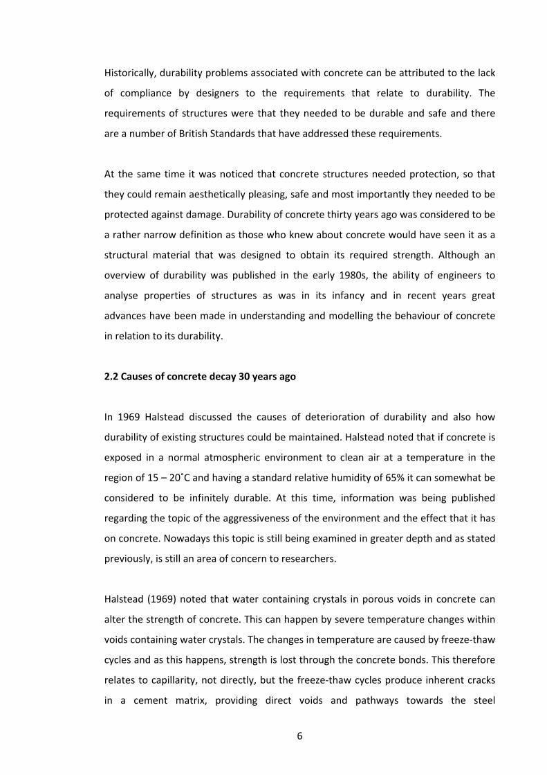
2.2 Causes of concrete decay 30 years ago 

 

In  1969  Halstead  discussed  the  causes  of  deterioration  of  durability  and  also  how 

durability of existing structures could be maintained. Halstead noted that if concrete is 

exposed  in  a normal  atmospheric environment  to  clean  air  at  a  temperature  in  the 

region of 15 – 20˚C and having a standard relative humidity of 65% it can somewhat be 

considered  to  be  infinitely  durable.  At  this  time,  information  was  being  published 

regarding the topic of the aggressiveness of the environment and the effect that it has 

on concrete. Nowadays this topic is still being examined in greater depth and as stated 

previously, is still an area of concern to researchers. 

 

Halstead  (1969) noted  that water containing crystals  in porous voids  in concrete can 

alter the strength of concrete. This can happen by severe temperature changes within 

voids containing water crystals. The changes in temperature are caused by freeze‐thaw 

cycles and as this happens, strength is lost through the concrete bonds. This therefore 

relates to capillarity, not directly, but the freeze‐thaw cycles produce  inherent cracks 

in  a  cement  matrix,  providing  direct  voids  and  pathways  towards  the  steel 

  7

reinforcement. Halstead  (1969) did not  further his studies; he only  looked directly at 

what happens to a cement matrix through freeze‐thaw cycles. Therefore, an opening 

for  future work was  created  by where  the  effect  of  ion  flow  through  cementitious 

materials subsequent to freeze‐thaw cycles could be studied, and this has been looked 

at in detail in the last 40 years.  

2.3 Carbonation of concrete  

 

Although  concrete  specimens may be  cured properly,  if exposed  to  the atmosphere 

many  changes  in  the matrix  can  happen which  can  severely  affect  their  structural 

integrity. 

 

Erlin and Hine (2004) provides a well rounded theory of carbonation. When concrete 

surfaces are  in contact with air, solid compounds react together and carbonic acid  is 

produced  from  the  reaction of carbon dioxide dissolving  in water. This acid must be 

prevented  from  being  produced  as  when  the  calcium  compounds  contained  in 

cementitious materials  react with carbonic acid,  the by product  is  silica and alumina 

gels. Carbonation produces  chemical  reactions between  carbon dioxide  from  the air 

and products from cement hydration cause reduction in alkalinity of the concrete and 

as this happens, levels of steel protection are reduced. 

 Although concrete actually increases in strength, the passive protection to steel is lost 

as alkalinity drops. 

         +     

 Figure 1: Process of carbonation through cementitious materials – based on literature 

from Erlin and Hine (2004). 

Carbon dioxide CO2 

Water H2O 

Calcium compounds 

Alumina gel 

Silica gel 

High alkalinity 

  8

Steffens (2002) created a numerical model to assess carbonation to predict corrosion 

risk  of  steel  in  concrete  structures.  At  this  period  in  time  researchers  felt  that 

information on how carbonation affects structural integrity was lacking. They note that 

concrete itself is a porous compound material consisting of mineral aggregates and the 

cement matrix that form a durable structure. They studied the porosity of the concrete 

and also noted that it provides further possible movement and retention of water and 

other substances.  

 

Their  model  uses  finite  element  analysis  alongside  their  experimental  findings  to 

assess  how  temperature, moisture  and  carbon  dioxide move  through  cementitious 

materials and  initiate  the process of  carbonation. Using  the  laws of diffusion a new 

mathematical model was created and successfully represents how moisture  is stored 

in voids in cementitious materials.  

 

Most  parameters  and  variables were  covered  experimentally  to  provide  an  overall 

model  including the change  in atmosphere  looking at the change  in temperature and 

humidity and how it affects structures. Their work does not directly focus on capillarity 

or movement of fluid through a network of voids, it only focuses on the deterioration 

properties  of  concrete  due  to moisture movement  through  cementitious materials. 

Their work could potentially be developed further if they had a better idea of different 

types of capillaries or voids in cementitious materials. 

 

Song  et  al.  (2006)  performed  experiments  to  try  and  examine  how  carbonation  of 

concrete  structures  can  be  prevented,  as  this  is  the  main  accelerator  for  steel 

corrosion and deterioration of  concrete  structures. The  review of Song et al.’s work 

(2006)  states  that  it  is  necessary  to  control  the  cracking  of  structures  to  try  and 

determine  an  evaluation  of  crack  resistance  for  structures  in  early  ages.  This  is 

something which  is hard to do as even when concrete cures and hydrates, cracks are 

produced  and  these  cracks  provide  a  direct  path  for  carbon  dioxide  to  enter  and 

therefore the process of carbonation is accelerated. 

 

  9

The  study  completed  by  Song  et  al.  (2006)  looks  at  experimental  and  analytical 

techniques  to  predict  carbonation  in  early  aged  cracked  concrete  as  they  identified 

that this is the main reason for depletion of concrete structures. Areas where there are 

high industrial fumes being produced, induce environmental pollution containing high 

amounts of carbon dioxide and  therefore additional care must be  taken  in designing 

concrete for such applications and situations. This is significant as it demonstrates the 

necessity  to  have  an  understanding  of  the  role  of  capillary  flow  in  cementitious 

materials. 

 

Carbon dioxide diffusion of pore water  in  sound concrete and cracked concrete was 

analysed by Song et al. Using equations of diffusion and with the use of finite element 

analysis characteristics of diffusivity on the carbonation of early age cracked concrete 

was used to predict the carbonation depth in pre‐cracked concrete.  

 

Song et  al.  (2006) were  successful  in  their  findings especially when  specimens were 

tested at a premature age, this was due to their ability to use finite element analysis 

models  along  with  multi  component  hydration  models  to  handle  the  diffusion  of 

carbon dioxide  in concrete. An extra addition to their model was that the model was 

able to handle extra features of  ‘real‐life’ situations such as degree of saturation and 

temperature  effects.  Modelling  saturation  directly  relates  to  the  phenomenon  of 

capillarity and there is the potential to further develop their model by seeing how the 

finite element model can relate capillarity as it does to saturation. 

 

2.4 Permeability of concrete 

 

Song et al.  (2007)  took a step  forward  into  looking at  the capillary pore structure of 

carbonated  concrete  specimens.  Unlike  previously,  their  findings  create  a more  in‐

depth analysis of what happens to a cement matrix when  it comes  into contact with 

the atmosphere.  

 

It  is  stated  that  the  rate  of  carbonation  depends  entirely  on  the  void  ratio  of  a 

structure and the moisture content of a structure, especially  in foundation structures 

  10

such  as  piles  where  the  base  of  the  structure  could  be  exposed  to  wet  soil  or 

underground water. This is a limitation in their work as in practice the aggregates will 

contribute to permeability. 

     

Figure 2: Flow of water through porous media Song et al. (2007) 

 

Song et al. (2007) completed a model to determine permeability to assess the capillary 

pore structure  in carbonated cement mortar. Assumptions taken  into their model are 

that the aggregates do not affect carbonation processes in early aged concrete. 

 

Figure 2 shows the model that they used to determine water flow  in pores  in mortar 

specimens.  It  is  a  clear  concise  way  to  show  the  flow  through  the  specimens. 

Permeability  was  measured  from  models  undertaken  looking  scales  of  a  small 

magnitude  (micrometres)  and  was  verified  with  results  from  an  accelerated 

carbonation  test  and  a  water  penetration  test  in  cement  mortar.  This  particular 

property of cementitious materials potentially defines the resistance to carbonation of 

structures. With a less permeable matrix, ions such as carbon dioxide passing through 

the concrete matrix will be less successful in simulation of moisture transfer.  

 

With work  based  in  the  lab  and  in  field  studies  assessing  carbonation  a model was 

produced  which  can  not  only  assess  structures  in  the  atmosphere  but  also  those 

underground.  Although,  it  is  evident  that  even  though  they  have  looked  into 

permeability via models using carbonation, they have not considered a range of fluids 

that could flow through a cement matrix and hence this  is a research area that could 

be developed. 

  11

 

Stated  above  in  the work  of  Song  et  al.  (2007)  it  is  important  to  have  an  idea  of 

permeability  through  concrete.  Gardner  et  al.  (2008)  completed  experimental  and 

numerical work of gas flow characteristics through concrete. 

 

Tests were performed with the use of a pressure cell apparatus, to monitor nitrogen 

gas  flow  through  concrete. Most  experimental work  previously  has  been  assessing 

water flow through cementitious materials; as such tests provide accurate measures of 

permeability as they investigate the time to reach steady state flow and also the long 

term  response of  the experimental  system. However,  they can be  timely  to prepare 

and  run. The permeability calculated  from experimental work using gas permeability 

measurements  has  both  values  and  variations  consistent  with  those  from  other 

investigations.  

 

All  of  the  work  undertaken  in  this  study  was  executed  to  look  at  cementitious 

materials  long‐term performance and durability. Many day to day processes when  in 

contact with cement based structures, such as  landfill sites with  the use of concrete 

barrier structures, accurate modelling of  fluid  flow  through cementitious materials  is 

essential. 

 

Gardner et al. (2008) discovered that permeability increases rapidly with a reduction in 

moisture  content. Data  found  in  the  literature was  obtained  for  concrete  in which 

moisture had been removed by heating. A large range of parameters were investigated 

including measurement of the connectivity of a range of pore sizes but not  individual 

pores and  capillaries. However, permeability measurements of  saturated  specimens, 

as well as specimens  less than 28 days old are still  lacking  in the  literature. These are 

areas which if discovered would provide another step towards a full understanding of 

fluid flow through cementitious materials.  

 

 

 

 

  12

2.5 Corrosion of concrete 

 

Corrosion  of  steel  reinforcement  is  known  as  a  major  cause  of  degradation  of 

reinforced  concrete  structures.  Therefore  looking  at  properties  of  flow  through 

concrete can directly relate to flow of harmful ions through concrete which affect the 

serviceability and life of concrete structures. 

 

Work by Vidal et al. (2007) assesses the predicted time taken for different fluids or ions 

to reach a specific location in discrete cracks in a beam of 17 years old. 36 reinforced 

concrete beams (300×28×15cm), were cast and then stored in a chloride environment 

under service load to take into account the influence of the flexural cracks.  

 

Results  and  readings of  chloride  flow  through  the  induced  cracks of  less  than  4mm 

showed  that  they  do  not  influence  significantly  the  corrosion  process  of  tension 

reinforcing bars and  then  the  service  life of  the  structure. However,  the bleeding of 

chloride  ions  through  the  smaller  cracks  in  concrete  was  a  cause  of  interface  de‐

bonding which could lead to early corrosion in the reinforcement. 

 

Vidal et al.  (2007) could have studied a  larger range of crack apertures through their 

specimens.  It has been  stated  that  fluid  flow  through  the  cement matrix  is  a  larger 

cause  of  corrosion  than  direct  flow  through  the  induced  cracks.  Studies  through 

smaller cracks could have benefited their work to see if smaller cracks affect corrosion. 

 

Cabrera  (1996)  has  used  numerical  models  to  assess  losses  in  serviceability  of 

reinforced concrete specimens. Data recorded  in the  laboratory was collected to  look 

at  the  rate  of  corrosion  and  was  used  in  the  numerical  models  and  against  the 

numerical model  looking at  issues of serviceability of cementitious materials, such as 

the strength of concrete after corrosion.  

 

His models were developed  further  to not only  look at  loss of  serviceability  through 

corrosion but also look at the rate of corrosion from the width and intensity of cracking 

and the bond stress through corrosion rate. Models to determine the rate of cracking 

  13

due to loss of bond strength were completed. However, no work was done to look at 

the  flow  rates of  ions  through  the cracks generated. Yet again  this suggests  that  ion 

flow  through cracks  in cementitious materials  is an area which could be  investigated 

further. 

 

Granju and Balouch (2005) focus on corrosion attack of steel fibre reinforced concrete 

(SFRC.) The effect that the steel fibres have on the cement matrix is looked at in large 

detail.  It was a concern  that  the steel  fibres could be weakened by corrosion, or  the 

opposite, they could burst the cement matrix by swelling and cracking the matrix.  

 

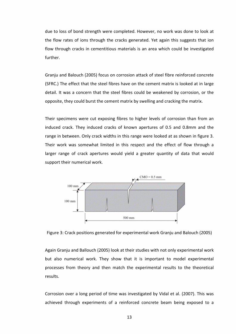
Their  specimens were cut exposing  fibres  to higher  levels of corrosion  than  from an 

induced  crack.  They  induced  cracks  of  known  apertures  of  0.5  and  0.8mm  and  the 

range in between. Only crack widths in this range were looked at as shown in figure 3. 

Their work was  somewhat  limited  in  this  respect  and  the  effect  of  flow  through  a 

larger  range  of  crack  apertures would  yield  a  greater  quantity  of  data  that would 

support their numerical work. 

 

Figure 3: Crack positions generated for experimental work Granju and Balouch (2005) 

 

Again Granju and Ballouch (2005) look at their studies with not only experimental work 

but  also  numerical  work.  They  show  that  it  is  important  to  model  experimental 

processes  from  theory  and  then match  the  experimental  results  to  the  theoretical 

results. 

 

Corrosion over a  long period of time was  investigated by Vidal et al. (2007). This was 

achieved  through  experiments  of  a  reinforced  concrete  beam  being  exposed  to  a 

  14

chloride  environment.  Their  experiments  show  that  the  bleeding  of  chloride  ions 

through  concrete  is  an  important  cause  of  deterioration  and  that  corrosion  occurs 

earlier in the compressive section of the beam. Capillarity was not mentioned directly 

although  their  conclusions  stated  that  the  crack  widths  less  than  0.4mm  do  not 

influence corrosion process directly. 

 

2.6 Chloride attack 

 

As previously discussed in section 2.1 chloride  ion attack  is one of the main causes of 

concrete deterioration and steel  reinforcement corrosion. The  literature discussed  in 

this section  look at chloride  ion  ingress  into many different types of specimens whilst 

looking at the key method of transportation of  ions through cement matrices due to 

capillarity. 

 

Azari et al.  (1993) used microsilica concrete  to determine chloride  ingress and water 

absorption  into  the  cement  matrix.  Looking  at  flow  of  ions  through  microsilica 

concrete  is  an  aspect  that  demonstrates  flow  properties  and  interaction  between 

healing agents and  ions  that  severely affect  concrete  serviceability. Determining  the 

absorption and  flow  rate of water  ions  into concrete specimens  relates  to capillarity 

such that certain flow properties can be deduced. 

 

Results  from  experimental  studies  showed  that  a  mathematical  relationship  is 

apparent between the chloride concentration and the changes  in microsilica content. 

Flow  of  chloride  ions  through microsilica  concrete  are  reactive  at  low  quantities  of 

microsilica in the specimens. Water absorption is another area that was investigated as 

flow of water was modelled through microsilica concrete. They looked at the effect of 

high water contents and lower water contents of microsilica concrete. Results showed 

that water absorption in low quantities of microsilica in concrete was more prominent 

in comparison with high quantities of microsilica in concrete. Although the results and 

readings  reflected  the water  absorption  in microsilica  concrete,  no work was  done 

looking at the effects of water absorption in concrete without microsilica. Therefore a 

  15

comparison was  not made  between  the  two  different  composites,  and  a  complete 

analysis on flow through different types of cementitious materials was not presented. 

 

Studies completed by Gowripalan et al. (2000) focus on the flow of ions in pre‐cracked 

beams. Gowripalan et al. used reinforced concrete beams that were cracked in known 

places with known crack widths. Using a 3 point bending tests the beams were loaded 

until  the desired crack width was achieved. They were  then submerged  in a chloride 

ion solution and chloride  ion profiling was used  to determine  the  rates at which  the 

ions reached the steel reinforcement. 

 

Flow  of  ions  through  cracked  specimens  was  considered  through  setting  exact 

locations where two sample holes were dry drilled and powdered samples from taken 

from  these  locations  and  the  chloride  content was  determined.  Their  studies were 

successful  in  that  they discovered how  to model and determine  the  flow of chloride 

ions through cracked specimens however; they did not determine the rate of flow of 

other  fluids  through  pre‐cracked  specimens.  Yet  again,  this  illustrates  an  area  of 

research for future investigation. 

 

Corrosion of steel reinforcement  in concrete due to transportation of chloride  ions  in 

concrete  structures  in  a  marine  environment  has  received  increasing  attention  in 

recent  years  due  to  the  high  cost  of  repair.  Song  et  al.  (2008)  examined  concrete 

specimens subjected to marine environments. They look and review previous work on 

chloride transportation by means of diffusion of concrete structures exposed to these 

environments.  Their  findings  show  that  exposure  to  sea  water  does  not  have  a 

relationship with  the  chloride  content  contained  in  the  surface of  the  structure and 

higher chloride content was found places where the cement had not been cured.  

 

However,  they  do  not  take  into  consideration  the  flow  of  ions  through  voids  and 

capillaries formed in concrete specimens. Their work solely looks at the effect of how 

the ions have penetrated the cracks in the specimens used. 

 

 

  16

2.7 Capillarity 

2.7.1 Introduction to capillary action 

 

Capillary action can be summarised by the tendency of a liquid to be drawn into a pore 

or a  small opening. Many  studies have  looked at  the  theory of  capillary  flow. These 

studies have shown how capillary flow can be applied to many different processes that 

occur  in  the  world  today.  For  instance  flow  through  soils  and  flow  through  other 

porous media.  

 

Capillary  action  in  this  study  is  considered  in  the  context  of  self‐healing  concrete, 

whereby  its  role  in  the  transport  of moisture  of  healing  agents  to  sites  of  damage 

within a cementitious material is crucial for healing to occur.  

 

For many years capillary action has been considered to be a fundamental process in a 

number of applications, as noted previously. However, capillary action in concrete has 

received little research attention since the 1970s. (Halstead, 1971). Recent research in 

concrete  structures  has  shown  that  flow  properties  such  as  permeability,  sorption, 

absorption  and adsorption of  concrete play a  significant  role  in  the deterioration of 

structures  and  the need  to ensure  the  longevity of  structures  is one of  the primary 

aims in the development of self healing concretes. 

 

2.7.2 Surface tension, cohesion and adhesion 

Cohesion  is the attractive force that acts between  liquid molecules and  is responsible 

for  the  formation of drops of water. Adhesion  is  the  force of dissimilar particles and 

surfaces  to  attract  to  one  another  (cohesion  refers  to  the  tendency  of  similar  or 

identical particles/surfaces to cling to one another). 

Surface  tension  γ,  is  a property of  the  surface of  a  liquid  that  allows  it  to  resist  an 

external force. Objects that are dense allow other liquids to be supported on the fluid 

surface.  This  is  a  key  point  when  identifying  certain  flow  properties  (Martys  and 

Ferraris 1997). 

  17

 

Fluid  flow  through  any  medium  can  also  be  altered  by  another  force,  adhesion. 

Adhesion  is  the  force  that  causes  a  fluid  to  adhere  to  the  surface  to which  it  is  in 

contact. When the cohesive force of the fluid is lower than the adhesion, the fluid will 

curve upward on the edge of the boundary as shown  in figure 4 (a). This curvature  is 

more commonly known as the meniscus. Alternatively, when the cohesive  forces are 

greater than the adhesive, the fluid will curve down at the boundary, shown in figure 4 

(b). 

 

   

         (a)                   (b) 

Figure 4: a) Cohesion forces are less than adhesion & b) Adhesion forces are greater than cohesion 

 

A combination of cohesion and adhesion causes the phenomenon known as capillary 

flow or capillarity. Without these two forces, the phenomenon of capillarity would not 

occur. A change in pressure results from changes in forces in a void or a tube caused by 

adhesion and this causes the fluid to rise upward in the void/tube. (Martys and Ferraris 

1997). 

 

2.7.3 Sorptivity 

Previous  reviews on  literature  stated above have  stated  that  cementitious materials 

are  porous.  (Gowripalan  et  al  2000)  These  pores  and  void  spaces within  a  cement 

Water in a glass tube demonstrating adhesion 

Mercury in a glass tube demonstrating cohesion 

  18

matrix either  contain  liquid or  gas. Porosity  is  recorded  as  a  ratio of  the  volume of 

voids to the total volume of material and is normally represented as a percentage.  

Concrete and cementitious materials form pore and void matrices and networks which 

connect together  in random ways. This has been demonstrated previously by Song et 

al.  (2007)  shown  in  figure  2.  Pores  can  be  completely  isolated,  such  as  small  single 

nodes  or  a  linked  network  that  leads  nowhere.  A  pore  structure  in  a  cementitious 

material cannot be modelled as they never form  in the same way and therefore only 

random generations of microstructure can be obtained. 

However, permeability of cementitious materials  is  the  flow of  fluids under pressure 

and is a function of the flow paths that create a route from face to face or surface to 

surface of the material. These can be direct paths through linked pores and capillaries, 

direct  routes  through macro‐fractures  or  slow  and  tortuous  routes  through  one  or 

combinations of many means of transport. (Marshall 1990)  

 

Sorption acts as part of the diffusion process where fluids and solutes distribute within 

a material but no fluid flow through the media is incurred by it. 

 

To  get  accurate  estimations  and  predictions  on  transport  through  the  permeable 

matrix of cementitious materials it is necessary to understand the internal structure.  

 

Whilst porosity is the measure of void space by volume and permeability the measure of 

fluid flow through or into the material, sorption is the uptake of water into a permeable 

porous  structure  through  capillary  action.  Sorption  acts without  a  pressure  head  but 

through  the  capillary  process  described  by Marshall  (1990)  and  acts  only  in  a  dry  or 

partially dry pore network. 

 

The water uptake in a material is dependent upon its coefficient of sorptivity, S, in grams 

per millimetre2  (of  the wetted area) per root time  (g/mm2∙min0.5). Equation 2.1 shows 

the relationship between sorptivity, absorption and time (Martys and Ferraris 1997):  

 

  19

i=S√t          (2.1) 

 

where:   

i = the water absorption  in g/mm2 representing the mass  increase of the sample per 

unit area of the wetted perimeter 

t = the time elapsed in minutes representing how long the sample has been in contact 

with the water. 

 

Neville  gives  typical  values  for  the  coefficient  of  sorptivity  for  concretes  with 

water/cement  ratios  of  0.4  and  0.6  as  0.09  g/mm2/min0.5  and  0.17  g/mm2/min0.5 

respectively. (Neville 1999) 

 

Roels  et  al.  (2003)  found  apertures  in  cementitious materials  and  their  surrounding 

matrices,  this was completed by a  series of experiments. Larger models  showed  the 

difference between the matrix porosity and the fracture porosity. This was found to be 

that they both contain hydraulic properties although connect to one another through 

pressure and mass.  

 

Roels et al. (2003) has provided research with a larger understanding of fluid flow with 

experiments which identify that a fractured medium is “characterised as a network of 

flow channels in which saturated flow is described using the Poiseuille equation.” Later 

experiments  relating  to  this  equation  for  laminar,  continuous  fluid  flow  through  a 

uniform  straight  pipe,  the  flow  rate  (volume  per  unit  time)  is  given  by  Poiseuille's 

Equation.  

 

X‐Ray  diffraction  was  used  by  Roels  et  al.  (2003).  Roels  et  al.  used  1D  numerical 

simulations looking at fluid flow. These simulations were used to assist further studies 

of  liquid  flow  through  cracks  in cementitious materials. Roels et al. noticed  that  the 

waterfront  in  the  fracture  quickly  reaches  the  opposite  side  of  the  specimen  as 

absorption occurs  through  the surrounding matrix with  the use of crack apertures  in 

the region of 0.1mm. 

 

  20

2.7.4 Equation of capillarity 

 

The  Lucas‐Washburn  equation  was  developed  in  1921.  Washburn  undertook  a 

theoretical  investigation  in which he considered the effects of the capillary force and 

viscous drag on circular capillaries and porous bodies. Lucas‐Washburn’s equation was 

fundamental to developing understanding of capillary flow. 

 

The  Lucas‐Washburn equation  is  considered  in more detail  in Chapter 5 by where a 

numerical simulation of flow equation is analysed for capillaries. 

Analytical modelling of liquid rise in a capillary tube has been investigated thoroughly 

by  Liou  et  al.  (2009) with  various  fluid models.  They  start  from  the original Navier‐

Stokes  equations  which  represent  incompressible  fluid  flow  in  capillaries  which  is 

written as; 

uPuutu 2. ∇+

∇−=∇⋅+

∂∂ ν

ρ         (2.2) 

Where:   ‐ is the kinematic viscosity, Ns/m2 

               ‐ is the velocity of the fluid parcel, m/s2 

               ‐ is the fluid‐pressure, N/m 

              ‐ is the fluid density. kg/m2 

From  this  equation  Liou  et  al.  (2009)  derive  a model  for  time  dependant  interface 

capillary rise.  

 

 

  21

 

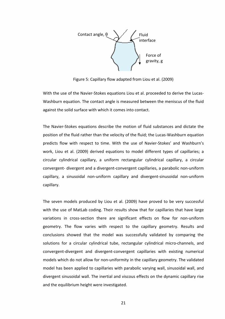
Figure 5: Capillary flow adapted from Liou et al. (2009)  

With the use of the Navier‐Stokes equations Liou et al. proceeded to derive the Lucas‐ 

Washburn equation. The contact angle is measured between the meniscus of the fluid 

against the solid surface with which it comes into contact. 

 

The Navier‐Stokes equations describe  the motion of  fluid substances and dictate  the 

position of the fluid rather than the velocity of the fluid; the Lucas‐Washburn equation 

predicts  flow with  respect  to  time. With  the  use  of Navier‐Stokes’  and Washburn’s 

work,  Liou  et  al.  (2009)  derived  equations  to model  different  types  of  capillaries;  a 

circular  cylindrical  capillary,  a  uniform  rectangular  cylindrical  capillary,  a  circular 

convergent‐ divergent and a divergent‐convergent capillaries, a parabolic non‐uniform 

capillary,  a  sinusoidal  non‐uniform  capillary  and  divergent‐sinusoidal  non‐uniform 

capillary.  

 

The  seven models produced by  Liou et al.  (2009) have proved  to be very  successful 

with the use of MatLab coding. Their results show that for capillaries that have  large 

variations  in  cross‐section  there  are  significant  effects  on  flow  for  non‐uniform 

geometry.  The  flow  varies  with  respect  to  the  capillary  geometry.  Results  and 

conclusions  showed  that  the  model  was  successfully  validated  by  comparing  the 

solutions  for  a  circular  cylindrical  tube,  rectangular  cylindrical micro‐channels,  and 

convergent‐divergent  and  divergent‐convergent  capillaries  with  existing  numerical 

models which do not allow for non‐uniformity in the capillary geometry. The validated 

model has been applied to capillaries with parabolic varying wall, sinusoidal wall, and 

divergent sinusoidal wall. The inertial and viscous effects on the dynamic capillary rise 

and the equilibrium height were investigated.  

Fluid interface 

Force of gravity, g 

Contact angle, θ 

  22

Stevens  et  al.  (2009)  take  the  work  of  Bahramian  and  Danesh  (2004)  to measure 

contact  angles  from  capillary pressure measurements  from packed beds of particles 

which are partially saturated with liquids.  

 

Zhmud  et  al.  (2000)  examined  the  analysis  of  the  original  theory  of  capillarity. 

Experimental work  and numerical work was performed by  the  researchers  to  try  to 

capture the phenomenon of capillary rise. Capillary rise was measured with the use of 

borosilicate  glass  capillaries with  radii of  0.1,  0.15,  0.25  and  0.5mm  and  the  liquids 

used  in  experimentation were  surfactant  solutions,  such  as  ethoxylated  trisiloxiane, 

liquids with a low surface tension. These solutions were used to ensure that there was 

no  interference between  the  fluid and  the  capillaries. The dynamics of  capillary  rise 

was captured as soon as the liquid was put in contact with the capillary. The capillary 

rise was recorded with the use of high speed camera software. One‐thousand frames a 

second were recorded to assess the phenomenon of capillary flow. However, a limited 

number of glass capillaries over a relatively small size range were used. The range of 

fluids was also  limited as only  two  surfactants were used and other  fluids with high 

surface tension were not used.  

Funada and Joseph (2002) created a numerical tool to model the instability of capillary 

flow in a viscous tube. The phenomenon of their model is shown below in figure 6.  

 

 

 

 

 

 

 

Figure 6: Adapted from Funada and Joseph (2002), instability of viscous flow in a capillary 

 

Capillary forces, F causing instability 

R F 

Downwards forces acting on the capillary 

Upwards forces acting on the capillary 

  23

The model completed by Funada and Joseph (2002) model has been compared against 

the original Navier‐Stokes Equations. More updated studies by Funada and  Joseph  in 

2002 show that in a numerical form capillary instability (where the forces of a fluid in a 

capillary are not equal) of a  liquid  cylinder of mean  radius R  leads  towards  capillary 

collapse. This phenomenon of an  instable capillary  is described by Funada et al. as a 

‘neck down’ due to surface tension γ, in which fluid is injected from the throat of the 

neck,  leading  to  a  smaller neck  and  greater neck down  capillary  force,  F  as  seen  in 

figure 6. 

Theory of  instability along a  long capillary cylinder was  initially studied by Rayleigh  in 

1897 and his findings are now considered to be somewhat  inaccurate as they neglect 

the outer  fluid.  This outer  fluid  that  is  in  contact with  the outer  surface provides  a 

force  known  as  viscosity.  Rayleigh  then  developed  his methods  to  account  for  this 

viscous force, although his findings were found as  incomplete.  In  later years Fundada 

and  Joseph  (2002)  looked  at  viscous  potential  flow  analysis  and  now  the  issue  of 

capillary instability can be assessed with the use of new model by Funada and Joseph 

(2002)  in  the  fully viscous and potential  flow cases  so no  forces are neglected. They 

show that capillary instability is prominent in places where there are pressure changes. 

It is necessary to have an understanding of the different types of forces apparent in a 

capillary. Funada and  Joseph successfully show  through  their numerical work  flow of 

fluids through a capillary and how different capillaries can affect the flow rates. 

 

Viscosity is one of the key properties of a fluid and the Reynolds number represents a 

fluids  viscosity.  A  fluid’s  viscosity  is  an  important  parameter  as  it  represents  the 

property of a  fluid which  resists  the  force making  the  fluid  flow. For  instance, when 

two fluids are next to one another they do not necessarily mix. Transportation within 

the surface molecules and the fluid molecules are then transported through diffusion. 

Funada and Joseph (2002) state that is important to have an understanding about how 

a fluid’s viscosity related to diffusion as they can affect the phenomenon of capillarity.  

 

 

 

  24

2.7.5 Capillary flow and contact angles 

 

Young  (2004)  forms  a model of  the  interface progression  in  a non‐uniform  capillary 

based on analysis of the Lucas–Washburn equation.  

 

Young (2004) demonstrates the effect that capillary geometry has on the progress of 

the  interface.  A  solution  of  the  time  required  for  interface  advancement  without 

gravity  in  a  non‐uniform  capillary was  developed  using  theory  based  on  the  Lucas‐

Washburn equation. It was discovered that for capillary advancement along horizontal 

pipes without gravity,  the wetting  time was  found  to depend on some parameter of 

the capillary geometry. This model developed by Young (2004)  is used  in chapter five 

as the theory is used to model the experiments presented in chapter 3. 

 

Bahramian and Danesh. (2004) explore how to predict the solid‐vapour and solid‐liquid 

interfacial  tension with  the use of a numerical model. The necessary parameters  for 

this  to be possible are  the  liquid  critical  temperature and  volume,  the  solid melting 

temperature  and  the  volume  of  liquid  and  solid  compounds.  The  results  were 

produced  each  evaluating  the  solid‐fluid  interfacial  tension  values  to  predict  the 

contact angle of  the  liquid drop on  the  solid  surface. This was done with  the use of 

Young’s  equations  (2004).  Bahramian  and  Danesh  (2004)  were  successful  in  the 

prediction of the contact angles along side their experimental data proving that their 

models are accurate and reliable. The contact angles were measured by a microscope 

image  of  a  droplet  on  a  plate  and  the  angle  subsequently  recorded.  This  is  a  good 

method and is later shown to be developed in chapter 5 where a discussion on contact 

angles is presented. 

 

The  theory  behind  their  work  shows  that  the  difference  in  solid–liquid  and  solid–

vapour tension has a close relationship with the liquid’s surface tensions, viscosity and 

the contact angle between the liquid drop and the surface, shown in figure 7. 

 

 

 

  25

 

 

Figure 7: Fluid on solid planar surface 

 

As  all  of  these  parameters  are  either  known,  or  measureable  so  therefore  with 

different  fluids  and  the  contact  angles measured,  these  values  can  be  used  in  the 

model to determine the solid‐fluid and solid‐vapour interfacial tension.  

 

Bahramian  and  Danesh  (2004)  successfully  predicted,  via  experimental  work  and 

numerical models, the contact angles to predict the interfacial tension. Although their 

work was successful, it does not verify interfacial tension. Therefore highlights an area 

of  research  that  could  involving different  fluids  to predict  contact angles  for  certain 

fluids to be furthered. 

 

Behaviour of fluids at an infinitely small scale has been an interest throughout history 

of science and microfluidics is an area where this concept is investigated. Behaviour of 

fluids at a large (marco) scale is different to the behaviour of a fluid at a smaller scale 

as  surface  tension,  energy  dissipation  and  fluidic  resistance  start  to  dominate  the 

system. The studies that have been completed on microfluidics look at how behaviours 

change at  this  small  scale and how  they can addressed, or eliminated  for new uses. 

(Roels et al. 2003) 

 

The work completed by Roels et al. therefore relates to capillarity as it is important to 

have an understanding of how  fluids behave at certain scales. The capillaries used  in 

this thesis range from 0.094 to 1.170mm so parameters like surface tension do need to 

be taken into consideration. 

 

  26

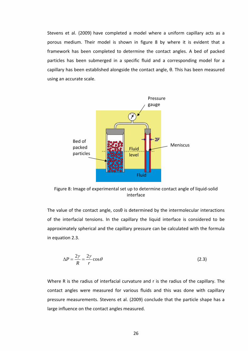
Stevens  et  al.  (2009)  have  completed  a model where  a  uniform  capillary  acts  as  a 

porous  medium.  Their  model  is  shown  in  figure  8  by  where  it  is  evident  that  a 

framework  has  been  completed  to  determine  the  contact  angles.  A  bed  of  packed 

particles  has  been  submerged  in  a  specific  fluid  and  a  corresponding model  for  a 

capillary has been established alongside the contact angle, θ. This has been measured 

using an accurate scale. 

 

 

 

 

 

 

 

 

 

 

 

Figure 8: Image of experimental set up to determine contact angle of liquid‐solid interface 

 

The value of the contact angle, cosθ  is determined by the  intermolecular  interactions 

of  the  interfacial  tensions.  In  the  capillary  the  liquid  interface  is  considered  to  be 

approximately spherical and the capillary pressure can be calculated with the formula 

in equation 2.3.  

   

θγγ cos22rR

P ==Δ               (2.3) 

 

Where R  is the radius of  interfacial curvature and r  is the radius of the capillary. The 

contact  angles  were measured  for  various  fluids  and  this  was  done  with  capillary 

pressure measurements. Stevens et al.  (2009) conclude that the particle shape has a 

large influence on the contact angles measured. 

 

Fluid 

Bed of packed particles 

Fluid  level 

Meniscus 

Pressure gauge 

  27

Hanzic  et  al.  (2010)  state  that  it  is  hard  to  determine  the  difference of  the  contact 

angle between the fluid and the concrete wall. It is also shown that at a nano‐scale the 

contact angle changes so much more when it is in contact with the capillary wall. This 

is due to the roughness of the wall.

2.7.6 Capillarity and cementitious materials

 

Gospodinov (2005)  looks at the phenomenon of diffusion and  in this case diffusion of 

sulphate ions into cementitious materials. The other areas also looked at in detail are 

microcapillary  filling  and  the  following  liquid  push  out  of  capillaries.  He  created  a 

numerical model and looked at an in‐depth view of ion diffusion through cementitious 

materials. He then compared the results with experimental observations of corrosion 

processes  in  concrete.  Experimental  work  and  numerical  studies  explored  by 

Gospodinov  (2005)  include  the  diffusion  of  ions  in  saturated  and  nonsaturated 

concrete  systems.  Studies were also  completed on  the effects of environments  that 

are  particularly  aggressive  and  contain  large  quantities  of  ions  that  degrade 

cementitious  materials.  The  conclusions  drawn  through  the  experimental  work 

conclude that the movement of the ions throughout the concrete matrix can only flow 

in the  liquid phase. Therefore the movement of  ions through a concrete matrix move 

due  to diffusion. Tests  that  identify migration and diffusion of  ions  through concrete 

were  also  conducted;  these  were  used  to  provide  an  estimation  of  the  diffusion 

coefficients  of  the  cementitious  materials  used.  From  the  results  and  simulations 

discussed  in  Gospodinov’s work,  real  transfer  conditions  of  ions  through  a  cement 

matrix could be simulated. The numerical algorithm looked at solutions to differential 

equations  to  simulate  liquid push out by where  ions are  removed  from one pore  to 

another in situations in structures.  

Lepech  and  Li  (2009)  researched  the water  permeability of  high  performance  fibre‐

reinforced  cementitious  composites  of  HPFRCC.  Again,  experimental  work  was 

undertaken  and  compared  with  a  numerical  model.  As  the  specimens  of  HPFRCC 

undergo  tensile  deformation  cracks  are  formed. Microcracking was  the  key  area  of 

observation as the authors did not want the micro cracks to develop into larger cracks. 

  28

The micro‐cracks  formed were  in  the  region  of  approximately  60  μm  in width.  The 

cracks were  then  saturated  in a  chloride  ion  solution and using micromechanics  the 

theoretical basis  for tailoring materials  for tight crack width and correspondingly  low 

permeability was  established.  Tests were  then  used  after  to  determine  if  the  new 

materials HPFRCC could maintain tight crack widths under tensile strain. Lepech and Li 

(2009) were successful  in that they established models and results  for  flow  in micro‐

cracks of HPFRCC concrete, however they only examined one crack aperture and their 

work may have been improved by looking at a larger range of crack apertures.  

A  study  by  Hoffman  (2009)  focussed  on  capillary  flow  and  looked  directly  at 

experimental and numerical studies of capillary  flow simulated  through a number of 

experimental methods  that  analysed  different  capillary  rise  heights with  respect  to 

different  crack  apertures.  The  general  trend  in  the  readings  showed  that  as  crack 

aperture increased over a time period of three minutes the final rise height decreased. 

The  theory  behind  this  phenomenon  is  due  to  the  surface  tension  and  viscosity 

parameters  relating  to  the equation  governing  capillary  action which  is explained  in 

depth in chapter 5 of this thesis.  

 

A  limitation  of  this work  is  that  the  author  only  looked  at  fluid  flow  in  cracks  at  a 

period of time greater than 10 seconds. This thesis takes a step forward and  looks at 

the crack aperture with  respect  to  rise height within 6 seconds and  flow  is captured 

using high‐speed cameras.  

 

2.7.7 Kinetics of capillary absorption 

 

Fluid flow through a cement matrix occurs in voids. This happens as diffusion, suction 

and  capillary  absorption  force  the  fluid  through  the  matrix.  Diffusion  and  suction 

happens while  there  is a change  in  the pressure gradient of gas and  fluids. Capillary 

flow and absorption is different as it is altered by surface tension and surface tension 

changes depending on the fluid used or the surface with which it is in contact. 

 

  29

Hanzic et al. (2010) explore the kinetics of capillary absorption; this is done by creating 

experiments to find a capillary coefficient for a concrete matrix. Transport of liquids in 

porous media  such  as  concrete  takes  place  in  open  pores mainly  due  to  diffusion, 

suction and capillary absorption. 

 

With the use of calculated capillary coefficients through experimental work; the  flow 

and  kinetics  of  fluids  through  cement  matrices  was  studied  in  depth.  Studies 

completed by Hanzic et al.  (2010) used ethylene glycol  to  look  in depth at  concrete 

matrix porosity and liquid viscosity. Ethylene‐glycol is the fluid chosen to complete the 

experimental work as  it  is a  fluid which does not  react with  cement gel. Hence,  the 

flow  of  fluid  can  be  modelled  using  Neutron  radiography,  and  their  results 

demonstrated capillary flow through cementitious materials. For the determination of 

capillarity  with  the  use  of  neutron  radiography  the  height  of  the  liquid  front  was 

measured  in  three  vertical profiles either by measuring  the distance directly on  the 

digital neutronograph.  

 

The  experiments  were  completed  to  study  reasoning  for  capillary  flow  of  water 

through concrete with use of the Lucas‐ Washburn equation. Hanzic et al. (2010) show 

that the Lucas‐Washburn equation is only valid for up to 25 hours. This implicates that 

swelling and rehydration within the cement‐matrix  is not a valid reason for deviation 

of  the  capillary  coefficient  in  the  concrete‐water  experimental work.  Therefore  this 

experiment is not suitable for long term applications, greater than 25 hours.  

Through  experimental  work  Hanzic  et  al.  (2010)  concluded  many  reasons  behind 

capillary flow: 

 

• Diffusion  through  the  cement matrix  is  very  low  and  is  found  to  be  a  rare 

phenomenon  in  this  case.  This  was  found  from  their  work  on  neutron 

radiography and it is shown by movement of the molecules.  

• Suction  shows  that  liquid  is  represented  by  its  viscosity,  it  occurs  in  larger 

pores. 

 

  30

Capillary  absorption  occurs  in  small  pores  as  well  as  larger  pores,  however  the 

experimental studies focused on those  in the range from 10 nm–10 μm. In this range 

of size, the forces arising from surface tension are in the same range as gravity forces 

present in the liquid and therefore the phenomenon of capillarity is not as prominent. 

2.8 Self healing cementitious materials 

 

Self healing is of particular interest in this study as flow properties and capillarity play a 

large  part  in  the  area  of  the  ability  of  concrete  to  self‐repair.  There  are  two main 

categories  of  self  healing,  autogenic  healing  and  autonomic  healing.  These  are 

discussed in more depth below.  

 

2.8.1 Definitions 

 

Below the different types of self healing materials are discussed and how they play a 

part in cementitious materials. 

 

2.8.1.1 What are smart self healing materials? 

 

“Smart structures are engineered composites of conventional materials, which 

exhibit  sending  and  actuation  properties,  due  to  the  properties  of  the  individual 

components.” (Joseph et al. 2010) 

 

2.8.1.2 Autogenous self healing 

 

Autogeneous healing  is  the natural ability of concrete  to self  repair. There are  three 

primary mechanisms of autogenic healing. These are as the following. 

 

• When a specimen  is rehydrated, the water can react with unhydrated cement 

in the concrete matrix and repair any cracking.  

• Movement of fragments in water 

• Precipitation of calcium carbonates 

  31

 

 

2.8.1.3. Autonomic self healing 

 

Autonomic healing  is where  the  cementitious material, whether  it  is either a beam, 

slab or any other concrete composite, has been manufactured  to have  the ability  to 

self heal.  

 

The most  common  healing  agents  that  are  used  for  autonomic  healing  are  epoxy 

resins, cyanoacrylates and alkali‐silica solutions.  

2.8.2 Autogenic healing studies 

 

Recently, concrete has been discussed in further detail in many articles of progression 

of the phenomenon of self‐healing concrete. McAlpine (2010) debates the differences 

between the phenomenon of self‐healing concrete and the production of calcite with 

the  use  of  bacteria.  Previously  stated,  concrete  is  susceptible  to  deterioration  and 

Jonkers (2010) of Delft University of Technology in Delft, the Netherlands, summarizes 

the key problematic area "Water is the culprit for concrete because it enters the cracks 

and  it  brings  aggressive  chemicals with  it.” A  key  issue  is  that  it  seeps  through  the 

cement matrix and corrodes the steel. 

A  conclusion between  the  scientists was  that  they  should be  able  to  locate,  and  to 

some form  ‘seal’ the crack. Jonkers (2010), believes that healing concrete should and 

potentially can be done by using water flow as the start and by packing the concrete 

with  bacteria  that  use  water  and  calcium  lactate  "food"  to  make  calcite,  natural 

cement. 

However, concrete has a very alkaline pH of around 10 and might be higher. Calcite 

producing  organisms  cannot  survive  in  this  alkalinity.  Jonkers  and  colleagues 

discovered  natural  bacteria  known  by  Bacillus  present  in  soda  lakes  in  Russia  and 

Egypt. Another interesting fact is that these bacteria, Bacillus, can survive without any 

  32

food and spore for long periods of time, up to 50 years long. The significance of these 

bacteria  is  that  if  its by‐products can  spore  for  long periods of  time and are used  in 

healing mechanisms these will last for long periods of time. 

Their experimental work  consisted of producing  ceramic pellets  ranging  from 2  to 4 

millimetres in diameter, and adding them to the concrete mix. Preventing the bacteria 

from  activating  in  the mixture was  seen  to  be  challenging.  This was  because  they 

wanted  for  the spores  to only produce calcite when opened by microcracking  in  the 

concrete. 

When  cracking occurs  in  the  concrete,  the pellets open  and water  seeps  inside  the 

cracks. As this occurs, the bacteria feed off of the water and the embedded nutrients 

and produce calcite and carbon dioxide. Calcite is pure limestone so essentially this by 

product heals the cracks. 

In 1983 Hannant and Keer (1983) discovered the ability of autogenous healing of thin 

cement  based  sheets.  Natural  weathering  was  examined  on  pre‐cracked  fibre 

reinforced mortar. Weathering on specimens was examined for a period of up to two 

years. Results showed  that cracks will heal sufficiently under natural weathering but 

the healed cracks are unable to carry high tensile stresses. 

 

Hannant and Keer (1983) did not  look  into autogenous healing of  large crack widths, 

therefore there is a lack in their data which should be addressed in the future.  

Van Tittelboom et al. (2010) come up with a more environmentally friendly method to 

help  towards  self  healing  cementitious  materials.  They  use  a  biological  repair 

technique; Ureolytic bacteria such as Bacillus sphaericus can precipitate CaCO3 in their 

micro  environment  by  conversion  of  urea  into  ammonium  and  carbonate.  The 

precipitated  crystals  produced  by  the  bacteria  can  fill  the  cracks  produced  in  a 

concrete matrix.  

 

  33

Through experimental work the analysis showed that this type of bacteria was able to 

precipitate  CaCO3  crystals  in  the matrix  to  fill  up  and  voids  or  created  capillaries. 

However,  although  Van  Tittelboom  et  al.  (2010)  reported  some  success  in  their 

findings the results did not reflect any work on durability or serviceability of structures 

with the bacteria in concrete.  

Jefferson  et  al.  (2010)  research  into  the  smart  self  healing  field  by  looking  at  the 

potential for a crack closure system with the use of shrinkable polymer tendons. Their 

experimental work  includes unbonded pre‐oriented polymer tendons  in cementitious 

beams.  The  tendons  are  activated  through  an  increase  in  temperature  after  the 

cement based material has undergone initial curing. 

 

The system is demonstrated with the use of a series of small scale experiments of pre‐

cracked mortar specimens. Results show that upon thermal activation of the tendons, 

the tendon completely closes the macro‐cracks. Therefore this system  is successful  in 

its ability to enhance autogenous healing and improve structural durability. 

 

Qian et al.  (2009)  look at  the  self healing behaviour of  cementitious materials using 

blast  furnace slag and  limestone powder  to determine what effect  they have on  the 

recovery of a  specimen’s deflection  capacity. Four point bending  tests were used  to 

crack  the beam at 28 days. Results  showed  that beams  submerged  to water healing 

recovered strength in the region of 65‐105% which is much higher than those healed in 

air. 

 

The work completed by Qian et al. (2009) has furthered research in that their work can 

potentially reduce or even eliminate the maintenance of civil infrastructure. 

 

2.8.3 Autonomic healing studies 

 

Li et al. (1998)  initiated the feasibility of smart healing  in cementitious materials. The 

smart  materials  in  their  work  include  the  sensors  and  actuators  in  the  form  of 

controlled micro cracks and hollow glass fibres carrying air‐curing chemicals.  

  34

 

One self‐healing concept is to release chemicals which seal the tensile cracks, followed 

by  air  curing  of  the  released  chemicals  in  the  cracks,  leading  to  regaining  the 

mechanical properties of the uncracked composite. The experiments conducted in the 

studies  look  at  controlled  micro‐cracking.  Afterward,  the  effectiveness  of  the  self 

healing  is confirmed by the elastic modulus of  the composite after  it undergoes self‐

healing with  the  use  of  air  curing  chemicals.  Li  et  al.  (1998)  produced  encouraging 

results as  they  showed  that after  the  first  loading  cycle  the  composites  regain  their 

strength  and  return  to  their  original  elastic modulus.  Studies  looked  at  by  Li  et  al. 

include  those  that  look at  sealing/healing chemicals contained  in hollow brittle glass 

fibers and this work was furthered by Joseph et al. (2010)

 

Joseph  et  al.  (2010)  state  that  there  are  definite  properties  that  a  self‐healing  flow 

agent must  possess. One  of  these  is  that  it  is  necessary  to  have  a  low  viscosity  to 

ensure a wider repair area and a sufficiently strong bond between crack surfaces and 

that there should be adequate capillary forces to draw the agent into the crack. Later 

work by Joseph et al. (2010) examined in more detail studies on self healing of mortar 

beams. 

 

Figure 9 shows the concept that has been addressed through the work of Joseph et al. 

(2010)  and  the  process  of  capillary  action  that  occurs  through  cracks  induced  in 

cementitious materials via 3 point bend tests.  

 

Cyanoacrylates  that  come  into  contact  with  moisture  react  and  cure  very  rapidly 

forming a bond often stronger than the material  it  is bonding,  i.e. concrete. Figure 9 

again shows the developed system by Joseph who shows that  if a system  is damaged 

and healed and then damaged again, a new crack will form around the healed crack. 

 

Their work directly relates to the studies undertaken in this thesis. This is a successful 

model  for  autonomic  healing,  and  depending  on  the  different  types  of  crack 

propagations and  fluids, models and experiments have been  completed  to  relate  to 

determine the length of time it takes for the fluid to fill up the crack or capillary. 

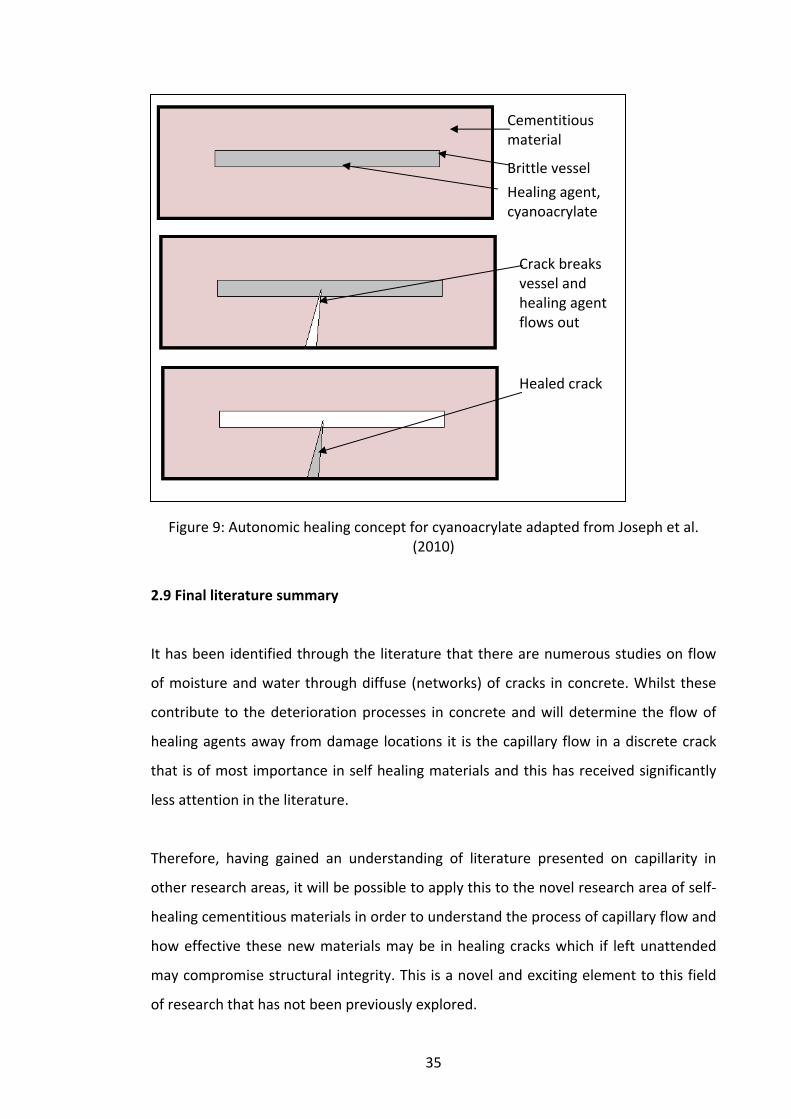
  35

 

 Figure 9: Autonomic healing concept for cyanoacrylate adapted from Joseph et al. 

(2010)  

2.9 Final literature summary 

 

It has been  identified through the  literature that there are numerous studies on flow 

of moisture and water through diffuse  (networks) of cracks  in concrete. Whilst these 

contribute  to  the deterioration processes  in concrete and will determine  the  flow of 

healing agents away from damage  locations  it  is the capillary flow  in a discrete crack 

that  is of most  importance  in self healing materials and this has received significantly 

less attention in the literature.  

 

Therefore,  having  gained  an  understanding  of  literature  presented  on  capillarity  in 

other research areas, it will be possible to apply this to the novel research area of self‐

healing cementitious materials in order to understand the process of capillary flow and 

how effective  these new materials may be  in healing cracks which  if  left unattended 

may compromise structural  integrity. This  is a novel and exciting element to this field 

of research that has not been previously explored. 

Cementitious material 

Brittle vessel 

Healing agent, cyanoacrylate 

Crack breaks vessel and healing agent flows out 

Healed crack 

36

Chapter 3 

Experimental Procedure 

 

 

 

3.1 Introduction  

Self‐healing and capillary flow through cementitious materials are two key areas that 

can  be  combined  together  to  provide  an  in‐depth  investigation  of  the  potential  for 

self‐healing  in  concrete. The  investigations  conducted  in  this  thesis assess how  fluid 

flow through capillaries, in the form of discrete cracks, can influence the rate at which 

self‐healing may occur in cementitious materials. Glass capillaries have been previously 

used in research to determine properties of capillary flow (Zhmud et al. 2000) and are 

used  in  this  experiment  to  compare  capillary  flow  in  glass  to  capillary  flow  in 

manufactured mortar  capillaries. Many  variables  including,  but  not  limited  to,  the 

characteristics  of  the  capillary  surface  and  the  nature  of  the  fluid  need  to  be 

considered such that a rigorous experimental procedure can be completed. 

 

The  experimental work  undertaken  in  this  thesis  uses mortar  specimens  and  fluids 

with varying viscosities in order to examine the effect of different crack/capillaries on 

the  rate and  level of capillary  rise height. Coarse aggregates were not used  in  these 

experiments as  it was necessary to omit the effect of the absorption of  fluids by the 

coarse aggregate during capillary rise. Moreover, it is assumed that cracks originate at 

the  aggregate‐mortar  interface  and  propagate  through  the  mortar  matrix  and 

therefore it is the flow properties of the mortar phase alone that are of most interest.  

 

 

 

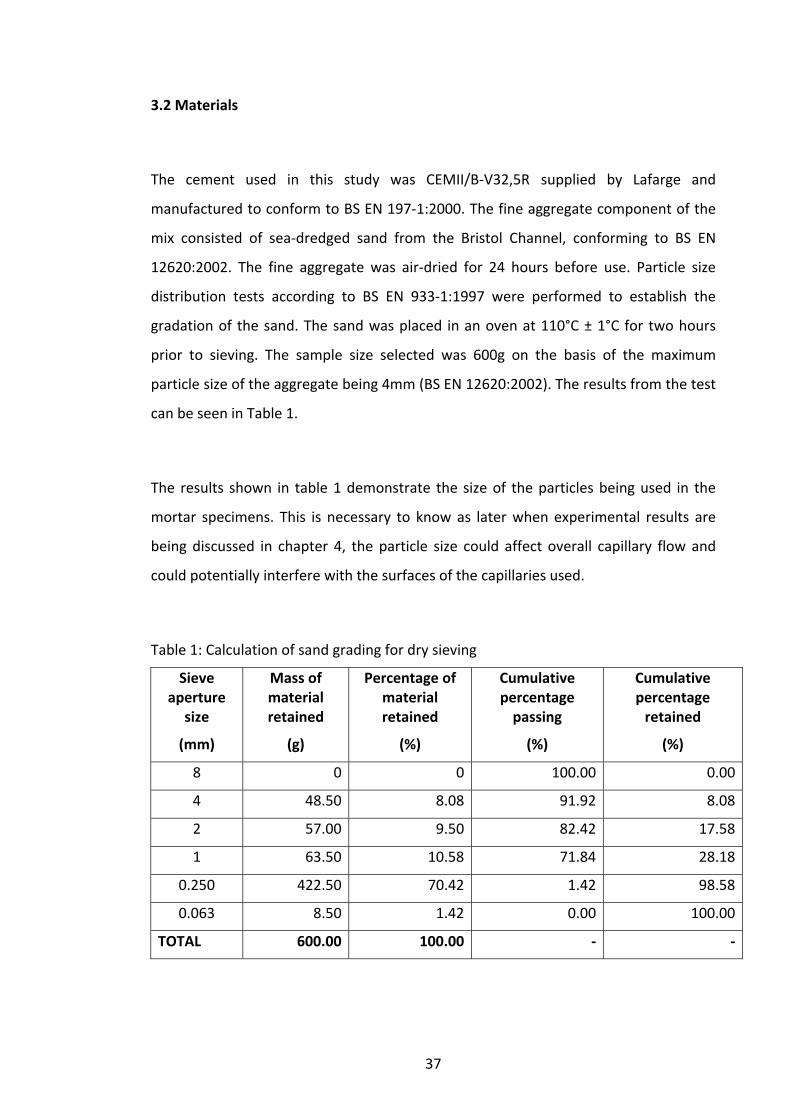
37

3.2 Materials 

 

The  cement  used  in  this  study  was  CEMII/B‐V32,5R supplied  by  Lafarge  and 

manufactured to conform to BS EN 197‐1:2000. The fine aggregate component of the 

mix  consisted  of  sea‐dredged  sand  from  the  Bristol  Channel,  conforming  to  BS  EN 

12620:2002.  The  fine  aggregate was  air‐dried  for  24  hours  before  use.  Particle  size 

distribution  tests  according  to  BS  EN  933‐1:1997  were  performed  to  establish  the 

gradation of the sand. The sand was placed  in an oven at 110°C ± 1°C  for two hours 

prior  to  sieving.  The  sample  size  selected was  600g  on  the  basis  of  the maximum 

particle size of the aggregate being 4mm (BS EN 12620:2002). The results from the test 

can be seen in Table 1.  

 

The  results shown  in  table 1 demonstrate  the size of  the particles being used  in  the 

mortar  specimens. This  is necessary  to know as  later when experimental  results are 

being discussed  in  chapter 4,  the particle  size  could affect overall  capillary  flow and 

could potentially interfere with the surfaces of the capillaries used. 

 

Table 1: Calculation of sand grading for dry sieving 

Sieve aperture 

size 

(mm) 

Mass of material retained  

(g) 

Percentage of material retained  

(%) 

Cumulative percentage passing  

(%) 

Cumulative percentage retained  

(%) 

8  0 0 100.00  0.00

4  48.50 8.08 91.92  8.08

2  57.00 9.50 82.42  17.58

1  63.50 10.58 71.84  28.18

0.250  422.50 70.42  1.42  98.58

0.063  8.50 1.42 0.00  100.00

TOTAL  600.00 100.00 ‐  ‐

 

 

38

The mix  proportions were  selected  on  the  basis  of  a  standard mortar mix  used  in 

previous  laboratory  work.  The  composition  of  the mix  was  540kg/m3:  1618kg/m3: 

242kg/m3  (cement:sand:water).  The  resulting  mortar  had  an  average  compressive 

strength of 36.7 N/mm2 and was used in each experiment.  

 

3.3 Specimen manufacture 

3.3.1 Specimen numbers and form 

Twelve  prisms  of  dimensions  255mm  x  75mm  x  75mm  were  cast  for  each  crack 

configuration experiment.  It was decided that this number of specimens would allow 

11 different crack apertures to be explored and enable sufficient specimens to be cut 

from  each  prism  to  allow  repeat  tests  to  be  conducted.  Seven  to  eight  pairs  of 

specimens (a pair comprised Specimen 1 and Specimen 2 as shown in table 2) for the 

tests  were  taken  from  each  prism  cast.  The  specimen  designation  was  selected 

depending on  the age  (old or  young),  crack  configuration  (planar,  tapered,  tortuous 

and  natural),  flow  agent  (water  or  cyanoacrylate)  and wire  thickness  in  the  range 

shown in table 2 for each of the experiments.  

 

Table 2: Specimen referencing and form 

Experiment  Specimen 1  Specimen 2  Range of crack apertures (mm) 

Old, planar, water & cyanoacrylate 

1a‐36a  1b‐36b  0.094‐1.170 

Old, tapered, water & cyanoacrylate 

2a‐22a  2b‐22b  0.094‐1.170 

Old, tortuous, water & cyanoacrylate 

t1a‐t28a  t1b‐t28b  0.094‐0.714 

Old, natural, water, with reinforcement 

t1‐t14  N/A  0.094‐1.170 

Old, natural, water, without reinforcement 

t1a‐t14a  t1b‐t14b  0.094‐1.170 

39

The  video  files,  providing  the  full  fluid  flow  history  through  the  various  crack 

configurations have been named in a similar manner and are provided on the CD‐ROM 

accompanying this thesis. Typically 3 tests were performed for each crack width for all 

crack configurations, specimen ages and degrees of saturation. An exact breakdown of 

the number of specimens tested is provided in Appendix A. 

 

3.4 Casting 

3.4.1 Mix procedure 

As previously mentioned  the mix proportions were kept consistent  throughout all of 

experiments  to  ensure  that  the  specimens  all  had  a  similar  composition.  The 

constituent materials were weighed,  in  buckets  to  an  accuracy  of  0.05kg.  The  dry 

materials were mixed together for approximately five minutes in a Cumflow horizontal 

pan mixer with a capacity of approximately 250kg. The water was then added to the 

pan  in  three  stages  using  a  visual  inspection  of  the  mix  to  achieve  a  suitable 

workability. Once fully mixed the mixture was then placed into the moulds.  

 

The moulds were filled in thirds. After each third was added the moulds were vibrated 

for 30 seconds. This process was repeated for the remaining two thirds of the moulds. 

Once all of the mortar was placed in the moulds, the tops were leveled using a pallet 

knife. 

 

3.4.2 Specimen curing 

Two curing procedures were used  to obtain old and young specimens and  these are 

described in more detail in the following sections. 

 

3.4.2.1 Curing procedure for old specimens 

After casting the specimens were left for 24 hours before being demoulded. They were 

then wrapped  in  damp  hessian  for  14  days  and  covered  in  plastic  so  the moisture 

content was kept constant. Every two days the hessian was re‐soaked to prevent the 

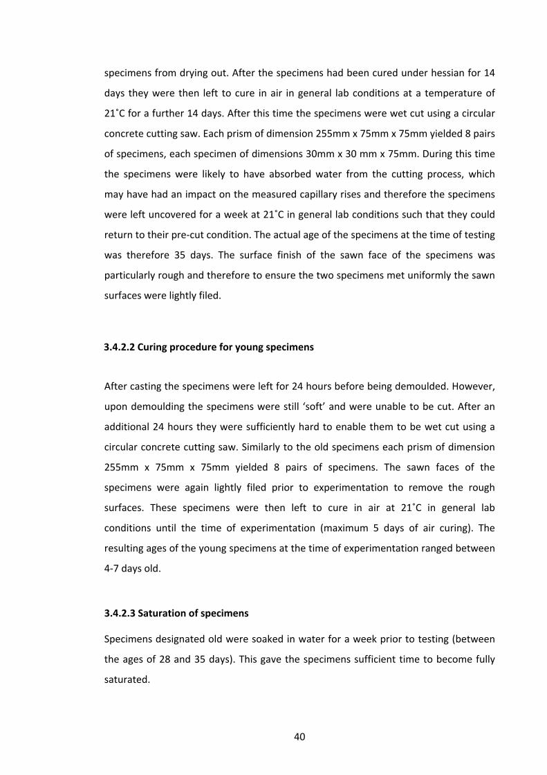
40

specimens from drying out. After the specimens had been cured under hessian for 14 

days  they were  then  left  to cure  in air  in general  lab conditions at a  temperature of 

21˚C for a further 14 days. After this time the specimens were wet cut using a circular 

concrete cutting saw. Each prism of dimension 255mm x 75mm x 75mm yielded 8 pairs 

of specimens, each specimen of dimensions 30mm x 30 mm x 75mm. During this time 

the  specimens were  likely  to  have  absorbed water  from  the  cutting  process, which 

may have had an impact on the measured capillary rises and therefore the specimens 

were left uncovered for a week at 21˚C in general lab conditions such that they could 

return to their pre‐cut condition. The actual age of the specimens at the time of testing 

was  therefore  35  days.  The  surface  finish  of  the  sawn  face  of  the  specimens was 

particularly rough and therefore to ensure the two specimens met uniformly the sawn 

surfaces were lightly filed.  

 

3.4.2.2 Curing procedure for young specimens 

 After casting the specimens were left for 24 hours before being demoulded. However, 

upon demoulding the specimens were still  ‘soft’ and were unable to be cut. After an 

additional 24 hours they were sufficiently hard to enable them to be wet cut using a 

circular concrete cutting saw. Similarly to the old specimens each prism of dimension 

255mm  x  75mm  x  75mm  yielded  8  pairs  of  specimens.  The  sawn  faces  of  the 

specimens  were  again  lightly  filed  prior  to  experimentation  to  remove  the  rough 

surfaces.  These  specimens  were  then  left  to  cure  in  air  at  21˚C  in  general  lab 

conditions  until  the  time  of  experimentation  (maximum  5  days  of  air  curing).  The 

resulting ages of the young specimens at the time of experimentation ranged between 

4‐7 days old.  

 

3.4.2.3 Saturation of specimens 

Specimens designated old were soaked  in water for a week prior to testing (between 

the ages of 28 and 35 days). This gave the specimens sufficient time to become fully 

saturated. 

41

3.5 Crack configurations and apertures 

Four crack configurations have been used  in this study and their form and method of 

manufacture  is  discussed  in  more  detail  below.  In  summary  the  four  crack 

configurations  include planar,  tapered,  tortuous and natural cracks. A  range of crack 

apertures were achieved with short lengths of steel, nickel or tin wires with diameters 

varying  from 0.094 – 1.214 mm. The diameters of  the wires were measured using a 

vernier caliper over various positions along a piece of the wire. The apertures created 

were  then measured with  a  portable  crack width microscope  and  the  actual  crack 

aperture recorded.  

 

3.5.1. Planar and tapered cracks 

The planar and tapered experiments use both old and young specimens. For the planar 

tests wires of  a  constant  diameter were  placed  between  the  two  specimens  at  the 

bottom, middle and top of the specimens, as  indicated  in figure 10a. For the tapered 

experiments wires were placed at the bottom and the top of the specimens only, with 

the wire at  the  top of  the  specimen having a  smaller diameter  than  the wire at  the 

base  of  the  specimen,  as  shown  in  figure  10b.  The  ensemble  was  then  clamped 

together to keep the wires in place. 

 

 

 

Figure 10: A Schematic representation of a) planar and b) tapered crack configuration 

 

 

Wires 

Washers 

Clamps 

Tray   Fluid 

42

3.5.2 Tortuous crack investigation 

 

Tortuous cracks were created with  the use of 2mm  folded steel plates. These plates 

were manufactured so that angle of the flow path deviated from the vertical by ± 5° 

Tortuous cracks with 2  flow path angles  (3 nodes) and 4  flow path angles  (5 nodes) 

were created, as shown  in  figure 11 a and b respectively. Prior to casting, the plates 

were  covered  in demoulding oil  to ensure  that  they would not bond  to  the mortar. 

They were  then manually held  in place during casting. The  same mixing and  casting 

procedure was used as described in section 3.4.1. 

 

(a) 

 

(b) 

 

Figure 11: Tapered crack of a) 3 nodes and b) 5 nodes achieved using folded steel plates 

 

Upon demoulding  and  removal of  the  steel plates,  the  surfaces  in  contact with  the 

mould oil were wiped  thoroughly with acetone  to ensure  that no oil was  left on  the 

surface to  influence capillary flow measurements. Wires of constant diameter, over a 

3 node folded steel plate placed vertically in the mould. 

5 node folded steel plate placed vertically in the mould. 

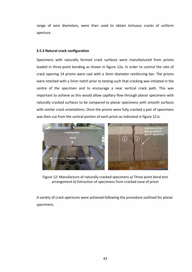
43

range  of  wire  diameters,  were  then  used  to  obtain  tortuous  cracks  of  uniform 

aperture. 

 

3.5.3 Natural crack configuration 

Specimens  with  naturally  formed  crack  surfaces  were  manufactured  from  prisms 

loaded  in three‐point bending as shown  in  figure 12a.  In order to control the rate of 

crack opening 14 prisms were cast with a 3mm diameter reinforcing bar. The prisms 

were notched with a 5mm notch prior to testing such that cracking was initiated in the 

centre  of  the  specimen  and  to  encourage  a  near  vertical  crack  path.  This  was 

important to achieve as this would allow capillary flow through planar specimens with 

naturally cracked surfaces to be compared to planar specimens with smooth surfaces 

with similar crack orientations. Once the prisms were fully cracked a pair of specimens 

was then cut from the central portion of each prism as indicated in figure 12 b.  

      

Figure 12: Manufacture of naturally cracked specimens a) Three point bend test arrangement b) Extraction of specimens from cracked zone of prism 

 

A variety of crack apertures were achieved following the procedure outlined for planar 

specimens. 

 

 

 

 

Indication of cut lines to achieve pair of specimens 

2 1

Supports 

      Notch 

       Loading point 

44

3.6 Flow agents 

3.6.1 Water and Cyanoacrylate 

 

Two  types  of  fluid  were  used  as  flow  agents  in  the  experiments,  the  physical 

parameters  of  which  are  given  in  table  3.  The  first  fluid  was  tap  water  at  room 

temperature (21°C). The second fluid was a  low viscosity, single agent, cyanoacrylate 

adhesive  (PC20  supplied by Cyanotech  Ltd.)  The data  sheet  for  the  cyanoacrylate  is 

supplied in Appendix B. The capillary flow of cyanoacrylate is particularly relevant as it 

has been successfully used by Joseph et al. (2010)  in a number of self healing studies 

performed in the same laboratory.  

 

Glass  capillary  tubes of  known diameter were used  to  calculate  the  viscosity of  the 

cyanoacrylate  in the experiments. Images of the contact angle between the meniscus 

and  the  wall  of  the  capillary  tube  were  captured  using  a  portable  crack  width 

microscope  and  digital  camera  and  together with  the  level  of  capillary  rise  height 

observed  and  the  density  of  the  cyanoacrylate,  the  viscosity  could  be  calculated. 

However,  the  viscosity  of  cyanoacrylate  changes  over  time  when  in  normal 

atmospheric  conditions.  Therefore,  measurements  of  the  change  in  viscosity  have 

been recorded. 

 

Table 3: Physical properties of flow agents used in the experimental work 

Fluid  Viscosity  

(Ns/m2) Surface Tension  

(N/m) 

Density  

(kg/m3) 

Water  0.892  0.0728  1000 

Cyanoacrylate  Varies see calculation Chapter 5 

0.0334  1060 

 

45

Silica  fume/water slurry  in a 50:50 mix by mass was considered as a  flow agent, but 

was  dismissed  during  the  early  stages  of  the  experimental  programme  due  to 

difficulties in achieving capillary flow with the silica fume in small capillaries. 

 

3.6.2 Xanthan gum 

In order to investigate the capillary flow time of a fluid with a viscosity equal to that of 

cyanoacrylate without  the  ‘curing effect’,  xanthan  gum was used. Xanthan  gum  is  a 

biological additive that can be added to fluids to increase their viscosity. Xanthan gum 

is a unique substance commonly found in food, cosmetic and industrial additives. It is a 

polysaccharide,  a  carbohydrate  and  is  usually  produced  by  fermentation  process. 

During  fermentation,  a  strain  of  bacteria  (Xanthomonas  campestris)  is  added  to 

glucose  or  sucrose  (i.e.  corn  sugar)  which  turns  them  into  a  gum.  Different 

concentrations  of  xanthan  gum  in water were  used  to  obtain  a  fluid  of  equivalent 

viscosity  (i.e.  with  the  same  rise  height)  as  that  of  cyanoacrylate.  The  amount  of 

Xanthan gum used in the experiments was calculated as 0.016g per 100ml of water.  

 

It must  be noted  that  rise  height depends  on  equation  5.1  in Chapter  5.  Therefore 

adding  the equivalent xanthan gum means  that  there  is  the  same combined  surface 

tension and contact angle term but not necessarily the same viscosity. 

 

3.7 Experimental details 

3.7.1 Data capturing technique 

High‐speed video cameras have been an excellent tool for capturing a moving process 

at  an  accelerated  rate.  High  speed  cameras  are  used  to  look  at  capturing  process 

control, process engineering and other small areas of research. Motioneer high‐speed 

video  cameras  that  have  been  selected  for  these  particular  experiments  and  can 

record up to 32,000 frames a second. This method allowed the rise height of the fluid 

through  the  crack  to  be  recorded  and  then  replayed  at  a  slower  rate  for  data 

processing purposes.  

46

In order to capture the full rise height of the fluid the experiments were recorded at 

250 frames per second. This was chosen after preliminary testing using the cameras to 

determine  an  appropriate  frame  rate  for  this  particular  experimental  arrangement. 

The previous work performed by the author presented in the literature review informs 

the reader that a shortcoming in the experimentation was that capillary flow had only 

been  recorded  at one  final height  at  a  time  at  three minutes.  The use of  the high‐

speed video  cameras enabled  the  full  flow history of  the  fluid  in  the  capillary  to be 

recorded accurate rise height with time measurements to be obtained. 

 

A scaled piece of laminated graph paper was used as the measurement tool for looking 

at the overall capillary rise height within the specimen. This method allows rise height 

to an accuracy of 0.5mm to be measured. The rise height with respect to the rise time 

was then obtained. Capillary flow was measured over a total time of 16 seconds which 

includes  the  addition  of  the  flow  agent  to  the  container where  the  specimens  are 

placed. 

 

3.7.2 Lighting 

Lighting was required in order to gain clear visibility through the simulated cracks. Two 

spot  lights were used  to  illuminate  the  front of  the specimens so  that  the  laminated 

scale could be seen on the camera, and two halogen  lights, with adjustable  intensity 

were placed directly behind the specimens to illuminate the crack. The larger the crack 

size, the less light was needed, therefore the lights behind the crack were adjusted in 

response  to  this.  Lighting  in  the  experimental work  looking  at  natural  cracks was  a 

particular challenge due to the tortuosity of the crack in two dimensions and therefore 

there was  difficulty  in  shining  the  light  provided  by  the  halogen  lamp  through  the 

entire  crack plane.  The  solution employed was  to  add  fluorescein  to  the water  and 

conduct the experiment in a darkened cabinet under an Ultra‐Violet (UV) light. The UV 

light also provided sufficient light to illuminate the laminated scale. This set up can be 

seen in figure 13.  

47

    

Figure 13: Image of natural crack experimental arrangement under UV lighting 

 

3.7.3 Experimental arrangement 

The  experimental  arrangement  is  shown  in  figure  14.  Initially,  each  specimen was 

weighed and its weight recorded. The wires were then placed onto the specimens and 

then  they were  clamped  together  (as discussed previously). The  clamped  specimens 

were then placed into a tray of dimensions 12 x 125 x 125 mm on top of two washers. 

Washers were used  to  raise  the  specimens  1.38 mm  above  the base of  the  tray  to 

ensure the  fluid would be able to  flow underneath the specimen and have access  to 

the base of the capillary.  

 

48

 

Figure 14: Experimental arrangement 

 

The  horizontal  distance  between  the  specimen  and  the  camera was  approximately 

300‐400 mm. This distance varied as a result of the  focal range of the  lens. Accurate 

measurements of rise height depended on the legibility of the scale and clarity of the 

meniscus position in the crack. For measurement of capillary flow on naturally cracked 

specimens  the  camera was placed  inside  the darkened  cabinet with  the  specimens, 

maintaining the same horizontal spacing as stated above. 

 

Once  the experiment was set up  the camera  recording sequence was  then  triggered 

and a predetermined volume of fluid, as detailed  in Table 4 was poured  immediately 

into  the  tray. The volumes  for  the cyanoacrylate  tests varied as  it was a known  fact 

that once cyanoacrylate is in contact with air, it starts to cure therefore it was difficult 

to establish exact cyanoacrylate quantities  in the experiment. However, each volume 

of flow agent used was sufficient to allow for capillary flow. 

 

Clamp

Laminated measuring  scale

Specimen Tray

Spotlight

Specimens

High Speed Video Camera 

49

Table 4: Quantities of fluid used in each experiment 

Fluid Volume of fluid used 

(ml) 

Water  50 

Cyanoacrylate  30‐50 

Xanthan gum  50 

 

Once  capillary  rise  had  occurred  recording  was  stopped  and  the  specimens  were 

immediately  taken  from  the  tray  and  each  one weighed.  This was  to  examine  the 

quantity of fluid adsorbed into the mortar matrix during the experiment to determine 

whether this had an effect on the rate and level of capillary rise observed. By weighing 

them  immediately, absorption of the  fluid over the same timescale  for all specimens 

was achieved. 

 

3.7.4 Data processing  

As there were a total of 16800 frames for each video clip, only the frames showing the 

movement of the fluid in the crack were retained. The end of capillary flow was taken 

as the point where no further rise height occurred with time. The reason for this is that 

it is the initial stages of capillary flow that are of importance, particularly in autonomic 

healing when  there  is a high potential  for  rapid hardening of  the healing agents and 

therefore, even though there will be further capillary rise over time,  it  is the first few 

seconds that are of interest. 

 

 

 

  50

Chapter 4 

Experimental Results and Discussions 

 

 

 

This  chapter  considers  the  results  from  the  experimental  work  undertaken  in  the 

laboratory. The experimental results can be considered in five distinct sections. These 

are  the  effect  of  crack  aperture;  effect  of  crack  configuration;  effect of  flow  agent; 

effect of specimen age and effect of specimen saturation on the capillary rise response 

of  liquid  flow  in  discrete  cracks  in  cementitious materials.  The  results  presented  in 

each  section  are  generally  grouped  and  discussed  in  terms  of  crack  configuration 

before further comparisons are made. 

 

The majority of the experiments were performed in triplicate and therefore, due to the 

substantial quantity of data available, only  the average  result  from  the experiments 

has  generally  been  selected  and  presented  in  this  chapter. However,  all  results  are 

given in Appendix C.  

 

Due  to  the positioning of  the  spacers,  the  field of  view of  the  camera  and  the  tray 

covering 12mm of the base of the scale, the rise heights are only available from 12mm 

upwards and the time at which 12mm was observed was taken as zero. Therefore the 

time and rise heights  indicated  in the figures do not represent the full history of fluid 

flow. Therefore, when comparing results and  looking at  the rate of capillary rise  it  is 

important  to  recognise  the  adjustment  that  has  been  made.  All  data  has  been 

extracted from the experimental videos that can be found in Appendix D. 

 

4.1 Effect of crack aperture 

 

The effect of the crack aperture on the capillary rise response of water is presented in 

this  section  and  is discussed  for  a planar  crack  configuration only. The  capillary  rise 

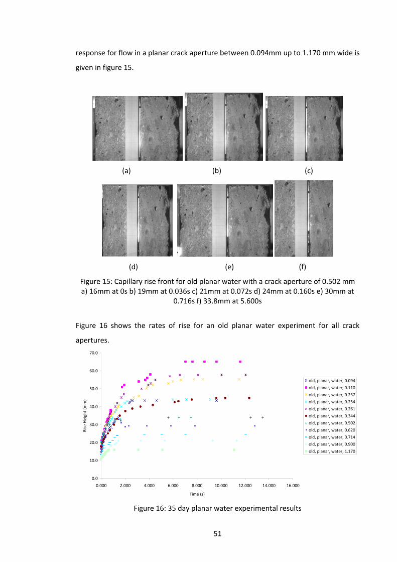
  51

response for flow in a planar crack aperture between 0.094mm up to 1.170 mm wide is 

given in figure 15.  

 

     

(a)                  (b)              (c) 

      

(d)        (e)       (f) 

Figure 15: Capillary rise front for old planar water with a crack aperture of 0.502 mm a) 16mm at 0s b) 19mm at 0.036s c) 21mm at 0.072s d) 24mm at 0.160s e) 30mm at 

0.716s f) 33.8mm at 5.600s  

Figure  16  shows  the  rates  of  rise  for  an  old  planar water  experiment  for  all  crack 

apertures. 

0.0

10.0

20.0

30.0

40.0

50.0

60.0

70.0

0.000 2.000 4.000 6.000 8.000 10.000 12.000 14.000 16.000

Time (s)

Rise Height (mm)

old, planar, water, 0.094

old, planar, water, 0.110

old, planar, water, 0.237

old, planar, water, 0.254

old, planar, water, 0.261

old, planar, water, 0.344

old, planar, water, 0.502

old, planar, water, 0.620

old, planar, water, 0.714

old, planar, water, 0.900

old, planar, water, 1.170

 Figure 16: 35 day planar water experimental results 

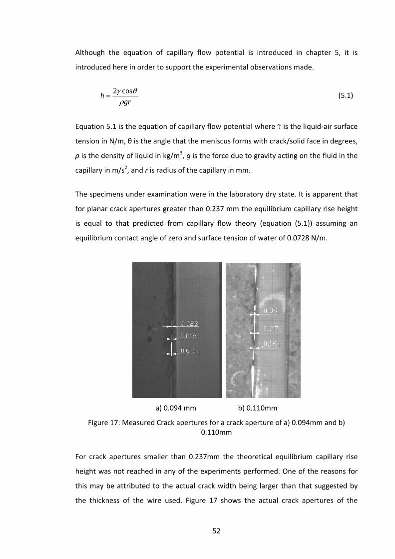
  52

Although  the  equation  of  capillary  flow  potential  is  introduced  in  chapter  5,  it  is 

introduced here in order to support the experimental observations made.  

grh

ρθγ cos2

=                   (5.1) 

Equation 5.1 is the equation of capillary flow potential where   is the liquid‐air surface 

tension in N/m, θ is the angle that the meniscus forms with crack/solid face in degrees, 

ρ is the density of liquid in kg/m3, g is the force due to gravity acting on the fluid in the 

capillary in m/s2, and r is radius of the capillary in mm.   

The specimens under examination were in the laboratory dry state. It is apparent that 

for planar crack apertures greater than 0.237 mm the equilibrium capillary rise height 

is  equal  to  that  predicted  from  capillary  flow  theory  (equation  (5.1))  assuming  an 

equilibrium contact angle of zero and surface tension of water of 0.0728 N/m.  

 

    

a) 0.094 mm          b) 0.110mm 

Figure 17: Measured Crack apertures for a crack aperture of a) 0.094mm and b) 0.110mm 

 

For  crack  apertures  smaller  than  0.237mm  the  theoretical  equilibrium  capillary  rise 

height was not reached  in any of the experiments performed. One of the reasons for 

this may be attributed  to  the actual crack width being  larger  than  that suggested by 

the  thickness  of  the wire  used.  Figure  17  shows  the  actual  crack  apertures  of  the 

  53

experiment  determined  from  a  video  image.  It  is  shown  in  figure  17  that  for  an 

assumed crack aperture of 0.094 measurements of actual crack apertures range from 

0.016mm to 0.023mm. This is due to variations of the mortar faces caused through the 

manufacture of the specimens and achieving a uniform clamping force over the height 

of  the specimen. Although,  this effect will be apparent  in  the majority of  the  tests  it 

has a greater effect on the capillary rise heights in the narrower capillaries. This is why 

the  final  rise height  is  a  lot  lower  than  the expected  rise height. Using  the  average 

value of rise height from the experiment and the equation of flow 5.1 the comparisons 

of  rise height versus  crack aperture  can be made. These are presented  towards  the 

end of this section. 

 

Another reason for the changes  in final rise height differences could be attributed to 

the changes of the specimen weight due to absorption of fluid during the experiment. 

These values are given in Table 5. The table also gives an indication of the magnitude 

of variation observed in the experimental results.  

 

Table 5: Changes in weight of 35 day planar water experiments 

Crack aperture 

(mm) 

Weight increase of specimens

(g) 

Equilibrium rise heights  

(mm) 

  Test #1  Test #2  Test #3 Test #1  Test #2  Test #3 

0.094  2.0  1.5  2.5  35.0  43.5  40.5 

0.237  2.5  3.0  3.5  30.0  55.1  65.0 

0.261  2.0  2.5  2.5  16.0  57.8  57.8 

0.620  1.5  1.5  2.0  24.0  29.2  30.5 

1.170  1.0  1.0  2.0  20.9  15.9  14.5 

 

As seen in the table above, the experiments with a lower equilibrium rise height have 

greater  increases  in weight  indicating greater absorption of water  into  the matrix of 

the mortar  specimen.  As  absorption  occurs  through  the  open  pores  in  the  cement 

matrix, fluid stays in the voids therefore increasing the overall weight of the specimen. 

It can be concluded  that  flow away  from  the main capillary channel  into  the cement 

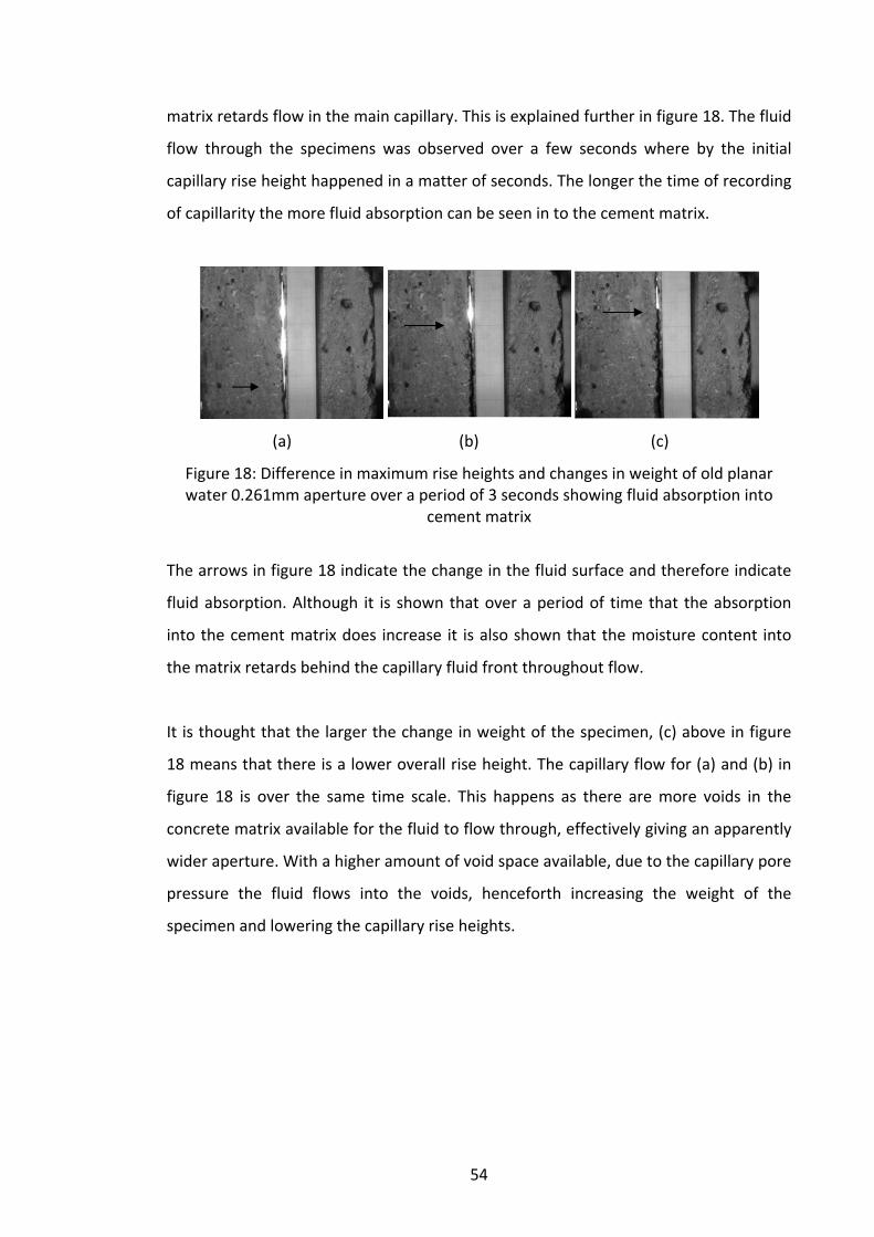
  54

matrix retards flow in the main capillary. This is explained further in figure 18. The fluid 

flow  through  the  specimens was  observed  over  a  few  seconds where  by  the  initial 

capillary rise height happened in a matter of seconds. The longer the time of recording 

of capillarity the more fluid absorption can be seen in to the cement matrix. 

 

     

      (a)              (b)         (c) 

Figure 18: Difference in maximum rise heights and changes in weight of old planar water 0.261mm aperture over a period of 3 seconds showing fluid absorption into 

cement matrix  

The arrows in figure 18 indicate the change in the fluid surface and therefore indicate 

fluid absorption. Although  it  is shown  that over a period of  time  that the absorption 

into the cement matrix does  increase  it  is also shown that the moisture content  into 

the matrix retards behind the capillary fluid front throughout flow. 

 

It  is thought that the  larger the change  in weight of the specimen, (c) above  in figure 

18 means that there  is a  lower overall rise height. The capillary flow for (a) and (b) in 

figure 18  is over  the  same  time  scale.  This happens  as  there  are more  voids  in  the 

concrete matrix available for the fluid to flow through, effectively giving an apparently 

wider aperture. With a higher amount of void space available, due to the capillary pore 

pressure  the  fluid  flows  into  the  voids,  henceforth  increasing  the  weight  of  the 

specimen and lowering the capillary rise heights.  

 

  55

0

20

40

60

80

100

120

140

160

180

0 0.2 0.4 0.6 0.8 1 1.2 1.4

Final Rise Height (mm)

Crack Aperture (mm)

Old planar data

Theoretical Data

 

Figure 19: Comparison of planar crack aperture with final rise heights for 35 day old specimens 

 

Previously,  average  results  for  each  specimen have been presented  to demonstrate 

the  effect of  crack width on  the  capillary  rise  response  and  the  final  rise height.  In 

order  to examine  the variation between  the  tests performed at each crack aperture, 

the final rise height has been extracted for each experiment and is shown in figure 19 

for each crack aperture.  

 

At  crack  apertures  greater  than  0.344mm  the  variation  in  results  for  each  crack 

aperture  are  reasonably  consistent  and  show  a  lower  overall  spread  than  for  crack 

apertures  less  than 0.344mm. This observation helps  support  the previous  selection 

and  discussion  of  the  capillary  rise  response  and  final  rise  heights  using  only  the 

average data points 

 

The  results  presented  in  figure  19  confirm  previous  observations  that  the  final  rise 

height  associated with  the  two  smallest  apertures  are  significantly  lower  than  the 

theoretical final rise heights, calculated using equation 5.1. It  is believed that this can 

be attributed to (i) the limiting effect of the specimen height (75mm); (ii) the difficulty 

in achieving small (less than 0.110mm) crack apertures with the methods used and (iii) 

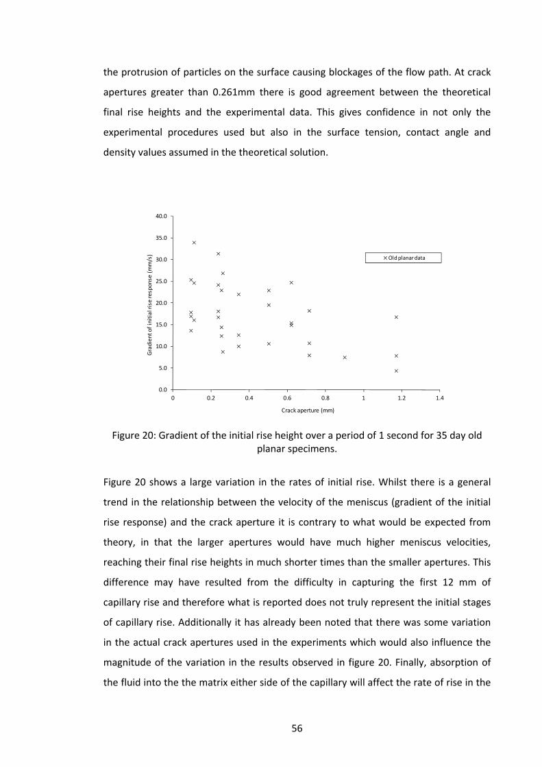
  56

the protrusion of particles on the surface causing blockages of the flow path. At crack 

apertures  greater  than  0.261mm  there  is  good  agreement  between  the  theoretical 

final  rise  heights  and  the  experimental  data.  This  gives  confidence  in  not  only  the 

experimental  procedures  used  but  also  in  the  surface  tension,  contact  angle  and 

density values assumed in the theoretical solution. 

 

0.0

5.0

10.0

15.0

20.0

25.0

30.0

35.0

40.0

0 0.2 0.4 0.6 0.8 1 1.2 1.4

Gradient of initia

l rise response (m

m/s)

Crack aperture (mm)

Old planar data

 

Figure 20: Gradient of the initial rise height over a period of 1 second for 35 day old planar specimens. 

 

Figure 20 shows a  large variation  in  the rates of  initial rise. Whilst  there  is a general 

trend  in the relationship between the velocity of the meniscus (gradient of the  initial 

rise response) and  the crack aperture  it  is contrary  to what would be expected  from 

theory,  in  that  the  larger  apertures  would  have  much  higher  meniscus  velocities, 

reaching their final rise heights in much shorter times than the smaller apertures. This 

difference  may  have  resulted  from  the  difficulty  in  capturing  the  first  12  mm  of 

capillary rise and therefore what is reported does not truly represent the initial stages 

of capillary rise. Additionally  it has already been noted that there was some variation 

in the actual crack apertures used  in the experiments which would also  influence the 

magnitude of the variation  in the results observed  in  figure 20. Finally, absorption of 

the fluid into the the matrix either side of the capillary will affect the rate of rise in the 

  57

main  capillary  channel,  although without  further measurement  and  interrogation of 

the video data this is difficult to quantify.  

 

4.2 Effect of crack configuration 

 

Five different crack configurations were examined as part of the experimental work in 

this  thesis,  these  were  planar;  tapered;  two  types  of  tortuous  cracks  and  natural 

cracks. This section looks at how a change in crack configuration affects capillary flow 

through cementitious materials.  

 

The  planar  results  have  already  been  considered  and  analysed.  Therefore,  the  next 

areas  of  investigation  are  tapered,  tortuous  3  and  5  nodes  and  natural  crack 

configurations.  

 

Capillary  flow  has  been  examined  for  35  day  old  tapered  crack  configurations.  This 

type of  crack  configuration has been  looked at experimentally and  the observations 

have been recorded and discussed in detail below.  

 

0.0

10.0

20.0

30.0

40.0

50.0

60.0

70.0

80.0

0.000 2.000 4.000 6.000 8.000 10.000 12.000 14.000

Time (s)

Rise Height (mm)

old, tapered, water, 0.094‐0.110

old, tapered, water, 0.110‐0.261

old, tapered, water, 0.237‐0.344

old, tapered, water, 0.344‐0.502

old, tapered, water, 0.502‐0.714

old, tapered, water, 0.714‐0.900

old, tapered, water, 0.900‐1.170

 Figure 21: 35 day tapered water experimental graphs and results 

 

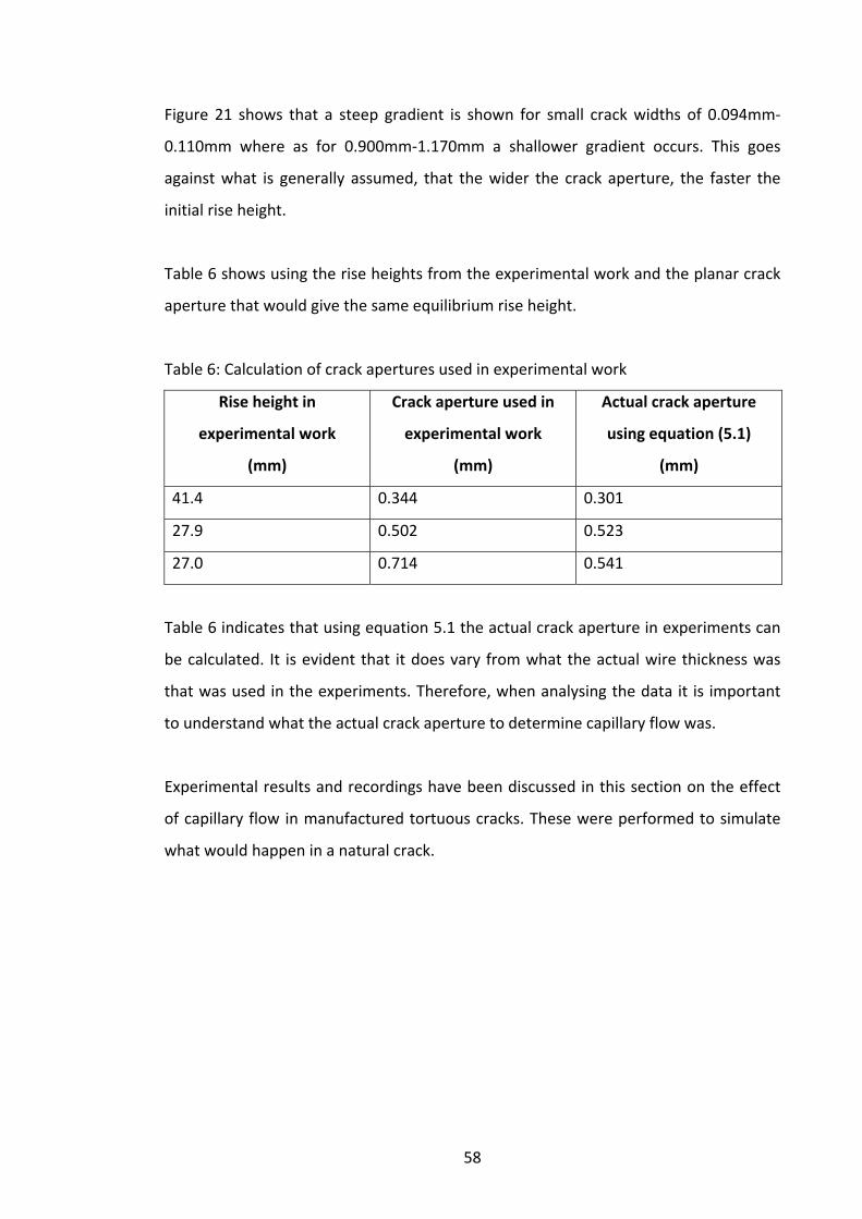
  58

Figure 21  shows  that a  steep gradient  is  shown  for  small  crack widths of 0.094mm‐

0.110mm  where  as  for  0.900mm‐1.170mm  a  shallower  gradient  occurs.  This  goes 

against what  is generally assumed,  that  the wider  the crack aperture,  the  faster  the 

initial rise height.  

 

Table 6 shows using the rise heights from the experimental work and the planar crack 

aperture that would give the same equilibrium rise height.  

 

Table 6: Calculation of crack apertures used in experimental work 

Rise height in 

experimental work  

(mm) 

Crack aperture used in 

experimental work  

(mm) 

Actual crack aperture 

using equation (5.1)  

(mm) 

41.4  0.344  0.301 

27.9  0.502  0.523 

27.0  0.714  0.541 

 

Table 6 indicates that using equation 5.1 the actual crack aperture in experiments can 

be calculated.  It  is evident that  it does vary  from what the actual wire thickness was 

that was used  in the experiments. Therefore, when analysing the data  it  is  important 

to understand what the actual crack aperture to determine capillary flow was. 

 

Experimental results and recordings have been discussed  in this section on the effect 

of capillary flow  in manufactured tortuous cracks. These were performed to simulate 

what would happen in a natural crack. 

 

  59

0.0

10.0

20.0

30.0

40.0

50.0

60.0

70.0

0.000 1.000 2.000 3.000 4.000 5.000 6.000 7.000 8.000

Time (s)

Rise Height (mm)

old, tortuous, 3 nodes, water, 0.170

old, tortuous, 3 nodes, water, 0.344

old, tortuous, 3 nodes, water, 0.502

old, tortuous, 3 nodes, water, 0.714

old, tortuous, 5 nodes, water, 0.170

old, tortuous, 5 nodes, water, 0.344

old, tortuous, 5 nodes, water, 0.502

old, tortuous, 5 nodes, water, 0.714

  

Figure 22: Effect of crack configuration, 35 day tortuous 3 nodes water and 35 day tortuous 5 nodes water 

 

Figure 22 compares 3 & 5 nodes, old tortuous water experiments with different crack 

apertures. Looking at 3 & 5 nodes with a crack aperture of 0.170 mm, there is a slight 

difference in overall rise height. The overall rise height is affected due to the change in 

the nodal number, it can be seen that there is a lower rise height for a larger number 

of nodes. However, for the  larger crack apertures the fluid does not get past the first 

nodal point. Therefore, for further experimentation spoken about in chapter six and an 

idea would be to increase the number of nodes to see what the effect of the change in 

angle would have on fluid flow. Also,  it  is clearly shown  in the graph, that the higher 

the tortuosity of the specimens, the longer time it takes to reach maximum rise height. 

The  fluid has  further  to  travel  to  get  to  an  absolute  rise height  in  a  tortuous  crack. 

Change  in  inclination  of  the  crack  reduces  the  overall  time  for  the  fluid  to  reach 

equilibrium rise height. This is shown in the theory chapter 5.  

 

Natural  cracked  specimens  have  been  used  to  determine  the  rate  of  flow  of  fluids 

through  cementitious materials  representative  of  those  found  in  current  structures. 

The experimental results have been recorded below and discussed.  

 

  60

0

20

40

60

80

100

120

140

160

180

0 0.2 0.4 0.6 0.8 1 1.2 1.4

Final Rise Height (mm)

Crack Aperture (mm)

Old tortuous 3 nodes

Old tortuous 5 nodes

Theoretical Data

 

Figure 23: Comparison of tortuous crack aperture with final rise heights for 35 day old specimens 

 

Similar  to  the  planar  crack  aperture  data  shown  previously  in  figure  19  at  tortuous 

crack  apertures  greater  than  0.344mm  the  final  rise  height  results  for  each  crack 

aperture  are  reasonably  consistent  with  those  calculated  from  theory,  with  the 

variation in the results decreasing with increasing crack aperture. 

 

The  results  presented  in  figure  23  confirm  previous  observations  that  the  final  rise 

height  associated with  the  two  smallest  apertures  are  significantly  lower  than  the 

theoretical  final  rise  heights,  again  confirming  the  difficulty  in  achieving  small  (less 

than 0.110mm)  crack  apertures with  the methods used. Moreover,  figure 23  shows 

that there  is  little difference  in the results between the 3 and the 5 node specimens, 

confirming the theory that regardless of crack inclination the fluid will always reach the 

same absolute rise height for the same crack aperture.  

 

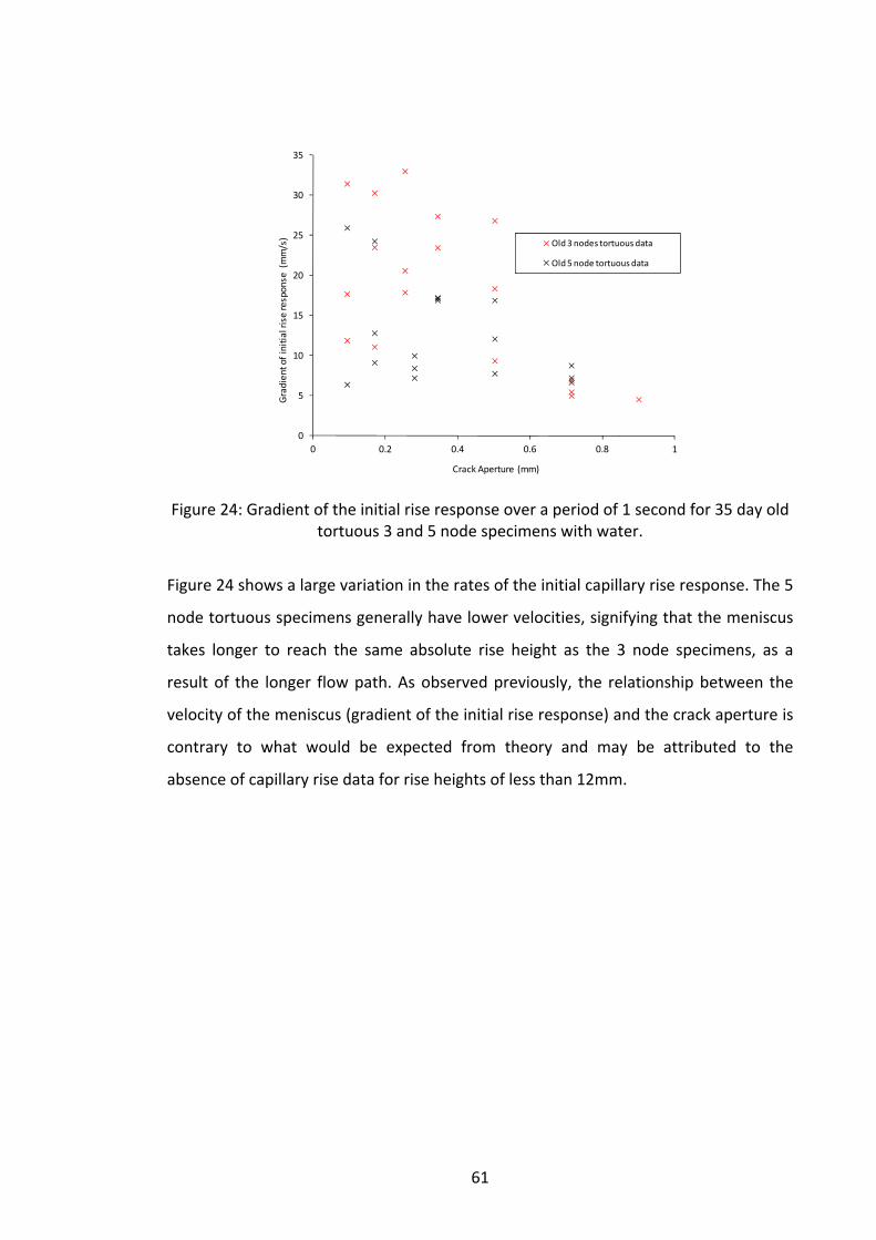
  61

0

5

10

15

20

25

30

35

0 0.2 0.4 0.6 0.8 1

Gradient of initia

l rise response  (mm/s)

Crack Aperture (mm)

Old 3 nodes tortuous data

Old 5 node tortuous data

 

Figure 24: Gradient of the initial rise response over a period of 1 second for 35 day old tortuous 3 and 5 node specimens with water. 

 

Figure 24 shows a large variation in the rates of the initial capillary rise response. The 5 

node tortuous specimens generally have lower velocities, signifying that the meniscus 

takes  longer  to  reach  the  same  absolute  rise height  as  the  3  node  specimens,  as  a 

result of  the  longer  flow path. As observed previously,  the  relationship between  the 

velocity of the meniscus (gradient of the initial rise response) and the crack aperture is 

contrary  to  what  would  be  expected  from  theory  and  may  be  attributed  to  the 

absence of capillary rise data for rise heights of less than 12mm. 

 

  62

0.0

5.0

10.0

15.0

20.0

25.0

30.0

0.000 2.000 4.000 6.000 8.000 10.000 12.000

Time (s)

Rise Height (mm) old, natural, water, 0.170

old, natural, water, 0.280

old, natural, water, 0.344

old, natural, water, 0.502

old, natural, water, 0.620

old, natural, water, 0.714

 Figure 25: 35 day natural water experimental graph and results 

 

The natural water experiments, shown in figure 25, show consistency with the theory 

of  the  capillary  flow  potential  equation  5.1  that  the  greater  the  crack width  of  the 

capillary the lower the overall rise height. Table 7 indicates for specific crack apertures 

what the corresponding rise height should be and what the experimental rise heights 

were found to be.  

 

The contact angles were measured using  images from the capillary rise height videos 

for  specific  crack  apertures.  The  angles  were  only  measured  for  planar  crack 

experiments not for tapered, tortuous or natural cracked specimens. 

 

The  contact  was  measured  using  images  of  where  the  light  shines  through  the 

specimen. 

 

 

 

 

 

 

 

 

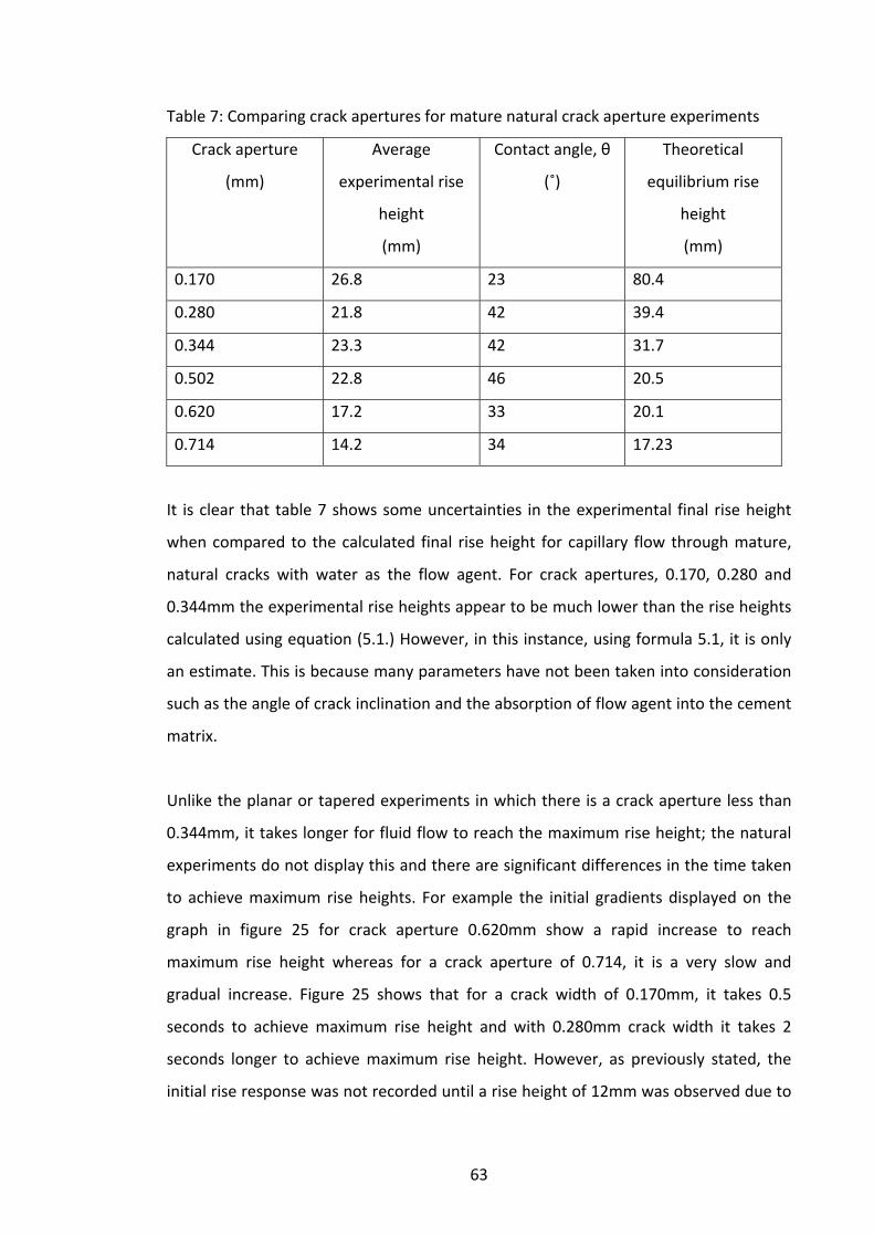
  63

Table 7: Comparing crack apertures for mature natural crack aperture experiments 

Crack aperture 

(mm) 

Average 

experimental rise 

height  

(mm) 

Contact angle, θ 

(˚) 

Theoretical 

equilibrium rise 

height  

(mm) 

0.170  26.8  23  80.4 

0.280  21.8  42  39.4 

0.344  23.3  42  31.7 

0.502  22.8  46  20.5 

0.620  17.2  33  20.1 

0.714  14.2  34  17.23 

 

It  is clear that table 7 shows some uncertainties  in the experimental  final rise height 

when compared  to  the calculated  final  rise height  for capillary  flow  through mature, 

natural  cracks with water  as  the  flow  agent.  For  crack  apertures,  0.170,  0.280  and 

0.344mm the experimental rise heights appear to be much lower than the rise heights 

calculated using equation (5.1.) However, in this instance, using formula 5.1, it is only 

an estimate. This is because many parameters have not been taken into consideration 

such as the angle of crack inclination and the absorption of flow agent into the cement 

matrix.  

 

Unlike the planar or tapered experiments  in which there  is a crack aperture  less than 

0.344mm, it takes longer for fluid flow to reach the maximum rise height; the natural 

experiments do not display this and there are significant differences in the time taken 

to achieve maximum  rise heights. For example  the  initial gradients displayed on  the 

graph  in  figure  25  for  crack  aperture  0.620mm  show  a  rapid  increase  to  reach 

maximum  rise  height whereas  for  a  crack  aperture  of  0.714,  it  is  a  very  slow  and 

gradual  increase.  Figure  25  shows  that  for  a  crack width  of  0.170mm,  it  takes  0.5 

seconds  to  achieve maximum  rise  height  and with  0.280mm  crack width  it  takes  2 

seconds  longer  to  achieve maximum  rise height. However,  as previously  stated,  the 

initial rise response was not recorded until a rise height of 12mm was observed due to 

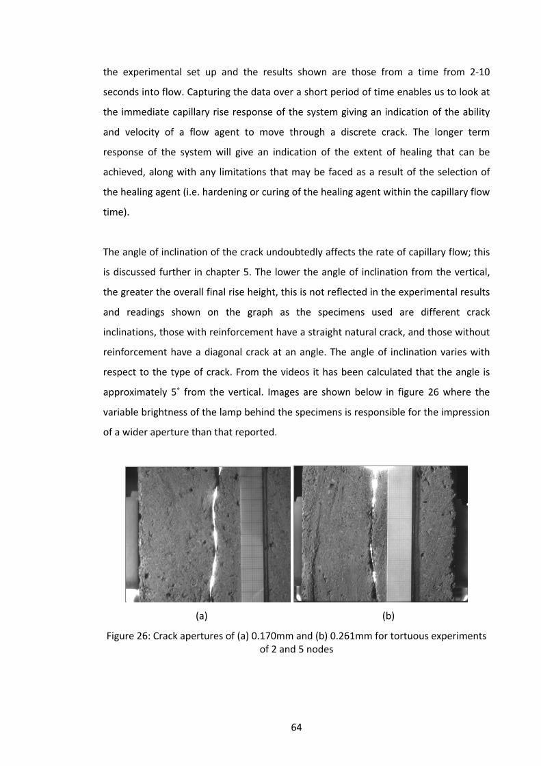
  64

the  experimental  set  up  and  the  results  shown  are  those  from  a  time  from  2‐10 

seconds into flow. Capturing the data over a short period of time enables us to look at 

the  immediate capillary rise response of the system giving an  indication of the ability 

and  velocity  of  a  flow  agent  to  move  through  a  discrete  crack.  The  longer  term 

response  of  the  system will  give  an  indication  of  the  extent  of  healing  that  can  be 

achieved, along with any  limitations that may be faced as a result of the selection of 

the healing agent (i.e. hardening or curing of the healing agent within the capillary flow 

time).  

 

The angle of inclination of the crack undoubtedly affects the rate of capillary flow; this 

is discussed further  in chapter 5. The  lower the angle of  inclination from the vertical, 

the greater the overall final rise height, this is not reflected in the experimental results 

and  readings  shown  on  the  graph  as  the  specimens  used  are  different  crack 

inclinations, those with reinforcement have a straight natural crack, and those without 

reinforcement have a diagonal crack at an angle. The angle of  inclination varies with 

respect to the type of crack. From the videos  it has been calculated that the angle  is 

approximately 5˚  from  the vertical.  Images are  shown below  in  figure 26 where  the 

variable brightness of the lamp behind the specimens is responsible for the impression 

of a wider aperture than that reported.  

 

   

               (a)                 (b) 

Figure 26: Crack apertures of (a) 0.170mm and (b) 0.261mm for tortuous experiments of 2 and 5 nodes 

 

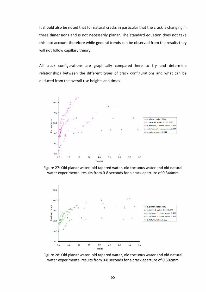
  65

It should also be noted that for natural cracks in particular that the crack is changing in 

three dimensions and  is not necessarily planar. The standard equation does not take 

this into account therefore while general trends can be observed from the results they 

will not follow capillary theory. 

 

All  crack  configurations  are  graphically  compared  here  to  try  and  determine 

relationships  between  the  different  types  of  crack  configurations  and what  can  be 

deduced from the overall rise heights and times.  

 

 

Figure 27: Old planar water, old tapered water, old tortuous water and old natural water experimental results from 0‐8 seconds for a crack aperture of 0.344mm 

 

 

Figure 28: Old planar water, old tapered water, old tortuous water and old natural water experimental results from 0‐8 seconds for a crack aperture of 0.502mm 

  66

 

 

Figure 29: Old planar water, old tapered water, old tortuous water and old natural water experimental results from 0‐8 seconds for a crack aperture of 0.714mm 

 

Looking at  figures 27  ‐ 29 shows  that at a crack width of 0.344mm,  the experiments 

display a similar maximum overall rise height  for all crack configurations. The overall 

rise heights for a crack width of 0.714 are in the similar region and only have an overall 

maximum difference  in  rise height of 10mm. Therefore,  it  is width  rather  than crack 

configuration  that  has  importance  for  achieving maximum  rise  height.  The  smallest 

overall rise height obtained was taken from the natural crack experiments. 

 

4.3 Effect of flow agent 

 

This section of the results chapter looks at the difference in overall rise heights, crack 

apertures and flow rates between water, cyanoacrylate and xanthan gum.  

 

This results section is introduced to look at the changes between the flow agents used 

in  the  experiments.  This  is  because  each  flow  agent  has  a  different  viscosity  and 

surface  tension  and  therefore  capillary  rise  heights  are  expected  to  be  different. 

Furthermore, the effect of setting times can be investigated. 

 

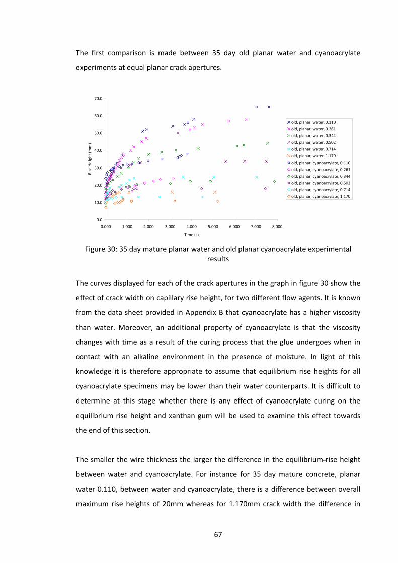
  67

The  first  comparison  is made  between  35  day  old  planar water  and  cyanoacrylate 

experiments at equal planar crack apertures. 

 

0.0

10.0

20.0

30.0

40.0

50.0

60.0

70.0

0.000 1.000 2.000 3.000 4.000 5.000 6.000 7.000 8.000

Time (s)

Rise Height (mm)

old, planar, water, 0.110

old, planar, water, 0.261

old, planar, water, 0.344

old, planar, water, 0.502

old, planar, water, 0.714

old, planar, water, 1.170

old, planar, cyanoacrylate, 0.110

old, planar, cyanoacrylate, 0.261 

old, planar, cyanoacrylate, 0.344

old, planar, cyanoacrylate, 0.502

old, planar, cyanoacrylate, 0.714

old, planar, cyanoacrylate, 1.170

 Figure 30: 35 day mature planar water and old planar cyanoacrylate experimental 

results  

The curves displayed for each of the crack apertures in the graph in figure 30 show the 

effect of crack width on capillary rise height, for two different flow agents. It is known 

from the data sheet provided  in Appendix B that cyanoacrylate has a higher viscosity 

than water. Moreover,  an  additional  property  of  cyanoacrylate  is  that  the  viscosity 

changes with time as a result of the curing process that the glue undergoes when  in 

contact  with  an  alkaline  environment  in  the  presence  of moisture.  In  light  of  this 

knowledge  it  is  therefore appropriate  to assume  that equilibrium  rise heights  for all 

cyanoacrylate specimens may be  lower than their water counterparts. It  is difficult to 

determine  at  this  stage whether  there  is  any  effect  of  cyanoacrylate  curing  on  the 

equilibrium rise height and xanthan gum will be used to examine this effect towards 

the end of this section. 

 

The smaller the wire thickness the  larger the difference  in the equilibrium rise height 

between water  and  cyanoacrylate.  For  instance  for  35  day mature  concrete,  planar 

water 0.110, between water and cyanoacrylate, there  is a difference between overall 

maximum  rise heights of 20mm whereas  for 1.170mm  crack width  the difference  in 

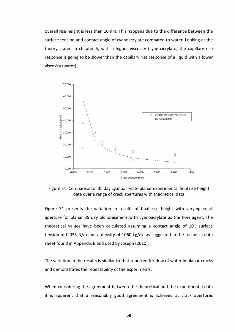
  68

overall rise height is less than 10mm. This happens due to the difference between the 

surface tension and contact angle of cyanoacrylate compared to water. Looking at the 

theory  stated  in  chapter  5, with  a  higher  viscosity  (cyanoacrylate)  the  capillary  rise 

response is going to be slower than the capillary rise response of a liquid with a lower 

viscosity (water).  

 

0.000

10.000

20.000

30.000

40.000

50.000

60.000

70.000

0.000 0.200 0.400 0.600 0.800 1.000 1.200 1.400

Final rise height (m

m)

Crack aperture (mm)

Old planar data cyanoacrylate

Theoretical Data

 

Figure 31: Comparison of 35 day cyanoacrylate planar experimental final rise height data over a range of crack apertures with theoretical data 

 

Figure  31  presents  the  variation  in  results  of  final  rise  height  with  varying  crack 

aperture  for planar 35 day old  specimens with cyanoacrylate as  the  flow agent. The 

theoretical  values  have  been  calculated  assuming  a  contact  angle  of  10˚,  surface 

tension of 0.033 N/m and a density of 1060 kg/m3 as suggested  in the technical data 

sheet found in Appendix B and used by Joseph (2010). 

 

The variation in the results is similar to that reported for flow of water in planar cracks 

and demonstrates the repeatability of the experiments.  

 

When considering the agreement between the theoretical and the experimental data 

it  is  apparent  that  a  reasonably  good  agreement  is  achieved  at  crack  apertures 

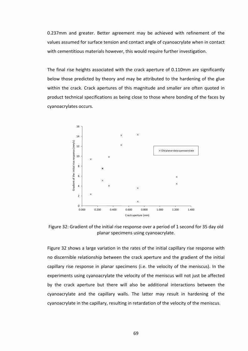
  69

0.237mm  and  greater.  Better  agreement may  be  achieved with  refinement  of  the 

values assumed for surface tension and contact angle of cyanoacrylate when in contact 

with cementitious materials however, this would require further investigation. 

 

The final rise heights associated with the crack aperture of 0.110mm are significantly 

below those predicted by theory and may be attributed to the hardening of the glue 

within  the crack. Crack apertures of  this magnitude and  smaller are often quoted  in 

product technical specifications as being close to those where bonding of the faces by 

cyanoacrylates occurs.  

0

2

4

6

8

10

12

14

16

0.000 0.200 0.400 0.600 0.800 1.000 1.200 1.400

Gradient of the

 initial rise response (m

m/s)

Crack aperture (mm)

Old planar data cyanoacrylate

 

Figure 32: Gradient of the initial rise response over a period of 1 second for 35 day old planar specimens using cyanoacrylate. 

 

Figure 32 shows a large variation in the rates of the initial capillary rise response with 

no discernible relationship between the crack aperture and the gradient of the  initial 

capillary  rise  response  in planar  specimens  (i.e.  the velocity of  the meniscus).  In  the 

experiments using cyanoacrylate the velocity of the meniscus will not just be affected 

by  the  crack  aperture  but  there  will  also  be  additional  interactions  between  the 

cyanoacrylate  and  the  capillary  walls.  The  latter  may  result  in  hardening  of  the 

cyanoacrylate in the capillary, resulting in retardation of the velocity of the meniscus. 

 

  70

0.0

10.0

20.0

30.0

40.0

50.0

60.0

70.0

0.000 0.200 0.400 0.600 0.800 1.000

Final Rise Height (mm)

Crack aperture (mm)

Old 3 node tortuous data cyanoacrylate

Old 5 node tortuous data cyanoacrylate

Theoretical data

 

Figure 33: Comparison of 35 day cyanoacrylate tortuous experimental final rise height data over a range of crack apertures with theoretical data 

 

As can be seen in figure 33 the cyanoacrylate experimental data for the 3 and 5 node 

tortuous specimens agrees reasonably well with the theory. Unlike the data presented 

in figure 31 the majority of the tortuous data falls slightly below the theoretical values. 

As has been  repeatedly noted  throughout Section 4  this may be due  to variations  in 

the  actual  crack  apertures  used  in  the  experiments.  Furthermore,  there  may  be 

evidence of  cyanoacrylate healing  in  the  two  smallest  crack  apertures,  in which  the 

theoretical rise heights were not achieved. This is further supported by the difficulty in 

physically pulling these specimens apart  immediately after the capillary rise response 

had been captured.  

 

For all crack apertures the rise heights associated with the 5 node tortuous specimens 

are generally  lower  than  their 3 node counterparts. This may  reflect  the  longer  flow 

path  of  the  cyanoacrylate  in  the  5  node  tortuous  specimens  resulting  in  additional 

curing and hardening occurring, prohibiting the full rise height from being achieved.  

 

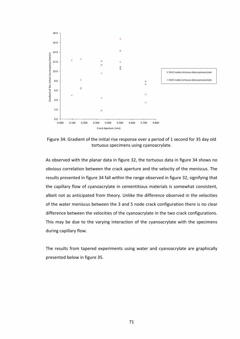
  71

0.0

2.0

4.0

6.0

8.0

10.0

12.0

14.0

16.0

18.0

0.000 0.100 0.200 0.300 0.400 0.500 0.600 0.700 0.800

Gradient of the

 initial rise response (m

m/s)

Crack Aperture (mm)

Old 3 nodes tortuous data cyanoacrylate

Old 5 nodes tortuous data cyanoacrylate

 

Figure 34: Gradient of the initial rise response over a period of 1 second for 35 day old tortuous specimens using cyanoacrylate. 

 

As observed with the planar data in figure 32, the tortuous data in figure 34 shows no 

obvious correlation between the crack aperture and the velocity of the meniscus. The 

results presented in figure 34 fall within the range observed in figure 32, signifying that 

the capillary  flow of cyanoacrylate  in cementitious materials  is somewhat consistent, 

albeit not as anticipated from theory. Unlike the difference observed  in the velocities 

of the water meniscus between the 3 and 5 node crack configuration there is no clear 

difference between the velocities of the cyanoacrylate in the two crack configurations. 

This may be due  to  the varying  interaction of  the cyanoacrylate with  the  specimens 

during capillary flow. 

 

The  results  from  tapered experiments using water and cyanoacrylate are graphically 

presented below in figure 35. 

 

  72

0.0

10.0

20.0

30.0

40.0

50.0

60.0

70.0

0.000 1.000 2.000 3.000 4.000 5.000 6.000 7.000 8.000

Time (s)

Rise Height (mm) old, tapered, water, 0.094‐0.110

old, tapered, water, 0.344‐0.502

old, tapered, water, 0.502‐0.714

old, tapered, cyanoacrylate, 0.094‐0.110

old, tapered, cyanoacrylate, 0.344‐0.502

old, tapered, cyanoacylate, 0.502‐0.714

  Figure 35: 35 day mature specimens tapered water and 35 day mature specimens 

tapered cyanoacrylate experimental results  

All 35 day mature tapered water and cyanoacrylate data again  follow theory, that  is, 

the smaller the crack aperture the larger the overall rise height.  

 

It  can  be  seen  looking  at  the  gradients  of  both  the  water  and  the  cyanoacrylate 

experiments  that  the  water  experiments  initial  gradients  are  steeper.  However, 

previously stated, what  is shown  is not  the  initial rise height, only  the response past 

12mm rise height. Looking at equation 5.1 and theory in chapter 5 these observations 

do again follow theory as cyanoacrylate has a lower viscosity than water, however it is 

not  certain  that  it  can  be  assumed  that  this  prevents  it  reaching  its maximum  rise 

height in a fast amount of time. This may also occur due to the cyanoacrylate setting.  

 

Table  8:  Comparison  of  cyanoacrylate  theoretical  rise  height with  experimental  rise height 

Crack aperture 

(mm) 

Theoretical rise height 

(mm) 

Experimental average rise 

height  

(mm) 

0.261  24.3  23.1 

0.344  18.4  22.3 

0.502  12.6  18.0 

 

  73

Table  8  shows  that  the  theoretical  rise  height  of  cyanoacrylate  in  a  specific  crack 

aperture  appears  to  be  similar  to  the  average  experimental  rise  height  recorded. 

However,  from  the  experimental  tests  it  can  be  seen  that  the  values  for  the 

experimental average rise height is higher as the crack apertures could be smaller. This 

is due to the wires losing shape in the process of being clamped. 

 

When considering the effect that a change  in  inclination of cracks has on the rates of 

fluid flow through capillaries, as performed in the tortuous experiments it can be seen 

that  for  35  day  mature  specimens  tortuous  3  nodes  water  the  crack  aperture  of 

0.170mm  has  an  unexpected  capillary  rise  response.  Between  1  and  2  seconds  the 

overall rate of flow slows down in comparison to the rest of the experiment. The areas 

where  there  is  a  gentle  gradient,  is where  there  is  absorption  of  the  fluid  into  the 

cement matrix,  and  areas where  there  is  a  steep  gradient  is where  the  fluid  rises 

rapidly due to the capillary pore pressure. This statement  is confirmed by the videos 

found in the attached data to this thesis but it is also shown in figure 36.  

 

The retardation of the fluid shown below  in the graph (figure 36) for old, tortuous, 3 

nodes, water, 0.170mm, is as a result of the wire restricting the flow of the fluid in the 

channel.  The wire  in  this  instance  acted  as  a  blockage  in  the  flow  path.  In  further 

experiments  the  spacer wires were  placed  outside  of  the  anticipated  flow  areas  to 

reduce the occurrence of this.  

 

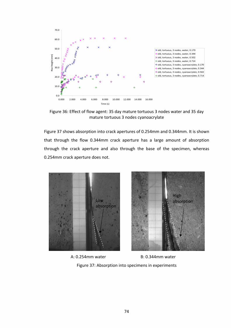
  74

0.0

10.0

20.0

30.0

40.0

50.0

60.0

70.0

0.000 2.000 4.000 6.000 8.000 10.000 12.000 14.000 16.000

Time (s)

Rise Height (mm)

old, tortuous, 3 nodes, water, 0.170

old, tortuous, 3 nodes, water, 0.344

old, tortuous, 3 nodes, water, 0.502

old, tortuous, 3 nodes, water, 0.714

old, tortuous, 3 nodes, cyanoacrylate, 0.170

old, tortuous, 3 nodes, cyanoacrylate, 0.344

old, tortuous, 3 nodes, cyanoacrylate, 0.502

old, tortuous, 3 nodes, cyanoacrylate, 0.714

  Figure 36: Effect of flow agent: 35 day mature tortuous 3 nodes water and 35 day 

mature tortuous 3 nodes cyanoacrylate  

Figure 37 shows absorption into crack apertures of 0.254mm and 0.344mm. It is shown 

that  through  the  flow  0.344mm  crack  aperture  has  a  large  amount  of  absorption 

through  the  crack  aperture  and  also  through  the  base  of  the  specimen,  whereas 

0.254mm crack aperture does not.  

 

             

A: 0.254mm water      B: 0.344mm water   

Figure 37: Absorption into specimens in experiments 

 

 

 

Low absorption 

High absorption 

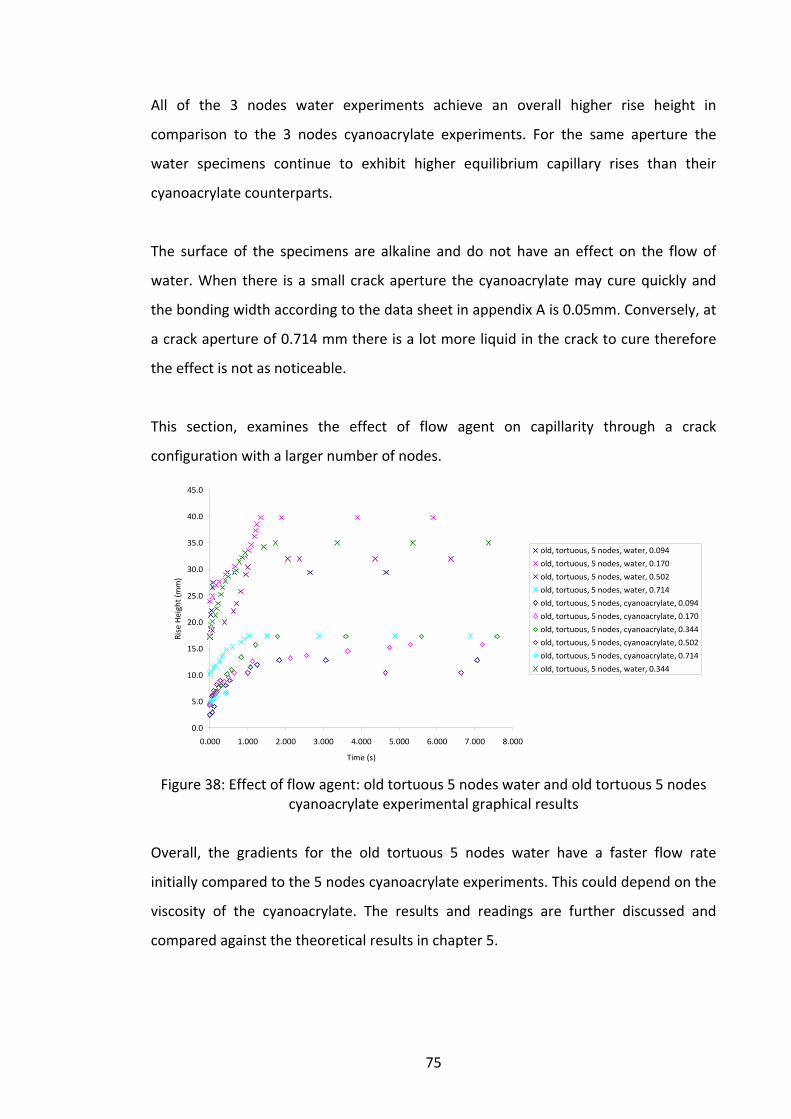
  75

All  of  the  3  nodes  water  experiments  achieve  an  overall  higher  rise  height  in 

comparison  to  the  3  nodes  cyanoacrylate  experiments.  For  the  same  aperture  the 

water  specimens  continue  to  exhibit  higher  equilibrium  capillary  rises  than  their 

cyanoacrylate counterparts.  

 

The  surface of  the  specimens are alkaline and do not have an effect on  the  flow of 

water. When  there  is a small crack aperture  the cyanoacrylate may cure quickly and 

the bonding width according to the data sheet in appendix A is 0.05mm. Conversely, at 

a crack aperture of 0.714 mm there is a lot more liquid in the crack to cure therefore 

the effect is not as noticeable.  

 

This  section,  examines  the  effect  of  flow  agent  on  capillarity  through  a  crack 

configuration with a larger number of nodes. 

0.0

5.0

10.0

15.0

20.0

25.0

30.0

35.0

40.0

45.0

0.000 1.000 2.000 3.000 4.000 5.000 6.000 7.000 8.000

Time (s)

Rise Height (mm)

old, tortuous, 5 nodes, water, 0.094

old, tortuous, 5 nodes, water, 0.170

old, tortuous, 5 nodes, water, 0.502

old, tortuous, 5 nodes, water, 0.714

old, tortuous, 5 nodes, cyanoacrylate, 0.094

old, tortuous, 5 nodes, cyanoacrylate, 0.170

old, tortuous, 5 nodes, cyanoacrylate, 0.344

old, tortuous, 5 nodes, cyanoacrylate, 0.502

old, tortuous, 5 nodes, cyanoacrylate, 0.714

old, tortuous, 5 nodes, water, 0.344

 Figure 38: Effect of flow agent: old tortuous 5 nodes water and old tortuous 5 nodes 

cyanoacrylate experimental graphical results  

Overall,  the  gradients  for  the  old  tortuous  5  nodes  water  have  a  faster  flow  rate 

initially compared to the 5 nodes cyanoacrylate experiments. This could depend on the 

viscosity  of  the  cyanoacrylate.  The  results  and  readings  are  further  discussed  and 

compared against the theoretical results in chapter 5.  

 

  76

Xanthan  gum  experimental  work  was  undertaken  to  compare  and  assess  the 

curing/hardening effect of cyanoacrylate during capillary flow experiments. Hence the 

change  in  viscosity  is  looked  at  in  detail  by  looking  at  the  fluids  used  in  the 

experimental work and seeing how capillary flow is affected. 

 

Xanthan  gum  was  measured  according  to  the  same  capillary  rise  height  for 

cyanoacrylate,  it has the same density and surface tension and contact angle but not 

necessarily the same viscosity. 

 

 

Figure 39: Effect of flow agent: Old planar xanthan gum, old planar water and old planar cyanoacrylate 

 Xanthan  gum  as  stated  in  chapter  3  is  a  biological  additive  that  has  no  setting 

characteristics  whereas  cyanoacrylate  does  cure  with  respect  to  time.  Therefore 

xanthan  gum  was  used  to  determine  the  difference  between  the  capillary  rise 

response  without  the  curing  effect.  The  xanthan  gum  additive  is  used  to  give 

equivalent  rise  heights  and  therefore  γ,  cosθ  and  ρ  same  as  cyanoacrylate  but  not 

necessarily  viscosity. As  cyanoacrylate  sets,  the  viscosity  increases  and  the  final  rise 

height  is  lower and comparing the final rise heights to the xanthan gum experiments 

the effect of cyanoacrylate curing is apparent through the lower rise heights. 

 

  77

The results displayed on the graph compare the rate of capillary rise height between 

cyanoacrylate and xanthan gum in order to establish the effect of cyanoacrylate curing 

in capillary rise. It can be seen that although cyanoacrylate and the xanthan gum used 

in  these experiments have been designed  to have  the same capillary rise height,  the 

cyanoacrylate  tests  overall  have  a  lower  equilibrium  rise  height  compared  to  the 

xanthan gum experiments. These  results and  readings  show  that  the  setting  time of 

the cyanoacrylate has a large effect on the overall rise height.  

 

 

Figure 40: Graph of capillary rise rates for xanthan gum, water and cyanoacrylate  

Looking at the videos and the graph gradients in figure 40 it is shown that the rate of 

rise is faster with the xanthan gum compared to cyanoacrylate. It can be seen that the 

water and the xanthan gum reach the same final rise height but not cyanoacrylate.  

 

The surface tension of the xanthan gum was calculated on the overall rise height  in a 

glass tube compared to the rise height in the same diameter tube with cyanoacrylate. 

As discussed previously  it  is known that the viscosity of a fluid does affect the overall 

rate of rise or rate of flow. Viscosity does not affect the level of rise height and in this 

instance  the  surface  tensions  could  be  different  as  those  were  not  calculated. 

Differences such as the  friction on the  inside of the glass tubes could differ affecting 

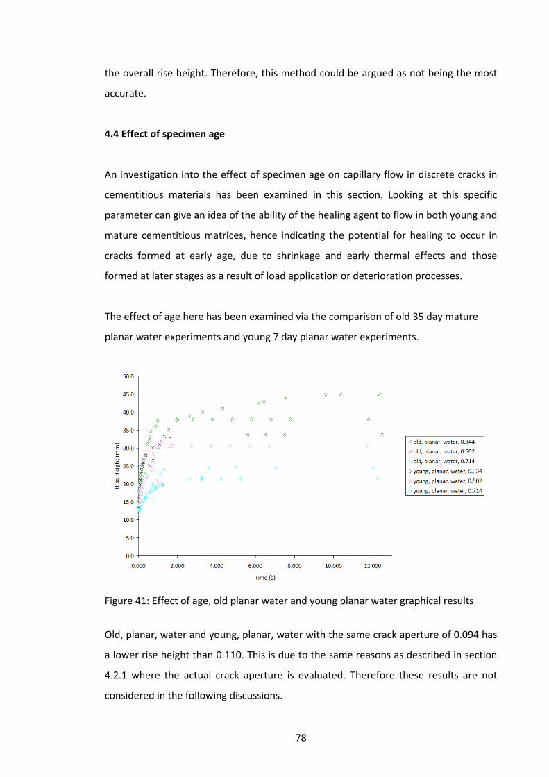
  78

the overall rise height. Therefore, this method could be argued as not being the most 

accurate. 

 

4.4 Effect of specimen age 

 

An investigation into the effect of specimen age on capillary flow in discrete cracks in 

cementitious materials  has  been  examined  in  this  section.  Looking  at  this  specific 

parameter can give an idea of the ability of the healing agent to flow in both young and 

mature cementitious matrices, hence  indicating  the potential  for healing  to occur  in 

cracks  formed  at  early  age,  due  to  shrinkage  and  early  thermal  effects  and  those 

formed at later stages as a result of load application or deterioration processes. 

 

The effect of age here has been examined via the comparison of old 35 day mature 

planar water experiments and young 7 day planar water experiments.  

 

 

Figure 41: Effect of age, old planar water and young planar water graphical results  

Old, planar, water and young, planar, water with the same crack aperture of 0.094 has 

a lower rise height than 0.110. This is due to the same reasons as described in section 

4.2.1 where  the  actual  crack  aperture  is  evaluated.  Therefore  these  results  are  not 

considered in the following discussions. 

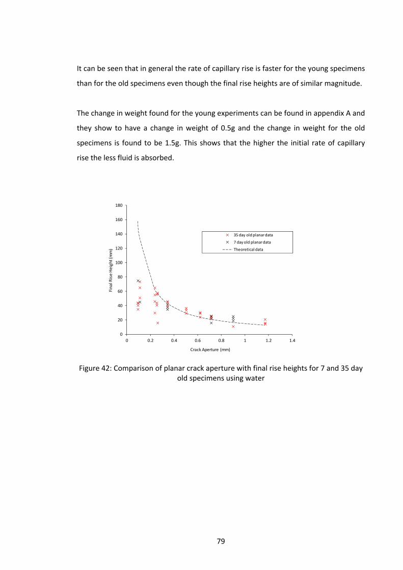
  79

 

It can be seen that in general the rate of capillary rise is faster for the young specimens 

than for the old specimens even though the final rise heights are of similar magnitude. 

 

The change in weight found for the young experiments can be found in appendix A and 

they  show  to have a  change  in weight of 0.5g and  the change  in weight  for  the old 

specimens  is  found  to be 1.5g. This shows  that  the higher  the  initial rate of capillary 

rise the less fluid is absorbed. 

 

0

20

40

60

80

100

120

140

160

180

0 0.2 0.4 0.6 0.8 1 1.2 1.4

Final Rise Height (mm)

Crack Aperture (mm)

35 day old planar data

7 day old planar data

Theoretical data

 

Figure 42: Comparison of planar crack aperture with final rise heights for 7 and 35 day old specimens using water 

 

 

 

 

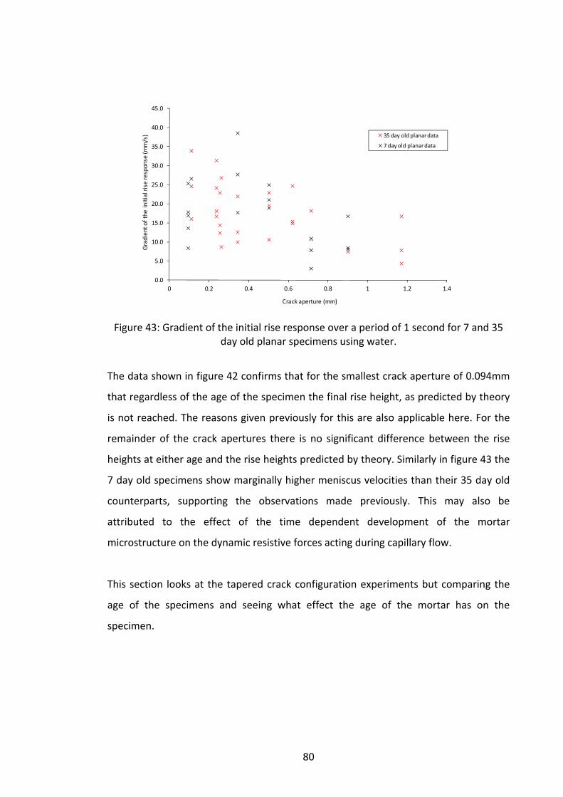
  80

0.0

5.0

10.0

15.0

20.0

25.0

30.0

35.0

40.0

45.0

0 0.2 0.4 0.6 0.8 1 1.2 1.4

Gradient of the

 initial rise response (m

m/s)

Crack aperture (mm)

35 day old planar data

7 day old planar data

 

Figure 43: Gradient of the initial rise response over a period of 1 second for 7 and 35 day old planar specimens using water. 

 

The data shown in figure 42 confirms that for the smallest crack aperture of 0.094mm 

that regardless of the age of the specimen the final rise height, as predicted by theory 

is not reached. The reasons given previously for this are also applicable here. For the 

remainder of  the  crack apertures  there  is no  significant difference between  the  rise 

heights at either age and the rise heights predicted by theory. Similarly in figure 43 the 

7 day old specimens show marginally higher meniscus velocities than their 35 day old 

counterparts,  supporting  the  observations  made  previously.  This  may  also  be 

attributed  to  the  effect  of  the  time  dependent  development  of  the  mortar 

microstructure on the dynamic resistive forces acting during capillary flow.  

 

This section  looks at  the  tapered crack configuration experiments but comparing  the 

age  of  the  specimens  and  seeing  what  effect  the  age  of  the  mortar  has  on  the 

specimen.  

 

  81

0.0

10.0

20.0

30.0

40.0

50.0

60.0

70.0

80.0

0.000 1.000 2.000 3.000 4.000 5.000 6.000 7.000 8.000

Time (s)

Rise Heigh

t (mm) old, tapered, water, 0.094‐0.110

old, tapered, water, 0.502‐0.714

old, tapered, water, 0.714‐0.9

young, tapered, water, 0.094‐0.170

young, tapered, water, 0.502‐0.714

young, tapered, water, 0.714‐0.900

 Figure 44: Effect of age: old tapered water and young tapered water 

 

Comparing the tapered experiments with the planar experiments, as  in figure 44, the 

young specimens have a  lower overall rise height than the old specimens. The  larger 

apertures  show  very  low  rise  heights,  as  previously  discussed  this  is  due  to  the 

methods undertaken  in experiments, where  the  first 12mm or so cannot be seen so 

therefore the overall rise height is not as accurate as it could be. 

 

Young  tapered water 0.094‐0.170 experiment has an  interesting  flow pattern. A  rise 

height of 30mm  is achieved within a second but  then  its maximum  rise height  takes 

another  3.5  seconds  to  reach maximum  rise  height.  The  video  shows  that  there  is 

absorption  through  the  cement  matrix  therefore  decreasing  the  overall  final  rise 

height. With the presence of a wire at this  location there  is a delay  in the rise height 

which is due to absorption taking place and then a subsequent increase in rise height. 

 

The effect of age using cyanoacrylate  is  looked at here to try and determine how the 

healing rates of cyanoacrylate are affected by age of cementitious materials. 

 

  82

0.0

5.0

10.0

15.0

20.0

25.0

30.0

0.000 1.000 2.000 3.000 4.000 5.000 6.000 7.000 8.000

Time (s)

Rise Height (mm)

old, planar, cyanoacrylate, 0.261

old, planar, cyanoacrylate, 0.344

old, planar, cyanoacrylate, 0.502

old, planar, cyanoacrylate, 0.714

young, planar, cyanoacrylate, 0.261

young, planar, cyanoacrylate, 0.344

young, planar, cyanoacrylate, 0.502

young, planar, cyanoacrylate, 0.714

 Figure 45: Effect of age: Old planar cyanoacrylate and young planar cyanoacrylate 

 

From figure 45, for old planar cyanoacrylate crack apertures of 0.261mm and 0.344mm 

the  overall  rise  height  is  higher  than  in  the  same  crack  apertures  for  the  young 

experiments. Looking at theory it would suggest that they should be at the same final 

height  but  having  looked  at  the  effect  of  age  in  the water  experiments  the  young 

specimens  absorb  less  therefore  the  cyanoacrylate  would  travel  further  up  the 

capillary. 

 

Old  planar  cyanoacrylate  and  young  planar  cyanoacrylate  specimens  have  similar 

overall  rise  heights  at  the majority  of  crack  apertures  considered,  as  confirmed  in 

figure 46. However, from figure 45 it can be also seen that they take a similar time to 

reach  the maximum  rise height. From  the experiments conducted  the  specimen age 

appears  to have  an effect on  the  rise  response; with older  specimens  retarding  the 

capillary rise response. This  is somewhat confirmed by the  initial rate of capillary rise 

data presented in figure 47. However, it is the longer timescale response of the system 

(1 to 8 seconds), as given in figure 45 that is a better reflection of this behaviour. This 

difference between the rise response of young and old specimens may be attributed to 

a change in the surface tension as a result of the age of specimen.  

 

 

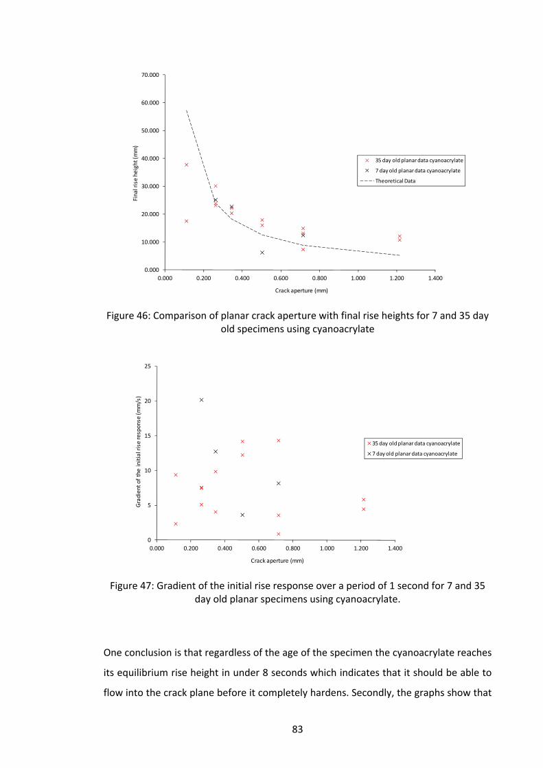
  83

0.000

10.000

20.000

30.000

40.000

50.000

60.000

70.000

0.000 0.200 0.400 0.600 0.800 1.000 1.200 1.400

Final rise height (m

m)

Crack aperture (mm)

35 day old planar data cyanoacrylate

7 day old planar data cyanoacrylate

Theoretical Data

 

Figure 46: Comparison of planar crack aperture with final rise heights for 7 and 35 day old specimens using cyanoacrylate 

0

5

10

15

20

25

0.000 0.200 0.400 0.600 0.800 1.000 1.200 1.400

Gradient of the

 initial rise response (m

m/s)

Crack aperture (mm)

35 day old planar data cyanoacrylate

7 day old planar data cyanoacrylate

 

Figure 47: Gradient of the initial rise response over a period of 1 second for 7 and 35 day old planar specimens using cyanoacrylate. 

 

 

One conclusion is that regardless of the age of the specimen the cyanoacrylate reaches 

its equilibrium rise height in under 8 seconds which indicates that it should be able to 

flow into the crack plane before it completely hardens. Secondly, the graphs show that 

  84

even though curing occurs the fluid still continues to flow afterward, not reaching the 

maximum rise height but flowing further. 

 

The  influence  of  specimen  age  on  the  capillary  rise  response  of  cyanoacrylate  in 

tapered crack  configurations are evaluated here, and  the  results presented  in  figure 

48. 

 

0.0

10.0

20.0

30.0

40.0

50.0

60.0

0.000 1.000 2.000 3.000 4.000 5.000 6.000 7.000 8.000

Time (s)

Rise Height (mm)

old, tapered, cyanoacrylate, 0.094‐0.110

old, tapered, cyanoacrylate, 0.502‐0.714

young, tapered, cyanoacrylate, 0.094‐0.110

young, tapered, cyanoacrylate, 0.502‐0.714

 Figure 48: Effect of Age: Old tapered cyanoacrylate and young tapered cyanoacrylate  

It  takes  a  significant  amount  of  time  for  the  old  tapered  experiments with  a  crack 

aperture of 0.094 – 0.110 as it is still rising at the end, as demonstrated in figure 48. As 

there  are  significant  differences  in  the  gradients  throughout  the  rise  height  the 

experiments do not show  that  it  is possible  for  the cyanoacrylate  to set at  the point 

when full maximum rise height is achieved. The young experiments show that only half 

of the old maximum rise height is achieved. Looking at larger aperture, 0.714mm and 

0.900mm  the effect of age on  the capillary rise  is negligible. This  is as  the  larger  the 

aperture,  the  lower  the  rise height  so  therefore  the  less overall absorption  into  the 

cement matrix. Therefore,  it  is assumed  that  there  is unhydrated cement  in younger 

specimens and therefore more fluid flow  into the cement matrix reducing the overall 

capillary flow. When there is a larger crack aperture the capillary rise is anticipated to 

be  lower, providing a smaller area over which absorption  into the cement matrix can 

occur and therefore  less absorption  into the cement matrix, hence why the values of 

old and young are of similar magnitude. 

  85

4.5 Effect of specimen saturation  

 

Flow  in  discrete  cracks  in  saturated  concrete  is  an  important  area  to  look  at  as 

structures rarely are in a moisture free state in outdoor environments. 

 

0.0

5.0

10.0

15.0

20.0

25.0

30.0

35.0

0.000 2.000 4.000 6.000 8.000 10.000 12.000 14.000

Time (s)

Rise Height (mm)

old, planar, water, unsaturated, 0.620

old, planar, water, unsaturated, 0.714

old, planar, water, unsaturated, 0.900

old, planar, water, saturated, 0.620, 1

old, planar, water, saturated, 0.620, 2

old, planar, water, saturated, 0.714, 1

old, planar, water, saturated, 0.714, 2 

old, planar, water, saturated, 0.900, 1

old, planar, water, saturated, 0.900, 2 

 Figure 49: Effect of specimen saturation old planar water saturated and unsaturated  

Results in figure 49 show that there is no significant difference between the results for 

the  saturated  and  unsaturated  specimens.  It  could  be  assumed  that  the  saturated 

specimens would overall have a higher rise height than the unsaturated specimens as 

no fluid would be absorbed into the cement matrix either side of the crack plane.  

 

Differences  previously  found  in  data  show  that with  low  absorption  of  fluid  into  a 

specimen  the  capillary  rise  height  is  higher  than  that  of  high  absorption.  Images  in 

figure 35 show that the water does absorb  into the matrix. This therefore must have 

significance on the overall rise height potentially decreasing the maximum achievable 

rise heights. 

 

Looking at capillary rise for saturated and unsaturated, data shows that saturated flow 

is slower than for unsaturated specimens. This shows that the attractive forces need to 

develop between the flow agent and the capillary wall to enable the fluid to rise. The 

development  of  these  forces would  be  disrupted  by  the  presence  of water  on  the 

boundary therefore a reduced capillary driving force. 

  86

4.6 Main concluding results 

 

Below the equivalent planar crack aperture for natural cracks and the effectiveness of 

cyanoacrylate  to heal has been  investigated. This has been  completed  to determine 

how  reliable  the  experimental  work  would  be  to  determine  flow  through  natural 

cracks in concrete. 

 

4.6.1 Equivalent planar crack for natural cracks 

 

 

Figure 50: Comparison of natural cracks for planar cracks 

 

Comparisons between natural crack rise height and planar crack rise heights have been 

made  to  determine  the  reliability  of  results.  Therefore,  in  future  fluid  flow  can  be 

determined for all healing agents with natural cracks based on planar experiments. 

 

Figure 50 clearly shows  that  the natural crack  flow  is considerably  lower  than planar 

fluid flow. There  is a clear correlation between the change  in rise height for a natural 

crack  and  a  planar  crack  for  all  crack  apertures.  Taking  forward  this  information  a 

relationship between a natural  crack aperture and a planar  crack  rise height  can be 

determined. 

 

  87

0

0.1

0.2

0.3

0.4

0.5

0.6

0.7

0.8

0 0.1 0.2 0.3 0.4 0.5 0.6 0.7 0.8

Natural crack aperture (mm)

Planar crack ape

rture (m

m)

 

Figure 51: Graph of planar crack aperture compared to natural crack aperture 

 

The  rise  heights  for  a  series  of  natural  cracks  have  been  examined  to  determine 

whether  it  is possible to predict the capillary rise height for a natural crack of known 

aperture  using  an  equivalent  planar  aperture  in  equation  5.1.  The  relationship 

between capillary  rise  in natural cracks and  in an equivalent planar crack  is given  in 

figure 51. The relationship is of linear form and demonstrates that as the natural crack 

aperture  increases,  the  effect  of  the  crack  tortuosity  and  crack  surface  roughness 

decreases until there  is no observed difference between a natural crack and a planar 

crack. According to the experiments this appears to happen at a crack aperture greater 

than 0.3mm. However, without further investigation using wider apertures it is difficult 

to conclude whether this limit is accurate. This method can be used to determine any 

property  for  fluid  flow  through  a  natural  crack  using  the  properties  of  fluid  flow 

through a planar crack. 

 

 

 

 

 

 

 

 

  88

Table 9: Crack aperture calculation 

Crack width Natural Crack  

(mm) 

Final rise height for natural crack (mm) 

Equivalent planar crack aperture  (mm) 

0.170  37.5  0.390 0.344  23.3  0.450 0.714  14.2  0.738 

 

4.6.2 Effectiveness of cyanoacrylate flow and potential to heal 

 

Experiments using  cyanoacrylate  show  a  general  trend  that  the  initial  rate of  rise  is 

quicker than that of water. Therefore, if a rapid heal is needed a healing agent with the 

same viscosity as cyanoacrylate should be used instead of one with a lower viscosity. 

 

Other  experimental  results  and  readings  show  that  the  younger  specimens  tend  to 

absorb more  healing  agent  into  the  cement matrix.  Therefore  for  rapid  healing  in 

cracks  in  cementitious materials,  a  young  specimen with  a  crack  aperture  less  than 

0.5mm (as this is the bonding width of cyanoacrylate used) would be recommended. 

 

4.7 Summary of conclusions 

 

Research  in this  thesis has been completed by  looking at different variables  that can 

affect capillarity in cementitious materials. The key conclusions from the experimental 

work  and  data  are  listed  below  and  how  they  can  be  applied  to  self  healing 

mechanisms in cementitious materials is described. 

• Crack aperture affects the overall rise height, with higher rise heights observed 

from smaller crack apertures as predicted by theory. However, the capillary rise 

height from natural crack apertures does not reach its theoretical value from all 

crack apertures examined. This may be due to surface roughness of the crack 

face or the change  in surface tension as a result of the addition of fluorescein 

to the water.  

• Results confirm that crack configuration does vary the rate of fluid rise height 

depending on the crack inclination. Therefore, to determine the fluid flow of a 

  89

healing agent through cementitious materials the crack geometry would need 

to be examined to allow the rate of capillary flow to be determined.  

• The flow agent used experimentally does have an effect on the rate of rise due 

to  its viscosity and using equation 5.1 only an approximation on how  far  the 

fluid will travel can be made. 

• The degree of saturation and the age of the specimen only had an effect on the 

rate of capillary  rise and not on  the  final  level of capillary  rise observed. This 

indicates  that  along  with  the  degree  of  saturation  and  specimen  age  the 

healing potential of the self healing cementitious material will be dependant on 

the curing rate of the healing agent and its ability to flow into the crack before 

hardening. 

• Experiments  show  that  healing  with  cyanoacrylate  occurs  in  a  matter  of 

seconds  with  a  crack  width  less  than  0.502mm.  This  indicates  that  natural 

cracks with a crack aperture  less  than 0.502mm can be successfully healed  in 

autonomic  healing  systems.  This  was  seen  post  experiment  when  the 

specimens with this crack width and below had successfully bonded. 

• There  appears  to  be  a  relationship  between  the  final  capillary  rise  height 

measured for natural cracks and the final capillary rise height predicted for an 

equivalent planar crack. For a crack aperture less than 0.5mm, the relationship 

between natural and planar crack apertures  is not  linear and  therefore more 

experimental work would need  to be undertaken  to determine  the nature of 

this relationship more accurately. However, it is shown that for crack apertures 

greater  than 0.5mm a  linear relationship  is observed so  therefore  if a natural 

crack  aperture  is  known  the  fluid  rise  through  that  crack  can be determined 

based on a planar crack simulation.  

90 

Chapter 5 

Theory and Validation of Experimental Results 

 

 

 

5. 1 Basic capillary flow equations  

 

Liquid flow against gravity through a capillary or narrow space, such as a thin tube,  is 

known by capillary action or capillarity.  

Capillary  flow  occurs  due  to  the  intermolecular  forces  between  liquids  and  solid 

surrounding surfaces. As explained in Chapter 2, capillarity is caused by the joint action 

of the  fluid surface tension and the adhesion between the fluid and the solid wall of 

the capillary.  

The adhesion pulls  the  liquid  column up until  there  is a  sufficient mass of  liquid  for 

gravitational forces to overcome the intermolecular forces. The contact length (around 

the edge) between  the  top of  the  liquid column and  the  tube  is proportional  to  the 

diameter  of  the  tube, while  the weight  of  the  liquid  column  is  proportional  to  the 

square of the tube's diameter, so a narrow tube will draw a liquid column higher than 

a wide tube.  

The height z of a liquid column is given by; 

grz

ρθγ cos2

=                   (5.1) 

91 

 

Figure 52: Image of a capillary demonstrating the capillary action formula (Young 2004) 

where   is the liquid‐air surface tension in N/m, θ is the angle that the meniscus forms 

with crack/solid face in degrees, ρ is the density of liquid in kg/m3, g is the force due to 

gravity acting on the fluid in the capillary in m/s2, and r is radius of the capillary in mm 

and μ is the dynamic viscosity in Ns/m2. 

 

5.2 Analysis of the Lucas‐Washburn equation 

 

The  Lucas‐Washburn equation  (L‐W)  (Hamraoui  and Nylander. 2002)  given below  in 

equation  5.2,  describes  the  dynamic  flow  of  liquid  in  a  capillary  tube.  The  forces 

considered  in  the  equation  are  the  inertia,  surface  tension  (adhesion),  gravity,  and 

dynamic viscosity. 

 

ttztztgzrr

ttztz

tr

∂∂

−−=⎟⎠⎞

⎜⎝⎛

∂∂

∂∂ )()(8)()cos(2)()( 22 πμρπθγπρπ     (5.2) 

 

Where t is the time in seconds. 

 z 

 θ 

 r 

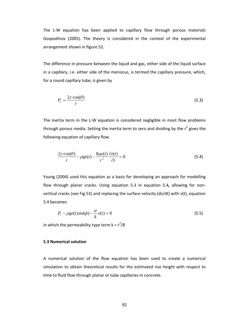
92 

The  L‐W  equation  has  been  applied  to  capillary  flow  through  porous  materials 

Gospodinov  (2005).  The  theory  is  considered  in  the  context  of  the  experimental 

arrangement shown in figure 52. 

 

The difference in pressure between the liquid and gas, either side of the liquid surface 

in a capillary,  i.e. either side of the meniscus,  is termed the capillary pressure, which, 

for a round capillary tube, is given by  

 

rPc

)cos(2 θγ=                 (5.3) 

 

The  inertia  term  in  the L‐W equation  is considered negligible  in most  flow problems 

through porous media. Setting the inertia term to zero and dividing by the r2 gives the 

following equation of capillary flow. 

 

0)()(8)()cos(22 =

∂∂

−−ttz

rtztgz

rμρθγ

          (5.4) 

 

Young (2004) used this equation as a basis for developing an approach for modelling 

flow  through  planar  cracks.  Using  equation  5.3  in  equation  5.4,  allowing  for  non‐

vertical cracks (see Fig 53) and replacing the surface velocity (dz/dt) with v(t), equation 

5.4 becomes 

0)()sin()( =−− tvk

tgzPcμφρ             (5.5) 

In which the permeability type term k = r2/8 

 

5.3 Numerical solution 

 

A  numerical  solution  of  the  flow  equation  has  been  used  to  create  a  numerical 

simulation  to obtain  theoretical  results  for  the estimated  rise height with  respect  to 

time to fluid flow through planar or tube capillaries in concrete. 

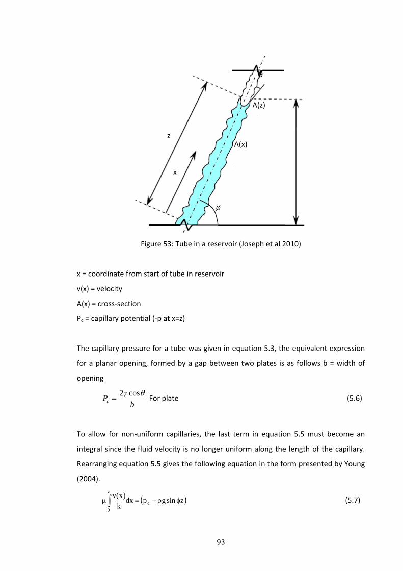
93 

 

Figure 53: Tube in a reservoir (Joseph et al 2010) 

 

x = coordinate from start of tube in reservoir 

v(x) = velocity 

A(x) = cross‐section 

Pc = capillary potential (‐p at x=z)       

 

The capillary pressure for a tube was given in equation 5.3, the equivalent expression 

for a planar opening,  formed by a gap between two plates  is as  follows b = width of 

opening 

bPc

θγ cos2=  For plate               (5.6)  

 

To  allow  for non‐uniform  capillaries,  the  last  term  in equation 5.5 must become  an 

integral since the fluid velocity  is no  longer uniform along the  length of the capillary. 

Rearranging equation 5.5 gives the following equation in the form presented by Young 

(2004).  

( )zsingpdxk

)x(vc

z

0

φρ−=μ∫               (5.7) 

A(x)

θ 

z

A(z) 

x

Ø 

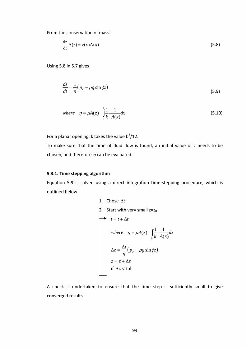
94 

From the conservation of mass: 

)x(A)x(v)z(Adtdz

=                 (5.8) 

 

Using 5.8 in 5.7 gives 

 

( )zgpdtdz

c φρη

sin1−=

              (5.9) 

dxxAk

zAwherez

∫=0 )(

11 )( μη             (5.10) 

 

For a planar opening, k takes the value b2/12. 

To make  sure  that  the  time of  fluid  flow  is  found,  an  initial  value of  z needs  to be 

chosen, and therefore η can be evaluated. 

 

5.3.1. Time stepping algorithm 

Equation  5.9  is  solved  using  a  direct  integration  time‐stepping  procedure, which  is 

outlined below 

1. Chose  tΔ  

2. Start with very small z=z0 

ttt Δ+=  

dxxAk

zAwherez

∫=0 )(

11 )( μη  

( )

tolz if

sin

<ΔΔ+=

−Δ

=Δ

zzz

zgptz c φρη

 

 

A  check  is  undertaken  to  ensure  that  the  time  step  is  sufficiently  small  to  give 

converged results. 

 

 

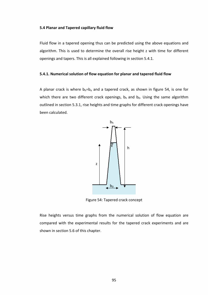
95 

5.4 Planar and Tapered capillary fluid flow 

 

Fluid flow  in a tapered opening thus can be predicted using the above equations and 

algorithm. This  is used  to determine  the overall  rise height  z with  time  for different 

openings and tapers. This is all explained following in section 5.4.1. 

 

5.4.1. Numerical solution of flow equation for planar and tapered fluid flow 

 

A planar crack  is where bh=bo and a  tapered crack, as shown  in  figure 54,  is one  for 

which  there  are  two  different  crack  openings,  bh  and  b0. Using  the  same  algorithm 

outlined in section 5.3.1, rise heights and time graphs for different crack openings have 

been calculated. 

 

 

Figure 54: Tapered crack concept 

 

Rise  heights  versus  time  graphs  from  the  numerical  solution  of  flow  equation  are 

compared with  the  experimental  results  for  the  tapered  crack  experiments  and  are 

shown in section 5.6 of this chapter. 

 

 

 

 

h 

z 

     bh 

     b0 

96 

5.5 Validation of the numerical model 

 

The  numerical  solution  involves  using  an  explicit  time  stepping  solution  of  the 

temporal  equation.  Convergence  with  respect  to  the  time  step  was  checked  by 

reducing the step size until the predicted responses did not change by more than 1% 

with a halving of the time step.  

 

Specifically, the solutions presented used a time step size of 0.0001s and if reduced to 

0.00005s the predicted responses would be  indistinguishable from each other on the 

numerical simulations shown. 

 

In  order  to  establish  the  generalised  response  of  the  system,  the  capillary  flow  of 

water predicted by equation 5.9,  in two different glass capillary tubes of 0.3mm and 

1.0mm  diameter,  is  compared  to  that  predicted  by  the  standard  Lucas Washburn 

equation.  

 

The standard Lucas Washburn response was obtained by the numerical integration of 

equation 5.9. However, the numerical response, thus calculated, was checked against 

the analytical expression given by Fries and Dreyer  (2008), with  the  results  from  the 

two  calculations being  the  same  to within  the precision of  the  calculation  and  thus 

indistinguishable from each other on graphs in figure 55. 

 

97 

Figure 55: Validation of numerical model with analytical solution 

 

Experimental  validation  of  the  numerical model was  performed  using  capillary  rise 

data recorded by Liou et al. (2009) for water in a glass capillary tube of known internal 

diameter. The parameters used to simulate the experimentally observed capillary rise, 

as  reported by Liou et al. were  γ = 0.070 N/m, θ = 30° ρ = 1000kg/m3 and µ= 0.001 

Ns/m2. Good agreement between the experimental data and the numerical solution is 

observed for a capillary diameter of 0.1mm, as shown  in figure 56. Also presented  in 

Figure  56  is  the  rate  of  capillary  rise  calculated  using  the  analytical  solution  to  the 

Lucas Washburn equation from Fries and Dreyer (2008). 

 

98 

 

Figure 56: Validation of numerical model with experimental data from Liou et al. 

(2009) 

 

5.6 Validation of experimental results with theory 

 

This section of the thesis considers the experimental results presented in Section 4 and 

compares them with numerical flow simulations such that the validity of the model 

and results can be determined. 

 

5.6.1 Planar fluid flow 

 

In this section results for planar experiments described in chapter 4 are compared with 

those obtained from the numerical model described above.  

 

5.6.1.1 Planar fluid flow water 

 

Figure 57 displays results the experimental and numerical results for a crack aperture 

of 0.502mm. 

99 

 

0.0

5.0

10.0

15.0

20.0

25.0

30.0

35.0

40.0

45.0

0.000 2.000 4.000 6.000 8.000 10.000 12.000 14.000 16.000

Time/s

Rise Height/mm

Experimental, 0.502

Numerical, 0.502

  

Figure 57: Experimental and numerical results for mature, planar, water with a crack 

aperture of 0.502mm 

 

The  graph  shows  that  the  difference  between  the  experimental  and  numerical 

response  is quite  large both  in  terms of capillary  response  time and equilibrium  rise 

height. However this could be due to a number of reasons.  

 

As discussed  in chapter  four,  the point  taken  from  the graph  starts  from 12mm  rise 

height and the time is a time not equal to zero seconds so therefore what is shown by 

the experimental  results  is not a  full evaluation of capillary  flow. However,  the data 

has been  corrected by  alteration of  the origin  and  the numerical  results have been 

compared with these correct data.  

 

The crack aperture also has shown  to vary quite significantly  in Chapter 4 which will 

have also affected the overall final capillary rise height and rate of rise. 

 

5.6.1.2 Planar fluid flow cyanoacrylate 

 

Planar fluid flow of cyanoacrylate has been considered in this section with a numerical 

solution of the flow equation, presented in Appendix D.  

100 

 

The next topic discussed is how the surface tension and contact angle of cyanoacrylate 

were determined. These properties were measured as they are a fundamental element 

of the equation of capillary flow.  

 

The contact angles were measured directly from images of the liquid meniscus within a 

glass capillary tube, as illustrated in Fig 58.  

 

The  image  in  figure  58  shows  the measured  contact  angle  for  cyanoacrylate having 

risen  in  a  tube of  radius, 0.315mm,  an overall distance  z, of  15.96mm.  The  contact 

angle between the meniscus of the cyanoacrylate and the tube was measured as 38˚. 

Three different tubes all of the same radius were used to calculate contact angles and 

an average value calculated. It was this average value that was used for the numerical 

simulations. 

 

Figure 58: Capillary tube of radius, 0.315mm with a contact angle of 38˚ 

 

Equation 5.1 has been used to determine the surface tension. If it is rearranged, the 

surface tension can be calculated with it being the subject of the equation (equation 

5.11); 

 

101 

)(cos2 θργ grz

=                   (5.11) 

The  model  also  requires  the  viscosity.  However,  since  the  curing  time  for  the 

cyanoacrylate is relatively short it was considered important to determine the change 

in dynamic viscosity over the duration of a test. Figure 59 shows that the flow changes 

dramatically for old, planar, cyanoacrylate with a crack aperture of 0.502mm.  

 

       

 Figure 59: Image of capillary tube and theoretical graph of rise height, z versus time, t  

For a thin capillary tube the viscosity can be calculated by considering equation 5.9 at 

time  t  over  a  time  interval  t1  to  t2  noting  that  Δt=t2‐t1  .  In  this  discretized  form, 

equation 5.9 becomes: 

 

))2

(( 2112 zzpgpk

tzz

c+

−−=−

μΔ            (5.12) 

 

Rearranging equation 5.12 for the viscosity gives: 

))2

(( 21

12

zzpgp

zztk c

+−

−−=

Δμ             (5.13) 

 

 

 

 

h 

z 

z Δ t

z1 Δz z2 

t1    t    t2 t

2

102 

Table 8: Calculation of viscosity 

Point  g (m/s2) 

Change in time (s) 

k (mm2x10‐8) 

r (mm) 

θ (˚)

Surface tension 

γ (N/m) 

pc (N) 

μ  (Ns/m2 x10‐3)

1  9.81  0.040  2.1 0.000502 39 0.032  0.099  0.2142  9.81  0.048  2.1 0.000502 39 0.032  0.099  0.2393  9.81  0.088  2.1 0.000502 39 0.032  0.099  0.2364  9.81  3.000  2.1 0.000502 39 0.032  0.099  117.8

 

Results for the case of a planar crack  in mature concrete for an opening of 0.502mm 

were  computed  for  the  following  three  time  intervals  0.016s  to  0.056s,  0.088s;  to 

0.136s and 1.232s to 1.320s. These results are summarised in Table 8. 

 

Figure 60 shows the experimental and the numerical graphical results for capillary flow 

of cyanoacrylate through a planar crack. 

 

0.0

5.0

10.0

15.0

20.0

25.0

0.000 1.000 2.000 3.000 4.000 5.000

Time (s)

Rise Height (mm)

old planar cyanoacrylate experimental0.502

old planar cyanoacrylate numerical 0.502

 

Figure  60:  Experimental  and  numerical  results  for  old,  planar,  cyanoacrylate with  a crack aperture of 0.502mm.     

It  is  evident  that  yet  again  there  is  a  difference  in  final  rise  height  between  the 

numerical and experimental  results and  readings. An overall difference between  the 

103 

two  is approximately 6mm. This yet again could be due  to  the changes  in  the  initial 

point of measurement as spoken about previously. 

 

5.6.2 Tapered fluid flow 

 

Fluid flow in a tube or crack where b0 is not equal to bh can be defined as tapered flow. 

The next two  following sections take results  from the results chapter 4 and compare 

them to the numerical values created with the numerical solution given in Appendix D.  

 

5.6.2.1 Tapered fluid flow water 

 

This  section  discusses  the  differences  found  between  the  numerical  and  the 

experimental models for tapered fluid flow in mortar specimens. 

 

0.0

5.0

10.0

15.0

20.0

25.0

30.0

35.0

40.0

45.0

0.000 1.000 2.000 3.000 4.000 5.000

Time (s)

Rise Height (mm)

old tapered water experimental 0.344‐0.502

old tapered water numerical 0.344‐0.502

 

Figure  61: Old,  tapered, water  0.344‐0.502mm  crack  aperture  for  experimental  and numerical work  

Figure 61 presents the numerical and the experimental results graphically so that the 

difference between flow rates can be looked at in detail. 

 

The  rates  of  flow,  i.e.  the  gradient  for  each  of  the  experiments,  are  shown  to  be 

somewhat  similar.  Therefore,  the  numerical model  validates  the  flow  rate  is  at  a 

104 

similar value to that of the experimental. It can be seen that the final rise heights are 

also in a similar region of value. The differences could be based on how absorption into 

the cement matrix is not taken into consideration in the model which would affect the 

overall final rise height by a significant amount. There is still evidence, in figure 61, that 

additional simulations and amendments are required to accurately model the capillary 

rise response.  

 

5.6.2.2 Tapered fluid flow cyanoacrylate 

 

Here capillary  flow  is assessed with cyanoacrylate as  the  flow agent  in experimental 

and numerical work is looked at in detail. 

0.0

5.0

10.0

15.0

20.0

25.0

30.0

0.000 1.000 2.000 3.000 4.000 5.000

Time (s)

Rise Height (mm)

old tapered, cyanoacrylate experimental0.344‐0.502

old tapered cyanoacrylate numerical 0.344‐0.502

 Figure 62: Old, tapered, cyanoacrylate 0.344‐0.502mm crack aperture for experimental and numerical work  

Similarly to tapered  fluid  flow of water as to tapered  fluid  flow of cyanoacrylate, the 

gradient  from  0‐1  seconds  are  similar,  indicating  that  the  numerical  solution 

represents the experimental results and readings properly 

 

 

 

 

 

105 

5.7 Conclusions  

 

The theory in this chapter gives the correct general behaviour. However, further work 

would be needed to explore the capillary and resistance forces active in this system in 

order  to  derive modifications which would  allow  the  experiments  to  be  simulated 

accurately. 

 

It  is  evident  that  the  experimental  rise  heights  are  lower  than  the  theoretical  rise 

heights. Results also  show  that  the  standard  Lucas‐Washburn  theory over estimates 

the rate and rise height for capillary flow.  

  106

Chapter 6 

Conclusions and further work 

 

 

6.1 Introduction 

 

The work  reported  in  this  thesis endeavoured  to examine  some of  the  factors 

which affect capillarity through cementitious materials. 

 

The main objectives of  this  study were detailed  in Chapter 1. These objectives 

covered  four areas of  investigation and these were detailed  in chapter 4 which 

analyse the experimental results: 

 

1. Effect of crack configuration 

2. Effect of flow agent 

3. Effect of specimen age  

4. Effect of specimen saturation 

 

A detailed review of relevant literature was presented in Chapter 2 and Chapter 

5 presented observations made based on  the numerical models  relating  to  the 

experimental work.  This comes under the section 5.6 Validation of experimental 

results. 

 

6.2 Conclusions 

 

The conclusions  from each of  the  investigations have been given at  the end of 

the results chapter. However, a summary of the conclusions is presented here. 

 

 

 

 

  107

6.2.1 Capillary flow experimentation and conclusions 

 

The  conclusions  in  Chapter  four  state  that  although  the  overall  experimental 

procedures were successful  for producing some  results and  readings, however, 

there are a few issues that could be resolved and are listed below: 

 

• Chapter  4  shows  that  the data on  the  graphs  starts  recording  capillary 

flow mid  flow.    It  is hard  to determine when  capillary  rise  through  the 

different crack configurations starts.  This is due to the time at which the 

fluid is poured into the tray and also determining the actual rise height by 

where capillary action starts.   One way to overcome these  issues would 

be to either use a clear scale, where the markings could still be seen and 

also  raising  the  specimen  having  the  fluid  reservoir  at  the  base  of  the 

specimen so full capillary flow can be captured.   Therefore, the capillary 

action  can  be monitored  initially  from  0  and  a  full  capture  of  capillary 

flow can be determined. 

 

6.2.2 Effect of crack configuration 

 

The effect of crack configuration on capillary rise response is one of the variables 

that has been  looked at  in detail  in  this  thesis.   Simulations of planar,  tapered, 

tortuous and natural cracks are looked at. 

 

• The general trends in the results show that after experimentation where 

there  is a  large change  in weight  there  is a  lower overall maximum  rise 

height achieved for that particular crack aperture. 

• Some  results  and  readings  show  that  using  formula  5.1  demonstrating 

capillary  flow  that  the  expected  rise  height  for  a  crack  aperture,  the 

maximum rise height  is considerably  less.   This may be attributed to the 

actual crack aperture being larger than anticipated. 

  108

• Results  do  show  some  validity  as  the  natural water  experiments  show 

consistency with theory that the greater the crack width of the capillary 

the lower the overall rise height.   

• Unlike the planar or tapered experiments where there  is a smaller crack 

width, it takes longer for fluid flow to reach the maximum rise height; the 

natural experiments do not display any significant difference  in the time 

taken to achieve maximum rise height. 

• Results do not  show  significant changes  in overall maximum  rise height 

for capillary flow for the 3 nodes and 5 nodes tortuous experiments.   

 

 

6.2.3 Effect of flow agent 

 

Looking at how flow agents affect capillarity with the changes in surface tension 

and viscosity  is an area that has been discussed and explored  in chapter 4.   The 

key conclusions from the results are presented below: 

 

• Fluid  flow  of  water  shows  to  have  on  the  whole  a  larger  rate  of 

progression  through  the  simulated  capillaries  compared  to 

cyanoacrylate.    This  can  be  attributed  to  the  low  interaction  of water 

with the surfaces together with lower viscosity. 

• Cyanoacrylate in the results shows that through capillary flow that there 

is  a  significant  change  in  the  overall maximum  rise  height,  due  to  the 

curing effect that cyanoacrylate has when it comes into contact with air. 

• However, when cyanoacrylate  is compared to xanthan gum, a fluid with 

the  same  density  and  surface  tension  properties  of  cyanoacrylate  but 

without  the  curing  effect,  it  can  be  seen  that  a  higher maximum  rise 

height is achieved. 

 

 

 

  109

6.2.4 Effect of specimen age 

 

Specimen  age  is  another  area  of  experimentation  that  has  been  looked  at  in 

detail and yet again the key conclusions presented here: 

 

• Results  from  experimental  work  comparing  mature  and  young 

specimens  show  that  higher  capillary  flow  is  achieved  for  both 

cyanoacrylate and water in mature specimens.   

• For  the  healing  agent  to  penetrate  far  into  the  cracks  of  cracked 

concrete specimens,  it  is therefore concluded that fluid flow of healing 

agents in mature specimens is better than that in young specimens.  

• Comparisons between old and young mortar specimens show that rates 

of  rise  are  faster  in  mature  mortar  specimens  than  young  mortar 

specimens.   This can be attributed to  less fluid being absorbed  into the 

cement matrix of a mature specimen. 

• Younger  specimens  show more  fluid  being  absorbed  into  the  cement 

matrix therefore is good for early age healing. 

 

6.2.5 Effect of specimen saturation 

 

Results  and  readings  in  saturated  experiments  show  that  there  is  not  a  large 

difference  in  overall  rise  heights  for  saturated  or  unsaturated  specimens.  

Therefore  in the context of how far fluid flows  in specimens that need to  ‘heal’ 

the cracks there would not be a difference  in how far the fluid travels based on 

saturation. 

 

6.3 Numerical models and validity of results 

 

The  conclusions  for  the  numerical  solutions  based  on  flow  through  cracks  are 

stated here.   Each separate solution and the validity of the results presented  in 

section 5.6 are also touched on. 

  110

 

The numerical solutions of planar and tapered flow are successful in that for any 

crack  aperture,  flow  agent;  graphical  results  of  final  rise  heights  and  capillary 

pore pressures are calculated based on the theory presented through the work 

of Young (2004). 

 

However, due  to  the problems occurring of  the origins of  the graphical  results 

produced  from  experimental  work,  comparing  these  with  the  numerical 

simulation graphical has not been very  successful.   There are many  issues  that 

could  affect  the  results produced  through  the  numerical  solutions.    These  are 

listed below: 

 

• The angle of crack  inclination, viscosity of cyanoacrylate and the contact 

angles for each flow agent used have been calculated experimentally and 

are not values that the solutions can depend on.   

• This is as the experimental values could potentially show some inaccuracy 

and would therefore affect the numerical simulation of flow. 

• These issues are reflected in chapter 5.6 were the validity of the results is 

discussed more in depth. 

 

6.4 Recommendations for further work 

 

There are many areas that have been touched upon in Chapter 2 where all of the 

gaps have been noted throughout literature.  Chapters 3 – 5 state how the work 

completed  in  this  thesis has endeavoured  to  address  the  shortcomings of  this 

particular research field. 

 

Even  though  the  gaps  have  been  looked  at  and  ways  to  overcome  areas  in 

research filled there are some areas that could be built upon experimentally and 

numerically. 

 

  111

Ideas for further work are presented below  looking  individually at experimental 

and numerical studies: 

 

• In this study only two flow agents have been used.  Therefore it would be 

beneficial to use a  larger variety of flow agents with different properties 

such as surface tension and viscosity. 

• Other fluids that have been found to be used more in practise are epoxy 

resins, PFA  in solution and GGBS  in solution.   Therefore,  these could be 

used  to  investigate  flow  properties  of  other  healing  agents  through 

cementitious materials. 

• Models of sinusoidal capillaries simulated by Gospodinov (2005) simulate 

different crack apertures of capillaries of varying tortuosity.   A potential 

for  further  experimentation  could  be  creating  different  types  of 

capillaries to compare them with the numerical solutions.   

• Joseph et al.’s work (2009) spoken about in Chapter 2, show that natural 

cracks  of  similar magnitude  are  looked  at  for  one  type  of  flow  agent.  

Therefore to examine more crack apertures for natural experiments and 

to find an experimental procedure where the fluid front of cyanoacrylate 

can be detected in natural specimens. 

• Numerical work  in  this  thesis has  looked at different  flow agents as  the 

viscosity  and  surface  tension parameters  could be modified.   However, 

the numerical solutions of flow in this thesis given in appendix C have not 

included  the  absorption  rates  into  the  cement  matrix.    Therefore,  in 

future, absorption rates would need to be considered to produce a more 

accurate model. 

 

  112

References 

 

 

Azari, M. M., Mangat, P.S. and Tu S.C. 1993. Chloride  ingress  in microsilica concrete. 

Cement and Concrete Composites 15(4), pp. 215‐221. 

Bahramian, A. and Danesh, A. 2004.   Prediction of  solid–fluid  interfacial  tension and 

contact angle. Journal of Colloid and Interface Science, 279 (1), pp. 206‐212. 

Erlin,  B  and  Hine,  W.  2004.  Carbonation  of  concrete  [Online].  Available: 

http://findarticles.com/p/articles/mi_m0NSX/is_8_49/ai_n6170202/.  [Accessed:  12th 

November 2011] 

Cabrera,  J. G. 1996. Deterioration of  concrete due  to  reinforcement  steel  corrosion. 

Cement and Concrete Composites 18(1), pp. 47‐59. 

Concrete  repairs,  volume  2,  Palladian  Publications  Limited,  11  Grosvenor  Cresent, 

London,  SW1X  7EE,  printed  by  Williams  press,  Berkshire  limited,  Maidenhead, 

Berkshire, England.  1986 

Corporatewatch.  The  construction  sector:  a  brief  overview  See 

http://www.corporatewatch.org/?lid=262 for further details. [Accessed 04/06/2009.] 

Fries, N. and Dreyer, M. 2008. The transition from  inertial to viscous flow  in capillary 

rise. Journal of Colloid and Interface Science 327(1), pp. 125–128. 

Funada,  T.  and  Joseph,  D.  D.  2002.  Viscous  potential  flow  analysis  of  capillary 

instability. International Journal of Multiphase Flow 28(9), pp. 1459‐1478. 

Gardner, D. R.,  Jefferson, A. D. and Lark, R.  J. 2008. An experimental, numerical and 

analytical  investigation of  gas  flow  characteristics  in  concrete. Cement and Concrete 

Research, 38(3) pp. 360‐367. 

  113

Gardner, D., Hoffman, A. and Jefferson, A.D., 2011, Capillary flow of healing agents  in 

discrete cracks in cementitious materials.  3rd International Conference on Self‐Healing 

Materials. Bath, UK 

Gospodinov, P. N.  2005. Numerical  simulation of  3D  sulfate  ion diffusion  and  liquid 

push  out  of  the  material  capillaries  in  cement  composites.  Cement  and  Concrete 

Research 35(3), pp. 520‐526. 

Gowripalan,  N.,  Sirivivatnanon,  V.,  Lim.  C.C.,  2000.  Chloride  diffusivity  of  concrete 

cracked in flexure. Cement and Concrete Research 30(5), pp. 725‐730. 

Granju, J.‐L. and Balouch, S. U. 2005. Corrosion of steel fibre reinforced concrete from 

the cracks. Cement and Concrete Research 35(3), pp. 572‐577. 

Halstead, P.E., Durability of  concrete, Construction Publications  Ltd, elm house, elm 

street,  London  WC1X  0BP.    Civil  Engineering,  Building  and  Reinforced  Concrete 

contractor.  A supplement to the consulting engineer, April/May 1971. 

Hamaroui,  A.  &  Nylander,  T.  2002.  Analytical  Approach  for  the  Lucas‐Washburn 

Equation. Journal of Colloid and Interface Science, 250(2), pp. 415‐421. 

Hannant, D. J. and Keer, J. G. 1983. Autogenous healing of thin cement based sheets. 

Cement and Concrete Research 13(3), pp. 357‐365. 

Hanzic, L., Kosec, L. and Anzel , I. 2010. Capillary absorption in concrete and the Lucas‐

Washburn equation. Cement and Concrete Composites, 32(1), pp., 84‐91. 

Hoffman, A. 2009; An investigation into capillary flow in cementitious materials. Third 

Year  Undergraduate  BEng  Project,  Cardiff  University  School  of  Engineering,  Cardiff 

University. 

Jefferson, A., Joseph, C., Lark, R., Issaacs, B., Dunn, S. & Weager, B. 2010. A new system 

for  crack  closure  of  cementitious materials  using  shrinkable  polymers.  Cement  and 

Concrete Research, 40(5), pp. 795‐801. 

  114

Jonkers,  H.  2010.  Bio‐Concrete:A  Novel  Bio‐Based  Material  European  Council  of 

Applied  Sciences  and  Engineering,  U.S.  National  Academy  of  Engineering,  EU‐US 

Frontiers of Engineering Symposium, Cambridge, U.K. 

 

Joseph, C., Gardner, D., Jefferson, A, Lark, R and Isaacs, B. 2010. Self Healing Cementitious 

Materials. Proceedings of the ICE ‐ Construction Materials. 164(1), pp. 29‐41. 

Lepech, M.  D.  and  Li,  V.  C.  2009. Water  permeability  of  engineered  cementitious 

composites. Cement and Concrete Composites 31(10), pp. 744‐753. 

Li V.C., Lim Y.M. and Chan Y.‐W. 1998. Feasibility study of a passive smart self‐healing 

cementitious composite. Composites Part B: Engineering 29(6), pp. 819‐827. 

Liou, W. W., Peng Y. and Parker, E. 2009. Analytical modeling of capillary flow in tubes 

of nonuniform cross section. Journal of Colloid and  Interface Science 333(1), pp. 389‐

399. 

Marshall A.L. (1990) Behaviour of Plain Concrete. In Marine Concrete. Blackie, Glasgow 

& London, 1990, pp. 122‐211. 

Martys, N.  S.  and  Ferraris,  C.  F.  1997.  Capillary  transport  in mortars  and  concrete. 

Cement and Concrete Research, 27 (5), pp. 747‐760. 

McAlpine,  K.  2010.  For  self‐healing  concrete,  just  add  bacteria  and  food  [Online]. 

Available  at:  http://www.newscientist.com/article/dn19386‐for‐selfhealing‐concrete‐

just‐add‐bacteria‐and‐food.html [Accessed: 05th April 2011] 

Neville, A. M. Properties of Concrete. 1999. 2nd Edition. Pearson Education Ltd, Essex. 

Qian, S., Zhou, M.R. de Rooij., Schlangen, E.,  Van Breugel G. and K. van Brugel. 2009. 

Self‐healing behavior of strain hardening cementitious composites  incorporating  local 

waste materials. Cement and Concrete Composites 31(9), pp. 613‐621. 

  115

Roels, S., Vandersteen, K. and Carmeliet, J. 2003. Measuring and simulating moisture 

uptake  in a  fractured porous medium. Advances  in Water Resources, 26(3) pp. 237‐

246. 

Song, H‐W.,  Lee, C‐H.  and Ann,  K.  Y.  2008.  Factors  influencing  chloride  transport  in 

concrete  structures  exposed  to  marine  environments.  Cement  and  Concrete 

Composites 30(2), pp. 113‐121. 

Song, H.‐W. and Kwon, S.‐J. 2007. Permeability characteristics of carbonated concrete 

considering  capillary  pore  structure.  Cement  and  Concrete  Research  37(6),  pp.  909‐

915. 

Song, H.‐W. Kwon, S‐J. Byun, K. Park. C‐K.   2006. Predicting carbonation  in early‐aged 

cracked concrete. Cement and Concrete Research 36(5), pp. 979‐989. 

Steffens,  A.  2002.  Modeling  carbonation  for  corrosion  risk  prediction  of  concrete 

structures. Cement and Concrete Research 32(6), pp. 935‐941. 

Stevens, N., Dinkler D. and Ahrens, H.   2009. The uniform capillary model  for packed 

beds and particle wettability. Journal of Colloid and Interface Science 337(1), pp. 162‐

169. 

Van Tittelboom, K. De Belie, N, De Muynck, W. and Verstraete W. 2010. Use of Bacteria 

to Repair Cracks in Concrete. Cement and Concrete Research 40(1), pp. 157‐166. 

Vidal, T. Castel, A. François , R. 2007. Corrosion process and structural performance of 

a 17 year old reinforced concrete beam stored  in chloride environment. Cement and 

Concrete Research 37(11), pp. 1551‐1561. 

Young,  W.‐B.  2004.  Analysis  of  capillary  flows  in  non‐uniform  cross‐sectional 

capillaries. Colloids and Surfaces A: Physicochemical and Engineering Aspects, 234(1‐3) 

pp. 123‐128. 

Zhmud, B. V., Tiberg. F. and Hallstensson K. 2000. Dynamics of Capillary Rise. Journal of 

Colloid and Interface Science 228(2), pp. 263‐269. 

  A1

APPENDIX A   

• Experimental information   Age of specimen  Crack 

type Fluid used  Crack aperture 

(mm) Quantity of tests for each crack aperture 

Old  Planar  Water  0.094 0.110 0.237 0.254 0.261 0.344 0.502 0.620 0.714 0.900 1.170 

4 3 4 3 2 3 3 3 3 1 1 

Old  Tapered  Water  0.094 0.110 0.237 0.344 0.502 0.714 0.900 

3 3 3 3 2 3 3 

Old  Tortuous 3 nodes 

Water  0.094 0.170 0.254 0.344 0.502 0.714 0.900 

3 3 3 2 3 3 1 

Old  Tortuous 5 nodes 

Water  0.094 0.170 0.280 0.344 0.502 0.714 0.900 

3 3 3 3 3 3 1 

Old  Natural Crack 

Water  0.170 0.280 0.344 0.502 0.620 0.714 

4 1 1 1 3 1 

  A2

Age of specimen  Crack type 

Fluid used  Crack aperture (mm) 

Quantity of tests for each crack aperture 

Old  Planar  Cyanoacrylate 0.110 0.261 0.344 0.502 0.714 1.214 

2 3 2 2 3 2 

Old  Tapered  Cyanoacrylate 0.094‐0.110 0.110‐0.254 0.254‐0.344 0.344‐0.502 0.502‐0.714 0.254‐0.714 

3 1 2 3 3 2 

Old  Tortuous 3 nodes 

Cyanoacrylate 0.170 0.344 0.502 0.714 

1 3 3 3 

Old  Tortuous 5 nodes 

Cyanoacrylate 0.094 0.170 0.344 0.502 0.714 

2 3 2 3 2 

Young  Planar  Water   0.094 0.110 0.344 0.502 0.714 0.900 

1 1 3 3 3 3 

Young  Tapered  Water  0.094‐0.170 0.170‐0.280 0.280‐0.502 0.502‐0.714 0.714‐0.900 0.094‐0.502 

1 1 1 1 1 1 

Young  Planar   Cyanoacrylate 0.261 0.344 0.502 0.714 

1 1 1 1 

Young  Tapered  Cyanoacrylate 0.094‐0.170 0.170‐0.280 0.280‐0.502 0.502‐0.714 0.714‐0.900 0.094‐0.502 

1 1 1 1 1 1 

Old  Planar  Xanthan Gum  0.170  1 

  A3

Age of specimen  Crack type 

Fluid used  Crack aperture (mm) 

Quantity of tests for each crack aperture 

0.280 0.344 0.502 

1 1 1 

Old, Saturated  Planar  Water  0.620 0.714 0.900 

1 1 1 

   

  B1

APPENDIX B  

Data sheets    

1. Cyanoacrylate technical data                                        

  B2

 

 

       

  B3

  

 

       

  B4

                               

APPENDIX C EXPERIMENTAL DATA AND RESULTS 

   

Graphical results and readings:  

1. Old Planar Water 2. Old Tapered Water 3. Old Tortuous 3 and 5 Nodes Water 4. Old Natural Water 5. Old Planar Cyanoacrylate 6. Old Tapered Cyanoacrylate 7. Old Tortuous 3 and 5 Nodes Cyanoacrylate 8. Young Planar Water 9. Young Tapered Water 10. Young Planar Cyanoacrylate 11. Young Tapered Cyanoacrylate 12. Old Planar Xanthan Gum 13. Mortar contact angles 

  

C1

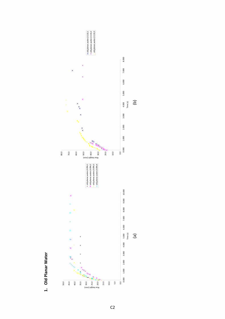
1. Old Plana

r Water 

   

0.0

5.0

10.0

15.0

20.0

25.0

30.0

35.0

40.0

45.0

50.0 0.

000

1.000

2.000

3.000

4.000

5.000

6.000

7.000

8.000

9.000

10.000

Time (s)

Rise Height (mm)

old,planar,water,0.094,1

old,planar,water,0.094,2

old,planar,water,0.094,3

old,planar,water,0.094,4

0.0

10.0

20.0

30.0

40.0

50.0

60.0

70.0

80.0 0.

000

1.000

2.000

3.000

4.000

5.000

6.000

7.000

8.000

Time (s)

Rise Height (mm)

old,planar,water,0.110,1

old,planar,water,0.110,2

old,planar,water,0.110,3

  

  

            (a) 

  

  

  

  

         (b) 

C2

0.0

10.0

20.0

30.0

40.0

50.0

60.0

70.0 0.

000

1.000

2.000

3.000

4.000

5.000

6.000

7.000

8.000

Time (s)

Rise Height (mm)

old,planar,water,0.237,1

old,planar,water,0.237,2

old,planar,water,0.237,3

old,planar,water,0.237,4

0.0

10.0

20.0

30.0

40.0

50.0

60.0 0.

000

1.000

2.000

3.000

4.000

5.000

6.000

7.000

8.000

Time (s)

Rise Height (mm)

old,planar,water,0.254,1

old,planar,water,0.254,2

old,planar,water,0.254,3

                                                     (c) 

  

  

  

  

     (d)       

0.0

10.0

20.0

30.0

40.0

50.0

60.0

70.0 0.

000

1.000

2.000

3.000

4.000

5.000

6.000

7.000

8.000

Time (s)

Rise Height (mm)

old,planar,water,0.261,1

old,planar,water,0.261,2

0.0

5.0

10.0

15.0

20.0

25.0

30.0

35.0

40.0

45.0

50.0 0.

000

1.000

2.000

3.000

4.000

5.000

6.000

7.000

8.000

Time (s)

Rise Height (mm)

old,planar,water,0.344,1

old,planar,water,0.344,2

old,planar,water,0.344,3

  (e)

(f) 

  

C3

0.0

5.0

10.0

15.0

20.0

25.0

30.0

35.0

40.0 0.

000

1.000

2.000

3.000

4.000

5.000

6.000

7.000

8.000

Time (s)

Rise Height (mm)

old,planar,water,0.502,1

old,planar,water,0.502,2

old,planar,water,0.502,3

 

0.0

5.0

10.0

15.0

20.0

25.0

30.0

35.0 0.

000

1.000

2.000

3.000

4.000

5.000

6.000

7.000

8.000

Time (s)

Rise Height (mm)

old,planar,water,0.620,1

old,planar,water,0.620,2

old,planar,water,0.620,3

                                                    (g)                                                    

  

           

        (h)  

0.0

5.0

10.0

15.0

20.0

25.0

30.0 0.

000

1.000

2.000

3.000

4.000

5.000

6.000

7.000

8.000

Time (s)

Rise Height (mm)

old,planar,water,0.714,1

old,planar,water,0.714,2

old,planar,water,0.714,3

0.0

2.0

4.0

6.0

8.0

10.0

12.0 0.

000

1.000

2.000

3.000

4.000

5.000

6.000

7.000

8.000

Time (s)

Rise Height (mm)

old,planar,water,0.900

 (i)

(j) 

 

C4

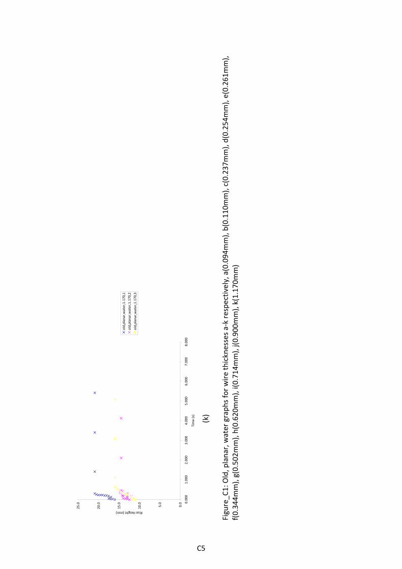
0.0

5.0

10.0

15.0

20.0

25.0 0.

000

1.000

2.000

3.000

4.000

5.000

6.000

7.000

8.000

Time (s)

Rise Height (mm)

old,planar,water,1.170,1

old,planar,water,1.170,2

old,planar,water,1.170,3

  

 (k)                                                                                                                         

  Figure_C

1: Old, planar, water graph

s for wire thicknesses a‐k respectively, a(0.094mm), b(0.11

0mm), c(0.237m

m), d(0.25

4mm), e(0.26

1mm), 

f(0.34

4mm), g(0.50

2mm), h(0.620m

m), i(0

.714

mm), j(0

.900mm), k(1.170m

m) 

                       

C5

2. Old Tap

ered

 Water 

 

0.0

10.0

20.0

30.0

40.0

50.0

60.0

70.0 0.

000

1.000

2.000

3.000

4.000

5.000

6.000

7.000

8.000

9.000

10.000

Time (s)

Rise Height (mm)

old,tape

red,water,0.094

‐0.110,1

old,tape

red,water,0.094

‐0.110,2

0.0

10.0

20.0

30.0

40.0

50.0

60.0

70.0 0.

000

1.000

2.000

3.000

4.000

5.000

6.000

7.000

8.000

9.000

10.000

Time (s)

Rise Height (mm)

old,tape

red,water,0.110

‐0.261,1

old,tape

red,water,0.110

‐0.261,2

old,tape

red,water,0.110

‐0.261,3

      

        (a)               

  

  

  

              (b) 

 

C6

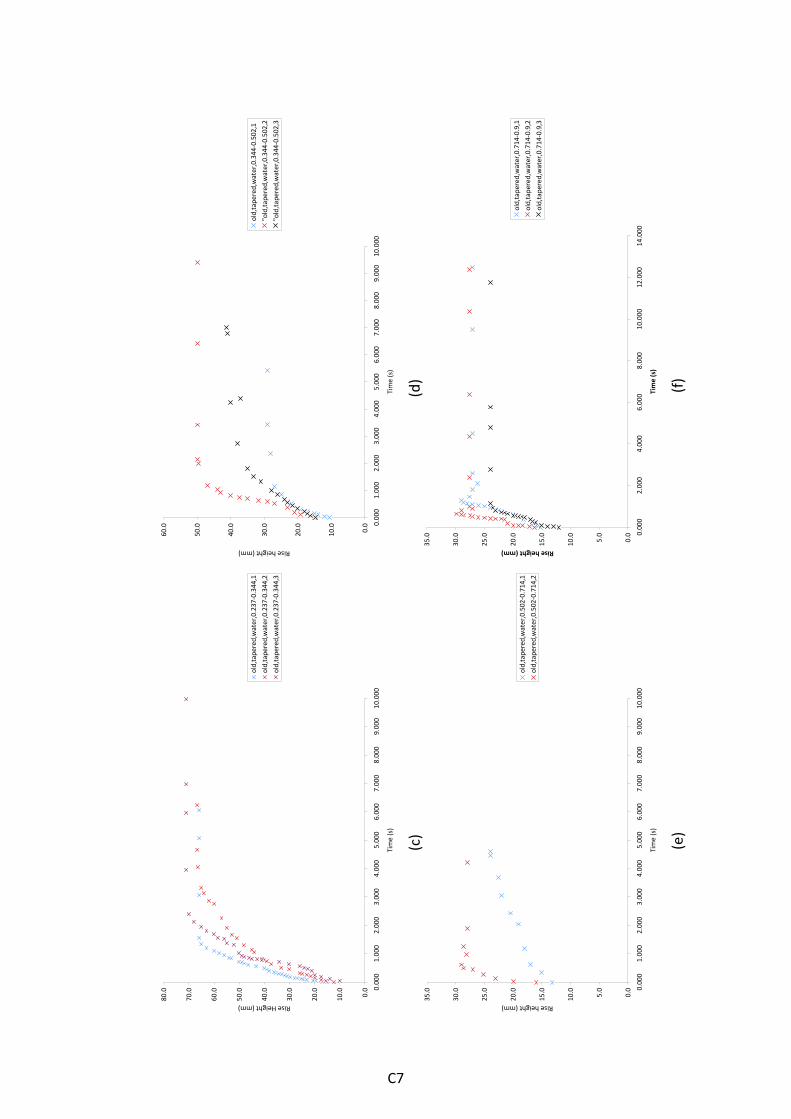
0.0

10.0

20.0

30.0

40.0

50.0

60.0

70.0

80.0 0.

000

1.000

2.000

3.000

4.000

5.000

6.000

7.000

8.000

9.000

10.000

Time (s)

Rise Height (mm)

old,tape

red,water,0.237

‐0.344,1

old,tape

red,water,0.237

‐0.344,2

old,tape

red,water,0.237

‐0.344,3

0.0

10.0

20.0

30.0

40.0

50.0

60.0 0.

000

1.000

2.000

3.000

4.000

5.000

6.000

7.000

8.000

9.000

10.000

Time (s)

Rise height (mm)

old,tape

red,water,0.344

‐0.502,1

"old,tapered

,water,0.344

‐0.502,2

"old,tapered

,water,0.344

‐0.502,3

  

  

        (c)  

  

  

  

  

 (d) 

0.0

5.0

10.0

15.0

20.0

25.0

30.0

35.0 0.

000

1.000

2.000

3.000

4.000

5.000

6.000

7.000

8.000

9.000

10.000

Time (s)

Rise height (mm)

old,tape

red,water,0.502

‐0.714,1

old,tape

red,water,0.502

‐0.714,2

0.0

5.0

10.0

15.0

20.0

25.0

30.0

35.0 0.

000

2.000

4.000

6.000

8.000

10.000

12.000

14.000

Time (s)

Rise height (mm)

old,tape

red,water,0.714

‐0.9,1

old,tape

red,water,0.714

‐0.9,2

old,tape

red,water,0.714

‐0.9,3

 (e)

(f) 

 

C7

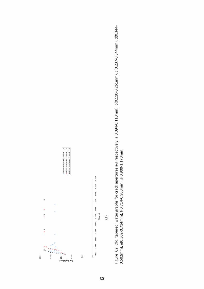
0.0

5.0

10.0

15.0

20.0

25.0 0.

000

1.000

2.000

3.000

4.000

5.000

6.000

7.000

8.000

9.000

10.000

Time (s)

Rise Height (mm)

old,tape

red,water,0.900

‐1.17,1

old,tape

red,water,0.900

‐1.17,2

old,tape

red,water,0.900

‐1.17,3

  

  

        (g) 

  Figure_C

2: Old, tapered

, water graph

s for crack apertures a‐g respectiv

ely, a(0.094

‐0.110

mm), b(0.110‐0.26

1mm), c(0.237‐0.34

4mm), d(0.344‐

0.50

2mm), e(0.502‐0.71

4mm), f(0.714‐0.900m

m), g(0.900‐1.17

0mm) 

                       

C8

3. Old Tortuou

s 3 an

d 5 Nod

es W

ater  

 

0.00

5.00

10.00

15.00

20.00

25.00

30.00

35.00

40.00

45.00 0.

002.00

4.00

6.00

8.00

10.00

12.00

14.00

Time (s)

Rise height (mm)

Old, Tortuou

s, 3 nod

es, W

ater, 0.094, 1

Old, Tortuou

s, 3 nod

es, W

ater, 0.094, 2

Old, Tortuou

s, 3 nod

es, W

ater, 0.094, 3

0.00

10.00

20.00

30.00

40.00

50.00

60.00 0.

002.00

4.00

6.00

8.00

10.00

12.00

Time (s)

Rise height (mm)

Old, Tortuou

s, 3 nod

es, W

ater, 0.170, 1

Old, Tortuou

s, 3 nod

es, W

ater, 0.170, 2

Old, Tortuou

s, 3 nod

es, W

ater, 0.170, 3

 (a)

(b) 

 

C9

 

0.00

10.00

20.00

30.00

40.00

50.00

60.00

70.00 0.

002.00

4.00

6.00

8.00

10.00

12.00

14.00

Time (s)

Rise height (mm)

Old, Tortuou

s, 3 nod

es, W

ater, 0.254, 1

Old, Tortuou

s, 3 nod

es, W

ater, 0.254, 2 

Old, Tortuou

s, 3 nod

es, W

ater, 0.254, 3

 

0.00

10.00

20.00

30.00

40.00

50.00

60.00

70.00 0.

002.00

4.00

6.00

8.00

10.00

12.00

14.00

Time(s)

Rise height (mm)

Old, Tortuou

s, 3 nod

es, W

ater, 0.344, 1

Old, Tortuou

s, 3 nod

es, W

ater, 0.344, 2

   

  

      (c)   

  

  

  

  

 (d) 

0.00

5.00

10.00

15.00

20.00

25.00

30.00 0.

001.00

2.00

3.00

4.00

5.00

6.00

7.00

8.00

9.00

Time (s)

Rise height (mm)

Old, Tortuou

s, 3 nod

es, W

ater, 0.502, 1

Old, Tortuou

s, 3 nod

es, W

ater, 0.502, 2 

Old, Tortuou

s, 3 nod

es, W

ater, 0.502, 3

0.00

5.00

10.00

15.00

20.00

25.00 0.

001.00

2.00

3.00

4.00

5.00

6.00

7.00

8.00

9.00

Time (s)

Rise height (mm)

Old, Tortuou

s, 3 nod

es, W

ater, 0.714, 1

Old, Tortuou

s, 3 nod

es, W

ater, 0.714, 2

Old, Tortuou

s, 3 nod

es, W

ater, 0.714, 3

 (e)

(f) 

  

C10

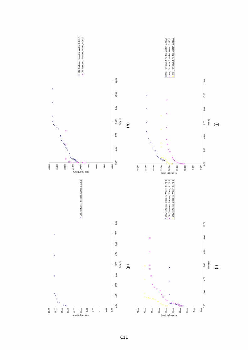
0.00

2.00

4.00

6.00

8.00

10.00

12.00

14.00

16.00

18.00

20.00 0.

001.00

2.00

3.00

4.00

5.00

6.00

7.00

8.00

Time (s)

Rise height (mm)

Old, Tortuou

s, 3 nod

es, W

ater, 0.900,1

 

0.00

5.00

10.00

15.00

20.00

25.00

30.00

35.00

40.00 0.

002.00

4.00

6.00

8.00

10.00

12.00

Time (s)

Rise height (mm)

Old, Tortuou

s, 5 nod

es, W

ater, 0.094, 1

Old, Tortuou

s, 5 Nod

es, W

ater, 0.094,2

   

  

     (g)  

  

  

  

            (h) 

 

0.00

5.00

10.00

15.00

20.00

25.00

30.00

35.00

40.00

45.00 0.

002.00

4.00

6.00

8.00

10.00

12.00

Time (s)

Rise height (mm)

Old, Tortuou

s, 5 Nod

es, W

ater, 0.170, 1

Old, Tortuou

s, 5 Nod

es, W

ater, 0.170, 2

Old, Tortuou

s, 5 Nod

es, W

ater, 0.170, 3

0.00

5.00

10.00

15.00

20.00

25.00

30.00

35.00

40.00 0.

002.00

4.00

6.00

8.00

10.00

12.00

Time (s)

Rise height (mm)

Old, Tortuou

s, 5 Nod

es, W

ater, 0.280, 1

Old, Tortuou

s, 5 Nod

es, W

ater, 0.280, 2

Old, Tortuou

s, 5 Nod

es, W

ater, 0.280, 3

  (i)

(j) 

 

C11

  

 

0.00

5.00

10.00

15.00

20.00

25.00

30.00

35.00

40.00 0.

002.00

4.00

6.00

8.00

10.00

12.00

14.00

Time (s)

Rise height (mm)

Old, Tortuou

s, 5 Nod

es, W

ater, 0.344, 1

Old, Tortuou

s, 5 Nod

es, W

ater, 0.344, 2

Old, Tortuou

s, 5 Nod

es, W

ater, 0.344, 3

 

0.00

5.00

10.00

15.00

20.00

25.00

30.00

35.00 0.

001.00

2.00

3.00

4.00

5.00

6.00

7.00

Time (s)

Rise height (mm)

Old, Tortuou

s, 5 Nod

es, W

ater, 0.502, 1

Old, Tortuou

s, 5 Nod

es, W

ater, 0.502, 2

Old, Tortuou

s, 5 Nod

es, W

ater, 0.502, 3

  

  

     (k)  

  

  

  

  

(l) 

        

  

    

C12

 

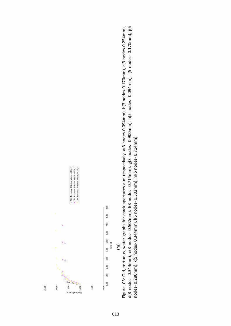
0.00

5.00

10.00

15.00

20.00

25.00 0.

001.00

2.00

3.00

4.00

5.00

6.00

7.00

8.00

9.00

Time (s)

Rise height (mm)

Old, Tortuou

s, 5 Nod

es, W

ater, 0.714, 1

Old, Tortuou

s, 5 Nod

es, W

ater, 0.714, 2

Old, Tortuou

s, 5 Nod

es, W

ater, 0.714, 3

  

  

      (m

) Figure_C

3: Old, tortuou

s, water graph

s for crack apertures a‐m respe

ctively, a(3 nod

es‐0.094mm), b(3 no

des‐0.17

0mm), c(3 no

des‐0.25

4mm),  

d(3 no

des‐ 0.344

mm), e(3 no

des‐ 0.502

mm), f(3 no

des‐ 0.714

mm), g(3 no

des‐ 0.900

mm), h(5 no

des‐ 0.094

mm), i(5

 nod

es‐ 0.17

0mm), j(5

 no

des‐ 0.280

mm), k(5 no

des‐ 0.344

mm), l(5

 nod

es‐ 0

.502mm), m(5 nod

es‐ 0

.714mm) 

                       

C13

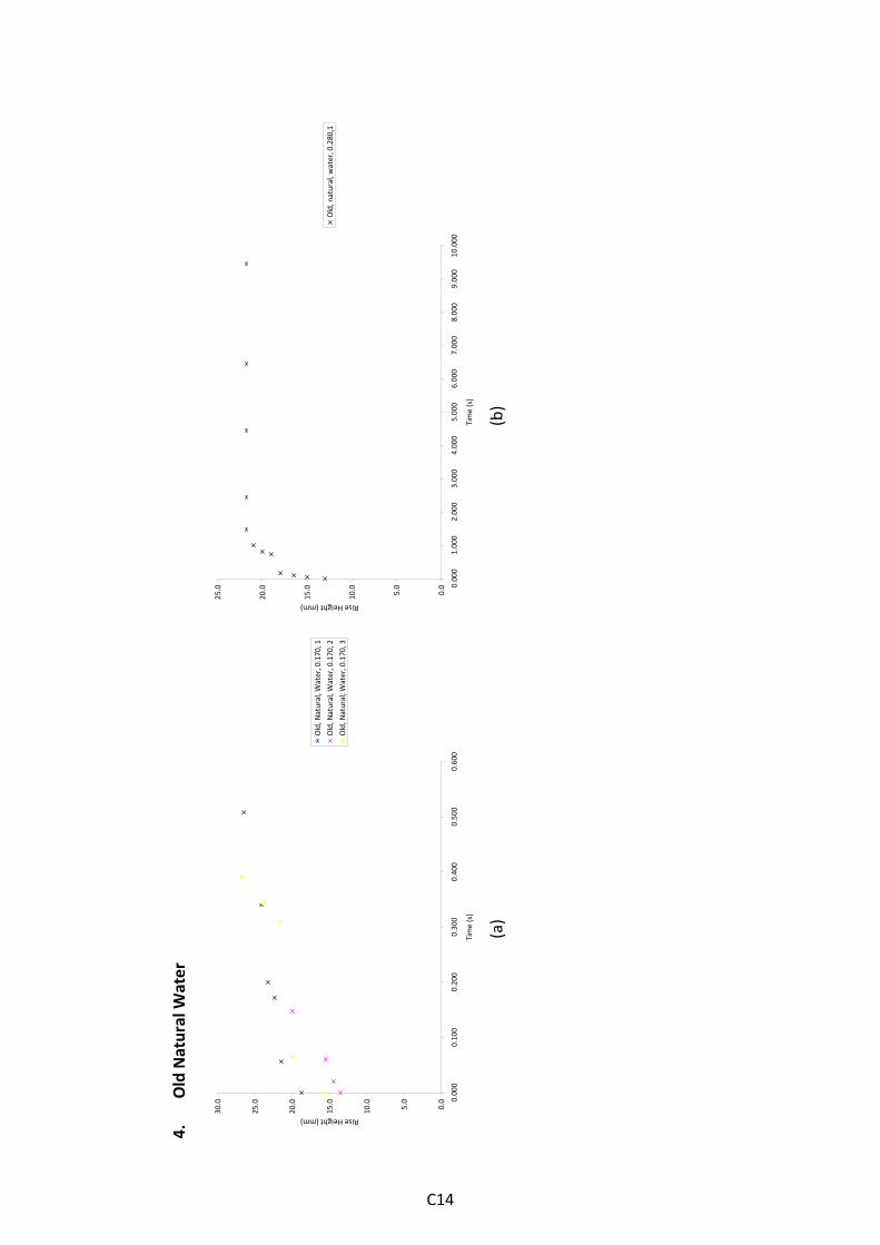
4.

Old Natural W

ater 

 

0.0

5.0

10.0

15.0

20.0

25.0

30.0 0.

000

0.100

0.200

0.300

0.400

0.500

0.600

Time (s)

Rise Height (mm)

Old, N

atural, W

ater, 0.170, 1

Old, N

atural, W

ater, 0.170, 2

Old, N

atural, W

ater, 0.170, 3

  

0.0

5.0

10.0

15.0

20.0

25.0 0.

000

1.000

2.000

3.000

4.000

5.000

6.000

7.000

8.000

9.000

10.000

Time (s)

Rise Height (mm)

Old, natural, w

ater, 0.280,1

   

  

          (a) 

  

  

  

  

     (b) 

 

C14

0.0

5.0

10.0

15.0

20.0

25.0 0.

000

1.000

2.000

3.000

4.000

5.000

6.000

7.000

8.000

9.000

Time (s)

Rise Height (mm)

Old, natural, w

ater, 0.344,1

 

0.0

5.0

10.0

15.0

20.0

25.0 0.

000

1.000

2.000

3.000

4.000

5.000

6.000

7.000

8.000

9.000

10.000

Time (s)

Rise Height (mm)

Old, natural, w

ater, 0.502,1

  

  

          (c)  

  

  

  

  

     (d) 

       

C15

0.0

5.0

10.0

15.0

20.0

25.0 0.

000

1.000

2.000

3.000

4.000

5.000

6.000

7.000

8.000

9.000

Time (s)

Rise Height (mm)

Old, natural, w

ater, 0.620, 1

Old, natural, w

ater, 0.620, 2

Old, natural, w

ater, 0.620, 3

 

11.5

12.0

12.5

13.0

13.5

14.0

14.5 0.

000

2.000

4.000

6.000

8.000

10.000

12.000

Time (s)

Rise Height (mm)

Old, natural, w

ater, 0.714,1

  

  

          (e

)  

  

  

  

      (f) 

  Figure_C

4: Old, natural, w

ater graph

s for crack apertures a‐f respe

ctively, a(0.170mm), b(0.28

0mm), c(0.344m

m), d(0.50

2mm), e(0.62

0mm), 

f(0.71

4mm) 

                       

C16

5. Old Plana

r Cyan

oacrylate 

 

0.0

5.0

10.0

15.0

20.0

25.0

30.0

35.0

40.0 0.

000

1.000

2.000

3.000

4.000

5.000

6.000

7.000

8.000

Time/s

Rise Height/mm

Old, planar, cyano

acrylate, 0.110, 1

Old, planar, cyano

acrylate, 0.110, 2

 

0.0

5.0

10.0

15.0

20.0

25.0

30.0

35.0 0.

000

1.000

2.000

3.000

4.000

5.000

6.000

7.000

8.000

Time/s

Rise height/mm

Old, planar, cyano

acrylate, 0.261, 1

Old, planar, cyano

acrylate, 0.261, 2

Old, planar, cyano

acrylate, 0.261, 3

  

  

       (a)  

  

  

  

  

  (b) 

  

C17

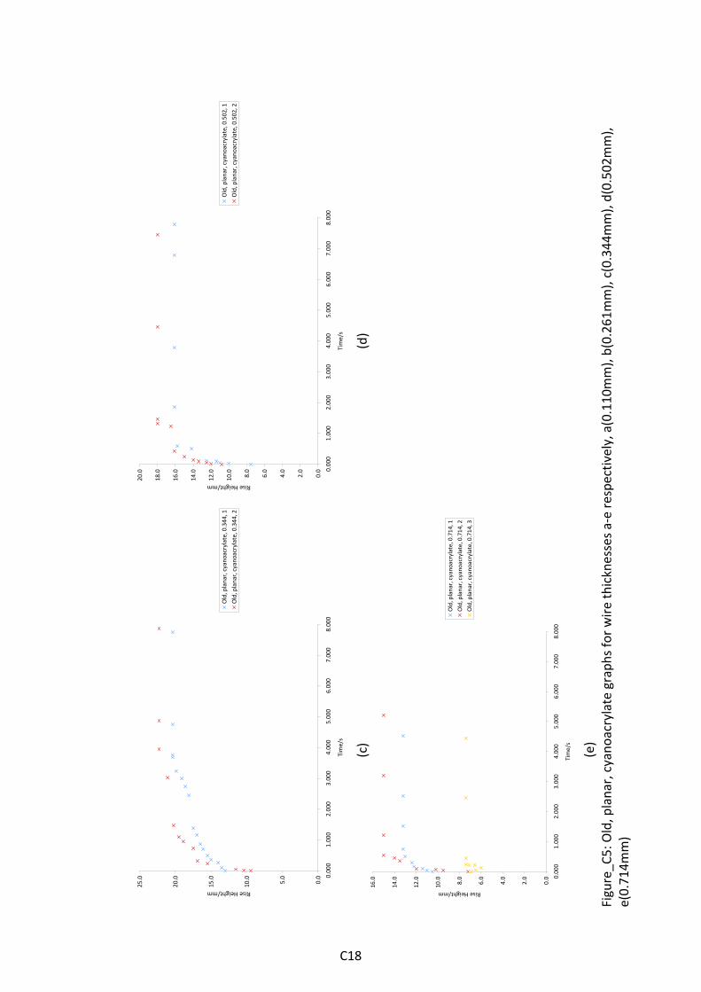
0.0

5.0

10.0

15.0

20.0

25.0 0.

000

1.000

2.000

3.000

4.000

5.000

6.000

7.000

8.000

Time/s

Rise Height/mm

Old, planar, cyano

acrylate, 0.344, 1

Old, planar, cyano

acrylate, 0.344, 2

 

0.0

2.0

4.0

6.0

8.0

10.0

12.0

14.0

16.0

18.0

20.0 0.

000

1.000

2.000

3.000

4.000

5.000

6.000

7.000

8.000

Time/s

Rise Height/mm

Old, planar, cyano

acrylate, 0.502, 1

Old, planar, cyano

acrylate, 0.502, 2

   

  

       (c)   

  

  

  

  

  (d) 

0.0

2.0

4.0

6.0

8.0

10.0

12.0

14.0

16.0 0.

000

1.000

2.000

3.000

4.000

5.000

6.000

7.000

8.000

Time/s

Rise Height/mm

Old, planar, cyano

acrylate, 0.714, 1

Old, planar, cyano

acrylate, 0.714, 2

Old, planar, cyano

acrylate, 0.714, 3

  

  

       (e

) Figure_C

5: Old, planar, cyano

acrylate graph

s for wire thicknesses a‐e respectiv

ely, a(0.110mm), b(0.26

1mm), c(0.344m

m), d(0.502m

m), 

e(0.714m

m) 

C18

6. Old Tap

ered

 Cyano

acrylate 

 

0.0

10.0

20.0

30.0

40.0

50.0

60.0 0.

000

1.000

2.000

3.000

4.000

5.000

6.000

7.000

8.000

Time/s

Rise Height/mm

Old, Tapered

, Cyano

acrylate, 0.094

‐0.110, 1

Old, Tapered

, Cyano

acrylate, 0.094

‐0.110, 2

Old, Tapered

, Cyano

acrylate, 0.094

‐0.110, 3

  

0.0

5.0

10.0

15.0

20.0

25.0

30.0

35.0

40.0

45.0 0.

000

1.000

2.000

3.000

4.000

5.000

6.000

7.000

8.000

Time/s

Rise Height/mm

Old, Tapered

, Cyano

acrylate, 0.110

‐0.254, 1

Old, Tapered

, Cyano

acrylate, 0.110

‐0.254, 2

  (a)

(b) 

   

C19

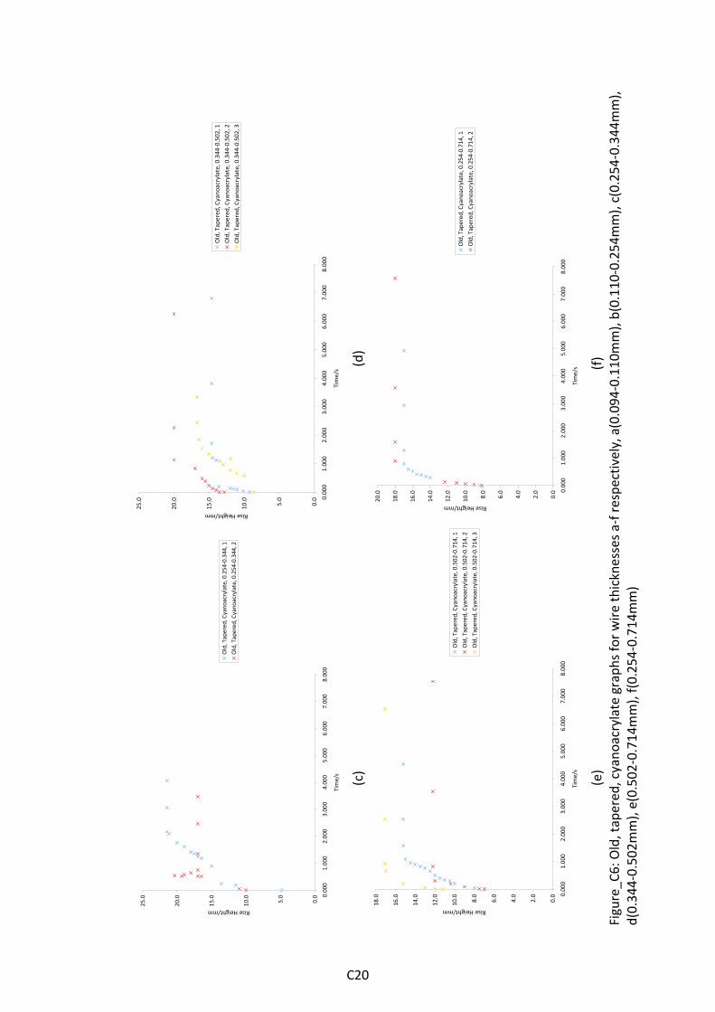
0.0

5.0

10.0

15.0

20.0

25.0 0.

000

1.000

2.000

3.000

4.000

5.000

6.000

7.000

8.000

Time/s

Rise Height/mm

Old, Tapered

, Cyano

acrylate, 0.254

‐0.344, 1

Old, Tapered

, Cyano

acrylate, 0.254

‐0.344, 2

  

0.0

5.0

10.0

15.0

20.0

25.0 0.

000

1.000

2.000

3.000

4.000

5.000

6.000

7.000

8.000

Time/s

Rise Height/mm

Old, Tapered

, Cyano

acrylate, 0.344

‐0.502, 1

Old, Tapered

, Cyano

acrylate, 0.344

‐0.502, 2

Old, Tapered

, Cyano

acrylate, 0.344

‐0.502, 3

   

  

   (c)  

  

  

  

  

            (d) 

0.0

2.0

4.0

6.0

8.0

10.0

12.0

14.0

16.0

18.0 0.

000

1.000

2.000

3.000

4.000

5.000

6.000

7.000

8.000

Time/s

Rise Height/mm

Old, Tapered, Cyano

acrylate, 0.502

‐0.714, 1

Old, Tapered, Cyano

acrylate, 0.502

‐0.714, 2

Old, Tapered, Cyano

acrylate, 0.502

‐0.714, 3 

 

0.0

2.0

4.0

6.0

8.0

10.0

12.0

14.0

16.0

18.0

20.0 0.

000

1.000

2.000

3.000

4.000

5.000

6.000

7.000

8.000

Time/s

Rise Height/mm

Old, Tapered

, Cyano

acrylate, 0.254

‐0.714, 1 

Old, Tapered

, Cyano

acrylate, 0.254

‐0.714, 2

  

  

   (e) 

  

  

  

  

           (f) 

Figure_C

6: Old, tapered

, cyano

acrylate graph

s for wire thicknesses a‐f respe

ctively, a(0.094

‐0.110

mm), b(0.110‐0.25

4mm), c(0.254‐0.34

4mm), 

d(0.344‐0.50

2mm), e(0.502‐0.714m

m), f(0.254‐0.71

4mm) 

C20

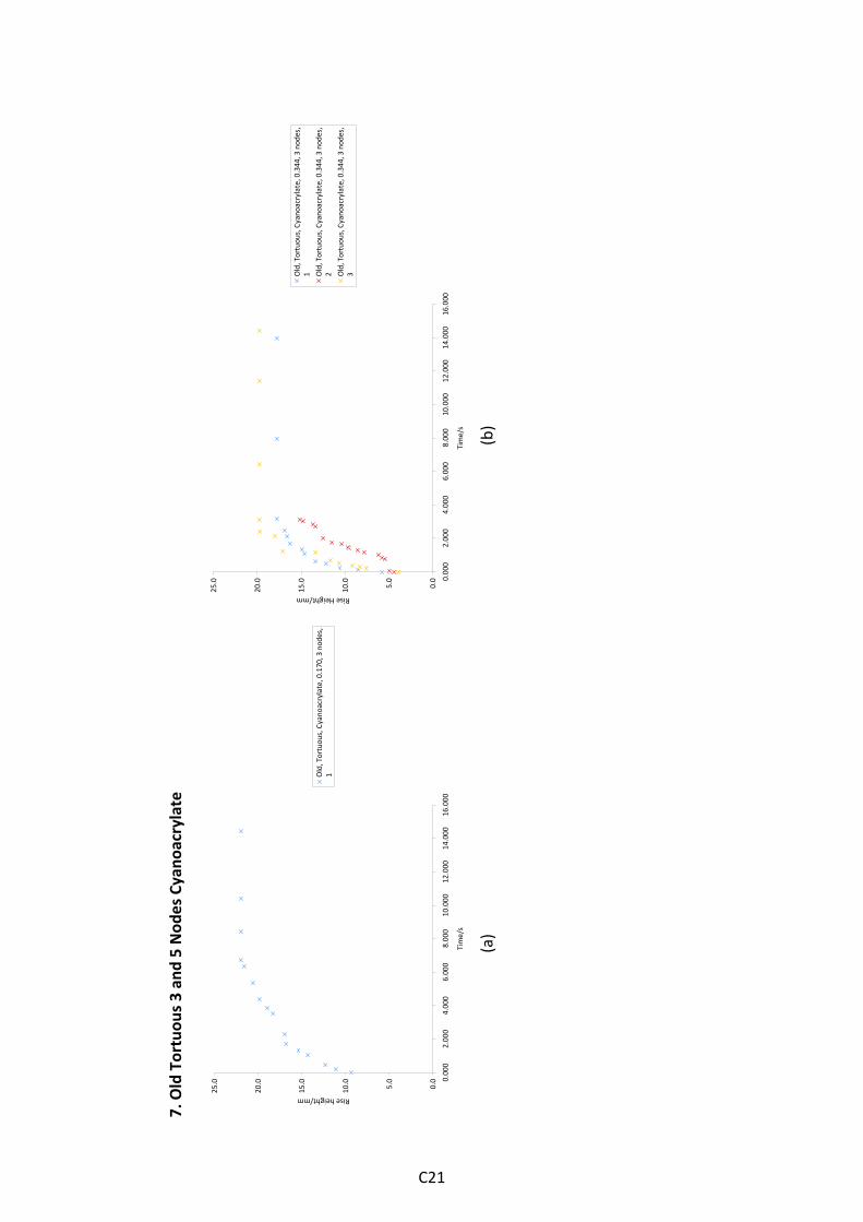
7. Old Tortuou

s 3 an

d 5 Nod

es Cyano

acrylate 

 

0.0

5.0

10.0

15.0

20.0

25.0 0.

000

2.000

4.000

6.000

8.000

10.000

12.000

14.000

16.000

Time/s

Rise height/mm

Old, Tortuou

s, Cyano

acrylate, 0.170, 3 nod

es,

1

 

0.0

5.0

10.0

15.0

20.0

25.0 0.

000

2.000

4.000

6.000

8.000

10.000

12.000

14.000

16.000

Time/s

Rise Height/mm

Old, Tortuou

s, Cyano

acrylate, 0.344, 3 nod

es,

1 Old, Tortuou

s, Cyano

acrylate, 0.344, 3 nod

es,

2 Old, Tortuou

s, Cyano

acrylate, 0.344, 3 nod

es,

3

 (a)

(b)  

 

C21

0.0

2.0

4.0

6.0

8.0

10.0

12.0

14.0

16.0 0.

000

2.000

4.000

6.000

8.000

10.000

12.000

14.000

16.000

Time/s

Rise Height/mm

Old, Tortuou

s, Cyano

acrylate, 3 Nod

es, 0.502,

1 Old, Tortuou

s, Cyano

acrylate, 3 Nod

es, 0.502,

2  Old, Tortuou

s, Cyano

acrylate, 3 Nod

es, 0.502,

3

 

0.0

1.0

2.0

3.0

4.0

5.0

6.0

7.0

8.0

9.0

10.0 0.

000

1.000

2.000

3.000

4.000

5.000

Time/s

Rise Height/mm

Old, Tortuou

s, Cyano

acrylate, 3 Nod

es, 0.714,

1 Old, Tortuou

s, Cyano

acrylate, 3 Nod

es, 0.714,

2

  

  

  (c)  

  

  

  

  

          (d

)  

0.0

2.0

4.0

6.0

8.0

10.0

12.0

14.0 0.

000

2.000

4.000

6.000

8.000

10.000

12.000

14.000

16.000

Time/s

Rise Height/mm

Old, Tortuou

s, Cyano

acrylate, 5 nod

es, 0.094,

1 Old, Tortuou

s, Cyano

acrylate, 5 nod

es, 0.094,

2

 

0.0

2.0

4.0

6.0

8.0

10.0

12.0

14.0

16.0

18.0 0.

000

1.000

2.000

3.000

4.000

5.000

6.000

7.000

8.000

Time/s

Rise Height/mm

Old, Tortuou

s, Cyano

acrylate, 5 nod

es, 0.170,

1 Old, Tortuou

s, Cyano

acrylate, 5 nod

es, 0.170,

2 Old, Tortuou

s, Cyano

acrylate, 5 nod

es, 0.170,

3

  

  

  (e) 

  

  

  

  

           (f)  

C22

0.0

2.0

4.0

6.0

8.0

10.0

12.0

14.0

16.0

18.0

20.0 0.

000

1.000

2.000

3.000

4.000

5.000

6.000

7.000

8.000

Time/s

Rise Height/mm

Old, Tortuou

s, Cyano

acrylate, 5 nod

es, 0.344,

1 Old, Tortuou

s, Cyano

acrylate, 5 nod

es, 0.344,

2

 

0.0

2.0

4.0

6.0

8.0

10.0

12.0 0.

000

0.500

1.000

1.500

2.000

2.500

3.000

3.500

4.000

Time/s

Rise Height/mm

Old, Tortuou

s, Cyano

acrylate, 5 nod

es, 0.502,

1 Old, Tortuou

s, Cyano

acrylate, 5 nod

es, 0.502,

2 Old, Tortuou

s, Cyano

acrylate, 5 nod

es, 0.502,

3

   

  

   (g) 

  

  

  

  

          (h

) 

0.0

1.0

2.0

3.0

4.0

5.0

6.0

7.0

8.0 0.000

0.200

0.400

0.600

0.800

1.000

1.200

Time/s

Rise Height/mm

Old, Tortuou

s, Cyano

acrylate, 5 nod

es, 0.714,

1 Old, Tortuou

s, Cyano

acrylate, 5 nod

es, 0.714,

2

  

  

(i) 

Figure_C

7: Old Tortuou

s 3 and 5 Nod

es Cyano

acrylate water graph

s for wire thicknesses a‐i respe

ctively, a(3 nod

es, 0.170

mm), b(3 no

des, 

0.34

4mm), c(3 no

des, 0.502

mm), d(3 no

des, 0.714

mm), e(5 no

des, 0.094

mm), f(5 no

des, 0.170

mm), g(5 no

des, 0.344mm), h(5 no

des, 

0.50

2mm), i(5

 nod

es, 0.714

mm) 

C23

8. You

ng Plana

r Water 

 

0.0

10.0

20.0

30.0

40.0

50.0

60.0

70.0

80.0 0.

000

5.000

10.000

15.000

20.000

25.000

Time/s

Rise Height/mm

Youn

g, planar, water, 0.094, 1

 

0.0

5.0

10.0

15.0

20.0

25.0

30.0

35.0

40.0

45.0

50.0 0.

000

2.000

4.000

6.000

8.000

10.000

12.000

Time/s

Rise Height/mm

Youn

g, planar, cyano

acrylate, 0.110, 1

  (a)

(b) 

 

C24

0.0

5.0

10.0

15.0

20.0

25.0

30.0

35.0

40.0

45.0 0.

000

2.000

4.000

6.000

8.000

10.000

12.000

14.000

Time/s

Rise Height/mm

Youn

g, planar, water, 0.344, 1

Youn

g, planar, water, 0.344, 2

Youn

g, planar, water, 0.344, 3

 

0.0

5.0

10.0

15.0

20.0

25.0

30.0

35.0

40.0

45.0

50.0 0.

000

2.000

4.000

6.000

8.000

10.000

12.000

14.000

16.000

Time/s

Rise Height/mm

youn

g, planar, water, 0.502, 1

youn

g, planar, water, 0.502, 2

youn

g, planar, water, 0.502, 3

   

          (c) 

  

  

  

  

    (d

) 

0.0

5.0

10.0

15.0

20.0

25.0

30.0 0.

000

2.000

4.000

6.000

8.000

10.000

12.000

14.000

Time/s

Rise Height/mm

Youn

g, planar, water, 0.714, 1

Youn

g, planar, water, 0.714, 2

Youn

g, planar, water, 0.714, 3

 

0.0

5.0

10.0

15.0

20.0

25.0

30.0 0.

000

2.000

4.000

6.000

8.000

10.000

12.000

14.000

Time/s

Rise Height/mm

youn

g, planar, water, 0.900, 1

youn

g, planar, water, 0.900, 2

youn

g, planar, water, 0.900, 3

  

  

        (e)  

  

  

  

  

   (f) 

Figure_C

8: You

ng planar water graph

s for wire thicknesses a‐f respe

ctively, a(0.094mm), b(0.11

0mm), c(0.344m

m), d(0.50

2mm), e(0.71

4mm), 

f(0.90

0mm) 

C25

9. You

ng Tap

ered

 Water 

 

0.0

10.0

20.0

30.0

40.0

50.0

60.0

70.0

80.0 0.

000

1.000

2.000

3.000

4.000

5.000

6.000

7.000

8.000

Time/s

Rise Height/mm

Youn

g, ta

pered, water, 0.094

‐0.170, 1

 

010203040506070

0.000

1.000

2.000

3.000

4.000

5.000

6.000

7.000

8.000

Time/s

Rise Height/mm

Youn

g, ta

pered, water, 0.170

‐0.280

  

  

      (a)  

  

  

  

  

 (b) 

  

0510152025303540

0.000

1.000

2.000

3.000

4.000

5.000

6.000

Time/s

Rise Height/mm

Youn

g, ta

pered, water, 0.280

‐0.502,1

 

18

18.519

19.520

20.521

21.522

22.5 0.

000

1.000

2.000

3.000

4.000

5.000

6.000

7.000

8.000

Time/s

Rise Height/mm

Youn

g, ta

pered, water, 0.502

‐0.714,1

   

  

     (c)  

  

  

  

  

 (d) 

C26

012345678 0.000

1.000

2.000

3.000

4.000

5.000

6.000

Time/s

Rise Height/mm

Youn

g, ta

pered, water, 0.714

‐0.9,1

 

05101520253035

0.000

0.500

1.000

1.500

2.000

2.500

3.000

3.500

4.000

Time/s

Rise Height/mm

Youn

g, ta

pered, water, 0.094

‐0.502

 (e)

(f) 

 Figure_C

9: You

ng, tapered

, water graph

s for wire thicknesses a‐k respectively, a(0.094

‐0.170

mm), b(0.170‐0.28

0mm), c(0.34

4‐0.50

2mm), 

d(0.502‐0.71

4mm), e(0.714‐0.900m

m), f(0.094‐0.50

2mm) 

                       

C27

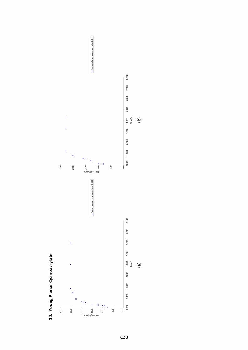
10.  Yo

ung Plan

ar Cyano

acrylate 

 

0.0

5.0

10.0

15.0

20.0

25.0

30.0 0.

000

1.000

2.000

3.000

4.000

5.000

6.000

7.000

8.000

Time/s

Rise Height/mm

Youn

g, planar, cyano

acrylate, 0.261

 

0.0

5.0

10.0

15.0

20.0

25.0 0.

000

1.000

2.000

3.000

4.000

5.000

6.000

7.000

8.000

Time/s

Rise Height/mm

Youn

g, planar, cyano

acrylate, 0.344

  (a)

(b) 

 

C28

0.0

1.0

2.0

3.0

4.0

5.0

6.0

7.0 0.000

1.000

2.000

3.000

4.000

5.000

6.000

7.000

8.000

Time/s

Rise Height/mm

Youn

g, planar, cyano

acrylate, 0.502

 

0.0

2.0

4.0

6.0

8.0

10.0

12.0

14.0 0.

000

1.000

2.000

3.000

4.000

5.000

6.000

7.000

8.000

Time/s

Rise Height/mm

Youn

g, planar, cyano

acrylate, 0.714

  

  

       (c)  

  

  

  

  

  (d) 

  

  

Figure_C

10: You

ng planar cyanoacrylate graphs fo

r wire thicknesses a‐d respectiv

ely, a(0.261mm), b(0.344m

m), c(0.50

2mm), d(0.71

4mm) 

                         

C29

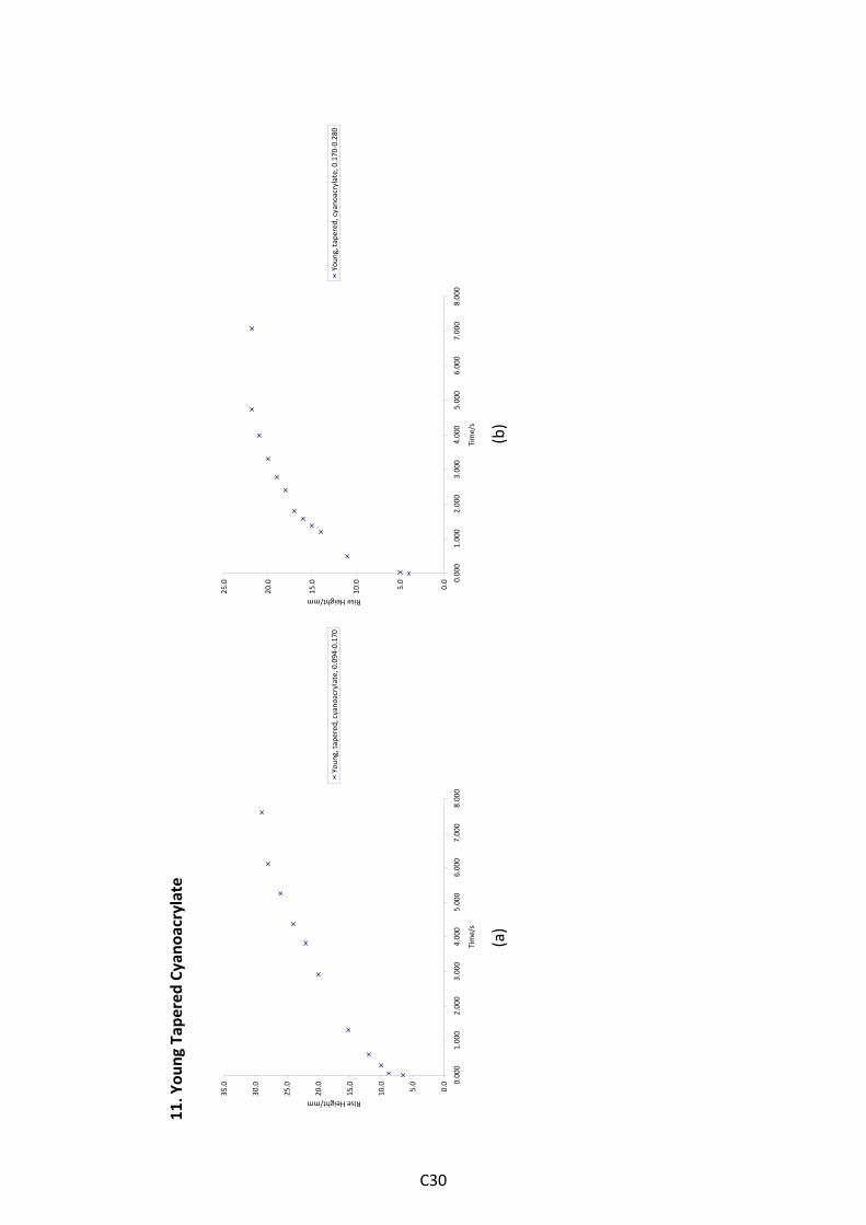
11. You

ng Tap

ered

 Cyano

acrylate 

 

0.0

5.0

10.0

15.0

20.0

25.0

30.0

35.0 0.

000

1.000

2.000

3.000

4.000

5.000

6.000

7.000

8.000

Time/s

Rise Height/mm

Youn

g, ta

pered, cyano

acrylate, 0.094

‐0.170

 

0.0

5.0

10.0

15.0

20.0

25.0 0.

000

1.000

2.000

3.000

4.000

5.000

6.000

7.000

8.000

Time/s

Rise Height/mm

Youn

g, ta

pered, cyano

acrylate, 0.170

‐0.280

  

  

    (a) 

  

  

  

  

            (b)  

 

C30

0.0

2.0

4.0

6.0

8.0

10.0

12.0

14.0

16.0

18.0

20.0 0.

000

1.000

2.000

3.000

4.000

5.000

6.000

7.000

8.000

Time/s

Rise Height/mm

Youn

g, ta

pered, cyano

acrylate, 0.280

‐0.502

 

0.0

2.0

4.0

6.0

8.0

10.0

12.0

14.0

16.0

18.0 0.

000

1.000

2.000

3.000

4.000

5.000

6.000

7.000

8.000

Time/s

Rise Height/mm

Youn

g, ta

pered, cyano

acrylate, 0.502

‐0.714

   

  

    (c) 

  

  

  

  

           (d) 

0.0

1.0

2.0

3.0

4.0

5.0

6.0

7.0

8.0

9.0

10.0 0.

000

2.000

4.000

6.000

8.000

Time/s

Rise Height/mm

Youn

g, ta

pered, cyano

acrylate, 0.714

‐0.900

 

0.0

2.0

4.0

6.0

8.0

10.0

12.0

14.0

16.0

18.0 0.

000

2.000

4.000

6.000

8.000

Time/s

Rise Height/mm

Youn

g, ta

pered, cyano

acrylate, 0.094

‐0.502

  

  

    (e

)  

  

  

  

             (f) 

Figure_C

11: You

ng, tapered

, cyano

acrylate graph

s for wire thicknesses a‐f respe

ctively, a(0.094

‐0.110

mm), b(0.110‐0.25

4mm), c(0.254‐

0.34

4mm), d(0.344‐0.50

2mm), e(0.502‐0.714m

m), f(0.254‐0.71

4mm) 

C31

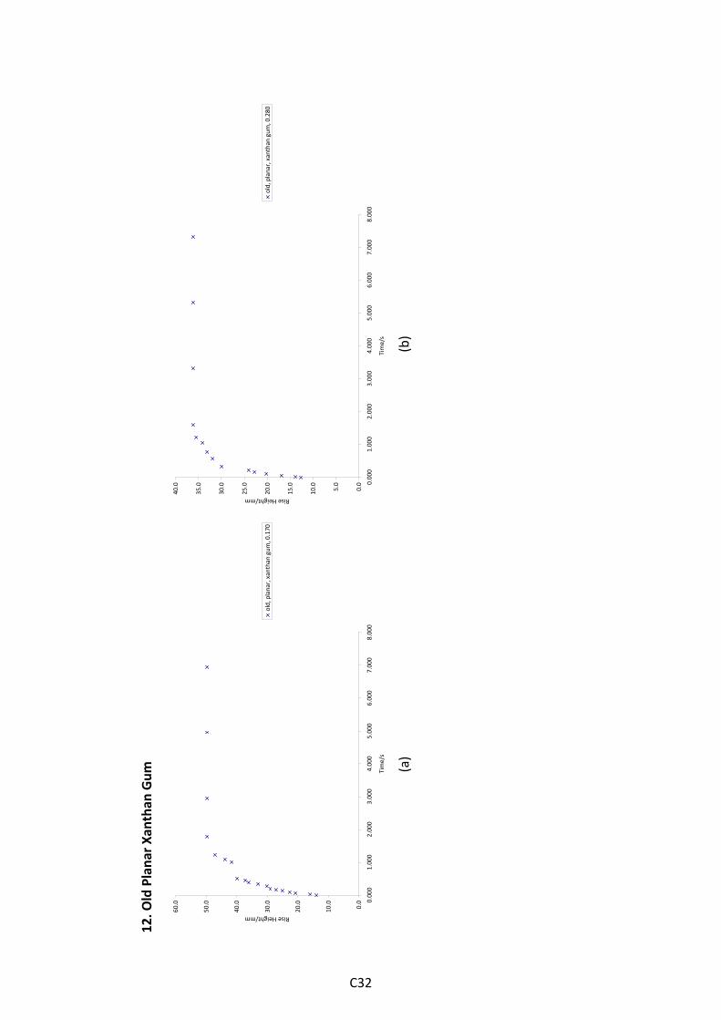
12. O

ld Plana

r Xa

ntha

n Gum

  

0.0

10.0

20.0

30.0

40.0

50.0

60.0 0.

000

1.000

2.000

3.000

4.000

5.000

6.000

7.000

8.000

Time/s

Rise Height/mm

old, planar, xanthan

 gum

, 0.170

 

0.0

5.0

10.0

15.0

20.0

25.0

30.0

35.0

40.0 0.

000

1.000

2.000

3.000

4.000

5.000

6.000

7.000

8.000

Time/s

Rise Height/mm

old, planar, xanthan

 gum

, 0.280

  

  

         (a) 

  

  

  

  

    (b

)   

C32

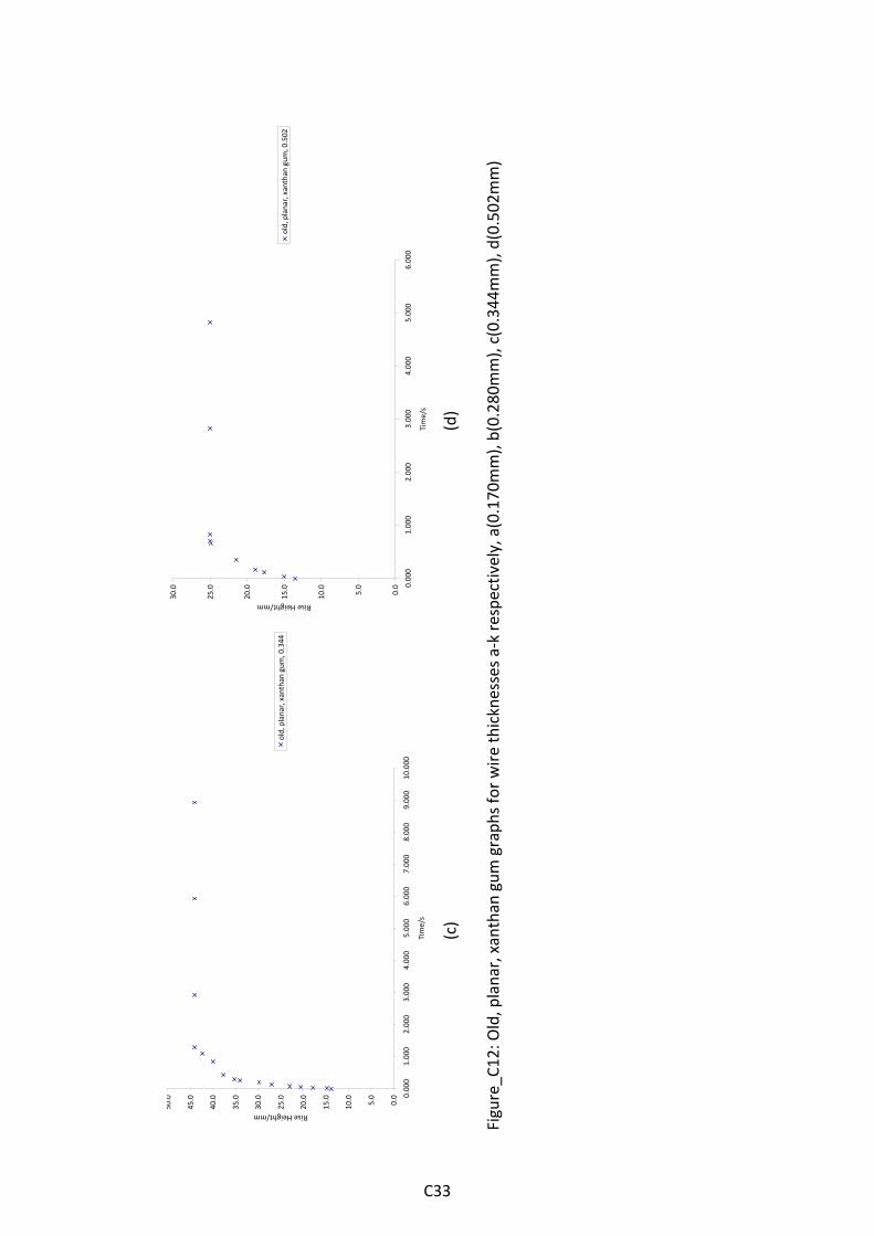
0.0

5.0

10.0

15.0

20.0

25.0

30.0

35.0

40.0

45.0

50.0 0.

000

1.000

2.000

3.000

4.000

5.000

6.000

7.000

8.000

9.000

10.000

Time/s

Rise Height/mm

old, planar, xanthan

 gum

, 0.344

 

0.0

5.0

10.0

15.0

20.0

25.0

30.0 0.

000

1.000

2.000

3.000

4.000

5.000

6.000

Time/s

Rise Height/mm

old, planar, xanthan

 gum

, 0.502

  

  

        (c)  

  

  

  

  

   (d) 

  Figure_C

12: O

ld, planar, xanthan

 gum

 graph

s for wire thicknesses a‐k respectiv

ely, a(0.170mm), b(0.28

0mm), c(0.344m

m), d(0.502m

m) 

                         

C33

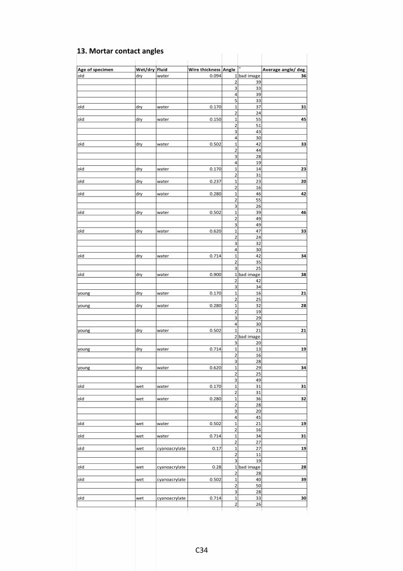
13. Mortar contact angles  Age of specimen Wet/dry Fluid Wire thickness Angle  ˚ Average angle/ degold dry water 0.094 1 bad image 36

2 393 334 395 33

old dry water 0.170 1 37 312 24

old  dry water 0.150 1 55 452 513 434 30

old dry water 0.502 1 42 332 443 284 19

old dry water 0.170 1 14 232 31

old dry water 0.237 1 23 202 16

old dry water 0.280 1 46 422 553 26

old dry water 0.502 1 39 462 493 49

old dry water 0.620 1 47 332 243 324 30

old dry water 0.714 1 42 342 353 25

old dry water 0.900 1 bad image 382 423 34

young dry water 0.170 1 16 212 25

young dry water 0.280 1 32 282 193 294 30

young dry water 0.502 1 21 212 bad image3 20

young dry water 0.714 1 13 192 163 28

young dry water 0.620 1 29 342 253 49

old wet water 0.170 1 31 312 31

old wet water 0.280 1 36 322 283 204 45

old wet water 0.502 1 21 192 16

old wet water 0.714 1 34 312 27

old wet cyanoacrylate 0.17 1 27 192 113 19

old wet cyanoacrylate 0.28 1 bad image 282 28

old wet cyanoacrylate 0.502 1 40 392 503 28

old wet cyanoacrylate 0.714 1 33 302 26

 

C34

D1  

APPENDIX D  

Numerical Models and CDs  

   

1. Planar experimental videos 2. Tapered experimental videos 3. Tortuous and natural experimental videos 4. Planar and tapered flow model