an introduction to nonlinear mixed effects models and …davidian/webinar.pdf · • a formal...
TRANSCRIPT
An Introduction to NonlinearMixed Effects Models and PK/PD
Analysis
Marie Davidian
Department of Statistics
North Carolina State University
http://www.stat.ncsu.edu/∼davidian
1

Outline
1. Introduction
2. Pharmacokinetics and pharmacodynamics
3. Model formulation
4. Model interpretation and inferential objectives
5. Inferential approaches
6. Applications
7. Extensions
8. Discussion
2
Some references
Material in this webinar is drawn from:
Davidian, M. and Giltinan, D.M. (1995). Nonlinear Models for Repeated
Measurement Data. Chapman & Hall/CRC Press.
Davidian, M. and Giltinan, D.M. (2003). Nonlinear models for repeated
measurement data: An overview and update. Journal of Agricultural,
Biological, and Environmental Statistics 8, 387–419.
Davidian, M. (2009). Non-linear mixed-effects models. In Longitudinal Data
Analysis, G. Fitzmaurice, M. Davidian, G. Verbeke, and G. Molenberghs
(eds). Chapman & Hall/CRC Press, ch. 5, 107–141.
Shameless promotion:
3
Introduction
Common situation in the biosciences:
• A continuous outcome evolves over time (or other condition) within
individuals from a population of interest
• Scientific interest focuses on features or mechanisms that underlie
individual time trajectories of the outcome and how these vary
across the population
• A theoretical or empirical model for such individual profiles, typically
nonlinear in parameters that may be interpreted as representing such
features or mechanisms, is available
• Repeated measurements over time are available on each individual in
a sample drawn from the population
• Inference on the scientific questions of interest is to be made in the
context of the model and its parameters
4

Introduction
Nonlinear mixed effects model:
• Also known as the hierarchical nonlinear model
• A formal statistical framework for this situation
• Much statistical methodological research in the early 1990s
• Now widely accepted and used, with applications routinely reported
and commercial and free software available
• Extensions and methodological innovations are still ongoing
Objectives:
• Provide an introduction to the formulation, utility, and
implementation of nonlinear mixed models
• For definiteness, focus on pharmacokinetics and pharmacodynamics
as major application area
5

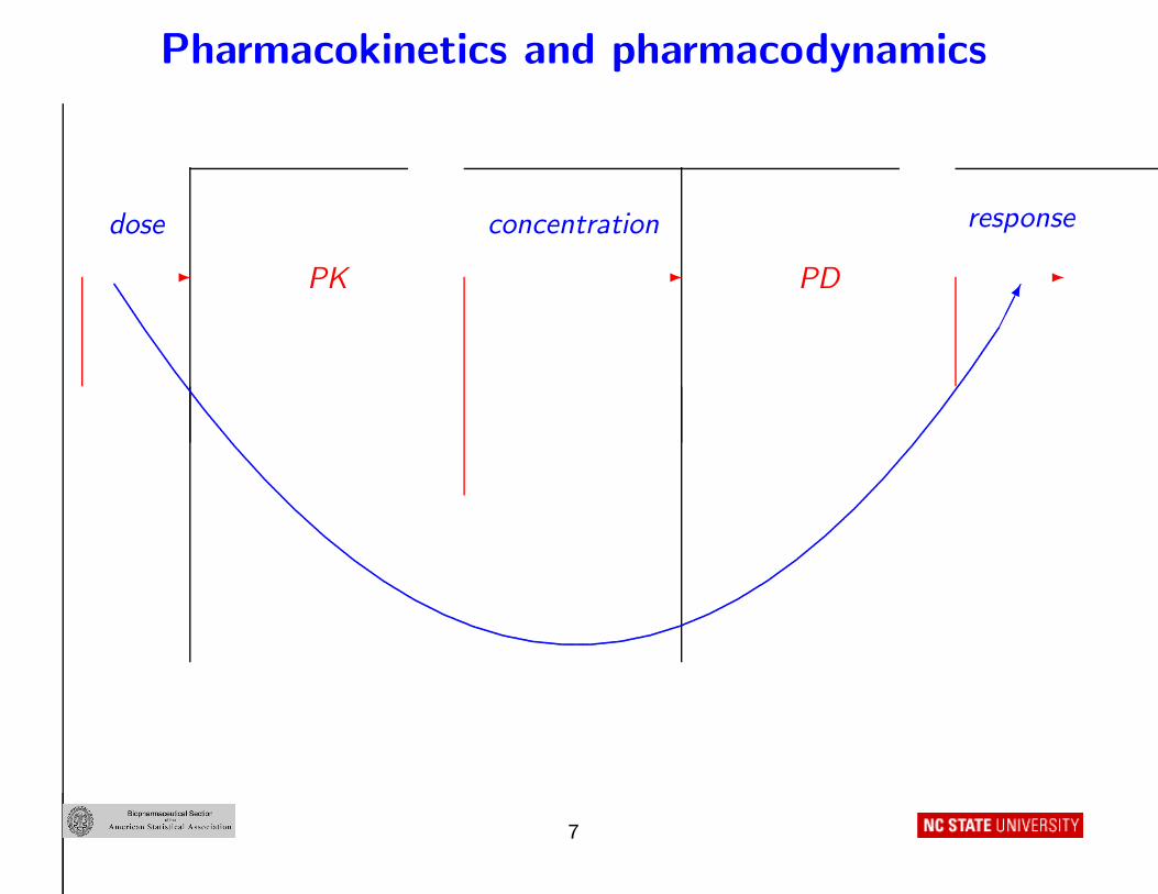
Pharmacokinetics and pharmacodynamics
Premise: Understanding what goes on between dose (administration)
and response can yield information on
• How best to choose doses at which to evaluate a drug
• Suitable dosing regimens to recommend to the population,
subpopulations of patients, and individual patients
• Labeling
Key concepts:
• Pharmacokinetics (PK ) – “what the body does to the drug”
• Pharmacodynamics (PD ) – “what the drug does to the body”
An outstanding overview: “Pharmacokinetics and
pharmacodynamics ,” by D.M. Giltinan, in Encyclopedia of Biostatistics,
2nd edition
6
Pharmacokinetics and pharmacodynamics
PK -
concentration
PD- -dose response
.
......................................................
...................................................
................................................
.............................................
..........................................
.......................................
......................................
.................
.................
...
..................
..................
......................
.............
........................
..........
..............................
...
................................
...............................
.............................. ............................. .............................................................
................................
.................................
..................................
...................................
....................................
.....................................
......................................
.......................................
..........................................
.............................................
................................................
...................................................
���
7
Pharmacokinetics and pharmacodynamics
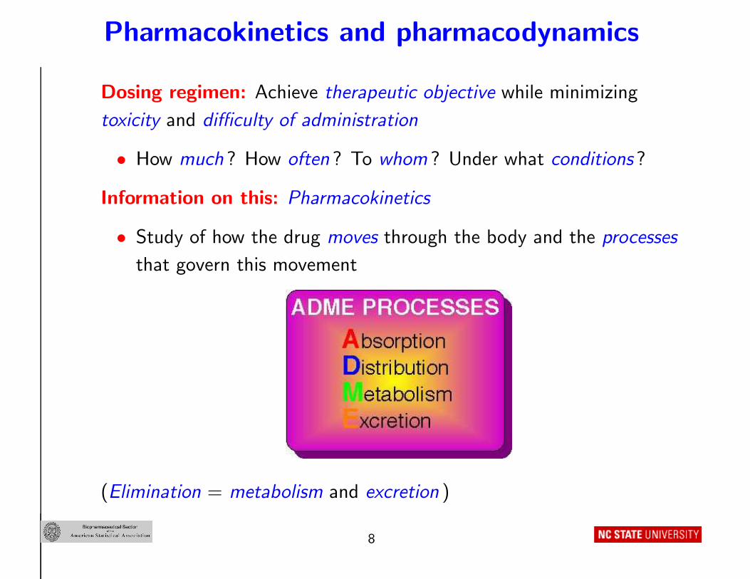
Dosing regimen: Achieve therapeutic objective while minimizing
toxicity and difficulty of administration
• How much ? How often ? To whom ? Under what conditions ?
Information on this: Pharmacokinetics
• Study of how the drug moves through the body and the processes
that govern this movement
(Elimination = metabolism and excretion )
8

Pharmacokinetics and pharmacodynamics
Basic assumptions and principles:
• There is an “effect site ” where drug will have its effect
• Magnitudes of response and toxicity depend on drug concentration
at the effect site
• Drug cannot be placed directly at effect site, must move there
• Concentrations at the effect site are determined by ADME
• Concentrations must be kept high enough to produce a desirable
response, but low enough to avoid toxicity
=⇒ “Therapeutic window ”
• (Usually ) cannot measure concentration at effect site directly, but
can measure in blood/plasma/serum; reflect those at site
9
Pharmacokinetics and pharmacodynamics
Pharmacokinetics (PK): First part of the story
• Broad goal of PK analysis : Understand and characterize
intra-subject ADME processes of drug absorption , distribution ,
metabolism and excretion (elimination ) governing achieved drug
concentrations
• . . . and how these processes vary across subjects (inter-subject
variation )
10

Pharmacokinetics and pharmacodynamics
PK studies in humans: “Intensive studies ”
• Small number of subjects (often healthy volunteers )
• Frequent samples over time, often following single dose
• Usually early in drug development
• Useful for gaining initial information on “typical ” PK behavior in
humans and for identifying an appropriate PK model. . .
• Preclinical PK studies in animals are generally intensive studies
11
Pharmacokinetics and pharmacodynamics
PK studies in humans: “Population studies ”
• Large number of subjects (heterogeneous patients)
• Often in later stages of drug development or after a drug is in
routine use
• Haphazard , sparse sampling over time, multiple dosing intervals
• Extensive demographic and physiologic characteristics
• Useful for understanding associations between patient characteristics
and PK behavior =⇒ tailored dosing recommendations
12
Pharmacokinetics and pharmacodynamics
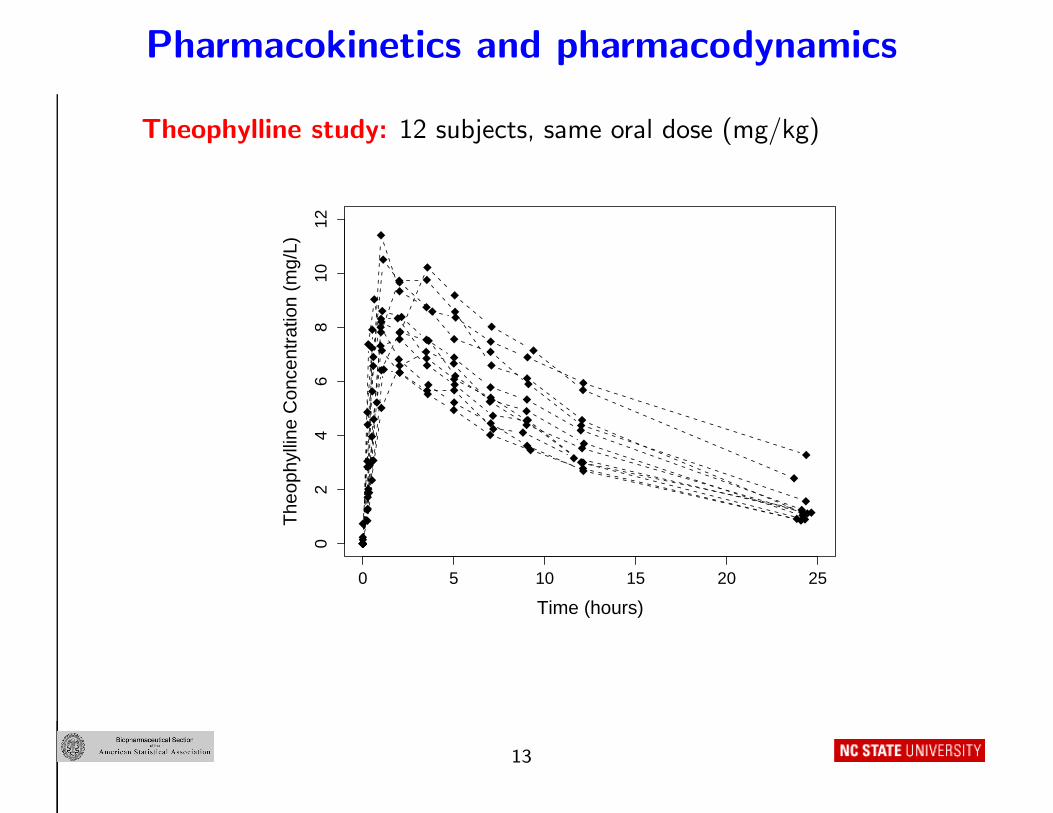
Theophylline study: 12 subjects, same oral dose (mg/kg)
0 5 10 15 20 25
02
46
810
12
Time (hours)
The
ophy
lline
Con
cent
ratio
n (m
g/L)
13
Pharmacokinetics and pharmacodynamics
Features:
• Intensive study
• Similarly shaped concentration-time profiles across subjects
• . . . but peak, rise, decay vary
• Attributable to inter-subject variation in underlying PK behavior
(absorption, distribution, elimination)
Standard: Represent the body by a simple system of compartments
• Gross simplification but extraordinarily useful. . .
14

Pharmacokinetics and pharmacodynamics
One-compartment model with first-order absorption, elimination:
oral dose D A(t) --
keka
dA(t)
dt= kaAa(t) − keA(t), A(0) = 0
dAa(t)
dt= −kaAa(t), Aa(0) = D
F = bioavailability, Aa(t) = amount at absorption site
Concentration at t : m(t) =A(t)
V=
kaDF
V (ka − ke){exp(−ket) − exp(−kat)},
ke = Cl/V, V = “volume ” of compartment, Cl = clearance
15
Pharmacokinetics and pharmacodynamics
One-compartment model for theophylline:
• Single “blood compartment ” with fractional rates of absorption ka
and elimination ke
• Deterministic mathematical model
• Individual PK behavior characterized by PK parameters
θ = (ka, V, Cl)′
By-product:
• The PK model assumes PK processes are dose-independent
• =⇒ Knowledge of the values of θ = (ka, V, Cl)′ allows
determination of concentrations achieved at any time t under
different doses
• Can be used to develop dosing regimens
16
Pharmacokinetics and pharmacodynamics
Objectives of analysis:
• Estimate “typical ” values of θ = (ka, V, Cl)′ and how they vary in
the population of subjects based on the longitudinal concentration
data from the sample of 12 subjects
• =⇒ Must incorporate the (theoretical ) PK model in an appropriate
statistical model (somehow. . . )
17
Pharmacokinetics and pharmacodynamics
Quinidine population PK study: N = 136 patients undergoing
treatment with oral quinidine for atrial fibrillation or arrhythmia
• Demographic/physiologic characteristics : Age, weight, height,
ethnicity/race, smoking status, ethanol abuse, congestive heart
failure, creatinine clearance, α1-acid glycoprotein concentration, . . .
• Samples taken over multiple dosing intervals =⇒(dose time, amount) = (sℓ, Dℓ) for the ℓth dose interval
• Standard assumption: “Principle of superposition ” =⇒ multiple
doses are “additive ”
• One compartment model gives expression for concentration
at time t. . .
18

Pharmacokinetics and pharmacodynamics
For a subject not yet at a steady state:
Aa(sℓ) = Aa(sℓ−1) exp{−ka(sℓ − sℓ−1)} + Dℓ,
m(sℓ) = m(sℓ−1) exp{−ke(sℓ − sℓ−1)} + Aa(sℓ−1)ka
V (ka − ke)
×[exp{−ke(sℓ − sℓ−1)} − exp{−ka(sℓ − sℓ−1)}
].
m(t) = m(sℓ) exp{−ke(t − sℓ)} + Aa(sℓ)ka
V (ka − ke)
×[exp{−ke(t − sℓ)} − exp{−ka(t − sℓ)}
], sℓ < t < sℓ+1
ke = Cl/V, θ = (ka, V, Cl)′
Objective of analysis: Characterize typical values of and variation in
θ = (ka, V, Cl)′ across the population and elucidate systematic
associations between θ and patient characteristics
19
Pharmacokinetics and pharmacodynamics
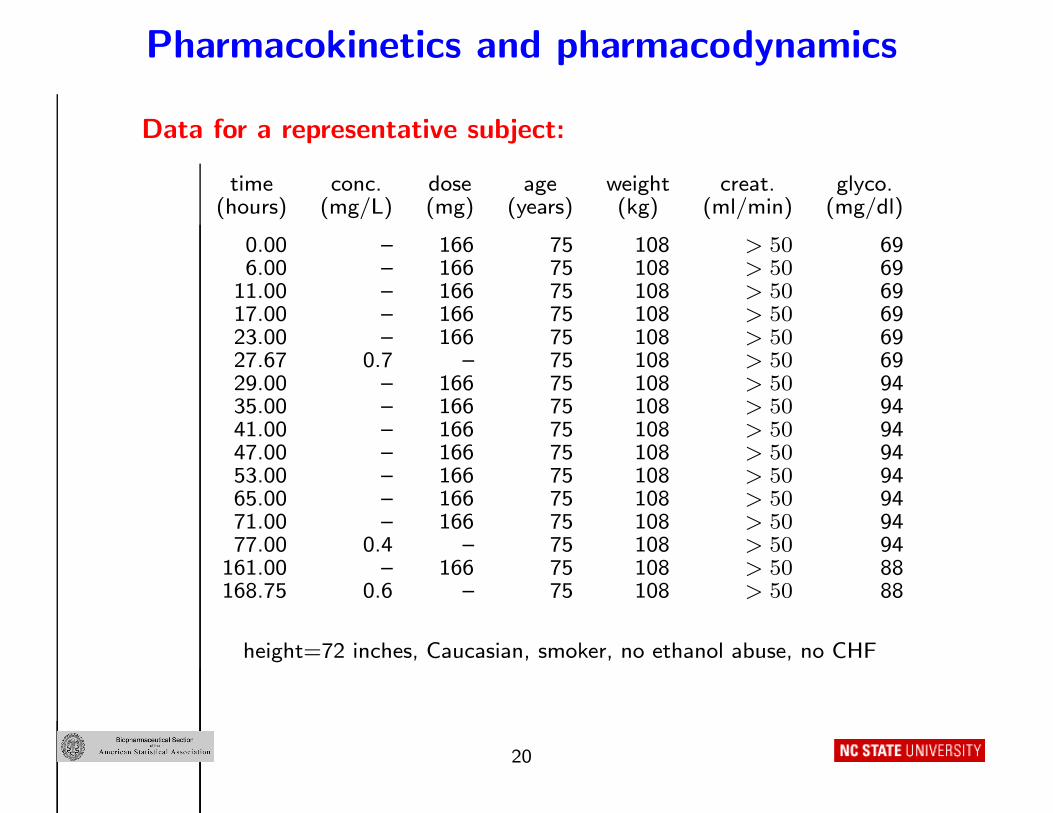
Data for a representative subject:
time conc. dose age weight creat. glyco.(hours) (mg/L) (mg) (years) (kg) (ml/min) (mg/dl)
0.00 – 166 75 108 > 50 696.00 – 166 75 108 > 50 69
11.00 – 166 75 108 > 50 6917.00 – 166 75 108 > 50 6923.00 – 166 75 108 > 50 6927.67 0.7 – 75 108 > 50 6929.00 – 166 75 108 > 50 9435.00 – 166 75 108 > 50 9441.00 – 166 75 108 > 50 9447.00 – 166 75 108 > 50 9453.00 – 166 75 108 > 50 9465.00 – 166 75 108 > 50 9471.00 – 166 75 108 > 50 9477.00 0.4 – 75 108 > 50 94
161.00 – 166 75 108 > 50 88168.75 0.6 – 75 108 > 50 88
height=72 inches, Caucasian, smoker, no ethanol abuse, no CHF
20

Pharmacokinetics and pharmacodynamics
Pharmacodynamics (PD): Second part of the story
• What is a “good ” drug concentration?
• What is the “therapeutic window ?” Is it wide or narrow ? Is it the
same for everyone ?
• Relationship of response to drug concentration
• PK/PD study : Collect both concentration and response data from
each subject
21
Pharmacokinetics and pharmacodynamics
Argatroban PK/PD study: Anticoagulant
• N = 37 subjects assigned to different constant infusion rates
(doses) of 1 to 5 µ/kg/min of argatroban
• Administered by intravenous infusion for 4 hours (240 min)
• PK (blood samples) at
(30,60,90,115,160,200,240,245,250,260,275,295,320) min
• PD : additional samples at 5–9 time points, measured activated
partial thromboplastin time (aPTT, the response)
Effect site: The blood
22
Pharmacokinetics and pharmacodynamics
0 100 200 300
020
040
060
080
010
0012
00
Time (min)
Arg
atro
ban
Con
cent
ratio
n (n
g/m
l)
Infusion rate 1.0 µg/kg/min
0 100 200 300
020
040
060
080
010
0012
00
Time (min)
Arg
atro
ban
Con
cent
ratio
n (n
g/m
l)
Infustion rate 4.5 µg/kg/min
23
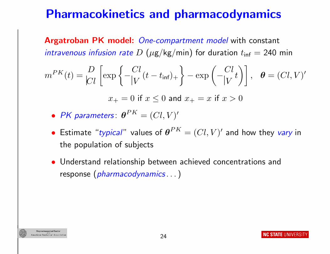
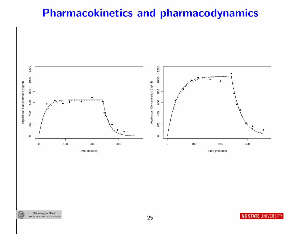
Pharmacokinetics and pharmacodynamics
Argatroban PK model: One-compartment model with constant
intravenous infusion rate D (µg/kg/min) for duration tinf = 240 min
mPK(t) =D
Cl
[exp
{−Cl
V(t − tinf)+
}− exp
(−Cl
Vt
)], θ = (Cl, V )′
x+ = 0 if x ≤ 0 and x+ = x if x > 0
• PK parameters : θPK = (Cl, V )′
• Estimate “typical ” values of θPK = (Cl, V )′ and how they vary in
the population of subjects
• Understand relationship between achieved concentrations and
response (pharmacodynamics . . . )
24
Pharmacokinetics and pharmacodynamics
0 100 200 300
020
040
060
080
010
0012
00
Time (minutes)
Arg
atro
ban
Con
cent
ratio
n (n
g/m
l)
0 100 200 300
020
040
060
080
010
0012
00
Time (minutes)A
rgat
roba
n C
once
ntra
tion
(ng/
ml)
25
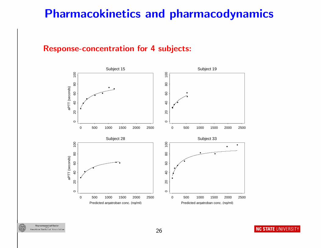
Pharmacokinetics and pharmacodynamics
Response-concentration for 4 subjects:
aPT
T (
seco
nds)
0 500 1000 1500 2000 2500
020
4060
8010
0Subject 15
0 500 1000 1500 2000 2500
020
4060
8010
0
Subject 19
Predicted argatroban conc. (ng/ml)
aPT
T (
seco
nds)
0 500 1000 1500 2000 2500
020
4060
8010
0
Subject 28
Predicted argatroban conc. (ng/ml)
0 500 1000 1500 2000 2500
020
4060
8010
0
Subject 33
26

Pharmacokinetics and pharmacodynamics
Argatroban PD model: “Emax model ”
mPD(t) = E0 +Emax − E0
1 + EC50/mPK(t)
• Response at time t depends on concentration at effect site at time t
(same as concentration in blood here)
• PD parameters : θPD = (E0, Emax, EC50)′
• Also depends on PK parameters
• Estimate “typical ” values of θPD = (E0, Emax, EC50)′ and how
they vary in the population of subjects
27

Pharmacokinetics and pharmacodynamics
Ultimate objective: Put PK and PD together to
• Characterize the “therapeutic window ” and how it varies across
subjects
• Develop dosing regimens targeting achieved concentrations leading
to therapeutic response
• For population, subpopulations, individuals
• Decide on dose(s) to carry forward to future studies
28
Pharmacokinetics and pharmacodynamics
Summary: Common themes
• An outcome (or outcomes) evolves over time; e.g., concentration in
PK, response in PD
• Interest focuses on underlying mechanisms/processes taking place
within an individual leading to outcome trajectories and how these
vary across the population
• A (usually deterministic ) model is available representing
mechanisms explicitly by scientifically meaningful model parameters
• Mechanisms cannot be observed directly
• =⇒ Inference on mechanisms must be based on repeated
measurements of the outcome(s) over time on each of a sample of
N individuals from the population
29
Pharmacokinetics and pharmacodynamics
Other application areas:
• Toxicokinetics (Physiologically-based pharmacokinetic – PBPK –
models)
• HIV dynamics
• Stability testing
• Agriculture
• Forestry
• Dairy science
• Cancer dynamics
• More . . .
30
Model formulation
Nonlinear mixed effects model: Embed the (deterministic ) model
describing individual trajectories in a statistical model
• Formalizes knowledge and assumptions about variation in outcomes
and mechanisms within and among individuals
• Provides a framework for inference based on repeated measurement
data from N individuals
• For simplicity : Focus on univariate outcome (= drug concentration
in PK); multivariate (PK/PD ) outcome later
Basic set-up: N individuals from a population of interest, i = 1, . . . , N
• For individual i, observe ni measurements of the outcome
Yi1, Yi2, . . . , Yiniat times ti1, ti2, . . . , tini
• I.e., for individual i, Yij at time tij , j = 1, . . . , ni
31
Model formulation
Within-individual conditions of observation: For individual i, U i
• Theophylline : U i = Di = oral dose for i at time 0 (mg/kg)
• Argatroban : U i = (Di, tinf) = infusion rate and duration for i
• Quinidine : For subject i observed over di dosing intervals, U i has
elements (siℓ, Diℓ)′, ℓ = 1, . . . , di
• U i are “within-individual covariates ” – needed to describe
outcome-time relationship at the individual level
32
Model formulation
Individual characteristics: For individual i, Ai
• Age, weight, ethnicity, smoking status, renal function, etc. . .
• For now : Elements of Ai do not change over observation period
• Ai are “among-individual covariates ” – relevant only to how
individuals differ but are not needed to describe outcome-time
relationship at the individual level
Observed data: (Y ′
i, X′
i)′, i = 1, . . . , N , assumed independent across i
• Y i = (Yi1, . . . , Yini)′
• Xi = (U ′
i, A′
i)′ = combined within- and among-individual
covariates (for brevity later)
Basic model: A two-stage hierarchy
33

Model formulation
Stage 1 – Individual-level model:
Yij = m(tij , U i, θi) + eij , j = 1, . . . , ni, θi (r × 1)
• E.g., for theophylline (F ≡ 1)
m(t, U i, θi) =kaiDi
Vi(kai − Cli/Vi){exp(−Clit/Vi) − exp(−kait)}
θi = (kai, Vi, Cli)′ = (θi1, θi2, θi3)
′, r = 3, U i = Di
• Assume eij = Yij − m(tij , U i, θi) satisfy E(eij |U i, θi) = 0
=⇒ E(Yij |U i, θi) = m(tij , U i, θi) for each j
• Standard assumption : eij and hence Yij are conditionally normally
distributed (on U i, θi)
• More shortly. . .
34
Model formulation
Stage 2 – Population model:
θi = d(Ai, β, bi), i = 1, . . . , N, (r × 1)
• d is r-dimensional function describing relationship between θi and
Ai in terms of . . .
• β (p × 1) fixed parameter (“fixed effects ”)
• bi (q × 1) “random effects ”
• Characterizes how elements of θi vary across individual due to
– Systematic associations with Ai (modeled via β)
– “Unexplained variation ” in the population (represented by bi)
• Usual assumptions :
E(bi |Ai) = E(bi) = 0 and Cov(bi |Ai) = Cov(bi) = G, bi ∼ N(0, G)
35
Model formulation
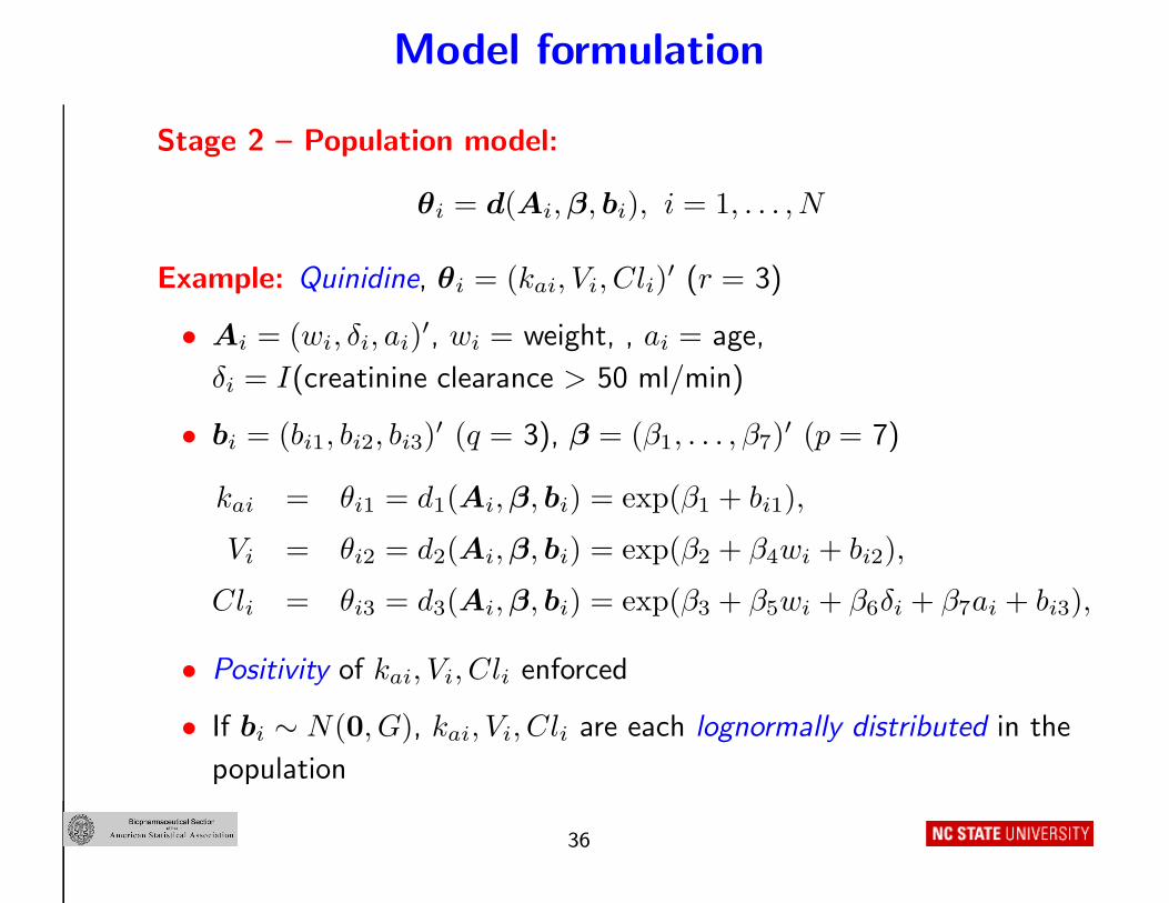
Stage 2 – Population model:
θi = d(Ai, β, bi), i = 1, . . . , N
Example: Quinidine, θi = (kai, Vi, Cli)′ (r = 3)
• Ai = (wi, δi, ai)′, wi = weight, , ai = age,
δi = I(creatinine clearance > 50 ml/min)
• bi = (bi1, bi2, bi3)′ (q = 3), β = (β1, . . . , β7)
′ (p = 7)
kai = θi1 = d1(Ai, β, bi) = exp(β1 + bi1),
Vi = θi2 = d2(Ai, β, bi) = exp(β2 + β4wi + bi2),
Cli = θi3 = d3(Ai, β, bi) = exp(β3 + β5wi + β6δi + β7ai + bi3),
• Positivity of kai, Vi, Cli enforced
• If bi ∼ N(0, G), kai, Vi, Cli are each lognormally distributed in the
population
36

Model formulation
Stage 2 – Population model:
θi = d(Ai, β, bi), i = 1, . . . , N
Example: Quinidine, continued, θi = (kai, Vi, Cli)′ (r = 3)
• “Are elements of θi fixed or random effects ?”
• “Unexplained variation ” in one component of θi “small ” relative to
others – no associated random effect, e.g., r = 3, q = 2
kai = exp(β1 + bi1)
Vi = exp(β2 + β4wi) (all population variation due to weight)
Cli = exp(β3 + β5wi + β6δi + β7ai + bi3)
• An approximation – usually biologically implausible ; used for
parsimony, numerical stability
37

Model formulation
Stage 2 – Population model:
θi = d(Ai, β, bi), i = 1, . . . , N
• Allows nonlinear (in β and bi) specifications for elements of θi
• May be more appropriate than linear specifications (positivity
requirements, skewed distributions)
Some accounts: Restrict to linear specification
θi = Aiβ + Bibi
• Ai (r × p) “design matrix ” depending on elements of Ai
• Bi (r × q) typically 0s and 1s (identity matrix if r = q)
• Mainly in the statistical literature
38
Model formulation
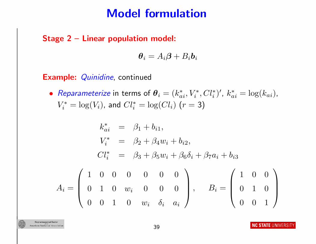
Stage 2 – Linear population model:
θi = Aiβ + Bibi
Example: Quinidine, continued
• Reparameterize in terms of θi = (k∗
ai, V∗
i , Cl∗i )′, k∗
ai = log(kai),
V ∗
i = log(Vi), and Cl∗i = log(Cli) (r = 3)
k∗
ai = β1 + bi1,
V ∗
i = β2 + β4wi + bi2,
Cl∗i = β3 + β5wi + β6δi + β7ai + bi3
Ai =
1 0 0 0 0 0 0
0 1 0 wi 0 0 0
0 0 1 0 wi δi ai
, Bi =
1 0 0
0 1 0
0 0 1
39

Model formulation
Stage 2 – Population model:
θi = d(Ai, β, bi), i = 1, . . . , N
Simplest example: Argatroban PK - No among-individual covariates
• θPKi = (Cli, Vi)
′ (r = 2), take
Cli = exp(β1 + bi1)
Vi = exp(β2 + bi2)
• Or reparameterize with θPKi = (Cl∗i , V ∗
i )′, Cl∗i = log(Cli),
V ∗
i = log(Vi)
Cl∗i = β1 + bi1
V ∗
i = β2 + bi2
so Ai = Bi = (2 × 2) identity matrix
40

Model formulation
Within-individual considerations: Complete the Stage 1
individual-level model
• Assumptions on the distribution of Y i given U i and θi
• Focus on a single individual i observed under conditions U i
• Yij at times tij viewed as intermittent observations on a
stochastic process
Yi(t, U i) = m(t, U i, θi) + ei(t, U i)
E{ei(t, U i) |U i, θi} = 0, E{Yi(t, U i) |U i, θi} = m(t, U i, θi) for all t
• Yij = Yi(tij , U i), eij = ei(tij , U i)
• “Deviation ” process ei(t, U i) represents all sources of variation
acting within an individual causing a realization of Yi(t, U i) to
deviate from the “smooth ” trajectory m(t, U i, θi)
41

Model formulation
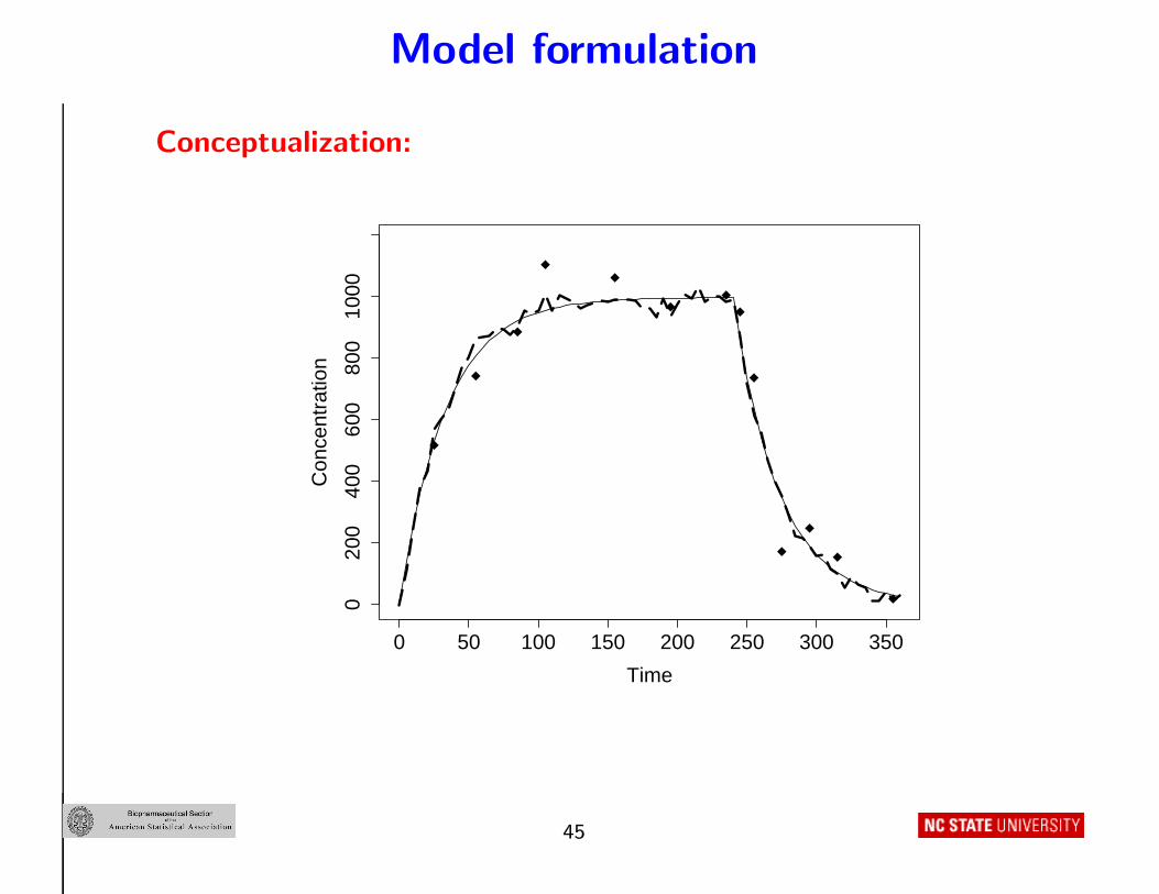
Conceptualization:
0 50 100 150 200 250 300 350
020
040
060
080
010
00
Time
Con
cent
ratio
n
42
Model formulation
Conceptual interpretation:
• Solid line : m(t, U i, θi) represents “inherent tendency ” for i’s
outcome to evolve over time; depends on i’s “inherent
characteristics ” θi
• Dashed line : Actual realization of the outcome – fluctuates about
solid line because m(t, U i, θi) is a simplification of complex truth
• Symbols : Actual, intermittent measurements of the dashed line –
deviate from the dashed line due to measurement error
Result: Two sources of intra-individual variation
• “Realization deviation ”
• Measurement error variation
• m(t, U i, θi) is the average of all possible realizations of measured
outcome trajectory that could be observed on i
43
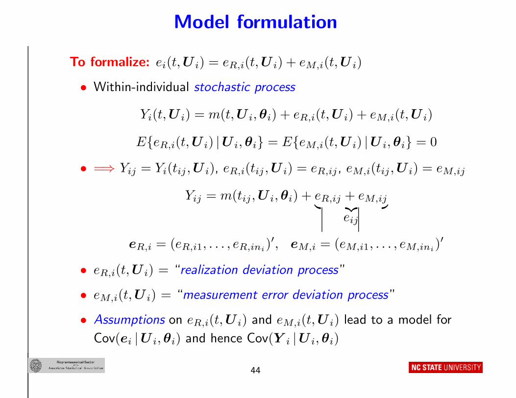
Model formulation
To formalize: ei(t, U i) = eR,i(t, U i) + eM,i(t, U i)
• Within-individual stochastic process
Yi(t, U i) = m(t, U i, θi) + eR,i(t, U i) + eM,i(t, U i)
E{eR,i(t, U i) |U i, θi} = E{eM,i(t, U i) |U i, θi} = 0
• =⇒ Yij = Yi(tij , U i), eR,i(tij , U i) = eR,ij, eM,i(tij , U i) = eM,ij
Yij = m(tij , U i, θi) + eR,ij + eM,ij︸ ︷︷ ︸eij
eR,i = (eR,i1, . . . , eR,ini)′, eM,i = (eM,i1, . . . , eM,ini
)′
• eR,i(t, U i) = “realization deviation process ”
• eM,i(t, U i) = “measurement error deviation process ”
• Assumptions on eR,i(t, U i) and eM,i(t, U i) lead to a model for
Cov(ei |U i, θi) and hence Cov(Y i |U i, θi)
44
Model formulation
Conceptualization:
0 50 100 150 200 250 300 350
020
040
060
080
010
00
Time
Con
cent
ratio
n
45
Model formulation
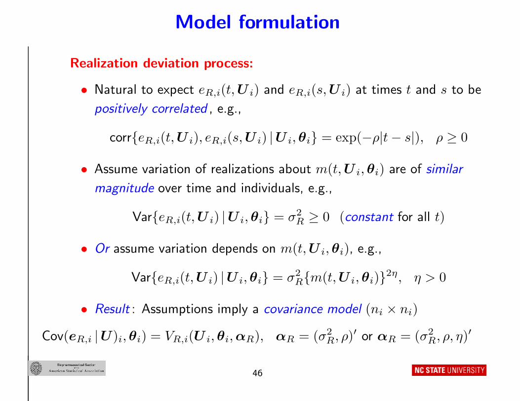
Realization deviation process:
• Natural to expect eR,i(t, U i) and eR,i(s, U i) at times t and s to be
positively correlated , e.g.,
corr{eR,i(t, U i), eR,i(s, U i) |U i, θi} = exp(−ρ|t − s|), ρ ≥ 0
• Assume variation of realizations about m(t, U i, θi) are of similar
magnitude over time and individuals, e.g.,
Var{eR,i(t, U i) |U i, θi} = σ2R ≥ 0 (constant for all t)
• Or assume variation depends on m(t, U i, θi), e.g.,
Var{eR,i(t, U i) |U i, θi} = σ2R{m(t, U i, θi)}2η, η > 0
• Result : Assumptions imply a covariance model (ni × ni)
Cov(eR,i |U)i, θi) = VR,i(U i, θi, αR), αR = (σ2R, ρ)′ or αR = (σ2
R, ρ, η)′
46

Model formulation
Conceptualization:
0 50 100 150 200 250 300 350
020
040
060
080
010
00
Time
Con
cent
ratio
n
47
Model formulation
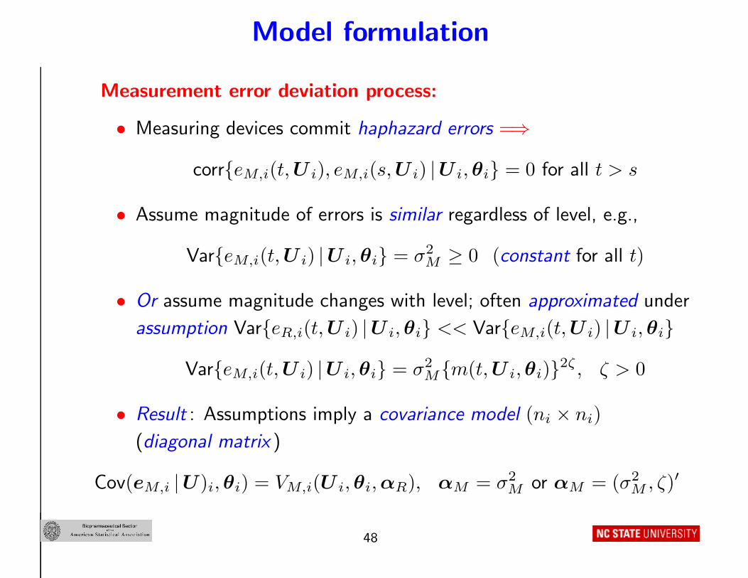
Measurement error deviation process:
• Measuring devices commit haphazard errors =⇒
corr{eM,i(t, U i), eM,i(s, U i) |U i, θi} = 0 for all t > s
• Assume magnitude of errors is similar regardless of level, e.g.,
Var{eM,i(t, U i) |U i, θi} = σ2M ≥ 0 (constant for all t)
• Or assume magnitude changes with level; often approximated under
assumption Var{eR,i(t, U i) |U i, θi} << Var{eM,i(t, U i) |U i, θi}
Var{eM,i(t, U i) |U i, θi} = σ2M{m(t, U i, θi)}2ζ , ζ > 0
• Result : Assumptions imply a covariance model (ni × ni)
(diagonal matrix )
Cov(eM,i |U)i, θi) = VM,i(U i, θi, αR), αM = σ2M or αM = (σ2
M , ζ)′
48

Model formulation
Combining:
• Standard assumption : eR,i(t, U i) and eM,i(t, U i) are independent
Cov(ei |U i, θi) = Cov(eR,i |U i, θi) + Cov(eM,i |U i, θi)
= VR,i(U i, θi, αR) + VM,i(U i, θi, αM )
= Vi(U i, θi, α)
α = (α′
R, α′
M )′
• This assumption may or may not be realistic
Practical considerations: Quite complex intra-individual covariance
models can result from faithful consideration of the situation. . .
• . . . But may be difficult to implement
49
Model formulation
Standard model simplifications: One or more might be adopted
• Negligible measurement error =⇒
Vi(U i, θi, α) = VR,i(U i, θi, αR)
• The tij may be at widely spaced intervals =⇒ autocorrelation
among eR,ij negligible =⇒ Vi(U i, θi, α) is diagonal
• Var{eR,i(t, U i) |U i, θi} << Var{eM,i(t, U i) |U i, θi} =⇒measurement error is dominant source
• Simplifications should be justifiable in the context at hand
Note: All of these considerations apply to any mixed effects model
formulation, not just nonlinear ones!
50
Model formulation
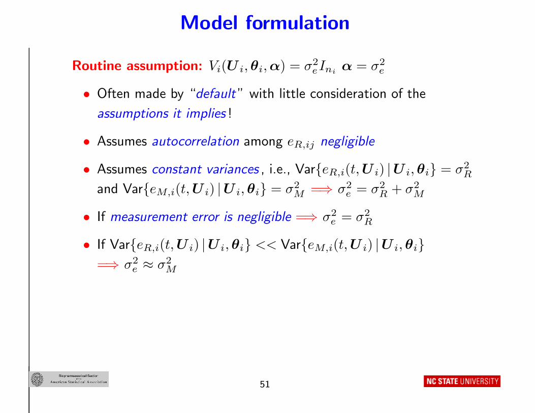
Routine assumption: Vi(U i, θi, α) = σ2eIni
α = σ2e
• Often made by “default ” with little consideration of the
assumptions it implies !
• Assumes autocorrelation among eR,ij negligible
• Assumes constant variances , i.e., Var{eR,i(t, U i) |U i, θi} = σ2R
and Var{eM,i(t, U i) |U i, θi} = σ2M =⇒ σ2
e = σ2R + σ2
M
• If measurement error is negligible =⇒ σ2e = σ2
R
• If Var{eR,i(t, U i) |U i, θi} << Var{eM,i(t, U i) |U i, θi}=⇒ σ2
e ≈ σ2M
51
Model formulation
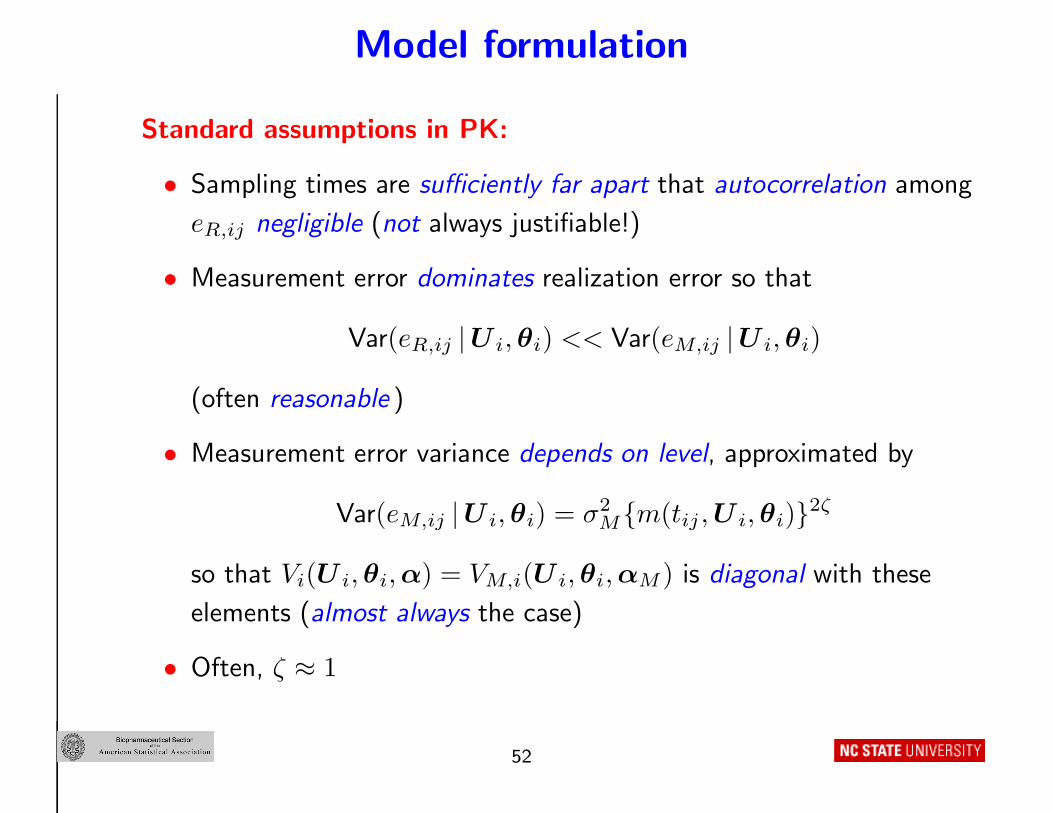
Standard assumptions in PK:
• Sampling times are sufficiently far apart that autocorrelation among
eR,ij negligible (not always justifiable!)
• Measurement error dominates realization error so that
Var(eR,ij |U i, θi) << Var(eM,ij |U i, θi)
(often reasonable )
• Measurement error variance depends on level, approximated by
Var(eM,ij |U i, θi) = σ2M{m(tij , U i, θi)}2ζ
so that Vi(U i, θi, α) = VM,i(U i, θi, αM ) is diagonal with these
elements (almost always the case)
• Often, ζ ≈ 1
52
Model formulation
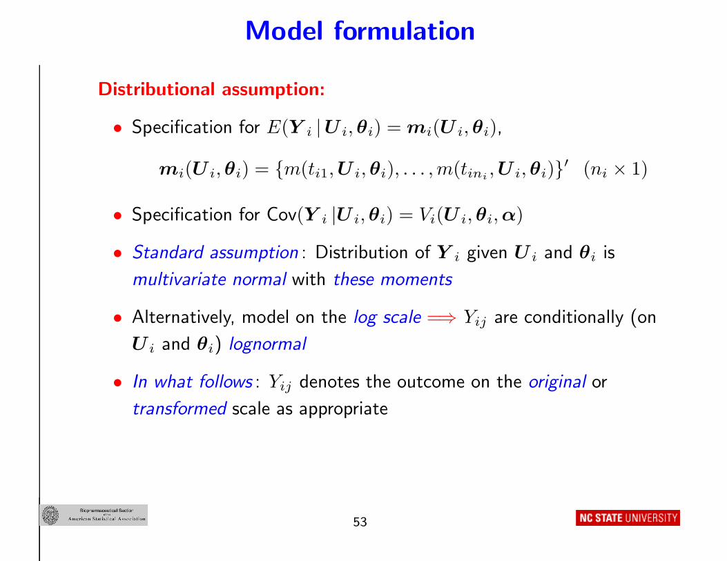
Distributional assumption:
• Specification for E(Y i |U i, θi) = mi(U i, θi),
mi(U i, θi) = {m(ti1, U i, θi), . . . , m(tini, U i, θi)}′ (ni × 1)
• Specification for Cov(Y i |U i, θi) = Vi(U i, θi, α)
• Standard assumption : Distribution of Y i given U i and θi is
multivariate normal with these moments
• Alternatively, model on the log scale =⇒ Yij are conditionally (on
U i and θi) lognormal
• In what follows : Yij denotes the outcome on the original or
transformed scale as appropriate
53
Model formulation
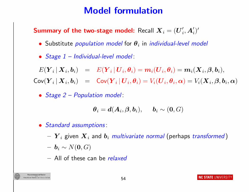
Summary of the two-stage model: Recall Xi = (U ′
i, A′
i)′
• Substitute population model for θi in individual-level model
• Stage 1 – Individual-level model :
E(Y i |Xi, bi) = E(Y i |U i, θi) = mi(U i, θi) = mi(Xi, β, bi),
Cov(Y i |Xi, bi) = Cov(Y i |U i, θi) = Vi(U i, θi, α) = Vi(Xi, β, bi, α)
• Stage 2 – Population model :
θi = d(Ai, β, bi), bi ∼ (0, G)
• Standard assumptions :
– Y i given Xi and bi multivariate normal (perhaps transformed )
– bi ∼ N(0, G)
– All of these can be relaxed
54
Model interpretation and inferential objectives
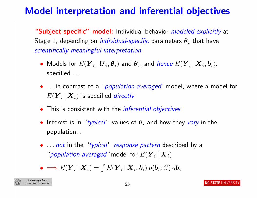
“Subject-specific” model: Individual behavior modeled explicitly at
Stage 1, depending on individual-specific parameters θi that have
scientifically meaningful interpretation
• Models for E(Y i |U i, θi) and θi, and hence E(Y i |Xi, bi),
specified . . .
• . . . in contrast to a “population-averaged ”model, where a model for
E(Y i |Xi) is specified directly
• This is consistent with the inferential objectives
• Interest is in “typical ” values of θi and how they vary in the
population. . .
• . . . not in the “typical ” response pattern described by a
“population-averaged ”model for E(Y i |Xi)
• =⇒ E(Y i |Xi) =∫
E(Y i |Xi, bi) p(bi; G) dbi
55
Model interpretation and inferential objectives
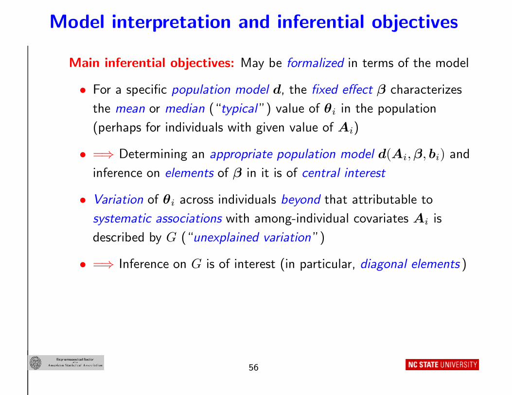
Main inferential objectives: May be formalized in terms of the model
• For a specific population model d, the fixed effect β characterizes
the mean or median (“typical ”) value of θi in the population
(perhaps for individuals with given value of Ai)
• =⇒ Determining an appropriate population model d(Ai, β, bi) and
inference on elements of β in it is of central interest
• Variation of θi across individuals beyond that attributable to
systematic associations with among-individual covariates Ai is
described by G (“unexplained variation ”)
• =⇒ Inference on G is of interest (in particular, diagonal elements )
56

Model interpretation and inferential objectives
Additional inferential objectives: In some contexts
• Inference on θi and/or m(t0, U i, θi) at some specific time t0 for
i = 1, . . . , N or for future individuals is of interest
• Example : “Individualized ” dosing in PK
• The model is a natural framework for “borrowing strength ” across
similar individuals (more later)
57
Inferential approaches
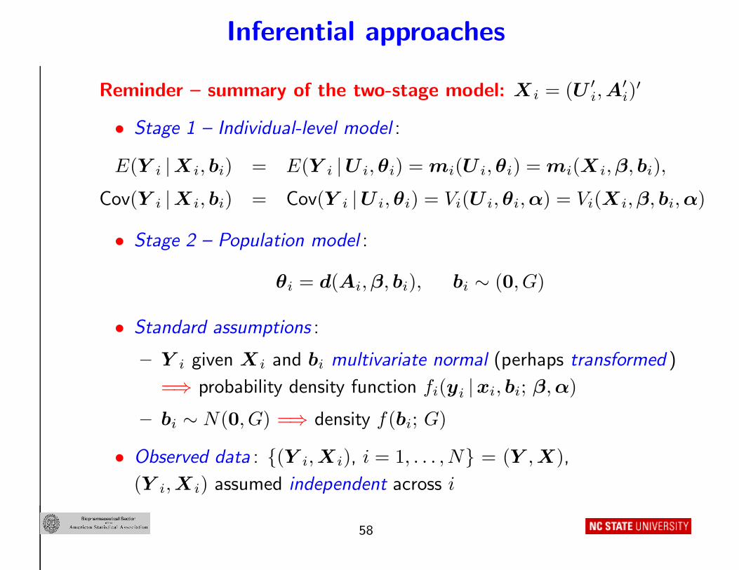
Reminder – summary of the two-stage model: Xi = (U ′
i, A′
i)′
• Stage 1 – Individual-level model :
E(Y i |Xi, bi) = E(Y i |U i, θi) = mi(U i, θi) = mi(Xi, β, bi),
Cov(Y i |Xi, bi) = Cov(Y i |U i, θi) = Vi(U i, θi, α) = Vi(Xi, β, bi, α)
• Stage 2 – Population model :
θi = d(Ai, β, bi), bi ∼ (0, G)
• Standard assumptions :
– Y i given Xi and bi multivariate normal (perhaps transformed )
=⇒ probability density function fi(yi |xi, bi; β, α)
– bi ∼ N(0, G) =⇒ density f(bi; G)
• Observed data : {(Y i, Xi), i = 1, . . . , N} = (Y , X),
(Y i, Xi) assumed independent across i
58
Inferential approaches
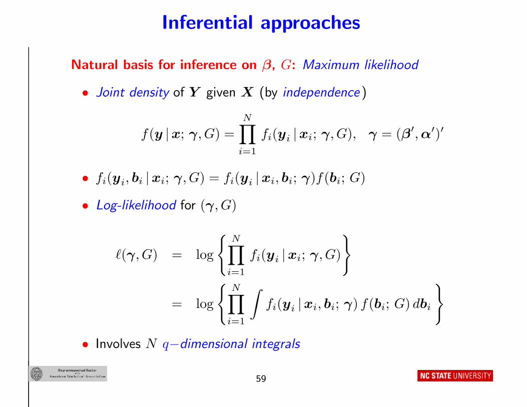
Natural basis for inference on β, G: Maximum likelihood
• Joint density of Y given X (by independence )
f(y |x; γ, G) =N∏
i=1
fi(yi |xi; γ, G), γ = (β′, α′)′
• fi(yi, bi |xi; γ, G) = fi(yi |xi, bi; γ)f(bi; G)
• Log-likelihood for (γ, G)
ℓ(γ, G) = log
{N∏
i=1
fi(yi |xi; γ, G)
}
= log
{N∏
i=1
∫fi(yi |xi, bi; γ) f(bi; G) dbi
}
• Involves N q−dimensional integrals
59
Inferential approaches
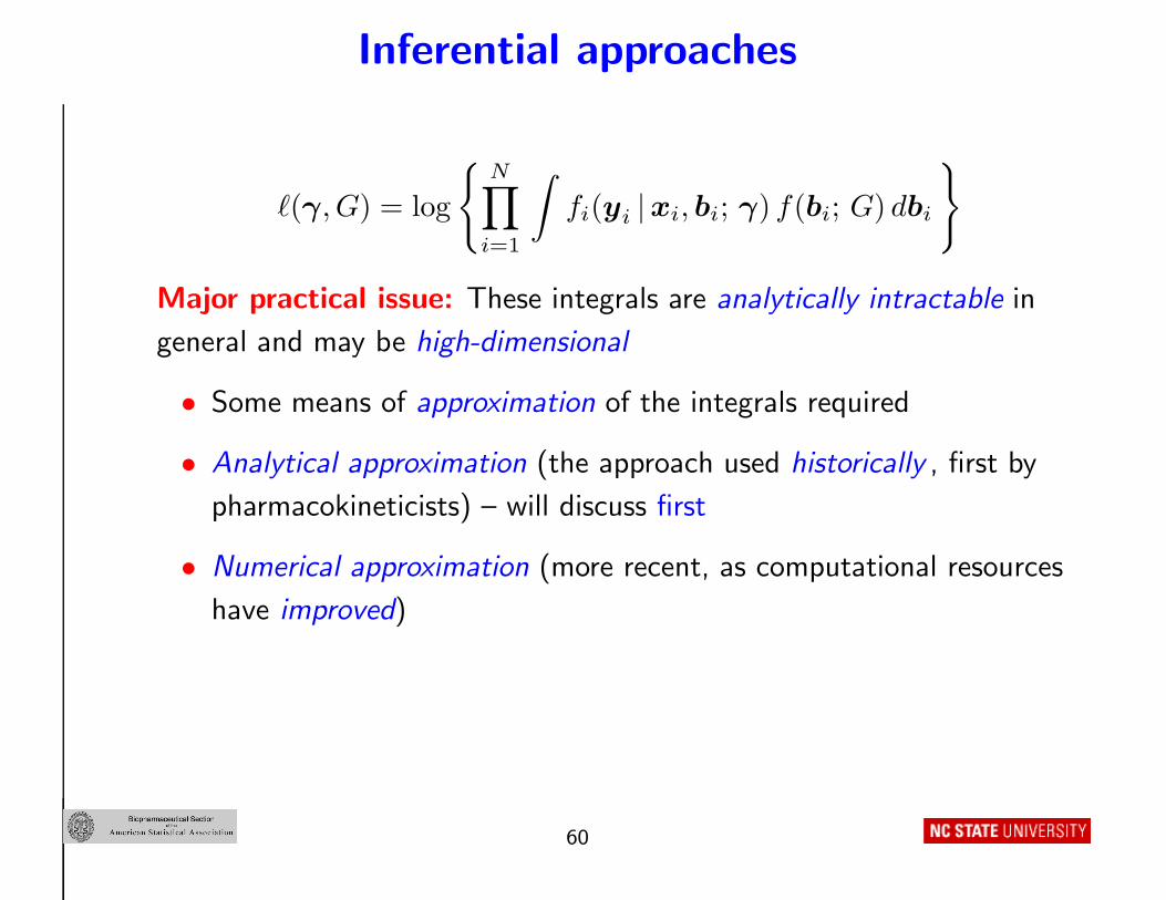
ℓ(γ, G) = log
{N∏
i=1
∫fi(yi |xi, bi; γ) f(bi; G) dbi
}
Major practical issue: These integrals are analytically intractable in
general and may be high-dimensional
• Some means of approximation of the integrals required
• Analytical approximation (the approach used historically , first by
pharmacokineticists) – will discuss first
• Numerical approximation (more recent, as computational resources
have improved)
60
Inferential approaches
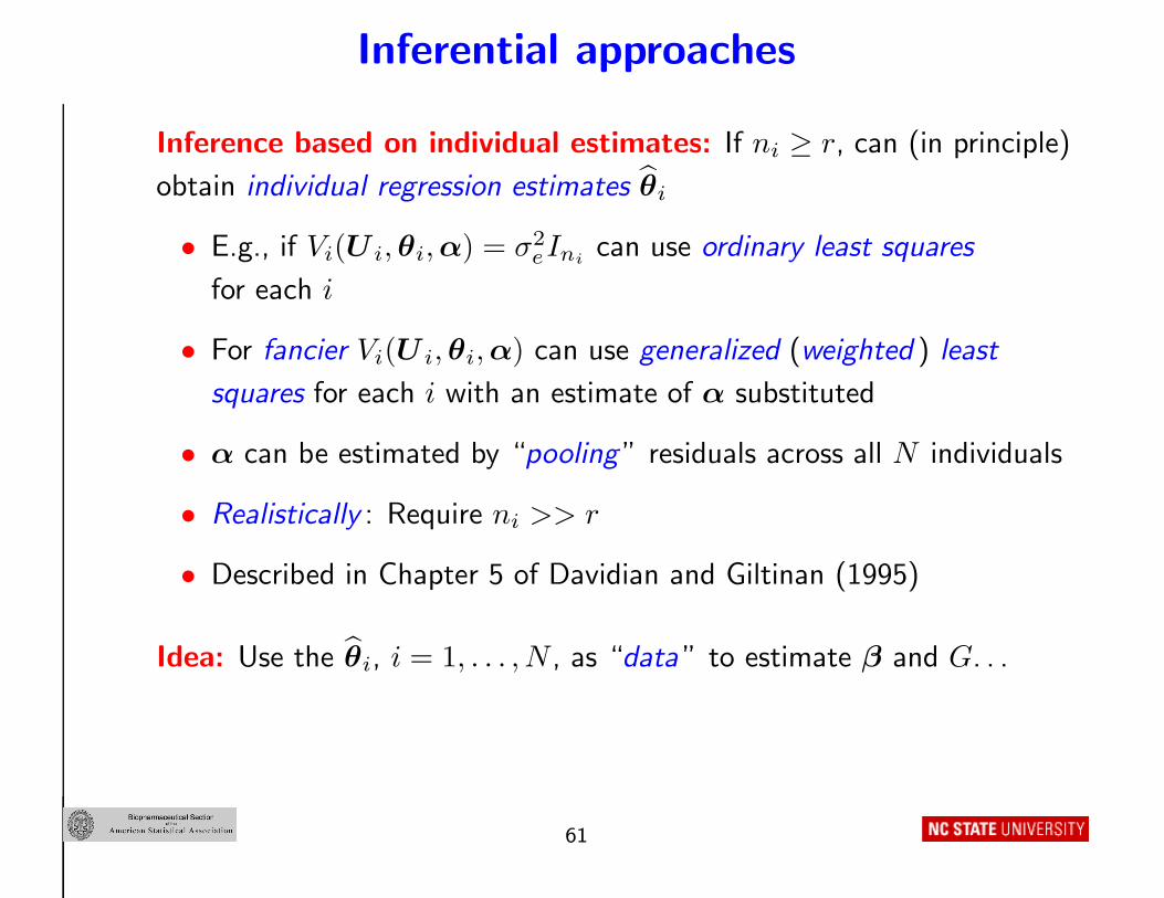
Inference based on individual estimates: If ni ≥ r, can (in principle)
obtain individual regression estimates θi
• E.g., if Vi(U i, θi, α) = σ2eIni
can use ordinary least squares
for each i
• For fancier Vi(U i, θi, α) can use generalized (weighted ) least
squares for each i with an estimate of α substituted
• α can be estimated by “pooling ” residuals across all N individuals
• Realistically : Require ni >> r
• Described in Chapter 5 of Davidian and Giltinan (1995)
Idea: Use the θi, i = 1, . . . , N , as “data ” to estimate β and G. . .
61
Inferential approaches
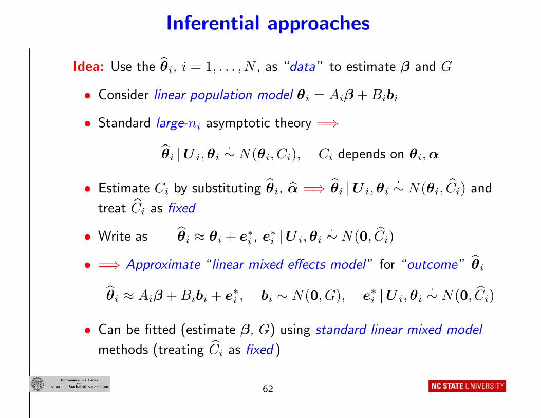
Idea: Use the θi, i = 1, . . . , N , as “data ” to estimate β and G
• Consider linear population model θi = Aiβ + Bibi
• Standard large-ni asymptotic theory =⇒
θi |U i, θi·∼ N(θi, Ci), Ci depends on θi, α
• Estimate Ci by substituting θi, α =⇒ θi |U i, θi·∼ N(θi, Ci) and
treat Ci as fixed
• Write as θi ≈ θi + e∗
i , e∗
i |U i, θi·∼ N(0, Ci)
• =⇒ Approximate “linear mixed effects model ” for “outcome ” θi
θi ≈ Aiβ + Bibi + e∗
i , bi ∼ N(0, G), e∗
i |U i, θi·∼ N(0, Ci)
• Can be fitted (estimate β, G) using standard linear mixed model
methods (treating Ci as fixed )
62
Inferential approaches
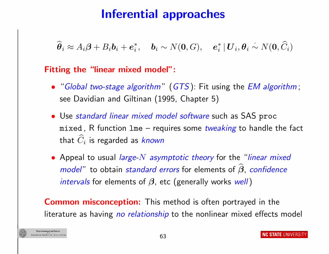
θi ≈ Aiβ + Bibi + e∗
i , bi ∼ N(0, G), e∗
i |U i, θi·∼ N(0, Ci)
Fitting the “linear mixed model”:
• “Global two-stage algorithm ” (GTS ): Fit using the EM algorithm ;
see Davidian and Giltinan (1995, Chapter 5)
• Use standard linear mixed model software such as SAS proc
mixed , R function lme – requires some tweaking to handle the fact
that Ci is regarded as known
• Appeal to usual large-N asymptotic theory for the “linear mixed
model ” to obtain standard errors for elements of β, confidence
intervals for elements of β, etc (generally works well )
Common misconception: This method is often portrayed in the
literature as having no relationship to the nonlinear mixed effects model
63
Inferential approaches
How does this approximate the integrals? Not readily apparent
• May view the θi as approximate “sufficient statistics ” for the θi
• Change of variables in the integrals and replace fi(yi |xi, bi; γ) by
the (normal) density f(θi |U i, θi; α) corresponding to the
asymptotic approximation
Remarks:
• When all ni are sufficiently large to justify the asymptotic
approximation (e.g., intensive PK studies), I like this method!
• Easy to explain to collaborators
• Gives similar answers to other analytical approximation methods
(coming up)
• Drawback : No standard software (although see my website for
R/SAS code)
64

Inferential approaches
In many settings: “Rich ” individual data not available for all i
(e.g., population PK studies); i.e., ni “not large ” for some or all i
• Approximate the integrals more directly by approximating
fi(yi |xi; γ, G)
Write model with normality assumptions at both stages:
Y i = mi(Xi, β, bi) + V1/2i (Xi, β, bi, α) ǫi, bi ∼ N(0, G)
• V1/2i (ni × ni) such that V
1/2i (V
1/2i )′ = Vi
• ǫi |Xi, bi ∼ N(0, Ini) (ni × 1)
• First-order Taylor series about bi = b∗
i “close” to bi, ignoring
cross-product (bi − b∗
i )ǫi as negligible =⇒
Y i ≈ mi(Xi, β, b∗i )−Zi(Xi, β, b∗i )b∗
i +Zi(Xi, β, b∗i )bi+V1/2i (Xi, β, b∗i , α) ǫi
Zi(Xi, β, b∗i ) = ∂/∂bi{mi(Xi, β, bi)}|bi = b∗
i
65
Inferential approaches
Y i ≈ mi(Xi, β, b∗i )−Zi(Xi, β, b∗i )b∗
i +Zi(Xi, β, b∗i )bi+V1/2i (Xi, β, b∗i , α) ǫi
“First-order” method: Take b∗
i = 0 (mean of bi)
• =⇒ Distribution of Y i given Xi approximately normal with
E(Y i |Xi) ≈ mi(Xi, β,0),
Cov(Y i |Xi) ≈ Zi(Xi, β,0) GZ ′
i(Xi, β,0) + Vi(Xi, β,0, α)
• =⇒ Approximate fi(yi |xi; γ, G) by a normal density with these
moments, so that ℓ(γ, G) is in a closed form
• =⇒ Estimate (β, α, G) by maximum likelihood – because integrals
are eliminated, is a direct optimization (but still very messy. . . )
• First proposed by Beal and Sheiner in early 1980s in the context of
population PK
66
Inferential approaches
“First-order” method: Software
• fo method in the Fortran package nonmem (widely used by PKists)
• SAS proc nlmixed using the method=firo option
Alternative implementation: View as an approximate
“population-averaged ” model for mean and covariance
E(Y i |Xi) ≈ mi(Xi, β,0),
Cov(Y i |Xi) ≈ Zi(Xi, β,0) GZ ′
i(Xi, β,0) + Vi(Xi, β,0, α)
• =⇒ Estimate (β, α, G) by solving a set of generalized estimating
equations (GEEs; specifically, “GEE-1 ”)
• Is a different method from maximum likelihood (“GEE-2 ”)
• Software : SAS macro nlinmix with expand=zero
67
Inferential approaches
Problem: These approximate moments are clearly poor approximations
to the true moments
• In particular, poor approximation to E(Y i |Xi) =⇒ biased
estimators for β
“First-order conditional methods”: Use a “better ” approximation
• Take b∗i “closer ”to bi
• Natural choice: bi = mode of the posterior density
f(bi |yi, xi; γ, G) =fi(yi |xi, bi; γ) f(bi; G)
fi(yi |xi; γ, G)
• =⇒ Approximate moments
E(Y i |Xi) ≈ mi(Xi, β, bi) − Zi(Xi, β, bi)bi
Cov(Y i |Xi) ≈ Zi(Xi, β, bi) GZ ′
i(Xi, β, bi) + Vi(Xi, β, bi, α)
68

Inferential approaches
Fitting algorithms: Iterate between
(i) Update bi, i = 1, . . . , N , by maximizing the posterior density (or
approximation to it) with γ and G substituted and held fixed
(ii) Hold the bi fixed and update estimation of γ and G by either
(a) Maximizing the approximate normal log-likelihood based on
treating Y i given Xi as normal with these moments, OR
(b) Solving a corresponding set of GEEs
• Usually “converges ” (although no guarantee )
Software:
• nonmem with foce option implements (ii)(a)
• R function nlme, SAS macro nlinmix with expand=blup option
implement (ii)(b)
69
Inferential approaches
Standard errors, etc: For both “first-order ” approximations
• Pretend that the approximate moments are exact and use the usual
large-N asymptotic theory for maximum likelihood or GEEs
• Provides reliable inferences in problems where N is reasonably large
and the magnitude of among-individual variation is not huge
My experience:
• Even without the integration, these are nasty computational
problems , and good starting values for the parameters are required
(may have to try several sets of starting values).
• The “first-order ” approximation is too crude and should be avoided
in general (although can be a good way to get reasonable starting
values for other methods)
• The “first-order conditional ” methods often work well, are
numerically well-behaved , and yield reliable inferences
70
Inferential approaches
ℓ(γ, G) = log
{N∏
i=1
∫fi(yi |xi, bi; γ) f(bi; G) dbi
}
Numerical approximation methods: Approximate the integrals using
deterministic or stochastic numerical integration techniques
(q-dimensional numerical integration ) and maximize the log-likelihood
• Issue : For each iteration of the likelihood optimization algorithm,
must approximate N q-dimensional integrals
• Infeasible until recently: Numerical integration embedded repeatedly
in an optimization routine is computationally intensive
• Gets worse with larger q (the “curse of dimensionality ”)
71
Inferential approaches
Deterministic techniques:
• Normality of bi =⇒ Gauss-Hermite quadrature
• Quadrature rule : Approximate an integral by a suitable weighted
average of the integrand evaluated at a q-dimensional grid of values
=⇒ accuracy increases with more grid points, but so does
computational burden
• Adaptive Gaussian quadrature : “Center ” and “scale ” the grid
about bi =⇒ can greatly reduce the number of grid points needed
Software: SAS proc nlmixed
• Adaptive Gaussian quadrature : The default
• Gaussian quadrature : method=gauss noad
72
Inferential approaches
ℓ(γ, G) = log
{N∏
i=1
∫fi(yi |xi, bi; γ) f(bi; G) dbi
}
Stochastic techniques:
• “Brute force ” Monte Carlo integration: Represent integral for i by
B−1B∑
b=1
fi(yi |xi, b(b); γ),
b(b) are draws from N(0, G) (at the current estimates of γ, G)
• Can require very large B for acceptable accuracy (inefficient )
• Importance sampling : Replace this by a suitably weighted version
that is more efficient
Software: SAS proc nlmixed implements importance sampling
(method=isamp)
73
Inferential approaches
My experience with SAS proc nlmixed:
• Good starting values are essential (may have to try many sets) –
starting values are required for all of β, G, α
• Could obtain starting values from an analytical approximation
method
• Practically speaking, quadrature is infeasible for q > 2 almost always
with the mechanism-based nonlinear models in PK and other
applications
74
Inferential approaches
Other methods: Maximize the log-likelihood via an EM algorithm
• For nonlinear mixed models , the conditional expectation in the
E-step is not available in a closed form
• Monte Carlo EM algorithm : Approximate the E-step by ordinary
Monte Carlo integration
• Stochastic approximation EM algorithm : Approximate the E-step by
Monte Carlo simulation and stochastic approximation
• Software : MONOLIX (http://www.monolix.org/)
75

Inferential approaches
Bayesian inference : Natural approach to hierarchical models
Big picture: In the Bayesian paradigm
• View β, α, G, and bi, i = 1, . . . , N , as random parameters (on
equal footing) with prior distributions (priors for bi, i = 1, . . . , N ,
are N(0, G))
• Bayesian inference on β and G is based on their posterior
distributions
• The posterior distributions involve high-dimensional integration and
cannot be derived analytically . . .
• . . . but samples from the posterior distributions can be obtained via
Markov chain Monte Carlo (MCMC)
76

Inferential approaches
Bayesian hierarchy:
• Stage 1 – Individual-level model : Assume normality
E(Y i |Xi, bi) = E(Y i |U i, θi) = mi(U i, θi) = mi(Xi, β, bi),
Cov(Y i |Xi, bi) = Cov(Y i |U i, θi) = Vi(U i, θi, α) = Vi(Xi, β, bi, α)
• Stage 2 – Population model : θi = d(Ai, β, bi), bi ∼ N(0, G)
• Stage 3 – Hyperprior : (β, α, G) ∼ f(β, α, G) = f(β)f(α)g(G)
• Joint posterior density
f(γ, G, b |y, x) =
∏Ni=1 fi(yi |xi, bi; γ) f(bi; G)f(β, α, G)
f(y |x);
denominator is numerator integrated wrt (γ, G, bi, i = 1, . . . , N)
• E.g., posterior for β, f(β |y, x): Integrate out α, G, bi, i = 1, . . . , N
77
Inferential approaches
Estimator for β: Mode of posterior
• Uncertainty measured by spread of f(β |y, x)
• Similarly for α, G, and bi, i = 1, . . . , N
Implementation: By simulation via MCMC
• Samples from the full conditional distributions (eventually) behave
like samples from the posterior distributions
• The mode and measures of uncertainty may be calculated
empirically from these samples
• Issue : Sampling from some of the full conditionals is not entirely
straightforward because of nonlinearity of m in θi and hence bi
• =⇒ “All-purpose ” software not available in general, but has been
implemented for popular m in add-ons to WinBUGS (e.g., PKBugs)
78
Inferential approaches
Experience:
• With weak hyperpriors and “good ” data, inferences are very similar
to those based on maximum likelihood and first-order conditional
methods
• Convergence of the chain must be monitored carefully; “false
convergence ” can happen
• Advantage of Bayesian framework : Natural mechanism to
incorporate known constraints and prior scientific knowledge
79
Inferential approaches
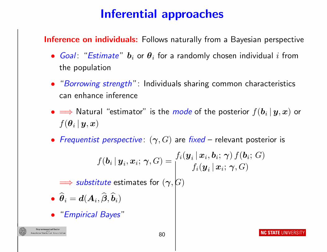
Inference on individuals: Follows naturally from a Bayesian perspective
• Goal : “Estimate ” bi or θi for a randomly chosen individual i from
the population
• “Borrowing strength ”: Individuals sharing common characteristics
can enhance inference
• =⇒ Natural “estimator” is the mode of the posterior f(bi |y, x) or
f(θi |y, x)
• Frequentist perspective : (γ, G) are fixed – relevant posterior is
f(bi |yi, xi; γ, G) =fi(yi |xi, bi; γ) f(bi; G)
fi(yi |xi; γ, G)
=⇒ substitute estimates for (γ, G)
• θi = d(Ai, β, bi)
• “Empirical Bayes ”
80

Inferential approaches
Selecting the population model d: Everything so far is predicated on
a fixed d(Ai, β, bi)
• A key objective in many analyses (e.g., population PK) is to identify
an appropriate d(Ai, β, bi)
• Must identify elements of Ai to include in each component of
d(Ai, β, bi) and the functional form of each component
• Likelihood inference : Use nested hypothesis tests or information
criteria (AIC, BIC, etc)
• Challenging when Ai is high-dimensional. . .
• . . . Need a way of selecting among large number of variables and
functional forms in each component (still an open problem. . . )
81
Inferential approaches
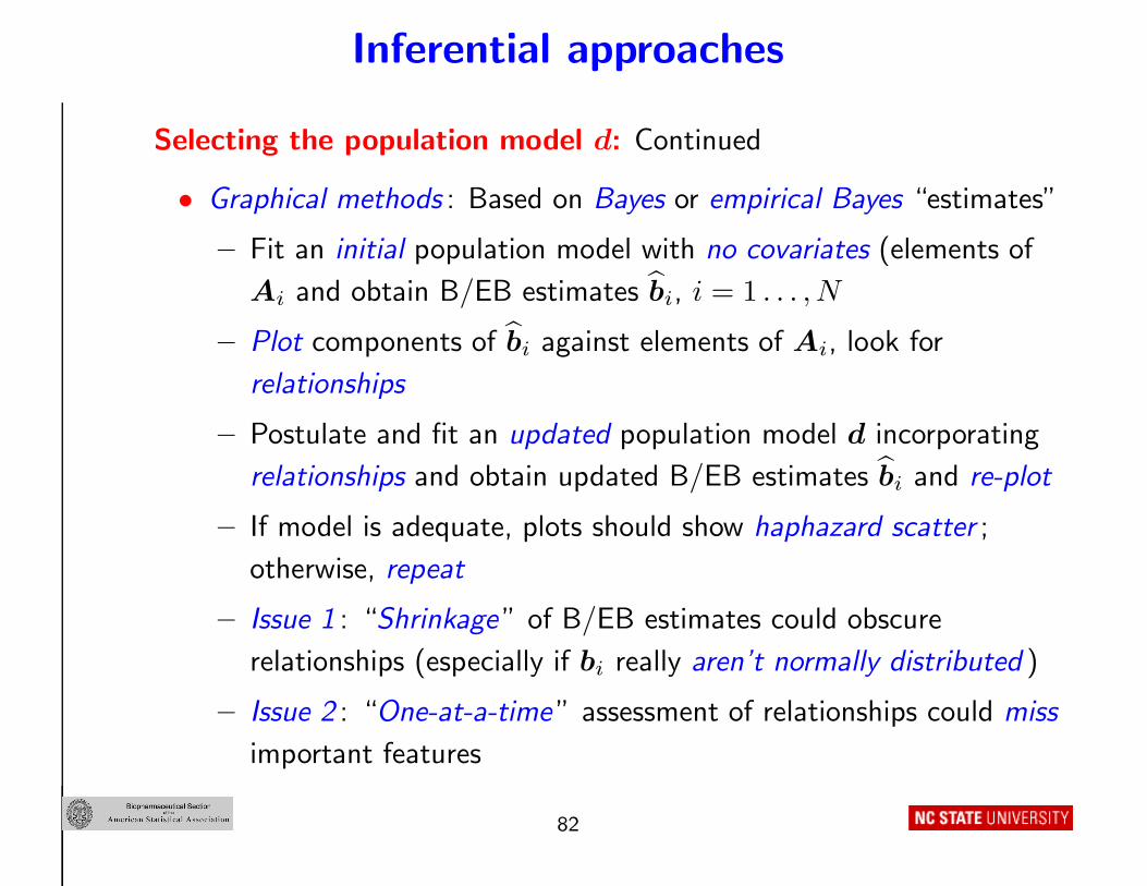
Selecting the population model d: Continued
• Graphical methods : Based on Bayes or empirical Bayes “estimates”
– Fit an initial population model with no covariates (elements of
Ai and obtain B/EB estimates bi, i = 1 . . . , N
– Plot components of bi against elements of Ai, look for
relationships
– Postulate and fit an updated population model d incorporating
relationships and obtain updated B/EB estimates bi and re-plot
– If model is adequate, plots should show haphazard scatter ;
otherwise, repeat
– Issue 1 : “Shrinkage ” of B/EB estimates could obscure
relationships (especially if bi really aren’t normally distributed )
– Issue 2 : “One-at-a-time ” assessment of relationships could miss
important features
82
Inferential approaches
Normality of bi: The assumption bi ∼ N(0, G) is standard in mixed
effects model analysis; however
• Is it always realistic ?
• Unmeasured binary among-individual covariate systematically
associated with θi =⇒ bi has bimodal distribution
• Or a normal distribution may just not be the best model!
(heavy tails , skewness. . . )
• Consequences ?
Relaxing the normality assumption: Represent the density of bi by a
flexible form
• Estimate the density along with the model parameters
• =⇒ Insight into possible omitted covariates
83
Applications
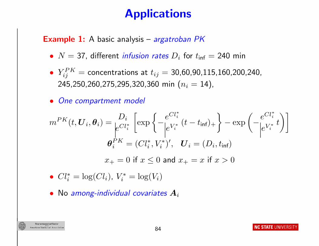
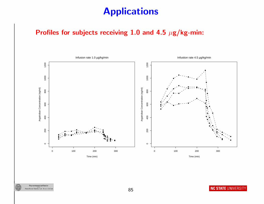
Example 1: A basic analysis – argatroban PK
• N = 37, different infusion rates Di for tinf = 240 min
• Y PKij = concentrations at tij = 30,60,90,115,160,200,240,
245,250,260,275,295,320,360 min (ni = 14),
• One compartment model
mPK(t, U i, θi) =Di
eCl∗i
[exp
{−eCl∗i
eV ∗
i
(t − tinf)+
}− exp
(−eCl∗i
eV ∗
i
t
)]
θPKi = (Cl∗i , V ∗
i )′, U i = (Di, tinf)
x+ = 0 if x ≤ 0 and x+ = x if x > 0
• Cl∗i = log(Cli), V ∗
i = log(Vi)
• No among-individual covariates Ai
84
Applications
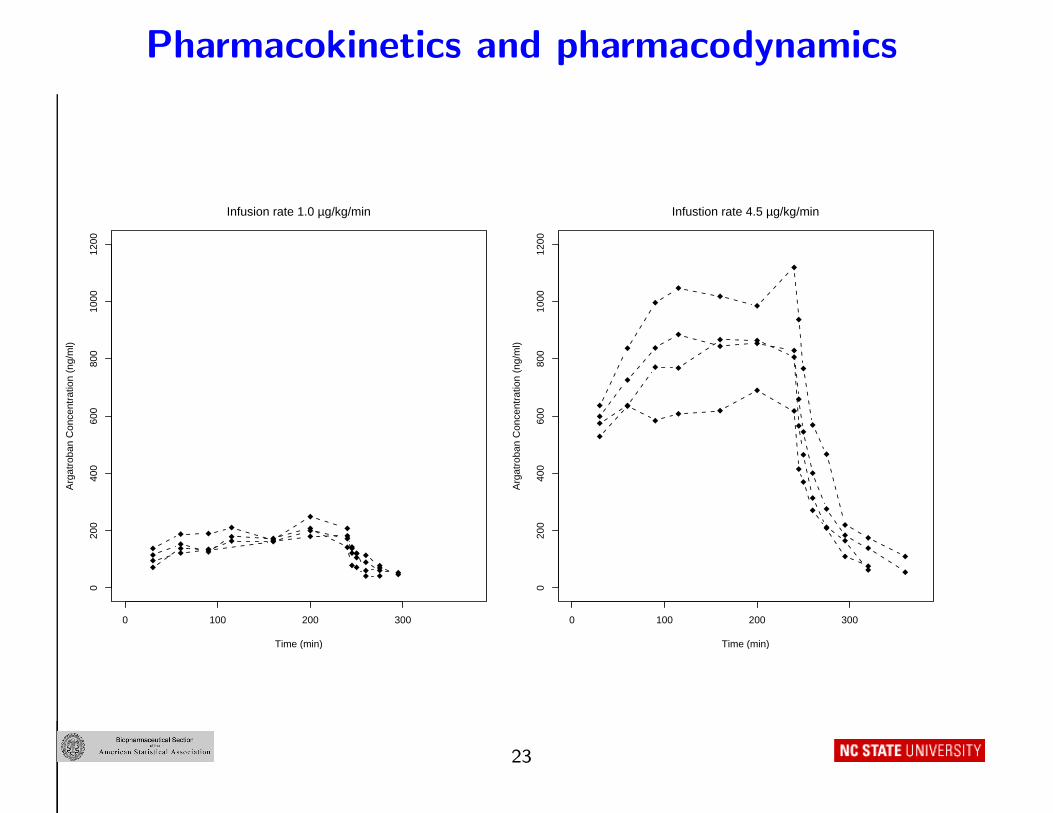
Profiles for subjects receiving 1.0 and 4.5 µg/kg-min:
0 100 200 300
020
040
060
080
010
0012
00
Time (min)
Arg
atro
ban
Con
cent
ratio
n (n
g/m
l)
Infusion rate 1.0 µg/kg/min
0 100 200 300
020
040
060
080
010
0012
00
Time (min)
Arg
atro
ban
Con
cent
ratio
n (n
g/m
l)
Infustion rate 4.5 µg/kg/min
85
Applications
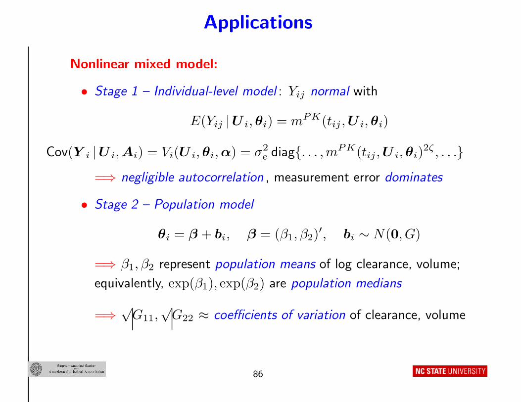
Nonlinear mixed model:
• Stage 1 – Individual-level model : Yij normal with
E(Yij |U i, θi) = mPK(tij , U i, θi)
Cov(Y i |U i, Ai) = Vi(U i, θi, α) = σ2e diag{. . . , mPK(tij , U i, θi)
2ζ , . . .}=⇒ negligible autocorrelation , measurement error dominates
• Stage 2 – Population model
θi = β + bi, β = (β1, β2)′, bi ∼ N(0, G)
=⇒ β1, β2 represent population means of log clearance, volume;
equivalently, exp(β1), exp(β2) are population medians
=⇒√
G11,√
G22 ≈ coefficients of variation of clearance, volume
86
Applications
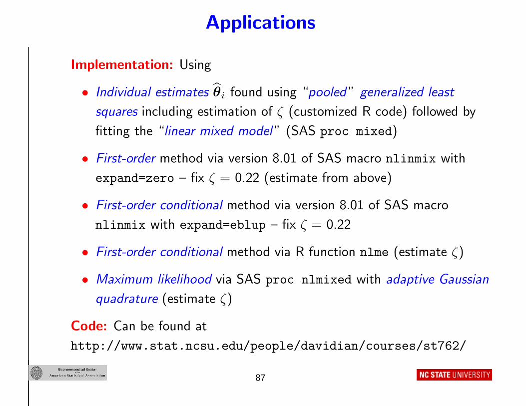
Implementation: Using
• Individual estimates θi found using “pooled ” generalized least
squares including estimation of ζ (customized R code) followed by
fitting the “linear mixed model ” (SAS proc mixed)
• First-order method via version 8.01 of SAS macro nlinmix with
expand=zero – fix ζ = 0.22 (estimate from above)
• First-order conditional method via version 8.01 of SAS macro
nlinmix with expand=eblup – fix ζ = 0.22
• First-order conditional method via R function nlme (estimate ζ)
• Maximum likelihood via SAS proc nlmixed with adaptive Gaussian
quadrature (estimate ζ)
Code: Can be found at
http://www.stat.ncsu.edu/people/davidian/courses/st762/
87
Applications
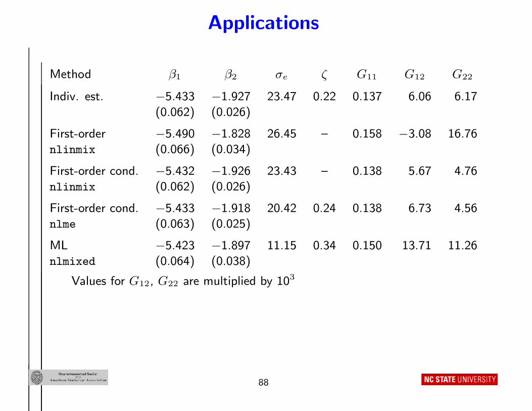
Method β1 β2 σe ζ G11 G12 G22
Indiv. est. −5.433 −1.927 23.47 0.22 0.137 6.06 6.17
(0.062) (0.026)
First-order −5.490 −1.828 26.45 – 0.158 −3.08 16.76nlinmix (0.066) (0.034)
First-order cond. −5.432 −1.926 23.43 – 0.138 5.67 4.76nlinmix (0.062) (0.026)
First-order cond. −5.433 −1.918 20.42 0.24 0.138 6.73 4.56
nlme (0.063) (0.025)
ML −5.423 −1.897 11.15 0.34 0.150 13.71 11.26
nlmixed (0.064) (0.038)
Values for G12, G22 are multiplied by 103
88

Applications
Interpretation: Based on the individual estimates results
• Concentrations measured in ng/ml = 1000 µg/ml
• Median argatroban clearance ≈ 4.4 µg/ml/kg
(≈ exp(−5.43) × 1000)
• Median argatroban volume ≈ 145.1 ml/kg =⇒ ≈ 10 liters for
a 70 kg subject
• Assuming Cli, Vi approximately lognormal
– G11 ≈√
0.14× 100 ≈ 37% coefficient of variation for clearance
– G22 ≈√
0.00617× 100 ≈ 8% CV for volume
89

Applications
Individual inference: Individual estimate (dashed) and empirical Bayes
estimate (solid)
0 100 200 300
020
040
060
080
010
0012
00
Time (minutes)
Arg
atro
ban
Con
cent
ratio
n (n
g/m
l)
0 100 200 3000
200
400
600
800
1000
1200
Time (minutes)
Arg
atro
ban
Con
cent
ratio
n (n
g/m
l)
90
Applications
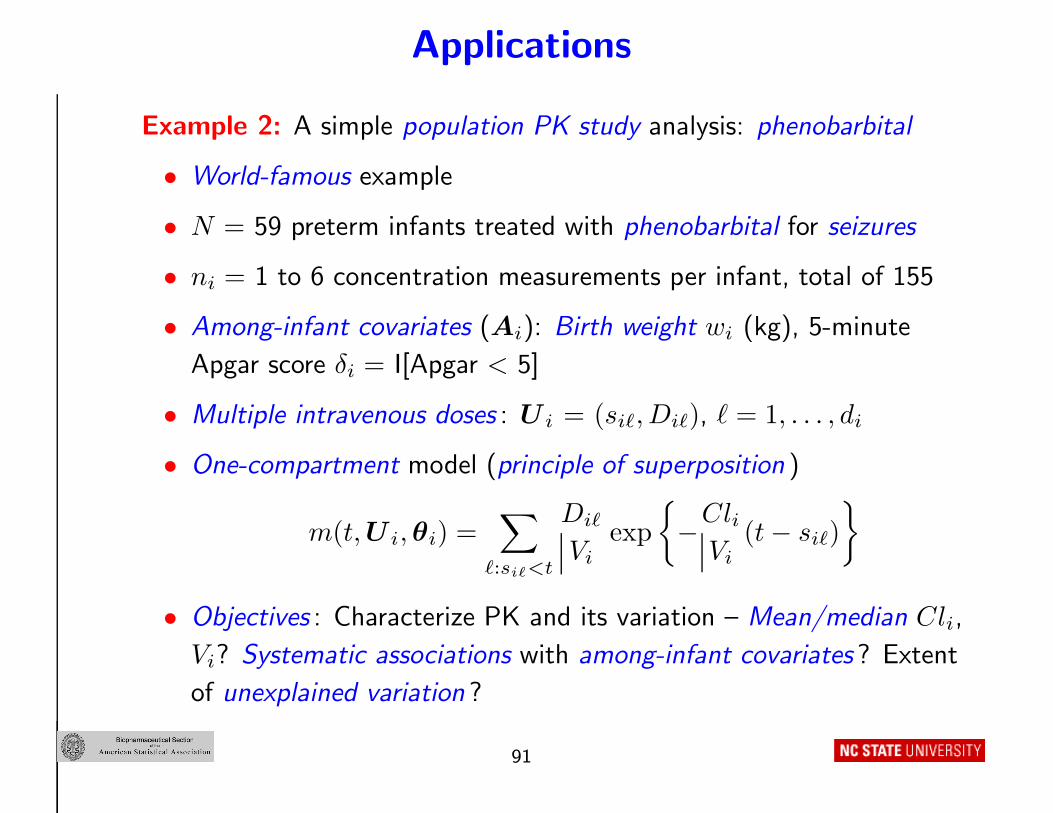
Example 2: A simple population PK study analysis: phenobarbital
• World-famous example
• N = 59 preterm infants treated with phenobarbital for seizures
• ni = 1 to 6 concentration measurements per infant, total of 155
• Among-infant covariates (Ai): Birth weight wi (kg), 5-minute
Apgar score δi = I[Apgar < 5]
• Multiple intravenous doses : U i = (siℓ, Diℓ), ℓ = 1, . . . , di
• One-compartment model (principle of superposition )
m(t, U i, θi) =∑
ℓ:siℓ<t
Diℓ
Viexp
{−Cli
Vi(t − siℓ)
}
• Objectives : Characterize PK and its variation – Mean/median Cli,
Vi? Systematic associations with among-infant covariates ? Extent
of unexplained variation ?
91
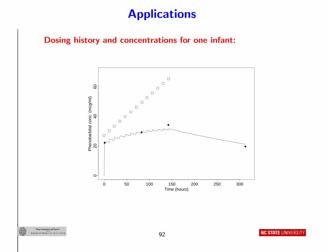
Applications
Dosing history and concentrations for one infant:
Time (hours)
Phe
noba
rbita
l con
c. (
mcg
/ml)
0 50 100 150 200 250 300
020
4060
92

Applications
Nonlinear mixed model:
• Stage 1 – Individual-level model
E(Yij |U i, θi) = m(tij , U i, θi), Cov(Y i |U i, Ai) = Vi(U i, θi, α) = σ2e Ini
=⇒ negligible autocorrelation , measurement error dominates and
has constant variance
• Stage 2 – Population model
– Without among-infant covariates Ai
log Cli = β1 + bi1, log Vi = β2 + bi2
– With among-infant covariates Ai
log Cli = β1 + β3wi + bi1, log Vi = β2 + β4wi + β5δi + bi2
93
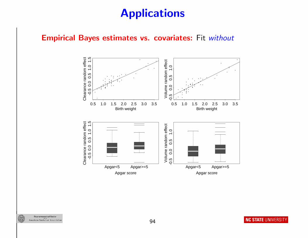
Applications
Empirical Bayes estimates vs. covariates: Fit without
..
.
.
.
.. . ..
.
... ...
.
. ..
.
..
.
.
.
.
.
.
.
.
....
..
.
..
.
.
.
..
.
.
....
. ..
.
.
..
Birth weight
Cle
aran
ce r
ando
m e
ffect
0.5 1.0 1.5 2.0 2.5 3.0 3.5
-0.5
0.0
0.5
1.0
1.5
. ..
.
.
.. .
.
...
..
..
... .
..
..
.
.
.
.
.
.
.
.
...
...
..
.
.
.
.
..
.
.
.
..
.
. ..
.
.
..
Birth weight
Vol
ume
rand
om e
ffect
0.5 1.0 1.5 2.0 2.5 3.0 3.5
-0.5
0.0
0.5
1.0
-0.5
0.0
0.5
1.0
1.5
Apgar<5 Apgar>=5
Apgar score
Cle
aran
ce r
ando
m e
ffect
-0.5
0.0
0.5
1.0
Apgar<5 Apgar>=5
Apgar score
Vol
ume
rand
om e
ffect
94
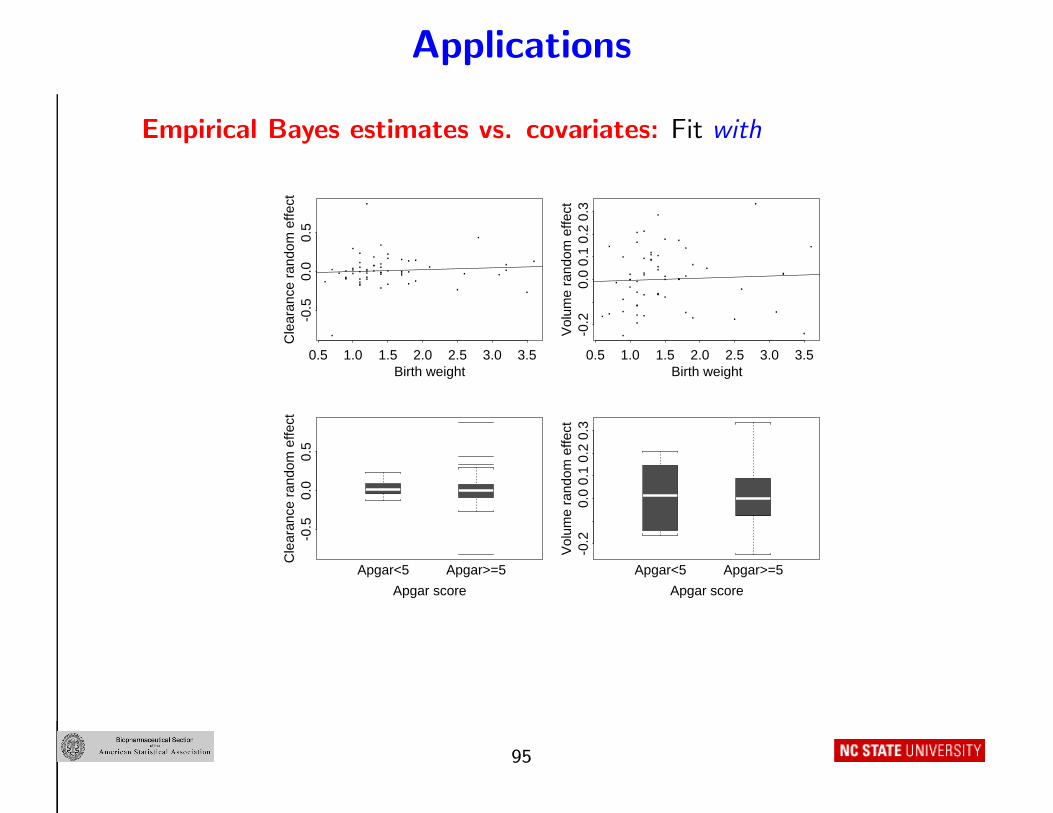
Applications
Empirical Bayes estimates vs. covariates: Fit with
..
.
.
.
..
..
.
.
... ...
.
. . .. ...
..
...
..
...
... .. .
.
..
. . .
.
..
.. ..
.
...
.
Birth weight
Cle
aran
ce r
ando
m e
ffect
0.5 1.0 1.5 2.0 2.5 3.0 3.5
-0.5
0.0
0.5
.
.
.
.
.
.
.
.
.
.
.
.
.
.
..
...
...
.
.
.
..
..
.
.
.
..
.
..
..
. .
.
.
.
. . .
.
.
.
.
.
.
.
.
.
.
..
Birth weight
Vol
ume
rand
om e
ffect
0.5 1.0 1.5 2.0 2.5 3.0 3.5
-0.2
0.0
0.1
0.2
0.3
-0.5
0.0
0.5
Apgar<5 Apgar>=5
Apgar score
Cle
aran
ce r
ando
m e
ffect
-0.2
0.0
0.1
0.2
0.3
Apgar<5 Apgar>=5
Apgar score
Vol
ume
rand
om e
ffect
95
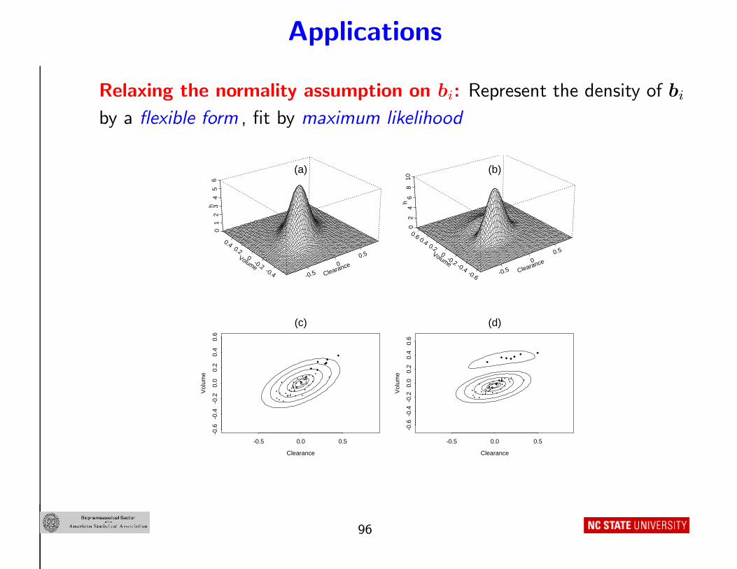
Applications
Relaxing the normality assumption on bi: Represent the density of bi
by a flexible form , fit by maximum likelihood
-0.5 0
0.5
Clearance-0.4
-0.2
0
0.2
0.4
Volume
01
23
45
6h
(a)
Clearance
Vol
ume
-0.5 0.0 0.5
-0.6
-0.4
-0.2
0.0
0.2
0.4
0.6
..
..
.. .
...
.
.
. ....
.... .
.
.
.
..
.. ..
.
...
.. ....
.
.
..... .
.
.
..
.
...
..
(c)
-0.5 0
0.5
Clearance
-0.6
-0.4
-0.2
00.2
0.4
0.6
Volume
02
46
810
h
(b)
Clearance
Vol
ume
-0.5 0.0 0.5
-0.6
-0.4
-0.2
0.0
0.2
0.4
0.6
..
..
.
. ...
.
.
.. .
.........
.
.
..
.. ..
.
..... ..
..
.
...... .
.
.
...
.
....
(d)
96

Extensions
Multivariate outcome: More than one type of outcome measured
longitudinally on each individual
• Objectives: Understand the relationships between the outcome
trajectories and the processes underlying them
• Key example : Pharmacokinetics/pharmacodynamics (PK/PD) as in
argatroban
97

Extensions
Required: A joint model for PK and PD
• Data :
– Y PKij at times tPK
ij (PK concentrations)
– Y PDij at times tPD
ij (PD aPTT responses)
• PK model with θPKi = (Cl∗i , V ∗
i )′, U i = (Di, tinf)
mPK(t, U i, θPKi ) =
Di
eCl∗i
[exp
{eCl∗i
eV ∗
i
(t − tinf)+
}− exp
(−eCl∗i
eV ∗
i
t
)]
• PD model with θPDi = (E∗
0i, E∗
max,i, EC∗
50,i)′
mPD(conc, θPDi ) = eE∗
0i +eE∗
max,i − eE∗
0i
1 + eEC∗
50,i/conc
98
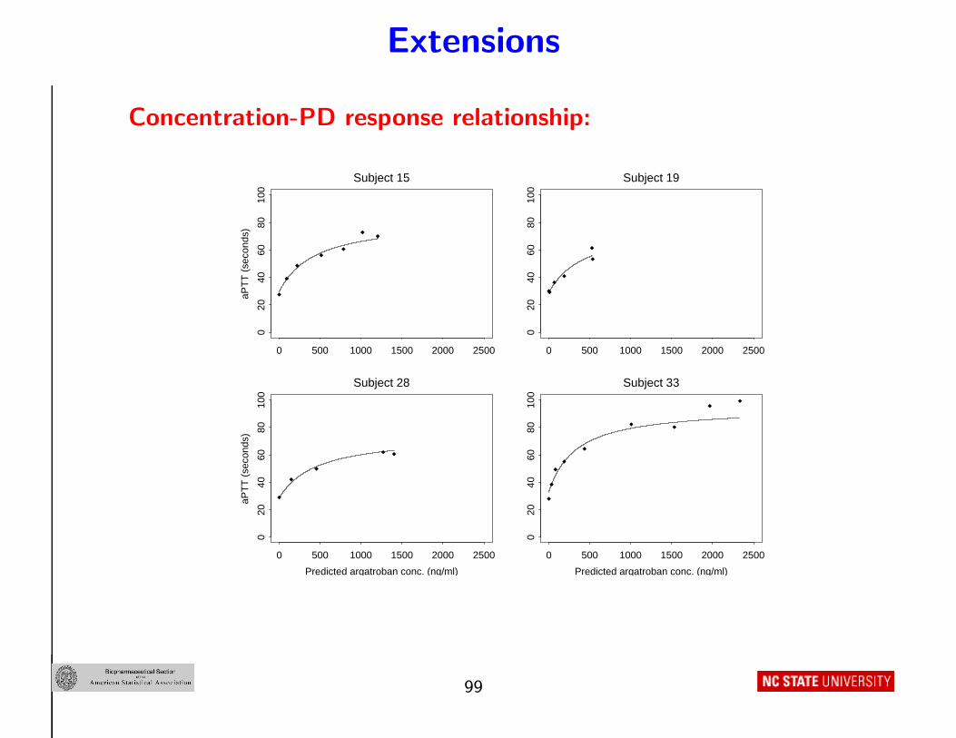
Extensions
Concentration-PD response relationship:
aPT
T (
seco
nds)
0 500 1000 1500 2000 2500
020
4060
8010
0
Subject 15
0 500 1000 1500 2000 2500
020
4060
8010
0
Subject 19
Predicted argatroban conc. (ng/ml)
aPT
T (
seco
nds)
0 500 1000 1500 2000 2500
020
4060
8010
0
Subject 28
Predicted argatroban conc. (ng/ml)
0 500 1000 1500 2000 2500
020
4060
8010
0
Subject 33
99
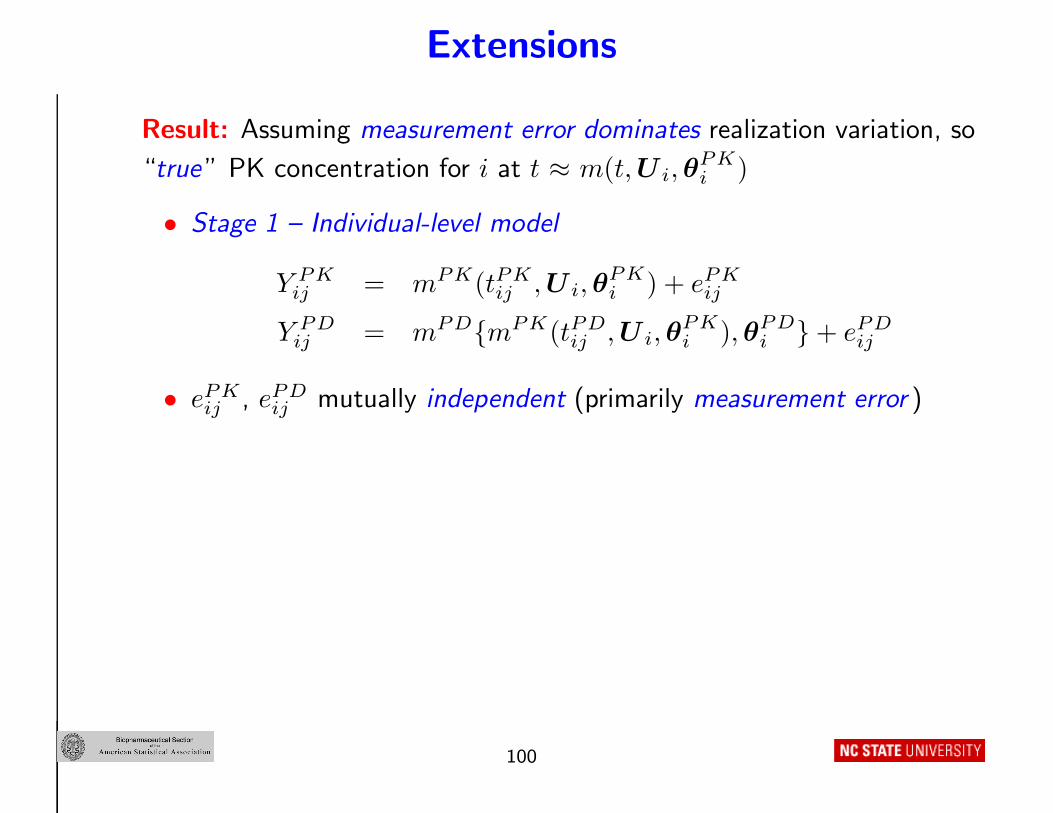
Extensions
Result: Assuming measurement error dominates realization variation, so
“true ” PK concentration for i at t ≈ m(t, U i, θPKi )
• Stage 1 – Individual-level model
Y PKij = mPK(tPK
ij , U i, θPKi ) + ePK
ij
Y PDij = mPD{mPK(tPD
ij , U i, θPKi ), θPD
i } + ePDij
• ePKij , ePD
ij mutually independent (primarily measurement error )
100

Extensions
Full model: Combined outcomes Y i = (Y PK′
i , Y PD′
i )′
θi = (θPK′
i , θPD′
i )′ = (Cl∗i , V ∗
i , E∗
0i, E∗
max,i, EC∗
50i)′
• Stage 1 – Individual-level model
E(Y PKij |U i, θi) = mPK(tPK
ij , U i, θPKi )
E(Y PDij |U i, θi) = mPD{mPK(tPD
ij , U i, θPKi ), θPD
i }
Cov(Y i|U i, θi) = block diag{V PKi (U i, θi, α
PK), V PDi (U i, θi, α
PD)}
V PKi (U i, θi, α
PK) = σ2e,PKdiag{. . . , mPK(tPK
ij , U i, θPKi )2ζPK
, . . .}
V PDi (U i, θi, α
PD) = σ2e,PDdiag
[. . . , mPD{mPK(tPD
ij , U i, θPKi ), θPD
i }2ζP D
, . . .]
• Stage 2 – Population model
θi = β + bi, β = (β1, . . . , β5)′, bi ∼ N(0, G)
101
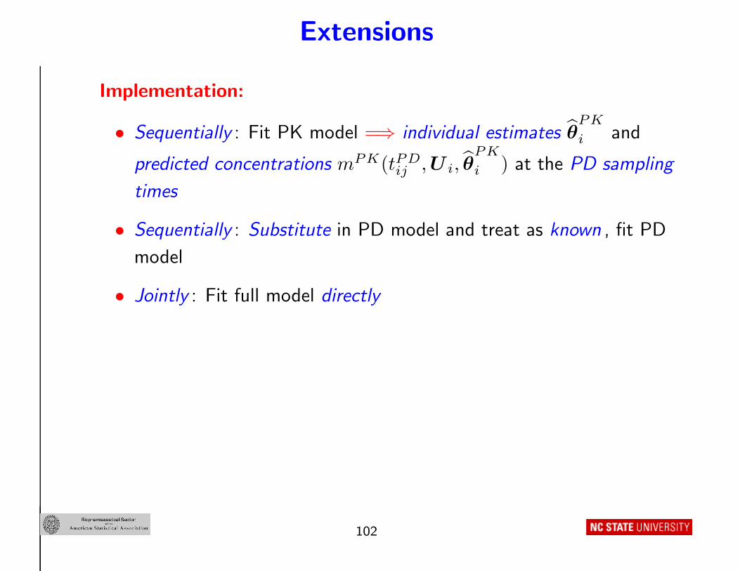
Extensions
Implementation:
• Sequentially : Fit PK model =⇒ individual estimates θPK
i and
predicted concentrations mPK(tPDij , U i, θ
PK
i ) at the PD sampling
times
• Sequentially : Substitute in PD model and treat as known , fit PD
model
• Jointly : Fit full model directly
102
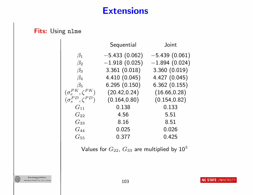
Extensions
Fits: Using nlme
Sequential Joint
β1 −5.433 (0.062) −5.439 (0.061)
β2 −1.918 (0.025) −1.894 (0.024)β3 3.361 (0.018) 3.360 (0.019)
β4 4.410 (0.045) 4.427 (0.045)β5 6.295 (0.150) 6.362 (0.155)
(σP K
e , ζP K) (20.42,0.24) (16.66,0.28)(σP D
e , ζP D) (0.164,0.80) (0.154,0.82)
G11 0.138 0.133G22 4.56 5.51
G33 8.16 8.51G44 0.025 0.026
G55 0.377 0.425
Values for G22, G33 are multiplied by 103
103
Extensions
Time-dependent among-individual covariates: Among-individual
covariates change over time within an individual
• In principle , one could write θij for each tij ; however . . .
• Key issue : Does this make scientific sense ?
• PK : Do pharmacokinetic processes vary within an individual?
Example: Quinidine study
• Creatinine clearance, α1-acid glycoprotein concentration, etc,
change over dosing intervals
• How to incorporate dependence of Cli, Vi on α1-acid glycoprotein
concentration?
104

Extensions
Data for a representative subject:
time conc. dose age weight creat. glyco.(hours) (mg/L) (mg) (years) (kg) (ml/min) (mg/dl)
0.00 – 166 75 108 > 50 696.00 – 166 75 108 > 50 69
11.00 – 166 75 108 > 50 6917.00 – 166 75 108 > 50 6923.00 – 166 75 108 > 50 6927.67 0.7 – 75 108 > 50 6929.00 – 166 75 108 > 50 9435.00 – 166 75 108 > 50 9441.00 – 166 75 108 > 50 9447.00 – 166 75 108 > 50 9453.00 – 166 75 108 > 50 9465.00 – 166 75 108 > 50 9471.00 – 166 75 108 > 50 9477.00 0.4 – 75 108 > 50 94
161.00 – 166 75 108 > 50 88168.75 0.6 – 75 108 > 50 88
height=72 inches, Caucasian, smoker, no ethanol abuse, no CHF
105
Extensions
Population model: Standard approach in PK
• For subject i: α1-acid glycoprotein concentration likely measured
intermittently at times 0, 29, 161 hours and assumed constant over
the intervals (0,29), (29,77), (161,·) hours
• For intervals Ik, k = 1, . . . , a (a = 3 here), Aik = among-individual
covariates for tij ∈ Ik =⇒ e.g., linear model
θij = Aikβ + bi
• This population model assumes “within subject inter-interval
variation ” entirely “explained ” by changes in covariate values
• Alternatively : Nested random effects
θij = Aikβ + bi + bik, bi, bik independent
106
Extensions
Multi-level models: More generally
• Nesting : E.g., outcomes Yikj , j = 1, . . . , nik, on several trees
(k = 1, . . . , vi) within each of several plots (i = 1, . . . , N)
θik = Aikβ + bi + bik, bi, bik independent
Missing/mismeasured covariates: Ai, U i, tij
Censored outcome: E.g., due to an assay quantification limit
Semiparametric models: Allow m(t, U i, θi) to depend on an
unspecified function g(t, θi)
• Flexibility , model misspecification
Clinical trial simulation: “Virtual ” subjects simulated from a nonlinear
mixed effects model for PK/PD/disease progression linked to a clinical
end-point
107
Discussion
Summary:
• The nonlinear mixed effects model is now a standard statistical
framework in many areas of application
• Is appropriate when scientific interest focuses on within-individual
mechanisms/processes that can be represented by parameters in a
nonlinear (often theoretical ) model for individual time course
• Free and commercial software is available, but implementation is
still complicated
• Specification of models and assumptions, particularly the population
model , is somewhat an art-form
• Current challenge : High-dimensional Ai (e.g., genomic information)
• Still plenty of methodological research to do
108

Discussion
See the references on slide 3 for an extensive bibliography
109