Bayesian Statistics Made SimpleAllen B. DowneyOlin College

sites.google.com/site/simplebayes

Follow along at home

sites.google.com/site/simplebayes

The plan

From Bayes's Theorem to Bayesian inference.

A computational framework.

Work on example problems.

Goals

By the end, you should be ready to:

● Work on similar problems.● Learn more on your own.

Think Bayes

This tutorial is based on my book,Think BayesBayesian Statistics in Python

Published by O'Reilly Mediaand available under aCreative Commons license fromthinkbayes.com

Probability

p(A): the probability that A occurs.

p(A|B): the probability that A occurs, given that B has occurred.

p(A and B) = p(A) p(B|A)

Bayes's Theorem

By definition of conjoint probability:p(A and B) = p(A) p(B|A) = (1)p(B and A) = p(B) p(A|B)

Equate the right hand sidesp(B) p(A|B) = p(A) p(B|A) (2)

Divide by p(B) and ...

Bayes's Theorem

Bayes's Theorem

One way to think about it:

Bayes's Theorem is an algorithm to get from p(B|A) to p(A|B).

Useful if p(B|A), p(A) and p(B) are easier than p(A|B).

OR ...

Diachronic interpretation

H: HypothesisD: Data

Given p(H), the probability of the hypothesis before you saw the data.

Find p(H|D), the probability of the hypothesis after you saw the data.

A cookie problem

Suppose there are two bowls of cookies.Bowl #1 has 10 chocolate and 30 vanilla.Bowl #2 has 20 of each.

Fred picks a bowl at random, and then picks a cookie at random. The cookie turns out to be vanilla.

What is the probability that Fred picked from Bowl #1?

from Wikipedia

Cookie problem

H: Hypothesis that cookie came from Bowl 1.D: Cookie is vanilla.

Given p(H), the probability of the hypothesis before you saw the data.

Find p(H|D), the probability of the hypothesis after you saw the data.

Diachronic interpretation

p(H|D) = p(H) p(D|H) / p(D)

p(H): prior

p(D|H): conditional likelihood of the data

p(D): total likelihood of the data

Diachronic interpretation

p(H|D) = p(H) p(D|H) / p(D)

p(H): prior = 1/2

p(D|H): conditional likelihood of the data = 3/4

p(D): total likelihood of the data = 5/8

Diachronic interpretation

p(H|D) = (1/2)(3/4) / (5/8) = 3/5

p(H): prior = 1/2

p(D|H): conditional likelihood of the data = 3/4

p(D): total likelihood of the data = 5/8

A little intuition

p(H): prior = 50%

p(H|D): posterior = 60%

Vanilla cookie was more likely under H.

Slightly increases our degree of belief in H.

Computation

Pmf represents a Probability Mass Function

Maps from possible values to probabilities.

Diagram by yuml.me

Install test

How many of you got install_test.py running?

Don't try to fix it now!

Instead...

Partner up

● If you don't have a working environment, find a neighbor who does.

● Even if you do, try pair programming!● Take a minute to introduce yourself.● Questions? Ask your partner first (please).

Icebreaker

What was your first computer?

What was your first programming language?

What is the longest time you have spent finding a stupid bug?

Start your engines

1. You cloned BayesMadeSimple, right?2. cd into that directory.3. Start the Python interpreter.

$ python

>>> from thinkbayes import Pmf

Or IPython

1. cd into BayesMadeSimple.2. Start IPython.3. Create a new notebook.

$ ipython notebook --matplotlib inline

from thinkbayes import Pmf

Pmf

from thinkbayes import Pmf

# make an empty Pmfd6 = Pmf()

# outcomes of a six-sided diefor x in [1,2,3,4,5,6]: d6.Set(x, 1)

Pmf

d6.Print()

d6.Normalize()

d6.Print()

d6.Random()

Style

I know what you're thinking.

The Bayesian framework

1) Build a Pmf that maps from each hypothesis to a prior probability, p(H).

2) Multiply each prior probability by the likelihood of the data, p(D|H).

3) Normalize, which divides through by the total likelihood, p(D).

Prior

pmf = Pmf()pmf.Set('Bowl 1', 0.5)pmf.Set('Bowl 2', 0.5)

Update

p(Vanilla | Bowl 1) = 30/40p(Vanilla | Bowl 2) = 20/40

pmf.Mult('Bowl 1', 0.75)pmf.Mult('Bowl 2', 0.5)

Normalize

pmf.Normalize()0.625 # return value is p(D)

print pmf.Prob('Bowl 1')0.6

Exercise

What if we select another cookie, and it’s chocolate?

The posterior (after the first cookie) becomes the prior (before the second cookie).

Exercise

What if we select another cookie, and it’s chocolate?

pmf.Mult('Bowl 1', 0.25)pmf.Mult('Bowl 2', 0.5)pmf.Normalize()pmf.Print()Bowl 1 0.43Bowl 2 0.573

Summary

Bayes's Theorem,Cookie problem,Pmf class.

The dice problem

I have a box of dice that contains a 4-sided die, a 6-sided die, an 8-sided die, a 12-sided die and a 20-sided die.

Suppose I select a die from the box at random, roll it, and get a 6. What is the probability that I rolled each die?

Hypothesis suites

A suite is a mutually exclusive and collectively exhaustive set of hypotheses.

Represented by a Suite that maps hypothesis → probability.

Suite

class Suite(Pmf):

"Represents a suite of hypotheses and

their probabilities."

def __init__(self, hypos):

"Initializes the distribution."

for hypo in hypos:

self.Set(hypo, 1)

self.Normalize()

Suite

def Update(self, data):

"Updates the suite based on data."

for hypo in self.Values(): like = self.Likelihood(data, hypo) self.Mult(hypo, like)

self.Normalize()

self.Likelihood?

Suite

Likelihood is an abstract method.

Child classes inherit Update,provide Likelihood.

Likelihood

Outcome: 6● What is the likelihood of this outcome on a

six-sided die?● On a ten-sided die?● On a four-sided die?

What is the likelihood of getting n on an m-sided die?

Likelihood# hypo is the number of sides on the die# data is the outcome

class Dice(Suite):

def Likelihood(self, data, hypo): # write this method!

Write your solution in dice.py

Likelihood# hypo is the number of sides on the die# data is the outcome

class Dice(Suite):

def Likelihood(self, data, hypo): if hypo < data: return 0 else: return 1.0/hypo

Dice

# start with equal priorssuite = Dice([4, 6, 8, 12, 20])

# update with the datasuite.Update(6)

suite.Print()

Dice

Posterior distribution:4 0.06 0.398 0.3012 0.1920 0.12

More data? No problem...

Dice

for roll in [8, 7, 7, 5, 4]: suite.Update(roll)

suite.Print()

Dice

Posterior distribution:4 0.06 0.08 0.9212 0.08020 0.0038

Summary

Dice problem,Likelihood function,Suite class.

Recess!

http

://ks

dciti

zens

.org

/wp-

cont

ent/u

ploa

ds/2

010/

09/re

cess

_tim

e.jp

g

Trains

The trainspotting problem:● You believe that a freight carrier operates

between 100 and 1000 locomotives with consecutive serial numbers.

● You spot locomotive #321.● How many locomotives does the carrier

operate?

Modify train.py to compute your answer.

Trains

● If there are m trains, what is the chance of spotting train #n?

● What does the posterior distribution look like?

● How would you summarize it?

Train

print suite.Mean()print suite.MaximumLikelihood()print suite.CredibleInterval(90)

Trains

● What if we spot more trains?

● Why did we do this example?

Trains

● Practice using the Bayesian framework, and figuring out Likelihood().

● Example that uses sparse data.

● It’s a non-trivial, real problem.

Tanks

The German tank problem.http://en.wikipedia.org/wiki/German_tank_problem

Good time for questions

A Euro problem

"When spun on edge 250 times, a Belgian one-euro coin came up heads 140 times and tails 110. 'It looks very suspicious to me,' said Barry Blight, a statistics lecturer at the London School of Economics. 'If the coin were unbiased, the chance of getting a result as extreme as that would be less than 7%.' "

From "The Guardian" quoted by MacKay, Information Theory, Inference, and Learning Algorithms.

A Euro problem

MacKay asks, "But do these data give evidence that the coin is biased rather than fair?"

Assume that the coin has probability x of landing heads.

(Forget that x is a probability; just think of it as a physical characteristic.)

A Euro problem

Estimation: Based on the data (140 heads, 110 tails), what is x?

Hypothesis testing: What is the probability that the coin is fair?

Euro

We can use the Suite template again.

We just have to figure out the likelihood function.

Likelihood# hypo is the prob of heads (1-100)# data is a string, either 'H' or 'T'

class Euro(Suite):

def Likelihood(self, data, hypo): # one more, please!

Modify euro.py to compute your answer.

Likelihood# hypo is the prob of heads (1-100)# data is a string, either 'H' or 'T'

class Euro(Suite):

def Likelihood(self, data, hypo): x = hypo / 100.0 if data == 'H': return x else: return 1-x

Prior

What do we believe about x before seeing the data?

Start with something simple; we'll come back and review.

Uniform prior: any value of x between 0% and 100% is equally likely.

Prior

suite = Euro(range(0, 101))

Update

Suppose we spin the coin once and get heads.

suite.Update('H')

What does the posterior distribution look like?

Hint: what is p(x=0% | D)?

Update

Suppose we spin the coin again, and get heads again.

suite.Update('H')

What does the posterior distribution look like?

Update

Suppose we spin the coin again, and get tails.

suite.Update('T')

What does the posterior distribution look like?

Hint: what's p(x=100% | D)?

Update

After 10 spins, 7 heads and 3 tails:

for outcome in 'HHHHHHHTTT': suite.Update(outcome)

Update

And finally, after 140 heads and 110 tails:

evidence = 'H' * 140 + 'T' * 110for outcome in evidence: suite.Update(outcome)

Posterior

● Now what?● How do we summarize the information in the

posterior Suite?

Posterior

Given the posterior distribution, what is the probability that x is 50%?

suite.Prob(50)

And the answer is... 0.021

Hmm. Maybe that's not the right question.

Posterior

How about the most likely value of x?

pmf.MaximumLikelihood()

And the answer is 56%.

Posterior

Or the expected value?

suite.Mean()

And the answer is 55.95%.

Posterior

Credible interval?

suite.CredibleInterval(90)

Posterior

The 5th percentile is 51.The 95th percentile is 61.

These values form a 90% credible interval.

So can we say: "There's a 90% chance that x is between 51 and 61?"

Frequentist response

Thank you smbc-comics.com

Bayesian response

Yes, x is a random variable,Yes, (51, 61) is a 90% credible interval,Yes, x has a 90% chance of being in it.

Pro: Bayesian stats are amenable to decision analysis.

Con: The prior is subjective.

The prior is subjective

Remember the prior?

We chose it pretty arbitrarily, and reasonable people might disagree.

Is x as likely to be 1% as 50%?

Given what we know about coins, I doubt it.

Prior

How should we capture background knowledge about coins?

Try a triangle prior.

Posterior

What do you think the posterior distributions look like?

I was going to put an image here, but then I Googled "posterior". Never mind.

Swamp the prior

With enough data, reasonable people converge.

But if any p(Hi) = 0, no data will change that.

Swamp the prior

Priors can be arbitrarily low, but avoid 0.

See wikipedia.org/wiki/Cromwell's_rule

"I beseech you, in the bowels of Christ, think it possible that you may be mistaken."

Summary of estimation

1. Form a suite of hypotheses, Hi.

2. Choose prior distribution, p(Hi).

3. Compute likelihoods, p(D|Hi).

4. Turn off brain.

5. Compute posteriors, p(Hi|D).

Recess!

http

://im

ages

2.w

ikia

.noc

ooki

e.ne

t/__c

b201

2011

6013

507/

rece

ss/im

ages

/4/4

c/R

eces

s_P

ic_f

or_t

he_I

nter

net.p

ng

Hypothesis testing

Remember the original question:

"But do these data give evidence that the coin is biased rather than fair?"

What does it mean to say that data give evidence for (or against) a hypothesis?

Hypothesis testing

D is evidence in favor of H ifp(H|D) > p(H)which is true ifp(D|H) > p(D|~H)or equivalently ifp(D|H) / p(D|~H) > 1

Hypothesis testing

This term

p(D|H) / p(D|~H)

is called the likelihood ratio, or Bayes factor.

It measures the strength of the evidence.

Hypothesis testing

F: hypothesis that the coin is fairB: hypothesis that the coin is biased

p(D|F) is easy.p(D|B) is hard because B is underspecified.

Bogosity

Tempting: we got 140 heads out of 250 spins, so B is the hypothesis that x = 140/250.

But,1. Doesn't seem right to use the data twice.2. By this process, almost any data would be

evidence in favor of B.

We need some rules

1. You have to choose your hypothesis before you see the data.

2. You can choose a suite of hypotheses, but in that case we average over the suite.

Likelihood

def AverageLikelihood(suite, data):

total = 0

for hypo, prob in suite.Items():

like = suite.Likelihood(data, hypo)

total += prob * like

return total

Hypothesis testing

F: hypothesis that x = 50%.

B: hypothesis that x is not 50%, but might be any other value with equal probability.

Prior

fair = Euro() fair.Set(50, 1)

Prior

bias = Euro() for x in range(0, 101): if x != 50: bias.Set(x, 1) bias.Normalize()

Bayes factor

data = 140, 110

like_fair = AverageLikelihood(fair, data)

like_bias = AverageLikelihood(bias, data)

ratio = like_bias / like_fair

Hypothesis testing

Read euro2.py.

Notice the new representation of the data, and corresponding Likelihood function.

Run it and interpret the results.

Hypothesis testing

And the answer is:

p(D|B) = 2.6 · 10-76

p(D|F) = 5.5 · 10-76

Likelihood ratio is about 0.47.

So this dataset is evidence against B.

Fair comparison?

● Modify the code that builds bias; try out a different definition of B and run again.

bias = Euro() for x in range(0, 49): bias.Set(x, x) for x in range(51, 101): bias.Set(x, 100-x) bias.Normalize()

Conclusion

● The Bayes factor depends on the definition of B.

● Depending on what “biased” means, the data might be evidence for or against B.

● The evidence is weak either way (between 0.5 and 2).

Summary

Euro problem,Bayesian estimation,Bayesian hypothesis testing.

Recess!

http

://ks

dciti

zens

.org

/wp-

cont

ent/u

ploa

ds/2

010/

09/re

cess

_tim

e.jp

g

Word problem for geeks

ALICE: What did you get on the math SAT?

BOB: 760

ALICE: Oh, well I got a 780. I guess that means I'm smarter than you.

NARRATOR: Really? What is the probability that Alice is smarter than Bob?

Assume, define, quantify

Assume: each person has some probability, x, of answering a random SAT question correctly.

Define: "Alice is smarter than Bob" means xa > xb.

How can we quantify Prob { xa > xb } ?

Be Bayesian

Treat x as a random quantity.

Start with a prior distribution.

Update it.

Compare posterior distributions.

Prior?Distribution of raw scores.

Likelihood

def Likelihood(self, data, hypo): x = hypo score = data raw = self.exam.Reverse(score)

yes, no = raw, self.exam.max_score - raw like = x**yes * (1-x)**no return like

Posterior

PmfProbGreater

def PmfProbGreater(pmf1, pmf2):

    """Returns the prob that a value from pmf1

is greater than a value from pmf2."""

PmfProbGreater

def PmfProbGreater(pmf1, pmf2):

    """Returns the prob that a value from pmf1

is greater than a value from pmf2."""

Iterate through all pairs of values.

Check whether the value from pmf1 is greater.

Add up total probability of successful pairs.

PmfProbGreater

def PmfProbGreater(pmf1, pmf2):

    

    for x1, p1 in pmf1.Items():

        for x2, p2 in pmf2.Items():

# FILL THIS IN!

           

PmfProbGreater

def PmfProbGreater(pmf1, pmf2):

    

    total = 0.0

    for x1, p1 in pmf1.Items():

        for x2, p2 in pmf2.Items():

            if x1 > x2:

                total += p1 * p2

    return total

And the answer is...

Alice: 780

Bob: 760

Probability that Alice is "smarter": 61%

Why this example?

Posterior distribution is often the input to the next step in an analysis.

Real world problems start (and end!) with modeling.

Modeling

● This result is based on the simplification that all SAT questions are equally difficult.

● An alternative (in the book) is based on item response theory.

Modeling

● For most real world problems, there are several reasonable models.

● The best choice depends on your goals.● Modeling errors often dominate.

Modeling

Therefore:

● Don't mistake the map for the territory.

● Don't sweat approximations smaller than

modeling errors.

● Iterate.

Recess!

http

://im

ages

2.w

ikia

.noc

ooki

e.ne

t/__c

b201

2011

6013

507/

rece

ss/im

ages

/4/4

c/R

eces

s_P

ic_f

or_t

he_I

nter

net.p

ng

Case study

Problem: students sign up to participate in a community service project. Some fraction, q, of the students who sign up actually participate, and of those some fraction, r, report back.

Given a sample of students who sign up and the number who report back, we can estimate the product q*r, but don't learn about q and r separately.

Case study

If we can get a smaller sample of students where we know who participated and who reported, we can use that to improve the estimates of q and r.

And we can use that to compute the posterior distribution of the number of students who participated.

volunteer.py

probs = numpy.linspace(0, 1, 101)

hypos = [] for q in probs: for r in probs: hypos.append((q, r))

suite = Volunteer(hypos)

volunteer.py

# students who signed up and reported

data = 140, 50 suite.Update(data)

# students who signed up, participated,

# and reported data = 5, 3, 1 suite.Update(data)

volunteer.py

class Volunteer(thinkbayes.Suite):

def Likelihood(self, data, hypo): if len(data) == 2: return self.Likelihood1(data, hypo) elif len(data) == 3: return self.Likelihood2(data, hypo) else: raise ValueError()

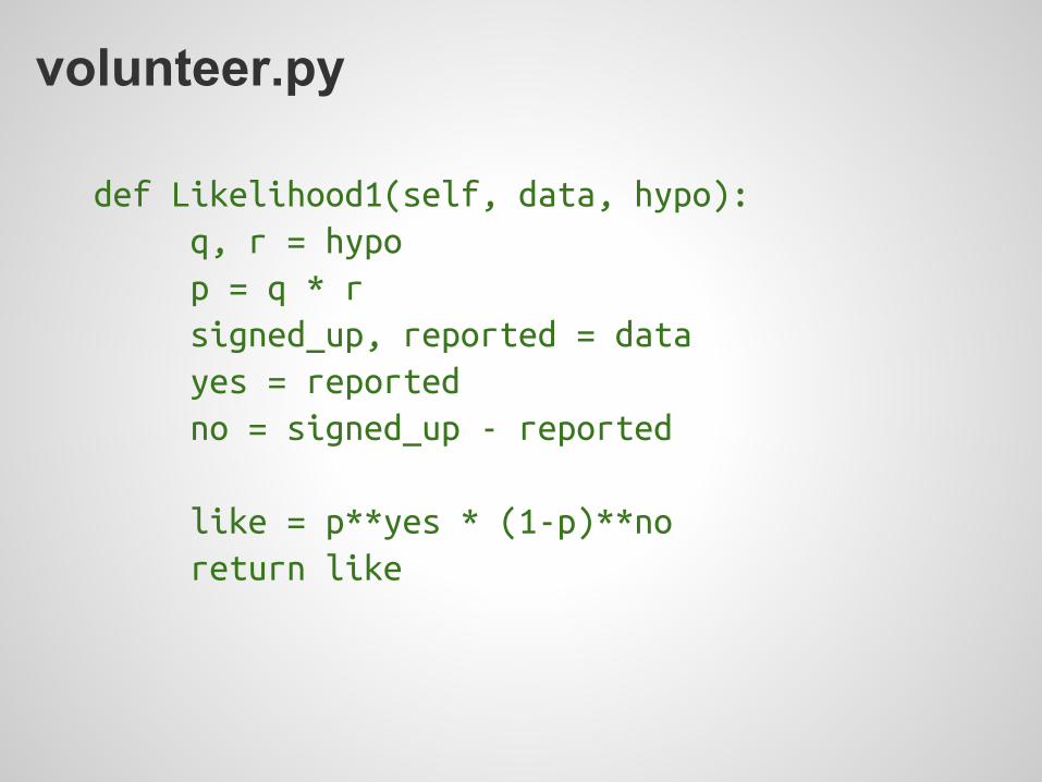
volunteer.py

def Likelihood1(self, data, hypo): q, r = hypo p = q * r signed_up, reported = data yes = reported no = signed_up - reported

like = p**yes * (1-p)**no return like

volunteer.py

def Likelihood2(self, data, hypo): q, r = hypo signed_up, participated, reported = data yes = participated no = signed_up - participated like1 = q**yes * (1-q)**no

yes = reported no = participated - reported like2 = r**yes * (1-r)**no

return like1 * like2

volunteer.py

def MarginalDistribution(suite, index):

pmf = thinkbayes.Pmf() for t, prob in suite.Items(): pmf.Incr(t[index], prob) return pmf

Summary

● The Bayesian approach is a divide and conquer strategy.

● You write Likelihood().● Bayes does the rest.

Think Bayes

This tutorial is based on my book,Think BayesBayesian Statistics Made Simple

Published by O'Reilly Mediaand available under aCreative Commons license fromthinkbayes.com

Case studies

● Euro ● SAT ● Red line ● Price is Right● Boston Bruins ● Paintball● Variability hypothesis● Kidney tumor growth● Geiger counter● Unseen species

Think Stats

You might also likeThink Stats, 2nd editionExploratory Data Analysis

Published by O'Reilly Mediaand available under aCreative Commons license fromthinkstats2.com

More reading

MacKay, Information Theory, Inference, and Learning Algorithms

Free PDF.

More reading

Davidson-Pilon,Bayesian Methodsfor Hackers

On Github.

More reading (not free)

Howson and Urbach, Scientific Reasoning: The Bayesian Approach

Sivia, Data Analysis: A Bayesian Tutorial

Gelman et al, Bayesian Data Analysis

Where does this fit?

Usual approach:● Analytic distributions.● Math.● Multidimensional integrals.● Numerical methods (MCMC).

Where does this fit?

Problem:● Hard to get started.● Hard to develop solutions incrementally.● Hard to develop understanding.

My theory

● Start with non-analytic distributions.● Use background information to choose

meaningful priors.● Start with brute-force solutions.● If the results are good enough and fast

enough, stop.● Otherwise, optimize (where analysis is one

kind of optimization).● Use your reference implementation for

regression testing.

Need help?

I am always looking for interesting projects.● Sabbatical June 2015 to August 2016.

Data Science at Olin

● January to May 2015.● 30 students, 15 projects.● External collaborators with data and

questions.● Exploratory data analysis and visualization.● Focus on health, medicine, and fitness.

sites.google.com/site/datascience15/

datakind.org