mth709u/mthm042 bayesian statistics

1

MTH709U/MTHM042Bayesian Statistics

Lawrence PettitQueen Mary, Spring 2012

Contents

1 Introduction 71.1 Bayes theorem . . . . . . . . . . . . . . . . . . . . . . . . . . . 71.2 The Likelihood Principle . . . . . . . . . . . . . . . . . . . . . . 91.3 Other criticisms of classical methods . . . . . . . . . . . . . . . . 11

2 The Bayesian Paradigm 152.1 Sufficiency and the Exponential Family . . . . . . . . . . . . . . 152.2 Families closed under sampling . . . . . . . . . . . . . . . . . . . 172.3 Non-informative priors . . . . . . . . . . . . . . . . . . . . . . . 25

2.3.1 Jeffreys’ prior . . . . . . . . . . . . . . . . . . . . . . . . 282.4 Two sample problems . . . . . . . . . . . . . . . . . . . . . . . . 292.5 Predictive distributions . . . . . . . . . . . . . . . . . . . . . . . 322.6 Constraints on parameters . . . . . . . . . . . . . . . . . . . . . . 332.7 Estimation and Tests . . . . . . . . . . . . . . . . . . . . . . . . 35

2.7.1 Point estimation . . . . . . . . . . . . . . . . . . . . . . 352.7.2 Interval estimation . . . . . . . . . . . . . . . . . . . . . 362.7.3 Hypothesis testing . . . . . . . . . . . . . . . . . . . . . 38

2.8 Nuisance parameters . . . . . . . . . . . . . . . . . . . . . . . . 41

3 Linear Models 433.1 Introduction . . . . . . . . . . . . . . . . . . . . . . . . . . . . . 433.2 Uniform priors . . . . . . . . . . . . . . . . . . . . . . . . . . . 443.3 Normal priors . . . . . . . . . . . . . . . . . . . . . . . . . . . . 463.4 Three stage model . . . . . . . . . . . . . . . . . . . . . . . . . . 503.5 Exchangeability . . . . . . . . . . . . . . . . . . . . . . . . . . . 533.6 Unknown variances . . . . . . . . . . . . . . . . . . . . . . . . . 55

4 Approximate methods 574.1 Numerical Integration . . . . . . . . . . . . . . . . . . . . . . . . 574.2 Asymptotic normality of the posterior distribution . . . . . . . . . 594.3 Laplace’s method for evaluating integrals . . . . . . . . . . . . . 62

3

4 CONTENTS

4.4 Gibbs sampling . . . . . . . . . . . . . . . . . . . . . . . . . . . 654.4.1 Introduction . . . . . . . . . . . . . . . . . . . . . . . . . 654.4.2 The basic algorithm . . . . . . . . . . . . . . . . . . . . . 664.4.3 Constraints on parameters . . . . . . . . . . . . . . . . . 694.4.4 Missing data problems . . . . . . . . . . . . . . . . . . . 694.4.5 Discussion . . . . . . . . . . . . . . . . . . . . . . . . . 70

5 Criticisms and Answers 71

Preface

The majority of statistics courses use the ‘classical’ approach which is based onthe idea that probability represents a long run limiting frequency. Bayesian statis-tics is based on subjective probability, the idea that a probability represents a per-sonal degree of belief in an event which is conditional on the knowledge of theperson concerned. Different people have different knowledge and it is not surpris-ing that they should have different probabilities for the same event. Objectivityarises when enough subjectivists agree, for example on the simple events of pick-ing cards or throwing dice.

In this course we shall introduce you to Bayesian statistics. The most usefulrequirement is to have an open mind; to be willing to look at an unfamiliar way ofdoing statistics.

These notes are largely self-contained but it is good to read other accounts ofBayesian statistics as well. The principal books for this course are:

• Bayesian Statistics: An Introduction (2nd or 3rd ed.) by P M Lee, EdwardArnold.

• Bayesian Statistical Inference by G Iversen, Sage. (Although this is just abrief introduction to the subject written for Social Scientists).

In addition parts of the following are useful:

• Bayesian Inference for Statistical Analysis by G E P Box and G C Tiao,Wiley Classics Series.

• Bayesian Data Analysis by A Gelman, J B Carlin, H S Stern and D B Rubin,Chapman and Hall.

• Probability and Statistics from a Bayesian viewpoint (Vol 2) by D V Lind-ley, Cambridge University Press.

Good luck with the course.

5

6 CONTENTS

Chapter 1

Introduction

1.1 Bayes theoremThe basic tool of Bayesian statistics is Bayes theorem. It is named after Rev.Thomas Bayes, a nonconformist minister who lived in England in the first halfof the eighteenth century. The theorem was published posthumously in 1763 in‘An essay towards solving a problem in the doctrine of chances’. The result, inmodern notation, may be stated as follows:

Theorem 1.1. Let Ω be a sample space and B1, B2, . . . , Bk be mutually exclusiveand exhaustive events in Ω (i.e. Bi ∩ Bj = ∅, i 6= j,∪ki=1Bi = Ω; the Bi form apartition of Ω.) Let A be any event with Pr[A] > 0. Then

Pr[Bi|A] =Pr[Bi] Pr[A|Bi]

Pr[A]=

Pr[Bi] Pr[A|Bi]∑kj=1 Pr[Bj] Pr[A|Bj]

The proof is a consequence of the multiplication law and the theorem of totalprobabilities (also known as extension of the argument).

Notice that we need to specify Pr[Bi] known as the prior probability of Bi

(that is, prior to observing A). The Pr[Bi|A] are referred to as the posterior prob-abilities.

Example 1. A diagnostic test for a disease gives a correct result 99% of the time.Suppose 2% of the population have the disease. If a person selected at randomfrom the population is given the test and produces a positive result what is theprobability that the person has the disease? Suppose they are given a secondindependent test and it is also positive, what is the probability that they have thedisease now?

Let ‘+’ and ‘−’ denote the events that a test is positive or negative, respec-tively. Let D denote the event that the person has the disease. We require p(D|+)

7

8 CHAPTER 1. INTRODUCTION

and p(D|+ +). We are told that

p(+|D) = 0.99, p(−|D) = 0.99, p(D) = 0.02.

Therefore by Bayes theorem

p(D|+) =p(+|D)p(D)

p(+|D)p(D) + p(+|D)p(D)

=0.99× 0.02

0.99× 0.02 + 0.01× 0.98= 0.6689

and

p(D|+ +) =p(+ + |D)p(D)

p(+ + |D)p(D) + p(+ + |D)p(D)

=0.992 × 0.02

0.992 × 0.02 + 0.012 × 0.98= 0.9950

Thus although the test is very accurate we need two positive results before we cansay with confidence that the person has the disease.

Bayes Theorem is also applicable to densities.

Theorem 1.2. Let X, Y be two continuous r.v.’s (possibly multivariate) and letf(x, y) be the joint probability density function (pdf), f(x|y) the conditional pdfetc. then

f(y|x) =f(y)f(x|y)

f(x)=

f(y)f(x|y)∫f(y′)f(x|y′)dy′

Alternatively, x may be discrete, in which case f(x|y) and f(x) are probabilityfunctions.

In most of these notes we shall assume that(i) we have a specified parametric model; that is the probability distribution of

the observations is specified apart from a finite number of real parameters,(ii) we have a series of independent observations.We therefore have an underlying r.v. X with pdf (or probability function)

p(x|θ) depending on the parameter θ ∈ Θ, the parameter space, where Θ ⊂<k. An independent sample x1, . . . , xn from p(x|θ) is available. Here the samplespace Ω = x = (x1, . . . , xn) ⊂ <n. Some statement about θ on the basis of xis required.

Definition 1.3. p(x|θ) =∏n

i=1 p(xi|θ) is called the likelihood function.

1.2. THE LIKELIHOOD PRINCIPLE 9

In order to make direct probability statements about θ given the sample x of theform Pr[θ ∈ A|x] we need the conditional density p(θ|x). We know the reverseconditional density p(x|θ) - the likelihood function. Therefore by Bayes theorem,

p(θ|x) =p(θ)p(x|θ)p(x)

where p(x) =∫p(x|θ)p(θ)dθ. Thus treating p(x) as a constant (because we can

always recover it by integrating p(θ|x)), p(θ|x) ∝ p(θ)p(x|θ), orPosterior density of θ ∝ prior density × likelihood function

This is the fundamental result of Bayesian statistics. A large part of this coursewill consist of carrying out this calculation or studying the resulting posteriordistribution. We shall also look at approximations to the posterior.

1.2 The Likelihood PrincipleTo illustrate the difference between the classical and Bayesian approaches we startwith an example.

Suppose we toss a drawing pin and get 9 ‘ups’ and 3 ‘downs’. We denote ‘up’by U and ‘down’ by D. Is the pin unbiased?

Classically we might test H0 : p = 12

versus H1 : p > 12

where p = p(U). Theprobability of the observed result or something more extreme (tail area) if H0 istrue is (

12

3

)+

(12

2

)+

(12

1

)+

(12

0

)(1

2

)12

which = 2994096≈ 7.3%. Thus we would accept H0 at the 5% level.

However this assumes that we did the experiment by deciding to toss the draw-ing pin 12 times. What if we decided to toss the pin until we achieved 3D’s? Nowthe probability of the observed result or something more extreme if H0 is true is(

11

2

)(1

2

)12

+

(12

2

)(1

2

)13

+

(13

2

)(1

2

)14

+ · · ·

We may calculate the probability of the complement of this event by(10

2

)(1

2

)11

+

(9

2

)(1

2

)10

+ · · ·+(

2

2

)(1

2

)3

It follows that the P -value is 1344096≈ 3.25%. So we would reject H0 at the 5%

level.


In order to perform a significance test we are required to specify a samplespace i.e. the space of all possible outcomes. Possibilities for the drawing pin are:(i) (u, d) : u+ d = 12,(ii) (u, d) : d = 3,or if I carry on tossing the pin until my coffee is ready, so that there is a randomstopping point(iii) all (u, d).

The Bayesian analysis of this problem is somewhat different. Let θ be thechance that the pin lands up. Thus θ is a “long run frequency” of U ’s. It is anobjective property of the pin. It does not depend on You. You have beliefs aboutθ which you express in the form of a probability density function (pdf) p(θ). Youuse Bayes theorem to update your beliefs.

p(θ|data) ∝ p(data|θ)p(θ)∝ θ9(1− θ)3p(θ)

The sampling rule is irrelevant.In deriving the posterior distribution the only contribution from the data is

through the likelihood p(data|θ). Thus a Bayesian inference, which will dependonly on the posterior distribution, obeys the likelihood principle which roughlysays that if two experiments give the same likelihoods then the inferences wemake should be the same in each case. Classical hypothesis tests or confidenceintervals violate the likelihood principle.

We need to give a prior distribution for θ. Suppose we take

p(θ) =Γ(a+ b)

Γ(a)Γ(b)θa−1(1− θ)b−1 a, b > 0

ie a beta distribution with mean a/(a+ b) and variance

a

a+ b

b

a+ b

1

a+ b+ 1.

We shall write this distribution as Be(a, b). It then follows that

p(θ|data) ∝ θ9+a−1(1− θ)3+b−1.

That is Be(9 + a, 3 + b). Thus if we take a beta prior for θ we shall obtain a betaposterior.

The choice a = b = 1 gives a uniform distribution as the prior, ie we think anyvalue of θ is equally likely. More realistically for a pin we might take a = b = 2,reflecting a belief that we think θ is more likely to be near 0.5 than 0 or 1 but notbeing very sure.

1.3. OTHER CRITICISMS OF CLASSICAL METHODS 11

0.0 0.2 0.4 0.6 0.8 1.0

0.0

0.5

1.0

1.5

2.0

2.5

3.0

3.5

p

Dens

ity

PriorLikelihoodPosterior

Figure 1.1: Prior, likelihood and posterior for pins.

Others might choose an asymmetric prior, perhaps arguing that a pin with avery long point would very likely land down so a pin with any point would landdown more often than up. I am not convinced by this argument but it showsthat different people do have different beliefs and one of the advantages of theBayesian approach is that the analysis can reflect these.

If we were throwing a coin rather than a pin then we would almost certainlychoose a different prior. We have much more experience throwing coins than pinsand are much more sure that θ, the chance the coin will land heads, is close to0.5. Thus we might take a = b = 50 say. The posteriors we get for the pin andthe coin will be very different. For the pin the posterior mean will be 11/16 =0.6875 and the posterior variance 11/16 × 5/16 × 1/17 = 0.0126. For the cointhe posterior mean will be 59/112 = 0.527 which is close to 0.5. The classicalunbiased estimate is 9/12 = 0.75 if the number of throws is fixed, or 9/11 = 0.818if we continue until we have three ‘failures’. The classical answers are the samewhether for pins or coins, ignoring the extra information that we have.

1.3 Other criticisms of classical methodsApart from the fact that many classical methods fail to satisfy the likelihood prin-ciple there are a number of other criticisms, some of which we mention here.

The main criticism is that there are so many different classical techniques thatare applied in an ad hoc fashion. For estimation we might use a minimum variance


0.0 0.2 0.4 0.6 0.8 1.0

02

46

8

p

Dens

ity

PriorLikelihoodPosterior

Figure 1.2: Prior, likelihood and posterior for coins.

unbiased estimator or the maximum likelihood estimator or a least squares estima-tor or an estimator derived by the method of moments. There is no general theoryto help us choose between these different possibilities. Suppose we do decide tostick with unbiased estimators as a general principle. Given an observation Xfrom a Poisson distribution with mean λ suppose we want to estimate exp(−2λ),(this might seem a strange thing to estimate but we shall consider an example laterwhere we want exactly this), then the only unbiased estimator is (−1)X . The onlypossible estimates for 0 < exp(−2λ) < 1 are +1 and −1.

We may thus decide to use maximum likelihood estimation but this has thedisadvantage that most of the desirable properties of maximum likelihood esti-mators are asymptotic results and there are no clear guidelines as to how largen must be. There are also problems with nuisance parameters (see section 2.8).Typically inferences are made conditional on the maximum likelihood estimateof any nuisance parameters but this ignores the uncertainty involved in estimatingthe nuisance parameters. We proceed as if the nuisance parameter is known to beexactly its estimate.

The interpretation of a 95% confidence interval, namely that if we carry outthis procedure a large number of times then 95% of such intervals will contain thetrue value of the parameter, is commonly misunderstood. Many people incorrectlyinterpret the interval as saying that the probability that the parameter is in theinterval is 0.95 but this is exactly the correct interpretation for a Bayesian interval.

The great advantage of the Bayesian approach is that there is one unified the-

1.3. OTHER CRITICISMS OF CLASSICAL METHODS 13

ory. There may be technical difficulties in calculating the posterior distributionin a particular example but it is clear what we are trying to do. We shall discusscriticisms of the Bayesian approach at the end of the course when you have beenable to study it in detail.

Chapter 2

The Bayesian Paradigm

2.1 Sufficiency and the Exponential FamilyConsider data x and likelihood p(x|θ). Let t(x) be any real valued function of x,usually called a statistic, and let p(t(x)|θ) denote the density of t(x). Then

p(x|θ) = p(x, t(x)|θ)= p(t(x)|θ)p(x|t(x), θ) (2.1)

Suppose the final term in (2.1) does not depend on θ i.e

p(x|θ) = p(t(x)|θ)p(x|t(x)) (2.2)

then t(x) is said to be a sufficient statistic for θ, (or sufficient for the family p(x|θ)).

Theorem 2.1. If t(x) is sufficent for the family p(x|θ) then for any prior distribu-tion the posterior distributions given x and t(x) are the same.

Proof.

p(θ|x) ∝ p(x|θ)p(θ)= p(t(x)|θ)p(x|t(x))p(θ) by (2.2)

∝ p(t(x)|θ)p(θ)∝ p(θ|t(x)).

Theorem 2.2. A necessary and sufficient condition for t(x) to be sufficient forp(x|θ) is that

p(x|θ) = f(t(x), θ)g(x)

for some functions f and g.

15

16 CHAPTER 2. THE BAYESIAN PARADIGM

The definition of sufficiency extends to any number of parameters and statis-tics.

Definition 2.3. If p(x|θ) depends on θ = (θ1, θ2, . . . , θs) and t(x) = (t1(x), . . . , tr(x))is a set of r real valued functions such that

p(x|θ) = p(t(x)|θ)p(x|t(x))

then t1(x), . . . , tr(x) are jointly sufficient for the family p(x|θ).

There is a special family, called the exponential family, which includes manyof the common distributions as members. In this course we define this family asfollows (other similar definitions may be used in other courses).

Definition 2.4. Consider a density p(x|θ) which can be written in the form

p(x|θ) = expt(x)ψ(θ)G(θ)H(x)

where

G(θ)−1 =

∫X

expt(x)ψ(θ)H(x)dx

Then p(x|θ) is called an exponential family. The function ψ(θ) is called the natu-ral parameter.

We see that

p(x1, . . . , xn|θ) = expψ(θ)n∑1

t(xi)G(θ)n︸︷︷︸f(t,θ)

n∏1

H(xi)︸︷︷︸g(x)

thus by theorem 2.2 t(x1, . . . , xn) =∑t(xi) is sufficient for θ. Thus an exponen-

tial family has a 1-dimensional sufficient statistic for θ for all values of n.(The converse is nearly true, exceptions occur when the range of x depends on

θ, e.g. if X is uniform on [0, θ] then maxxi is sufficient for θ, but the uniform isnot an exponential family.)

Example 2. Bernoulli trial: x = 0, 1; p(x = 1|θ) = θ; p(x = 0|θ) = 1− θ, so

p(x|θ) = expxψ(θ)(1− θ)

where ψ(θ) = logθ/(1− θ). Thus the natural parameter is the log odds.

2.2. FAMILIES CLOSED UNDER SAMPLING 17

Example 3. The normal distribution mean θ, variance 1, written N(θ, 1).

p(x|θ) =1√2π

exp−1

2(x− θ)2 = exp(xθ) exp(−1

2θ2)︸︷︷︸

G(θ)

1√2π

exp(−1

2x2)︸︷︷︸

H(x)

Thus t(x) = x and ψ(θ) = θ, so∑xi is sufficient for θ.

We can generalise these ideas to the case when θ is a vector of parameters. Anexponential family is of the form

p(x|θ) = expk∑j=1

tj(x)ψj(θ)G(θ)H(x)

Then t1(x), . . . , tk(x) is sufficient for θ.

Example 4. Suppose x ∼ N(µ, σ2) so that θ = (µ, σ2).

p(x|θ) =1

σ√

2πexp− 1

2σ2(x− µ)2

= exp

−1

2

(x2

σ2− 2µx

σ2

)1

σexp

(− µ2

2σ2

)︸︷︷︸

G(θ)

1√2π︸︷︷︸

H(x)

Thus this is an exponential family with t1(x) = x2, ψ1(θ) = 1/σ2, t2(x) =x, ψ2(θ) = −2µ/σ2. Hence (

∑x2i ,∑xi) are jointly sufficient for µ, σ2. Note

that functions of sufficient statistics are also sufficient so that x and s2 are alsosufficient.

Additional Reading. Section 2.9 of Lee

2.2 Families closed under samplingConsider a random sample from a fixed density p(x|θ). A family F of distribu-tions over Θ is said to be closed under sampling with respect to p(x|θ) iff for anysample

p(θ) ∈ F ⇒ p(θ|x) ∈ F

Example 5. Bernoulli trialsThe possible values of x are 0 and 1 with probabilities p(x = 1|θ) = θ,

p(x = 0|θ) = 1− θ. The likelihood is

p(x|θ) = θr(1− θ)n−r


where r =∑xi.

Consider the family F : q(θ)θa−1(1 − θ)b−1 for all values of a, b such that theintegral ∫ 1

0

q(θ)θa−1(1− θ)b−1dθ

converges. For example q(θ) = 1, a, b > 0 would give the family of beta distribu-tions.This family is closed under sampling with respect to p(x|θ) for

p(θ) ∝ q(θ)θa−1(1− θ)b−1

p(θ|x) ∝ q(θ)θa+r−1(1− θ)b+n−r−1

We see that the posterior is of the same form as the prior a → a + r and b →b+ n− r.Thus by taking q(θ) = 1 we see that the family of beta distributions is closedunder sampling with respect to Bernoulli trials or we say that the beta distributionis conjugate to Bernoulli trials.

Suppose p(x|θ) is an exponential family

p(x|θ) = expt(x)ψ(θ)G(θ)H(x)

Then ifp(θ) ∝ expaψ(θ)G(θ)b

it follows that

p(θ|x1, . . . , xn) ∝ expψ(θ)∑

t(xi)G(θ)n∏

H(xi)× expaψ(θ)G(θ)b

∝ expψ(θ)(∑

t(xi) + a)G(θ)n+b

Thus this prior family is closed under sampling. Hence we may find a conjugateprior to any exponential family. Although we use this method to determine theform of the prior distribution it is not always in the most convenient form and wemay rearrange it if necessary.

Example 6. Suppose that we have observations from a Poisson distribution, whatis a conjugate prior?

p(x|θ) =exp(−θ)θx

x!= exp(x log θ) exp(−θ)(x!)−1


Thus

p(θ) ∝ exp(a log θ) exp(−bθ)∝ θa exp(−bθ)

So we see the conjugate prior is a gamma distribution. For actually calculatingthe posterior distribution etc., we would use the standard form of the gamma

p(θ) = Γ(α)−1βαθα−1 exp(−βθ) α > 0, β > 0

which we denote by Ga(α, β).The likelihood is given by

p(x|θ) = θ∑xi exp(−nθ)

it follows that the posterior is Ga(α +∑xi, β + n).

We shall now consider the normal distribution and determine the conjugatepriors for the three cases (i) variance known, (ii) mean known and (iii) mean andvariance unknown.

We begin by considering the case when the variance is known. Supposex ∼ N(θ, σ2). It will be simpler if instead of the variance σ2 we work withthe precision ξ = 1/σ2. We shall denote a normal distribution with mean θ andprecision ξ by No(θ, ξ).

p(x|θ) =

√ξ

2πexp−1

2ξ(x− θ)2

∝ exp(ξxθ) exp(−1

2ξθ2)

in exponential family form. Thus

p(θ) ∝ exp(aθ) exp(−bθ2)

is conjugate, which we see is also a normal distribution. Thus we say that the nor-mal distribution is self-conjugate. Again we write the prior in a more convenientform and suppose θ ∼ No(µ0, ξ0), i.e.

p(θ) ∝ exp(ξ0µ0θ) exp(−1

2ξ0θ

2)

We see the posterior is given by

p(θ|x) ∝ exp(ξx+ ξ0µ0)θ exp−1

2(ξ + ξ0)θ

2

Comparing this form with the prior we see that the posterior is normal with mean(ξx+ ξ0µ0)/(ξ + ξ0) and precision ξ + ξ0. We record this result as a theorem.


Theorem 2.5. If x ∼ No(θ, ξ) and θ ∼ No(µ0, ξ0) then

θ|x ∼ No

(ξx+ ξ0µ0

ξ + ξ0, ξ + ξ0

)

We see that Posterior precision = Data precision + Prior precision.Also the Posterior mean is a weighted average of the prior mean and the data

mean with weights equal to the precisions, for

ξ

ξ + ξ0x+

ξ0ξ + ξ0

µ0 = wx+ (1− w)µ0

where w = ξ/(ξ + ξ0).For a sample of size n x =

∑xi/n is sufficient and is distributed as N(θ, σ2/n)

or No(θ, nξ). Consequently the argument we used to derive the posterior given asingle observation is unaltered except nξ replaces ξ and x replaces x. So we havethe following result

Theorem 2.6. If xi ∼ No(θ, ξ) for i = 1, . . . , n and θ ∼ No(µ0, ξ0) then

θ|x ∼ No

(nξx+ ξ0µ0

nξ + ξ0, nξ + ξ0

)Thus the posterior mean is wx+ (1− w)µ0 where w = nξ/(nξ + ξ0).

Suppose we let ξ0 → 0 representing weak prior information, then w → 1 andthe posterior tends to No(x, nξ).

Similarly if n→∞ the posterior also tends toNo(x, nξ). So if we have lots ofdata the effect of the prior disappears and we will end up making inferences whichare similar to classical ones, although the interpretation is different, of course.

We next consider the case when we know the mean. We shall suppose forconvenience that the known mean is zero. If it is µ you can replace x by y − µin the results. Again it is more convenient to work with the precision. If ξ is theunknown precision

p(x|ξ) =1√2πξ

12 exp(−1

2ξx2)

This is an exponential family with ψ(ξ) = −(1/2)ξ and G(ξ) = ξ1/2. Thus aconjugate prior is proportional to ξb/2 exp−(1/2)aξ. This is a gamma distribu-tion. Again it is more convenient to express this gamma distribution in a slightlydifferent form. We obtain the following result.

Theorem 2.7. If xi ∼ No(0, ξ) and ξ ∼ Ga(α/2, β/2) thenξ|x ∼ Ga((α + n)/2, (β +

∑x2i )/2)


Proof. The likelihood isξn2 exp(−1

2ξ∑

x2i )

and the prior is proportional to

ξα2−1 exp(−1

2βξ).

Thus the posterior is proportional to

ξ(α+n)

2−1 exp−1

2ξ(β +

∑x2i ).

Thus the posterior is a gamma distribution with parameters α∗ = (α + n)/2 andβ∗ = (β +

∑x2i )/2.

Alternatively if we write the prior as βθ ∼ χ2α then the posterior is such that

(β+∑x2i )θ ∼ χ2

α+n. Thus for large nwe have approximately that (∑x2i )θ ∼ χ2

n.Finally we consider when the mean and variance are both unknown. We start

off with a definition.

Definition 2.8. A random variable y with density

g1/2Γ((ν + 1)/2)√(νπ)Γ(ν/2)

[1 +

g

ν(y −m)2

]−(ν+1)/2

is said to have a t distribution with ν degrees of freedom, locationm and precisiong. We shall write this as tν(m, g). The variable

√g(y − m) has a standard t

distribution with ν degrees of freedom, tν(0, 1).

Suppose x ∼ No(µ, ξ) so that

p(x|µ, ξ) =

√ξ

2πexp−1

2ξ(x− µ)2

We must specify a prior for µ and ξ, p(µ, ξ). We will specify it in the formp(µ|ξ)p(ξ). Since for known ξ the normal is self-conjugate we will use a normalprior for µ|ξ and we will also use a gamma prior for ξ. This does turn out to beconjugate. So we take µ|ξ ∼ No(µ0, cξ) and ξ ∼ Ga(α/2, β/2). Thus

p(µ|ξ) =(cξ)1/2√

2πexp−(cξ)

2(µ− µ0)

2

p(ξ) = Γ(α/2)−1(β/2)α/2ξ(α/2)−1 exp−(1/2)βξ


Now what does this choice of prior imply about our belief about µ unconditionally.In other words what is p(µ). We know that

p(µ) =

∫p(µ, ξ)dξ

=

∫ √c

2π(β/2)α/2Γ(α/2)−1ξ

(α+1)2−1 exp[−(ξ/2)c(µ− µ0)

2 + β]dξ

Now we know that∫ξα2−1 exp−(1/2)ξβdξ = Γ(α/2)(β/2)−α/2

and hence

p(µ) =

√c/2π(β/2)α/2Γ((α + 1)/2)

Γ(α/2)[c(µ− µ0)2 + β/2](α+1)/2

∝ [c(µ− µ0)2 + β/2]−(α+1)/2

∝ [1 +1

α

αc

β(µ− µ0)

2]−(α+1)/2

Thus µ has a t distribution with α degrees of freedom, location µ0 and precision(αc/β).Thus if µ|ξ ∼ No(µ0, cξ) and ξ ∼ Ga(α/2, β/2) then µ ∼ tα(µ0, (αc/β)).

Suppose now we have a single observation from this No(µ, ξ) distribution.

p(µ, ξ|x) ∝ ξ12 exp−(ξ/2)(x− µ)2︸︷︷︸

likelihood

ξ12 exp−((cξ)/2)(µ− µ0)

2︸︷︷︸p(µ|ξ)

ξα2−1 exp−(1/2)βξ︸︷︷︸

p(ξ)

∝ ξα+22−1 exp[−(ξ/2)β + (x− µ)2 + c(µ− µ0)

2]

Now by theorem 2.5 we know that

µ|x, ξ ∼ No

(x+ cµ0

1 + c, ξ(1 + c)

)and hence

p(µ|x, ξ) ∝ ξ12 exp

[−ξ(1 + c)/2

(µ− x+ cµ0

1 + c

)2]

Now we know that p(ξ|x) = p(µ, ξ|x)/p(µ|x, ξ) and hence we may derive p(ξ|x)


by division.

p(ξ|x) ∝ ξα+22−1 exp[−ξ

2β + (x− µ)2 + c(µ− µ0)

2]

×ξ−12 exp

[ξ(1 + c)

2

(µ− x+ cµ0

1 + c

)2]

∝ ξα+12−1 exp[−(ξ/2)β +

c

1 + c(x− µ0)

2]

(Check the missing algebra!).Thus we see that ξ|x ∼ Ga(α∗/2, β∗/2) where α∗ = α + 1 and β∗ = β +c

1+c(x−µ0)

2. If we write the posterior distribution of µ|x, ξ as No(µ∗0, c∗ξ) where

µ∗0 = (cµ0 + x)/(c+ 1) and c∗ = c+ 1 it follows that the posterior unconditionaldistribution of µ is given by µ|x ∼ tα∗(µ∗0, (α

∗c∗)/β∗).Note that we can also derive the posterior of ξ by integrating out µ from the

joint posterior p(µ, ξ|x). Try this as an exercise.The calculations for n observations from No(µ, ξ) are similar. We know that

the joint posterior is given by

p(µ, ξ|x) ∝ ξn2 exp−(ξ/2)

∑(xi − µ)2︸︷︷︸

likelihood

ξ12 exp−((cξ)/2)(µ− µ0)

2︸︷︷︸p(µ|ξ)

ξα2−1 exp−(1/2)βξ︸︷︷︸

p(ξ)

∝ ξα+n+1

2−1 exp[−(ξ/2)β +

∑(xi − µ)2 + c(µ− µ0)

2]

Now by theorem 2.6 we know that

µ|x, ξ ∼ No

(∑xi + cµ0

n+ c, ξ(n+ c)

)and hence

p(µ|x, ξ) ∝ ξ12 exp

[−ξ(n+ c)/2

(µ−

∑xi + cµ0

n+ c

)2]

Now we know that p(ξ|x) = p(µ, ξ|x)/p(µ|x, ξ) and hence we may derive p(ξ|x)by division.

p(ξ|x)

∝ ξα+n+1

2−1 exp[−ξ

2β +

∑(xi − µ)2 + c(µ− µ0)

2]

×ξ−12 exp

[−ξ(n+ c)

2

(µ−

∑xi + cµ0

n+ c

)2]

∝ ξα+n2−1 exp[−(ξ/2)β +

1

n+ cn∑

(xi − x)2 + c∑

(xi − µ0)2]


(Again you should check the missing algebra).Thus we see that ξ|x ∼ Ga(α∗∗/2, β∗∗/2) where α∗∗ = α + n andβ∗∗ = β + 1

n+cn∑

(xi − x)2 + c∑

(xi − µ0)2. If we write the posterior distri-

bution of µ|x, ξ as No(µ∗∗0 , c∗∗ξ) where µ∗∗0 = (cµ0 +nx)/(c+n) and c∗∗ = c+n

it follows that the posterior unconditional distribution of µ is given byµ|x ∼ tα∗∗(µ∗∗0 , (α

∗∗c∗∗)/β∗∗).The form of β∗∗ is interesting. It is a weighted average of β and estimates of

the spread of the data about the sample and prior means.One thing I should emphasise is that although in this section we have found

how to determine conjugate priors for exponential families we should not usethem automatically. Only if we are happy with representing our prior belief bya conjugate prior should we do so. For example for a normal distribution withknown variance another normal is conjugate. But we should only use this if ourbeliefs about the mean really are symmetric. If our modal value is 4.0 say but wethink it is twice as likely to be greater than 4.0 than less then we should certainlynot use a conjugate normal prior. We tend to use conjugate priors because theymake the mathematics a little easier and we have simple updating formulae forthe parameters. In practice we should express our prior as accurately as possible,using numerical integration and graphics if necessary.

Another possibility which makes the mathematics relatively easy but allows aricher class of priors in which to express our beliefs is to use a mixture of conju-gate priors.

Suppose we have observations from an exponential family with density p(x|θ).Suppose we express our prior as

p(θ) = αp1(θ) + βp2(θ)

where p1(θ) and p2(θ) are conjugate priors and α + β = 1. Then the posterior isgiven by

p(θ|x) ∝ p(x|θ)αp1(θ) + βp2(θ)∝ αp(x|θ)p1(θ) + βp(x|θ)p2(θ)∝ αp1(x)p1(θ|x) + βp2(x)p2(θ|x)

= α′p1(θ|x) + β′p2(θ|x)

where α′ = αp1(x)αp1(x) + βp2(x)−1, α′ + β′ = 1 and

pi(θ|x) =p(x|θ)pi(θ)pi(x)

Example 7. As an example consider the result when a coin is spun on its edge.Experience has shown that when spinning a coin the proportion of heads is more

2.3. NON-INFORMATIVE PRIORS 25

likely to be 1/3 or 2/3 than 1/2. Therefore a bimodal prior seems appropriate.Since spinning coins will be Bernoulli trials the beta distribution will be conjugate.Therefore we take the following prior

p(θ) =1

2Be(10, 20) +

1

2Be(20, 10)

i.e

p(θ) =1

2

Γ(30)

Γ(10)Γ(20)θ10−1(1− θ)20−1 +

1

2

Γ(30)

Γ(20)Γ(10)θ20−1(1− θ)10−1

where θ is the chance that the coin comes down heads.If we observe 3 heads and 7 tails in 10 spins the posterior based on the first prioris Be(13, 27) and on the second prior is Be(23, 17). The weight on the first pos-terior, α′, is

(0.5p1(x))(0.5p1(x) + 0.5p2(x))−1

Now

p1(x) =Γ(30)

Γ(10)Γ(20)

Γ(13)Γ(27)

Γ(40)

and similarly

p2(x) =Γ(30)

Γ(20)Γ(10)

Γ(23)Γ(17)

Γ(40)

A little calculation shows that α′ = 0.89 and β′ = 0.11. Hence the posterior is

p(θ|x) = 0.89Be(13, 27) + 0.11Be(23, 17)

The figure on the next page shows the plot of prior, likelihood and posteriorfor this example.

Additional Reading. Sections 2.1, 2.2, 2.3, 2.10, 2.11, 3.4, 3.5 of Lee

2.3 Non-informative priorsWhen considering the normal with known variance we saw that as ξ0 → 0 thenµ|x→ No(x, nξ). What exactly does it mean to let ξ0 → 0? It means that beforewe see any data we are very unsure as to the value of µ. It is an attempt to saythat we know very little about µ. The posterior we obtain as ξ0 → 0 is formallythe same as if we used p(µ) ∝ constant, but this is not a proper density becauseit does not integrate to one. However as an approximation we may think of µ as


0.0 0.2 0.4 0.6 0.8 1.0

01

23

45

p

Dens

ity PriorLikelihoodPosterior

Figure 2.1: Prior, likelihood and posterior for the spinning coins.

being locally constant in the area where the likelihood is substantial. The posteriordistribution will then be approximately normal. In general

p(θ|x) =p(x|θ)p(θ)∫p(x|θ)p(θ)dθ

thus if we take p(θ) (locally) uniform

p(θ|x) ≈ p(x|θ)∫p(x|θ)dθ

This sort of prior is called an improper prior or a non-informative prior.Historically the use of uniform priors has long been a matter of dispute. One

argument against their use is as follows. If θ is given a uniform prior then ifwe were to transform to 1/θ or log θ or θ100 then the prior for the transformedparameter will no longer be a uniform prior. Why should θ be the ‘right’ parameterto be given a uniform prior rather than any other function of θ? If we are going touse improper uniform priors, which are no doubt useful when we have little timeto carefully assess our beliefs or as a first approximation in an analysis, how dowe choose the ‘best’ parametrization φ(θ) say, such that we can take φ(θ) to belocally uniform. A possible suggestion is to choose φ(θ) so that it is a locationparameter, i.e. the density is a function of x−φ(θ). Thus for a normal distributionwith known variance the prior for the mean is taken as locally uniform. For anormal distribution with known mean and unknown variance θ it turns out that if

2.3. NON-INFORMATIVE PRIORS 27

φ = log(θ) then φ is a location parameter and so the logarithm of the varianceshould have a uniform distribution. It follows that if we transform from φ to θ thatp(θ) ∝ θ−1.

Example 8. Suppose x1, . . . , xn ∼ N(0, θ) and we take a (locally) uniform priorfor log θ so that p(θ) ∝ θ−1. Then

p(x|θ) ∝ θ−(n/2) exp

(−∑x2i

2θ

)so that

p(θ|x) ∝ θ−(n/2+1) exp

(−∑x2i

2θ

)Now let Y =

∑x2iθ

so that

θ =

∑x2iY

dθ ∝ Y −2dY

Then

P (Y |x) ∝ Y n/2+1 exp(−Y/2)Y −2

∝ Y n/2−1 exp(−Y/2).

Thus Y ∼ Ga(n/2, 1/2) or Y =∑x2iθ∼ χ2

n.

Example 9. Suppose now that x1, . . . , xn ∼ N(µ, θ) and we take independent(locally) uniform priors for µ and log θ so that p(µ, θ) ∝ θ−1. Then

p(x|µ, θ) ∝ θ−(n/2) exp

(−∑

(xi − µ)2

2θ

)so that

p(µ, θ|x) ∝ θ−(n/2+1) exp

(−∑

(xi − µ)2

2θ

)Now ∑

(xi − µ)2 =∑

(xi − x+ x− µ)2

=∑

(xi − x)2 + n(x− µ)2

= (n− 1)s2 + n(x− µ)2

so that

p(µ, θ|x) ∝ θ−(n/2+1) exp

−(n− 1)s2 + n(x− µ)2

2θ

We wish to find the posterior distributions of both µ and θ.

To find p(µ|x) we integrate out θ using the following result.


Lemma 2.9.∫ ∞0

e−A/θθ−mdθ = Γ(m− 1)/Am−1 (A > 0,m > 1)

Applying the lemma withA = (1/2)[(n−1)s2+n(x−µ)2] andm = (n+2)/2we see that

p(µ|x) ∝ (n− 1)s2 + n(x− µ)2−n/2

∝

1 +n(x− µ)2

(n− 1)s2

−n/2Thus if we let

t =

√n(x− µ)

sfor which transformation the Jacobian is proportional to 1

p(t|x) ∝

1 +t2

n− 1

−n/2and thus t has a Students t distribution with n− 1 degrees of freedom.

Now to find p(θ|x) we must integrate out µ.

p(θ|x) ∝ θ−(n+2)/2 exp

(−(n− 1)s2

2θ

)∫exp

(−n(x− µ)2

2θ

)dµ

The function inside the integral would be a normal pdf if we multiplied by√

n2πθ

and hence is proportional to√θ. Hence

p(θ|x) ∝ exp

−(n− 1)s2

2θ

θ−(n−1)/2−1

and thus (n− 1)s2/θ has a chi-square distribution with n− 1 degrees of freedom.

The results with these non-informative priors mirror classical results althoughthe random variable differs.

2.3.1 Jeffreys’ priorThe following method, due to Sir Harold Jeffreys, gives a way of choosing a non-informative prior for a given likelihood.

Suppose we have a random sample from a distribution with density p(x|φ)then we choose the prior π(φ) ∝ h(φ)1/2 where

h(φ) = −∫X

p(x|φ)∂2

∂φ2log p(x|φ)dx.

2.4. TWO SAMPLE PROBLEMS 29

This method usually gives a satisfactory answer for one dimensional problemsbut the multivariate analogue is more problematical.

Example 10. Suppose we have a random sample from an exponential distributionwith mean φ−1. Then p(x|φ) = φ exp(−φx) for x > 0. So

log p(x|φ) = −(φx) + log φ

∂

∂φlog p(x|φ) = −x+

1

φ

∂2

∂φ2log p(x|φ) = − 1

φ2

−∫ ∞0

p(x|φ)∂2

∂φ2log p(x|φ)dx =

∫ ∞0

1

φexp(−φx)dx

= − 1

φ2[exp−(φx)]∞0

=1

φ2

Therefore h(φ)1/2 = φ−1.With this prior the posterior for a random sample of size n is proportional to

φn−1 exp(−φ∑xi) which we see is a Ga(n,

∑xi) distribution. We can think of

this as a reference posterior which other posteriors based on informative priorscan be compared with.

Additional Reading. Section 2.5 of Lee

2.4 Two sample problemsWe consider now problems where we have two samples from normal populationsand we wish to make inferences about the difference in their means. We shallsee that when the population variances are known or are known to be equal theresults again mirror classical results. However when the variances are unknownand unequal there is no classical solution. Note that we could derive similar resultsto these using informative priors as we saw for one sample normal problems. Wehave used non-informative priors so that we can make direct comparisons withclassical results you have met before. Again I regard these as reference posteriorswhich can be compared with posteriors based on informative priors.

Suppose then that x is a random sample of size n1 from N(θ1, σ21) and y is

an independent random sample of size n2 from N(θ2, σ22), where σ1 and σ2 are

known. Then if the prior distributions for θ1, θ2 are independent and uniform overthe real line the posterior distribution of δ = θ1− θ2 is N(x− y, σ2

1/n1 + σ22/n2).


The proof is straightforward. Since θ1 and θ2 are independent θ1|x ∼ N(x, σ21/n1)

and θ2|y ∼ N(y, σ22/n2). The result follows from properties of normal distribu-

tions.We now consider the case when the variances are unknown but equal to φ,

say, and assume that log φ is uniform over the real line. The result is that theposterior distribution of νs2/φ is chi-square with ν degrees of freedom whereν = n1 + n2 − 2 and

νs2 =

n1∑i=1

(xi − x)2 +

n2∑j=1

(yj − y)2

= ν1s21 + ν2s

22

Also the posterior distribution of δ = θ1 − θ2 is such that

t = (x− y)− δ/s(1/n1 + 1/n2)1/2

has a Student’s t distribution with ν degrees of freedom.To prove this result we note that the likelihood of the first sample can be writ-

ten

(2πφ)−n1/2 exp−∑

(xi−θ1)2/2φ = (2πφ)−n1/2 exp[−ν1s21+n1(x−θ1)2/2φ]

and of the second

(2πφ)−n2/2 exp[−ν2s22 + n2(y − θ2)2/2φ]

Thus the posterior is given by

p(θ1, θ2, φ|x, y) ∝ φ−(n1+n2+2)/2 exp[−n1(x−θ1)2+n2(y−θ2)2+ν1s21+ν2s22/2φ]

Integrating with respect to θ1 and θ2 is straightforward as above in the singlesample case and gives us φ1/2 in each case. Thus

p(φ|x, y) ∝ φ−(n1+n2)/2 exp(ν1s21 + ν2s22)/2φ

∝ φ−ν/2−1 exp(νs2/2φ)

and hence we see that νs2/φ ∼ χ2ν .

From the previous case setting σ21 = σ2

2 = φ we see that δ|φ, x, y ∼ N(x −y, φ1/n1 + 1/n2). Also we know that

p(δ, φ|x, y) = p(δ|φ, x, y)p(φ|x, y)

∝ φ−(ν+3)/2 exp[−(1/n1 + 1/n2)−1[δ − (x− y)]2 + νs2/2φ]

∝ φ−(ν+3)/2 exp[−(1 + t2/ν)νs2/2φ]

2.4. TWO SAMPLE PROBLEMS 31

substituting for t.Now integrating with repect to φ using Lemma 2.1 we see that

p(δ|x, y) ∝ (1 + t2/ν)−(ν+1)/2

Now since the Jacobian of the transformation from δ to t is proportional to one

p(t|x, y) ∝ (1 + t2/ν)−(ν+1)/2

and thus the result is proved.We now consider the case when the variances are unknown and unequal. We

begin with a definition.

Definition 2.10. Suppose t1 and t2 are independent random variables each havinga Student’s t distribution with ν1, ν2 degrees of freedom, respectively. Also supposeω is a constant representing an angle between 0 and 90 degrees. Then the randomvariable

d = t1 cosω − t2 sinω

is said to have a Behren’s distribution with ν1, ν2 degrees of freedom and angle ω.

Suppose then that x is a random sample of size n1 from N(θ1, φ1) and y is anindependent random sample of size n2 from N(θ2, φ2). Then if the prior distribu-tions for θ1, θ2, log φ1 and log φ2 are independent and uniform over the real linethe posterior distribution of δ = θ1 − θ2 is such that

d = δ − (x− y)/(s21/n1 + s22/n2)1/2

has a Behren’s distribution with ν1 = n1 − 1 and ν2 = n2 − 1 degrees of freedomand angle ω given by

tanω = (s2/√n2)/(s1/

√n1)

The proof of this result is quite straightforward. Because of the independenceassumptions the posterior distributions of θ1 and θ2 are independent.

√n1(θ1 − x)/s1 = t1 has t dist. ν1 = n1 − 1 d.f.√n2(θ2 − y)/s2 = t2 has t dist. ν2 = n2 − 1 d.f.

Thusθ1 − x =

t1s1√n1

θ2 − y =t2s2√n2

So(θ1 − θ2)− (x− y) = t1(s1/

√n1)− t2(s2/

√n2)

dividing both sides by (s21/n1 + s22/n2)1/2 we obtain

d = t1 cosω − t2 sinω

Additional Reading. Chapter 5 of Lee.


2.5 Predictive distributionsSuppose x = (x1, . . . , xn) is a random sample from a distribution with pdf p(xi|θ)and the prior for θ is p(θ). Now suppose y is another independent observation fromthe same distribution. We want to find the distribution of y given the data x. Wewrite this as p(y|x) and call this the predictive distribution of y. Now by extensionof the argument

p(y|x) =

∫p(y|θ, x)p(θ|x)dθ

=

∫p(y|θ)p(θ|x)dθ

since y is independent of x given θ.

Example 11. Suppose x1, . . . , xn are a random sample from an exponential dis-tribution with pdf p(x|λ) = λ exp(−λx) and the prior for λ is gamma p(λ) ∝λα−1 exp(−λβ). The likelihood is p(x|λ) = λn exp(−λ

∑xi). A gamma prior is

conjugate for the exponential distribution and hence we see the posterior is

p(λ|x) =(β +

∑xi)

n+αλn+α−1 exp−λ(β +∑xi)

Γ(n+ α)

Now suppose that y is another observation from the same exponential distri-bution. Then

p(y|x) =

∫p(y|λ)p(λ|x)dλ

=

∫λ exp(−λy)

(β +∑xi)

n+αλn+α−1 exp−λ(β +∑xi)

Γ(n+ α)dλ

=(β +

∑xi)

n+α

Γ(n+ α)

∫λn+α exp−λ(y + β +

∑xi)dλ

=(β +

∑xi)

n+α

Γ(n+ α)

Γ(n+ α + 1)

(y + β +∑xi)n+α+1

=(n+ α)(β +

∑xi)

n+α

(y + β +∑xi)n+α+1

Example 12. Suppose x1, . . . , xn is a random sample from N(θ, σ2) where σ2 isknown and the prior for θ is N(µ, τ 2). Then we know the posterior is normal withmean m and variance v2 where

m =nxσ−2 + µτ−2

nσ−2 + τ−2v2 = (nσ−2 + τ−2)−1

2.6. CONSTRAINTS ON PARAMETERS 33

Suppose y is another observation fromN(θ, σ2) what is the predictive distributionof y?

p(y|x) =

∫p(y|θ)p(θ|x)dθ

=

∫1

σ√

2πexp

−(y − θ)2

2σ2

1

v√

2πexp

−(θ −m)2

2v2

=

1

2πσv

∫exp

[−1

2

(y − θ)2

σ2+

(θ −m)2

v2

]dθ

=1

2πσv

∫exp

[−1

2

θ2(σ−2 + v−2)− 2θ(yσ−2 +mv−2) + y2σ−2 +m2v−2

]dθ

Now completing the square in θ we obtain

=1

2πσv

∫exp

[−1

2

(σ2 + v2

σ2v2

)(θ − v2y + σ2m

σ2 + v2

)]dθ

× exp

[−1

2

v2y2 + σ2m2

σ2v2−(v2y + σ2m

σ2 + v2

)2σ2 + v2

σ2v2

]

=1

2πσv

(2πσ2v2

σ2 + v2

)1/2

exp

[−1

2

1

σ2v2

(v2y2 + σ2m2 − (v2y +mσ2)2

σ2 + v2

)]=

1√2π(σ2 + v2)

exp

[− 1

2σ2v2(σ2 + v2)

(σ2 + v2)(v2y2 + σ2m2)− v4y2

−σ4m2 − 2σ2v2ym]

=1√

2π(σ2 + v2)exp

[− 1

2σ2v2(σ2 + v2)

σ2v2y2 + σ2v2m2 − 2σ2v2ym

]=

1√2π(σ2 + v2)

exp

− (y −m)2

2(σ2 + v2)

Thus we see the predictive distribution of y is normal with mean m and varianceσ2 + v2. The predictive distribution of y has the same mean as the posteriordistribution of θ but a larger variance reflecting the extra uncertainty about theobservation. We shall derive this result using a different method in Chapter 3.

Additional Reading. Sections 2.1-2.3 of Lee.

2.6 Constraints on parametersWhen considering a practical problem it can happen that we have physical con-straints on the value of some of the parameters. For example a measurement may


be a percentage and thus less than or equal to 100. Our posterior distribution forthese parameters must reflect this knowledge. We can deal with this problem intwo ways, although they lead to the same result. We can choose a prior distribu-tion which includes the constraint or we can solve an unconstrained problem andmodify the solution to take account of the constraint.

Suppose Θ is the unconstrained parameter space of θ and let C be a constraintsuch that

C : θ ∈ ΘC

Now suppose R ⊂ ΘC is a region in the parameter space. Then by Bayes theoremthe posterior probability that θ ∈ R given the constraint C is

Pr[θ ∈ R|C, x] = Pr[θ ∈ R|x]Pr[C|θ ∈ R, x]

Pr[C|x]

It follows that the posterior distribution of θ given the constraint is

p(θ|C, x) = p(θ|x)Pr[C|θ, x]

Pr[C|x]

and thus is the unconstrained posterior multiplied by a modifying factor.

Example 13. Suppose we wished to make inferences about the percentage conver-sion of a certain chemical obtained in an experiment. Suppose the percentage con-version was determined by an assay method which was unbiased but was subjectto fairly large approximately normally distributed errors having known standarddeviation σ = 4. Suppose finally that the results of four analytical determinationswere x1 = 93, x2 = 101, x3 = 100 and x4 = 98, yielding a sample average ofx = 98. We want to determine our posterior distribution for θ the percentageconversion, bearing in mind that values of θ greater than 100 are impossible.

Method 1 is to assume a prior which is locally uniform for θ < 100. Thus

p(θ).= const θ < 100

and is zero otherwise.It follows that

p(θ|x) ∝ K

√n√

2πσexp− n

2σ2(θ − x)2 θ < 100

where

K−1 =

√n√

2πσ

∫ 100

−∞exp− n

2σ2(θ − x)2dθ

Making the substitution z =√n(θ− x)/σ and referring to standard normal tables

we see that K−1 = 0.8413. Thus the posterior distribution for θ is a normal

2.7. ESTIMATION AND TESTS 35

distribution N(x, σ2/n) with x = 98 and σ2/n = 4, truncated from above atθ = 100.

Method 2 proceeds by finding the unconstrained posterior distribution, whichis clearly N(98, 4). Then the modifying factor is

Pr[C|θ, x]

Pr[C|x]=

Pr[θ < 100|θ, x]

Pr[θ < 100|x]

Now the numerator equals 1 if θ < 100 and zero otherwise. The denominator isthe unconstrained posterior probability that θ < 100 but this is just K−1 and wehave the same result as before.

Additional Reading. Section 1.5 Box and Tiao, Bayesian Inference in StatisticalAnalysis

2.7 Estimation and TestsWe have seen in the preceeding sections how given a likelihood and a prior wecan calculate a posterior distribution.

The question arises as to what we should do with this posterior distribution.Ideally our inferences should be based on the whole posterior. Hence we can lookupon this as an attempt to summarise what the posterior is telling us.

Initially we should draw a graph of the posterior density function (or distribu-tion function).

2.7.1 Point estimationThis can be looked upon as part of this attempt to summarise the posterior, al-though a single number is never going to give us the whole picture.

Alternatively we can set up a loss function and minimise expected loss withrespect to the posterior distribution

mint

∫l(t, θ)p(θ|x)dθ.

Suppose we use squared error loss l(t, θ) = (t − θ)2 then the posterior meanis the best estimate. We can show this as follows.

We wish to minimise the expected loss

mint

∫(t− θ)2p(θ|x)dθ.


Differentiating with respect to t we have∫2(t− θ)p(θ|x)dθ

setting this equal to zero

t

∫p(θ|x)dθ =

∫θp(θ|x)dθ

and since the integral of the posterior density is one we have

t =

∫θp(θ|x)dθ = E[θ|x].

For absolute error loss l(t, θ) = |t−θ| the posterior median is the best estimate.Since we wish to find the estimate t which

mint

∫|t− θ|p(θ|x)dθ.

We can rewrite the integral as∫ t

−∞(t− θ)p(θ|x)dθ +

∫ ∞t

(θ − t)p(θ|x)dθ.

Differentiating with respect to t, ( check a calculus text book if you are uncertainabout this step) we have ∫ t

−∞p(θ|x)dθ −

∫ ∞t

p(θ|x)dθ

and setting this equal to zero we see∫ t

−∞p(θ|x)dθ =

∫ ∞t

p(θ|x)dθ

By the definition of the posterior median we see that t is this quantity.

Additional Reading. Section 7.5 of Lee.

2.7.2 Interval estimationSuppose p(θ|x) is a posterior density then we say (a, b) is a 100 × (1 − α)%credible interval for θ if ∫ b

a

p(θ|x)dθ = 1− α

or equivalentlyPr[a ≤ θ ≤ b|x] = 1− α


Example 14. Suppose x1, . . . , xn is a random sample from N(θ, 1) and the priorfor θ is locally uniform. Then the posterior distribution of θ is N(x, n−1). Thus

θ − x√n−1∼ N(0, 1)

It follows thatPr[−∞ <

θ − x√n−1

< zα] = 1− α

orPr[−∞ < θ < x+

√n−1zα] = 1− α

Alternative credible intervals are (x−√n−1zα,∞) or (x−

√n−1zα/2, x+

√n−1zα/2).

How do we find the shortest 100× (1− α)% credible interval?We say (a, b) is a 100× (1−α)% Highest Posterior Density (HPD) interval if

(a, b) is a 100× (1− α)% credible interval and p(a|x) = p(b|x).

The result is that an HPD interval is the shortest possible credible interval of agiven size.

In the diagram a − d = b − c. Clearly Pr[d < θ < a] < Pr[c < θ < b].Thus if we consider a 100× (1− α)% credible interval with upper point c then tomaintain the required probability the lower point must be e < d. Clearly (e, c) islonger than (a, b).


Note that if the density is symmetric about θ say, then the HPD interval willbe symmetric about θ.

In the normal case (x−√n−1zα/2, x+

√n−1zα/2) is an HPD interval.

If the posterior is skewed, e.g a Chi-Square distribution, then the HPD intervalwill not be given by chopping off α/2 from each end.

Additional Reading. Section 2.6 of Lee.

2.7.3 Hypothesis testingClassically we have a null hypothesisH0 : θ ∈ Θ0 and an alternativeH1 : θ ∈ Θ1.We evaluate a test in terms of a significance level and the power, or the type I andII errors.

From a Bayesian viewpoint we can calculate the probabilities of the two hy-potheses, i.e.

Pr[θ ∈ Θ0|x] = α0 Pr[θ ∈ Θ1|x] = α1

Let π0 and π1 be the prior probabilities of Θ0 and Θ1.The ratio α0/α1 is called the posterior odds ratio of H0 to H1.The ratio π0/π1 is called the prior odds ratio of H0 to H1.The quantity

B =posterior odds ratio

prior odds ratio=α0/α1

π0/π1=α0π1α1π0

is called the Bayes factor in favour of H0.

If H0 : θ = θ0 and H1 : θ = θ1, i.e. we have two simple hypotheses, then

α0 =π0p(x|θ0)

π0p(x|θ0) + π1p(x|θ1)α1 =

π1p(x|θ1)π0p(x|θ0) + π1p(x|θ1)

since α0 = p(θ0|x) ∝ p(x|θ0)π0 and α0 + α1 = 1.In this case

B =α0π1α1π0

=p(x|θ0)p(x|θ1)

i.e. a likelihood ratio.

Example 15. A signal is either present or absent on a certain system at any giventime. A measurement made on the system when a signal is present is normallydistributed with mean 50 and standard deviation 1. When no signal is presentthe measurement is N(52, 1). Suppose that a measurement made on the systemat a certain time has the value x. Obtain the Bayes factor for the hypothesis H0

: signal present versus H1 : signal not present. If the signal is present 10% of


the time, show that the posterior probability of H0 is greater than that of H1 iffx < 51− 1

2ln 9.

Let θ = 1 represent the signal being present and θ = 0 the signal not beingpresent.We wish to test H0 : θ = 1 versus H1 : θ = 0x|θ = 1 ∼ N(50, 1) x|θ = 0 ∼ N(52, 1)The Bayes factor is

p(x|θ = 1)

p(x|θ = 0)=

exp−0.5(x− 50)2exp−0.5(x− 52)2

= exp(102− 2x)

The posterior odds are

Pr(θ = 1|x)

Pr(θ = 0|x)=

Pr(θ = 1)

Pr(θ = 0)× Bayes factor =

exp(102− 2x)

9

The posterior odds are greater than 1 iff x < 51− 12

ln 9.

We now consider a one sided testing problem. Suppose H0 : θ ≤ θ0 andH1 : θ > θ0. Consider X ∼ N(θ, σ2) where σ2 is known, and p(θ) ∝ constant.Then we know that θ|x ∼ N(x, σ2). Thus

α0 = Pr[θ ≤ θ0|x]

= Pr

[θ − xσ≤ θ0 − x

σ

∣∣∣∣ x]= Pr

[Z ≤ θ0 − x

σ

]= Φ

(θ0 − xσ

)where Φ is the standard normal cdf.

Classically we would do this test by asking what is the probability of gettingan x more extreme than the one obtained if θ = θ0. This gives the P-value as

Pr[X ≥ x] = 1− Φ

(x− θ0σ

)= Φ

(θ0 − xσ

)by symmetry of Φ. Thus the Bayesian posterior probability of H0 is the same asthe P-value in this one-sided testing example, although we are of course using alocally uniform prior.


Classically we often test a null point hypothesis, H0 : θ = θ0 versus H1 : θ 6=θ0. Here Bayesian answers can be very different.

Note that there are actually very few examples where H0 is believed exactly.It is often more reasonable to test the hypothesisH0 : θ ∈ (θ0−b, θ0 +b) for someb > 0.

However we shall assume we do have some positive prior probability that H0

is true. If we assume π0 = π1 = 12

then the posterior odds are equal to the Bayesfactor. We shall illustrate the ideas for a specific example.

Example 16. Suppose x1, . . . , xn is a random sample from a Poisson distributionwith mean θ. The null hypothesis H0 : θ = θ0 the alternative H1 is that θ ∼Ga(α, β) where α/β = θ0. Thus we assume a prior for θ which has a mean equalto θ0 but does not specify θ exactly. Let s =

∑xi.

Now

p(x|H0) =e−nθ0θs0∏

i xi!

and

p(x|H1) =

∫ ∞0

e−nθθs∏i xi!

βα

Γ(α)θα−1e−βθ dθ

=βα

Γ(α)∏

i xi!

∫ ∞0

e−(n+β)θθs+α−1 dθ

=βα

Γ(α)∏

i xi!

Γ(s+ α)

(n+ β)s+α

Therefore the Bayes factor is the ratio of these two quantities

B = e−nθ0θs0(n+ β)s+α

βαΓ(α)

Γ(s+ α).

Thus if θ0 = 2, α = 4, β = 2, s = 18 and n = 6 then

B = e−12218822

24

Γ(4)

Γ(22)= 223.3

so when x = 3 the posterior odds are very much greater than one and there is noevidence against H0. But if s = 30 so that x = 5 B = 0.370 and there is certainlysome evidence against H0. Jeffreys has suggested a scale of evidence to use inthis situation.

Range EvidenceB > 1 supports M0

1 > B > 10−12 slight evidence against M0

10−12 > B > 10−1 moderate evidence against M0

10−1 > B > 10−2 strong evidence against M0

10−2 > B decisive evidence against M0

2.8. NUISANCE PARAMETERS 41

10−0.5 = 0.316 so there is only slight evidence against H0. Of course, n is only 6so it is perhaps not so surprising that even with a sample mean of 5 there is not alot of evidence against H0.

Additional Reading. Chapter 4 of Lee.

2.8 Nuisance parametersOften the distribution of data x depends on parameters θ1, . . . , θr of interest andθr+1, . . . , θs which are not of interest, called nuisance parameters. For examplewith data from N(µ, σ2) it is commonly the case that µ is of interest and σ2 is anuisance parameter.

Classically if there are sufficient statistics for the nuisance parameters then theproblem can usually be dealt with. However recall from section 2.6 that therewere problems in the two sample case with different variances.

From the Bayesian point of view there is no great problem. Suppose θ1 is ofinterest and θ2 is nuisance. We find the joint posterior of θ1 and θ2 and integrateout θ2

p(θ1|x) =

∫p(θ1, θ2|x)dθ2

For calculation purposes note that

p(θ1, θ2|x) = p(θ1|θ2, x)p(θ2|x)

so thatp(θ1|x) =

∫p(θ1|θ2, x)p(θ2|x)dθ2

Thus we are looking at the conditional distribution of θ1|θ2, x and weighting theseby the distribution of θ2|x which says how likely the different θ2’s are.

Some caution is needed. If p(θ1|θ2, x) changes drastically as θ2 changes wewould wish to know this, as great reliance is being placed on p(θ2|x) being right.If p(θ2|x) is ‘sharp’, i.e. distributed about θ2 with a small variance then p(θ1|x) ≈p(θ1, θ2|x), we are sure about θ2 and any change in p(θ1|θ2, x) does not greatlymatter. However if p(θ2|x) is flat with a large variance we have little informationabout θ2. If possible we should obtain more information. If not then as well asreporting the marginal distribution p(θ1|x), it would be wise to also show howp(θ1|θ2, x) changed over the range in which p(θ2|x) was appreciable.

Additional Reading. Section 1.6 Box and Tiao, Bayesian Inference in StatisticalAnalysis

Chapter 3

Linear Models

3.1 Introduction

Suppose y is a vector of n observations. Then we can define a linear model for yby

E[y|θ] = Aθ

where θ is a vector of p parameters, A is a known n × p design matrix, and yhas variance-covariance or dispersion matrix C which is n × n. We call C−1 theprecision matrix.

Example 17. Univariate observations

AT = (1, 1, . . . , 1) θ scalar C = σ2I p = 1

Example 18. Simple linear regression

AT =

(1 1 · · · 1

x1 − x x2 − x · · · xn − x

)θ =

(αβ

)

E[yi|θ] = α + β(xi − x) C = σ2I

Example 19. Two-way model (without replication)Observations are yij, i = 1, . . . , t j = 1, . . . , b. Thus there are tb observa-

tions in all. The model is

E[yij] = µ+ αi + βj C = σ2I

43

44 CHAPTER 3. LINEAR MODELS

We use the constraint α1 = β1 = 0. Thus the case t = 2 b = 3 has

E

y11y12y13y21y22y23

=

1 0 0 01 0 1 01 0 0 11 1 0 01 1 1 01 1 0 1

µα2

β2β3

3.2 Uniform priorsDefinition 3.1. We begin by defining the multivariate normal density function. Wesay y has an n dimensional multivariate normal distribution with mean E[y] = µ

and dispersion matrix E[(y − µ)(y − µ)T ] = V if its density is

p(y|µ, V ) = (2π)−n/2|V |−1/2 exp(−1/2)(y − µ)TV −1(y − µ).

Thus for our linear model with µ = Aθ and V = C

p(y|θ) ∝ exp(−1/2) (y − Aθ)TC−1(y − Aθ)︸︷︷︸Q

.

Expanding Q we see that

Q = θTATC−1Aθ − 2θTATC−1y + yTC−1y

and suppose we can write this as

Q = (θ − θ)TATC−1A(θ − θ) + terms not involving θ.

Comparing the coefficient of −2θT we see that

ATC−1y = ATC−1Aθ,

and thus thatθ = (ATC−1A)−1ATC−1y.

(A special case is when C = σ2I so that θ = (ATA)−1ATy is the least squaresestimate of θ.)

Suppose now that we assume a locally uniform prior for θ, p(θ) ≈ constant.Then

p(θ|y) ∝ exp(−1/2)(θ − θ)TATC−1A(θ − θ).Comparing this with the density of a multivariate normal, we see that the posteriorof θ is normal with mean θ = (ATC−1A)−1ATC−1y, that is a weighted leastsquares estimate of θ, and dispersion matrix (ATC−1A)−1.

3.2. UNIFORM PRIORS 45

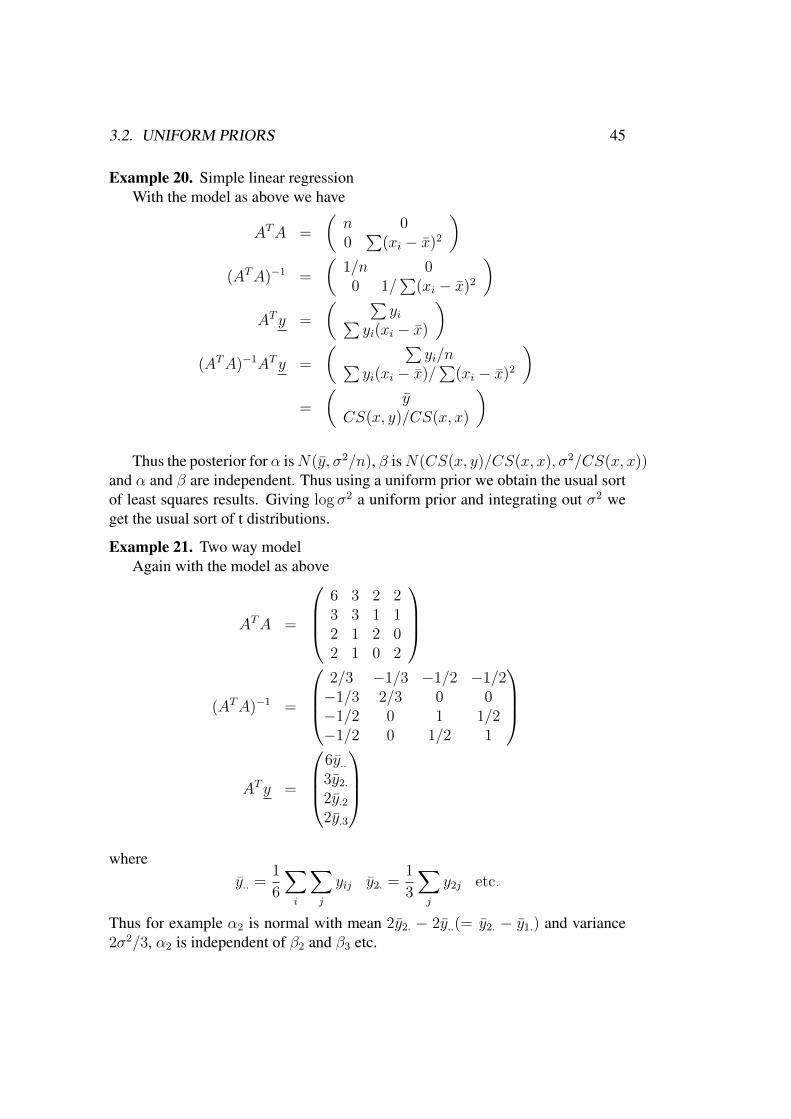
Example 20. Simple linear regressionWith the model as above we have

ATA =

(n 00∑

(xi − x)2

)(ATA)−1 =

(1/n 00 1/

∑(xi − x)2

)ATy =

( ∑yi∑

yi(xi − x)

)(ATA)−1ATy =

( ∑yi/n∑

yi(xi − x)/∑

(xi − x)2

)=

(y

CS(x, y)/CS(x, x)

)

Thus the posterior for α isN(y, σ2/n), β isN(CS(x, y)/CS(x, x), σ2/CS(x, x))and α and β are independent. Thus using a uniform prior we obtain the usual sortof least squares results. Giving log σ2 a uniform prior and integrating out σ2 weget the usual sort of t distributions.

Example 21. Two way modelAgain with the model as above

ATA =

6 3 2 23 3 1 12 1 2 02 1 0 2

(ATA)−1 =

2/3 −1/3 −1/2 −1/2−1/3 2/3 0 0−1/2 0 1 1/2−1/2 0 1/2 1

ATy =

6y..3y2.2y.22y.3

where

y.. =1

6

∑i

∑j

yij y2. =1

3

∑j

y2j etc.

Thus for example α2 is normal with mean 2y2. − 2y..(= y2. − y1.) and variance2σ2/3, α2 is independent of β2 and β3 etc.


3.3 Normal priorsWe now consider the following linear model

y ∼ N(A1θ1, C1)

where A1, C1 are known. Suppose we adopt a normal prior for θ1.

θ1 ∼ N(µ,C2)

where µ,C2 are known.This is called a two stage model and was first studied by Lindley and Smith in

1972 (J. Roy. Statist. Soc., B.). The assumption of a normal prior is linked to theidea that the components of θ1 are exchangeable, we shall return to this idea later.

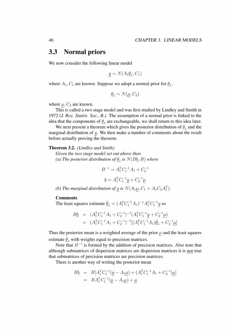
We next present a theorem which gives the posterior distribution of θ1 and themarginal distribution of y. We then make a number of comments about the resultbefore actually proving the theorem.

Theorem 3.2. (Lindley and Smith)Given the two stage model set out above then(a) The posterior distribution of θ1 is N(Bb,B) where

B−1 = AT1C−11 A1 + C−12

b = AT1C−11 y + C−12 µ

(b) The marginal distribution of y is N(A1µ,C1 + A1C2AT1 ).

CommentsThe least squares estimate θ1 = (AT1C

−11 A1)

−1AT1C−11 y so

Bb = (AT1C−11 A1 + C−12 )−1(AT1C

−11 y + C−12 µ)

= (AT1C−11 A1 + C−12 )−1[(AT1C

−11 A1)θ1 + C−12 µ]

Thus the posterior mean is a weighted average of the prior µ and the least squaresestimate θ1 with weights equal to precision matrices.

Note that B−1 is formed by the addition of precision matrices. Also note thatalthough submatrices of dispersion matrices are dispersion matrices it is not truethat submatrices of precision matrices are precision matrices.

There is another way of writing the posterior mean

Bb = B[AT1C−11 (y − A1µ) + (AT1C

−11 A1 + C−12 )µ]

= BAT1C−11 (y − A1µ) + µ

3.3. NORMAL PRIORS 47

The quantity (y − A1µ) is the deviation between the observation y and its un-conditional expectation A1µ, ie the difference between the observed value y andwhat we expected the value to be. The quantity BAT1C

−11 is called a filter. This

expression shows how we update our prior mean µ.We will often use the posterior mean of θ1 as an estimate. We will denote this

posterior mean by θ∗1

Proof. (a) If we multiply likelihood by prior we get K exp(−Q/2) where

Q = (y − A1θ1)TC−11 (y − A1θ1) + (θ1 − µ)TC−12 (θ1 − µ)

= θT1AT1C−11 A1θ1 + θT1C

−12 θ1 − 2θT1A

T1C−11 y − 2θT1C

−12 µ+ yTC−11 y

+µTC−12 µ

= θT1 (AT1C−11 A1 + C−12 )θ1 − 2θT1 (AT1C

−11 y + C−12 µ) + yTC−11 y + µTC−12 µ

= θT1B−1θ1 − 2θT1 b+ yTC−11 y + µTC−12 µ

= (θ1 −Bb)TB−1(θ1 −Bb) + yTC−11 y + µTC−12 µ− bTBb

Thus the posterior of θ1 is proportional to

exp[(−1/2)(θ1 −Bb)TB−1(θ1 −Bb)]

and hence the result follows.(b) We need a lemma to prove this result.

Lemma 3.3. If v ∼ N(0, C) then Av ∼ N(0, ACAT ).

Thus we can write

y = A1θ1 + u u ∼ N(0, C1)

θ1 = µ+ v v ∼ N(0, C2)

and these are independent. Thus

y = A1µ+ A1v + u

the result follows from the lemma above.

Example 22. (p = 1)We consider univariate observations with

y = (1, 1, . . . , 1)T θ C1 = σ2I µ = µ C2 = τ 2


AT1C−11 A1 = n/σ2 AT1C

−11 y =

∑yi/σ

2

AT1C−11 A1 + C−12 = (n/σ2) + (1/τ 2)

AT1C−11 y + C−12 µ = (

∑yi/σ

2) + (µ/τ 2)

and hence

Bb =(∑yi/σ

2) + (µ/τ 2)

(n/σ2) + (1/τ 2)

These are the same results as shown before in section 2.4.

Example 23. We now consider a case where n = p = 2.

y =

(y1y2

)A1 = I θ1 =

(θ1θ2

)C1 = σ2I

E[yi] = θi µ =

(µµ

)C2 =

(τ 2 ρτ 2

ρτ 2 τ 2

)Thus we are assuming observations with different means, but our beliefs aboutthese means is that they are similar (both have prior mean µ) and have correlationρ.

C−12 =1

τ 2(1− ρ2)

(1 −ρ−ρ 1

)B−1 = Iσ−2 + C−12

=

(1σ2 + 1

τ2(1−ρ2)−ρ

τ2(1−ρ2)−ρ

τ2(1−ρ2)1σ2 + 1

τ2(1−ρ2)

)Thus

B =(1− ρ2)τ 4σ4

(σ2 + τ 2)2 − ρ2τ 4

(1σ2 + 1

τ2(1−ρ2)ρ

τ2(1−ρ2)ρ

τ2(1−ρ2)1σ2 + 1

τ2(1−ρ2)

)Also

b = C−11 y + C−12 µ

=

((y1/σ

2) + (µ/τ 2(1 + ρ))(y2/σ

2) + (µ/τ 2(1 + ρ))

)Thus the posterior mean of θ1 is

(1− ρ2)τ 4σ4

(σ2 + τ 2)2 − ρ2τ 4

(1

σ2+

1

τ 2(1− ρ2)

)(y1σ2

+µ

τ 2(1 + ρ)

)+

ρ

τ 2(1− ρ2)

(y2σ2

+µ

τ 2(1 + ρ)

)=

(τ 4(1− ρ2) + σ2τ 2)y1 + ρσ2τ 2y2 + σ2(τ 2(1− ρ) + σ2)µ

(σ2 + τ 2)2 − ρ2τ 4

3.3. NORMAL PRIORS 49

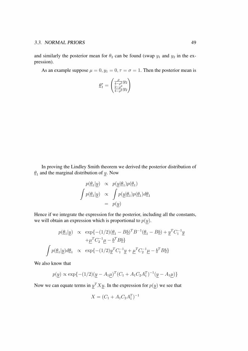
and similarly the posterior mean for θ2 can be found (swap y1 and y2 in the ex-pression).

As an example suppose µ = 0, y1 = 0, τ = σ = 1. Then the posterior mean is

θ∗1 =

(ρ

4−ρ2y22−ρ24−ρ2y2

)

In proving the Lindley Smith theorem we derived the posterior distribution ofθ1 and the marginal distribution of y. Now

p(θ1|y) ∝ p(y|θ1)p(θ1)∫p(θ1|y) ∝

∫p(y|θ1)p(θ1)dθ1

= p(y)

Hence if we integrate the expression for the posterior, including all the constants,we will obtain an expression which is proportional to p(y).

p(θ1|y) ∝ exp−(1/2)(θ1 −Bb)TB−1(θ1 −Bb) + yTC−11 y

+µTC−12 µ− bTBb∫p(θ1|y)dθ1 ∝ exp−(1/2)yTC−11 y + µTC−12 µ− bTBb

We also know that

p(y) ∝ exp−(1/2)(y − A1µ)T (C1 + A1C2AT1 )−1(y − A1µ)

Now we can equate terms in yTXy. In the expression for p(y) we see that

X = (C1 + A1C2AT1 )−1


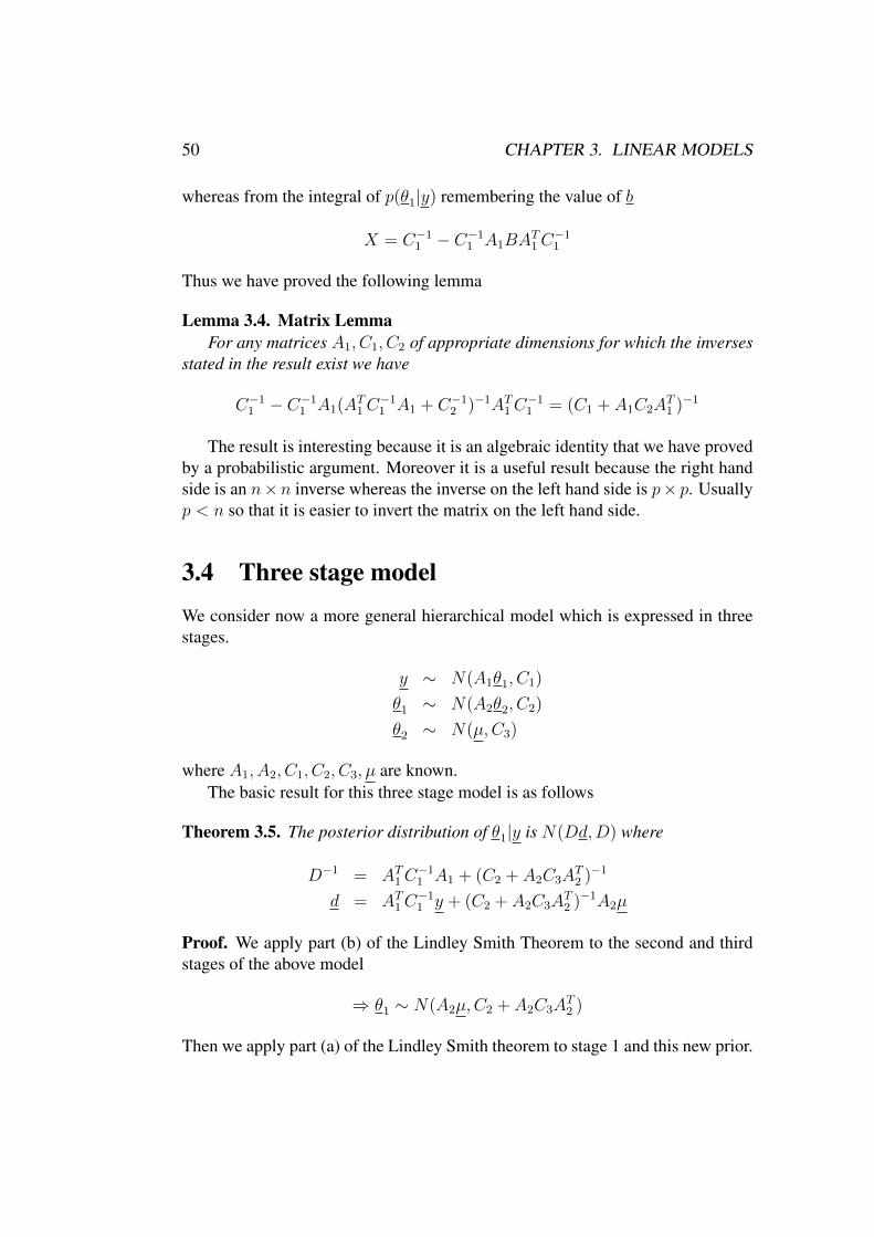
whereas from the integral of p(θ1|y) remembering the value of b

X = C−11 − C−11 A1BAT1C−11

Thus we have proved the following lemma

Lemma 3.4. Matrix LemmaFor any matrices A1, C1, C2 of appropriate dimensions for which the inverses

stated in the result exist we have

C−11 − C−11 A1(AT1C−11 A1 + C−12 )−1AT1C

−11 = (C1 + A1C2A

T1 )−1

The result is interesting because it is an algebraic identity that we have provedby a probabilistic argument. Moreover it is a useful result because the right handside is an n×n inverse whereas the inverse on the left hand side is p× p. Usuallyp < n so that it is easier to invert the matrix on the left hand side.

3.4 Three stage modelWe consider now a more general hierarchical model which is expressed in threestages.

y ∼ N(A1θ1, C1)

θ1 ∼ N(A2θ2, C2)

θ2 ∼ N(µ,C3)

where A1, A2, C1, C2, C3, µ are known.The basic result for this three stage model is as follows

Theorem 3.5. The posterior distribution of θ1|y is N(Dd,D) where

D−1 = AT1C−11 A1 + (C2 + A2C3A

T2 )−1

d = AT1C−11 y + (C2 + A2C3A

T2 )−1A2µ

Proof. We apply part (b) of the Lindley Smith Theorem to the second and thirdstages of the above model

⇒ θ1 ∼ N(A2µ,C2 + A2C3AT2 )

Then we apply part (a) of the Lindley Smith theorem to stage 1 and this new prior.

3.4. THREE STAGE MODEL 51

It is possible to extend the model to more than three stages but for most ap-plications three is enough. The three stage model reduces to a two stage model ifC3 = 0, i.e. if we know the value of θ2 exactly.

The other extreme is to take C3 → ∞ or equivalently C−13 → 0, representingvague prior knowledge about the value of θ2. The result is as follows.

Theorem 3.6. For the three stage model with C−13 → 0 the posterior distributionof θ1|y is N(D0d0, D0) where

D−10 = AT1C−11 A1 + C−12 − C−12 A2(A

T2C−12 A2)

−1AT2C−12

d0 = AT1C−11 y

Proof. The result for the precision follows from the matrix lemma by rewritingthe expression for D−1 and letting C−13 → 0.

The result for d0 follows since

(C2 + A2C3AT2 )−1A2 = C−12 − C−12 A2(A

T2C−12 A2)

−1AT2C−12 A2

= C−12 A2 − C−12 A2

= 0

Thus writing F = C−12 − C−12 A2(AT2C−12 A2)

−1AT2C−12 we see the posterior

mean is(AT1C

−11 A1 + F )AT1C

−11 y

and the posterior dispersion matrix is

(AT1C−11 A1 + F )−1

Before we consider an example we note a lemma on the inverse of a certainsort of patterned matrix.

Lemma 3.7.(aIn + bJn)−1 =

1

aIn −

b

(a+ nb)aJn

for a > 0, b 6= −(a/n) where In is an n × n identity matrix and Jn is an n × nmatrix of ones.

The lemma is easily verified by direct multiplication noting that J2n = nJn.

Example 24. We consider a one-way model where

yi ∼ N(θi, σ2) i = 1, . . . , n


where i represents a treatment or group. In practice yi will be the mean (a suffi-cient statistic) of m observations. We complete the model by assuming

θi ∼ N(µ, τ 2)

and that our knowledge about µ is vague so that C−13 → 0. Thus we have

A1 = In C1 = σ2In A2 = 1n C2 = τ 2In

where 1n is a column of ones.Substituting these values into the results we have obtained we see that

D−10 = σ−2In + In − 1n(1Tn1n)−11Tnτ−2

Now 1Tn1n = n and 1n1Tn = Jn so

D−10 = (σ−2 + τ−2)In − (1/nτ 2)Jn

and hence applying the lemma

D0 = (σ−2 + τ−2)−1In + (σ2/nτ 2)Jn

Alsod0i = yi/σ

2

Now Iny = y and Jny = (∑yi)1n = (ny)1n and so

θ∗i = E[θi|y] = (σ−2 + τ−2)−1(yi/σ2) + (y/τ 2)

We can thus write this asθ∗i = ρyi + (1− ρ)y

where ρ = τ 2/(σ2 + τ 2) and we see that 0 ≤ ρ ≤ 1. Comparing this result withthat when µ is known, in effect we replace the unknown µ by y.

We can also find the posterior variance of θi by considering a diagonal elementof D0.

V ar[θi|y] = (σ−2 + τ−2)−11 + (σ2/nτ 2)

= σ2 − (1− 1/n)σ4

σ2 + τ 2

< σ2

Similarly the posterior covariance of θi and θj is given by a non-diagonal elementof D0

Cov[θi, θj|y] =σ4/n

σ2 + τ 2> 0

3.5. EXCHANGEABILITY 53

Hence using the formula V ar[X−Y ] = V ar[X]+V ar[Y ]−2Cov[X, Y ] we seethat

V ar[θi − θj|y] =2σ2τ 2

σ2 + τ 2

Note that this is less than 2σ2 which is the classical least squares value. Thus

θi − θj|y ∼ N(ρ(yi − yj), 2σ2ρ)

There is another way of deriving θ∗ when it is not so easy to invert D−10 . Weare essentially solving the equations

D−10 θ∗ = d

Writing out the ith of these equations we see

(σ−2 + τ−2)θ∗i − (1/nτ 2)∑

θ∗i = σ−2yi

If we sum both sides of this equation for i = 1, . . . , n we obtain

σ−2∑

θ∗i = σ−2∑

yi

Hence∑θ∗i =

∑yi and we can substitute this to give the same answer as before.

3.5 ExchangeabilitySuppose yi ∼ N(θi, σ

2) for i, . . . , n, e.g. yi might be the observation on the ithvariety in a field trial with average yield θi. In considering the prior knowledgeabout θi it may be reasonable to assume the θis are exchangeable. This means thatour beliefs about the θis are symmetric. Our beliefs about θ1 is the same as ourbelief about θ6. Our joint belief about θ2 and θ3 is the same as our joint beliefabout θ1 and θ5 and so on. It follows that the θi’s will have a common distributionfunction. If we make the additional assumption that this distribution is normalwe see that θi ∼ N(µ,C2) and we end up with the two stage model we havediscussed.

We must consider the exchangeability assumption carefully. For example ifsome of the varieties are controls and others experimental the assumption is notjustifiable. But we might assume exchangeability within the controls and sepa-rately within the experimental varieties.

Example 25. We consider a randomised block design.

E[yij] = µ+ αi + βj 1 ≤ i ≤ t 1 ≤ j ≤ b


with errors independent and N(0, σ2).

A1 =

1b 0 . . . . . . 0 Ib0 1b . . . . . . 0 Ib

1bt...

... . . . ......

...... . . . ...

...0 0 . . . . . . 1b Ib

Also θT1 = (µ, α1, . . . , αt, β1, . . . , βb).

For the second stage it might be reasonable to assume that the αi are ex-changeable and similarly the βj are exchangeable. (It would not be reasonableif the treatments were increasing levels of a single fertiliser for example). We thustake

αi ∼ N(0, σ2α) βj ∼ N(0, σ2

β) µ ∼ N(ω, σ2µ)

The means are chosen to be zero for the α’s and β’s so that they can be regarded asdeviations from an average level. Thus we are making the following assignments

C1 = σ2I, C2 = diag(σ2µ, σ

2α, . . . , σ

2α, σ

2β, . . . , σ

2β), µT = (ω, 0, . . . , 0).

The Lindley Smith theorem tells us that the posterior distribution of θ1 isN(Bb,B)where

B−1 = σ−2AT1A1 + C−12

b = σ−2AT1 y + C−12 µ.

We assume that our prior knowledge about µ is vague so that σ−2µ → 0 and henceC−12 µ→ 0. It follows that θ∗1 satisfies

(AT1A1 + σ2C−12 )θ∗1 = AT1 y (3.1)

These equations differ from the usual least squares equations only by inclusion ofσ2C−12 . Now

AT1A1 =

bt b1Tt t1Tbb1t bIt Jt,bt1b Jb,t tIb

and hence

AT1A1 + σ2C−12 =

bt b1Tt t1Tbb1t (b+ σ2/σ2

α)It Jt,bt1b Jb,t (t+ σ2/σ2

β)Ib

3.6. UNKNOWN VARIANCES 55

Also(AT1 y)T = (bty.., by1., . . . , byt., ty.1, . . . , ty.b

After a little algebra it is clear that the solution to (3.1) is

µ∗ = y.. α∗i = (bσ2α + σ2)−1bσ2

α(yi. − y..) β∗j = (tσ2β + σ2)−1tσ2

β(y.j − y..)

We may compare these with the usual least squares estimates

µ = y.. αi = yi. − y.. βj = y.j − y..

3.6 Unknown variancesSo far we have assumed all variances are known. In practice, of course, this isunlikely to be true. We shall outline the approach that might be taken. In Chapter4 we shall consider another, better, solution to this problem.

For a one-way model

yij ∼ N(θi, σ2) i = 1, . . . , n j = 1, . . . ,m

with prior θi ∼ N(µ, τ 2) and a vague prior on µ, suppose σ2 and τ 2 are unknown.Lindley and Smith suggest the following independent priors for σ2 and τ 2,

λ1ν1σ2∼ χ2

ν1

λ2ν2τ 2∼ χ2

ν2.

With these priors we find

p(θ|y) ∝ [S2+n∑

(yi.−θi)2+ν1λ1]−(nm+ν1)/2[

∑(θi− θ.)2+ν2λ2]

−(m+ν2−1)/2

where S2 =∑∑

(yij− yi.)2. This is a product of two multivariate t distributions.Inference about σ2 and τ 2 is not easy – approximate methods exist to make jointestimates of θ, σ2, τ 2 based on posterior modes.

As an alternative Box and Tiao suggest using the prior

p(σ2, τ 2) ∝ 1

σ2

1

σ2 +mτ 2

which is approximately non-informative. It has the defect that it depends on mwhich means our prior is dependent on how much data we have! We also mightask what to do if the mi’s are different. In practice it provides answers which givea good approximation so long as τ 2 is not very much smaller than σ2.

Additional Reading. Chapter 8 of Lee

Chapter 4

Approximate methods

4.1 Numerical IntegrationAs we mentioned in section 2.1 integration is central to Bayesian statistics and itis sometimes necessary to calculate integrals numerically. In this section we shallgive a simple illustration of this.

We shall consider the problem of making inferences about the location param-eter θ of a Cauchy distribution with pdf

p(x|θ) = π−1[1 + (x− θ)2]−1 −∞ < x <∞

If we assume a locally uniform prior then the posterior is given by

p(θ|x) ∝n∏i=1

[1 + (xi − θ)2]−1

Suppose the data are 5 observations (11.4, 7.3, 9.8, 13.7, 10.6). We may writep(θ|x) = cH(θ) where

H(θ) = 105[1 + (11.4− θ)2]−1[1 + (7.3− θ)2]−1 . . . [1 + (10.6− θ)2]−1

the factor 105 is a convenient multiplier and c is the normalising constant. We maydraw H(θ) and this may be sufficient for our purposes. If we wish to determinethe posterior exactly then we have to determine the value of c given by

c−1 =

∫ ∞−∞

H(θ)dθ

One possibility would be to draw H(θ) carefully on squared paper and count thesquares! Another possibility is to use numerical integration.

57

58 CHAPTER 4. APPROXIMATE METHODS

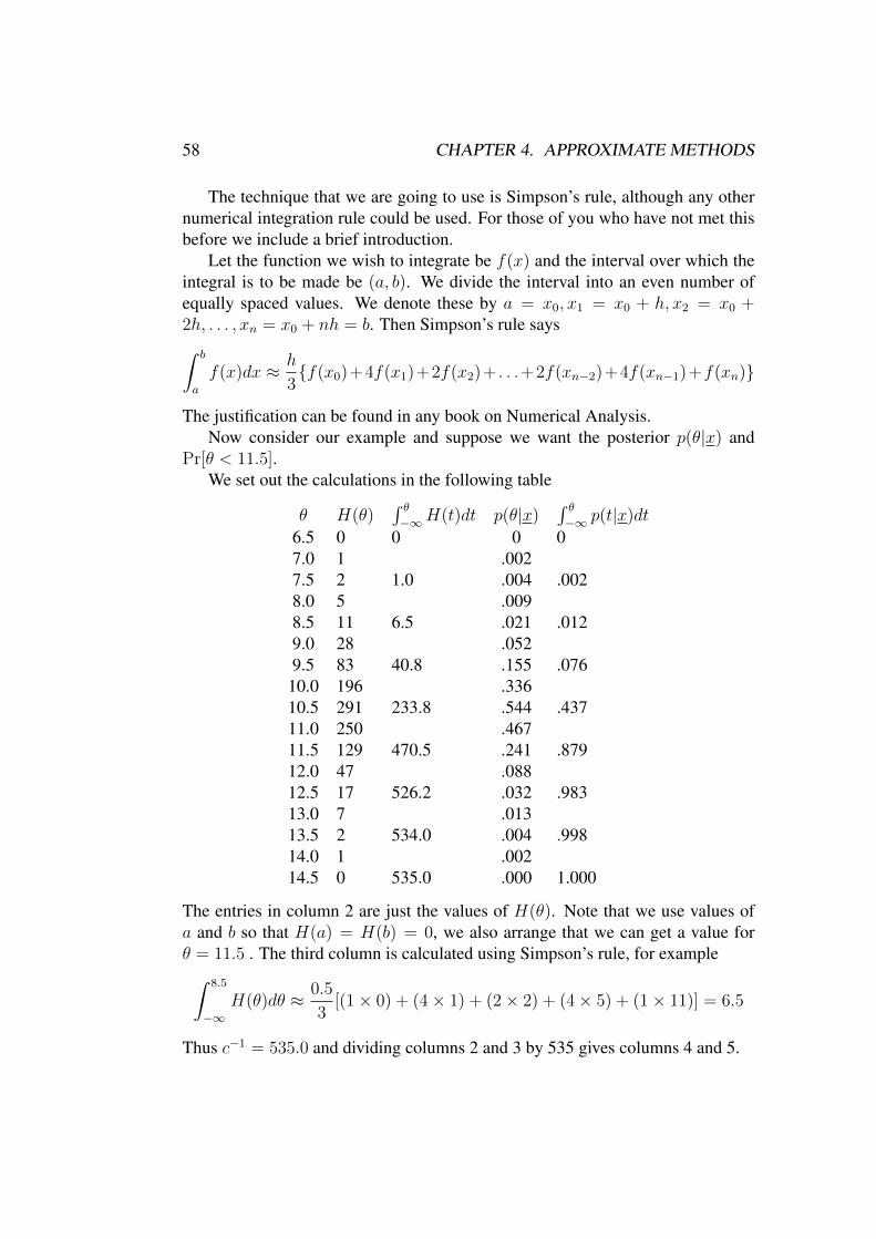
The technique that we are going to use is Simpson’s rule, although any othernumerical integration rule could be used. For those of you who have not met thisbefore we include a brief introduction.

Let the function we wish to integrate be f(x) and the interval over which theintegral is to be made be (a, b). We divide the interval into an even number ofequally spaced values. We denote these by a = x0, x1 = x0 + h, x2 = x0 +2h, . . . , xn = x0 + nh = b. Then Simpson’s rule says∫ b

a

f(x)dx ≈ h

3f(x0)+4f(x1)+2f(x2)+ . . .+2f(xn−2)+4f(xn−1)+f(xn)

The justification can be found in any book on Numerical Analysis.Now consider our example and suppose we want the posterior p(θ|x) and

Pr[θ < 11.5].We set out the calculations in the following table

θ H(θ)∫ θ−∞H(t)dt p(θ|x)

∫ θ−∞ p(t|x)dt

6.5 0 0 0 07.0 1 .0027.5 2 1.0 .004 .0028.0 5 .0098.5 11 6.5 .021 .0129.0 28 .0529.5 83 40.8 .155 .076

10.0 196 .33610.5 291 233.8 .544 .43711.0 250 .46711.5 129 470.5 .241 .87912.0 47 .08812.5 17 526.2 .032 .98313.0 7 .01313.5 2 534.0 .004 .99814.0 1 .00214.5 0 535.0 .000 1.000

The entries in column 2 are just the values of H(θ). Note that we use values ofa and b so that H(a) = H(b) = 0, we also arrange that we can get a value forθ = 11.5 . The third column is calculated using Simpson’s rule, for example∫ 8.5

−∞H(θ)dθ ≈ 0.5

3[(1× 0) + (4× 1) + (2× 2) + (4× 5) + (1× 11)] = 6.5

Thus c−1 = 535.0 and dividing columns 2 and 3 by 535 gives columns 4 and 5.

4.2. ASYMPTOTIC NORMALITY OF THE POSTERIOR DISTRIBUTION 59

Of course the answers are only approximate but will be good enough for allpractical purposes.

We could also calculate the posterior mean of θ by adding a column θH(θ)and working out its integral. Then E[θ|x] would be this integral divided by 535.

We could also put in a proper prior for θ, multiply H(θ) by the values of p(θ)before integrating.

There was a lot of research effort in the 1980’s into finding efficient ways ofintegration for more than one parameter. It was found that it is feasible to dealwith problems with 15 or 20 parameters using numerical integration. However,research in this area has been eclipsed by the discovery of efficient stochasticsimulation methods. See section 4.4.

4.2 Asymptotic normality of the posterior distribu-tion

Suppose a posterior distribution p(θ | y) is unimodal and roughly symmetric. It isoften convenient to approximate this posterior by a normal distribution centred atthe mode. To see the justification for this suppose first that θ is a one dimensionalparameter. Consider a Taylor expansion of log p(θ | y) centred at the posteriormode θ

log p(θ | y) = log p(θ | y)+(θ−θ)[d

dθlog p(θ | y)

]θ=θ

+1

2(θ−θ)2

[d2

dθ2log p(θ | y)

]θ=θ

+· · ·

Now by the definition of the posterior mode[ddθ

log p(θ | y)]θ=θ

= 0, so ignoringhigher order terms and exponentiating both sides we have

p(θ | y) ≈ constant× exp

(−1

2

[− d2

dθ2log p(θ | y)

]θ=θ

(θ − θ)2).

We define the observed information I(θ) as

I(θ) =

[− d2

dθ2log p(θ | y)

].

Thus we see that approximately the posterior distribution of θ is normal with meanθ, the posterior mode and variance I(θ)−1, the reciprocal of the observed infor-mation evaluated at the posterior mode.

Example 26. Suppose y1, . . . , yn is a random sample from a Poisson distributionwith mean θ and the prior distribution for θ is gamma with parameters α and β.


We have seen that the posterior for θ is gamma with parameters α +∑yi and

β + n. Therefore

log p(θ | y) = −(β + n)θ + (α +∑

yi − 1) log θ + constant.

Differentiating with respect to θ we have

d

dθlog p(θ | y) = −(β + n) +

(α +∑yi − 1)

θ,

so setting this equal to zero and solving we find the posterior mode, θ, is given by

θ =α +

∑yi − 1

β + n.

Now differentiating again we find

d2

dθ2log p(θ | y) = −(α +

∑yi − 1)

θ2,

so the observed information is given by

I(θ) =(α +

∑yi − 1)

θ2.

Substituting in for θ we find

I(θ) =(β + n)2

α +∑yi − 1

.

Therefore the posterior distribution of θ is approximately normal with mean α+∑yi−1

β+n

and variance α+∑yi−1

(β+n)2.

We can find a similar result when θ is a p vector of parameters. We have theTaylor expansion

log p(θ | y) = log p(θ | y) +1

2(θ − θ)T

[d2

dθ2log p(θ | y)

]θ=θ

(θ − θ) + · · ·

since[ddθ

log p(θ | y)]θ=θ

= 0. It is then clear that

θ | y ∼ N(θ, I(θ)−1)

where the i, j entry of the p× p matrix I(θ) is given by

I(θ)i,j = − d2

dθidθjlog p(θ | y).

4.2. ASYMPTOTIC NORMALITY OF THE POSTERIOR DISTRIBUTION 61

Example 27. Suppose y1, . . . , yn is a random sample from a normal distributionwith mean µ and precision ξ and the prior for θ = (µ, ξ) is given by p(µ, ξ) = ξ−1.Then, as we have seen in chapter 2, the posterior distribution is given by

p(µ, ξ | y) ∝ ξn/2−1 exp−ξ2

[n(y − µ)2 + (n− 1)s2

].

Therefore

log p(µ, ξ | y) = (n

2− 1) log ξ − ξ

2

[n(y − µ)2 + (n− 1)s2

]+ constant.

Differentiating with respect to µ

d

dµlog p(µ, ξ | y) = ξn(y − µ)

so µ = y.Differentiating with respect to ξ

d

dξlog p(µ, ξ | y) = (

n

2− 1)ξ−1 − 1

2

[n(y − µ)2 + (n− 1)s2

].

Setting this equal to zero and solving, remembering that µ = y, we find thatξ = (n−2)

(n−1)s2 . Now the second derivatives are given by

d2 log p(µ, ξ | y)

dµ2= −nξ


dµdξ= n(y − µ)


dξ2= −

(n− 2

2ξ2

)so

I(θ) =

(nξ 00 n−2

2ξ2

)and hence

I(θ)−1 =

((nξ)−1 0

0 2ξ2

n−2

).

Substituting for ξ we see that

(µ, ξ) | y .∼ N

((yn−2

(n−1)s2

),

((n−1)s2n(n−2) 0

0 2(n−2)(n−1)2s4

)).


In the univariate case we can say that if n is large then the posterior of θ is ap-proximately normal and an approximate 95% credible interval is θ± 2(I(θ))−1/2.

Note that if the prior for θ is locally uniform then p(θ | y) ∝ p(y | θ) and theposterior mode is the maximum likelihood estimate.

Example 28. Suppose y1, . . . , yn is a random sample from an exponential distri-bution with mean θ−1 and the prior for θ is p(θ) ∝ constant. Then the posteriorfor θ is given by

p(θ | y) ∝ θn exp(−θ∑

yi).

The log posterior is

log p(θ | y) = n log θ − θ∑

yi + constant.

Differentiating with respect to θ and setting equal to zero we see that the posteriormode θ = n/

∑yi which is also the maximum likelihood estimate. Differentiat-

ing again we see the information is I(θ) = θ2/n so I(θ) = (∑yi)

2/n. It followsthat an approximation to the posterior distribution of θ is given by a normal distri-bution with mean n/

∑yi and variance n/(

∑yi)

2.

With n large the effect of the prior is usually small and a normal approximationbased on the maximum likelihood estimate is always possible and likely to begood enough.

4.3 Laplace’s method for evaluating integralsIn Bayesian statistics we often want to calculate expectations which are integralsof the form

E[g(θ) | y] =

∫g(θ)p(θ | y)dθ.

For example the posterior mean of θ is

E[θ | y] =

∫θp(θ | y)dθ

=

∫θp(y | θ)p(θ)dθ∫p(y | θ)p(θ)dθ

by Bayes theorem. This is in the form of the ratio of 2 integrals. In general,assuming that g(θ) > 0 we can write the expectation of g(θ) as∫

exp−nh∗(θ)dθ∫exp−nh(θ)dθ

(4.1)

4.3. LAPLACE’S METHOD FOR EVALUATING INTEGRALS 63

where

−nh(θ) = log p(θ) + log p(y | θ),−nh∗(θ) = log g(θ) + log p(θ) + log p(y | θ).

Suppose that θ is the value that maximises −h(θ) and θ∗ is the value that max-imises −h∗(θ). Let

σ = [h′′(θ)]−12 |θ=θ

andσ∗ = [h∗′′(θ)]−

12 |θ=θ∗

then Laplace approximations to the numerator and denominator of (4.1) are givenby √

2πσ∗n−1/2 exp−nh∗(θ∗)

and √2πσn−1/2 exp−nh(θ).

It follows that (4.1) is given approximately by(σ∗

σ

)exp−n[h∗(θ∗)− h(θ)]. (4.2)

It turns out that the error is reduced when taking ratios like this, so that this isoften a very good approximation indeed.

What is the justification for these approximations? Well if we express h(θ) asa Taylor expansion about θ we see that

h(θ) ≈ h(θ) + (θ − θ)h′(θ) +1

2(θ − θ)2h′′(θ)

≈ h(θ) + 0 + (θ − θ)2 1

2σ2

since θ maximises −h and by the definition of σ. Multiplying through by −n andexponentiating both sides we have

exp[−nh(θ)] ≈ exp[−nh(θ)] exp[− n

2σ2(θ − θ)2

]and so integrating both sides gives∫

exp[−nh(θ)]dθ ≈ exp[−nh(θ)]

∫exp

[− n

2σ2(θ − θ)2

]dθ. (4.3)


The integral on the right hand side of (4.3) is the kernel of a N(θ, σ2/n) distribu-tion so its value is

√2πσ/

√n. Thus we have the Laplace approximation∫

exp[−nh(θ)]dθ ≈ exp[−nh(θ)]√

2πσ/√n.

The derivation for h∗ is similar.This technique can be extended to p dimensional parameter vectors θ by using

multivariate Taylor expansions, but this is beyond the scope of this course.

Example 29. Suppose y1, . . . , yn is a random sample from a Poisson distributionwith mean θ and that θ has a prior distribution which is gamma with parametersα and β. The true posterior is Ga(α + s, β + n) where s =

∑yi, with mean

(α + s)/(β + n) and variance (α + s)/(β + n)2. We will calculate the mean andvariance using Laplace’s approximation and see how well it does.

For the denominator of the expression for the mean we have

−nh(θ) = log p(θ) + log p(y | θ) (4.4)

= α log β + (α− 1) log θ − βθ − log Γ(α) +∑

yi log θ − nθ −∑

log yi!

Differentiating with respect to θ and setting equal to zero we see that θ = (∑yi+

α− 1)/(n+ β). Differentiating again we have

d2

dθ2h(θ) =

α− 1 +∑yi

nθ2

so

σ =

(nθ2

α− 1 +∑yi

)1/2

=

[n(∑yi + α− 1)

(n+ β)2

]1/2Now the numerator includes an extra θ,

−nh∗(θ) = log θ − nh(θ).

Comparing with (4.4)the only difference is that the coefficient of log θ is α ratherthan α− 1. It follows that θ∗ = (

∑yi + α)/(n+ β) and

σ∗ =

[n(∑yi + α)

(n+ β)2

]1/2.

Substituting these values into (4.2) the approximate value of the posterior mean is

4.4. GIBBS SAMPLING 65

given by

E[θ | y] ≈( ∑

yi + α∑yi + α− 1

)1/2

exp[(∑

yi + α) log θ∗

−(β + n)θ∗ − (∑

yi + α− 1) log θ + (β + n)θ]

≈( ∑

yi + α∑yi + α− 1

)1/2

exp[(∑

yi + α) log

(∑yi + α

n+ β

)−(∑

yi + α)− (∑

yi + α− 1) log

(∑yi + α− 1

n+ β

)+ (∑

yi + α− 1)]

Similarly we can find the variance. We calculate this as the expectation of θ2

minus the square of the mean. Note that in calculating the expectation of θ2 in thenumerator the coefficient of log θ is α+ 1. Straightforward algebra then gives theapproximation as

E[θ2 | y] ≈(∑

yi + α + 1∑yi + α− 1

)1/2

exp[(∑

yi + α + 1) log

(∑yi + α + 1

n+ β

)−(∑

yi + α + 1)− (∑

yi + α− 1) log

(∑yi + α− 1

n+ β

)+ (∑

yi + α− 1)]

To investigate the Laplace approximation suppose n = 5,∑yi = 10, α =

2, β = 1, so that the sample and prior means agree. The true posterior meanis 2.0 and the variance 1/3. The approximation to the mean is 2.00126. Theapproximation to E[θ2 | y] = 4.33838, so that the approximation to the varianceis 4.33838− 2.001262 = 0.33334. In this case the approximations are very good.

Suppose now that α = 3, the other quantities remain as they were. Now thereis some disagreement between the prior and the data. The true mean is 21

6and the

variance is 0.36111. The approximations give 2.1678 for the mean and 0.36121for the variance. Again they are very good.

4.4 Gibbs sampling

4.4.1 IntroductionA number of Monte Carlo Markov chain (MCMC) methods have recently beenintroduced into Bayesian statistics. They allow a wide range of problems to besolved. Another general name for these methods is Stochastic Simulation. Thebasic idea is to simulate from the distribution we are interested in and use thesimulated sample to make inferences. Gibbs sampling is one of these methods. Itis one of the simplest and will provide a good introduction to the ideas.


4.4.2 The basic algorithm

Suppose we have a problem involving a number of parameters. We have the likeli-hood and the priors we want to calculate the joint and marginal posterior distribu-tions of the parameters, posterior means, variances and covariances and predictivedistributions. We don’t know how to do the necessary integration analytically (itmay not be possible) and numerical methods are not recommended for the num-ber of parameters we have. If we can find the conditional (posterior) distributionof each parameter and we can simulate from this distribution then we can use theGibbs sampler to find a sample from the joint posterior distribution. Technicallywhat we are doing is building a Markov chain whose limiting distribution is therequired posterior. It doesn’t matter if you don’t know about Markov chains allyou need to know is the technique.

To fix ideas, suppose we have a problem with three parameters θ, δ and φ.The likelihood is p(x|θ, δ, φ) and the prior p(θ, δ, φ). Suppose we can find theconditional distributions

p(θ|δ, φ, x), p(δ|φ, θ, x), p(φ|θ, δ, x)

and we can simulate from them. The Gibbs sampler is an iterative scheme thatproceeds as follows:

Step 1 Choose initial estimates θ0, δ0, φ0

Step 2 Given current estimates θi, δi, φi

simulate new valuesθi+1 from p(θ|δi, φi, x)δi+1 from p(δ|φi, θi+1, x)φi+1 from p(φ|θi+1, δi+1, x)

Step 3 Return to step 2The sequence (θ, δ, φ)i i = 1, 2, . . . is a realisation of a Markov chain which,

under mild regularity conditions, has equilibrium distribution p(θ, δ, φ|x), the jointposterior distribution of θ, δ, φ.

Often we run the chain for a burn-in period of length L, say, so that the initialvalues are ‘forgotten’. Then we might take all the values thereafter (or maybeevery fifth or tenth value to reduce serial correlation) as our sample from the pos-terior. Ergodic theory, which is beyond the scope of this course, tells us that theposterior mean of θ, say, can be estimated by

1

t

L+t∑i=L+1

θi

for suitably large t.


If we want to see a picture of the posterior density of θ we can use a tech-nique known as Kernel density estimation. This is also beyond the scope of thiscourse but the idea is similar to drawing histograms. You can think of drawinga histogram as drawing lots of little uniform densities about the observed points.For Kernel density estimation we use other densities (often the normal) so that theresulting picture is smooth.

The predictive density of a new observation y can be estimated as

p(y|x) =1

t

L+t∑i=L+1

P (y|θi, δi, φi)

since p(y|x) = E[p(y|θ, δ, φ) | x].

Example 30. As a first example we consider a Poisson hierarchical model. Atthe first stage we have observations sj which are Poisson with mean tjλj forj = 1, 2, . . . , p where tj is known. We assume that the λj are independentand identically distributed with Ga(α, β) prior distributions. The parameter αis known but β is unknown and is given a Ga(γ, δ) distribution where γ and δare known. We thus have p + 1 unknown parameters, the λ’s and β. The jointposterior of the unknown parameters is, by Bayes theorem,

p∏j=1

(λjtj)sj exp(−λjtj)sj!

×p∏j=1

Γ(α)−1βαλα−1j exp(−βλj)×Γ(γ)−1δγβγ−1 exp(−δβ).

To find the conditional distributions of the λ’s and β we have to pick out therelevant terms from this posterior.

Consider first the conditional distribution of λk given β, the data (the sj’s) andthe other λ’s. We see that

p(λk|β, λj(j 6= k), data) ∝ λskk exp(−λktk)λα−1k exp(−λkβ)

so the required conditional distribution is Ga(α + sk, β + tk).Now consider the conditional distribution of β given the data and the λ’s. We

see thatp(β|λ, data) ∝ βpα exp(−

∑λjβ)βγ−1 exp(−δβ)

so the required conditional distribution is Ga(pα + γ,∑λj + δ).

Thus given suitable starting values for the unknown parameters the Gibbs sam-pler proceeds by drawing

λi+1j ∼ Ga(α + sj, β

i + tj) j = 1, . . . , p

βi+1 ∼ Ga(pα + γ,∑

λi+1j + δ)


Example 31. As a second example we will consider a hierarchical linear modelwith unknown variances. We consider a one-way model with different variances(precisions) for each treatment group. Thus we have

Yij ∼ No(θi, hi) i = 1, . . . , I j = 1, . . . , ni.

We assume the means θi have a normal prior

θi ∼ No(µ, ξ)

and the precisions hi have a gamma prior

hi ∼ Ga(a12,b12

).

At the third stage we assume a normal prior for µ,

µ ∼ No(µ0, ξ0)

with µ0 and ξ0 known and a gamma prior for ξ

ξ ∼ Ga(a22,b22

).

Note that Yi ∼ No(θi, nihi).The full conditionals can be obtained using the usual sort of calculations as

we had in Chapter 2.For the distribution of θi we are simply using the result for a normal mean with

known variance. Thus

θi | y, hi, µ, ξ ∼ No

(nihiYi + ξµ

nihi + ξ, nihi + ξ

)i = 1, . . . , I.

Similarly the distribution of hi is obtained using the result for a precision withknown mean

hi | y, θi ∼ Ga

(a1 + ni

2,b1 +

∑j(Yij − θi)2

2

)i = 1, . . . , I.

To obtain the distribution of µ note that∑i θiI∼ No(µ, Iξ) (4.5)

and putting this together with the prior for µ we have

µ | y, θ, ξ ∼ No

(ξ∑θi + ξ0µ0

Iξ + ξ0, Iξ + ξ0

).


Finally putting together (4.5) and the prior for ξ we see that

ξ | y, θ, µ ∼ Ga

(a2 + I

2,b2 +

∑(θi − µ)2

2

).

Since all the full conditionals are normal and gamma distributions, the simulationis straightforward.

4.4.3 Constraints on parameters

We saw in section 2.5 how to allow for constraints on parameters. In practicewe may need to do integrations over awkward areas. Gibbs sampling enables thecalculations to be done in a straightforward way.

Consider the Gibbs sampling algorithm presented above, but suppose we havethe constraints 0 ≤ θ ≤ δ ≤ φ ≤ ∞. We can use a rejection technique as follows.Step 1 Choose initial estimates θ0 ≤ δ0 ≤ φ0

Step 2 Given current estimates θi, δi, φi

simulate new valuesθi+1 from p(θ|δi, φi, x)If 0 ≤ θi+1 ≤ δi accept, otherwise simulate againδi+1 from p(δ|φi, θi+1, x)If θi+1 ≤ δi+1 ≤ φi accept, otherwise simulate againφi+1 from p(φ|θi+1, δi+1, x)If δi+1 ≤ φi+1 accept, otherwise simulate again.

Step 3 Return to step 2Alternatively, for some distributions it is possible to draw directly from the

constrained distribution.

4.4.4 Missing data problems

In general there is no problem with missing data. We treat the missing data as extraparameters. Given the values of the missing data we can generate the parameters.Given the values of the parameters we can simulate the missing values. We willillustrate again using our Gibbs sampling algorithm. Suppose one data value, xnsay, is missing. Denote the remaining data as x(n).


Step 1 Choose initial estimates θ0, δ0, φ0, x0nStep 2 Given current estimates θi, δi, φi, xin

simulate new valuesθi+1 from p(θ|δi, φi, xin, x(n))δi+1 from p(δ|φi, θi+1, xin, x(n))

φi+1 from p(φ|θi+1, δi+1, xin, x(n))

xi+1n from p(x|θi+1, δi+1, φi+1)

Step 3 Return to step 2.

Example 32. We consider a simple linear regression model with censoring. Ourmodel is that

Yij ∼ No(α + βxi, ξ) i = 1, . . . , k j = 1, . . . , ni.

But there is a censoring value di such that at each setting of xi we cannot observethe value of Yij . Thus we observe Zij where

Zij =

Yij Yij ≤ di,

di Yij > di.

We include the unobserved Yij as parameters in the model. Assuming normalpriors for α and β and a gamma prior for ξ it is straightforward to find the fullconditionals based on all the data. The conditional for an unobserved Yij isNo(αc + βcxi, ξ

c) restricted to the range Yij > di where the superscript c refers tothe current value of the parameter.

4.4.5 DiscussionThere is no doubt that the introduction of Markov chain Monte Carlo methodshave revolutionised Bayesian statistics. Problems which were very difficult beforecan now be done fairly routinely. There are also other problems, mainly involvingmany parameters, which had no statistical solution, Bayesian or classical, whichnow can be tackled.

Additional Reading. Section 1.4.2 Box and Tiao, Bayesian Inference in Statisti-cal Analysis, Section 9.4 of Lee.

Chapter 5

Criticisms and Answers

Although there are many (and a steadily increasing number of) statisticians us-ing Bayesian methods there are still a number of criticisms made against thesemethods.

The principal criticisms are the difficulty of choosing the prior distributionand a perceived lack of objectivity. There are a number of answers to these crit-icisms. Firstly any paradigm involving uncertainty will involve some subjectiveelements, Bayesians make this subjectivity explicit and have to justify their sub-jective choices. Often the likelihood (or model) is more important for the finalinference than the prior and choice of model is at least partially subjective. Asensitivity analysis should always be carried out to identify the crucial aspects ofthe model and the prior.

Some are only willing to accept a frequency definition of probability but thisessentially means accepting a (subjective) assumption of exchangeability. Theaxioms underlying subjective probability are as convincing as any others.

It is important in reporting results that Bayesian analysts give both the likeli-hood and prior used so that others can compare the answers with those obtainedusing their prior distributions.

We would acknowledge that the mathematics involved, mainly integration, canbe more difficult than using likelihood methods, mainly differentiation, but this isnot a valid reason not to use Bayesian methods.

The main advantage of the Bayesian paradigm is that it provides a coherentwhole for all problems. It provides a standard method to deal with nuisance pa-rameters, constraints on parameters and prediction, for example, rather than adhoc solutions for each particular problem.

The main disadvantages are that not many statisticians are trained in Bayesianmethods, although this is slowly changing. There is also a lack of easily availablesoftware although there have been many exciting recent developments in methodsusing stochastic simulation as we have seen in Chapter 4. It will never be totally

71

72 CHAPTER 5. CRITICISMS AND ANSWERS

straightforward to use a Bayesian approach because we do need to specify a sen-sible prior but for many problems with large numbers of parameters it is the onlyfeasible solution.

Additional Reading. G Iversen Bayesian Statistical Inference, Chapters 6, 7 and8.

mth709u/mthm042 bayesian statistics

Documents