an introduction quantum computing - · pdf fileacknowledgments special thanks are given to...

An Introduction to Quantum Computing

Michal Charemza

University of Warwick

March 2005

Acknowledgments

Special thanks are given to Steve Flammia and Bryan Eastin, authors of theLATEX package, Qcircuit, used to draw all the quantum circuits in this document.This package is available online at http://info.phys.unm.edu/Qcircuit/.

Also thanks are given to Mika Hirvensalo, author of [11], who took the timeto respond to some questions.

1

Contents

1 Introduction 4

2 Quantum States 6

2.1 Compound States . . . . . . . . . . . . . . . . . . . . . . . . . . . 82.2 Observation . . . . . . . . . . . . . . . . . . . . . . . . . . . . . . 92.3 Entanglement . . . . . . . . . . . . . . . . . . . . . . . . . . . . . 112.4 Representing Groups . . . . . . . . . . . . . . . . . . . . . . . . . 11

3 Operations on Quantum States 13

3.1 Time Evolution . . . . . . . . . . . . . . . . . . . . . . . . . . . . 133.2 Unary Quantum Gates . . . . . . . . . . . . . . . . . . . . . . . . 143.3 Binary Quantum Gates . . . . . . . . . . . . . . . . . . . . . . . 153.4 Quantum Circuits . . . . . . . . . . . . . . . . . . . . . . . . . . 17

4 Boolean Circuits 19

4.1 Boolean Circuits . . . . . . . . . . . . . . . . . . . . . . . . . . . 19

5 Superdense Coding 24

6 Quantum Teleportation 26

7 Quantum Fourier Transform 29

7.1 Discrete Fourier Transform . . . . . . . . . . . . . . . . . . . . . 297.1.1 Characters of Finite Abelian Groups . . . . . . . . . . . . 297.1.2 Discrete Fourier Transform . . . . . . . . . . . . . . . . . 30

7.2 Quantum Fourier Transform . . . . . . . . . . . . . . . . . . . . . 327.2.1 Quantum Fourier Transform in Fm

2 . . . . . . . . . . . . . 337.2.2 Quantum Fourier Transform in Zn . . . . . . . . . . . . . 35

8 Random Numbers 38

9 Factoring 39

9.1 One Way Functions . . . . . . . . . . . . . . . . . . . . . . . . . . 399.2 Factors from Order . . . . . . . . . . . . . . . . . . . . . . . . . . 409.3 Shor’s Algorithm . . . . . . . . . . . . . . . . . . . . . . . . . . . 42

2

CONTENTS 3

10 Searching 46

10.1 Blackbox Functions . . . . . . . . . . . . . . . . . . . . . . . . . . 4610.2 How Not To Search . . . . . . . . . . . . . . . . . . . . . . . . . . 4710.3 Single Query Without (Grover’s) Amplification . . . . . . . . . . 4810.4 Amplitude Amplification . . . . . . . . . . . . . . . . . . . . . . . 50

10.4.1 Single Query, Single Solution . . . . . . . . . . . . . . . . 5210.4.2 Known Number of Solutions . . . . . . . . . . . . . . . . . 5310.4.3 Unknown Number of Solutions . . . . . . . . . . . . . . . 55

11 Conclusion 57

Bibliography 59

Chapter 1

Introduction

The classical computer was originally a largely theoretical concept usually at-tributed to Alan Turing, called the Turing Machine. The first computers torealise this theory used valves as the core component for processing. This even-tually progressed to transistors, which are the building block of current proces-sors. In 1965 GordoSn Moore made an empirical observation and predictionthat the density of transistors on a chip doubles roughly every 18 months. As

1970 1975 1980 1985 1990 1995 2000 2005

104

105

106

107

108

Transistors per

integrated circuit

Figure 1.1: Moore’s Law. Source: Intel.

can be seen in Figure 1.1, this law has roughly held for about 40 years. However,this trend cannot continue indefinitely. There are differing estimates as to whenthe trend will reach its limit, one even within 6 years [13], but it is generallyagreed that a limit will be reached.

As the transistor size becomes close to the atomic scale, quantum effects,i.e. the physical laws of the very small, will begin to dominate how the tran-sistors act. However, if some, at the moment rather major, technical hurdlescan be overcome, a computer that exploits these effects, a quantum computer,could be built that have some powerful properties. It is our aim to give a briefintroduction to some of these properties.

In order to do this we will describe quantum states, and how they are repre-sented mathematically in Chapter 2. In Chapter 3 possible operations on thesestates are discussed. Chapter 4 describes how a quantum computer could do

4

CHAPTER 1. INTRODUCTION 5

anything a classical computer could do. The remaining chapters focus on al-gorithms that a classical computer cannot do, or at the very least, cannot doefficiently.

Chapter 2

Quantum States

In this chapter we introduce the concepts of how information is stored in aquantum computer, how to describe this formally, and make comparisons to theclassical case. We will also briefly, and rather informally, describe the quantumphysics that make our descriptions reasonable. Recall a Hilbert space is a com-plete inner product space over the complex numbers. For vectors in a Hilbertspace will use the Dirac notation |ψ〉.

Definition 2.0.1 (Qubit). A quantum bit, or qubit for short, is a 2-dimensionalHilbert space H2. We label an orthonormal basis of H2 by {|0〉 , |1〉}. Thestate of the qubit is an associated unit length vector in H2. If a state is equalto a basis vector then we say it is a pure state. If a state is any other linearcombination of the basis vectors we say it is a mixed state, or that the state isa superposition of |0〉 and |1〉.1

If the associated state of some qubit, that we label A say, is state |φ〉 at somemoment in time, then we often say that A has state |φ〉, or A is in state |φ〉.Example. An example of a mixed state of a qubit is

|ψ〉 = 1√2(|0〉+ |1〉).

Clearly this is a unit length vector in H2.

Two states are seen as equivalent up to a scale factor of some complexnumber α such that |α| = 1. This leads to the fact a qubit can be seen as asphere in 3D space, and the state of the qubit as a point on the sphere. In thiscase the sphere is known as the Bloch sphere [16].

A classical bit is traditionally defined as F2, and the state of the classical bitas a member of F2, i.e. either 0 or 1. Thus there are only two possible states aclassical bit can be in. However, a qubit can be in any state a |0〉+ b |1〉 wherea, b ∈ C and |a|2 + |b|2 = 1.

There are only two possible pure states for a qubit, |0〉 and |1〉. Thus thereis a similarity between a qubit in a pure state and a classical bit. A furthersimilarity is related to observation, which will be mentioned later. We can, andwill, often think about classical bits as qubits in pure states.

1There is a more general definition of quantum states as operators on Hilbert spaces. Forour purposes this definition is unnecessary.

6

CHAPTER 2. QUANTUM STATES 7

Remark. Note that what we are actually doing is trying to model a physicalsystem. For the classical case we say that the state of a bit is 0 or 1. This isjust trying to represent some physical state that can be in one of two possiblestates. If we are modelling a compact disc, 0 would represent a ‘hole’ (albeitvery small) and 1 would represent ’no hole’. If we are modelling a CPU, 1 wouldrepresent current going round part of a circuit, and 0 would represent no currentgoing round that part of a circuit. We could even just be modelling the stateof a light, either on or off. We do not want to try to model every tiny physicalpart of each of these systems. If we are just interested in seeing what can bedone with some physical system that has the property that can be in one of twostates, we just model that very property. Thus whatever we discover could, intheory, be applied to any physical system that has that property.

We are doing a similar thing here. We are making the assumption that somephysical system has a property that can be in a superposition of states (alongwith some other assumtions relating to observation and operations, which willbe discussed later), and seeing if that could lead to anything useful.

Remark 2.0.1. The Nuclear Magnetic Resonance, or NMR, quantum comput-ers, such as the one that successfully factored 15 in 2001 [23], use millions ofidentical molecules as the quantum computer. Roughly speaking the computerhad the same number of qubits as atoms in the molecule, its just that therewere millions of copies of the molecule. The spin of each of the atoms in themolecule represented the state of a qubit. We present a simplification of spin,but one could say that the spin in state up could represent |0〉, and down couldrepresent |1〉. We could label an orthonormal basis of H2 by |↑〉 and |↓〉 to makethis clearer. Due to the laws of quantum mechanics, the spin of the atom can bein a superposition of up and down at the same time, i.e. a linear combinationof |↑〉 and |↓〉.Remark 2.0.2. There is an important technical problem that must be solvedif quantum computers are ever to be practical. A superposition of states |0〉and |1〉 is known as a coherent state. A coherent state is extremely ‘unstable’.That is to say that it tends to interact with its environment, and collapse into apure state. This process is known as decoherence, and is seen to be inevitable.Algorithms that exploit quantum effects such as superposition, that we willdescribe later, are known as quantum algorithms. To apply these quantumalgorithms in the real world, decoherence time must be longer than the time torun the algorithm. Thus ways of making decoherence time longer are trying tobe found.

Remark 2.0.3. When describing quantum algorithms we will make the assump-tion that we can always initialize the state of qubits, usually to state |0〉. Itwould be very difficult to construct any sort of algorithm where the initial statewas not controllable.

Obviously we would like to think about systems larger than those of just onequbit. We now generalise the notion of a qubit as a two-dimensional Hilbertspace H2, to an n-dimensional Hilbert space Hn.

Definition 2.0.2 (Quantum System). A quantum system is an n-dimensionalHilbert Space Hn. We label an orthonormal basis on Hn by {|x1〉 , |x2〉 . . . , |xn〉}such that xi ∈ X for some finite X. The associated state of the system is a unitlength vector in Hn.


Just as for the qubit, if the associated state of some quantum system, thatwe label S say, is state |φ〉 at some moment in time, then we often say that Shas state |φ〉, or S is in state, |φ〉. We see that a general form for the state of aquantum system is

n∑

i=1

αi |xi〉 where αi ∈ C andn∑

i=1

|αi|2 = 1.

For clarity for pure states we will usually use English letters, such as |x〉, and forstates that may be mixed we will usually use Greek letters, such as |ψ〉. We willalso only ever use quantum systems that are some compound of some collectionof qubits. What is meant by compound is explained in the next section.

2.1 Compound States

Often we are interested in describing two quantum systems Hn and Hm at thesame time. For example we may, and in fact will, wish to describe the state oftwo qubits. Let us label an orthonormal basis of Hn by {|x1〉 , |x2〉 . . . , |xn〉} andlabel an orthonormal basis of Hm by {|y1〉 , |y2〉 . . . , |ym〉}. For basis states |xi〉and |yj〉 we write |xi〉 |yj〉 or just |xiyj〉 for the cartesian product (|xi〉 , |yj〉).

Definition 2.1.1 (Tensor Product of Spaces). Let Hn and Hm be quantumsystems with orthonormal bases labelled as above. The tensor product Hn⊗Hm

is defined to be the Hilbert space with basis {|xi〉 |yj〉 : i = 1 . . . n, j = 1 . . .m}.

We call Hn⊗Hm the compound system of Hn and Hm. Clearly Hn⊗Hm∼=

Hnm, and we will usually write Hn ⊗ Hm = Hnm. Thus a quantum state inHnm must be of the form

n∑

i=1

m∑

j=1

αij |xi〉 |yj〉 where αij ∈ C andn∑

i=1

m∑

j=1

|αij |2 = 1.

Example 2.1.1. Recall that we label an orthonormal basis of H2 by {|0〉 , |1〉}.Thus an example of a quantum state in H2 ⊗H2 (two qubits) is

1

2(|00〉+ |01〉+ |10〉+ |11〉).

Example 2.1.2. Another example of a quantum state in H2 ⊗H2 is

1√2(|00〉+ |11〉).

Two qubits in this state are called an EPR pair. This is a state that has causedcontroversy, and will be mentioned again later.

Consider quantum systems A and B, with A in state |ψ〉 and B in state|φ〉. We would like some way of describing the state in the compound systemA ⊗ B. Fortunately there is an easy way in which to achieve this, using thetensor product ⊗.


Definition 2.1.2 (Tensor Product of Vectors).

( n∑

i=1

αi |xi〉)⊗( m∑

j=1

βj |yj〉)

=n∑

i=1

m∑

j=1

αiβj |xiyj〉 .

Using this we can say that A ⊗ B is in state |ψ〉 ⊗ |φ〉. Tensor productsends unit length vectors to unit length vectors, so it does send quantum statesto quantum states. Since the basis representations for any states |φ〉 and |ψ〉are unique, it should be clear that A ⊗ B is in state |ψ〉 ⊗ |φ〉 if and only if Ais in state |ψ〉 and B is in state |φ〉. We call the state |ψ〉 ⊗ |φ〉 in A ⊗ B thecompound state of |ψ〉 and |φ〉. Another important notational point is that oftenthe symbol ⊗ is omitted. Because for basis states the tensor product |x〉 ⊗ |y〉is equal to the cartesian product, there is no conflict of notation when we write|x〉 |y〉.

We can easily apply the definitions of tensor products of spaces recursivelyto describe the compound of more than just two quantum systems, which wenow do for the specific case where each system is a qubit.

Definition 2.1.3 (Quantum Register). We will call H2m = H2 ⊗H2 . . . ⊗H2

(m times) a quantum register of length m. Put another way, it is the compoundsystem of m qubits.

We see a quantum register of length m has dimension 2m. Recall that{|0〉 , |1〉} is a basis of H2. Thus noting the earlier definition of tensor product,a basis of a quantum register of length m is

{|x0〉 |x1〉 . . . |xm−1〉 : xi ∈ {0, 1}}. (2.1)

Example 2.1.3. A quantum register H2 ⊗ H2 has basis {|00〉 , |01〉 , |10〉 , |11〉}.Given two states each in H2

|φ〉 =1√2(|0〉+ |1〉) ∈ H2 |ψ〉 = 1√

2(|0〉+ |1〉) ∈ H2,

we can see that their tensor product in H4 = H2 ⊗H2 is

|φ〉 ⊗ |ψ〉 = 1

2(|00〉+ |01〉+ |10〉+ |11〉). (2.2)

Remark 2.1.1. The spin of two atoms could be considered as a quantum registerof length two. As discussed in Remark 2.0.1 , the state of each can be a linearcombination of the states |↑〉 and |↓〉. Therefore the state of the compound sys-tem can be linear combination of the states |↑↑〉, |↑↓〉, |↓↑〉 and |↓↓〉 (rememberit must be a unit length linear combination).

2.2 Observation

We will now discuss what happens when we observe a quantum system. We willuse the words measure and observe interchangeably to mean the same thing.We say that an observation of the state in Hn,

n∑

j=1

αj |xj〉 ,


results in xk for some k with probability P (xk) = |αk|2. This is essentially whythe vector must be unit length: the probabilities |αi|2 must sum to 1.

The act of observation itself causes the state to collapse to the pure state|xk〉. This is a very important point! Another very important point is that theresult of measurement is probabilistic. We do not know what the result will be,only the probabilities of possible results.

If a quantum system in some pure state |x〉 is observed, there is only onepossible result, x, and the act of observation does not cause the state to change.This is another reason why we can view classical bits as quantum bits in purestates. We can observe classical bits repeatedly and they will not change - justas with quantum bits in pure states.

Remark 2.2.1. Consider the NMR quantum computer as discussed in Remarks2.0.1 and 2.1.1. Let us assume that the spin of an atom is in some super-positioned state, i.e. a superposition of both up and down. Describing thisstate formally we say that the state is a |↑〉 + b |↓〉 for some a, b ∈ C such that|a|2 + |b|2 = 1.

An observation of the system, using the NMR scanner, which is similar tothe MRI scanners used in hospitals, would result in our knowledge that the spinof the atom is either up or down. That is, would result in ↑ with probability|a|2, or with ↓ with probability |b|2.

The post-observation spin of the atom would then correspond exactly to theresult of the observation. Thus the post-observation state would be |↑〉 if theobservation resulted in ↑, or |↓〉 if the observation resulted in ↓.

We can also see that given and k0, k1, . . . , ks−1 ∈ 0 . . . n−1 distinct, and usingrudimentary probability, the probability of observing any of xk1

, xk2, . . . , xks

∈0 . . . n− 1 is equal to

s∑

l=1

P (xkl) =

s∑

l=1

|αkl|2.

We will now consider a partial measurement of a compound system. That isto say, observing one system out of a compound system. Let us have a compoundstate in Hn ⊗Hm

n∑

j=1

m∑

i=1

αij |xj〉 |yi〉 .

If we observe the first system, i.e. the one on the left, we will observe some xk.We will observe this with probability

P (xk) =m∑

i=1

P (xkyi) =m∑

i=1

|αik|2.

The state will then change to the state that corresponds to our observation.Specifically it will be projected onto the subspace spanned by |xk〉 and nor-malised to the unit norm. Thus our post-observation state is

1√P (xk)

m∑

i=1

αik |xk〉 |yi〉 .

This change of state due to observation is known as the projection postulate. Noreason for this change has been found.


2.3 Entanglement

Definition 2.3.1. Let Hn ⊗Hm = Hnm. A state |ψ〉 ∈ Hnm is decomposable(into Hn and Hm) if there are |µ〉 ∈ Hn, |ν〉 ∈ Hm such that |ψ〉 = |µ〉 ⊗ |ν〉. Astate |ψ〉 ∈ Hnm is entangled if such a decomposition does not exist.

Example 2.3.1. From Example 2.1.3 we see that by construction the state (2.2)is decomposable.

Example 2.3.2. Consider the pair 1√2(|00〉 + |11〉. This state is entangled. To

prove this we argue by contradiction, and assume it is decomposable. Thus forsome a0, a1, b0, b1 ∈ C

1√2(|00〉+ |11〉 = (a0 |0〉+ a1 |1〉)(b0 |0〉+ b1 |1〉)

= a0b0 |00〉+ a0b1 |01〉+ a1b0 |10〉+ a1b1 |11〉 .Note that we omit the tensor product symbol ⊗. Comparing coefficients on theleft and rights sides we arrive at a contradiction.

This state shows that entanglement can lead to rather bizarre results. Ob-servation of one qubit results in 0 or 1 with equal probability. However, oncethis observation is made, the post-observation state of the compound system is|00〉 if we observed 0, or |11〉 if we observed 1. If we now measure the otherqubit we thus find it is in exactly the same state as the first qubit was foundin. The act of observation on one qubit has determined the state of the otherqubit.

Remark 2.3.1. Two qubits in state as in Example 2.3.2 is known as an EPR pair,after the scientists Einstein, Podolsky and Rosen. These qubits appear to sharea link - measuring one determines the other. This appears to be independentof how far apart the qubits are physically. In 1935 EPR postulated [8] thatthis link between the particles must be due to some property of that both ofthe particles have, but is unknown, i.e. some hidden variable. However in 1964J. S. Bell [2] showed that if there is such a hidden variable, then experimentalresults should adhere to a particular inequality. However, repeatedly resultshave been found that violate this inequality, thus strongly suggesting that EPRwere wrong.

Remark 2.3.2. Entanglement has been observed in particles when have beenseparated by distances of over 50km [15] when sent through optical cable, and7.8km when transmitted through the atmosphere over Vienna, Austria [19]!

2.4 Representing Groups

One of the main reasons of using a computer is to work out results that actuallyrepresent something. Very often we wish states to represent members of Zn. Ifn = 2m for some m there is a very simple representation for each number. Wecan see that for x ∈ Z2m

x = 2m−1xm−1 + 2m−2xm−2 + . . .+ 2x1 + x0. (2.3)

where each xi ∈ {0, 1}. The xi form the binary representation of the number.So we then say that the basis vector in H2m that represents x is

|xm−1〉 |xm−2〉 . . . |x1〉 |x0〉 ,


and we often just write |x〉 for this basis vector. Using this notation, we seethat the set of all basis vectors (2.1) is equal to {|x〉 : x ∈ Z2m}.

Remember that H2m is actually the compound system of m qubits, and soobservation of this system means we are actually observing m individual qubits.Each qubit will be observed in state |0〉 or |1〉, so by equation (2.3) we candeduce which member of Z2m the compound system of the qubits, i.e. theregister, represents.

We sometimes do not care about what integer the register may represent iftaken to be a binary representation of a number. For a register of length mwe can say that a basis vector represents a member of F2

m. For example letx = (0, 1, 1, 1, 0) ∈ F2

5 The basis vector in H25 that represents this is |01110〉.We normally write |x〉 for this vector. Using this notation we see that the setof all basis vectors (2.1) is equal to {|x〉 : x ∈ F2

m}.

Chapter 3

Operations on QuantumStates

In this chapter we describe how the state of a quantum system changes in time.It may go without saying, but in order for a quantum computer to producemeaningful results, it needs to operate on quantum states and somehow changethem.

We will also show how this time evolution can be represented using matrices,we will give some examples of time evolution, and show how multiple operationson a quantum system can be represented by diagrams.

3.1 Time Evolution

We will make the assumption that there is some function that depends on timethat describes the time evolution of the system. This assumption is called thecausality principle. More formally this means that for all t ≥ 0 there are func-tions Ut : Hn → Hn such that if the state of the system at time t is |ψ(t)〉, then|ψ(t)〉 = Ut |ψ(0)〉. We will also assume that any such time evolution must benorm preserving, i.e. ‖Ut(|ψ(t)〉)‖ = ‖|ψ(t)〉‖, so each Ut sends quantum statesto quantum states. We will also make the hopefully reasonable assumption thatfor all t1, t2 ≥ 0 we have Ut1+t2 = Ut2Ut1 . We will also make the very importantassumption that each Ut is linear. To justify this assumption we would haveto go more into physics than is necessary for our purposes. We ask the readerto just accept it. We say a set of maps Ut that satisfies these assumptions iscalled a quantum time evolution. Quantum time evolution satisfies an importantproperty.

Definition 3.1.1 (Unitary). A map U : Hn → Hn is unitary if for all |ψ〉 , |φ〉 ∈Hn we have 〈ψ|Uφ〉 = 〈U−1ψ|φ〉, where 〈 . , . 〉 : Hn × Hn → C is the innerproduct of Hn.

Theorem 3.1.1. Any quantum time evolution Ut on Hn is unitary for all t ≥ 0.

Proof. Immediate from the fact that any norm preserving linear map on a finitedimensional Hilbert space must be unitary.

13

CHAPTER 3. OPERATIONS ON QUANTUM STATES 14

Informally we will take time to be discrete, as ‘between operations’ we willassume the system does not change. For this reason we will not refer to the timeexplicitly. It should be clear that, to give an example, U2U1 |x〉 means to applyU1 to |x〉 at some time, and then apply U2 at some time after to the resultingstate.

Remark 3.1.1. As already mentioned in Remark 2.0.2, decoherence time mustbe longer than the time taken to run quantum algorithms. At the moment, de-coherence time is still far too short to run anything but very short algorithms.When we later present quantum algorithms, we will not take into account de-coherence time. This is because our aim is to show what may be possible withquantum computers, if the technical problems of actually constructing them aresolved.

Remark 3.1.2. Given any unitary map we will also make the assumption thatthere is some way it can be implemented, even if it has not yet actually beendone physically. In an NMR computer as mentioned in Remarks 2.0.1, 2.1.1and 2.2.1, the spins of the atoms can be controlled with radio waves, and thushave some operations performed on them.

We would like to be able to check if certain maps can be part of a quantumtime evolution. Fortunately, this is not difficult. We present the followingtheorem without proof.

Theorem 3.1.2. A map U : Hn → Hn is unitary if and only if the matrix thatrepresent is in some coordinate representation, A say, satisfies A∗A = AA∗ =In, where ∗ is the complex conjugate transpose. This property is independent ofthe chosen coordinate representation.

In order to use the above theorem, we need to pick a coordinate representa-tion of Hn. We will do this in the following sections for H2, i.e. a qubit, and forH2⊗H2 = H4, i.e. a compound system of two qubits. As we will always use thesame coordinate representation for Hn, we will use the same symbol for both alinear map and its matrix (and for a vector and its coordinate representation).

3.2 Unary Quantum Gates

Recall that a qubit is H2 with orthonormal basis labelled {|0〉 , |1〉}. We willassign these the natural coordinate representation

|0〉 =(

10

)|1〉 =

(01

).

Given a coordinate representation we can describe a linear map on a qubit bya matrix.

Definition 3.2.1 (Unary Quantum Gate). A unary quantum gate is a unitarylinear map on one qubit, i.e. a unitary map H2 → H2.

We now define some important unary gates

Definition 3.2.2.

M¬ =

(0 11 0

)Fθ =

(1 00 eiθ

)H =

(1√2

1√2

1√2− 1√

2

)


We call M¬ the not gate, Fθ phase flip gates, and H the Hadamard gate. Wealso define F = Fπ as the phase flip gate.

The not gate maps |0〉 7→ |1〉 and |1〉 7→ |0〉. The phase flip gate maps|0〉 + |1〉 7→ |0〉 − |1〉. The Hadamard gate maps |0〉 7→ 1√

2(|0〉 + |1〉) and

|1〉 7→ 1√2(|0〉−|1〉). Note that in both of these mixed states, the probabilities of

observing 0 or 1 are equal. What happens when we apply the Hadamard gateagain is quite interesting:

1√2(|0〉+ |1〉) H7−→ 1√

2

(1√2(|0〉+ |1〉) +

1√2(|0〉 − |1〉)

)

=1

2(|0〉+ |0〉 − |1〉 − |1〉)

= |0〉 .

We see that the coefficients of |1〉 have cancelled each other out. This is knownas destructive interference. The coefficients of |0〉 have summed together tomake 1. This is known as constructive interference.

3.3 Binary Quantum Gates

Definition 3.3.1. A binary quantum gate is a unitary operation on two qubits,i.e. a unitary map H2 ⊗H2 → H2 ⊗H2.

To describe unitary maps in the compound system H2 ⊗ H2 we need givethe basis, {|00〉 , |01〉 , |10〉 , |11〉}, a coordinate representation. We will assign

|00〉 =

1000

|01〉 =

0100

|10〉 =

0010

|11〉 =

0001

.

Example 3.3.1. Consider the binary gate

M =

1√2

0 0 1√2

0 1 0 00 0 1 01√2

0 0 − 1√2

.

We can see that M |00〉 = 1√2(|00〉 + |11〉), and thus M can generate an EPR

pair from two qubits in state |00〉.Two unary gates, MA acting on A, and MB acting on another qubit B, can

be seen as each acting on the compound system A⊗B, and so each can in factbe seen as a binary gate. Thus the combined action of MA followed by MB is abinary gate, and has an associated unitary matrix. Using the matrices for MA

and MB we can calculate this matrix explicitly using the tensor product.


Definition 3.3.2 (Tensor Product of Matrices). Let A be an r× s matrix, andlet B be a t× u matrix, so

A =

a11 a12 . . . a1s

a21 a22 . . . a2s

......

. . ....

ar1 ar2 . . . ars

B =

b11 b12 . . . b1u

b21 b22 . . . b2u

......

. . ....

bt1 bt2 . . . btu

.

We define their tensor product to be the rt× st matrix

A⊗B =

a11B a12B . . . a1sBa21B a22B . . . a2sB

......

. . ....

ar1B ar2B . . . arsB

.

It can be verified that the action of MA ⊗MB acting on A⊗B is the sameas MA acting on A followed by MB acting on B. To do this all that is requiredis to verify that for x1, x2 ∈ {0, 1}

MA ⊗MB |x1x2〉 = MA |x1〉 ⊗MB |x2〉 .

Note that we have defined two tensor products for vectors: Definition 2.1.2,and the above Definition 3.3.2 for the coordinate representation of a vector (sincea coordinate representation of a vector is just single column matrix). However,we have chosen coordinate representations so that they are equivalent. A specificexample of this is

(10

)⊗(

01

)= |01〉 =

0100

= |0〉 ⊗ |1〉 .

It can also be shown that MA and MB unitary implies that MA ⊗MB isunitary. These ideas can be easily extended to general unitary maps acting ongeneral quantum systems Hn. Thus we can say that a unitary map can acton some specific qubits of a larger quantum system Hn. The map that thisactually defines on Hn is still unitary and has the same affect as just applyingthe map to the required qubits, apply the identity map to all the others, andthen considering the final compound system. This is how we will usually thinkabout gates acting on parts of a larger quantum system.

Using this idea of tensor product we can introduce the idea of controlledgates. These are gates where an actions on the basis states are defined suchthat the action on a qubit (the target qubit) is applied if and only some otherqubit (the control qubit) is in state |1〉. We formalise this in the followingdefinition.

Definition 3.3.3. Let A and B be qubits. Let M be a unary quantum gateacting on B. The controlled-M gate is the binary gate on A⊗B defined by

(1 00 0

)⊗ I2 +

(0 00 1

)⊗M.


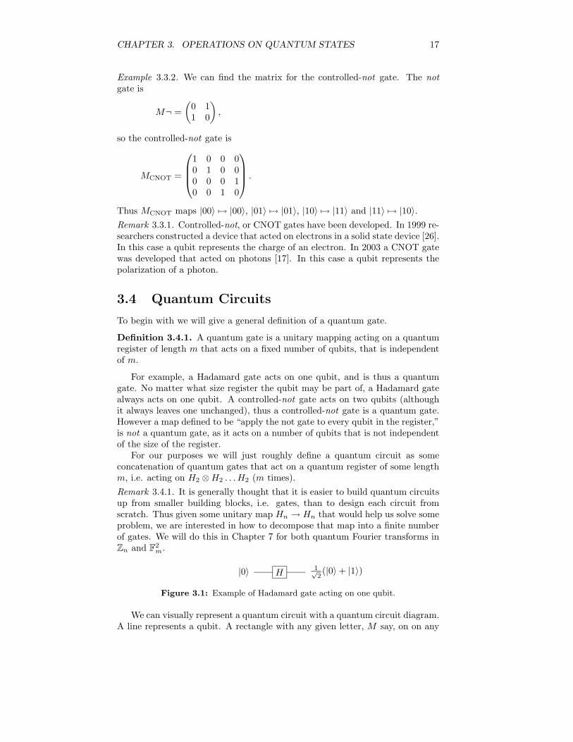
Example 3.3.2. We can find the matrix for the controlled-not gate. The notgate is

M¬ =

(0 11 0

),

so the controlled-not gate is

MCNOT =

1 0 0 00 1 0 00 0 0 10 0 1 0

.

Thus MCNOT maps |00〉 7→ |00〉, |01〉 7→ |01〉, |10〉 7→ |11〉 and |11〉 7→ |10〉.Remark 3.3.1. Controlled-not, or CNOT gates have been developed. In 1999 re-searchers constructed a device that acted on electrons in a solid state device [26].In this case a qubit represents the charge of an electron. In 2003 a CNOT gatewas developed that acted on photons [17]. In this case a qubit represents thepolarization of a photon.

3.4 Quantum Circuits

To begin with we will give a general definition of a quantum gate.

Definition 3.4.1. A quantum gate is a unitary mapping acting on a quantumregister of length m that acts on a fixed number of qubits, that is independentof m.

For example, a Hadamard gate acts on one qubit, and is thus a quantumgate. No matter what size register the qubit may be part of, a Hadamard gatealways acts on one qubit. A controlled-not gate acts on two qubits (althoughit always leaves one unchanged), thus a controlled-not gate is a quantum gate.However a map defined to be “apply the not gate to every qubit in the register,”is not a quantum gate, as it acts on a number of qubits that is not independentof the size of the register.

For our purposes we will just roughly define a quantum circuit as someconcatenation of quantum gates that act on a quantum register of some lengthm, i.e. acting on H2 ⊗H2 . . .H2 (m times).

Remark 3.4.1. It is generally thought that it is easier to build quantum circuitsup from smaller building blocks, i.e. gates, than to design each circuit fromscratch. Thus given some unitary map Hn → Hn that would help us solve someproblem, we are interested in how to decompose that map into a finite numberof gates. We will do this in Chapter 7 for both quantum Fourier transforms inZn and F2

m.

|0〉 H1√2(|0〉+ |1〉)

Figure 3.1: Example of Hadamard gate acting on one qubit.

We can visually represent a quantum circuit with a quantum circuit diagram.A line represents a qubit. A rectangle with any given letter, M say, on on any


number of lines, represents the action of the gate M on the qubits representedby the lines. Inputs are on the left, and outputs on the right. Figure 3.1represents a circuit of just one gate, the Hadamard gate H, acting on a qubitwith initial state |0〉. However for the not gate we use a slightly different visualrepresentation, as can be seen in Figure 3.2. As in Figure 3.3, a controlled

|0〉 �� |1〉

Figure 3.2: Example of a not gate acting on one qubit.

gate is shown with a filled black circle on the control qubit, and the ordinarysymbol for the gate on the target qubit, with a line connecting the two. For a

|1〉 • |1〉

|0〉 �� |1〉

Figure 3.3: Example of a controlled-not gate.

measurement we will use a ‘tab’ symbol containing an M , and for qubits thatare definitely in pure states, (or equivalently classical bits) we use a ‘double

1√2

(|0〉+ |1〉) "%#$M ?

Figure 3.4: Example of a measurement. Note that for the input mixed state1

√

2(|0〉 + |1〉), it is unknown what the result of the measurement will be. All that

is known is that the result has equal probability of being |0〉 or |1〉.

line’ as in Figure 3.4. We also have two important theorems relating to theconstruction of quantum circuits, which we leave unproved.

Theorem 3.4.1 ([1]). All quantum circuits can be constructed using only con-trolled not and unary gates.

Theorem 3.4.2 ([20]). All quantum circuits can be constructed (in some ap-proximated sense) using only Hadamard gates and Toffoli gates.

A Toffoli gate is a three qubit gate that we will define in the next chapter.

Chapter 4

Boolean Circuits

We may wish to implement some classical operation using quantum gates thatdoes not seem correspond to any unitary map. The map that the circuit in

Cx ∈ F2n f(x) ∈ F2

m

Figure 4.1: Boolean circuit performing function f : F2

n→ F2

m.

Figure 4.1 performs cannot be a unitary operation (if we take the input andoutput to be some quantum registers in a pure state). The number of inputsdo not equal the number of outputs, so the map is not invertible. This chaptershows how given any classical boolean circuit, it is in fact possible to constructa quantum circuit that performs the same function.

4.1 Boolean Circuits

For our purposes we say that a classical bit is essentially the same as a quantumbit, but that the state of a classical bit must always be a pure state, i.e. either|0〉 or |1〉. There are three boolean gates, i.e. 3 gates that act on the pure states|0〉 and |1〉, and output one of the pure states |0〉 or |1〉. They are the and (∧),or (∨) and the not (¬) gates.

A boolean circuit is some combination of these gates, and the fanout oper-ation, where the output of one gate is essentially copied and used as the inputto several other gates.

19

CHAPTER 4. BOOLEAN CIRCUITS 20

|x〉 |y〉 |x ∧ y〉 (and) |x ∨ y〉 (or) |¬x〉 (not)|0〉 |0〉 |0〉 |0〉 |1〉|0〉 |1〉 |0〉 |1〉 |1〉|1〉 |0〉 |0〉 |1〉 |0〉|1〉 |1〉 |1〉 |1〉 |0〉

Figure 4.2: Truth table for boolean gates and, or and not.

We consider |0〉 and |1〉 as representing members of a group, specifically |0〉represents 0 ∈ F2 and |1〉 represents 1 ∈ F2 (cf Section 2.4). We also say thata basis vector |x0〉 |x1〉 . . . |xm−1〉 in the compound system H2 ⊗ . . . ⊗ H2 (mtimes) represents the element (x0, x1, . . . , xm−1) ∈ Fm

2 . Thus we can say that aboolean circuit actually performs a function Fn

2 → Fm2 .

Let us consider functions Fn2 → Fm

2 . In 1941 Emil Post [18]1 proved that anysuch function can be constructed using only the three boolean gates and, or andnot (and fanout), and thus a boolean circuit can be constructed to perform thisfunction. Thus if we can find unitary gates that perform these functions, we canshow that given any function Fn

2 → Fm2 , a quantum circuit can be constructed

that performs it.The important gate that we will use is the Toffoli gate. It acts on three

qubits and maps |x〉 |y〉 |z〉 → |x〉 |y〉 |x⊕ (y ∧ z〉 where ∧ is and and ⊕ exclusiveor (or in other words addition modulo two). It can itself be constructed usingHadamard gates, controlled phase flip gates and controlled-not gates as shownin Figure 4.4. The symbol for Toffoli gate is shown in Figure 4.3. We will

|x〉 • |x〉

|y〉 • |y〉

|z〉 �� |x⊕ (y ∧ z〉)

Figure 4.3: Toffoli gate.

|x〉 • • • |x〉

|y〉 • �� • �� |y〉

|z〉 H Fπ/2 F3π/2 Fπ/2 H |x⊕ (y ∧ z〉)

Figure 4.4: Decomposition of a Toffoli gate.

now describe how quantum gates can be used to perform the same function asboolean gates.

1According to [11]. Unfortunately a copy of [18] was not found.


1. And An and gate can be constructed using a Toffoli gate as in Figure 4.5.Note that an additional qubit is required in pure state |0〉, which we willcall an ancilla qubit.

|x〉 • |x〉|y〉 • |y〉

|0〉 �� |x ∧ y〉

Figure 4.5: Toffoli gate as an and gate.

2. Not As shown in the previous chapter, a not gate is already unitary.

3. Or An or gate can be constructed using an and gate and three not gates.Thus it can be constructed with a Toffoli gate, three not gates and requiresan ancilla qubit in pure state |0〉 as in Figure 4.6.

|x〉 �� • |¬x〉

|y〉 �� • |¬y〉

|0〉 �� |x ∨ y〉

Figure 4.6: A Toffoli gate as an or gate.

4. Fanout A fanout can be constructed using a Toffoli gate and one notgate. Note we need two ancilla qubits to achieve this, both in pure state|0〉. As can be seen in Figure 4.7, technically we could omit the not gateand have one of the ancilla qubits initially in state |1〉, but it is easier totreat all ancilla qubits as having to be in state |0〉. We can see that thismap actually copies basis states. We cannot have a unitary map that willcopy all mixed states, as we will see in Chapter 6.

|x〉 • |x〉

|0〉 �� • |1〉

|0〉 �� |x〉

Figure 4.7: Toffoli gate as fanout.


Thus given any boolean circuit that computes a function f : F2n → F2

m with kgates we can construct a quantum circuit, R, that performs the same function.The quantum circuit uses O(k) gates2 and requires q = O(k) ancilla qubits, allinitially in pure state |0〉. Such a circuit would also output m+ n− q ‘garbagequbits’, and is shown in Figure 4.8.

R

|f(x)〉

|x〉

garbage bits

|0〉 (ancilla qubits)

Figure 4.8: Quantum circuit emulating boolean circuit that performs functionf : F2

n→ F2

m.

However the garbage qubits may be undesirable. Since R is a quantumcircuit it has an inverse R−1. In fact, the Toffoli and not gates are self inverse,so we can just take the ‘mirror image’ of the circuit R for R−1. Using this and acollection of controlled-not gates we can construct the following quantum circuitthat requires the presence of ancilla bits, all initially in state |0〉, but outputsthem all in state |0〉 (perhaps to be used again). One feature of this circuit isthat the input is preserved, perhaps to be used in some other circuit. Such acircuit is shown in Figure 4.9.

2For functions f, g : N → N we say f = O(g) if there are constants c > 0 and n0 ∈ N suchthat n > n0 implies f(n) ≤ cg(n).


R

•

R−1

••••••|x〉 • |x〉

|0〉 |0〉

��|0〉 �� |f(x)〉

��

Figure 4.9: Quantum circuit emulating boolean circuit that performs functionf : F2

n→ F2

m. Note that this circuit preserves input and ancilla qubits.

Chapter 5

Superdense Coding

In this chapter we will describe a simple algorithm by which two classical bitsof information can be encoded into one qubit, the qubit transmitted, and theoriginal two classical bits recovered [4]. As is traditional, the sender is calledAlice, and the receiver is called Bob.

For this, we assume that Alice and Bob have a quantum channel: somemeans of Alice to transmit a qubit to Bob. We also assume that Alice and Bobshare an entangled pair of qubits in state

1√2(|00〉+ |11〉).

Alice’s qubit is on the left in the above expression, which we will label A, andBob’s qubit is on the right, which we will label B. One could say that for Aliceand Bob to share this EPR pair, they needed to have previously transmitteda qubit. However no transmission of the classical bits occurs at this point, asAlice may not have even decided what classical bits she will send to Bob whenthis initial transmission occurs.

We will label Alice’s classical bits as a and b. Note that these are the sameas quantum bits in pure states |a〉 and |b〉 respectively. The protocol follows.

1. If a = 1 Alice performs the phase flip F on her qubit A.

a State after Alice’s first operation0 1√

2(|00〉+ |11〉)

1 1√2(|00〉 − |11〉)

2. If b Alice also performs the not operation on her qubit A.

a b State after Alice’s second operation0 0 1√

2(|00〉+ |11〉)

0 1 1√2(|10〉+ |01〉)

1 0 1√2(|00〉 − |11〉)

1 1 1√2(|10〉 − |01〉)

3. Alice transmits her qubit to Bob.

24

CHAPTER 5. SUPERDENSE CODING 25

4. Bob performs the controlled-not on his qubit B using the qubit A as thecontrol qubit.

a b State after Bob’s first operation0 0 1√

2(|00〉+ |10〉)

0 1 1√2(|11〉+ |01〉)

1 0 1√2(|00〉 − |10〉)

1 1 1√2(|11〉 − |01〉)

5. Bob performs the Hadamard Transform H on A. At this point the qubitsare guaranteed to be in state |ab〉.

6. Bob observes the two qubits A and B. He is certain of observing a and b.

Note that this process has copied the classical bits a and b. Both Alice andBob each have a copy of a and b at the end of this protocol. Since we can viewclassical bits as quantum bits in pure states, this process has essentially copiedtwo pure quantum states. It is impossible to copy a general mixed state usingunitary maps, as will be proved in the next chapter.

Alice

a • a

b • b

A F ��

Bob

• H "%#$M a

B �� "%#$M b

Figure 5.1: Superdense coding.

Chapter 6

Quantum Teleportation

In this chapter we will describe the converse to superdense coding: how the stateof a qubit can somehow be ‘encoded’ into two classical bits, the bits transmitted,and the original state recovered. As in the previous chapter the sender with theoriginal state to send is called Alice, and the receiver Bob. This protocol wasintroduced in [3].

For this we will assume that Alice and Bob have a classical channel: somemeans for Alice to send classical bits to Bob.

Remark. A classical channel is any traditional means of sending information:fax, e-mail - even carrier pigeon!

Remark. Quantum teleportation has been successfully carried out a numberof times, teleporting states of atoms or photons. Most notably was a 600mteleportation of photons across the River Danube, Vienna Austria in 2004 [22].We will not discuss the issue in any depth, but quantum teleportation is crucialin quantum communication schemes.

Also as before we will start with Alice and Bob sharing an EPR pair

1√2(|00〉+ |11〉). (6.1)

One could say that to get to this point that Alice and Bob had to share aquantum channel. However, this could have happened a long time before Alicehad the qubit to teleport to Bob.

One very important point to make is that this process teleports the quantumstate. The encoding process actually destroys the original quantum state. Thereis actually no way to copy a general quantum state using unitary mappings aswe will see later in this chapter.

In the EPR pair (6.1), Alice has the qubit on the left which we will label A,and Bob has the qubit on the right which we will call B. Alice’s qubit to beteleported we will label T . It is in (possibly) a mixed state which we will referto as |ψ〉 = a |0〉+ b |1〉 for some unknown a, b ∈ C where |a|2 + |b|2 = 1. Thusthe compound state of the system T ⊗A⊗B is

(a |0〉+ b |1〉) 1√2(|00〉+ |11〉)

=a√2|000〉+ a√

2|011〉+ b√

2|100〉+ b√

2|111〉 .

26

CHAPTER 6. QUANTUM TELEPORTATION 27

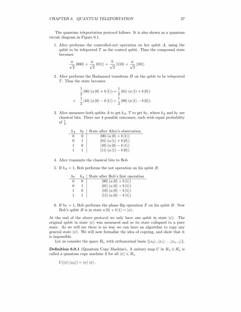
The quantum teleportation protocol follows. It is also shown as a quantumcircuit diagram in Figure 6.1.

1. Alice performs the controlled-not operation on her qubit A, using thequbit to be teleported T as the control qubit. Thus the compound statebecomes

a√2|000〉+ a√

2|011〉+ b√

2|110〉+ a√

2|101〉

2. Alice performs the Hadamard transform H on the qubit to be teleportedT . Thus the state becomes

1

2|00〉 (a |0〉+ b |1〉) +

1

2|01〉 (a |1〉+ b |0〉)

+1

2|10〉 (a |0〉 − b |1〉) +

1

2|00〉 (a |1〉 − b |0〉).

3. Alice measures both qubits A to get bA, T to get bT , where bA and bT areclassical bits. There are 4 possible outcomes, each with equal probabilityof 1

4 .

bA bT State after Alice’s observation0 0 |00〉 (a |0〉+ b |1〉)0 1 |01〉 (a |1〉+ b |0〉)1 0 |10〉 (a |0〉 − b |1〉)1 1 |11〉 (a |1〉 − b |0〉)

4. Alice transmits the classical bits to Bob

5. If bA = 1, Bob performs the not operation on his qubit B.

bT bA State after Bob’s first operation0 0 |00〉 (a |0〉+ b |1〉)0 1 |01〉 (a |0〉+ b |1〉)1 0 |10〉 (a |0〉 − b |1〉)1 1 |11〉 (a |0〉 − b |1〉)

6. If bT = 1, Bob performs the phase flip operation F on his qubit B. NowBob’s qubit B is in state a |0〉+ b |1〉 = |ψ〉.

At the end of the above protocol we only have one qubit in state |ψ〉. Theoriginal qubit in state |ψ〉 was measured and so its state collapsed to a purestate. As we will see there is no way we can have an algorithm to copy anygeneral state |ψ〉. We will now formalise the idea of copying, and show that itis impossible.

Let us consider the space Hn with orthonormal basis {|x0〉 , |x1〉 . . . |xn−1〉}.

Definition 6.0.1 (Quantum Copy Machine). A unitary map U in Hn ⊗Hn iscalled a quantum copy machine if for all |ψ〉 ∈ Hn

U(|ψ〉 |x0〉) = |ψ〉 |ψ〉 .

CHAPTER 6. QUANTUM TELEPORTATION 28

Alice

|ψ〉 • H "%#$M

A �� "%#$M

Bob

••

B �� F |ψ〉

Figure 6.1: Quantum teleportation.

Using this definition we now give the following result [25].

Theorem 6.0.1 (No-Cloning Theorem). For n > 1 there does not exist aquantum copy machine.

Proof. Let us assume that n > 1 and that a quantum copy machine, U , exists.Since n > 1 there must be two orthonormal basis vectors |x0〉 and |x1〉. Let|ψ〉 = 1√

2(|x0〉+ |x1〉). Thus by definition of quantum copy machine

U (|ψ〉 |x0〉) = |ψ〉 |ψ〉

=1

2(|x0〉 |x0〉+ |x0〉 |x1〉+ |x1〉 |x0〉+ |x1〉 |x1〉) .

However U is linear so

U(|ψ〉 |x0〉) = U

(1√2

(|x0〉+ |x1〉) |x0〉)

=1√2U(|x0〉 |x0〉) +

1√2U(|x1〉 |x0〉)

=1√2|x0〉 |x0〉+

1√2|x1〉 |x1〉

This is a contradiction.

Thus by the No-Cloning Theorem there does not exist any combination ofunitary maps so that an arbitrary quantum state can be copied. Note howeverthat the No-Cloning Theorem does not forbid a combination of unitary mapsin Hn ⊗Hn to copy basis states. In fact we have already seen two examples ofthis: superdense coding and the use of the Toffoli gate for fanout of classicalbits (remember that a classical bit is essentially the same as quantum bit in apure state).

Chapter 7

Quantum FourierTransform

In this chapter we investigate an important map of quantum systems, the quan-tum Fourier transform. As we will see this map is a unitary linear map, andwe shall find how to decompose it into a finite number of quantum gates. Thismap is used in all of the following chapters describing quantum algorithms.

7.1 Discrete Fourier Transform

We will in this section extremely briefly, and largely without proof, describewhat we mean by characters and discrete Fourier transform. Throughout thischapter G will be a finite abelian group, and n = |G|. We will also say G ={g1, g2, . . . , gn}. The group operation in G will be written additively.

7.1.1 Characters of Finite Abelian Groups

Definition 7.1.1. A character of G is a homomorphism χ : G→ C\{0}.

Note that for all g ∈ G and characters χ of G, χ(g) is an nth root of unity.Since χ is a homomorphism and ng = 1G, we have χ(g)n = χ(ng) = χ(1G) = 1.

We can see that the characters themselves form an abelian group, with theproduct (we will use multiplicative notation) of two characters χα and χβ isdefined by requiring it to satisfy χαχβ(g) = χα(g)χβ(g) for all g in G. We call

this group either the character group or the dual group of G, and write it as G.We then have the following result, which we state without proof.

Lemma 7.1.1. Let G be a finite abelian group. Then G ∼= G.

One thing the above lemma implies is that there are exactly the same numberof characters as elements of the group, i.e. there is a one to one correspondencebetween the two. Let us consider the cyclic group Zn. For each fixed y ∈ Zn

define χy by

χy(x) = e2πixy

n .

29

CHAPTER 7. QUANTUM FOURIER TRANSFORM 30

There is a one to one correspondence between Zn and all the characters of Zn.Therefore each character of Zn is equal to χy for some unique y ∈ Zn.

We can also find the characters of Fm2 . We know that

Fm2 = F2 ⊕ F2 ⊕ · · · ⊕ F2 (m times). (7.1)

Lemma 7.1.1 shows that the character group of Fm2 must be isomorphic to Fm

2

itself. Thus by equation (7.1) each character of Fm2 must be equal to the product

of m characters of F2, and given m characters of F2 their product must be equalto a character of Fm

2 . Now note that F2∼= Z2. Each character of Z2 is given by,

for some y ∈ Z2,

χy(x) = e2πixy

n = (−1)xy.

The decomposition (7.1) means that for each x ∈ Fm2 there are xi ∈ F2 such

that x = (x1, x2, . . . , xm). Therefore each character of Fm2 is determined by

y ∈ Fm2 so that

χy(x) = (−1)x.y,

where . is the standard inner product.

7.1.2 Discrete Fourier Transform

Let us consider the vector space V of functions f : G→ C. We assign to V aninner product defined by

〈f1|f2〉 =n∑

k=1

f∗1 (gk)f2(gk).

It can be shown that the set{

1√nχ1,

1√nχ2, . . . ,

1√nχn

},

is a basis of this space, which we will call the character basis. Therefore foreach function f : G → C there exist (unique) coefficients fi ∈ C, the fouriercoefficients, such that

f = f11√nχ1 + f2

1√nχ2 + . . .+ fn

1√nχn.

Definition 7.1.2. Given a function f : G→ C, the discrete Fourier transformof f is the function f : G→ C defined by

f(gi) = fi,

where fi is defined above.

Given the values of f(gi) and the character of the group χi there is an easyway to find the Fourier transform (which can be easily derived using the fact


that the characters form a basis of the space, and so must be orthogonal withrespect to the inner product). We have

f(gi) =1√n

n∑

k=1

χ∗i (gk)f(gk).

Because we have found all of the characters of Fm2 and Zn, we can simply

substitute them into the above equation to find the Fourier transform for anyfunctions Fm

2 → C and Zn → C. Let f : Zn → C. Then the Fourier transformof f is

f(x) =1√n

∑

y∈Zn

e−2πixy

n f(y).

Let f : Fm2 → C. Then the Fourier transform of f is

f(x) =1√2m

∑

y∈F2n

(−1)x.yf(y).

There is also an inverse to the Fourier transform, which we now define.

Definition 7.1.3. Given a function f : G→ C, the inverse Fourier transformof f is defined to be the function f : G→ C

f(gi) =1√n

n∑

k=1

χk(gi)f(gk).

If we consider both the forward and inverse transforms for all gi and writethem out as matrix vector equations, we can see that

f =

˜f.

We can see that the inverse Fourier transform in Zn looks very similar to theforward transform

f(x) =1√n

∑

y∈Zn

e2πixy

n f(y).

The inverse transform in Fm2 is exactly equal to the forward transform, i.e. it is

self inverse.We also have an identity that is very important. This will be used to show

the quantum Fourier transform, that we will define later, is a unitary map.We define the norm on V by ‖f‖ =

√〈f |f〉. We leave the following theorem

unproved.

Theorem 7.1.1 (Pareseval’s Identity).

‖f‖ = ‖f‖

It should be noted that Fourier transforms are known to be able to ‘extract’the periods of functions. We use this fact in Chapter 9 to factor integers.


7.2 Quantum Fourier Transform

Let G = {g1, g2, . . . , gn} be a finite abelian group, and let {χ1, χ2, . . . , χn} bethe set of characters of G. We will also let Hn be an n-dimensional quantumsystem. We label an orthogonal basis of Hn by {|g1〉 , |g2〉 , . . . , |gn〉}. Thus wesay that Hn represents G (see section 2.4).

We also note that any quantum state

n∑

i=1

αi |gi〉 wheren∑

i=1

|αi|2 = 1 (7.2)

defines a map

f : G→ C with f(gi) = αi and ‖f‖ = 1. (7.3)

We can see that given map of the form of (7.3) defines a quantum state of theform of (7.2). Thus a general quantum state can be written as

n∑

i=1

f(gi) |gi〉 where f : G→ C and ‖f‖ = 1. (7.4)

Definition 7.2.1. The quantum Fourier transform (QFT ) in G is the map onHn defined by

n∑

i=1

f(gi) |gi〉QFTG7−−−−→

n∑

i=1

f(gi) |gi〉 , (7.5)

where f is the ordinary discrete Fourier transform of f .

Lemma 7.2.1. The quantum Fourier transform is a unitary map on Hn.

Proof. It is clear by the definition that the quantum Fourier transform is linear.By Parseval’s identity 7.1.1 we have that ‖f‖ = ‖f‖. Thus Fourier transformis a norm preserving linear map on a finite dimensional Hilbert space, and somust be unitary.

Recall that the Fourier transform of f is

f =1√n

n∑

i=1

χ∗i (gi)f(gi),

so for basis vectors |gi〉 the QFT is

|gi〉QFTG7−−−−→ 1√

n

n∑

i=1

χ∗i (gi) |gi〉 . (7.6)

Since QFT is linear if we find a linear map that performs the above operationon basis states |gi〉, then it would perform the general QFT (7.5) on generalmixed states.

It should be noted that the QFT depends on the group G. If we took thatHn represents some other group, then the Fourier transform of that group wouldbe different, and so the quantum Fourier transform on Hn would be different.We use QFT when we take Hm to represent either Fm

2 or Z2m .


7.2.1 Quantum Fourier Transform in Fm2

From Section 7.1.1 we see that the characters of Fm2 are χy(x) = (−1)x.y. Thus

if we label an orthonormal basis of H2m as {|x〉 : x ∈ Fm2 } the QFT in Fm

2 onH2m on a basis vector is

|x〉QFTF

m27−−−−−→ 1√

2m

∑

y∈Fm2

(−1)x.y |y〉 . (7.7)

We recall that H2m is a quantum register of length m. That is, the compoundsystem of m qubits. We can show this in general circuit diagram Figure 7.1.Note that technically the diagram does not show describe a quantum circuit.A quantum circuit is defined to be some collection of quantum gates, and aquantum gate is defined to act on some finite number of qubits that is indepen-dent of the size of the register. However, we can, and will now, decompose this

QFTFm2

|x〉 1√2m

∑

y∈Fm2

(−1)x.y |y〉

......

Figure 7.1: Quantum Fourier transform in Fm

2 .

transform into some finite number of quantum gates.Let us first consider a more general case. Let G be a finite abelian group

such that G = U⊕V . Let U = {u1, u2, . . . , us} and V = {v1, v2, . . . , vs}. Let Hr

represent U and Hs represent V . By this we mean that we label an orthonormalbasis of Hr by {|u1〉 , |u2〉 , . . . , |ur〉} and we label an orthonormal basis of Hs

by {|v1〉 , |v2〉 , . . . , |vs〉}. Since G = U ⊕ V all members of G can be uniquelyexpressed as gij = ui + vj . Thus the vector |ui〉 |vj〉 ∈ Hr ⊗Hs = Hrs can bethought of as representing the unique gij such that gij = ui + vj , so we define|gij〉 = |ui〉 |vj〉 . Thus Hrs represents G.

By Lemma 7.1.1 we can know that G = U ⊗ V . Thus any character of Gcan be uniquely written as χkl(gij) = χU

k (ui)χVl (vj), for characters χU

k and χVl

of U and V respectively. -

Lemma 7.2.2. Using the above notation, the map

|gij〉 7−→( 1√

r

r∑

k=1

(χUk (ui))

∗ |uk〉)( 1√

s

s∑

l=1

(χVl (vj))

∗ |vl〉)

is the QFT in G on Hrs.


Proof. If we expand out the RHS using the definition of tensor product, we get

RHS =( 1√

rs

r∑

k=1

s∑

l=1

(χUk (ui))

∗(χVl (vi))

∗ |uk〉 |vl〉)

=( 1√

rs

r∑

k=1

s∑

l=1

χ∗kl(ui + uj) |uk + vl〉

)

=( 1√

rs

r∑

k=1

s∑

l=1

χ∗kl(gij) |gij〉

),

Which is exactly the quantum Fourier transform of in G of |gij〉.

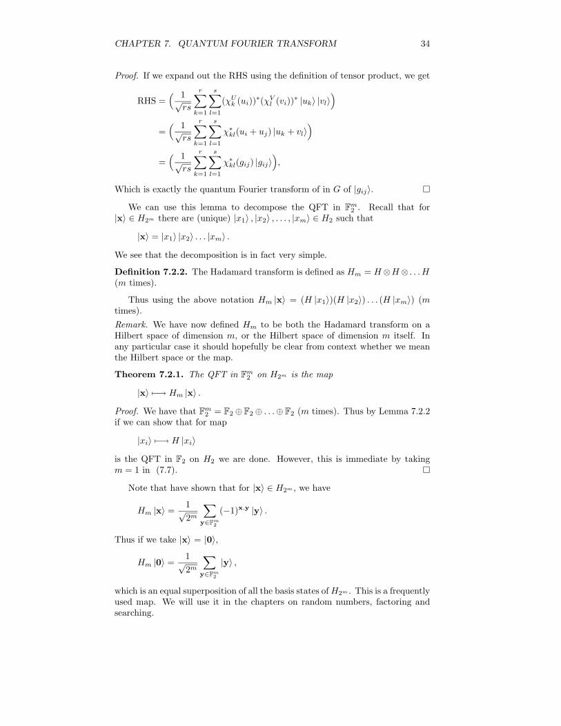
We can use this lemma to decompose the QFT in Fm2 . Recall that for

|x〉 ∈ H2m there are (unique) |x1〉 , |x2〉 , . . . , |xm〉 ∈ H2 such that

|x〉 = |x1〉 |x2〉 . . . |xm〉 .

We see that the decomposition is in fact very simple.

Definition 7.2.2. The Hadamard transform is defined as Hm = H⊗H⊗ . . .H(m times).

Thus using the above notation Hm |x〉 = (H |x1〉)(H |x2〉) . . . (H |xm〉) (mtimes).

Remark. We have now defined Hm to be both the Hadamard transform on aHilbert space of dimension m, or the Hilbert space of dimension m itself. Inany particular case it should hopefully be clear from context whether we meanthe Hilbert space or the map.

Theorem 7.2.1. The QFT in Fm2 on H2m is the map

|x〉 7−→ Hm |x〉 .

Proof. We have that Fm2 = F2⊕F2⊕ . . .⊕F2 (m times). Thus by Lemma 7.2.2

if we can show that for map

|xi〉 7−→ H |xi〉

is the QFT in F2 on H2 we are done. However, this is immediate by takingm = 1 in (7.7).

Note that have shown that for |x〉 ∈ H2m , we have

Hm |x〉 =1√2m

∑

y∈Fm2

(−1)x.y |y〉 .

Thus if we take |x〉 = |0〉,

Hm |0〉 =1√2m

∑

y∈Fm2

|y〉 ,

which is an equal superposition of all the basis states ofH2m . This is a frequentlyused map. We will use it in the chapters on random numbers, factoring andsearching.


H

H

|x〉H

1√2m

∑

y∈Fm2

(−1)x.y |y〉

......

H

Figure 7.2: Decomposition of QFT in Fm

2 .

7.2.2 Quantum Fourier Transform in Zn

From Section 7.1.1 we know that the characters of Zn are of the form χy(x) =

e2πxy

n . Recall also from section 2.4 that if n = 2m then Zn can be very naturallyrepresented by H2m (i.e. m qubits). That is, given x ∈ Z2m , we see that thereare xi ∈ {0, 1} such that

x = 2m−1xm−1 + 2m−2xm−2 + . . .+ 2x1 + x0.

Thus we define |x〉 to be |xm−1〉 |xm−2〉 . . . |x0〉 and say that |x〉 represents x.We will actually be working with the inverse quantum Fourier transform. Wedo this for two reasons. Firstly in the next chapter, Shor’s algorithm uses theinverse quantum Fourier transform. Secondly it is ever so slightly less confusingworking with the inverse transform (as there are less ‘−’s in our expressions).However, the expressions are all very similar for the forward transform - it shouldnot be too difficult to do though all the stages of the decomposition, puttingin ‘−’s where appropriate to get the decomposition for the forward quantumFourier transform.

By Section 7.1.2 we know that the inverse quantum Fourier transform inZ2m on H2m is the map

|x〉QFT−1

Zn7−−−−−→ 1√2m

2m−1∑

y=0

e2πxy2m |y〉

We know that this is linear, and unitary, but we would like to be able to de-compose it to some finite number of quantum gates. We will use the followingtwo lemmata

Lemma 7.2.3.

2m−1∑

y=0

e2πxy2n |y〉 = (|0〉+ e

πix

20 |1〉)(|0〉+ eπix

21 |1〉) . . . eπix

21 |m− 1〉) (7.8)

Proof. Note for each y ∈ Z2m there are yi ∈ {0, 1} such that

y = 2m−1ym−1 + 2m−2ym−2 + . . .+ 2y1 + y0.

For each y ∈ Z2m let y′ ∈ Z2m−1 such that

y′ = 2m−2ym−1 + 2m−3ym−2 + . . .+ 1y1,


so y = 2y′ + y0. Thus we can split up the sum

2m−1∑

y=0

e2πxy2n |y〉 =

2m−1−1∑

y′=0

e2πix(2y′+0)

2m |2y′ + 0〉+2m−1−1∑

y′=0

e2πix(2y′+1)

2m |2y′ + 1〉

=2m−1−1∑

y′=0

e2πix2y′

2m |y′〉 |0〉+2m−1−1∑

y′=0

e2πix2y′

2m e2πix2m |y′〉 |1〉

=2m−1−1∑

y′=0

e2πixy′)

2m−1 |y′〉 (|0〉+ eπix

2m−1 |1〉)

We can continue applying the same method to the sum on the RHS.

Lemma 7.2.4. Let x ∈ Z2m , with xi ∈ {0, 1} such that

x = 2m−1xm−1 + 2m−2xm−2 + . . .+ 2x1 + x0.

Then

exp(πix

2l−1) = (−1)xl−1 exp(

πixl−2

21) . . . exp(

πix1

2l−2) exp(

πix0

2l−1)

Proof.

exp(πix

2l−1) = exp(

πi(2m−1xm−1 + 2m−2xm−2 + . . .+ 2x1 + x0)

2l−1)

= exp(πi(2l−1xl−1 + 2l−2xl−2 + . . .+ 2x1 + x0)

2l−1)

(since exp is 2π-periodic)

= (−1)xl−1 exp(πixl−2

21) . . . exp(

πix1

2l−2) exp(

πix0

2l−1)

Using these two lemmata we can show how to compute the quantum Fouriertransform in Z2m on H2m . Firstly we swap the order of the qubits, so

|xm−1〉 |xm−2〉 . . . |x1〉 |x0〉 7−→ |x0〉 |x1〉 |xm−2〉 |xm−1〉

A swap of the state of two qubits can be achieved by three controlled-not gates,as in Figure 7.3. Now what we want to do is to apply unitary maps on the

|ψ〉 • �� • |φ〉|φ〉 �� • �� |ψ〉

Figure 7.3: Swap of two qubits.

qubits so that the expression has the form given by equation (7.8), multipliedby a factor 1/

√2m. This means that for the lth qubit from the left we want

the coefficient of |0〉 to be 1/√

2m and the coefficient of |1〉 to be (1/√

2m)eπix

2l−1 .Let us label the qubits from left to right as A0, A1, . . . , Am−1. We perform thefollowing steps for l = m− 1 . . . 1 (in this order)

1. Notice qubit Al is in state |xl〉.


2. We apply the Hadamard Walsh gate to Al, so

|xl〉 7−→1√2(|0〉+ ((−1)xl |1〉)

3. For each k = l . . . 0 apply to Al the phase flip φlk defined as

φlk = F π

2l−k=

(1 0

0 eπi

2l−k

)

but controlled with the control qubit Ak.

4. By Lemma (7.2.4) qubit Al is now in state.

1√2(|0〉+ e

πix

2l−1 |1〉)

Once all these steps are completed, by Lemma (7.8) the QFT in Z2m has beenperformed. A circuit diagram for these steps is shown in Figure 7.4 (the swap-ping of the bits has been omitted, as have the subscripts for φ).

|xm−1〉 H φ φ φ |y0〉

|xm−2〉 • H φ φ |y1〉

|xm−3〉 • • H φ |y2〉...

. . .. . .

. . ....

|x0〉 • • • H |ym−1〉

Figure 7.4: Decomposition of QFT in Z2m .

Chapter 8

Random Numbers

Random numbers are quite useful in various computer calculations. For exam-ple they can assist is finding large multidimensional integrals, or in optimizationprocesses using Monte Carlo methods. Random numbers produced on a stan-dard computer are not really random, they are pseudorandom. They are deter-ministic - you put in the same input, i.e. the seed, and the generator will returnthe same output every time. This means that there is an underlying pattern tothe numbers produced. This pattern may be subtle, but it still adversely affectsthe algorithms that require random numbers.

There are commercially available devices to generate random numbers thatexploit quantum effects, such as the chance that a photon will go through asemi-silvered mirror, or the decay time for some radioactive isotope. Howeverit is interesting to see how a quantum circuit could be constructed to generaterandom numbers. We will see that we already have already discussed all therequired tools to do so.

Let us take Hm to represent Z2m . We start with m qubits in state

|0〉

and then apply the Hadamard transform Hm to get

1√2m

2m−1∑

i=0

|i〉 .

We then measure the system. Each integer in the range 0 . . . 2m−1 is measuredwith equal probability. Specifically, each is measured with probability 1/

√2m.

Hm M

=<

:;

|0〉 |y〉...

...

Figure 8.1: Circuit that generates random numbers.

38

Chapter 9

Factoring

In this chapter we show that quantum circuits offer us a way to factor largeintegers, a problem that was previously thought to be more or less unfeasible.

9.1 One Way Functions

Although not proved, multiplication is believed to be a one way function.Roughly speaking, a one way function is one that easy to compute but hardto compute the inverse.

By easy we generally mean that there is an algorithm that perform a numberof operations that is equal to (or less than) some polynomial function of theinput size. If n is the input size, then we say the number of operations is equalto O(nk) for some fixed k. We also will call such functions efficient. By hardwe can mean that an efficient (classical) algorithm doesn’t exist. That any oneway functions actually exist is an open problem.

x f(x)

HARD

easy

Figure 9.1: A one-way function

It is generally believed that multiplication is a one way function, i.e. theredoes not exist an efficient (classical) algorithm that factors integers. The fastestalgorithms known scale in complexity (i.e. the number of operations required)with respect to some exponential function of the input size. Current popular

39

CHAPTER 9. FACTORING 40

encryption algorithms such as RSA are seen as secure as it is assumed thatmultiplication is a one way function. Roughly speaking authorized viewers datacan decrypt data because they know the correct factors of some number tomultiply together to obtain the decryption key. Unauthorized eavesdroppersdo not know all the factors, and so would have to calculate them themselves.For large numbers this would take a very long time on current computers. Forexample current classical computers would take several million years to factora 256 digit number.

Shor’s algorithm [21] gives us a way to factor these integers using quantumcircuits. This algorithm is not deterministic, and will not output a factor everytime, but it will output a factor with high enough probability so that if it isrun enough times, it would find a factor on average with fewer operations thana current classical computer.

Remark 9.1.1. Shor’s algorithm has been implemented in an NMR quantumcomputer, but the most only to factor 15 into 3 and 5 using a 7 qubit [23].

Remark. This chapter contains several purely number theoretical results. Theproofs to these are often omitted. Unless otherwise stated, the proofs can befound in [11].

9.2 Factors from Order

In this section will show that factoring a number n can be reduced to finding theorder of an element in a ∈ Z∗

n. Recall that Z∗n is the group of integers modulo

n with the group operation multiplication (and so must have a multiplicativeinverse).

Lemma 9.2.1. Z∗n contains exactly all those a in a ∈ Zn such that gcd(a, n) =

1.

For the sake of brevity throughout this chapter a will be a member of Z∗n

and r will be the order of a in Z∗n. Thus r is the smallest integer such that

ar ≡ 1 mod n. (9.1)

Note for any finite group G, and for any g ∈ G we have g|G| = 1G. Thus r ≤ n.Also note that if n is a power of a single prime, there do exist efficient classicalalgorithms that can determine whether this is the case and to find the primeThus we will focus on the case when n has at least two distinct prime factors.

Theorem 9.2.1. Let n be odd with at least two distinct prime factors. Assume

i. a 6= 1

ii. r is even

iii. ar2 6≡ −1 mod n.

Then both gcd(ar2 + 1, n) and gcd(a

r2 − 1, n) are non-trivial factors of n.

Proof. We assume r is even and a 6= 1. Thus we can factor ar − 1 into theproduct

ar − 1 = (ar2 − 1)(a

r2 + 1). (9.2)


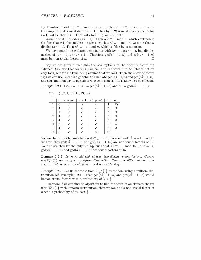
By definition of order ar ≡ 1 mod n, which implies ar − 1 ≡ 0 mod n. This inturn implies that n must divide ar − 1. Thus by (9.2) n must share some factor( 6= 1) with either (a

r2 − 1) or with (a

r2 + 1), or with both.

Assume that n divides (ar2 − 1). Then a

r2 ≡ 1 mod n, which contradicts

the fact that r is the smallest integer such that ar ≡ 1 mod n. Assume that ndivides (a

r2 + 1). Then a

r2 ≡ −1 mod n, which is false by assumption.

We have found the n shares some factor with (ar2 − 1)(a

r2 + 1), but divides

neither of (ar2 − 1) or (a

r2 + 1). Therefore gcd(a

r2 + 1, n) and gcd(a

r2 − 1, n)

must be non-trivial factors of n.

Say we are given a such that the assumptions in the above theorem aresatisfied. Say also that for this a we can find it’s order r in Z∗

n (this is not aneasy task, but for the time being assume that we can). Then the above theoremsays we can use Euclid’s algorithm to calculate gcd(a

r2 +1, n) and gcd(a

r2 −1, n),

and thus find non trivial factors of n. Euclid’s algorithm is known to be efficient.

Example 9.2.1. Let n = 15, d+ = gcd(ar2 + 1, 15) and d− = gcd(a

r2 − 1, 15).

Z∗15 = {1, 2, 4, 7, 8, 11, 13, 14}

a r r even? a 6= 1 ar2 6≡ −1 d+ d−

1 0 X × X 1 152 4 X X X 5 34 2 X X X 5 37 4 X X X 5 38 4 X X X 5 311 2 X X X 3 513 4 X X X 5 314 2 X X × 15 1

We see that for each case where a ∈ Z∗15, a 6= 1, r is even and a

r2 6≡ −1 mod 15

we have that gcd(ar2 + 1, 15) and gcd(a

r2 − 1, 15) are non-trivial factors of 15.

We also see that for the only a ∈ Z∗15 such that a

r2 ≡ −1 mod 15, i.e. a = 14,

gcd(ar2 + 1, 15) and gcd(a

r2 − 1, 15) are trivial factors of 15.

Lemma 9.2.2. Let n be odd with at least two distinct prime factors. Choosea ∈ Z∗

n\{1} randomly with uniform distribution. The probability that the orderr of a in Z∗

n is even and ar2 6≡ −1 mod n is at least 1

2 .

Example 9.2.2. Let us choose a from Z∗15\{1} at random using a uniform dis-

tribution (cf. Example 9.2.1). Then gcd(ar2 + 1, 15) and gcd(a

r2 − 1, 15) would

be non-trivial factors with a probability of 67 >

12 .

Therefore if we can find an algorithm to find the order of an element chosenfrom Z∗

n\{1} with uniform distribution, then we can find a non trivial factor ofn with a probability of at least 1

2 .


9.3 Shor’s Algorithm

For a given a ∈ Z∗n, its order r is the period of the function f : Z→ Zn

f(k) = ak mod n.

We will describe in this section an algorithm that uses the inverse QFT in Zn

to find the period of this function (with some probability), and then uses themethod from the previous section to find non trivial factors . We will give thealgorithm first, which if unfamiliar may seem to come out of the blue somewhat.We will then discuss the probability of it succeeding. Firstly we present a smalldiscussion about continued fractions.

Consider α ∈ Q>0. It should be clear that α has a finite continued fractionexpansion, i.e. there are α0, α1, . . . , αn ∈ N such that

α = α0 +1

α1 +1

α2 +1

.. . +1

αn

.

In such a case we write α = [α0, α1, . . . , αn]. The ith convergent of the continuedfraction expansion for α is defined to be

pi

qi= [α0, α1, . . . , αi].

Note that all the convergents can be found efficiently using Euclid’s algorithm(i.e. all the pi and qi). We will use the fact that the qi can be found efficientlyin the following algorithm, due to Shor [21].

The algorithm to find the order non trivial factors of n is as follows.

1. Pick a ∈ Zn\{1} randomly using a uniform distribution. A quantumcircuit as discussed in Chapter 8 could be used.

2. Calculate gcd(a, n) using Euclid’s algorithm. If gcd(a, n) > 0, this is anon-trivial factor of n and stop. Otherwise we know that a ∈ Z∗

n\{1}.3. Check if r < 19, simply by multiplying a together 19 times. If r < 19 then

skip to Step 11. This rather bizarre step is related to the probabilities ofthe algorithm succeeding and is explained more later.

4. Pick m such that m = 2i for some integer i and n2 ≤ m2 < 2n2.

5. Prepare two quantum registers in compound state |0〉 |0〉. Let one be largeenough to represent Zm Thus it must be of length (at least) i. Let theother be large enough to represent Zn - thus it must be of length at least jwhere 2j ≥ n. The register that represents Zm is written on the left, andthe register that represents Zn is written on the right. Thus for x ∈ Zm

and y ∈ Zn a typical pure state is written as |x〉 |y〉.6. Apply the Hadamard transform Hm. The resulting state is

1√m

m−1∑

k=0

|k〉 |0〉 .


7. Apply a map defined by |k〉 |0〉 7→ |k〉 |ak mod n〉. This results in state

1√m

m−1∑

k=0

|k〉 |ak〉 .

Note that the function k 7→ ak mod n had period r (which is unknown).Thus we can write the above superposition as

1√m

r−1∑

l=0

sl∑

q=0

|qr + l〉 |al〉 ,

where sl is the largest integer such that slr + l < m. We note that eachal < r. Thus roughly speaking in the above superposition, in the registeron the right, only the members of Zn that are less than the order r arepresent.

We also note that the left multiplier of each |al〉 is

sl∑

q=0

|qr + l〉 .

We can see that this superposition also contains information about r. Itis a superposition of basis states such that an |x〉 is in the superpositionif and only if x = qr + l for some q. This is essentially a sequence withperiod r. We use the inverse QFT to ‘extract’ this period.

8. Apply the inverse QFT in Zm to the register on the left. Thus the stateis

1√m

r−1∑

l=0

sl∑

q=0

1√m

m−1∑

p=0

e2πip(qr+l)

m |p〉 |al〉 . (9.3)

Don’t worry if this looks a bit unwieldy - the proof that shows this statewhen measured returns a ‘good’ result with high enough probability isomitted. We won’t directly use this state again.

9. Observe the register on the left. This results is some p ∈ Zm.

10. Apply Euclid’s algorithm to find the convergents pi

qiof p

m , and (try to)find the smallest qi such that aqi = 1 mod n. If such a qi is found thenqi is the order of a.

11. Use Euclid’s algorithm to calculate gcd(ar2 + 1, n) and gcd(a

r2 − 1, n). As

we will show, the probability that these are non trivial factors of n is atleast 1/20 log logn.

Remark 9.3.1. As already mentioned in Remark 9.1.1, Shor’s algorithm hasbeen implemented to factor 15 using a 7 qubit quantum computer. Using thenotation from the algorithm above, n = 15. We need to have a register capableof representing Zn, so we must have a register of length ⌈log2(15)⌉ = 4, i.e. 4qubits. We also need to have a register capable of representing Zm, where m ischosen such that n2 <= m < 2n2, and so the smallest such a register could beis ⌈log2(152)⌉ = 8 qubits. Thus we need at least 12 qubits. The method usedin [23] was some ‘cut down’ version of the algorithm.


We will now discuss the probability of this algorithm succeeding. The finalstep has already been discussed in the previous section. If we have managed tofind the order of the uniformly chosen element a, then the probability that thefinal step outputs non trivial factor(s) of n is at least 1

2 .However the previous steps do not guarantee that we can find this order.

We will now discuss how likely it is that we do. We need the following theorem,which we will not prove.

Theorem 9.3.1. If for a ∈ Q>0 and p, q ∈ N, gcd p, q = 1 and

0 <∣∣∣a− p

q

∣∣∣ ≤ 1

2q2

then pq is a convergent of the continued fraction expansion of a.

This theorem is easily applied to our situation.

Lemma 9.3.1. If for p, r, d,m, n ∈ N we have gcd(d, r) = 1, n2 ≤ m < 2n2,r < n and

∣∣∣p− dmr

∣∣∣ ≤ 1

2, (9.4)

then dr is a convergent of p

m .

Proof. Clearly we have

∣∣∣p

m− d

r

∣∣∣ =1

m

∣∣∣p− dmr

∣∣∣ ≤ 1

2m≤ 1

2n2

<1

2r2.

Therefore by Theorem 9.3.1 we have that dr is a convergent of p

m .

The above lemma shows that if we have measured (9.3) to find a p, such thatit is at most 1

2 away from some integer multiple, d, of mr , such that d satisfies

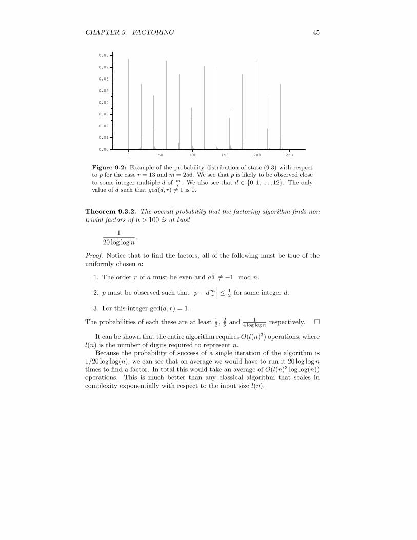
gcd(d, r) = 1, then step 10 will result in the correct order of a. A specific case isshown in Figure 9.2 that appears to show that it is likely that these requirementsare satisfied. We present the following lemmata for more general cases.

Lemma 9.3.2. For n > 100, observing (9.3) will result in p such that∣∣∣p−dm

r

∣∣∣ ≤12 for some integer d with a probability of at least 2

5 .

There is a one to one correspondence between p that satisfy (9.4), and d ∈{0, 1, . . . , r − 1}. Therefore observing p that satisfies equation (9.4) for some dessentially means that some d ∈ {0, 1, . . . , r − 1} is chosen (although we maynot know what it is). We would like to know, given a p that satisfies (9.4) forsome d, what the probability of that for this d satisfies gcd(d, r) = 1, which isthe additional requirement to invoke Lemma 9.3.1.

Lemma 9.3.3. For r > 19 and r < n the probability that a d chosen as abovesatisfies gcd(d, r) = 1 is as least 1/4 log logn

This previous lemma explains why the algorithm checks if the order of a isless than 19.


0 50 100 150 200 2500.00

0.01

0.02

0.03

0.04

0.05

0.06

0.07

0.08

Figure 9.2: Example of the probability distribution of state (9.3) with respectto p for the case r = 13 and m = 256. We see that p is likely to be observed closeto some integer multiple d of m

r. We also see that d ∈ {0, 1, . . . , 12}. The only

value of d such that gcd(d, r) 6= 1 is 0.

Theorem 9.3.2. The overall probability that the factoring algorithm finds nontrivial factors of n > 100 is at least

1

20 log logn.

Proof. Notice that to find the factors, all of the following must be true of theuniformly chosen a:

1. The order r of a must be even and ar2 6≡ −1 mod n.

2. p must be observed such that∣∣∣p− dm

r

∣∣∣ ≤ 12 for some integer d.

3. For this integer gcd(d, r) = 1.

The probabilities of each these are at least 12 , 2

5 and 14 log log n respectively.

It can be shown that the entire algorithm requires O(l(n)3) operations, wherel(n) is the number of digits required to represent n.

Because the probability of success of a single iteration of the algorithm is1/20 log log(n), we can see that on average we would have to run it 20 log logntimes to find a factor. In total this would take an average of O(l(n)3 log log(n))operations. This is much better than any classical algorithm that scales incomplexity exponentially with respect to the input size l(n).

Chapter 10

Searching

In this chapter we discuss a formalization of searching, show a few ways inwhich a quantum computer could (and couldn’t) search unsorted lists fasterthan conventional computer.

10.1 Blackbox Functions

Let us define a blackbox function as a function

f : Fm2 −→ F2

that returns its value instantly in one computational step, where the inner work-ings of f are unknown to us. We say our problem of searching some unsortedlist is equivalent to trying to find some x ∈ Fm

2 such that f(x) = 1. We callsuch x solutions to the searching problem.

We also define for some unknown y ∈ Fm2 , a blackbox function fy such that

fy(x) =

{1 if x = y

0 if x 6= y.

We say that searching in this case is trying to find y, when all we can do isquery f for some x. In this case there is only one solution, y.

Remark. Sometime a blackbox function is called an oracle, as it just ‘magically’outputs the result.

Example. We can order the elements of Fm2 . Notice that for x ∈ Fm

2 there arexi ∈ F2 such that x = (x0, x1, . . . , xm−1). This is a binary representation ofsome number in Z2m . Thus we have a natural order on Fm

2 , and we have alist. We can say that each place on the list, i.e. each element of Fm

2 , actuallyrepresents an entry of a phone book. A phone book is unsorted with respect tothe telephone numbers - if we are trying to find an entry with a given telephonenumber, we have no idea where in the phone book the listing may be. The onlyway is for us to check each line, see if the number given is equal to the one wewant. Our current place in the phone book which we are checking is x, the placein the phone book with the number we want is the unknown y, the phone bookitself is fy and the checking of each line is calling fy(x), which results in 1 ifthe line has the right number, and 0 if it hasn’t.

46

CHAPTER 10. SEARCHING 47

Remark. One may think that the idea of a blackbox function is a bit artificial ifwe are trying to relate this to some real world scenario - real world operationsare not instant. However it is a reasonable concept for working out probabilityof algorithms succeeding, and giving lower bounds on the number of operationsused.

If y is unknown, picking x1, x2, . . . , xk disjoint with uniform probability, andcalling f(xi) for each one would result in finding y with probability of k

2m .

Example. Consider again the phone book example, with the phone book con-taining n entries. Picking k entries in the phone book at random with uniformdistribution would find a solution with probability of k

n .

We can extend the idea of blackbox function to a quantum blackbox function.Given a traditional blackbox function f as above, define the quantum black boxfunction, or query operator, Qf to be the linear map such that

Qf |x〉 |b〉 = Qf |x〉 |b⊕ f(x)〉 ,

where x ∈ Fm2 , b ∈ F2, and ⊕ is addition modulo 2 (the group operation in

F2 = Z2). Thus |x〉 is the state of an m-length quantum register, known as theknown as the source register, and |b〉 is the state of a single qubit, the targetqubit. The map Qf is a permutation on an m + 1 dimensional Hilbert space,and so it is indeed unitary.

10.2 How Not To Search

We will describe in this section a perhaps naive way of using the query operatorQfy

that does not do any better than just guessing y. The steps are

1. Start with a source register of length m in state |0〉, and a single qubit,the target qubit in state |0〉. Thus the compound state is |0〉 |0〉.

2. Apply the Hadamard transform Hm to the source register. This results instate

1√2m

∑

x∈Fm2

|x〉 |0〉 .

3. Apply the query operator Qfyto result in state

1√2m

∑

x∈Fm2

|x〉 |fy(x)〉 .

4. Measure the register of length m.

Since the state of the register before measurement was just an equal weightingof all possible states |x〉, they probability that we find y using this method isthe same as if we just picked x at random with uniform distribution.


10.3 Single Query Without (Grover’s) Amplifi-cation

We improve the earlier method using Hadamard transforms. Firstly let us definethe modified query operator. Notice that the query operator Qf acting on state

|x〉 1√2(|0〉+ |1〉)

results in state

(−1)f(x) |x〉 1√2(|0〉+ |1〉).

Notice that in this case the application of the query operator has flipped theamplitude of |x〉 if and only if it is a solution to the searching problem, and hasleft the state of the target qubit as it was. We will no longer refer to the targetqubit, and treat it just as an ancilla qubit. The modified query operator is thusdefined to be the map

Vf |x〉 = (−1)f(x) |x〉 .

We will also require another map. Let f0 : Fm2 → F2 be defined to be

f0(x) =

{1 x = 0

0 otherwise.

By Chapter 4, this is can be constructed using a boolean circuit, and so it can beconstructed using some quantum circuit, using some ancilla qubits. The circuitwould perform the function

F0 |x〉 |0〉 = |x〉 |f0(x)〉 ,

where we omit writing the ancilla qubits. Note f0 is not a blackbox functionsince 0 is known.

We will also use the fact that the fourier transform in Fm2 is self inverse. This

means that the QFT in Fm2 is self inverse, i.e. the Hadamard transform Hm is

self inverse. Thus we can apply the map Hm to either side of the followingexpression to result in the other side

|y〉 Hm←−→ 1√2m

∑

x∈Fm2

(−1)x.y |x〉 , (10.1)

or to take the specific case of y = 0 we get

|0〉 Hm←−→ 1√2m

∑

x∈Fm2

|x〉 . (10.2)

Using these we are ready to describe a better algorithm for searching.

1. Start, as before, with a source register of length m in state |0〉.


2. Apply the Hadamard transform Hm to the source register. This results instate

1√2m

∑

x∈Fm2

|x〉 .

3. Apply the modified query operator Vfyto result in state

1√2m

∑

x∈Fm2

(−1)fy(x) |x〉 .

Remember that we are using an ancilla qubit that we are not writing.Notice also that this is an equal superposition of all states |x〉 wherex ∈ Fm

2 , but with the sign of state |y〉 inverted. If we were to measurethe system at this point, we would only find the solution y with the sameprobability as if we chose x at random using a uniform distribution.

4. Apply the Hadamard transform Hm to result in the map

1√2m

∑

x∈Fm2

(−1)fy(x) |x〉 =1√2m

((∑

x∈Fm2

|x〉)− 2 |y〉)

Hm7−−→ |0〉 − 2√2m

∑

x∈Fn2

(−1)x.y |x〉

=(1− 2√2m

) |0〉 − 2√2m

∑

x6=0

(−1)x.y |x〉

We use (10.1) and (10.2) to calculate the above.

5. We then apply F0 to the compound system of the register and an extraqubit (in state |0〉) to get

(1− 2√2m

) |0〉 |0〉 − 2√2m

∑

x6=0

(−1)x.y |x〉 |0〉

F07−−→(1− 2√2m

) |0〉 |1〉 − 2√2m

∑

x6=0

(−1)x.y |x〉 |0〉

Note that the resulting state is entangled.

6. Measure the extra qubit (the one on the right). From now on we ignorethis qubit (the state was entangled so the act of measurement has affectedthe source register).

State after measurement Probability|0〉 (1− 2

2m )21√

2m−1

∑x6=0(−1)x.y |x〉 1− (1− 2

2m )2

7. Apply the Hadamard transform Hm to the source register. Note that

∑

x6=0

(−1)x.y |x〉 =(∑

x∈Fn2

(−1)x.y |x〉)− |0〉 .


State after Hadamard transform Hm Probability1√2m

∑x∈Fm

2|x〉 (1− 2

2m )2

1√(2m−1)(2m)

((2m − 1) |y〉 −

∑x6=y |x〉

)1− (1− 2

2m )2

8. Measure the source register. If the state was that of the top row in theabove table, the probability that this measurement results in y is 1

2m . Ifthe state was that of the bottom row in the above table, the probability ofthat the measurement results in y is 2m−1

2m . Thus taking the probabilitiesof being in those states to start with into account, the overall probabilitythe this final measurement results in y is

1

2m(1− 2

2m)2 + (

2m − 1

2m)(1− (1− 2

2m)2)

=5

2m+

12

22m− 8

23m

≈ 5

2mfor large m.

This method makes a single query to the modified query operator. It returnsy with a probability of about 5

2m for large m. This is about 5 times betterthan making a single query by picking a single x randomly using a uniformdistribution.

10.4 Amplitude Amplification

In this section we describe a method of using unitary operators that, given asuperposition of uniform amplitudes

1√2

∑

x∈Fn2

|x〉 ,

will amplify the amplitude of those |x〉 such that f(x) = 1. Recall that aquantum state must be of unit length, so this amplification is only relative.Once the operator has amplified these amplitudes, observation is more likely tolead to a solution.

As earlier we will make use of the modified query operator Vf . We will alsoneed another map Rm such that

Rm |x〉 ={− |x〉 x = 0

|x〉 otherwise.

If we index 2m×2m matrices by Fm2 (taking the natural order defined by taking

the elements of Fm2 as binary representations of integers), we get that

Rm =

−1 0 0 . . . 00 1 0 . . . 00 0 1 . . . 0...

......

. . ....

0 0 0 . . . 1

.

We will omit how to decompose this map into a finite number of quantum gatesfor the sake of brevity.


Definition 10.4.1. Using the notation above, define Gm to be the unitary mapsuch that

Gm = −HmRmHmVf .

We say the map −HmRmHm is the inversion about average operator, for reasonsthat will become clear.

To get an idea of what HmRmHm does, we try to find what its matrix lookslike. We order the basis elements of Fm

2 by taking the elements of Fm2 to be a

binary representation of some integer. Firstly recall that

Hm =∑

x∈Fm2

(−1)x.y |x〉 .

Therefore (Hm)xy = 1√2m

(−1)x.y. Thus (we omit the working again for brevity)

(HmRmHm)xy = . . .

=

{− 2

2m x 6= y

1− 22m x = y

.

Therefore

HmRmHm =

1− 22m − 2

2m − 22m . . . − 2

2m

− 22m 1− 2

2m − 22m . . . − 2

2m

− 22m − 2

2m 1− 22m . . . − 2

2m

......

.... . .

...− 2

2m − 22m − 2

2m . . . 1− 22m

= I − 2P,

where P is the projection onto the subspace spanned by

|ψ〉 = 1√2

∑

x∈Fn2

|x〉 .

We would like to know the effect −HmRmHm has on a general state

∑

x∈Fn2

αx |x〉 .

We define the average of the amplitudes as

A =1√2

∑

x∈Fn2

αx,

and so we can see that∑

x∈Fn2

αx |x〉 = A∑

x∈Fn2

|x〉+∑

x∈Fn2

(αx −A) |x〉 .

The first term in the equation above is clearly part of the subspace spanned by|ψ〉. The second term is part of the orthogonal complement of that subspace,


as can be easily checked (by checking that the inner product of the two termsis equal to 0). Thus

−HmRmHm

∑

x∈Fn2

αx |x〉 = (2P − I)∑

x∈Fn2

αx |x〉

=∑

x∈Fn2

(2A− αx) |x〉 .

If some given |x〉 has amplitude αx ≈ A, then the map −HmRmHm wouldnot change the amplitude of |x〉 by very much. Conversely if some |x′〉 hasamplitude of αx′ ≈ −A, then the map −HmRmHm would approximately invertthis amplitude and multiply it by 3. This is why −HmRmHm is called inversionabout average.

10.4.1 Single Query, Single Solution

We can now describe Grover’s search algorithm [10] for the case when there isa single solution y.

1. Start with a quantum register of length m in state |0〉.

2. Apply the Hadamard transform Hm to get

1√2m

∑

x∈Fn2

|x〉 .

3. Apply the modified query operator Vfy. This results in state

1√2m

∑

x∈Fm2

(−1)fy(x) |x〉 .

Note that Vfyhas flipped the amplitude of |y〉 (although y is still un-

known).

4. Apply the map −HmRmHm. The average of the amplitudes (before ap-plying the map) was

A =1

2m

((2m − 1)

1√2m

+ (1)(−1√2m

)=

1√2m

(1− 2

2m

).

Thus −HmRmHm performs the map

1√2m

∑

x∈Fm2

(−1)fy(x) |x〉 =1√2m

∑

x6=y

|x〉+ (− 1√2m

) |y〉

−HmRmHm7−−−−−−−−→(2A− 1√2m

)∑

x6=y

|x〉+ (2A+1√2m

) |y〉

=1√2m

(1− 4

2m

)∑

x6=y

|x〉+ 1√2m

(3− 4

2m

)|y〉 .


5. Measure the system. This results in y with probability 12m (3− 4

2m )2 ≈ 92m

for large m. This is approximately 9 times better than choosing any x atrandom using a uniform distribution.

Remark 10.4.1. Grover’s search algorithm has been carried out on a two qubitNMR computer [12].

10.4.2 Known Number of Solutions

Let us now assume that a blackbox function f : F2m → F2 has k solutions. Let T

be the set of solutions and F be the rest of F2m. Thus |T | = k. From the previous

section we can see that given a uniform superposition of all the representativesof F2

m,

1√2m

∑

x∈Fm2

|x〉 , (10.3)

the operator Gm keeps the amplitudes of |x〉 such that x ∈ T all the same,and it keeps all the amplitudes of |x〉 such that x ∈ F the same. Thus after rapplications of Gm to (10.3) we know that the state of the system is

tr∑

x∈T

|x〉+ fr

∑

x∈F

|x〉 , (10.4)

for some tr, fr ∈ C dependant on r. Our aim is to try to find r such that tris maximised. To do this we can, and will, find tr and fr explicitly in terms ofk and m. To achieve that, we will create a recurrence relation, i.e. find tr+1

and fr+1 in terms of tr and fr, and then solve it using the initial conditionst0 = f0 = 1√

2m.

Lemma 10.4.1. Let all notation be as above.(tr+1

fr+1

)=

(1− 2k

2m 2− 2k2m

− 2k2m 1− 2k

2m

)(trfr

)(10.5)

Proof. Apply the modified query operator Vf to (10.4) to result in

−tr∑

x∈T

|x〉+ fr

∑

x∈F

|x〉 .

The average of the amplitudes in the above expression is

A =1

2m

(−trk + fr(2

m − k)).

Application of the operator −HmRmHm results in

(2A+ tr)∑

x∈T

|x〉+ (2A− fr)∑

x∈F

|x〉 .

We have now applied Gm r + 1 times, so in fact tr+1 = 2A + tr, and fr+1 =2A− tr. Expanding out these expressions gives us the result.


Lemma 10.4.2. Let all notation be as above. Then the solution to (10.5) withthe initial conditions t0 = f0 = 1√

2mis

tr =1√k

sin((2r + 1)θ0

)

fr =1√

2m − kcos((2r + 1)θ0

),

where θ0 ∈ [0, π2 ] is chosen such that sin2 θ0 = k

2m .

Proof. This is an exercise in recurrence relations and so will be omitted. See [11]for a proof.

Lemma 10.4.3. The probability of seeing a solution after r applications of Gm

is sin2((2r + 1)θ0).

Proof. After r iterations the state of the system is

tr∑

x∈T

|x〉+ fr

∑

x∈F

|x〉 . (10.6)

Thus the probability of observing any solution, i.e. any x ∈ T , is equal to |T |t2r =kt2r. By Lemma 10.4.2 we have that this must be equal to sin2((2r + 1)θ0)

This leads to a surprising, albeit not always that useful, result.

Lemma 10.4.4. Let k = 14 .2

m. Applying Gm once and then measuring thesystem would result in a solution with certainty.

Proof. If k = 14 .2

m then sin2 θ0 = 14 which implies θ0 = π

6 . Then by 10.4.3 the

probability of finding a solution after one application of Gm is sin2(π2 ) = 1.

However there are clearly cases when k 6= 14 .2

m.

Theorem 10.4.1. Let f : F2m → F2 be a blackbox function with k unknown

solutions in F2m. Assume that 0 < k ≤ 3

4 .2m. Let θ0 ∈ [0, π

3 ) be such that

sin2 θ0 = k2m . Then applying Gm exactly ⌊ π

4θ0⌋ times to (10.3) and then mea-

suring the system would result in a solution with a probability of at least 14 .

Proof. By Lemma 10.4.3 the probability of seeing a solution after ⌊ π4θ0⌋ it-

erations is sin2((2⌊ π4θ0⌋ + 1)θ0). Thus we try to give a lower bound for this

probability. For some |δ| ≤ 12

⌊π

4θ0

⌋= −1

2+

π

4θ0+ δ,

so(

2

⌊π

4θ0

⌋+ 1

)θ0 =

π

2+ 2δθ0.

Therefore∣∣∣∣(

2

⌊π

4θ0

⌋+ 1

)θ0 −

π

2

∣∣∣∣ = |2δθ0| ≤π

3.


Since the (absolute value of the) derivative of sin2 is always less than or equalto 1, we must have that

sin2((2

⌊π

4θ0

⌋+ 1)θ0) ≥ sin2(

π

2− π

3) =

1

4.

Now it should be more or less clear what the algorithm is. Remember k, thenumber of solutions, is known.

1. If k > 34 .2

m, pick x at random with uniform probability (perhaps usingthe random number generator from Chapter 8), and stop. In this case theprobability of x being a solution is clearly at least 3

4 .

2. Otherwise start with a quantum register of length m in state |0〉.

3. Apply the Hadamard transform Hm to get a uniform superposition of allthe basis states

1√2m

∑

x∈Fm2

|x〉 .

4. Apply the operator Gm exactly ⌊ π4θ0⌋ times.

5. Measure the system. By Theorem 10.4.1 the probability of finding a so-lution is at least 1

4 .

We can easily compare to the classical case when k = 1 and n is large.Roughly speaking, for small θ, sin θ ≈ θ. Thus for large n, 1

2m is small, so

θ0 ≈ 1√2m

, which in turn implies ⌊ π4θ0⌋ ≈ π

4

√2m. Thus the above algorithm

performs O(√

2m) queries to find a solution with a probability of 14 . A search

picking x at random with uniform probability would have to make 142m = O(2m)

queries to find a solution with probability of 14 .

10.4.3 Unknown Number of Solutions

Often we may not know how many solutions there are previous to a search,i.e. k is unknown. The algorithm in the previous section chose the number ofthe of times to apply Gm using k. The following theorem, which we will notprove, gives us a way to pick a number of times to apply Gm without previousknowledge of k.

Theorem 10.4.2. Let f : F2m → F2 be a blackbox function with k solutions in

F2m. Assume that 0 < k ≤ 3

4 .2m. Let d be an integer such that d ≥

√2m. Let r

be a uniformly chosen r ∈ {0, 1, . . . , d− 1}. Then applying Gm exactly r timesto (10.3) would result in a solution with probability of at least 1

4 .

Thus we present the following modified version of Grover’s algorithm, whichis in fact a simplified version of [6]. Remember that the number of solutions kis unknown.

1. Pick an x ∈ Fm2 randomly with uniform distribution. If f(x) = 1, then

stop.


2. Let d =⌊√

2m⌋

+ 1.

3. Choose an integer r ∈ {0, 1, . . . , d−1} randomly with uniform distribution,perhaps using the quantum circuit describe in Chapter 8.

4. Apply the Hadamard transform Hm on a quantum register of length at min state |0〉 to get a uniform superposition of all the basis states

1√2m

∑

x∈Fm2

|x〉 .

5. Apply the operator Gm exactly r times.

6. Measure the system.

We know that there must be k solutions to the searching problem, it’s just thatwe don’t know the value of k. If k > 3

4 .2m, then step 1 has output a solution

with a probability of at least 34 . If k ≤ 3

4 .2m, then Theorem 10.4.2 tells us that

the probability of getting a solution from step 6 is at least 14 . In either case,

the probability of getting a solution is at least 14 , performing (at most) O(

√2m)

queries. Thus finding a solution would, on average, require the algorithm to berun 4 times, which would still take O(

√2m) queries. A classical algorithm that

would on average require O(2m) queries.

Chapter 11

Conclusion

We have merely skimmed the surface of what is theoretically possible usingthe effects of superposition of states as described in Chapter 2. By the resultsin Chapter 4 we have shown the unitary operations, which are the allowableoperations on states, can be put together to make a circuit that will performthe same task as any classical boolean circuit. There would only be little pointif a quantum computer could only perform those operations.

Note we say little point and not no point. We haven’t yet mentioned it, butthe speed of current classical processors, essentially very complicated booleancircuits, is limited largely by the fact that each operation produces heat, whichis difficult to disperse. If current processors get too hot they essentially meltand become useless. As discussed in Chapter 3, operations in a quantum circuitare unitary maps, and are thus invertible. We will not get into the physics toexplain why, but this means that quantum operations would produce no heat,and so the speed of a quantum circuit should not be limited by heat production.

Also we have shown that there is a way to send two classical bits using onequantum bit in Chapter 5. We have shown that it is possible to teleport the stateof a quantum bit, but not to copy a general state in Chapter 6. Both of theseprotocols use entangled particles, as described in Chapter 2, these are particlesthat are somehow linked together, where the measurement of one affects theother.

Chapter 10 showed methods by which quantum circuits could be used tosearch large unsorted databases taking fewer queries than a classical computer,and said that a very simple case had been carried out (cf. Remark 10.4.1).

In Chapter 9 we have described Shor’s algorithm, part of which can be runon a classical computer, and part of which must be run on a quantum com-puter, that factors integers in polynomial time. As explained in Remarks 9.1.1and 9.3.1, this has only been carried out using a 7 qubit NMR quantum com-puter. However, it is difficult to scale up NMR computers to have enough qubitsto factor large numbers. We quote Shor himself,

“If you’re going to factor a 200-digit number, you’re going to needthousands of qubits. The road from 7 to thousands is a long one.”

Factoring large integers could theoretically crack current encryption schemessuch as RSA. This leads to the rather obvious question of whether, if quantumcomputers will be able to factor large integers, is it possible to have some sort of

57

CHAPTER 11. CONCLUSION 58

encryption schemes that are not crackable by quantum computers? The answerto this question is yes. There are encryption schemes, some of which are alreadyavailable commercially, that use quantum properties to encrypt and send data.These use similar methods to the quantum teleportation protocol in Chapter 6.Schemes that detect if someone is eavesdropping on a transmission are alsoknown.

Another field of quantum algorithms, that has not been mentioned, is thefield of quantum error correction algorithms. These are schemes that cor-rect some errors introduced during computation due to decoherence (cf. Re-mark 2.0.2). However, if the level of error is too high, which at the moment itis, these schemes offer little help.

In summary quantum computers have theoretically great potential, howeverdecoherence is a problem that is still a long way from being solved.

Bibliography

[1] A. Barenco, C. H. Bennett, R. Cleve, D. P. DiVincenzo, N. Margolus,P. Shor, T. Sleator, J. Smolin and H. Weinfurter: Elementary gates forquantum computation, Physical Review A 52:5, 3457-3467 (1995).

[2] J.S. Bell: On the Einstein Podolsky Rosen paradox, Physics 1:3, 195-200(1964).

[3] Charles H. Bennett, Gilles Brassard, Claude Crepeau, Richard Jozsa, AsherPeres, and William K. Wootters: Teleporting an unknown quantum statevia dual classical and Einstein-Podolsky-Rosen channels, Physical ReviewLetters 70, 1895-1899 (1993).

[4] Charles H. Bennet and Stephen J. Wiesner: Communication via one- andtwo-particle operators on Einstein-Podolsky-Rosen states, Physical ReviewLetters 69:20, 2881-2884 (1992).

[5] G.P. Berman, G.D. Doolen, R. Mainieri and V. I. Tsifrinovich: Introductionto quantum computers, Word Scientific, (1998).

[6] Michel Boyer, Gilles Brassard, Peter Hoeyer, Alain Tapp: Tight bounds onquantum searching, Fourth Workshop on Physics and Computation, 36-43(1996).

[7] W. Clearwater: Ultimate zero and one, Copernicus (2000).

[8] A. Einstein, B. Podolsky and N. Rosen: Can quantum-mechanical descrip-tion of physical reality be considered complete? Physical Review 41, 777-780(1935).

[9] Oded Goldreich: Foundations of cryptography: basic tools, Cambridge Uni-versity Press (2001).

[10] L. K. Grover: A fast quantum mechanical algorithm for database search,Proceedings of 28th Annual ACM Symposium on the Theory of Computing,212-219 (1996).

[11] Mika Hirvensalo: Quantum Computing: Second Edition, Springer (2003).

[12] J. A. Jones, M. Mosca and R. H. Hansen: Implementation of a quantumsearch algorithm on a nuclear magnetic resonance quantum computer, Na-ture 393, 344-346 (1998).

59

BIBLIOGRAPHY 60

[13] Laszlo B. Kish: End of Moores law: thermal (noise) death of integration inmicro and nano electronics, Physics Letters A 305, 144149 (2002).

[14] C. Lavor, L. R. U. Manssur and R. Portugal: Shor’s algorithm for factoringlarge integers, Laboratorio Nacional de Computacao Cientıfica (2004).

[15] I. Marcikic, H. de Riedmatten, W. Tittel, H. Zbinden, M. Legre, and N.Gisin: Distribution of time-bin entangled qubits over 50 km of optical fiber,Physical Review Letters 93:18, 1805021-1805024 (2004).

[16] M. Nielsen and I. Chuang: Quantum computation and quantum informa-tion, Cambridge University Press (2000).

[17] J. L. O’Brien, G. J. Pryde, A. G. White, T. C. Ralph amd D. Branning:Demonstration of an all-optical quantum controlled-NOT gate Nature 426,264-267 (2003).

[18] Emil Post: The two-valued iterative systems of mathematical logic, Annalsof Mathematics Studies, Princeton University Press (1941).

[19] K. J. Resch, M. Lindenthal, B. Blauensteiner, H. R. Bhm, A. Fedrizzi, C.Kurtsiefer, A. Poppe, T. Schmitt-Manderbach, M. Taraba, R. Ursin, P.Walther, H. Weier, H. Weinfurter, and A. Zeilinger: Distributing entangle-ment and single photons through an intra-city, free-space quantum channel,Optics Express 13, 202-209 (2005).

[20] Yaoyun Shi: Both Toffoli and controlled-NOT need little help to do univer-sal quantum computation, Quantum Information and Computation, 3:1,84-92 (2003).

[21] Peter W. Shor: Algorithms for quantum computation: discrete logarithmsand factoring, Proceedings of the 35th annual symposium on foundationsof computer science, 124134 (1994).

[22] Rupert Ursin, Thomas Jennewein, Markus Aspelmeyer, Rainer Kaltenbaek,Michael Lindenthal, Philip Walther and Anton Zeilinger: Communications:Quantum teleportation across the Danube Nature 430, 849-849 (2004).

[23] M. K. Vandersypen, M. Steffen, G. Breyta, C. S. Yannoni, M. Sherwood,and I. L. Chuang: Experimental realization of Shor’s quantum factoringalgorithm using nuclear magnetic resonance, Nature 414, 883-887 (2001).

[24] John Waltrous: Introduction to quantum computation: lecture notes, Uni-versity of Calgary (2005).

[25] W. K. Wootters and W. H. Zurek: A single quantum cannot be clonedNature 299, 802-803 (1982).

[26] T. Yamamoto, Yu. A. Pashkin, O. Astafiev, Y. Nakamura and J. S. Tsai:Demonstration of conditional gate operation using superconducting chargequbits, Nature 425, 941-944 (2003).

an introduction quantum computing - · pdf fileacknowledgments special thanks are given to...

Documents