an interior penalty method for optimal control problems with...

OPTIMAL CONTROL APPLICATIONS AND METHODSOptim. Control Appl. Meth. (2014)Published online in Wiley Online Library (wileyonlinelibrary.com). DOI: 10.1002/oca.2134

An interior penalty method for optimal control problems with stateand input constraints of nonlinear systems

P. Malisani1, F. Chaplais2 and N. Petit2,*,†

1EDF R&D Centre des Renardières Route de Sens 77818 Moret-sur-Loing, France2MINES ParisTech, PSL Research University, CAS - Centre automatique et systèmes,

60 bd St Michel 75006 Paris, France

SUMMARY

This paper exposes a methodology to solve state and input constrained optimal control problems for nonlin-ear systems. In the presented ‘interior penalty’ approach, constraints are penalized in a way that guaranteesthe strict interiority of the approaching solutions. This property allows one to invoke simple (without con-straints) stationarity conditions to characterize the unknowns. A constructive choice for the penalty functionsis exhibited. The property of interiority is established, and practical guidelines for implementation aregiven. A numerical benchmark example is given for illustration. © 2014 The Authors. Optimal ControlApplications and Methods published by John Wiley & Sons, Ltd.

Received 22 May 2013; Revised 25 November 2013; Accepted 25 June 2014

KEY WORDS: optimal control; constraints; state constraints; interior methods; penalty design

1. INTRODUCTION

This paper exposes a methodology allowing one to solve constrained optimal control problems(COCP) for general multi-input multi-output system with nonlinear dynamics. This methodologybelongs to the class of interior point methods (IPMs), commonly considered in finite-dimensionaloptimization, which consists in approaching the optimum by a path strictly lying inside the con-straints. A main motivation for using this approach is that, in the interior, optimality conditions aremuch easier to formulate explicitly.

The idea driving penalty methods (for both finite-dimensional optimization problems and optimalcontrol problems) is as follows. An augmented performance index is considered. It is constructedas the sum of the original cost function and so-called penalty functions that have some divergingasymptotic behavior when the constraints are approached by any tentative solution. This augmentedperformance index can then be optimized in the absence of constraints, yielding a biased estimateof the solution of the original problem. Two kinds of penalty methods exist: exterior penalty andinterior penalty (a.k.a. barrier methods). In both approaches, minimization of the augmented per-formance index favors satisfaction of the constraints, depending on the weight of the penalty. Inexterior penalty methods, for each augmented problem, the solution usually violates the constraints.The weight factor of the penalty should be increased so that this violation becomes sufficientlysmall. When this parameter is varied, the successive solutions generate a path lying outside of the

*Correspondence to: N. Petit, MINES ParisTech, PSL Research University, CAS - Centre automatique et systèmes,60 bd St Michel 75006 Paris, France.

†E-mail: [email protected] is an open access article under the terms of the Creative Commons Attribution License, which permits use,distribution and reproduction in any medium, provided the original work is properly cited.

© 2014 The Authors. Optimal Control Applications and Methods published by John Wiley & Sons, Ltd.

http://creativecommons.org/licenses/by/3.0/

P. MALISANI, F. CHAPLAIS AND N. PETIT

constraints. In IPMs, by construction, only feasible solutions are generated, but these are biased(suboptimal). The weight factor should be set sufficiently small to reduce the bias to an accept-able value. From a practical viewpoint, exterior methods are usually considered as more robust thaninterior ones. On the other hand, interior methods are attractive because they generate only feasi-ble solutions. This can be an interesting particularity in numerous applications of automatic control(especially in closed-loop receding horizon approaches where satisfaction of constraints is moreimportant than optimality; see [1] and references therein). All penalty methods are computationallyappealing, as they yield unconstrained problems for which a vast range of highly effective algo-rithms are available. In finite-dimensional optimization, outstanding algorithms have resulted fromthe careful analysis of the choice of penalty functions and the sequence of weights. In particular, theIPMs that are nowadays implemented in successful software packages such as KNITRO [2], OOQP[3] have their foundations in these approaches. We refer the interested reader to [4] for a historicalperspective on this topic.

In this article, we apply similar penalty methods to solve COCPs in a spirit similar to [5–8].COCPs represent a very handy formulation of objectives in numerous applications, especiallybecause constraints are very natural in problems of engineering interest. Unfortunately, these con-straints induce some serious difficulties [9–11]. In particular, it is a well-known fact (see, e.g., [11])that constraints bearing on state variables are difficult to characterize, as they generate both con-strained and unconstrained arcs along the optimal trajectory. To determine optimality conditions, itis usually necessary to know or to a priori postulate the sequence and the nature of the arcs con-stituting the desired optimal trajectory. Active or inactive parts of the trajectory split the optimalitysystem in as many coupled subsets of algebraic and differential equations. Yet, not much is knownon this sequence, and this often results in a high complexity. Therefore, it is often preferred to usea discretization-based approach to this problem, and to treat it, for example, through a collocationmethod [12], as a finite-dimensional problem [13–19]. Under this finite-dimensional form, IPMshave been applied to optimal control problems in [20–22] and [23]. This is not the path that weexplore, as we want to deal with optimal control problems under their original infinite-dimensionalrepresentation.

There is a well-established literature on the mathematical foundations of IPMs for finite-dimensional mathematical programming [3]. There exist also recent works in the field of exactpenalty methods for various types of optimal control problem [24–29]. These methods are of par-ticular interest because each solution of the sequence of optimal control problem is easily computedusing classical stationarity conditions of the solution. The problem can be formulated, for example,by parameterizing the control variables using a finite number of values and switching times (to bedetermined). The constraints, on the state and control variables, and the dynamics can be expressedin terms of the unknowns and eventually treated as penalties. After the sensitivities of the objec-tive function with respect to these unknowns are computed, iterative descent algorithms can be usedto generate the solution. Nonsmooth methods can also be employed, depending on the smoothnessof the constraints transcription [29]. In IPMs, the main difficulty is to guarantee that the sequenceof solution is strictly interior. This point is critical because interiority is a requirement to avoidill-posedness and computational failure of implemented algorithms. The problem of interiority ininfinite-dimensional optimization has been addressed in [30] for input-constrained optimal control,and in [31–33], respectively, for linear systems, single input single output nonlinear systems, andmulti-variable nonlinear systems with cubic input constraints. These contributions provide penaltyfunctions guaranteeing the interiority of the solutions. The purpose of this article is to propose asynthetic view by generalizing previous historic and more recent results to nonlinear systems whoseinputs belong to a general convex set, using new elements of proof and to expose the method in afriendly way for practitioners.

The paper is organized as follows. Section 2 contains the problem statement and sketches thecontribution. Sections 3–5 present progressively eliminate the constraints from the formulation ofthe penalized problems. In Section 3, it is shown that a suitable choice of the state penalty guar-antees that any trajectory yielding a finite cost is interior. In Section 4, a control penalty is added.Together with the state penalty, they guarantee that any optimal control for the penalized problemlies in the interior of the control constraints with a state that is in the interior of the state constraints.

© 2014 The Authors. Optimal Control Applications and Methodspublished by John Wiley & Sons, Ltd.

Optim. Control Appl. Meth. (2014)DOI: 10.1002/oca

INTERIOR METHOD IN CONSTRAINED OPTIMAL CONTROL

Capitalizing on the interiority of the previous optimal controls, Section 5 uses a so-called satura-tion functions to transform the control constrained problem of Section 4 into a fully unconstrainedoptimal control problem. Section 6 recalls the convergence of the costs, and a classic convexity argu-ment shows the convergence of the optimal controls and states for the penalized problems. Solvingalgorithms are presented in Section 7. For convenience, a practical guide or ‘cookbook’ is proposedto help the users in deriving the equations needed for implementation. Section 8 gives a numeri-cal application of the previous methods and algorithms by solving the Goddard problem [34] withan atmospheric pressure constraint. The source code for this example is freely available for inter-ested readers. Finally, Section 9 gives conclusions and perspectives. It is followed by appendicescontaining several proofs that have been omitted from the main stream of the paper, and a recall (inAppendix A) of the general convergence result by Fiacco and McCormick, which is inspirational tothe presented work.

2. NOTATIONS, PROBLEM STATEMENT, AND PRESENTATION OF THE CONTRIBUTION

The COCP that we wish to determine a solution method for in this article is to determine u� a globalsolution of

minu2U\X

"J.u/ D

Z T

0

`.xu; u/dt

#(1)

for the dynamics

Pxu.t/ D f .xu.t/; u.t//; x.0/ D x0 (2)

where ` W Rn�Rm 7! R is a locally Lipschitz function of its arguments, continuously differentiablewith respect to u, xu.t/ 2 Rn and u.t/ 2 Rm are the state and the control, which satisfy the(multi-input multi-output) nonlinear dynamics (2), f is continuously differentiable, for someD > 0kf .x; u/k 6 D.1Ckxk/; 8x 2 Rn;8u 2 C, where C is a bounded closed subset of Rm defined by

C ,°u D .u1; : : : ; up/ 2 Rm1 � : : : �Rmp ; p > 1; with

Xmi D m s.t. ui 2 Ci � Rmi

±where each Ci is a bounded closed convex subset of Rmi , which has a nonempty interior containing0 with continuously differentiable boundary.‡

The set U \ X is defined by control and state constraints that we detail below. The controlu W R 7! Rm is constrained to belong to the following set, which is closed and convex§

U , ¹u 2 L1.Œ0; T �;Rm/ s.t. u.t/ 2 C a.e. t 2 Œ0; T �º (3)

The set X is defined as follows

X ,®u 2 L1.Œ0; T �;Rm/ s.t. xu.t/ 2 X ad for all t 2 Œ0; T �

¯(4)

where

Xad , ¹x 2 Rn s.t. gi .x/ 6 0; i D 1; : : : ; qº

where the gi are continuously differentiable functions ¶ Rn7! R.

To implement IPMs, we shall naturally make the following assumption.

‡For example, this setting allows one to consider the case where C is ¹u 2 R3 s.t. u21C u2

26 1 ; ju3j 6 1º. The

boundary of C is not differentiable, yet u 2 C can be rewritten as u D .u1; u2/, where u1 belongs to an appropriateEuclidean disk and u2 belongs to an appropriate segment of R. Conveniently, the employed formalism covers the casewhere C is a hypercube.

§A proof of this statement is given in Appendix B.¶Observe thatXad is convex if the functions gi are convex.




Assumption 1 (strict interiority of the initial condition)The initial condition x0 of (2) belongs to the open set||

ı

X ad, ¹x 2 Rn s.t. gi .x/ < 0; i D 1; : : : ; qº

2.1. Summary of the contribution

The contribution of this article is an interior penalty method, which uses a so-called penalty functionsp1 and p2 and a so-called generalized saturation function � to formulate the following problem

min�2L1.Œ0;T �;Rm/

Z T

0

`�x�.�/; �.�/

�dt C �

Z T

0

p1

�x�.�/

�C p2.�/dt (5)

which is shown to generate, as � ! 0 a sequence of solutions converging to a solution of theCOCP defined earlier. Each solution in the sequence is relatively easy to determine as the prob-lem (5) is unconstrained. The next sections explain how p1, p2, and � are constructed and establishequivalence and convergence results. A tutorial summary is given in the ‘cookbook’ of Section 7.1.

3. ELIMINATION OF THE STATE CONSTRAINT BY STATE PENALTY

A first step of the methodology we propose is to penalize the state constraints.

3.1. State penalty

We introduce a state penalty function �g W .�1;C1/ ! Œ0;C1/, which satisfies the followingassumption.

Assumption 2 (Properties of the state penalty)The function �g is positive, continuously differentiable, convex, and increasing over ¹x < 0º. It isnull over ¹x > 0º. It is singular in 0� as limx"0 �g.x/ D C1.

To address the state constraints defined in (4), the following integral state penalty is introduced,for u 2 U

Pg.u/ D

Z T

0

qXiD1

�g ı gi.xu/dt

where ı denotes the function composition. To study the impact of this penalty, we introduce thenotations

X strict D

²u 2 L1.Œ0; T �;Rm/ s.t. xu.t/ 2

ı

X ad 8t 2 Œ0; T �

³U n X strict D

®u 2 U s.t. u … X strict

¯As will appear, one can determine a sufficient condition on the state penalty �g ensuring that anycontrol u 2 U yielding a bounded penalty Pg.u/ necessarily belongs to X strict.

Definition 1 (Proximity to a constraint)For any constraint gi , we define the proximity to the constraint as

˛ 7! �gi .u; ˛/ D meas .¹t 2 Œ0; T � s.t. 0 > gi .xu.t// > �˛º/ (6)

where meas.:/ is the Lebesgue measure of its argument.

||The setı

Xad is an open set. Moreover, if Assumption 1 holds and if the functions gi are convex, thenı

Xad is dense inXad. A proof of this result can be found in Appendix C.




Proposition 1 (Unboundedness of integral penalty)If, for all u 2 U n X strict, the penalty function �g satisfies

lim˛#0

�g.�˛/�gi .u; ˛/ D C1 (7)

then 8u 2 U n X strict

Pg.u/ D C1

ProofLet u 2 UnX strict, then there exists an index i such that maxt2Œ0;T � gi .x.t// > 0. Because �g.x/ D 0when x > 0, we have

Ii,Z T

0

�g.gi .x.t///dt D

Z0>gi .x.t//

�g.gi .x.t///dt

Moreover, because �g > 0, we have, for ˛ > 0,

Ii >Z0>gi .x.t//>�˛

�g.gi .x.t///dt , Ji .˛/

The state penalty satisfies �g > 0 on .�1; 0/; thus, Ji .˛/ is a nondecreasing positive continuousfunction of ˛ > 0, which satisfies

inf˛>0

Ji .˛/ D lim˛#0

Ji .˛/ , Ji .0C/

Because �g is increasing and because the Lebesgue measure is right-continuous (see, e.g., [35])

J .0C/ D lim˛#0

Z0>gi .x.t//>�˛

�g.gi .x.t///dt

> lim˛#0

Z0>gi .x.t//>�˛

�g.�˛/dt D lim˛#0

�g.�˛/�gi .u; ˛/

with �gi .u; ˛/ the Lebesgue measure defined in (6). If (7) holds, then Ji .0C/ D C1, whichimplies that Ii D C1. As a consequence, Pg.u/ D C1. This concludes the proof. �

Because the measure �gi .u; ˛/, which appears in (7), involves the control u, it is handy to give alower bound of it when u spans U n X strict.

Proposition 2 (Lower-bound on the proximity to a constraint)Under Assumption 1, ˛0 , �maxi .gi .x0// > 0. Then, there exists a constant � < C1 such thatfor all ˛ 2 Œ0; ˛0�, for all u 2 U n X strict the measure �gi .u; ˛/ defined in (6) is lower-bounded asfollows

�gi .u; ˛/ >˛

�

The proof is given in Appendix D.

3.2. First main result

Collecting Propositions 1 and 2, one finally obtains our first main result.

Theorem 1 (Interiority of the state)Under Assumptions 1 and 2, if the state penalty �g is such that

lim˛#0

˛�g.�˛/ D C1 (8)

then for every control u 2 U , the penalty value Pg.u/ is finite if and only if u 2 X strict.




To satisfy (8), a possible choice for �g is

�g.x/ D

².�x/�ng ; ng > 1; for x < 00 otherwise

(9)

ProofIf (8) holds, then we derive from Proposition 2 that (7) holds for u 2 U nX strict. From Proposition 1,we derive that Pg.u/ < C1 for u 2 U only if u 2 U \X strict. Conversely, if 2 U \X strict, then thetrajectories are well defined and continuous; therefore, the maximum value of gi .t/ for t 2 Œ0; T �and any i is strictly negative and the penalty Pg.u/ is finite because �u is bounded. Finally, oneeasily verifies that the penalty function defined by (9) satisfies Assumption 2 and (8). �

3.3. Introduction of a first penalized problem

Corollary 1Under the assumptions of Theorem 1, for every � > 0, the three following problems are equivalent

minu2U

J.u/C �Pg.u/ (10)

minu2U\X

J.u/C �Pg.u/ (11)

minu2U\X strict

J.u/C �Pg.u/ (12)

in the sense that they have the same set of minimizers and the same optimal values. In addition, thepenalty Pg in problem (12) is bounded for all of the controls in the given control set.

ProofObviously, the values of each minimum are in increasing order. However, to be optimal for prob-lems (10) and (11), a control u must belong to U and to X strict. Therefore, the optimum for (12) issmaller or equal to the optimum for (10), and they are all equal, and their minimizers all belong toU \ X strict. Finally, (12) yields a finite penalty by application of Theorem 1. �

Furthering Corollary 1, we now wish to let � ! 0 in (10), or equivalently (11) or (12). However,this requires to have a minimizing sequence for which the penalty is bounded, that is, that belongsto U \ X strict. Therefore, we make the following assumption.

Assumption 3 (Existence of an approaching interior sequence)Let v0 D infu2U\X J.u/. For any ! > 0, there exists s.!/ 2 U \ X strict such that v0 6 J.s.!// 6v0 C !.

This assumption is satisfied if, for instance, U\X strict is dense in U\X for the sup norm, becauseJ is continuous (Proposition 13).

Proposition 3Assume that the gi are convex, that the dynamics (2) is linear, and that U \ X strict is not empty.Then, X and X strict are convex, and U \X strict is dense in U \X for the sup norm, and consequently,Assumption 3 is satisfied.

ProofWith linear dynamics, for 2 Œ0; 1�, and two controls u and v, x�uC.1��/v D xu C .1 � /xv .Because the gi are convex, we have

gi

�x�uC.1��/v.t/

�D gi.x

u.t/C .1 � /xv.t// 6 gi .xu.t//C .1 � /gi .xv.t//




If we take u; v 2 X , this proves that X is convex. Similarly, if u; v 2 X strict, this proves that X strict

is convex. Finally, by taking u 2 U \X strict (which is nonempty) and v 2 U \X and 2 .0; 1/, weobtain

gi

�x�uC.1��/v.t/

�6 gi .xu.t// < 0

Also, uC .1 � /v 2 U because U is convex and closed. By letting tend to 0, this proves thatU \ X strict is dense in U \ X for the sup norm. �

Corollary 2Assume also that for � small enough, Penalized Optimal Control Problem (POCP) (10) has at leasta minimizer u�.�/, and that Assumption 3 holds. Then,

A lim�#0 J.u�.�// D infu2U\X J.u/

B lim�#0 �Pg.u�.�// D 0

ProofBecause of Corollary 1, u�.�/ is also a solution of (11) and (12), and we can apply theclassic Theorem 5 by Fiacco and McCormick, recalled for convenience in Appendix, withS D U \ X strict � R D U \ X ; observe that we have a minimizing sequence in S because ofAssumption 3. So we can apply Theorem 5 with the limit bearing on the solutions of (12). The setof these solutions is equal to the set of the solutions of (10). This gives the desired conclusion. �

4. INTERIORITY OF THE CONTROL BY STATE AND CONTROL PENALTY

We now add a penalty bearing on the control to prevent it from touching the boundary of C.The penalty uses a gauge function as argument. Basic properties of gauge functions necessary tounderstand their relevance in the present context are recalled in the next section.

4.1. Gauge functions of convex sets

Classically, one can associate a gauge function GC to any convex set C. Under some mild assump-tions, the gauge acts almost like a norm and reveals handy in our problem formulation. Conveniently,the fact that a vector u belongs to the interior, boundary or exterior of C boils down to comparingGC.u/ to 1.

Definition 2 (Gauge function [36])The gauge function of C is the mapping GC W Rm 7! RC defined by

GC.u/ D inf ¹ > 0 s.t. u 2 Cº (13)

Proposition 4The gauge function GC has the following properties

(a) GC.u/ is a well defined nonnegative real for all u(b) There exists 0 < N < M such that

kuk

M6 GC.u/ 6

kuk

N8u 2 Rm (14)

In particular, GC.u/ D 0 implies u D 0(c) The gauge is positively homogeneous, that is, GC.u/ D GC.u/ for all > 0(d) GC is a strictly convex function which is locally bounded; as a consequence, it is continuous




(e) GC has a directional derivative in the sense of Dini** at u D 0 along direction d and its valueis GC.d/

(f) GC is differentiable on Rm n ¹0º(g) [main result for later discussions] GC.u/ < 1 if and only if u belongs to the interior of C;

GC.u/ D 1 if and only if u belongs to the boundary @C of C; GC.u/ > 1 if and only if ubelongs to the exterior of C.

These properties are proven in Appendix E.As a consequence, u.t/ 2 C if and only if GC.ui .t// 6 1;8i and u.t/ belongs to the interior of

C if and only if GC.ui .t// < 1; 8i .

Remarks Under our assumptions on C, the gauge is a norm if and only if C is symmetric withrespect to the origin. If the origin does not belong to the interior of C, but instead another vectoru0 belongs to this interior, then we define the gauge on the variable u � u0. Finally, if C isequivalently defined by a set of inequations cj .u/ 6 0, then (13) is equivalent to

GC.u/ D inf° > 0 s.t. cj

�u

�6 0 ; 8i

±

4.2. Introduction of the control penalty function

We first introduce a generic control penalty function �u W Œ0; 1� ! Œ0;C1/ that satisfies thefollowing assumption

Assumption 4 (properties of the control penalty)The function �u is such that

� �u is continuously differentiable, strictly convex, and nondecreasing� limu"1 �u.u/ D C1� �u.0/ D 0; �u is right continuously differentiable at u D 0 with � 0u.0/ D 0� � 0u.u/ is locally Lipschitz at u D 0

For u 2 U , we introduce the following integral control penalty

Pu.u/ D

Z T

0

pXiD1

�u ıGCi .ui .t//dt (15)

From the properties of the gauge functions and of �u we see that �u ı GCi .ui .t// tends to infinitywhen ui .t/ tends to the boundary of Ci . Before defining a new penalized problem, let us give someuseful properties of the penalty function.

Proposition 5 (Differentiability and convexity)For i D 1; : : : ; p, the application �u ı GCi is continuously differentiable on the interior of Ci , andconvex. As a consequence, the integrand in the integral penalty (15) is continuously differentiablewith respect to the control u in the interior of C and convex.

ProofFrom Proposition 4, we know that GCi is continuously differentiable on Rmi n ¹0º because theboundary @Ci is continuously differentiable. On the other hand, �u is continuously differentiable onŒ0; 1/; hence, �u ıGCi is continuously differentiable on the interior of Ci minus the origin.

Because GC has bounded derivatives at u D 0 in the sense of Dini, and because� 0u.GC.0// D � 0u.0/ D 0, we conclude that �u ı GC has a zero derivative at the origin. Moreover,� 0u being Lipschitz (with constant K) in a neighborhood of 0, one has j� 0u ı GC.u/j 6 KjGC.u/j.

**The Dini derivative of a function f at point x 2 Rn along the direction d 2 Rn is the limit (when it exists) off.xChd/�f.x/

hwhen h tends to 0 with positive values.




We derive that the limit of the derivative of �u ı GC.u/ is 0 when u tends to 0. We have seen thatGCi is convex; because �u is convex, and because it is nondecreasing, then �u ıGCi is convex. Thisconcludes the proof. �

4.3. Second penalized problem

We are now ready to define a second penalized problem

minu2U\X

K.u; �/ D J.u/C ��Pg.u/C Pu.u/

�(16)

where Pg satisfies the assumptions of Theorem 1. Because of this, and because Pu is nonnegativeand J is bounded over U , problem (16) is equivalent to the two following problems

minu2U\X strict

K.u; �/ (17)

minu2U

K.u; �/ (18)

in the sense that they have the same set of minimizers and the same optimal values. Let us define

U strict D

²u 2 U s.t. max

iess sup

tGCi .ui / < 1

³� U

We already know that any minimizer of (18) belongs to X strict. We are going to design �u such thatit also belongs to U strict.

4.4. Construction of a neighboring interior control v

To show that optimal solutions of (16) are interior, we need to construct a neighboring control vectorthat are not touching the constraints. The construction of this starts with the following result.

Proposition 6For all u 2 U \X strict, there exists ˛ > 0 such that, for all v 2 U strict satisfying ku� vkL1 6 ˛, wehave

v 2 X strict

ProofLet u 2 U \ X strict and note �2ˇ0 D maxt2Œ0;T �;iD1;:::;q gi .xu.t//. Because u 2 U \ X strict, wehave ˇ0 > 0. From Proposition 13, and the continuity of the function g, there exists ˛N > 0 andƒ > 0 such that for all v 2 U strict

maxikui � vikL1 6 ˛N ) max

ik gi .x

u/ � gi .xv/ kL16 ƒ˛N

Setting ˛ D ˇ0=ƒ, one has maxi maxt2Œ0;T � gi .xv.t// 6 �ˇ0 < 0. Therefore, v 2 U strict \ X strict.This concludes the proof. �

We now proceed to the construction of a control v 2 U strict \X strict which will be instrumental inestablishing Proposition 8.

Definition 3 (De-saturated control)For all u 2 U \ X strict, for all ˛ > 0, we define a de-saturated control v.u; ˛/ D .v1 � � � vp/ asfollows

vi .t/ D

²ui .t/ if GCi .ui .t// < 1 � ˛.1 � 2˛/ui .t/ otherwise

(19)




Proposition 7For all u 2 U \ X strict, there exists N̨ > 0 such that, for all ˛ 2 .0; N̨ /, the de-saturated control(19) satisfies

v 2 U strict \ X strict

As a consequence, U strict \ X strict is dense in U \ X strict in the L1 sense.

ProofWe shall use the following definitions, inspired by Definition 1

Eu.˛/ , ¹t 2 Œ0; T � s.t. 9i 6 p s.t. GCi .ui .t// > 1 � ˛º�u.˛/ , meas.Eu.˛//

(20)

First, let us prove that, for ˛ 2 .0; 1=2/, v 2 U strict. Assume that �u.˛/ D 0; in this case, for alli , GCi .ui .t// < 1 � ˛ almost everywhere (a.e.). Therefore, u 2 U strict \ X strict. Using (19) yieldsv D u 2 U strict \ X strict.Now, let us assume that �u.˛/ > 0. In this case, for all i ,

GCi .vi .t// < 1 � ˛ a.e. t 2 Œ0; T � nEu.˛/

GCi .vi .t// 6 .1 � 2˛/GCi .ui .t// 6 1 � 2˛ 8t 2 Eu.˛/

because for all i , ui .t/ 2 Ci a.e. Because 1 � 2˛ 2 .0; 1/, we see that GCi .vi .t// < 1 � ˛ almosteverywhere; therefore, v 2 U strict.

We now prove that v 2 X strict. Let Mi be the radius of a ball that contains Ci ; using (19), wehave kui .t/ � vi .t/k 6 2˛kui .t/k 6 2˛Mi . From Proposition 6, there exists ˛C > 0 such that ifk u�v kL16 ˛C, then v 2 U strict\X strict. Let N̨ D min¹1=2;mini ˛

C

2Mi/º. Then, for all ˛ 2 .0; N̨ /,

we have

kui .t/ � vi .t/k 6 2˛kui .t/k 6 ˛C; i D 1; : : : ; p

Therefore, v 2 X strict. Thus, v 2 U strict \ X strict. Finally, because U is bounded in L1Œ0; T � and˛ > 0 can be chosen arbitrarily small, we see from (19) that v can be chosen arbitrarily close to uin L1Œ0; T �. This concludes the proof. �

4.5. Condition guaranteeing the strict interiority of the optimal control

To prove that any optimal control belongs to U strict \ X strict, it is enough to find a condition on thepenalties such that for any u 2 .U nU strict/\X strict, the de-saturated control v 2 U strict\X strict fromDefinition 3 satisfies

K.v; �/ < K.u; �/

This fact contradicts the optimality of every point of .U n U strict/ \ X strict.The following result gives an upper estimate on the difference K.v; �/ � K.u; �/. This estimate

is the sum of three terms, representing respectively an upper bound on J.v/ � J.u/, an upperbound on the state penalty �.Pg.v/ � Pg.u// and the opposite of a lower bound on the difference�.Pu.u/ � Pu.v//, which will be shown to be positive. In §4.6 we give constructive conditions onthe penalties that make this upper bound strictly negative when u 2 .U n U strict/ \ X strict.

Proposition 8For any control u 2 .U nU strict/\X strict, considering the modified control v from (19), for any � > 0one has

K.v; �/ �K.u; �/ 6 ˛�U` C Ug.�/ � ��

0u.1 � 3˛/

��u.˛/ (21)

where �u.˛/ is defined by (20), Ul is a constant parameter and Ug.�/ depends linearly on �.




The proof of this result proceeds by calculus, notably variational calculus on convex functions.Details can be found in Appendix F.

Finally, using (21), the following result holds.

Proposition 9If an optimal control u� for POCP (18) belongs to U \ X strict, and if

lim˛"1

� 0u.˛/ D C1 (22)

then, u� 2 U strict \ X strict.

ProofRemember that if, for some ˛ > 0, �u�.˛/ D 0, then u� 2 U strict \ X strict. We shall now assumethat �u�.˛/ > 0 for ˛ > 0 in a neighborhood of 0. If u� does not belong to U strict \ X strict, then,using (22), for ˛ small enough one can build a control v 2 U strict\X strict such thatK.v; �/ < K.u; �/because of (21); this contradicts the assumed optimality of u� and concludes the proof. �

4.6. Second main result

We are now ready to state our second main result.

Theorem 2 (Existence of penalties providing interior optima)Under Assumptions 1, 2, and 4, there exists penalty functions �g and �u such that any optimalsolution u� of POCP (18) belongs to U strict \ X strict. A constructive choice is given by (9) and

�u.u/ D �u log.1 � u/ for u 2 Œ0; 1/ (23)

�u.1/ D C1 (24)

ProofWe know from Theorem 1 that using (9) as penalty �g guarantees that every optimal control u�

belongs to U \ X strict. The penalty function �u given by (23) and (24) satisfies Assumption 4.Further, elementary computations show that � 0u.1 � ˛/ satisfies (22). Because we have shown thatu� belongs to U \ X strict, Proposition 9 applies, which proves that the proposed penalties implyu� 2 U strict \ X strict. �

Corollary 3 (Equivalence of constrained and unconstrained problems)Define problems

minu2U strict\X strict

K.u; �/ (25)

minu2U strict

K.u; �/ (26)

Under the assumptions of Theorem 2, problems (16)–(18), (25) and (26) are equivalent in the sensethat they have the same optimal values and the same set of minimizers. As a consequence, if u� isan optimal control and H the Hamiltonian, then @H

@uD 0 at u D u�.

ProofWe have

U strict \ X strict � U \ X strict � U \ X � U

U strict \ X strict � U strict � U




which corresponds to inequalities on the minimum values in decreasing values. On the other hand,with suitable penalties, any solution of (18) must belong to U strict \ X strict. This shows the equalityof the minima and of their set of minimizers. In particular, any minimizer is a solution of (26), andhence, the ordinary calculus of variations shows that it satisfies @H

@uD 0. �

This result proves that the proposed penalties can be used to generate a sequence of interiorsolutions. This is discussed further by the following corollary

Corollary 4Under the assumptions of Theorem 2, assume further that for � > 0 small enough, Problem (18) hasat least a solution u�.�/, and that Assumption 3 holds, then

A lim�#0 J.u�.�// D infu2U\X J.u/

B lim�#0 �®Pg .u

�.�//C Pu.u�.�//

¯D 0

ProofWe are going to apply the classic Theorem 5 recalled in Appendix with S D U strict \ X strict �R D U \ X . We first observe that if a control u belongs to U strict \ X strict, both penalties Pg.u/and Pu.u/ are bounded. Because of Assumption 3, we have a minimizing sequence for J withinU \ X strict. From Proposition 7, U strict \ X strict is dense in U \ X strict when using the L1 norm.Therefore, there exists a minimizing sequence in U strict \ X strict because of the continuity of J(Proposition 13). Hence, we can apply Theorem 5 with the previous choice of R and S , that is, withu�.�/ being a solution of problem (25). From Corollary 3, the set of solutions of (25) is equal to theset of the solutions of problem (18). This gives the conclusion. �

5. REPRESENTATION OF THE CONTROL CONSTRAINT BY A CHANGE OF VARIABLES

At this stage, the fact that the optimum is necessarily interior has been established (Theorem 2).From a numerical implementation perspective, this leads to interesting possibilities. For instance,if C is the interval Œ�1;C1�, the change of variable � D atanh.u/ is a one-to-one mapping from.0; 1/ into R. This change of variable allows to complete remove the constraints from the problemformulation and to work without any bounds on the unknowns. This is particularly convenient forimplementation. This approach has been developed in [37–41]. The inverse of the aforementionedchange of variable is called a saturation function. In all these references, the constraint sets havealways been a cartesian product of intervals. We generalize the procedure here to our more generalsettings of cartesian products of convex sets, and apply it to define an equivalent unconstrainedoptimal control problem, well-suited for numerical implementation.

5.1. Saturation functions for convex sets

To generalize saturation functions to smooth convex sets, it is handy to first consider the mapping W Rm 7! Bm

k:k.0; 1/ such that

.�/ ,

8<:0 if � D 0

tanh.k�k/�

k�kotherwise

(27)

where Bmk:k.0; 1/ is the open unit ball of Rm for the norm k:k, for example, the Euclidean norm. This

mapping is a homeomorphism†† and is differentiable on Rm n ¹0º. The next proposition formulatesthe generalization of saturation functions‡‡.

††whose inverse is �1.u/ , atanh.k u k/ ukuk

‡‡it is indeed a generalization, as we recover the usual saturation function from [42] when the convex is an interval of R.




Figure 1. Example of a generalized saturation function �. If u belongs to int(C), then there exists � 2 Rm

such that u D �.�/ where � is defined in (28). The correspondence is one-to-one.

Proposition 10 (Generalized saturation functions)The function � W Rm 7! int.C/ defined by

�.�/ ,

8<:0 if � D 0

tanh2.k�k/

GC. .�//

�

k�kotherwise

(28)

where is defined in (27), is a homeomorphism. Moreover, this mapping is differentiable on int.C/n¹0º. Its inverse is the function W int.C/ 7! Rm defined by

.u/ ,

8<:0 if u D 0

atanh.GC.u//u

kukotherwise

(29)

ProofSee Appendix G. Notations are illustrated in Figure 1. �

Proposition 10 implies that if u belongs to int(C), then there exists � 2 Rm such that u D �.�/ andthe correspondence is one-to-one.

5.2. Correspondence of control sets

Let

L ,pYiD1

L1.Œ0; T �;Rmi /

For each convex Ci , define with (28) and (29) the related functions �i (28) and i D ��1i defined in(29).

Proposition 11We have

L D®.1.u1/; : : : ; p.up//; u 2 U strict

¯and

U strict D®.�1.�1/; : : : ; �p.�p//; � 2 L

¯© 2014 The Authors. Optimal Control Applications and Methodspublished by John Wiley & Sons, Ltd.



ProofThe proof is a straightforward consequence of the fact that �i and i are one-to-one mappings,and that the elements u of U strict are characterized by the existence of some ˛ > 0 such thatGCi .ui .t// 6 1 � ˛ for all i and almost every t . �

5.3. Penalized problem (final version)

Finally, we define a last penalized optimal control problem

min�2L

24P.�; �/ D Z T

0

`�x�.�/; �.�/

�C �

24Xi6q

�g ı gi

�x�.�/

�CXi6p

�u ıGCi ı �i .�i /

35 dt

35(30)

where the penalty functions are given by (9)–(23), and make the following assumption

Assumption 5The penalized problem (18) has at least one optimal solution.

5.4. Third main result

We have the following equivalence theorem between problems (18) and (30), which is our thirdmain result

Theorem 3 (Equivalence of the new representation of variables)Under the assumptions of Theorem 2 and (existence) Assumption 5, for any � > 0 POCP (18) andPOCP (30) are equivalent in the sense that

arg minu2U

K.u; �/ D �

�arg min

�2LP.�; �/

where �.�/ denotes .�1.�1/; : : : ; �p.�p//.As a consequence, one can solve the POCP (18) which is constrained by u 2 U by solving instead

the unconstrained POCP (30), and then apply the operator � to obtain an optimal solution for (18).

ProofLet us consider u� 2 U a minimizer of K.:; �/, which exists by Assumption 5. We have

K�u�; �

�6 K.u; �/; 8u 2 U strict

Define �� D .u�/ and � D .u/. This definition is valid because both controls belong to U strict.Then, u� D �.��/ and u D �.�/. Therefore,

K.�.��/; �/ 6 K.�.�/; �/

or, equivalently,

P.��; �/ 6 P.�; �/

From Proposition 11, we know that .u/ spans L when u spans U strict. Therefore, �� is optimal forPOCP (30); this proves, incidentally, the existence of a solution to POCP (30). Because u� D �.��/,this proves

arg minu2U

K.u; �/ � �

�arg min

�2LP.�; �/




Now, let us consider �� 2 L a minimizer of P.:; �/ (which has been proven to exist). FromProposition 11, u� , �.��/ 2 U strict. We have

P.��; �/ 6 P.�; �/; 8� 2 L

From Proposition 11, this implies

P..u�/; �/ 6 P..u/; �/; 8u 2 U strict

that is,

K.u�; �/ 6 K.u; �/; 8u 2 U strict (31)

From Theorem 2, we know that any optimal control for K.u; �/; u 2 U must belong to U strict.Therefore, we can substitute one of these optimal controls in place of u in (31); which proves thatu� D .��/ is optimal for POCP (18). Therefore,

arg minu2U

K.u; �/ � �

�arg min

�2LP.�; �/

Finally, we have

arg minu2U

K.u; �/ D �

�arg min

�2LP.�; �/

This concludes the proof. �

Corollary 5Define

NJ .�/ D

Z T

0

`�x�.�/.t/; �.�.t//

�dt

�.�/ D

Z T

0

Xi6q

�g ı g�x�.�/.t/

�CXi6p

�u ıGCi ı �i .�i .t//dt

Assume that, for � small enough, problem (30) has at least a solution ��.�/. Then, under theassumptions of Theorem 2 and Assumption 3, the following holds

A lim�#0NJ .��.�// D infu2U\X J.u/

B lim�#0 ��.��.�// D 0

The corollary is a direct consequence of the equivalence Theorem 3 and of Corollary 4.

Remark 1A theory similar to the theory developed in Section 5 can be constructed by replacing the tanhfunction by any diffeomorphism D between R and .�1;C1/ which satisfies D.�x/ D �D.x/.

6. CONVERGENCE OF THE INTERIOR POINT METHODS

Corollaries 2, 4 and 5 establish the convergence of the optimal cost of each penalized problem tothe optimal cost of the original problem (1). We can now go one step further and establish, undersome extra assumptions, convergence of the control and of the state.

Assumption 6U \ X is convex and the cost functional J of COCP (1) satisfies the strong convexity property

D k u � v k2L26 J.u/C J.v/ � 2J

�uC v

2

8u; v 2 U \ X (32)

for some D > 0. Moreover, problem (1) has at least one optimal control u�.




Observe that U \ X is convex if the gi are convex and the dynamics are linear.

Theorem 4 (Convergence of the optimal state and control)Under Assumption 6, the optimal control u� of (1) is unique. Further, under the assumptions ofCorollaries 2 and 4 hold and if, for � > 0 small enough, (10) (respectively (18)) has at least oneoptimal solution u�.�/, then

lim�#0k u�.�/ � u� kL2D 0 (33)

lim�#0k xu

�.�/ � xu�

kL1D 0 (34)

ProofLet v 2 U \ X ; then u�Cv

22 U \ X . As a consequence, J.u�/ 6 J

�u�Cv2

�. From (32), we derive

D k u� � v k2L26 J.u�/C J.v/ � 2J.u�/ D J.v/ � J.u�/ 8v 2 U \ X (35)

Equation (35) proves that the optimum u� of problem (1) is unique. Moreover, whether it be forproblem (10) or (18)), any optimum u�.�/ belongs to U \ X . As a consequence we have

D k u� � u�.�/ k2L26 J.u�.�// � J.u�/ (36)

Using Corollary 2 (respectively Corollary 4), which proves the convergence of the costs, (36)proves the convergence (33). From Proposition 13, we derive that (34) holds. �

Corollary 6If the conditions of Theorem 4 hold, then the solution ��.�/ of the unconstrained problem (30)satisfies

lim�#0k �.��.�// � u� kL2D 0

lim�#0k x�.�

�.�// � xu�

kL1D 0

This result is a direct consequence of the previous convergence Theorem 4 and of the equivalenceTheorem 3.

7. RESOLUTION ALGORITHMS AND ‘COOKBOOK’

Thanks to the equivalence results proven earlier, we know that we ‘simply’ have to solve Prob-lem (30). This will generate a solution u�.�/, and one will gradually reduce � to approach §§ thesolution of COCP (1).

This section explains how this can be done, what are the main difficulties that can be encountered,and what are the theoretical flexibilities one can use to simplify implementation.

§§Some remarks can be made on this generated sequence. Because, one has no estimate on the difference J.u�.�// �J.u�/, it is necessary to explore the values of the cost and of the control as we solve the penalized problems for adecreasing sequence of �. Most solving algorithms used to minimize the penalized costs require some initial value. Itmakes sense to use the output of the solving algorithm for the previous � as an initial parameter for the current �. Ifthe two values of � are close, it is a safe bet to say that the initial guess will be a good one. On the other hand, havingclose values for the � increases the number of penalized problems to be solved for a given range of �. Last but not theleast, it is generally required to provide an trajectory at the beginning of the iterative procedure that at least belongs toXad (satisfying the differential system may not be necessary at the initialization).




In theory, one can solve (30) using any of the classic tools of optimal control (i) dynamic program-ming (which we leave away from the discussion due to its relatively poor tractability in dimensionssuperior to 4–5), (ii) direct methods a.k.a. collocation methods, (iii) indirect methods.

In direct methods, the integrand of the cost is considered as the dynamics of an augmented stateand the goal is to minimize the final value of this extra state. A collocation method is used todiscretize the differential system in time by replacing the state and control by finite elements. Theoriginal problem is approximatively solved by solving this finite-dimensional optimization problemunder the constraint that the dynamics are satisfied at the mesh points. A more detailed discussion onthe use of direct methods in this framework with numerical illustrations can be found in [43][chapterI]. These methods are relatively fast and robust to initialization, but may reveal heavy when a highlevel of accuracy is desired.

In indirect methods, the conditions of the Pontryagin Minimum Principle [44] are exploited. Here,the minimizer of the Hamiltonian of (30) must satisfy @H�

@�D 0, where � is the control variable after

the change of variable. The use of the function � may complicate the solving of the equation. Infact, it is not the case as is now discussed.

The Hamiltonian is

H�.x; �; p/ D `.x; �.�//C �

24Xi6q

�g ı gi .x/CXi6p

�u ıGCi ı �i .�i /

35C pT f .x; �.�// (37)

where � is defined by (28). If we compare it to the Hamiltonian Hu of the original problem (1),we obtain H�.x; �; p/ D Hu.x; �.�/; p/. From Theorem 2, we know that the optimal control ��

satisfies

@H�

@�.x; ��; p/ D

@Hu

@u

�x; �.��/; p

� d�d�.��/ D 0 (38)

Because � is invertible, d�d�

has full rank, and (38) is equivalent to

@Hu

@u

�x; �.��/; p

�D 0

or specifically,

@`

@u.x; �.��//C �

Xi6p

� 0u�GCi .�i .�

�i //� dGCidui

��i .�

�i /�C pT

@f

@u.�.��// D 0 (39)

We shall assume that (39) has a unique solution ��.x; p/. Then, the two point boundary valueproblem (TBVP) for (30) has the dynamics

dx

dtD f .x; �.��// ; x.0/ D x0 (40)

dp

dtD �

�@`

@x

�x; �.��/

�T� �

Xi6q

� 0g.gi .x//

�dgi

dx

T�

�@f

@x

�x; �.��/

�Tp ; p.T / D 0

(41)

A point worth mentioning is that the stationarity (39) has to be solved simultaneously to the twodifferential (40) and (41). Therefore, it is of the highest interest that this equation be easy to solve;ideally, we would have a closed form for its solution. Our only degree of freedom here lies in thechoice of �u, or, rather, of � 0u. The thing to attempt is to find a function � 0u such that

(a) one can prove that �u ,R u>00

� 0u.v/dv satisfies the conditions of Theorem 2; this functiondoes not need to be actually computed. Indeed, condition (22) of Proposition 9 only bears of thederivative � 0u. By the integral construction previously mentioned, �u is continuously differen-tiable, strictly convex and nondecreasing if � 0u is continuous, increasing and nonnegative. Theonly point that remains to check is that the indefinite integral tends to C1 when u tends to 1.




(b) Equation (39) has a unique solution �� with �.��/ being easily computable. The existence of�� is essential because it guarantees that u D �.��/ belongs to the interior of C. An attractivepossibility is to design � 0u so that the unique �� solution of (39) can be expressed in closedform with respect to �, x and p.

Observe that (40) and (41) do not require any knowledge of �� but rather of �.��/, and that �u,nor any of its derivatives, does not appear in (40) and (41). Therefore, satisfying conditions a) andb) is an efficient way of expliciting all the terms in the TBVP (40) and (41). Such a method isimplemented and explicited in the numerical example of Section 8.

Then, a solving algorithm can be described as follows

� Step 1: Initialize the continuous functions x�.�/.t/ and p.t/ such that the initial values satisfygi .x

�.�/.t// < 0 for all t 2 Œ0; T �. Define a decreasing sequence �i > 0, i D 0; : : : ; N andset � D �0. Note that x�.�/.t/ and p.t/ need not satisfy any differential equation at this stage,even if it is better if they do.� Step 2: Let H�.x; �; p/ the Hamiltonian (37). Solve the 2n differential equations

dx

dtD f

�x; �

��; x.0/ D x0

dp

dtD �

@H�

@x

�x; �

��; p�; p.T / D 0

Here �� is the solution of the stationarity equation

@H�

@�

�x; �� ; p

�D 0

This can be done in Matlab by using the routines bvp5c or bvp4c (see [45]).� Step 3: If � D �N , stop. Else decrease �, initialize x�.�/.t/ and p.t/ with the solutions found

at Step 2 and restart at Step 2.

This algorithm is detailed for Matlab in Appendix H and illustrated on a numerical example inSection 8. Other implementations, using, for example, [46] are also possible.

7.1. How-to guide ‘cookbook’

Below, we give a synthetic view for the practitioners of the several steps needed to apply thepresented method. It will be illustrated on a particular example in the next section.

COOKBOOK

Input: Consider a COCP (2)–(3) under the constraints u 2 U \ X (3)–(4)

Step 1: Choose ng > 1 and define �g D

².�x/�ng>1 for x < 00 for x > 0

Step 2: Determine the gauge function GCi of each Ci defined in (13) andconstitute the generalized saturation functions � according to (27)–(28).For example, if u must belong to Œa; b�, then pick:GŒ�1;1� D j:j, �.�/ D tanh

�2�b�a

�and u D b�a

2.�.�/C 1/C a.

Step 3: Constitute the Hamiltonian H� (37) and, therein, pick � 0u such thatthe condition @H�

@�D 0 is easy to solve with respect to the variable �.

(Step 3’:) For mathematical consistency, check that limu"1 �0u.u/ D C1

and that � 0.0/ D 0, limu"1 �u.u/ D C1.

Step 4: Solve the TBVP giving the solution of the POCP (30) for decreasing values of �.




8. NUMERICAL ILLUSTRATION: GODDARD’S PROBLEM

The classical Goddard problem presented in 1919 [34] concerns maximizing the final altitude ofa rocket launched in vertical direction. The problem has become a benchmark example in optimalcontrol due to a characteristic singular arc behavior in connection with a relatively simple modelstructure, which makes the Goddard rocket an ideal object of study, see [38, 47].

8.1. Model equations and optimal control problem

8.1.1. Model equations. The equations of motion of the rocket are given by the ordinary differentialequations

Ph D v (42)

Pv Du �D.h; v/

m�1

h2(43)

Pm D �u

c(44)

with the altitude h from the center of Earth, the velocity v, and the massm as the mass of the rocket.The states h, v, m, the thrust u as the input of the system, and the time t are commonly normalizedand dimension free. The drag function D.h; v/ from the velocity dynamics is given by

D.h; v/ D q.h; v/CDA

m0g(45)

as a function of the Earth’s gravitational acceleration g and the dynamic pressure

q.h; v/ D1

2�0v

2eˇ.1�h/ (46)

that depends on the altitude h and the velocity v. The constants in the model equations are

CD drag coefficient,�0 air density at sea level;

A reference area;ˇ density decay rate;

m0 initial mass;c exhaust velocity

The following values are taken from [38, 48]:

ˇ D 500; c D 0:5;�0CDA

m0gD 620

8.1.2. Optimal control problem. The optimal control problem is the following:

minu�h.T /

under the dynamics (42)–(44) and the following constraints

u.t/ 2 Œ0I 3:5� a.e. t 2 Œ0; T �

q.h.t/; v.t// 6 10 8t 2 Œ0; T �

where the final time T is a free parameter. Let us reformulate the problem as a fixed horizon optimalcontrol problem. To do so we make the following change of variable � D t

Tand we have the

following augmented dynamics:Ph D T v

Pv D T

u �D.h; v/

m�1

h2

�

Pm D �Tu

cPT D 0




and the optimal control problem becomes:

minu�

Z 1

0

T vdt

under the aforementioned augmented dynamics and the following constraints:

u.t/ 2 Œ0; 3:5� a.e. t 2 Œ0; 1�

q.h.t/; v.t// 6 10 8t 2 Œ0; 1�

Observe that u is constrained to belong to a convex set having the origin at its boundary. We nowdefine �.�/ by

�.�/ D tanh

�2�

3:5

and

u.�/ D3:5

2.�.�/C 1/

which is a one to one mapping from R into the interior .0; 3:5/ of the admissible control set. Wedefine our control penalty function by

�u ıGŒ�1;1�.�.�// D �u ıGŒ�1;1�

�tanh

�2�

3:5

The Hamiltonian of the unconstrained POCP corresponding to this problem is the following:

H�.h; v;m; T; �; ph; pv; pm; pT / , T�v C phv C pv

u.�/ �D.h; v/

m�1

h2

�� pm

u.�/

c

�C �

��u ıGŒ�1;1� ı �.�/C �g.q.h; v/ � 10/

�The TBVP consists in solving the followings ODEs

Ph D T v Pv D Thu.��/�D.h;v/

m� 1h2

iPm D �T u.��/

cPT D 0

Pph D �@H�@h

Ppv D �@H�@v

Ppm D �@H�@m

PpT D �@H�@T

h.0/ D 1 v.0/ D 0 m.0/ D 1 m.1/ D 0:6ph.1/ D 0 pv.1/ D 0 pT .0/ D 0 pT .1/ D 0

where �� is solution of @H�@�D 0. Observe that GŒ�1;1�.u/ D juj. Thus

�u ıGŒ�1;1�.�.�// D �u.j�.�/j/

where �u W Œ0; 1/ 7! RC. Therefore, determining �u is equivalent to determining �u.�.�// where�u W .�1; 1/ 7! RC is a symmetric function. Taking this parameterization makes the controlpenalization differentiable with respect to � and we have

@H�

@�D T

pvu0.�/

m� pm

u0.�/

c

�C �� 0u.�.�//�

0.�/

that is

3:5

2

pv�0.�/

m� pm

�0.�/

c

�C �� 0u.�.�//�

0.�/




Therefore, �� is solution of

Thpvm�pm

c

iC �

2

3:5� 0u.�.�// D 0 (47)

From Lemma 9 and the symmetry of �u we know that the solution are interior if � 0u is a bijectiveincreasing mapping from .�1; 1/ to R. Moreover �.�/ being a increasing bijective mapping fromR to (-1,1), one can take the following parameterization of the control penalty:

2

3:5� 0u.�.�// , sinh.�/ (48)

which is a bijective increasing mapping from R to R. Specifically, we have

� 0u

�tanh

�2�

3:5

D3:5

2sinh.�/ (49)

But the inverse function of y D tanh.x/ for x 2 .�1;C1/ is x D 12

log�1Cy1�y

�. Hence, (49) is

equivalent to

� 0u.w/ D3:5

4

�w C 1

w � 1

3:54

�

�w � 1

w C 1

3:54

!; �.0/ D 0 ; w 2 .�1;C1/ (50)

which is a simple quadrature. It can be solved numerically and we can check that �u has the desiredproperties that make sure that the optimal control u must be interior, in particular, when x tends to1, log.�u.x//=.� log.x�1// increases; it reaches value 0.0762 at x D 1�10�14, which means that�u.x/ �

1.1�x/0:0762

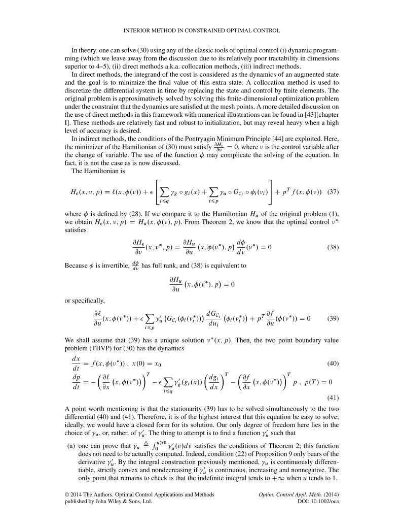
at this point.. We see that in this example we have been able to implement thepoints a) and b) described in Section 7 when studying the solving of the stationarity (39).

Figure 2. Histories of optimal altitude for decreasing values of �.

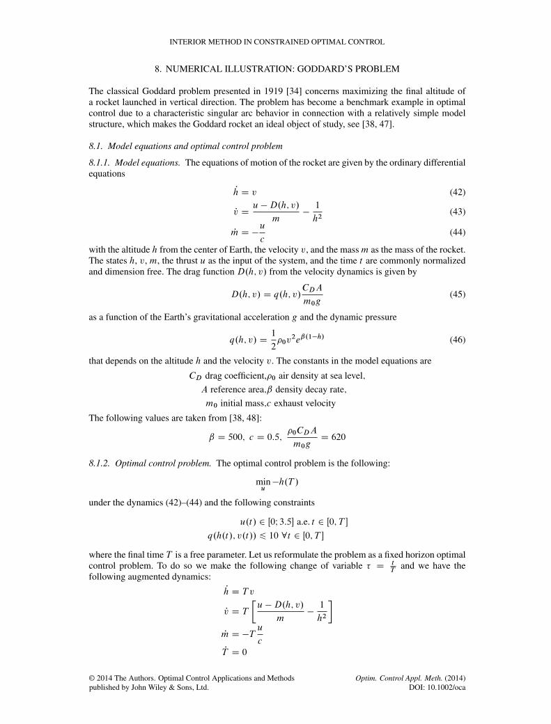
Figure 3. Histories of optimal thrust for decreasing values of �.




Equation (47) then has an analytical solution:

�� D sinh�1��T

�

�pvm�pm

c

�

The problem solving is initialized with constant values of the variables as follows:

h.t/ D 1 v.t/ D 0:2 m.t/ D 1 T D 0:5ph.t/ D 0 pv.t/ D 1 pm.t/ D 0 pT .t/ D 0

The sequence .�n/ is initialized with �0 D 10�2, the parameter ng from 9 is set at ng D 1:1.To solve the problem we use the MATLAB software bvp5c. The source for this example is avail-able at [49]. Other numerical examples, notably with a two dimensional convex control set, can befound in [43].

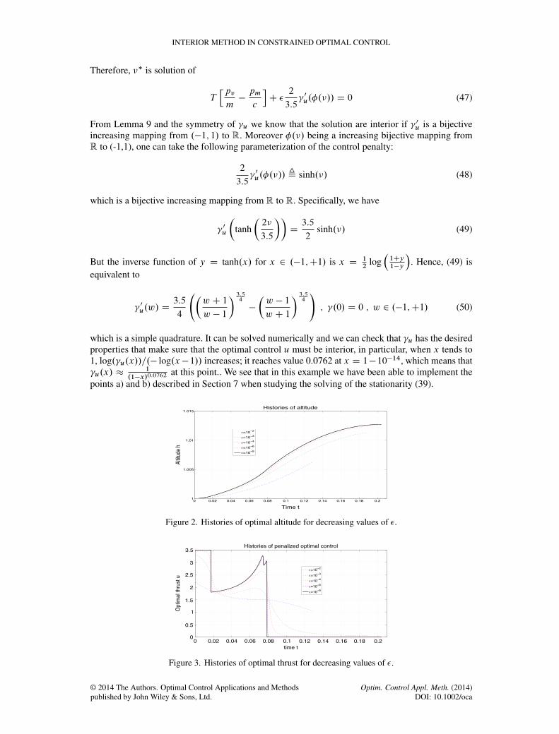
Figure 4. Histories of optimal dynamic pressure for decreasing values of �.

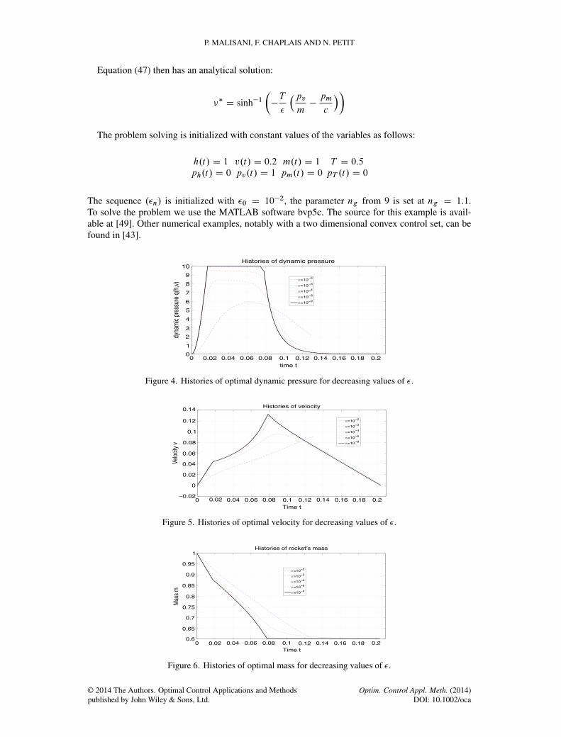
Figure 5. Histories of optimal velocity for decreasing values of �.

Figure 6. Histories of optimal mass for decreasing values of �.




8.2. Results

From Figures 2 to 6 histories of state variables, thrust and state constraints are given for decreas-ing values of the parameter �. One can see that these solutions are similar to those given in [38].Moreover, the optimal final time and the optimal value of the criterion are the following:

T D 0:20405546 I h.T / D 1:01271747

9. CONCLUSION

We have constructively exhibited three classes of penalized optimal control problems whose optimalcosts converge to the optimal control of a given optimal control problem with state and control con-straints. Under classical convexity assumptions, we also have convergence of the control and statetoward the optimal control and state of the original problem.

A notable feature of all of these penalized problems is that the state penalty is sufficient to guar-antee that the state constraints are strictly satisfied; thus they do not need to be specified in the penal-ized problem. By adding a control penalty, we ensure that the second problem has an optimal controlwhich is in the interior of its constraint set; therefore, it must satisfy a stationarity condition on theHamiltonian. By making the most of this interiority property, we can finally operate a invertiblechange of variable on the control which defines an unconstrained penalized optimal control prob-lem. Solving this unconstrained problem and recovering the original control by the inverse transformyields convergence of the cost and, under suitable assumptions, of the control.

Finally, we have observed on all of our numerical examples that the co-states exhibit a conver-gent behavior; moreover, singularities appear gradually at the points where the theory predicts theyshould appear, typically, entry and exit points of singular arcs. Proving the convergence of the co-states toward the co-states of the original problem is a challenging task. If it was achieved, thesemethods would provide an automatic method for computing the co-states and the location of theirsingularities in the original problem.

APPENDIX A: RECALL ON INTERIOR POINT METHODS

A.1. A result by Fiacco and McCormick

We recall a seminal result originally published in [50, 51] because of its general interest in thepresented context and the simplicity of its proof. The interior methods are based on this result. Weconsider an abstract control setE with two subsetsR and S , on which a functional J is defined, withvalues in R. We wish to minimize J over the set R. This task may prove to be too difficult as-is, andinstead, one can choose to solve a sequence of (easier) problems indexed by a positive parameter �

minu2S

J.u/C �G.u/ (51)

where G is defined on S (defined later-on) with nonnegative values in R.

Theorem 5 (Fiacco, McCormick)We assume that problem (51) admits at least a minimizer u�.�/ that belongs to R \ S . Let v0 Dinfu2R J.u/. We assume that v0 is finite and that there exists a minimizing sequence in S for whichJ converges to v0, that is, for any ! > 0 there exists s.!/ 2 S such that v0 6 J.s.!// 6 v0 C !.Then

A lim�#0 J.u�.�// D v0 D infu2R J.u/

B lim�#0 �G.u�.�// D 0

Proof: (inspired from [50, 51])Let ! > 0 an arbitrary small number , and define �1 D !=G.s.!//, (if G.s.!// D 0, we take




�1 D 1). Then we have

J.s.!//C �1G.s.!// 6 v0 C 2!

Consider now any � such that 0 < � 6 �1. We have the following inequalities

v0 6 J.u�.�//C �G.u�.�//D min

u2SJ.u/C �G.u/

6 J.s.!//C �G.s.!//6 J.s.!//C �1G.s.!//6 v0 C 2!

This proves that lim�#0 J.u�.�// C �G.u�.�// D v0. Because G is nonnegative and J.u�.�// is

lower bounded by v0, this proves the limits A and B in the theorem. �

Monotonicity For the sake of completeness, we mention another result that can be found in [50]; adetailed proof of it can be found in [40].

Proposition 12J.u�.�// decreases when � decreases, and G.u�.�// increases when � decreases.

A.2. Interior point methods

Without giving details on the relevant topology, IPMs take for S the interior of the set R, and wehave S � R. If, for instance, E is a Hilbert space and if J C �G has a minimum in the open setS , then it is characterized by the conditions of a free extremum, which are much simpler to solvethan the optimality conditions for the original problem. The challenge is to design the penalty Gsuch that the penalized problem (51) reaches a minimum on the open set S . This is, in general,achieved by using suitable penalties that tends to C1 when u tends to the boundary of R. Thesecond assumption is that the infimum of J over R can be reached by elements of S , that is, theinterior of S . This can be achieved by assuming that R is convex.

In these settings, Theorem 5 proves the convergence of J.u�.�// toward the optimal value v0.The convergence of u�.�/ toward a minimizer of J over R can be then proven by arguments totallyunrelated to the IPM, typically by using convex analysis.

APPENDIX B: CONVEXITY OF THE SET C

C is convex, so U is convex. Let us prove that U is closed. To simplify the proof, we shall use thegauge function on C; the properties of gauge functions are detailed in Section 4.1 and are quitegeneral and independent of the other results presented in this paper. If GC is the gauge function ofC, it is continuous and a vector u belongs to C if and only if GC.u/ 6 1. For u 2 L1Œ0; T �, define

G1C .u/ D sup esst2Œ0;T �GC.u.t//

Then, clearly u 2 U if and only if G1C .u/ 6 1. Moreover, it is easy to check that G1C is continuousfor the sup norm. This proves that U is closed for the sup norm.

APPENDIX C: PROPERTIES OFı

XAD

The set of points that verify gi .x/ < 0 is open because gi is continuous. As a consequence,ı

X ad isa finite intersection of open sets and is thus open.




To prove the density result, consider x 2 Xad and let ˛ 2 .0; 1/. Because gi is convex and

x0 2ı

X ad, we have

gi .˛x0 C .1 � ˛/x/ 6 ˛gi .x0/C .1 � ˛/gi .x/ 6 ˛gi .x0/ < 0

By letting ˛ tend to 0, this proves thatı

X ad is dense in Xad.

Proposition 13For all u 2 U , the maximal solution xu of the dynamics (2) is defined on Œ0; T � and xu is bounded bya constant that depends only on x0 andD. Moreover, the mapping that maps u 2 U to the trajectoryxu 2 C 0.Œ0; T �;Rn/ is Lipschitz when U is equipped with the L1 or L1 norm. As a consequence,the functional J.u/ is Lipschitz over U when equipped with one of these norms.

ProofConsider xu as the maximal solution of (2). The use of the Gronwall Lemma ([52] p. 651) forthe dynamics shows that xu is bounded on its interval of definition. Because f is continuouslydifferentiable, the boundedness of u 2 U and of xu implies that the derivatives of f are boundedwhen u 2 U . Consider now two controls u and v in U . Using the Gronwall Lemma on xu � xv

shows that its dynamics is sub-linear with respect to xu�xv and u� v with a zero initial condition,which proves the regularity of xu with respect to u, both in the L1 and L1 norms. �

APPENDIX D: PROOF OF PROPOSITION 2

The result is trivial if ˛ D 0. We now assume ˛ > 0. From Proposition 13 given earlier inAppendix C and from the continuous differentiability of the gi , there exists a constant � such that,for all u 2 U and any s; t in Œ0; T �

jgi .xu.t// � gi .x

u.s//j 6 �jt � sj (52)

Let ˛ 2 .0; ˛0� and u 2 U n X strict. Then, there exists an index i for which gi .xu/ reaches 0 inŒ0; T �. Remember that gi .x0/ D �˛0 < 0. Denote by t2 the first instant at which gi .xu/ D 0 andt1 D max¹s < t2 s.t. gi .xu.s// D �˛ 2 Œ�˛0; 0/º. From (52), we have

˛ D gi .xu.t2// � gi .x

u.t1// 6 �jt2 � t1j D �.t2 � t1/

As a consequence, we have .t2 � t1/ > ˛=� . Then, we have

�˛ 6 gi .xu.s// 6 0 8s 2 Œt1; t2�

and hence �gi .u; ˛/ > t2 � t1 > ˛=� . This concludes the proof.

APPENDIX E: PROOF OF PROPOSITION 4

There exists two closed ball BN and BM such that

BN � C � BM

with strict inclusions. We define N > 0 (respectively M > 0) as the radius of the ball BN (respec-tively BM ).Now, if u D 0, then GC.u/ is well defined and is equal to 0. We now assume that u ¤ 0.Then

Nu

kuk2 C




because it has norm N ; as a consequence u 2 kukN

C which proves that GC.u/ is well defined andupper bounded by kuk

N. This proves property a) and the right hand side inequality of (14).

On the other side, if u ¤ 0 then

Mu

kuk… C

because its norm is M . As a consequence u … kukM

C, and u … C if 6 kukM

. Then, GC.u/ is lowerbounded by kuk

M; this also holds if u D 0. This end the proof of property b).

The positive homogeneity of the gauge is trivial; because it is sub-additive [36], it is convex. Thecontinuity comes from the fact that it is convex and lower and upper bounded in the neighborhoodof any point. This proves properties c) and d).

The Dini derivative at 0 is obtained by observing that GC.0/ D 0 and that GC.hd/hD GC.d/ if

h > 0. We see that there exists a directional derivative at 0 along the direction d if and only if theDini derivatives along the directions d and �d are equal, which is equivalent to the intersection of Cwith the line directed by d being symmetrical with respect to 0. This proves property e). Note that,if this symmetry holds for all directions, then the gauge function is a norm.

Let us prove property f ). Because the boundary is continuously differentiable, there exists acontinuously differentiable function ' W Rm 7! R such that @C D ¹u s.t. '.u/ D 0º. For allu 2 Rm n ¹0º, u 2 @C , g.u; / , '.u/ D 0. In the following, for any u 2 Rm n ¹0º, we con-sider such that g.u; / D 0. From the convexity of C and because 0 belongs to the interior of C,one has @g

@�.u; / D< r'.u/; u >¤ 0 for all u 2 Rm n ¹0º. Using the implicit function theorem,

there exits .�˛; ˛/ � R and U a neighborhood of u and a C 1 function h W U 7! .�˛; ˛/ such that8� 2 . � ˛; C ˛/ and 8v 2 U g.v; �/ D 0 , � D h.v/ D GC.v/. Therefore, GC is C 1 onRm n ¹0º. This proves f ).

Let us now prove property g). We first verify easily that u 2 C if and only if GC.u/ 6 1 becauseC is closed [36]. Moreover, for any u ¤ 0, the intersection of C with the half axis directed by u isthe segment

h0; uGC.u/

ibecause C is closed and GC.u/ > 0 [36]. As a consequence, GC.u/ D 1

implies that u is in the boundary of C. Conversely, if GC.u/ D 1 � 2˛ with ˛ > 0, because GC iscontinuous, there exists a neighborhood V of u where GC.u/ 6 1 � ˛. For all elements v 2 V , theintersection of C with the half-axis directed by v contains

�0; v1�˛

�. This implies the existence of a

neighborhood of u that is included in C, and hence that u is interior to C. Similarly, if GC.u/ > 1,u … C, one shows the existence of a neighborhood V of u and of ˛ > 0 such that the intersection ofC with the half-axis directed by v 2 V is included in

�0; v1C˛

�. Therefore, u belongs to the exterior

of C. A consequence of all this is that the boundary of C is exactly defined byGC.u/ D 1, its interiorby GC.u/ < 1, and its exterior by GC.u/ > 1. This ends the proof.

APPENDIX F: PROOF OF PROPOSITION 8

To exhibit an upper bound on the variation of the cost, this variation is split into three additive terms,bounding respectively the variation of the original cost, of the integral of the state penalty, and theintegral of the control penalty.

Define M D maxi Mi . From §4.4, one readily sees that

ku � vkL1 6 2˛M�u.˛/

We now proceed to establish bounds for the various terms.

F.1. Upper bound on the variation of the original cost

Here, an upper bound on jR T0 `.x

v; v/ � `.xu; u/dt j is exhibited. It is noted K`. From Proposition13, there exist ƒ > 0 such that




K` 6 ƒZ T

0

kxv � xukL1C k v.t/ � u.t/ k dt 6 ƒ ŒCT C 1� kv � ukL1

6 ƒŒCT C 1�2˛M�u.˛/

Define Ul D ƒ.CT C 1/2M ; then

Kl 6 Ul˛�u.˛/ (53)

F.2. Upper bound on the variation of the state penalty

Note K�g , �PqiD1

R T0 �g ı gi .x

v/ � �g ı gi .xu/dt . Because �g is increasing, the integrand

is positive only when gi .xv.t// > gi .xu.t//. Yet, from the construction of v in (19), one has

maxi gi .xv.t// 6 �ˇ0 for all t 2 Œ0; T �. Using the convexity of �g , and the fact that gi is Lipschitzwith constant Kg on X ad, one obtains

K�g 6 �qXiD1

Zgi .x

v.t//>gi .xu.t//�g ı gi .x

v/ � �g ı gi .xu/dt

6 �qXiD1

Zgi .x

v.t//>gi .xu.t//jgi .x

u.t// � gi .xv.t//j� 0g.gi .x

v.t///dt

6 �qZ T

0

Kgkxu � xvk1�

0g.�ˇ0/dt

6 �qTKgCku � vkL1� 0g.�ˇ0/6 �qTKgC� 0g.�ˇ0/2˛M�u.˛/ (54)

Define

Ug.�/ D �qTKgC�0g.�ˇ0/2M

then, we have

K�g 6 Ug.�/˛�u.˛/

F.3. Upper bound on the variation of the control penalty

There, we aim at getting a negative variation so that, as a whole, the cost is decreased when replacingu by v.

Define

Ku , �pXiD1

Z T

0

�u�GCi .vi .t//

�� u

�GCi .ui .t//

�dt:

From the construction of v (19), we know that GCi .vi .t// 6 GCi .ui .t//. Because �u is non-decreasing, this proves that the integral is negative or null. Moreover, because ui D vi whenGCi .ui / < 1 � ˛i , we have

Ku D �

pXiD1

ZGCi .ui />1�˛i

�u�GCi .vi .t//

�� u

�GCi .ui .t//

�dt




Using the convexity of �u, one has

Ku 6 ��pXiD1

ZGCi .ui />1�˛

k GCi .vi / �GCi .ui / kL1 � 0u�GCi .vi .t//

�dt

D ��

pXiD1

ZGCi .ui />1�˛

k GCi .vi / �GCi .ui / kL1 � 0u�.1 � 2˛/GCi .ui .t//

�dt

6 ��pXiD1

ZGCi .ui />1�˛

k GCi .vi / �GCi .ui / kL1 � 0u Œ.1 � 2˛/.1 � ˛/� dt

6 ��pXiD1

ZGCi .ui />1�˛

k GCi .vi / �GCi .ui / kL1 � 0u.1 � 3˛/dt

6 ��pXiD1

ZGCi .ui />1�˛

2˛ k GCi .ui / kL1 � 0u.1 � 3˛/dt

6 ��pXiD1

ZGCi .ui />1�˛

2˛.1 � ˛/� 0u.1 � 3˛/dt

D ��

pXiD1

�ui .˛/˛�0u.1 � 3˛/

6 ��˛� 0u.1 � 3˛/�u.˛/ (55)

F.4. An upper bound on K.u2; �/ �K.u1; �/

Gathering (53)–(55), we obtain

K.v; �/ �K.u; �/ 6 ˛�U` C Ug.�/ � ��

0u.1 � 3˛/

��u.˛/

This concludes the proof of Proposition 8. One can see that the variation is negative for ˛ smallenough if � 0u.1 � ˛/ tends toC1 when ˛ tends to 0.

APPENDIX G: PROOF OF PROPOSITION 10

Let us define f W Bk:k.0; 1/ 7! int.C/ as

f . / D

8<:0 if D 0k k

GC. / otherwise

The differentiability of the function f on Rm n ¹0º stems from the differentiability of both k:k andGC . The continuity at 0 stems from (14). Its inverse is given by the following function

f �1. / D

8<:0 if D 0

GC. /

k kotherwise

Similarly, the differentiability of the function f �1 on Rm n ¹0º stems from the differentiability ofboth k:k and GC . The continuity at 0 stems from (14).




Using (27), the function

�.�/ , f ı .�/ D tanh.k � k/ ŒGC ı .�/��1 tanh.k � k/

�

k � k

D tanh2.k�k/ ŒGC ı .�/��1 �

k�k

maps Rm into int.C/. This mapping being the composition of two homeomorphism not differentiableonly in 0, � is a homeomorphism differentiable everywhere except at 0. The inverse function Wint.C/ 7! Rm is the following:

.u/ , �1 ı f �1.u/ D atanh.GC.u//u

k u k

This concludes the proof.

APPENDIX H: REMARKS ON SOLUTION ALGORITHMS USINGSATURATION FUNCTIONS

We rely on the routines bvp4c or bvp5c for solving the TBVPs. We shall denote them by bvpxc.

Values of � We have first to define a sequence of values for � for which we shall solve the penalizedproblems. A practical choice is to choose a geometric progression using

EPS=logspace(a,b,n)The initial exponent a should not be too small in order for bvpxc to initialize correctly. Indeed, if

� is very small, we are close to the solution of the optimal problem; in particular, we have observedthat the co-states converge numerically to singular functions (as expected from the theory). Thismeans that if � is small at the start, for bvpxc to succeed, it must use a very fine mesh refinementin the neighborhood of the singularities of the co-states. Because, at the beginning of the algorithm,we have no idea where the singularities occur, this is a very difficult task. This is why we start with� not too small. The number n of values for � is a tradeoff between two considerations

� if n is large, then we are close to a continuation method, as we feed the result of the previousiteration as an initial guess for the next iteration. This means that the collocation algorithmwill be faster because the dynamics of the two iterations are close, and hence, the initial guesswill be a good one. In particular, the mesh that is used for the initial guess will yield suitablerefinements in the neighborhood of the ‘singularities’ of the costate when � is small.� on the other hand, a large n means a large number of iterations in the algorithm. In practice,

beyond a certain value, increasing n only increases the computation time without improvingthe results.

The final exponent b essentially depends on the computing power of your machine. Of course nmust be increased if b is increased. We shall denote by �i , i D 1; : : : ; n the sequence previouslydefined.

Collocation options We must also provide a maximum number of mesh-points and a (relativeand/or absolute) error for the collocation method. It is mainly a trial and error process; it is advisedto try a small number of meshpoints and a reasonable tolerance first. Note that, beyond a certainvalue, increasing the possible number of mesh-points may be counterproductive. It is also possibleto adapt these parameters to �. A reasonable choice is to increase the possible number of mesh-points as � decreases.

Initial guess An initial guess Ix;1 and Ip;1 must be given for the state and costate. The important

point is that Ix;1 must satisfy Ix;1Œk� 2ı

X ad for all the indices k. There is no requirement on the




costate Ip;1, except that its final value is zero. The time samples can be arithmetically distributed atthis stage, because for � not very small, the solving of (40) and (41) should not be stiff.

Iterations Using the initial guess Ix;i and Ip;i , use bvpxc to solve the TBVP (40) and (41) for� D �i , with the settings described in the initialization step. Let .xi ; pi / the output of the solver.

If i < n, define .Ix;iC1; Ip;iC1/ D .xi ; pi /, increment i and loop into the iteration step.If i D n, the state produced by the algorithm is xn, the costate is pn, and the control is obtained

by solving (39) with respect to the unknown �.��/. The iteration is stopped there.Remark: when doing .Ix;iC1; Ip;iC1/ D .xi ; pi /, the time samples that are produced by bvpxc

are passed as an initial mesh for the next iteration. This means that, if, for index i , the singu-larities begin to appear in pi then the mesh is adapted to these singularities, and, if the distancebetween two successive values of � is not too big, it will provide a suitable initial mesh for thecollocation method.

REFERENCES

1. Murray RM, Hauser J, Jadbabaie A, Milam MB, Petit N, Dunbar WB, Franz R. Online control customization viaoptimization-based control. In Software-Enabled Control, Information Technology for Dynamical Systems, Samad T,Balas G (eds). John Wiley & Sons, Inc.: Hoboken, NJ, USA, 2003; 149–174.

2. Byrd RH, Nocedal J, Waltz RA. KNITRO: An Integrated Package for Nonlinear Optimization. In Large-ScaleNonlinear Optimization, di Pillo G, Roma M (eds). Springer Verlag, 2006; 35–59.

3. Wright MH. The interior-point revolution in optimization: History, recent developments, and lasting consequences.Bulletin (New Series) of the American Mathematical Society 2004; 42:39–56.

4. Forsgren A, Gill PE, Wright MH. Interior methods for nonlinear optimization. SIAM Review 2002; 4(4):525–597.5. Hauser J, Saccon A. A barrier function method for the optimization of trajectory functionals with constraints. 45th

IEEE Conference on Decision and Control, San Diego, 2006; 864–869.6. Fabien BC. An extended penalty function approach to the numerical solution of constrained optimal control problems.

Optimal Control Applications and Methods 1996; 17(5):341–355.7. Xing AQ, Chen ZH, Wang CL, Yao YY. Exact penalty function approach to constrained optimal control problems.

Optimal Control Applications and Methods 1989; 10(2):173–180.8. Xing A-Q, Wang C-L. Applications of the exterior penalty method in constrained optimal control problems. Optimal

Control Applications and Methods 1989; 10(4):333–345.9. Bryson AE, Ho YC. Applied Optimal Control. Ginn and Company: Waltham, MA, 1969.

10. Bonnans JF, Hermant A. Stability and sensitivity analysis for optimal control problems with a first-order stateconstraint and application to continuation methods. ESAIM: Control, Optimisation and Calculus of Variations 2008;14(4):825–863.

11. Hartl R, Sethi S, Vickson R. A survey of the maximum principles for optimal control problems with state constraints.SIAM Review 1995; 37(2):181–218.

12. Hargraves C, Paris S. Direct optimization using nonlinear programming and collocation. AIAA Journal of Guidance,Control and Dynamics 1987; 10:338–342.

13. Kojima A, Morari M. LQ control for constrained continuous-time systems. Automatica 2004; 40:1143–1155.14. Yuz J, Goodwin G, Feuer A, De Doná J. Control of constrained linear systems using fast sampling rates. Systems and

Control Letters 2005; 54:981–990.15. Bemporad A, Casavol A, Mosca E. A predictive reference governor for constrained control systems. Computers in

Industry 1998; 36:55–64.16. Bemporad A, Morari M, Dua V, Pisikopoulos EN. The explicit linear quadratic regulator for constrained systems.

Automatica 2002; 38:3–20.17. Petit N, Milam M, Murray RM. Inversion based constrained trajectory optimization. IFAC Symposium on Nonlinear

Control Systems Design, St. Petersburg, 2001.18. Bhattacharya R. OPTRAGEN: A Matlab toolbox for optimal trajectory generation. 45th IEEE Conference on

Decision and Control, San Diego, 2006; 6832–6836.19. Ross IM, Fahroo F. Pseudospectral knotting methods for solving nonsmooth optimal control problems. AIAA Journal

of Guidance, Control and Dynamics 2004; 27(3):397–405.20. Wright SJ. Interior point methods for optimal control of discrete time systems. Journal of Optimization Theory and

Applications 1993; 77:161–187.21. Vicente LN. On interior-point Newton algorithms for discretized optimal control problems with state constraints.

Optimization Methods and Software 1998; 8:249–275.22. Leibfritz F, Sachs EW. Inexact SQP interior point methods and large scale optimal control problems. SIAM Journal

on Control and Optimization 1999; 38:272–293.23. Jockenhövel T, Lorenz TB, Wächter A. Dynamic optimization of the Tennessee Eastman process using the

Optcontrolcentre. Computers and Chemical Engineering 2003; 27:1513–1531.




24. Yu C, Li B, Loxton RC, Teo KL. Optimal discrete-valued control computation. Journal of Global Optimization 2013;56(2):503–518.

25. Yu C, Teo KL, Zhang L, Bai Y. A new exact penalty function method for continuous inequality constrainedoptimization problems. Journal of Industrial and Management Optimization (JIMO) 2010; 6(4):895–910.

26. Li B, Yu C, Teo KL, Duan G-R. An exact penalty function method for continuous inequality constrained optimalcontrol problem. Journal of Optimization Theory and Applications 2011; 151(2):260–291.

27. Jiang C, Lin Q, Yu C, Teo KL, Duan G-R. An exact penalty method for free terminal time optimal control problemwith continuous inequality constraints. Journal of Optimization Theory and Applications 2012; 154(1):30–53.

28. Loxton RC, Teo KL, Rehbock V, Yiu KFC. Optimal control problems with a continuous inequality constraint on thestate and the control. Automatica 2009; 45(10):2250–2257.

29. Gerdts M, Kunkel M. A nonsmooth Newton’s method for discretized optimal control problems with state and controlconstraints. Journal of Industrial and Management Optimization (JIMO) 2008; 4(2):247–270.

30. Bonnans JF, Guilbaud T. Using logarithmic penalties in the shooting algorithm for optimal control problems. OptimalControl Applications and Methods 2003; 24:257–278.

31. Malisani P, Chaplais F, Petit N. Design of penalty functions for optimal control of linear dynamical systems understate and input constraints. 50th IEEE Conference on Decision and Control and European Control Conference,Orlando, 2011; 6697–6704.

32. Malisani P, Chaplais F, Petit N. A constructive interior penalty method for non linear optimal control problems withstate and input constraints. Proceedings of IEEE American Control Conference, Montreal, 2012; 2669–2676.

33. Malisani P, Chaplais F, Petit N. A fully unconstrained interior point algorithm for multivariable state and inputconstrained optimal control problems. European Congress on Computational Methods in Applied Sciences andEngineering, Vienna, 2012.

34. Goddard RH. A Method for Reaching Extreme Altitudes. Smithsonian Int. Misc. Collections 71: Washington, 1919.35. Kolmogorov AN, Fomin SV. Elements of the Theory of Functions and Functional Analysis. Dover Publications:

Mineloa, New York, 1999.36. Schwartz L. Analyse Hilbertienne. Ecole Polytechnique: Palaiseau, France, 1978.37. Graichen K, Petit N, Kugi A. Transformation of optimal control problems with a state constraint avoiding interior

boundary conditions. Proceedings of the 47th IEEE Conference on Decision and Control, Cancun, 2008; 913–920.38. Graichen K, Petit N. Solving the Goddard problem with thrust and dynamic pressure constraints using saturation

functions. Proceedings of the 2008 IFAC World Congress, Seoul, 2008; 14301–14306.39. Graichen K, Petit N. Constructive methods for initialization and handling mixed state-input constraints in optimal

control. Journal Of Guidance, Control, and Dynamics 2008; 31(5):1334–1343.40. Graichen K, Petit N. Incorporating a class of constraints into the dynamics of optimal control problems. Optimal

Control Applications and Methods 2009; 30(6):537–561.41. Graichen K, Kugi A, Petit N, Chaplais F. Handling constraints in optimal control with saturation functions and

system extension. Systems and Control Letters 2010; 59(11):671–679.42. Graichen K. Feedforward control design for finite-time transition problems of nonlinear systems with input and

output constraints. Ph.D. Thesis, Universität Stuttgart, 2006.43. Malisani P. Dynamic control of energy in buildings using constrained optimal control by interior penalty. Ph.D.

Thesis, Mines ParisTech, Paris, France, September 2012. (Available from: http://pastel.archives-ouvertes.fr/docs/00/74/00/44/PDF/Malisani.pdf) [Accessed on 25 August 2014].

44. Pontryagin LS, Boltyanskii VG, Gamkrelidze RV, Mishchenko EF. The Mathematical Theory of Optimal Processes.Interscience Publishers John Wiley & Sons, Inc.: New York, London, 1962.

45. Shampine L, Kierzenka J, Reichelt M. Solving boundary value problems for ordinary differential equations in matlabwith bvp4c, 2000. (Available from: http://www.mathworks.com/bvp_tutorial) [Accessed on 25 August 2014].

46. BOCOP v1.03 User Guide. INRIA: France, 2012.47. Milam MB. Real-time optimal trajectory generation for constrained dynamical systems. Ph.D. Thesis, California

Institute of Technology, Pasadena, USA, 2003.48. Seywald H. Trajectory optimization based on differential inclusion. AIAA Journal of Guidance, Control and

Dynamics 1994; 17:480–487.49. Malisani P. Source code for solving goddard’s problem, 2013. (Available from: http://cas.ensmp.fr/~petit/

code_optimisation_PM/main_goddard.m) [Accessed on 25 August 2014].50. Fiacco AV, McCormick GP. The sequential unconstrained minimization technique for nonlinear programming, a

primal-dual method. Management Science 1964; 10(2):360–366.51. Fiacco AV, McCormick GP. Nonlinear Programming: Sequential Unconstrained Minimization Techniques. Wiley:

New York, 1968.52. Khalil H. Nonlinear Systems. Prentice Hall, 2002.



http://pastel.archives-ouvertes.fr/docs/00/74/00/44/PDF/Malisani.pdf

http://pastel.archives-ouvertes.fr/docs/00/74/00/44/PDF/Malisani.pdf

http://www.mathworks.com/bvp_tutorial

http://cas.ensmp.fr/~petit/code_optimisation_PM/main_goddard.m

http://cas.ensmp.fr/~petit/code_optimisation_PM/main_goddard.m

an interior penalty method for optimal control problems with...

Documents