1 dynamics and solutions to some control problems for...
TRANSCRIPT

1
Dynamics and solutions to some control problemsfor water-tank systems
Nicolas Petit , Pierre Rouchon
Abstract
We consider a tank containing a fluid. The tank is subjected to directly controlled translations and rotations. The fluid motionis described by linearized wave equations under shallow water approximations. For irrotational flows, a new variational formulation ofSaint-Venant equations is proposed. This provides a simple method to establish the equations when the tank is moving. Several controlconfigurations are studied: one and two horizontal dimensions; tank geometries (straight and non-straight bottom, rectangular and circularshapes), tank motions (horizontal translations with and without rotations). For each configuration we prove that the linear approximation issteady-state controllable and provide a simple and flatness-based algorithm for computing the steering open-loop control. These algorithmsrely on operational calculus. They lead to second order equations in space variables whose fundamental solutions define delay operatorscorresponding to convolutions with compact support kernels. For each configurations several controllability open-problems are proposed andmotivated.
Keywords:. Wave equations, boundary control, flatness, controllability, motion planning, delay operators.
Introduction
The following study is derived from an industrial problem for which tanks filled with liquid are to be moved todifferent steady-state workbenches as fast as possible. For such start and stop motions, the fluid mass has a significantcontribution in the dynamics of the whole system. Several recent publications deal with this question, see, for example,[1], [2], [3], [4], [5]. This paper is a first attempt to base the control design on wave equations describing the fluid surfacedynamics .
We concentrate on finding open-loop tank trajectories such that if the liquid is initially at rest then it returns to restwhen the tank stops. This is a typical motion planning problem: finding open-loop control steering in finite time fromone steady-state to another one. For finite dimensional systems, flatness based methods [6], [7] are very efficient to solvethis problem. In [8], [9], [10], [11], [12], [13], infinite dimensional extensions are proposed for several systems describedby partial differential equations with boundary control. We employ such a “flatness based” methodology, working onphysical models of the system and we establish several controllability results: positive results consider exact steady-statecontrollability in finite time T , i.e., proving that there exists a control [0, T ] t → u(t) steering the system from anysteady-state to any other one, on the other hand negative results describe the lack of approximate controllability.
The first contribution of the paper consists of models. The major modelling difficulty lies in the fact that the fluidsurface is unknown. A “rigorous” modelling involving Euler or Navier-Stoke equations with free surface boundaries isout of reach. Thus we restrict our study to classical modelling based on shallow water approximation [14]. Even for suchrestrictive modelling, the motion equations are not so simple to derive when the tank is moving. Thus in a first step, wepropose a variational formulation of the Saint-Venant equations for irrotational flows and fixed tank: their solutions areextremal of the action under the constraint formed by the mass conservation equation. Then, when the tank is moving,we derive a similar formulation by adding the contribution of the tank motion in the kinetic and potential energy andproceed as before to get the dynamics.
The second contribution is relative to motion planning. The Saint-Venant equations are nonlinear hyperbolic equa-tions. Only few results are available concerning their nonlinear stability, stabilization and controllability (see, e.g.,[15], [16] and a recent result in [17]). Preliminary results [18] sketched in appendix lead us to thinking that, whenused properly, linearized Saint-Venant equations can be an insighful approximation for motion planning purposes. Werestrict our study to such linearized wave equations and show how to obtain open-loop control algorithms that arecomputationally straightforward. They are derived from formulas presented in lemmas 3, 4, 5 and 6 and are based onsymbolic computations and involve operational calculus, Bessel functions, and Paley-Wiener theorem.
We would like to emphasize that although wave equations with Neuman boundary control have been intensivelystudied and many precise and general results are available on their controllability and stabilization (see, e.g., [19], [20],[21], [22], [23]), the classical results do not apply in a simple way to the problem presented in this paper. First reason: wehave a linear wave equation controlled via Neuman boundary control but, the control is not distributed on the boundary;even for the simple tank described by system (26), the same control u, the acceleration of the tank, appears at bothedges x = −a and x = a. Second reason: the controlled wave equation is coupled with a double integrator D = u; onehas to control not only the surface waves inside the tank but also the position and velocity of the tank.
N. Petit is with the Centre Automatique et Systemes, Ecole des Mines de Paris, France. Email: [email protected].
P. Rouchon is the director of the Centre Automatique et Systemes, Ecole des Mines de Paris, France. Email: [email protected]
2
The paper is organized as follows. The dynamics of the systems under consideration are the subject of section I.Sections II and III are devoted to control problems for the one-dimensional and two-dimensional cases respectively.
More precisely, in section I we detail the variational formulation: the Saint-Venant equations for a moving tank areestablished. In section II, we consider one-dimensional cases: the translation case with a straight bottom is treatedin details; the non-straight bottom is also addressed; combination of tank translation and rotation are investigated.Section III is devoted to two-dimensional cases: the translation of rectangular and circular tanks are solved; the combi-nation of tank translation and rotation for an arbitrary geometry are also solved. In conclusion, we show that shallowwater approximation is essential to ensure an explicit formulation of the dynamics: a more general modelling with anon-horizontal fluid velocity leads to an implicit formulation, an infinite dimensional analogue of an index one differential-algebraic system. In the appendix we prove a technical lemma devoted to symbolic analysis of the one dimensional waveequations when the speed depends on space: it can be seen as a generalization of d’Alembert formulas. We also recall inappendix some preliminary results and nonlinear simulations based on Godunov scheme for the Saint-Venant equation.
In this paper we pin point several open problems. As far as we know, the techniques presented in this paper give onlypartial answer, if any, in these tricky situations. We hope researchers in this area will welcome these challenges.
Some preliminary results relative to the horizontal translation of a tank in a vertical plane and with a straight bottomcan be found in [18]. A preliminary version of this paper can be found in [24].
I. Variational formulations
The Saint-Venant equations describe the motion of a perfect fluid under gravity g with a free boundary (the shallowwater assumption). We provide a variational formulation of these equations that, up to our knowledge, is new althoughnot surprising (see, e.g., [25], [26], [14]). This variational formulation is interesting: it gives directly the dynamicsequations when the tank is moving (translation and rotation).
A. The one-dimensional cases
A.1 One-dimensional straight bottom fixed tank
-a +a
v(x,t)
x
h(x,t)
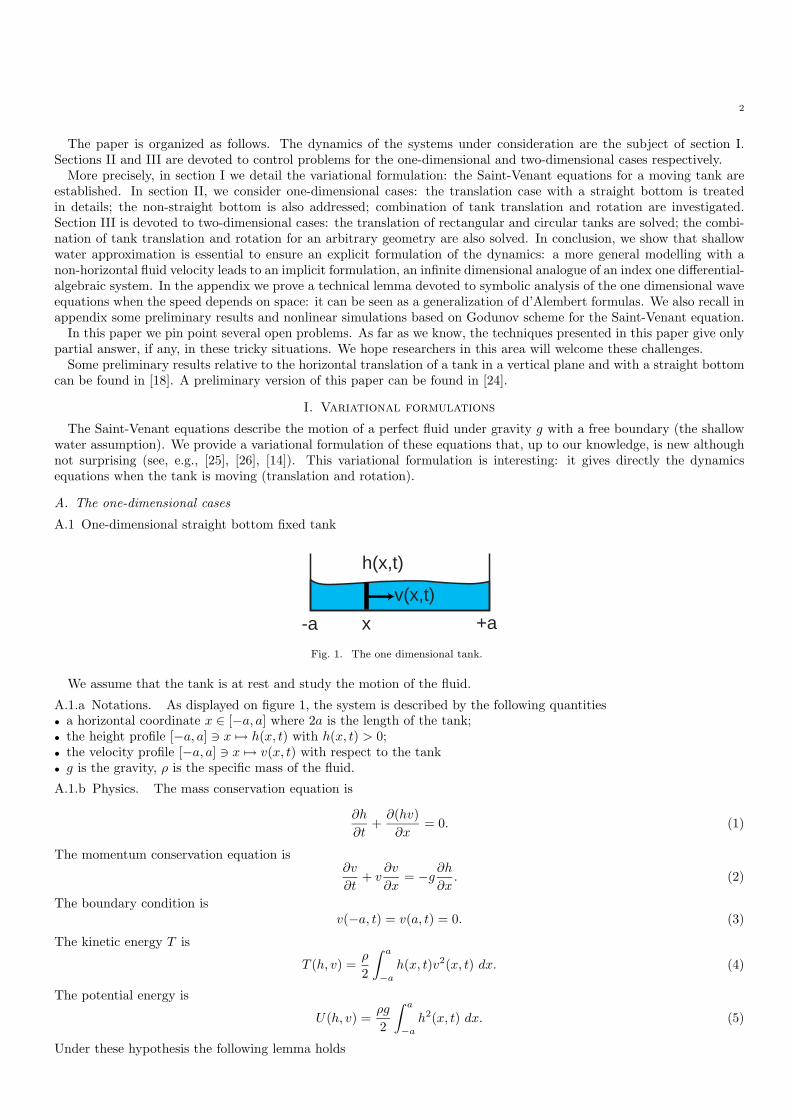
Fig. 1. The one dimensional tank.
We assume that the tank is at rest and study the motion of the fluid.
A.1.a Notations. As displayed on figure 1, the system is described by the following quantities• a horizontal coordinate x ∈ [−a, a] where 2a is the length of the tank;• the height profile [−a, a] x → h(x, t) with h(x, t) > 0;• the velocity profile [−a, a] x → v(x, t) with respect to the tank• g is the gravity, ρ is the specific mass of the fluid.
A.1.b Physics. The mass conservation equation is
∂h
∂t+
∂(hv)∂x
= 0. (1)
The momentum conservation equation is∂v
∂t+ v
∂v
∂x= −g
∂h
∂x. (2)
The boundary condition isv(−a, t) = v(a, t) = 0. (3)
The kinetic energy T is
T (h, v) =ρ
2
∫ a
−a
h(x, t)v2(x, t) dx. (4)
The potential energy is
U(h, v) =ρg
2
∫ a
−a
h2(x, t) dx. (5)
Under these hypothesis the following lemma holds

3
Lemma 1: Take a positive time τ > 0. Equation (2) , i.e. the momentum conservation equation, results from theEuler-Lagrange first-order stationarity conditions deduced from
δ
(∫ τ
0
(T (h, v) − U(h, v)) dt
)= 0 (6)
under the constraints formed by the mass equation (1), the boundary conditions (3) and fixed initial and final valuesfor h and v: h(x, 0) = h0(x), v(x, 0) = v0(t), h(τ, x) = hτ (x), v(τ, x) = vτ (x).
Proof: Denote by λ(x, t) the multiplier associated to the constraint (1) and by L(h, v, λ) the Lagrangian1
L =∫ τ
0
(T (h, v) − U(h, v)) dt +∫ τ
0
∫ a
−a
λ(x, t)(
∂h
∂t+
∂(hv)∂x
)dx dt.
The condition δL = 0 for any small variation δh of h such that δh(x, 0) = δh(x, τ) = 0 yields∫ τ
0
∫ a
−a
[ρ(v2/2 − gh)δh + λ
(∂(δh)
∂t+
∂(vδh)∂x
)]dx dt = 0,
and then thanks to an integration by parts∫ τ
0
∫ a
−a
[ρ(v2/2 − gh) − ∂λ
∂t− v
∂λ
∂x
]δh dx dt = 0.
Thus∂λ
∂t+ v
∂λ
∂x= ρ(v2/2 − gh).
Similarly, variation δv of v such that δv(x, 0) = δv(x, τ) = 0 and δv(−a, t) = δv(a, t) = 0, gives
∂λ
∂x= ρv.
Gathering these last two stationarity equations we get
∂λ
∂t+
ρ
2v2 = −gρh.
A differentiation with respect to x yields∂v
∂t+ v
∂v
∂x= −g
∂h
∂x(7)
which is indeed identical to (2).
A.2 One-dimensional non-straight bottom moving tank
-a
+a
xv(t,x)h(t,x
)
D I
K ki
Ο
Fig. 2. The non-straight bottom tank at rest (right) and in movement (translation and rotation) (left).
We assume that the tank is moving.
1The Lagrangian we use is the classical Lagrangian as used in optimization: the constraints are adjoined with their Lagrange multipliersto the function (or functional) that is minimized.

4
A.2.a Notations. (I, K) is the fixed frame with I horizontal and (ı,k) is the tank frame: ı = cos θI + sin θ K andk = − sin θI + cos θ K.
As displayed on figure 2, the tank motion is described by an horizontal position R+ t → D(t) ∈ R and a rotationangle θ(t) around the horizontal axis orthogonal to the translation axis.
We still assume that the fluid can be described by [−a, a]×R+ (x, t) → h(x, t) and [−a, a]×R+ (x, t) → v(x, t),the velocity with respect to the tank. Notice that the space coordinate x is relative to the tank. Moreover we assumethat the tank bottom is not straight but described by a smooth profile [−a, a] x → b(x) ∈ R. As before g is thegravity, ρ is the specific mass of the fluid.
A.2.b Physics and derivation of the model. The momentum conservation equation is derived from the variationalformulation of lemma 1 with the following kinetic and potential energies (the boundary and constraint conditionsremain unchanged)
T (h, v) =ρ
2
∫ a
−a
h(DI + vı + xθk
)2
dx (8)
U(h, v) = ρg
∫ a
−a
∫ b+h
b
(xı + zk
)· K dz dx. (9)
Denote by λ(x, t) the multiplier associated to the mass conservation constraint and by L the resulting Lagrangian
L(h, v, λ) =∫ τ
0
(T (h, v) − U(h, v)) dt +∫ τ
0
∫ a
−a
λ(x, t)(
∂h
∂t+
∂(hv)∂x
)dx dt.
Stationary condition of L with respect to any small variation δv of v such that δv = 0 for t = 0, τ and x ∈ −a, a,yields
∂λ
∂x= ρ(D cos θ + v). (10)
Stationary condition of L with respect to any small variation δh of h such that δh = 0 for t = 0, τ yields
∂λ
∂t+ v
∂λ
∂x=
ρ
2
(DI + vı + xθk
)2
− ρg(xı + (b + h)k
)· K. (11)
We differentiate (11) with respect to x and substitute ∂λ∂x by the righthand side of (10). We obtain the momentum
conservation equation for v. The full dynamics are then described by the following set of equations
∂h
∂t+
∂(hv)∂x
= 0
∂v
∂t+ v
∂v
∂x= −D cos θ − g sin θ + xθ2 − g cos θ
∂(b + h)∂x
v(−a, t) = v(a, t) = 0.
(12)
Notice that these equations are indeed invariant under Galilean transformations, i.e. uniform translations, D → D +p1t + p0 with p1 and p0 arbitrary constants.
Assume now that θ is small (θ2a g), that h(x, t) = h(x)+H(x, t), with h(x) = −b(x) > 0 (where is a constant)is the steady-state height profile and with |H| h, and |v|
√gh. Notice that we neither assume θ small nor |D| g.
Up to second order-terms the “linearized” dynamics read
∂H
∂t= −∂(hv)
∂x∂v
∂t= −D cos θ − g sin θ − g cos θ
∂H
∂xv(−a, t) = v(a, t) = 0.
We end up with the following modelModel 1: Elimination of v yields to a wave equation for H
∂2H
∂t2=
∂
∂x
[h
(D cos θ + g sin θ + g cos θ
∂H
∂x
)]
g cos θ∂H
∂x(a, t) = g cos θ
∂H
∂x(−a, t) = −D cos θ − g sin θ
(13)

5
where [−a, a] x → h(x) is the steady-state height profile and h(x, t) = h(x) + H(x, t) is up-to second order terms theliquid height. The control variables are D(t) the horizontal acceleration of the tank, and θ(t) its angular velocity. Atany given time t, [−a, a] x → (H(x, t), ∂H
∂t (x, t)), D(t), D(t) and θ(t) constitute the state of the system.These equations are a good approximation as soon as
θ2a g, |H| h, |v| √
gh.
B. The two-dimensional cases
B.1 Two-dimensional straight bottom fixed tank
Fig. 3. The two-dimensional tank.
B.1.a Notations. As displayed on figure 3, the system is described by the following quantities:• two horizontal coordinates x = (x1, x2) ∈ Ω where Ω is an open bounded connected domain of R2 with smoothboundary ∂Ω;• the height profile Ω x → h(x, t) with h(x, t) > 0;• the velocity profile Ω x → v(x, t) ∈ R2.We assume that the tank is at rest. As usual we denote by ∇ the operator
∇ =( ∂
∂x1∂
∂x2
).
The mass conservation equation is∂h
∂t+ ∇ · (hv) = 0 (14)
where v is the velocity field of coordinates (v1, v2).
B.1.b Physics. The momentum conservation equation is
∂v
∂t+ v · ∇v = −g∇h. (15)
The boundary condition isv · n = 0 on ∂Ω (16)
where n is the normal to ∂Ω.We restrict our study to potential flow v, i.e., solutions of (14,15,16) such that ∇× v = 0. This makes sense since if
the initial velocity profile is irrotational, it remains irrotational
∂(∇× v)∂t
+ ∇× [(∇× v) × v) = 0.
For irrotational v, (15) reads also∂v
∂t+
12∇(v2) = −g∇h.
The kinetic energy T is
T (h,v) =ρ
2
∫Ω
h(x, t)v2(x, t) dx1dx2. (17)
The potential energy is
U(h,v) =ρg
2
∫Ω
h2(x, t) dx1dx2. (18)

6
As for the one dimensional case, we have the following lemmaLemma 2: Take a positive time τ > 0 and consider irrotational solutions of (14,15,16) (∇×v = 0). Then equation (15),
i.e. the momentum conservation equation, results from the Euler-Lagrange first-order stationarity conditions deducedfrom
δ
(∫ τ
0
(T (h,v) − U(h,v)) dt = 0)
(19)
under the constraints formed by the mass conservation equation (14), the boundary conditions (16) and fixed initial andfinal values for h and v, h(x, 0) = h0(x), v(x, 0) = v0(t), h(τ, x) = hτ (x), v(τ, x) = vτ (x).The proof is very similar to the one dimensional one and is left to the reader.
B.2 Two-dimensional non-straight bottom moving tank
In the following we sketch the main steps to derive from lemma 2 the dynamical equations when the tank is movingwith an irrotational velocity profile v.
B.2.a Notations. The fixed frame is denoted by (I1, I2, K) where K is the upwards vertical unit vector. The tankframe is (ı1,ı2,k) where the liquid height is along the k axis. The rotation of the tank is described by the instantaneousrotation vector ω defined by
ı1 = ω ×ı1, ı2 = ω ×ı2, k = ω × k.
Since we are looking for irrotational flows, we will see that, necessarily, ω · k = 0: the tank cannot spin around axis k.The fluid remains described by the height profile Ω x → h(x, t) > 0, where Ω is as before an open bounded connected
domain of R2 with a piecewise smooth boundary ∂Ω, and the velocity profile v(x, t) = v1ı1 + v2ı2 where x = (x1, x2)are Cartesian coordinates along a plane attached to the tank and parallel to (ı1,ı2). We assume that the tank bottom isgiven by the profile Ω x → b(x). We denote by (D1,D2, Z) the coordinates in the fixed frame of the point D attachedto the tank. Vertical acceleration can be included by changing gravity g into g + Z and just considering horizontalmotions for D. Without loss of generality, we assume in the sequel that Z ≡ 0 and
D = D1I1 + D2
I2, D = D1I1 + D2
I2.
Once more, g denotes the gravity and ρ is the specific mass of the fluid.
B.2.b Physics and derivation of the model. With the above notations the kinetic and potential energies are
T (h,v) =ρ
2
∫Ω
h(D + v + ω × (x1ı1 + x2ı2)
)2
dx1dx2 (20)
U(h,v) = ρgZ + ρg
∫Ω
∫ b+h
b
(x1ı1 + x2ı2 + zk
)· K dzdx1dx2. (21)
Denote by λ(x, t) the multiplier associated to the mass conservation constraint and by L the resulting Lagrangian
L(h,v, λ) =∫ τ
0
(T (h,v) − U(h,v)) dt +∫ τ
0
∫Ω
λ(x, t)(
∂h
∂t+ ∇ · (hv)
)dx1dx2 dt.
Stationary condition of L with respect to any small variation δv = δv1ı1 + δv2ı2 of v such that δv = 0 for t = 0, τ andδv · n = 0 for x ∈ ∂Ω, yields
∂λ
∂xσ= ρ
(D + v + ω × (x1ı1 + x2ı2)
)·ıσ, σ = 1, 2. (22)
Stationary condition of L with respect to any small variation δh of h such that δh = 0 for t = 0, τ yields
∂λ
∂t+ v · ∇λ =
ρ
2
(D + v + ω × (x1ı1 + x2ı2)
)2
−ρg(x1ı1 + x2ı2 + (b + h)k
)K.
(23)
According to (22)v · ∇λ = ρv ·
(D + v + ω × (x1ı1 + x2ı2)
).
We then apply ∂∂x1
on (23) and substitute ∂λ∂x1
by the righthand side of (22):
∂v1
∂t+ v · ∂v
∂x1= x2
d(ω · k)dt
+ . . .
. . . +∂
∂x1
(12(ω × (x1ı1 + x2ı2))2 − (D + g K) · (x1ı1 + x2ı2) − g(b + h)k · K
).

7
Similarly we have
∂v2
∂t+ v · ∂v
∂x2= −x1
d(ω · k)dt
+ . . .
. . . +∂
∂x2
(12(ω × (x1ı1 + x2ı2))2 − (D + g K) · (x1ı1 + x2ı2) − g(b + h)k · K
).
This provides the vectorial momentum conservation equation for
∂v
∂t+
12∇v2 =
d(ω · k)dt
(x2ı1 − x1ı2) + . . .
. . . + ∇(
12(ω × (x1ı1 + x2ı2))2 − (D + g K) · (x1ı1 + x2ı2) − g(b + h)k · K
).
v must be kept irrotational to apply lemma 2. Thus we restrict rotations by ω · k ≡ 0.The full dynamics is then described by the following set of equations
∂h
∂t+ ∇ · (hv) = 0
∂v
∂t+
12∇v2 =
12∇ (
(ω × (x1ı1 + x2ı2))2)
+ . . .
. . . + ∇(−(D + g K) · (x1ı1 + x2ı2) − g(b + h)k · K
)v · n = 0 on ∂Ω.
(24)
Assume now that ω is small (ω2a g, where a is the typical size of Ω), that h(x, t) = h(x) + H(x, t), withh(x) = cte − b(x) > 0 is the steady-state height profile and with |H| h, and that |v|
√gh. Up to second
order-terms the “linearized” dynamics read
∂H
∂t= −∇ · (hv)
∂v
∂t=∇
(−(D + g K) · (x1ı1 + x2ı2) − gk · KH
).
We end up with the following modelModel 2: Elimination of v yields to a wave equation for H
∂2H
∂t2= ∇ ·
(h∇
[(D + g K) · (x1ı1 + x2ı2) + gHk · K
])∇
[(D + g K) · (x1ı1 + x2ı2) + gHk · K
]· n = 0 on ∂Ω
(25)
where h(x) is the steady-state height profile and h(x, t) = h(x) + H(x, t) is up-to second order terms the liquid height.The control variables are D the tank acceleration and ω its instantaneous rotation vector (remember that ω · k = 0).
At any given time t, [−a, a] x → (H(x, t), ∂H∂t (x, t)), D(t), D and the three Euler angles defining the orientation of
the tank constitute the state of the system.These equations are a good approximation as soon as
ω2a g, |H| h, ‖v‖ √
gh.
II. Several control problems and their solutions for the one-dimensional linearized model
A. Translation and straight bottom
Model 3: Assume that [−a, a] x → b(x) = 0 and θ = 0. Then [−a, a] x → h(x) is constant and model 1 reads
∂2H
∂t2= hg
∂2H
∂x2
∂H
∂x(a, t) =
∂H
∂x(−a, t) = −u
g
D = u
(26)

8
with (H, ∂H∂t ,D, D) as state and u as control.
The controllability of the above system can be studied directly by considering the dual system and its observability(see, e.g., [19], [21], [23]). The dual system reads
∂2P
∂t2= hg
∂2P
∂x2
∂P
∂x(a, t) =
∂P
∂x(−a, t) = 0
ξ = 0
with output y = P (a, t) − P (−a, t) + ξ and is clearly not observable (any even solution x → P (x, t) with ξ ≡ 0 givesy = 0 ). The approximate controllability is not even valid. Nevertheless, the system is steady-state controllable. Thisresults from the following elementary lemma.
Lemma 3 (Parametrization of the trajectories) Denote c =√
gh the velocity of the waves. The general solutionof (26) is given by
H(x, t) =c
2g
(y(t − x
c) − y(t +
x
c))
+12
(F (t +
x
c) + F (t − x
c))
+ k0t
D(t) =12
(y(t +
a
c) + y(t − a
c))
u(t) =12
(y(t +
a
c) + y(t − a
c)) (27)
where k0 is an arbitrary constant, F an arbitrary 2a/c-periodic time function and y an arbitrary time function. Moreover
k0 =c
2a(H(0, 2a/c) − H(0, 0))
F (t) = H(0, t) − c
2a(H(0, 2a/c) − H(0, 0))t
y(t) = D(t) +12h
(∫ a
0
H(x, t) dx −∫ 0
−a
H(x, t) dx
).
(28)
Proof: When H and D are given by (27), standard computations show that they satisfy (26). Let us prove indetails the converse: any solution of (26) admits the form (27) with k0, F and y defined by (28).
The general solution of∂2H
∂t2= hg
∂2H
∂x2
is given by the d’Alembert’s formula
H(x, t) = ϕ(t +x
c) + ψ(t − x
c)
where ϕ and ψ are smooth functions.The idea of the proof is to turn the boundary conditions of the model into functional equations with ϕ and ψ as
variables, and then to solve these equations.The boundary conditions can be expressed as
ϕ(t +
a
c) − ψ(t − a
c) = − c
gD(t)
ϕ(t − a
c) − ψ(t +
a
c) = − c
gD(t).
(29)
Elimination of D yieldsϕ(t +
a
c) + ψ(t +
a
c) = ϕ(t − a
c) + ψ(t − a
c).
Thus f ≡ ϕ + ψ is a periodic function with period 2ac . Since ∂H
∂t (0, t) = f(t). F defined in (28) is a 2a/c periodicfunction and
F (t) = f(t) − c
2a
∫ 2a/c
0
f.
Consider y defined in (28). Since H is solution of (26), we have
y(t) = −g∂H
∂x(0, t).

9
Simple computations show also that
c∂H
∂x(0, t) = ϕ(t) − ψ(t).
So we have
ϕ(t) − ψ(t) = − c
gy
ϕ(t) + ψ(t) = F (t) +c
2a
∫ 2a/c
0
f.
Thus
ϕ(t) =12F (t) − c
2gy(t) +
c
4a
∫ 2a/c
0
f
ψ(t) =12F (t) +
c
2gy(t) +
c
4a
∫ 2a/c
0
f
that is
ϕ(t) = m +12F (t) − c
2gy(t) +
ct
4a
∫ 2a/c
0
f
ψ(t) = n +12F (t) +
c
2gy(t) +
ct
4a
∫ 2a/c
0
f
where n and m are two constants. Yet F (0) = H(0, 0) and H(0, 0) = ϕ(0) + ψ(0). Thus m + n = 0 and
H(x, t) =12
(F (t +
x
c) + F (t − x
c))
+c
2g
(y(t − x
c) − y(t +
x
c))
+ct
2a
∫ 2a/c
0
f.
With this relation, we compute∫ a
0H(x, t)dx and
∫ 0
−aH(x, t)dx and derive D via D(t) = y(t) − (
∫ a
0H(x, t)dx −∫ 0
−aH(x, t)dx)/(2h). This gives
D(t) =12
(y(t +
a
c) + y(t − a
c))
).
Remark 1 (Inspection of the controllability) The explicit parameterization (27) implies that (26) is not controllableneither exact nor approximate. To see this, take an initial state (H0(x), H0(x)), x ∈ [−a, a] that is zero. This meansthat φ and ψ are zeros on [−a/c, a/c] since
2ϕ(t) = H0(ct) +∫ ct
0
H0(x)dx, 2ψ(t) = H0(ct) −∫ ct
0
H0(x)dx.
Thus F (t) = 0 on [−a/c, a/c]. Take any final state (HT (x), HT (x)) at time T . It will provide another F (t) that will notvanish over [T − a/c, T + a/c], in general. Since F is 2a/c-periodic, there does not exist a trajectory joining such twostates: F is an invariant quantity that cannot be modified by control. From an algebraic point of view, it corresponds tothe torsion sub-module of the module attached to (29) (see [27] for more details). This means (26) is not controllable.
If we assume the initial state is zero then both F and k0 vanish. We have an explicit description of all the trajectoriespassing though (H0, H0) = 0. It suffices to take (27) with k0 = F = 0. This provides a very simple way to steer thesystem from any steady-position in D = p to any other steady-position in D = q. The system is steady-state controllable.More precisely there is a one-to-one correspondence between the trajectories starting from the steady position D = p attime t = 0 and arriving at time T > 2a/c at the steady position D = q, and the smooth functions t → y(t) such that
y(t) =
p if t ≤ a/c
arbitrary if a/c < t < T − a/c
q if t ≥ T − a/c
(30)
via the following formulas
D(t) =12
(y(t +
a
c) + y(t − a
c))
H(x, t) =c
2g
(y(t +
x
c) − y(t − x
c))
.(31)

10
Remark 2: The reader might believe that the problem of finding t → D(t) with D(t ≤ 0) = p and D(t ≥ T ) = q suchthat the solution of the Cauchy problem
∂2H
∂t2= hg
∂2H
∂x2
∂H
∂x(a, t) =
∂H
∂x(−a, t) = −D
g
starting from zeros at t = 0 and arriving at zero at t = T could be obtained via basic symmetry arguments and invariancewith respect to t → −t and x → −x: this is false. The fact that D(t) = −D(T − t) does not ensure that H and Hreturn to zero at time T . The proposed method does.
Remark 3 (Physical meaning of the flat output) The quantity y appearing in (27) is the position of a particular pointof the system. It is the center of gravity of the two punctual masses M+ (the mass at the front of the tank) and M−
(the mass at the rear of the tank) placed at the edges of the tank (x = a and x = −a):
M+ =∫ a
0
(h + H(x, t))dx, M− =∫ 0
−a
(h + H(x, t))dx, y(t) = D(t) +M+ − M−
2h
(remember that M+ + M− = 2ah, by mass conservation).We have thus proved that the first-order linear approximation of
∂h
∂t+
∂(hv)∂x
= 0
∂v
∂t+ v
∂v
∂x= −D(t) − ∂(h)
∂xv(−a, t) = v(a, t) = 0
with D = u as control is steady-state controllable but not controllable. Coron [17] has proved very recently using firstreturn and fixed-point methods that the above nonlinear model itself is also steady-state controllable.
Remark 4 (Relevance of the linearization approach) Nonlinear simulations, see [18], show that the motions computedvia formulas (26), i.e. parameterization of the trajectories of the linearized model, approximate the trajectories of thenonlinear system.
B. Translation and non-straight bottom
Model 4: When θ = 0, model 1 reads
∂2H
∂t2=
∂
∂x
[h(x)D(t) + gh(x)
∂H
∂x
]∂H
∂x(a, t) =
∂H
∂x(−a, t) = −u(t)
g
D(t) = u(t)
(32)
where h(x) the the steady-state height profile and where (H, ∂H∂t ,D, D) is the state.
We will not study the controllability of (32) in details as for (26). We will just prove that for any h(x), this system issteady-state controllable: one can steer the system from the steady-position D = p to another steady-position D = q infinite time.
Lemma 4 (Steady-state controllability) Take p and q two reals, and T > 2∆ where
∆ =∫ a
−a
dx√gh(x)
is the propagation time between the two edges. There exists a smooth control t → D(t) such that D(t) = p for t ≤ 0,D(t) = q for t ≥ T and the solution of (32) starting from (H, H) = 0 at time t = 0 returns to 0 at time T .
Proof: It is based on symbolic computations and the technical lemma 7 given in appendix. The proof is constructivein the sense that the control D is obtained via convolutions with L2 kernels of compact support and deduced from thefunction B(x, ξ) of lemma 7. Just for this proof, we will assume that the liquid is between x = 0 and x = 2a. In theLaplace domain we have the following second order differential system2 :
(ghH ′)′ = s2H − s2h′D
gH ′(0, t) + s2D = gH ′(2a, t) + s2D = 0(33)
2We do not consider extra terms such as D(0) D(0) since s is just a formal variable that represents the derivation.

11
where ′ is the derivation with respect to x. The general solution of (ghH ′)′ = s2H − s2h′D reads
H = s2(X + Dβ)A − s2(Y + Dα)B (34)
where X and Y are the integration constants, A and B the solutions of (ghA′)′ = s2A and (ghB′)′ = s2B with A(0) = 1,A′(0) = 0, B(0) = 0, gh(0)B′(0) = 1, and
α(x, s) =∫ x
0
h′(x)A(x)dx, β(x, s) =∫ x
0
h′(x)B(x)dx.
The fact that H given by (34) is solution results from the classical Wronskian identity∣∣∣∣ A BghA′ ghB′
∣∣∣∣ ≡ 1.
SinceH ′ = s2(X + Dβ)A′ − s2(Y + Dα)B′
the boundary conditions read h(0)D = Y
D/g = −(X + Dβ+)A′+ + (Y + Dα+)B′
+
(35)
where A′+(s) = A′(2a, s), . . . Notice that A(0, s) = 1, α(0, s) = β(0, s) = 0 and B′(0, s) = 1/(gh(0)). Elimination of D
yieldsPX = QY
where
P (s) = gh(0)A′+
Q(s) = −(1 + g(β+A′+ − α+B′
+)) + gh(0)B′+.
Let us examine in details the structure of the operators P (s) and Q(s). According to lemma 7, see appendix, withc2(x) = gh(x), A and B read
A(x, s) =
√c(0)c(x)
cosh(sσ(x)) +∫ σ(x)
−σ(x)
A(x, ξ) exp(ξs)dξ
B(x, s) =∫ σ(x)
−σ(x)
B(x, ξ) exp(ξs)dξ
where A and B are L2 functions of ξ. Since
ghA′ = s2
∫ x
0
A(ξ, s) dξ, ghB′ = 1 + s2
∫ x
0
B(ξ, s) dξ,
we have
A′(x, s) = s2
∫ σ(x)
−σ(x)
A(x, ξ) exp(ξs)dξ
B′(x, s) =1
gh(x)+ s2
∫ σ(x)
−σ(x)
B(x, ξ) exp(ξs)dξ
for some L2 functions of ξ, A and B. Since
α(x, s) = h(x)A(x, s) − h(0) −∫ x
0
hA′
β(x, s) =∫ x
0
h′B

12
we have similarly
α(x, s) = h(x)A(x, s) − h(0) + s2
∫ σ(x)
−σ(x)
α(x, ξ) exp(sξ)dξ
β(x, s) =∫ σ(x)
−σ(x)
β(x, ξ) exp(sξ)dξ
where α, β are L2 functions of ξ with α(0, ξ) = β(0, ξ) ≡ 0. Thus
P = s2
∫ σ(2a)
−σ(2a)
P (ξ) exp(ξs)dξ
Q = gh(2a)A+B′+ − 1 + s2
∫ σ(a)
−σ(a)
Q(ξ) exp(ξs)dξ
where P and Q are L2 functions of ξ. Thanks to the identity gh(AB′ −A′B) = 1, gh(2a)A+B′+ − 1 is equal to gB+A′
+
and can be represented as
s2
∫ σ(2a)
−σ(2a)
f(ξ) exp(ξs)dξ
via some L2 function f . Thus Q reads
Q = s2
(∫ σ(2a)
−σ(2a)
(Q(ξ) + f(ξ)) exp(ξs)dξ
).
and we have the following factorization P (s) = s2R(s) and Q(s) = s2S(s) with
R =∫ σ(2a)
−σ(2a)
P (ξ) exp(ξs)dξ
S =∫ σ(2a)
−σ(2a)
(Q(ξ) + f(ξ)) exp(ξs)dξ.
(36)
The operators R and S correspond to convolution with L2 kernels whose supports are included in [−σ(2a), σ(2a)]. Forany quantity Z(s)
X = SZ, Y = RZ, D =R
h(0)Z
formally satisfies the boundary conditions (35) and H(x, s) defined by (34) is a solution of (33). Yet, we have seenthat for each x, the operators A, B, α and β are also convolutions with compact kernels. In the time domain, all thismachinery defines, for any arbitrary smooth time function t → Z(t), a solution of (t, x) → H(x, t) and t → D(t) of (32).Moreover D(t) depends on the values of Z over the interval [t − ∆, t + ∆] where ∆ = σ(2a) is the propagation timebetween the two edges. When Z is constant for t < 0, D is constant for t < −∆ and H(x, t) is 0 for t small enough, i.e.,t < −3∆ since
H = s2[SA − RB + (β)A − αB)R/h(0)] Z
and for each x, each operator, S, R, A, B, α, β is a convolution with a kernel of support included in [−∆,+∆]. In factH(x, t) is 0 for t < −∆. This results from Holgrem uniqueness theorem: every quantity is smooth and H = 0 is alsosolution of (32) over [−d,−∆] with D = cte and Ht=−d = 0 and Ht=−d = 0 for any d > 3∆. For Z constant we have
D =4a
h(2a)Z
since D = gA′(2a, s)/s2Z and for s = 0, A′(2a, s)/s2 is a well defined function of x, Λ(x), solution of the differentialequation
(ghΛ′)′ = 2A(x, 0) = 2,
the second s-derivative of (33) in s = 0 with 0 initial values (Λ′(x) = 2x/(gh(x))). This relation explains the factorizationby s2 between P , Q and R, S: without it, we will not be able to steer the system from different steady-states via smoothfunctions Z that are constant outside [−∆,∆]; with P instead of R, D will always return to 0 when Z becomes constant;with R, the motion planning problem can be solved as in section II using a sigmoid function similar to (30).

13
Remark 5: For a general bottom profile, one can conjecture3 that the minimum transition time is 2∆, i.e., the doubleof the travelling time from one edge to the over one. This is to compare with the straight bottom case where theminimum transition case is just ∆. Notice that, when the bottom profile is symmetric one can prove that the minimumtransition is also ∆ . It suffices to define A(x, s) and B(x, s) such that A is symmetric and B is anti-symmetric and toadapt the above proof: with such A and B computations simplify and provide ∆ as minimum transition time.
C. Translation and rotation
Assume that we have two controls D and θ and that we want to steer the system from rest to rest, i.e. from D0 attime t = 0 to DT at time t = T > 0. Take any smooth function [0, T ] t → D(t) such that D(0) = D0, D(T ) = DT
and D(i)(0) = D(i)(T ) = 0, i = 1, 2. Set θ = − arctan(D/g). The solution t → H(x, t) of (13) starting from 0 satisfies
∂2H
∂t2=
∂
∂x
[h(x)g cos θ
∂H
∂x
]
g cos θ∂H
∂x(a, t) = g cos θ
∂H
∂x(−a, t) = 0.
We can deduce from that H(x, t) = 0,∀x ∈ [−a, a],∀t ∈ [0, T ]. The control θ(t) = − arctan(D(t)/g) steers the systemfrom rest to rest. In practice such open-loop control will be valid if θ2a g, i.e., for all t ∈ [0, T ],
|D(3)(t)| g2 + (D(2)(t))2√ga
.
D. Open problems
D.1 Controllability of the non-straight bottom system
With the single control D (θ ≡ 0), we have seen that, when the bottom is straight, the system is not controllable.Is it still true for a non-straight bottom ? This suggests the following problem: characterize in term of h(x), thecontrollability of
∂2H
∂t2=
∂
∂x
[h(x)u(t) + gh(x)
∂H
∂x
]∂H
∂x(a, t) =
∂H
∂x(−a, t) = −u(t)
g
D(t) = u(t).
Since d2
dt2
(∫ a
−aH(x, t)dx
)= 0 we assume that
∫ a
−aH ≡ 0: this is just the global conservation of the fluid in the tank. An
interesting fact is that one can prove, from the observability of the adjoint system [19], that, when [−a, a] x → h(x)is even (h(x) = h(−x)), the system is not controllable: the adjoin system
∂2P
∂t2=
∂
∂x
(gh(x)
∂P
∂x
),
∂P
∂x(−a, t) =
∂P
∂x(a, t) = 0
xi = 0
withy(t) = ξh(a)P (a, t) − h(−a)P (−a, t) −
∫ a
−a
P (x, t)h′(x)dx
as output is not observable (y ≡ 0 for solutions P (x, t) that are even x-function and ξ = 0). This particular caseis important in practice, but more precisely speaking, what are, if any, the necessary and sufficient conditions on[−a, a] x → h(x) for the system to be controllable?
D.2 Use of an extra control
We know that the straight bottom tank with the single control D is not controllable. Is-it still true with the additionalcontrol θ? This suggests the study of the controllability of the following system where the nonlinearity is due to the
3This conjecture has been suggested by Jean-Michel Coron.

14
0
0.05
0.1
0.15
0.2
0.25
0.3
0.35
0.4
Fig. 4. Height contours sequence of the free surface of a square tank filled with fluid. Finite-time excursion from a steady point (a1 = a2 = .5,h = .2, g = 10, time = 2.2)
control:
∂2H
∂t2=
∂
∂x
[h
(D cos θ + g sin θ + g cos θ
∂H
∂x
)]
g cos θ∂H
∂x(a, t) = g cos θ
∂H
∂x(−a, t) = −D cos θ − g sin θ
with D = u(t) and θ = ω as control variables (we still assume that∫ a
−aH ≡ 0).
III. Control of the two-dimensional linearized model: first issues
A. Translation of the rectangular tank
Model 5: When Z ≡ 0, ω ≡ 0 and (ı1,ı2,k) ≡ (I1, I2, K), model 2 becomes for a straight bottom (h constant):
H = gh∆H
g∇H · n = −u.n on ∂Ω
D = u
(37)
Assume that Ω is the rectangle [−a1, a1] × [−a2, a2]. The following lemma provides a constructive answer to themotion planing problem.
Lemma 5 (Flatness of the rectangular tank) Take two arbitrary C3 time functions y1 and y2. Then D and H definedby (c2 = gh)
D1(t) =12
(y1(t +
a1
c) + y1(t − a1
c))
D2(t) =12
(y2(t +
a2
c) + y2(t − a2
c))
H(x1, x2, t) =c
2g
(y1(t +
x1
c) − y1(t − x1
c) + y2(t +
x2
c) − y2(t − x2
c))
.
(38)
satisfy (37) automatically.The proof is straightforward. When y1 and y2 are constant, D1 = y1, D2 = y2 and H = 0. Steering from steady position(p1, p2) to steady position (q1, q2) can then be solved as in section II with a sigmoid function for y1 and y2 similar to (30).
In fact, equations (38) can be seen as the superposition of solutions of two one-dimensional wave equations whoseboundary conditions are decoupled, see [12]. We represent on figure 4 successive contours of the free surface of arectangular tank filled with fluid steered from two different steady points, using bump functions in equations (38).

15
Fig. 5. The tank position D1 and D2 associated to the contours sequence of figure 4
B. Translation of the circular tank: the tumbler
Model 6: When Z ≡ 0, ω ≡ 0 and (ı1,ı2,k) ≡ (I1, I2, K), model 2 becomes for a straight bottom (h constant):
H = gh∆H
g∇H · n = −u.n on ∂Ω
D = u
(39)
Assume that Ω is the disk of radius l and D its center. We denote by (r, θ) the polar coordinates with respect to thecenter of Ω. The following lemma provides a simple positive and constructive answer to the motion planing problem.
Lemma 6: Take two arbitrary C3 time functions y1 and y2. Then D and H defined by
D1(t) =1π
∫ 2π
0
y1
(t − l cos ϕ√
gh
)cos2 ϕ dϕ
D2(t) =1π
∫ 2π
0
y2
(t − l cos ϕ√
gh
)cos2 ϕ dϕ
H(r, θ, t) =cos θ
π
√h
g
∫ 2π
0
y1
(t − r√
ghcos ϕ
)cos ϕ dϕ
+sin θ
π
√h
g
∫ 2π
0
y2
(t − r√
ghcos ϕ
)cos ϕ dϕ
(40)
satisfy automatically (39).When y1 and y2 are constant, D1 = y1, D2 = y2 and H = 0. Steering from steady position (p1, p2) to steady position(q1, q2) can then be solved as for the rectangular tank.
Figure 6 shows the shape of the free surface during a transition between two steady points. This snapshot wascomputed using lemma 6. The corresponding Matlab code can be obtained upon request to the authors.
Proof: The direct proof which consists in verifying (39) is left to the reader. The proof given below is much moreinstructive. It explains the method used to obtain (40). Moreover it can be generalized to any variable depth profile hdepending only on r. This proof uses some classical computations detailed in [28].
Let us perform a Laplace transform with respect to the time variable (with zero initial conditions)

16
Fig. 6. The tumbler in movement. Snapshot of an animation computed using the explicit parameterization (40).
∆H(x, y, s) − s2
ghH(x, y, s) = 0 (41)
where s can be considered as a parameter. Let us find a solution of equation (41) in cylindrical coordinates in the formH(r, θ) = R(r)Θ(θ). By differentiation we get
1R
(d2R
dr2+
1r
dR
dr
)+
1r2Θ
d2Θdθ2
− s2
gh= 0. (42)
The variable θ appears only in the second term of this equation. So the term 1Θ
d2Θdθ2 is independent of r and θ. It just
depends on s and it can be denoted by −ν2(s), ν ∈ C. Thus
1Θ
d2Θdθ
= −ν2(s)
and
Θ = A(s) cos(ν(s)θ) + B(s) sin(ν(s)θ)
for some integration constant A(s) and B(s). Then (42) writes
d2R
dr2+
1r
dR
dr+ R
(− s2
gh− ν(s)2
r2
)= 0.
This is a Bessel equation. Its general solution is a combination of Jν(s)
(isr√
gh
)and Yν(s)
(isρ√
gh
). Since Yν(s)
(isr√
gh
)is not bounded for r = 0, we only consider solutions involving Jν(s). A set of bounded solution of (41) is given by
H(r, θ, s) = Jν(s)
(isr√gh
)(A(s) cos(ν(s)θ) + B(s) sin(ν(s)θ)) (43)

17
The boundary conditions in the Laplace domain is
g∂H
∂r= −u1(s) cos θ − u2(s) sin θ for r = l.
Via (43) the boundary conditions also read
∂H
∂r=
is√gh
J ′1
(isr√gh
)(A(s) cos θ + B(s) sin θ) for r = l.
By identification we have ν(s) = 1 and
u1(s) = − isA(s)√
g
hJ ′
1
(isr√gh
)
u2(s) = − isB(s)√
g
hJ ′
1
(isr√gh
)
H(r, θ, s) =(A(s) cos θ + B(s) sin θ) J1
(isr√gh
).
Transforming these equations back into the time domain using the Poisson integral representations
J1
(isr√gh
)=
12iπ
∫ 2π
0
e− sr cos ϕ√
gh cos ϕ dϕ
J ′1
(isr√gh
)=
12π
∫ 2π
0
e− sr cos ϕ√
gh cos2 ϕ dϕ
with
A(s) = 2is
√h
gy1, B(s) = 2is
√h
gy2,
yields (40).
C. Translation and rotation
We consider a general tank with an arbitrary domain Ω and assume that the dynamics are described by model 2. Wewill prove that the method used for the one-dimensional tank can be extended to the two-dimensional one.
Assume that t → D = (D1,D2, Z) is a given smooth time function. We can adjust the tank rotations such that theterm
(D + g K) · (x1ı1 + x2ı2)
appearing in (25) vanishes identically. With the three Euler angles (ϕ, θ, ψ) (see, e.g.,[29, pages 10,16]) this gives thefollowing two equations
−(g + Z) cos φ sin θ =D1(cos φ cos θ cos ψ − sinφ sin ψ)
− D2(cos φ cos θ sin ψ + sinφ cos ψ)
−(g + Z) sin φ sin θ =D1(sin φ cos θ cos ψ + cos φ sin ψ)
+ D2(− sin φ cos θ sin ψ + cos φ cos ψ)
that must be completed by the non-holonomic constraint ω · k = 0 (the tank cannot spin around k)
ψ + φ cos θ = 0.
Simple computations give ψ ∈ [0, 2π[ and θ ∈] − π/2, π/2[ directly
cos ψ =D1√
D21 + D2
2
, sinψ = − D2√D2
1 + D22
, tan θ = −√
D21 + D2
2
g + Z.
18
The remaining angle φ ∈ [0, 2π[ is then obtained by integrating
φ = −ψ/ cos θ.
This method is just a compensation of accelerations by tank rotations. With such rotations the vector k that is orthogonalto the liquid surface at rest always remains co-linear to the total acceleration D + g K. As for the one-dimensional tank,we can move the tank from one steady-state position to another one. Expected for simple motions t → D(t) such asstraight line ones, the orientation of the tank is not preserved between two steady-state positions: θ always returns to 0after the motion, whereas the net rotation around the vertical axis K, i.e., the total variation of φ + ψ, does not. Thisresults from the non-holonomic constraint ψ + φ cos θ = 0.
Notice that, if the problem is to steer the tank from D0 = (p1, p2) at time 0 to DT = (q1, q2) at time T > 0and to preserve its initial and final orientations, such method works when we take the straight trajectory D(t) =(1 − σ(t))D0 + σ(t)DT with [0, T ] t → σ(t) ∈ [0, 1] a smooth function such that σ(0) = 0, σ(T ) = 1 and σ = σ = 0 att = 0 and t = T .
D. Open problem: beyond rectangular and circular shapes
For special geometries of the fluid domain Ω (namely rectangle and disk) and bottom profile (h constant) we haveseen that
∂2H
∂t2= ∇ ·
(h
(D + g∇H
))on Ω
g∇H · n = −u · n on ∂Ω
D = u
is steady-state controllable with the two controls D1 = u1 and D2 = u2. We have also seen that in the one-dimensionalcase it is steady-state controllable for arbitrary bottom profile h(x). Is-it still true in the two dimensional case withan arbitrary domain Ω? As far as we know the ellipsoidal case is problematic. Using the technique we detailed forthe circular case, we are left with Mathieu equations instead of Bessel equations. The fundamental solutions of theseMathieu equations do not have handy integral representations that would give a constructive proof of controllabilitywhen turned back into the time-domain. Up to now this seems a major obstruction to our method.
IV. Conclusion
The results presented in this paper are all based on linear control models deduced from shallow water approximations.This is a major restriction but we would like to emphasize the difficulties one would encounter dealing with a non-horizontal fluid velocity. For an arbitrary liquid height, a correct description of the dynamics around steady-states couldbe obtained as follows. For the translation of the tank of figure 1 with irrotational 2D flows, we linearize the Eulerequations and the free boundary conditions. Following [14, page 436 ] the system is described by a scalar potentialφ(x, z, t) depending on the horizontal coordinate x, the vertical one z and the time t, that satisfies
∂2φ
∂x2+
∂2φ
∂z2= 0 for (x, z) ∈ [−a, a] × [0, h]
∂φ
∂z(x, 0, t) = 0 for x ∈ [−a, a]
g∂φ
∂z(x, h, t) = −∂2φ
∂t2(x, h, t) for x ∈ [−a, a]
∂φ
∂x(−a, z, t) = D(t) for z ∈ [0, h]
∂φ
∂x(a, z, t) = D(t) for z ∈ [0, h]
where D(t) is the control, the horizontal tank position. The fluid velocity with respect to the tank admits two compo-nents, v the horizontal one and w the vertical one given by
v(x, z, t) =∂φ
∂x− D(t), w(x, z, t) =
∂φ
∂z.
The liquid height is also derived from φ via
h(x, t) = h − 1g
∂φ
∂t(x, h, t).

19
This implicit formulation of the dynamics is very similar to differential-algebraic systems of index 1 [30], [31], [32]
dX
dt= f(X,Y,U), 0 = g(X,Y,U)
often encountered for finite dimensional systems ( ∂g∂Y invertible). Set
X ≡ (φ(x, h, t))−a≤x≤a, Y ≡ φ, U ≡ D.
Then the algebraic part g(X,Y,U) = 0 reads
∂2φ
∂x2+
∂2φ
∂z2= 0 for (x, z) ∈ [−a, a] × [0, h]
∂φ
∂z(x, 0, t) = 0 for x ∈ [−a, a]
φ(x, h, t) = X(x, t) for x ∈ [−a, a]∂φ
∂x(−a, z, t) = U for z ∈ [0, h]
∂φ
∂x(a, z, t) = U for z ∈ [0, h].
(44)
The differential part dX/dt = f corresponds to
∂2φ
∂t2(x, h, t) = −g
∂φ
∂z(x, h, t) for x ∈ [−a, a]
The system is of “index 1” since the “algebraic part” is invertible with respect to the “algebraic variables” Y : φ is alinear function of X and U by solving (44). Such implicit formulations of “index one” remain valid when the fluid isirrotational and described by the following nonlinear Euler equations (see, e.g., [14, pp:431–436]):
∂2φ
∂x2+
∂2φ
∂z2= 0 for − a ≤ x ≤ a, 0 ≤ z ≤ h(x, t)
∂φ
∂z(x, 0, t) = 0 for x ∈ [−a, a][
∂φ
∂t+
12
((∂φ
∂x
)2
+(
∂φ
∂z
)2)]
(x,h(x,t),t)
+ gh(x, t) = 0 for x ∈ [−a, a]
∂φ
∂z(x, h(x, t), t) − ∂h
∂x(x, t)
∂φ
∂x(x, h(x, t), t) − ∂h
∂t(x, t) = 0 for x ∈ [−a, a]
∂φ
∂x(−a, z, t) = D(t) for z ∈ [0, h(−a, t)]
∂φ
∂x(a, z, t) = D(t) for z ∈ [0, h(a, t)]
with z = h(x, t) the free surface equation (the profiles ζ(x, t) = φ(x, h(x, t), t) and h(x, t) corresponding then to the“differential variables” X).
Very few results (see [33] for a first result on a closely related problem) are available concerning the controllabilityand stabilization of such implicit systems of infinite dimension. Are such systems steady-state controllable?
Acknowledgements
This work has been inspired by fruitful discussions with K.J. Astrom during a visit organized at the University of Lundby the “Conference des Grandes Ecoles”. We thank Mattias Grundelius from University of Lund for useful referenceson the slosh problem.
We gratefully thank Jean-Michel Coron from the Universite Paris-Sud and Michel Fliess from the Ecole NormaleSuperieure de Cachan for many important discussions and advice on this work.
References
[1] J. T. Feddema, C. R. Dohrmann, Gordon G. Parker, R. D. Robinett, V. J. Romero, and D. J. Schmitt, “Control for slosh-free motionof an open container,” IEEE Control Systems, vol. 17, no. 1, pp. 29–36, Feb. 1997.
[2] K. Yano, T. Yoshida, M. Hamaguchi, and K. Terashima, “Liquid container transfer considering the suppression of sloshing for thechange of liquid level,” in Proceedings of the 13th IFAC World Congress, San Francisco, California, July 1996.

20
[3] R. Venugopal and D. S. Bernstein, “State space modeling and active control of slosh,” in Proceedings of the 1996 IEEE InternationalConference on Control Applications, Dearborn, Michigan, Sept. 1996, pp. 1072–1077.
[4] M. Grundelius and B. Bernhardsson, “Motion control of open containers with slosh constraints,” in Proceedings of the 14th IFAC WorldCongress, Beijing, P.R. China, July 1999.
[5] M. Grundelius and B. Bernhardsson, “Control of liquid slosh in an industrial packaging machine,” in Proceedings of the 1999 IEEEInternational Conference on Control Applications and IEEE International Symposium on Computer Aided Control System Design,Kohala Coast, Hawaii, Aug. 1999.
[6] M. Fliess, J. Levine, Ph. Martin, and P. Rouchon, “Flatness and defect of nonlinear systems: introductory theory and examples,” Int.J. Control, vol. 61, no. 6, pp. 1327–1361, 1995.
[7] M. Fliess, J. Levine, Ph. Martin, and P. Rouchon, “A Lie-Backlund approach to equivalence and flatness of nonlinear systems,” IEEETrans. Automat. Control, vol. 44, pp. 922–937, 1999.
[8] H. Mounier, Proprietes structurelles des systemes lineaires a retards: aspects theoriques et pratiques, Ph.D. thesis, Universite ParisSud, Orsay, 1995.
[9] M. Fliess, H. Mounier, P. Rouchon, and J. Rudolph, “Systemes lineaires sur les operateurs de Mikusinski et commande d’une poutre
flexible,” in ESAIM Proc. “Elasticite, viscolelasticite et controle optimal”, 8eme entretiens du centre Jacques Cartier, Lyon, 1996, pp.157–168.
[10] Ph. Martin, R. M. Murray, and P. Rouchon, “Flat systems,” in Proc. of the 4th European Control Conf., Brussels, 1997, pp. 211–264,Plenary lectures and Mini-courses.
[11] B. Laroche, Ph. Martin, and P. Rouchon, “Motion planing for the heat equation,” Int. Journal of Robust and Nonlinear Control, vol.10, pp. 629–643, 2000.
[12] N. Petit, Systemes a retards, platitude en genie des procedes et controle de certaines equations des ondes, Ph.D. thesis, Ecole des Minesde Paris, 2000.
[13] P. Rouchon, “Motion planning, equivalence, infinite dimensional systems,” Int. J. Applied Mathematics and Computer Science, vol. 11,no. 1, pp. 165–188, 2001.
[14] G. B. Whitham, Linear and Nonlinear Waves, John Wiley and Sons, Inc., 1974.[15] J. Glimm and P. D. Lax, Decay of solutions of systems of nonlinear hyperbolic conservation laws, vol. 101 of Memoirs of the American
Mathematical Society, AMS, Providence, Rhode Island, 1970.[16] J.-M. Coron, G. Bastin and B. D’Andrea-Novel, “A Lyapunov approach to control irrigation canals modeled by saint-venant equations,”
in Proc. European Control Conference, Karlsruhe, 1999.[17] J.-M. Coron, “Return method: some applications to flow control,” Sept. 2000, Universite d’Orsay, Paris-Sud.[18] F. Dubois, N. Petit, and P. Rouchon, “Motion planing and nonlinear simulations for a tank containing a fluid,” in European Control
Conference, Karlsruhe, 1999.[19] D. Russel, “Controllability and stabilization theory for linear partial differential equations: recent progress and open questions,” SIAM
reviews, vol. 20, no. 4, pp. 639–739, 1978.[20] J.-L. Lions, “Exact controllability, stabilization and perturbations for distributed systems,” SIAM Rev., vol. 30, pp. 1–68, 1988.[21] V. Komornik, Exact Controllability and Stabilization; the Multiplier Method, vol. 36 of Res. Appl. Math., Wiley-Masson, 1994.[22] I. Lasiecka and R. Triggiani, “Exact controllability of the wave equation with Neuman boundary control,” Appl. Math. Optim., vol. 19,
pp. 243–290, 1989.[23] R. F. Curtain and H. J. Zwart, An Introduction to infinite-Dimensional Linear Systems Theory, Text in Applied Mathemtics, 21.
Springer-Verlag, 1995.[24] N. Petit and P. Rouchon, “Dynamics and solutions to some control problems for water-tank systems,” CDS Technical Memo CIT-CDS
00-004, California Institute of Technology, Pasadena, CA 91125, Nov. 2000.[25] V. I. Arnol’d, “Sur la geometrie differentielle des groupes de Lie de dimension infinie et ses applications a l’hydrodynamique des fluides
parfaits,” Ann. Inst. Fourier, vol. 16, pp. 319–361, 1966.[26] Y. Yourgrau and S. Mandelstam, Variational Principles in Dynamics and Quantum Theory, Dover, New-York, third edition, 1979.[27] M. Fliess and H. Mounier, “Controllability and observability of linear delay systems: an algebraic approach,” ESAIM: Control,
Optimisation and Calculus of Variations, vol. 3, pp. 301–314, 1998.[28] A. Angot, Complements de mathematiques, Editions de la revue d’optique, Paris, third edition, 1957.[29] E. T. Whittaker, A Treatise on the Analytical Dynamics of Particules and Rigid Bodies (4th edition), Cambridge University Press,
Cambridge, 1937.[30] W. C. Rheinboldt, “Differential-algebraic systems as differential equations on manifolds,” Mathematics of Computation, vol. 43, pp.
473–482, 1984.[31] R. F. Sincovec, A. M. Erisman, E. L. Yip, and M.A. Epton, “Analysis of descriptor systems using numerical algorithms,” IEEE Trans.
Automat. Control, vol. 26, pp. 139–147, 1981.[32] M. Fliess, J. Levine, and P. Rouchon, “Index of an implicit time-varying differential equation: a noncommutative linear algebraic
approach,” Linear Algebra and its Applications, vol. 186, pp. 59–71, 1993.[33] S. Mottelet, “Controllability and stabilization of a canal with wave generators,” SIAM J. Control Optim., vol. 38, no. 3, pp. 711–735,
2000.[34] K. Yosida, Lectures on Differential and Integral Equations, Dover, New York, 1960.
Appendix
Technical lemma
Lemma 7: Take R x → c(x) a strictly positive smooth function and consider for each s ∈ C, x → A(x, s), thesolution of
∂
∂x
(c2(x)
∂A
∂x
)= s2A
A(0, s) = a
∂A
∂x(0, s) = b

21
with (a, b) ∈ R2. Set σ(x) =∫ x
0
dξ
c(ξ). Then for each x, there exists an L2 function [−σ(x), σ(x)] ξ → B(x, ξ) ∈ R
such that
A(x, s) = a
√c(0)c(x)
cosh(sσ(x)) +∫ σ(x)
−σ(x)
B(x, ξ) exp(ξs)dξ.
Proof: The proof of this result is organized as follows1. A Liouville transform, x → z and A → u, is performed.2. Using a majoring series we prove that, for each z, s → u(z, s) is an entire functions of exponential kind.3. We show that for any given z ∈ [0, 1], ıR s → u(z, s) is, up to some addition of exponentials, in L2
4. We conclude thanks to the Paley-Wiener theorem.Remark 6: B depends on a and b as detailed below. B = 0 if (a, b) = (0, 0).
Liouville transform
The Liouville transform
(x,A) → (z, u)
(see for instance [34, page 110]) turns the equations
d
dx
(p(x)
dA
dx
)+ (λr(x) − q(x)) A = 0,
where p(x) > 0 into the following form
d2u
dz2+ (ρ2 − h(z))u = 0
where ρ depends only on λ and can be considered as a parameter.Here
p(x) = c2(x), λ = −s2, r(x) = 1, q(x) = 0, x ∈ [0, L].
With the change of variables
z =∫ x
0
1c, u(z, s) = (c(x))1/2A(x, s)
we obtain
H(z) =F ′′(z)F (z)
with F (z) =√
c(x).
We have turned
∂
∂x
(c2(x)
∂A
∂x
)= s2A
A(0, s) = a
∂A
∂x(0, s) = b
(45)
into
d2u
dz2− (h(z) + s2)u = 0
u(0, s) = α
du
dz(0, s) = β
(46)
with
α = u(0, s) = a(c(0))1/2, β =du
dz(0, s) =
c′(0)(c(0))1/2
2a + c(0)3/2b

22
Proving that C s → u(z, s) is an entire function of exponential type
Let W (z, s) the 2 × 2 matrix solution of
dW
dz=
(0 1
h(z) + s2 0
)W with W (0, s) = I
Then u(z, s) = ( 1 0 )W (z, s)(
αβ
). Let us show that W is entire with respect to s. By the classical fixed point
technique W (z, s) =∑
i≥0 Wi(z, s) with the following recurrence
W0(z, s) = I,Wi+1(z, s) =∫ z
0
(0 1
h(z) + s2 0
)Wi(ξ, s)dξ
Each Wi(z, s) is a polynomial in s2. Its degree is 2i and its coefficients depend only on z. Reordering all the terms weget ∑
0≤i≤k
Wi(z, s) =∑
0≤j≤k
W j,k(z)s2j .
From step k to k + 1 we have
W j,k+1(z) = W j,k(z) + Wj,k+1(z)
where Wj,k+1 is the coefficient of s2j in Wk+1.Take K > 0 and z ∈ [0,K]. Set m = sup[0,K] | h | and define the following majoring series by the recurrence
M0(z, s) = I,Mi+1(z, s) =∫ z
0
(0 1
m + s2 0
)Mi(ξ, s) dξ
As previously we define∑0≤i≤k
Mi(z, s) =∑
0≤j≤k
M j,k(z)s2j ,M j,k+1(z) = M j,k(z) + Mj,k+1(z)
By classical matrix computations we get
M(z, s) =(
cosh(z√
m + s2) sinh(z√
m + s2)/√
m + s2
sinh(z√
m + s2)√
m + s2 cosh(z√
m + s2)
).
For each j, the matrices M j,k =∑
j≤l≤k−1 Mj,l converge as k tends to ∞. Denote by M j the limit. By con-struction, M =
∑j≥0 M j(z) ρ2j and this series has an infinite radius of convergence in ρ, since, for each z, the
functions s → cosh(z√
m + s2), s → sinh(z√
m + s2)/√
m + s2 and s → sinh(z√
m + s2)√
m + s2 are entire functionsof s2.
But, for each i, j and k, the matrices M j,k and Mj,k+1 whose entries are always non-negative, dominate the absolutevalues of the entries of W j,k and Wj,k+1, respectively. Thus for each j, the matrices W j,k =
∑j≤l≤k−1 Wj,l converge
as k tends to ∞. Denote by W j the limit. By construction, W =∑
j≥0 W j(z)ρ2j and this series has an infinite radiusof convergence in ρ, since M has one. In other words, W is an entire function of ρ. Moreover the entries of M are upperbounds of the entries of W . Thus W is of exponential type in ρ: for each z ∈ [0,K], there exists E > 0 such that
∀s ∈ C, |W (z, s)| ≤ E exp(z|s|).
We have proven that, for each z ∈ [0, π], u(z, s) is an entire function of s with exponential type :
∀s ∈ C, u(z, s) ≤ b(z) exp(z|s|) (47)
for some b(z) > 0 well chosen.

23
Proving that “a part” of iR s → u(z, s) belongs to L2
From the Volterra equation of the second kind satisfied by u (see for instance [34, p. 111]),
u(z, s) = α cosh(sz) + βsinh(sz)
s+
1s
∫ z
0
sinh(s(z − ξ))h(ξ)u(z, s)dξ (48)
Denote
w(z, s) = u(z, s) − α cosh(sz) (49)
From (48) we deduce
w(z, s) = φ(z, s) +1s
∫ z
0
sinh(s(z − ξ))h(ξ)w(z, s)dξ (50)
with
φ(z, s) = βsinh(sz)
s+
1s
∫ z
0
sinh(s(z − ξ))h(ξ)α cosh(sξ)dξ.
Clearly, there exists D such that for all z ∈ [0,K] and s ∈ ıR,
| φ(z, s) |≤ D
1+ | s |(h is bounded). Let us show that for any given z, iR s → w(z, s) is in L2. To prove this we use the following classicalmajoring arguments (see [34, p. 112] for instance). Denote
µ(z, s) = sup0≤ξ≤z
| w(ξ, s) |
We deduce from (50) that
µ(z, s) ≤ D
1+ | s | +1
| s |mµ(z, s)K
for m = sup[0,K] | h |. So
µ(z, s) ≤ D
(1+ | s |)1
1 − mK|s|
.
And for | s |≥ 2mK
µ(z, s) ≤ 2D
1+ | s |which proves that iR s → w(z, s) is in L2.
Use of the Paley-Wiener theorem
iR s → w(z, s) is in L2 and is an entire function of s of exponential type such that | w(z, s) |≤ d(z) exp(z | s |).Thanks to the Paley-Wiener theorem we can conclude that for each z there exists [−z, z] ξ → K(z, ξ) in L2[−z, z]such that
w(z, s) =∫ z
−z
K(z, ξ) exp(ξs) dξ.
Then
u(z, s) = α cosh(sz) +∫ z
−z
K(z, ξ) exp(ξs)dξ.

24
and
A(x, s) =1√c(x)
u (σ(x), s)
=α√c(x)
cosh(sσ(x)) +1√c(x)
∫ σ(x)
−σ(x)
K(σ(x), ξ) exp(ξs)dξ
= a
√c(0)c(x)
cosh(sσ(x)) +∫ σ(x)
−σ(x)
B(x, ξ) exp(ξs)dξ (51)
with z = σ(x) =∫ x
0
1c
and B(x, ξ) = K(σ(x), s)/√
c(x).
I. Simulations
In this section, we report some results of [18]. They correspond to numerical simulations (Godunov scheme) of the 1Dnonlinear Saint-Venant equations 12 with θ = 0 with the open-loop control u = D of formula (31) and based on the lineartangent equations. This simulation indicates that, when the tank motion is not to fast the neglected nonlinearity arenot very important. Several other simulation show that our open-loop control design is effective when sup |D|/ga h.
In the following, ∆, which is the required time for a wave to meet a boundary starting from the opposite one, is equalto 1. The vertical scale of the figures has been enlarged by a factor 3 for the reader to see the details.
A. Transfer time T=4.0
The prediction of a slow move is rather close to the numerical results of a Godunov scheme simulation. Results areshown on figure 7.
B. Transfer time T=2.5
Yet as the move speeds up the prediction results get more different from the numerical simulation. Results are shownon figure 8.

25
Fig. 7. T=4.0; snapshots at t=0, t=T/4, t=T/2, t=3T/4 and t=T. Left: linear prediction. Right: nonlinear simulation.

26
Fig. 8. T=2.5; snapshots at t=0, t=T/4, t=T/2, t=3T/4 and t=T. Left: linear prediction. Right: nonlinear simulation.