an integrated approach to a condition based maintenance ... · acknowledgments i would like to...
TRANSCRIPT

_______________________________________________________________
________________________________________________________________
Politecnico Di Milano Facoltà di Ingegneria Industriale
Corso di Laurea in Ingegneria Meccanica Orientamento Trasporti
An Integrated Approach to a Condition
Based Maintenance policy and applications
Relatore: Prof. Stefano Beretta
Co-relatore: Prof. Giovanni Jacazio
Tesi di laurea di:
Mattia Gabriele Vismara
Matr. 720285
Anno Accademico 2010/2011


_______________________________________________________________
________________________________________________________________
Acknowledgments
I would like to thank prof. Beretta for his fairness, support and availability.
I’m also grateful for prof. Jacazio who gave me the opportunity to study in deep
this innovative field and for his patience and support during these two years.
without which this work would not have been possible.
I would eventually reserve my special thanks to professors Pastorelli and Sorli for
their suggestions and encouragement.


_______________________________________________________________
________________________________________________________________
Abstract
Unexpected system failures pose a significant problem in human safety and
health care applications, service and manufacturing sectors, national
infrastructure (nuclear power plants and civil structures), and national security
(military operations). The main challenges associated with unexpected failures
are related to characterizing the failure uncertainty and the stochastic nature of
the degradation processes. An accurate failure time prediction and a reliability
assessment are necessary if the appropriate maintenance resources (personnel,
tools, spare parts, etc.) are to be assembled. For this reason the thesis presents a
mathematical framework for integrating degradation-based sensor data streams
with high-level logistical decision models. To achieve this goal, a software has
been realized in order to simulate a discontinuous operational scenario (such as
aircraft operations) in which two different maintenance policies were applied, a
scheduled and a condition-based one. The former refers to a typical maintenance
policy, in which no prognostic data are available, so that maintenance is
scheduled basing only on prior knowledge of components’ failure behavior. The
latter approach, instead, implements the information given by prognostics in
order to fully exploit the component’s residual useful life and reduce the lead
time to deliver spare parts. The last change is achieved through a revision and a
modification of the entire supply chain model in a Just-In-Time-like perspective:
thanks to a more precise knowledge of the time to failure, spare parts can be
stored in depots so to be in the maintenance zone just before they are needed.
Thus, it is possible to move these parts to higher level depots, where hold
stocking costs are typically lower. As for prognostics, it has been made possible
through the realisation of a RUL estimation algorithm. It is to say that many
techniques have been found in literature, but none of them faced the prognostic
problem with the aim of finding a closed form for RUL estimation The most
promising predictive algorithm, among those developed before this work, turned
out to be a Bayesian estimator based on the degradation pattern of the monitored
component, under the likely assumption of exponential shape of such pattern.
This algorithm has been the starting point for the one developed in this work.
Leveraging on Bayesian probability theory, the up-to-date RUL probability
density function of the component is evaluated at each time step, starting from
the prior knowledge of the component’s residual life, a stochastic parameter that
is evaluated from experimental tests always done before commissioning. The

________________________________________________________________
information about RUL prediction was then used to define the optimal moment
at which scheduling and performing maintenance. These values were found
through an objective function optimization that took into account the main
drivers associated to condition-based maintenance decision making process.
Furthermore the opportunity to introduce CBM (condition based maintenance)
concepts based on prognostic into a cracked railway axle management is
investigated. The performances of two different prognostic algorithm are
assessed on the basis of their RUL (remaining useful life) predictions accuracy.
The CBM approach is compared to the classical preventive maintenance
approach to railway axle maintenance management based on expensive and
regular NDT. The effect of monitoring frequency and the monitoring
infrastructure size error is assessed as well.
Keywords:
Prognostics, Condition Based Maintenance, Railway axles, Crack propagation

_______________________________________________________________
________________________________________________________________


_______________________________________________________________
________________________________________________________________
Table of Contents
Acknowledgments ................................................................................................. 3
Abstract ................................................................................................................. 5
List of Tables ....................................................................................................... 13
List of Figures ..................................................................................................... 15
1. Introduction to CBM ................................................................................... 23
1.1. Diagnostics ........................................................................................... 31
1.2. Prognostics ........................................................................................... 34
1.3. Research Objectives and Organization ................................................. 40
2. Literature Review ........................................................................................ 45
2.1. Prognostic Algorithms in CBM ............................................................ 45
2.1.1. Markov Processes ......................................................................... 45
2.1.2. Neural Networks ........................................................................... 47
2.1.3. Proportional Hazard Models ......................................................... 49
2.1.4. Degradation Models ...................................................................... 51
2.2. Benefit of CBM policy assessment ...................................................... 54
3. The Integrated framework ........................................................................... 59
3.1. The Prognostic Algorithm .................................................................... 59
3.1.1. Degradation Signal Generation ..................................................... 59
3.1.2. Bayesian degradation predictive algorithm ................................... 64
3.2. Maintenance Scheduling and replacement model ................................ 79

________________________________________________________________
3.2.1. Introduction .................................................................................. 79
3.2.2. The model ..................................................................................... 80
3.2.3. The operational scenario ............................................................... 87
3.2.4. Results ........................................................................................ 89
3.3. Spare Part Supply Chain model ........................................................... 96
3.3.1. The Model..................................................................................... 96
3.3.2. Results and Sensitivity Analysis................................................ 102
4. Case Study ................................................................................................ 105
4.1. Introduction ........................................................................................ 105
4.1.1. Data ...................................................................................... 107
4.2. Simulation of the crack growth paths – The stochastic crack growth
algorithm ....................................................................................................... 107
4.3. Design of the preventive maintenance approach ............................... 114
4.3.2. Identification of the maximum inspection interval ..................... 121
4.4. Prognostic Modeling of the Crack Size Growth ................................ 125
4.4.1. Setting the threshold ................................................................... 125
4.4.2. Bayesian updating algorithm ...................................................... 129
4.4.3. Prognostic through the physical model ...................................... 150
4.4.4. The size error and the updating frequency effect on TTF
predictions ...................................................................................... 154
4.5. Results ................................................................................................ 160
5. Conclusions .............................................................................................. 169

________________________________________________________________
11
6. References ................................................................................................. 173
7. Appendix ................................................................................................... 185


_______________________________________________________________
________________________________________________________________
List of Tables
Table 1 Main Cost and benefits of CBM ............................................................ 27
Table 2 Values used in the case study simulation ............................................... 91
Table 3 Methodology results comparison ........................................................... 94
Table 4 Results from the scheduling and replacement model for different LT .. 94
Table 5 Expected demand ................................................................................. 102
Table 6 The 12 service time blocks ................................................................... 110
Table 7 PCDET with different inspection interval .............................................. 124
Table 8 ω1, β1, ω2 and β2 a priori pdfs parameters ....................................... 139
Table 9 Percentage prediction errors ................................................................. 166
Table 10 Results – , �� �� and �� �� .......................................................... 167


_______________________________________________________________
________________________________________________________________
List of Figures
Figure 1 The shift in condition monitoring paradigm ......................................... 24
Figure 2 Maintainer's requirements ..................................................................... 25
Figure 3 Failure progression timeline ................................................................ 29
Figure 4 CBM program steps ............................................................................. 30
Figure 5 Truth and models of prior and posterior PDFs .................................... 35
Figure 6 Max Lead-Time interval for 95% confidence ..................................... 37
Figure 7 Prognosis with 95% confidence and various LTIs .............................. 39
Figure 8 RUL prediction dynamics ..................................................................... 58
Figure 9 Simulated exponential degradation signal ............................................ 60
Figure 10 �i Estimation (blue line) and �i real value obtained from 50
simulations .......................................................................................................... 61
Figure 11 ti estimation percentage error ............................................................. 62
Figure 12 Exponential interpolation using simplex least square regression ....... 63
Figure 13 Vibration-based degradation signal of bearings ................................ 65
Figure 14 The MQE of three degradation processes: .......................................... 65
Figure 15 A' normal probability plot ................................................................... 67
Figure 16 B normal probability plot .................................................................... 68
Figure 17 Updated mean and variance of the exponential model parameters .... 73
Figure 18 Updated correlation coefficient .......................................................... 73

________________________________________________________________
Figure 19 RUL pdfs estimated at different time steps ........................................ 74
Figure 20 Synopsis of RUL estimation (blue line), real RUL (gray line) and
RUL lower bound at 97.5% level of confidence ................................................ 75
Figure 21 RUL estimation confidence interval amplitude ................................. 75
Figure 22 Synopsis of reliable RUL estimation ................................................. 78
Figure 23 Dynamics of maintenance decision-making process ......................... 82
Figure 24 Decreasing trend of RUL from different simulations ....................... 84
Figure 25 �1, �3, �3, �4, �5 computed at a given time �� ................................ 85
Figure 26 Example of �� ∗ and �� ∗ computation ............................................... 86
Figure 27 Extending life by transitioning to condition based maintenance ....... 89
Figure 28 Classical approach to safety stock problem ...................................... 96
Figure 29 Ti and ℎ� values ............................................................................... 100
Figure 30 Number of stocked spares in the four depots as a function of �� ..... 100
Figure 31 Number of stocked spares in the four depots as a function of ��� ... 101
Figure 32 Total stocking costs as a function of �� and ��� .............................. 101
Figure 33 Safety Stock for each scenario ......................................................... 103
Figure 34 Results from the supply chain model, percentage variations with
respect to corrective maintenance policy .......................................................... 104
Figure 35 Example of a load history................................................................. 111
Figure 36 Examples of simulated crack growth paths ...................................... 111
Figure 37 TTF probability distribution ............................................................. 112
Figure 38 Lognormal fit plot for TTF pdf ........................................................ 113

________________________________________________________________
17
Figure 39 The damage tolerant approach to design a preventive maintenance
approach [69] .................................................................................................... 115
Figure 40 MLE results ...................................................................................... 117
Figure 41 Fastest growth crack ......................................................................... 122
Figure 42 Calculation of the cumulative probability of detection and the fault
tree of the inspection ......................................................................................... 123
Figure 43 �� !" as function of the inspection intervals ................................. 124
Figure 44 Illustration of the meaning of the size error ...................................... 126
Figure 45 The errors affecting the monitoring and prognostic system ............. 127
Figure 46 Crack size threshold as a function of �� and #$#% ......................... 129
Figure 47 The two exponential models ............................................................. 130
Figure 48 Threshold &�ℎ distribution ................................................................ 132
Figure 49 (a) log*1 PDF, (c) log*2 PDF, (b) +1 PDF, (d) +2 PDF ................ 133
Figure 50 (a) "1 pdf (b) "2 pdf ........................................................................ 140
Figure 51 Simulated a priori TTF and a priori modeled TTF comparison –
probability plot .................................................................................................. 141
Figure 52 Simulated a priori TTF and a priori modeled TTF comparison – cdf
........................................................................................................................... 142
Figure 53 Correlations between the couple of model parameters ..................... 143
Figure 54 Crack growth path ............................................................................. 146
Figure 55 a) updated ,-1 and b) updated ,+1 ................................................ 147
Figure 56 Predicted TTF - 1st phase .................................................................. 148

________________________________________________________________
Figure 57 a) updated ,-2 and b) updated ,+2 ............................................... 149
Figure 58 Predicted TTF – 2nd
phase ................................................................ 150
Figure 59 TTF prediction through the NASGRO crack growth model ............ 151
Figure 60 The approximated TTF probability plot ........................................... 152
Figure 61 TTF predictions ................................................................................ 153
Figure 62 Estimated TTF at the 0.01 and 0.98 confidence level ...................... 154
Figure 63 The effect of updating frequency on TTF predictions ..................... 156
Figure 64 The error size effect on TTF predictions .......................................... 157
Figure 65 The updating frequency and size error combined effect .................. 158
Figure 66 The 10 selected crack growth paths ................................................. 160
Figure 67 Comparison of the a priori TTF pdf and the updated TTF pdf obtained
from the prognostics algorithms described (green-Bayesian, blue physical based
model, black - a priori) ..................................................................................... 162
Figure 68 Percentage prediction error @ 25% FT ............................................ 164
Figure 69 Percentage prediction error @ 50% FT ............................................ 164
Figure 70 Percentage prediction error @ 75% FT ............................................ 165
Figure 71 Percentage prediction error @ 98% FT ............................................ 165
Figure 72 MS of the percentage prediction errors for each residual life percentile
.......................................................................................................................... 166
Figure 73 The size error effect on life exploited given . = 90 2$ ................. 168
Figure 74: PHM applicability ........................................................................... 171


_______________________________________________________________
________________________________________________________________

_______________________________________________________________
________________________________________________________________


_______________________________________________________________
________________________________________________________________
1. Introduction to CBM
The area of intelligent maintenance and diagnostic and prognostic–enabled
CBM of machinery is a vital one for today’s complex systems in industry,
aerospace vehicles, military and merchant ships, the automotive industry, and
elsewhere. The industrial and military communities are concerned about critical
system and component reliability and availability. The goals are both to
maximize equipment up time and to minimize maintenance and operating costs.
As manning levels are reduced and equipment becomes more complex,
intelligent maintenance schemes must replace the old prescheduled and labor
intensive planned maintenance systems to ensure that equipment continues to
function. Increased demands on machinery place growing importance on
keeping all equipment in service to accommodate mission-critical usage.
While fault detection and fault isolation effectiveness with very low false alarm
rates continue to improve on these new applications, prognosis requirements are
even more ambitious and present very significant challenges to system design
teams.
A significant paradigm shift is clearly happening in the world of complex
systems maintenance and support. Figure 1 attempts to show the analogy of this
shift between what is being enabled by intelligent machine fault diagnosis and
prognosis in the current world of complex equipment maintenance and how the
old-time coal miners used canaries to monitor the health of their mines. The
‘‘old’’ approach was to put a canary in a mine, watch it periodically, and if it
died, you knew that the air in the mine was going bad. The ‘‘new’’ approach
would be to use current available technologies and PHM-type capabilities to
continuously monitor the health of the canary and get a much earlier indication
that the mine was starting to go bad. This new approach provides the predictive
early indication and the prognosis of useful mine life remaining, enables
significantly better mine maintenance and health management, and also lets you
reuse the canary.

________________________________________________________________
Figure 1 The shift in condition monitoring paradigm
Prognosis is one of the more challenging aspects of the modern prognostic and
health management (PHM) system. It also has the potential to be the most
beneficial in terms of both reduced operational and support (O&S) cost and life-
cycle total ownership cost (TOC) and improved safety of many types of
machinery and complex systems. The evolution of diagnostic monitoring
systems for complex systems has led to the recognition that predictive prognosis
is both desired and technically possible. By exploiting the data provided by the
enhanced monitoring systems and turning them into information, many features
relating to the health of the aircraft can be deduced in ways never before
imagined. This information then can be turned into knowledge and better
decisions on how to manage the health of the system.
The increase in this diagnostic capability naturally has evolved into something
more: the desire for prognosis. Designers reasoned that if it were possible to use
existing data and data sources to diagnose failed components, why wouldn’t it
be possible to detect and monitor the onset of failure, thus catching failures
before they actually hamper the ability of the air vehicle to perform its
functions. By doing this, mission reliability would be increased greatly,
maintenance actions would be scheduled better to reduce the asset down time,
and a dramatic decrease in life-cycle costs could be realized. It is with this mind-
set that many of today’s ‘‘diagnostic systems’’ are being developed with an eye
toward prognosis.

________________________________________________________________
25
Figure 2 Maintainer's requirements [1]
If you were to ask a fleet user or maintainer what his or her most pressing needs
were, you most probably would get a mixture of many answers. He or she would
identify many needs, including some of the following responses: maximize
sortie-generation rates and system availability, minimum or no periodic
inspections, low number of spares required and small logistics footprint, quick
turn-around time, maximized life usage and accurate parts life tracking, no false
alarms, etc. Figure 2 depicts some of these and other fleet user needs. What the
maintainer actually may want most of all is no surprises. He or she would like to
be able to have the ability to predict future health status accurately and to
anticipate problems and required maintenance actions ahead of being surprised
by ‘‘hard downing’’ events. Capabilities that would let the maintainer see ahead
of both unplanned and even some necessary maintenance events would enable a
very aggressive and beneficial opportunistic maintenance strategy. These
combined abilities both to anticipate future maintenance problems and required
maintenance actions and to predict future health status are key enablers and
attributes to any condition-based maintenance (CBM) or new logistics support
concept and to ‘‘enlightened’’ opportunistic maintenance decisions. These
predictive abilities and prognostic capabilities are also key enablers and very

________________________________________________________________
necessary attributes to both the evolving performance-based logistics (PBL)
concepts and paradigm-changing new business case approaches.
A modern and comprehensive prognosis and health management system needs
to interface with the logistic information system to trigger (1) the activities of
the supply-chain management system promptly to provide required replacement
parts, (2) planning needed to perform the required maintenance, and (3) training
of the maintainer. The main benefits and costs related to the implementation of
a PHM system are [2][3]:
Reductions in the use
of spare components
Accurate diagnosis of problems0 by PHM system will reduce the
number of removals of parts where no trouble is found in ground
testing.
Reductions in direct
maintenance
manpower
PHM provides several ways in which direct maintenance
manpower will be reduced, including:
• PHM provides a capability to predict failures in terms of
remaining useful life thereby providing the opportunity
to remove the component before it can contribute to an
accident or failure.
• PHM accurately identifies failed components so they can
be quickly replaced.
• Fewer removals of parts where no trouble is found with
ground testing.
• Less time will be spent on ground inspections because
PHM will determine whether a problem exists.
• Less time will be spent diagnosing and isolating failure
because PHM will perform these functions.
• Less time will be spent checking out repair actions
because PHM will do the checkout when the repair
action is complete.
• Since there will be fewer repair actions because of the
reduction incidents where no trouble is found, there will
also be less damage inadvertently done by maintainers
during removal and replacement operations.
• Reduced need for maintainers to set up and use ground
test equipment because PHM will provide on-board
diagnostics, fault isolation and checkout, and
• Since PHM will determine the condition of a component,
parts previously removed on a time interval basis, some
components can remain on the aircraft until their
condition warrants removal.
• These all contribute to reduced MTTRs and ultimately a
reduction in the number of maintainers required
supporting the system

________________________________________________________________
27
Reductions in
indirect maintenance
manpower
With significant reductions in direct manpower, the numbers of
indirect support staff can also be reduced.
Reduction in the
amount of ground
support equipment
Since PHM will provide an on-board diagnosis, fault isolation and
checkout, there is a reduced need for ground support equipment.
Reduction in training
costs
Less direct maintenance manpower means fewer people have to
be trained.
Lighter workloads in some specialty areas provides an opportunity
to cross train people in more occupational specialties providing
more flexibility in assignment of maintenance crews and further
reducing the numbers of people to be trained.
Reduction in the
rated of major
accidents
PHM provides a capability to predict failures in terms of
remaining life thereby providing the opportunity to remove the
component before it can contribute to an accident.
Increased
availability/reliability
Consequence of decreased average repair times due to the
improved fault isolation abilities, and of reduced unnecessary
repairs, removals, inspections, reduced time awaiting spares
Extended component
Life
The capability of removing/repairing the component/subsystem
just before failure imply an increase in component life.
Investment costs A PHM approach requires high investments, such as:
• Experimental tests (Accelerated degradation tests)
• High R&D expenses required, to be replicated for each
new/different component
• System development (IT infrastructure, hardware, software,
systems integration)
• Processes reengineering
Missed and False
Alarms, failure
modes coverage
False alarms:
• Cause extra maintenance actions
• May result in unnecessary removals
• Reduces User’s confidence in system
Missed Alarms:
• Missed detections result in greater problems after PHM since
Inventory levels would have been reduced so likelihood of
having convenient replacement is much lower.
• Significantly Reduces Users Confidence in system.
Table 1 Main Cost and benefits of CBM

________________________________________________________________
Historically, such predictions would have been more of a black art than a
science. Essentially, prognosis provides the predictive part of a comprehensive
health management system and so complements the diagnostic capabilities that
detect, isolate, and quantify the fault, and prognosis, in turn, depends on the
quality of the diagnostic system.
From an operator’s, maintainer’s, or logistician’s—the user’s—point of view,
what distinguishes prognosis from diagnosis is the provision of a lead time or
warning time to the useful life or failure and that this time window is far enough
ahead for the appropriate action to be taken. Naturally, what constitutes an
appropriate time window and action depends on the particular user of the
information and the overall system of systems design one is trying to optimize.
Thus prognosis is that part of the overall PHM capability that provides a
prediction of the lead time to a failure event in sufficient time for it to be acted
on.
What, then, constitutes a prognostic method—essentially any method that
provides a sufficient answer (time window) to meet the user’s needs. This is an
inclusive approach and one that is seen as necessary to get the system of
systems-wide coverage and benefits of prognosis. Some would argue that the
only true prognostic methods are those based on the physics of failure and one’s
ability to model the progression of failure. While this proposition has scientific
merit, such an unnecessarily exclusive approach is inappropriate Within security
limitations, failure data should be available to all levels, including sustaining
engineering personnel, OEMs, major command staff, and unit-level war fighter
personnel. Some of the benefits of such a PHM system are listed below. given
the current state of the art of prognostic technologies and the most likely
outcome of insufficient coverage to provide system-wide prognosis.
Thus prognostic methods can range from the very simple to the very complex.
Examples of the many approaches are simple performance degradation trending,
more traditional life usage counting (cycle counting with damage assessment
models and useful life remaining prediction models), the physics of failure-
based, sometime sensor driven and probabilistic enhanced, incipient fault (crack,
etc) propagation models, and others.
To understand the role of predictive prognosis, one has to understand the
relationship between diagnosis and prognosis capabilities. Envisioning an initial
fault to failure progression timeline is one way of exploring this relationship.
Figure 3 represents such a failure progression timeline. This timeline starts with

________________________________________________________________
29
a new component in proper working order, indicates a time when an early
incipient fault develops, and depicts how, under continuing usage, the
component reaches a component or system failure state and eventually, if under
further operation, reaching states of secondary system damage and complete
catastrophic failure.
Figure 3 Failure progression timeline[1]
Diagnostic capabilities traditionally have been applied at or between the initial
detection of a system, component, or subcomponent failure and complete system
catastrophic failure. More recent diagnostic technologies are enabling detections
to be made at much earlier incipient fault stages. In order to maximize the
benefits of continued operational life of a system or subsystem component,
maintenance often will be delayed until the early incipient fault progresses to a
more severe state but before an actual failure event. This area between very
early detection of incipient faults and progression to actual system or component
failure states is the realm of prognostic technologies.
If an operator has the will to continue to operate a system and/or component
with a known, detected incipient fault present, he or she will want to ensure that
this can be done safely and will want to know how much useful life remains at

________________________________________________________________
any point along this particular failure progression timeline. This is the specific
domain of real predictive prognosis, being able to accurately predict useful life
remaining along a specific failure progression timeline for a particular system or
component.
To actually accomplish these accurate useful life remaining prediction
capabilities requires many tools in your prognostic tool kit. Sometimes available
sensors currently used for diagnosis provide adequate prognostic state awareness
inputs, and sometimes advanced sensors or additional incipient fault detection
techniques are required.
A CBM program consists of three key steps [4] (see Figure 4):
1. Data acquisition step (information collecting), to obtain data relevant to system
health.
2. Data processing step (information handling), to handle and analyze the data or
signals collected in step 1 for better understanding and interpretation of the
data.
3. Maintenance decision-making step (decision-making), to recommend efficient
maintenance policies.
Figure 4 CBM program steps [5]
Diagnostics and prognostics are two important aspects in a CBM program.
Diagnostics deals with fault detection, isolation and identification when it
occurs. Fault detection is a task to indicate whether something is going wrong in
the monitored system; fault isolation is a task to locate the component that is
faulty; and fault identification is a task to determine the nature of the fault when
it is detected. Prognostics deals with fault prediction before it occurs. Fault
prediction is a task to determine whether a fault is impending and estimate how
soon and how likely a fault will occur. Diagnostics is posterior event analysis
and prognostics is prior event analysis. Prognostics is much more efficient than
diagnostics to achieve zero-downtime performance.
Diagnostics, however, is required when fault prediction of prognostics fails and
a fault occurs. A CBM program can be used to do diagnostics or prognostics, or

________________________________________________________________
31
both. No matter what the objective of a CBM program is, however, the above
three CBM steps are followed.
Data acquisition is a process of collecting and storing useful data (information)
from targeted physical assets for the purpose of CBM. This process is an
essential step in implementing a CBM program for machinery fault (or failure,
which is usually caused by one or more machinery faults) diagnostics and
prognostics. Data collected in a CBM program can be categorised into two main
types: the so-called event data and condition monitoring data. Event data include
the information on what happened (e.g., installation, breakdown, overhaul, etc.,
and what the causes were) and/or what was done (e.g., minor repair, preventive
maintenance, oil change, etc.) to the targeted physical asset. Condition
monitoring data are the measurements related to the health condition/state of the
physical asset.
Data processing is a process of cleaning the acquired data from noise and errors
(data clearing), and afterwards data analysis through appropriate algorithms (see for a
list [5] depending on the type of data available. The aim of this phase is to compute a
measure or a set of measures strictly correlated to health state of the
component/subsystem/system.
Maintenance decision-making is the last step of a CBM program is
maintenance decision-making. Sufficient and efficient decision support would
be crucial to maintenance personnel’s decisions on taking maintenance actions.
Techniques for maintenance decision support in a CBM program can be divided
into two main categories[5]: diagnostics and prognostics. As mentioned earlier,
fault diagnostics focuses on detection, isolation and identification of faults when
they occur.
1.1. Diagnostics
Diagnostics in engineering systems is a relatively well understood field of study.
It deals with the detection of conditions of anomaly (faults or failures), the
isolation of the subsystem or the interested component and, possibly, the
identification of fault severity. It is important, for clarity, to introduce some
definitions [1]:

________________________________________________________________
• Fault diagnosis: Detecting, isolating and identifying a pending or
incipient failure condition. The affected component (subsystem, system)
is still operational even though in a degraded mode;
• Failure diagnosis: Detecting, isolating and identifying a component
(subsystem, system) that has ceased to operate.
Moreover:
• Fault/failure detection: an abnormal operating condition is detected and
reported;
• Fault/failure isolation: determining which component (subsystem,
system) is failing or has failed;
• Fault/failure identification: estimating the nature and extent of the
fault/failure.
Many are the fields of application and consequently the number of enabling
technologies that have been experimented over the time to deal with this kind of
problems. However, some features are common to the major part of applications
and thus can be used to give a general description of what is included within a
diagnostic system:
• Sensors to collect data of the observed process variables and parameters
(hardware);
• A feature extractor that reduces raw data dimensions and extracts
condition indicators (features) to be
• used within the diagnostic algorithms (software);
• One or more diagnostic algorithms used to assess the current state of
monitored components (software).
Diagnostic algorithms, in particular, must detect system performance,
degradation levels and the eventual presence of abnormal conditions by
evaluating physical property changes through detectable phenomena. For
complex systems, like aircrafts, the number of possible faults is too high to
create a diagnostic system having extended identification abilities. The number
and type of faults to be taken into account are normally identified using of
Failure Mode, Effects and Criticality Analysis (FMECA), by evaluating
frequency and potential impact of failures and by cost considerations. However,
detection capacities must be kept, in any case, sufficiently high.

________________________________________________________________
33
A reduced false negative rate, indicating the frequency of undetected anomaly
conditions is in fact one of the main requirements of a diagnostic system. A set
of these typical requirements is presented below[1] :
• Maximum false positive rate, or false alarm rate;
• Maximum negative rate, to be reduced as much as possible;
• Minimum percentage of detection on monitored failures;
• Minimum percentage of identification on monitored failures;
• Minimum fault isolation rate on monitored subsystems;
• Minimum operating period between false alarms (MOPBFA);
• Maximum time window between fault initiation and detection.
The designer’s objective is to achieve the best possible performances or at least
to fulfill the minimum requirements. To reach this objective, it is important that
some basic considerations are kept in mind during the design process. First of
all, when working on diagnostic algorithms, a sufficient amount of data is
always needed from both normal and faulted conditions of the monitored
system. Significant results can be achieved only if massive experimental
databases are available. Optimal feature selection is then another focal point. For
this, good knowledge of the system is required together with a significant
amount of time to be spent on experimental data analysis. The choice of the type
of fault detection/identification algorithm to be used is of course another key
point. One algorithm can be used for different faults or more than one algorithm
can be used on the same component with the aim of improving the diagnostic
abilities of the system. In the latter case, the way in which evidences coming
from different algorithms are merged together (data fusion) is a crucial point
too.
The enabling technologies typically fall into two major categories: model-based
and data-driven. Model-based techniques rely on an accurate dynamic model of
the system and are able to detect even unanticipated faults. They generate from
the actual system’s and model’s output a residual between the two outputs that is
indicative of a potential fault condition. On the other hand, data-driven
techniques often address only anticipated fault conditions, where a fault model
is a construct or a collection of constructs, such as neural networks, expert

________________________________________________________________
systems, etc. that must be trained first with known prototype fault data before
being employed online for diagnostic purpose.
1.2. Prognostics
Prognostics refers to the capability to provide early detection of the fault
condition of a component, and to have the technology and means to manage and
predict the progression of this fault condition to component failure[6].
The early-detected fault condition is monitored and safely managed from a small
fault as it progresses until it warrants maintenance action and/or replacement.
Impacts on other components and secondary damages are also continually
monitored and considered during this fault progression process. Through this
early detection and the monitoring of fault progression management the health
of the component is known at any point in time and the future failure event can
be safely predicted in time to prevent it. That is, useful life remaining can be
predicted with some reasonably acceptable degree of confidence.
The aspect that prognostics takes place in the present requires to be a dynamic
process evolving in time from the moment a component is working until it has
reached failure. Prognostics is fundamentally different from a static, prior
knowledge of its time to failure. In this context, prognostics is a remaining life
estimation methodology that is condition-based and dynamic in both accuracy
and uncertainty.
Condition-based assessments, the underpinning of the Condition-Based
Maintenance philosophy, usually emphasized the diagnosis of problems rather
than the prediction of remaining life. Prognoses are considerably more difficult
to formulate since their accuracy is subject to stochastic processes that have not
yet happened.
As a consequence of uncertainty, prognostics methods must consider the
interrelationships among accuracy, precision and confidence. For our purposes,
accuracy is a measure of how close a point estimate of failure time is to the
actual failure time (FT), whereas precision is a measure of the narrowness of an
interval in which the remaining life falls.
The interval is enclosed by upper and lower bounds. Confidence is the
probability of the actual remaining life falling between the bounds defined by
the precision. We use this interpretation of confidence in the figures and

________________________________________________________________
35
discussions that follow to reflect the generic use of the term. With this in mind,
consider the following paradox: the more precise the remaining life estimate, the
less probable this estimate will be correct. In order to clarify this assertion, we
begin by reviewing the distinction between the following four idealized
Probability Density Functions (pdfs) for remaining life [7]
a) True prior pdf at time zero;
b) Modelled pdf estimating the true pdf at time zero;
c) True posterior pdf conditioned on observations during component use;
d) Modelled pdf estimating the true posterior pdf during component use.
Figure 5 Truth and models of prior and posterior PDFs [6]
A notional illustration of all four is shown in Figure 5. The true prior pdf for an
arbitrary component type reflects the actual frequency of lifetimes for all the
components ever made (past, present and future). For obvious reasons, we
usually settle for a model of this function (pdf B) that can be formed either from
a limited number of samples available from real life, or similar experiences
derived analytically and/or empirically. The objective of the model is to
approach the true distribution so that any differences are inconsequential. Pdf B
represents our best estimate of the a priori failure pdf at time zero for any new
component of the given type (the so-called "bathtub curve").

________________________________________________________________
Experience shows that components have variations in quality, and are subjected
to different use and abuse. From the moment a component is first put into use,
the a priori pdfs should be updated since the probability of infant mortality
gradually diminishes with operation. In the absence of any other information, a
reasonable PDF model can be formed at each moment in time by normalizing
the original basic shape of the future portion of the distribution to maintain a
cumulative probability of 1.0.
Intuition suggests that a better estimate of remaining life for a specific instance
can be found during use by knowing the current condition of the component.
This gives rise to the conditional remaining-life pdfs (pdf (c) and pdf (d)). At a
given point in time and for a particular observation of component condition (i.e.,
the point labelled "present" in Figure 5), there exists a posterior pdf for the true
remaining life (pdf (c)), and a prognostic model that approximates this truth (pdf
(d)). Note that these remaining life distributions ideally are narrower and taller
to maintain a total area of 1, yielding more precise but less uncertain estimates.
They represent a subset of all possible instances where the distribution has been
conditioned on additional information beyond the simple fact that the
component is still operating. Note also that the true distributions need not be
smooth or symmetrical, whereas the models are often forged into well-
understood functions for computational convenience. pdfs (a) and (b) reflect the
view before the component is used at time zero, while pdfs (c) and (d) reflect an
instantaneous view at some point during use after some damage indication is
observed. These are drawn on the same figure for comparative purposes.
Remaining life estimates can be formed from prior models (pdf (b)) prior to
component use, normalized prior models from the moment use begins, or
refined pdfs models (i.e., pdf (d)) if something is known about component
condition. Each of these remaining life estimates is covered under the broadest
definition of "prognostics". Of course there are many issues associated with
predicting expected remaining life, such as how do we recognize current
condition and how can we derive the pdfs without a large database of failures.
To the extent that we cannot control the future, the determination of remaining
life is a probabilistic computation[6]. Without omniscience, one cannot know
exactly when a component will fail because the factors responsible for failure
generally have unknown future values. Finding where an extrapolated trend
meets a condemnation threshold may provide an expectation of remaining life,
but it does not provide sufficient information to make a decision. The

________________________________________________________________
37
probability of failure at this exact moment is essentially zero, and the
corresponding confidence interval is unknown. The most informative solution
furnishes the estimated pdf, but this is sometimes viewed as too much
information. An acceptable solution might provide expected remaining life, and
the lower and upper bounds that enclose an area under the PDF that equals the
desired confidence. For example, suppose we are required to find the latest point
in time for servicing a component that will preclude 95% of the previously
experienced failures of components having a specific health condition. Figure 6
illustrates a hypothetical remaining life PDF model for components with the
specified condition.
The expected point of failure is shown as the middle of the distribution, but the
decision point is actually earlier and is a function of the shape of the pdf. Note
that expected value is one way of describing the ’centre’ of the distribution.
Figure 6 Max Lead-Time interval for 95% confidence [6]
Depending on the nature of the distribution, one might choose to use the median
or the point of maximum likelihood. The place labeled Just-In-Time Point
(JITP) where 5% of the pdf area has passed, is the point in time where 95% of
the failures, estimated from previous experience and/or analysis, have not yet
happened. The time interval from the present to the JITP is defined as the Lead-
Time Interval (LTI). In this example, the upper bound is technically plus infinity
indicating an estimate with poor precision. Ideally, we would prefer the
distribution to be as narrow as possible so that all failures are avoided and no

________________________________________________________________
unnecessary maintenance is performed. Unfortunately, the shape of the pdf is
not under our control as will be explained later. Assigning values to any two of
the three parameters (upper bound, lower bound, and confidence) uniquely
determines the remaining parameter. As an example, Figure 7 illustrates three
possible JITPs that satisfy the 95% confidence requirement, that is to say, 95%
of the anticipated failures occur in the hashed in area (between the lower and
upper bounds). In all three cases, the expected remaining life is the same while
the LTI varies from 0 to the maximum (as shown in Figure 6).
The upper and lower bounds in each graph are indicated by the letters U and L
respectively. Note that the lower bound corresponds to the JITP by our previous
definition. The top graph suggests that servicing has to be done now. This most
conservative philosophy has the side effect of precluding 100% of the possible
failures while also having the highest unnecessary maintenance and zero
component availability. The bottom graph ensures instead that 95% of the
anticipated failures will be avoided. The perceived problem with the bottom
graph is 10 the width of the confidence interval, spread between upper and
lower bounds. Having a distant upper bound leads to the perception that
unnecessary maintenance will be performed since the component may last for
quite some time in the future. Of the three shown, this affords the least
precision, and counter-intuitively, the least unnecessary maintenance for the
same 95% confidence. Knowing only that the upper bound is far in the future
does not reveal the likelihood of failures far in the future. The middle graph
precludes 97.5% of anticipated failures and also has the smallest spread between
upper and lower bounds and thus offers the best precision.

________________________________________________________________
39
Figure 7 Prognosis with 95% confidence and various LTIs [6]
The fact that the expected remaining life is midway between the upper and
lower bounds in this example is simply due to the pdf symmetry and is not
necessarily true in general. These examples show that having the tightest
tolerance is not always desirable from a prognostic health management point of
view given criteria based on 95% confidence. In reality, as time marches along,
the pdfs are updated making the LTI a moving target.
The fact that the expected remaining life is midway between the upper and
lower bounds in this example is simply due to the pdf symmetry and is not
necessarily true in general. These examples show that having the tightest
tolerance (least uncertainty) is not always desirable from a phm point of view
given criteria based on 95% confidence. In reality, as time marches along, the
PDFs are updated making the LTI a moving target.
Putting the mechanics of prognostic methods aside for the moment, if 1000
components having identical conditions at a given time tl were allowed to run to
failure in a realistic environment, we should not be surprised to have 1000
different failure times. This is especially true if the damage condition at time tl is
only slight. The pdf formed by this experiment might be used to model the
remaining life for the given condition. If this model were statistically accurate, it
would reflect the theoretical best that any prognostics model and attendant

________________________________________________________________
algorithms could achieve at time tl. It is essential to realize that there is a
theoretical limit to the accuracy and precision of any condition-based prognostic
method regardless of our ability to know component condition, sensor data
quality, preprocessing, feature extraction methods, remaining life projection and
associated algorithms.
1.3. Research Objectives and Organization
An integrated approach to obtain and exploit the benefits related to a CBM
policy is fundamental.
Seeking for an optimal solution to CBM requires an integrated approach that
links maintenance scheduling and replacement decision policy to prognostic
algorithm performances and to the supply chain design.
The objective of this work is to present an approach to CBM that links the
prognostic algorithm, maintenance scheduling and replacement decision and
supply chain design in order to demonstrate the feasibility and the benefits
resulting from to a CBM approach. To perform this study a Bayesian prognostic
algorithm will be applied to artificial degradation signals representing the
degradation of a general LRU with an exponential degradation pattern. Form the
information provided by the algorithm, a maintenance scheduling and
replacement cost based decision rule will be formulated. Afterwards, the
benefits resulting from the CBM approach regarding the spare part supply chain
redesign will be highlighted through modeling a (1-S,S) multi-echelon spare part
supply chain.
This framework will be applied to an artificial operational scenario representing
an aircraft fleet equipped with the LRU mentioned above. The benefit that could
arise from applying a CBM policy to the maintenance of the LRU will be
qualitatively computed.
Moreover, several sensitivity analysis will be performed to assess the effect of
some key variables on the maintenance scheduling and replacement decision
policy and to the supply chain design.
Once introduced the integrated framework, the crack growth in railways axles
issue will be tackled by a prognostic approach. A CBM approach to cracked
axles could reduce the maintenance costs associated to the numerous NDI
required to guarantee safety operations. This thesis will investigate the

________________________________________________________________
41
opportunities that a prognostic approach offers to improve the maintenance of a
railway cracked axle. Particularly a prognostic algorithm based on a crack
propagation model and a Bayesian prognostic algorithm will be compared.
The remainder of this document is structured as follows:
Chapter 2 reviews some of the literature on prognostic algorithms applied to
CBM as well as a brief review of the literature focused on CBM benefits
assessment.
In Chapter 3 the integrated framework is described. After explaining how the
degradation signals are generated, a Bayesian prognostic algorithm is presented
and applied. Some sensitivity analysis is performed on several key variables in
order to evaluate how the RUL predictions are affected. Next the maintenance
scheduling and replacement decision rule is presented and applied. Sensitivity
analysis are performed to evaluate the effects on the overall performances
evaluated through three metrics, the lead time guaranteed and its variability, the
percentage of the exploited life and the risk taken. Eventually the multi-echelon
supply chain is modeled and several considerations are made on the key
variables that play a key role in the supply chain design in a CBM environment.
In Chapter 4 the problem of the railway axles maintenance management is
faced. The usual preventive maintenance is presented. Next, through the use of a
crack propagation model based on fracture mechanics principles, two
prognostics algorithm are described and eventually their predictive performance
are compared. The conclusions and future research constitute Chapter 5.


_______________________________________________________________
________________________________________________________________


_______________________________________________________________
________________________________________________________________
2. Literature Review
The literature review is focused on two main topics. The first part is oriented to
review the main prognostic algorithms used in CBM programs and how they are
used in the context of maintenance management. The second part is focused on
review some of the studies on CBM cost benefit assessment as well as on
methodology used.
2.1. Prognostic Algorithms in CBM
2.1.1. Markov Processes
A Markov process is a special case of a stochastic process for which the
distribution of a future random variable or state depends only on the present
state and not on how it arrived in the present state. Since changes in parameters
that define equipment degradation are generally probabilistic, as Christer [8]
points out, many of the published theoretical CBM models adopt a Markov
approach to model the degradation, where states are usually ‘operating’,
‘operating but fault present’, and ‘failed’. Transitions between these states occur
according to probabilistic laws, with each state being associated with the
coincident occurrence of an inspection and some associated maintenance action.
Monplaisir et al. [9] formulated a seven-state Markov chain to model the
deterioration process taking place in the crankcase locomotive diesel engines.
The authors defined the state-space in terms of certain known pathologies
commonly associated with lubricant deterioration. The weekly probabilistic
change in physical crankcase oil condition was used as the monitored condition
variable. They demonstrated the utility of the model as a maintenance decision
support for fault diagnosis, specification of preventive maintenance tasks, and
evaluation of alternative policies.
Coolen et al.[10] analyzed a basic model for the economic evaluation and
optimization of inspection techniques. The model assumed that for a specific
failure mode the system passed through an intermediate state, which could be
detected by inspection. They presented a 2-phase semi-Markov model to
determine the optimal inspection time that minimized maintenance costs. They
performed sensitivity analysis to simplify their model and determined which

________________________________________________________________
model parameters could be kept constant without seriously affecting optimal
decision making. Assuming that the time spent in the intermediate state can be
represented by a unimodel distribution, the authors concluded that an estimation
of the mean and standard deviation of this state was enough to provide good
decisions about the monitoring interval.
Kallen and van Noortwijk [11] presented a decision model for determining the
optimal time between periodic inspections of an object with sequential discrete
states. The deterioration model used a Markov process to model the uncertain
rate of transitioning from one state to the next, allowing the decision maker to
properly propagate the uncertainty of the component’s condition over time. The
model was illustrated by an application to the periodic inspection of road
bridges. The author also showed that the model could be applied to production
facilities to optimize the threshold for preventive maintenance.
Chen and Trivedi [12] presented a semi-Markov decision process for the
maintenance policy optimization of condition-based preventive maintenance
problems, and presented the approach for joint optimization of inspection rate
and maintenance policy. The joint optimization of the inspection rate and
maintenance policy was performed by taking the inspection rate as the input
parameter to the semi-Markov decision process model. For each individual
inspection rate the model was solved for the optimal maintenance policy.
Glazebrook et al. [13] formulated a Markov decision process to schedule
maintenance routines to minimize the total expected discounted cost incurred in
operating a collection of deteriorating machines over an infinite time horizon.
Information on the condition of each machine was continuously available to the
decision-maker and was expressed through the machine’s state. The
methodology was illustrated via analyses of two different machine maintenance
models.
Saranga and Knezevic [14] developed a mathematical model for reliability
prediction of condition-based maintained systems in which the component
deterioration was modeled as a Markov process. A system of integral equations
was used to compute the reliability of the system at any instant of operating
time. When the reliability of the item reached the minimum required reliability
level, it was assumed that the item has reached a critical state and hence the
required maintenance activities should be carried out to restore the system to an

________________________________________________________________
47
acceptable level. The authors suggested that a well designed condition
monitoring strategy incorporated into CBM could offer improved reliability and
availability at the system level.
2.1.2. @eural @etworks
Artificial Intelligence techniques such as neural networks use sensory
information to detect equipment defects and classify their functional condition.
A neural network is a data processing system consisting of a large number of
simple, highly interconnected processing elements in an architecture inspired by
the structure of the cerebral cortex portion of the brain. Because of the topology
of the systems and the manner in which information is stored and manipulated,
neural networks are often capable of doing things that humans or animals do
well but that conventional computers do poorly. For example, neural networks
have the ability to recognize patterns even when the information comprising
these patterns is noisy or incomplete, to do matching in high-dimensional
spaces, and to effectively interpolate and extrapolate from learned data [15].
Perhaps the most important characteristic of neural networks is their ability to
model processes and systems from actual data. The neural network is supplied
with data and then “trained” to mimic the input-output relationship of the
process or system. The ability of artificial neural networks to capture and retain
nonlinear failure patterns make them an excellent CBM tool, since equipment
condition and fault developing trends are often highly nonlinear and time-series
based.
Choudhury et al. [16] used neural networks to monitor tool wear without having
to interrupt the machining process. They presented an on-line monitoring
technique to predict flank wear and concluded that flank wear values estimated
by the neural network were close to the actual flank wear measured under the
tool maker’s microscope.
Booth et al. [17] used neural network-based condition monitoring techniques to
evaluate and classify the operating condition of power transformers in power
plants. They demonstrated that neural networks could be used to ascertain the
on-line condition of the transformer through estimating the level of vibration
based upon other sensor data input, and comparing this with the observed sensor
output. They also showed that neural networks could be used to classify the

________________________________________________________________
“health” of the transformer based upon the interrelationships between load
current, and thermal and vibration parameters.
Bansal [18] introduced a real-time, predictive maintenance system based on the
motion current signature of DC motors. They proposed a system that used a
neural network to localize and detect abnormal electrical conditions in order to
predict mechanical abnormalities that indicate, or may lead to the failure of the
motor. The author developed a simulation model to map the system parameters
to the motion current signature, and then used the mapping to generate training
data for the neural network. The study showed that the classification of the
machine system parameters, on the basis of motion current signature, using a
neural network approach was possible.
Sinha et al. [19] developed a neural network model to predict the failure
probability of an underground pipeline system. The neural network was trained
using the results of a simulation-based reliability analysis. Several test cases
were analyzed, demonstrating that the proposed network was very accurate in
predicting the probability of failure directly from the in-line inspection data on
depth and length of corrosion defects.
Luxhoj and Shyur [20] compared neural network and proportional hazard
models for the problem of reliability estimation extrapolated from accelerated
life testing data for a metal-oxide-semiconductor integrated circuit. Both
modeling approaches were discussed, and their performance in fitting
accelerated failure for metal-oxide semiconductor integrated circuits was
analyzed. The neural network model resulted in a better fit to the data based
upon minimizing the mean square error of the predictions when using failure
data from an elevated temperature and voltage to predict reliability at a lower
temperature and voltage.
Alguindigue et al. [15] discussed their work on developing a methodology for
interpreting vibration measurements based on neural networks. The
methodology made it possible to automate the monitoring and diagnostic
processes for vibrating components. The authors thought that the potential of
neural networks to operate in real-time and to handle data that may be distorted
and noisy makes the methodology an attractive complement to traditional
vibration analysis. They illustrated the effectiveness of the neural network

________________________________________________________________
49
technique to a data set consisting of vibration data from a steel sheet
manufacturing mill.
2.1.3. Proportional Hazard Models
Proportional hazard models a system’s risk of failure with its working age and
external operating conditions that are captured using explanatory covariates
[21]. One of the first proportional hazard models was developed by Cox to
analyze medical survival data [22]. Proportional hazard models were then used
in various engineering applications, such as aircrafts, marine applications, and
machinery [23][24][25] [26].
Kumar and Westberg [27] developed a PHM to estimate the optimum
maintenance time interval for a system by considering planned and unplanned
maintenance costs.
Kobacy et al. [28] used simulation techniques to schedule PM intervals for
pumps used in a continuous process industry. The authors proposed a
proportional hazard model to evaluate the risk of failure and demonstrated that
their model lead to an increase in system availability and better performance.
Jardine et al [29] proposed a PHM with a Weibull baseline hazard function and
time-dependent stochastic covariates representing monitored conditions to
incorporate condition monitoring information when estimating a component’s
reliability. A Markov stochastic process was assumed as a model for stochastic
covariates. The optimal replacement policy was either to replace at failure or
replace when the hazard function exceeded a threshold level determined to
minimize the expected total cost per unit time. This study was part of a
continuous research effort in the area of CBM to develop software which could
assist engineers to optimize decisions in a CBM environment. A case study
dealing with diesel engine inspections and replacements illustrated the use of the
decision model and software under development. The finished software, called
EXAKT, was used by Campbell’s Soup to optimize CBM decisions. A study
was carried out that compared their current replacement policy of shear pump
bearings with other replacement policies, including one that used EXAKT. The

________________________________________________________________
results showed that replacements that are made according to the output from
EXAKT resulted in a documented cost reduction of 33%.
Ghasemi et al. [30] derived an optimal CBM replacement policy that assumed
that the diagnostic state of the equipment was unknown, but could be estimated
based on the observed condition. The authors assumed that the information
obtained at inspection times could only be used to calculate the probability that
the system is in a certain diagnostic state. This assumption brought the model
closer to real world situations since most information is noise corrupted and
should not be treated as perfect information. In addition, in many situations a
specific value of an observation can belong to more than one diagnostic state. In
this paper, the equipment deterioration process was formulated by a PHM. Since
the equipment’s state was unknown, the optimization of the optimal
maintenance policy was formulated as a partially observed Markov decision
process (POMDP), and the problem was solved using dynamic programming.
Combining the PHM and POMDP enabled the model to take into account two
causes of system deterioration: the ageing process and the conditions under
which the system was used. In addition, the model took into account the
manufacturer knowledge, which is an important source of information.
Prasad and Rao [31] used PHM techniques to assess the failure characteristics of
three different case studies. The first case was the failure analysis of electro-
mechanical equipment under renewal process with type of failure (electrical,
compressed air, cable) as a covariate. Non-parametric PHM methods were used
to obtain failure rate ratios of the equipment at different covariates. The second
case study was maintenance scheduling of a thermal power unit under a non-
homogeneous poisson process with type of failure mode (boiler, electrical,
turbine) as a covariate. Three different non-parametric cumulative hazard rate
function estimators were discussed to evaluate rate ratios of system covariates.
The last case was accelerated life testing of a small D.C. motor with voltage,
load current and type of operation as covariates. In this case study, the failure
behavior of the motor at different operating condition using non-parametric
PHM methods was compared with the results obtained by the Weibull PHM.
Luxhoj and Shyur [32] compared proportional hazard and neural network
models for the analysis of time-dependent dielectric breakdown data for a metal-
oxidesemiconductor integrated circuit. The study showed that the neural
network model presented a more accurate technique for using accelerated failure

________________________________________________________________
51
data for estimating reliability at normal operating conditions than the
proportional hazards model.
Kumar and Westberg [27] suggested a reliability based approach for estimating
the optimum maintenance time interval for a system or threshold values of CM
variables under the age replacement policy. A PHM was used to estimate the
reliability function, which was based both on the failure times and the values of
the monitored variables.
Then, the authors formed a maintenance cost equation based on the planned and
unplanned maintenance costs and the reliability function. In order to find the
optimum maintenance time interval or the threshold values of the monitored
variables, a total time on test (TTT) plot was used to find the minimize the long
run maintenance cost. The authors used an example based on pressure gage
failure data to illustrate their approach.
Vlok et al. [33] described a case study in which the Weibull PHM was used to
determine the optimal replacement policy for a critical item which was subject
to vibration monitoring. The case study considered CBM for circulating pumps
in a coal wash plant. The CBM policy recommended in this study was based on
lifetime data collected over a period of 2 years, and was compared with current
practice. The policy was validated using data that arose from subsequent
operation of the plant.
Proportional hazard models attempt to characterize degradation processes at an
aggregate level compared to other methods that focus on modeling the evolution
of sensory-based condition monitoring information. In addition, these models
require a baseline hazard function, which is time-based rather than condition-
based[34]. As a result, the use of degradation models is becoming increasingly
popular in CBM applications.
2.1.4. Degradation Models
Components usually degrade during their service life. The degradation of
identical components can differ drastically. Degradation processes are typically
accompanied by specific physical phenomena that evolve over time, such as
increased vibration, temperature changes, and increased crack propagation.
Generally, such physical phenomena can be observed using sensor-driven
condition monitoring technology. Many components exhibit characteristic

________________________________________________________________
patterns in their sensor signals known as degradation signals and these signals
evolve with respect to the component’s state of degradation [35]. If properly
modeled, degradation signals can be used to predict a component’s remaining
life distribution. In degradation modeling, failure is defined in terms of the
degradation signal reaching a predetermined failure threshold. Degradation
modeling focuses on using degradation signals developed via condition
monitoring techniques that capture the deterioration of a component over time.
Degradation models can be used to estimate the residual life distribution of the
monitored component. In particular, degradation modeling literature can be
divided into two main categories based on the approaches used to evaluate
degradation states of equipment.
The first category consists of random coefficients models and time series
techniques to model the path followed by a component’s degradation signal.
Generally, the model parameters are derived from degradation characteristics
associated with the component’s population. Tseng et al. [36] studied the
degradation of fluorescent lamps by monitoring their luminosity. The authors
developed a linear random coefficients model of luminosity with experimental
design to improve the reliability of fluorescent lamps. The degradation model
was used to identify the combination of manufacturing settings that provided the
slowest rate of luminous degradation. Yang and Jeang [37] also used a random
coefficients model to study the effect of cutting tool flank wear on surface
roughness in metal cutting. Tool degradation was quantified by the roughness
value of the machined part. The degradation model was used to develop an
inspection strategy for optimal tool replacement. Yang and Yang [7] developed
a random-coefficient-based approach that uses the lifetimes of failed devices
plus degradation information from operating devices to estimate parameters of
life distributions. Goode et al. [38] developed a predictive model for monitoring
the condition of a hot strip mill. They developed a vibration-based degradation
signal that grows exponentially as the component degrades. They concluded that
the degradation model dominates the reliability model. Swanson [39] used time-
series techniques, namely Kalman filters, to track changes in vibration
characteristics of degrading devices. A Wiener process has also been used to
model degradation signals from accelerated tests [40][41]. In [40] drift and
diffusion parameters changed according to the on-the-stress level. The authors
illustrated how to estimate mean life under normal stress levels. Whitmore [41]

________________________________________________________________
53
illustrated how the Wiener process can be used to account for measurement
errors in degradation signals.
The second category of degradation modeling literature utilizes artificial
intelligence approaches such as neural networks and fuzzy logic [42] [43] to
model degradation. Most of these approaches focus on quantifying the level of
degradation, classifying the type of defects and forecasting degradation signals
to compute failure time values [43]. Lee et al. [42] developed a neural-network
model based on cerebral model articulation controllers (CMAC) in order to
classify machine degradation. Gebraeel et al. [44] developed a neural-network
model that uses vibration-based degradation data from rolling element bearings
to predict failure time values of partially degraded bearings. Chinnam et al. [45]
utilized neural networks to forecast the degradation signal of individual
components and evaluate their reliability characteristics given predetermined
failure thresholds.
The most prominent research efforts in finding a close form for RUL
distribution has been done by Lu and Meeker [46]. The authors developed
statistics-based degradation models to estimate time-to-failure distributions for
general degradation models and demonstrated some special cases for which it is
possible to obtain closed form expressions. The authors assumed that the path
taken by the degradation signal (a.k.a. degradation path) can be defined
accurately if the values of specific degradation parameters are known. However,
these parameters are based on reliability characteristics evaluated across the
component’s population and are not unique to individual components. In
contrast, this research proposes a degradation modeling approach that
establishes a linkage between reliability characteristics and condition monitoring
information. Reliability characteristics capture the general characteristics
common to a component’s population whereas condition monitoring
information captures degradation states of individual components in real time.
The first paper proposing an effective solution to the prognostic problem of
RUL estimation is Gebraeel[47], dated 2006, in which a Bayesian approach was
introduced in order to predict the residual useful life of a component subject to
degradation. It is to say that the Bayesian prognostic algorithm developed in this
work can be considered a concrete improvement of Gebaeel’s model.

_______________________________________________________________
________________________________________________________________
2.2. Benefit of CBM policy assessment
Several studies have been carried out to assess the actual benefits and impacts
that the implementation of a prognostic maintenance policy could generate, in
terms of safety and inexpensiveness. This attention to the issue is due to the
significant investment required to develop this kind of system, that involves
extensive and expensive experimental researches on items failure modes and the
reengineering of the entire maintenance operations.
Moreover, detailed analysis must be done to ensure an appropriate solution to be
developed given both the technical design characteristics and the concept of
operations. Different approaches have been followed to tackle this issue, that
are:
• Cost Benefit Analysis [48][49][50][51] [52]
• Life Cycle Cost [53]
• Discrete Event Simulation [54][55][56]
The first category typically uses an analytic approach to determine the
costs/benefits of implementing a prognostic maintenance policy, while the
second category’s approach is somehow similar to the previous one, but it’s
more prone to be implemented in a simulation model as one of the performance
indicators. Both requires as inputs the cost data of the technologies implemented
as well as maintenance process data. Conversely, the last category’s main focus
is that of emphasizing the dynamics of the whole modeled system. While in the
first two cases performances are somehow known, in the last one the system
performances assessment is the main goal.
The most important system performance indicator in a military operation
environment is the assets availability[57] .This issue is well known and is
reflected in the body of literature produced so far. Maintenance policy and
operations are the main variables influencing assets availability, that is the
outcome of different aspects, such as logistic support, maintenance engineering,
system technology, fleet management and human factors [49]. All these issues
have to be considered in order to design and assess the effects of a maintenance
policy.

________________________________________________________________
55
Before the introduction of new technologies that have enabled the application of
prognostic paradigm in maintenance policy, simulations have been conducted to
test different scenarios in which the same system variables are modified in order
to find an optimum with respect to some predefined indicators or to evaluate the
performance indicators deviation derived from a known variable shift, the so-
called ’what if’ analysis. For example [57] evaluates the aircraft availability at
three repair levels under battlefield conditions, including the evaluation of
logistic delays (spare parts, equipments and maintenance crew). In [58] author
address the problem of human resource planning in the Continental’s Line
Maintenance (also called short routine maintenance) station at Newark, in which
the total number of technicians working overtime was used as an objective
function and the optimization algorithm was set to minimize this entity. The
capability of computer simulation of handling complex requirements allows
practitioners to model systems characterized by complex stochastic events and
processes[58]. The technical driven possibility to implement prognostic
techniques in performing maintenance tasks and the high costs related to its
development have led to the necessity of evaluating a priori the theoretical
potential benefits that can be generated, considering the operational scenario in
which this approach will be implemented.
The benefits correlated to the implementation of a prognostic maintenance
policy can’t be pursued without considering the interaction between the
maintenance related aspects mentioned before. The technology employed
influences the maintenance engineering process and logistic support, which
consequently influences fleet management decisions, the needed workforce and
eventually the asset’s readiness and availability. In other words, in order to
completely exploit the potential benefits allowed by prognostics, information
produced by the system has to be processed in order to make smart decisions
integrating all the issues involved. Indeed, benefits will be attained only when
all the components are coordinated and successfully integrated. Another
component that turns the scenario to higher complexity is the high number of
actors involved in the entire maintenance process. As a matter of fact,
outsourcing maintenance tasks are a common issue, most of all when it is not the
core business or when it is too expensive or risky to be performed in house. This
highlights and enhances the coordination capabilities of the whole maintenance
chain. The variables that influence the system performance are numerous and

________________________________________________________________
moreover not deterministic. The information provided by prognostics, as
described in paragraph 1.2, is probabilistic itself and evolves as time elapses.
Prognostic maintenance decision process emphasizes the uncertain aspects that
already characterize maintenance activities. Performing cost benefit analysis in
this context appears to be too simplistic as far as the dynamic and uncertain
aspects are not considered [49]. As a matter of fact, when assessing the
influence of several system parameters on different system performance metrics
in a prognostic environment, discrete event simulation has been chosen as the
ideal candidate [53][55][50] [56] [56].
These studies have mainly focused on:
• [53] presents a model that enables the optimal interpretation of
prognostics and health management (PHM) results for electronic
systems. In this context, optimal interpretation of PHM results means
translating PHM information into maintenance policies and decisions
that minimize the LCC or maximize availability or some other utility
function. The result of this model is a methodology for determining an
optimal safety margin and prognostic distance for various PHM
approaches in single and multiple socket systems where the LRUs, in the
various sockets that make up a system, can incorporate different PHM
approaches (or have no PHM structures at all).
• Case studies proposed in [54] were conducted using a stochastic model
to predict the LCC impact associated with the application of PHM to
helicopter avionics. The life cycle costs of systems that assumed
unscheduled maintenance and fixed-interval scheduled maintenance
were compared to the costs of precursor-to-failure and life consumption
monitoring PHM approaches and the optimal safety margins and
prognostic distances were determined.
• The purpose of [56] is to identify the overall categories for
understanding the different types of impacts and benefits a PHM system
can have from a logistics support perspective. This paper also discusses
how prognostics can be assessed by a modelization, implemented in a
legacy logistics support discrete-event simulation.
• [55] presents a sensory-updated-degradation-based predictive
maintenance policy. The proposed maintenance policy utilizes
contemporary degradation models that combine component-specific real-

________________________________________________________________
57
time degradation signals, acquired during operation, with degradation
and reliability characteristics of the component’s population to predict
and update the residual life distribution (RLD). By capturing the latest
degradation state of the component being monitored, the updating
process provides a more accurate estimate of the remaining life. Thanks
to a stopping rule, maintenance routines are scheduled basing on the
most recently updated RLD. The performance of the proposed
maintenance policy is evaluated using a simulation model of a simple
manufacturing cell. Frequencies of unexpected failures and overall
maintenance costs are computed and compared with two other
benchmark maintenance policies: a reliability-based and a conventional
degradation-based maintenance policy (without any sensor-based
updating).
• In [35] authors develop a sensor-driven decision model for component
replacement and spare parts inventory.
Elwany et al.[35] integrate a framework for computing remaining life
distributions using condition based sensor data with existing replacement and
inventory decision models. This enables the dynamic updating of replacement
and inventory decisions based on the physical condition of the equipment.
In the first three studies mentioned, the issues related to RUL prediction don’t
refer to a particular case study but simply describe the main dynamics. In this
framework, as shown in Figure 8 a random failure event 3 occurs with �4 pdf,
mean ,4 and standard deviation �4. No assumption is made regarding the pdf
shape. At time 5, a PHM system predicts a random failure event 6, with pdf �7,
mean ,7 and standard deviation �7. Similar to 3, no assumption is made
regarding the shape. This prediction is made at random time 8 (with pdf �9 and mean :) before the predicted failure (;). A maintenance opportunity < can occur during the interval 8, that is, between time of prediction 5 and
predicted failure ;. Logistic Lead Time is the time between event < and
prediction ;. There can be one or more < events, or none, depending on the
distributions of < and ;. It is assumed that a planned maintenance event can
only occur if the maintenance opportunity < is to occur before predicted failure ;. In other words, until a maintenance event occurs because of a maintenance

________________________________________________________________
opportunity after predicted failure ; and before actual failure 3, it is not a
planned event.
Figure 8 RUL prediction dynamics
In the first two studies, the main concepts regarding RUL estimation have been
described, that are the concepts of estimate precision and accuracy but authors
missed to consider the dynamic aspects of RUL estimation.
As a matter of fact, as will be done in paragraph 0 RUL estimation is not
performed once in time but is continuously updated so to have information
changing over time. This aspect changes the framework in which decisions have
to be taken. The time at which scheduling and performing maintenance has to be
decided once provided information on TTF estimation with the related
confidence bounds and unknown accuracy. The dynamic aspects of RUL
prediction are tackled in [35] and [55] In [55] a rule is presented to establish
when maintenance tasks have to be performed, while in [35] a maintenance
scheduling and repair policy is proposed. Further analyses and comments of
these two approaches will be carried out in the paragraph 3.2.2.
However no literature, as far as we know, explicitly addresses the problem of
the time scale mismatch between RUL prediction and maintenance scheduling
and exploit decreasing RUL precision. RUL estimation is referred to a
continuous time scale, that means that the TTF value is measured in operational
hours and not in calendar time, as it should intuitively be. As a matter of fact, as
for aircrafts, RUL estimation has to be translated in calendar time. Translating
RUL estimates in calendar time can be an easy task when the utilization
schedule is known, but when the usage is stochastic, such as in military
environment, further analyses and assumptions are required.

_______________________________________________________________
________________________________________________________________
3. The Integrated framework
3.1. The Prognostic Algorithm
3.1.1. Degradation Signal Generation
The problem is defined as the determination of the residual useful life of a
mechanical component basing on an associated exponential degradation pattern.
From literature, in fact, it is known that almost in every kind of mechanical
degradation a feature can be found which evolves in time following an
exponential shape. In order to initialize the prognostic algorithm, i.e. to calculate
the prior =>8 distribution, preliminary experimental tests were simulated by
creating 50 exponential curves. These curves were realized by defining a
stochastic variable which accounts for the time in which the component will
break. This variable was called t? and it was defined as belonging to a Gaussian
distribution with mean ,@A = 1800 h and a standard deviation �@A of 180 h.
Then, the instant of initial failure was defined as a stochastic variable ti with
normal distribution with mean ,@B = 1260 h and standard deviation �@B = 88.2 h.
So, from 0 to �� the component will follow the shape associated to the healthy
component, whereas from tC to t? the exponential evolution will manifest.
Moreover, a threshold has been defined indicating the amplitude of the level the
signal reached before failing. This parameter was called ℎ� and it follows a
Gaussian distribution with a mean value of 1.11 and a standard deviation of
0.011. Note that this parameter has been defined as the failure amplitude
obtained from experimental tests after normalization over the mean failure
amplitude, so that the treatment won’t loose generality with respect to all the
possible components’ failure this algorithm could be applied to. Then, the
mentioned exponential shape was realized by interpolation. The exponential
curve was defined as follows:
DE�, tC ≤ t ≤ t?G = � + IJK@ 3.1
where � is the constant value associated to the linear trend of safe behaviour for
the component, whereas I and L are two constants which define the shape of the
curve. In order to determine these coefficients, the passage through points EtC, CG

________________________________________________________________
and Et?, ℎ�G was imposed. By making the logarithm of the system of equations
the following linear system is obtained:
<% = N
O1 �C1 �?P Qlog IL R = S log �log ℎ�T 3.2
From inversion of matrix <, % vector is trivially obtained. Afterwards, the final
shape of the signal was achieved by defining an initial behavior from � = 0 to � in which the component follows a linear trend.
The curve realized is composed by a horizontal line at D = 0.11, on which
Gaussian white noise with 3 different frequencies was applied with zero mean
and exponentially growing variance, so that �VW = 2 10XY�W.Z[. The second part
of the signal is made by the exponential pattern on which white Gaussian noise
is applied. That noise has zero mean and variance low-exponentially growing �V\ = 3.1 10XY�W.W. The choice of giving the noise variance an exponential
growth is based on the physical assumption that while failure is increasing
measurements become less accurate and other non-deterministic behaviors will
appear. The 3 noise periods are: 3 hr, 100 hr and 800 hr.
At the end of this procedure the signal appears as follows (Figure 9):
Figure 9 Simulated exponential degradation signal

________________________________________________________________
61
Now 100 experimental signals have been created, from which the prior estimate
of the coefficients will be obtained. However, actually the right time tC in which
failure starts to propagate is unknown, so an estimate of it is needed. To do so, a
technique, taken from the field of signal processing, has been designed
involving two connected moving averages in which the former is composed by
30 samples whereas the latter is made by the following 5 samples. Hence, at
each time iteration �V a comparison is done between the 30-samples average
(called ,]Z ^_`) plus six time the standard deviation of the samples considered �]Z ^_` and the 5-samples average (called ,[ Vab) minus six time its standard
deviation �[ Vab. So the estimated instant of incipient failure �C is defined as the
moment in which the second quantity overcomes the first one, i.e.:
�C = td|,[ Vab − 6�[ Vab ≥ ,]Z ^_` + 6�]Z ^_` 3.3
By doing so, the results are plotted in Figure 10 and Figure 11.
Figure 10 ij Estimation (blue line) and ij real value obtained from 50 simulations

________________________________________________________________
Figure 11 kj lstimation percentage error
As it can be noticed, the error made by this estimation never goes beyond 5%.
The following step consists of the estimate concerning the coefficients of the
exponential curve. In order to achieve this task, a regression problem was set up
in which an exponential curve has to fit the signal. The objective function used
in this regression will aim to minimize the squared error between the simulated
experimental signal D and the fitting signal DAB@, defined as:
DAB@ = � + IJK@ 3.4
So the objective function is:
min noEDB − IJK@pG\VBqW r =
= min nosDB − DAB@t\VBqW r
3.5
where the coefficients I and L minimizing this function have to be found. Since
it is a nonlinear minimization problem, an ad hoc optimization technique has

________________________________________________________________
63
been designed. The best performances in term of accuracy and time saving were
obtained with �elder-Mead’s downhill simplex method.
This method is based on the concept of simplex, that is a geometric entity
defined as an -dimensional polytope with +1 vertices. These vertices are used
to extrapolate the behavior of the objective function in this way: the algorithm
replaces the vertex in which the function assumes the highest value among the
values observed by all the vertices. The new vertex will be created through a
reflection through the centroid of the remaining points. If the new point is better
than the old one, then the algorithm tries to stretch the simplex exponentially
along this direction. If it isn’t so, then the simplex is moving across a zone of
minimum of the function. When this happens the algorithm has reached
convergence. Note that the only drawback of this optimization strategy is that it
is heuristic and it can converge to a non-stationary point when the simplex
enters a low-gradient zone.
In order to avoid such a misbehavior, great attention was paid when choosing an
appropriate starting point for the algorithm. As it can be stated from figure 7.6,
the results obtained from the regression were acceptable.
Figure 12 Exponential interpolation using simplex least square regression

________________________________________________________________
Then, the set of the exponential model values were stored as well as the
residuals. This set of data will represent the prior knowledge of failure mode.
The following step consists in the simulation of a signal obtained from a
hypothetical monitoring of a mechanical component. In order to realize such a
signal, the same stochastic variables taken before were used, on which white
noise was applied with the same features described above. The point of starting
failure ℎB is then determined by comparing two connected moving average as
previously done. Then, the prognostic algorithm will be applied starting from
this point, because before that time it wouldn’t be able to appreciate any
noteworthy variation in order to predict the residual life distribution.
3.1.2. Bayesian degradation predictive algorithm
The leading concept of Bayesian approach is that of considering probability as a
measure of the state of knowledge, whereas in traditional frequentist statistics
probability is considered as a physical property of a system. So, the Bayesian
and the frequentist approach to a statistical hypothesis become quite different.
As a matter of fact, the Bayesian approach suggests to give the hypothesis a
prior probability, that will be subsequently updated basing on data provided in
support or in confutation of that hypothesis. On the other side, frequentist
approach doesn’t associate to the hypothesis a prior probability, but the
hypothesis is simply rejected or not rejected depending on the degree of
frequency associated to the event the hypothesis describes. So defined, Bayesian
approach results in a very powerful tool, in that it allows to formulate statistical
problem in a way very close to human reasoning. As for its mathematical bases,
it relies on a single wide-usage theorem, called Bayes’ theorem, which is
reported below:
�EI|LG = �EL|IG�EIG�ELG 3.6
where �EIG is the prior probability, i.e. the probability of the event I without
taking into account any information concerning the event L. On the other side, �ELG is the prior probability of event L and it is always taken as a normalizing
factor. �EL|IG is the conditional probability of L given I, while �EI|LG is the
posterior probability of I, i.e. the probability of I conditioned by event L. As
we will see herein, this simple idea will represent the core of the prognostic
algorithm.

________________________________________________________________
65
According to [47][59] the degradation model is defined as a stochastic process uIE�G; � > 0x that captures the evolution of the degradation signal over time,
where IE�G is the amplitude of the degradation signal at time �. The degradation
signal is a characteristic pattern in the sensory information that captures the
physical transitions associated with the degradation process. Examples of
degradation signals obtained from experimental tests are illustrated in Figure 13
and Figure 14.
Figure 13 Vibration-based degradation signal of bearings [47]
Figure 14 The MQE of three degradation processes: (a) Test 1, bearing 3; (b) Test 1,
bearing 4; (c) Test 2, bearing 1 [60]
The path of the degradation signal was modeled through the stochastic equation IE�G = ℎEI, L, �, �G + yE�G, denoting the value of the degradation signal at
time �. The functional form ℎE∙G of the signal depends on the type of component
under consideration and represents a relationship between the operating time
and signal amplitude. The degradation model consists of deterministic and
stochastic parameters. The deterministic parameter represent a constant physical

________________________________________________________________
phenomenon common to all components of a given population such as an initial
degradation level for non defective components. The stochastic parameter
follows a certain distribution and captures variations of the degradation
processes among individual identical components.
Noise and random effects associated with the degradation signals are captured
by a random error term yE�G, which is modeled as a stochastic process with
independent and normally distributed components. In other words, at sampling
epochs �W < �\ < ⋯ < �} the error terms yE�WG, yE�\G, ⋯ , yE�}G are
independent and identically distributed. The same assumption can be found in
Lu and Meeker [61] and Gebraeel et al. [47], where the error in the degradation
signal is considered independent and identically distributed (iid) with Gaussian
distribution �E0; �V\G across the population of devices. The degradation signal
is observed at discrete points in time �W, �\, ⋯ , �} where �B ≥ 0 and signal
amplitude at a given sampling epoch IE�BG is modeled as:
IE�BG = � + IJK@p~�E@pGX���\ = = � + IJK@pJ�E@pGX���\
3.7
where � is a constant deterministic parameter, I and L are random
variables, and yE�BG is a normally distributed random error term with mean 0
and variance �V\. It could be shown that ![J�E@pGX���� ] = 1 and, consequently ![IE�BG|I, L] = � + IJK@p. For convenience, the logged signal 8B at time �B will be taken, so that:
8E�BG = logEIE�BG − �G = log I + L�B + yE�BG − �V\2 3.8
If we let 8B = 8E�BG and I� = logEIE�BG − �G then Eq.3.8 can be rewritten as
follows:
8B = I′ + L�B + yE�BG 3.9
These parameters I′ and L are assumed to be jointly distributed and follow a
bivariate normal distribution with ,′Z and ,W, variances �′Z and �W, respectively,

________________________________________________________________
67
and correlation coefficient �Z. The prior distribution of the stochastic parameters I′and L can be estimated from the 50 previously simulated signals. Once the
prior distribution is evaluated, the degradation model can be used to compute an
initial estimate of the residual life distribution. Sensory signals from similar
components operating in the field are then used to update the prior joint
distribution of the stochastic parameters. The updated degradation model is then
utilized to compute an updated residual life distribution that is unique for the
individual component used for the updating procedure. Hence, the Bayesian
method requires two components. The first one is the conditional distribution of
the degradation signal given the stochastic parameters, i.e.�E8B|I�, LG.
From Eq.3.12, it is clear that the conditional density function of 8B given I� and L follows a normal distribution with mean 0 and variance �V\. The second
component is the prior joint distribution of the stochastic parameters, which is
assumed to follow a bivariate normal distribution �E+G with parameters E,, ΣG,
where + = [I� L] is the parameters vector , = [,′Z ,W] and Σ is covariance
matrix. Figure 15 and Figure 16 shows the A’ dataset fitted with a normal
distribution on a normal probability plot and the B dataset fitted with a normal
distribution on a normal probability plot respectively.
Figure 15 A' normal probability plot

________________________________________________________________
Figure 16 B normal probability plot
As can be noticed, the parameter A’ is fitted with acceptable results with a
normal distribution, while parameter B normal approximation doesn’t lead to
good results. However, for our purpose the hypothesis of normal distribution
was conserved to do not increase the computational problem.
The prior information is combined with knowledge of the current degradation
signal level using the Bayesian approach to compute posterior joint distribution ��E+G.
Assuming that we have obtained a partial degradation signal 8} = E8W, ⋯ , 8}G′ by monitoring a component over times �W, ⋯ , �}, because the error are assumed
to be iid, if we know +, than the conditional joint density function of 8W, ⋯ , 8},
given + is expressed as
�E8W, ⋯ , 8}| +G � J%� �− 12�V\ E8 − 3+G\� 3.10
Where 3 = �1 �W⋮ ⋮1 �}�.

________________________________________________________________
69
We are interested in evaluating the posterior distribution of the vector + given
that we have observed a partial degradation signal 8 = E8W, 8\ ⋯ , 8}G′. The
conditional distribution of + updated at the 2@� time epoch can be expressed as:
�E+|8W, ⋯ , 8} G � �E8W, ⋯ , 8}|+G�E+G 3.11
From [62] [59] we see that, given the observed data 8 = E8W, 8\ ⋯ , 8}G′, and the
prior distribution of + is also a multivariate s-normal �s,�, ��t where:
,�� = �+�� 3�3�\ + ,��XW� �3�3�\ + �XW�XW 3.12
�� = �3�3�\ + �XW�XW 3.13
Where +� = E3�3GXW3�8
The proof is given in [59] and for completeness it is reported below:
To arrive at this result, we note that given the prior distribution , and conditional
joint density �E+G , the posterior distribution �E+}|&G is given by
�E+}|&G � �E&|+G�E+G 3.14
Where:
�E+G � J%� u−E1/2G[E+ − ,G′�XWE+ − ,G]x 3.15
and
�E&|+G � expu−E1/2�\GE& − 3+G\x 3.16
By substituting in expression 3.16 , we have

________________________________________________________________
�E+}|&G � exp �− 12�\ E& − 3+G\� x exp �− 12 [E+ − ,G��XWE+− ,G]�
3.17
We let +� be the solution for & = 3+, hence +� = E3�3GXW3�&.
�E+}|&G � exp �− 12�\ �s+ − +�t�3�3s+ − +�t+ s& − 3+�t�s; − 3+�t��
x exp �− 12 [E+ − ,G��XWE+ − ,G]�
3.18
�E+}|&G � exp �− 12�\ �s+ − +�t�3�3s+ − +�t+ s& − 3+�t�s; − 3+�t��
x exp �− 12 [E+ − ,G��XWE+ − ,G]�
� exp �− 12�\ �s+ − +�t�3�3s+ − +�t − 12 [E+ − ,G��XWE+ − ,G]�
3.19
If we define the posterior distribution of + as �E,�, ��G than we can express �E+}|&G in the following form:
�E+}|&G � exp �− 12 [E+ − ,�G���E+ − ,�G]� 3.20
By comparing the expressions of �E+}|&G we see that

________________________________________________________________
71
1�\ �s+ − +�t�3�3s+ − +�t + [E+ − ,G��XWE+ − ,G] � [E+ − ,�G���E+ − ,�G] 3.21
Therefore,
1�\ �s+ − +�t�3�3s+ − +�t + [E+ − ,G��XWE+ − ,G] =
= +� �3�3�\ � + − 2+�" �3�3�\ � + + +�� �3�3�\ � +� + +��XW+− 2,��XW+ + ,��XW,
= +� ¡�3�3�\ � + �XW¢ + − 2 ¡+�� �3�3�\ � + ,��XW¢ x ¡�3�3�\ � + �XW¢XW ¡�3�3�\ � + �XW¢ + + ¡+� �3�3�\ � +� + ,��XW,¢
3.22
By comparing 3.22 to the expression E+ − ,�G���E+ − ,�G, we find that the
posterior distribution of + follows a multivariate s-normal distribution with
mean, ,�, and variance, ��, given by 3.12 and 3.13 respectively.
Next, we use the updated distributions of the stochastic parameters to compute
the predictive distribution of the signal 8E�} + �G which is Normal with the
following mean and variance[59]:
,9E@¤ ~ @G = ,�¥� + ,�KE�} + �G 3.23
�¦\9E@¤ ~ @G = ��¥�\ + ��K\E�} + �G\ + 2��Z��K��¥� + �V\ 3.24

________________________________________________________________
Where ,�¥� and ,�K are the updated mean of the model parameters at time �}, i.e
the first and second element of the vector ,�. ��K and ��¥� are the elements on the
diagonal of the covariance matrix �� and ��Z is the updated I′ and B correlation
coefficient.
Using the predictive distribution of the degradation signal, we calculate the
updated RLD of the component that is being monitored as the distribution of the
time until the degradation signal reaches a predetermined failure threshold ℎ§. Let " be a random variable that denote the residual life of the partially degraded
component. Therefore, " satisfies 8E�} + �G = log ℎ§, and its distribution is
given by:
©�E�G = �E" ≤ �|8W, ⋯ , 8}G = ª �,9E@¤ ~ @G − log ℎ§�¦9E@¤ ~ @G � 3.25
where ªE∙G is the cumulative distribution function (cdf) of a standardized
Normal random variable. Note that the domain of " is E−∞, +∞G. Since "
represent the residual life time it is physically impossible that " ≤ 0, therefore
we redefine " as the truncated conditional cdf of " with the constraint " ≥ 0.
The truncated "cdf is;
©�E�G = ©�E�G − ©�E0G1 − ©�E0G 3.26
As highlighted by Gebraeel [47], " is distributed as Bernstein pdf. As
demonstrated by [63] this distribution doesn’t have a close form for its first and
second moment., therefore the median is taken as the expected RUL at time
epoch �} as suggested in[47].
The threshold ℎ§ is set at the 1st percentile of the ℎ� cdf because for safety reason
ideally no failures should happen at health index greater than ℎ§. Figure 17 shows an example of the updated mean and variance of the parameter I′ and B pdf as function on the updating time epoch, while Figure 18 shows the
updated correlation coefficient between the two variables.

________________________________________________________________
73
Figure 17 Updated mean and variance of the exponential model parameters
Figure 18 Updated correlation coefficient

________________________________________________________________
Figure 19 shows several RUL pdfs computed at different time steps. Generally,
as will be described afterwards and displayed in Figure 21, the precision
(confidence interval amplitude) decreases as time elapses, therefore the plotted
RUL pdfs the flatter the earlier are computed (i.e blue-green-red-cyan).
Figure 19 RUL pdfs estimated at different time steps

________________________________________________________________
75
Figure 20 Synopsis of RUL estimation (blue line), real RUL (gray line) and RUL lower
bound at 97.5% level of confidence
Figure 21 RUL estimation confidence interval amplitude
Figure 20 shows how RUL prediction converge on the real RUL as new
measurements become available. Another interesting feature that can be seen in

________________________________________________________________
Figure 21 is the decreasing pattern of the RUL predictions confidence interval
amplitude. This result confirm what stated in paragraph 1.2. The RUL
confidence interval is considered as the left sided confidence interval, that is the
difference between RUL corresponding to the 2.5% of confidence level of the
RUL cdf and the median of the RUL pdf.
Since it would be dangerous to trust overestimated predictions, a strategy to
define a reliability threshold for the RUL predictions has necessarily to be
defined. The objective is to find an algorithm that tells us when the RUL
predictions can be trusted for maintenance scheduling decision purposes, that is
for example, approximately the time epoch 250 for the instance displayed in
Figure 20.
To do so, a linear moving regression of the RUL estimate can be carried out.
This sub-algorithm considers at each sensor sampling time �V, 20 previous RUL
estimates, called =>8V, and makes a linear regression =>8 = $� + ¬ in order
to obtain mean , and variance �\ of the line slope m and the linear
coefficient of correlation following the procedure below:
,@V = ∑ �}V}qVXW¯20
,°±9V = ∑ =>8}V}qVXW¯20
&²² = ∑ E�} − ,@VG\V}qVXW¯19
&²³ = ∑ E�} − ,@VGE=>8} − ,°±9VGV}qVXW¯ 19
$V = &²³&²²
¬V = ,°±9V − $V,@V
=>8V = ¬V + $V�V

________________________________________________________________
77
&&! = o E=>8V − =>8VG\V}qVXW¯
� = µ &&!18&²²
3.27
for �·B ≤ �V ≤ �·A. Then, the algorithm sets the instant in which RUL prediction
can be considered reliable as the moment �¸ in which the slope estimate belongs
to a 95% bilateral interval of confidence, centered on the expected value of the
regression, and meanwhile the coefficient of correlation is greater than 90%, i.e
when both the conditions in Eq 3.28 hold.
¹º»º¼−1 − �WX½/\,W¾�E�¸G ≤ $VE�¸G ≤ −1 + �WX½/\,W¾�E�¸G
=\E�¸G = ∑ s=>8} − ,°±9E@¿Gt\V}qVXW¯∑ s=>8} − ,°±9E@¿Gt\V}qVXW¯ ≥ 0.9 À 3.28
where -1 refers to the fact that RUL real trend is a line with slope equal to -1
because at time 01 we have the entire useful life, whereas at the instant �A all the
component life has been wasted, so RUL is equal to 0.
The RUL predictions that are considered reliable by using this algorithm, for the
same example shown in Figure 19, is shown in Figure 22. As can be noted the
time epoch �¸ computed using this algorithm is approximately 250 hr, that is the
value identified by visual inspection from Figure 19.
1 Time epoch at which the RUL estimation begins (estimated ti)

________________________________________________________________
Figure 22 Synopsis of reliable RUL estimation

_______________________________________________________________
________________________________________________________________
3.2. Maintenance Scheduling and replacement model
3.2.1. Introduction
The problem of scheduling maintenance and replacement policy in a prognostic
contest has already been faced in [64] and [35]. In [64] the case analyzed
concerns the definition of the instant in which maintenance tasks have to be
performed, but as stated by the author, the policy adopted is provisional and
incomplete because the information provided by the prognostic algorithm is not
used properly. As a matter of fact, the instant in which maintenance is
performed is the instant at which the following condition is satisfied:
minZÁ@�ÁÂu1 − [©�E�V~ÃG − ©�E�VG]x ≥ = 3.29
Where = is the desired reliability level, ©�E�VG is the cdf of the remaining life
updated at time �V, where �V is the time or epoch at which the last degradation
signal was observed, and . represents a small time increment in the future (used
for calculating the cdf). Obviously, this policy can’t be applied in our case
because it corresponds to an unscheduled maintenance event since no prior
information is given before the condition is verified.
In [35] ,instead, the policy is well defined. As a matter of fact, given the failure
time distribution of a component, the objective of the replacement model is to
find the optimum planned replacement time �Ä∗ . The optimal replacement time
is the time that minimizes the expected costs of preventive replacement and
failure replacement. The long-run average cost per cycle is expressed as
�ÄB = ÅÆ©ÇBE�G + ÅA©BE�ÄGÈ ©ÇBE�GN� +@ÉpZ �B
3.30
Once the optimal replacement time �Ä∗ has been computed, then it is used to
decide when to order the spare unit. Due to the assumption of a single-unit
storage capacity, the order quantity is always a single unit. The optimal ordering
time is the ordering time that minimizes the spare parts holding costs and
stockout costs. The long-run average inventory cost per cycle is expressed as

________________________________________________________________
� B = 2Ê È ©ËE�G@Ìp@ÌÍ N� + 2� È ©ÇBE�G@Îp@ÌÍ~9È ©BE�GN� + È ©ÇBE�G@ÎpZ@Ìp ~9@Ìp + �B
3.31
Where �ÄB � and � B are the replacement and inventory ordering cost rates per
cycle, respectively, at updating time �B. ©BE�G is the updated cdf of the residual
life at the updating time �B, ©ÇBE�G = 1 − ©BE�G, ÅÆis the planned replacement
cost, In other words, ÅA is the failure replacement cost, 2Ê is the shortage cost
per unit time, 2� is the holding cost per unit time and 8 is the fixed lead time
elapsed from the moment of placing the order up till order receipt.
In other words, given that the component has survived up to time �B and that we
have observed a partial degradation signal up to time �B, ©ÇBE�G is the cumulative
probability that the component fails after an additional � time units.The terms �ÄB
and �ZB are the optimal replacement and inventory ordering times, respectively, at
the given updating epoch. Each cycle is now composed of two components, a
fixed term given by the time up to which the component has survived and a
random component given by the integral of the RUL. The computation is
continuously performed until the following condition is verified:
�Ä ≥ �A − 8" 3.32
Where �A is the median of RUL pdf. �Ä is the last optimal replacement time
compute and 8" is Lead Time for ordering a replacement component. It is
shown that the more time approaches �A, the lower the replacement costs per
unit time and the inventory costs per unit time will be.
3.2.2. The model
In the previous model Lead Time is considered as a deterministic variable,
assumption that could be too simplistic. Besides, the model doesn’t consider the
risk associated to the amplitude of the confidence interval, i.e. it can happen that �Ä is greater than �A, a risky condition whose hazard is not taken into account by
the model. In the model here proposed, instead, the time at which scheduling

________________________________________________________________
81
and performing maintenance is determined through a function optimization.
This function considers the main aspects involved in the maintenance decision-
making process governed by uncertainty, that are listed below:
• Precision of RUL prediction increases in time as time goes by, resulting
in a better knowledge of the component’s health condition.
• Lead Time is considered as a stochastic Gaussian variable with mean ,9� , that means that scheduling and performing maintenance at the
same instant of time implies waiting for spare parts delivery for a certain
amount of time.
• The substitution of the component due to maintenance performed at an
early stage in the component’s life implies a significant loose of useful
life.
• Performing maintenance too close to the median of RUL estimation
implies taking a risk proportional to =>8 − �Ä and to the amplitude of
the confidence interval.
• Scheduling maintenance too early with respect to �Ä implies stocking
spare parts for a certain amount of time, sustaining a cost proportional to
the stocking cost per unit time.
• The subsystem operating time provides time windows in which to
perform maintenance.
Moreover, as stated in section 2.2, RUL estimation is in the operational time
domain, that means that, in order to be compared with variables expressed in the
calendar time domain, it has to be converted through the knowledge of the
planned flight hours. This piece of information is not always available, such as
in the case in which the aircraft is employed in a mission, in which flight plans
are charged for a strong stochastic component.
In these cases, the rate of increase of flight hours with respect to calendar hours
has to be estimated. Figure 23 represents the main dynamics that stand at the
base of the maintenance decision-making process: assuming that maintenance is
scheduled at time � = �ÊW the purple solid line represents the RUL pdf estimated
at time �ÊW given the information provided by sensors until the instant �ÊW. Blue
solid line represents, instead, the probability of having spare parts available at
time � > �ÊW given the fact that spare parts procurement process has started at

________________________________________________________________
time �ÊW. The integral of RUL pdf evaluated between �ÊW and �Ä represents the
risk associated to performing maintenance at time �Ä, while the integral of RUL
pdf between �Ä and ∞ represents the potential unexploited useful life. Then, if
maintenance scheduling is postponed to �Ê\, the blue dashed line becomes the
new representation of 8" , while the dashed purple line represents the RUL pdf
computed at time �Ê\. As can be noticed from the figure, if �Ä remains the same,
the risk is lower, because the precision of RUL pdf estimate has grown.
Moreover, even the unexploited potential useful life has decreased, whereas at
the same �Ä the probability of having spare parts available has decreased
because the procurement process has been postponed.
The time between �Ä and �Ê determines the mean time that the spare parts will
have to be stocked in the depot waiting for the aircraft arrival. thus, the higher �Ä − �Ê, the greater the stocking costs.
Figure 23 Dynamics of maintenance decision-making process
If the information about the system operations schedule and the component’s
MTTR are known, then the probability of concluding maintenance tasks before

________________________________________________________________
83
the next planned flight, given the time �Ä, can be easily computed. All these
aspects, translated into formulas, become:
�W = 1�· − �W 3.33
�\ = �[""= < E�Ê@¸Ä@ BÊÊ~W − �aV` BÊÊXWG] 3.34
�] = Ï 8"Æ`AN�@Î@Ð
3.35
�Ñ = �Ä − 1�Ä − �Ê Ï 8"Æ`AN�@Î@Ð
3.36
�[ = Ï =>8ÒÆ`AN�@Î@Ð
3.37
ÓE�ÄG = o ÅB�B[
BqW
3.38
�Ä∗|�Ê = �Ä| �NÓE�ÄGN�Ä �@Î∗= 0
3.39
Where �· = W� È =>8ÒÆ`AN�∞@Î and =>8ÒÆ`A is the RUL probability density function
expressed in the domain of calendar hours. Finally, ÅB for � = 1,2, ⋯ , 5 are the
costs associated to each aspect. Then, it is to say that in the case in which the
component is functioning or if the operations schedule is unknown �\ is taken
equal to zero. By multiplying each of these values by a proper coefficient,
representing the cost associated to each event (i.e the stocking cost per unit time
for Eq.3.36, the cost of performing unscheduled maintenance for Eq.3.37, the
cost of missing a mission for Eq.3.35 and for Eq.3.34 and a the marginal

________________________________________________________________
opportunity cost associated to exploiting one time unit of the LRU for Eq.3.33) a
unique value can be obtained representing the potential cost related to
performing maintenance at a generic time �. Obviously the time at which the
function reaches its minimum should be chosen as the optimal �Ä, given the time
at which scheduling maintenance �Ê. This computation can be performed at
different time indexes, supposing to postpone the maintenance scheduling time �Êto a time �Ê + ., where . is an appropriate time index (i.e the mean time
between missions) at which the standard deviation of =>8Æ`A is equal to:
�°±9ÔÐÕÖ = �°±9ÔÐ − %E�G 3.40
where %E�G is a function that describes the �°±9 decreasing trend. For example
the function could represent the mean decreasing rate of �°±9, as reported in
Figure 24. If the decreasing pattern is similar among the instances, a Bayesian
approach could be used to predict the future �°±9 values once measured the �°±9 up the time now. This approach will be explained later in paragraph 3.2.4.
Figure 24 Decreasing trend of RUL from different simulations
The several functions for a given �� are plotted in Figure 25.

________________________________________________________________
85
Figure 25 ×Ø, ×Ù, ×Ù, ×Ú, ×Û computed at a given time iÜ
A series of �Ä∗ is computed at different scheduling times. At each time, the global
optimum will be the instant �Ê∗ in which the function, given by the series of
points s�Ê , ©E�Ä∗|�ÊGt, reaches the minimum, while the optimal �Ä∗ will be the
time step at which the function � given �Ê reaches its minimum, as shown in
Figure 26. This computation is performed at each time step � ∈ Þ�¸, �A�. So,
maintenance will be scheduled at the instant �B in which �B ≥ �ÊÔpßà∗ , where �ÊÔpßà∗ is the time index �Ê∗ evaluated at time �BXW. As for maintenance, it will be
performed at time �Ä∗ given �Ê∗.

________________________________________________________________
Figure 26 Example of iá∗ and iÜ∗ computation

________________________________________________________________
87
3.2.3. The operational scenario
In order to demonstrate the performance of the scheduling and replacement
model and the influence of some key variables, an operational scenario is
defined. It is assumed that the degradation pattern described in section 3.1.1 can
be representative of a degradation pattern of some logistic replacement unit
(LRU) characterized by an exponential degradation pattern. The scenario chosen
is a discontinuous operational scenario similar to that one that characterizes the
operations of an aircraft which is described by its flight plan. Therefore a
degradation pattern represents a degradation process of a component installed on
an aircraft whose operations is described by a flight plan that has been defined
as a connection between two stochastic variables: the flight time and the time
between two flights. The former is a random variable with Gaussian distribution
and its mean value has been taken equal to 2.5 hours while its standard deviation
is 0.5 hours; the latter is a Gaussian random variable with mean 18 hours and
standard deviation 3 hours. In this way, the flight plan is realized by simply
assembling these couples of variables until the simulation time horizon is
reached.
In order to evaluate how the maintenance scheduling and replacement model
behaves and therefore to demonstrate the benefits that a CBM approach could
generate, a set of 41 simulations have been performed. Each simulation run
simulates an aircraft equipped with an unique LRU. At each time step, the LRU
health index is acquired from the monitoring system and the LRU RUL is
computed. If the cumulative flight hours are greater than the actual �¸ 2 (different
among each aircraft), then the maintenance scheduling and replacement model
optimizes �Ä and �Ê through the function minimization described in paragraph
3.2.2. Maintenance scheduling and replacement model is interrogated at each
time step until � = �Ê∗ when the maintenance will be performed at time �Ä∗. At
time step �, if �Ä∗ ≥ �A, an unscheduled maintenance action is generated.
The benefits that are intended to be modeled by the 41 simulations are:
Reduced Lead Time/lower spare parts stocked
2 Time at which the RUL predicted can be considered reliable

________________________________________________________________
The key benefit of prognostics in this scenario is to identify the need for a
resource that requires a non negligible lead time to acquire. An example of such
a resource could be a replacement item (spare) or a maintenance resource that
must come from off-site. Prognostics helps to reduce or eliminate the Lead
Lime, resulting in less downtime and in the case of spares, fewer pipeline
spares.
Extended Life/Reduced Maintenance Frequency/Increased Availability
The benefit of prognostics in this scenario is to implement a condition-based
rather than time-based scheduled maintenance. By scheduling maintenance
considering each individual item’s predicted RUL versus a population statistic,
the period between maintenance tasks is expected to increase, thus reducing the
frequency of maintenances tasks (and its costs). This statement is well explained
in Figure 27: the mean period between two maintenances tasks in a CBM
environment will approach, thanks to prognostics, the mean time between
failure (MTBF) of the item, as prognostics is able to predict failure with more
accuracy. In time based maintenance environment (preventive) we can suppose
[56] that maintenance tasks are performed always at the same cumulative
operational hours. This threshold can be set on the basis of the a priori
component TTF pdf. Once set a reliability level, i.e 99,9%, scheduled
maintenance actions should be performed always at time instant �B at which the
condition È ""©@pXÂ N� = 1 − = is satisfied.
Obviously, reducing the maintenance action frequency, also the asset
availability will increase, as explained later in paragraph 3.2.4.

________________________________________________________________
89
Figure 27 Extending life by transitioning to condition based maintenance
To evaluate these gains the metrics that have been chosen are:
• Availability I = "©â/E"©â + ""=G; • Spares stocked total cost (see par.3.3.2);
• Unscheduled maintenance events E�Ä∗ ≥ �AG
• Life exploited
• �Ä − �Ê variance
Where "©â stands for total flight hour flown, ""= stands for time to rapair.
Life exploited percentage is defined as 8!% = s�A − �Ät/�A.
3.2.4. Results
Performing the optimization described in paragraph 3.2.2 at each time step
requires long simulation times. To face this difficulty, an algorithm that speeds
up the computation has been defined. Our goal is to select the right time steps at
which computing the maintenance scheduling and replacement optimization
among the entire time lag �A − �¸. The risk related to run the optimization using
wider time spans is to miss the optimum and therefore to compromise the
results. Theoretically, the time that elapses between two successive time steps in
which performing maintenance scheduling and replacement, should not be
linear. The updating of the optimal maintenance schedule and replacement must
be more frequent nearby the optimum. The solution adopted consists of defining

________________________________________________________________
the time step � + 1 as a function of the time between �B and the previous
estimation of time scheduling �Êpßà . As a result, the optimization subroutine has
to indicate the time step �B~W so that the ratio E�B~W − �BG/E�B − �BXWG tends to
zero as the difference �Êpßà − �B decreases. The function chosen is reported in the
following equation:
�B~W = �B + εs�Êpßà − �Bt + C 3.41
where the constant C is a parameter set to control the convergence velocity of
the algorithm when approaching the optimal �Ê value. The fact that a constant
has been introduced in the advancement rule leads to a certain loss in accuracy,
whose value can be qualitatively controlled by varying this constant. Once
optimized the solution finding procedure, it is possible to run several
simulations to praise the improvements of the approach proposed so far and
consequently assess the potential benefits of a prognostic approach to
maintenance. The case study framework has been described in the previous
paragraph 3.2.3. Since no data were available that fitted properly to our case, we
made some plausible assumptions regarding the values of the variables used
(Table 2)
Simulation Variables
Variable Value Description
�@ N (2.5,0.025) Flight Time [h]
�åA N (6,1.8) Time Between Flights [h]
LRU Failure and Feature Variables
""= N (8,1) Time To Repair [h]
"L© N (1800,180) Time Between Failures [h]
ℎ� N (1.11,0.0111) Health Index at Failures [/]
ℎ�@� ,�B − 3��B Health Index Threshold [/]
�B N (1260,88.2) Time to Failure Trigger
[h]

________________________________________________________________
91
Maintenance Scheduling and Replacement Optimization Function
Variables
ÅW 0.01 Marginal Opportunity Cost for
Exploiting Component’s Life [/]
Å\ 1 Missing Mission Cost index [/]
Å] 0.001 Unavailability Cost index [/]
ÅÑ 0.00001 Marginal Spare Part Holding Cost
index [/]
Å[ 40 IFSD3 cost index [/]
LT 450,350,350,150 Lead Time [h]
ε 1/3 Computation Optimization
Function Constant [1/hr]
� 3 Computation Optimization
Function Constant [h]
Table 2 Values used in the case study simulation
In this case study the LT is considered as a deterministic variable. This is
because the LT variance is not an important issue to be analyzed, it would be
invariant among the simulations.
In order to study the relationship between the maintenance scheduling and
replacement model and the supply chain organization, 4 different simulation
runs are performed with different LTs whose values are reported in Table 2.
Before performing all the 4 simulations run, remembering Eq.3.39, a
comparison between keeping �°±9ÔÐÕÖ constant and using a Bayesian approach
is performed. In the first case the underlying assumption is that no inference is
made upon the future values of the RUL predictions confidence interval
amplitude �°±9. Therefore, �°±9 future values are kept constant and equal to last
computed �°±9. Whereas the second approach aims to exploit the information
that �°±9 decreasing patter as new measurements become available is similar
3 IFSD (In flight Shut Down)

________________________________________________________________
among different degradations paths. This is evident observing Figure 21.
Assuming that from experimental tests or from the field some �°±9E�G functions
(i.e several curves as those displayed in Figure 21) are known, an approach
similar to that used to predict the RUL can be followed. This upgrade can let us
estimate the �°±9 future values combining the a priori information and the
computed �°±9 value vector. Supposing that we are at time �} and we have
computed �°±9 = �°±9E�WG, ⋯ , �°±9E�}G, we can estimate the future values �°±9′=�°±9E�} + 1G, ⋯ , �°±9Þ�Aæ E�}G� that can be used by the maintenance
scheduling and replacement model to determine the optimal �Ä and �Ê. �Aæ E�}G is
the estimated TTF at the time epoch �} by the prognostic algorithm. Hopefully
the overall performances would be better than the performance obtained keeping �°±9 = Åç��.
The �°±9 degradation pattern is modeled as a 4th
degree polynomial with
random coefficients distributed as a multivariate normal with parameters E,�, ��G and with a normal iid error with mean equal to zero and variance �a\.
Therefore we have:
�°±9E�G = 3è + ! 3.42
Where:
3 = [�Ñ ⋯ � 1] , è =éêêêëèWè\è]èÑè[ìíí
íî, ! = �E0, �aG, ,� =
éêêêë,W,\,],Ñ,[ìíí
íî, �� = [5 3 5] matrix
Let suppose that we have computed �°±9 = [�°±9E�WG, ⋯ , �°±9E�}G]� and we
have the a priori information on the è parameters pdf E,�, ��G the updated
parameters means ,��, remembering Eq.3.12, will be:
,��� = �+�� 3�3�a\ + ,����XW� �3�3�\ + ��XW�XW 3.43

________________________________________________________________
93
Where +� = E3�3GXW3��°±9, 3 = ï�WY ⋯ 1⋮ ⋱ ⋮�}Y ⋯ 1ñ
Therefore the mean �°±9′ future values will be:
�°±9′E�} + �G = 3�,�� 3.44
Where 3� = [E�} + �GÑ ⋯ E�} + �G 1]. The comparison between two methods was computed assuming a LT=250 hr.
Each run is composed of 41 aircrafts, therefore a total of 82 simulations was
performed.
The comparison is made using the metrics “exploited life” and �Ä − �Ê introduced in the paragraph 3.2.3.
Table 3 shows the results of the simulations. As can be noticed, from the metric
Exploited life point of view, the Bayesian methodology led to better results. As
matter of facts the mean exploited life in the Bayesian case is equal to 95.4%
while in the �°±9 constant case is equal to 91.4% with a difference of 4
percentage points (72 operative.hr or 420.37 calendar hr). From the metric �Ä − �Ê point of view the constant case should be preferred since guarantees less
variable �Ä − �Ê. The reasons will be described in the following paragraph.
Method Metric Mean Value Standard
deviation
Const Exploited life 0.91386 0,0339
Bayes Exploited life 0.95470 0,0369
Const �Ä − �Ê 248,7 [hr] 19,03 [hr]

________________________________________________________________
Bayes �Ä − �Ê 297,4 [hr] 153,83 [hr]
Table 3 Methodology results comparison
For the successive simulations, the Bayesian methodology will be used.
LT [hr] Exploited
life òóô
Unscheduled
events
%
Unscheduled
Events
õiáXiÜ
[days]
150 0,9548 0,0312 0 0% 6,912
250 0,9547 0,0339 0 0% 6,410
350 0,9572 0,0400 4 10% 7,259
450 0,9586 0,0426 8 20% 9,415
LT [hr] Availability
CBM
Availability
SM ∆÷ø÷ùú % ∆ûüýû %
150 99,537% 99,419% 0,119% -25,63%
250 99,537% 99,419% 0,119% -25,62%
350 99,538% 99,419% 0,120% -25,95%
450 99,538% 99,419% 0,121% -26,13%
Table 4 Results from the scheduling and replacement model for different LT
The results obtained from the simulations with different LT are reported in
Table 4. Particularly, if we observe the first column of the first table we can say
that as LT increases the exploited life increases. For LT=150 hr we have an
exploited life of 95,5 %, while for LT=450 we obtain an exploited life equal to
95,86%. Observing the second column that represent the standard deviation of
the exploited life we have that �þ9increases. However, to analyze correctly the
result obtained, we have to consider the number of missed faults obtained. From
the third column we have that for LT=350 hr we have registered 4 unscheduled
maintenance events (4%) while for LT=450 hr we have registered 9 missed
faults (20%). The underlying reason is that increasing the LT the model will
shift backwards �Ê in order to keep the optimization function low, determining a
loss in precision and accuracy of RUL estimation. Due to high LT the system is
forced to schedule maintenance basing on an unreliable estimation. This may
cause a degradation in the performances as for missed and false alarms, since

________________________________________________________________
95
the high LT forces the system to schedule maintenance basing on an unreliable
estimation. Hence, this may cause a global degradation in the performances of
the system, determining situations that can be interpreted as false alarms or
missed alarms. The last column of the first table the standard deviation of the
metric σ��−�� is reported. This value increases as LT increases. This phenomenon has
to be taken into account for spare parts supply chain design.
In the second table a comparison between a CBM approach and a Scheduled
Maintenance approach is made by comparing the availability that each approach
guarantee and the frequency of the maintenance actions.
In the case of Time Based Maintenance the maintenance tasks are scheduled at a
given time before the prior estimate of �A pdf. This time is established setting a
reliability threshold equal to 99,9%, therefore the scheduling threshold is a
fixed value. This lead to the fact that in case of time based maintenance, the
exploited life is always equal to 0.76. This value is strictly correlated with the
asset availability. Since this percentage is also an index of the <"L< (Mean
Time Between Maintenance) that is on average equal to:
<"L< = 8! x <"L© 3.45
Where 8! is the average life exploited and MTBF stands for mean time between
failures. Moreover, considering that the <""= (Mean time to repair) is
constant in both the scheduled and condition-based maintenance scenarios, the
improvement observed thanks to prognostic directly result in an increment of the
availability. In fact, if we express the canonical availability equation as a
function of 8!, we obtain:
I�K� = <"L<<""= + <"L< =
= <"L© 8!<""= + <"L© 8! =
<"L©<""=8! + <"L©
3.46

________________________________________________________________
Since 8!�K� > 8!��, the availability in a CBM framework is greater than the
availability allowed by a SM policy. The availability computed in a CBM
scenario, in this example, is on average 0.11% greater than in a SM approach.
The main benefits however comes from the decrease of the maintenance task
frequency that it is proportional to the increase of MTBM, therefore the increase
in LE. In this example a 25.63% decrease is computed.
3.3. Spare Part Supply Chain model
3.3.1. The Model
The cost model for the logistic supply chain is focused on the level of safety
stock required, at each depot to support the assets and the on-time repairs with
the desired quality-of-service level basing on a prior estimate of the average rate
of repair and the its variance. The impact of a prognostic maintenance policy on
the spare parts supply chain has been described in [65], adapting the classical
approach to safety stock problem as displayed in Figure 28 [66].
In [65] it is assessed the influence of prognostics on the distribution and the
level of spare parts safety stock along the supply chain, which is considered as a
serial network of 6 nodes with deterministic transfer times between them. In the
model proposed, the safety stock level optimization, both in the scheduled
maintenance, corrective maintenance and in the conditional maintenance policy
scenario, follows the approach proposed in[66] considering the additional lead
time provided by the CBM as a random variable E�Ä − �ÊG and not as a constant.
Considering �_ = �Ä − �Ê as a stochastic variable is necessary since, as
demonstrated in the previous paragraph, its variance could be not negligible.
Figure 28 Classical approach to safety stock problem[66]

________________________________________________________________
97
The baseline model, i.e. without PHM, consists of a 4-stage serial system
(� = 4). This system is composed of the Spare parts manufacturer depot, depot
I, depot II and the base depot with node � supplying node � + 1, for 0 < � < N, characterized by the E� ,1 − &G inventory policy. Node 0 represents a location of
plentiful supply from which resources may be drawn with zero delays and node
4 (Base depot) represents the repair site. There are no capacity constraints
limiting the amount of resources that may be held at node �. Intermediate nodes are potential depots in which resources may be best aged and
pre-processed en route to the repair site. The overall number of repairs in the
fleet at each period is an independent Poisson-distributed random variable with
mean � and variance �. "B represents the time required to transfer resources from
depot "B to depot "B~W once they are available, and to process them for the
delivery to the next node. The incremental holding cost for resources at node �, following whatever processing is required, is ℎB. Typically, nodes in the supply
chain closer to the end have smaller transfer lead times "B but greater stocking
costs ℎB [65].
Each node quotes and guarantees a service time &B, which is the maximum delay
to supply parts for delivery to the next node. In the baseline model (Scheduled
maintenance or corrective maintenance), &Z = &�= 0, since it is presumed that
there are no delays at node 0, and that the goal is to enable a repair as soon as a
fault is detected to maximize availability of the asset. The variables &W ⋯ &� are
independent variables. To determine the total stock required at a given node, we
define 2 as the quality of service level for node �, which denotes the percentage
of time service guarantees that are met.
The safety stock B, at node � must be sufficient to address demand during the
time gap from the service time guarantee &B and the time to replenish stock &BXW + TC according to the following equation ([66][65][67]):
B = 2�&BXW + TC − &B 3.47
Further, we can deduce some bounds on the service time &B, that at a given node
is at best zero, in which case the stock is always sufficient to supply deliveries,
and at worst it always requires replenishment from the previous node, which

________________________________________________________________
takes time &BXW + TC. This leads to the following problem statement for the
baseline supply chain model:
min o ℎB�
BqW B 3.48
B = 2�&BXW + TC − &B � = 1, ⋯ , � 0 ≤ &B ≤ &BXW + TC � = 1, ⋯ , � &Z = &� = 0
3.49
The supply chain problem defines an optimization of a nonlinear function over a
region of convex constraints. The classical analysis of Simpson [66], however
demonstrated in the following theorem:
If × is a function of � − Ø real variables �Ø ⋯��XØ of the form ×E�Ø ⋯��XØG = + ∑ áù�ùXØ + üù − �ù�ùqØ (where ��, ��, and áù are
constants) whose domain � is the � − Ø dimensional polyhedron obtained by
restricting the variables in such a way that each radicand above is nonnegative
and each variable �ù is nonnegative then the minimum of the function × occurs
at one of the vertices of �.
As a result, the problem has its unique optimal solution on a vertex of the
boundary such that &B∗� u0,�ùXØ + üùx therefore the scan over service times
becomes a binary choice. The solution has to be chosen between all the possible
combinations of &B, the optimal value is the one that minimizes the function in
Eq.3.48.
Considering the case in which PHM system provides additional lead time at the
terminal node, equal to �Ä − �Ê, the supply chain can use it to reduce costs.
However, this prediction is not deterministic, but it has a stochastic component
as demonstrated in paragraph 3.2.4. The higher the variance of this variable, the
lower the gains, as depicted in Figure 32. This modifies the terminal boundary
conditions to4:
&Ñ = �_ 3.50
4 Assuming �_ as a normal random variable

________________________________________________________________
99
B = 2�&] + TÑ − �_ + �@_2�
where �_ is the lead time afforded by PHM and ��� is its standard deviation.
Plotting the number of stocked spare parts at each four depots as function of �_ (keeping �@_ constant) and supposing that TC and ℎB assume the values in Figure
29 we obtain Figure 30. As can be noticed the number of stocked parts that
guarantees the same service level 2 decrease as �_ increases. The required spare
parts are pushed backwards along the supply chain. Meanwhile, as can be
noticed from Figure 31, keeping �_ constant and varying �@_ the required
stocked parts increases to guarantee the same service level.
Figure 32 represents the spare parts holding costs as function of �@_ and �_.

________________________________________________________________
Figure 29 �j and �ù values
Figure 30 @umber of stocked spares in the four depots as a function of iú

________________________________________________________________
101
Figure 31 @umber of stocked spares in the four depots as a function of òiú
Figure 32 Total stocking costs as a function of iú and òiú

________________________________________________________________
3.3.2. Results and Sensitivity Analysis
The optimal supply chain design has been computed for all the simulations
performed, that is 4 simulation runs, on for each LT. The maintenance
scheduling and replacement model gave us the �@_ for each simulation run, as
reported in Table 4. Moreover, we obtained the values of the mean exploited life
LE. This value is necessary to compute the expected spare part demand. It is
assumed that the spare parts supply chain has to support a fleet composed of 40
elements of the same type.
The mean spare parts demand is proportional to the MTBM through a
coefficient that represents the ratio between the actual hours flown and the
calendar hours, since the aircraft utilization is discrete. The steady state expected
demand for each scenario is reported in Table 5.
Maintenance
Policy
Demand E�G
[parts/day]
CBM_150 0,191579
CBM_250 0,191551
CBM_350 0,191095
CBM_450 0,190847
Time Based 0,240838
Corrective 0,1829
Table 5 Expected demand
As we can observe the expected demand is lower for a CBM policy than the
demand in a SM policy case since LE is greater in the CBM scenario. The table
reports also the expected demand when LE=1, that is the case of a corrective
maintenance. Given the LT and �@_ values for each scenario (assumed to be zero
for the SM and corrective maintenance scenario) we can compute the safety
stock required for each depot. The results are displayed in Figure 33. As we can
observe the benefits resulting from a CBM policy are not completely evident
especially in the CBM scenario with LT=150 hr and LT=250 hr. This is due to
the fact that, even if �� > 0 its variance dissipate its benefits.
Figure 34 sums up the most important results for each scenario. The blue bars
represent the expected demand percentage variation with respect to the

________________________________________________________________
103
corrective maintenance policy. As we can observe the worst case is the SM
(Time based) policy since has the lowest LE. The expected demand is 31%
greater that the case of corrective maintenance policy. Meanwhile, the red bars
represent the spare parts holding costs variation with respect to the corrective
maintenance policy. We can observe that generally the CBM policy can lower
the total spare parts stocked. However several considerations have to be made
upon the correct lead time that is used as an input for the maintenance
scheduling and replacement model.
From these results we can conclude that, considering only the supply chain
holding costs, the CBM approach imposing a LT equal to 350 hr represent the
optimum. In other words the combination of the expected demand, �@_ and �� for
the CBM_350 scenario minimizes the spare parts holding costs. Obviously this
is not the global optimum because other metrics has to be considered, such as
those introduced in the paragraph 3.2.4.
Figure 33 Safety Stock for each scenario

________________________________________________________________
Figure 34 Results from the supply chain model, percentage variations with respect to
corrective maintenance policy
4,7% 4,7% 4,5% 4,3%
31,7%
18,6%
-27,1%-29,9%
-18,3%
14,8%
-40%
-30%
-20%
-10%
0%
10%
20%
30%
40%
CBM_150 CBM_250 CBM_350 CBM_450 Time Based
Demand Holding Cost

_______________________________________________________________
________________________________________________________________
4. Case Study
4.1. Introduction
Railway axles are designed to have an infinite lifetime[68]. However occasional
failures have been and are observed in service. The typical failure positions are
the press-fits for wheels, gears, and brakes or the axle body close to notches and
transitions. Such failures always occur as fatigue crack propagations whose
nucleation can be due to different causes [69]. In the case of railway axles, the
presence of widespread corrosion[70][71] or the possible damage due to the
ballast impacts [72] may constitute such causes.
This kind of failures is usually tackled by employing the ‘damage tolerance’
methodology, whose philosophy consists [69][73] in determining the most
opportune inspection interval given the ‘probability of detection’ (PoD) of the
adopted non-destructive testing (NDT) technique or, alternatively, in defining
the needed NDT specifications given a programmed inspection interval.
The negligible number of axle failures is reached thanks to role played by
inspections carried out with the aim of keeping developing fatigue problems at
bay. As reported by [74] in the United Kingdom there have been about 1.6 axle
failures per year over the last 25 years, out of a population of about 180,000
axles. (A similar number of new axles are introduced every year in PR China,
where some 2.5 x 10⁶
wheelsets are in fleet service.) These large numbers of
axles are subjected to inspections in order to try to identify cracks before failures
occur. In general, the examinations are expensive, time consuming and not
particularly effective in finding cracks. Furthermore, the dismantling needed to
examine axles, such as the drawing-off of bearings, can cause scratching
damage that is sufficiently severe to cause an axle to be retired. The rationale
behind the frequency of testing is that the largest crack that would not be
detected in an inspection should not grow to failure during the service interval to
the next inspection. This implies that crack propagation calculations should be
performed with sufficient accuracy to set the inspection interval. However, as
stated by [74] some difficulties arises:
1. Because of the difficulty in determining the reliability and sensitivity of the
inspection techniques, the initial crack length chosen for the life calculation

________________________________________________________________
must be set larger, leading to shorter intervals between inspections than are
really necessary.
2. The service loads are much more stochastic in nature than the well-defined
hypothetical loads used for the initial design rule suggest. In many cases, in the
absence of experimental measurement, the magnitudes and frequencies of these
events are unknown, thus making cycle-by-cycle crack growth predictions
unreliable.
3. Important inputs to fatigue calculations are material properties such as crack
growth data, fatigue limits and fatigue thresholds, which are very sensitive to
material condition, manufacturing route, surface treatment, orientation and load
sequence. In many cases these data are lacking, particularly from large
specimens representative of axles.
5. Abnormal conditions may arise in service. There is debate about the best
means of protecting axles from corrosion and the extent to which coatings may
hinder inspection. The interactions between fatigue and corrosion mechanisms
in extending defects are still inadequately understood. Higher speeds have led to
increased examples of damage of axles from flying ballast, which may be of the
form of crack-like indentations on axle surfaces that initiate premature failure.
These considerations can lead to think that maybe, instead of using a preventive
maintenance approach a predictive maintenance approach based on prognostics
could be convenient. Several aspects has to be considered in order to assess the
technical and economical feasibility of this approach. The first and the most
important is the assessment of the prognostic algorithm predictions accuracy and
its sensibility to the goodness of the diagnostic and monitoring equipment used.
This section constitute the first attempt to answer to this answer to this question
through an explanatory assessment of two prognostic algorithms. The first one is
based on statistical methods, similar to that one proposed in paragraph 3.1, the
second one exploit the good understanding of the crack propagation physical
process to estimate the time to fail of a cracked axle. Moreover, the predictive
maintenance approach is qualitatively compared to the classical preventive
approach.

________________________________________________________________
107
4.1.1. Data
∆K�� = N E11.32,0.857) MPa√m =1.9966 α[ = −1.916 D = 160 mm
∆K��Z =5.96 MPa√m C�� = −0.02 αY = −0.3927 K� = 1.2
R = −1 αW = −194.024 β = 0.656
∆K� C� = 24 MPa√m α\ = 322.544 ε = 10 <�#
� = 1.3 α] = −177.24 ϑ = 2.5
¬ = 0.001 αÑ = 41.957 SZ = 0.2
4.2. Simulation of the crack growth paths – The stochastic crack
growth algorithm
In this paragraph the stochastic crack growth model used in this work is
presented. The non-powered railway axle considered in the present study is
manufactured in A1N steel and used in Y25 bogie with a diameter D equal to
160 mm.
Service loads acting on railway axles are the result of vertical and lateral forces
[68] due to their normal functioning, and the maximum bending moments can be
found in the area of the wheels press-fit [69][72]. On the basis of these
considerations, fatigue crack growth has here been analyzed at the typical T-
transition between the axle body and the press-fits.
Different algorithms for simulating the crack growth of cracked components are
available in literature. Some of them consider the crack growth modeling as
stochastic process, see for example [75],[76].[77]. However, the likelihood of
lifetime calculations depends on the adopted FCG algorithm and only the most

________________________________________________________________
complex algorithms are able to adequately describe crack propagation under
variable amplitude loading in railway axles [78].
In the present work the NASGRO algorithm [79] will be considered. This FCG
model has been chosen because it is the reference algorithms in analyses where
random loadings are involved, since it takes into account the ‘‘plasticity-induced
crack closure’’ phenomenon [68]. Moreover, NASGRO has been used in several
papers addressing the propagation of fractures in railway axles [69] [80][81]
The considered software adopts the Paris-based crack propagation law called
‘‘NASGRO equation’’:
dadN = C OS 1 − f1 − RT ∆KPd Q1 − ∆K��∆K RÆS1 − ∆KE1 − RG∆K� C�T$ 4.1
where ‘‘C’’, ‘‘n’’, ‘‘�’’ and ‘‘¬’’ are empirical constants, ‘‘=’’ is the stress
ratio, ‘‘∆K��’’ is the threshold SIF range and ‘‘∆K� C�’’ the critical SIF. The
most important parameter is ‘‘f’’ representing the crack closure effect (Eq.4.10).
Eq.4.1 is a development of the classical Forman’s formulation and incorporates
all the three propagation regimes (from threshold to ∆K� C�). In order to
introduce the dependence of thresholds on crack size and stress ratio, the ∆K��
parameter included in Eq.4.1 has been described by the expression:
∆K�� = ∆K��Z 1O 1 − fE1 − AZGE1 − RGPWX&'() 4.2
Where ‘‘=’’ is the stress ratio, ‘‘f’’ is the closure function, ‘‘AZ’’ (Eq.4.10), is a
constant used in the formulation of ‘‘f’’(Eq.4.10), ‘‘∆K��Z’’ is the threshold SIF
range at = = 0, ‘‘C��’’ is an empirical constant.
To analyze cracked bodies under combined loading, the stress intensity factor is
expressed as:
∆Kd*+ = �oαC QaDRCYCqW + β� E1 − RGES + εG√πa 4.3

________________________________________________________________
109
Where αC and β are empirical constants, S is the applied bending stress, a is the
crack size and ε is a random coefficient (introduced later in the paragraph). The
bending stress is considered plane since NASGRO is not able to consider
rotating bending conditions. This assumption has not a significant influence on
estimated life predictions as demonstrated in [82][83].
The closure function is defined as:
f = AZ + AWR 4.4
Where
AZ = 0.825 − 0.34ϑ + 0.05ϑ\ �cos Qπ2 SZR W/
AW = E0.415 − 0.071ϑGSZ
4.5
ϑ is a plane stress/strain constraint and SZ is the ratio of the maximum applied
stress to the flow stress.
Since NASGRO does not consider the geometry of the typical transitions of
axles, equation 4.9 is modified in terms of the maximum SIF present at the
notch root and calculated as
∆K = K�∆Kd*+ 4.6 K� represents the experimental stress concentration [81].
As demonstrated by [78], the crack growth randomness can be described
considering the stress intensity factor threshold as a random variable.
Particularly, it is demonstrated that ∆K�� can be considered as belonging
indifferently to a lognormal distribution or normal distribution. In this work is
considered as a normal variable with mean given by expression 4.2 and standard
deviation �∆0'(. The empirical calibration of all the other parameters is carried
out by means of dedicated fracture mechanic experiments. Their values are
listed in paragraph 4.1.1
Another relevant source of uncertainty is the randomness of the applied load
[69][72]. Therefore service loads have been considered derived from
experimental results on a high speed train. Next, the service stress spectrum has
been approximated with a simple block loading consisting of twelve blocks

________________________________________________________________
(Table 6). To take into account the within block variability a random term ε is
added in the Eq.4.9. It is assumed to be uniformly distributed with mean equal to
0 and with a span of 2ε.
The so defined block loadings were then applied to growth calculations with a
time sequence in accordance to Gassner suggestions[84]. Starting from the
discrete spectrum in Table 6, the random history loads sequence is built by
permutations of the whole set of the blocks. Each load sequence is 3.222.887 km
long, composed of 20 consecutive complete permutations. An example of load
sequence is displayed in Figure 35. Some simulated crack growth path,
considering all the uncertainties described (load history, ∆K�� and ε) are shown
in Figure 36.
Cycles Load
[MPa]
1 145
8 135
75 125
825 115
15.000 105
110.025 95
357.675 85
678.900 75
1.621.725 65
3.046.500 55
8.165.775 45
39.718.275 35
Table 6 The 12 service time blocks

________________________________________________________________
111
Figure 35 Example of a load history
Figure 36 Examples of simulated crack growth paths
Eventually, once determined an initial crack size and a limiting crack depth
value at failure, through the Monte Carlo technique is possible to estimate the
TTF pdf. Each simulation run is characterized by a random ∆K�� and a random

________________________________________________________________
load history. Considering an initial crack size of 2 mm and a limiting crack size
of 60 mm, the TTF pdf is shown in Figure 37.
Figure 37 TTF probability distribution
The TTF pdf for the purposes of this work is considered as a lognormal
distribution as can be observed in Figure 38. It can be noticed how a lognormal
distribution fits well the TTF data for almost the whole TTF variability range,
only the right hand tail significantly diverge for the TTF. This is demonstrated
also by Beretta et al. [78] and Schijve [85].

________________________________________________________________
113
Figure 38 Lognormal fit plot for TTF pdf

________________________________________________________________
4.3. Design of the preventive maintenance approach
The preventive maintenance approach is designed according to the damage
tolerant approach well described by [69] [73]. Figure 39 well describe the steps
that have to be followed to design a design an axle preventive maintenance plan.
The steps indicated are:
1. establishment of the initial crack shape and size for further analysis
Within a damage tolerance concept the initial crack size, #Z, is not identical to
the size of a real flaw, e.g., from the manufacturing process but is a fictitious
size, which usually refers to the detection limit of the NDI technique. The basic
idea is that the largest crack that could escape detection is presupposed as
existent.
2. simulation of sub-critical crack extension,
This kind of crack growth is designated as sub-critical since it will not lead to
immediate failure until a critical length of the crack is reached. For railway applications
the common mechanism is fatigue.
3. determination of critical crack size for component failure,
The sub-critical crack extension is terminated by the failure of the component. This
may occur as brittle fracture or as unstable ductile fracture. Critical states may,
however, also be defined by other events such as stable ductile crack initiation or the
break-through of a surface crack through the wall or setting a maximum allowable
crack size threshold.
4. determination of residual lifetime of the component,
The residual lifetime is that time or number of loading cycles which a crack needs for
extending from the initial crack size, #Z, (step 1) up to the allowable crack size, #¸²,
established in step (3).
5. specification of requirements for non-destructive testing.
The constitution of an inspection plan is the aim of a damage tolerance analysis. From
the requirement that a potential defect must be detected before it reaches its critical size
it follows immediately that the time interval between two inspections has to be smaller
than the residual lifetime. Sometimes inspection intervals are chosen to be smaller than
half this time span. The idea is to have a second chance for detecting the crack prior to
failure if it is missed in the first inspection. It is, however, also obvious that frequently
even two or more inspections cannot guarantee the crack being detected since this
would require a 100% probability of detection.

________________________________________________________________
115
Figure 39 The damage tolerant approach to design a preventive maintenance approach[69]
The procedure described by [69] aims to define the NDT specifications
following the ‘last chance’ approach introduce in [72]. In this case, the PoD is
not a variable to be optimized but is given. Therefore the maximum inspection
interval was defined instead of the requirements for non destructive testing. The
steps from 1 to 4 has already been done in the previous paragraph.
4.3.1. The PoD curve
The PoD can be derived from the calibration function of the particular NDE
equipment used that relates the crack dimension (length,depth or area) to the
output. In this case, the NDE method considered is the ultrasonic inspection.

________________________________________________________________
Since output from an NDE measurement process is a continuous response, the
calibration curve is modeled as a linear function in which the measurement (dB
of the signal) is given by a linear combination of two parameters and the crack
area (#¦ [$$\]) plus a normal zero mean error with constant variance (Eq.4.7).
;E#¦G = +Z + +W logWZ #¦ + � E0, �ÄG 4.7
The parameters +Z , +W, �Ä are estimated through the LSE or through the MLE
methods. Is assumed that 1000 dB and -1000dB are respectively the saturation
and observable limits.
The data provided from which the parameters are estimated have been obtained
from real inspections of railway axles. The graph in Figure 40 the data and the
linear interpolating function are plotted, while the dashed blue lines are the 95%
confidence interval bounds.
The parameters value are reported in Table 1.
Parameter Value5
+Z Xxo
+W Yyo �Ä Zzo
Table 1: Calibration Curve Parameters
5 Values are omitted for confidentiality reasons

________________________________________________________________
117
Figure 40 MLE results
In order to use the calibration curve in the following analysis, the crack size has
to be expressed in term on depth instead of surface area. The crack geometry is
assumed to be semicircular [72]. Therefore, the resulting calibration curve
function becomes:
; = +Z + +W logWZ �1#\2 � + � E0, �ÄG 4.8
In order to derive the PoD function, a threshold is fixed that represents the
measure’s bound that if it’s overcame, the presence of a crack is diagnosed. This
limit is set at 50.6 dB that corresponds to a crack depth of 5.492 mm.
The reference limit and the final calibration curve with the constant 3�Ä confidence limits is shown in Figure 1.

________________________________________________________________
Figure 1: Final Calibration Curve
At this point the PoD curve can be derived as it represents the probability that a
crack of size # can be detected, given that the threshold is set at #@�. According
to this statement and making the hypothesis of a normal distributed error, the
PoD of a crack depth # is:
�ç E#G = �[;E#G > ;E#@�G] =
= 1 − Φ3;E#@�G − S+Z + +W logWZ S1#\2 TT�Ä 4
= 1 − Φ350.6 − S+Z + +W logWZ S1#\2 TT�Ä 4
4.9
where Φ is the standard normal cdf. In Figure 2 is shown the resulting PoD
curve.

________________________________________________________________
119
Figure 2: PoD
The PoD as discussed above in paragraph 4.3 is used to determine the maximum
inspection interval in order to detect with a probability = the maximum allowed
crack size. In the following paragraph, according to the problem defined in
paragraph 4.3, the maximum inspection interval is determined.


_______________________________________________________________
________________________________________________________________
4.3.2. Identification of the maximum inspection interval
The maximum safe inspection interval is determined through examining the
effect of the interval of inspection on the overall probability of detection in the
case of a fast growing crack. The inspection interval is therefore the maximum
interval of inspection that allows the detection of the maximum allowable crack
size with a defined reliability. The worst case is when the time (or distance)
before the failure occurs (TTF) is minimum. This happen when, once the
maximum defect present in the system is set, the crack growth rate is the
highest. The inspection interval is therefore dependent on the largest defect
present in the system, that is the defect that will eventually cause failure.
The maximum defect size is set at 2 mm as suggested by the literature
reviewed[72][69] and as set in the crack growth simulations. At this point the
fastest growth crack has to be chosen as the reference upon which the maximum
allowable inspection interval has to defined.
Starting from the TTF distribution shown in Figure 37, the fastest growth crack
has been chosen. It is the crack growth path with the minimum TTF in 300
simulations and that falls in the first bin of the TTF distribution. In Figure 41 is
shown the path selected and its relative position with respect to the TTF
distribution (blue line). As can be seen it falls in the left tail of TTF pdf.

________________________________________________________________
Figure 41 Fastest growth crack
Once the worst case is chosen and the reference PoD has been defined, the
maximum inspection interval can be found.
Given an inspection interval, ‘ ’, the cumulative PoD PCDET of a defect,
potentially observable in a given number of inspections, �, is calculated from the
PoD curve of the adopted NDT technique. Figure 42 shows how the cumulative
probability of detection is calculated, that in formulae results.
��6þ� = 1 –8�ç BV
BqW
�ç B = 1 − �çNB
4.10
Here, ��6þ� is the theoretical cumulative �ç and �ç (‘probability of non-
detection’) represents the probability of failing to detect in a given inspection.

________________________________________________________________
123
(a)
(b)
Figure 42 Calculation of the cumulative probability of detection (a) and the fault tree of
the inspection (b) (adopted from [72])
The �ç B depends on the actual crack size # that corresponds to the cycle � according to the Eq.4.9. The more the inspections the more the ��6þ� will be.
Since a 100% ��6þ� is impossible to reach theoretically, a ��6þ� threshold was
set at 0.99.
In order to determine the inspection interval the final ��6þ� is evaluated at
different intervals of inspection. Particularly, the final ��6þ� was evaluated
starting from 1 to 60 inspections that results in the same number of intervals.
The final ��6þ� is the �6þ� that results from the last inspection. Figure 43
shows the results of the assessment, it shows the ��6þ� as a function of the
inspection interval. The figure confirm what stated previously: as the number of
inspection increases and the inspection interval decreases ��6þ� increases. The
optimal inspection interval is the largest that guarantee a ��6þ� = 0.99. From Table 7 we can see that the inspection interval at 0.99 falls between
34,988 km and 32,297 km. By linear interpolation we can find that the interval
at 99% PCDET is 33,663 km.
@°
inspections
Inspection
Interval [km] 9:�óü
1 419,856 0.000000

________________________________________________________________
3 209,928 0.000014
5 139,952 0.003680
7 104,964 0.003694
9 83,971 0.007346
11 69,976 0.007360
13 59,979 0.010992
15 52,482 0.011006
17 46,651 0.026369
19 41,986 0.026967
21 38,169 0.397817
23 34,988 0.834808
25 32,297 0.999981
Table 7 PCDET with different inspection interval
Figure 43 9:�óü as function of the inspection intervals
The literature reviewed [69][72] [78] suggests to determine the inspection
intervals referring to the average crack growth path, i.e whose TTF is equal to
the mean TTF. In this case, once selected the right crack propagation lifetime,
the maximum inspection interval is computed as well. The result is that the
optimal inspection interval should be performed each 153,197.8 km. It is worth

________________________________________________________________
125
noting that in case of the fast crack growth crack, with an inspection interval
equal to 153,197.8 km the PCDET is equal to 0,2986 %.
4.4. Prognostic Modeling of the Crack Size Growth
In this section two methods able to predict the RUL of cracked railway axles
are introduced and compared in term of their prediction performances.
The first model uses a statistical approach introduced in the paragraph 0 based
on the Bayesian probabilistic theory and the second one uses the physical model
introduced in the paragraph 4.2, the same used to generate the crack growth
paths. Since the model accurately describe the real crack growth in railway
axles[78], it can be used both to substitute experimental tests and to generate the
database needed to support a statistical approach to evaluate the axles’ TTF and
RUL.
The aim of the section is to introduce and give evidence of the capability of a
prognostic approach based on these algorithms to reduce the uncertainties
associated to the prediction of the TTF of a continuously monitored cracked axle
meanwhile it operates. This approach can be helpful to increase the inspection
interval and, as a best result, inspects the axle only when the wheels have to be
maintained without reducing the system’s safety.
4.4.1. Setting the threshold
In the paragraph 1.2 as the meaning of prognostic is introduced, the concept of
RUL is defined as the time units that remain till the system eventually fail.
In order to design a prognostic algorithm capable of updating the axle’s TTF the
concept of failure has to be clearly determined. In this case it is trivially derived
since the axle is considered faulty when the maximum allowable crack size is
reached. Obviously, the threshold has to fixed considering the errors that affects
the whole monitoring and prognostic system. Figure 45 shows a scheme of the
different types of errors that has to be considered in setting the threshold. A
safety margin has to be introduced against the errors that affect the estimation.
The first error was introduced in the paragraph 4.3.1.

________________________________________________________________
Figure 44 Illustration of the meaning of the size error
It is the error associated with the calibration curve of the ultrasonic inspection.
This error introduces an uncertainty in the determination of the crack size given
that the ultrasonic probe measures x dB.
Figure 44 illustrates what is meant for the size error. Given the calibration curve
in Eq.4.8, the size error yÊ is defined as:
yÊ = �+W
yÊ = � S0, �Ä+WT
4.11

________________________________________________________________
127
Figure 45 The errors affecting the monitoring and prognostic system
The other errors that are present are those associated with the model describing
the crack growth, that are the residuals between the actual crack size and the that
one predicted by the model and eventually the noise that affects the
measurements process.
In this case the size error is only considered since no data are available about the
other error sources. The error considered can be considered as the sum of those
making the hypothesis that the used diagnostic system’s performances are better.
Given a crack depth #¸² as the maximum crack size allowed, the threshold that
will be used as a reference for estimating the axle TTF is that one that
guarantees at 99% of confidence that #¸² won’t be missed.
Starting from the calibration function in Eq.4.8 we have to find #�@� (different
from that in Eq.4.10) that corresponds to �E#¸² ≤ #�@�G = 0.99. Starting from Eq.4.9, given the measure ;, the related crack size is:
# = µ21 107X;Ì;à 10 �;à 4.12
Remembering that <Ü = =>Ø, we have:
# = µ21 107X;Ì;à 10�Ð 4.13

________________________________________________________________
Given that ;? corresponds to the measurement of the crack size #¸², we have:
#¸² = @\A 10BCßDÌDà 4.14
The crack size that corresponds to the measurement ;? is:
# = @\A 10BCßDÌDà 10�Ð
# = #¸² 10EÐ� 4.15
From Eq.4.15 we have that given a real crack depth of #¸² the crack size
associated # (estimated from the measurement) is a random variable distributed
as a lognormal with an associated mean of logWZE#¸²G and a standard deviation
of �Î\;à.
logWZ # = logWZ Q#¸²10�Ð\ R logWZ # = logWZE#¸²G + logWZ yÊ2
logWZ yÊ2 = � S0, �Ä2+WT
4.16
Now we can define the threshold #�@�:
�E#�@� − #¸² ≤ 0G ≥ 0.99
ª F logWZ #�@� − logWZ #¸²�Ä2+WG ≥ 1 − 0.99
4.17
The result is #�@� = �.�ÚÚ.
If we let vary both �Ä and #¸² and calculate the corresponding #�@� we obtain a
surface plotted in Figure 46. As we can see the relation is not linear and as the
standard error increases, given a maximum crack size, the corresponding crack
depth threshold decreases.

________________________________________________________________
129
Figure 46 Crack size threshold as a function of òá and ÷H÷I
4.4.2. Bayesian updating algorithm
This section develops methods that combine two sources of information, the
reliability characteristics of a axle’s population and real-time sensor information
from a functioning axle, to periodically update the distribution of the axles’s
residual life.
We first model the degradation signal for a population of axles with an
appropriate model assuming error terms from an iid random error process. A
Bayesian updating method is used to estimate the unknown stochastic
parameters of the model for an individual component. Once we have determined
the posterior distribution for these unknown parameters, we derive the residual-
life distribution for the individual component.

________________________________________________________________
In this case there is not simple functional form that fit well the simulated crack
growth pattern. Nevertheless, an approximation of the paths can be performed
by splitting the signal in two parts, that can be modeled as two exponential
functions as shown in Figure 47.
Figure 47 The two exponential models
The shift from the first model to the second is based on a crack depth threshold
that is plotted in Figure 47 as a black dash dotted line. The TTF of the axle
monitored is therefore defined as:
""© = "W + "\ 4.18
Where "Wis a random variable that express the predicted time to reach the
threshold &J@� and "\is a random variable as well that denote the time that takes
the crack to grow from the threshold to #�@�.
Let &E�G denote the degradation signal as a continuous stochastic process,
continuous with respect to cycle . We observe the degradation signal at some
discrete points in cycles, W, \, . . ., where B ≥ 0. Therefore, we can model the
degradation signal at cycles B = W, \, . . ., as follows:

________________________________________________________________
131
K&E BG = W + *Wexp[+W B + �WE BG]&E BG = \ + *\exp[+\ B + �\E BG]À & ≤ &J@�
&J@� ≤ & ≤ #�@� 4.19
If we redefine 8WE BG = &E BG − W for & ≤ &J@� and 8\E BG = &E BG − \ for &J@� ≤ & ≤ #�@� we obtain:
K8WE BG = *Wexp[+W B + �WE BG]8\E BG = *\exp[+\ B + �\E BG]À & ≤ &J@�
&J@� ≤ & ≤ #�@� 4.20
The choice of threshold &J@� has to be based on an optimization rule. In this case,
the threshold is that one that bound the maximum residual of the first fitted
model to 0.0012. Obviously the rule can be changed, for example the threshold
could be that one that minimize the overall fitting error. The value 0.0012 at
which the first residual error is bounded is chosen upon that willingness to
prefer a better fit in the first part of the signal in order to achieve better
predictions in the first stage of the degradation process. The reason is that good
predictions (more precise) in the first part of the degradation path can restrict the
uncertainties on the final RUL estimation form the beginning. As matter of
facts, the main part of the uncertainty on the TTF comes from the uncertainty
associated with the variable "W. In other words, the variance of the cycles taken
by the crack to grow from the initial size to &J@� is much greater that the number
of cycles taken by the crack to grow from &J@� to #�@�.
After several simulations, the threshold that bound the maximum residual error
of the first part of & is a random variable as shown in Figure 48.

________________________________________________________________
Figure 48 Threshold �� i� distribution
Eventually the final threshold chosen is the mean value of distribution, that is �� i� = Û, Ø HH.
Once determined the threshold, through an appropriate number of crack growth
simulations, we can build our a priori information on the crack growth behavior.
Our a priori information, a part form the a priori TTF distribution shown in
Figure 37, is composed of the random parameters *W, *\, +Wand +\ probability
distributions. Their values are obtained through the LSE technique though fitting
the crack growth functions with the models in Eq.4.19. The final distribution
PDFs are plotted in Figure 49.

________________________________________________________________
133
(a) (b)
(c) (d)
Figure 49 (a) LMN OØ PDF, (c) LMN OP PDF, (b) >Ø PDF, (d) >P PDF
As can be noted from the figure above, *W,*\, +W and +\ can be approximated
by lognormal distributions6 with parameters:
*W = 8�E,QW, �QWG *\ = 8�E,Q\, �Q\G
6 In the Appendix can be found the probability charts of those distributions.

________________________________________________________________
+W = 8�E,;W, �;WG +W = 8�E,;\, �;\G
In the Appendix (Ch.7) are reported the probability charts of those distributions.
For these exponential models, it will be convenient to work with the logged
signal &. We can then define the logged signal at cycle B as follows:
K8&WE BG = log *W ++W B + �WE BG8&\E BG = log *\ ++\ B + �\E BGÀ Å ≤ &J@�
&J@� ≤ & ≤ #�@� 4.21
We will use the observations 8&B,W , 8&B,\7, ..., obtained at cycles W, \ , ..., as
our data. Next, suppose we have observed 8&B,W , ..., 8&B,} at cycles W, ..., R.
Since the error terms, ∈B E @G, � = 1, 2 and � = 1,… 2, are assumed to be iid
normal random variables, if we know *W,\ and +W,\, then the likelihood function
of 8&B,W , ..., 8&B,}, given *W,\ and +W,\, is:
�s 8&W,W , . . . , 8&W,}T*W, +Wt= � 121�ÄW\� expF− o �8&W,U − log *W − +W Ë2�ÄW\ �}
ËqW G & ≤ &J@�
4.22
�s 8&\,W , . . . , 8&\,}T*\, +\t= � 121�Ä\\� expF− o �8&\,U − log *\ − +\ Ë2�Ä\\ �}
ËqW G &J@� ≤ & ≤ #�@�
4.23
Assumed that *W,*\, +W and +\ are lognormal random variables with parameters
defined above, their a posteriori joint distributions, according to the Bayes
theorem are:
7 � is used to denote the belongings of 8& to the first (� = 1) or second model ( � = 2) in Eq 4.19.

________________________________________________________________
135
�s*W, +W T8&W,W ,… , 8&W,}t= �s 8&W,W , . . . , 8&W,}T*W, +Wt�E*WG�E+WGÈ �s 8&W,W , . . . , 8&W,}T*W, +Wt�E*WG�E+WG~ÂXÂ N*WN+W
& ≤ &J@� �s*\, +\ T8&\,W ,… , 8&\,}t
= �s 8&\,W , . . . , 8&\,}T*\, +\t�E*\G�E+\GÈ �s 8&\,W , . . . , 8&\,}T*\, +\t�E*\G�E+\G~ÂXÂ N*\N+\ &J@� ≤ & ≤ #�@�
4.24
Where �s 8&W,W , . . . , 8&W,}T*W, +Wt and �s 8&\,W , . . . , 8&\,}T*\, +\t are defined in
Eq. 4.22 and Eq.4.23 respectively and:
�E*WG = VW 1@21*W\�QW\X
Y exp �12 Slog *W − ,QW�QW T\�
�E+WG = VW 1@21+W\�;W\X
Y expZ12 �log +W − ,;W�;W �\[
�E*\G = VW 1@21*\\�Q\\X
Y exp �12 Slog *\ − ,Q\�Q\ T\�
�E+\G = VW 1@21+\\�;\\X
Y expZ12 �log +\ − ,;\�;\ �\[
4.25
The a posteriori mean of the parameters can be obtained from:

________________________________________________________________
,QW = Ï *W Ï �s*W, +W T8&W,W ,… , 8&W,}tN+WN*W~ÂXÂ
~ÂXÂ
,;W = Ï +W Ï �s*W, +W T8&W,W ,… , 8&W,}tN+WN*W~ÂXÂ
~ÂXÂ
,Q\ = Ï *\ Ï �s*\, +\ T8&\,W ,… , 8&\,}tN+\N*\~ÂXÂ
~ÂXÂ
,;\ = Ï +\ Ï �s*\, +\ T8&\,W ,… , 8&\,}tN+\N*\~ÂXÂ
~ÂXÂ
4.26
And their a posteriori variances from:
�¦QW = Ï E*W − ,QWG\ Ï �s*W, +W T8&W,W ,… , 8&W,}tN+WN*W~ÂXÂ
~ÂXÂ
�¦;W = Ï s+W − ,;Wt\ Ï �s*W, +W T8&W,W ,… , 8&W,}tN+WN*W~ÂXÂ
~ÂXÂ
�¦Q\ = Ï E*\ − ,Q\G\ Ï �s*\, +\ T8&\,W ,… , 8&\,}tN+\N*\~ÂXÂ
~ÂXÂ
�¦;\ = Ï s+\ − ,;\t\ Ï �s*\, +\ T8&\,W ,… , 8&\,}tN+\N*\~ÂXÂ
~ÂXÂ
4.27
Since the solution to the problem stated has not been found in the statistical
literature and recognizing the computation problem associated with solving the
equations numerically, we have to make other assumptions on the parameters’
pdf functional forms. In order to reduce problem complexity the assumption of +W and +\ as normal distributed parameters is reasonable. This assumption let us
to exploit the problem solution described in the paragraph 0 and proposed by
Lindley [62] and Gebraeel[59]. Therefore , log *W,log *\, +W and +\ are
assumed to be normal random variables with parameters:

________________________________________________________________
137
log *W = -W = �E,\W, �\WG log *\ = -\ = �E,\\, �\\G
+W = �E,;W, �;WG +W = �E,;\, �;\G
Before proceeding to the formal definition of the problem statement, an
assessment of the errors computed after relaxing the hypothesis of lognormal
distributed +W and +\ can be done through a comparison of the a priori TTF
calculated by the model with +W and +\ as normal random variables with the
true TTF computed through the crack growth simulations.
The a priori TTF probability distribution, given the model described by the Eq.
4.20, can be computed as the probability that the degradation signal (crack size) 8& is smaller than the crack maximum size allowed for each cycle C > 0, given
the a priori model parameters pdfs. The statement, remembering the Eq.4.18,
can be formally written as,
""©E R = 0G = "WC + "\C 4.28
Where "WC and "\C are the a priori pdf distributions of "W and "\. They can be
expressed as:
"WC E C|nR = 0G = PsLSWE CG ≥ &J@� TωW, β?Wt 4.29
"\C s UTnR = 0t = PsLS\s Ut ≥ #�@�Tω\, β?\t 4.30
Where ωW, β?W, ω\ and β?\ are the a priori pdf of -W,-\, +W and +\ respectively.
Given that ωW, , ω\, β?Wand β?\ are normal random variables, the degradation
signal LSW and LS\ computed at cycles C and U respectively, are normal
variables as well [59][47][61] with mean variance given by:
μ`aWE CG = ,\W + ,;W C
σ\`aWE CG = �\\W + �\;W C\ + 2�W�\W�;W + �ÄW\ 4.31

________________________________________________________________
μ`a\s Ut = ,\\ + ,;\ U
σ\`a\s Ut = �\\\ + �\;\ U\ + 2�\�\\�;\ + �Ä\\ 4.32
Remembering the Eq.4.29 and 4.30, we can write for "WC :
"WC E C|nR = 0G = 1 − PsLSWE CG ≤ &J@� TωW, β?Wt=
= 1 − � VW5 < &J@� − μ`aWE CG@σ\`aWE CG X
Y
= ΦVW&J@� − μ`aWE CG@σ\`aWE CG X
Y
4.33
And for "\C :
"\C s UTnR = 0t = 1 − PsLS\s Ut ≤ #�@� TωW, β?Wt=
= 1 − � VW5 < #�@� − μ`aWE CG@σ\`aWE CG X
Y
= ΦVW#�@� − μ`a\s Ut@σ\`a\s Ut X
Y
4.34
Where Φ stands for the standard normal cdf. The domain of "WC and "\C , is ≤ 0 ,
thus can take on negative values, which is practically impossible from an
implementation standpoint. Consequently, we use the truncated cdf for "WC and "\C with the constraint "bC ≥ 0, i=1,2 which is given as:
"WC = "WC − "WC E C = 0G"WC E C = 0G

________________________________________________________________
139
"\C = "\C − "\C s U = 0t"\C s U = 0t 4.35
As observed by [47], "WC and "\C are three parameter truncated Bernstein
distributed random variables for which the first and second moment closed form
don’t exist[63]. As suggested by [47] the median is taken as the central moment.
This can be justified, from one side by the not-existence of a closed form for the
mean, and for the other hand, considering that the "B pdfs are skewed and
therefore the use of the median is more appropriate and conservative.
To compute the sum of the two random variables the Monte Carlo technique is
followed, given the "WC and "\C numerical pdfs shown in Figure 50. The ωW, β?W, ω\ and β?\ a priori pdfs parameters are reported in Table 8.
cØ dCØ cP dCP =Ø =P
e -10.35 6.95e-009 -8.85 1.07e-007 0 0
òP 0.69 6.92e-035 47.65 3.55e-029 1.76e-008 1.5e-005
f -0.1421 -0.2039
Table 8 cØ,dCØ, cP ghi dCP a priori pdfs parameters
The pdfs are simply obtained differentiating the two cdfs with respect to .

________________________________________________________________
(a)
(b)
Figure 50 (a) üØj pdf (b) üPj pdf
Eventually the modeled a priori TTF is shown in Figure 51 compared to the
simulated a priori TTF on a lognormal probability plot. The green circles belong
to the simulated a priori TTF, while the black ones belong to the modeled a
priori TTF.

________________________________________________________________
141
Figure 51 Simulated a priori TTF and a priori modeled TTF comparison – probability
plot
A further comparison is between the two TTF pdfs is shown in Figure 52 in
which both the cdfs are plotted. From the two figures can be observed that the
left hand distributions’ tail are similar, while for large values of TTF the two
distributions differs. The modeled TTF has the right hand tail longer than the
simulated one. However, for our purposes the left hand tail is much more
important than the right one. For this reason the β?W and β?\ normality
assumption can be acceptable.

________________________________________________________________
Figure 52 Simulated a priori TTF and a priori modeled TTF comparison – cdf
It is worth noting that if the two model’s parameters are somehow correlated, It
would be possible to update the second model’s parameter instead of using the a
priori information to compute the ""© till the threshold &J@� is reached. This
situation would be valuable to exploit because better predictions could be
performed since the beginning of the crack growth. Unfortunately this is not the
case since the two pairs of coefficients are not significantly correlated as can be
observed from Figure 53.

________________________________________________________________
143
*?W − *?\ *?W − β?\
−+�W − θ?\ +�W − β?\
Figure 53 Correlations between the couple of model parameters
Now, once we have computed the a priori parameters’ pdfs, we can write the
equations that update these pdfs’ parameters once obtained the signals 8&W,W ,… , 8&W,} or 8&\,W ,… , 8&\,} from the monitoring system, depending in
which & interval the signals are. Since the problem statement is reduced to that
explained in the paragraph 0, i just report the final formulas form which the
updated pdfs parameters are obtained.
The models can be rewritten as:
K8&W = 3W[I]W8&\ = 3\[I]\
À & ≤ &J@� &J@� ≤ & ≤ #�@�
4.36
Where:

________________________________________________________________
[I]W = �ωWβW � 3W = �1 W⋮ ⋮1 V� [I]\ = �ω\
β\ � 3\ = ï1 W,\⋮ ⋮1 V,\ñ
At a cycle @, given the measures 8&B,W, 8&B,\,… , 8&B,@, � = 1,2 the updated ωW,βW, ω\, β\ pdfs parameters are:
,�W� = ��s3W�3WtXW3W�8&W � 3W�3W�ÄW\+ ,W��?WXW� �3W�3W�ÄW\ + �?WXW�XW
4.37
��W = �3W�3W�ÄW\ + �?WXW�XW 4.38
,�\� = ��s3\�3\tXW3\�8&\ �� 3\�3\�Ä\\+ ,\��?\XW� �3\�3\�Ä\\ + �?\XW�XW
4.39
��\ = �3\�3\�Ä\\ + �?\XW�XW
4.40
Where:
,W = [,\W ,;W] ,\ = [,\\ ,;\] �?W = � �\W �\W,;W�\W,;W �;W �?W = � �\\ �\\,\�\\,;\ �;\
are the vectors of the a priori pdfs means and the covariance matrixes while:

________________________________________________________________
145
,�W = [,�\W ,�;W] ,�\ = [,�\\ ,�;\] ��W = O ��\W ��\W,;W��\W,;W ��;W P ��\ = O ��\\ ��\\,\��\\,;\ ��;\ P
are the vectors of the a a posteriori pdfs means and the covariance matrixes .
Now, given the a posteriori pdfs’ parameters the "W or "\ distribution can be
computed.
Remembering Eq.4.31 and 4.32 the updated mean and the variance of the
degradation signal at a cycle C or U will be:
μ�`aWE CG = ,�\W + ,�;W C
σæ\`aWE CG = ��\\W + ��\;W C\ + 2��W�\W��;W + �ÄW\ 4.41
μ�`a\s Ut = ,�\\ + ,�;\ U
σæ\`a\s Ut = ��\\\ + ��\;\ U\ + 2��\��\\��;\ + �Ä\\ 4.42
And therefore from Eq.4.33 and 4.34 the updated "W or "\ pdf will be:
"W� s CT 8&W,W 8&W,\,… , 8&W,@t = ΦVW&J@� − μ`aWE CG@σ\`aWE CG X
Y �àlmZnop "�W − "�WE0G"�WE0G
4.43
And for "�\:

________________________________________________________________
"\� s UT8&\,W 8&\,\,… , 8&\,@t = ΦVW#�@� − μ`a\s Ut@σ\`a\s Ut X
Y ��lmZnop "�\ − "�\E0G"�\E0G
4.44
An Example:
Given a crack growth path shown in Figure 54, at each time step we can update
the a priori ""© given in Figure 37, exploiting the information gained form
monitoring the crack growth.
Using Eq. 4.37, 4.38 for the first part of the degradation pattern ("W in Figure 54)
and the Eq.4.39 and 4.40 for the second part, we can compute the a posteriori ωW, β?W, ω\ and β?\ pdfs’ parameters, that are the means and the standard
deviations.
&J�ℎ
#��ℎ
Figure 54 Crack growth path
From the initial cycle to that one that corresponds to a crack size of 5.1 mm the
updated ""© is given by Eq.4.7 where "\ is given by Eq.4.35, that is the a
priori modeled "\.

________________________________________________________________
147
a)
b)
Figure 55 a) updated eæqØ and b) updated eæ>Ø
Figure 55 a) shows the updated ,�\W as a function of cycles, while the plot b)
shows the updated ,�;W.
At each time step, given the updated ,�\W and ,�;W we can compute the a actual ""© where "W� is given by the Eq.4.43. For each time step the ""© median and
the 1st percentile is stored. These two values are plotted in Figure . As can be
observed, cycle after cycle the predictions converge to the true TTF even before
the second degradation phase. In this case, both the 1st percentile and the mean
fall within the 5% error interval. The interval in which the ""© median and its

________________________________________________________________
1st percentile lines are interrupted means that the predicted ""© falls beyond the
timescale.
Figure 56 Predicted TTF - 1
st phase
Once the threshold &J@� is passed, the ""© is equal to the cycle "W, that is no
more a random variable (it is deterministic), plus the predicted "�\. "�\ is given by Eq.4.44, once computed the updated ,;\ , ,\\ and the related
variances given by Eq.4.39 and 4.40.
Figure 57 shows the updated ,;\ and ,\\ respectively.

________________________________________________________________
149
a)
b) Figure 57 a) updated eæqP and b) updated eæ>P
As previously done for the first degradation phase, the ""© pdf can be
computed using Eq.4.39, 4.40, 4.42 and eventually 4.44. The updated ""© median and its 1
st percentile are shown in Figure 58.

________________________________________________________________
Figure 58 Predicted TTF – 2
nd phase
Can be observed how the predictions converge to actual failure time. This time
the prediction variances are smaller than those of the first phase. This is due to
the fact that the 1st phase predictions include the uncertainties related to the a
priori "\ pdf.
4.4.3. Prognostic through the physical model
The same problem faced by the Bayesian prognostic model can be pursued
through a recursive application of the crack growth model presented in
paragraph 4.2. The physical phenomenon analyzed in this context has been
faced by numerous researches, therefore numerous models have been proposed
capable of describing and highlighting the main variables and their relations that
influence the crack growth. The NASGRO model used in this context is
recognized to be the most reliable to describe crack growth in railway
axles[78][69][81], therefore can be used to predict accurately the ""©.
The main idea at the basis of this approach is that, once measured and estimated
the actual crack size and the loads history, we can estimate the ""© through
simulating the possible growth paths by using a Monte Carlo technique.

________________________________________________________________
151
Figure 59 TTF prediction through the @ASGRO crack growth model
This approach is shown in Figure 59. Let suppose that through the monitoring
infrastructure we have measured the crack size at the time now, we can simulate
the crack propagation considering as random variables the load applied and the
SIF threshold and the initial crack size equal to the measured one. The functions
plotted and originating from the time now, are some simulated crack growth
paths. Starting from the crack growth paths set, it is possible to estimate the ""©
pdf. In Figure 59 the black dotted line represents the predicted ""© pdf, while
the red line represents the actual failure time.
The estimated ""© at each time step can be approximated by lognormal
distribution, as shown in paragraph 4.2 and in Figure 60.

________________________________________________________________
Figure 60 The approximated TTF probability plot
As in the Bayesian approach, at each time step, the ""© 1st percentile, the
median and the TTF at 98% level of confidence is stored. However, for
computational reasons, the ""© up dating times are set at the 5%, to the 99% of
the actual ""© with a 5% gap. Figure 61 shows the ""© estimations at different
time steps. Can be observed how the predictions converge to the actual failure.
At the last updating time step all the ""© distribution falls into the 5% error
interval.

________________________________________________________________
153
Figure 61 TTF predictions
Figure 62 shows how the confidence interval diminish as we approach to the
actual failure. The green dotted line represents the difference between the ""©
median and the ""© at the 0.01 confidence level, while the red dashed dotted
line represents the ""© pdf upper bound, at the 0.99 confidence level.

________________________________________________________________
Figure 62 Estimated TTF at the 0.01 and 0.98 confidence level
4.4.4. The size error and the updating frequency effect on TTF predictions
In the case of the physical model, the size error and the updating frequency
effect on the estimations can be approximately evaluated through simple
geometrical considerations. The assessment of these effects on the predictions
performances is an important issue since they characterize the monitoring and
diagnostic equipment goodness. Higher size errors characterize low performance
diagnostic, while lower updating frequency entails lower monitoring equipment
cost.
In this case the effect of the updating frequency on the prediction performances
is not relevant since the ""© estimation relies on just the last crack size
measurement and not, as in the Bayesian case, on the complete set of
measurements. The ""© updating frequency effect can be considerable when
maintenance scheduling decisions is considered. By this point of view, high
frequency updating is preferable since the decisions can be based on more
updated ""©.

________________________________________________________________
155
In this case we can apply a predictive maintenance policy similar to that one
proposed by Kaiser et.al. in [64]. The stopping rule, i.e the cycle } at which the
axle should be substituted, is defined as in Eq.4.45.
} r ""©_åE }G − } − . ≤ 0 4.45
Where } is the first cycle at which the rule is verified, ""©_åE }G is the TTF
prediction computed at a 0.01 confidence level at the cycle }, . is the updating
interval. From this simple rule is self-evident that the greater . the lower }.
This simple rule can be easily understood by analyzing the graph shown in
Figure 63. The blue line represents the estimated ""© at the 0.01 confidence
level while the black dotted line represents the equality n = TTFtu. The dashed
line represents the equality = ""©_å + δ. Therefore, for Eq. 4.45, the cycle }
is the first intersection point of the ""©_å (blue line) with the black dashed line.
Particularly, referring to what stated in the previous chapters, the quantity ""©_åE }G − } is the RUL computed at the 0.01 confidence level (RUL_ in
Figure 63). The main idea associated with this rule is that the axle can be safely
run till it reaches the last ""©_å estimation.

________________________________________________________________
Figure 63 The effect of updating frequency on TTF predictions
The size error effect on the ""© predictions can be approximately computed
making the hypothesis that the crack growth path can be approximated with an
exponential function. Generally, as described in 4.4.1, the more the size error the
lesser the threshold. The analysis framework is shown in Figure 64. Let us
suppose that for a given size error , the failure threshold is set at the value #@�
and that we are at the cycle B and we measure the crack size exp E8&BG.
Through the method explained in paragraph 4.4.3, we can compute the ""© pdf
(blue line) and therefore we know the ""©a`B¸V and the ""©WÐÔÆ at the 0.01
confidence level.
Next, suppose that the new size error is greater to the previous one,
consequently, from Eq.4.17 keeping #¸² constant, we obtain the failure
threshold #@�\ lower than #@�. This threshold shift causes a change in the ""©
pdf parameters and therefore to the reference points ""©a`B¸V and ""©WÐÔÆ.
The new reference points ""©�a`B¸V and ""©�WÐÔÆ computed at cycle B, thanks to the hypothesis made, can be computed as follows:
""©�a`B¸V = ""©a`B¸V − log a�� − log a��\+ 4.46
""©�WÐÔÆ = ""©WÐÔÆ − log a�� − log a��\� 4.47
Where:
� = log a�� − LSC""©WÐÔÆ − B 4.48
+ = log a�� − LSC""©WÐÔÆ − B 4.49

________________________________________________________________
157
LS
Figure 64 The error size effect on TTF predictions
The lower confidence interval � = (""©a`B¸V − ""©WÐÔÆG, as stated in 1.2,
decreases when the size error increases, i.e the prediction is more accurate. This
can be easily demonstrated, subtracting term by term Eq. 4.46 with Eq. 4.47 we
obtain:
�� = � − ∆Elog #@�G S1+ − 1�T 4.50
Since + < � and ∆Elog #@�G > 0 for increasing size errors �� < �. It is worth noting that, from Eq. 4.47, the ratio
��wàÐÔx��wyàÐÔx is not linear with respect
to the ratio z'(z'(� and from Eq.4.17 the ratio
z'(z'(� is not a linear function of the size
error ratio.

________________________________________________________________
The updating frequency and size error combined effect on the cycle }
normalized with respect the actual failure (i.e % of the life exploited) on
particular crack growth curve is shown in Figure 65. As we can see the
relationship between the size error and the ratio V¤V{¿p|}Î~. As the size error
increases, for a given updating frequency, the life exploited decreases, while the
relationship between the updating frequency and the life exploited for a given
size error is linear: the more frequent the ""© updating the greater the life
exploited.
Figure 65 The updating frequency and size error combined effect


_______________________________________________________________
________________________________________________________________
4.5. Results
Our goal, as stated in paragraph , is to assess the predictive performances of
both the prognostic models and eventually highlight the differences between the
predictive and preventive maintenance policy.
The probabilistic aspect of the issue has clearly arisen during the dissertation,
therefore a reliable and a definitive answer to the questions proposed has to be
given after numerous simulations that guarantee a reliable representation of the
probabilistic aspects involved. However, some preliminary considerations can
be outlined analyzing a limited number of instances.
The method used to select the instances analyzed is based on the stratified
sampling technique. Particularly, the TTF pdf represented in Figure 37 has been
divided in 10 equal spaced intervals, that corresponds to the bins shown in the
same figure. For each bin a crack growth path was selected obtaining a set of 10
possible degradation curves as shown in Figure 28.
Figure 66 The 10 selected crack growth paths

________________________________________________________________
161
For the whole set of track selected, the Bayesian prognostic algorithm and the
physical model was applied. Moreover, the maximum number of inspections Ninsp and the expected number of inspections NinspÇÇÇÇÇÇÇ was computed.
In order to evaluate the prognostic algorithms described, two metrics were used,
one of which suggested by [86].
This metric, called Timeliness , exponentially weighs RUL prediction errors
through an asymmetric weighting function. Penalizes the late predictions more
than early prediction. The formula is:
ªE G =¹º»º¼exp �|�E G|# �
exp �|�E G|� �À � ≥ 0� ≤ 0 4.51
= 1� o ªE G�VqW 4.52
Where �E G = ""© �@�¸_ − ""©a`B¸VE G is the prediction error computed at
cycle , while # and � are two constants where # > �. In this case # = 100 and � = 10.
Ideally the perfect score is =1. To be comparable, the updating frequency has
to be the same between the two algorithms, therefore the TTF predictions in the
physical model case have been linearly interpolated.
The other metric chosen is simply the predictions percentage error computed at
fixed time steps } = 0.25©", 0.5©", 0.75©", 0.98©" , where FT is the cycle
at which the failure occurs.
In the appendix (Chapter 7) the comparison of the predictions at different time
steps and the PCDET for each of 10 sampled paths can be found. Moreover, the
size error and the updating frequency effect on the exploited life are plotted for
each instance.

________________________________________________________________
As can be noticed form these figures, both the algorithms’ predictions converge
to the actual failure time. The information about the actual degradation path
increase as time elapses, resulting in an improved knowledge about the actual
TTF. Better knowledge of the crack growth behavior allow more accurate
predictions. The advantage of continuous monitoring with respect to the a priori
information is clearly evident observing Figure 67. It shows the TTF pdf
obtained from the prognostic algorithms described and the a priori TTF pdf
(black line). It is clearly noticeable how prognostics can improve the knowledge
on the actual failure path followed by an individual axle.
Figure 67 Comparison of the a priori TTF pdf and the updated TTF pdf obtained from the
prognostics algorithms described (green-Bayesian, blue physical based model, black - a
priori)
However, substantial differences among the two prognostic approach exists.
Particularly, what differs is the distribution of the prediction errors along the
degradation timeline and the prediction confidence interval. The last statement is
evident observing the figures in the appendix in which the predictions paths are
compared. In all the instances selected the physical model confidence interval is
larger than that one computed by the Bayesian approach.

________________________________________________________________
163
However, the most important differences among the two approaches have to be
evaluated in term of the prediction errors. The following graphs display the
prediction errors for both the algorithms and for the whole crack growth track
set at fixed residual life percentile (i.e 0.25, 0.5, 0.75, 0.98). The same
information are displayed in a tabular form in Table 9. The percentage
prediction error is simply calculated as:
J��% = ©" − ""©a`B¸V©" 100 4.53
From the graphs can be concluded that:
1. Physical model prediction errors decrease approaching the FT
2. Bayesian algorithm prediction errors decreases till the 75° percentile of
the residual lifetime, while at 98% the errors are greater that in the 75
percentile
3. Physical model predictions are lower for FT near the average (bins 3,4,5)
4. Bayesian predictions seems to outperform the physical model predictions
for till the 75th
percentile, while for the 98th
the physical model
predictions are more accurate.
-98,5%
-66,6%
-1,2%
-26,7%
-11,2%
32,6% 28,0%41,7%
28,3%
57,9%45,0%
-4,0%
-4,8%
58,6% 62,6%
25,6% 39,4%
40,1%
41,4%
31,2%
-150%
-100%
-50%
0%
50%
100%
1 2 3 4 5 6 7 8 9 10
Physical model Bayes

________________________________________________________________
Figure 68 Percentage prediction error @ 25% FT
Figure 69 Percentage prediction error @ 50% FT
-86,1%
-66,1%
-0,6%
-32,9% -20,1%
18,2%11,8%
22,8%12,6%
35,6%
19,4%5,8%
4,0%
30,8% 35,7%15,1%
12,1%
12,2%
15,4%
19,5%
-100%
-80%
-60%
-40%
-20%
0%
20%
40%
60%
80%
1 2 3 4 5 6 7 8 9 10
Physical model Bayes
-31,1%
-39,4%
10,5%
-20,1% -11,2%
8,1%4,6%
10,4%6,9%
16,5%
2,3%
-4,4%
7,5%
11,2%15,2%
4,4%
-3,3%
2,9%
2,3%
9,9%
-50%
-40%
-30%
-20%
-10%
0%
10%
20%
30%
1 2 3 4 5 6 7 8 9 10
Physical Model Bayes

________________________________________________________________
165
Figure 70 Percentage prediction error @ 75% FT
Figure 71 Percentage prediction error @ 98% FT
% Life Model c_1 c_2 c_3 c_4 c_5
25
Physical
model -98,50% -66,59% -1,20% -26,69% -11,19%
Bayes 44,95% -3,96% -4,85% 58,58% 62,57%
50
Physical
model -86,08% -66,11% -0,55% -32,95% -20,08%
Bayes 19,36% 5,77% 4,00% 30,77% 35,70%
75
Physical
model -31,09% -39,44% 10,52% -20,11% -11,21%
Bayes 2,31% -4,42% 7,53% 11,24% 15,22%
98
Physical
model -5,52% -3,31% 0,84% 1,72% 0,39%
Bayes 1,87% 1,81% -17,90% -40,00% -5,68%
% Life Model c_6 c_7 c_8 c_9 c_10
25
Physical
model 32,56% 27,98% 41,74% 28,29% 57,91%
Bayes 25,64% 39,37% 40,14% 41,39% 31,19%
-5,5%
-3,3%0,8%
1,7% 0,4% 1,4%-0,8% -0,6%
0,5% 0,6%1,9% 1,8%
-17,9%
-5,7%
1,9%
-12,6%
-10,3%
-9,0%
-3,1%
-19%
-14%
-9%
-4%
1%
6%
1 2 3 4 5 6 7 8 9 10
Physical model Bayes

________________________________________________________________
50
Physical
model 18,24% 11,76% 22,84% 12,63% 35,59%
Bayes 15,11% 12,08% 12,15% 15,37% 19,54%
75
Physical
model 8,09% 4,64% 10,39% 6,87% 16,52%
Bayes 4,38% -3,27% 2,87% 2,34% 9,91%
98
Physical
model 1,44% -0,76% -0,61% 0,48% 0,61%
Bayes 1,90% -12,61% -10,32% -9,04% -3,06%
Table 9 Percentage prediction errors
General considerations can be drafted form the conclusive graph in Figure 72
that display the mean squared percentage error among the whole set for each
residual life percentile. The statements of the list above are confirmed.
Figure 72 MS of the percentage prediction errors for each residual life percentile
Using the other metric chosen, expressed by Eq.4.52 the results displayed in
Table 10 are obtained. The main difference between the metric defined before,
is that this metric considers the whole set of predictions and not only those that
corresponds to particular moments. The results found are very similar among the
25% 50% 75% 98%
Bayes 0,1591 0,0379 0,0058 0,0232
PM 0,2272 0,1569 0,0368 0,0005
0,00
0,05
0,10
0,15
0,20
0,25
Ind
ex

________________________________________________________________
167
two approaches. The physical model index is slightly smaller than the Bayesian
one.
Physical
model
Bayes NDI - max NDI - mean
c_1 1,07595 1,02061 34 33,24
c_2 1,05471 1,00486 40 39,49
c_3 1,00225 1,02235 47 42,41
c_4 1,02188 1,01337 61 58,98
c_5 1,01014 1,01547 71 68,61
c_6 1,00199 1,00774 75 73,04
c_7 1,00143 1,00769 86 82,14
c_8 1,00251 1,00787 100 96,19
c_9 1,00163 1,00240 105 100,35
c_10 1,00355 1,00484 115 110,70
MS 1,01791 1,01074
Table 10 Results – �, �ù�Ü� and ���Ü�ÇÇÇÇÇÇÇ
The last two columns of Table 10 reports respectively the maximum non
destructive inspections number and the expected NDI number. The last result is
obtained multiplying the NDI cumulative number with the corresponding PCDET.
Obviously, the expected NDI number increases as the FT increases. The NDI
number that should be performed to guarantee a 99% chance to detect a crack
before it reaches the length of 6cm is relevant. As a consequence, the
availability of the asset is highly affected from this maintenance policy. The
loose of availability and the numerous maintenance activities imply a
considerable maintenance costs build up.
In Figure 73 the effect of an increase of the size error is displayed8, considering
the updating frequency of 90 km. Can be noticed that generally, as previously
stated, the greater the size error, the lower the life exploited. However, the life
exploited reduction is not relevant. An increase of 3 times of the size error
8 Computed considering the physical model predictions only

________________________________________________________________
causes a life exploited reduction of about 5% on average. For the figures in
appendix can be noticed that the effect of the updating frequency is lower with
respect to the error size effect.
The scarce effect of this important variables to the exploited life is due to the
fact that an increase of the size error cause a reduction of the threshold #@� that
however corresponds to a negligible life loss reduction thanks to the high crack
growth rate that characterize the last part of the degradation phase. Greater
effects shall be noticed when the size error is large enough to force the threshold #@� to be set at crack sizes at which the growth rate is lower (i.e at the end of the
first degradation phase).
Figure 73 The size error effect on life exploited given � = �� �H9
9 Life exploited is normalized with respect to the life exploited that corresponds to the first size
error considered

_______________________________________________________________
________________________________________________________________
5. Conclusions
The objective of this thesis research was to propose an integrated approach to a
condition based maintenance policy in order to preliminary assess its benefits
and to understand the main variables that influence the overall approach
performance. Moreover, an explanatory study was carried out to evaluate the
possibility to introduce prognostic concepts into railway axle maintenance
management.
It is argued that in order to assess completely the benefits of a CMB approach an
integrated framework that integrate the technical issues, the maintenance
scheduling and replacement decision policy and the spare part supply chain
design is necessary. A linkage between low-level degradation-based sensor data
with upper-level decision models, is necessary for improving the decision-
making process.
The degradation Bayesian modeling framework presented in [59] for computing
RULs of partially degraded components is presented. Since no available signals
were available, the degradation signals from functioning components were
artificially generated and then used to continuously/periodically update RUL
distributions in real-time. The assumption made in this step is the exponential
shape of the degradation pattern, condition that is often reached in most of the
mechanical components These RUL distributions are used to compute, at each
time step, the optimal scheduling and replacement times assuming a
discontinuous component utilization, such as in the case of an aircraft LRU. The
resulting replacement and scheduling policies are therefore driven by the
underlying degradation process.
The results of several simulations were used to design a single-unit (S,1-S) spare
parts supply chain. A comparison between different maintenance policies are
then carried out. Simulations’ results with different LT show a better
exploitation of the component’s life in a CBM scenario, resulting in an increased
system availability with respect to a SM scenario. Besides, a certain degradation
of performances and some misbehaviors are observed for high LT values. The
main explanation is that in this condition the system is forced to schedule
maintenance basing on an early and unreliable RUL estimation, since Bayesian

________________________________________________________________
prediction needs a certain assessment time in order to reach high precision and
accuracy. As for depot stock level, the related cost index follows a nonlinear
trend, indicating an optimum for LT equal to 350 hrs and substantial savings
with respect to scheduled maintenance scenario. Simulations in CBM scenarios,
based on different LTs, shows a generally increase of the system availability and
lower maintenance tasks frequency.
The opportunity to introduce prognostics maintenance policy into the railway
axle maintenance management was also investigated. Through a reliable
probabilistic crack growth model a comparison between a prognostic
maintenance approach based on Bayesian probabilistic theory, a prognostic
maintenance approach based on the same crack growth physical model and the
classical preventive maintenance policy based on regular NDT was carried out.
The probabilistic crack growth model considers the SIF as a random normal
variable and a random load history derived from measured load spectra. The
diagnostic-monitoring infrastructure precision was described by a size error,
directly derived from the calibration curve of an ultrasonic NDT. Assuming the
hypothesis introduced in chapter 4, the results suggests that further research
should be conducted validating the approach proposed on a real case study. As
matter of facts both the prognostic algorithms described guarantee an average
absolute predictions errors lower than 50 % at 25% of the actual axle life. The
later predictions guarantees lower prediction errors, approaching the 7% on
average. Earlier predictions errors are generally lower for the Bayesian
prognostic algorithm than those computed through the physical model. Whereas,
for later predictions the physical model seem to provide more accurate RUL
estimations. However, the gap between predictions error computed by the two
models are, on average, comparable. The effect of the updating frequency and
the size error on predictions errors in case of prognostic physical model
algorithm scenario and therefore, on the overall approach performance (life
exploited with a determined reliability threshold) is assessed as well. The results
show that the higher the size error and the lower updating frequency the lower
life exploited. However the effect of updating frequency and size error in terms
of life exploited is limited till the maximum crack size threshold, derived from
the error size of the diagnostic infrastructure, becomes lower than about 5 mm,
i.e the crack size at which the crack growth rate significantly increases.
Generally speaking, a CBM approach needs a deep system/component
knowledge. This need implies high investment costs to perform experimental

________________________________________________________________
171
tests (high fixed costs). System/component knowledge in high safety
requirement environments, such as in the aviation industry, has to be known
before commissioning for obvious safety reasons. Low Accuracy PHM May Be
Worse Than No PHM. Costs and the benefits resulting from a prognostic
approach could be distributed differently across the actors involved, therefore
an “integrator” that manages all the process is suggested or partnership between
the main actors involved committed to share the investment costs. Moreover
it is worth noting that a trade off exists between system usage pattern and the
resulting benefits, higher usage allows a better return on investment but lowers
tADV , i.e the main prognostic benefits driver.
After all these considerations, it is possible to sum up the results in the matrix
displayed in Figure 74. Profitability of a PHM (CBM) approach can be thought
as a function of two variables:
• Component criticality
• Easiness to acquire data of component’s failure modes
Figure 74: PHM applicability

________________________________________________________________
Difficulties to describe and acquire data on the component’ failure behavior
imply high R&D costs while the components criticality and value can boos the
benefits allowed by a PHM approach. The case in which a PHM approach is
suggested is the case in which it is easy to acquire and data and knowledge on
the component failure behavior and in which the component monitored and
maintained is critical for the whole system availability and/or it has a very high
value. In the other two situations further investigation aimed to better estimate
the costs and the benefits involved is suggested.

_______________________________________________________________
________________________________________________________________
6. References
[1] F.L. Lewis, M. Roemer, A. Hess and B. Wu G. Vachtsevanos, Intelligent
Fault Diagnosis and Prognosis for Engineering Systems. New York: John
Wiley & Sons Inc., 2006.
[2] A. Mehr, I. Tumer and W. Chen C. Hoyle, "On Quantifying Cost-Benefit of
ISHM in Aerospace Systems," in IEEE Aerospace Conference, 2007, pp. 1-
7.
[3] A.Hess and L.Fila B. Byer, "Writing a convincing cost benefit analysis to
substantiate autonomic logistics," in Proceedings of the IEEE Aerospace
Conference, vol. 6, Big Sky, MT, 2001, pp. 3095-3103.
[4] R. Abujamra, A.K.S. Jardine, D. Lin and D. Banjevic J. Lee, "An integrated
platform for diagnostics, prognostics and maintenance optimization," in
The IMS ’2004 International Conference on Advances in Maintenance and
in Modeling, Simulation and Intelligent Monitoring of Degradations, Arles,
France, 2004.
[5] D. Lin and D. Banjevic K.S. A. Jardine, "A review on machinery
diagnostics and prognostics implementing condition-based maintenance,"
Mechanical Systems and Signal Processing, vol. 20, pp. 1483–1510, 2006.
[6] B.J. Gilmartin, K.Bongort and A. Hess S.J. Engel, "Prognostics, The Real
Issues Involved With Predicting Life Remaining," in Proceedings IEEE
Aerospace Conference, vol. 6, 2000, pp. 457-469.
[7] G.Yang K.Yang, "Degradation reliability assessment using severe critical
values," vol. 5, pp. 85-95, 1998.

________________________________________________________________
[8] A.H. Christer, "Operational research applied to industrial maintenance and
replacemen," Developments in Operational Research, pp. 31-58, 1984.
[9] N.S Arumugadasan M.H Monplaisir, "Maintenance decision support:
analyzing crankcase lubricant condition using markov process modeling,"
Journal of the Operational Research Society, vol. 45, pp. 509-518, 1994.
[10] R.Dekker F.P.A Coolen, "Analysis of a 2-phase model for optimization of
condition monitoring intervals," IEEE Transactions on Reliability, vol. 55,
pp. 505-511, 1995.
[11] J.M. van Noortwijk M.J. Kallen, "Optimal periodic inspection of a
deterioration process with sequential condition states," International
Journal of Pressure Vessels and Piping, vol. 83, no. 4, pp. 249-255, 2006.
[12] K.S Trivedi D.Chen, "Optimization for condition-based maintenance with
semi-Markov decision process," Reliability Engineering and System Safety,
vol. 90, no. 1, pp. 25-29, 2005.
[13] H.M. Mitchell, P.S Ansell K.D. Glazebrook, "Index policies for the
maintenance of a collection of machines by a set of repairmen," European
Journal of Operational Research, vol. 165, no. 1, pp. 267-284, 2005.
[14] J. Knezevic H. Saranga, "Reliability prediction for condition-based
maintained systems," Reliability Engineering and System Safety, vol. 71,
no. 2, pp. 219-224, 2001.
[15] A. Loskiewicz-Buczak and R.E Uhrig I.E Alguindigue, "Monitoring and
diagnosis of rolling element bearings using artificial neural networks,"
IEEE Transactions on Industrial Electronics, vol. 40, no. 2, pp. 209-217,

________________________________________________________________
175
1993.
[16] V.K Jain V.K., and Rama Rao Ch V.V., S.K Choudhury, "On-line
Monitoring of Tool Wear in Turning Using a Neural Network,"
International Journal of Machine Tools & Manufacture, vol. 39, no. 3, pp.
489-504, 1999.
[17] J.R McDonald C.Booth, "The Use of Artificial Neural Networks for
condition Monitoring of Electrical Power Transformers," �eurocomputing,
vol. 23, pp. 97-109, 1998.
[18] D.J Evan and B.Jones D. Bansal, "A real-time predictive maintenance
system for machine systems," International Journal of Machine Tools &
Manufacture, vol. 44, pp. 759-766, 2004.
[19] M.D. Pandey S.K. Sinha, "Probabilistic neural network for reliability
assessment of oil and gas pipelines," Computer-Aided Civil and
Infrastructure Engineering, vol. 17, no. 5, pp. 320-329, 2002.
[20] H.J Shyur J.T Luxhoj, "Comparison of proportional hazards models and
neural networks for reliability estimation".
[21] D.Banjevic, and A.K.S Jardine D.Lin, "Using principal components in a
proportional hazards model with applications in condition-based
maintenance," Journal of the Operational Research Society, vol. 57, no. 8,
pp. 910-919, 2006.
[22] D.R Cox, "Regression models and life tables," Journal of the Royal
Statistical Society, B, vol. 34, pp. 187-220, 1972.

________________________________________________________________
[23] M.Anderson A.K.S. Jardine, "Use of concomitant variables for reliability
estimation," Maintenance Management International, vol. 5, no. 2, pp. 135-
140, 1985.
[24] P.M Anderson and D.S Mann A.K.S. Jardine, "Application of the Weibull
proportional hazards model to aircraft and marine engine failure data,"
Quality Reliability Engineering International, vol. 3, no. 2, pp. 77-82,
1987.
[25] P. Ralston, N. Reid and J. Stafford A.K.S. Jardine, "Proportional hazards
analysis of diesel engine failure data," Quality & Reliability Engineering
International, vol. 5, no. 3, pp. 207-216, 1989.
[26] V. Makis and A.K.S Jardine Y. Zhan, "Adaptive Model for Vibration
Monitoring of Rotating Machinery Subject to Random deterioration,"
Journal of Quality in Maintenance Engineering, vol. 9, no. 4, pp. 351-375,
2003.
[27] U. Westber D. Kumar, "Maintenance scheduling under age replacement
policy using proportional hazars model and TTT-plotting," European
Journal of Operational Research, vol. 99, pp. 507-515, 1997.
[28] B.B. Fawzi, D.F. Percy and H.E Ascher K.A.H. Kobbacy, "A full history
proportional hazards model for preventive maintenance scheduling,"
Quality & Reliability Engineering International, vol. 13, pp. 187-198,
1997.
[29] V. Makis, D. Banjevic, D. Braticevic and M. Ennis A.K.S Jardine, "A
decision optimization model for condition-based maintenance," Journal of
Quality in Maintenance Engineering, vol. 4, no. 2, pp. 115-121, 1998.

________________________________________________________________
177
[30] S.Yacout and M.S Ouali A. Ghasemi, "Optimal condition based
maintenance with imperfect information and the proportional hazards
model," International Journal of Production Research, vol. 45, no. 4, pp.
989-1012, 2007.
[31] K.R.M Rao P.V.N Prasad, "Reliability models of repairable systems
considering the effect of operating conditions," in Proceedings of the
Annual Reliability and Maintainability Symposium, 2002, pp. 503-510.
[32] H.J. Shyur J.T Luxhoj, "Comparison of proportional hazards models and
neural networks for reliability estimation," Journal of Intelligent
Manufacturing, vol. 8, no. 3, pp. 227-234, 1997.
[33] J.L Coetzee, D. Banjevic, A.K.S. Jardine and V. Makis P.J. Vlok, "Optimal
component replacement decisions using vibration monitoring and the
proportional-hazards model," Journal of the Operational Research Society,
vol. 53, no. 2, pp. 193-202, 2002.
[34] Modeling accelerated life testing based on mean, "Modeling accelerated
life testing based on mean residual life," International Journal of Systems
Science, vol. 36, no. 11, pp. 689-696, 2005.
[35] N.Z. Gebraeel A.H. Elwany, "Sensor-driven prognostic models for
equipment replacement and spare parts inventory," IIE Transactions
(Institute of Industrial Engineers), vol. 40, no. 7, pp. 629-639.
[36] M. Hamada and C. Chiao S.Tseng, "Using degradation data to improve
fluorescent lamp reliability," Journal of Quality Technology, vol. 27, pp.
363-369, 1995.

________________________________________________________________
[37] A.Jeang K.Yang, "Statistical surface roughness checking procedure based
on a cutting tool wear," Journal of Manufacturing Systems, vol. 13, no. 1,
pp. 1-8, 1994.
[38] B. Roylance and J.Moore K. B. Goode, "Development of a predictive
model for monitoring condition of a hot strip mill," in IoM Steel Division
Annual Meeting �°2, vol. 25, 1998, pp. 42-46.
[39] D.C Swanson, "A general prognostic tracking algorithm for predictive
maintenance," in IEEE Aerospace Conference Proceedings, vol. 6, 2001,
pp. 2971- 2977.
[40] A.Hoyland K.A Doksum, "Models for variable-stress accelerated life
testing experiments based on Wiener processes and the inverse Gaussian
distribution," Technometrics, vol. 34, no. 1, pp. 74-82, 1992.
[41] G. Whitmore, "Estimating degradation by a Wiener diffusion process
subject to measurement error," Lifetime Data Analysis, vol. 1, pp. 307-319,
1995.
[42] J.Lee, "Measurement of machine performance degradation using a neural
network model," Computer Industry, vol. 30, no. 3, pp. 193-209, 1996.
[43] K.Nezu Y.Shao, "Prognosis of remaining bearing life using neural
networks," Proceedings of the Institution of Mechanical Engineers, Part I:
Journal of Systems and Control Engineering, vol. 214, no. 3, pp. 217-230,
2000.
[44] M. Lawley N.Z. Gebraeel, "Life distributions from component degradation
signals: a neural net approach," IEEE transactions on automation science

________________________________________________________________
179
and engineering, vol. 5, no. 1, pp. 153-163, 2008.
[45] P. Mohan R.B Chinnam, "Online reliability estimation of physical systems
using neural networks and wavelets," Journal of Smart Engineering System
Design, vol. 4, no. 4, pp. 253-264, 2002.
[46] W.Meeker C.Lu, "Using degradation measures to estimate a time-to-failure
distribution," Technometrics, vol. 25, no. 2, pp. 161-174, 1993.
[47] M. Lawley, R. Li, and J. K. Ryan N. Gebraeel, "Life distributions from
component degradation signals: A Bayesian approach," IIE Trans., vol. 37,
no. 6, pp. 543–557, 2005.
[48] L. Bennett, C. Ligetti, J. Banks and S. Nestler J. Hines, "Cost-Benefit
Analysis Trade-Space Tool as a Design-Aid for the U.S. Army Vehicle
Health Management System (VHMS) Program," in Annual Conference of
the Prognostics and Health Management Society, San Diego, 2009, pp. 1-
18.
[49] Z. Williams, "Benefits of IVHM: an analytical approach," in Proceedings
of the 2006 IEEE Aerospace Conference, Big. Sky, Montana, 2006, pp. 1-9.
[50] M.E Malley, "A Methodology for Simulating the Joint Strike Fighter’s
(JSF) prognostics and Health Management System," 2001.
[51] A. Mehr, I. Tumer and W. Chen C. Hoyle, "On quantifying cost-benefit of
ISHM in aerospace systems," in ASME 2007 International Design
Engineering Technical Conferences, 2007, pp. 1-10.

________________________________________________________________
[52] D.A. Murphy R.M. Kent, "Health Monitoring System Technology
Assessments Ð Cost Benefits Analysis," Hampton, Virginia, 2000.
[53] K.L Feldman, S.Ghelam, P. Sandborn, M.Glade and B.Foucher E. Scanff,
"Life cycle cost impact of using prognostic health management (PHM) for
helicopter avionics," Microelectronics Reliability, vol. 47, pp. 1857-1864,
2007.
[54] D.J Haas C.G Schaefer Jr, "A Simulation Model To Investigate the Impact
of Health and Usage Monitoring Systems (HUMS) on Helicopter
Operations and Maintenance," in Proceedings American Helicopter Society
58ˆth Annual Forum, 2002.
[55] N.Z. Gebraeel K.A. Kaiser, "Predictive maintenance management using
sensor-based degradation models," IEEE Transactions on Systems, Man,
and Cybernetics Part A:Systems and Humans, vol. 39, no. 4, pp. 840-849,
2009.
[56] J.J Luna, "Metrics, Models, and Scenarios for Evaluating PHM Effects on
Logistics Support," in Proceedings PHM Conference 2009, San Diego.
[57] N.K.Srinivasan S.K.Upadhya, "Availability of weapon systems with
multiple failures and logistic delays," International Journal of Quality &
Reliability Management, vol. 20, no. 7, pp. 836-846.
[58] M.Bazargan, and R.N. McGrath P Gupta, "Simulation Model for Aircraft
Line Maintenance," in Proceedings Planning Reliability and
Maintainability Symposium, 2003.
[59] J. Pan N. Gebraeel, "Prognostic Degradation Models for Computing and
Updating Residual Life Distributions in a Time-Varying Environment,"

________________________________________________________________
181
IEEE Transaction on Reliability, vol. 57, no. 4, pp. 539-549, 2008.
[60] J. Lee, J. Lin and G.Yu H. Qiu, "Robust performance degradation
assessment methods for enhanced rolling element bearing prognostics,"
Advanced Engineering Informatics, vol. 17, no. 3-4, p. 2003.
[61] W.Q. Meeker C.J. Lu, "Using Degradation Measures to Estimate a Time-
to-Failure Distribution," American Society for Quality, vol. 35, no. 2, pp.
161-174, 1993.
[62] A. F. M. Smith D. V. Lindley, "Bayes estimates for the linear model,"
Journal of the Royal Statistical Society, Series B, Statistical, vol. 34, no. 1,
pp. 1–41, 1972.
[63] M Ahmad and T.S Mirza A.K Sheikh, "Renewal Analysis Using Bernstein
Distribution," Reliability Engineering, vol. 5, pp. 1-19, 1983.
[64] K.A. Kaiser N.Z Gebraeel, "Predictive Maintenance Management Using
Sensor-Based Degradation Models," IEEE Transactions on Systems, Man,
and Cybernetics, Part A: Systems and Humans, vol. 39, no. 4, pp. 840-849,
2009.
[65] J.Tierno A.Khalak, "Influence of prognostic health management on logistic
supply chain," in Proceedings of the 2006 American Control Conference,
Minneapolis, 2006, pp. 3737-3742.
[66] K.F. Simpson Jr, "In-Process Inventories," Operations Research, vol. 6, no.
6, pp. 863-873, 1958.

________________________________________________________________
[67] S.P.Willems S.C Graves, "Strategic Safety Stock Placement In Supply
Chains," in Proceedings of the 1996 MSOM Conference, 1996.
[68] EN13103, "Railway applications – wheelsets and bogies – non powered
axles – design method," 2001.
[69] M. Vormwald, C. Andersch U. Zerbst, "The development of a damage
tolerance concept for railway components and its demonstration for a
railway axle," Engineering Fracture Mechanics, vol. 72, pp. 209–239,
2005.
[70] D.S. Hoddinot, "Railway axle failure investigations and fatigue crack
growth monitoring of an axle," Proceedings of the Institution of
Mechanical Engineers, Part F: Journal of Rail and Rapid Transit, vol. 218,
pp. 283–292, 2004.
[71] D.H. Stone C.P. Lonsdale, "North american axle failure experience,"
Proceedings of the Institution of Mechanical Engineers, Part F: Journal of
Rail and Rapid Transit, vol. 218, no. 4, pp. 293–298, 2004.
[72] S. Beretta M. Carboni, "Effect of probability of detection upon the
definition of inspection intervals for railway axles," Proceedings of the
Institution of Mechanical Engineers, Part F: Journal of Rail and Rapid
Transit, vol. 221, no. 3, pp. 409-417, 2007.
[73] K. Madler, H. Hintze U. Zerbst, "Fracture mechanics in railway
applications––an overview," Engineering Fracture Mechanics, vol. 72, pp.
163–194, 2005.
[74] S.Hillmansen R.A. Smith, "A brief historical overview of the fatigue of
railway axles," Proceedings of the Institution of Mechanical Engineers,

________________________________________________________________
183
Part F: Journal of Rail and Rapid Transit, vol. 218, no. 4, pp. 267-277,
2004.
[75] A.S.Kiremidjianb K.Ortiza, "Stochastic modeling of fatigue crack growth,"
Engineering Fracture Mechanics, vol. 29, no. 3, pp. 317-334, 1988.
[76] B.M. Hillberry, P.K.Goel D.A. Virkler, "The statistical nature of fatigue
crack propagation," ASME, Transactions, Journal of Engineering Materials
and Technology, vol. 101, pp. 148-153, 1979.
[77] F. Kozin J.L Bogdanoff, Probabilistic models of cumulative damage. New
York: John Wiley & Sons, 1985.
[78] M. Carboni S. Beretta, "Experiments and stochastic model for propagation
lifetime of railway axles," Engineering Fracture Mechanics, vol. 73, pp.
2627–2641, 2006.
[79] Anonymus, Fracture Mechanics and Fatigue Crack Growth 4.2, 2006.
[80] M.Carboni S.Beretta, "Simulation of fatigue crack propagation in railway
axles," J ASTM Int, vol. 2, no. 5, pp. 1-14, 2005.
[81] M. Carboni, S. Cantini, A. Ghidini S. Beretta, "Application of fatigue crack
growth algorithms to railway axles and comparison of two steel grades,"
Proceedings of the Institution of Mechanical Engineers, Part F: Journal of
Rail and Rapid Transit, vol. 218, no. 4, 2004.
[82] M.Carboni S.Beretta, "Rotating vs. plane bending for crack growth in
railway axles," in ESIS-TC24 Meeting, Geesthacht, 2005.

________________________________________________________________
[83] M. Madia, M.Schoedel and U.Zerbst S.Beretta, "SIF solutions for cracks at
notches under rotating bending," in Proceedings of the 16th European
Conference on Fracture (ECF16), Alexandropoulos, 2006.
[84] E. Gassner, "Performance fatigue testing with respect to aircraft design," in
Fatigue in Aircraft Stuctures. New York: Academic Press, 1956.
[85] J. Schijve, Fatigue of structures and materials. Dordrecht: Kluwer
Academic Publishers, 2001.
[86] J. Celaya, E.Balaban, K. Goebel, B. Saha, S. Saha, and M. Schwabacher
A.Saxena, "Metrics for Evaluating Performance of Prognostic Techniques,"
in International Conference on prognostics and health management ,
Denver, CO, 2008, pp. 1-17.

_______________________________________________________________
________________________________________________________________
7. Appendix

________________________________________________________________

________________________________________________________________
187

________________________________________________________________
C110
10
Blue line: Physical model TTF estimation with confidence bounds (dotted)

________________________________________________________________
189
Green Line: Bayesian model TTF estimations with lower confidence bound (dotted)

________________________________________________________________

________________________________________________________________
191
C2

________________________________________________________________

________________________________________________________________
193
C3

________________________________________________________________

________________________________________________________________
195
C4

________________________________________________________________

________________________________________________________________
197
C5

________________________________________________________________

________________________________________________________________
199
C6
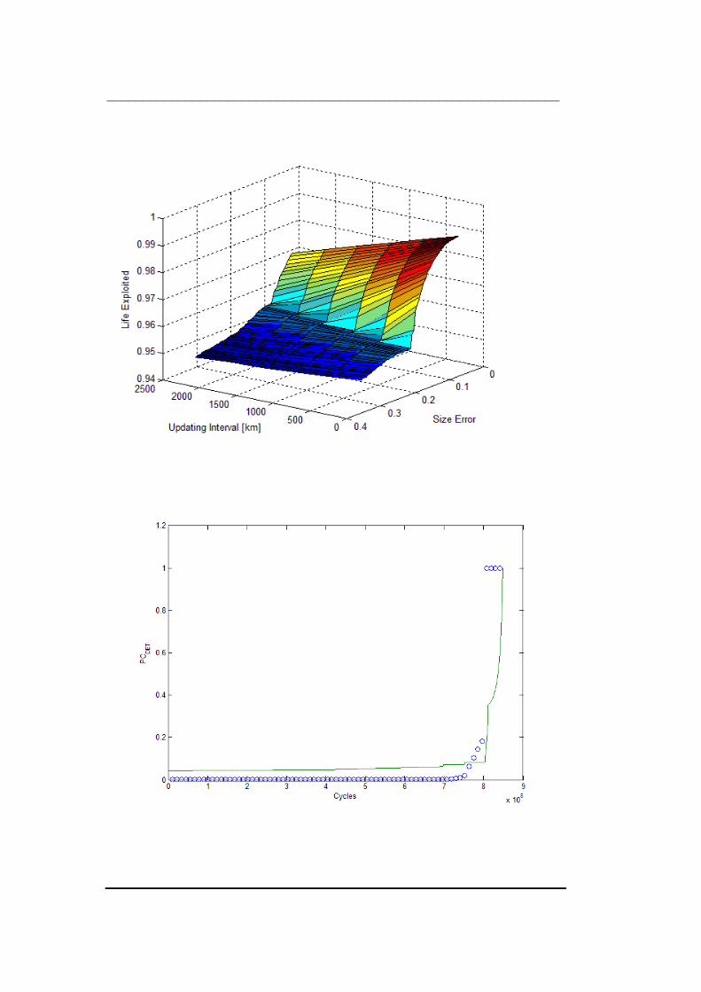
________________________________________________________________

________________________________________________________________
201
C7

________________________________________________________________

________________________________________________________________
203
C8

________________________________________________________________

________________________________________________________________
205

________________________________________________________________
C9

________________________________________________________________
207

________________________________________________________________
C10
m

________________________________________________________________
209