an improved scattering routine for collimation tracking studies at lhc
TRANSCRIPT
CER
N-T
HES
IS-2
014-
014
21/0
1/20
14
An improved scattering routine for collimationtracking studies at LHC
Facoltà di Scienze Matematiche, Fisiche e Naturali
Corso di Laurea Magistrale in Fisica
Candidate
Claudia TambascoID number 1218021
Thesis Advisor
Dr. Gianluca Cavoto
Co-Advisors
Dr. Stefano RedaelliDr. Maria Belen Salvachua Ferrando
Academic Year 2012/2013

An improved scattering routine for collimation tracking studies at LHCMaster thesis. Sapienza – University of Rome
© 2013 Claudia Tambasco. All rights reserved
This thesis has been typeset by LATEX and the Sapthesis class.
Author’s email: [email protected]

Dedicato a tutta la mia famiglia, per l’amore che mi ha sempre dimostrato.


v
Acknowledgments
The first person that I want to express my gratitude is my supervisor at CERNBelen Salvachua, with patience and devotion she guided me through this difficultpath. Never losing the smile, she has always helped me during the work,encouraged me and reassured me when difficult moments came. This work waspossible also because I learned a lot from her. Furthermore, I warmly thankBelen, not only for her concrete contribution to this thesis work, but also foralways having believe in me and in my capabilities.A Special thanks to the leader of LHC Collimation project Stefano Redaellithat gave me the possibility to work on this thesis project. He opened me newperspectives and gave me the chance to be part of an important work group.His precious experience was crucial to carry out this work. Working side byside with him enriched strongly both my professional and human experience.Thanks also to my home university supervisor Gianluca Cavoto, who acceptedto follow me in this experience. He has been a constant and reliable referencepoint on which I could always count.I wish to address a great thanks to the whole Collimation group and in particularto my colleagues that always helped me to solve any kind of problems: Danielethat was the first to explain to me the scattering routine code and he alwayshelped me by answering my many questions, Luisella that was always a preciousand friendly adviser, Roderik that concretely helped me in the last part of thework, Aurelien that helped me with his precious tricks on python scripts.And now I want to remember my family and Italian friends.Ringrazio tutta la mia famiglia: é grazie ai loro sacrifici che ho raggiuntoquesto importante obiettivo. Con infinito amore hanno sempre desiderato ilmeglio per me e lavorato sodo affinché potessi ottenerlo; per questo dedico aloro il mio lavoro di tesi, sperando di ripagarli, almeno in parte, per tuttoquello che hanno sempre fatto per me. Vi voglio tantissimo bene.Un ringraziamento speciale va a Vincenzo per essere stato accanto a me in ognimomento. Per avermi sostenuto nei momenti di difficoltá, e per avermi semprespronata a dare il meglio. Per aver avuto sempre pronto un buon consiglio, peravermi regalato tanti momenti di felicitá cancellando le mie paure, e per aversempre creduto in me e nel mio lavoro.Ringrazio Romina perché lei c’é sempre e perché durante tutti questi anni hasempre accettato e sopportato da buona amica le mie assenze a causa dellostudio. Per tutti i bei momenti passati insieme fin dal liceo e per essere semprepronta ad aiutarmi nel momento del bisogno. Ringrazio Maurilia e Manlio,buoni amici da tanto tempo.Ringrazio Elena, preziosa compagna di avventure qui a Ginevra nonché fedeleamica e consigliera.Ringrazio tutti i miei amici d’infanzia con i quali ho condiviso e continuo acondividere bei momenti di spensieratezza.

vi
Un caloroso ringraziamento va a tutti i mie colleghi dell’universitá con i qualiho affrontato difficili esami, periodi di studio intenso, interminabili tesine dilaboratorio e chi piú ne ha piú ne metta. In ogni caso, la loro compagnia hasempre reso tutto meno faticoso. Un caloroso grazie a Federica, Francesca,Elena, Ambra, Arianna, Maddalena, Matteo, Maddalena, Daniele, Andrea eValentina.Un sentito grazie a tutti gli amici che ho conosciuto a Ginevra, a Davidone e aRobertone che spero d’ incontrare di nuovo al piú presto ed a Valentina.Infine voglio dire grazie, perché no, anche a me stessa. Per tutta la volontá cheho avuto in questi anni di studio, per tutti gli sforzi che ho fatto per arrivarefin qui e per non essermi arresa mai.

vii
Contents
1 Introduction 7
2 Collimation theory for circular accelerators 92.1 Basic concepts of linear beam dynamics . . . . . . . . . . . . . . . . 9
2.1.1 Transverse motion and betatron oscillations . . . . . . . . . . 102.1.2 Dispersion . . . . . . . . . . . . . . . . . . . . . . . . . . . . . 142.1.3 Longitudinal motion: synchrotron oscillations . . . . . . . . . 15
2.2 Collimation system . . . . . . . . . . . . . . . . . . . . . . . . . . . . 182.2.1 Machine aperture and beam acceptance . . . . . . . . . . . . 182.2.2 Beam halo population . . . . . . . . . . . . . . . . . . . . . . 182.2.3 Collimation procedure . . . . . . . . . . . . . . . . . . . . . . 202.2.4 Cleaning performance . . . . . . . . . . . . . . . . . . . . . . 212.2.5 Maximum beam intensity from cleaning inefficiency . . . . . 22
3 The Large Hadron Collider 233.1 The accelerator complex . . . . . . . . . . . . . . . . . . . . . . . . . 243.2 The LHC collimation . . . . . . . . . . . . . . . . . . . . . . . . . . . 25
3.2.1 LHC collimator design . . . . . . . . . . . . . . . . . . . . . . 263.2.2 The multi-stage collimation system at LHC . . . . . . . . . . 283.2.3 Collimator layout for beam cleaning and experiments protection 29
4 Collimation cleaning setup 334.1 SixTrack for collimation . . . . . . . . . . . . . . . . . . . . . . . . . 334.2 Particle Tracking . . . . . . . . . . . . . . . . . . . . . . . . . . . . . 334.3 Input files to run SixTrack . . . . . . . . . . . . . . . . . . . . . . . . 34
4.3.1 Machine lattice . . . . . . . . . . . . . . . . . . . . . . . . . . 354.3.2 Collimator properties . . . . . . . . . . . . . . . . . . . . . . 354.3.3 SixTrack setting file . . . . . . . . . . . . . . . . . . . . . . . 36
4.4 Post processing and simulation outputs . . . . . . . . . . . . . . . . 374.5 SixTrack reference plots for collimation studies . . . . . . . . . . . . 39
4.5.1 Collimator setting and layout . . . . . . . . . . . . . . . . . . 404.5.2 Distribution of the generated beam halo . . . . . . . . . . . 404.5.3 Distribution of impacts at primary collimators . . . . . . . . 414.5.4 Distribution of impacts at TCTs and dump protection . . . . 434.5.5 Particle lost at aperture in the Dispersion Suppression region
at IR7 . . . . . . . . . . . . . . . . . . . . . . . . . . . . . . . 44

viii Contents
4.5.6 Standard loss maps and cleaning efficiency . . . . . . . . . . . 44
5 Improved physics model for SixTrack scattering routine 475.1 SixTrack scattering routine . . . . . . . . . . . . . . . . . . . . . . . 485.2 Electromagnetic processes . . . . . . . . . . . . . . . . . . . . . . . . 50
5.2.1 Ionization . . . . . . . . . . . . . . . . . . . . . . . . . . . . . 505.2.2 Multiple Coulomb Scattering . . . . . . . . . . . . . . . . . . 51
5.3 Nuclear Interactions . . . . . . . . . . . . . . . . . . . . . . . . . . . 535.3.1 Proton-nucleon nuclear scattering . . . . . . . . . . . . . . . . 565.3.2 Proton-nucleus scattering . . . . . . . . . . . . . . . . . . . . 615.3.3 Rutherford scattering . . . . . . . . . . . . . . . . . . . . . . 63
5.4 Material properties . . . . . . . . . . . . . . . . . . . . . . . . . . . . 635.5 Detailed distribution of individual processes . . . . . . . . . . . . . . 64
6 Validation of the improved scattering routine of SixTrack 676.1 Effect of scattering routine updates on simulations . . . . . . . . . . 67
6.1.1 Simulation setup . . . . . . . . . . . . . . . . . . . . . . . . . 686.1.2 Cleaning inefficiency . . . . . . . . . . . . . . . . . . . . . . . 696.1.3 Impacts at collimators . . . . . . . . . . . . . . . . . . . . . . 69
6.2 Measurements of beam losses at the LHC . . . . . . . . . . . . . . . 706.2.1 Generation of beam losses: ADT and resonance method . . . 706.2.2 The BLM system . . . . . . . . . . . . . . . . . . . . . . . . . 716.2.3 Loss maps during LHC Run I (2010-2013) . . . . . . . . . . . 71
6.3 Validation of the SixTrack scattering routine with data . . . . . . . . 716.3.1 Machine configuration . . . . . . . . . . . . . . . . . . . . . . 726.3.2 Collimator settings . . . . . . . . . . . . . . . . . . . . . . . . 726.3.3 BLM response factor . . . . . . . . . . . . . . . . . . . . . . . 736.3.4 Comparisons between data and simulations . . . . . . . . . . 75
7 Improved estimation for 7TeV cleaning performance 797.1 Machine configuration at 7TeV . . . . . . . . . . . . . . . . . . . . . 797.2 Loss maps at 7TeV . . . . . . . . . . . . . . . . . . . . . . . . . . . . 817.3 Impacts at the primary collimators . . . . . . . . . . . . . . . . . . . 857.4 Losses at Dispersion Suppressor region at IR7 . . . . . . . . . . . . . 867.5 Impacts on TCTs . . . . . . . . . . . . . . . . . . . . . . . . . . . . . 887.6 Parametric study for 7TeV simulations . . . . . . . . . . . . . . . . . 89
8 Conclusions 93
Bibliography 99

1
List of Figures
2.1 Coordinate system respect to the beam direction . . . . . . . . . . . 102.2 Particle trajectory in the phase space. . . . . . . . . . . . . . . . . . 122.3 Trajectory in the x− x′ phase space . . . . . . . . . . . . . . . . . . 152.4 Example of energy gain in the RF potential . . . . . . . . . . . . . . 162.5 Motion in the phase space . . . . . . . . . . . . . . . . . . . . . . . . 172.6 Trajectory of the synchrotron oscillations in the phase space. . . . . 172.7 Geometrical and dynamic apertures in an accelerator . . . . . . . . . 192.8 Collimator jaws along beam path . . . . . . . . . . . . . . . . . . . . 202.9 Two-stage collimation system. . . . . . . . . . . . . . . . . . . . . . . 21
3.1 Layout of the LHC . . . . . . . . . . . . . . . . . . . . . . . . . . . . 233.2 Accelerator complex at CERN . . . . . . . . . . . . . . . . . . . . . 253.3 Scheme of LHC collimator . . . . . . . . . . . . . . . . . . . . . . . . 273.4 Top collimator view . . . . . . . . . . . . . . . . . . . . . . . . . . . 283.5 Schematic layout of the LHC multi-stage collimation system . . . . . 293.6 General collimators layout and cleaning insertions of LHC . . . . . . 30
4.1 The thin lens formalism . . . . . . . . . . . . . . . . . . . . . . . . . 344.2 Fragment of the fort.2 file . . . . . . . . . . . . . . . . . . . . . . . . 354.3 Fragment of the collimator database file . . . . . . . . . . . . . . . . 374.4 Halo distribution in the phase space . . . . . . . . . . . . . . . . . . 374.5 Extract from the fort.3 input file . . . . . . . . . . . . . . . . . . . . 384.6 Example of a trajectory of a particle lost in the LHC aperture . . . . 394.7 Summary list of reference plots with the SixTrack output files . . . . 394.8 Collimator setting with the half-gap in σ units for the 7TeV case. . . 404.9 Collimator layout for Beam 1 4TeV. . . . . . . . . . . . . . . . . . . 404.10 Particle distribution in different spaces . . . . . . . . . . . . . . . . . 414.11 Transverse distribution of the first impacts on the primary collimators. 424.13 All impacts plots. . . . . . . . . . . . . . . . . . . . . . . . . . . . . . 424.14 Number of absorbed particles at different IP collimators . . . . . . . 434.15 Distribution of the particle lost in the aperture of the DS region in IR7. 444.16 Simulated beam loss map at 7TeV for Beam 1 in the horizontal plane 45
5.1 Scheme of the calls between different subroutines in SixTrack scatter-ing routine. . . . . . . . . . . . . . . . . . . . . . . . . . . . . . . . . 48
5.2 Representation of particle position close to collimator jaw. . . . . . . 495.3 Implemented Bethe-Bloch formula . . . . . . . . . . . . . . . . . . . 50

2 List of Figures
5.4 Schematic view of MCS in one plane . . . . . . . . . . . . . . . . . . 525.5 Multiple Coulomb scattering angle (rms) in the (s − x) plane for
different path with the collimator jaw. . . . . . . . . . . . . . . . . . 545.6 Distribution in x′ of the particles at the end of the horizontal primary
collimator . . . . . . . . . . . . . . . . . . . . . . . . . . . . . . . . . 555.7 Distribution of the mean free path (λ) . . . . . . . . . . . . . . . . . 565.8 Elastic, inelastic and total cross sections from TOTEM Collaboration 575.9 The slope parameter for pp and pp elastic scattering. . . . . . . . . . 585.10 Total pp and pp single diffractive cross section . . . . . . . . . . . . . 595.11 Triple-pomeron Feynman diagram for single diffraction . . . . . . . . 595.13 Experimental measurements of the slope factor parameter for proton-
nucleus elastic scattering . . . . . . . . . . . . . . . . . . . . . . . . . 615.14 Angular distribution of the proton-proton single diffractive scattering 645.15 Angular distribution of the proton-proton elastic scattering . . . . . 655.16 Angular distribution of the proton-nucleus elastic scattering . . . . . 655.17 Energy variation of the scattered proton after p-p single diffractive
process. . . . . . . . . . . . . . . . . . . . . . . . . . . . . . . . . . . 65
6.1 Collimator settings for Beam 1 at 7 TeV . . . . . . . . . . . . . . . . 686.2 Beta function at IP5 and IP2 for Beam 1 7 TeV . . . . . . . . . . . . 686.3 Cleaning inefficiency for simulations at 7TeV in the IR7 cold magnets 696.4 Particles absorbed at all collimators normalized to the particles ab-
sorbed at the horizontal primary collimator in IR7. . . . . . . . . . . 706.5 Collimation cleaning inefficiency as function of time since 2010 until
end of 2012 run . . . . . . . . . . . . . . . . . . . . . . . . . . . . . . 716.6 Distribution of the losses in the LHC ring . . . . . . . . . . . . . . . 726.7 Distribution of the losses in the betatron cleaning insertion IR7 . . . 726.8 Beta-star at IP5 for protons at 3.5 TeV . . . . . . . . . . . . . . . . . 736.9 Beta-star at IP2 and IP8 for protons at 3.5 TeV . . . . . . . . . . . . 736.11 Losses at 3.5TeV from experimental data compared with the simula-
tions performed with the new and old SixTrack version. . . . . . . . 766.12 Simulated loss map at 3.5TeV. . . . . . . . . . . . . . . . . . . . . . 776.13 BLM signal ratio on horizontal and vertical TCTs to the TCPs in
simulations and measurements in the 2011 machine . . . . . . . . . . 78
7.4 Simulated beam loss map at 7TeV with the new routine for Beam 1horizontal halo case. . . . . . . . . . . . . . . . . . . . . . . . . . . . 81
7.5 Simulated beam loss map at 7TeV with the new routine for Beam 1vertical halo case. . . . . . . . . . . . . . . . . . . . . . . . . . . . . . 82
7.6 Simulated beam loss map at 7TeV with the new routine for Beam 2horizontal halo case. . . . . . . . . . . . . . . . . . . . . . . . . . . . 83
7.7 Simulated beam loss map at 7TeV with the new routine for Beam 2vertical halo case. . . . . . . . . . . . . . . . . . . . . . . . . . . . . . 84
7.13 Total of particle lost in the DS region at IR7 for Beam 1 horizontalhalo case. . . . . . . . . . . . . . . . . . . . . . . . . . . . . . . . . . 87
7.14 Number of particles absorbed in TCT collimators with new scatteringroutine and the previous one . . . . . . . . . . . . . . . . . . . . . . 89

List of Figures 3
7.15 Effects on the impacts at TCT collimators in IR1 and IR5 for aσSDpp ± 20% variation and a σSDpp ± 50% variation, Beam 1 with ahorizontal halo distribution. . . . . . . . . . . . . . . . . . . . . . . 91


5
List of Tables
3.1 LHC main design parameters . . . . . . . . . . . . . . . . . . . . . . 263.2 Material jaws for different collimator types. . . . . . . . . . . . . . . 273.3 Collimator settings for the different families in the cleaning hierarchy 31
4.1 Collimator materials and densities implemented in SixTrack. . . . . 36
5.1 Loss energy rate for Eref = 450GeV previously tabulated in SixTrackand values with the new Bethe-Bloch function at E = 7TeV . . . . . 51
5.2 Total single diffractive cross section for previous and new SixTrack . 605.3 Total proton-proton cross sections from the previous SixTrack imple-
mentation and the updated one. . . . . . . . . . . . . . . . . . . . . 605.4 Atomic mass, nuclear interaction length and reference inelastic cross
section . . . . . . . . . . . . . . . . . . . . . . . . . . . . . . . . . . . 625.5 Atomic mass, nuclear collision length and reference total proton-
nucleus cross sections . . . . . . . . . . . . . . . . . . . . . . . . . . . 635.6 Nuclear and atomic properties for implemented materials in SixTrack 64
6.1 Collimator settings during 2011 Run with protons at 3.5 TeV beamenergy . . . . . . . . . . . . . . . . . . . . . . . . . . . . . . . . . . . 74
6.2 BLM response factors from FLUKA and SixTrack for Beam 1 hori-zontal halo . . . . . . . . . . . . . . . . . . . . . . . . . . . . . . . . 74
6.3 BLM response factors from FLUKA and SixTrack for Beam 1 verticalhalo . . . . . . . . . . . . . . . . . . . . . . . . . . . . . . . . . . . . 75
6.4 Maximum of losses on the cold magnets for the simulations with thenew SixTrack version and the old SixTrack version . . . . . . . . . . 75
6.5 Integrated losses on the cold magnets for simulations with the newSixTrack version and the old SixTrack version . . . . . . . . . . . . . 75
7.2 Beam losses and the ratio in the dispersion suppressor at IR7 Beam 1horizontal halo. . . . . . . . . . . . . . . . . . . . . . . . . . . . . . . 88
7.3 Beam losses and the ratio in the dispersion suppressor at IR7 Beam 1vertical halo. . . . . . . . . . . . . . . . . . . . . . . . . . . . . . . . 88
7.4 Beam losses and the ratio in the dispersion suppressor at IR7 Beam 2horizontal halo. . . . . . . . . . . . . . . . . . . . . . . . . . . . . . . 88
7.5 Beam losses and the ratio in the dispersion suppressor at IR7 Beam 2vertical halo. . . . . . . . . . . . . . . . . . . . . . . . . . . . . . . . 88

6 List of Tables
7.6 Maximum cleaning inefficiency on the cold magnets in IR7 for ± 20%variation of single diffractive cross section. . . . . . . . . . . . . . . . 90
7.7 Maximum cleaning inefficiency on the cold magnets in IR7 for ± 50%variation of single diffractive cross section. . . . . . . . . . . . . . . . 90
7.8 Maximum cleaning inefficiency on the cold magnets in IR7 for ± 20%variation of proton-proton elastic cross section. . . . . . . . . . . . . 90
7
Chapter 1
Introduction
The first particle accelerator was built in the 1920s to investigate the structure ofthe atomic nucleus. Since then, more and more energetic particle accelerators havebeen designed to investigate many other aspects of particle physics.The Large Hadron Collider is the world’s largest and highest energy particle accel-erator ever built. It was commissioned by the European Organization for NuclearResearch (CERN) in collaboration with more than 10000 scientists and engineersfrom over 100 countries and hundreds of universities and laboratories. The construc-tion of the LHC started in 1999. The LHC accelerates proton and ion beams up to7TeV and 574 TeV respectively. The protons circulated for the first time the entirering of the LHC on 10th September 2008, with an energy less than 1TeV. The twocounterrotating beams collide in the experiment detectors installed in four points onthe accelerator ring. The two beams are accelerated by the electric field of the Ra-diofrequency (RF) cavities shaped to resonate at specific frequencies, allowing radiowaves to interact with the passing particles. To bend and focus the circulating beamssuperconducting magnets (SC) are located around the beam pipes. They work atvery low temperature, between 1.8K and 4.5K, if for some reasons the temperatureof the magnets increases the SC magnets can lose their superconducting state andquench. The heating of the SC magnets can be caused by the energy depositioninduced by local beam losses. Beam losses of 4·107 protons at 7TeV correspond toan energy deposition of 30 mJ cm3. To prevent beam losses, which are dangerousfor the machine components, an efficient collimation system is of crucial importance.The LHC is equipped with a multi-stage collimation system that provides beamcleaning and passive machine protection. The beam core particles perform a stablemotion around the ring while the particles that populate the so-called "beam halo",at the tails of the beam, will be uncontrollably lost in the machine. A collimatorconsist of two fully movable parallel jaws installed along the beam pipe. The twojaws are positioned at a specific distance creating a gap within which the particles ofthe beam core can pass unperturbed. The halo particles are intercepted and cleanedby the collimator jaws material, reducing considerably the risk of uncontrolled beamlosses.At the LHC different types of beam cleaning are provided by the collimation system:in the insertion IR3, is installed the collimation system that provides the cleaning ofthe off-momentum particles, while in the insertion IR7 particles with too large trans-

8 1. Introduction
verse oscillation amplitudes are intercepted by the collimators providing betatroncleaning. In addition to protect the machine by radiation damage, the beam cleaningminimize the background for the LHC experiments. The cleaning performance of thecollimation system is expressed by the cleaning efficiency. This parameter expressesthe fraction of particles that hit a primary collimator and are stopped in the cleaninginsertion. A cleaning efficiency above 99.99% must be reached to optimize the LHCperformance.The present work aims to increase the prediction power of the collimation per-formance at 7TeV energy. Collimation studies for the LHC are performed withSixTrack, a dedicated simulation tool that tracks a large numbers of particles formany turns around the ring. The SixTrack code includes a scattering routine tomodel proton interactions with the collimators jaws. During the thesis work the scat-tering routine has been updated taking into account recent experimental data. Theimplemented updates allow an improved modeling capability for the 7TeV protonbeam interactions and to extract a better estimation of the cleaning performance ofthe collimation system. The results will be provided as input for collimation studiesat higher energy.The first part of the thesis introduces some useful fundamental concepts to analyzethe present work. In particular in Chapter 2 the basic principles of linear beamdynamics, focusing on transversal and longitudinal motion, are covered together withsome collimation theory concepts. The third chapter provides a brief introductionto the LHC detailing its collimation system. The main parameter for SixTrack codesetup and the reference plots for collimation studies are presented in Chapter 4.The physics model of the scattering routine is described in detail in Chapter 5, eachcross section characterizing the interaction between the proton and the materialnuclei of the collimator jaw is taken into account. For each process the basic theoryis introduced, followed by the description of the updates implemented accordingto recent available data. In order to asses the improvement with respect to theprevious scattering routine version a comparison with the data is carried out. Thelast chapter is dedicated to the 7TeV cleaning performance study with the newSixTrack version. In particular beam losses in the most critical machine region, thedispersion suppressor region are presented with the complete loss distribution aroundthe ring. A parametric study of the effects on the collimation cleaning caused bythe uncertainty of the proton-proton single diffractive cross section is also reported.This study can be a useful reference for future collimation studies at higher energy.

9
Chapter 2
Collimation theory for circularaccelerators
The beams of a circular accelerator can be represented as bunches of particles forwhich the distribution inside each bunch can be considered as a Gaussian. Thecentre of the Gaussian distribution represents the particles that are the core of thebunch and perform stable oscillations along the designed orbit. Several processescan kick these particles and deviate them from the nominal orbit of the accelerator,populating thus the primary halo represented by the tails of the Gaussian. The haloparticles perform unstable motion and can be lost at the aperture of the machinewith the consequent release of energy that can damage the superconducting magnets.In order to avoid large energy depositions in the cold magnets an efficient collimationsystem in needed. The collimators intercept the particles that populate the tails ofthe particle distribution providing halo cleaning and protecting the machine.
2.1 Basic concepts of linear beam dynamics
The motion of particles inside the ring is driven by electric and magnetic fields.The electric field accelerates the particles and compensates the energy lost bysynchrotron radiation. This field is generated by the Radiofrequency cavities (RF)that are resonant cavities with an applied sinusoidal potential difference synchronizedwith the particles of nominal momentum. The RF provide the energy for acceleratingthe particles and defines a spatial region called RF bucket that contains the particlessynchronous with the RF. The particles outside the bucket will be loosing energyturn by turn until they are lost ideally at the collimators. The beam particles moveinside the buckets grouped in bunches. The magnetic fields of several orders, dipole,quadrupoles, sextuples, octupoles and so on, define the motion of the particlesthrough the machine. In particular, the dipole magnets determine a close orbit bybending the charged particles. Ideally, a particle with nominal energy can moveinfinitely along the closed orbit of the machine. However, in a non-ideal world, theparticle is diverging from the nominal orbit and needs a focus strength to keep thenominal orbit. The quadrupoles focus the beam acting as an optical lens. Theeffect of the electric and the magnetic field on a charged particle is described by the

10 2. Collimation theory for circular accelerators
Figure 2.1. Coordinate system respect to the beam direction [1].
Lorentz force:d~p
dt= q( ~E + ~v ∧ ~B), (2.1)
where ~p is the relativistic momentum of the particle, ~v is the velocity, q the chargeand ~E and ~B the electric and the magnetic fields respectively. On the one handthis formula illustrates how a magnetic field will generate a change of momentumperpendicular to the velocity of the particle, thus being able to act in the trajectoryof the particle and bend it. On the other hand an electric field will provide a changeof momentum in the same direction of the field which could be used to accelerate ordecelerate particles. In the following sections the longitudinal and the transversemotion of the particles along the ring will be described in more details.
2.1.1 Transverse motion and betatron oscillations
In this section we describe the transverse motion of a particle in an accelerator ringconsidering the steady state of the machine, that is not during the phase of injection,acceleration or extraction of the beams [1, 2, 3]. The reference system is representedin Fig.2.1, it is a right-handed orthogonal and moving system (x, y, s) and it takesthe name of Frenet-Serret. The charged particle moves on the circular blue line,that represents the ideal closed orbit where ~r0 is the orbital radius. The vectors ~s, ~xand ~y are respectively the tangential, horizontal and vertical position of the particlerelative to the orbit.A charged particle of momentum p is guided by dipoles that force the particle tocurve and to follow circular orbit. By equating the centrifugal force and the Lorentzforce:
F = qvB = γmv2
ρ, (2.2)
where B is a constant field perpendicular to the particle velocity, the local radius(ρ) is given by:
ρ = p
qB(2.3)
The magnetic rigidity R is defined as:
R = Bρ = p
q. (2.4)

2.1 Basic concepts of linear beam dynamics 11
and it directly relates the effect of the magnetic field on the motion of chargedparticles.The equation of motion can be derived using a linear approximation by consideringthat there is no longitudinal homogeneous component of the magnetic field, i.e~B = (Bx, By, 0). The transverse components may be expanded in Taylor series tothe first order [1] for small deviation from the designed orbit:
Bx(x, y, s) = Bx0 + ∂Bx∂x
x+ ∂Bx∂y
y (2.5)
By(x, y, s) = By0 + ∂By∂x
x+ ∂By∂y
y. (2.6)
From the Maxwell’s equations we know the following relations:
∂Bx∂x
= −∂By∂y
,
∂By∂x
= ∂Bx∂y
.
(2.7)
We assume that the magnetic field is constant just on the vertical plane and zero inthe horizontal plane, so the particle is bent on the horizontal plane. This means:Bx0 = 0 and ∂By
∂y = 0. By assuming no skew quadrupolar fields (∂Bx∂x = 0) the Eq. 2.5
and Eq. 2.6 can be written:Bx = ∂By
∂xy = B1y, (2.8)
By = −B0 + ∂By∂x
x = −B0 +B1x, (2.9)
where B0 and B1 are the coefficients of dipole and quadrupole respectively. Consid-ering only particles of designed momentum and keeping only the linear terms, theso-called Hill’s equations that describe the transverse motion are given [1]:
x′′ +Kx(s)x = 0, Kx(s) = 1ρ(s)2 −
B1(s)Bρ(s) (2.10)
y′′ −Ky(s)y = 0, Ky(s) = −B1(s)Bρ(s) (2.11)
with x′ = dx/ds and x′′ = d2x/ds2. Assuming the magnetic terms ρ(s) andKy(s) areconstant in s inside a magnetic element, the Eq. 2.10 and Eq. 2.11 give respectivelythe solutions of an harmonic oscillator or an exponential function, depending on thesign Ky. The solution of the Hill’s equations, in the x direction is [2]:
x(s) = A√βx(s) sin(ϕx(s) + ϕ0) (2.12)
where βx(s) is the betatron function that is a periodic function and modulates theamplitude A of the betatron oscillations in the transversal plane, ϕ0 is an constantphase. The solution for the y coordinate get the same form of Eq.2.12. The phaseadvance is ϕx(s) and is given by:
ϕ(s) =∫ s
0
ds′
β(s′) . (2.13)

12 2. Collimation theory for circular accelerators
Figure 2.2. Particle trajectory in the phase space.
Each particle is characterized by different values of the constant A and its squareroot is known as single-particle emittance εx. The Eq. 2.12 can be rewritten as:
x(s) =√εxβx(s) sin(ϕx(s) + ϕ0). (2.14)
Therefore, the motion in the transversal plane of the travelling particles aroundthe accelerator ring is a sine-like trajectory with a varying amplitude εx
√βx(s)
modulated by the betatron function and with a phase ϕx(s) + ϕ0 that advanceswith s at vayring rate proportional to 1/β. In the phase space (x, x′), the particlemoves on an elliptical trajectory (Fig.2.2). The particle trajectory is described bythe following equation [3]:
εx = γx(s)x2(s) + 2αx(s)x(s)x′(s) + βx(s)x′2(s) (2.15)
where:αx(s) = −β
′x(s)2 (2.16)
γx(s) = 1 + α2x(s)
βx(s) (2.17)
α(s), β(s) and γ(s) are called Twiss parameters [3] and completely define themachine optics.The shape of the ellipse depends on the s position in the machine, while the areadoes not change if the particles have a constant energy and stochastic effects areneglected during the motion. In the transversal phase space, all the particles ofthe beam can be represented by a Gaussian distribution of points with a σx calledbetatronic beam size and divergence σ′x(s):
σx =√εrmsx βx(s) (2.18)

2.1 Basic concepts of linear beam dynamics 13
σ′x =√εrmsx γx(s) (2.19)
where εrmsx is the root mean square emittance and is defined as:
εrmsx =
√< x2 >< x′ 2 > − < xx′ >2. (2.20)
The beam core is defined as the group of particles within 3σ(s) from the centre ofthe beam, while the tail or beam halo are all the particles outside that range. It ispossible to define a normalized εx emittance, that does not vary with the particleenergy, as following:
εnormx = γβrelε
rmsx (2.21)
with βrel = vc , v is the particle velocity, c is the speed of light in the vacuum and
γ = 1√1−β2
rel
.An important parameter for describing the transversal motion, is the tune that isthe number of betratron oscillations, i.e. the number of turns in the phase space, inone machine revolution. It is defined as:
T = 12πϕ(C) = 1
2π
∫ s0+C
s0
ds
β(s) . (2.22)
The tune is chosen to be an irrational number and it guarantees that the orbit in thephase space is dense. It means that the particle will pass through all the acceleratorlocated at the sigma of its orbit. This irrationality also avoids resonances that canyield the machine to be unstable leading the loss of the beam.If a particle is at a certain point s1 of the machine, is possible to predict the evolutionof the phase space coordinates by using the transport matrix. This matrix allows tocalculate x and x′ from the point s1 to a downstream location s2. The Eq. 2.12 canbe rewritten in the following way:
x(s) = a√β(s) sin(ϕ(s)) + b
√β(s) cos(ϕ(s)) (2.23)
where a and b are functions of x and x′:
a = x(s1)[[ sin(ϕ(s1)) + α(s1) cos(ϕ(s1))√
β(s1)
]+ x′(s1)
√β(s1) cos(ϕ(s1)) (2.24)
b = x(s1)[[ cos(ϕ(s1))− α(s1) sin(ϕ(s1))√
β(s1)
]− x′(s1)
√β(s1) sin(ϕ(s1)) (2.25)
By substituting Eq. 2.24 and Eq. 2.25 in the Eq. 2.23 is possible to obtain the solutionfor x(s2) and x′(s2) in a matricial form:(
x(s2)x′(s2)
)= M(s1|s2)
(x(s1)x′(s1)
)(2.26)
where:
M(s1|s2) =
√
β1β2
(cosϕ21 + α1 sinϕ21)√β1β2 sinϕ21
−1+α1α2√β1β2
sinϕ21 + α1−α2√β1β2
cosϕ21√
β1β2
(cosϕ21 − α2 sinϕ21
(2.27)

14 2. Collimation theory for circular accelerators
where ϕ21 is the phase advance and the matrix M(s2|s1) is the transport matrix.For on-momentum particles with reference momentum p0, is possible to use thetransport matrix to calculate the phase space coordinates x and x′ in any points ofthe accelerator. In the normalized space, the previous formula takes the followingsimplified form:
M(s1|s2) =(
cosϕ21 sinϕ21− sinϕ21 cosϕ21
)(2.28)
that is a classical rotation matrix.
2.1.2 Dispersion
In the transverse plane, the effect of a momentum offset causes the distortion of theclose orbit around which the particles perform betatron oscillations. The momentumvariation is defined as:
δ = p− p0p0
(2.29)
for small momentum variations the Eq.2.10 becomes:
x′′ +K(s)x = δ
ρ(s) (2.30)
The solution of the previous equation is:
x(s) = xβ(s) + xδ(s) (2.31)
where xβ is the betatron oscillation around the on-momentum orbit and xδ is theparticular solution of the inhomgeneous equation (2.30) and gives the shift due tothe energy variation. It can be also expressed as follow:
xδ = D(s)δ (2.32)
where D(s) is the dispersion function that satisfies the equation:
D′′ +K(s)D = 1ρ(s) (2.33)
The shift for x′(s) can be expressed as above:
x′δ(s) = D′(s)δ (2.34)
and then the total solution for the angle is:
x′(s) = x′β(s) + x′δ(s) (2.35)
a similar argument can be made for the solution in y. The dispersion effect leads toa shift of the ellipse center in the phase space as is shown in Fig.2.3
2.1 Basic concepts of linear beam dynamics 15
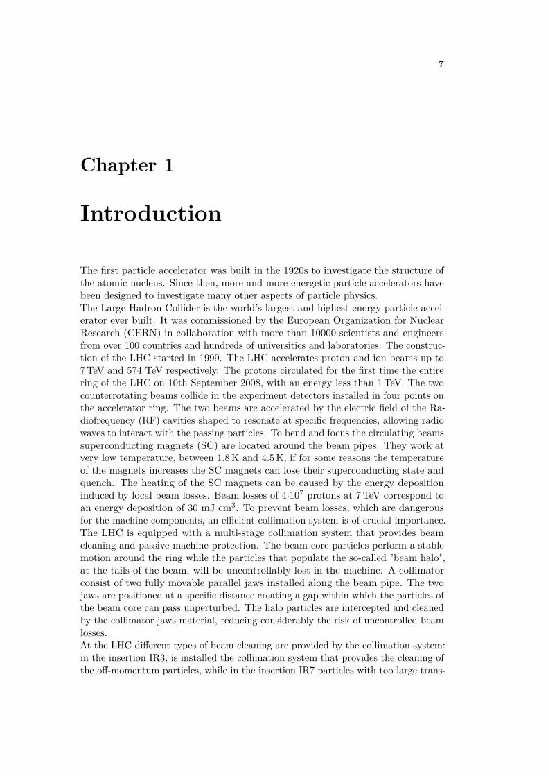
Figure 2.3. Trajectory in the x− x′ phase space for a particle with momentum offset δ.
2.1.3 Longitudinal motion: synchrotron oscillations
The longitudinal electric field in the RF cavities accelerates the charged particlesin the beam. The RF cavities consist of isolate gaps with a sinusoidal voltageapplied. When the beam passes through the RF, the particles are accelerated ordecelerated depending on the synchronized arrival inside the RF. In order to setthe particles inside the accelerating region of the RF period the beam is split inseveral bunches, the frequency ωRF of the electric field is an integer multiple of therevolution frequency in the ring:
ωRF = hωREV (2.36)
where h is called the harmonic number. The energy gain of the particles at eachpassage in the cavity is:
∆E = qV0 sinϕ(t) (2.37)
where q is the charge of the particle, V0 is the amplitude of the potential of the cavityand ϕ is the phase of the particle with respect to the RF phase. The circulatingparticles lose energy, in part due to synchrotron radiation, this energy variationchanges the length L of the orbit as follows:
∆LL
= αc∆pp
(2.38)
in which αc is a factor called momentum compaction factor [2] and depends only onthe bending radius of the particle orbit and the dispersion. Ideally, the referenceparticle that is synchronous with the RF, arrives always with the same relativephase ϕs. The other particles of the bunch arrive earlier or later and gain differentamounts of energy by passing across the RF cavity. Supposing that the particle

16 2. Collimation theory for circular accelerators
Figure 2.4. Example of energy gain in the RF potential for particles (blue dots) close tothe synchronous one (red dots).
velocities are well below the speed of light, a particle B with less energy respect tothe synchronous particle, arrives late in the RF and receives an additional amountof energy (see Fig.2.4). In the next turn the energy of the particle B will be greaterand it will arrive earlier with respect to A in the RF, receiving a lower energygain. Therefore the particle B oscillates around the synchronous particle energyposition as an harmonic oscillator [3]. The motion in the phase-space diagram isrepresented by the ellipse showed in Fig.2.5. The phase focusing principle determinesthe longitudinal stability of the bunch:
∆TT
=(αc −
1γ2
) ∆pp
(2.39)
with T being the revolution period in the ring and γ = Emc2 the ralativistic gamma.
Two different regimes are defined:
1. γ <√
1αc, so-called below transition
2. γ >√
1αc, so-called above transition
where the term:√
1αc
is the transition energy. In the case 1, the bunch stabilityis ensured in the angular range 0 < ϕs < π/2 corresponding to the rising part ofthe energy gained showed in Fig.2.4. In this case more energetic protons reachthe RF earlier than the synchronous particle (ϕ(t) < ϕs) so they gain less energyand when they will pass through the RF in the next turn, they will get closer tothe synchronous proton. On the contrary, less energetic particles arrive late in theRF (ϕ(t) > ϕs) gaining more energy and approaching the reference proton in thefollowing turn. Above transition (case 2), due to the relativistic effect of the timedilatation, a particle with higher energy has a longer revolution time and reach theRF later (ϕ(t) > ϕs). Similay to the case 1, the stability condition is satisfied inthe angular range of π/2 < ϕs < π. The oscillations performed around the reference

2.1 Basic concepts of linear beam dynamics 17
Figure 2.5. Motion in the phase space for a particle (B) that performs oscillations aroundthe synchronous particle (A).
Figure 2.6. Trajectory of the synchrotron oscillations in the phase space.
particle are called synchrotron oscillations. For particles with small longitudinalamplitude, the synchrotron oscillations describe a stable motion of equation:
ϕ+ Ω2s
cosϕs(sinϕ− cosϕs) = 0 (2.40)
where Ωs is constant. Because the Eq.2.40 is highly non-linear, there is an orbit ofstability called separatrix. Fig.2.6 represents the motion in the phase space withaction-angle variables. The stable particles oscillate on closed orbits within thearea delimited by the separatrix. This region of stability is called RF bucket. Theparticles that move on a trajectory beyond of it become unstable and will be lost inthe accelerator machine. The limit energy ∆Eb is defined by the following equation:
∆Eb = k
√1−
(π
2 − ϕs)
tanϕs, k = constant. (2.41)
This gives the energy acceptance of the accelerator machine. In the LHC for RFfrequency ωRF = 400MHz, the energy acceptance is ∆Eb = 3.53× 10⁻⁴δp/p at the

18 2. Collimation theory for circular accelerators
nominal energy of 7TeV.
2.2 Collimation systemDuring the motion in the accelerator machine, the particles undergo different effectsthat increase the beam emittance. As a result some particles slowly move towardsthe walls of the machine populating the beam tails and turn by turn they will belost. Other effects generate the beam halo that can be dangerous for the acceleratormachine. Collimation is needed to avoid background in high energy physics detector,to avoid quenching of the superconducting magnets and to limit the irradiation ofequipment in high intensities machine. The collimators are blocks of materials thatintercept the particles in the beam tails providing beam cleaning.
2.2.1 Machine aperture and beam acceptance
The vacuum chamber that with different elements installed along the full length (Lm)of the machine (beam screens, collimators, diagnostic equipments, etc.) constitutethe physical space where the particle beam moves called geometrical aperture Ageo.The aperture is commonly expressed in units of the standard deviation of the beamsize in a certain plane z = (x, y), which is defined as follows:
σz(s) =√βz(s)ε+ (Dz(s)δ)2 (2.42)
To ensure that at any location, all the particles are contained in the geometricaperture, it must be bigger than the maximum oscillation amplitude of the beamparticles. The maximum area of the phase space ellipse, i.e. the maximum emittance,that can be covered by a particle without being lost in the machine, is called beamacceptance Az. It is related to the geometrical aperture Ageo in the considered planez according to the formula:
Az(s) = (Ageo · σz(s))2
βz(s). (2.43)
A particle that hits the opening will be lost at that location, as soon as it satisfiesthe following condition:
Az ≥ Ageo · σz(s) (2.44)
Moreover in a real accelerator the presence of non-linearities in the magnetics fieldsinfluence the oscillations of the beam particle, and the so called dynamic aperturedefines a volume beyond which the particles will not perform stable oscillations butwill be lost after some turns. In Fig.2.7 are represented both the dynamic and thegeometric apertures.
2.2.2 Beam halo population
The beam halo is constituted by particles of the beam which are transported outfrom the core. Ideally the core is stable with oscillation amplitude A << Ageo. Onthe contrary the halo particles can be lost at the machine aperture after a certainnumber of turns. The halo is continuously generated by various effects due to several

2.2 Collimation system 19
processes. These cause beam dynamics instabilities with consequent increase of thebeam losses. The beam intensity N versus time can be express as follows:
N(t) = N(0) exp(− tτ
)(2.45)
where τ is the lifetime of the beam for which the initial beam population N(0) isreduced to a fraction 1/e.The main effects that influence the circulating particle distribution and cause boththe emittance growth and the halo population are [5]:
• Intrabeam scattering: the beam particles are deflected with small angles due tomultiple Coulomb scattering between particles belonging the same bunch [6].
• Elastic and inelastic scattering: with the residual gas molecules within thebeam pipe.
• Beam-beam effects: after the bunches collide elastically scattered particles canpopulate the beam halo and cause a decrease in luminosity.
• Synchrotron radiation damping: ultra-relativistic particles emit electromagneticradiation when accelerated [7]. The transverse components are not recoveredafter passing through the RF cavities and the motion in the x − y plane isdumped. These processes are continuos and they spread the particles towardsthe tails of the Gaussian particle distribution.
The more the halo population grows, the more the beam losses increases turn byturn. The reasons why the beam halo is dangerous for the machine safety are several:
• Far away from the center of the beam the magnet non-linearities become moreimportant. This leads to unstable motion increasing the possibility to lose thebeam halo particles in the machine.
• The energy released by the particles impacting in the matter of the machineequipment can cause damage and life reduction of these devices.
Figure 2.7. Geometrical and dynamic apertures in an accelerator [4].

20 2. Collimation theory for circular accelerators
Figure 2.8. Collimator jaws along beam path [8]
• Uncontrolled particle losses in the superconducting magnets can produce energydepositions above the quench limit.
• The halo particles have a large impact parameter and can produce events thatcan be background source for the experiments.
Therefore, an efficient collimator system is needed to clean continuously the haloparticles. Moreover, operation errors like wrong beam injection and extraction, smallasynchronies in the dumping system and any other wrong operation that alarm thesecurity systems of the accelerator, can be very dangerous for the machine and theexperiments safety. These kind of processes are occasional and unpredictable, thencan not be completely avoided, but is possible to limit the damage by means of particleabsorbers positioned at the most critical parts of the machine. The collimationsystem allows to clean the beam halo in a controlled way by concentrating the lossesin a dedicated points of the machine. It avoids, or at least reduces, the beam losseson the aperture ensuring the safety of the components and the accelerator itself.
2.2.3 Collimation procedure
Typically, a collimator consists of blocks of material, called jaws (Fig.2.8), locatedaround the beam pipe and installed in several points of the accelerator machine.The jaws are placed between the beam and the mechanical aperture of the machine.The distance between the beam axis and the surface of the jaws is called collimatorhalf-gap setting, usually expressed in σ units. Two-stage collimation system is widelyused in high intensity machines [9] to localize the beam losses in a restricted area.The closest elements to the beam are the primary collimators, they have to interceptthe primary halo particles without interfering with the motion of the beam core. Thejaws of the primary collimator are usually made by light Z material that acts mainlyas a scatterer on the halo particles. Passing through the jaw, the particles mostlyundergo multiple Coulomb scattering that changes the x′ angle of the incomingparticles. At the exit of the jaw the particles occupy different orbits depending

2.2 Collimation system 21
on the kick received and form a secondary halo. The scattered halo particles canreach the aperture of the machine and for this reason, secondary collimators areinstalled downstream of the primaries, creating a so called two-stage cleaning systemrepresented in Fig2.9. Because the half-gap of the secondary collimators is larger
Figure 2.9. Two-stage collimation system.
than the half-gap of the primaries, only the particles which were scattered by theprimary collimators are caught. In particular, by placing A and H equal to thenormalized distances of the primary and secondary collimators respectively, theparticles that escape are contained within a normalized acceptance circle of radius(A+H). If it is within the acceptance of the machine, the particles will be interceptedby the primary collimator some turns later.The minimum scattering angles ±b′minat the primary collimator needed to reach the secondary collimators are:
b′min = ± 1sortβ1
(A+H) sin s1 (2.46)
where β1 is the β-function at the primary collimator and s1 is the longitudinaldistance between the primary and the secondary collimator.
2.2.4 Cleaning performance
Different parameters are often used to quantify the cleaning performance of thecollimation system. If Np is the number of particle escaping the cleaning insertionwith a betatron oscillation amplitude A, bigger than a certain amplitude Ai, andNabs the total number of particles absorbed in the collimation system, the GlobalCleaning Inefficiency, is defined by:
ηg(Ai) = Np(A > A1)Nabs
. (2.47)
More the Inefficiency ηg(Ai) is smaller, more the cleaning system is efficient. Asecond parameter must be introduced: the Local Cleaning Inefficiency. It providesthe distribution of the losses along the ring. For collimation studies is important toknow the loss distribution along the ring because the not stopped particles by thecollimator material are lost locally in the machine and could cause quenches in themagnets. The Local Cleaning Inefficiency is given by:
ηc = Nloss
∆s ·Nabs(2.48)

22 2. Collimation theory for circular accelerators
where Nloss refers to the particles lost in a ∆s length. In order to avoid magnetsquench, the value of ηc must be stayed below the Local Cleaning Inefficiency at thequench limit:
ηc <Rq · τNtot
(2.49)
in which Rq identifies the maximum allowed particle loss per meter before quenchof the magnets, τ is the beam lifetime and Ntot is the total beam intensity. Thebeam lifetime τ , previously introduced by Eq.2.45, is a parameter that quantifiesthe evolution of the beam loss in a storage ring. In linear approximation, the lossrate from the beam is defined as: Ntot/τ .
2.2.5 Maximum beam intensity from cleaning inefficiency
The LHC collimators should withstand losses necessary to run the machine close tothe quench limit of the superconducting magnets. The maximum allowed proton lossrate Rloss at the collimators is given by the quench limit Rq and the local cleaninginefficiency ηc:
Rloss = Rqηc
(2.50)
that is correlated to the beam lifetime by:
τ ≈ Ntot
Rloss. (2.51)
An estimate of the maximum allowed beam intensity Ntot at the quench limit isobtained in case of slow continuous losses by combining Eq.2.50 and Eq.2.51 [5]:
Nmaxtot = τ ·Rq
ηc(2.52)
Therefore, the maximum charges injected in the machine is limited by the performanceof the collimation system (ηc): for a given beam lifetime, the higher the local cleaninginefficiency, the lower is the number of particles that can circulate in the ring withoutinducing superconducting magnets queches. From Eq.2.52 the equivalent quenchlimit ηq can be calculated as follows:
ηq = τmin ·RqInom
(2.53)
where Inom = Ntot is the nominal beam intensity and τmin is the the minimum beamlifetime. Local losses on superconducting magnets must always be compared to ηqin order to estimate Nmax
tot .
23
Chapter 3
The Large Hadron Collider
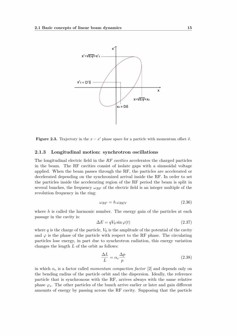
At CERN, the European Organization of Nuclear Research, takes place the world’slargest and most powerful particle accelerator: the Large Hadron Collider (LHC)[10]. It is a circular accelerator designed with the aim of testing the predictionsof The Standard Model particle theory, particularly looking for the theorized, andnow discovered, Higgs boson and possible supersymmetric particles predicted bythe supersymmetry theory. The LHC is located at the Franco-Swiss border nearGeneva and is installed in a 27 km long circular tunnel at a depth ranging from50 to 175m underground. The LHC is capable of accelerating protons and ions.The design centre-of-mass energy for protons and ions collisions is at 14TeV and
Figure 3.1. Layout of the LHC. Four sections host the experiments, other the collimation,the RF and the dump system [8].

24 3. The Large Hadron Collider
1.15PeV respectively. The two beams are bent to stay on their circular orbits bysuper conducting magnets cooled in a bath of superfluid helium to 1.9K degrees.They collide in four detectors of the LHC experiments: ALICE, ATLAS, CMS andLHCb. Since 2010 the LHC was running. The first period 2010-2011 at 3.5TeVper beam, then in 2012-2013 the beam energy was increased to 4TeV. The designparameters are not yet achieved and for this reason on March 2013, the LHC hasstarted a shutdown period (LS1) in order to upgrade the machine and make it readyto reach the nominal beam energy. The re-starting of the machine is expected inthe early 2015.
3.1 The accelerator complex
The LHC is the last of a complex accelerator chain ( Fig.3.2 ) that allows to reachthe operation energy for the circulating beams in the LHC ring [11]. After theextraction from the hydrogen source at about 50 keV, the protons enter in the 35mlong LINear ACcelerator (LINAC), where their energy is increased up to 50MeV.After they are injected in the the Proton Synchrotron Booster (PSB) that bringsthem to 1.4GeV. With this energy they are ready to be transferred in to the ProtonSynchrotron (PS) where are grouped into trains of bunches with 25 or 50 ns spacingand they reach the energy of 26GeV. Then, the protons are transferred to the SPS(Super Proton Synchrotron), where they are accelerated up to 450GeV and finallyinjected into LHC split in two beams. The LHC is divided in several insertions (IRs)where all the components and the experiments are installed [13]. The 27 km lengthare divided into eight arcs and eight straight sectors, that consist in 23 FODO cells.The superconducting dipoles of 15m length each, are designed to work with a 8.3Tmagnetic field at the temperature of 1.9K. The two beams (Fig.3.1) are injectedinto the machine in IR2 (Beam 1) and IR8 (Beam 2) and accelerated up to thenominal top energy by the radio frequency cavities located in IR4. The four collisionpoints host the detectors: the two biggest experiments are ATLAS (A ToroidalLHC ApparatuS) [14] (Point 1) and CMS (Compact Muon Solenoid) [15] (Point 5).LHCb (Large Hadron Col- lider beauty) [16] (Point 8) is dedicated to study thedecay of B mesons and ALICE (A Large Ion Collider Experiment) [17] (Point 2) isoptimized for heavy ions collisions. The normal operation of the machine is calledthe Physics period, during which the beams are stored and kept colliding for manyhours. Once the Physics period ends or in case of a failure, a dump system locatedin IR6 extracts the beams from the ring. The insertions IR3 and IR7 are dedicatedto the momentum and betatron cleaning respectively.One of the most critical parameters for a particle collider is the Luminosity. It isdefined by the accelerator parameters, as follows:
L = nbN2b fγ
4πεnβ∗F (3.1)
where Nb is the number of particles per bunch, nb is the number of bunches perbeam, f is the revolution frequency, γ is the relativistic gamma, β∗ the beta functionat the collision points and F the geometric luminosity reduction factor due to thecrossing angle of the colliding bunches. εn = εβrelγrel is called normalized transverse

3.2 The LHC collimation 25
Figure 3.2. Accelerator complex at CERN [12].
beam emittance and it stays constant with the energy. The L allows to calculate theinteraction rate for a certain process: dNp/dt = σp · L, where σp is the process crosssection. The higher is the luminosity, the greater is the number of interesting eventsproduced during each collision. In 2011, with beam energy of 3.5TeV the maximumpeak luminosity arrive to 4×1033 cm−2 s−1. In 2012, with beam energy of 4TeV themaximum peak luminosity arrive to 0.77×1034 cm−2 s−1, still below the designedluminosity of 1034 cm−2 s−1 but allowed to produce enough events to discover theHiggs boson. The main parameters for the nominal proton beam operation areshown in Table 3.1.
3.2 The LHC collimation
The superconducting magnets would quench at 7 TeV even if a small amount of energy(around 30mJ/cm−3, corresponding to a local loss of 4×10⁷ protons) is depositedinto the superconducting magnet coils. Therefore, a very efficient collimation systemis required in order to intercept and absorb any beam losses in a safe and controlledway.

26 3. The Large Hadron Collider
3.2.1 LHC collimator design
The closest parts to the beam are the collimator jaws. Most of the LHC collimatorsconsist in two jaws with the beam passing in the centre between them, see Fig.3.3and 3.4. They are made of different materials, according to their role in the hierarchydiscussed in 2.2.3. The jaw surfaces are constituted by a flat part, determining theactive length (different for each collimator type) and by a 10 cm tapering part at both
Table 3.1. LHC main design parameters from [13]. The table shows the design values ofthe parameters (at injection and collision). The last column contains the values usedduring the 2012 physics operation.
Injection Design 2012collision collision
Beam dataEnergy [GeV] 450 7000 4000Relativistic gamma 479.6 7461 4263Number of particle per bunch 1.15×10¹¹ 1.4×10¹¹
Number of bunches 2808 1380Bunch spacing [ns] 25 50Transversal normalized emittance [µm rad] 3.75 2.5Stored energy per beam [MJ] 23.3 362 146.5Energy loss per turn [eV] 1.15×10⁻¹ 6.71×10³ 0.72×10³
Peak luminosity related dataRMS bunch length [cm] 11.4 7.55 9.73Geometry luminosity reduction factor F - 0.836 0.79Peak luminosity in IP1 and IP5 [cm−2s−1] - 1.0×1034 0.77×1034
GeometryRing circumference [m] 26658.883Ring separation in arcs [mm] 194
MagnetsNumber of main bends [m] 1232Length of main bends [m] 14.3Bending radius [m] 2803.95Field of main bends [T] 0.535 8.33 4.76
LatticeHorizontal tune 64.28 64.31 64.31Vertical tune 59.31 59.32 59.32Momentum compaction αc 3.225×10⁻⁴
Gamma transition γtr 55.68RF system
Revolution frequency [kHz] 11.245RF frequency [MHz] 400.8Harmonic number 35640Total RF voltage [MV] 8 16 12Synchrotron frequency [Hz] 61.8 21.4 26.3

3.2 The LHC collimation 27
Figure 3.3. Scheme of LHC collimator [8].
ends to minimize geometrical impedance effects. An important feature is that theyare movable in order to efficiently intercept the beam halo. Indeed, the collimatorjaws must always be centered and aligned with respect to the beam envelope and theactual orbit. The two collimator jaws are put in a vacuum tank. The cooling of jawsand tanks is provided by a heat exchanger with copper-nickel pipes. The apertureand the tilt angle of the jaw is set by four precise stepping motors per collimator.In addition a fifth motor can shift transversally the whole collimator tank for somespecial collimators. The mechanical stress caused by the contact between materials(jaws and heat exchanger) having different thermal expansion coefficient, is avoidedby a GlidCop support bar that presses the cooling pipes against the jaw material bymeans of clamping springs. This system also enhances the thermal contact betweenthem. Depending on their orientation in the space, collimators can be horizontal,vertical or skew. The azimuthal angle for the skew ones is defined by starting fromthe positive x-axis and rotating clockwise in the x− y plane.One of the most discussed point of the collimator design concerns the choice ofthe material of the jaws. Materials with high atomic number Z, like tungsten, arepreferable to reach a sufficient absorption rate for cleaning task. However they aremuch less robust against mechanical damage than low Z materials (graphite forexample) that are preferred to reduce the power deposition in the jaw. Primary
Table 3.2. Material jaws for different collimator types.
Collimator type Length [m] MaterialPrimary 0.6 CSecondary 1.0 CTertiary 1.0 WAbsorber 1.0 CTCL 1.0 Cu
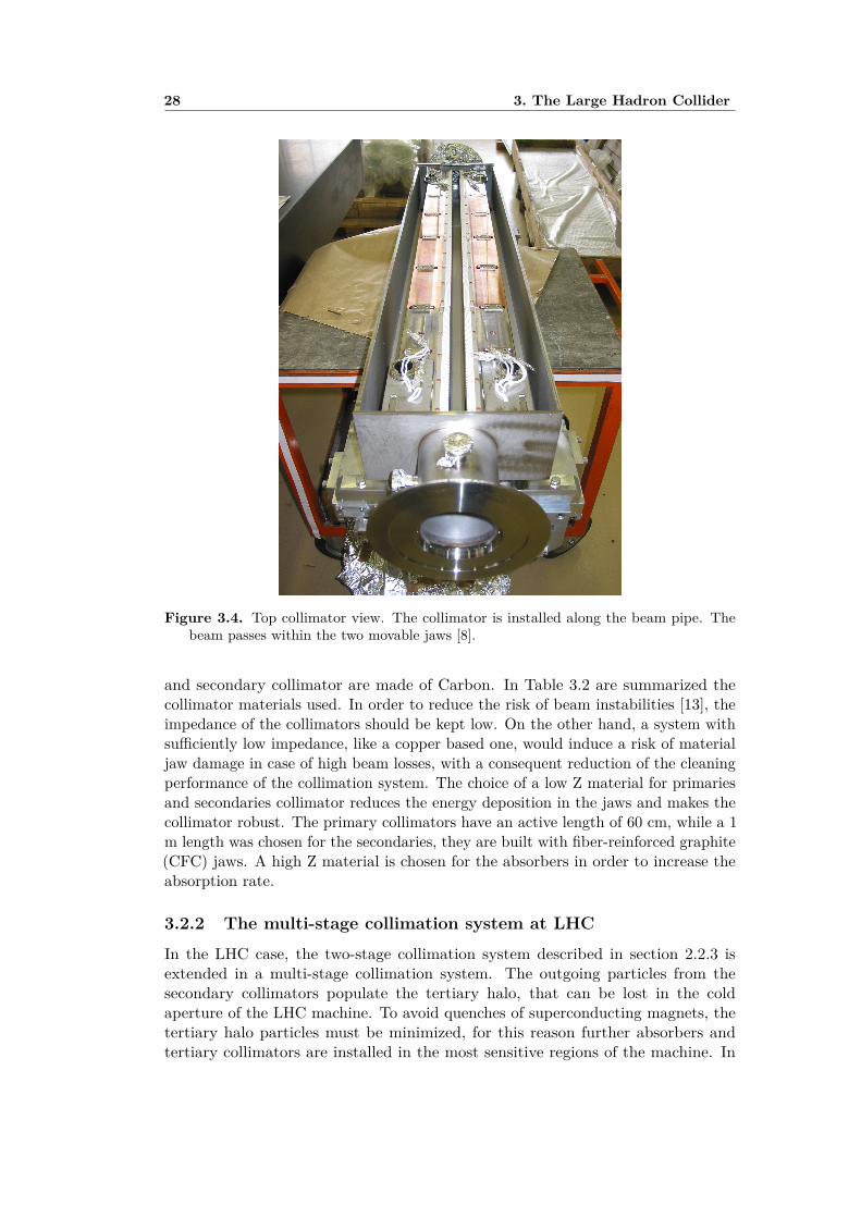
28 3. The Large Hadron Collider
Figure 3.4. Top collimator view. The collimator is installed along the beam pipe. Thebeam passes within the two movable jaws [8].
and secondary collimator are made of Carbon. In Table 3.2 are summarized thecollimator materials used. In order to reduce the risk of beam instabilities [13], theimpedance of the collimators should be kept low. On the other hand, a system withsufficiently low impedance, like a copper based one, would induce a risk of materialjaw damage in case of high beam losses, with a consequent reduction of the cleaningperformance of the collimation system. The choice of a low Z material for primariesand secondaries collimator reduces the energy deposition in the jaws and makes thecollimator robust. The primary collimators have an active length of 60 cm, while a 1m length was chosen for the secondaries, they are built with fiber-reinforced graphite(CFC) jaws. A high Z material is chosen for the absorbers in order to increase theabsorption rate.
3.2.2 The multi-stage collimation system at LHC
In the LHC case, the two-stage collimation system described in section 2.2.3 isextended in a multi-stage collimation system. The outgoing particles from thesecondary collimators populate the tertiary halo, that can be lost in the coldaperture of the LHC machine. To avoid quenches of superconducting magnets, thetertiary halo particles must be minimized, for this reason further absorbers andtertiary collimators are installed in the most sensitive regions of the machine. In

3.2 The LHC collimation 29
Fig.3.5 is shown a schematic view of the LHC multi-stage collimation system.For the beam cleaning is possible to have two different type of cleaning: the betatronand the momentum. The first one allows to limit the transverse extension of thebeam halo by removing particles with high betatron amplitude. The second oneremoves the halo particles that perform large synchrotron oscillations having a largemomentum deviation respect to the reference particle. In the case of LHC, there aretwo different insertions that fulfill the two task separately. Fig.3.6 shows a completelayout (not in scale) of all installed collimators in the LHC with the insertionsdedicated to the betatron and momentum cleaning:
• Betratron cleaning insertion (IR7): this point of the machine is characterizedby low dispersion value and so the transversal shift due to the momentumoffset is negligible. In this way the particles at large distance from the beamhave a high betatronic amplitude mostly.
• Momentum Cleaning insertion (IR3): here the dispersion is higher and thehalo particles have a high momentum offset. This insertion, due to opticsconstraints, the β−function is not negligible in IR3.
Both the momentum cleaning and the betatron cleaning are performed in the LHCwith the multi-stage collimation system.
Figure 3.5. Schematic layout of the LHC multi-stage collimation system [18].
3.2.3 Collimator layout for beam cleaning and experiments protec-tion
The LHC collimator hierarchy consists in primary (TCP) and secondary (TCSG)collimators and tertiary (TCLA). At LHC energies, the TCP cannot absorb allprotons from the primary halo and a secondary halo leaks out. Secondary collimators(TCSGs), downstream of the TCPs and more open, intercept it. The TCLAs aremore open than the TCSGs and must intercept the particles even farther away

30 3. The Large Hadron Collider
Figure 3.6. General collimators layout and cleaning insertions of LHC [5].
from the core (tertiary halo) and the showers produced by inelastic interactions ofthe protons inside the TCP and the TCSG jaws. The collimator settings with thehalf-gap positions for different beam energies are shown in Table 3.3.Some special collimators are installed in the most critical location of the ring.In order to protect the LHC against possible losses following equipment failuresor wrong operation. The injector beam stoppers (TDIs) are vertical collimatorsmade of carbon-carbon jaws of 4.2m length. They are installed to ensure a correctbeam injection setup even in case some of the injector kickers fails: the upper jaw,intercepts particles not sufficiently deflected by the kickers, while the lower jawcatches miskicked beam. In addition, TCLI two-sided vertical collimators are locatedin IR2 for Beam 1 and IR8 for Beam 2. This type of collimator are moved in whenthe beam is injected and then retracted before the particle acceleration. In IR6, adump protection collimator, called TCDQs, is placed, followed by a TCSG that, incase of malfunctioning of the beam extraction system, protects the machine. TheTCDQs are several one-side horizontal collimators of 3m length.Tertiary collimators TCTH (horizontal) and TCTV (vertical) are installed upstreamof the triplet magnets near the experimental points. The triplets are quadrupolesused to reduce the beta function at the collision points (IR1, IR2, IR5 and IR8). TheTCTs provide protection during the squeeze of the beam and the collision and alsoreduce the halo related background in the detectors. They are two sided collimatorswith 1 m tungsten jaws. Copper absorbers (TCL) protect the machine from particleshowers (debris) coming from the collisions in IR1 and IR5, where high luminosity is

3.2 The LHC collimation 31
Table 3.3. Collimator settings for the different families in the cleaning hierarchy, expressedin units of the beam size σ, at different energies: 450GeV (injection), 4TeV (top energyin 2012), 7TeV (expected top energy after long shutdown) assuming εnorm=3.5 µm rad.
half-gap[σ]450 [GeV] 4 [TeV] 7 [TeV]
IR3 TCP 8.0 12 15TCSG 9.3 15.6 18TCSM open open openTCLA 10 17.6 20
IR7 TCP 5.7 4.3 6.0TCSG 6.7 6.3 7.0TCSM open open openTCLA 10 8.3 10
IR6 TCDQ 8.0 7.6 8.0TCSG 7.0 7.1 7.5
IR1 TCTH 13 9.0 8.3TCTV 13 9.0 8.3
IR2 TCTH 13 12 25TCTV 25 12 25TCLI 7.0 open openTDI 6.8 open open
IR5 TCTH 13 9.0 8.3TCTV 13 9.0 8.3TCLP 25 10 15
IR8 TCTH 13 12 25TCTV 13 12 25TCLI 7.0 open openTDI 6.8 open open
TCXRP open open openTCRYO open open open
reached. After the energy ramp, the beam is squeezed in preparation of the physicsoperation. Unlike the other collimators, the TCTs are also moved in during thesqueeze.


33
Chapter 4
Collimation cleaning setup
SixTrack is a code written in Fortran-77 used for collimation and beam cleaningstudies [19]. The first purpose of SixTrack was to study non linearities and dynamicaperture in circular machines tracking pairs of particles through an acceleratorstructure over a large number of turns. Aftertwords, the SixTrack code was extendedin a new sophisticated version which tracks a large number of halo particles interactingwith the collimators [20].
4.1 SixTrack for collimation
The SixTrack code treats the six-dimensional vectors of coordinates (x, x′, y, y′, s, E),where the s coordinate is the longitudinal position (parallel to the beam direction), Eis the energy of the proton, x and y are the perpendicular coordinates to s and x′ andy′ the angles (Fig.2.1). It is based on an element-by-element tracking using transfermatrices to describe the effect of each lattice element. With a magnet system model itconsiders the non-linearities up to the 20th order. The new SixTrack version includesthe COLLTRACK/K2 program. The K2 code was developed during the 1990’s forLHC collimation studies [21]. It is a scattering routine based on a Monte Carlomethod that simulates all the physical interactions between the hitting particle andthe matter of the collimator jaw. After the end of 2000 the K2 routines were includedinto the COLLTRACK program which allows to track few millions of particles overhundreds of turns for different halo types and simulate proton scattering processesin various collimator materials, including point-like elastic and inelastic interactionsand single-diffractive events. The COLLTRACK/K2 is implemented as a part ofthe SixTrack source code and this updated version is nowadays the main tool fortracking particles and collimation studies for LHC.
4.2 Particle Tracking
During a SixTrack run, the particles are tracked through the lattice element byelement. Their coordinates are transformed according to the type of element usinga map derived from the electromagnetic field [4]. The machine optics layout isdefined by the MAD-X program [22]. To calculate the LHC optics it requires thespecification of some parameters such as the magnetic strength and sequence of the

34 4. Collimation cleaning setup
machine elements (including collimators) for the tracked beam (Beam 1 or Beam2), beam energy, type of tracked particles, crossing and separation schemes at theinteraction points. The lattice of the machine is approximated by the model calledthin lens. The lattice elements have no longitudinal extension and is schematicallyrepresented by a marker located at the centre of the elements itself. The wholeelement length is replaced by a drift space and the distance between two consecutivecomponents is given by the real distance between them plus the half length, seeFig.4.1. The thin lens formalism is used to reduce the CPU effort that would occuras a result of thick-lens tracking. In some cases, in order to increase the precisionfor a thick element is possible to split it in several thin lenses.
Figure 4.1. The thin lens formalism. On the top, an element in the lattice, on the bottomthe same element in the thin lens scheme.
4.3 Input files to run SixTrack
The latest version of the SixTrack source code for collimation studies can be foundat: SixTrack code web-page.To perform SixTrack simulations are needed specific input files containing detailsabout:
• machine lattice, in particular magnetic strength and sequence of the machineelements (including collimators)
• collimator properties: name, opening, length, material, rotation angle, offsetand β-function at collimators
• SixTrack setting with the main tracking parameters such as maximum numberof turns, number of particles and energy.

4.3 Input files to run SixTrack 35
Figure 4.2. Fragment of the fort.2 file used to describe the geometry and strengthparameters in SixTrack.
4.3.1 Machine lattice
The machine lattice can be provided to SixTrack through the input file fort.2. For thework presented here, this file is obtained by running MAD-X using the LHC officiallayout [22]. This is the standard tool to describe particle accelerators, simulate beamdynamics and optimize beam optics. The command: "sixtrack, radius=17E-03 ",generates a file called fc.2 with the basic structure of the lattice. This file, renamedas fort.2 [19], is used by SixTrack for the element-by-element tracking. Fig.4.2 showsa section of the fort.2 file. MAD-X dumps all the consecutive linear element in onebloc and all the non linear elements in-between. The single element properties areread by parsing the fort.2 file. The first column is the name of the element, and theother the element properties.
4.3.2 Collimator properties
In the case of running SixTrack for collimation studies, a collimator database, contain-ing the details of all the collimators, is also read. This file is called CollDB_2012_b1for Beam 1, and CollDB_2012_b2 for Beam 2, it contains the following information:
• Total number of collimators
• Collimator name
• Collimator setting expressed in σ units from the beam centre (this parameterscan be also setup later in the fort.3 file, if so, the setting here will be ignored)
• Collimator jaw material:
• Jaw active length [m]
• Azimutal angle [rad] of collimator jaws
• Transverse collimator gap offset respect to the centre of the beam orbit [m]
• The Twiss parameter βx and βy [m] at the collimator location
Fig.4.3 shows a section of this file.

36 4. Collimation cleaning setup
Table 4.1. Collimator materials and densities implemented in SixTrack.
Material Density [g cm−3]C=Carbon 2.26 (1.65)1
C2=Carbon 4.52BE=Beryllium 1.848AL=Aluminum 2.70CU=Copper 8.96W=Tungsten 19.3PB=Lead 11.351 This density is implemented in the new Six-
Track version (see Chap.5).
4.3.3 SixTrack setting file
SixTrack setting and the main tracking parameters are set up in the fort.3 file. Itcontains the number of particles to be tracked, given as a multiple of 64, the beamenergy, the emittance both in the horizontal and vertical plane and the halo typedistribution. The tracking can be performed for a beam halo generated in the thechosen plane (horizontal or vertical) with a smear ±δAx,y around the normalizedamplitude Ax,y in σ units. The smear gives information about the "thickness" of thehalo. Therefore, no computing time is lost tracking the beam core. In this file ispossible to choose one of the following halo distributions [8]:
1. Flat distribution in the selected plane between Ax± δx (horizontal) or Ay ± δy(vertical). The amplitude in the other plane is zero.
2. Flat distribution in the selected plane with a Gaussian distribution cut at 3σin the other plane. This is illustrated in Fig.4.4 where on the left is shown thedistribution in the phase space plane (x − x′) and (y − y′) and on the rightthe distribution in the transverse plane (x− y). In particular, this case is usedin the simulations presented here.
3. Flat distribution in the selected plane plus a Gaussian distribution cut at 3σin the other plane, with an energy spread and a longitudinal bunch lengthdefined.
4. Halo distribution read from an external file.
5. Radial transverse distribution of radius Ar that corresponds to a flat distribu-tion both in the horizontal and vertical planes with Ax = Ay = Ar/
√2
In addition is possible to use the pencil-beam configuration on the selected collimator.In this case is possible define the desired impact parameter in sigma units on thecollimator selected, the offset and the energy spread of the halo particle. Thedistribution types available for the pencil-beam case are: pencil-like distribution,rectangular beam, Gaussian beam both in x and y directions and rectangular beamin x and Gaussian in y.

4.4 Post processing and simulation outputs 37
Figure 4.3. Fragment of the collimator database file with the tracking parameters andcollimator setting.
In the fort.3 file is also possible to select the collimator setting (in sigma units)instead of using the collimator database. In Fig.4.5 is shown a section of the fort.3file.
Figure 4.4. Halo distribution in the phase space (x− x′)and (y − y′) and transverse plane(x−y) for the case of a flat distribution in the selected plane with a Gaussian distributioncut at 3σ in the other plane [5].
4.4 Post processing and simulation outputs
SixTrack computes the trajectories of the halo particles along the accelerator machineby using the six-dimensional phase space coordinates (x, x′, y, y′, s, E). The particlesinteract with the collimator and they are tracked until an inelastic scattering occurswithin the jaw. Scattered particle trajectories are stored in the tracks2.dat file. Thetransverse coordinates information about the inelastic interactions occurred are

38 4. Collimation cleaning setup
Figure 4.5. Extract from the fort.3 input file to the SixTrack collimation routine
contained in the FLUKA_impacts.dat file. The FirstImpacts.dat file contains thetransverse and longitudinal coordinates at the entrance and at the end of the jawfor the ingoing and outgoing protons that hit the collimator for the first time. Thisfile contains also the impact parameter b defined as the transverse offset between theimpact location and the edge of the jaw. A summary of the number of impacts onthe jaw and absorbed protons for each collimator, is given by the output file collsummary.dat. The information related to the collimator setting and main opticsparameters at the collimators are listed in the collgaps.dat file, in addition theefficiency.dat file contains the global cleaning efficiency data defined in Eq.2.47.In order to localize the losses along the LHC ring, a post processing comparisonbetween the aperture model, not including collimators and protection elements, andthe particle trajectories from the SixTrack output file tracks2.dat is needed. Thiscomparison is performed by the BeamLossPattern program that permits to identifyloss locations with an arbitrary resolution ∆s. Then is generated the output fileLPI_PartLost.dat with 10 cm resolution. In Fig.4.6 is shown an example of a particletrajectory in the LHC aperture model. By using the LPI_PartLost.dat file anotherprogram called CleanInelastic cleans up the FLUKA_impacts.dat from the fakeabsorptions due to particles formerly lost in the machine aperture and keeps only theinformation about particles absorbed in the collimator jaws. Then a new file, calledimpacts_real.dat is generated. This is the main input for energy deposition andbackground studies performed by the FLUKA code [24, 25, 26]. FLUKA programcalculates the showers of particles generated by the inelastic interactions of theprimary protons with the different collimator jaw materials.

4.5 SixTrack reference plots for collimation studies 39
Figure 4.6. Example of a trajectory of a particle lost in the LHC aperture [23]
4.5 SixTrack reference plots for collimation studiesSixTrack is a complex software, when it is run for collimation studies, the usercan configure many parameters such as: the machine layout, collimator setting,beam halo, etc... In order to validate the code that is being used and check theinput parameters, we have developed a Python software library to generate a set ofreference plots. This can be useful for several reasons:
• to validate changes made on local private versions,
• to verify different kind of input parameters,
• for comparisons with other tracking routines and
• as a starting point for new user on SixTrack simulations.
A summary of the reference plot types with the respective files needed is shown inFig.4.7. In the next sections will be presented the most relevant reference plots.
Figure 4.7. Summary list of reference plots with the SixTrack output files to generatethem.

40 4. Collimation cleaning setup
Figure 4.8. Collimator setting with the half-gap in σ units for the 7TeV case.
4.5.1 Collimator setting and layout
As discussed in section 4.1.3, from the collgaps.dat file is possible to collect infor-mation about the collimators used. In particular, it contains the IDs to identifythe collimators, the rotation angle of each collimator, the βx and βy (expressed inmeters) at the collimator location, the half-gap both in meters and σ units, the jawmaterial and the collimator length, the tilt angles and the σx and σy (in meters) atthe collimator. The reference plot in Fig.4.8 shows the complete 7TeV collimatorsettings, the collimators with a half-gap larger than 25σ are totally open. Thissetting corresponds to the nominal configuration shown in Table 3.3 The completecollimator layout for the same energy beam is represented in fig.4.9. It shows theposition along the LHC ring of each collimator used.
Figure 4.9. Collimator layout for Beam 1 4TeV.
4.5.2 Distribution of the generated beam halo
SixTrack performs the tracking for several types of halo distributions (see section4.3.3).The halo type selected in the fort.3 file is generated at IP1 and the spatialcoordinates and angle of the distribution are contained in the output file calleddist0.dat. Fig.4.10a illustrates the circular halo crown and the Gaussian cut at 3σ inthe other plane, for Beam 1 at 7TeV. In particular, are represented the phase spacesx− x′ and y − y′ with the x′ and y′ projections. The spatial coordinates and theangles are normalized to the σx,y and σ′x,y calculated by using Eq.2.18 and Eq.2.19respectively. In this case the β-function at IP1 is β = β∗ = 0.55m. Fig.4.10b shows

4.5 SixTrack reference plots for collimation studies 41
the transverse halo distribution in the x− y plane and the projections in x and ydirections. The transverse coordinates are normalized to the σx,y at IP1 as above.
(a) Halo generated in the x-x’ and y-y’ spaces with x’ and y’ projections.
(b) Transverse distribution of the halo generate and projections in x and y directions.
Figure 4.10. Particle distribution in different spaces: horizontal halo in the x− y planewith annular distribution in the x − x′ phase space and Gaussian distribution in they − y′ phase.
4.5.3 Distribution of impacts at primary collimators
The reference plots that show the impacts at the collimator have been made for twodifferent cases:
• first impacts of the halo particles at the primary collimators
• all impacts of the protons at the different collimators.
The halo particles hit the collimator with a certain impact parameter b, defined asthe transverse offset between the jaw surface and the impact point. It is a positivevalue, typically in the range of 0<b<100µm at the first impact. By using theinformation contained in the First_impacts.dat file, such as the impact parametersand the ingoing coordinates at the collimator, is possible to draw the plot in Fig.4.11.It shows, for the horizontal halo case (Beam 1 at 7TeV), the transverse distributionof the first impacts on the primary collimators. In this case, the x position is alwayspositive, because it represents the impact parameter on the collimator jaw. Thex and y coordinates are normalized by using Eq.2.18 and Eq.2.19 with the γ andβ values at primary collimator locations. Because the halo generated is in thehorizontal plane, there is not any hits on the vertical primary collimator, howeversome of the halo particles hit the corner side of the skew collimator. The impactsshape on the skew primary collimator is geometrical explained in the Fig.4.11c.
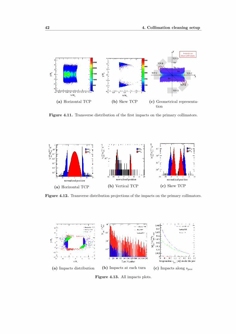
42 4. Collimation cleaning setup
(a) Horizontal TCP (b) Skew TCP (c) Geometrical representa-tion
Figure 4.11. Transverse distribution of the first impacts on the primary collimators.
(a) Horizontal TCP (b) Vertical TCP (c) Skew TCP
Figure 4.12. Transverse distribution projections of the impacts on the primary collimators.
(a) Impacts distribution (b) Impacts at each turn (c) Impacts along spos
Figure 4.13. All impacts plots.

4.5 SixTrack reference plots for collimation studies 43
Up to now we show the distributions of the first impacts. However, particles can hitseveral collimators before being absorbed or lost in the aperture. Fig.4.13a shows allthe impacts at the three primary collimators in IR7, in red for the vertical planeand blue for the horizontal plane.The difference is now that particles scattered inthe horizontal or skew collimator can reach the vertical collimator and thus we seethe impacts in Fig.7.11b The number of particle absorbed at each collimator N coll
abs isnormalized to the collimator length Lcoll and to the total number of particles absorbedNTOTabs . Fig.4.13a shows the superposition of all the impacts at the three TCP in
IR7. The different colors represent the three primary collimators: horizontal (blue),vertical (red) and skew (green). The impacts_real.dat file contains also informationabout the turn during which the proton is lost at the collimator. Fig.4.13b showsthe number of particle absorbed at the primary collimators per turn. The impactsalong the longitudinal s position is shown in Fig.4.13c.
4.5.4 Distribution of impacts at TCTs and dump protection
The experimental insertions host horizontal (TCTH) and vertical (TCTV) tertiarycollimators to provide protection to the triplet magnets. The triplets are assemblyof three quadrupole magnets used to reduce the optical β-function at the collisionpoints. The LHC machine has triplets in IR1, IR2, IR5 and IR8 insertions.The tertiary collimators are two-sided collimators formed by 1m copper jaws with atungsten inlay. For 7TeV simulations, with β∗ of 0.55m, they are set at 8.3σ in IR1and IR5, while more relaxed gaps at 25σ are used for the TCTs in IR2 and IR8,with β∗ of 10m.The dump system is installed in the extraction region in IR6, where the TCDQsabsorb the beam swept over the machine aperture in order to avoid radiationdamage. One horizontal TCSG collimator is located next to TCDQs to providefurther protection to the downstream machine elements. In order to check and verifythe simulation results, Fig.4.14 shows the number of impacts on tertiary collimatorsin IP1, IP2, IP5, IP8 and in the dump protection system in IP6. The losses arenormalized to the total number of particles absorbed for Beam 1 horizontal halocase at 7TeV.
Figure 4.14. Number of absorbed particles at different IP collimators, normalized to thetotal number of absorbed particles.

44 4. Collimation cleaning setup
4.5.5 Particle lost at aperture in the Dispersion Suppression regionat IR7
The IR7 insertion contains the betatron cleaning system where the particles withlarge betatron amplitude in both vertical and horizontal directions are scatteredby the primary collimator jaws and absorbed by the secondary collimators. Themost critical area in terms of losses is the region downstream of IP7 (for Beam 1)that is called the Dispersion Suppressor (DS). This region consists in a lattice cellswith one dipole magnet missing, reducing so the dispersion function. The dispersionsuppression regions are located at the end of each LHC arc and the tunnel geometrydetermines their lengths. A plot that shows the transverse distribution of the lossesin the DS region, in the range of 20270-20350m, with the projections in the x and ydirections, is shown in Fig.4.15. The curved shape profile shows the simulated beampipe.
(a) Transverse distribution (b) Transverse distribution projections
Figure 4.15. Distribution of the particle lost in the aperture of the DS region in IR7.
4.5.6 Standard loss maps and cleaning efficiency
The SixTrack simulation results allow to draw detailed maps of loss location along thewhole LHC ring, for different optics and collimator settings, by using specific SixTrackoutputs file. In particular, reading the impacts_real.dat is possible to calculatethe particles absorbed at the collimators, while by reading the LPI_PartLost.datis possible to compute the number of particles lost at the machine apertures.These detailed maps are called beam loss maps and show the local cleaning inefficiencyηc, defined in Eq.2.48, along the length of the machine with a ∆s=10 cm resolution.An example of a loss map is shown in Fig.4.16 for Beam 1 horizontal halo case at7TeV. The red lines, called warm losses, identify beam losses in normal conductingmagnets that work at room-temperature. The blue lines represent the cold lossesthat show the location of proton losses in superconducting magnets. In order toprevent the quench of the superconducting magnets, the cold losses must not exceedthe quench limit defined in Eq.2.49. The cleaning inefficiency at the collimatorsare represented by the black lines. In the case of collimators the resolution ∆sin the cleaning inefficiency definition is substituted by the collimator jaw activelength. For this reason at the primary collimators, with a 0.6m jaw length, thecleaning inefficiency can be greater than one. Fig.4.16b shows a zoom of the betatron
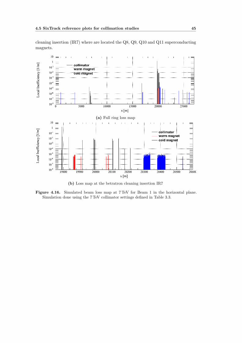
4.5 SixTrack reference plots for collimation studies 45
cleaning insertion (IR7) where are located the Q8, Q9, Q10 and Q11 superconductingmagnets.
(a) Full ring loss map
(b) Loss map at the betratron cleaning insertion IR7
Figure 4.16. Simulated beam loss map at 7TeV for Beam 1 in the horizontal plane.Simulation done using the 7TeV collimator settings defined in Table 3.3.


47
Chapter 5
Improved physics model forSixTrack scattering routine
The high energy proton beams of the LHC interact with the matter of the collimatorjaws through scattering mechanisms due to interactions of the incoming protonswith either the electro-magnetic field of the atoms or the strong potential of thenucleus [27]. The scattering mechanisms are modeled and implemented in SixTrackwith a Monte-Carlo code deriving from the K2 scattering routine. The K2 is asoftware package, developed during the 1990’s by T.Tranker and J.B Jeanneret [21],for setting up and testing collimation systems in circular accelerators for protonbeams.In this code we classify the interactions between a high energy proton and the matteras follow:
• Nuclear interaction, with a finite cross sections:
– inelastic scattering with the nucleus of total cross section σinpN– elastic scattering with the nucleus of total cross section σelpN– scattering with whole nucleus of total cross section σtotpN– proton-nucleon elastic scattering of total cross section σelpp– single diffractive scattering of total cross section σSDpp
The inelastic interactions produce a variety of lower energy particles that arelost within the nearest collimation section. Instead, the other interactionsleave the energy of the particle in a range that is well accepted by the opticsof the accelerator.
• Coulomb scattering, a stochastic process that occurs when the incoming particlehas a large impact parameter. The incoming particle feels the long rangeoverlapping fields of all ions or molecules and is kicked by small angles. Onlyif the particle gets closer to an ion, it is scattered with a substantial kickdescribed by the Rutherford scattering formula. Thus the Coulomb scatteringcan be described in two different ways:
– Large angle Rutherford scattering with a finite cross section, σRth, forparticles that have small impact parameter on the ions and

48 5. Improved physics model for SixTrack scattering routine
– Multiple Coulomb scattering (mCs) described as a stochastic process forparticles that have a long range interaction
.• Ionization: the electrons of the atomic shells are kicked off because of the
energy released by the passing particle. The particle loses a small amount ofenergy proportional to the length of the traversed matter.
• Hard electro-magnetic processes like pair production: these processes aremarginal below 10 TeV and are not implemented in the Monte-Carlo code.
The cross sections of the SixTrack scattering routine have been updated taking intoaccount recent experimental data. In addition, other improvements were carried outin order to describe better the interaction processes. All of them will be presented inthe next sections with a brief theoretical description followed by the changes carriedout on the routine.
5.1 SixTrack scattering routineThe scattering routine of SixTrack is divided in different subroutines, each one witha specific purpose. An overview of the calling sequence between the subroutines isshown in Fig.5.1. The starting point to simulate the proton scattering within thecollimator jaw, is established only whether the proton hits the collimator. This isdetermined in the subroutine called Collimate2. Considering now the x-coordinateas: x = |x−half-gapcoll| in the collimator frame (see Fig.5.2) a particle that hasx ≥ 0 surely hits the collimator, that for definition is at x ≥ 0, in this case theproton sees all the jaw length (see Fig.5.2 (1)). When x < 0 and x′ ≤ 0 the protondoesn’t hit the collimator while in case of x′ > 0 and x < 0 the proton hits the edgeof the jaw and the longitudinal s position of entrance must be calculated.
Figure 5.1. Scheme of the calls between different subroutines in SixTrack scattering routine.

5.1 SixTrack scattering routine 49
Figure 5.2. Representation of particle position close to collimator jaw.
In the first case Fig.5.2 (1) the impacting particle sees a collimator of full lengthL. However, in the second case, Fig.5.2 (2) the particle sees only a section of thecollimator length (L− x
x′ ). If s results to be greater than the collimator length itmeans that the proton is passing above the edge of the collimator.In the subroutine called scatin the cross sections are initialized in two-dimensionalarrays that contain both the interaction type and the collimator material (Beryllium,Aluminum, Copper, Tungsten, Lead, Carbon and special carbon fibers).The interactions between the proton and the matter of jaw are implemented in themain subroutine called jaw. In this subroutine the interaction length is randomlygenerated several times, until the proton is absorbed or leaves the collimator jaw.The proton travels the entire interaction length doing multiple scattering and losingenergy by ionization. The rms angle kick due to multiple Coulomb scatteringis computed by the subroutine mcs and the energy lost per unit length, dp/dx,is calculated by the function get_dpodx that has been implemented in the newSixTrack version to calculate the Bethe-Bloch equation. At the end of the path,the function ichoix chooses the kind of interaction occurred by using a cumulativeprobability evaluated from the cross section value. Afterwards, the function gettrangenerates randomly the Mandelstam variable t = (pθ)2 for the selected processand from it the subroutine tetat calculates the angle θ and its projections in thex direction and y directions, in order to apply the angle changes. If an inelasticprocess occurs, the particle is lost at the collimator, otherwise another Monte-Carlo

50 5. Improved physics model for SixTrack scattering routine
interaction length is generated and the proton continues to travel along the jaw.The method is iterated until the interaction length generated is greater than theremaining length of the collimator, the proton does multiple Coulomb scatteringuntil the end of the jaw: this is the last step of the scattering routine.
5.2 Electromagnetic processes
A charged heavy particle, as the proton, moving inside matter loses energy mainlydue to the excitation and ionization of the medium atoms [27, 28]. This type ofinteractions are processes mediated by the electromagnetic field associated to theincoming charged particle and the medium targets. In addition to the energy releasedelectromagnetically, there are effects that occur for approaching distances smallerthan the atomic radius. In this case the transferred momentum is usually very smallrespect to the particle momentum. The charged particle traversing the mediumundergoes a lot of deflections of its trajectory due to the elastic scattering with thenuclei, this process is known as multiple Coulomb scattering.
5.2.1 Ionization
For relativistic charged particles, other than electrons, and neglecting radiativeeffects the mean rate of energy lost by ionization is given by the Bethe-Bloch formula(1930)[27, 29]:
−dEdx
= Kz2Z
A
1β2
[12 ln
2mec2β2γ2TmaxI2 − β2 − δ
2
](5.1)
where me is the electron mass, Z and A are the atomic number and the atomicmass of the medium. The quantities β and γ are the kinematic variables. The meanexcitation energy I is an empirical value given by (10± 1 eV ) ·Z for elements heavierthan the oxygen. Tmax is the maximum kinetic energy that can be imparted to afree electron in a single collision. The last term in Eq.5.1, δ/2 is the so called densityeffect correction.
Figure 5.3. Implemented Bethe-Bloch formula in the case of Aluminum compared withthe previous SixTrack reference value used for simulations.

5.2 Electromagnetic processes 51
The new function get_dpodx has been implemented in order to calculate the Bethe-Bloch equation 5.1. In the previous version, the values of energy lost by ionizationwere taken at the same reference energy Eref=450GeV for different materials. Tobetter evaluate the energy loss rate dE/dx, the function 5.1 is now computed forprotons of any given energy. This evaluation is performed after a conversion to metricunits by using the material density. Fig.5.3 shows the Aluminum energy lost byionization calculated with the function get_dpodx in SixTrack for any given energy.The previous reference value at Eref=450GeV used for the simulations at any energyis also shown with the dashed red line. Table 5.1 quantifies the differences betweenthe two implementations. In the first column are shown the predicted energy lost fordifferent materials with the old routine. Then the next column shows the result ofthe new implementation using the complete Bethe-Bloch equation. The last columnshows the relative difference. Notice that in the previous routine the energy loss wasalways overestimated. The smaller difference is for Aluminum, 13%, and the largestfor Tungsten of up to 30%.
5.2.2 Multiple Coulomb Scattering
A charged particle passing through a thickness of material is subject to a largenumber of small angle deflections all along its trajectory in the medium. Thesedeflections have a stochastic characterization and are due to Coulomb scatteringwith nuclei, so called multiple Coulomb scattering (mCs). The Coulomb scatteringdistribution is well represented by the Moliere’s theory [30] that deals with smallscattering angles.The distribution function f(x, x′, s) for the scattered particle obeys the Fokker-Plankequation, derived and solved by Fermi [31] [32]:
∂sf + x′∂xf = θ202 ∂x
′∂x′f (5.2)
f represents the probability for the charged particle to be in a certain position x inthe transverse direction with an angular deflection x′ after traversing a thickness sof material. θ0 is the rms angular kick received by the particle in the x directionwhen it traverses a unit of length of matter:
θ0 = 13.6MeV
βcpz
1√χ0
(5.3)
Material dE/dx [GeV/m] dE/dx [GeV/m] Relativeat E = 450GeV at E = 7TeV difference [%]
Beryllium (Be) 0.55 0.45 18Aluminum (Al) 0.81 0.71 13Copper (Cu) 2.69 2.15 20Tungsten (W) 5.79 4.0 30Lead (Pb) 3.4 2.36 30Carbon (C) 0.75 0.62 18
Table 5.1. Loss energy rate for Eref = 450GeV previously tabulated in SixTrack and newvalues calculated with the new Bethe-Bloch function at E = 7TeV.

52 5. Improved physics model for SixTrack scattering routine
Figure 5.4. Schematic view of MCS in one plane [27].
βc is the velocity of the incoming proton, z the electronic charge of the beam, p themomentum and χ0 the radiation length of the traversed material. The rms angleafter traversing a length s of matter is:
θ(s) = θ0√s. (5.4)
For a point-like initial distribution represented by:
f(s = 0, x, x′) = δ(x− x0)δ(x′ − x′0), (5.5)
the solution of (5.2) is the Fermi distribution:
f(s, x, x′) =√
3πθ2
0s2 · exp
[− 6θ2
0s3
(x− x0 − sx′0 −
s
2(x′ − x′0)2)]· exp
[− 1
2θ20s(x− x′0)2
](5.6)
The equation (5.3) fails to describe multiple Coulomb scattering when the processesis no more stochastic, as in the case of short length of traversed matter, moreover ifthe incoming proton has a small impact parameter on the nucleus, the Rutherfordscattering occurs and the scattering angles are greater than a few of θ0.Measures on the rms kick lead to the following correct formula:
θ0 = 13.6MeV
βcpz
1√χ0
[1 + 0.038 ln(s/χ0)] (5.7)
which differs from the previous one by the logarithmic term. The rms width is aGaussian approximation for the central 98% of the projected angular distribution.For Monte-Carlo generation of a joint of (x, x′) is convenient to work with twoindependent Gaussian random variables (z1, z2) with mean zero and variance one,and then set:
x = x0 + sx′0 + z1sθ(s)(1− ρ2
xx′)2√
3+ z2ρxxs
θ(s)√3
=
= x0 + sx′0 + z1sθ(s)(z1√12
+ z22 )
(5.8)
x′ = x′0 + θ(s)z2 (5.9)

5.3 Nuclear Interactions 53
where has been used the correlation factor ρxx′ =√
3/2 obtained from the diffusiontheory. This method is used in the Monte-Carlo scattering code to simulate themultiple Coulomb process within the jaw.In the new SixTrack version the mCs Eq.5.3 has been replaced by the Eq.5.7containing the logarithmic part. SixTrack simulations for a horizontal halo of7TeV for different materials of the collimator jaw were carried out to evaluate thedifference with respect to the previous rms angle. In particular, these simulationswere performed considering the passage of protons through a collimator jaw of 0.6mlength. This analysis was performed using the pencil-beam configuration for Beam1. In the selected configuration all the impacting particles have the same energy andthe same angle x′=0 rad. They are centered on the collimator jaw with an impactparameter b=10mm. In Fig.5.5a the θrms(s) angles in the s− x plane calculated bythe Eq.5.3 are shown. The angle is plotted as a function of the s position inside thecollimator jaw for different materials. The dashed lines represent the simulationsperformed without the logarithmic term (old SixTrack), while the solid lines includesthe logarithmic correction (new SixTrack). In the case of light materials, like Carbon,Beryllium, and Aluminum the difference between the two cases can be neglected,while for the heavy materials as Lead, Copper and Tungsten the differences becomenot negligible and can arrive up to 20%. This is shown in Fig.5.5b which shows therelative variation of the θrmsx angle.The angle distribution of the protons at the end of the collimator jaw is shown inFig.5.6. The black line represents the angle distribution from simulations performedwithout the logarithmic term. The wider red line describes the angle distributionafter the correction. A larger spread of the protons outside the collimator can beseen in the latter case. These simulations are carried out for a 60 cm horizontalprimary collimator of Carbon. The relative difference between the rms of the twodistribution is about 17% for Carbon.
5.3 Nuclear Interactions
The incoming protons discretely interact with the nuclei of the material jaw. Eachscattering process is characterized by a finite cross section σ that gives the probabilityfor the process to occur. To specify the cross section and the differential cross sections,related to the probability to find the scattered proton at a given polar angle θ or ata given momentum, the Lorentz-invariant Mandelstam variables are used. Thosevariables for high energy protons are:
• the transverse momentum transferrer t = (pθ)2
• the centre of mass energy squared s ≈ 2mpp
where mp is the proton mass.The total proton-nucleus cross section σtotpN is given by the sum of different contribu-tions as follow [28]:
σtotpN = σinpN + σelpN + σq−elpN . (5.10)
The first term is the inelastic cross section and it gives the probability for theproton to be absorbed by the medium, σelpN refers to coherent elastic scattering with

54 5. Improved physics model for SixTrack scattering routine
(a) Multiple Coulomb scattering angle (rms) in the s-x plane for several material calculatedby using the mCs formula with and without the logarithmic term.
(b) Variation of the mCs rms angle with respect to the formula without the logarithmicpart for different materials.
Figure 5.5. Multiple Coulomb scattering angle (rms) in the (s− x) plane for different pathwith the collimator jaw.
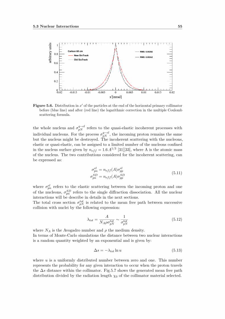
5.3 Nuclear Interactions 55
Figure 5.6. Distribution in x′ of the particles at the end of the horizontal primary collimatorbefore (blue line) and after (red line) the logarithmic correction in the multiple Coulombscattering formula.
the whole nucleus and σq−elpN refers to the quasi-elastic incoherent processes withindividual nucleons. For the process σq−elpN , the incoming proton remains the samebut the nucleus might be destroyed. The incoherent scattering with the nucleons,elastic or quasi-elastic, can be assigned to a limited number of the nucleons confinedin the nucleus surface given by neff = 1.6A1/3 [31][33], where A is the atomic massof the nucleus. The two contributions considered for the incoherent scattering, canbe expressed as:
σelpn = neff (A)σelppσSDpn = neff (A)σSDpp
(5.11)
where σelpn refers to the elastic scattering between the incoming proton and oneof the nucleons, σSDpn refers to the single diffraction dissociation. All the nuclearinteractions will be describe in details in the next sections.The total cross section σtotpN is related to the mean free path between successivecollision with nuclei by the following expression:
λtot = A
NAρσtotpN∼ 1σtotpN
(5.12)
where NA is the Avogadro number and ρ the medium density.In terms of Monte-Carlo simulations the distance between two nuclear interactionsis a random quantity weighted by an exponential and is given by:
∆s = −λtot ln u (5.13)
where u is a uniformly distributed number between zero and one. This numberrepresents the probability for any given interaction to occur when the proton travelsthe ∆s distance within the collimator. Fig.5.7 shows the generated mean free pathdistribution divided by the radiation length χ0 of the collimator material selected.

56 5. Improved physics model for SixTrack scattering routine
5.3.1 Proton-nucleon nuclear scattering
The beam protons are diffused by the nucleons of the matter nuclei by elasticand single diffractive scattering. The experimental data are more abundant andexhaustive for the protons than the neutrons. Since the proton-neutron nuclearscattering is consider equal to the proton-proton scattering, Therefore, the proton-proton quantities will be also used for the proton-neutron case.
Proton-proton elastic scattering
In the previous version of the scattering routine the proton-proton elastic crosssection was calculated using a linear fit from experimental data up to 2.08 · 103 GeVcenter of mass energy.However, the TOTEM collaboration has recently measuredthe proton-proton elastic cross section up to
√s = 8TeV [34]. The measurements of
the proton-proton elastic cross section, proton-proton total cross section and proton-proton inelastic cross section are shown in Fig.5.8 [34]. The new measurementsof the total and elastic proton-proton cross sections at
√s = 8TeV center-of-mass
energy bring the opportunity to perform better fits to the data and therefore improvethe prediction at intermediated energies. In the new SixTrack version has beenimplemented the latest fit from TOTEM measurements for the elastic proton-protoncross section shown in Fig.5.8:
σelpp = 11.7− 1.59 ln s+ 0.134 ln2 s. (5.14)
Notice that since we are simulating high energetic protons into a fixed target (thecollimator jaw), the center-of-mass energy under study is about
√s = 114GeV for
7TeV protons. To determine the momentum change and the angle deflection of thescattered proton the differential cross section has to be known, in first approximationcan be expressed as:
dσ
dt= ae−b(t,s)t (5.15)
where b(t, s) is the elastic slope factor. In the practical t-range considered at theenergy of LHC, the slope factor depends weakly on t, thus can be considered b(s, t) ≈
Figure 5.7. Distribution of the mean free path (λ) divided by the radiation length (χ0) ofthe material chosen, Carbon for the present case.

5.3 Nuclear Interactions 57
Figure 5.8. Elastic, inelastic and total cross sections from TOTEM Collaboration [34].
b(s). In the previous scattering routine was used a parametrization extrapolatedfrom several accelerator experimental data (ISR at CERN, TEVATRON at Fermilab,RHIC at BNL) for energies up to
√s = 200GeV. A new parametrization has
been implemented to extrapolate more accurately the slope parameter value up toLHC energies. Fig.5.9 shows the elastic proton-proton slope factors from severalcollaboration data at different center of mass energies[35] including the recentdata from TOTEM at
√s=7TeV. The dashed blue line represents the fit used
in the previous SixTrack version, the black solid line is the new parametrizationimplemented:
bpp = 7.16 + 1.44 ln√s. (5.16)
At the LHC center of mass energy√s = 114.6GeV, the relative difference between
the previous and the current fit is ∼ 2.5%, this value increases with the centerof mass energy leading to a more realistic description of the proton-proton elasticscattering for proton beams of higher energy.
Single diffractive scattering
The single diffractive scattering (SD) is a low momentum transfer interaction whereone of the protons is coherently excited into a high mass state M without quantumnumber exchange. This process is dominant within a range of excited masses M :
M20 < M2 < 0.15 s (5.17)
where the lower bound is M0 = (mp +mπ) ≈ 1GeV/c2 and 0.15 s is the coherencelimit above which the SD scattering does not occur anymore. The differential crosssection can be parametrized, considering the range of 1 ≤ M2 ≤ 0.15 s, by the

58 5. Improved physics model for SixTrack scattering routine
Figure 5.9. The slope parameter for pp and pp elastic scattering. Data from differentcollaboration including the recent TOTEM measurement [34].
following expression [36]:
dσ2
dtdM2 = Ab(M)e−b(M)
M2 (5.18)
where b(M) is the slope factor and the constant A = 0.68mb. Outside this rangethe cross section is approximately zero.A new model for the total single diffractive cross section has been considered toupdate the previous one based on the standard Pomeron flux [36]. The measurementof the pp single diffraction dissociation cross section at the SppS Collider [37] andat Tevatron [38, 39] led to a phenomenological renormalization scheme for thehadronic diffraction [40]. The new model unitarizes the Pomeron flux factor inthe triple-Pomeron amplitude preserving the M2 and t dependence. Fig.5.10 showsthe total pp and pp single diffractive cross sections data for ξ < 0.05 compared tothe predictions based on the standard and renormalized pomeron flux (from [40]).The quantity ξ ≈ M2/s is the incident proton momentum fraction carried by thePomeron. Fig.5.11 shows the triple-Pomeron Feynman diagram for single diffractionwhere g(t) is the triple-Pomeron (PPP)coupling.Above
√s = 22GeV, where the pomeron flux factor integral becomes unitary, a
linear logarithmic expression has been used in the range 22 <√s < 10000GeV to
obtain the following parameterization for the total single diffractive cross section (inmb):
σSDpp (s) = 4.3 + 0.3 ln s. (5.19)
The single diffractive cross section value extrapolated at LHC energies is predictedby σppsd |ξ<0.05 = 7.15mb at
√s = 114.6GeV for a 7TeV incident proton on a rest
target.The slope parameter b cannot be precisely predicted hence an approximated fit,adjusted on measured data, is used:

5.3 Nuclear Interactions 59
Figure 5.10. Total pp and pp single diffractive cross section data for ξ < 0.05 comparedwith prediction based on the standard and renormalized pomeron flux [40].
Figure 5.11. Triple-pomeron Feynman diagram for single diffraction [40].
b = 2bel M2 < 2GeV (5.20)
b = 136(106− 17M2)bel 2 < M2 < 5GeV (5.21)
b = 712bel M2 > 5GeV. (5.22)
Fig. 5.12 shows the total single diffractive cross section obtained using the previousparameterization (blue line) versus the updated one given by Eq.5.19 (red line).In Table 5.2 the single diffractive cross section values, for different beam energies,calculated by the previous parameterization and the updated one are listed withthe relative variations. For a 7TeV proton beam the relative difference is ∼ 40%, sothe previous SixTrack scattering routine was underestimating the single diffractivecontribution. Further simulations to investigate the effect caused by the high crosssection difference at the injection energy of 450TeV should be performed.

60 5. Improved physics model for SixTrack scattering routine
Figure 5.12. Total single diffractive cross section with the previous parameterization (blueline) and the new one calculated by using the Eq.5.19 (red line)
Table 5.2. Total single diffractive cross section values calculated with the previous parame-terization and the new one.
Momentum p OLD σSD NEW σSD Variation[GeV] [mb] [mb] %450 3.292 6.321 904000 4.778 6.977 507000 5.158 7.145 40
Proton-proton total cross section
The proton-proton total cross section has been updated by using a parametrizationfrom the COMPETE collaboration data fit containing the measured TOTEM proton-proton total cross section at
√s = 7TeV [34]. The fit is shown in Fig.5.8 and it
gives the following total cross section (expressed in mb) :
σtotpp = 41− 2.33 ln s+ 0.315 ln2 s. (5.23)
In Table 5.3 the total proton-proton cross sections from the previous SixTrackimplementation and the new one are presented for several beam energies. The crosssections vary little, the maximum variation is ≈1%.
Table 5.3. Total proton-proton cross sections from the previous SixTrack implementationand the updated one.
Momentum p σtotpp old fit σtotpp new fit Variation[GeV] [mb] [mb] %450 40.0 39.6 14000 45.4 45.3 0.27000 46.9 47.2 0.7

5.3 Nuclear Interactions 61
5.3.2 Proton-nucleus scattering
The beam halo incoming protons are diffracted by the nuclei of the jaw material. Theparticle can interact coherently with the whole nucleus or incoherently with a limitednumber of nucleons neff situated in the nucleus rim. The total proton-nucleus crosssection is:
σtotpN = σinpN + σelpN + σq−elpN . (5.24)
Proton-nucleus elastic scattering
The proton-nucleus elastic cross section is calculated by subtracting all the othercontributions from the total cross section σtotpN .For the differential cross-section dσ/dt the slope factor bpN has been measured forhadron beams on various target materials at different energies [41]. The measuredvalues are reported in Fig.5.13. The A-dependance of the elastic pN scattering slopefactor can be derived from a linear fit on the data:
bpN = 14.1A0.65 (5.25)
this parametrization is used for unmeasured nuclei like Tungsten.
Figure 5.13. Experimental measurements of the slope factor parameter for proton-nucleuselastic scattering bpN versus atomic weight A [31].
Proton-nucleus inelastic scattering
Due to lack of neutron data, the proton measured values are used to calculate theneutron-nucleus inelastic scattering cross section; therefore is assumed σinpN ≈ σinnN .The proton-nucleus inelastic cross section is inherited from the dependence of theσtotpN cross section in the following way:
σinpN = σinpN,ref ·σtotpN
σtotpN,ref(5.26)
The reference proton nucleus inelastic cross section σinpN,ref has been updated usingrecent data of the nuclear interaction length from the Particle Data Group [42].
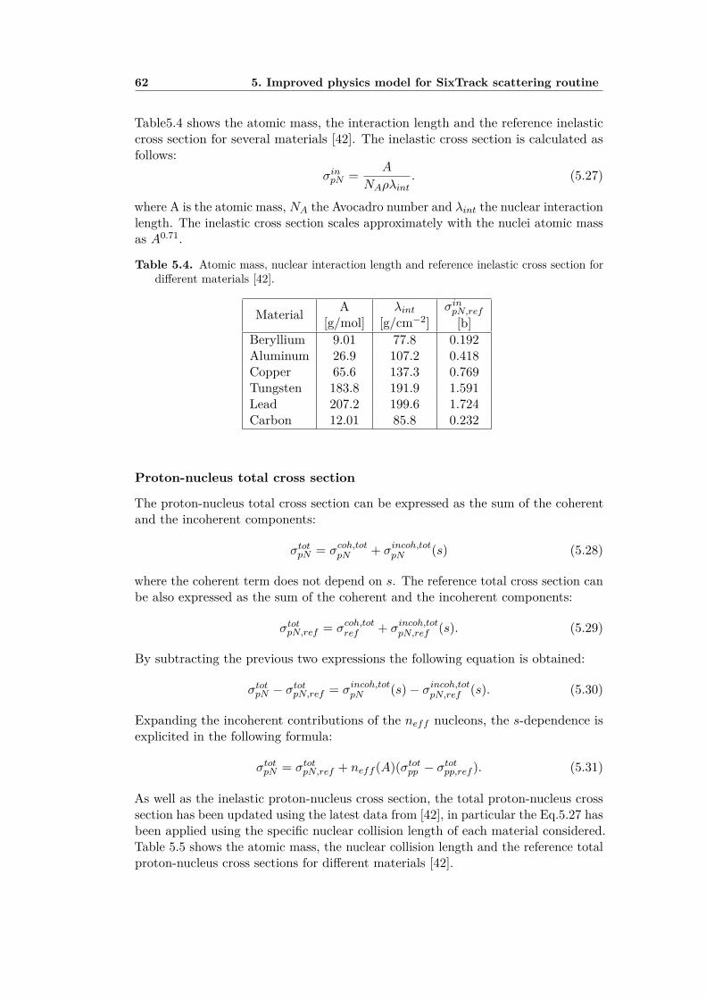
62 5. Improved physics model for SixTrack scattering routine
Table5.4 shows the atomic mass, the interaction length and the reference inelasticcross section for several materials [42]. The inelastic cross section is calculated asfollows:
σinpN = A
NAρλint. (5.27)
where A is the atomic mass, NA the Avocadro number and λint the nuclear interactionlength. The inelastic cross section scales approximately with the nuclei atomic massas A0.71.
Table 5.4. Atomic mass, nuclear interaction length and reference inelastic cross section fordifferent materials [42].
Material A[g/mol]
λint[g/cm−2]
σinpN,ref[b]
Beryllium 9.01 77.8 0.192Aluminum 26.9 107.2 0.418Copper 65.6 137.3 0.769Tungsten 183.8 191.9 1.591Lead 207.2 199.6 1.724Carbon 12.01 85.8 0.232
Proton-nucleus total cross section
The proton-nucleus total cross section can be expressed as the sum of the coherentand the incoherent components:
σtotpN = σcoh,totpN + σincoh,totpN (s) (5.28)
where the coherent term does not depend on s. The reference total cross section canbe also expressed as the sum of the coherent and the incoherent components:
σtotpN,ref = σcoh,totref + σincoh,totpN,ref (s). (5.29)
By subtracting the previous two expressions the following equation is obtained:
σtotpN − σtotpN,ref = σincoh,totpN (s)− σincoh,totpN,ref (s). (5.30)
Expanding the incoherent contributions of the neff nucleons, the s-dependence isexplicited in the following formula:
σtotpN = σtotpN,ref + neff (A)(σtotpp − σtotpp,ref ). (5.31)
As well as the inelastic proton-nucleus cross section, the total proton-nucleus crosssection has been updated using the latest data from [42], in particular the Eq.5.27 hasbeen applied using the specific nuclear collision length of each material considered.Table 5.5 shows the atomic mass, the nuclear collision length and the reference totalproton-nucleus cross sections for different materials [42].
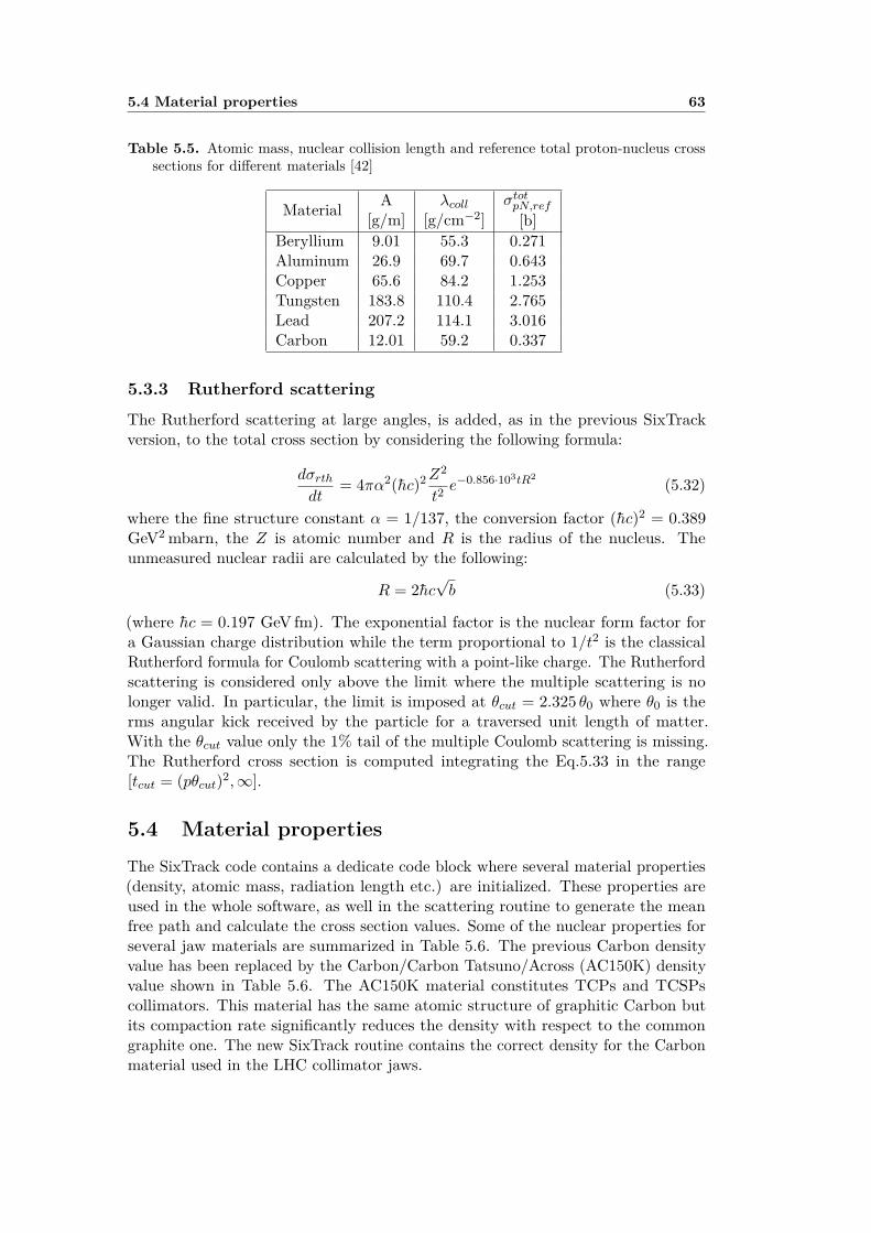
5.4 Material properties 63
Table 5.5. Atomic mass, nuclear collision length and reference total proton-nucleus crosssections for different materials [42]
Material A[g/m]
λcoll[g/cm−2]
σtotpN,ref[b]
Beryllium 9.01 55.3 0.271Aluminum 26.9 69.7 0.643Copper 65.6 84.2 1.253Tungsten 183.8 110.4 2.765Lead 207.2 114.1 3.016Carbon 12.01 59.2 0.337
5.3.3 Rutherford scattering
The Rutherford scattering at large angles, is added, as in the previous SixTrackversion, to the total cross section by considering the following formula:
dσrthdt
= 4πα2(hc)2Z2
t2e−0.856·103tR2 (5.32)
where the fine structure constant α = 1/137, the conversion factor (hc)2 = 0.389GeV2 mbarn, the Z is atomic number and R is the radius of the nucleus. Theunmeasured nuclear radii are calculated by the following:
R = 2hc√b (5.33)
(where hc = 0.197 GeV fm). The exponential factor is the nuclear form factor fora Gaussian charge distribution while the term proportional to 1/t2 is the classicalRutherford formula for Coulomb scattering with a point-like charge. The Rutherfordscattering is considered only above the limit where the multiple scattering is nolonger valid. In particular, the limit is imposed at θcut = 2.325 θ0 where θ0 is therms angular kick received by the particle for a traversed unit length of matter.With the θcut value only the 1% tail of the multiple Coulomb scattering is missing.The Rutherford cross section is computed integrating the Eq.5.33 in the range[tcut = (pθcut)2,∞].
5.4 Material propertiesThe SixTrack code contains a dedicate code block where several material properties(density, atomic mass, radiation length etc.) are initialized. These properties areused in the whole software, as well in the scattering routine to generate the meanfree path and calculate the cross section values. Some of the nuclear properties forseveral jaw materials are summarized in Table 5.6. The previous Carbon densityvalue has been replaced by the Carbon/Carbon Tatsuno/Across (AC150K) densityvalue shown in Table 5.6. The AC150K material constitutes TCPs and TCSPscollimators. This material has the same atomic structure of graphitic Carbon butits compaction rate significantly reduces the density with respect to the commongraphite one. The new SixTrack routine contains the correct density for the Carbonmaterial used in the LHC collimator jaws.

64 5. Improved physics model for SixTrack scattering routine
Table 5.6. Nuclear and atomic properties for implemented materials in SixTrack, inparticular atomic weight A, density ρ and radiation length χ0.
Material A ρ χ0[g mol−1] [g cm−3] [ m ]
Beryllium (Be) 9.01 1.848 0.353Aluminum (Al) 26.98 2.70 0.089Copper (Cu) 63.55 8.96 0.0143Tungsten (W) 183.85 19.3 0.0035Lead (Pb) 207.19 11.35 0.0056Carbon (C) 12.01 1.65 1 0.1881 New implemented AC150K density.
5.5 Detailed distribution of individual processes
As discussed above, when a charged particle passes through a thickness of materialundergoes continuos processes due to the electromagnetic interaction, such as multipleCoulomb scattering and ionization, and discrete processes due to the point-likeinteractions with the material nuclei. Each discrete process is characterized by afinite cross section related to its probability to occur and by a differential crosssection that gives the probability to find the scattered proton with a certain angleand momentum. After each simulated processes the interaction details, such as angleof the scattered proton, final proton energy, interaction length and interaction typeare recorded in a specific file called interactions_inside_jaw.dat.The angular distributions of the proton-proton single diffractive scattering, proton-proton elastic scattering and proton-nucleus elastic scattering are shown in Fig.5.14,Fig.5.15 and Fig.5.16 respectively. The simulations have been performed using thepencil beam configuration in the case of horizontal halo at 7TeV for Beam 1. Theselected collimator is the TCP.C6L7, made by AC150K material with a length of60 cm. In particular, all the impacting particles have the same energy and the sameangle x′ = 0 rad. From the plots is possible to observe that the major angular spreadis given by the single diffractive scattering.The single diffractive scattering is characterized by a not negligible particle momen-
Figure 5.14. Angular distribution of the proton-proton single diffractive scattering in xand y directions.

5.5 Detailed distribution of individual processes 65
Figure 5.15. Angular distribution of the proton-proton elastic scattering in x and ydirections.
Figure 5.16. Angular distribution of the proton-nucleus elastic scattering in x and ydirections.
tum transfer to the nucleus producing an new excited state of mass (see section5.3.1). The distribution of the energy variation with respect to the initial momentum,defined as: ∆E = pf − p0, is presented in Fig.5.17. The ionization contribution hasbeen subtracted from the final particle momentum. Most of the diffracted particleswere affected by an energy variation between 2GeV and 15GeV, while the variationenergy of the particles in the distribution tail reaches the 50GeV.
Figure 5.17. Energy variation of the scattered proton after p-p single diffractive process.


67
Chapter 6
Validation of the improvedscattering routine of SixTrack
The improvements in the scattering routine of SixTrack were described in detailed inthe previous Chapter. Detailed distributions of the outgoing angle and the changeof energy were shown for different interactions. However, the final validation of thecode has to be done in a more general way.In this chapter we investigate the change on the simulated distribution of the lossesalong the LHC ring after every change on the code. In particular we give especialemphasis at the change on the cleaning inefficiency in the dispersion suppressionregion of the IR7 and at the impacts at the TCTs in the IR1 and IR5.The previous SixTrack routine was validated agains the data with protons at 3.5 TeVbeam energy. Here we reproduce these results an give an update on the changesafter the improvements in the scattering routine.
6.1 Effect of scattering routine updates on simulations
In order to investigate the effect of each change in the SixTrack scattering routine,the losses in the dispersion suppression region of IR7 and the number of absorbedprotons at the collimators are studied for each individual change. The eight changesimplemented in the SixTrack scattering routine that are described in Chapter 5 are:
• case 0: This case corresponds to the previous SixTrack version.
• case 1: Update of the Carbon density that matches the Carbon used in thepresent collimation system.
• case 2: Case 1 with the update on the multiple coulomb scattering process,adding the logarithm part on the calculation of the angle rms.
• case 3: Case 2 with the implementation of the Bethe-Bloch equation tocalculate the energy loss by ionization.
• case 4: Case 3 with the update of the proton-proton elastic cross section,σelpp, including new data measurement from TOTEM Collaboration.

68 6. Validation of the improved scattering routine of SixTrack
• case 5: Case 4 with the updated of the proton-proton total cross section,σtotpp , including new data measurement from TOTEM Collaboration.
• case 6: Case 5 with the updated of the proton-proton single diffractive crosssection, σSDpp .
• case 7: Case 6 with the updated of the proton-nucleus total cross section,σtotpN , from the PDG.
• case 8: Case 7 with the updated of the proton-nucleus inelastic cross section,σinpN , from the PDG.
6.1.1 Simulation setup
In order to study the effect of the changes implemented in the scattering routine, thesimulations of protons at 7 TeV energy with LHC nominal settings before and afterthe changes are compared. For these simulations we used the collimator settingsshown in Fig. 6.1, expressed in beam sigma size with normalized transverse emittanceof 3.5 mm mrad. The beta-star at IP1 and IP5 was set to 0.55 m and to 10 m in IP2and IP8 as shown in Fig. 6.2.
Figure 6.1. Collimator settings for Beam 1 at 7 TeV, assuming normalized transverseemittance of 3.5 mm mrad.
Figure 6.2. Beta function at IP5 (same for IP1) and IP2 (same at IP8) for Beam 1, protonsat 7 TeV, nominal LHC optics.
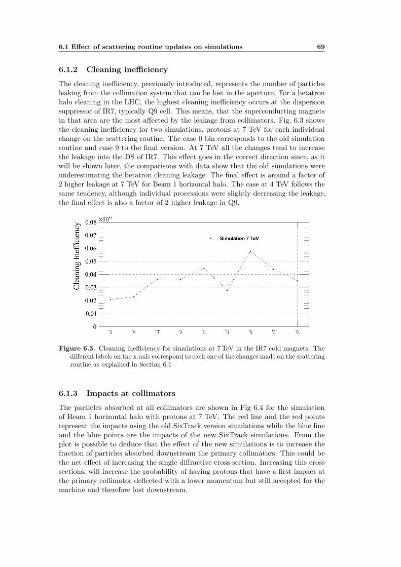
6.1 Effect of scattering routine updates on simulations 69
6.1.2 Cleaning inefficiency
The cleaning inefficiency, previously introduced, represents the number of particlesleaking from the collimation system that can be lost in the aperture. For a betatronhalo cleaning in the LHC, the highest cleaning inefficiency occurs at the dispersionsuppressor of IR7, typically Q9 cell. This means, that the superconducting magnetsin that area are the most affected by the leakage from collimators. Fig. 6.3 showsthe cleaning inefficiency for two simulations, protons at 7 TeV for each individualchange on the scattering routine. The case 0 bin corresponds to the old simulationroutine and case 9 to the final version. At 7 TeV all the changes tend to increasethe leakage into the DS of IR7. This effect goes in the correct direction since, as itwill be shown later, the comparisons with data show that the old simulations wereunderestimating the betatron cleaning leakage. The final effect is around a factor of2 higher leakage at 7 TeV for Beam 1 horizontal halo. The case at 4 TeV follows thesame tendency, although individual processions were slightly decreasing the leakage,the final effect is also a factor of 2 higher leakage in Q9.
Figure 6.3. Cleaning inefficiency for simulations at 7TeV in the IR7 cold magnets. Thedifferent labels on the x-axis correspond to each one of the changes made on the scatteringroutine as explained in Section 6.1
6.1.3 Impacts at collimators
The particles absorbed at all collimators are shown in Fig 6.4 for the simulationof Beam 1 horizontal halo with protons at 7 TeV. The red line and the red pointsrepresent the impacts using the old SixTrack version simulations while the blue lineand the blue points are the impacts of the new SixTrack simulations. From theplot is possible to deduce that the effect of the new simulations is to increase thefraction of particles absorbed downstream the primary collimators. This could bethe net effect of increasing the single diffractive cross section. Increasing this crosssections, will increase the probability of having protons that have a first impact atthe primary collimator deflected with a lower momentum but still accepted for themachine and therefore lost downstream.

70 6. Validation of the improved scattering routine of SixTrack
Figure 6.4. Particles absorbed at all collimators normalized to the particles absorbed atthe horizontal primary collimator in IR7.
6.2 Measurements of beam losses at the LHC
During LHC Run I (2010-2013), beam losses were generated periodically on dedicatedlow intensity fills in order to validate the collimation hierarchy settings and to identifythe limiting locations along the LHC ring. The beam was blown up independently invertical and horizontal plane until the beam tails touch the collimators, generatingbeam losses in all the collimation system.
6.2.1 Generation of beam losses: ADT and resonance method
To validate the collimation system, the beams are excited artificially in order togenerate sufficient loss rates to measure the collimation cleaning. Two methods havebeen used to blow up the beam and perform the loss maps: the Tune resonance (QT)and the Transverse Dumper (ADT) method. The resonance method is a techniqueto move the tune across a third order resonance in the vertical and horizontal plane.The excited beam in a plane can be affected by the tune changes in the other planecausing beam instability and uncontrolled losses in the machine. In most of the casesthe beam is dumped during the loss map measurements, for this reason a controlledtransverse blow up of the beam is required. The ADT method allows to performaperture measurements and loss maps with high intensity bunch trains without alimited bunch number needed. This technique was extensibly used during 2012 and2013 runs, and developed to blow-up transversely the LHC proton beams [43, 44].This method is based on white noise beam excitation in selected bunches, both inthe horizontal and the vertical plane independently. The speed of transverse blow-upcan be precisely controlled. This method is very precise and allows to control thelosses very accurately during the data taking. At the end of 2012 run it was possibleto excite individual 25 ns separated bunches without affecting the adjacent bunches.The ADT method was used for the collimation quench test in 2013 where losses upto 1MW were generated over few seconds in a very controlled way with unsafe beamintensity in the machine.

6.3 Validation of the SixTrack scattering routine with data 71
6.2.2 The BLM system
In order to protect the LHC superconducting magnets against quench and beaminduced damage, the losses are monitored mainly by the Beam Loss MonitoringSystem (BLM) that detects and quantifies the amount of lost beam particles. Itgenerates a beam abort trigger when the losses exceed predetermined thresholdvalues. The BLMs are ionization chambers to detect secondary particles originatingfrom the beam losses on the lattice elements: cold magnets, collimators, warmmagnets, etc. The detectors probe the transverse tails of the hadronic showersemerging from the cryostat, which are induced by lost beam particles. The voltageapplied to the electrodes of the ionization chamber moves the ionization chargesinducing a signal current on the two electrodes. In the ideal ionization chamberthe measured current is proportional to the amount of charges liberated by energydeposition from the passing particle. About 4000 detectors are installed, mostlyaround the quadrupole magnets, but also downstream each collimators, to controlthe beam losses and provide machine protection.
6.2.3 Loss maps during LHC Run I (2010-2013)
The local betatron cleaning inefficiency from 2010 to 2012 is shown in Fig 6.5 [45].The figure shows an excellent stability of the cleaning performance. The changesof cleaning inefficiency appears when the collimator settings were changed. In 2011the machine was running with the so-called relaxed collimators settings, while in2012 the so-called tight collimator settings (with reduce aperture) were used whichresulted on reducing the leakage in the DS of IR7.
18/06/1028/07/10
11/08/1027/08/10
04/10/1018/10/10
11/03/1104/04/11
12/04/11MD nominal
MD tight15/05/11
24/06/1113/07/11
05/09/1122/10/11
29/03/1231/03/12
02/04/1230/04/12
30/04/12MD nominal
MD nominal RC
01/07/1201/07/12
01/07/1211/07/12
16/07/1216/07/12
16/07/1223/11/12
23/11/12
Clea
ning
inef
ficie
ncy
-510
-410
-310
Relaxed Settings2010 3.5TeV
Relaxed Settings2011 3.5TeV
Tight Settings2012 4TeV
7 TeV design cleaning inefficiency
MD
nom
inal
MD
tigh
t
MD
nom
inal
B1 HORB1 VERB2 HORB2 VER
Figure 6.5. Collimation cleaning inefficiency as function of time since 2010 until end of2012 run [45].
Fig.6.6 shows a loss map of LHC during the Run I with the tight setting configuration.The distribution of the losses in the betatron cleaning insertion IR7 is also shown inFig.6.7.
6.3 Validation of the SixTrack scattering routine withdata
The ultimate validation of the SixTrack scattering routine should be done by com-paring the simulation predictions with the real measurements. This was done with

72 6. Validation of the improved scattering routine of SixTrack
s [m]0 5000 10000 15000 20000 25000
Loca
l cle
anin
g in
effic
ienc
y
-710
-610
-510
-410
-310
-210
-110
1
10coldcollimatorwarm
Noise in lossmeasurement
99.993% cleaning efficiency
IR1 IR1IR2
IR3
IR5
IR6
IR7
IR8
Figure 6.6. Distribution of the losses in the LHC ring [45].
s [m]19400 19600 19800 20000 20200 20400 20600
Loca
l cle
anin
g in
effic
ienc
y
-710
-610
-510
-410
-310
-210
-110
1
10
coldcollimatorwarm
Noise in lossmeasurement
cleaning efficiency99.993%
cleaning hierarchyIR7
Figure 6.7. Distribution of the losses in the betatron cleaning insertion IR7 [45].
the previous routine [46] by comparing the qualification loss maps with protons at3.5 TeV beam energy. Here we present the new comparison after the improvementson the scattering routine.
6.3.1 Machine configuration
This time the optics are configured to run with protons at 3.5 TeV beam energy. Thebeta-star in IP1 and IP5 was set to 1.5 m as shown in Fig.6.8. Fig. 6.9 shows thebeta-star configuration of IP2 (left) and IP8 (right). In this case, IP2 was configuredwith β? = 10 m while IP8 was configured with β? = 3 m.
6.3.2 Collimator settings
In 2011 the LHC machine was running with the so-called relaxed collimator settings.These settings are more relaxed, which means with more aperture than the nominalsettings but sufficient cleaning is still provided at the proton energy of 3.5 TeV.Table 6.1 and Fg.6.10 show the settings used for the simulations. The collimators
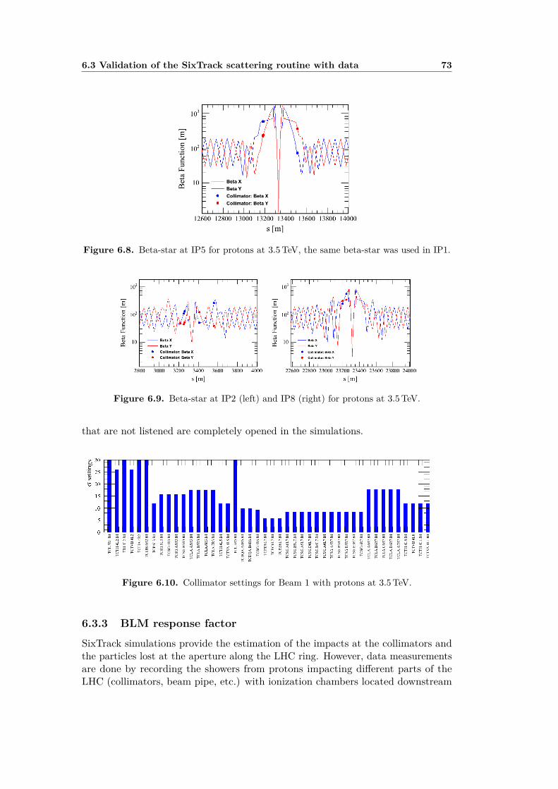
6.3 Validation of the SixTrack scattering routine with data 73
Figure 6.8. Beta-star at IP5 for protons at 3.5 TeV, the same beta-star was used in IP1.
Figure 6.9. Beta-star at IP2 (left) and IP8 (right) for protons at 3.5 TeV.
that are not listened are completely opened in the simulations.
Figure 6.10. Collimator settings for Beam 1 with protons at 3.5 TeV.
6.3.3 BLM response factor
SixTrack simulations provide the estimation of the impacts at the collimators andthe particles lost at the aperture along the LHC ring. However, data measurementsare done by recording the showers from protons impacting different parts of theLHC (collimators, beam pipe, etc.) with ionization chambers located downstream
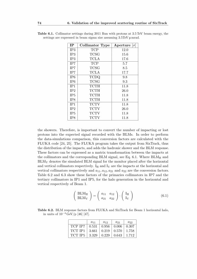
74 6. Validation of the improved scattering routine of SixTrack
Table 6.1. Collimator settings during 2011 Run with protons at 3.5 TeV beam energy, thesettings are expressed in beam sigma size assuming 3.5TeV µmrad.
IP Collimator Type Aperture [σ]IP3 TCP 12.0IP3 TCSG 15.6IP3 TCLA 17.6IP7 TCP 5.7IP7 TCSG 8.5IP7 TCLA 17.7IP6 TCDQ 9.8IP6 TCSG 9.3IP1 TCTH 11.8IP2 TCTH 26.0IP5 TCTH 11.8IP8 TCTH 11.8IP1 TCTV 11.8IP2 TCTV 26.0IP5 TCTV 11.8IP8 TCTV 11.8
the showers. Therefore, is important to convert the number of impacting or lostprotons into the expected signal recorded with the BLMs. In order to performthe data-simulations comparison, this conversion factors are calculated with theFLUKA code [24, 25]. The FLUKA program takes the output from SixTrack, thusthe distribution of the impacts, and adds the hadronic shower and the BLM response.These factors can be expressed as a matrix transformation between the impacts atthe collimators and the corresponding BLM signal, see Eq. 6.1. Where BLMH andBLMV denotes the simulated BLM signal for the monitor placed after the horizontaland vertical collimators respectively. IH and IV are the impacts at the horizontal andvertical collimators respectively and a11, a12, a21 and a22 are the conversion factors.Table 6.2 and 6.3 show these factors of the primaries collimators in IP7 and thetertiary collimators in IP1 and IP5, for the halo generation in the horizontal andvertical respectively of Beam 1.(
BLMHBLMV
)=(a11 a12a21 a22
)·(
IHIV
)(6.1)
Table 6.2. BLM response factors from FLUKA and SixTrack for Beam 1 horizontal halo,in units of 10−4 GeV/p [46] [47].
a11 a12 a21 a22TCP IP7 0.531 0.956 0.006 0.307TCT IP1 3.661 0.219 0.570 1.758TCT IP5 3.329 0.229 0.643 1.712

6.3 Validation of the SixTrack scattering routine with data 75
Table 6.3. BLM response factors from FLUKA and SixTrack for Beam 1 vertical halo, inunits of 10−4 GeV/p [46] [47].
a11 a12 a21 a22TCP IP7 0.531 0.956 0.006 0.307TCT IP1 3.824 0.210 0.604 1.723TCT IP5 3.569 0.281 0.781 1.637
6.3.4 Comparisons between data and simulations
The triplet quadrupole magnets are installed to reduce the optical β function in thecollision points of LHC. Tertiary collimators provide local beam cleaning to protectthe triplets avoiding magnet quenches.The TCTs intercept the the tertiary halo reducing the number of particle impactingon the superconducting triplet magnets. A comparison between measurements andsimulations of the impacts at the tertiary collimators are presented in Fig.6.11 at3.5TeV for Beam 1 horizontal halo case (top) and vertical halo case (bottom). Boththe measured and simulated losses are normalized to the number of particle lostat TCP collimators. The black line represents the BLM experimental data [46], inparticular the experimental points are the average ratio over all 2011 loss maps.The simulations have been performed for a perfect machine using the new SixTrackversion and the old SixTrack version: they are shown in the plot in blue and redrespectively. The dashed lines represent the simulation without FLUKA factorconversion while the solid lines represent the simulations after applying the BLMresponse factors calculated by FLUKA simulations [47].
Table 6.4. Maximum of losses on the cold magnets for the simulations with the newSixTrack version and the old SixTrack version (Beam 1 horizontal halo case).
Cold Magnet Max loss/(loss at TCP)New routine
Max loss/(loss at TCP)Old routine
Q8 3.073×10⁻⁵ 1.725×10⁻⁵
Q9 6.260×10⁻⁵ 3.558×10⁻⁵
Q10 7.967×10⁻⁶ 2.156×10⁻⁶
Q11 3.870×10⁻⁵ 1.833×10⁻⁵
Table 6.5. Integrated losses on the cold magnets for simulations with the new SixTrackversion and the old SixTrack version (Beam 1 horizontal halo case).
Cold Magnet Integrated loss/(loss at TCP)New routine
Integrated loss/(loss at TCP)Old routine
Q8 1.617×10⁻⁴ 8.217×10⁻⁴
Q9 4.454×10⁻³ 2.255×10⁻³
Q10 5.691×10⁻⁵ 1.617×10⁻⁵
Q11 3.910×10⁻³ 2.096×10⁻³
The FLUKA factors used in this analysis are shown in Table 6.2 and 6.3. Fromthe plot it is possible to appreciate an increase by a factor of ∼ 4 with respect to

76 6. Validation of the improved scattering routine of SixTrack
previous simulations producing a better estimation of the simulated losses comparedto experimental data. The complete simulated loss maps for Beam, horizontal halocase, at 3.5TeV are shown in Fig.6.12. The cleaning inefficiency on the y-axis hasbeen replaced by the ratio between the particles lost and the losses at the TCPcollimator. Fig.6.12a shows the losses in the complete ring simulated by using thenew version of the scattering routine, a zoom in the IR7 insertion is also shown inFig.6.12b.
(a) Beam 1 horizontal halo
(b) Beam 1 vertical halo
Figure 6.11. Losses at 3.5TeV from experimental data compared with the simulationsperformed with the new and old SixTrack version.

6.3 Validation of the SixTrack scattering routine with data 77
(a) Complete simulated loss map at 3.5TeV for Beam 1 horizontal (new SixTrack version).
(b) Zoom in IR7 of simulated loss map at 3.5TeV for Beam 1 horizontal (new SixTrackversion).
(c) Zoom in IR7 of simulated loss map at 3.5TeV for Beam 1 horizontal (old SixTrackversion).
Figure 6.12. Simulated loss map at 3.5TeV.
In addition the losses in the IR7 insertion simulated by using the old SixTrack versionare represented in Fig.6.12c. Considering the simulation with the new SixTrackversion, from the loss maps it is possible to notice an increase of the losses all aroundthe ring. Giving particular attention to the cold magnets located in IR7, Table 6.4gives the values of the maximum losses on the magnets for the new SixTrack versionand the previous one. In the case of the Q10 magnet is reached an increase by a

78 6. Validation of the improved scattering routine of SixTrack
factor of ∼ 4 compared to the previous routine simulations. Table 6.5 shows theintegrated losses for each cold magnets in IR7.The results of the 2011 comparison between measurements and simulation at theTCT collimators are presented in Fig.6.13 from [46] for Beam 1 horizontal halo andBeam 1 vertical halo. Both the measured and the simulated losses are normalizedto the number of particle lost at TCP collimators. The red line represents theBLM data, the green line are the simulations from SixTrack and the orange linerepresents the simulated impacting particles converted to the BLM signal using theFLUKA factors shown in Table 6.2 and 6.3 for Beam1 horizontal and vertical halorespectively. The plots are made by considering the machine with imperfections.The SixTrack simulation with a not perfect machine has been done by includingthe influence of random collimator imperfections such as error on tilt angles, beamcenter, gap and jaw curvature in IR7. A factor of 5 is obtained by comparing theperfect machine case in Fig.6.11 for the old SixTrack routine simulations with theimperfect machine case in Fig.6.13. From this comparison is possible to deduce thatapplying the new routine simulations to the imperfect machine case, a factor of 5from the imperfect case will bring the simulation predictions extremely close to thedata.
Figure 6.13. BLM signal ratio on horizontal and vertical TCTs to the TCPs in simulationswith machine imperfections and measurements in the 2011 machine [46].

79
Chapter 7
Improved estimation for 7TeVcleaning performance
The LHC has built to store, accelerate and provide particle collisions with a maxi-mum particle momentum of 7TeV with a nominal peak luminosity of L=1034 cm2 s−1.During the first run of the LHC with beam energies of 3.5TeV and 4.0TeV, no experi-ences of quenches induced by losses from circulating beams occurred. This situationmight change at 7TeV because of the reduced quench margin of the superconductingmagnets. Hence an excellent control of particle losses must be provided by thecollimation system. SixTrack simulations using the updated scattering routine havebeen performed to predict the cleaning performance at the designed energy of 7TeV.
7.1 Machine configuration at 7TeVThe LHC collimation system is designed to intercept beam losses and to absorbthem in the dedicated cleaning insertions in IR3 (momentum cleaning) and IR7(betratron cleaning). During the LS1 shutdown period the collimation system isbeing updated to provide adequate beam cleaning and machine protection at 7TeV.The nominal design collimator setting in IP3 and IP7 is presented in Table 7.1, theall collimator settings are presented in Table 3.3. The complete collimator layoutfor the nominal designed energy is shown in Fig.7.1, where in the y-axis are shownthe s-position in the LHC ring, the collimators settings used for all collimators areshown in Fig.7.2, where in y-axis are shown the half-gap positions in σ units.
Table 7.1. Collimator settings in IP3 and IP7 for the 7TeV machine configuration
7TeV Collimator setting [σ]IP3 IP7
TCP TCSG TCLA TCP TCSG TCLA15 18 20 6 7 10
During 2012 the LHC was operating at 4TeV with beta star at the ATLAS and theCMS interaction points of 0.6 m. The high luminosity insertions expects a betastar value at IP1 and IP5 of 0.55m. The collision optics at 7TeV in these twoinsertions are characterized by crossing angle of ± 142.5µrad. This scheme provides

80 7. Improved estimation for 7TeV cleaning performance
Figure 7.1. Collimator layout for Beam 1 at 7TeV proton energy.
Figure 7.2. Collimator settings at 7TeV proton energy.
an average beam-beam separation of 9.4σ. It is really important to keep a sufficientseparation between the two colliding beams to reduce any effects from long-rangebeam interaction. The main limit on the bunch intensity is indeed related to thebeam-beam effects. The IR2 insertion hosts the ALICE detector with β∗ = 10mfor protons and 0.5m for Pb ions. The transverse beam separation is 5σ. In IR8 isinstalled the LHCb experiment, here the collision optics expects a beta star of 10m.In IP2 and in IP8 the crossing angle are ± 150µrad and ± 200µrad respectively.The IR3 insertion hosts the Momentum Collimation system and provides momentumcleaning. Hence the collimators must be placed at locations with high dispersionand low betatron function, while the collimators in IR7 are placed at low dispersionfunction to provide betatron cleaning. The β-function in IR3 and in IR7 are shownin Fig.7.3, where the solid points indicate the β-function in a particular collimator.
Figure 7.3. β-function in IR3 (left) and IR7 (right) for Beam 1 using nominal LHC optics.

7.2 Loss maps at 7TeV 81
7.2 Loss maps at 7TeVThe better agreement between the experimental data and the updated SixTrackversion, shown in Chapter 6, leads to a better estimation of the losses around thering at 7TeV beam energy. In this section are presented the complete loss maps andthe detailed distributions of the losses at the betatron cleaning insertion (IR7), forBeam 1 and Beam 2, performed with the new SixTrack version. For Beam 2 thepositions of the machine elements (collimators, warm magnets, cold magnets, etc...)appear inverted because Beam 2 circulates in the opposite direction.
(a) Full ring
(b) Betatron cleaning insertion IR7
Figure 7.4. Simulated beam loss map at 7TeV with the new routine for Beam 1 horizontalhalo case.

827.
Improved
estimation
for7TeV
cleaningperform
ance
(a) Full ring
(b) Betatron cleaning insertion IR7
Figure 7.5. Simulated beam loss map at 7TeV with the new routine for Beam 1 vertical halo case.

7.2Loss
maps
at7TeV
83
(a) Full ring
(b) Betatron cleaning insertion IR7
Figure 7.6. Simulated beam loss map at 7TeV with the new routine for Beam 2 horizontal halo case.

847.
Improved
estimation
for7TeV
cleaningperform
ance
(a) Full ring
(b) Betatron cleaning insertion IR7
Figure 7.7. Simulated beam loss map at 7TeV with the new routine for Beam 2 vertical halo case.

7.3 Impacts at the primary collimators 85
7.3 Impacts at the primary collimators
Primary collimators are installed in the momentum cleaning insertion (IR3) and inthe betatron cleaning insertion (IR7). In IR3 the primary collimators are set with ahalf-gap of 15σ while in the IR7 they are set with a half-gap of 6σ.In the multi-stage collimation system the TCPs intercept the primary halo, generatedin this case at 6σ from the center of the beam orbit. Fig.7.8 shows the simulatedimpacts at primary collimators in IR7 with the new scattering routine, for Beam1 with a horizontal halo distribution, while Fig.7.9 shows the case of Beam 1 witha vertical halo distribution. The transverse distribution is presented with theprojections in x and y directions normalized to the collimator σ. The number ofparticles lost at the collimator are normalized to the collimator length and to thetotal number of particles absorbed at collimators. In Fig.7.10 and Fig.7.11 areshown the simulated impacts at the primary collimators in IR7 for Beam 2 with ahorizontal and a vertical halo distribution respectively.
(a) Horizontal TCP (b) Vertical TCP (c) Skew TCP
Figure 7.8. Transverse distribution projections of the impacts on the primary collimators,Beam 1 horizontal halo.
(a) Horizontal TCP (b) Vertical TCP (c) Skew TCP
Figure 7.9. Transverse distribution projections of the impacts on the primary collimators,Beam 1 vertical halo.

86 7. Improved estimation for 7TeV cleaning performance
(a) Horizontal TCP (b) Vertical TCP (c) Skew TCP
Figure 7.10. Transverse distribution projections of the impacts on the primary collimators,Beam 2 horizontal halo.
(a) Horizontal TCP (b) Vertical TCP (c) Skew TCP
Figure 7.11. Transverse distribution projections of the impacts on the primary collimators,Beam 2 vertical halo.
7.4 Losses at Dispersion Suppressor region at IR7
The dispersion suppressor (DS) region is a transition between the LHC arcs and theinsertions which aims to reduce the machine dispersion inside the insertions. Thedispersion suppressor regions are located at the end of each LHC arc and the tunnelgeometry determines their lengths. The critical locations for the LHC collimationsystem are the dispersion suppressors of cleaning insertions where dispersive lossesreach their maximum.The IR7 insertion contains the betatron cleaning system where the particles withlarge betratron amplitude in both vertical and horizontal directions are scatteredby the primary collimator jaws and absorbed by the secondary collimators. Thedispersion suppressor region in IR7 extends from Q8 to Q11 magnets, the protonswith a transverse amplitude large enough to impact on the vacuum chamber leavethe insertion and are lost on the machine apertures depositing energy on the machineequipments.Fig.7.12 shows the transverse distribution of the simulated impacts by using the newroutine in the ranges r1=20270-20350m (top) and r2=20370-20450m (bottom) ofthe the dispersion suppressor. The impacts are shown together with the projectionsin the x and y directions. The total number of particle lost in the cold magnetsnormalized by the total number of particles simulated is shown in Fig.7.13 for Beam1 horizontal halo case. The red line represents the simulations coming from the

7.4 Losses at Dispersion Suppressor region at IR7 87
Figure 7.12. Transverse distribution of the particle lost in the dispersion suppressor inIR7 for Beam 1 with horizontal halo distribution.
updated routine while the black line are the simulations of the previous SixTrackversion . The total number of particle lost in the cold magnets has been calculatedby integrating the histogram shown in Fig.7.12. With the new SixTrack version thelosses increase by about a factor of 2 in the first range r1 and by a factor of 1.5 inthe second range r2.A comparison at 7TeV of the number of particles lost at DS in IR7 between theupdated scattering routine and the old one is presented in Table 7.2 - 7.5 for Beam1 and Beam 2 with horizontal and vertical halo distributions. Table 7.2 - 7.5 showthe number of particle lost in each range with the ratio defined as the number oflost particles divided by the total number of particle generated.
Figure 7.13. Total of particle lost in the DS region at IR7 for Beam 1 horizontal halo case.

88 7. Improved estimation for 7TeV cleaning performance
Table 7.2. Beam losses and the ratio of the number of lost particles divided by the totalnumber of particle generated in the dispersion suppressor at IR7 Beam 1 horizontal halocase.
r1=20270-20350 r2=20370-20450Ratio Losses Ratio Losses
New Routine 2.26 × 10⁻⁴ 1078 1.95 × 10⁻⁴ 930Old Routine 1.08 × 10⁻⁴ 596 1.11× 10⁻⁴ 612
Table 7.3. Beam losses and the ratio of the number of lost particles divided by the totalnumber of particle generated in the dispersion suppressor at IR7 Beam 1 vertical halocase.
r1=20270-20350 r2=20370-20450Ratio Losses Ratio Losses
New Routine 2.31 × 10⁻⁴ 1477 2.36 × 10⁻⁴ 1509Old Routine 1.34 × 10⁻⁴ 857 1.48 × 10⁻⁴ 946
Table 7.4. Beam losses and the ratio of the number of lost particles divided by the totalnumber of particle generated in the dispersion suppressor at IR7 Beam 2 horizontal halocase.
r1=20270-20350 r2=20370-20450Ratio Losses Ratio Losses
New Routine 4.22 × 10⁻⁴ 2698 2.11 × 10⁻⁴ 1349Old Routine 2.61 × 10⁻⁴ 1668 1.38× 10⁻⁴ 882
Table 7.5. Beam losses and the ratio of the number of lost particles divided by the totalnumber of particle generated in the dispersion suppressor at IR7 Beam 2 vertical halocase.
r1=20270-20350 r2=20370-20450Ratio Losses Ratio Losses
New Routine 2.95 × 10⁻⁴ 1886 1.95 × 10⁻⁴ 1247Old Routine 1.77 × 10⁻⁴ 1131 1.20× 10⁻⁴ 767
With the new routine the losses increase from a factor of 1.5 to a factor of 2 comparedto the simulated losses with the old SixTrack version.
7.5 Impacts on TCTs
Collisions at√s = 14TeV require a high efficiency collimator system due to the
maximal energy deposition and local aperture restrictions at the experimental triplets.The triplets consist in three quadruple magnets installed to reduce the optical βfunction at the IPs. In order to protect the triplet magnets local beam cleaningis provided by the tertiary collimators (TCTs). The tertiary collimators interceptand dilute the tertiary halo, avoiding quenches because of the less impacting energyon the superconducting triplet magnets. The number of particles absorbed by the

7.6 Parametric study for 7TeV simulations 89
tertiary collimators are shown in Fig.7.14 for B1 horizontal halo case. The blueline represents the simulation performed with the new version of the scatteringroutine, while the red line represents the simulations performed with the old one.The number of expected impacts increase by a factor of ∼2 for the new routinewith respect to the old one. In both cases, new and old simulations, the numberof particles absorbed by the TCTs in IR2 is below 10−7. The increase of particleabsorbed is expected from the data comparison since the new version simulationsget closer to the experimental data by about a factor of 2 with respect to the oldroutine. In particular, the behavior for both versions is the same except for thetertiary collimators at IP8. In this case the previous version shows more impactson the tertiary collimators by a factor of ∼4 with respect to the new one for thehorizontal TCT collimator. Moreover no hit affects the vertical tertiary collimatorin IP8 in the case of the previous routine while few impacts can be observed withthe simulations carried out with the updated SixTrack routine, however the errorsin these points are larger due to the lack of statistics.
Figure 7.14. Number of particles absorbed in TCT collimators with new scattering routine(blue) and the previous one (red) normalized to the total particles absorbed in thecollimation system.
7.6 Parametric study for 7TeV simulations
A parametric study varying the proton-proton single diffractive cross section andthe proton-proton elastic cross section values was carried out by using the updatedscattering routine for 7TeV simulations. This study allows to understand how theuncertainty on the cross sections affects the cleaning performance and the impactson the tertiary collimators. The proton-proton single diffractive cross section wasmodified by a fixed amount of ±20% and ±50%, the proton-proton elastic crosssection was modified by a fixed amount of ±20%. The effects produced on the

90 7. Improved estimation for 7TeV cleaning performance
cleaning inefficiency by the single diffractive cross section variation are presented inTable 7.6 and in Table 7.7 for Beam 1 horizontal halo case.
Table 7.6. Maximum cleaning inefficiency on the cold magnets in IR7 for ± 20% variationof single diffractive cross section.
Cleaning Inefficiency×10−5 [1/m]σSD -20% New simulation σSD +20%
Q8 1.151 1.104 1.481Q9 2.796 3.532 5.595Q10 0.164 0.221 0.329Q11 1.480 2.428 3.291
Table 7.7. Maximum cleaning inefficiency on the cold magnets in IR7 for ± 50% variationof single diffractive cross section.
Cleaning Inefficiency×10−5 [1/m]σSD -50% New simulation σSD +50%
Q8 0.822 1.104 2.200Q9 1.316 3.532 4.716Q10 0.164 0.221 0.314Q11 1.809 2.428 5.659
Table 7.8. Maximum cleaning inefficiency on the cold magnets in IR7 for ± 20% variationof proton-proton elastic cross section.
Cleaning Inefficiency×10−5 [1/m]σel -20% New simulation σel +20%
Q8 1.151 1.104 0.986Q9 5.589 3.532 3.945
Q10 0.329 0.221 0.329Q11 4.767 2.428 2.794
In particular, the maximum cleaning inefficiency is given for the cold magnets inIR7: Q8, Q9, Q10 and Q11. In the case of Q8 magnet the variation of -20% doesnot produce relevant difference with respect to the case without variation,The maximum variation of the cleaning inefficiency in the case of -20% of the proton-proton single diffractive cross section is about a factor of 0.6 for the Q11 magnet. Inthe case of +20% of the proton-proton single diffractive cross section the maximumvariation of the cleaning inefficiency reaches a factor of 1.6 for the Q9 magnet. Thevariation of -50% of the single diffractive cross section produces a maximum cleaninginefficiency variation by a factor ∼ 0.4 in the case of Q9 magnet, while in the case ofa variation of +50% the maximum cleaning inefficiency reaches a factor of 2.3 forthe Q11 magnet. Table 7.8 shows the effects on the cleaning inefficiency produced bythe proton-proton elastic cross section variation. In this case a maximum cleaninginefficiency variation by a factor of 1.6 is reached in the case of Q9 magnet for avariation of the proton-proton elastic cross section of -20%. The variation of +20%

7.6 Parametric study for 7TeV simulations 91
Figure 7.15. Effects on the impacts at TCT collimators in IR1 and IR5 for a σSDpp ± 20%
variation and a σSDpp ± 50% variation, Beam 1 with a horizontal halo distribution.
of the same cross section produces a maximum cleaning inefficiency increase by afactor of ∼ 1.5 in the case of Q10 and Q11 magnets.The effects on the simulated impacts with the new SixTrack version at TCT colli-mators in IR1 and IR5 are presented in Fig.7.15. The yellow band represents theimpacts at the TCTs with a ±20% variation of the single diffractive cross section, theorange band represents the impacts with a ±50% variation of the single diffractivecross section and the black points are the simulated impacts for the case withoutvariation. The impacts are normalized to the total number of particles absorbed bythe collimators. For the ±20% variation of the single diffractive cross section, themajor impact difference can be appreciated on the tertiary collimators TCTH.4L5and TCTVA.4L5 at IR5. In particular, for TCTH.4L5 collimator the +20% variationof the single diffractive cross section moves up the impacts level about 8% of relativedifference, while the -20% variation results into a decrease about 14% of relativedifference with respect to the case without variation. For the TCTVA.4L5 collimatorthe +20% variation of the single diffractive cross section moves up the impacts about6% of relative difference with respect to the reference case without variation, whilethe -20% variation of the single diffractive cross section increases the impacts with arelative difference of ∼ 21%. For the ±50% variation of the single diffractive crosssection, the major impact difference can be appreciated on the tertiary collimatorsTCTH.4L5 at IR5 and TCTVA.4L1 at IR1. In the case of the TCTH.4L5 collimator,the +50% variation produces an increase of the impacts with a relative differenceabout 9%, while the -50% variation results into a decrease about 31% of relativedifference with respect to the case without variation. For the TCTVA.4L1 collimator,the +50% variation of the single diffractive cross section moves down the impactslevel about 15% of relative difference, while the -50% variation results into an increaseabout 20% of relative difference with respect to the reference case.The proton-proton elastic cross section was also varied by ±20%, however no signifi-cant changes in the number of impacts at the TCTs was found.


93
Chapter 8
Conclusions
The LHC machine is designed to accelerate two proton counterrotating beams, up to7TeV, that collides in the experimental detectors. Also ions (Pb) can be acceleratedup to 574TeV per nucleus. Due to the high beam intensity the energy depositionof the beam losses around the machine must be always monitored and kept undercontrol. An energy deposition of about 5 mJ s−1 cm−3 is indeed enough to quenchthe LHC superconducting magnets cooled to a temperature between 1.8 K and 4.5K. To prevent dangerous beam losses an efficient collimation system is of crucialimportance. The collimator system provides beam cleaning, guarantees a smoothand safe operation of the machine and reduces the background for the experiments.Collimation studies aim to limit the number of particles that escape from thecollimator insertions and keep under control the beam losses. The collimationstudies are carried out also by means of simulations using the SixTrack software.This is a complex program able to track a large number of halo particles element-by-element using transfer matrices to describe the effect of each lattice element. Theinteraction of the protons with the collimator jaws is implemented in a dedicatedscattering routine based on a Monte Carlo method. The scattering routine simulatesthe nuclear and the electromagnetic processes between protons and the collimatormaterial nuclei. The scattering routine originates from the K2 code developed duringthe 1990’s and afterwards integrated in the SixTrack source code. An update of thisroutine by using new recent experimental data was necessary to better describe theinteraction processes at higher energy. In order to introduce effective modificationsable to provide a better approximation of the experimental data a deep investigationon the physics model underlying the scattering routine has been carried out. Asresult of this study several changes have been considered and then implemented inthe scattering routine regarding both the electromagnetic and nuclear processes:
• A different Carbon density that better fits the real collimator jaw material hasbeen included in the routine.
• The logarithmic term in the in the rms angle equation of the multiple Coulombscattering has been added. In the old scattering routine this term was missing.This logarithmic correction gave a larger spread of the protons outside of thecollimator.
• To better estimate the ionization losses the Bethe-Bloch equation has been

94 8. Conclusions
implemented in the routine. In the previous routine version the energy loss byionization was described by a constant term for any given energy.
• To better extrapolate the proton-proton elastic and total cross sections newfits were computed and included on the basis of recent measurements from theTOTEM collaboration.
• The proton-proton single diffractive cross section has been updated consideringa recent parametrization based on the renormalized pomeron flux exchange.
• The proton-nucleus inelastic and total cross sections have been updated con-sidering the new available data from the Particle Data Group.
The overall effect is an increase of the impacts downstream the collimator system.This trend is mainly due to the increase of the single diffractive cross section withrespect to the previous parametrization. The validation of the updates made waspresented in the Chapter 6, where the result of the comparison with data at 3.5TeVis presented. The simulations performed with the updated version of the scatteringroutine show, as general trend, an outcome closer to the experimental data by a factor∼3, for Beam 1 horizontal halo case and by a factor ∼2 for Beam 1 vertical halo case,with respect to the previous routine version simulations. On the basis of the presentedcomparisons with the previous routine version, validated by a clear reduction of thespread with experimental data, it is possible to state that the modifications appliedto the scattering routine resulted into a significative improvement in the simulationof the nuclear and the electromagnetic processes between protons and the collimatorjaw material.The LHC design energy of 7 TeV for each beam has been not achieved yet, themaximum level achieved was reached in March 2013 with 4TeV energy beams.Because of the quench limit decrease at higher energy, the requirements for thecollimation system performance will be more demanding than to the ones addressedin previous run. Therefore, the prediction of the cleaning inefficiency at higherenergies is under investigation. In Chapter 7 the simulations results at 7TeV arepresented, these simulations were performed with the improved scattering routine.The expected number of particles lost on the tertiary collimators, that protectthe triplet magnets in the collision points, increases by a factor 2 with respect tothe previous simulations results. Furthermore, the increase factor of the predictedleakage at the cold magnets in the Dispersion suppression in IR7 varies between afactor of 1.5 and a factor of 2.At 7TeV, the proton-proton single diffractive cross section was varied by ±20% and±50% in order to determine the uncertainty on the cleaning inefficiency. This studyindicates that the cleaning inefficiency in the Dispersion Suppressor region can varyin a range from 0.6 to a factor of 1.6 for a change of ±20% of the single diffractivecross section, and in a range from 0.4 to a factor of 2.3 for a ±50% variation of thiscross section.As a follow up of this work, further simulations using the new scattering routine willbe performed in order to provide:
• a quantitative comparison between 3.5TeV experimental data and imperfectmachine simulations. The imperfect machine case applied to the old routine

95
simulations increases the simulated losses at the tertiary collimators in IP1and IP5 by a factor of ∼5 (see Fig.6.13 from [46]). Similarly, a furtheragreement is expected between the losses predicted with the new routine andthe experimental data;
• future comparisons between simulations and 7TeV experimental data whenthe design beam energy will be reached to confirm the new routine simulationresults at this energy level.
In order to provide a more detailed picture of the ionization losses at higher energy:
• the tail contribution of the ionization energy loss distribution may also beconsidered in the scattering routine;
• the radiation losses for high energy protons can be included in the calculationof the Bethe-Bloch equation.
Those research paths can result in further improvements in the scattering routinesimulation capability.


97
Bibliography
[1] M. Martini. An introduction to transverse beam dynamics in accelerators.CERN/PS 96-11, 1996.
[2] H. Wiedermann. Particle Accelerator Physics. Springer, 3rd edition, 2007.
[3] K. Wille. The Physics of Particle Accelerators, an introduction. OXFORDUniversity Press, first edition, 1996.
[4] G. Robert-Demolaize. Design and Performance Optimization of the LHCCollimation System. PhD thesis, Universite Joseph Fourier, Grenoble, 2006.
[5] C. Bracco. Commissioning Scenarios and Tests for the LHC Collimation systemResistive transition and protection of LHC superconducting cables and magnets.PhD thesis, EPFL Lausanne, 2008.
[6] A. Piwinski. The touschek effect in strong focussing rings. DESY 98-179, 1998.
[7] M. Sands. The physics of electron storage rings. SLAC report 121, 1970.
[8] http://lhc-collimation-project.web.cern.ch/.
[9] M.Tigner A.Wu Chao. Accelerator physics and engineering. World ScientificPublishing, 1st edition, 1999.
[10] Cern - the large hadron collider. http://home.web.cern.ch/about/accelerators/large-hadron-collider.
[11] M. Benedikt, P. Collier, V. Mertens, J. Poole, and K. Schindl (editors). LHCdesign report v.3 : The LHC injector chain. CERN-2004-003-V3, 2004.
[12] https://espace.cern.ch/liu-project/LIU_images/Forms/DispForm.aspx?ID=11.
[13] O. S. Brüning, P. Collier, P. Lebrun, S. Myers, R. Ostojic, J. Poole, andP. Proudlock (editors). LHC design report v.1 : The LHC main ring. CERN-2004-003-V1, 2004.
[14] ATLAS Collaboration. The ATLAS experiment at the CERN Large HadronCollider. JINST, (3):S08003, 2008.
[15] CMS Collaboration. The CMS experiment at the CERN LHC. JINST,(3):S08004, 2008.

98 Bibliography
[16] LHCb technical proposal. CERN/LHCC 98-4, LHCC/P4, 1998.
[17] ALICE Collaboration: F. Carminati, P Foka, P Giubellino, A Morsch, G Paic,J-P Revol, K Safarik, Y Schutz, and U. A. Wiedemann (editors). Alice: Physicsperformance report, volume i. Journal of Physics G: Nuclear and ParticlePhysics, 30(11):1517–1763, 2004.
[18] http://cerncourier.com/cws/article/cern/54384.
[19] F. Schmidt. SixTrack. User’s Reference Manual. CERN/SL/94-56-AP, 1994.
[20] G. Robert-Demolaize, R. Assmann, S. Redaelli, and F. Schmidt. A new versionof sixtrack with collimation and aperture interface. Proc. of the ParticleAccelerator Conf. 2005, Knoxville, page 4084, 2005.
[21] T. Trenkler and J.B. Jeanneret. K2, a software package evaluating collimationsystems in circular colliders (manual). CERN SL/94105 (AP), 1994.
[22] http://mad.web.cern.ch/mad/.
[23] S. Redaelli, R. Assmann, and G. Robert-Demolaize. Lhc aperture and commis-sioning of the collimation system. Proceedings of the LHC Project WorkshopChamonix XIV, 2005.
[24] A. Fasso et al. CERN-2005-10, 2005.
[25] A. Fasso and others. The physics models of FLUKA: status and recent devel-opments. Proc. of the Computing in High Energy and Nuclear Physics 2003Conf., La Jolla, 2003.
[26] G. Battistoni, S. Muraro, P. R. Sala, F. Cerutti, A. Ferrari, S. Roesler, A. Fasso,and J. Ranft. The fluka code: Description and benchmarking. Hadronic ShowerSimulation Workshop 2006, Fermilab 6–8 September 2006, AIP ConferenceProceeding, 896:31–49, 2007.
[27] Passage of particles through matter. The Review of Particle Physics: 2005Reviews Tables and Plots, Particle Data Group web page "http://www.test.org/doe/".
[28] P.G.Rancoita C.Leroy. Radiation interaction in matter and detection. WorldScietific, 2004.
[29] W.R.Leo. Techniques for nuclear and particle physics experiments. Springer-Verlag, 2nd edition, 1994.
[30] H.A.Bethe. Moliere’s theory of multiple scattering. Phys. Rev., 89(6):1256, Mar1953.
[31] N.Catalan Lasheras. Collimacion transversal y longitudinal de un haz theprotones de alta energia an el Gran Colisionador de Hadrones (LHC). PhDthesis, Universidad de Zaragoza, 1998.
Bibliography 99
[32] K.Greisen B.Rossi. Cosmic-ray theory. Review of Modern Physics, 13(4):240.
[33] G.bellettini et al. Proton-nuclei cross sections at 20 gev. Nuclear Physics,79(3):609–624, May 1966.
[34] G. Antchev et al. Luminosity-independent measurement of the proton-protontotal cross section at
√s = 8 Tev. Physical Review Letter, 111(1):9, Jul 2013.
[35] The TOTEM Collaboration et al. Measurement of proton-proton elastic scat-tering and total cross-section at
√s = 7Tev. Europhysics Letters, 101(2):21002,
Jan 2013.
[36] K. Goulianos. Diffractive interactions of hadrons at high energies. PhysicsReports vol. 101, pp. 171-219, 1983.
[37] D. Bernard and the UA4 Collaboration. Physics Letters B, 186:227, 1987.
[38] D.Bernard and the UA4 Collaboration. Measurament of small angle antiproton-proton elastic scattering at
√s=546 and 1800 gev. Physics Review D, 50:5518,
1994.
[39] N.A. Amos, others, and E710 Collaboration. Physics Letters B, 301:313, 1993.
[40] K.Goulianos. Renormalization of hadronic diffraction and the structure of thepomeron. Physics Letters B, 358:379–388, 1995.
[41] A. Schiz et al. Hadron-nucleus elastic scattering at 70, 125 and 175 gev/c.Physical Review D, 21(11):3010–3022, 1980.
[42] Particle data group-atomic nuclear properties. http://pdg.lbl.gov/2013/AtomicNuclearProperties/index.html.
[43] W.Höfle, R.Assmann, S.Redaelli, R.Schmidt, D.Valuch, D.Wollmann, andM.Zerlauth. Controlled transverse blow-up of high- energy proton beams foraperture measurements and loss maps. CERN-ATS, 128.
[44] W.Höfle, F. Dubouchet, G. Kotzian, and D. Valuch. Performance of the lhctransverse damper with bunch trains. CERN-ACC, 0216.
[45] B. Salvachua et al. Cleaning performance of the lhc collimation system up to4Tev. CERN-ACC-2013-0070, 2013.
[46] R.Bruce et al. Simulations and measurements of cleaning with 100 MJ beamsin the LHC. CERN-ACC-2013-0113, 2013.
[47] E. Skordis and R. Bruce. FLUKA simulations of BLM response. LHC Collima-tion working group (6/5/2013).
