AN IMPLEMENTATION OF THE PLANNING PHASE OF TRIANA USING THE FLEXIBLEPOWER APPLICATION INFRASTRUCTURE

by

STERGIOS DAGIOGLOU

A THESIS

submitted in partial fulfillment of the requirements for the degree of

Master of Science

SUSTAINABLE ENERGY TECHNOLOGY

Faculty of Engineering Technology(Construerende Technische Wetenschappen - CTW)

UNIVERSITY OF TWENTEThe Netherlands

August 2014

to my family

Acknowledgments

This thesis was conducted in the period September 2013 - August 2014, partially at the University ofTwente (Faculty of Electrical Engineering, Mathematics and Computer Science, Departments of ComputerScience and Applied Mathematics) and partially during the internship conducted in the period 3 February-2 May 2014 at the facilities of TNO located in Groningen, the Netherlands and within the department ofBusiness Information Services − BIS. I would like to thank my supervisors at the University of Twente,Professor Johann Hurink and Ph.D. candidate Hermen Toersche as well as my supervisors at TNO,Wilco Wijbrandi and Dennis Krukkert for their valuable advice and guidance while carrying out thisassignment.

Abstract

Over the last decades, the impacts induced from human activities on the planet are a multiple of theimpacts the human species induced since its existence. The technological advancements of the first andsecond Industrial Revolution, led to a rapid growth of world population and life expectancy and to asubsequent growth of world energy consumption. Human technology is still improving very fast andpredictions show that world population and energy consumption will further increase over the comingdecades. Although all these technological advancements improved the quality of life for a large part ofthe world population, they also had tremendous impacts on the environment that threaten the ability offuture generations to meet their own needs. The greenhouse effect, deforestation, drought and potablewater shortage, biodiversity loss, are only some of the problems that the future generation will inherit asa result of the human activity of the last centuries.

The energy used to produce the electricity consumed nowadays, is approximately one third of the energyconsumed world-wide. But only less of the half of the energy used to produce electricity is finally convertedto electricity, as a result of the losses that occur during the production of electricity [34]. After electricityis produced 5-10 % of this energy is lost during the transmission and distribution of electricity to theend-users [2]. The largest part of the electricity consumed today, is still produced by large power plantsusing fossil fuels like coal and oil and is delivered to the consumers using the transmission and distributiongrids that result in the losses mentioned above. The efficiency of these power plants is also relatively lowunless used for the parallel production of heat and electricity (Combined Heat and Power-CHP).

The aforementioned evolutions lead governments and other administrative institutions to the establish-ment of measures that protect the environment and improve the overall energy production chain. Anexample is the “20-20-20” target of the European Union that aim to 3 objectives by 2020: reducing theEU greenhouse emissions by 20% compared to 1990, produce 20% of the energy consumed using renewablesources and improve energy efficiency by 20% [28].

As far as electricity is concerned, the evolution of the above grid to a Smart Grid is considered a necessityin order to achieve goals like the ones mentioned. Although it is risky to give an explicit definition ofthe Smart Grid, we could generally argue that the Smart Grids are systems which use modern tech-nologies to create more efficient energy systems compared to the present ones. A Smart Grid usuallycombines decentralized energy production (often from renewable energy sources), smart metering, infor-mation technology, energy storage devices, load and generation monitoring and control and other moderntechnologies to produce and distribute electrical and thermal energy in the most efficient way possible [12].

Some of the challenges the electric utilities face today are meeting the rising electricity demand with-out a parallel increase in greenhouse emissions, improving the efficiency with which energy is produced,transmitted and distributed and increasing the grid reliability so that an uninterrupted energy supplycan be made possible to a larger extent. Regarding the latter one, the electricity supply is frequentlythreatened during the hours of peak electricity consumption. Utilities must always be prepared to meetthe maximum electricity consumption expected. An interrupted or disturbed (regarding the voltage andfrequency levels) electricity supply has major negative effects on industries whose operation depends on astable electricity supply but also to commercial consumers as electricity is necessary to meet basic needsnowadays. Furthermore, meeting the large peak demands have a negative financial impact to electricityproducers as they can use cheaper energy sources to cover the base and intermediate demand and have touse more expensive sources to cover the peak demand. One method to reduce the peak electricity demandis to shift demand from peak hours to hours with lower demand. By this the need for expensive peakproduction units is decreased as well as the cost of the electricity production. Till now the production

1

was driven by the demand of consumers. Demand Side Management (DSM) technology is one the SmartGrid aspects and aims to shift the energy consumption from hours of high consumption to hours of lowerconsumption. By doing so, the electricity production can in a certain extent reduce its dependence onthe electricity demand. That would allow the energy producers to use cheap sources to cover a largerpercentage of the electricity consumed and increase the grid reliability. DSM and the improvements inforecasting the electricity produced by renewable sources may also lead to a larger integration of electricityproduced by renewable energy sources.

DSM usually includes an application which can communicate with the devices whose energy consumptionis desired to be controlled. An important problem that holds up the implementation of DSM in largescale is that devices use different communication protocols to send messages or data to other devices orcontrollers making the communication between devices and energy applications difficult. The FlexiblePower Application Infrastructure (FPAI) is a platform developed by the Netherlands Organisation forApplied Scientific Research (TNO) which aims to solve this problem. The purpose of FPAI is to createan intermediate platform that is able to connect to a variety of devices and also to support differentDSM systems [24]. Furthermore if a user wants to substitute its current DSM system with another,nowadays the installation of a new device that contains the hardware and software of the new systemwould be necessary. With FPAI the user just needs to uninstall the previous system and install a new one.

One of the many DSM methodologies developed during the last years is Triana; a DSM technique devel-oped at the University of Twente. The goal of the Triana methodology is given in [4] and it is “to managethe energy profiles of individual devices in buildings to support the transition towards an energy supplychain which can provide all the required energy in a sustainable way”. Triana has three main stages:Forecasting, Planning and Real-time Control. The ultimate goal of Triana is to exploit the flexibility ofdevices in order to achieve a goal related to the energy consumption of these devices. A typical goal is toachieve an aggregated energy consumption profile for a number of devices that is as flat as possible. Inthe Forecasting step, Triana tries to predict the flexibility offered by devices for a specific time horizon.Flexibility denotes the range of controllability of every device; how much the consumption pattern of adevice can be altered in order to achieve a certain goal for a number of devices. The flexibility of devicescan be estimated by determining parameters that influence the operation of a device. For example a usefulparameter for a domestic device that consumes electricity and produces heat, would be to predict theheat demand of the house (using information like weather data). The Planning phase takes into accountthe flexibility of a number of devices and determines the operation of devices for a planning horizon, inorder to achieve a global goal. In Real-time Control a replanning process might need to take place if wefind that the forecast which formed the base for the Planning did not lead to the desired goal. Hereby,the replanning process takes into consideration new forecasts which use more recent data related to thebehavior of the devices.

The research question of the current thesis is to explore if it is possible to implement the Planning phaseof Triana using the FPAI platform. It was considered useful for both the developers of FPAI and Trianato search if FPAI can indeed provide a platform on top of which Triana can be executed, as FPAI hadpreviously been used by only one other DSM system, the Powermatcher. During the implementation,incompatibilities between FPAI and Triana had to be detected and by using specific tools provided byFPAI or by introducing additional methods the gap between FPAI and Triana had to be bridged.

In order to answer this research question, a software programme has been implemented that executes thePlanning of Triana on top of FPAI. Using this software, a number of simulations was done to examine ifthe Planning results were the desired, thereby proving that the implementation of the Planning phase ofTriana using FPAI is indeed possible.

2

This thesis contains material that was written during a literature research that was done as a preparationof the thesis as well as material from the internship that was conducted in TNO facilities at Groningenand includes the development of the software that executes the Planning phase of Triana using the FPAI.

The first chapter of the thesis describes the relation of the topic of the thesis with the master programmeof Sustainable Energy Technology. The reader can find there information about how this topic is relatedto the aspects of sustainability. The second chapter describes in more detail the Triana methodology. Thethree steps of Triana are discussed in detail. It also includes information about the Powermatcher systemand a brief description of other energy control methodologies. The largest part of this chapter was writ-ten within the literature research which was made as a preparation assignment for the thesis. The thirdchapter contains a description of FPAI where we focus mainly on the aspects of FPAI which are neededfor the implementation of this assignment. The fourth chapter presents in detail how the implementationof the Planning phase of Triana using FPAI was done; how certain tools provided by FPAI were used, theincompatibilities between FPAI and Triana and how they were overcome and the specific implementationfor the different device types within FPAI. The fifth chapter presents the results of the simulations thatwere run to see if the code developed produced the results that were expected, namely if certain goalsrelated to the energy behavior for a number of devices were achieved using Triana. Finally in the sixthchapter we present our conclusions about the results of this thesis and recommendations for future workthat can be done.

3

Acronyms

CHP Combined Heat and PowerCOP Coefficient of Performance

DP Dynamic ProgrammingDSM Demand Side Management

ECN Energy research Center of the Netherlands

FAN Flexiblepower Alliance NetworkFIT Feed In TariffFP Flexible PowerFPAI Flexible Power Application Infrastructure

ICT Information and Communication TechnologyIDDP Iterative Distributed Dynamic Programming

MAS Multi-Agent System

PHEV Plug-in Hybrid Electric Vehicle

RAI Resource Abstraction InterfaceRAL Resource Abstraction Layer

SDM Supply-Demand MatchingSoC State of Charge

TOU Time of Use

VPP Virtual Power Plant

WSN Wireless Sensor Networks

4

List of Figures

1 World energy consumption by year . . . . . . . . . . . . . . . . . . . . . . . . . . . . . . . 102 World population by year . . . . . . . . . . . . . . . . . . . . . . . . . . . . . . . . . . . . 103 CO2 in atmosphere by year and average global temperature by year [1], [15] . . . . . . . . 114 The three dimensions of sustainability . . . . . . . . . . . . . . . . . . . . . . . . . . . . . 145 CO2 Emissions from Fuel Combustion (2012), Source: International Energy Agency . . . 156 Daily demand curve: DSM technologies aim at shifting the consumption from peak hours

to hours of lower consumption . . . . . . . . . . . . . . . . . . . . . . . . . . . . . . . . . 167 The tree structure of Triana . . . . . . . . . . . . . . . . . . . . . . . . . . . . . . . . . . . 188 Real and predicted heat demand values [4] . . . . . . . . . . . . . . . . . . . . . . . . . . . 219 The mismatch of the planning when the same (solid line) of different (dashed line) price

vectors are used in the simulation of 50 houses [4] . . . . . . . . . . . . . . . . . . . . . . . 2210 Mismatch in the second simulation is less when different price vectors are steered to each

house controller [4] . . . . . . . . . . . . . . . . . . . . . . . . . . . . . . . . . . . . . . . . 2311 The cost of importing or exporting electricity is linear to amount of energy imported or

exported [4] . . . . . . . . . . . . . . . . . . . . . . . . . . . . . . . . . . . . . . . . . . . . 2412 The results of the second use case [4] . . . . . . . . . . . . . . . . . . . . . . . . . . . . . . 2613 The results of the third case [4] . . . . . . . . . . . . . . . . . . . . . . . . . . . . . . . . . 2614 The tree structure of Powermatcher [18] . . . . . . . . . . . . . . . . . . . . . . . . . . . . 2715 The structure of Powermatcher [19] . . . . . . . . . . . . . . . . . . . . . . . . . . . . . . . 2816 Wind imbalance (red) and cluster imbalance (blue) [17] . . . . . . . . . . . . . . . . . . . 2917 The response of the heat pump to the electricity price [17] . . . . . . . . . . . . . . . . . . 3018 Game theory methods-strategies[31] . . . . . . . . . . . . . . . . . . . . . . . . . . . . . . 3119 The decision making priority that is proposed in a grid consisted of micro grids [32] . . . 3320 The grid (red nodes-generators and blue nodes-loads) and a solution for γ = 0.1 [10] . . . 3421 The organization and the levels of MASs [30] . . . . . . . . . . . . . . . . . . . . . . . . . 3522 Simulation results of [14]. The peak load is reduced introducing TOU tariffs with WSN. 3623 The concept of the proposed strategy in [5] . . . . . . . . . . . . . . . . . . . . . . . . . . 3724 FPAI: creating an interoperable platform for a variety of appliances and EMS [23] . . . . 3925 The FPAI architecture [23] . . . . . . . . . . . . . . . . . . . . . . . . . . . . . . . . . . . 4026 The five device types according to RAI . . . . . . . . . . . . . . . . . . . . . . . . . . . . 4127 The basic FPAI components: Home Box, Management Center, Appstore [24] . . . . . . . 4328 The FP Appstore [24] . . . . . . . . . . . . . . . . . . . . . . . . . . . . . . . . . . . . . . 4429 The algorithm steps labeled according to the previous description of the algorithm devel-

oped in this thesis . . . . . . . . . . . . . . . . . . . . . . . . . . . . . . . . . . . . . . . . 4730 The Planning phase of Triana. a): The initial state of the device as defined by the Buffer

Control Space. b): Determining the possible device states for all time intervals. c): Back-trace from the cheapest state of the last interval to its predecessors . . . . . . . . . . . . 48

31 The energy profile of a time shifter as defined by RAI (above) and the energy profile splitin discrete subprofiles with a duration equal to the time interval (15 min) . . . . . . . . . 51

32 Placing an energy profile in the optimum position of the planning horizon . . . . . . . . . 5233 The real energy profile, the targeted-average consumption and the upper and lower bounds 5734 The heat demand of a single house . . . . . . . . . . . . . . . . . . . . . . . . . . . . . . . 5835 Initial SoC=0, Buffer Size=10 kWh el, 2 iterations . . . . . . . . . . . . . . . . . . . . . . 5836 Initial SoC=0, Buffer Size=10 kWh el, 5 iterations . . . . . . . . . . . . . . . . . . . . . . 5937 Initial SoC=0, Buffer Size=10 kWh el, 30 iterations . . . . . . . . . . . . . . . . . . . . . 5938 Initial SoC=0, Buffer Size=10 kWh el, squared mismatch . . . . . . . . . . . . . . . . . . 6039 Initial SoC=0, Buffer Size=10 kWh el, aggregated energy profiles . . . . . . . . . . . . . 6140 Aggregated energy consumption and the aggregated electricity price . . . . . . . . . . . . 62

5

41 Price of one controller and average price of all controllers . . . . . . . . . . . . . . . . . . 6242 Initial SoC=0.5, Buffer Size=10 kWh el, 2 iterations . . . . . . . . . . . . . . . . . . . . . 6343 Initial SoC=0.5, Buffer Size=10 kWh el, 30 iterations . . . . . . . . . . . . . . . . . . . . 6344 Squared mismatch, Initial SoC=0.5 . . . . . . . . . . . . . . . . . . . . . . . . . . . . . . 6445 Initial SoC=0.5, Buffer Size=5 kWh el, 30 iterations . . . . . . . . . . . . . . . . . . . . . 6546 Squared mismatch: SoC=0.5, Buffer Size=5 kWh el . . . . . . . . . . . . . . . . . . . . . 6547 PV capacity of 70 kWp . . . . . . . . . . . . . . . . . . . . . . . . . . . . . . . . . . . . . 6748 PV capacity of 140 kWp . . . . . . . . . . . . . . . . . . . . . . . . . . . . . . . . . . . . 6749 The aggregated energy profile after the 2nd and 30th iteration . . . . . . . . . . . . . . . 6850 Squared mismatch, simulation 5 . . . . . . . . . . . . . . . . . . . . . . . . . . . . . . . . 6951 Aggregated heat pump consumption, PV production and total consumption . . . . . . . 7052 The aggregated energy consumed by the 20 heat pumps and the 20 washing machines . . 7053 The energy consumed by the washing machines (stacked profiles) . . . . . . . . . . . . . 71

6

Contents

1 Introduction 91.1 The necessity for a Smart Grid . . . . . . . . . . . . . . . . . . . . . . . . . . . . . . . . . 101.2 Technical aspects of the Smart Grid . . . . . . . . . . . . . . . . . . . . . . . . . . . . . . 121.3 Smart grids and sustainable development . . . . . . . . . . . . . . . . . . . . . . . . . . . 14

1.3.1 Technology and sustainable development . . . . . . . . . . . . . . . . . . . . . . . . 141.3.2 Contribution to environmental aspects . . . . . . . . . . . . . . . . . . . . . . . . . 141.3.3 Contribution to financial aspects . . . . . . . . . . . . . . . . . . . . . . . . . . . . 151.3.4 Contribution to societal aspects . . . . . . . . . . . . . . . . . . . . . . . . . . . . . 16

1.4 Research questions . . . . . . . . . . . . . . . . . . . . . . . . . . . . . . . . . . . . . . . . 17

2 Energy control methodologies 182.1 Triana . . . . . . . . . . . . . . . . . . . . . . . . . . . . . . . . . . . . . . . . . . . . . . . 18

2.1.1 Forecasting . . . . . . . . . . . . . . . . . . . . . . . . . . . . . . . . . . . . . . . . 192.1.2 Planning . . . . . . . . . . . . . . . . . . . . . . . . . . . . . . . . . . . . . . . . . 212.1.3 Real-time control . . . . . . . . . . . . . . . . . . . . . . . . . . . . . . . . . . . . . 232.1.4 Results Simulations . . . . . . . . . . . . . . . . . . . . . . . . . . . . . . . . . . . 24

2.2 Powermatcher . . . . . . . . . . . . . . . . . . . . . . . . . . . . . . . . . . . . . . . . . . . 262.2.1 The need for energy control . . . . . . . . . . . . . . . . . . . . . . . . . . . . . . . 262.2.2 Powermatcher architecture . . . . . . . . . . . . . . . . . . . . . . . . . . . . . . . 272.2.3 Tests and results . . . . . . . . . . . . . . . . . . . . . . . . . . . . . . . . . . . . . 28

2.3 Other energy control methodologies . . . . . . . . . . . . . . . . . . . . . . . . . . . . . . 302.3.1 Game Theoretic Methods for the Smart Grid . . . . . . . . . . . . . . . . . . . . . 302.3.2 Adaptive Stochastic Control for the Smart Grid . . . . . . . . . . . . . . . . . . . 312.3.3 Control method for multi-microgrid systems in smart grid environment-stability,

optimization and smart demand participation . . . . . . . . . . . . . . . . . . . . . 322.3.4 Optimization and Control Theory for Smart Grids . . . . . . . . . . . . . . . . . . 332.3.5 Using Neural networks to create a new control methodology for smart grids. . . . . 342.3.6 Agent based control of Virtual Power Plants . . . . . . . . . . . . . . . . . . . . . 342.3.7 Optimisation algorithm for a virtual power plant operation . . . . . . . . . . . . . 352.3.8 A Stochastic Dynamic Programming Model for Optimal Use of Local Energy Re-

sources in a Market Environment . . . . . . . . . . . . . . . . . . . . . . . . . . . . 352.3.9 Wireless Sensor Networks in the Smart Power Grid . . . . . . . . . . . . . . . . . 362.3.10 Coordinated micro-generation and load management for energy saving policies . . 36

3 Flexible Power Application Infrastructure FPAI 383.1 The goal of Flexible Power Application Infrastructure (FPAI) . . . . . . . . . . . . . . . . 383.2 Presentation of FPAI . . . . . . . . . . . . . . . . . . . . . . . . . . . . . . . . . . . . . . . 39

3.2.1 Introduction . . . . . . . . . . . . . . . . . . . . . . . . . . . . . . . . . . . . . . . 393.2.2 The Resource Abstraction Layer (RAL) and Resource Abstraction Interface (RAI) 39

3.3 FP Management Center . . . . . . . . . . . . . . . . . . . . . . . . . . . . . . . . . . . . . 433.4 FP AppStore . . . . . . . . . . . . . . . . . . . . . . . . . . . . . . . . . . . . . . . . . . . 44

4 Implementing the Planning phase of Triana using FPAI 454.1 Triana Planning phase Algorithm description . . . . . . . . . . . . . . . . . . . . . . . . . 45

4.1.1 The Planning phase of Triana . . . . . . . . . . . . . . . . . . . . . . . . . . . . . . 454.1.2 Planning for a fleet of devices . . . . . . . . . . . . . . . . . . . . . . . . . . . . . . 454.1.3 Buffer devices . . . . . . . . . . . . . . . . . . . . . . . . . . . . . . . . . . . . . . 474.1.4 Dynamic Programming in Triana . . . . . . . . . . . . . . . . . . . . . . . . . . . . 474.1.5 Price-revising technique in Triana . . . . . . . . . . . . . . . . . . . . . . . . . . . 48

7

4.1.6 Local planning: a pseudocode representation . . . . . . . . . . . . . . . . . . . . . 494.1.7 Time Shifters . . . . . . . . . . . . . . . . . . . . . . . . . . . . . . . . . . . . . . . 504.1.8 Uncontrolled devices . . . . . . . . . . . . . . . . . . . . . . . . . . . . . . . . . . . 52

4.2 Incompatibilities between Triana and FPAI . . . . . . . . . . . . . . . . . . . . . . . . . . 524.3 Software tools provided by the FPAI . . . . . . . . . . . . . . . . . . . . . . . . . . . . . . 534.4 The Class diagram of the code developed . . . . . . . . . . . . . . . . . . . . . . . . . . . 54

4.4.1 The Timeseries super class and its sub-classes . . . . . . . . . . . . . . . . . . . . . 544.4.2 The State and TimeInterval classes . . . . . . . . . . . . . . . . . . . . . . . . . . 544.4.3 The TrianaController Interface, its implementations and the GlobalPlanner . . . . 54

5 Simulations Results 565.1 General information about the simulations . . . . . . . . . . . . . . . . . . . . . . . . . . . 565.2 Simulations . . . . . . . . . . . . . . . . . . . . . . . . . . . . . . . . . . . . . . . . . . . . 57

5.2.1 Planning for Buffer devices, Simulation 1 . . . . . . . . . . . . . . . . . . . . . . . 575.2.2 Planning for Buffer devices, Simulation 2: influence of the initial State of Charge . 635.2.3 Planning for Buffer devices, Simulation 3: influence of the heat buffer size . . . . . 655.2.4 Planning for Buffer and Uncontrolled devices, Simulation 4 . . . . . . . . . . . . . 665.2.5 Planning for Buffer, Uncontrolled and Time Shifter devices, Simulation 5 . . . . . 68

5.3 Evaluation - Conclusions . . . . . . . . . . . . . . . . . . . . . . . . . . . . . . . . . . . . . 71

6 Conclusions and future work 72

7 Appendix − Class Diagram (UML) 76

8

1 Introduction

Numerous events related to the energy production and consumption, have created the need to explorenew ways with which energy is produced and supplied to the consumers. The increase in energy con-sumption is accompanied with a parallel increase in greenhouse gas emissions as the main energy sourcesthe humanity exploited first were fossil fuels. Regarding the electricity production, fossil fuels are stillthe dominant source too. Environmental concerns and the rapid depletion of fossil sources led to thedevelopment of technologies that produce electricity from renewable sources. Electric utilities face a se-ries of additional challenges apart from the substitution of fossil fuels with the intermittent renewablesources. One of those challenges is the reduction of peak consumption occurring during certain hours ofthe day. Peak consumption results in higher electricity cost as more expensive sources are used to coverthis demand due to their fast responsiveness. Peak demand might affect the stability of the grid as thevoltage and frequency levels might be disturbed. These problems can be partially solved using DemandSide Management (DSM); a technology which aims to the manipulation of the operation pattern of energyconsuming devices so that the overall energy consumption is distributed more evenly during the day.

Over the last years, several DSM methods have been developed one of them being Triana; a DSM method-ology developed by the University of Twente [4]. The implementation of DSM in large scale is amongothers hindered by the communication difficulties between the devices and the DSM applications as thereis a large number of communication protocols that devices use to send messages and information to othersystems. The Flexible Power Application Infrastructure (FPAI) has developed an intermediate platformbetween devices and DSM applications in order to solve that problem. FPAI has specific componentsresponsible for receiving information related to the energy behavior of devices. This information is shapedin a form that can be used by energy control systems like DSM systems. For example Triana needs suchinformation to schedule the operation of a fleet of devices according to a goal set, which could be a flataggregated energy consumption for a specific time horizon. Triana achieves this goal through the execu-tion of three steps: Forecasting, Planning and Real-time Control.

The goal of this thesis is to implement the Planning phase of Triana using FPAI. Triana normally usesinformation related to the energy consumption of devices from the Forecasting step, which predicts energyparameters that determine how much the consumption pattern of a device can be modified. As FPAIdoes not have a yet a proper tool that can make such forecasts, the input used to implement the Planningphase of Triana is taken from the so-called Control Space; information provided by a Resource (Device)Manager bound to every device. The Control Space also provides information that can be used by Trianato execute the Planning phase although in a form that is different from the information provided nor-mally by the Forecasting phase of Triana. This and other problems faced during the implementation ofthe Planning phase of Triana using FPAI are discussed in this report.

In this first chapter we discuss the importance for new technologies that may lead to a more efficientenergy supply chain frequently referred to as Smart Grid. One of the aspects of Smart Grid is also DSM.Furthermore, the contributions of these new technologies to the different sustainability dimensions arediscussed.

9

1.1 The necessity for a Smart Grid

The world energy consumption is rapidly increasing the last 200 years [8] (figure 1) as a result of the in-crease in world population [29] (figure 2) due to the technological advancements since the era of IndustrialRevolution. The largest part of world energy production is still based on fossil fuels, mainly oil, coal andnatural gas.

Figure 1: World energy consumption by year

Figure 2: World population by year

10

At this point it is considered important to mention the inequity regarding the energy consumption perperson in different parts of the world. The Ecological Footprint is a size that shows the amount of ecolog-ically productive land and sea area required to cover the consumption needs of a given population and toassimilate associated waste. The unit that is used to express the Ecological Footprint is the global hectare(gha) [20][27]. By dividing the amount of biologically productive land and sea water of a region with itspopulation, we find the biocapacity of a region per person [26]. As an example the Ecological Footprintof a citizen in the U.S.A. is 8.00 gha and the biocapacity of U.S.A. is 3.87 gha/person. The EcologicalFootprint of a Citizen in Indonesia is 1.21 gha and the biocapacity of Indonesia is 1.35 gha/person [25].The world average Ecological Footprint is 2.2 gha whereas the estimated earths biocapacity in 2008 was1.79 gha/person showing that humanity nowadays consumes more than the earth can sustainably produce[20, 26].

A series of events are forcing the humanity to change the means with which energy is produced, transportedand consumed. Environmental concerns, related to global temperature rise, as a result of greenhouse gasesare perhaps the most important of these events. The increase of CO2 levels in the atmosphere from theindustrial revolution up to present is in line with an increase of the average global temperature [1, 15] (fig-ure 3) . Moreover, the political instabilities in oil producing countries over the last decades have changedthe energy policies of many governments which want to secure the energy supply of their countries. Hencemore and more countries are exploiting their energy resources and try to become, in the largest possiblegrade, independent on energy imports. Renewable energy sources have gained a larger share in the marketdue to these two reasons.

(a) CO2 in atmosphere by year (b) Average global temperature by year

Figure 3: CO2 in atmosphere by year and average global temperature by year [1], [15]

Furthermore, the present electricity production consists of large power plants whose fuel is primarilycoal and natural gas. However, the construction of such new plants demands huge investments whichare hindered by the current economic context world-wide. Decentralized, small-scale production fromsustainable resources is promoted with subsidies or other regulations. An increasing number of consumershas started producing energy at domestic level, making the role of the so called “prosumers” an importantvariable in the energy systems of the future.

11

In [18] the evolution in electricity grids is presented and it is sketched how this evolution led to the needfor energy control methods. In the same paper the importance of distributed generation is highlightedand it is stated that it will play an increasingly important role to the energy production. Distributedgeneration will be integrated to the current electricity networks following the next three stages.

1. Accommodation → Distributed generation sources run free and control is centralized only.

2. Decentralization → The share of distributed generation increases thanks to the use of ICT systems;again the control is centralized.

3. Dispersal → In this last stage, local, low voltage networks are formed, where demand is suppliedby local resources or by small amounts of energy provided by external (with respect to the localnetwork) energy producers of the grid. There is not a central control of the grid anymore ratherthan a central coordination of the local networks.

Furthermore, the aforementioned centralized electricity production has resulted in a transmission networkwhich comprises very long transmission lines, resulting in relatively large building cost, energy losses andhigh maintenance costs. The same design is also found in e.g. natural gas transportation and distribution.Finally, technological improvements in the field of Information Technology and smart metering have ledto improved abilities in monitoring and control of energy load and generation.The smart grid has risen as a result of all the above mentioned events. Though there is no specificdefinition for the smart grid, all methodologies that have been developed for the implementation of smartgrids, include some common characteristics. The smart grid could be described as a system which usesmodern technologies to create more efficient energy systems compared to the present ones. The smart gridusually combines decentralized energy production (often from renewable energy sources), smart metering,information technology, energy storage devices, load and generation monitoring and control and othertechnologies to produce and distribute electrical and thermal energy in the most efficient way possible.

1.2 Technical aspects of the Smart Grid

As mentioned above, smart grids use the latest advancements in many technological fields. Some of theseevolutions are briefly discussed in the next paragraphs.

Demand Side Management (DSM)

Demand Side Management exploits the flexibility offered by the devices to achieve specific goals relatedto the energy production and consumption. In most of the electricity networks nowadays, the productionis determined by the demand; production should in every moment be equal to the demand and demandis determined only on consumers will to turn on or off a device. DSM uses the scheduling flexibility ofconsuming devices to determine their energy pattern. DSM systems use this flexibility to achieve certaingoals. One possible goal is creating a demand curve that is more flattened, thus reducing the need forexpensive energy during peak hours. During the implementation of the goals set, the demand will have tobe reduced in the peak hours and the energy that would be consumed during these hours is aimed to beconsumed in off-peak hours creating one, as much as possible, flat demand curve. In other cases the goalmight not be to create a flat curve but shifting the demand in hours when energy from renewable sourcesis available. In cases like the previous two, devices that were usually consuming energy in peak hours, arechanging their consumption pattern for the goal to be achieved. This should not result in discomfort of theresidents and preferably these changes should not even be noticeable by the consumers. The smart gridproject described in [16] has shown that shifting the consumption of specific devices (like clothe dryersin the specific example) to achieve a certain goal is possible while creating hardly any discomfort to theresidents. Of course not all devices have the same scheduling freedom to be part of such a management

12

of demand; e.g. lighting should always be available when user demands for it and thus there is no chanceoffered for transposing its operation.

Micro-grid

Though there is not an explicit definition for microgrids, a microgrid consists of a group of loads, placedwithin a neighborhood or a broader area, whose energy needs can be covered by micro generation unitsand storage devices which can communicate and create a local distribution network. The microgrid isusually coupled with the main grid. In cases where the energy production inside the microgrid is equalto the energy demand of the devices in the microgrid, the microgrid can even be decoupled from the restof the grid and operate autonomously (islanding.

Integrated Communications

Smart grid implementation includes the collection, processing and storage of (a large amount of) datathat needs to be communicated between different components of the smart grid. This data can be comingfrom e.g. smart meters that have to send their data to a local controller or data that need to be sentfrom a grid controller to local house controllers and backwards. These actions demand the existence ofprotocols and standards which will allow these devices to communicate efficiently.

Storage

Within the effort to alter the energy consumption pattern in a manner that was previously described,energy storage devices can play a very important role. An obvious use of storage devices is the storageof energy during off-peak hours in order to use this energy during peak hours. In the simulations con-ducted in [4] the interaction of micro-CHP units and heat buffers results in maximizing the profit fromthe electricity produced by the micro-CHP units as the production is shifted in high-price hours. Storagedevices can also be used within a smart grid to minimize the problem resulting from intermittent energyproduction from renewable resources.

VPP Virtual Power Plant

In the aforementioned example of [4], it was shown that a large group of micro-CHP units can be controlledand the electricity production can follow a plan decided by a controller. As a result of the large number ofmicro-CHPs that can be controlled, the final amount of energy produced can be comparable to the energyproduced by a power plant. An advantage of a Virtual Power Plant (VPP) compared to a conventionalpower plant is that it usually consists of micro generators that can reach their nominal power very fast(compared to a coal plant for example) thereby providing the ability to cover the electricity demand inpeak (high-price) consumption periods.

PHEVs Plug-in Hybrid Electric Vehicles

The need of reducing the consumption of fossil fuels, the advancements in battery technologies andthe high efficiency and controllability of electric motors are some of the reasons that have resulted in anincreased number of electric or hybrid vehicles over the last years. This evolution is of course leadingto an increased electricity demand. If PHEVs were charged “on-demand” this could lead to an overloadof the grid as most people would charge their cars in peak hours in the evening when they return backhome from their jobs. Research is conducted in [30] to develop algorithms to optimize the utilisation ofPHEVs in electricity grids. Furthermore the use of PHEVs in a smart grid could also be reversed when thevehicles could supply certain amount of energy in the grid during peak loads (vehicle-to-grid technology).

13

1.3 Smart grids and sustainable development

This report treats Demand Side Management (DSM) technologies since it examines the implementationof Triana using the FPAI platform. As this report is also part of the study programme of the masterSustainable Energy Technology provided by the University of Twente, the relation of smart grids andDSM technologies to the master programme is explained in the following section.

1.3.1 Technology and sustainable development

The importance of developing sustainable technologies nowadays is profound due to a series of problems,related to human activities on the planet, like the increase of CO2 emissions. In order for a technologicaldevelopment to be characterized as sustainable, it has to contribute to all dimensions of sustainability(figure 4): It has to be 1) environmentally responsible, 2) economically viable for both the producerof the technology and the users and 3) it must support the functioning of a society in general by e.g.providing employment seats and/or fulfilling a need of the society. In the next paragraphs it is made clearhow the DSM technologies and generally Smart Grid technologies are related to the three sustainabilitydimensions.

Figure 4: The three dimensions of sustainability

1.3.2 Contribution to environmental aspects

CO2 emission reduction

Electricity and heat generation and the transportation sector are the largest CO2 emission producers(figure 5). As it is shown later in this report, the introduction of DSM technologies can lead to a largerintegration of renewable energy sources and to a more efficient exploitation of them. Reducing the CO2

emissions by decreasing the electricity produced by fossil fuels is a central environmental and energy-policygoal worldwide and the integration of renewables plays a decisive role towards this direction.

14

Figure 5: CO2 Emissions from Fuel Combustion (2012), Source: International Energy Agency

Moreover, a larger integration of renewables and the introduction of Electric Vehicles (EVs) will re-duce the CO2 emissions produced by transportation means. Another promising concept related to DSMand electric vehicles is Vehicle-to-Grid (V2G), according to which vehicles charge their batteries in lowconsumption-price hours and could offer it back to the grid when they are parked in peak hours. Thesubstitution of heaters that use fossil fuels with heat pumps using electricity coming from sustainablesources is another modification that could reduce CO2 emissions.

Energy consumption decrease by increasing the energy efficiency

Specific Smart Grid systems aim at the maximum possible exploitation of electricity produced locally,mostly because of the economic benefits it brings to the end-users and also because most of this energyusually comes for renewable sources (environmental concerns). By using energy produced at a local levelwe reduce the energy wasted due to transportation and distribution losses. Furthermore, voltage gradu-ally decreases along a transmission and/or distribution line. Utilities are sometimes forced by that factto provide excessive voltage to the consumers during their effort to deliver a minimum amount of voltage.This issue can also be addressed by a smarter control of the voltage levels and thus by eliminating theneed of electric utilities to provide excessive voltage [21].

1.3.3 Contribution to financial aspects

Reducing the energy production and consumption cost

One important target of DSM systems is to reduce the peak electricity demand (figure 6). Duringpeak demand hours, energy sources are used that are more expensive compared to the sources used tocover the base and intermediate demand; thus decreasing peak demand directly saves money concerningelectricity companies as less use of peak plants is done. On its turn, this should have a positive impact tothe consumers electricity bill. DSM methodologies like Triana have also as a local goal to minimize costsfor the energy consumed during the operation of a device. Furthermore during peak hours the stabilityof the grid, regarding the voltage and frequency levels, is put under stress, threatening the uninterruptedenergy supply to the customers.

15

Figure 6: Daily demand curve: DSM technologies aim at shifting the consumption from peak hours tohours of lower consumption

The reduction of the energy cost can also be considered as contribution to the societal need for cheaperand thus affordable electricity for more people.

1.3.4 Contribution to societal aspects

Creating new employment seats

Apart from the jobs related directly with the development of Smart Grids, like people working in the ICTsector or companies working in the smart meter industry and researchers, there is a significant number ofjobs created indirectly. That includes installation technicians or people working in the renewable energysector as a consequence of their growing integration.

Finally, it is reasonable that all benefits posed in this chapter, will increase with a parallel increaseof the integration of DSM systems. FPAI is expected to play an important role towards the deploymentof DSM systems in large scale as it provides an intermediate platform that makes communication betweendifferent devices and DSM systems possible.

In the next chapter a series of Demand Side Management and other energy control technologies aredescribed, thereby giving more details for Triana and Powermatcher. In the third chapter a presentationof FPAI is made giving more emphasis to the Resource Abstraction Layer and Resource AbstractionInterface, the two components whose task is to provide to an energy application the parameters thatdetermine the flexibility of a device.

In the next chapter a series of Demand Side Management and other energy control technologies are de-scribed, thereby giving more details for Triana and Powermatcher. In the third chapter a presentation ofFPAI is made giving more emphasis to the Resource Abstraction Layer and Resource Abstraction Inter-face, the two components whose task is to provide to an energy application the parameters that determinethe flexibility of a device.

16

1.4 Research questions

The main research questions of this thesis are answered in the fourth and fifth chapter. The main issuesthat are researched within this thesis are:

• Investigate if FPAI offers a suitable platform on top of which the Planning phase of Triana can beimplemented.

• Which are the incompatibilities that must be overcome for the implementation of the Planningphase of Triana on top of FPAI to become possible?

• Develop the proper software that executes the above mentioned implementation.

• Does the software produce the desired results; is the implementation successful?

• Can Triana be implemented on top of FPAI as a whole? What are the additional components thatneed to be developed in the future so that all three steps of Triana can be implemented on top ofFPAI?

17

2 Energy control methodologies

In this chapter we give an extended description of Triana, a DSM technology developed by the Universityof Twente followed by a description of Powermatcher, a control system developed by the Energy Center ofNetherlands (ECN) and later by TNO. Finally a brief presentation of other energy control methodologiesis made.

2.1 Triana

A detailed presentation covering all aspects of Triana can be found in [4], [22] and [7], the three Ph.D.theses that lead to the creation of Triana. Most of the material used in this section can be found in [4]“TRIANA: a control strategy for Smart Grids”, Vincent Bakker, Ph.D. Thesis, University of Twente, 2012.

In [22] a definition of Triana is given. According to that definition the goal of Triana is “to monitor,control and optimize the domestic import/export pattern of electricity and to reach objectives which mayincorporate local but also global goals”. A local goal could be the use of locally produced electricity anda global goal could be to shift the peak demand load.

The term “local” could refer to the level of a neighborhood or a single building or a device and the term“global” could refer to a country, a city or a part of them. The necessity for communication betweenthe local nodes (e.g. a building) and the global planner (e.g. a Distribution System Operator) leads to atree structure, the root of which is the global planner and the bottom-leaves of which are the local nodecontrollers (figure 7). Electricity prices sent from the global planner to the local nodes and electricityconsumption profiles of devices are sent from the devices to the global planner.

Figure 7: The tree structure of Triana

Triana has three steps, developed to achieve the goal set above. These steps are: offline local forecasting,offline global planning and real-time local control.

During the first step, a forecast is made regarding different parameters related to the energy consumptionof a device for a specific time horizon. This information determines the scheduling freedom of a device theextent to which the consumption profile of a device can be shifted in time or altered in order to achievea certain global goal. An example of a global objective could be to achieve a certain global consumptionprofile. This goal and the prediction done for every device in the first step, are the inputs for the secondstep the planning. During that step, the energy consumption of a device for every interval of a time

18

horizon is defined, based on the global goal and the minimum energy cost for the device. If during theoperation of a device based on the planning, an unacceptable mismatch is observed between the globalplan and the actual given global energy profile, a new (re)planning phase begins, this time using e.g.forecasts resulting from data obtained from the recent history of every device or from weather predictionsfor the next hours (if e.g. a prediction must be made for a heat producing device). In the end the solutionthat leads to the closest result regarding the planned goal is chosen or even a new global objective mightbe formed.

2.1.1 Forecasting

The parameters related to the energy consumption of a device, can vary depending on the device type.Planning the operation of a heat pump, requires the forecast of heat demand, whereas planning the op-eration of a washing machine requires the forecast of a permitted starting time. A general categorizationof device types is done in [4] based on how the devices handle the energy that flows in them as input.Devices can exchange energy with the outside world (Exchanging devices), convert energy of one typeto another type (Converting devices), store energy temporarily (Buffering devices) or consume energy(Consuming devices).

Within the software implementation, Triana makes a distinction of 4 different device types according tothe scheduling freedom these devices can offer. These types are:

• Buffered Converters (e.g. heat pump + heat buffer): These converters consist of a pair of devices;one which consumes or produces energy and one which can temporarily store an amount of energy.

• Smart Appliances (e.g. a washing machine): The energy profile of these devices cannot be altered,but the starting time can be shifted taking into consideration the preferences of the consumers.

• Standard Appliances (e.g. PV panels or lighting): There is no flexibility offered by these devices.

• Standard Battery (e.g. batteries): The scheduling freedom of these devices is similar to the BufferedConverters but they can also return electricity to the grid.

The scheduling freedom determines the extent of control that a device can accept during its operation bye.g. shifting the operation hours during a day. As mentioned in [6] 50% of the consumption by householdappliances can be shifted in time.

As stated before, the planning step requires as input, data resulting from the forecasting step. Forecastingprocedure must fulfill certain criteria. Firstly the forecasting should be autonomous and require no inputdata by the user. Secondly, forecasts must be made for every device in a building (or at least for thedevices which have a scheduling freedom). We must also be able to conduct forecasts for different timespans e.g. forecasting the consumption of a device for the next day or the next hours since planning mightneed to be done for different planning horizons.

Finally, forecasting depends on variables that are dynamic like temperature and forecasting should beable to track the changes of these variables which can be rapid.

Triana uses neural network techniques to implement the forecasting. The forecasting results in a numberof output values O, which come from a function F with two variables: the input for the forecast model Iand the forecast model parameters Fp: F(I, Fp)→O. As mentioned above, the input might change overthe time. The neural network can adapt these changes thanks to the relearning ability, which is obtainedby a training procedure where input and output data are known and the error of the output of the neural

19

network is observed. During this procedure the weights of the neurons change, representing the changesin the input and the connection between the input and the output [4].

A use case: forecasting the heat demand

Concerning one of the use cases where Triana was tested, the heat demand should be forecasted for theupcoming day on an hourly basis. It is considered that the heat demand changes every day of the weekdue to the influence of the human activity. Therefore a different neural network is used for each dayto incorporate the changes during the weekdays. To let the neural network to take into account thesedifferences during the week, historical heat demand are used as input to the neural network. Anotherimportant parameter which determines the heat demand is weather. Therefore, predictions from weatherstations near the houses are taken as inputs too.

The goal for this case was, as said above, to predict the heat demand of the next day. Historical heatdemand of the previous 7 days and also 14 days before, comprise the possible inputs of the heat demand.Minimum and maximum temperatures and wind speeds of the day to be forecasted and also one dayearlier of the forecasted day are used. Furthermore, the average forecasted hourly temperatures and windspeeds (both of the day to be forecasted and one day before) complete the possible inputs. The potentialinputs are summarized in the next table [4].

Table 1: The possible inputs of the forecasting model [4]

An important aspect during the training of the neural network is the use of a sliding window. Usually,in neural network training, random set of heat demand data during the year are chosen. This creates amore general prediction. But heat demand fluctuates a lot between seasons. Thus, for the training of theneural network of each day, only data from the recent 4, 5 or 6 weeks are used. Then these predictions

20

are compared with the ones where the sliding window was not used.

For this comparison to take place, the performance of each forecasting is calculated. The performance isactually measuring how much the forecasted values for the heat demand deviate from the actual valuesof the heat demand for a number of days of a house.

During training, the heat demand of 4 houses was forecasted. When using as input data the heat demandof the previous day H-1, the heat demand of one week before H-7 and the hourly forecasted temperaturesT0, 60 ,it was found that the forecasted values were always higher than the actual values as can be seenin figure 8.

Figure 8: Real and predicted heat demand values [4]

2.1.2 Planning

As a result of the first (forecasting) step, estimations of the production and/or the consumption patternof all devices present in a building for the next day are given. The second (planning) step uses theseforecasts to reach an objective set for the whole grid, a global objective. This could be e.g. a flatteneddemand curve or balancing demand and supply using as much as possible energy produced by distributedrenewable resources.

In contrary to other control methodologies like “Powermatcher”, Triana does not use an agent-basedapproach of planning where each agent tries to optimize its own profit, but planning is determined by aglobal objective. On the other hand, Triana like other control methodologies uses a hierarchical planningscheme where results are aggregated in each level of the hierarchy.

The hierarchical structure can be represented by a tree structure the root of which is the global-gridplanned. Next there is a number of levels where each node represents the controller of a part of the wholegrid, the sub-grid controller. At the bottom level of the tree, the nodes represent the controllers of asingle building (see also figure 7).

Two different control approaches are distinguished in [4]. In the first approach, the control is dominatedby the goal specified by the global planner (top of the tree). The global planner steers signals to thesub-grid controllers and the sub-grid controllers send these signals to the local controllers (bottom of thetree). After the decisions of the global planner have been executed by the local controllers, the latter send

21

their results to the subgrid controllers and these results are sent back to the global planner (after theyhave been aggregated by the subgrid controllers). The global planner compares the results with the goalset in the beginning of the planning (which could be for example a specific pattern for the consumption).If the global planner is not satisfied by the mismatch between the goal set and the actual situation, itmight send new signals to the subgrid and local controllers based on this comparison and this processmay be iterated until the initial goal is approximated in a larger extent.

In the second approach, the global planner takes decisions for the sub controllers planning and the subcontrollers are afterwards responsible for determining the planning of the local nodes below them. Thusthe load of achieving the global goal is split into smaller sub goals creating a more distributed planning.

Two use cases. Planning the operation of 50 and 200 freezers

Two examples of how the planning of the operation of 50 freezers (1st example) and 200 freezers (2ndexample) can be achieved are presented as an implementation of the planning strategy.

The global objective is to achieve a flat consumption over the planning horizon which is one day. Gener-ally freezers present a high scheduling freedom and they can be switched on or off whenever we want inorder to achieve the planning as long as their temperature stays within certain boundaries. In the firstexample the global planner communicates directly with the house controllers to which the same signalsare steered. Thus the tree in figure 7 has only two levels, the root node and 50 children representing thehouse-device controllers. In the second example 4 intermediate controllers are used each one controllinga group of 50 houses.

In the first simulation of the 50 houses it was found that the objective was only achieved when differentprice vectors were sent in each house. When the same price vector was used for every freezer, the aggre-gated consumption had significant demand peaks since all house controllers drove the operation of thefreezers in the low cost periods which were the same for every building since they achieved the same pricevector. When different price vectors were used for each house, the mismatch M was almost 0 after the25th iteration of the planning procedure (see figure 9).

Figure 9: The mismatch of the planning when the same (solid line) of different (dashed line) price vectorsare used in the simulation of 50 houses [4]

In the simulation of 200 houses, there are 3 possibilities. Firstly all 200 houses could receive the sameprice vector. Secondly each group of 50 houses could receive the same price vector from the correspondingsubgrid controller (top-down approach). Thirdly all 200 houses could receive different price vectors. Inthe last case the subgrid controller was responsible to determine the price vectors for the 50 houses it

22

controlled (bottom-up approach). The last case revealed the best results (figure 10). In this case theglobal planner defines the global objective and determines a pattern for every subgrid. In the end ofone iteration, the subgrid controllers aggregate the results of their group and send them back to theglobal planner which decides if a new pattern should be created for each subgrid or not according to themismatch of the planning.

Figure 10: Mismatch in the second simulation is less when different price vectors are steered to each housecontroller [4]

An important parameter within planning is how communication is achieved between the levels of thetree. The communication design determines how much information is exchanged between the nodes ofthe tree and how fast this happens. It is preferable that the computational needs of the planning aredistributed as widely as possible. This is succeeded in the case when different price vectors are determinedfor each controller. That was experimentally found in [4] after conducting several simulations. Of course,the information load can also be reduced when the simulation interval becomes larger. Another way toreduce data size is to decrease the size of messages that are communicated.

The two previous steps (forecasting and planning) influence in a great extent the real-time control. Anunacceptable mismatch between the initial goal and the actual result might occur because of bad forecastsor an extreme goal. In that case, new forecasts are made using more recent data, making them morereliable. A new planning is also made, this time aiming to another goal.

2.1.3 Real-time control

Real-time control is the third and final step of Triana. In contrary to forecasting and planning which areimplemented off-line, control is done in real-time. The most important criterion during the implementa-tion of control is to minimize the total cost of devices which are controlled by a controller.

In every time interval there is a specific number of options regarding the operation of a device. An op-tion “o” of a device for each time interval, determines how much energy flows in and out of the device.But there might be different options concerning the source of the energy that flows in a device; electric-ity from the grid or from a battery for example. Factors like the previous define the cost function foreach device. If “tcd” is the cost function of one device, the cost minimization problem can be expressed by:

minimize∑Dev

d tcd ,where tcd =∑

o∈OSdAoxo +Boco

Equation1: The cost minimization problem in Triana

23

In the above equation:

Dev is the set of the devices which are controlled,OSd , is a subset of the possible operational options for a device d in a state s,Aoxo ,is the part of the cost which corresponds to the use of an energy stream of volume xo, Boco ,is a fixedcost related to certain operation option where cocan be zero or one. It is one if the option o is valid and zerowhen o is not valid. In the first case the energy flow xo can take a value between a lower and upper bound.

In figure 11, the cost function of importing or exporting electricity via a grid connection point is depicted.The cost is proportional to the energy import-export. (the meaning of negative cost in figure 11 denotesthe gain of exporting electricity).

Figure 11: The cost of importing or exporting electricity is linear to amount of energy imported orexported [4]

More enhanced control can be achieved when the controller does not take a decision only based on thecurrent demand, but when also the demand in future intervals is considered using forecasts for the futuredemand. This can be achieved using Model Predictive Control (MPC). More details around MPC andhow it is applied in Triana can be found in [22].

2.1.4 Results Simulations

In chapter 6 of [4], the results of the simulations of 3 different use cases are presented. These results arepresented here to give the reader an idea of what the practical implementation of a control methodologyin the future might be.

1st Case

In the first case a VPP is created controlling a number of micro-CHP devices. 50 houses are equippedwith a micro-CHP device and a heat buffer.

CHPs produce electricity and heat simultaneously. The question is what happens when only electricity isneeded in a certain period. In this case the heat that is produced cannot be consumed (since no demandexists) and therefore is stored in a buffer and can be used later. Thus the operation of the CHPs canalso be electricity demand driven. When a large number of CHP devices is controlled, a large amountof electricity can be produced creating a VPP. The operation of the VPP has also an impact when theexpected energy produced by it is about to be fed in the grid to cover short peaks. Supply of the peakdemand is possible due to the fast start-up of the CHPs.

24

A micro-CHP appliance must be operated at its minimal load for a minimum amount of time, the “min-imum runtime” (MR). Moreover it has to stay off for a certain amount of time before it can be startedagain, the “minimum offtime” (MO). MR and MO are two of the parameters that determine the schedul-ing freedom of the CHP appliance. Concerning the buffer, it should be provided with heat when thestored heat is below a lower level and it cannot store additional heat when the stored energy has reachedan upper level (thus assuming that heat dumping is not allowed).

The CHP units that were used in the simulation had 1 kW electrical and 8 kW thermal nominal power.Two variations were simulated concerning the type of the heat buffer. The first used heat buffers with a10 kWh capacity and the second buffers with 20 kWh capacity. Two different simulations were also donewhen the 10 kWh buffers were used. In the first the lower level of the buffer was 1 kWh and the upper 9kWh. In the second the levels were 2 and 8 kWh respectively. The lower and upper levels of the 20 kWhbuffers were set to 4 and 16 kWh.

For the simulation, heat demand data are required since they are going to determine the heat that mustbe provided by the CHPs. To determine the heat demand of the 50 houses, forecasts were made usingreal data of heat demand of four houses during 2006 and the heat demand of six houses from October2009 to February 2010. The forecasts resulted to an error of about +10% from the real heat demand.

During the simulation, the goal set by the global planner was to maximize the revenue from the producedelectricity. Thus CHPs were preferred to run in the morning and early in the evening (peak demand).

The results of the simulation when the CHPs tried to follow a given plan, were compared with the resultsfrom a simulation were the CHPs produced energy without any reference plan. It was shown that whenTriana control was introduced, production was shifted in high-price periods. Furthermore, in the casewhere the lower and upper bound of the heat buffer were 2 and 8 kWh respectively, the results wereimproved, meaning that the production was even larger in the targeted hours.

The best results (largest revenues), were nevertheless obtained for the case with the 20 kWh buffers. Onone hand less energy was produced compared to the 10 kWh buffer case (with 2-8 kWh limits) but theprice per Wh and the total revenue was larger. The results are summarized in table 2.

Table 2: The results of the VPP simulation [4]

2nd Case

In the second case, 100 houses were supplied with a heat pump and a heat buffer of 10 kWh. The goalset in this simulation was to flatten the electricity consumption of this group of houses. Results arealso compared to a case where no planning is done. As can be seen from the demand curve of figure 12

25

the morning peak that is present around 9 am is reduced. The load duration curve is also significantlyflattened.

Figure 12: The results of the second use case [4]

2rd Case

In the last case 50 houses comprise a group of buildings, all of them supplied with a micro-CHP applianceof 1 kWe and half of them are supplied with a heat pump which consumes 2 kW. This division is done sothat all required power for the heat pumps could be supplied from the CHPs. Again, the global planningis to flatten the electricity demand of the building fleet. As can be seen from the figure 13, the demandis a flattened a bit more (shorter spikes) when planning is used than in the case were no planning wasintroduced and the highest demand is lowered as well.

Figure 13: The results of the third case [4]

2.2 Powermatcher

Powermatcher is an energy control methodology developed by ECN and later by TNO. It is the firstenergy control system that was implemented on top of FPAI.

2.2.1 The need for energy control

According to [18], the Powermatcher (PM hereafter) is defined as “a market-based control concept forsupply and demand matching (SDM) in electricity networks with a high share of distributed generation”.

26

In the final stages of the evolution of electricity grids which are presented in [18], communication of mul-tiple systems must be achieved. Central coordination will finally also have to be replaced by distributedcoordination to reduce computational complexity. Coordination of the large number of players competingin the energy market demands an ICT infrastructure whose design reflects to that need for coordination.Such ICT architecture should take into account the multiple actors who are involved and who care bothfor their own goals but also might have to cooperate for a global objective. The ICT system may notbe owned by a central player but may be built thanks on the contribution of all actors involved in theelectricity system.

Multi-Agent Systems (MAS) are suitable for such a system. In MAS, a large number of agents interactin a certain way based on parameters set by the electricity system like the achievement of common-globalgoals and the economic principles of electricity market.

The effort of different agents to achieve their goals in a competitive market is called “market-based con-trol”. Resource allocation is a type of multi-commodity flow problem, in which a number of participantsinteract in a market to share commodities (in this case energy) according to a specific function. PM usesthe last concept within its implementation.

2.2.2 Powermatcher architecture

PM uses a tree structure. In the bottom level, the devices of the system are controlled by agents who try tooptimize economically the devices operation. Hereby, the price which has to be paid for the energy whichis consumed or produced by a device is finally determined by the root node, called “Supply-Demand (SD)Matcher”. Between the devices and SD matcher, the intermediate SD matchers collect and aggregate thebids of the devices and send them to the root SD matcher (figure 14). The root SD matcher determinesthe final price of energy for each device. The bids of the devices depend on the function set by the agentof each device. Each device belongs to a category related to its scheduling freedom. These categories aresimilar to the categories in which devices are clustered in Triana.

Figure 14: The tree structure of Powermatcher [18]

In [19] a more analytical description of the agents in each level can be found. According to that the agentsare distinguished in four categories (figure 15):

• Local device agent: each Distributed Energy Resources (DER) device has one local device agent.The agent makes its latest bid known to the auctioneer and receives price updates from the auctioneer

27

to determine how much energy it has to produce or consume. The local device agent correspond tothe leaves of the tree of figure 14.

• Auctioneer agent: Collects the bids of all agents and computes the equilibrium price; it corre-sponds to the root of the tree of figure 14.

• Concentrator agent: There is one concentrator agent for a cluster of devices. It collects andaggregates the bids from the local agents in its cluster to and sends them to the auctioneer agent.Reversely it communicates the calculated prices by the auctioneer to the local agents. The concen-trator agent is the intermediate SD-matcher of figure 14.

• Objective agent: The objective agent determines a goal for the cluster of devices with which it isconnected. In case a cluster of devices is not connected to an objective agent, then the cluster triesto achieve balance in demand and supply between the devices of the cluster. The objective agent isnot depicted in the representation of figure 14.

Figure 15: The structure of Powermatcher [19]

A number of simulations were conducted in [18] and [17] to test the reliability of Powermatcher. Some ofthese simulations are presented in the next paragraphs.

2.2.3 Tests and results

The PM methodology was tested in [18] in a simulation which included 40 houses connected in a low-voltage grid. Half of them use heat pumps as heat source and the other half use micro-CHP units, whileall of them are equipped with batteries for electricity storage. Every house has a “Home Energy Man-agement - HEM” box connected to all home devices. HEM is actually the intermediate SD matcher offigure 14. The root-node in this case is represented by an exchange agent which is on its turn connectedto the medium-voltage grid. The group of the 40 houses is fed with energy by the medium-voltage gridin case the energy produced within it is not enough and delivers energy to the rest grid when a surplusof energy is observed.

The results of the simulation are compared to the results in the case where no control is applied duringthe operation of the house appliances. The main results are:

28

1. A decrease of the peak consumption and a 30% decrease of the imported energy by the externalgrid. Due to the control strategy, devices consumed less during peak periods and production wasincreased because of the high price of electricity during that period. The use of batteries duringthat period also decreases the need for external energy.

2. The consumption curve is more flattened and so are the curves both for the local energy productionand the energy fed from the MV grid.

In [17], two real world test cases and their results are presented. One of them was conducted withinthe European programme “CRISP” distributed intelligence in Critical Infrastructures for SustainablePower. It examines how the problems related to the intermittency of wind power production can affectthe operation of a network and how these problems can be dealt partly with PM. Except for the windparks, the field test also comprised an emergency generator, small CHP devices, a cold store and a placewhere control actions are executed (ECN).

Each of the above parts of the field test had an agent who was responsible to predict the energy that eachdevice produces so that the field test configuration can participate in the Amsterdam Power Exchange(APX) where predictions of cluster consumption and production are placed 12 hours ahead of a 24 hourhorizon. The predictions conducted by the agents are possible when models related to the operation ofthe devices they control, like wind forecasts for wind turbines, are provided to the agents. The predictionsdetermine the bids that the agents offer during the day in the APX. After all bids are placed, the PMdefines the prices of energy and agents act according to them.

Wind turbines provide by far the largest amounts of energy in the examined configuration. When predic-tions concerning their power production contain an error, the remaining devices have to compensate thiserror. The errors in wind power production result in errors in the total power production by the clusterof the devices. By compensating the errors, the other devices aim to minimize the deviation from theprediction of the energy produced by the cluster.

The problem of overproduction is solved by switching off the CHP units which are normally continuouslyon. In underproduction problems, the emergency generators may be used but are not enough to solve theproblem since they produce power of some kW which are negligible to the MW missing from the windturbines underproduction. Heat pumps and thermal energy storage mediums provide do not provide largeenergy storage to significantly reduce the problem too.

Figure 16: Wind imbalance (red) and cluster imbalance (blue) [17]

29

The graph in figure 16 indicates that when wind power imbalance is positive (overproduction), the clusteris able to reduce the total imbalance. However when underproduction occurs, the cluster has an imbalancetoo.

In figure 17, the heat pump behavior related to the energy price is depicted. In periods with high price,heat pumps stop working and the water temperature drops. The opposite happens in low-price periods.Of course there is a certain range in which water temperature must be kept. When no control takes place,the temperature changes in time from the maximum to the minimum allowable temperature creating asaw-tooth profile in time.

Figure 17: The response of the heat pump to the electricity price [17]

2.3 Other energy control methodologies

The next paragraphs describe other energy control methodologies developed by universities or researchinstitutes. A useful insight into several aspects of the Smart Grid can be gained by exploring the differentapproaches that are followed by different researchers.

2.3.1 Game Theoretic Methods for the Smart Grid

In [31] it is shown how game theoretic methods can be applied for the realisation of certain sub-systemsof the smart grid, namely micro-grid systems, demand-side management and communications. Thus, thework in [31] does not refer to a complete control strategy (like Triana) rather than to specific aspects of it.

A smart grid is defined in [31] as “a power network composed of intelligent nodes that can operate,communicate, and interact, autonomously, in order to efficiently deliver power and electricity to theirconsumers”. The nodes represent the players to which game theory is applied. The nodes are the partsthat compose the smart grid and vary from smart meters and warehouse appliances to micro-grids andprosumers.

30

The basic game theory classes and strategies are described in [31] are presented schematically in figure 18.

Figure 18: Game theory methods-strategies[31]

In cooperative theory, the players can communicate and decide to cooperate with each other. It is appliedto the integration of power, communication and network technologies. An example of such a situation isthe use of relays in a smart grid network to improve the efficiency of the communication links betweenthe smart grid elements.

In noncooperative game theory the players have to some extent conflicting interests over the outcome ofthe decision process and also no communication and coordination between the players exist. It is appliedto aspects like demand-side management and real-time monitoring.

Noncooperative theory strategies are further distinguished in static and dynamic. A short definition of astatic method is given in [31] and can be summarized as follows. It consists of three components:

1. A set of players N,

2. Action sets Ai ∀ i ∈ N and

3. Utility functions ui ∀ i ∈ N

Every player i wants to choose an action ai ∈ Ai so as to optimize its utility function ui(ai, a−i) whichdepends both on i’s player action choice ai but also on the actions of the other players a−i.

On the other hand, in dynamic strategies each player has some information related to the other playerschoices. Furthermore it is of critical importance the time at which a decision is made.

2.3.2 Adaptive Stochastic Control for the Smart Grid

*“Stochastic control or stochastic optimal control is a subfield of control theory that deals with the ex-istence of uncertainty either in observations of the data or in the things that drive the evolution of thedata” [35]

31

The rationale given in [3] is that the smart grid is a system that consists of a large number of stochasticvariables. The problem of the long term management of the smart grid now is decomposed in a seriesof short term problems by using dynamic programming. In the paper a set of five components is de-fined, which can describe a stochastic, dynamic system. These are sets of variables and functions thatare involved in the management of the smart grid. On their turn these are used in two specific applications:

1. “Load and source control” describes the flow of energy from different sources to serve different loads.The sources in that case are the renewable energy sources as well as any storage inside the smartgrid. The loads of the smart grid should be supplied with energy in an uninterruptable way.

2. The problem of energy storage. Here the research question is when to store energy to a battery andwhen not to. The decision is received taking under consideration variables like variations in wind,load demand, electricity prices and charging state of the battery.

The mathematical equations that are formed in [3] are solved using the simplex algorithm.

Finally the authors enumerate the criteria that their control method should fulfill in order to be success-ful and give a detailed reference of the advanced components and other aspects of the smart grid theyconsider. These components are:

1. Advanced Metering Infrastructure (AMI) and Home Area Network (HAN)

2. Power electronics

3. Photovoltaics and solar heating

4. Recharging electrical vehicles

5. Microgrids

6. Energy storage

7. Distributed generation

8. Storm management

9. Massive solar thermal and wind generation facilities

10. Nanotechnologies

2.3.3 Control method for multi-microgrid systems in smart grid environment-stability,optimization and smart demand participation

The interaction of the main grid with micro grids is examined in [32]. More specifically the hierarchy andthe decision-making process are described, in order to achieve stability in the main grid when instabilitiesoccur in the micro grids.

A conceptual description of the algorithms used to implement the specific methodology, can be found in[32]. An important issue there is how a microgrid can influence the operation of the main grid especiallyin transient phenomena. In case a microgrid causes problems to the main grid, a decision has to be takenwhether this microgrid should stay connected with the rest of the (main) grid or not (islanded). Themain core of the paper is defining the hierarchy with which these decisions should be taken. The main

32

grid operator which is the supervisor of the SCADA systems is on the top of the pyramid and DistributedEnergy Resources (DER) are on the bottom. Thus the main grid operator makes the final decision if amicro grid should be islanded from the rest of the grid or not (figure 19).

Figure 19: The decision making priority that is proposed in a grid consisted of micro grids [32]

2.3.4 Optimization and Control Theory for Smart Grids

The goal of the research conducted in [10] is to optimize 1) the Grid Design, 2) the Grid Control and 3)the Grid Stability by using emerging technologies like renewables, storage, meters and PHEVs (plug-inhybrid electrical vehicles). These three aspects are described next.

Grid Design

One issue that needs to be addressed when designing a grid is where to place new transmission, gener-ation and storage facilities. Here, simulations are carried out where the grid is represented by a graphin which is composed of nodes (that correspond to generators, storage devices and loads) and lines (thatcorrespond the transmission lines between the nodes) (see figure 20). The optimization problem is a costminimization problem where the cost refers to the power (Ohm) losses from the lines and the cost ofinstalling new transmission lines. The cost function includes one matrix with the conductivities of eachnode and one with the currents that are injected by or consumed at each node. The cost function is:

JT ·K−1(y) · J +∑ciy

γi

Equation2: The cost function which represents the Ohm losses in the grid

In this equation the variable yi represents the conductivities which range from 0 to ymi ax · yi are thenormalized conductivities and ciis the effective cost per line. The sum of the products of the second termof the equation represents the cost of building the transmission lines. In the first term, J is a matrixwhich includes the currents that are injected or consumed by the nodes and K(y) is the matrix of con-ductivities which depends on grid topology. Although it is not mentioned explicitly in the paper, thestrategy followed in [10] is similar to an agent-based method in which a control parameter 0 ≤ γ ≤ 1 ischanged in iterative simulations.

33

Figure 20: The grid (red nodes-generators and blue nodes-loads) and a solution for γ = 0.1 [10]

Grid Control

The core task in the grid control is to balance generation and consumption. The grid performance wouldimprove if the peak demands (in the afternoon) are trimmed and valleys (in the night) are filled. Thetool to achieve this is the optimized charging of PHEVs using methods from queuing theory.

Grid Stability

During the stable operation of the grid, structural faults (like generator or transmission lines loss)might occur, that lead to unstable situations which require an adjusting of the consumption loads or thegenerating capabilities or might even require a transmission line to be cut out of the grid in order to reachto another stable point where demand and supply are balanced. Heuristic algorithms are developed todetect an efficient way for the transition between these two states.

2.3.5 Using Neural networks to create a new control methodology for smart grids.

In [33] a quite different method compared to all others found in literature is presented. Unfortunately noresearch papers exist for the specific method but only a general description in the official site and othersites related to smart grids.

In this method, neurons grown in dish plates are“taught” how to respond to voltages and speed signalsfrom a simulated power grid. The results of such experiments are incorporated in bio-inspired artificialneural networks (BIANNS). The authors mention: “As power-systems control becomes more and morecomplex, it makes sense to look to the brain as a model for how to deal with all of the complexity and theuncertainty that exists”.

2.3.6 Agent based control of Virtual Power Plants

In [13] the control methodology that is described is based on Multi Agent Systems (MAS). The schemein figure 21 presents the realization of the proposed MAS.

This scheme involves three levels of agents which can partly communicate among each other. The bottom“Field” level is related to the control of single production units or controllable loads. It should be clarifiedthat groups of agents in each level form a MAS. The second “Management” level involves agents that areresponsible for information exchange between the MAS of the first level in order to achieve cooperation

34

between the MAS of the first level. Finally the third “Enterprise” Level includes agents that try to formlarger MAS to participate in the energy market (figure 21).

The energy market is based on the scenario that hourly prices are announced 12 hours in advance. In suchan energy market, the goal of each production unit or load is to maximize its profit by the participationin the market.

Figure 21: The organization and the levels of MASs [30]

2.3.7 Optimisation algorithm for a virtual power plant operation

In [9] it is mentioned that, optimisation algorithms for a virtual power plant might range from economicoptimisation to technical optimisation like the reliability and the power quality of the VPP. Within [9]the VPP tries to integrate a large number of distributed generators of heat and power and provide energyin the most economical manner. The VPP depending on the variable costs (besides fuel and Operationand Maintenance costs) decides which type of generator should be dispatched. More specifically the VPPcontrols a number of heat and power generators as well as a number of CHP units. All of them have a costfunction and the output of each function determines the cost of each source in C.U./h (currency unit perhour). These cost functions are derived for each source in [9]. The objective function which is minimisedis the sum of the cost function which is related to a heat source, the cost function of a power source,the cost function of a CHP unit and finally the cost function of the electric power exchanged with the grid.

A common assumption in [13] and [9] is that the VPP is able to take decisions on the basis of the gener-ation costs of Distributed Generators.

2.3.8 A Stochastic Dynamic Programming Model for Optimal Use of Local Energy Re-sources in a Market Environment

The “Optimal Use of Local Energy Resources” in the title refers to the optimization of the operationof a micro grid. More analytically, as it is stated in [11]: “This involves optimization of the productionof the local microsources and storage and the exchange with the main distribution grid subject to mar-ket conditions.” In other words, the aim is to optimize the operation schedule of the micro grid so thatthe microsources, the storage devices and controllable loads operate in a way that minimizes the costof imported energy from the main grid. A stochastic approach of the problem is preferred due to theuncertainties during the operation of the microgrid.

The resulting scheduling problem comprises a plethora of functions that are related to the generation ofpower by the micro sources, the cost of supplying or not power to controllable loads, the cost of operatingstorage devices at a certain level and the cost of importing-exporting power from the main grid. Dynamic

35

programming techniques are used to solve the scheduling problem (implemented in Matlab). Generallythe problem looks very similar to the problem of optimally introducing a number of power stations in apower grid using dynamic programming but is more complicated due to the number of parts of a microgridand the interaction with the main grid.

2.3.9 Wireless Sensor Networks in the Smart Power Grid

The main idea of the methodology presented in [14] is that Time Of Use (TOU) tariffs, namely promotingenergy consumption in off-peak hours, together with Wireless Sensor Networks (WSN) can significantlyreduce the amount of load in peak hours. An Energy Management Unit (EMU) creates an operationschedule for the flexible devices (the start time and the duration of operation) based on TOU and theavailability of local energy sources. The WSN carry the information between the EMU and the devices.Further decrease of the load in peak-hours can be achieved when local energy resources and storage unitsare available in home which makes it adaptable to a Feed In Tariff (FIT) market. The results of theresearch done in [14] are represented in figure 22. In that figure, the top line shows that when no energymanagement occurs, then 30% of the demand of the appliances takes place during peak hours. WhenTOU and EMU are used for the same appliances, then only 10% of their demand is during peak hours.Finally when local energy sources and storage units are available in the home and TOU is implemented,then only 1% of the demand of the controlled appliances happens in peak hours.

Figure 22: Simulation results of [14]. The peak load is reduced introducing TOU tariffs with WSN.

2.3.10 Coordinated micro-generation and load management for energy saving policies

In [5], a platform based on existing software and hardware tools is built to achieve energy savings by mon-itoring the load of a microgrid and by optimal management and control of the available energy resources.

36

Figure 23: The concept of the proposed strategy in [5]

A local controller receives real-time measurements concerning both the (thermal and electric) load andthe generation (figure 23). The controller, based on the data and existing software, takes decisions forthe optimal generation and load management.

The monitoring of the distributed energy resources is implemented via the tool “Nextep”, a platform builtout of three major components: a) sensors (meters), b) a data transmission network and c)an informationarchitecture. The information architecture refers to a number of data loggers which collect informationfrom the different energy sources and make them available to the users via the Internet.

For the forecasting of day ahead load the researchers used data of power consumption and min/maxtemperatures that were available for each day of the years 2006 and 2007. They used the data of everyday of 2006 to predict the load of the corresponding day of 2007. Then they compared their predictionswith the real data they had. They ended up with an average error of 9.72%.

The methodology was tested in three microgrids in Italy. During the tests different anomalies were de-tected and corresponding actions were taken to face them. For example a saw-tooth night consumptionwas detected in a site due to the air condition systems which were activated for 15 minutes and thenswitched of for the rest of the night. A new programme for the operation of air conditions was designedand this resulted in a more flattened night consumption curve and a decreased overall consumption.

Summary

This chapter focused mainly on the description of Triana and Powermatcher. Nevertheless, other energycontrol methodologies were briefly discussed. There is a large variety of such methodologies, each one ofthem following another strategy. Most systems use mathematical optimization techniques or agentbasedprogramming (or both) to achieve specific goals regarding the aggregated energy consumption of a fleetof devices.

37

3 Flexible Power Application Infrastructure FPAI

This chapter contains an extensive description of FPAI. The purpose of FPAI is explained before goingin more details regarding the different components and functions of FPAI.

To explain what the FlexiblePower Application Infrastructure (FPAI) is, we begin by giving the definition-goal of the FlexiblePower Alliance Network (FAN) which developed it. “Flexiblepower Alliance Network(FAN) is an open industry alliance for the development and promotion of semantic (de facto) standards,with respect to communication of and communication with energy consuming and producing devices forend users. These standards will facilitate the emergence and use of energy services, on a uniform, ac-cessible and cost -effective manner” (FAN-General Documents) [24]. The aforementioned standards arethe actual content of the FPAI. The official site of FAN (FlexiblePower.org) provides several documentsin which all FPAI details are presented. In this chapter the most important aspects of FPAI are described.

3.1 The goal of Flexible Power Application Infrastructure (FPAI)

During the last years many different DSM methodologies have been developed. The software and hard-ware components of a system that implements such a method are usually referred together as an EnergyManagement System (EMS). Furthermore, devices use different communication protocols to send mes-sages and data to controllers or other devices they need to communicate with. These two facts create aninteroperability problem between the devices and the DSM methods. In an ideal case all DSM approachesshould be able to handle all devices. This is the actual goal of FPAI (see also figure 24). “The FPAI aimsto create an interoperable platform that is able to connect to a variety of appliances and support a host ofSDM approaches” [24]. Hereby, SDM stands for Supply and Demand Matching, one kind of DSM whosepurpose is to balance supply and demand. DSM describes a broader range of energy management tech-niques, a subset of them being SDM. The SDM term indicates that controlling the supply is also necessaryto achieve a certain goal. Initially the FPAI was tested using the Powermatcher which is a SDM technique.

As mentioned above a DSM software accompanied by the hardware which is necessary for its executionis usually described as Energy Management System. Without the interoperable platform that FPAI pro-vides, a user would have to buy new hardware every time she/he would like to change the current DSMsystem she/he uses with a new one. FPAI solves that problem since the substitution of a DSM by anotherwould just require the software installation of the new one on the existing hardware and software platform.

38

Figure 24: FPAI: creating an interoperable platform for a variety of appliances and EMS [23]

3.2 Presentation of FPAI

In this subsection the different FPAI components are described, focusing more on the components thatare relevant to this assignment.

Notation: To make a distinction between the different terms of FPAI and other entities, all FPAI termsare written in Italics.

3.2.1 Introduction

FPAI has three major components:

1. The FP HomeBox

2. The FP Management Center

3. The FP AppStore

This assignment deals with aspects that are related to the FP HomeBox and more specifically to the FPRuntime component; the software installed on the FP HomeBox which in its turn refers to the hardware.FP Node is a term that is commonly used to denote FP HomeBox and FP Runtime as one entity. Weinitially give a description of FP Runtime and in the end of the chapter we give a brief presentation ofthe FP Management Center and FP AppStore.

3.2.2 The Resource Abstraction Layer (RAL) and Resource Abstraction Interface (RAI)

The three most important components of FP Runtime are 1) the Energy Application (e.g. a DSM sys-tem like Triana, Powermatcher), 2) the Resource Abstraction Layer (RAL) and the Resource AbstractionInterface (RAI).

39

On its turn, the RAL consists of two different components specified for every device (a device is distin-guished by the other devices via a unique identifier that is given): the Resource Manager (RM ) and theResource Driver (RD). The RM is the connection link between the devices and an energy application. Itreceives data by the RD related to the operation of a device such as energy consumption, temperatureetc. and also information regarding the preferences of the end users. These inputs are translated by theRM to the energetic flexibility represented by the Control Space of a device.

The RAI provides to an energy application the information of a device that specifies its energetic flexibil-ity. RAI makes a distinction of devices in 5 categories according to the type of flexibility they can offer.After an energy application has received the flexibility of a device, it should analyse it according to itsinternal algorithm developed within the energy application and return an Allocation; the energy profileof a device as determined by the energy application. The Control Space of a device shows to the energyapplication what it can do with that device to achieve a certain goal and the Allocation gives informationof how we finally exploit that Control Space to achieve that goal. Following the opposite direction, theRM receives the Allocation and is responsible to translate it into actions that should be applied by theRD. Figure 25 summarizes graphically the FPAI architecture.

Figure 25: The FPAI architecture [23]

Next we present the attributes that describe the flexibility Control Space of every device type and theattributes that determine the Allocation. It should be mentioned that there is not yet any documentationdescribing the attributes of Controlled devices Control Space.

Control Space

From a software perspective, the ControlSpace is a super class for all device types ControlSpaces. Themost important variables of the ControlSpace, common for all ControlSpaces are:

• id, resourceId and resourceManagerId : each ControlSpace can be recognized by a unique id number.

40

Similarly, the resourceId represents the appliance to which a ControlSpace refers to and resourceM-anagerId the Resource Manager that produced the ControlSpace.

• timestamp: the creation time of a ControlSpace.

• validFrom and validThru: each ControlSpace determines the flexibility of a device for a specificperiod of time. validFrom is the starting point of that period and validThru is the end point of thatperiod.

The five different device types that lead to the corresponding Control Spaces are summarized in figure 26.

Figure 26: The five device types according to RAI

Buffer Control Space

Buffers can temporarily store an amount of energy during specific periods in order to use it in periodswhen consuming or storing energy is more expensive or generally less beneficial. Examples of Bufferdevices are fridges, freezers and heat pumps accompanied by a heat buffer. The RAI of the FPAI uses anumber of attributes to describe the energy flexibility of a buffer which are listed below.

• totalCapacity : it indicates the total amount of energy that a buffer can store or generate (in kWhin our problem but this can be translated to any energy unit using the Measurable Interface, seenext chapter).

• stateOfCharge: this attribute shows how much of the totalCapacity of a buffer is currently used. Itcan range between 0 (empty buffer) and 1 (full buffer).

• targetTime and targetStateOfCharge: when a user wants to have a specific amount of energy (e.g.hot water) available at a specific time (targetTime) then the buffer should have a specific amountof energy stored (targetStateOfCharge) at that time.

• selfDischarge: denotes the losses a buffer has due to its finite insulation (in watts in our problem).

• minOnPeriod and minOffPeriod : if a buffer is turned on, it must operate for a period at least equalto minOnPeriod and once it is turned off it must remain turned off for a at least minOffPeriod.

41

• chargeSpeed : is the power that a heat pump consumes in order to charge a buffer. A numberof single power steps as well as a range within the heat pump can operate is defined using thePowerConstraintList class (see section 4.3).

Timeshifter Control Space

Devices that belong to this group can shift their operation for a specific period of time. The Timeshifter-ControlSpace is defined by the next three properties:

• energyProfile: the energy profile of a device describes the energy consumption pattern of a device. Itis a sequence of tuples visualized by a bar graph, each bar having a height representing the amountof energy and a width representing the time during which this amount of energy will be consumedor produced

• startAfter : the time after which the device can be started

• startBefore: the time before which the device must be started

Storage Control Space

Storage devices can store energy and offer it later to other devices. The difference with the Buffer devicesis that they can offer back electricity to the grid. They share all characteristics of buffers and thus theStorageControlSpace class is a sub class of the BufferControlSpace. Additionally it contains the followingvariables:

• dischargeSpeed : the output power of a storage device is distinguished in a number of power levels.The PowerConstraintList is used again to define the different power outputs of a storage device.

• chargeEfficiency : represents the losses during the charging process; when charging a storage devicea small percentage of the energy consumed is wasted and not used to raise the state of charge ofa battery. A parameter that can decrease the charging efficiency is the high temperature of thestorage medium.

• dischargeEfficiency : represents the losses during the discharge process; correspondingly to charge-Efficiency , when a storage medium supplies energy to a device, a small portion of the energy flownout of the storage medium is wasted.

Uncontrolled Control Space

These devices cannot change their schedule. Like in the Time Shifters there is an energyProfile given forthese devices too, which is a prediction of the energy they are going to consume in a future time period.However, in contrary to Time Shifters, these devices dont have a startAfter and startBefore attribute,but only a startTime attribute which is an indicator for the starting time of the energyProfile.

An energy application uses the Control Space of a device to determine the energy profile of this devicein order the goals of the energy application to be achieved. The returned energy profile is called Allocation.

Allocation

The Allocation is the output produced by an energy application and it describes how the flexibility of adevice specified in the Control Space should be used. Two of the most important parameters that shapean Allocation are the:

42

• energyProfile (as described in the previous paragraph)

• startTime: defines the start time of the energyProfile

In the next sections the FP Management Center and the FP Appstore are briefly discussed. As can beseen from figure 27 the FP HomeBox interacts with them in a way that is later explained in detail.

Figure 27: The basic FPAI components: Home Box, Management Center, Appstore [24]

3.3 FP Management Center

A Flexible Power Network is a collection of FP Nodes. Each FP Node communicates with the FP Manage-ment Center according to a client (Node) - server (Management Center) scheme. The latter is responsiblefor a number of tasks:

• Provide updates of the FP Node software (FP Runtime)

• Provide an authentication id to each Node which verifies it as a part of the FP Network

• Provide synchronization services to all Nodes

• Maintain a library where all software versions, plugins, protocols and support components are kept

• Monitor the health of the FP Nodes

43

• Keep all security information related to the safe operation of the FP Network.

The communication protocol that is used for the Management Center Node communication is TR-069.According to FPAI structure, a network could be partitioned in smaller networks each one of them havinga Management Center Operator, responsible for the operation of its Management Center.

3.4 FP AppStore

The FP AppStore offers a series of applications that are available to every node. Like in the ManagementCenter, there is an AppStore Operator responsible for the operation of the AppStore.

Within AppStore someone can make a separation of exclusive entities the most important of them being(see also figure 28):

• Clientinfo, collects information about the accounts of each Node who accesses the AppStore. Thisinformation is provided by the Management Center.

• AppsCatalog, contains all available applications.

• ApprovalCenter, approves (or not) an application before it is moved in the AppsCatalog.

• Library Store, consists of three application categories. CandidateApps, received from developers,ApprovedApps and InactiveApps which can be e.g. old ApprovedApps which are no more used byanyone.

Figure 28: The FP Appstore [24]

A distinction between the different application groups can also be made in:

• Energy Management Apps: a user can choose the desired energy application

44

• Resourcing Apps: ResourceManager apps to represent a resource and ResourceDriver apps thatprovide device-specific information

• Interaction Controller Apps: provide functions for the Graphical User Interface. For example whenpurchasing a ResourceDriver app, a corresponding controller of the device is offered.

4 Implementing the Planning phase of Triana using FPAI

This chapter describes all steps that were followed to implement the Planning phase of Triana on topof FPAI. Firstly some details are given, related to the planning of the operation of a fleet of devicesaccording to Triana. Further information is given to explain how Planning is achieved for a certaindevice type. Then, the modifications done within this assignment regarding the Planning of specificdevice types are presented, followed by a description of the incompatibilities between Triana and FPAIthat had to be overcome. Finally some details regarding the structure of the developed software are given.

4.1 Triana Planning phase Algorithm description

4.1.1 The Planning phase of Triana

Planning is the second phase of Triana. The Planning process takes into account the forecasts done in thefirst phase and a global objective to determine the energy profile of each device for a given time horizon,by performing a cost minimization for the device operation. A common time horizon that is used for theplanning phase is 24 hours split in intervals of 15 minutes.

Within this thesis the Planning phase of Triana built on FPAI, was implemented for three of the devicetypes that are defined in Triana (see chapter 2):

• “Buffers” of RAI corresponding to the Buffered Converters of Triana

• “Time Shifters” of RAI corresponding to the Smart Appliances of Triana

• “Uncontrolled” devices of RAI corresponding to the Standard Appliances of Triana

In the following sections we describe the algorithm followed by Triana to implement the Planning phasefor a fleet of devices and followed by details regarding the Planning for specific device types.

4.1.2 Planning for a fleet of devices

In section 2.1 (see also figure 7) it was shown that Triana applies its control methodology to a fleet ofdevices using a tree structure which is used to transfer information from the Global Planner (root) tosingle devices (leaves) and vice versa. The information sent by the Global planner is the electricity priceand the information sent from the devices to the Global Planner is the energy profile of the device for aspecific time horizon. In the next paragraphs of this section, the planning for a fleet of Buffer devices ispresented, giving also information about the changes done within this assignment one of them being thatelectricity prices are now calculated by the so-called Triana controller; a local controller bound to a singledevice.

During the planning of the operation of a fleet of Buffers that covers the domestic heat demand of differenthouses, an initial price (equal for all devices) is defined in a method that is executed by the local controllers

45

(setInitialPriceValues method) which are responsible for implementing the Planning for the device withwhich they are associated. This initial price and all prices in the algorithm are just artificial prices thatrepresent the electricity price. The local controller executes its Planning algorithm taking into accountthe heat demand of the house and other parameters like e.g. the normalized state of charge of the heatbuffer which must always stay between 0 (empty buffer) and 1 (full buffer). The energy profiles of theBuffers that result from the planning are aggregated by the Global Planner to observe in which extentthe global objective is achieved. In our case the global objective is to reach a flat aggregated energyprofile. In every iteration the final tasks of the global planner are to calculate the mismatch and alsosend a command to the local controllers to calculate a new energy price for the device they control. Thisprocess is repeated until we reach a convergence of the mismatch to a certain value. Then, the profileshaped for every device is the one that is returned to the RM who is responsible to translate into actionsto be executed by the RD. The process is depicted in figure 29. An overview of these steps is given below.

1. Initiate-create Triana controllers (executed by the Global Planner). A Triana controller is setresponsible to control the Buffer device of a house which has a specific heat demand.

2. Receive the Control Space of the Buffer and the heat demand (for Buffers) for the planning horizon.As soon as a Triana controller is initiated, it reads the Control Space of the device and the heatdemand of a house accessing a data file.

3. Receive Initial Price values. Triana controllers are responsible for setting the initial price vectorexecuting a method (setInitialPriceValues).

4. Triana controller executes Trianas local Planning algorithm.

5. Triana controller returns the energy profile of the controlled device.

6. Triana controller updates the price vector based on the aggregated energy profile calculated by theGlobal Planner using a price-revision technique.

7. Repeat 3-6 for a number of iterations (e.g. until the mismatch is adequately small).

8. Return an energy profile to the resource manager.

The main difference regarding the traditional Triana Planning and the current implementation is thatthe task for calculating the new price (which is different for every device after the 1st iteration) is placedlocally to the Triana controller of the device (step 6) and not to the Global Planner.

46

Figure 29: The algorithm steps labeled according to the previous description of the algorithm developedin this thesis

4.1.3 Buffer devices

An example of a Buffer device is a heat pump connected to a heat buffer. A heat pump is a device thatuses electricity to produce heat and a heat buffer is a device that can store energy in the form of hotwater. When the heat demand of a house is covered using a heat pump and a heat buffer, the flexibility iscreated by storing hot water in the buffer to be used in periods of high demand-electricity prices. Beforegiving more information about the planning of the other device types, we begin by giving more detailsabout the mathematical techniques Triana uses to for Planning applied specifically to Buffer devices.

4.1.4 Dynamic Programming in Triana

The Planning phase of Triana uses Iterative Distributed Dynamic Programming (IDDP) as the optimiza-tion technique that leads to the achievement of the global goal. Dynamic Programming is extensivelyused in optimization problems and in [7] various forms of how Dynamic Programming can be used inenergy control problems are presented. The next paragraphs show how Dynamic Programming is used tocalculate the electricity price of a Buffer device in order to achieve a global goal for a set of devices.

In figure 30, every circle represents a State of a Buffer device. The State contains information about theSoC of the buffer, the energy consumed during the transition to this State from the previous, the totalcost until that interval, the charge speeds of the buffer (heat pump power modes), the total capacity of thebuffer and a reference to a State useful for the back tracing done in figure 30-c). Once we know the initialState of the Buffer we can calculate the potential States of the next time interval based on the number ofthe buffer charge speeds and by the SoC of the State (which must range between zero and one). During

47

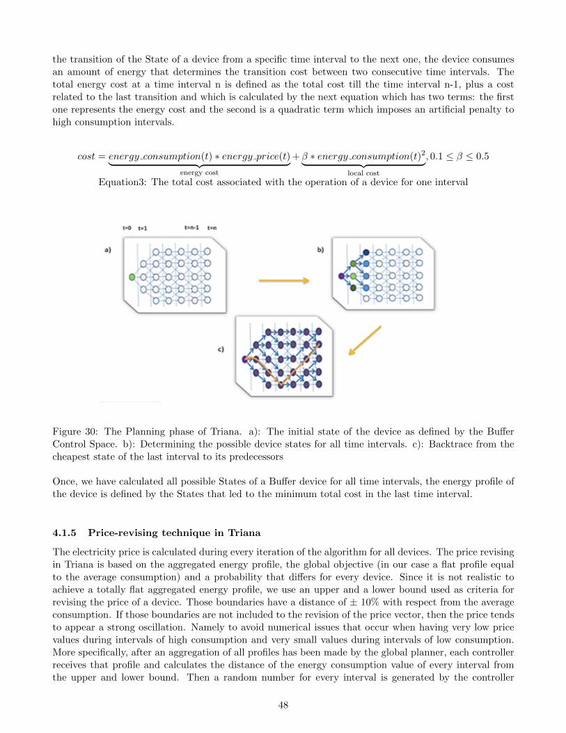
the transition of the State of a device from a specific time interval to the next one, the device consumesan amount of energy that determines the transition cost between two consecutive time intervals. Thetotal energy cost at a time interval n is defined as the total cost till the time interval n-1, plus a costrelated to the last transition and which is calculated by the next equation which has two terms: the firstone represents the energy cost and the second is a quadratic term which imposes an artificial penalty tohigh consumption intervals.

cost = energy consumption(t) ∗ energy price(t)︸ ︷︷ ︸energy cost

+β ∗ energy consumption(t)2︸ ︷︷ ︸local cost

, 0.1 ≤ β ≤ 0.5

Equation3: The total cost associated with the operation of a device for one interval

Figure 30: The Planning phase of Triana. a): The initial state of the device as defined by the BufferControl Space. b): Determining the possible device states for all time intervals. c): Backtrace from thecheapest state of the last interval to its predecessors

Once, we have calculated all possible States of a Buffer device for all time intervals, the energy profile ofthe device is defined by the States that led to the minimum total cost in the last time interval.

4.1.5 Price-revising technique in Triana

The electricity price is calculated during every iteration of the algorithm for all devices. The price revisingin Triana is based on the aggregated energy profile, the global objective (in our case a flat profile equalto the average consumption) and a probability that differs for every device. Since it is not realistic toachieve a totally flat aggregated energy profile, we use an upper and a lower bound used as criteria forrevising the price of a device. Those boundaries have a distance of ± 10% with respect from the averageconsumption. If those boundaries are not included to the revision of the price vector, then the price tendsto appear a strong oscillation. Namely to avoid numerical issues that occur when having very low pricevalues during intervals of high consumption and very small values during intervals of low consumption.More specifically, after an aggregation of all profiles has been made by the global planner, each controllerreceives that profile and calculates the distance of the energy consumption value of every interval fromthe upper and lower bound. Then a random number for every interval is generated by the controller

48

and if the distance mentioned is larger than the probability, then the price changes according to a pricedifference defined in the controller. The price difference is positive if the distance from the upper boundis positive or negative if the distance from the lower bound is negative. That procedure is followed forevery time interval.

4.1.6 Local planning: a pseudocode representation

The next pseudocode snippet presents how Dynamic Programming is applied in the current implemen-tation. This code presents the main task of a local Triana Controller bound to a Buffer device i.e. todetermine the energy consumption of a device based on the global objective and the total energy costduring the operation of a device. The outcome of the process presented is an energy profile which containsthe energy consumed during every interval. The first state of the Buffer device is explicitly defined bythe Buffer Control Space that is provided by the RAI. Based on that Control Space the states of the nextintervals are calculated. A different state is determined for every charge speed and it is considered validonly if the SoC is between 0 and 1. When the states of every time interval are calculated, we determinethe state of the last interval that resulted in the minimum total cost. The final step includes a backtraceto the previous intervals to find all predecessor states that led to the state with the minimum total cost.The returned energy profile contains a value that shows the energy consumption during every interval.Note that this information is stored in the states.

Algorithm: Dynamic Programming in local Triana PlanningInput: Heat Demand, Buffer Control Space (BCS), number of time intervals NObjective: Find and return the energy profile that leads to minimum energy cost

Local Planningcreate energyProfile, Time Interval array //length N=number of time intervals

for i=0 to N-1 do

if i=0

first State = initialState(BCS)

interval[i] ← first State

else

for State in interval[i].States

State.nextStates //every State of an interval creates a number of successor States

for all successors

if successors is valid

interval[i].addState

end if

end for

end for

end if

end for

find endState //the State with the minimum total cost in the last interval

energyProfile←backTrace(endState)//find the end States predecessors and determine the energyProfile

return energyProfile //the energyProfile that leads to minimum total cost

end Local Planning

49

4.1.7 Time Shifters

The algorithm developed for planning the operation of Time Shifter devices differs in some points to thealgorithm developed for the Buffers as the Control Space of these types differs. These differences areexplained in this subsection.

As described in the previous chapter, the Time Shifter Control Space is determined by the attributesstartAfter, startBefore and energyProfile. The first two variables are objects of the Java class Date whichshows how many milliseconds have elapsed from the 1st January 1970 and define an exact date and time.The energyProfile consists of pairs of values one of them showing an amount of energy consumption andthe other showing the duration in which that amount of energy gets consumed.

Therefore, those attributes have to be translated in variables that fit to the algorithm of Triana whichuses the time interval notion to specify a timestamp during the planning horizon. Java provides a methodthat calculates the number of seconds (or hours or minutes) of a Date object that passed from the begin-ning of the current day. By dividing that number with the length of a time interval in seconds and byrounding that number, we can define how many intervals have passed from the beginning of the planninghorizon. By doing that for the variables startAfter and startBefore, we define them as integer numbersthat correspond to the number of the time interval they belong during the planning horizon.

Additionally, the energy profile as defined in RAI had to be translated in an energy profile which has anenergy value for every interval. RAI contains a method that can split an energy profile to subprofiles.Each of them, is defined by an offset time (or the starting time of the sub profile) and the duration of thesub profile. In our case the duration is equal to a time interval. The offset is an integer multiple of theinterval length. Another method of RAI is able to calculate the energy consumed during the sub profile,which is now the energy value of the interval.

In figure 31 we can see the form of a Time Shifter energy profile as defined in RAI and how it is split in subprofiles each one having a duration equal to the time interval. RAI defines a continuous (length-encoded)energy profile. This profile is defined by pairs of energy consumption and the duration in which thisenergy was consumed. For example during the minutes 4-38 (duration of 35 minutes) the Time Shifterconsumed 0.7 kWh and this is defined by the command:

EnergyProfile.create().add(Measure.valueOf (35,NonSI.MINUTE),Measure.valueOf (0.7,NonSI.KWH))

During this conversion of a RAI -type energy profile to a Triana-type energy profile, a control is madethat ensures that the operation of a Time Shifter does not end after the end of the planning horizon.That control is done using a variable representing the time interval that corresponds to the starting timeof the operation. If the operation time (also calculated in intervals) added to the starting time intervalexceeds the planning horizon, then a Triana energy profile cannot be determined.

50

Figure 31: The energy profile of a time shifter as defined by RAI (above) and the energy profile split indiscrete subprofiles with a duration equal to the time interval (15 min)

During Planning, for a given price profile and a time shifter profile we calculate where the energy profileshould be placed during the planning horizon in order to get the minimum cost. In other words, given aprice profile for the planning horizon we define the energy cost for all possible starting times. The startingtime that reslts in the minimum cost determines when the Timeshifter will begin to operate.

In the figure 32, three possible positions of a Time Shifter profile (in our case it was a hypothetical profileof a washing machine) are shown. The profile has a duration of 90 minutes that corresponds to 6 intervals.Only case 2) shows an acceptable position. Case 1) has a starting time before startAfter. Cases 3) endingtime slightly exceeds the planning horizon (begins at time interval 92). Case 2) represents a feasiblestarting time and also represents the optimum solution regarding the energy cost as the price vector hasthe minimum price over the operation intervals.

51

Figure 32: Placing an energy profile in the optimum position of the planning horizon

4.1.8 Uncontrolled devices

The implementation of Planning phase for Uncontrolled devices is simpler compared to Buffer and TimeShifter devices.

The energy profile that belongs to an uncontrolled device is filled with energy values that correspondto the production or consumption of such a device. No alterations can be done to the profile of an un-controlled device. Its planning process returns to the Global Planner the energy profile that is shapedas described. In simulations executed in this assignment, an installation of PVs is represented as anuncontrolled device. The production values during a winter day were used to define its profile.

Finally it should be mentioned that the price-revising scheme used for Time Shifters is the same as for theBuffer devices, whereas the price-revising is not applied for Uncontrolled devices as there is no optimumcost solution that can be found for them. However they influence indirectly the price for the other deviceswith their contribution to the aggregated profile.

4.2 Incompatibilities between Triana and FPAI

To implement Triana using the FPAI there are several incompatibilities that have to be overcome.

Firstly we need to explain why Triana cannot directly be run on top of FPAI a fact that makes thebridging between Triana and FPAI more complex. Trianas planning phase uses parameters that are cal-culated during the first step of forecasting. FPAI does not yet contain a forecasting step that can providesuch functions and thus certain data were passed to Triana by using data files for e.g. the heat demand,necessary to implement the planning step for the buffer devices. Another example is the startAfter andstartBefore notions that were described in the previous section that were also passed manually and cor-respond to the information that would be given by the Resource Manager to a local Triana Controller.

Another incompatibility is the form the Time Shifter Control Space has, as provided by FPAI. The TimeShifter Control Space sends an energy profile that is continuous in time. Triana needs to receive anenergy profile consisting of values that show the energy consumption of each interval. This problem wassolved using a method provided by FPAI which can split an energy profile to sub profiles as explainedin subsection 4.1.7.. Furthermore, FPAI does not take into account the end of the planning horizon andthus the operation of a device could take place outside the planning horizon which is unacceptable forTriana. The control explained in figure 32, was the solution to that problem.

52

One more difference is the form of an Allocation and the form of an energy profile that is provided by Tri-ana as input. The difference is that Triana uses discrete time intervals (of the same duration) for each ofthose intervals an energy value is defined that shows the energy consumed during the interval. In contrary,the Allocation contains an energyProfile, defined by a list of energy/duration tuples where the duration isnot equal for all elements of the list. Thus, in our case the Allocation consists of an array with size equalto the time intervals of the planning horizon and a value showing the energy consumption in every interval.

Additionally, an incompatibility between FPAI and Triana is that FPAI uses in its energy calculationsonly electricity properties. Thus all Triana attributes that expressed energy in the form of heat had to beconverted in electricity. For example although Triana uses the Coefficient of Performance (COP) of a heatpump to calculate the SoC of a heat buffer based on the heat stored in it and the heat demand, in thecurrent implementation the COP was not used and instead we took into account the COP to convert theheat demand of a house to electricity demand. Auxiliary heat devices were also not taken into account.Auxiliary devices are used in Triana to cover the heat demands in the extreme case where the heat storedin the buffer and the energy consumed by the heat pump are not enough to the heat demand during oneinterval. If auxiliary devices are used, an extra penalty is posed to the total energy cost.

Another incompatibility that should be taken into account when thinking for a full implementation ofTriana (all phases) on top of FPAI is when a new Planning process should take place. Currently Trianauses data from the Forecasting phase to conduct the Planning for the next 24 hours with a rolling horizonof six hours. Nevertheless, the input which is now the Control Space can be changed in an arbitrarymoment as a new Control Space is generated as soon as a new measurement is done regarding one of theparameters that determine the flexibility of a device, e.g. the state of charge of a heat buffer or when anew program for a Time Shifter is entered.

Finally it should be mentioned that Triana is written in the software language C++ using the Qt plat-form, whereas FPAI is written in Java programming language. Thus, any core code of Triana that hadto be used has to be rewritten in Java as well as all other code developed to added extra functionality tothe Triana code so that Triana can use as input data or methods provided by the FPAI.

4.3 Software tools provided by the FPAI

In this section some of the software tools that FPAI provides are described and their usage during theimplementation of Trianas Planning phase.

FPAI uses a tool that makes calculations that include measurable properties more convenient - Measur-able interface. With Measurable we can express any property in a SI or a non SI unit and using anymultiplication factor. For example, in order to define that the capacity of a heat buffer is 10 kWh we usethe command:

ConstraintList<Power> cl = ConstraintList.create(SI.WATT).addSingle(1000) .addRange(2000, 3000).build;

For specifying all possible charge speeds of a heat buffer a class ConstraintList has been developed. Itcan define a series of single values or a range between which a heat pump could operate. For examplethe following constraint list represents a device which can consume 1000 watts and any amount between2000 and 3000 watts.

ConstraintList<Power> cl = ConstraintList.create(SI.WATT).addSingle(1000) .addRange(2000, 3000).build;

53

The sub profiles of the Time Shifters use the method:

subprofile (Measurable<Duration> offset, Measurable<Duration> duration)

where offset is in our case an integer multiple of a time interval and duration has the value of the lengthof a time interval.

4.4 The Class diagram of the code developed

In the appendix A of this document the Class diagram of the code developed is given in the form of aUnified Model Language (UML) diagram. A few remarks are put in this section to justify this specificstructure of the Class diagram.

4.4.1 The Timeseries super class and its sub-classes

The Timeseries super class uses the planning horizon and the time interval length to calculate the numberof time intervals of the planning horizon. Then, an array with size equal to the number of intervals isdefined. The sub classes EnergyProfile, PriceProfile and HeatDemand, need such an array to store a valuefor each time interval. For example an EnergyProfile object stores a value in every element of the arrayand these values represent the consumption (or production) of a device. The aggregated energy profileis also an object of the same type holding in each array element the aggregated energy consumption ofan interval. Similarly a PriceProfile object needs such an array to store the energy price values of eachinterval and a HeatDemand object the heat demand during each interval. In the Timeseries class twomethods are written that are used to read from and write to CSV files in order to read necessary data forour algorithm (e.g. the heat demand profiles of the houses) or to extract data from the simulations run.

4.4.2 The State and TimeInterval classes

These two classes are only used in the planning implementation for Buffer devices. As mentioned inthe previous section a State object contains all information that specifies the characteristics of the heatbuffer (SoC, buffer capacity, charge speeds) but also methods and variables used to calculate the energyconsumption during a transition from a State to another and the corresponding cost of this transition.Each TimeInterval object is composed of a number of States. A method makes sure that when two Stateshave the same SoC, only the one with the minimum cost is stored. A TimeInterval is also responsible forfinding the State of a time interval with the minimum total cost. This is used during the planning to findthe cheapest State of the last time interval. That is the state we use, to find its predecessors that finallydetermine the optimal energy profile (this energy profile results in the minimum total cost). The usageof these two classes makes it easier to split different tasks, which are necessary to determine the desiredenergy profile, to more than one components-objects thus improving the structure and readability of thecode and making it also easier to add extensions to it.

4.4.3 The TrianaController Interface, its implementations and the GlobalPlanner

The TrianaController interface contains three methods. One of them is the execution of planning fora single device and all classes that implement the interface have a different version of this method asdescribed in the previous sections of this chapter. The two other methods are only implemented for theBuffer and the Time Shifter Controller. These two methods are responsible for creating an initial priceprofile and to updating the price profile for the next iteration.

54

The TrianaController implementations receive the Control Space of a device typically by the ResourceManager and execute the Triana algorithm using that information in order to return an Allocation theenergy profile of the device. The Resource Manager is the connecting link between the device and anenergy application. Similarly to the BufferTrianaController, in Powermatchers implementation a BufferAgent is responsible for exploiting the Control Space of a buffer device.

The GlobalPlanner has a list of TrianaControllers. The first action of the GlobalPlanner is to definewhat kind and how many devices it will have under control defining the same time the data that need tobe read by the local controllers. For example the Triana Controllers of Buffer devices need to read theheat demand data of a house. PV Triana Controllers need to read the data that give the PV productionduring the planning horizon. When the process of Planning for all devices begins, the Buffer and TimeShifter devices receive an initial price and then they execute their planning algorithms. Finally the GlobalPlanner calculates the total mismatch and gives a command to the Triana Controllers to update theirprice profiles given the aggregated energy profile.

Conclusions

During the implementation of Trianas Planning phase, a part of the core functionality of the current Trianaimplementation was re-implemented in a way that the communication with FPAI could be made possible.Furthermore, several changes and additions were also necessary especially for the implementation of thePlanning phase of Triana regarding the Time Shifter devices (section 4.1.5). Other incompatibilities alsoincluded the data type that normally Triana uses and the data type as provided by FPAI. The flexibility ofa device is now revealed by its Control Space instead of the energy parameters that are normally providedby the Forecasting step of Triana. Triana is now able to handle a Control Space and execute the Planningphase for a fleet of devices.

The simulations of the next chapter prove that the implementation developed, produces the results thatare normally expected when the Planning of Triana is executed.

55

5 Simulations Results

In subsections 2.1.4 a series of simulations conducted within [4] were presented. Those simulations give anidea of what could be achieved through the control of a fleet of devices using Triana. A typical goal thatis set when using Triana to control a number of devices is to achieve an aggregated energy consumptionprofile that is flatter compared to the case when no control is used. In this chapter we present a seriesof simulation that were executed to test the software developed within this thesis which implements thePlanning phase of Triana using the FPAI.

5.1 General information about the simulations

The target during the simulations conducted in this thesis was to reach a flat profile regarding the energyconsumption of the devices controlled over a planning horizon. The flat profile means that aggregatedenergy consumption of all devices is steady over the planning horizon and has a value of Eav, where Eavis the average energy consumption of all devices.

As we normally will not be able to reach this profile, we aim at minimizing the mismatch from this profile.The mismatch can be calculated using the next equation of squared mismatch that measures how muchthe actual profile deviates from the average consumption.

SquaredMismatch =∑N

i=1(E(i)− Eav)

where

• N is the number of time intervals of the planning horizon,

• E(i) is the aggregated energy consumption of all devices at interval i,

• Eav is the average energy consumption of the aggregated profile (a targeted-flat profile)

An alternative measure for the mismatch could be the primary mismatch calculated by:

SquaredMismatch =∑N

i=1M(i), M(i) =

0.9Eav − E(i)ifE(i) < 0.9Eav

E(i)− 1.1EavifE(i) > 1.1Eav

0

In that case we calculate how much the actual profile deviates from and upper bound which is 1.1Eavanda lower bound which is 0.9Eav. In this assignment the mismatch was calculated using the formula of thesquared mismatch.

In figure 33 we show a real consumption profile (blue line) and the targeted profile which is the averageconsumption (red line). We also show the upper and lower boundaries which are the references for mea-suring the primary mismatch.

56

Figure 33: The real energy profile, the targeted-average consumption and the upper and lower bounds

In the following pages the graphs from a series of simulations are presented and explained. First wepresent simulations from the planning of a number of heat pumps accompanied by a heat buffer (Bufferdevices). Simulations are run for different buffer sizes and initial state of charge. Then, simulationsare done for houses that are equipped with heat pumps and a washing machine (Time Shifter devices).Finally we see the behavior of Triana when in the whole system we introduce the energy production fromPVs. All simulations included 30 iterations of the algorithm. The planning horizon is 24 hours and thetime interval length is 15 minutes, resulting in 96 intervals during the planning horizon.

5.2 Simulations

5.2.1 Planning for Buffer devices, Simulation 1

In this first simulation, we control the operation of twenty heat pumps using Triana. Each of the heatpumps is responsible for providing the energy required to cover the heat demand of one house. The heatpumps are connected to a heat buffer whose size is 10 kWh el (30 kWh th, COP=3). The heat pumpscan consume one to five kW with a step of one kW. The initial SoC of the buffers is zero.

Real data that represent the heat demand of a Dutch household for a winter day (collected in 2007) wereused. The heat demand of each house has a profile with high peaks at certain hours of the day and zero de-mand during other periods (figure 34). That would lead to a corresponding electricity profile if heat pumpsconsumed energy according to the heat demand. In figure 34 the heat demand of one house is shown.The abscissa of every point is the time interval and the ordinate the energy consumed during that interval.

57

Figure 34: The heat demand of a single house

Figure 35 shows the resulting energy consumption profile of the 20 heat pumps when the algorithmdeveloped is executed for two iterations. The energy profile presents very important oscillations regardingthe energy consumption through the planning horizon. The aggregated profile is improved after the5th algorithm iteration but the energy profile has still a wave shape with significant periods of peakconsumption (figure 36). The energy profile is much closer to the targeted profile after the 30th iterationas can be seen in figure 37. The red line in every graph represents the average consumption which is ourtarget profile.

Figure 35: Initial SoC=0, Buffer Size=10 kWh el, 2 iterations

58

Figure 36: Initial SoC=0, Buffer Size=10 kWh el, 5 iterations

Figure 37: Initial SoC=0, Buffer Size=10 kWh el, 30 iterations

The three profiles have a decreasing squared mismatch as the number of iterations increase; an expectedresult as it shows that the algorithm tries to achieve the global objective which is reaching an aggregatedenergy profile as close as possible to the average energy consumption. The graphs of the 2nd and 5thiteration have significantly higher peak consumption periods compared to the graph which shows theaggregated energy profile after the 30th iteration. The squared mismatch converges to a value close to 22already after the 10th iteration of the algorithm as can be seen from the next graph (figure 38).

59

Figure 38: Initial SoC=0, Buffer Size=10 kWh el, squared mismatch

Table 3 summarizes the results of the first simulation regarding the mismatch from the targeted profile.

Table 3: The squared mismatch in different iterations

The same conclusion can also be derived from the next graph which shows the aggregated energy profileafter 2, 5, 10, 20, 30 iterations. The high peaks after the 2nd (dark blue) and 5th (red) iteration areeliminated after the 10th iteration (figure 39).

60

Figure 39: Initial SoC=0, Buffer Size=10 kWh el, aggregated energy profiles

A common characteristic for all graphs is that the energy consumption has a steep reduction during thelast 5-10 time intervals (except for the case of the 2nd iteration when the algorithm has not influencedsignificantly the whole consumption). A simple explanation would be that the energy price signal is veryhigh during those intervals and that this cost increase reflects to the energy consumption. Neverthelessthat is not true. On the contrary, the energy cost during those intervals is respectively much lower com-pared to the energy price of the previous intervals. However the stored energy of the heat buffer is enoughto cover the heat demand and thus the heat pumps do not need to consume further energy for the lastintervals.

As an example the next graph (figure 40) shows the aggregated electricity consumption (primary axis)and the aggregated electricity price which is the sum of al price signals over all devices (secondary axis).The reduction in the price during the last intervals does not result to an increasing energy consumption(as would be expected) because the heat pumps are not turned on during these intervals as the heatdemand can be covered by the heat stored in the heat buffers. Thus in the last intervals the electricityprice and consumption appear a parallel reduction. Figure 41 shows the average price compared to theprice of one controller and the aggregated price of all controllers.

61

Figure 40: Aggregated energy consumption and the aggregated electricity price

Figure 41: Price of one controller and average price of all controllers

62

5.2.2 Planning for Buffer devices, Simulation 2: influence of the initial State of Charge

The input of simulation 1 was only changed in the initial state of charge of the buffers which was set to0.5. The influence of the initial state of charge of the buffers is examined regarding the average energyconsumption and the squared mismatch during the execution of the Planning phase of Triana applied to20 heat pumps.

Figure 42 and figure 43 show the aggregated energy profile after the 2nd and 30th iterations respectively.

Figure 42: Initial SoC=0.5, Buffer Size=10 kWh el, 2 iterations

Figure 43: Initial SoC=0.5, Buffer Size=10 kWh el, 30 iterations

Figure 44 shows the decrease of the squared mismatch as the number of algorithm iterations increases.

63

Figure 44: Squared mismatch, Initial SoC=0.5

Table 4 sums up the results from the two simulations performed. It can be concluded that when the initialSoC of the buffers was set to 0.5, the squared mismatch was reduced as a result of the larger flexibilityoffered by a buffer which has an initial SoC of 0.5 compared to a buffer with initial SoC of 0 which is forcedto consume energy in the initial time intervals as it holds the minimum SoC. Furthermore, the averageenergy consumption is smaller as a result of the stored energy in the buffer. The peak consumption is alsosignificantly reduced, probably because the high heat demand during certain intervals is partially coveredfrom the energy that is already stored from the beginning and thus less energy needs to be consumedduring that intervals.

Table 4: Comparison, Simulations 1 and 2 (Buffer size = 10 kWh el)

64

5.2.3 Planning for Buffer devices, Simulation 3: influence of the heat buffer size

The input was the same as simulation 2 except the capacity of the buffers which was changed to 5 kWh el(15 kWh th ,COP=3), which is half of the buffer size of simulation 2, allowing us to derive conclusionsregarding the influence of the buffer size to the aggregated energy profile.

Figure 45 shows the aggregated energy profile after 30 algorithm iterations and figure 46 the squaredmismatch over the planning horizon.

Figure 45: Initial SoC=0.5, Buffer Size=5 kWh el, 30 iterations

Figure 46: Squared mismatch: SoC=0.5, Buffer Size=5 kWh el

Table 5 compares the simulations 2 and 3. In these simulations the initial SoC was the same (0.5) but

65

the buffer size in simulation 3 was half of that of simulation 2.

Table 5: Comparison, Simulations 2 and 3 (initial SoC=0.5)

It can be derived that when the buffer size was reduced, the squared mismatch and the peak and averageconsumption increased. That is an expected result as the flexibility of a buffer increases with an increasingcapacity. The average consumption is also larger in the case of the smaller buffer as less energy is storedinitially.

5.2.4 Planning for Buffer and Uncontrolled devices, Simulation 4

In this simulation we added a PV system to the twenty houses equipped with heat pumps and buffers(buffer size = 10kWh el, initial SoC=0.5).

The data related to the PV production were received from a real system of 1.4 kWp during a winter day(of a house located in the Netherlands) and were multiplied by 50 and 100 to represent systems of 70kWp and 140 kWp respectively. We need to mention that because the data were received during a winterday, the PV system did not reach the maximum power it could produce during the measurements. Datafrom a winter day were chosen as the data for the heat demand were also collected during winter day.The PV production profile can be seen in figure 50 (yellow color).

The goal is again to reach a flat aggregated profile exploiting the same time the energy produced by thePV system. The next figures (figure 47 and figure 48) represent the aggregated profiles in the two casesof 70 and 140 kWp after 30 iterations.

66

Figure 47: PV capacity of 70 kWp

Figure 48: PV capacity of 140 kWp

The results regarding the squared mismatch and the peak and average consumption of the two cases aresummed up in table 6. The squared mismatch presents a very small difference between the two cases of70 and 140 KWp cases. The average consumption is smaller in the 140 kWp case as the energy offeredfrom the PV system to the buffer is larger. In both cases the average consumption is smaller comparedto the system where the PV system did not exist since the PVs cover part of the electricity demand. Thesquared mismatch is also decreased.

67

Table 6: Comparison: 0, 70, 140 kWp PV production)

5.2.5 Planning for Buffer, Uncontrolled and Time Shifter devices, Simulation 5

In this simulation we add twenty washing machines to the system of simulation four (one per house). Thesimulation also includes the PV production of 140kWp. The algorithm produces again satisfying resultsas the mismsatch converges again around the 10th iteration as can be seen in figure 50. Figure 49 showsthe aggregated energy profile after the 2nd and the 30th iteration.

Figure 49: The aggregated energy profile after the 2nd and 30th iteration

68

Figure 50: Squared mismatch, simulation 5

It would also be interesting to compare the energy consumed by the heat pumps and the washing ma-chines, with the energy produced by the PV system. In figure 51 the energy consumed by the heat pumpsis shown above the energy produced by the PV system. The peak consumption occurs to take advantageof the high PV production during the same period and by doing so the overall aggregated consumptiondoes not result in any peak consumption period during those intervals.

In figure 52 the energy consumed by the heat pumps and the washing machines is shown. The restrictionsposed by the permissible starting times, forces the washing machines to operate during a certain periodand that explains why all washing machines operate between the 48th and 82nd intervals. This fact canalso be seen in the aggregated consumption of the washing machines, shown in figure 53. By comparingthe graphs of the heat pump consumption and washing machine consumption we can see that in theperiods when the washing machines are turned on, the heat pumps have a very low overall consumptionto counterbalance the large energy consumption of the washing machines.

69

Figure 51: Aggregated heat pump consumption, PV production and total consumption

Figure 52: The aggregated energy consumed by the 20 heat pumps and the 20 washing machines

70

Figure 53: The energy consumed by the washing machines (stacked profiles)

5.3 Evaluation - Conclusions

The goal of the simulations executed and presented in this section, was to examine if the software de-veloped within this assignment, implements successfully the Planning phase of Triana. The objective inevery simulation was to control a number of devices, aiming at a flat aggregated consumption profile.

Simulations 1-3 included the control of Buffer devices. Simulations 2 and 3 examined the influence of theinitial state of charge and heat buffer size to the overall operation of the Buffer devices. In simulation4, the PV production added to the system of Buffer devices represented an Uncontrolled device. Finally,simulation 5 included twenty Time Shifter devices to the system of Buffer and Uncontrolled devices.

The results of all simulations showed that the execution of the algorithm developed produced the desiredresults; the mismatch between the actual and the goal profile, decreased with the number of running iter-ations. A convergence of the mismatch was also observed after a certain number of algorithm iterationsshowing that no further improvement can be achieved after this number of iterations.

71

6 Conclusions and future work

The goal of this thesis was to research whether it is possible to develop a software programme that im-plements the planning phase of Triana using the FPAI platform.

The first step to answer that question was a detailed study of Triana and FPAI. The study of Triana refersto both the theoretical background which includes the structure of Triana as well as the mathematicaltools that it is built on but also to the programming implementation of the planning phase. RegardingFPAI, FAN provides a series of documents that describe all platform specifications. Understanding theRAI software implementation of FPAI was also essential as every energy application that is built on FPAIneeds to understand the device flexibility as it is described by the Control Spaces but also because RAIprovides all the other tools given in Chapter 4.

The next step was the development of the software that would execute the planning phase of Trianausing the FPAI. Part of the software was developed during the internship conducted at TNO. During theimplementation a few incompatibilities were observed between Triana and FPAI as discussed in Chapter4. For the software development the core Triana functionality was used as a base. Nevertheless, newapproaches were used as to overcome certain problems like in the Time Shifter planning algorithm. Anumber of simulations were also executed to test if this specific implementation produced the expectedresults that the planning phase of Triana should result in.

This thesis showed that FPAI provides all necessary tools to expose the flexibility of devices in a mannerthat can be handled by Triana in order to execute its planning phase.

This thesis addressed the issue of implementing the planning phase of Triana only and not the imple-mentation of the other two phases of Triana, Forecasting and Real-time Control. FPAI does not includeyet a component that would be able to forecast the energy parameters (e.g. the heat demand for theplanning of Buffer devices or the permitted starting times for Time Shifter devices) that describe theenergy flexibility of the devices in the form that the existing Triana implementation needs to execute thenext phase, planning. To overcome this problem static heat demand profiles were used (Buffer devicecase) or the Control Space was used to provide essential information for the planning of other devices(e.g. the Time Shifter Control Space determines the permitted operation times). The execution of theForecasting and the Real-time Control phases of Triana could be subjects for future master theses as theresearchers working on the FPAI development have also considered the development of a platform that iscapable of producing forecasts related to the operation of the devices.

Another possibility for future work could be a comparison of Triana and Powermatcher implementationswhen executed using the FPAI platform. Such a comparison would expose the advantages/disadvantagesof each methodology over the other and would provide useful information for their improvement.

72

References

[1] Co2 in atmosphere per year. http://www.documentary-video.com/resources/documents/289.

jpg.

[2] ABB. Efficiency - along the whole value chain. Website. Available online at http://new.abb.com/smartgrids/why-smart-grids/efficiency, Accessed: June 2014.

[3] R.N. Anderson, A Boulanger, W.B. Powell, and W. Scott. Adaptive stochastic control for the smartgrid. Proceedings of the IEEE, 99(6):1098–1115, June 2011.

[4] Vincent Bakker. TRIANA : a control strategy for Smart Grids : forecasting, planning and real-timecontrol. PhD thesis, Enschede, the Netherlands, January 2012.

[5] S. Bertolini, M. Giacomini, S. Grillo, S. Massucco, and F. Silvestro. Coordinated micro-generationand load management for energy saving policies. In Innovative Smart Grid Technologies ConferenceEurope (ISGT Europe), 2010 IEEE PES, pages 1–7, Oct 2010.

[6] C. Block, D. Neumann, and C. Weinhardt. A market mechanism for energy allocation in micro-chpgrids. In Hawaii International Conference on System Sciences, Proceedings of the 41st Annual, pages172–172, Jan 2008.

[7] M. Bosman. Planning in Smart Grids. PhD thesis, University of Twente, 2012.

[8] BP. World energy consumption. Website. Available online at http://www.bp.com/en/global/

corporate/about-bp/energy-economics/statistical-review-of-world-energy.html, Ac-cessed: June, 2014.

[9] R. Caldon, AR. Patria, and R. Turri. Optimisation algorithm for a virtual power plant operation. InUniversities Power Engineering Conference, 2004. UPEC 2004. 39th International, volume 3, pages1058–1062 vol. 2, Sept 2004.

[10] M. Chertkov. Optimization and control theory for smart grids. Talk availble online at author’s site:http://cnls.lanl.gov/~chertkov/Talks/Grid/ColGrid.pdf. Accessed in: July 2014.

[11] L.M. Costa and G. Kariniotakis. A stochastic dynamic programming model for optimal use of localenergy resources in a market environment. In Power Tech, 2007 IEEE Lausanne, pages 449–454,July 2007.

[12] S. Dagioglou. A literature review on energy control methodologies. Capita Selecta Assignment forpartial fulifillment f the MSc of Sustainable Energy Technology, University of Twente, 2013.

[13] AL. Dimeas and N.D. Hatziargyriou. Agent based control of virtual power plants. In IntelligentSystems Applications to Power Systems, 2007. ISAP 2007. International Conference on, pages 1–6,Nov 2007.

[14] M. Erol-Kantarci and H. T. Mouftah. Wireless sensor networks in the smart power grid. Presentationin IEEE Ottawa Section Seminar, November 22 2010. Available online at: http://www.ieeeottawa.ca/comsoc/IEEESeminar-WirelessSensorNetworksWSNinPowerGrid-MErol-Kantarci.pdf.

[15] The Natural Resources Group. Average global temperature. http://www.thenrgroup.net/news/

images/Average-Global-Temperature.gif. Accessed: June 2014.

[16] D. J. Hammerstrom. Pacific northwest gridwisetm testbed demonstration projects. Prepared for U.S.Department of Energy by the Pacific Northwest National Laboratory, Richland, WA, 2007. Availableonline at http://gridwise.pnl.gov/docs/op_project_final_report_pnnl17167.pdf.

73

[17] M. P F Hommelberg, C.J. Warmer, I G. Kamphuis, J. K. Kok, and G.J. Schaeffer. Distributedcontrol concepts using multi-agent technology and automatic markets: An indispensable feature ofsmart power grids. In Power Engineering Society General Meeting, 2007. IEEE, pages 1–7, June2007.

[18] J. K. Kok, C. J. Warmer, and I. G. Kamphuis. Powermatcher: Multiagent control in the electricityinfrastructure. In Proceedings of the Fourth International Joint Conference on Autonomous Agentsand Multiagent Systems, AAMAS ’05, pages 75–82, New York, NY, USA, 2005. ACM.

[19] K. Kok. The Powermatcher: Smart Coordination for the Smart Electricity Grid. PhD thesis, VrijeUniversiteit, Amsterdam, 2013.

[20] A. Kooijman. Technology and sustainable development. Course lectures at SET progrmme, Univer-sity of Twente, 2014.

[21] Fan H. Lowe M. and Gereffi G. U.s. smart grid, finding new ways to cut carbon and create jobs.Center on Globalization, Governance & Competitiveness, Duke University, April 2011. Availableonlineat at http://gridwise.pnl.gov/docs/op_project_final_report_pnnl17167.pdf.

[22] Albert Molderink. On the three-step control methodology for Smart Grids. PhD thesis, Enschede,the Netherlands, May 2011.

[23] FlexiblePower Alliance Network. Flexiblepower application infrastructure developer tutorial, Novem-ber 2013. Available online at http://www.flexiblepower.org/downloads/.

[24] FlexiblePower Alliance Network. High level functional specification of the flexiblepower applicationinfrastructure, January 2013. Available online at http://www.flexiblepower.org/downloads/.

[25] Global Footprint Network. Footprint for nations. Website. Available online at: http://

www.footprintnetwork.org/en/index.php/GFN/page/footprint_for_nations/, Accessed: June2014.

[26] Global Footprint Network. Glossary. URL: http://www.footprintnetwork.org/en/index.php/GFN/page/glossary/. Accessed: June, 2014.

[27] Global Footprint Network. World footprint. Website. Available online at: http://www.

footprintnetwork.org/en/index.php/GFN/page/world_footprint/, Accessed: June 2014.

[28] Climate Action of European Commission. The 2020 climate and energy package. Website. Availableonline at http://ec.europa.eu/clima/policies/package/index_en.htm.

[29] United Nations World Population Prospects. World population. Available online at: http://esa.

un.org/wpp/unpp/panel_population.htm. Accessed: June, 2014.

[30] W. Saad, Zhu Han, H.V. Poor, and T. Basar. A noncooperative game for double auction-based energytrading between phevs and distribution grids. In Smart Grid Communications (SmartGridComm),2011 IEEE International Conference on, pages 267–272, Oct 2011.

[31] W. Saad, Zhu Han, H.V. Poor, and T. Basar. Game-theoretic methods for the smart grid: Anoverview of microgrid systems, demand-side management, and smart grid communications. SignalProcessing Magazine, IEEE, 29(5):86–105, Sept 2012.

[32] M.A Sofla and R. King. Control method for multi-microgrid systems in smart grid environment–stability, optimization and smart demand participation. In Innovative Smart Grid Technologies(ISGT), 2012 IEEE PES, pages 1–5, Jan 2012.

74

[33] V. Thompson. Using neural networks to create a new control methodology for smart grids. In Web-site of National Science Foundation, http://www.nsf.gov/discoveries/disc_summ.jsp?cntn_id=127605, April 2013. Accessed in: July 2014.

[34] Wikipedia. Electric energy consumption. Accessed: June, 2014.

[35] Wikipedia. Stochastic control. Accessed: 25-03-2013.

75

7Appendix−

Class

Diagra

m(U

ML)

76