an exact and grid-free numerical scheme ... - kaust...

An Exact and Grid-free Numerical Scheme for the

Hybrid Two Phase Traffic Flow Model Based on

the Lighthill-Whitham-Richards Model with

Bounded Acceleration

Thesis by

Shanwen Qiu

In Partial Fulfillment of the Requirements

For the Degree of

Masters of Science

King Abdullah University of Science and Technology, Thuwal,

Kingdom of Saudi Arabia

July, 2012

2

The thesis of Shanwen Qiu is approved by the examination committee

Committee Chairperson: Christian Claudel

Committee Member: Sigurdur Thoroddsen

Committee Member: Taous-Meriem Laleg

3

Copyright ©2012

Shanwen Qiu

All Rights Reserved

4

ABSTRACT

An Exact and Grid-free Numerical Scheme for the Hybrid

Two Phase Traffic Flow Model Based on the

Lighthill-Whitham-Richards Model with Bounded

Acceleration

Shanwen Qiu

In this article, we propose a new grid-free and exact solution method for com-

puting solutions associated with an hybrid traffic flow model based on the Lighthill-

Whitham-Richards (LWR) partial differential equation. In this hybrid flow model,

the vehicles satisfy the LWR equation whenever possible, and have a fixed acceler-

ation otherwise. We first present a grid-free solution method for the LWR equation

based on the minimization of component functions. We then show that this solution

method can be extended to compute the solutions to the hybrid model by proper

modification of the component functions, for any concave fundamental diagram. We

derive these functions analytically for the specific case of a triangular fundamental

diagram. We also show that the proposed computational method can handle fixed or

moving bottlenecks.

5

Acknowledgments

I would like to sincerely thank my supervisor Dr. Christian G. Claudel for his continu-

ous guidance and encouragement throughout the course of this work. His enthusiasm

and valuable feedback for research made my study very enjoyable and exciting and

ultimately fruitful with rich experience. I would also like to thank him for providing

me with an amazing research environment.

My great gratitude also goes to my friends and colleagues who have selfless and

generously helped me with my thesis.

I thank my parents for their continuous encouragement and my siblings for bearing

with me for my negligence towards them during this journey and their deep moral

support at all times.

Lastly, I would like to thank the people at KAUST, Thuwal, Makkah Province,

Saudi Arabia for providing support and resources for this research work.

6

TABLE OF CONTENTS

Examination Committee Approval 2

Copyright 3

Abstract 4

Acknowledgments 5

List of Figures 8

1 Introduction 9

1.1 Background . . . . . . . . . . . . . . . . . . . . . . . . . . . . . . . . 9

2 Modeling 12

2.1 The LWR PDE . . . . . . . . . . . . . . . . . . . . . . . . . . . . . . 12

2.2 The Moskowitz function . . . . . . . . . . . . . . . . . . . . . . . . . 13

2.3 Piecewise affine initial and boundary conditions . . . . . . . . . . . . 14

2.4 Affine internal boundary conditions . . . . . . . . . . . . . . . . . . . 15

3 Analytical Solutions to the Moskowitz HJ PDE and LWR PDE 16

3.1 Solutions to the Hamilton-Jacobi equation . . . . . . . . . . . . . . . 16

3.2 Solution components associated with affine conditions . . . . . . . . . 17

3.2.1 Initial conditions . . . . . . . . . . . . . . . . . . . . . . . . . 17

3.2.2 Upstream boundary conditions . . . . . . . . . . . . . . . . . 18

3.2.3 Downstream boundary conditions . . . . . . . . . . . . . . . . 18

3.2.4 Internal boundary conditions . . . . . . . . . . . . . . . . . . 19

3.3 Componentwise computation of the Moskowitz/LWR function . . . . 21

4 Analytical Derivation of Vehicle Trajectories 23

4.1 Initial conditions . . . . . . . . . . . . . . . . . . . . . . . . . . . . . 23

7

4.2 Upstream and downstream boundary conditions . . . . . . . . . . . . 24

4.3 Internal boundary conditions . . . . . . . . . . . . . . . . . . . . . . . 25

5 Definition of the Solution to the Two Phase LWR Flow Model with

Bounded Acceleration 27

5.1 The two phase bounded acceleration-LWR traffic flow model . . . . . 27

5.2 Properties of the solutions . . . . . . . . . . . . . . . . . . . . . . . . 29

5.2.1 Inf property . . . . . . . . . . . . . . . . . . . . . . . . . . . . 29

5.2.2 Structure of the resulting solutions . . . . . . . . . . . . . . . 30

5.2.3 Solution structure . . . . . . . . . . . . . . . . . . . . . . . . . 30

6 Analytical Derivation of the Modified Solution Components for the

Triangular Fundamental Diagram 32

6.1 Initial condition . . . . . . . . . . . . . . . . . . . . . . . . . . . . . . 33

6.1.1 Free-flow initial condition . . . . . . . . . . . . . . . . . . . . 33

6.1.2 Congested initial condition . . . . . . . . . . . . . . . . . . . . 34

6.2 Upstream boundary condition . . . . . . . . . . . . . . . . . . . . . . 35

6.3 Downstream boundary condition . . . . . . . . . . . . . . . . . . . . 37

6.4 Internal boundary condition . . . . . . . . . . . . . . . . . . . . . . . 38

7 Implementation 44

7.1 Algorithm structure . . . . . . . . . . . . . . . . . . . . . . . . . . . . 44

7.2 Numerical examples . . . . . . . . . . . . . . . . . . . . . . . . . . . . 46

7.3 Benefits of a grid-free and exact method . . . . . . . . . . . . . . . . 49

8 Conclusion 50

References 51

Appendices 55

8

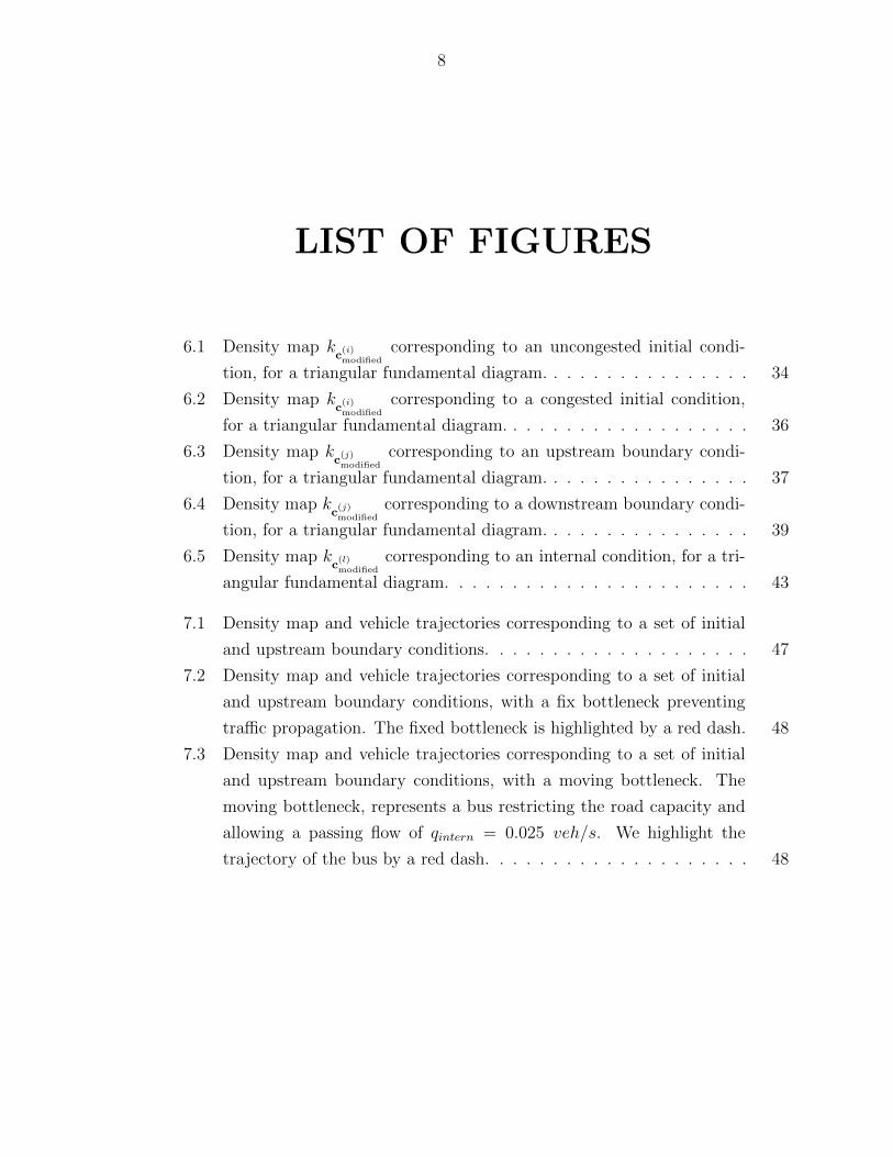
LIST OF FIGURES

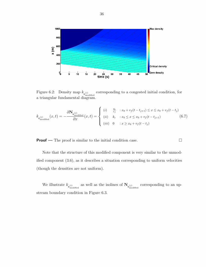
6.1 Density map kc

(i)modified

corresponding to an uncongested initial condi-

tion, for a triangular fundamental diagram. . . . . . . . . . . . . . . . 34

6.2 Density map kc

(i)modified

corresponding to a congested initial condition,

for a triangular fundamental diagram. . . . . . . . . . . . . . . . . . . 36

6.3 Density map kc

(j)modified

corresponding to an upstream boundary condi-


6.4 Density map kc

(j)modified

corresponding to a downstream boundary condi-


6.5 Density map kc

(l)modified

corresponding to an internal condition, for a tri-

angular fundamental diagram. . . . . . . . . . . . . . . . . . . . . . . 43

7.1 Density map and vehicle trajectories corresponding to a set of initial

and upstream boundary conditions. . . . . . . . . . . . . . . . . . . . 47


and upstream boundary conditions, with a fix bottleneck preventing

traffic propagation. The fixed bottleneck is highlighted by a red dash. 48


and upstream boundary conditions, with a moving bottleneck. The

moving bottleneck, represents a bus restricting the road capacity and

allowing a passing flow of qintern = 0.025 veh/s. We highlight the

trajectory of the bus by a red dash. . . . . . . . . . . . . . . . . . . . 48

9

Chapter 1

Introduction

1.1 Background

One of seminal traffic flow models for highways is presented in [1] and [2], and results

in the so called Lighthill-Whitham-Richards (LWR) model or kinematic wave theory.

Although more sophisticated models of traffic flow are available, the LWR model is

widely used to model highway traffic [3] and more recently for urban traffic [4]. The

LWR partial differential equation (PDE) is a first order scalar hyperbolic conservation

law that computes the evolution of a density function (the density of vehicles on a

road section). This PDE has multiple solutions in general, among which the entropy

solution [5] is recognized to be the physically meaningful solution.

While the LWR model is very robust, it fails to capture some observed features

of traffic such as traffic instabilities or kinematic constraints of real vehicles. In par-

ticular, the viscosity solutions [6] to the LWR model do not model the dynamics of

the vehicles [7] accurately, as the vehicle trajectories solutions to the LWR model

can exhibit unrealistically large accelerations or decelerations. These modeling errors

can have significant effects, for instance when computing the discharge rate of bot-

tlenecks [8, 9, 10], or when coupling [7, 11] vehicle models (fuel consumption, noise)

10

with traffic flow models.

These shortcomings led to a quantity of work in the field of higher order models,

such as the second order models [12, 13].the two phase flow model was introduced

in [9, 14], and was further developed in [7] for the case of fixed and moving bottlenecks,

where it was introduced as the field bounded acceleration model. In the two phase

flow model, the vehicles follow the LWR model in some areas of the computational

domain, while satisfying kinematic constraints (bounded acceleration) otherwise. The

formal definition (in terms of PDE) for such a model is particularly difficult: unlike

the case of ordinary differential equations, there is no general framework for solving

and even mathematically defining hybrid PDEs. As part of this article, we propose

a formal mathematical definition of the solution to the two phase flow model (or

equivalently field bounded acceleration model).

The LWR PDE itself can be numerically solved using a variety of computational

methods, such as first order numerical schemes, for instance in [15, 16, 17]. Classical

numerical methods often require a computational grid, and yield an approximate so-

lution of the PDE. Some exceptions exist however, such as the wave tracking methods,

see for instance [18], or semi-analytic algorithms [19, 20, 21]. In the present article,

we propose an modification of the semi-analytical algorithm introduced in [21] for

computing solutions to the hybrid two phase LWR model [9, 7]. This modification

preserves the fundamental advantages of the semi-analytical algorithm: exactness and

fast computational time.

The rest of this article is organized as follows. Section 2 defines the LWR and

HJ PDEs investigated in this article. Section ?? introduces the concept of partial

solutions to the HJ PDE. We show that these partial solutions can cause the accel-

eration (or deceleration) to become very large or unbounded. These partial solutions

are further modified to serve as the building blocks of the solution to the two phase

flow model, which is defined semi-analytically in Section 5. We further derive the ex-

11

pression of the partial solutions for the triangular fundamental diagram in Section 6,

and present a pseud-code implementation of the resulting numerical scheme. Finally,

we illustrate the performance of the algorithm on simulated traffic flow scenarios

including moving and fixed bottlenecks in Section 7.

12

Chapter 2

Modeling

2.1 The LWR PDE

We consider a one-dimensional, homogeneous section of highway, limited by x0 up-

stream and xn downstream. For a given time t ∈ [0, tm] and position x ∈ [x0, xn],

we define the local traffic density k(x, t) in vehicles per unit length, and the instan-

taneous flow q(x, t) in vehicles per unit time. The conservation of vehicles on the

highway is written as follows [1, 2, 22]:

∀x, t ∈ [x0, xn]× [0, tm],∂k(x, t)

∂t+∂q(x, t)

∂x= 0 (2.1)

For first order traffic flow models, flow and density are related by the fundamen-

tal diagram Q : (x, t, k(x, t)) 7→ q(x, t), which is an empirically measured law [23].

Through this article, we consider the homogeneous problem [24] in which the funda-

mental diagram is a function of density k only, i.e. q(x, t, k(x, t)) = Q(k(x, t)).

The fundamental diagram is a positive function defined on [0, κ], where κ is the

maximal density (jam density). It ranges in [0, qmax] where qmax is the maximum

flow (capacity). It is assumed to be differentiable at 0 and κ, with Q′(0) = vf > 0

the free flow speed, and Q′(κ) = w < 0 the congested wave speed [1]. We assume

13

that the fundamental diagram is concave and continuous. The introduction of the

fundamental diagram yields the Lighthill-Whitham-Richards (LWR) PDE :

∀x, t ∈ [x0, xn]× [0, tm],∂k(x, t)

∂t+∂Q(k(x, t))

∂x= 0 (2.2)

2.2 The Moskowitz function

The cumulated vehicle count N(x, t), also called Moskowitz function [25], represents

the continuous vehicle count at location x and time t. It has been developed for

instance in [3, 26, 24] in the context of transportation engineering, and goes back to

[27, 25].

In the Moskowitz framework, one assumes that all vehicles are labeled by increas-

ing integers as they pass the entry point x0 of a highway section, and that they cannot

pass each other. If the latest car that passed an observer standing at location x and

time t is labeled n, then bN(x, t)c = n. The Moskowitz function contains all traffic

information that one can infer from experimental traffic measurements as long as ve-

hicles do not pass each other. In this specific case, the isolines of N(x, t) correspond

to vehicle trajectories.

Moreover, local density k(x, t) and flow q(x, t) can be inferred from vehicle counts

using the formulas

k(x, t) = −∂N(x, t)

∂x(2.3)

q(x, t) =∂N(x, t)

∂t(2.4)

Introducing the Moskowitz function in (2.2) yields the Hamilton-Jacobi PDE [3,

26, 24, 19, 20, 21] in which the fundamental diagram Q plays the role of Hamilto-

nian [28]:

∂N(x, t)

∂t−Q

(−∂N(x, t)

∂x

)= 0 (2.5)

14

2.3 Piecewise affine initial and boundary condi-

tions

For the rest of the article, we use piecewise constant initial and boundary conditions

on density and flow, which translate to piecewise-affine conditions on the Moskowitz

function. Piecewise constant conditions on density and flow are a natural way to

encode discrete measurements in the model, and are used for instance in the Cell

Transmission Model (CTM) [16] and the associated Godunov scheme [15].

Let m and n ≥ 1 be integers, x0 < x1 < · · · < xn and t0 < t1 < · · · < tm the space-

time discretization for initial and boundary conditions where t0 = 0. We assume that

the initial densities (k(i)ini)0≤i≤n−1 ∈ Rn

+, the upstream flows (q(j)up )0≤j≤m−1 ∈ Rm

+ and

the downstream flows (q(j)down)0≤j≤m−1 ∈ Rm

+ are given. The initial densities are thus

decomposed as piecewise constant in their respective measurement intervals:

∀x ∈ [xi, xi+1], k(x, 0) = k(i)ini (2.6)

and let the upstream and downstream flows also be prescribed as piecewise constant:

∀t ∈ [tj, tj+1[, q(x0, t) = q(j)up (2.7)

q(xn, t) = q(j)down (2.8)

Note that no assumption is made regarding the uniformity of the grid: the spacings

xi − xi−1 and ti − ti−1 are not necessarily uniform over i.

The initial condition of the Moskowitz PDE is obtained by integrating the initial

condition of the LWR PDE assuming that Nini(x0) = 0 and :

∀x ∈ [xi, xi+1],Nini(x) = −∫ x

x0

k(χ, 0)dχ = −i−1∑m=0

(xm+1−xm)k(m)ini −(x−xi)k(i)

ini (2.9)

15

Similarly, the upstream and downstream boundary conditions of the Moskowitz

PDE, assuming that Nup(0) = 0 and Nini(xn) = Ndown(0) are given by:

∀t ∈ [tj, tj+1],Nup(t) =

∫ t

0

qup(τ)dτ =

j−1∑m=0

(tm+1 − tm)q(m)up + (t− tj)q(j)

up (2.10)

∀t ∈ [tj, tj+1],Ndown(t) = Nini(xn)+

∫ t

0

qdown(τ)dτ = Nini(xn)+

j−1∑m=0

(tm+1−tm)q(m)down+(t−tj)q(j)

down

(2.11)

2.4 Affine internal boundary conditions

Similarly to the algorithm described in [21], our proposed algorithm can also integrate

any number of internal boundary conditions, which can be used to model fixed or

moving bottlenecks [29].

An affine internal boundary condition of the Moskowitz function is mathematically

defined as :

c(l)intern(x, t) = M (l) + q

(l)intern(t− t(l)min) : t

(l)min ≤ t ≤ t

(l)max and x = x(l) + V

(l)intern(t− t(l)min)

(2.12)

In the above formula, the internal boundary condition imposes an average maximal

passing rate of q(l)intern on the domain defined by t

(l)min ≤ t ≤ t

(l)max and x = x

(l)min +

V(l)

intern(t− t(l)min). It can represent in practice a fixed (V(l)

intern = 0) or a moving (V(l)

intern >

0) bottleneck, restricting the relative capacity of the road to q(l)intern on its path.

16

Chapter 3

Analytical Solutions to the

Moskowitz HJ PDE and LWR

PDE

3.1 Solutions to the Hamilton-Jacobi equation

In order to compute the analytical solution of equation (2.5) with conditions of the

type (2.9), (2.10), (2.11), and (2.12), we define (based on [24, 30]) the following convex

transform associated with the fundamental diagram:

∀u ∈ [w, vf ], R(u) = supk∈[0,κ]

(Q(k)− u · k) (3.1)

The function −R is the Legendre-Fenchel transform of the function Q (fundamen-

tal diagram).

17

3.2 Solution components associated with affine con-

ditions

In this section, we use the notation Q′ for the derivative of the fundamental diagram

(which only depends on one argument). Note that we have assumed earlier that Q

has a right derivative vf in 0 and a left derivative w in κ.

Following [21], we define below the partial components of the solutions for the

four types of value conditions.

3.2.1 Initial conditions

We want to compute the solution component induced by an affine, locally defined

initial condition indexed by i:

∀x ∈ [xi, xi+1], c(i)ini(x) = −kix+ bi (3.2)

with bi = kixi −∑i−1

l=0(xl+1 − xl)k(l)ini allowing for the continuity of the initial

conditions in (0, xi). Using the results of [20], the analytical solution to the problem

associated with this sole initial condition can be written as

Nc

(i)ini

(x, t) =

tQ(ki)− kix+ bi : xi + tQ′(ki) ≤ x ≤ xi+1 + tQ′(ki)

tR(x−xit

)− kixi + bi : xi + tw ≤ x ≤ xi + tQ′(ki)

tR(x−xi+1

t)− kixi+1 + bi : xi+1 + tQ′(ki) ≤ x ≤ xi+1 + tvf

(3.3)

kc

(i)ini

(x, t) = −∂N

c(i)ini

∂x(x, t) =

ki : xi + tQ′(ki) ≤ x ≤ xi+1 + tQ′(ki)

−R′(x−xit

) : xi + tw ≤ x ≤ xi + tQ′(ki)

−R′(x−xi+1

t) : xi+1 + tQ′(ki) ≤ x ≤ xi+1 + tvf

(3.4)

18

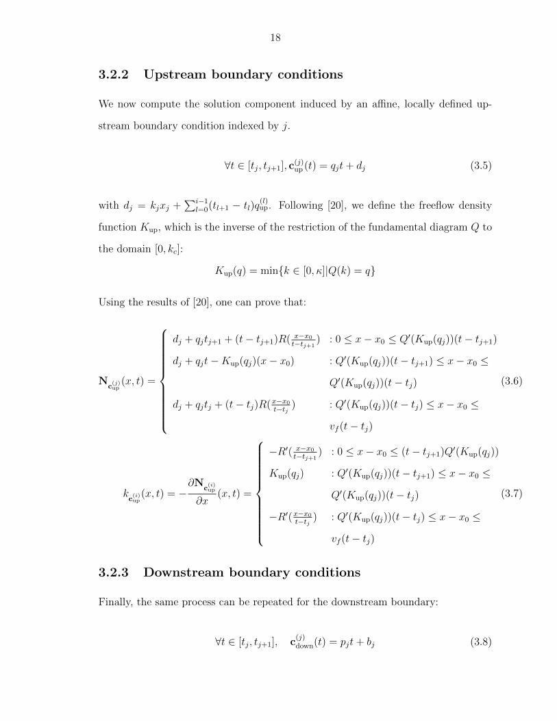
3.2.2 Upstream boundary conditions

We now compute the solution component induced by an affine, locally defined up-

stream boundary condition indexed by j.

∀t ∈ [tj, tj+1], c(j)up (t) = qjt+ dj (3.5)

with dj = kjxj +∑i−1

l=0(tl+1 − tl)q(l)up. Following [20], we define the freeflow density

function Kup, which is the inverse of the restriction of the fundamental diagram Q to

the domain [0, kc]:

Kup(q) = min{k ∈ [0, κ]|Q(k) = q}

Using the results of [20], one can prove that:

Nc

(j)up

(x, t) =

dj + qjtj+1 + (t− tj+1)R( x−x0

t−tj+1) : 0 ≤ x− x0 ≤ Q′(Kup(qj))(t− tj+1)

dj + qjt−Kup(qj)(x− x0) : Q′(Kup(qj))(t− tj+1) ≤ x− x0 ≤

Q′(Kup(qj))(t− tj)

dj + qjtj + (t− tj)R(x−x0

t−tj ) : Q′(Kup(qj))(t− tj) ≤ x− x0 ≤

vf (t− tj)

(3.6)

kc

(i)up

(x, t) = −∂N

c(i)up

∂x(x, t) =

−R′( x−x0

t−tj+1) : 0 ≤ x− x0 ≤ (t− tj+1)Q′(Kup(qj))

Kup(qj) : Q′(Kup(qj))(t− tj+1) ≤ x− x0 ≤

Q′(Kup(qj))(t− tj)

−R′(x−x0

t−tj ) : Q′(Kup(qj))(t− tj) ≤ x− x0 ≤

vf (t− tj)

(3.7)

3.2.3 Downstream boundary conditions

Finally, the same process can be repeated for the downstream boundary:

∀t ∈ [tj, tj+1], c(j)down(t) = pjt+ bj (3.8)

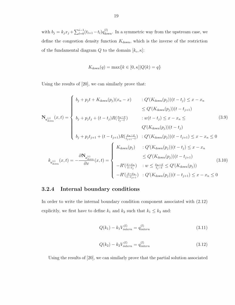
19

with bj = kjxj +∑i−1

l=0(tl+1− tl)q(l)down. In a symmetric way from the upstream case, we

define the congestion density function Kdown, which is the inverse of the restriction

of the fundamental diagram Q to the domain [kc, κ]:

Kdown(q) = max{k ∈ [0, κ]|Q(k) = q}

Using the results of [20], we can similarly prove that:

Nc

(j)down

(x, t) =

bj + pjt+Kdown(pj)(xn − x) : Q′(Kdown(pj))(t− tj) ≤ x− xn

≤ Q′(Kdown(pj))(t− tj+1)

bj + pjtj + (t− tj)R(xn−xtj−t ) : w(t− tj) ≤ x− xn ≤

Q′(Kdown(pj))(t− tj)

bj + pjtj+1 + (t− tj+1)R( xn−xtj+1−t) : Q′(Kdown(pj))(t− tj+1) ≤ x− xn ≤ 0

(3.9)

kc

(i)down

(x, t) = −∂N

c(i)down

∂x(x, t) =

Kdown(pj) : Q′(Kdown(pj))(t− tj) ≤ x− xn

≤ Q′(Kdown(pj))(t− tj+1)

−R′(x−xnt−tj ) : w ≤ xn−x

tj−t ≤ Q′(Kdown(pj))

−R′( x−xnt−tj+1

) : Q′(Kdown(pj))(t− tj+1) ≤ x− xn ≤ 0

(3.10)

3.2.4 Internal boundary conditions

In order to write the internal boundary condition component associated with (2.12)

explicitly, we first have to define k1 and k2 such that k1 ≤ k2 and:

Q(k1)− k1V(l)intern = q

(l)intern (3.11)

Q(k2)− k2V(l)intern = q

(l)intern (3.12)

Using the results of [20], we can similarly prove that the partial solution associated

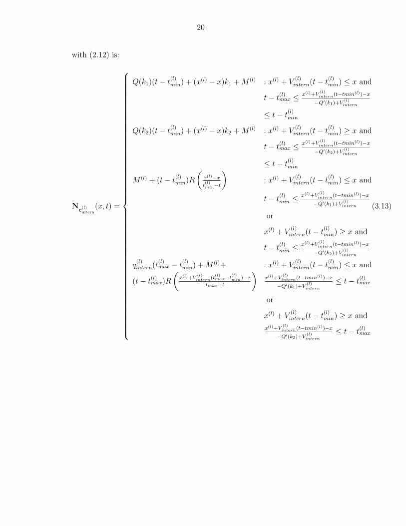
20

with (2.12) is:

Nc

(l)intern

(x, t) =

Q(k1)(t− t(l)min) + (x(l) − x)k1 +M (l) : x(l) + V(l)intern(t− t(l)min) ≤ x and

t− t(l)max ≤ x(l)+V(l)intern(t−tmin(l))−x−Q′(k1)+V

(l)intern

≤ t− t(l)min

Q(k2)(t− t(l)min) + (x(l) − x)k2 +M (l) : x(l) + V(l)intern(t− t(l)min) ≥ x and


(l)intern

≤ t− t(l)min

M (l) + (t− t(l)min)R

(x(l)−xt(l)min−t

): x(l) + V

(l)intern(t− t(l)min) ≤ x and

t− t(l)min ≤x(l)+V

(l)intern(t−tmin(l))−x−Q′(k1)+V

(l)intern

or

x(l) + V(l)intern(t− t(l)min) ≥ x and

t− t(l)min ≤x(l)+V


(l)intern

q(l)intern(t

(l)max − t(l)min) +M (l)+ : x(l) + V

(l)intern(t− t(l)min) ≤ x and

(t− t(l)max)R(x(l)+V

(l)intern(t

(l)max−t

(l)min)−x

tmax−t

)x(l)+V


(l)intern

≤ t− t(l)max

or

x(l) + V(l)intern(t− t(l)min) ≥ x and

x(l)+V(l)intern(t−tmin(l))−x−Q′(k2)+V

(l)intern

≤ t− t(l)max

(3.13)

21

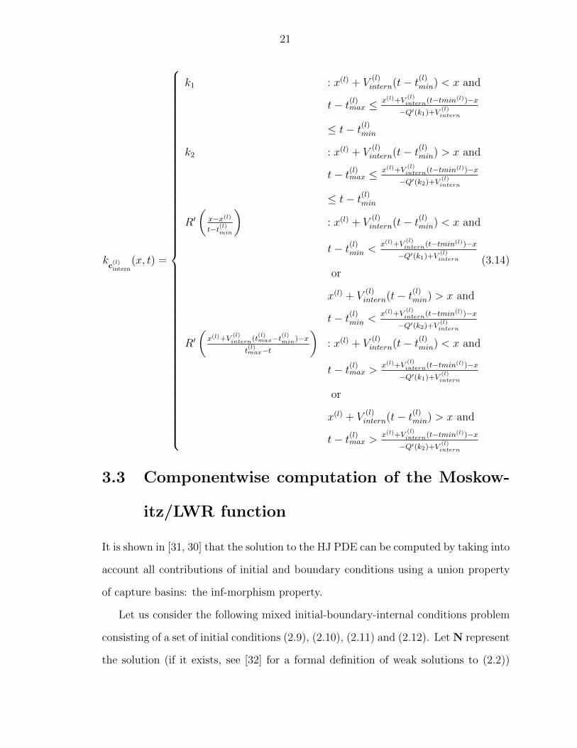
kc

(l)intern

(x, t) =

k1 : x(l) + V(l)intern(t− t(l)min) < x and


(l)intern

≤ t− t(l)min

k2 : x(l) + V(l)intern(t− t(l)min) > x and


(l)intern

≤ t− t(l)min

R′(

x−x(l)

t−t(l)min

): x(l) + V

(l)intern(t− t(l)min) < x and

t− t(l)min <x(l)+V


(l)intern

or

x(l) + V(l)intern(t− t(l)min) > x and

t− t(l)min <x(l)+V


(l)intern

R′(x(l)+V

(l)intern(t

(l)max−t

(l)min)−x

t(l)max−t

): x(l) + V

(l)intern(t− t(l)min) < x and

t− t(l)max > x(l)+V(l)intern(t−tmin(l))−x−Q′(k1)+V

(l)intern

or

x(l) + V(l)intern(t− t(l)min) > x and

t− t(l)max > x(l)+V(l)intern(t−tmin(l))−x−Q′(k2)+V

(l)intern

(3.14)

3.3 Componentwise computation of the Moskow-

itz/LWR function

It is shown in [31, 30] that the solution to the HJ PDE can be computed by taking into

account all contributions of initial and boundary conditions using a union property

of capture basins: the inf-morphism property.

Let us consider the following mixed initial-boundary-internal conditions problem

consisting of a set of initial conditions (2.9), (2.10), (2.11) and (2.12). Let N represent

the solution (if it exists, see [32] for a formal definition of weak solutions to (2.2))

22

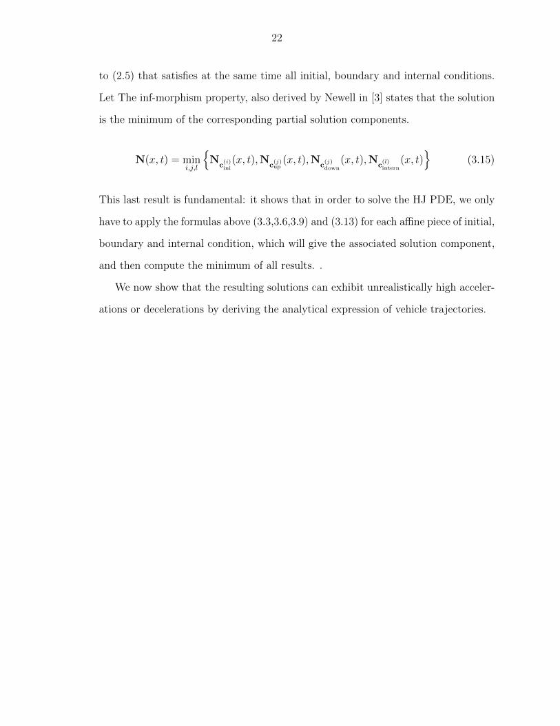
to (2.5) that satisfies at the same time all initial, boundary and internal conditions.

Let The inf-morphism property, also derived by Newell in [3] states that the solution

is the minimum of the corresponding partial solution components.

N(x, t) = mini,j,l

{N

c(i)ini

(x, t),Nc

(j)up

(x, t),Nc

(j)down

(x, t),Nc

(l)intern

(x, t)}

(3.15)

This last result is fundamental: it shows that in order to solve the HJ PDE, we only

have to apply the formulas above (3.3,3.6,3.9) and (3.13) for each affine piece of initial,

boundary and internal condition, which will give the associated solution component,

and then compute the minimum of all results. .

We now show that the resulting solutions can exhibit unrealistically high acceler-

ations or decelerations by deriving the analytical expression of vehicle trajectories.

23

Chapter 4

Analytical Derivation of Vehicle

Trajectories

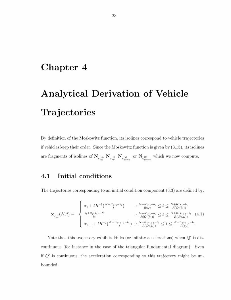
By definition of the Moskowitz function, its isolines correspond to vehicle trajectories

if vehicles keep their order. Since the Moskowitz function is given by (3.15), its isolines

are fragments of isolines of Nc

(i)ini

, Nc

(j)up

, Nc

(j)down

, or Nc

(l)intern

which we now compute.

4.1 Initial conditions

The trajectories corresponding to an initial condition component (3.3) are defined by:

xc

(i)ini

(N, t) =

xi + tR−1(N+Kixi−bi

t) : N+Kixi−bi

R(ω)≤ t ≤ N+Kixi−bi

R(Q′(ki))

bi+tQ(ki)−Nki

: N+Kixi−biR(Q′(ki))

≤ t ≤ N+Kixi+1−biR(Q′(ki))

xi+1 + tR−1(N+Kixi+1−bit

) : N+Kixi+1−biR(Q′(ki))

≤ t ≤ N+Kixi+1−biR(vf )

(4.1)

Note that this trajectory exhibits kinks (or infinite accelerations) when Q′ is dis-

continuous (for instance in the case of the triangular fundamental diagram). Even

if Q′ is continuous, the acceleration corresponding to this trajectory might be un-

bounded.

24

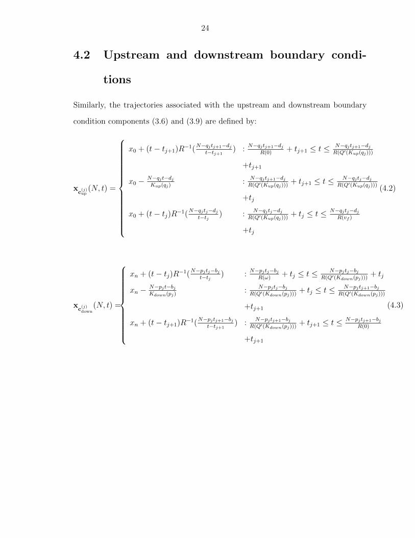
4.2 Upstream and downstream boundary condi-

tions

Similarly, the trajectories associated with the upstream and downstream boundary

condition components (3.6) and (3.9) are defined by:

xc

(j)up

(N, t) =

x0 + (t− tj+1)R−1(N−qjtj+1−dj

t−tj+1) :

N−qjtj+1−djR(0)

+ tj+1 ≤ t ≤ N−qjtj+1−djR(Q′(Kup(qj)))

+tj+1

x0 − N−qjt−djKup(qj)

:N−qjtj+1−djR(Q′(Kup(qj)))

+ tj+1 ≤ t ≤ N−qjtj−djR(Q′(Kup(qj)))

+tj

x0 + (t− tj)R−1(N−qjtj−dj

t−tj ) :N−qjtj−dj

R(Q′(Kup(qj)))+ tj ≤ t ≤ N−qjtj−dj

R(vf )

+tj

(4.2)

xc

(j)down

(N, t) =

xn + (t− tj)R−1(N−pjtj−bj

t−tj ) :N−pjtj−bj

R(ω)+ tj ≤ t ≤ N−pjtj−bj

R(Q′(Kdown(pj)))+ tj

xn − N−pjt−bjKdown(pj)

:N−pjtj−bj

R(Q′(Kdown(pj)))+ tj ≤ t ≤ N−pjtj+1−bj

R(Q′(Kdown(pj)))

+tj+1

xn + (t− tj+1)R−1(N−pjtj+1−bj

t−tj+1) :

N−pjtj+1−bjR(Q′(Kdown(pj)))

+ tj+1 ≤ t ≤ N−pjtj+1−bjR(0)

+tj+1

(4.3)

25

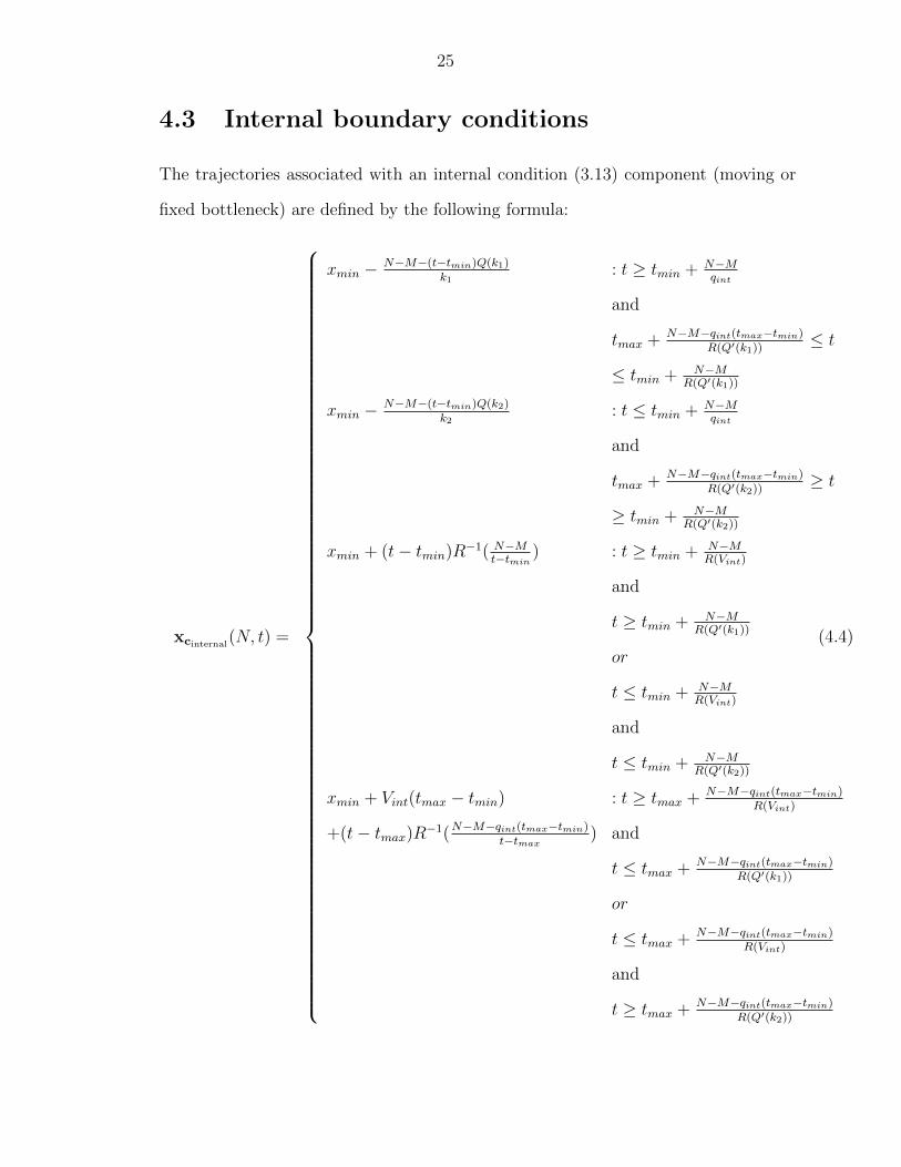
4.3 Internal boundary conditions

The trajectories associated with an internal condition (3.13) component (moving or

fixed bottleneck) are defined by the following formula:

xcinternal(N, t) =

xmin − N−M−(t−tmin)Q(k1)k1

: t ≥ tmin + N−Mqint

and

tmax + N−M−qint(tmax−tmin)R(Q′(k1))

≤ t

≤ tmin + N−MR(Q′(k1))

xmin − N−M−(t−tmin)Q(k2)k2

: t ≤ tmin + N−Mqint

and

tmax + N−M−qint(tmax−tmin)R(Q′(k2))

≥ t

≥ tmin + N−MR(Q′(k2))

xmin + (t− tmin)R−1( N−Mt−tmin

) : t ≥ tmin + N−MR(Vint)

and

t ≥ tmin + N−MR(Q′(k1))

or

t ≤ tmin + N−MR(Vint)

and

t ≤ tmin + N−MR(Q′(k2))

xmin + Vint(tmax − tmin) : t ≥ tmax + N−M−qint(tmax−tmin)R(Vint)

+(t− tmax)R−1(N−M−qint(tmax−tmin)t−tmax

) and

t ≤ tmax + N−M−qint(tmax−tmin)R(Q′(k1))

or

t ≤ tmax + N−M−qint(tmax−tmin)R(Vint)

and

t ≥ tmax + N−M−qint(tmax−tmin)R(Q′(k2))

(4.4)

26

As in the previous cases, the acceleration corresponding to these trajectories can be

unbounded or can exceed the physical capabilities of the vehicles.

27

Chapter 5

Definition of the Solution to the

Two Phase LWR Flow Model with

Bounded Acceleration

5.1 The two phase bounded acceleration-LWR traf-

fic flow model

The two phase bounded acceleration-LWR traffic flow model was introduced in [14],

and further extended in [7] for fixed and moving bottlenecks, where it was known

as the field bounded acceleration model. A numerical solver based on the Godunov

scheme is also derived in [7].

Defining the solution to the two phase model is complex. In [14], it requires

the computation of phase transition boundaries, which is very complex for general

problems involving moving bottlenecks. In [7], the solution is derived from the Go-

dunov scheme by modifying the fundamental diagram in the different areas of the

computational domain.

Instead, in this article we define the solution to the two phase bounded acceleration-

28

LWR problem in the Moskowitz space by the following implicit formula, which does

not require density-dependent modifications of the fundamental diagram nor the com-

putation of transition zones.

We first define the vehicle speed corresponding to the initial, boundary and inter-

nal condition components Nc(i) as follows:

vc(i)(t, x) =−∂N

c(i) (t,x)

∂t

∂Nc(i) (t,x)

∂x

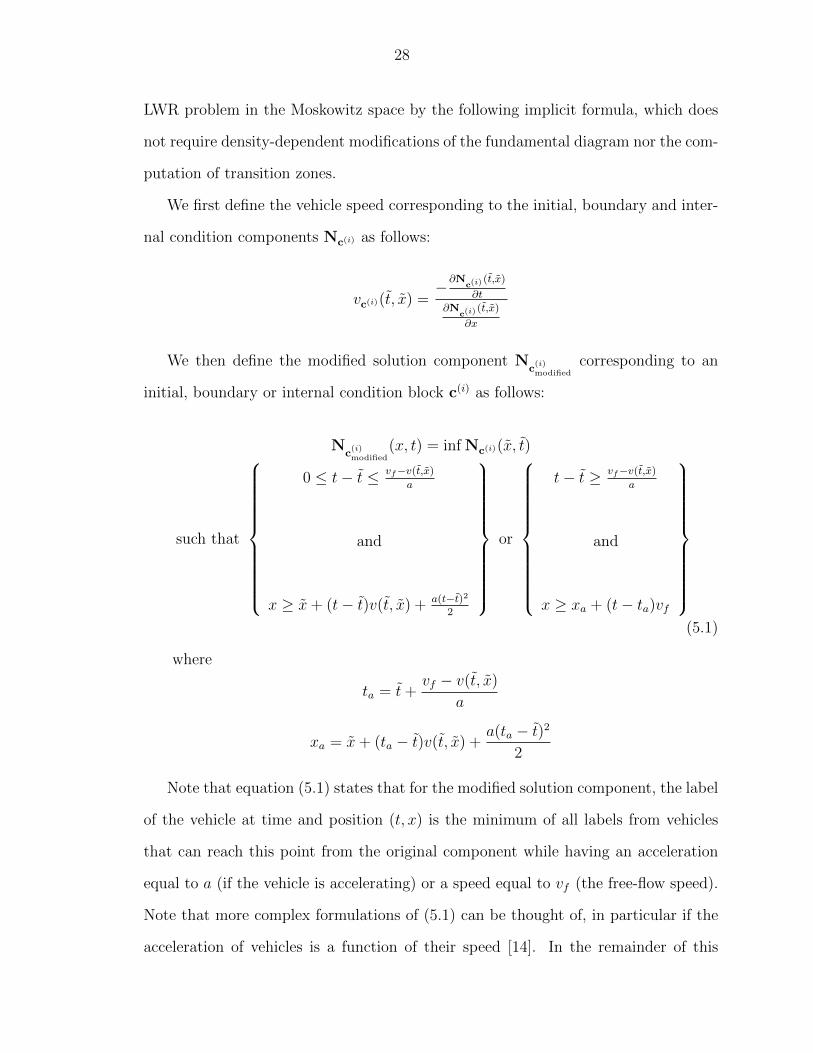
We then define the modified solution component Nc

(i)modified

corresponding to an

initial, boundary or internal condition block c(i) as follows:

Nc

(i)modified

(x, t) = inf Nc(i)(x, t)

such that

0 ≤ t− t ≤ vf−v(t,x)

a

and

x ≥ x+ (t− t)v(t, x) + a(t−t)2

2

or

t− t ≥ vf−v(t,x)

a

and

x ≥ xa + (t− ta)vf

(5.1)

where

ta = t+vf − v(t, x)

a

xa = x+ (ta − t)v(t, x) +a(ta − t)2

2

Note that equation (5.1) states that for the modified solution component, the label

of the vehicle at time and position (t, x) is the minimum of all labels from vehicles

that can reach this point from the original component while having an acceleration

equal to a (if the vehicle is accelerating) or a speed equal to vf (the free-flow speed).

Note that more complex formulations of (5.1) can be thought of, in particular if the

acceleration of vehicles is a function of their speed [14]. In the remainder of this

29

article, we will assume that the acceleration of all vehicles is upper bounded by a,

irrespective of their current speed as in (5.1).

Given the definition (5.1), the solution Nmodified(·, ·) to the hybrid two phase LWR-

bounded acceleration model is defined by:

Nmodified(x, t) = mini∈I

Nc

(i)modified

(x, t) (5.2)

Note that the solution to the hybrid two phase LWR-bounded acceleration model (5.2)

shares the same solution structure as the solution to the HJ PDE (3.15) investigated

in [21]. Indeed, the only difference between both formulations is in the definition of

the partial solution components (5.1).

5.2 Properties of the solutions

The solution (5.2) and the partial solution components defined by (5.1) have impor-

tant properties, which we now outline.

5.2.1 Inf property

Let c(i) represent an initial, boundary or internal condition block (3.2), (3.5), (3.8)

or (2.12), Nc(i) be the corresponding solution component, and Nc

(i)modified

be the modi-

fied solution component as in (5.1). We have that Nc

(i)modified

≤ Nc(i) pointwise.

Proof — The proof of this fact follows the fact that (x, t) = (x, t) is always in the

feasible set of (5.1). �

30

5.2.2 Structure of the resulting solutions

The solution Nmodified(·, ·) to the hybrid two phase traffic flow model satisfies the

following property:

(i) Either Nmodified(x, t) = Nc(i)(x, t)

(ii) Or

∃t, x s.t. t < t and (x ≥ x+ (t− t)v(t, x) + a(t−t)2

2or x ≥ xa + (t− ta)vf )

and Nmodified(t, x) = Nmodified(t, x)

(5.3)

Proof — Let us fix (x, t) ∈ [ξ, χ]× R+, and consider the feasible set S of (5.1). We

always have that (x, t) ∈ S. Two situations can arise:

1. If (x, t) minimizes the objective function of (5.1), then Nmodified(x, t) = Nc(i)(x, t),

that is, (5.3) (i)

2. If (x, t) 6= (x, t) minimizes the objective function of (5.1), we have (5.3) (ii)

�

Note that (5.3) is very important: if locally Nmodified(x, t) = Nc(i)(x, t), we have

that Nmodified satisfies (2.5) locally, using the tangential properties of the capture basin

(see [30]) for the construction of the solutions to the HJ PDE using capture basins).

However, if (5.3) is satisfied, then Nmodified(x, t) describes locally the evolution of

a vehicle having a constant acceleration up to its maximal velocity vf , and then a

constant velocity.

5.2.3 Solution structure

The solution to the mixed initial-boundary-internal conditions problem (5.2) also

shares the property (5.3), as it is the minimum of a finite number of functions sat-

isfying (5.3). Though no framework for describing hybridness in partial differential

31

equations exists, the solutions to the two phase flow model have an hybrid structure:

they are either solutions to the HJ PDE (2.5) derived from the LWR PDE (2.2), or

represent trajectories of vehicles with bounded acceleration.

32

Chapter 6

Analytical Derivation of the

Modified Solution Components for

the Triangular Fundamental

Diagram

The solution components (5.1) are defined semi-explicitly as a minimization problem

in general. However, if the fundamental diagram Q(·) is known explicitly, these solu-

tion components may be computed explicitly. We now derive the explicit expression

of the solution components associated with affine initial, upstream and downstream

boundary, or internal conditions blocks, for a triangular fundamental diagram Q de-

fined by the following expression.

Q(k) =

vfk : x ∈ [0, kc]

w(k − κ) : x ∈ [kc, κ](6.1)

We also have by continuity of Q(k) kc that kc = −w κvf−w . The triangular funda-

mental diagram is widely used in the literature [16] since it is particularly simple and

33

robust.

6.1 Initial condition

6.1.1 Free-flow initial condition

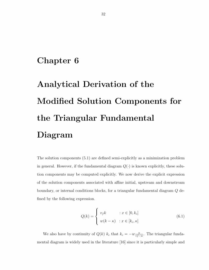
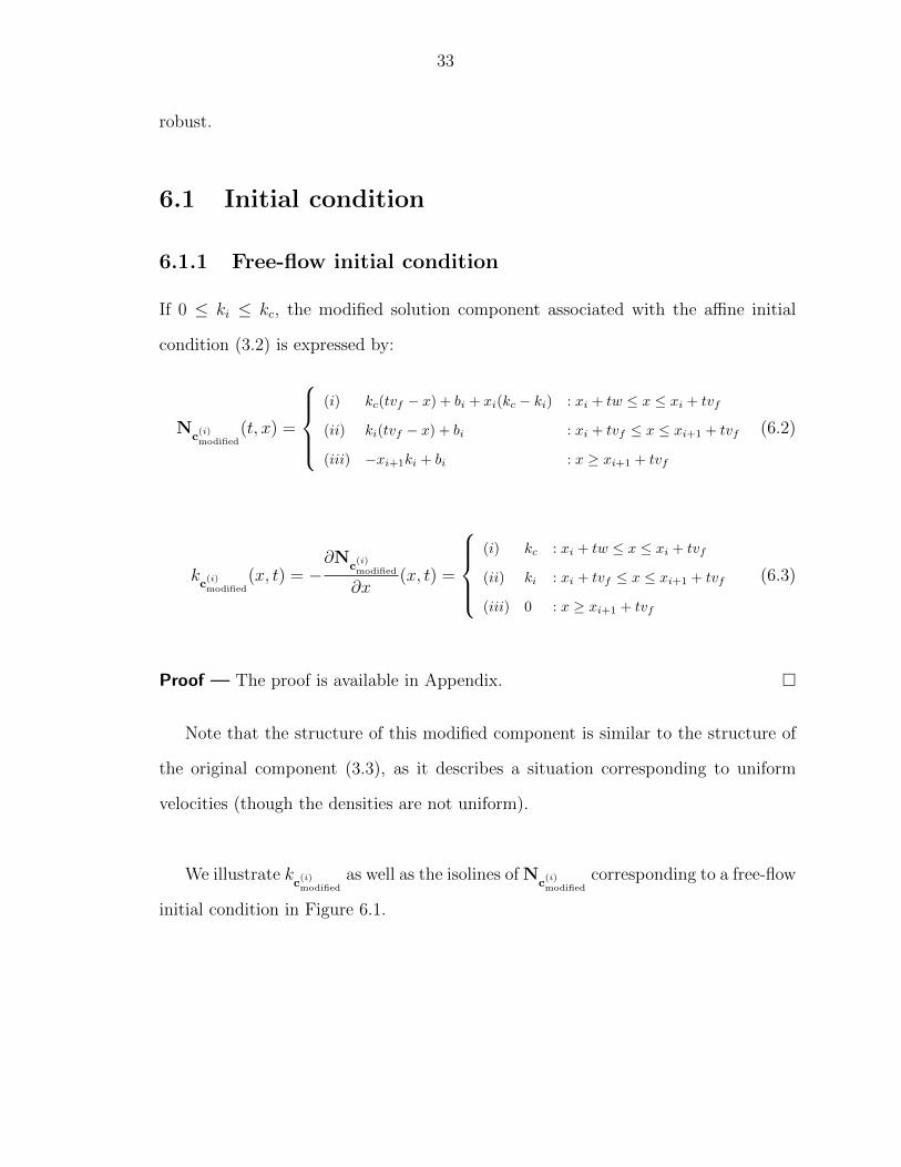
If 0 ≤ ki ≤ kc, the modified solution component associated with the affine initial

condition (3.2) is expressed by:

Nc

(i)modified

(t, x) =

(i) kc(tvf − x) + bi + xi(kc − ki) : xi + tw ≤ x ≤ xi + tvf

(ii) ki(tvf − x) + bi : xi + tvf ≤ x ≤ xi+1 + tvf

(iii) −xi+1ki + bi : x ≥ xi+1 + tvf

(6.2)

kc

(i)modified

(x, t) = −∂N

c(i)modified

∂x(x, t) =

(i) kc : xi + tw ≤ x ≤ xi + tvf

(ii) ki : xi + tvf ≤ x ≤ xi+1 + tvf

(iii) 0 : x ≥ xi+1 + tvf

(6.3)

Proof — The proof is available in Appendix. �

Note that the structure of this modified component is similar to the structure of

the original component (3.3), as it describes a situation corresponding to uniform

velocities (though the densities are not uniform).

We illustrate kc

(i)modified

as well as the isolines of Nc

(i)modified

corresponding to a free-flow

initial condition in Figure 6.1.

34

Figure 6.1: Density map kc

(i)modified

corresponding to an uncongested initial condition,

for a triangular fundamental diagram.

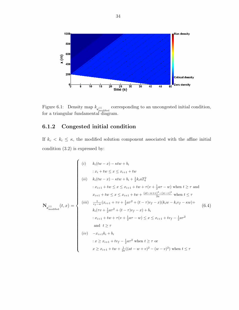
6.1.2 Congested initial condition

If kc < ki ≤ κ, the modified solution component associated with the affine initial


Nc

(i)modified

(t, x) =

(i) ki(tw − x)− κtw + bi

: xi + tw ≤ x ≤ xi+1 + tw

(ii) ki(tw − x)− κtw + bi +12kiaT

24

: xi+1 + tw ≤ x ≤ xi+1 + tw + τ(v + 12aτ − w) when t ≥ τ and

xi+1 + tw ≤ x ≤ xi+1 + tw + (at−w+v)2−(w−v)22a when t ≤ τ

(iii) 1vf−w (xi+1 + τv + 1

2aτ2 + (t− τ)vf − x)(kiw − kivf − κw)+

ki(τv +12aτ

2 + (t− τ)vf − x) + bi

: xi+1 + tw + τ(v + 12aτ − w) ≤ x ≤ xi+1 + tvf − 1

2aτ2

and t ≥ τ

(iv) −xi+1ki + bi

: x ≥ xi+1 + tvf − 12aτ

2 when t ≥ τ or

x ≥ xi+1 + tw + 12a ((at− w + v)2 − (w − v)2) when t ≤ τ

(6.4)

35

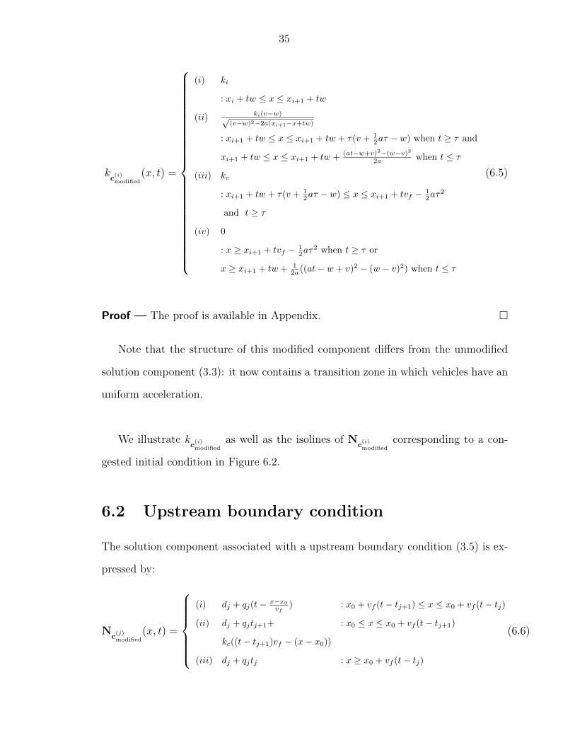
kc

(i)modified

(x, t) =

(i) ki

: xi + tw ≤ x ≤ xi+1 + tw

(ii) ki(v−w)√(v−w)2−2a(xi+1−x+tw)


xi+1 + tw ≤ x ≤ xi+1 + tw + (at−w+v)2−(w−v)22a when t ≤ τ

(iii) kc


2aτ2

and t ≥ τ

(iv) 0

: x ≥ xi+1 + tvf − 12aτ

2 when t ≥ τ or

x ≥ xi+1 + tw + 12a ((at− w + v)2 − (w − v)2) when t ≤ τ

(6.5)

Proof — The proof is available in Appendix. �

Note that the structure of this modified component differs from the unmodified

solution component (3.3): it now contains a transition zone in which vehicles have an

uniform acceleration.

We illustrate kc

(i)modified


(i)modified

corresponding to a con-

gested initial condition in Figure 6.2.

6.2 Upstream boundary condition

The solution component associated with a upstream boundary condition (3.5) is ex-

pressed by:

Nc

(j)modified

(x, t) =

(i) dj + qj(t− x−x0

vf) : x0 + vf (t− tj+1) ≤ x ≤ x0 + vf (t− tj)

(ii) dj + qjtj+1+ : x0 ≤ x ≤ x0 + vf (t− tj+1)

kc((t− tj+1)vf − (x− x0))

(iii) dj + qjtj : x ≥ x0 + vf (t− tj)

(6.6)

36


(i)modified

corresponding to a congested initial condition, for

a triangular fundamental diagram.

kc

(j)modified

(x, t) = −∂N

c(j)modified

∂x(x, t) =

(i)

qjvf

: x0 + vf (t− tj+1) ≤ x ≤ x0 + vf (t− tj)

(ii) kc : x0 ≤ x ≤ x0 + vf (t− tj+1)

(iii) 0 : x ≥ x0 + vf (t− tj)

(6.7)

Proof — The proof is similar to the initial condition case. �

Note that the structure of this modified component is very similar to the unmod-

ified component (3.6), as it describes a situation corresponding to uniform velocities

(though the densities are not uniform).

We illustrate kc

(i)modified


(j)modified

corresponding to an up-

stream boundary condition in Figure 6.3.

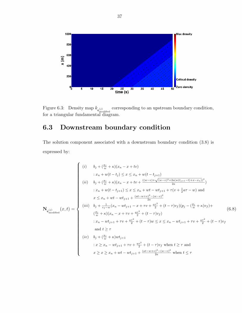
37


(j)modified

corresponding to an upstream boundary condition,

for a triangular fundamental diagram.

6.3 Downstream boundary condition

The solution component associated with a downstream boundary condition (3.8) is

expressed by:

Nc

(j)modified

(x, t) =

(i) bj + (pjw + κ)(xn − x+ tv)

: xn + w(t− tj) ≤ x ≤ xn + w(t− tj+1)

(ii) bj + (pjw + κ)(xn − x+ tv +

((w−v)+√

(w−v)2+2a(w(tj+1−t)+x−xn))2

2a )

: xn + w(t− tj+1) ≤ x ≤ xn + wt− wtj+1 + τ(v + 12aτ − w) and

x ≤ xn + wt− wtj+1 +(at−w+v)2−(w−v)2

2a

(iii) bj +1

vf−w (xn − wtj+1 − x+ τv + aτ2

2 + (t− τ)vf )(pj − (pjw + κ)vf )+

(pjw + κ)(xn − x+ τv + aτ2

2 + (t− τ)vf )

: xn − wtj+1 + τv + aτ2

2 + (t− τ)w ≤ x ≤ xn − wtj+1 + τv + aτ2

2 + (t− τ)vf

and t ≥ τ

(iv) bj + (pjw + κ)wtj+1

: x ≥ xn − wtj+1 + τv + aτ2

2 + (t− τ)vf when t ≥ τ and

x ≥ x ≥ xn + wt− wtj+1 +(at−w+v)2−(w−v)2

2a when t ≤ τ

(6.8)

38

kc

(j)modified

(x, t) =

(i)pjw + κ

: xn + w(t− tj) ≤ x ≤ xn + w(t− tj+1)

(ii)(pjw +κ)(v−w)√

(w−v)2+2a(w(tj+1−t)+x−xn)

: xn + w(t− tj+1) ≤ x ≤ xn + wt− wtj+1 + τ(v + 12aτ − w) and

x ≤ xn + wt− wtj+1 +(at−w+v)2−(w−v)2

2a

(iii) kc

: xn − wtj+1 + τv + aτ2

2 + (t− τ)w ≤ x ≤ xn − wtj+1 + τv + aτ2

2 + (t− τ)vf

and t ≥ τ

(iv) 0

: x ≥ xn − wtj+1 + τv + aτ2

2 + (t− τ)vf when t ≥ τ and

x ≥ x ≥ xn + wt− wtj+1 +(at−w+v)2−(w−v)2

2a when t ≤ τ

(6.9)



solution component (3.9): it now contains a transition zone in which vehicles have an

uniform acceleration.

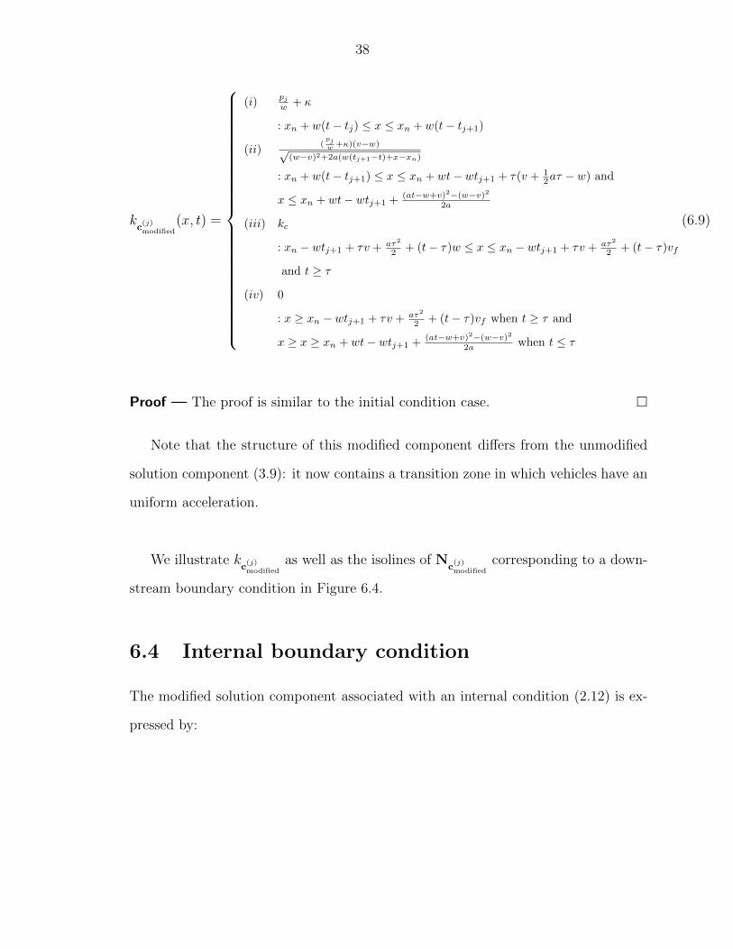
We illustrate kc

(j)modified


(j)modified

corresponding to a down-

stream boundary condition in Figure 6.4.

6.4 Internal boundary condition

The modified solution component associated with an internal condition (2.12) is ex-

pressed by:

39


(j)modified

corresponding to a downstream boundary condi-

tion, for a triangular fundamental diagram.

Nc

(l)modified

(x, t) =

(i) M (l) − w(k2 − κ)t(l)min + (x(l)min − x) + tv)k2

: x 6 x(l)min + V(l)intern(t− t

(l)min) and

x > x(l)min + w(t− t(l)min) and

x 6 x(l)max + w(t− t(l)max)

(ii) M (l) − w(k2 − κ)t(l)min + (x(l)min − x+ tv)k2 +

k2a2 T 2

4

: x > x(l)max + w(t− t(l)max) and

x 6 (aτ−w+v)2−(w−v)22a + x

(l)max + w(t− t(l)max) and

x 6 a(t−t(l)max)2

2 + v(t− t(l)max) + x(l)max and

t > t(l)max +V

(l)intern−v

a

(iii) M (l) − w(k2 − κ)t(l)min + (x(l)min − x+ tv)k2 +

k2a2 T 2

2

: x > − (V(l)intern−v)

2

2a + x(l)min + V

(l)intern(t− t

(l)min) and

x 6 (aτ−w+v)2−(w−v)22a + x


x 6 a(t−t(l)min)2

2 + v(t− t(l)min) + x(l)min and

t > t(l)min +V

(l)intern−v

a

x 6 (aτ−V (l)intern+v)

2−(V(l)intern−v)

2

2a + x(l)min+

V(l)intern(t− t

(l)min) and

x > x(l)min + V(l)intern(t− t

(l)min)

x > a(t−t(l)max)2

2 + v(t− t(l)max) + x(l)max,

t > t(l)max +V

(l)intern−v

a or t 6 t(l)max +V

(l)intern−v

a

(6.10)

40

Nc

(l)modified

(x, t) =

(iv) w(k2 − κ)(t1 − t(l)min)− vfk2t1 + (x(l)min − x+ τv + aτ2

2 + (t− τ)vf )k2 +M (l)

: x > x(l)min − V(l)internt

(l)min + τv + aτ2

2 + (t− τ)V (l)intern and

x > 1

w−V (l)intern

((w − V (l)intern)(τv +

aτ2

2 + (t− τ)vf )+

(vf − V (l)intern)(xmax − wt

(l)max)− (vf − w)(xmin − V (l)

internt(l)min) and

x 6 x(l)min − vf t(l)min + τv + aτ2

2 + (t− τ)vf and

t > τ

(v) w(k2 − κ)(t2 − t(l)min)− vfk2t2 + (x(l)min − x+ τv + aτ2

2 + (t− τ)vf )k2 +M (l)

: x > xmax − wtmax + τv + aτ2

2 + (t− τ)w and

x 6 xmax − wtmax + τv + aτ2

2 + (t− τ)vf and

x 6 1

w−V (l)intern


aτ2

2 + (t− τ)vf )+



internt(l)min) and

t > τ

(vi) M (l)

: x > a(t−t(l)min)2


x 6 x(l)min − V(l)internt

(l)min + τv + aτ2


t > t(l)min

or

x > x(l)min − vf t(l)min + τv + aτ2

2 + (t− τ)vf and

x > x(l)min − V(l)internt

(l)min + τv + aτ2


t > t(minl)

(6.11)

kc

(l)modified

(x, t) =

(i) k2

: x 6 x(l)min + V(l)intern(t− t

(l)min) and

x > x(l)min + w(t− t(l)min) and

x 6 x(l)max + w(t− t(l)max)

(ii) k2(v−w)√(v−w)2+2a(x−x(l)

max−w(t−t(l)max))

: x > x(l)max + w(t− t(l)max) and

x 6 (aτ−w+v)2−(w−v)22a + x


x 6 a(t−t(l)max)2

2 + v(t− t(l)max) + x(l)max and

t > t(l)max +V

(l)intern−v

a

(6.12)

41

kc

(l)modified

(x, t) =

(iii)k2(V

(l)intern−w)√

(V(l)intern−w)2+2a(x−x(l)

min−V(l)intern(t−t

(l)min))

: x > − (V(l)intern−v)

2

2a + x(l)min + V

(l)intern(t− t

(l)min) and

x 6 (aτ−w+v)2−(w−v)22a + x


x 6 a(t−t(l)min)2


t > t(l)min +V

(l)intern−v

a

x 6 (aτ−V (l)intern+v)

2−(V(l)intern−v)

2

2a + x(l)min + V

(l)intern(t− t

(l)min) and

x > x(l)min + V(l)intern(t− t

(l)min)

x > a(t−t(l)max)2

2 + v(t− t(l)max) + x(l)max,

t > t(l)max +V

(l)intern−v

a or t 6 t(l)max +V

(l)intern−v

a

(iv) k2 +w(k2−κ)−vfk2vf−V (l)

intern

: x > x(l)min − V(l)internt

(l)min + τv + aτ2


x > 1

w−V (l)intern


aτ2

2 + (t− τ)vf )+



internt(l)min) and

x 6 x(l)min − vf t(l)min + τv + aτ2

2 + (t− τ)vf and

t > τ

(v) k2 +w(k2−κ)−vfk2

vf−w

: x > xmax − wtmax + τv + aτ2

2 + (t− τ)w and

x 6 xmax − wtmax + τv + aτ2

2 + (t− τ)vf and

x 6 1

w−V (l)intern


aτ2

2 + (t− τ)vf )+



internt(l)min) and

t > τ

(vi) 0

: x > a(t−t(l)min)2


x 6 x(l)min − V(l)internt

(l)min + τv + aτ2


t > t(l)min

or

x > x(l)min − vf t(l)min + τv + aτ2

2 + (t− τ)vf and

x > x(l)min − V(l)internt

(l)min + τv + aτ2


t > t(l)min

(6.13)

42

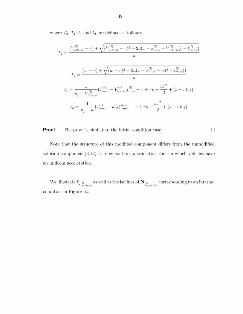
where T2, T4, t1 and t2 are defined as follows:

T2 =(V

(l)intern − v) +

√(V

(l)intern − v)2 + 2a(x− x(l)

min − V(l)intern(t− t(l)min))

a

T4 =(w − v) +

√(w − v)2 + 2a(x− x(l)

max − w(t− t(l)max))a

t1 =1

vf − V (l)intern

(x(l)min − V

(l)internt

(l)min − x+ τv +

aτ 2

2+ (t− τ)vf )

t2 =1

vf − w(x(l)

max − w(l)t(l)max − x+ τv +aτ 2

2+ (t− τ)vf )



solution component (3.13): it now contains a transition zone in which vehicles have

an uniform acceleration.

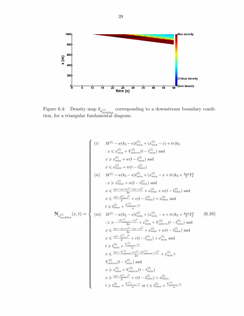
We illustrate kc

(l)modified


(l)modified

corresponding to an internal

condition in Figure 6.5.

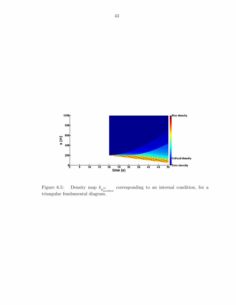
43


(l)modified

corresponding to an internal condition, for a

triangular fundamental diagram.

44

Chapter 7

Implementation

7.1 Algorithm structure

Given the derivations of the modified component solutions associated with the ini-

tial, boundary and internal conditions, one can build a numerical scheme for solving

the hybrid two phase LWR-bounded acceleration model semi-analytically with a low

computational cost, as in [21].

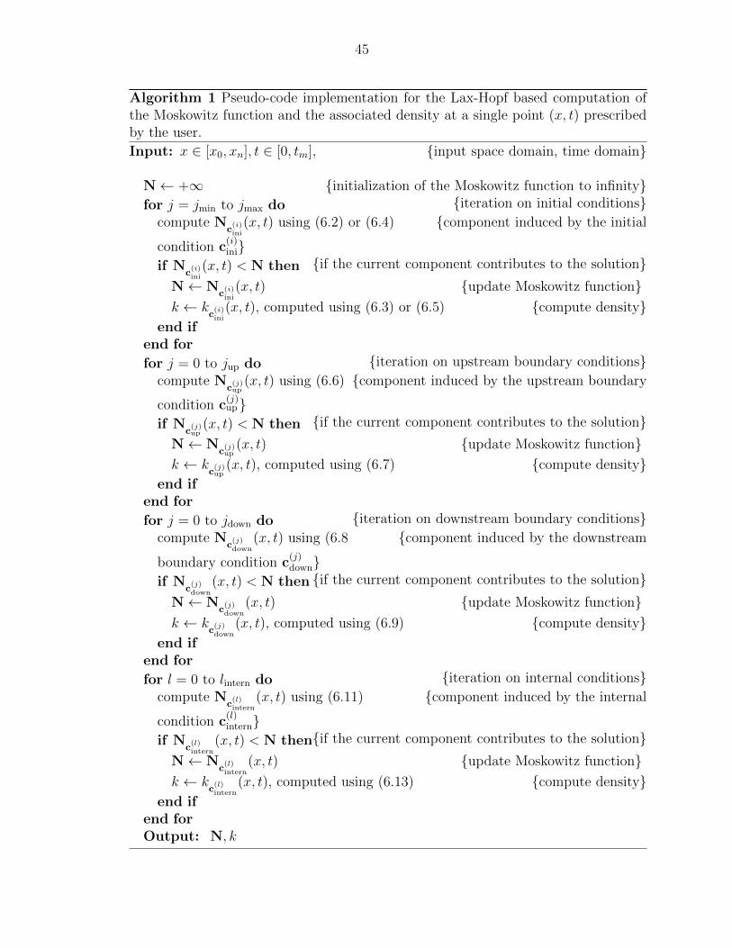
The proposed numerical scheme is based on the inf-morphism property (3.15). It

is based on the minimization of analytic formulas, and is thus guaranteed to be exact.

45

Algorithm 1 Pseudo-code implementation for the Lax-Hopf based computation ofthe Moskowitz function and the associated density at a single point (x, t) prescribedby the user.

Input: x ∈ [x0, xn], t ∈ [0, tm], {input space domain, time domain}

N← +∞ {initialization of the Moskowitz function to infinity}{iteration on initial conditions}for j = jmin to jmax do

compute Nc

(i)ini

(x, t) using (6.2) or (6.4) {component induced by the initial

condition c(i)ini}

{if the current component contributes to the solution}if Nc

(i)ini

(x, t) < N then

N← Nc

(i)ini

(x, t) {update Moskowitz function}k ← k

c(i)ini

(x, t), computed using (6.3) or (6.5) {compute density}end if

end for{iteration on upstream boundary conditions}for j = 0 to jup do

compute Nc

(j)up

(x, t) using (6.6) {component induced by the upstream boundary

condition c(j)up}


(j)up

(x, t) < N then

N← Nc

(j)up


c(j)up

(x, t), computed using (6.7) {compute density}end if

end for{iteration on downstream boundary conditions}for j = 0 to jdown do

compute Nc

(j)down

(x, t) using (6.8 {component induced by the downstream

boundary condition c(j)down}{if the current component contributes to the solution}if N

c(j)down

(x, t) < N then

N← Nc

(j)down


c(j)down


end for{iteration on internal conditions}for l = 0 to lintern do

compute Nc

(l)intern

(x, t) using (6.11) {component induced by the internal

condition c(l)intern}


(l)intern

(x, t) < N then

N← Nc

(l)intern


c(l)intern


end forOutput: N, k

46

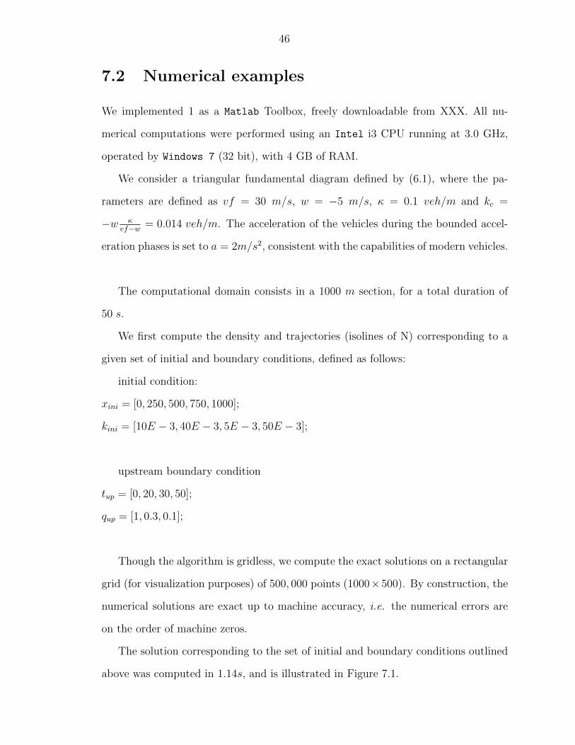
7.2 Numerical examples

We implemented 1 as a Matlab Toolbox, freely downloadable from XXX. All nu-

merical computations were performed using an Intel i3 CPU running at 3.0 GHz,

operated by Windows 7 (32 bit), with 4 GB of RAM.

We consider a triangular fundamental diagram defined by (6.1), where the pa-

rameters are defined as vf = 30 m/s, w = −5 m/s, κ = 0.1 veh/m and kc =

−w κvf−w = 0.014 veh/m. The acceleration of the vehicles during the bounded accel-

eration phases is set to a = 2m/s2, consistent with the capabilities of modern vehicles.

The computational domain consists in a 1000 m section, for a total duration of

50 s.

We first compute the density and trajectories (isolines of N) corresponding to a

given set of initial and boundary conditions, defined as follows:

initial condition:

xini = [0, 250, 500, 750, 1000];

kini = [10E − 3, 40E − 3, 5E − 3, 50E − 3];

upstream boundary condition

tup = [0, 20, 30, 50];

qup = [1, 0.3, 0.1];

Though the algorithm is gridless, we compute the exact solutions on a rectangular

grid (for visualization purposes) of 500, 000 points (1000×500). By construction, the

numerical solutions are exact up to machine accuracy, i.e. the numerical errors are

on the order of machine zeros.

The solution corresponding to the set of initial and boundary conditions outlined

above was computed in 1.14s, and is illustrated in Figure 7.1.

47

Figure 7.1: Density map and vehicle trajectories corresponding to a set of initialand upstream boundary conditions.

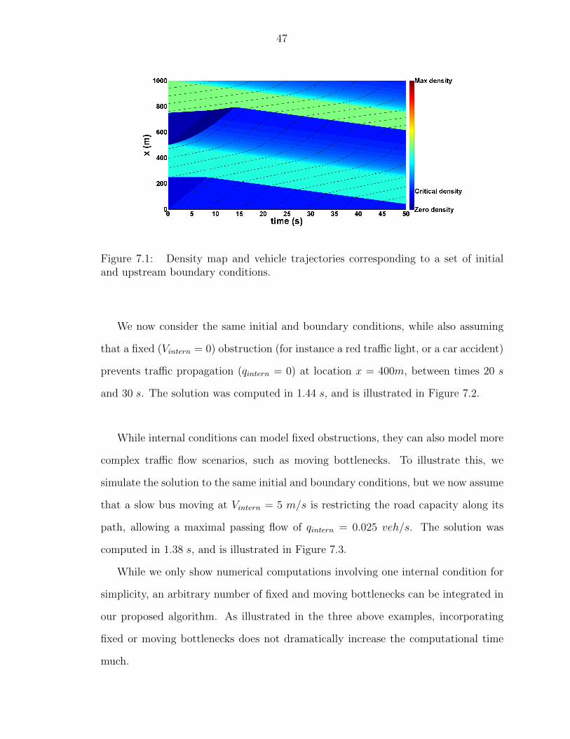
We now consider the same initial and boundary conditions, while also assuming

that a fixed (Vintern = 0) obstruction (for instance a red traffic light, or a car accident)

prevents traffic propagation (qintern = 0) at location x = 400m, between times 20 s

and 30 s. The solution was computed in 1.44 s, and is illustrated in Figure 7.2.

While internal conditions can model fixed obstructions, they can also model more

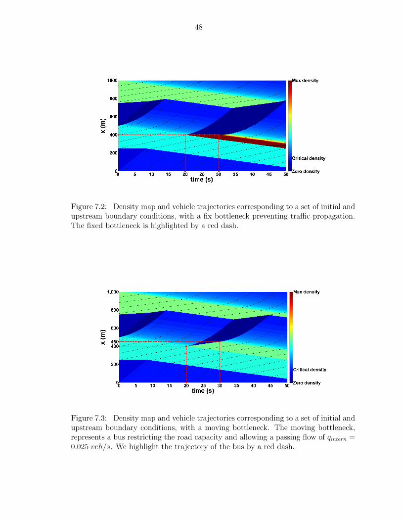
complex traffic flow scenarios, such as moving bottlenecks. To illustrate this, we

simulate the solution to the same initial and boundary conditions, but we now assume

that a slow bus moving at Vintern = 5 m/s is restricting the road capacity along its

path, allowing a maximal passing flow of qintern = 0.025 veh/s. The solution was

computed in 1.38 s, and is illustrated in Figure 7.3.

While we only show numerical computations involving one internal condition for

simplicity, an arbitrary number of fixed and moving bottlenecks can be integrated in

our proposed algorithm. As illustrated in the three above examples, incorporating

fixed or moving bottlenecks does not dramatically increase the computational time

much.

48

Figure 7.2: Density map and vehicle trajectories corresponding to a set of initial andupstream boundary conditions, with a fix bottleneck preventing traffic propagation.The fixed bottleneck is highlighted by a red dash.

Figure 7.3: Density map and vehicle trajectories corresponding to a set of initial andupstream boundary conditions, with a moving bottleneck. The moving bottleneck,represents a bus restricting the road capacity and allowing a passing flow of qintern =0.025 veh/s. We highlight the trajectory of the bus by a red dash.

49

7.3 Benefits of a grid-free and exact method

The fact that the proposed numerical scheme is both exact and gridless is very im-

portant for solving practical problems involving the kinematic effects of vehicles on

traffic flow propagation. For instance, dealing with the effects of traffic flow (pollu-

tion, energy consumption, noise...) often requires the coupling between traffic flow

propagation models and vehicle property models (for instance the energy consumption

of the vehicle as a function of its target path). Optimizing these effects (for instance

minimizing pollution of a bus driving through traffic) thus requires the computation

of an optimal single vehicle trajectory, which is itself a function of the surrounding

traffic. Most algorithms compute these trajectories iteratively, and thus any error

of the numerical traffic solver is propagated through the iterations, leading to poor

overall accuracy. Since the algorithm described in this article is exact, it does not

add any uncertainty to the results.

The fact that the algorithm is grid-free also allows for a faster search over all

possible vehicle trajectories for single vehicle trajectory optimization problems.

50

Chapter 8

Conclusion

This article presents a new semi analytical expression for the solutions to the Lighthill-

Whitham-Richards traffic flow model with bounded vehicle acceleration. Based on

this semi-analytical expression, we compute the analytical solution component blocks

associated with the triangular fundamental diagram. These analytical solution blocks

allow us to construct the solution to the modified traffic flow model as a finite min-

imization of functions. The resulting numerical scheme is both grid-free and exact,

which are very favorable characteristics when dealing with optimization problems in-

volving the coupling between the modified LWR model and vehicle models. We then

use the algorithm to compute the solutions to various problems involving fixed and

moving bottlenecks of increased complexity.

Future work will deal with the extension of this algorithm to networks, as bounded

accelerations frequently occur in junctions, whenever congestion occurs because of

capacity restriction. Another important avenue is the development of an hybrid

model based on the Lighthill-Whitham-Richards traffic flow model with both bounded

acceleration and deceleration, which is to date an open problem.

51

REFERENCES

[1] M. J. Lighthill and G. B. Whitham, “On kinematic waves. II. A theory of

traffic flow on long crowded roads,” Proceedings of the Royal Society of London,

vol. 229, no. 1178, pp. 317–345, 1956.

[2] P. I. Richards, “Shock waves on the highway,” Operations Research, vol. 4,

no. 1, pp. 42–51, 1956.

[3] G. F. Newell, “A simplified theory of kinematic waves in highway traffic, Part

(I), (II) and (III),” Transporation Research B, vol. 27B, no. 4, pp. 281–313, 1993.

[4] N. Geroliminis and C. F. Daganzo, “Existence of urban-scale macroscopic

fundamental diagrams: Some experimental findings,” Transportation Research

Part B: Methodological, vol. 42, no. 9, pp. 759–770, 2008.

[5] R. Ansorge, “What does the entropy condition mean in traffic flow theory?”

Transportation Research, vol. 24B, no. 2, pp. 133–143, 1990.

[6] M. Bardi and I. Capuzzo-Dolcetta, Viscosity Solutions of Hamilton-Jacobi-

Bellman Equations. Boston, MA: Birkhauser, 1997.

[7] L. Leclercq, “Bounded acceleration close to fixed and moving bottlenecks,”

Transportation research. Part B: methodological, vol. 41, no. 3, pp. 309–319,

2007.

[8] J. A. Laval and C. F. Daganzo, “Lane-changing in traffic streams,” Trans-

portation Research Part B: Methodological, vol. 40, no. 3, pp. 251–264, 2006.

52

[9] J. P. Lebacque, “Two-phase bounded-acceleration traffic flow model: analyti-

cal solutions and applications,” Transportation Research Record: Journal of the

Transportation Research Board, vol. 1852, no. -1, pp. 220–230, 2003.

[10] L. Leclercq, J. A. Laval, and N. Chiabaut, “Capacity drops at merges: An

endogenous model,” Transportation Research Part B: Methodological, 2011.

[11] F. Giorgi, L. Leclercq, and J. B. Lesort, “A traffic flow model for urban

traffic analysis: extensions of the lwr model for urban and environmental appli-

cations,” in Proceedings of the 15th International Symposium on Transportation

and Traffic Theory, 2002, pp. 393–416.

[12] A. Aw and M. Rascle, “Resurrection of “second order” models of traffic flow,”

SIAM Journal of Applied Mathematics, vol. 60, no. 3, pp. 916–938, 2000.

[13] S. Blandin, D. Work, P. Goatin, B. Piccoli, A. Bayen et al., “A general

phase transition model for vehicular traffic,” SIAM Journal on Applied Mathe-

matics, vol. 71, no. 1, pp. 107–127, 2011.

[14] J. P. Lebacque, “A two phase extension of the LWR model based on the bound-

edness of traffic acceleration,” in Transportation and Traffic Theory in the 21st

Century. Proceedings of the 15th International Symposium on Transportation

and Traffic Theory, 2002.

[15] S. K. Godunov, “A difference method for numerical calculation of discontinuous

solutions of the equations of hydrodynamics,” Math. Sbornik, vol. 47, pp. 271–

306, 1959.

[16] C. Daganzo, “The cell transmission model: a dynamic representation of high-

way traffic consistent with the hydrodynamic theory,” Transportation Research,

vol. 28B, no. 4, pp. 269–287, 1994.

[17] ——, “The cell transmission model, part II: network traffic,” Transportation

Research, vol. 29B, no. 2, pp. 79–93, 1995.

53

[18] V. Henn, “A wave-based resolution scheme for the hydrodynamic LWR traffic

flow model,” in Proceedings of the Workshop on Traffic and Granular Flow 03,

B. S. W. Hoogendoorn, Luding, Ed., Amsterdam, 2003, pp. 105–124.

[19] C. G. Claudel and A. M. Bayen, “Lax-Hopf based incorporation of in-

ternal boundary conditions into Hamilton-Jacobi equation. Part I: theory,”

IEEE Transactions on Automatic Control, vol. 55, no. 5, pp. 1142–1157, 2010,

doi:10.1109/TAC.2010.2041976.

[20] ——, “Lax-Hopf based incorporation of internal boundary conditions into

Hamilton-Jacobi equation. Part II: Computational methods,” IEEE Trans-

actions on Automatic Control, vol. 55, no. 5, pp. 1158–1174, 2010,

doi:10.1109/TAC.2010.2045439.

[21] P. E. Mazare, A. Dehwah, C. G. Claudel, and A. M. Bayen, “Analyti-

cal and grid-free solutions to the lighthill-whitham-richards traffic flow model,”

Transportation Research Part B: Analytical., vol. 45, no. 10, pp. 1727–1748, 2011.

[22] M. Garavello and B. Piccolli, Traffic flow on networks. Springfield, MO:

American Institute of Mathematical Sciences, 2006.

[23] B. D. Greenshields, “A study of traffic capacity,” Proc. Highway Res. Board,

vol. 14, pp. 448–477, 1935.

[24] C. F. Daganzo, “On the variational theory of traffic flow: well-posedness, du-

ality and applications,” Networks and heterogeneous media, vol. 1, pp. 601–619,

2006.

[25] K. Moskowitz, “Discussion of ‘freeway level of service as influenced by volume

and capacity characteristics’ by D.R. Drew and C. J. Keese,” Highway Research

Record, vol. 99, pp. 43–44, 1965.

[26] C. F. Daganzo, “A variational formulation of kinematic waves: basic theory

and complex boundary conditions,” Transporation Research B, vol. 39B, no. 2,

pp. 187–196, 2005.

54

[27] Y. Makigami, G. F. Newell, and R. Rothery, “Three-dimensional represen-

tation of traffic flow,” Transportation Science, vol. 5, no. 3, pp. 303–313, Aug

1971.

[28] L. C. Evans, Partial Differential Equations. Providence, RI: American Math-

ematical Society, 1998.

[29] S. Chanut. L. Leclercq and J. B. Lesort, “Moving Bottlenecks in Lighthill-

Whitham-Richards Model: A Unified Theory,” Transportation Research Record,

vol. 1883, pp. 3–13, 2004.

[30] J.-P. Aubin, A. M. Bayen, and P. Saint-Pierre, “Dirichlet problems for some

Hamilton-Jacobi equations with inequality constraints,” SIAM Journal on Con-

trol and Optimization, vol. 47, no. 5, pp. 2348–2380, 2008.

[31] J.-P. Aubin, Viability Theory, ser. Systems and Control: Foundations and Ap-

plications. Boston, MA: Birkhauser, 1991.

[32] I. S. Strub and A. M. Bayen, “Weak formulation of boundary conditions for

scalar conservation laws,” International Journal of Robust and Nonlinear Con-

trol, vol. 16, no. 16, pp. 733–748, 2006.

55

APPENDICES

A Derivation of the modified

initial condition component for an

uncongested initial condition

If 0 ≤ ki ≤ kc, the original solution component associated with the affine initial


Nc

(i)ini

(x, t) =

(i) ki(tvf − x) + bi : xi + tvf ≤ x ≤ xi+1 + tvf

(ii) kc(tvf − x) + bi + xi(kc − ki) : xi + tw ≤ x ≤ xi + tvf

(A.1)

Applying the first condition of (5.1) to equation (A.1)(i) yields: v(t, x) = vf , t = t

and x ≥ x. Thus,

Nc(i)(t, x) = ki(tvf − x) + bi ≥ ki(tvf − x) + bi

with equality when x = x. When x = x, the condition xi + tvf ≤ x ≤ xi+1 + tvf

56

yields xi + tvf ≤ x ≤ xi+1 + tvf , which implies:

inf Nc(i)(t, x) = ki(tvf − x) + bi for xi + tvf ≤ x ≤ xi+1 + tvf (A.2)

For x ≥ xi+1 + tvf , we plug x = xi+1 + tvf into equation (A.1)(i) to compute

inf Nc(i)(t, x):

inf Nc(i)(t, x) = −kixi+1 + bi for x ≥ xi+1 + tvf (A.3)

Applying the second condition of (5.1) to equation (A.1)(i) yields the following ex-

pression:

inf Nc(i)(t, x) =

(i) ki(tvf − x) + bi : xi + tvf ≤ x ≤ xi+1 + tvf

(ii) −xi+1ki + bi : x ≥ xi+1 + tvf

(A.4)

Similarly, applying (5.1) to equation (A.1)(ii) yields the following candidate values

for inf Nc(i)(t, x). Applying the first condition of (5.1) yields:

inf Nc(i)(t, x) =


(ii) −xiki + bi : x ≥ xi + tvf

(A.5)

Applying the second condition of (5.1) yields:

inf Nc(i)(t, x) =

(i) kc(tvf − x) + bi + xi(kc − ki) : xi + t(w − vf ) + tvf ≤ x ≤ xi + tvf


(A.6)

Since t ≥ t and w ≤ 0, we have xi + t(w − vf ) + tvf = xi + tw + (t− t)vf ≥ xi + tw.

Therefore, the domain of equation (A.6)(i) can be extended to xi+tw ≤ x ≤ xi+1+tvf

57

and (A.6) becomes:

inf Nc(i)(t, x) =



(A.7)

Using the definition of (5.1), we the minimum value among (A.2),(A.3),(A.4),(A.5)

and (??) in their corresponding domains, which yeilds the following expression for

Nc

(i)modified

when 0 ≤ ki ≤ kc:

Nc

(i)modified

(t, x) =


(ii) ki(tvf − x) + bi : xi + tvf ≤ x ≤ xi+1 + tvf

(iii) −xi+1ki + bi : x ≥ xi+1 + tvf

(A.8)

kc

(i)modified

(x, t) = −∂N

c(i)modified

∂x(x, t) =

(i) kc : xi + tw ≤ x ≤ xi + tvf

(ii) ki : xi + tvf ≤ x ≤ xi+1 + tvf

(iii) 0 : x ≥ xi+1 + tvf

(A.9)

58

B Derivation of the modified

initial condition component for an

congested initial condition

If kc < ki ≤ κ, the initial condition imposes a congested state:

Nc

(i)ini

(x, t) =

(i) ki(tw − x)− κtw + bi : xi + tw ≤ x ≤ xi+1 + tw

(ii) kc(tw − x)− κtw + xi+1(kc − ki) + bi : xi+1 + tw ≤ x ≤ xi+1 + tvf

(B.1)

Applying the first condition of (5.1) to equation (B.1)(i) yields v(t, x) = v = w(1− κki

),

x ≥ x+ (t− t)v + a(t−t)2

2and 0 ≤ t− t ≤ τ , where τ =

vf−v(t,x)

a. Thus,

Nc

(i)ini

(x, t) = ki(tw − x)− κtw + bi ≥ ki(tw − x)− κtw + bi +kia(t− t)2

2

with equality when x = x+ (t− t)v + a(t−t)2

2. Thus:

inf Nc

(i)ini

(x, t) = inf(ki(tw − x)− κtw + bi +kia(t− t)2

2), for (t, x) satisfying:

59

(i) 0 ≤ t− t ≤ τ

(ii) x = x+ (t− t)v + a(t−t)2

2

(iii) x+ tw ≤ x ≤ xi+1 + tw

(iv) t ≥ 0

(B.2)

To compute the minimum value of Nc

(i)ini

(x, t), we first have to determine the range of

t− t under the constraint (B.2). Let T = t− t. By plugging (B.2)(ii) into (B.2)(iii),

we can rewrite (B.2) as:

(i) 0 ≤ T ≤ τ

(ii) −aT 2

2+ (w − v)T − (xi + tw − x) ≥ 0

(iii) −aT 2

2+ (w − v)T − (xi+1 + tw − x) ≤ 0

(iv) T ≤ t

(B.3)

Let us define the following auxiliary variables:

∆1 = (w − v)2 − 2a(xi + tw − x)

T1 =(w − v)−

√∆1

a

T2 =(w − v) +

√∆1

a

∆2 = (w − v)2 − 2a(xi+1 + tw − x)

T3 =(w − v)−

√∆2

a

T4 =(w − v) +

√∆2

a

where:

T = T1 and T = T2 are solutions to − aT 2

2+ (w− v)T − (xi + tw− x) = 0 (T1 ≤ T2)

60

T = T3 and T = T4 are solutions of − aT2

2+(w−v)T −(xi+1 + tw−x) = 0 (T3 ≤ T4)

We have the following cases:

1. If ∆1<0, then (B.3)(ii) has no real solution.

2. If ∆1 ≥ 0 and ∆2 ≤ 0, we have xi + tw− (w−v)2

2a≤ x ≤ xi+1 + tw− (w−v)2

2a. The

solution of (B.3)(ii) is T1 ≤ T ≤ T2, while the solution of (B.3)(iii) is T ∈ R.

Hence, (B.3) can be rewritten as:

(i) 0 ≤ T ≤ τ

(ii) T1 ≤ T ≤ T2

(iii) T ≤ t

From its definition, we have that T1 ≤ 0. Thus, Nc

(i)ini

(x, t) has its minimum

value at T = t− t = 0 if and only if T2 ≥ 0, that is, if x ≥ xi + tw. Therefore:

inf Nc

(i)ini

(x, t) = ki(tw − x)− κtw + bi

for: xi + tw ≤ x ≤ xi+1 + tw − (w − v)2

2a

(B.4)

3. If ∆1 ≥ 0 and ∆2 ≥ 0, (B.3) can be simplified to:

(i) 0 ≤ T ≤ τ

(ii) T1 ≤ T ≤ T2

(iii) T ≤ T3 or T ≥ T4

(iv) T ≤ t

(B.5)

From their definitions, we have that T1 ≤ 0, T2 ≤ 0 and T4 ≤ T2. If T2<0, the

(B.5) has no solution. So we need T2 ≥ 0, which implies x ≥ xi + tw. Using

61

this last inequality, (B.5) can be rewritten as:

(i) 0 ≤ T ≤ τ

(ii) T4 ≤ T ≤ T2

(iii) T ≤ t

(B.6)

There are two cases for which (B.6) has a solution in T :

� T4 ≤ 0 and T2 ≥ 0. In this case, xi + tw ≤ x ≤ xi+1 + tw and Nc

(i)ini

(x, t)

has its minimum value at T = t− t = 0. Therefore:

inf Nc

(i)ini

(x, t) = ki(tw − x)− κtw + bi for: xi + tw ≤ x ≤ xi+1 + tw

(B.7)

We can see that the case (B.4) is included in (B.7).

� 0 ≤ T4 ≤ τ and T4 ≤ t. In this case, xi+1 + tw ≤ x ≤ xi+1 + tw + τ(v +

12aτ − w) when t ≥ τ and xi+1 + tw ≤ x ≤ xi+1 + tw + (at−w+v)2−(w−v)2

2a

when t ≤ τ . Nc

(i)ini

(x, t) has its minimum value for T = t− t = T4:

inf Nc

(i)ini

(x, t) = ki(tw − x)− κtw + bi + kia2T 2

4

for: xi+1 + tw ≤ x ≤ xi+1 + tw + τ(v + 12aτ − w) when t ≥ τ or

xi+1 + tw ≤ x ≤ xi+1 + tw + (at−v+v)2−(w−v)2

2awhen t ≤ τ

(B.8)

For x ≥ xi+1 + tw+ τ(v+ 12aτ −w) when t ≥ τ , we should plug x = xi+1 + tw+ τ(v+

12aτ − w) into (B.8) to compute inf N

c(i)ini

(x, t):

inf Nc

(i)ini

(x, t) = κ(τ − t)w−kixi+1 + bi for: x ≥ xi+1 + tw+ τ(v+1

2aτ −w) and t ≥ τ

(B.9)

62

For x ≥ xi+1 + tw + (at−w+v)2−(w−v)2

2awhen t ≤ τ , we should plug x = xi+1 + tw +

(at−v+v)2−(w−v)2

2ainto (B.8) to compute inf N

c(i)ini

(x, t):

inf Nc

(i)ini

(x, t) = −kixi+1 + bi for: x ≥ xi+1 + tw+(at− v + v)2 − (w − v)2

2aand t ≤ τ

(B.10)

Applying the second condition yields: v(t, x) = v = w(1 − κki

) , t − t ≥ τ and

x ≥ x+ τv + 12aτ 2 + (t− t− τ)vf .

Nc

(i)ini

(x, t) = ki(tw−x)−κtw+bi ≥ t(kiw−kivf−κw)+ki(−x+τv+1

2τ 2+(t−τ)vf )+bi

with equality when x = x+ τv + 12τ 2. Hence:

inf Nc

(i)ini

(x, t) = inf(t(kiw−kivf−κw)+ki(−x+τv+1

2τ 2+(t−τ)vf )+bi), for (t, x) satisfy:

(i) t− t ≥ τ

(ii) x = x+ τv + 12τ 2

(iii) xi + tw ≤ x ≤ xi+1 + tw

(iv) t ≥ 0

(B.11)

Because of the negative coefficient in t, (kiw−kivf −κw), Nc

(i)ini

(x, t) has its minimum

value when t is maximal. Plugging (B.11)(ii) into (B.11)(iii), we can rewrite (B.11)

as: (i) t1 ≤ t ≤ t2

(ii) 0 ≤ t ≤ t− τ(B.12)

where t1 = 1vf−w

(xi + τv + 12aτ 2 + (t − τ)vf − x) and t2 = 1

vf−w(xi+1 + τv + 1

2aτ 2 +

(t− τ)vf − x). There are two cases to solve this minimum value problem:

� 0 ≤ t2 ≤ t− τ . In this case, xi+1 + tw+ τ(v+ 12aτ −w) ≤ x ≤ xi+1 + tvf − 1

2aτ 2

63

and t ≥ τ . tmax = t2, therefore:

inf Nc

(i)ini

(x, t) = 1vf−w

(xi+1 + τv + 12aτ 2 + (t− τ)vf − x)(kiw − kivf − κw)+

ki(τv + 12aτ 2 + (t− τ)vf − x) + bi

for: xi+1 + tw + τ(v + 12aτ − w) ≤ x ≤ xi+1 + tvf − 1

2aτ 2 and t ≥ τ

(B.13)

� t1 ≤ t − τ ≤ t2 and t ≥ τ . In this case, xi + tw + τ(v + 12τ − w) ≤ x<xi+1 +

tw + τ(v + 12τ − w) and tmax = t− τ . Therefore:

inf Nc

(i)ini

(x, t) = ki(tw − x)− κtw + bi + 12kiτ

2

for: xi + tw + τ(v + 12aτ − w) ≤ x<xi+1 + tw + τ(v + 1

2aτ − w) and t ≥ τ

(B.14)

For x ≥ xi+1 + tvf − 12aτ 2 and t ≥ τ , we can plug x = xi+1 + tvf − 1

2aτ 2 into (B.13)

to compute inf Nc

(i)ini

(x, t):

inf Nc

(i)ini

(x, t) = −kixi+1 + bi for x ≥ xi+1 + tvf −1

2aτ 2 and t ≥ τ (B.15)

For the case (B.1)(ii), it is easy to compute inf Nc

(i)ini

(x, t) by using a similar procedure:

inf Nc

(i)ini

(x, t) =

(i) kc(tw − x)− κtw + xi+1(kc − ki) + bi : xi+1 + tw ≤ x ≤ xi+1 + tvf

(ii) −xi+1ki + bi : x ≥ xi+1 + tvf

(B.16)

After obtaining inf Nc

(i)ini

(x, t) in different domains, it is needed to determine the min-

imum value of (B.7)− (B.10) and (B.13)− (B.16) in their corresponding domains to

compute Nc

(i)modified

(t, x). For the domain xi + tw ≤ x ≤ xi+1 + tw, it is obvious that

(B.14) ≥ (B.7). Thus:

Nc

(i)modified

(t, x) = ki(tw − x)− κwt+ bi for: xi + tw ≤ x ≤ xi+1 + tw (B.17)

64

For the domain xi+1 + tw ≤ x ≤ xi+1 + tw + τ(v + 12aτ − w) and t ≥ τ , we need

to compare the values of (B.8),(B.14) and (B.16)(i). T4 ≤ τ is needed to have (B.8),

which implies that (B.8) ≤ (B.14). We now show that (B.8) ≤ (B.16)(i). Let:

F (x) = (B.8)− (B.16)(i) = (ki − kc)(tw − x+ xi+1)+

12aki(w − v +

√(w − v)2 − 2a(xi+1 + tw − x))2

for:xi+1 + tw ≤ x ≤ xi+1 + tw + τ(v + 12aτ − w)

(B.18)

Let us define the change of variables z =√

(w − v)2 − 2a(tw − x+ xi+1). With this

change of variables, (B.18) becomes:

F (z) =1

2az2 +

1

a(w − v)z +

1

2a(w − v)2(2ki − kc) (B.19)

z = z1 = v − w and z = z2 = 1kc

(2ki − kc)(v − w) are the roots of F (z) = 0.

Hence F (z) ≤ 0 when z1 ≤ z ≤ z2. z = z1 = v − w implies x = xi+1 + tw and

z = z2 = 1kc

(2ki − kc)(v − w) implies x = xi+1 + tw + 1a(vf − v)(vf − w), therefore:

F (x) ≤ 0 for xi+1 + tw ≤ x ≤ xi+1 + tw +1

a(vf − v)(vf − w) (B.20)

Note that we can write xi+1 + tw + 1a(vf − v)(vf − w) − (xi+1 + tw ≤ x ≤

xi+1 + tw+ τ(v+ 12aτ −w)) = 1

2a(v− vf )2 ≥ 0, which enables us to rewrite (B.20) as:

F (x) ≤ 0 for xi+1 + tw ≤ x ≤ xi+1 + tw +i+1 +tw + τ(v +1

2aτ − w) (B.21)

Therefore, (B.8) ≤ (B.16)(i) and (B.8) minimizes our objective function in the

domain xi+1 + tw ≤ x ≤ xi+1 + tw + τ(v + 12aτ −w) when t ≥ τ (it also includes the

65

domain xi+1 + tw ≤ x ≤ xi+1 + tw + (at−w+v)2−(w−v)2

2awhen t ≤ τ):

Nc

(i)modified

(t, x) = ki(tw − x)− κtw + bi + 12kiaT

24

for: xi+1 + tw ≤ x ≤ xi+1 + tw + τ(v + 12aτ − w) when t ≥ τ or

xi+1 + tw ≤ x ≤ xi+1 + tw + (at−w+v)2−(w−v)2

2awhen t ≤ τ

(B.22)

For the domain of xi+1 + tw+ τ(v+ 12aτ −w) ≤ x ≤ xi+1 + tvf − 1

2aτ 2 and t ≥ τ ,

we need to compare the values of (B.9),(B.13) and (B.16)(i). In this domain, (B.9)

is independent of x, while (B.13) and (B.16)(i) are linearly decreasing functions of

x. Thus, we just need to evaluate the values at the lower boundary of the spatial

domain to find the minimizer. At this lower boundary, x = xi+1 +tw+τ(v+ 12aτ−w),

(B.13) = (B.9) = κ(τ − t)w − xi+1ki + bi, so (B.13) ≤ (B.9) in this domain. At the

upper boundary, we have x = xi+1 +tw− 12aτ 2, (B.9)−(B.16)(i) = κτw− 1

2akcτ

2 ≤ 0,

which implies that (B.9) ≤ (B.16)(i) in this domain. Therefore,(B.13) minimizes our

objective function in the domain of xi+1 +tw+τ(v+ 12aτ−w) ≤ x ≤ xi+1 +tvf− 1

2aτ 2

and t ≥ τ :

Nc

(i)modified

(t, x) = 1vf−w


ki(τv + 12aτ 2 + (t− τ)vf − x) + bi

for: xi+1 + tw + τ(v + 12aτ − w) ≤ x ≤ xi+1 + tvf − 1

2aτ 2 and t ≤ τ

(B.23)

Similarly, it is easy to determine the smallest value in the rest of the domain by

using the linearity property. For the rest of the domain, Nc

(i)modified

(t, x) is:

Nc

(i)modified

(t, x) = −xi+1ki + bi

for: x ≥ xi+1 + tvf − 12aτ 2 if t ≥ τ or x ≥ xi+1 + tw + 1

2a((at− w + v)2 − (w − v)2) if t ≤ τ

(B.24)

66

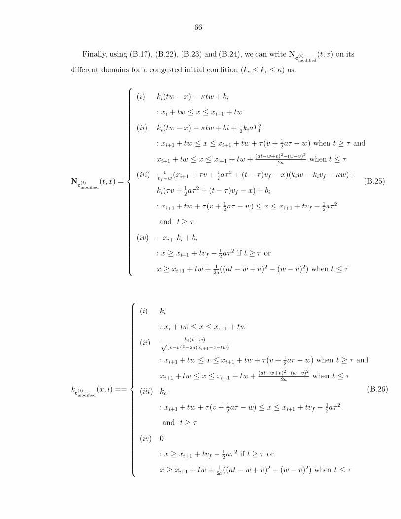
Finally, using (B.17), (B.22), (B.23) and (B.24), we can write Nc

(i)modified

(t, x) on its

different domains for a congested initial condition (kc ≤ ki ≤ κ) as:

Nc

(i)modified

(t, x) =

(i) ki(tw − x)− κtw + bi

: xi + tw ≤ x ≤ xi+1 + tw

(ii) ki(tw − x)− κtw + bi+ 12kiaT

24



2awhen t ≤ τ

(iii) 1vf−w


ki(τv + 12aτ 2 + (t− τ)vf − x) + bi


2aτ 2

and t ≥ τ

(iv) −xi+1ki + bi

: x ≥ xi+1 + tvf − 12aτ 2 if t ≥ τ or

x ≥ xi+1 + tw + 12a

((at− w + v)2 − (w − v)2) when t ≤ τ

(B.25)

kc

(i)modified

(x, t) ==

(i) ki

: xi + tw ≤ x ≤ xi+1 + tw

(ii) ki(v−w)√(v−w)2−2a(xi+1−x+tw)



2awhen t ≤ τ

(iii) kc


2aτ 2

and t ≥ τ

(iv) 0

: x ≥ xi+1 + tvf − 12aτ 2 if t ≥ τ or

x ≥ xi+1 + tw + 12a

((at− w + v)2 − (w − v)2) when t ≤ τ

(B.26)

67

C Papers Submitted and Under

Preparation

• Shanwen Qiu, Mohannad Abdelaziz, Fadl Abdellatif,and Christian G. Claudel “An

exact and grid-free numerical scheme for the hybrid two phase traffic flow model based

on the Lighthill-Whitham-Richards model with bounded acceleration”, Submitted to

Transportation Research Part B.

an exact and grid-free numerical scheme ... - kaust...

Documents