an evaluation of the system performance of a beowulf cluster - nsc
TRANSCRIPT
An evaluation of the system performance of abeowulf clusterhttp://www.nsc.liu.se/grendel/
by
Karl-Johan Andersson, Daniel Aronsson and Patrick Karlsson
Internal Report No. 2001:4
Abstract
To make accurate predictions of which type of computational problems that are suitable tosolve on a beowulf-cluster, one needs to measure the performance of the system. A beowulf-cluster can be a very good alternative too a specialized supercomputer, especially when itcomes to the price performance ratio. A beowulf-cluster is a number of commodity off-the-shelf PC’s connected through some sort of network. All basic software needed to configure acluster, and for compiling and running parallel applications on it, can be found free of chargeon the Internet.
We have configured and tested a 16-node beowulf-cluster for the Department of ScientificComputing at Uppsala University, and the National Supercomputer Centre at Linkoping,both in Sweden. We have tested both hardware and software for comparative purposes withother systems, and also for identifying characteristics of the system. Our results show that thesystem is well adopted for the type of computational jobs that the Department of ScientificComputing intend to run on the system. The tests also showed us that if the system isupgraded in the future, the course of action should be in the following order: Larger mainmemories on the nodes, faster interconnect and finally if the computational power is too low,faster processors.
Sammanfattning
For att kunna forutsaga vilka typer av berakningsproblem som framgangsrikt kan losas paett beowulf-kluster maste man mata systemets prestanda. Ett beowulf-kluster kan vara ettmycket lampligt alternativ till en superdator, sarskilt om man begrundar forhallandet mellanprestanda och pris. Ett beowulf-kluster ar ett antal vanliga persondatorer sammnkopplade iett natverk. All nodvandig mjukvara som kravs for att konfigurera klustret samt att kompileraoch kor parallella applikationer, finns fritt tillganglig pa internet.
Vi har konfigurerat och testat ett beowulf-kluster bestaende av sexton processorer atAvdelningen for teknisk databehandling vid Uppsala universitet och Nationellt Superda-torcenter vid Linkopings universitet. Vi har testat bade mjukvara och hardvara i syfte attfaststalla systemets egenskaper samt att mojliggora jamforelser med andra system. Resultat-en visar att systemet ar val lampat for att losa de typer av problem som typiskt forekommervid Avdelningen for teknisk databehandling. Testerna visar aven att eventuella framtida upp-graderingar av systemet bor ske i foljande ordning: storre minneskapacitet pa noderna, snab-bare natverk och slutligen, om storre berakningskraft behovs, snabbare processorer.
1
1 Introduction
1.1 What is a beowulf cluster?
Generally, a beowulf cluster is a set of regular PC workstations commonly interconnected throughan ethernet. It operates as a parallel computer but differs from other parallel computers in thesense that it consists of mass-produced off-the-shelf hardware. Usually, a parallell computer isbuilt of highly specialized hardware and the architecture is choosen depending on the needs. Thismakes it optimal for solving certain problems. However, it also makes it very expensive and since itoften is more or less custom built, technical support is exclusive. By constructing a beowulf clusterthese issues are solved. The penalty of going with a beowulf cluster is in reduced communicationcapacity between the processors, since an ethernet is much slower than a custom-built interconnecthardwired to a motherboard.
Recent years have shown an immense increase in the use of beowulf clusters. This is due tomainly two reasons; Firstly, the magnitude of the PC market has allowed PC prices to decreasewhile sustaining dramatic performance increase. Secondly, the linux community has produced avast asset of free software for these kinds of applications. Beowulf clusters emphasize [RBM97]
• no custom components
• dedicated processors
• a private system area network
• a freely available software base.
The name ’Beowulf’ originates from Englands oldest known epic, dating back to about 1000A.D. It tells the story of hero warrior Beowulf and his battle with the monster Grendel. Grendelis also the name of the beowulf cluster at the Department of Scientific Computing, and Beowulfwas the name of the very first beowulf cluster at NASA. In this article, we will present somemeasurements performed on Grendel, along with an implementation of a typical application atthe Department of Scientific Computing.
1.2 A brief history
The history of Beowulf cluster computers began in 1994, when Thomas Sterling and Donald Beckerat The Center of Excellence in Space Data and Information Sciences (CESDIS) were missioned toinvestigate whether clustered PCs could perform heavy computational tasks at a greater capabilitythan contemporary workstations, but at the same cost. CESDIS, which is sponsored by the NASAHPCC Earth and Space Sciences project, is often faced with tasks involving large data sets. Thefirst PC cluster, named Beowulf, was built to address problems associated with these large datasets. It consisted of 16 DX4 processors connected by a 10Mbps ethernet. Since the communicationperformance was too low to match the computational performance, Becker rewrote the ethernetdrivers and built a “channel bonded” ethernet where the network traffic was striped across two ormore ethernets [BEO].
Beowulf was an instant success. The idea of using cheap and easy-to-get equipment quicklyspread into the academic and research communities. In October of 1996, a beowulf cluster exceededone gigaflops sustained performance on a space science application for a total system cost of under$50000 [RBM97]. The cluster that this article concerns has a peak performance of just over 11gigaflops for a cost of about $15000.
1.3 System specifications
Grendel is a beowulf cluster, build from 17 separate standard PC-computers. Every computerconsists of commodity off-the-shelf products. These computers are connected together with a fastethernet network. The head of the cluster, the front-end is a separate computer that is connected
2
to the cluster and to the Internet. All jobs are submitted through this computer which takes careof scheduling and monitoring. This computer also hosts a shared file area used by the other PCs,so called nodes.
The other 16 nodes all have exactly the same configuration, both hardware and software. Thenodes have their own hard drives. Each node runs its own operating system, and accesses acommon file area through the front-end. The only difference in hardware between the front-endand the nodes is that the front-end has a second network interface card (NIC) and a slightly largerhard drive (60 GB).
All of the installed software is free and public except for the compilers (fortran and C/C++).The operating system used for all computers is RedHat Linux.
The individual computers were assembled by Advanced Computer Technology AB in Linkoping.The cluster was then put together 26-27 march 2001 at the Department of Scientific Computing,Uppsala University by system technicians from National Supercomputer Center, Linkoping Uni-versity with assistance from us.
1.3.1 Data
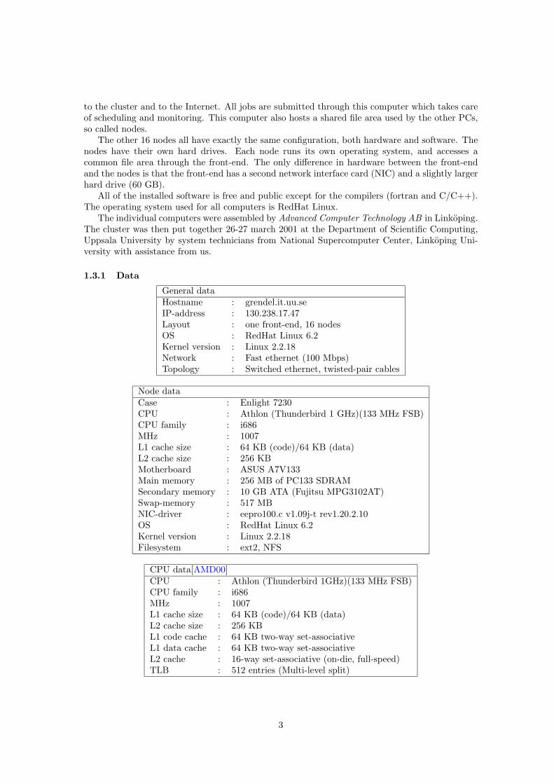
General dataHostname : grendel.it.uu.seIP-address : 130.238.17.47Layout : one front-end, 16 nodesOS : RedHat Linux 6.2Kernel version : Linux 2.2.18Network : Fast ethernet (100 Mbps)Topology : Switched ethernet, twisted-pair cables
Node dataCase : Enlight 7230CPU : Athlon (Thunderbird 1 GHz)(133 MHz FSB)CPU family : i686MHz : 1007L1 cache size : 64 KB (code)/64 KB (data)L2 cache size : 256 KBMotherboard : ASUS A7V133Main memory : 256 MB of PC133 SDRAMSecondary memory : 10 GB ATA (Fujitsu MPG3102AT)Swap-memory : 517 MBNIC-driver : eepro100.c v1.09j-t rev1.20.2.10OS : RedHat Linux 6.2Kernel version : Linux 2.2.18Filesystem : ext2, NFS
CPU data[AMD00]CPU : Athlon (Thunderbird 1GHz)(133 MHz FSB)CPU family : i686MHz : 1007L1 cache size : 64 KB (code)/64 KB (data)L2 cache size : 256 KBL1 code cache : 64 KB two-way set-associativeL1 data cache : 64 KB two-way set-associativeL2 cache : 16-way set-associative (on-die, full-speed)TLB : 512 entries (Multi-level split)
3
NetworkType : Fast ethernet (100 Mbps)Topology : Switched ethernet, single switchInterconnect : Twisted-pair (RJ45)Network switch : HP ProCurve 2424MNIC : Intel PCI EtherExpress Pro/100+ i82557NIC-driver : eepro100.c v1.09j-t rev1.20.2.10Local IP-subnet : 192.168.1.0/255.255.255.0
2 Installed software
2.1 Operating system
The operating system installed is Linux. The distribution used is RedHat 6.2 with additionalupdates. The currently running Linux kernel is version 2.2.18. The kernel is recompiled to matchour needs. There are also some extra kernel modules compiled for hardware monitoring.
2.2 Programming environment
The programming languages intended for use are Fortran and C.As parallel processing has matured, two programming paradigms have been developed, shared
memory and message passing. These paradigms have their origin in different hardware architec-tures. Shared memory-programming is mainly intended for high-end-computers which actuallyhave a shared memory. Each processor has access to all memory, or some partition thereof. Mes-sage passing on the other hand originates from distributed memory machines. Here every processorhas its own memory-area and communicates with the others by sending messages.
Not surprisingly message passing has become the most popular technique for implementingparallel applications on beowulf clusters. Currently there are no shared memory-libraries installedon Grendel. The most well known APIs that use the message passing paradigm in parallel com-putations are MPI and PVM. Both of these are installed on Grendel by NSC but PVM is nottested since it is not used at the Department of Scientific Computing.
There are two different sets of compilers installed; EGCS 2.91.66 that is installed with theRedHat Linux-distribution, and the Portland Group Workstation compilers (PG 3.2-3).
EGCSC : gcc, cc /usr/bin/gccC++ : g++ /usr/bin/g++Fortran-77 : f77 /usr/bin/f77Portland GroupC : pgcc /usr/local/pgi/linux86/bin/pgccC++ : pgCC /usr/local/pgi/linux86/bin/pgCCFortran-77 : pgf77 /usr/local/pgi/linux86/bin/pgf77Fortran-90 : pgf90 /usr/local/pgi/linux86/bin/pgf90HPF : pghpf /usr/local/pgi/linux86/bin/pghpf
The recommended compilers to use for high-performance-applications are the Portland Groupcompilers. These are commercial products intended for high-performance computing.
2.3 MPI libraries
The Message Passing Interface (MPI) is a standard for writing applications using the message-passing paradigm. This standard is supervised by the MPI Forum, which is comprised of highperformance computing professionals from over 40 organizations [MPI95]. The goal of MPI Forumis to form a standard for message-passing applications which meets the needs of the majority of
4
users. MPI provides a framework for vendors to implement efficient implementations. This ensuresthat program written for MPI compiles for all implementations, but efficiency may differ.
The two by far most popular choices for clusters are MPICH and LAM/MPI. Both these arefree implementations of the MPI standard. Both cover MPI version 1.1 completely (MPICH fullyimplements 1.2) and part of version 2.0.
The MPI Chameleon (MPICH) was developed at Argonne National Laboratory as a researchproject to provide features that would make MPI implementation simple on different architectures.To do this MPICH implements a middle-layer called Abstract Device Interface (ADI). This hasa smaller interface making it easier to implement on different hardware, but it also may decreaseefficiency.
Local Area Multicomputer (LAM) was originally developed at the Ohio Super ComputingFacility but is now maintained by the Laboratory of Scientific Computing at Notre Dame. LAMis built to be more ”cluster friendly” by using small daemons to effect achieve fast process control.MPICH on the other hand uses system daemons to control processes.
As we will see (see 4.2.2) LAM seems to be the best choice for writing parallel applications forthis cluster. All further tests and benchmarks in this report use LAM for message-passing.
Both these implementations use TCP/IP as the underlying protocol and are thus limited bythis.
Both these implementations are installed on Grendel and are avaliable for use.LAM and MPICH use two different strategies for running parallel programs. Both of them are
run through the command mpirun which spawns the processes to the different processors. LAMuses a user level daemon that controls communication between different processors. For this towork one first needs to start up this program through the command lamboot on each node. Inour case there is also a scheduler that schedules the right number of processors to the application.The daemon runs in user-mode so there is a need to run this program for each user that submitsjobs to the cluster. LAM also implements the MPI 2.0 MPI Spawn call that allows tasks to bespawned from within the application, as opposed to running a program like mpirun.
NSC in Linkoping has created a version of mpirun which first runs lamboot and then calls thereal mpirun. After finishing it calls lamhalt on each node to clean up. So there are never twoinstances of the daemon running on any node at the same time, assuring that an application haveexclusive use of the requested processors.
MPICH on the other hand attempts to start remote processes by connecting to a default systemlevel daemon, or by using remote shell. This means that you don’t have to run a specific daemonfor each user.
Both LAM and MPICH use TCP/IP as the underlying communications layer. LAM commu-nicates using mainly UDP-packets. It can be configured to use TCP-connections instead (usingthe c2c-option for lamboot). All necessary connections are established between the daemons atstartup by lamboot and are closed when calling lamhalt.
We have not done any test on TCP versus UDP-traffic but according to [CLMR00] UDP issuperior to TCP in the case of MPI. We have done some raw benchmark tests for TCP (see3.2.2 and 3.4.1) but no comparing tests for TCP versus UDP using MPI. Since this network is adedicated local area network, in fact every node is connected to a single full-duplex switch, thereis no need for flow control and congestion control supported by TCP. TCP has some drawbacksfor this type of traffic. This includes the slow start feature that checks the congestion levelin the communication network. According to [CLMR00] this feature slows down performanceconsiderably. By modifying the TCP-options in the Linux kernel this can be turned off.
Applications pass messages through standard UNIX stream sockets to the LAM-daemon, whichthen communicates with the other daemons on the other nodes (using UDP, see above). Thedaemon on the remote machine then passes the message to the application through a UNIXstream socket.
5
2.3.1 Latencies in MPI
We want to establish a simple model for latency for the different steps in the communicationprocedure using MPI. How much overhead does MPI introduce and which message size is optimal?To find out this we use a simple ping-pong program that sends a message between two nodes andmeasures network traffic. See appendix D for source code.
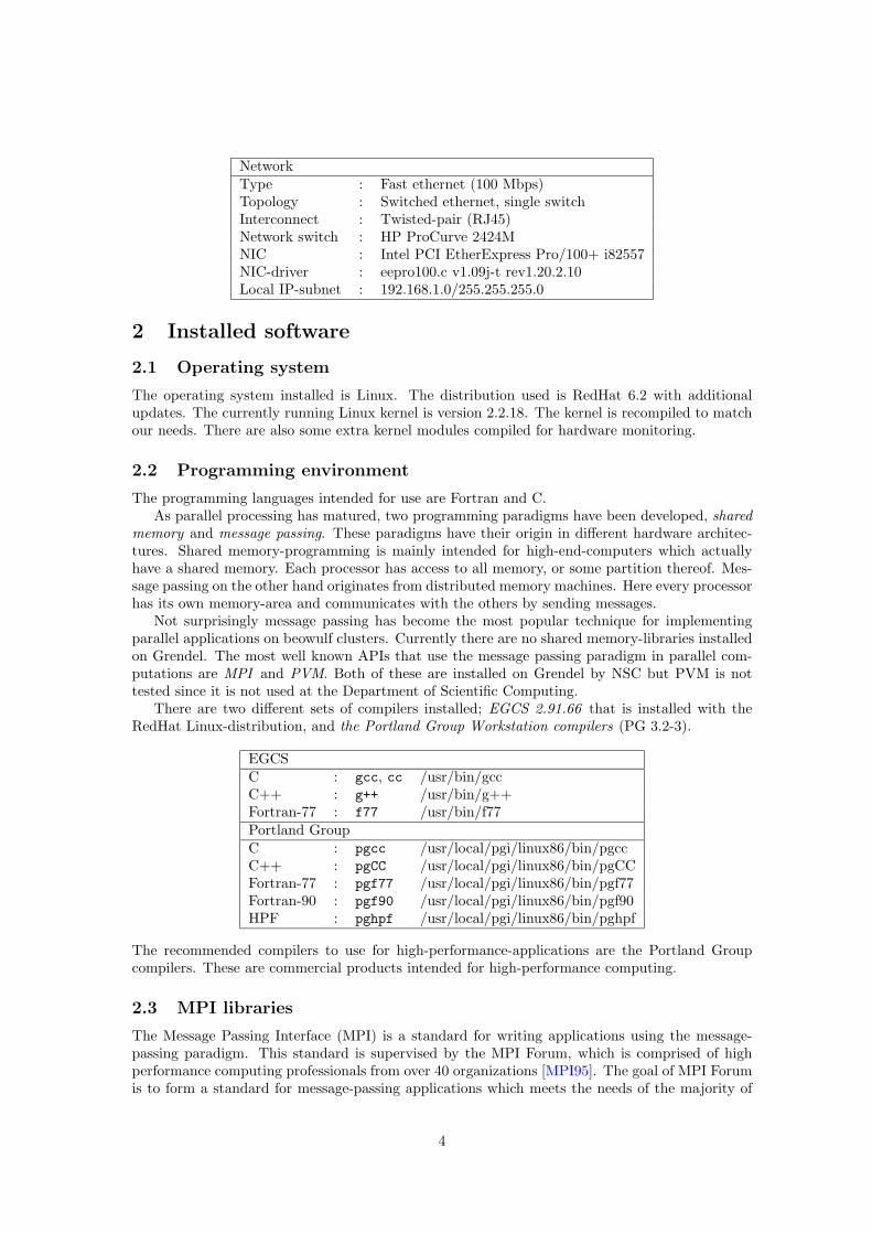
The program sends messages of different sizes and measures the average time to send andreceive the message, number of bytes and packets sent and received. The information of thenumber of bytes and packets was gathered from the Linux kernel and shows the actual number ofbytes sent and received from a specific network interface card. This includs IP and UDP headersand additional MPI overhead. The number of packets is the total number of ethernet frames sentand received. So if a single packet is fragmented into several frames it is the resulting frames thatare counted, not the original number of packets.
0 500 1000 1500 2000 2500 3000 3500 40000
500
1000
1500
Message size in bytes
Byt
es p
er p
acke
t
Figure 1: Bytes per packet for different message sizes
Figure 1 shows the number of bytes per packet for different message sizes in MPI. We can clearlysee the MTU limit (Maximum Transfer Unit) at 1500 bytes introduced by IP. When packets reachthe 1500-bytes limit they are split up into two packets. We can see in the graph that when wesend a MPI-message of 1600 bytes it results in two IP-packets of 850 bytes each, a total overheadof 100 bytes (including UPD- and IP-headers). Below 1500 bytes there is an overhead of 89 bytes.This shows that the MPI daemon is unaware of the underlying network limits.
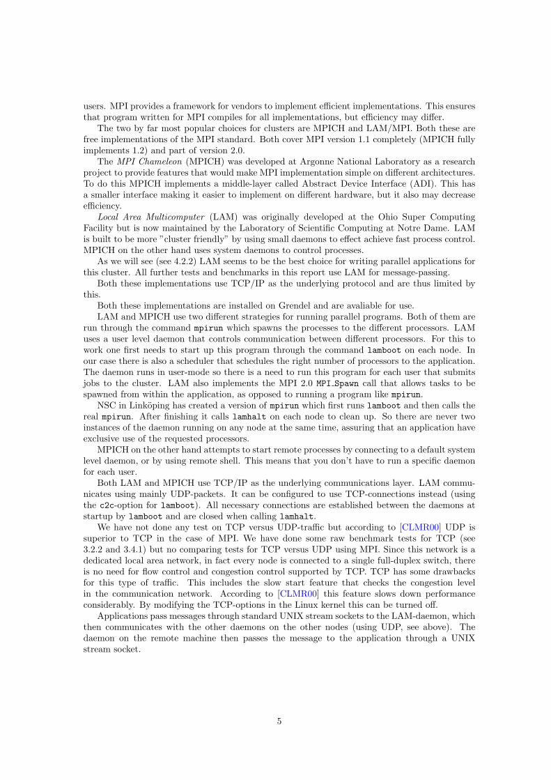
However it seems that this is not a substantial drawback for the communication performance.Figure 2 show the number of packets transmitted per second over the same interval. The lower thepacket size the more packets can be transmitted per second. Thus the total bandwidth increaseswith larger messages. The effect of packet limitations seems not to be that limiting on bandwidth.
Timings from this program give an RTT (Round Trip Time) of 130 µs for sending and receivingone empty packet. This results in approximately 65 µs latency for one MPI-message.
To do further timing, and to get better results, we used the benchmark program netpipe fromScalable Computing Lab [SMG96]. This program is similar to pingpong but could be set up to runon different systems, like pure TCP/IP, MPI and PVM. We tested this program on pure IP-trafficand MPI (using LAM). Netpipe was compiled using pgcc with no additional compiler flags. It wasrun by using the command
NPtcp -t -h node -o output.txt -P
6
0 500 1000 1500 2000 2500 3000 3500 40000
1000
2000
3000
4000
5000
6000
7000
8000
Message size in bytes
Pac
kets
per
sec
ond
Figure 2: Packets per second for different message sizes
mpirun -np 2 NPmpi -o output.txt -P
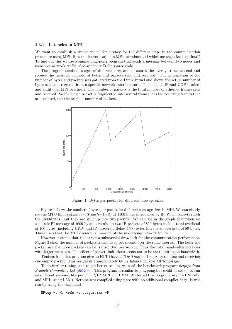
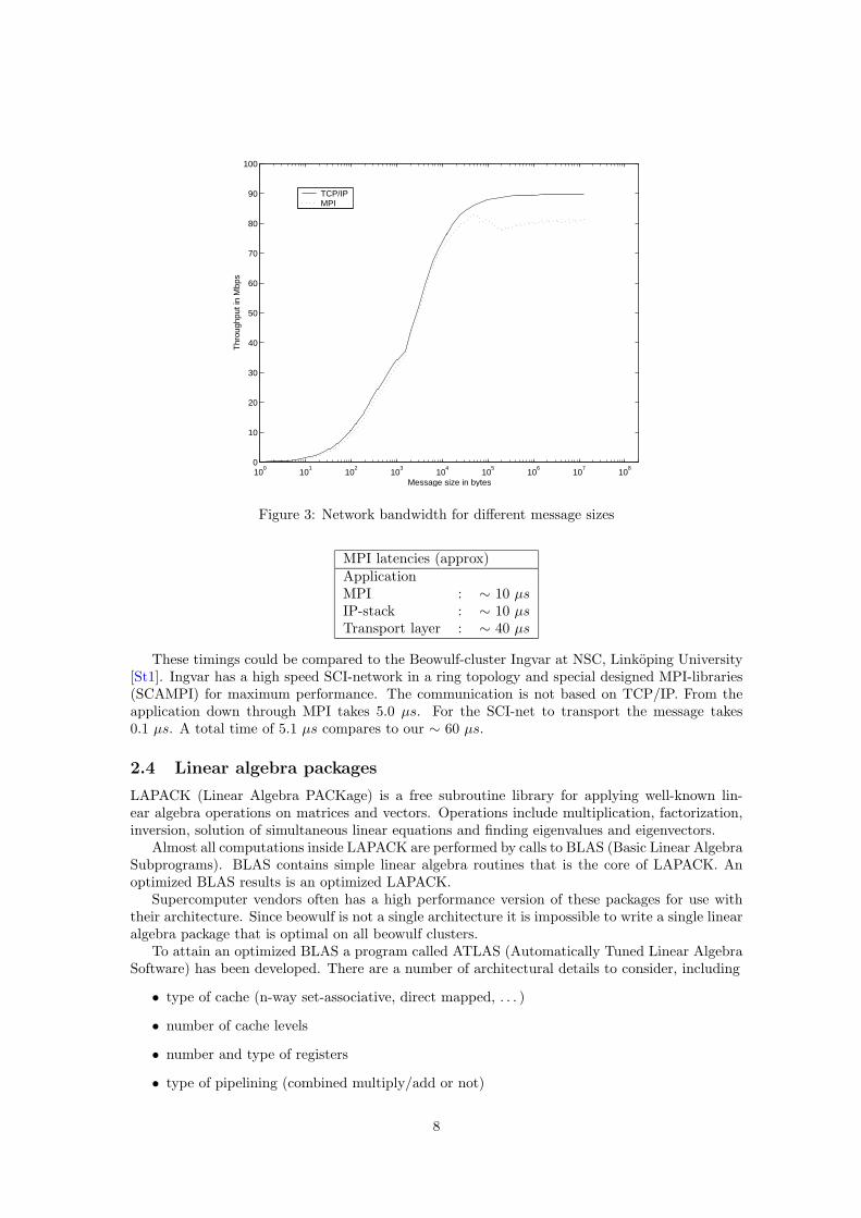
Figure 3 shows a signature graph for TCP/IP and MPI-communication, i e bandwidth againstmessage size. The theoretical maximum bandwidth for fast ethernet is 100 Mbps. As we can see,bandwidth for TCP/IP is increasing up to 90 Mbps and then stays there (at least for messagesup to 20 MB). MPI follows that curve up until 80 kB when it suddenly drops down to about80 Mbps. This is probably because LAM changes communication strategy. From this it is possibleto calculate latencies for sending empty packets for both IP and MPI. We got 52 µs for IP and62 µs for MPI traffic. The variance in these measurement was below 1% according to netpipe.
To test the congestion level in the switch we set up this test program at eight nodes at thesame time, each node sending and receiving 90 Mbps. There was no noticeable decrease in networkperformance.
To find out which part of the time is due to actual communications and which is due toTCP/IP-implementation we ran the same program locally on one computer. You can force LAMto run two processes on the same processor by giving the -np 2 option to mpirun but only makeone node avaliable through lamboot. To time local TCP/IP traffic you just run both the serverand client on the same computer.
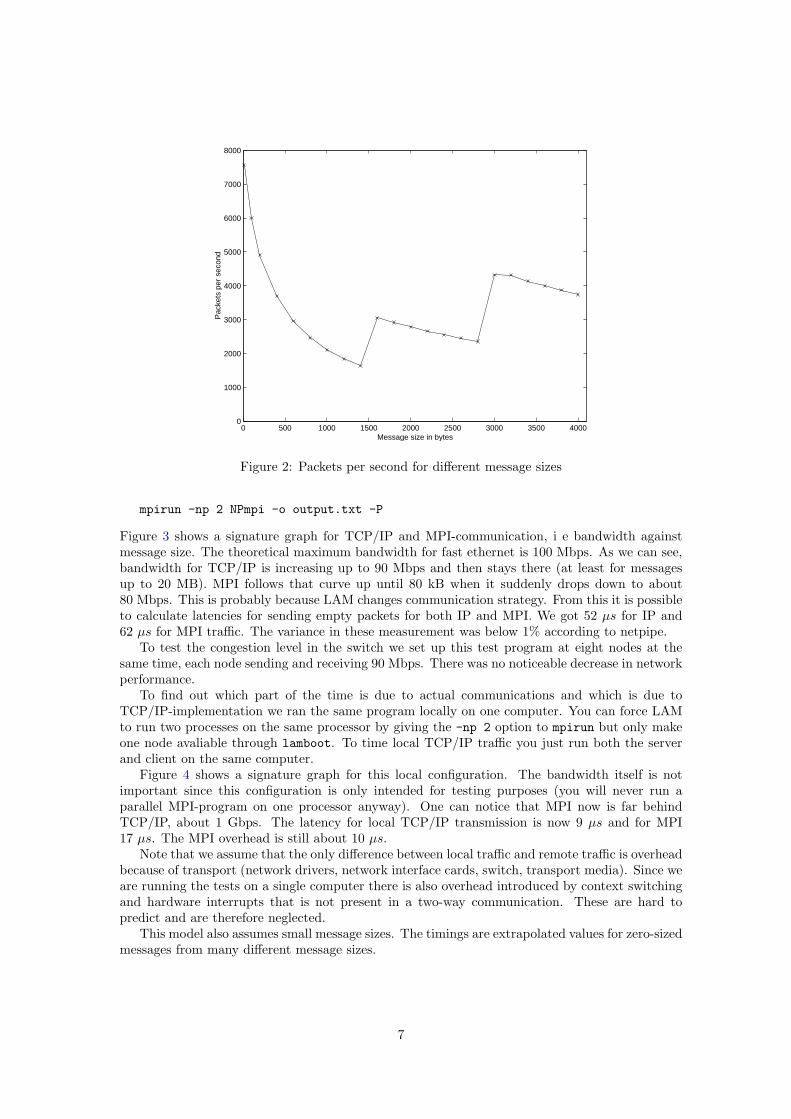
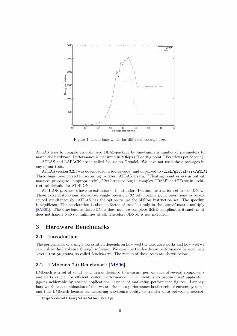
Figure 4 shows a signature graph for this local configuration. The bandwidth itself is notimportant since this configuration is only intended for testing purposes (you will never run aparallel MPI-program on one processor anyway). One can notice that MPI now is far behindTCP/IP, about 1 Gbps. The latency for local TCP/IP transmission is now 9 µs and for MPI17 µs. The MPI overhead is still about 10 µs.
Note that we assume that the only difference between local traffic and remote traffic is overheadbecause of transport (network drivers, network interface cards, switch, transport media). Since weare running the tests on a single computer there is also overhead introduced by context switchingand hardware interrupts that is not present in a two-way communication. These are hard topredict and are therefore neglected.
This model also assumes small message sizes. The timings are extrapolated values for zero-sizedmessages from many different message sizes.
7
100
101
102
103
104
105
106
107
108
0
10
20
30
40
50
60
70
80
90
100
Message size in bytes
Thr
ough
put i
n M
bps
TCP/IPMPI
Figure 3: Network bandwidth for different message sizes
MPI latencies (approx)ApplicationMPI : ∼ 10 µsIP-stack : ∼ 10 µsTransport layer : ∼ 40 µs
These timings could be compared to the Beowulf-cluster Ingvar at NSC, Linkoping University[St1]. Ingvar has a high speed SCI-network in a ring topology and special designed MPI-libraries(SCAMPI) for maximum performance. The communication is not based on TCP/IP. From theapplication down through MPI takes 5.0 µs. For the SCI-net to transport the message takes0.1 µs. A total time of 5.1 µs compares to our ∼ 60 µs.
2.4 Linear algebra packages
LAPACK (Linear Algebra PACKage) is a free subroutine library for applying well-known lin-ear algebra operations on matrices and vectors. Operations include multiplication, factorization,inversion, solution of simultaneous linear equations and finding eigenvalues and eigenvectors.
Almost all computations inside LAPACK are performed by calls to BLAS (Basic Linear AlgebraSubprograms). BLAS contains simple linear algebra routines that is the core of LAPACK. Anoptimized BLAS results is an optimized LAPACK.
Supercomputer vendors often has a high performance version of these packages for use withtheir architecture. Since beowulf is not a single architecture it is impossible to write a single linearalgebra package that is optimal on all beowulf clusters.
To attain an optimized BLAS a program called ATLAS (Automatically Tuned Linear AlgebraSoftware) has been developed. There are a number of architectural details to consider, including
• type of cache (n-way set-associative, direct mapped, . . . )
• number of cache levels
• number and type of registers
• type of pipelining (combined multiply/add or not)
8
100
101
102
103
104
105
106
107
108
0
500
1000
1500
2000
2500
3000
Message size in bytes
Thr
ough
put i
n M
bps
TCP/IPMPI
Figure 4: Local bandwidth for different message sizes
ATLAS tries to compile an optimized BLAS-package by fine-tuning a number of parameters tomatch the hardware. Performance is measured in Mflops (FLoating point OPerations per Second).
ATLAS and LAPACK are installed for use on Grendel. We have not used these packages inany of our tests.
ATLAS version 3.2.1 was downloaded in source code1 and unpacked to /disk/global/src/ATLAS.Three bugs were corrected according to latest ATLAS errata: ”Floating point errors in outputmatrices propagate inappropriately”, ”Performance bug in complex TRSM” and ”Error in archi-tectural defaults for ATHLON”.
ATHLON processors have an extension of the standard Pentium instruction set called 3DNow.These extra instructions allows two single precision (32 bit) floating point operations to be ex-ecuted simultaneously. ATLAS has the option to use the 3DNow instruction set. The speedupis significant; The acceleration is about a factor of two, but only in the case of matrix-multiply[SAR01]. The drawback is that 3DNow does not use complete IEEE compliant arithmetics. Itdoes not handle NaNs or Infinities at all. Therefore 3DNow is not included.
3 Hardware Benchmarks
3.1 Introduction
The performance of a single workstation depends on how well the hardware works and how well wecan utilize the hardware through software. We examine the hardware performance by executingseveral test programs, so called benchmarks. The results of these tests are shown below.
3.2 LMbench 2.0 Benchmark [MS96]
LMbench is a set of small benchmarks designed to measure performance of several componentsand parts crucial for efficient system performance. The intent is to produce real applicationfigures achievable by normal applications, instead of marketing performance figures. Latency,bandwidth or a combination of the two are the main performance bottlenecks of current systems,and thus LMbench focuses on measuring a system’s ability to transfer data between processor,
1http://www.netlib.org/atlas/atlas3.2.1.tgz
9
cache, memory, network and disk. It does not measure graphics throughput, computational speedor any multiprocessor features.
3.2.1 Implementation
LMbench is highly portable and should run as is with gcc as default compiler. For the cluster thatwould be the GNU project C compiler (egcs-1.1.2). The basic system parameters are describedbelow.
Basic system parametersHost : grendel.it.uu.seCPU : Athlon (Thunderbird)(133 MHz FSB) (×17)CPU family : i686MHz : 1007L1 cache size : 64 KB (code)/64 KB (data)L2 cache size : 256 KBMotherboard : ASUS A7V133Main memory : 256 MB of PC133 SDRAMSecondary memory : 10 GB ATAOS kernel : Linux 2.2.18Network : Intel 100/PRO+ NICNetwork switch : HP ProCurve 2424M
The benchmark tests six different aspects of the system:
• Processor and processes
• Context switching
• Communication latencies
• File and virtual memory system latencies
• Communication bandwidths
• Memory latencies
3.2.2 Results
The results are an average of ten independent runs of LMbench 2.0 to ensure accuracy. We alsoinclude an error estimate in the result, based on one standard deviation.
Processor, processes (µs) - smaller is betternull call : 0.27 ± 0.000null I/O : 0.38 ± 0.035stat : 3.72 ± 0.167open/close : 4.63 ± 0.149select : 26.3 ± 10.56signal install : 0.77 ± 0.003signal catch : 0.95 ± 0.000fork proc : 110.1 ± 2.47exec proc : 706.2 ± 25.93shell proc : 3605.3 ± 35.99
Null system call The time it takes to do getppid. This is useful as a lower bound cost onanything that has to interact with the operating system.
null I/O The time it takes to write one byte to /dev/null.
10
stat Measures how long it takes to stat a file (i e examine a files characteristics.).
open/close The time it takes to first open a file and then close it.
Simple entry into the operating system The time it takes to run select on a number of filedescriptors.
Signal handling latencies The time it takes to install or catch signals.
Creates a process through fork+exit The purpose of the three last benchmarks is to timethe creation of a basic thread of control. It measures the time it takes to split a process intotwo copies, but it is not very useful since the processes perform the same thing.
Creates a process through fork+execve The time it takes to create a new process and havethat process perform a new task.
Creates a process through fork+/bin/sh -c The time it takes to create a new process andhave the new process running a program by asking the shell to find that program and runit.
Context switching (µs) - smaller is better2p/0K : 0.870 ± 0.18032p/16K : 1.6200 ± 0.188802p/64K : 15.8 ± 0.428p/16K : 5.4410 ± 0.373538p/64K : 117.7 ± 0.4816p/16K : 15.4 ± 1.3516p/64K : 117.7 ± 0.48
Context switching The time it takes for n processes of size s (i.e. np/sK) to switch context.The processes are connected in a ring of UNIX pipes.
Local communication latencies (µs) - smaller is betterpipe : 4.021 ± 0.3027AF UNIX : 8.34 ± 0.833UDP : 11.5 ± 0.53RPC/UDP : 26.4 ± 0.84TCP : 16.4 ± 1.35RPC/TCP : 39.1 ± 0.74
Interprocess communication latency through pipes Measures the interprocess communi-cation latencies between two processes communicating through a UNIX pipe. The contextswitching overhead is included and the result is per round trip.
Interprocess communication latency through UNIX sockets Measures the time it takesto send a token back and forth between two processes using a UNIX socket.
Interprocess communication latency via UDP/IP The benchmark measures the time ittakes to pass a token back and forth between a client/server. No work is done in theprocesses.
Interprocess communication latency through SUN RPC via UDP The time it takes toperform the benchmark above using SUN RPC instead of standard UDP sockets.
Interprocess communication latency via TCP/IP The benchmark measures the time it takesto pass a token back and forth between a client/server. No work is done in the processes.
Interprocess communication latency through SUN RPC via TCP The time it takes toperform the benchmark above using SUN RPC instead of standard UDP sockets.
11
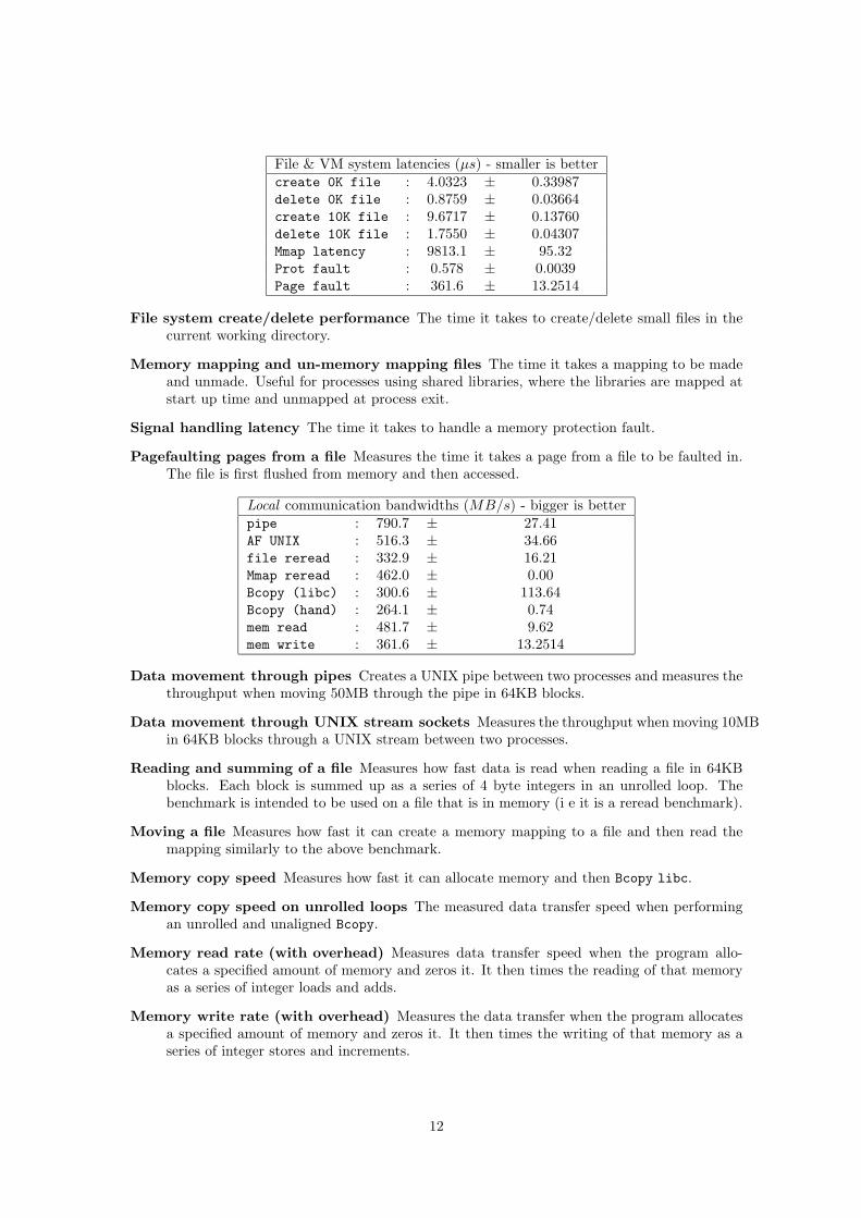
File & VM system latencies (µs) - smaller is bettercreate 0K file : 4.0323 ± 0.33987delete 0K file : 0.8759 ± 0.03664create 10K file : 9.6717 ± 0.13760delete 10K file : 1.7550 ± 0.04307Mmap latency : 9813.1 ± 95.32Prot fault : 0.578 ± 0.0039Page fault : 361.6 ± 13.2514
File system create/delete performance The time it takes to create/delete small files in thecurrent working directory.
Memory mapping and un-memory mapping files The time it takes a mapping to be madeand unmade. Useful for processes using shared libraries, where the libraries are mapped atstart up time and unmapped at process exit.
Signal handling latency The time it takes to handle a memory protection fault.
Pagefaulting pages from a file Measures the time it takes a page from a file to be faulted in.The file is first flushed from memory and then accessed.
Local communication bandwidths (MB/s) - bigger is betterpipe : 790.7 ± 27.41AF UNIX : 516.3 ± 34.66file reread : 332.9 ± 16.21Mmap reread : 462.0 ± 0.00Bcopy (libc) : 300.6 ± 113.64Bcopy (hand) : 264.1 ± 0.74mem read : 481.7 ± 9.62mem write : 361.6 ± 13.2514
Data movement through pipes Creates a UNIX pipe between two processes and measures thethroughput when moving 50MB through the pipe in 64KB blocks.
Data movement through UNIX stream sockets Measures the throughput when moving 10MBin 64KB blocks through a UNIX stream between two processes.
Reading and summing of a file Measures how fast data is read when reading a file in 64KBblocks. Each block is summed up as a series of 4 byte integers in an unrolled loop. Thebenchmark is intended to be used on a file that is in memory (i e it is a reread benchmark).
Moving a file Measures how fast it can create a memory mapping to a file and then read themapping similarly to the above benchmark.
Memory copy speed Measures how fast it can allocate memory and then Bcopy libc.
Memory copy speed on unrolled loops The measured data transfer speed when performingan unrolled and unaligned Bcopy.
Memory read rate (with overhead) Measures data transfer speed when the program allo-cates a specified amount of memory and zeros it. It then times the reading of that memoryas a series of integer loads and adds.
Memory write rate (with overhead) Measures the data transfer when the program allocatesa specified amount of memory and zeros it. It then times the writing of that memory as aseries of integer stores and increments.
12
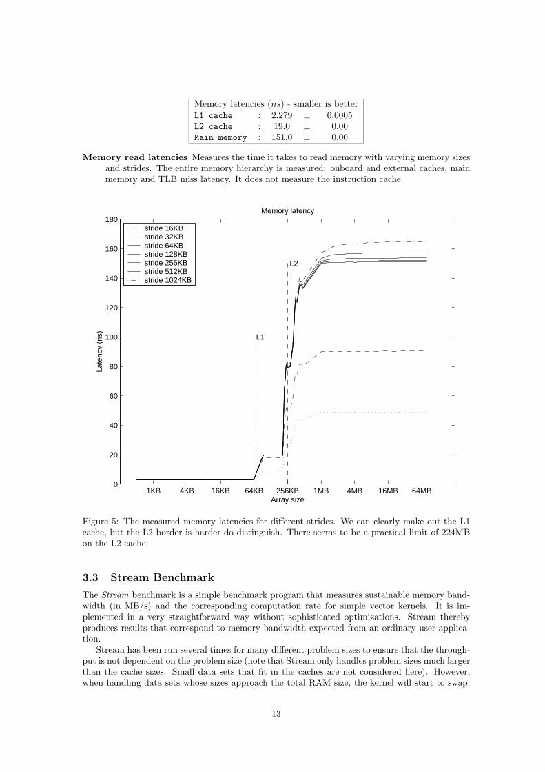
Memory latencies (ns) - smaller is betterL1 cache : 2.279 ± 0.0005L2 cache : 19.0 ± 0.00Main memory : 151.0 ± 0.00
Memory read latencies Measures the time it takes to read memory with varying memory sizesand strides. The entire memory hierarchy is measured: onboard and external caches, mainmemory and TLB miss latency. It does not measure the instruction cache.
1KB 4KB 16KB 64KB 256KB 1MB 4MB 16MB 64MB0
20
40
60
80
100
120
140
160
180
L1
L2
Memory latency
Late
ncy
(ns)
Array size
stride 16KB stride 32KB stride 64KB stride 128KB stride 256KB stride 512KB stride 1024KB
Figure 5: The measured memory latencies for different strides. We can clearly make out the L1cache, but the L2 border is harder do distinguish. There seems to be a practical limit of 224MBon the L2 cache.
3.3 Stream Benchmark
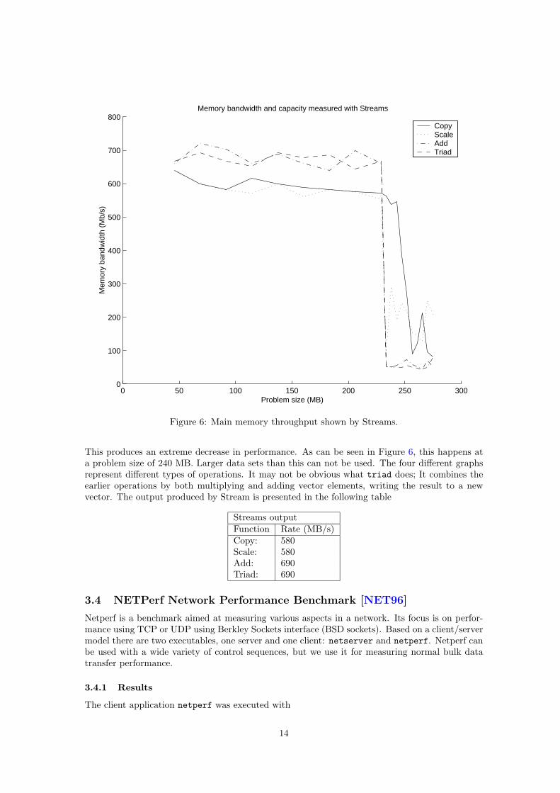
The Stream benchmark is a simple benchmark program that measures sustainable memory band-width (in MB/s) and the corresponding computation rate for simple vector kernels. It is im-plemented in a very straightforward way without sophisticated optimizations. Stream therebyproduces results that correspond to memory bandwidth expected from an ordinary user applica-tion.
Stream has been run several times for many different problem sizes to ensure that the through-put is not dependent on the problem size (note that Stream only handles problem sizes much largerthan the cache sizes. Small data sets that fit in the caches are not considered here). However,when handling data sets whose sizes approach the total RAM size, the kernel will start to swap.
13
0 50 100 150 200 250 3000
100
200
300
400
500
600
700
800Memory bandwidth and capacity measured with Streams
Problem size (MB)
Mem
ory
band
wid
th (
Mb/
s)
CopyScaleAddTriad
Figure 6: Main memory throughput shown by Streams.
This produces an extreme decrease in performance. As can be seen in Figure 6, this happens ata problem size of 240 MB. Larger data sets than this can not be used. The four different graphsrepresent different types of operations. It may not be obvious what triad does; It combines theearlier operations by both multiplying and adding vector elements, writing the result to a newvector. The output produced by Stream is presented in the following table
Streams outputFunction Rate (MB/s)Copy: 580Scale: 580Add: 690Triad: 690
3.4 NETPerf Network Performance Benchmark [NET96]
Netperf is a benchmark aimed at measuring various aspects in a network. Its focus is on perfor-mance using TCP or UDP using Berkley Sockets interface (BSD sockets). Based on a client/servermodel there are two executables, one server and one client: netserver and netperf. Netperf canbe used with a wide variety of control sequences, but we use it for measuring normal bulk datatransfer performance.
3.4.1 Results
The client application netperf was executed with
14
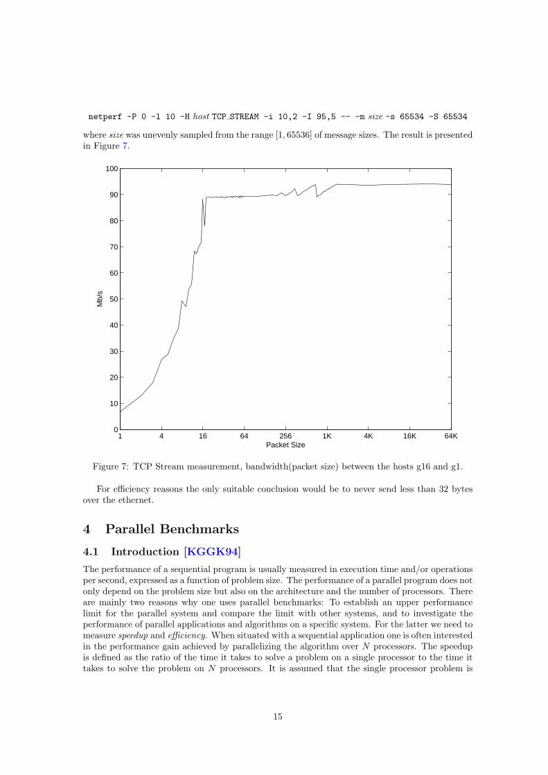
netperf -P 0 -l 10 -H host TCP STREAM -i 10,2 -I 95,5 -- -m size -s 65534 -S 65534
where size was unevenly sampled from the range [1, 65536] of message sizes. The result is presentedin Figure 7.
1 4 16 64 256 1K 4K 16K 64K0
10
20
30
40
50
60
70
80
90
100
Packet Size
Mb/
s
Figure 7: TCP Stream measurement, bandwidth(packet size) between the hosts g16 and g1.
For efficiency reasons the only suitable conclusion would be to never send less than 32 bytesover the ethernet.
4 Parallel Benchmarks
4.1 Introduction [KGGK94]
The performance of a sequential program is usually measured in execution time and/or operationsper second, expressed as a function of problem size. The performance of a parallel program does notonly depend on the problem size but also on the architecture and the number of processors. Thereare mainly two reasons why one uses parallel benchmarks: To establish an upper performancelimit for the parallel system and compare the limit with other systems, and to investigate theperformance of parallel applications and algorithms on a specific system. For the latter we need tomeasure speedup and efficiency. When situated with a sequential application one is often interestedin the performance gain achieved by parallelizing the algorithm over N processors. The speedupis defined as the ratio of the time it takes to solve a problem on a single processor to the time ittakes to solve the problem on N processors. It is assumed that the single processor problem is
15
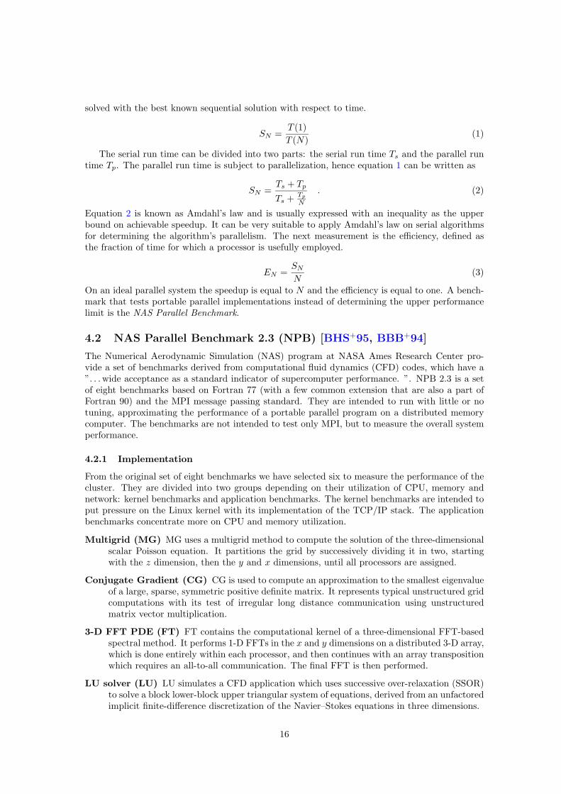
solved with the best known sequential solution with respect to time.
SN =T (1)T (N)
(1)
The serial run time can be divided into two parts: the serial run time Ts and the parallel runtime Tp. The parallel run time is subject to parallelization, hence equation 1 can be written as
SN =Ts + Tp
Ts + TpN
. (2)
Equation 2 is known as Amdahl’s law and is usually expressed with an inequality as the upperbound on achievable speedup. It can be very suitable to apply Amdahl’s law on serial algorithmsfor determining the algorithm’s parallelism. The next measurement is the efficiency, defined asthe fraction of time for which a processor is usefully employed.
EN =SNN
(3)
On an ideal parallel system the speedup is equal to N and the efficiency is equal to one. A bench-mark that tests portable parallel implementations instead of determining the upper performancelimit is the NAS Parallel Benchmark.
4.2 NAS Parallel Benchmark 2.3 (NPB) [BHS+95, BBB+94]
The Numerical Aerodynamic Simulation (NAS) program at NASA Ames Research Center pro-vide a set of benchmarks derived from computational fluid dynamics (CFD) codes, which have a”. . . wide acceptance as a standard indicator of supercomputer performance. ”. NPB 2.3 is a setof eight benchmarks based on Fortran 77 (with a few common extension that are also a part ofFortran 90) and the MPI message passing standard. They are intended to run with little or notuning, approximating the performance of a portable parallel program on a distributed memorycomputer. The benchmarks are not intended to test only MPI, but to measure the overall systemperformance.
4.2.1 Implementation
From the original set of eight benchmarks we have selected six to measure the performance of thecluster. They are divided into two groups depending on their utilization of CPU, memory andnetwork: kernel benchmarks and application benchmarks. The kernel benchmarks are intended toput pressure on the Linux kernel with its implementation of the TCP/IP stack. The applicationbenchmarks concentrate more on CPU and memory utilization.
Multigrid (MG) MG uses a multigrid method to compute the solution of the three-dimensionalscalar Poisson equation. It partitions the grid by successively dividing it in two, startingwith the z dimension, then the y and x dimensions, until all processors are assigned.
Conjugate Gradient (CG) CG is used to compute an approximation to the smallest eigenvalueof a large, sparse, symmetric positive definite matrix. It represents typical unstructured gridcomputations with its test of irregular long distance communication using unstructuredmatrix vector multiplication.
3-D FFT PDE (FT) FT contains the computational kernel of a three-dimensional FFT-basedspectral method. It performs 1-D FFTs in the x and y dimensions on a distributed 3-D array,which is done entirely within each processor, and then continues with an array transpositionwhich requires an all-to-all communication. The final FFT is then performed.
LU solver (LU) LU simulates a CFD application which uses successive over-relaxation (SSOR)to solve a block lower-block upper triangular system of equations, derived from an unfactoredimplicit finite-difference discretization of the Navier–Stokes equations in three dimensions.
16
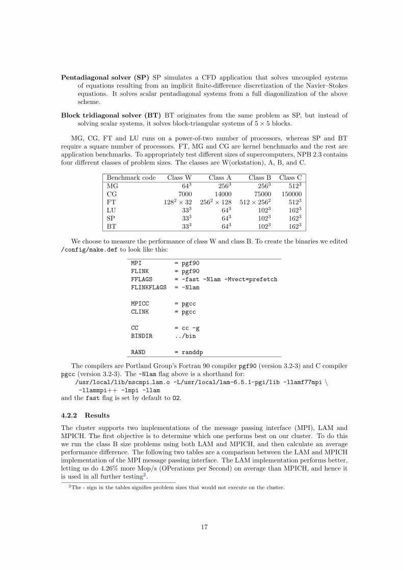
Pentadiagonal solver (SP) SP simulates a CFD application that solves uncoupled systemsof equations resulting from an implicit finite-difference discretization of the Navier–Stokesequations. It solves scalar pentadiagonal systems from a full diagonilization of the abovescheme.
Block tridiagonal solver (BT) BT originates from the same problem as SP, but instead ofsolving scalar systems, it solves block-triangular systems of 5× 5 blocks.
MG, CG, FT and LU runs on a power-of-two number of processors, whereas SP and BTrequire a square number of processors. FT, MG and CG are kernel benchmarks and the rest areapplication benchmarks. To appropriately test different sizes of supercomputers, NPB 2.3 containsfour different classes of problem sizes. The classes are W(orkstation), A, B, and C.
Benchmark code Class W Class A Class B Class CMG 643 2563 2563 5123
CG 7000 14000 75000 150000FT 1282 × 32 2562 × 128 512× 2562 5123
LU 333 643 1023 1623
SP 333 643 1023 1623
BT 333 643 1023 1623
We choose to measure the performance of class W and class B. To create the binaries we edited/config/make.def to look like this:
MPI = pgf90FLINK = pgf90FFLAGS = -fast -Nlam -Mvect=prefetchFLINKFLAGS = -Nlam
MPICC = pgccCLINK = pgcc
CC = cc -gBINDIR ../bin
RAND = randdp
The compilers are Portland Group’s Fortran 90 compiler pgf90 (version 3.2-3) and C compilerpgcc (version 3.2-3). The -Nlam flag above is a shorthand for:
/usr/local/lib/nscmpi lam.o -L/usr/local/lam-6.5.1-pgi/lib -llamf77mpi \-llammpi++ -lmpi -llam
and the fast flag is set by default to O2.
4.2.2 Results
The cluster supports two implementations of the message passing interface (MPI), LAM andMPICH. The first objective is to determine which one performs best on our cluster. To do thiswe run the class B size problems using both LAM and MPICH, and then calculate an averageperformance difference. The following two tables are a comparison between the LAM and MPICHimplementation of the MPI message passing interface. The LAM implementation performs better,letting us do 4.26% more Mop/s (OPerations per Second) on average than MPICH, and hence itis used in all further testing2.
2The - sign in the tables signifies problem sizes that would not execute on the cluster.
17
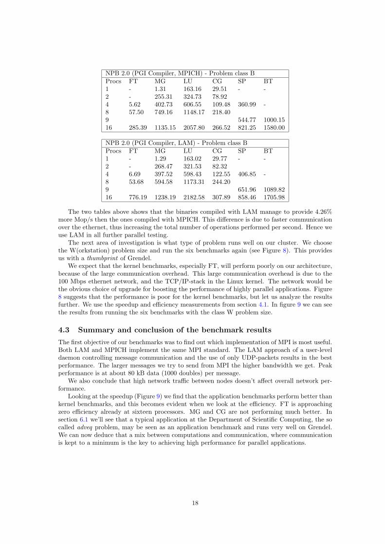
NPB 2.0 (PGI Compiler, MPICH) - Problem class BProcs FT MG LU CG SP BT1 - 1.31 163.16 29.51 - -2 - 255.31 324.73 78.924 5.62 402.73 606.55 109.48 360.99 -8 57.50 749.16 1148.17 218.409 544.77 1000.1516 285.39 1135.15 2057.80 266.52 821.25 1580.00
NPB 2.0 (PGI Compiler, LAM) - Problem class BProcs FT MG LU CG SP BT1 - 1.29 163.02 29.77 - -2 - 268.47 321.53 82.324 6.69 397.52 598.43 122.55 406.85 -8 53.68 594.58 1173.31 244.209 651.96 1089.8216 776.19 1238.19 2182.58 307.89 858.46 1705.98
The two tables above shows that the binaries compiled with LAM manage to provide 4.26%more Mop/s then the ones compiled with MPICH. This difference is due to faster communicationover the ethernet, thus increasing the total number of operations performed per second. Hence weuse LAM in all further parallel testing.
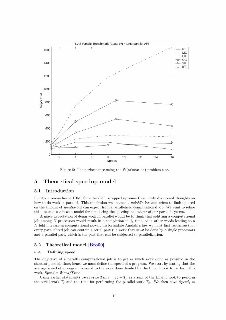
The next area of investigation is what type of problem runs well on our cluster. We choosethe W(orkstation) problem size and run the six benchmarks again (see Figure 8). This providesus with a thumbprint of Grendel.
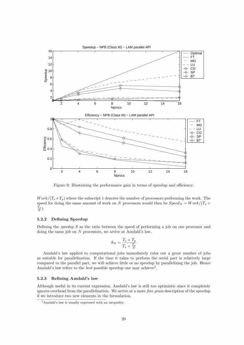
We expect that the kernel benchmarks, especially FT, will perform poorly on our architecture,because of the large communication overhead. This large communication overhead is due to the100 Mbps ethernet network, and the TCP/IP-stack in the Linux kernel. The network would bethe obvious choice of upgrade for boosting the performance of highly parallel applications. Figure8 suggests that the performance is poor for the kernel benchmarks, but let us analyze the resultsfurther. We use the speedup and efficiency measurements from section 4.1. In figure 9 we can seethe results from running the six benchmarks with the class W problem size.
4.3 Summary and conclusion of the benchmark results
The first objective of our benchmarks was to find out which implementation of MPI is most useful.Both LAM and MPICH implement the same MPI standard. The LAM approach of a user-leveldaemon controlling message communication and the use of only UDP-packets results in the bestperformance. The larger messages we try to send from MPI the higher bandwidth we get. Peakperformance is at about 80 kB data (1000 doubles) per message.
We also conclude that high network traffic between nodes doesn’t affect overall network per-formance.
Looking at the speedup (Figure 9) we find that the application benchmarks perform better thankernel benchmarks, and this becomes evident when we look at the efficiency. FT is approachingzero efficiency already at sixteen processors. MG and CG are not performing much better. Insection 6.1 we’ll see that a typical application at the Department of Scientific Computing, the socalled adveq problem, may be seen as an application benchmark and runs very well on Grendel.We can now deduce that a mix between computations and communication, where communicationis kept to a minimum is the key to achieving high performance for parallel applications.
18
2 4 6 8 10 12 14 160
200
400
600
800
1000
1200
1400
1600
NAS Parallel Benchmark (Class W) − LAM parallel API
Nprocs
Mop
/s to
tal
FTMGLUCGSPBT
Figure 8: The performance using the W(orkstation) problem size.
5 Theoretical speedup model
5.1 Introduction
In 1967 a researcher at IBM, Gene Amdahl, wrapped up some then newly discovered thoughts onhow to do work in parallel. This conclusion was named Amdahl’s law and refers to limits placedon the amount of speedup one can expect from a parallelized computational job. We want to refinethis law and use it as a model for simulating the speedup behaviour of our parallel system.
A naive expectation of doing work in parallel would be to think that splitting a computationaljob among N processors would result in a completion in 1
N time, or in other words leading to aN -fold increase in computational power. To formulate Amdahl’s law we must first recognize thatevery parallelized job can contain a serial part (i e work that must be done by a single processor)and a parallel part, which is the part that can be subjected to parallelization.
5.2 Theoretical model [Bro00]
5.2.1 Defining speed
The objective of a parallel computational job is to get as much work done as possible in theshortest possible time, hence we must define the speed of a program. We start by stating that theaverage speed of a program is equal to the work done divided by the time it took to perform thiswork, Speed = Work/T ime.
Using earlier statements we rewrite Time = Ts + Tp as a sum of the time it took to performthe serial work Ts and the time for performing the parallel work Tp. We then have Speed1 =
19
2 4 6 8 10 12 14 16
2
4
6
8
10
12
14
16Speedup − NPB (Class W) − LAM parallel API
Nprocs
Spe
edup
OptimalFT MG LU CG SP BT
2 4 6 8 10 12 14 160
0.2
0.4
0.6
0.8
1Efficiency − NPB (Class W) − LAM parallel API
Nprocs
Effi
cien
cy
FTMGLUCGSPBT
Figure 9: Illustrating the performance gain in terms of speedup and efficiency.
Work/(Ts+Tp) where the subscript 1 denotes the number of processors performing the work. Thespeed for doing the same amount of work on N processors would then be SpeedN = Work/(Ts +TpN ).
5.2.2 Defining Speedup
Defining the speedup S as the ratio between the speed of performing a job on one processor anddoing the same job on N processors, we arrive at Amdahl’s law.
SN =Ts + Tp
Ts + TpN
Amdahl’s law applied to computational jobs immediately rules out a great number of jobsas suitable for parallelization. If the time it takes to perform the serial part is relatively largecompared to the parallel part, we will achieve little or no speedup by parallelizing the job. HenceAmdahl’s law refers to the best possible speedup one may achieve3.
5.2.3 Refining Amdahl’s law
Although useful in its current expression, Amdahl’s law is still too optimistic since it completelyignores overhead from the parallelization. We arrive at a more fine grain description of the speedupif we introduce two new elements in the formulation.
3Amdahl’s law is usually expressed with an inequality.
20
Tis The average serial time that is spent on communication in various ways. This time probablydepends on the number of processors in some way. A suitable first approximation would bethat it is proportional to the number of processors.
Tip The average parallel time (that could be just idle time) when doing communication.
Using these definitions we end up with a better4 estimate for the speedup achieved throughparallelization.
SN =Ts + Tp
Ts +N × Tis + TpN + Tip
We still need to determine how to calculate Ts, Tis, Tp and Tip, and we do this by rewritingthe variables as:
Ts = OPs × top Where OPs is the number of arithmetic operations performed in the serial part,and top is the average time it takes to perform an arithmetic operation.
Tis = MPIs × tmpi Where MPIs is the number of doubles sent in the serial part. The variabletmpi is then the average time to send a double with the MPI interface.
Tp = OPp × top OPp is the number of arithmetic operations performed in the parallel part.
Tip = MPIp × tmpi And finallyMPIp which is the number of doubles sent with the MPI interfacein the parallel part of the program.
The speedup model (Equation (4))
SN =(OPs +OPp)top
OPs top +N(MPIs tmpi) + (OPp top)/N +MPIp tmpi(4)
is the model used in our simulations.
5.3 Model verification
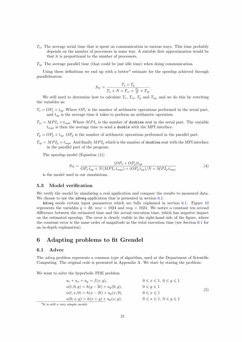
We verify the model by simulating a real application and compare the results to measured data.We choose to use the adveq-application that is presented in section 6.1.
Adveq needs certain input parameters which are fully explained in section 6.1. Figure 10represents the variables q = 20, nnx = 1024 and nny = 1024. We notice a constant ten seconddifference between the estimated time and the actual execution time, which has negative impacton the estimated speedup. The error is clearly visible in the right-hand side of the figure, wherethe constant error is the same order of magnitude as the total execution time (see Section 6.1 foran in-depth explanation).
6 Adapting problems to fit Grendel
6.1 Advec
The adveq problem represents a common type of algorithm, used at the Department of ScientificComputing. The original code is presented in Appendix A. We start by stating the problem:
We want to solve the hyperbolic PDE problem
ut + ux + uy = f(x, y), 0 6 x 6 1, 0 6 y 6 1u(t, 0, y) = h(y − 2t) + up(0, y), 0 6 y 6 1u(t, x, 0) = h(x− 2t) + up(x, 0), 0 6 x 6 1u(0, x, y) = h(x+ y) + up(x, y), 0 6 x 6 1, 0 6 y 6 1
(5)
4It is still a very simple model.
21
2 4 6 8 10 12 14 16
2
4
6
8
10
12
14
16
Number of processors
Spe
edup
OptimalModel Adveq
2 4 6 8 10 12 14 160
200
400
600
800
1000
Number of processors
Exe
c. ti
me
(s)
ModelAdveq
Figure 10: A verification of the model using the adveq-code presented in section 6.1
where
f(x, y) = 2ex+y + 3x2 + 6y2 + sin(x+ y
2
)+ cos
(x+ y
2
)up(x, y) = ex+y + x3 + 2y3 + sin
(x+ y
2
)− cos
(x+ y
2
)h(z) = sin (2πz)
The PDE problem (5) has the solution
u(t, x, y) = h(x+ y − 2t) + up(x, y) (6)
Here, we will solve the problem numerically by introducing the leap-frog scheme
un+1i,j + 2∆t(fi,j −D0xu
ni,j −D0yu
ni,j)
where
D0x =uni+1,j − uni−1,j
2∆x, D0y =
uni,j+1 − uni,j−1
2∆y
For simplicity, we’ll use the analytical solution (6) on the boundaries.The computational area is divided into an nnx by nny grid. Due to stability restrictions, the
total amount of timesteps is set to Nt = (nnx − 1) + (nny − 1). The grid is cut in the columndimension so that each processor gets a stripe of (approximately) the same width as the others.MPI is used for the message passing procedure. To make it possible to experiment with thecommunication-computation ratio, we have a parameter q which decides how many of a stripe’s
22
outermost columns are to be sent to the adjacent stripes. Sending data in larger chunks saves timespent on communicational start-ups. On the other hand, increasing q also increases computationalwork, since the same data somtimes is calculated on two processors. Note also that increasing qdoes not affect the total amount of data that is to be sent.
Initially the size of the problem and the parameter q are distributed to all processors. Thefirst two timesteps are calculated from the analytical solution. This is due to the finite differencestencil, which needs two layers5 to compute a third. After this, work is done on each processor inprimarily three steps :
repeat Nt/q times
1. Send the q outermost columns on each side of the stripe to the adjacent processors,respectively. This is done for the newest and the middle layer.
repeat steps 2 and 3 q times
2. Phase out the oldest layer, then set the middle layeras the oldest. Then set the newestlayer as the middle, leaving space for the new layer.
3. Calculate the new layer. For each turn in the inner loop, the calculated layer will bethinner and thinner, since there’s no communication going on. After q turns we willend up with a stripe of the initial width. Go back to step 1 and widen the stripe.
To estimate the time consumption we count which and how many operations are performed ineach step :
1. q columns are sent in eight steps (even-numbered and odd-numbered processors, send andreceive, u and unew). This is done Nt/q times. Time consumption : Nt/q∗8(ts+q∗nnx∗tw)
2. Pointers are easily shifted. We approximate this with zero work.
3. Since the work is somewhat unbalanced (the difference is however minor) we consider amiddle stripe. The outer loop is performed Nt/q times. The inner is performed q times. Inthe first turn of the inner loop, the overhead is 2(q − 1) columns (q − 1 on each side). Thenext turn, the overhead is 2(q−2) a s o. In total there are 2∗0.5∗q(q−1) overhead columnsin the inner loop. Add to that the q ∗ nny/size columns in the original stripe. In total wehave on each node
Number of elements = Nt/q ∗ nnx ∗ (2 ∗ 0.5 ∗ q(q − 1) + q ∗ nny/size)= Nt ∗ nnx((q − 1) + nny/size)
where size is the number of processors used.How many floating point operations are required on each element is not easily estimated,
especially since there are exponential and trigonometric function calls. There’s also main memoryfetches involved. The easiest is to make a test program that measures the time to operate on oneelement. This is done in Appendix C. The test program yields that operating on one elementconsumes approximately 430 ns. Let top = 430 ns. For ts and tw we use the results from ourping-pong program (see Appendix D), ts = 62µs and tw = 750ns. We now have
Total time = Nt(4(ts/q + nnx ∗ tw) + nnx((q − 1) + nny/size)top) (7)
if the number of processors is equal or greater than three. In the case of one or two processors thetotal time is reduced to
Total time for one processor = Nt ∗ nnx ∗ nny ∗ topTotal time for two processors = Nt(4(ts/q + nnx ∗ tw) + nnx(0.5 ∗ (q − 1) + nny/size)top)
23
0 2 4 6 8 10 12 14 160
100
200
300
400
500
600
700
800
900
1000
Number of processors
Exe
cutio
n tim
e (s
)
Adveq, gridsize 1024x1024
Experiment, q=1Theory, q=1Experiment, q=20Theory, q=20
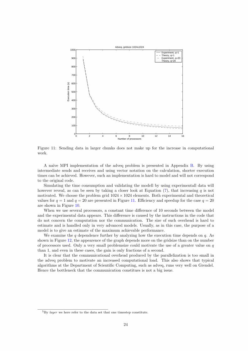
Figure 11: Sending data in larger chunks does not make up for the increase in computationalwork.
A naıve MPI implementation of the adveq problem is presented in Appendix B. By usingintermediate sends and receives and using vector notation on the calculation, shorter executiontimes can be achieved. However, such an implementation is hard to model and will not correspondto the original code.
Simulating the time consumption and validating the modell by using experimentall data willhowever reveal, as can be seen by taking a closer look at Equation (7), that increasing q is notmotivated. We choose the problem grid 1024× 1024 elements. Both experimental and theoreticalvalues for q = 1 and q = 20 are presented in Figure 11. Efficiency and speedup for the case q = 20are shown in Figure 10.
When we use several processors, a constant time difference of 10 seconds between the modeland the experimental data appears. This difference is caused by the instructions in the code thatdo not concern the computation nor the communication. The size of such overhead is hard toestimate and is handled only in very advanced models. Usually, as in this case, the purpose of amodel is to give an estimate of the maximum achievable performance.
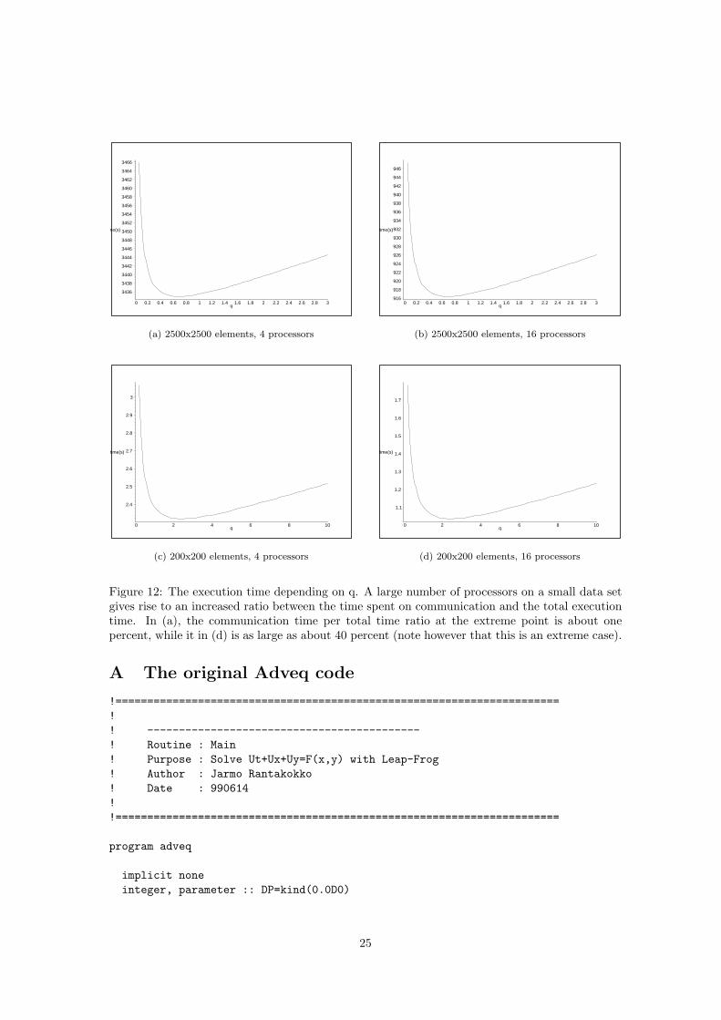
We examine the q dependence further by analyzing how the execution time depends on q. Asshown in Figure 12, the appearence of the graph depends more on the gridsize than on the numberof processors used. Only a very small problemsize could motivate the use of a greater value on qthan 1, and even in these cases, the gain is only fractions of a second.
It is clear that the communicational overhead produced by the parallelization is too small inthe adveq problem to motivate an increased computational load. This also shows that typicalalgorithms at the Department of Scientific Computing, such as adveq, runs very well on Grendel.Hence the bottleneck that the communication constitues is not a big issue.
5By layer we here refer to the data set that one timestep constitute.
24
3436
3438
3440
3442
3444
3446
3448
3450
3452
3454
3456
3458
3460
3462
3464
3466
time(s)
0 0.2 0.4 0.6 0.8 1 1.2 1.4 1.6 1.8 2 2.2 2.4 2.6 2.8 3q
(a) 2500x2500 elements, 4 processors
916
918
920
922
924
926
928
930
932
934
936
938
940
942
944
946
time(s)
0 0.2 0.4 0.6 0.8 1 1.2 1.4 1.6 1.8 2 2.2 2.4 2.6 2.8 3q
(b) 2500x2500 elements, 16 processors
2.4
2.5
2.6
2.7
2.8
2.9
3
time(s)
0 2 4 6 8 10q
(c) 200x200 elements, 4 processors
1.1
1.2
1.3
1.4
1.5
1.6
1.7
time(s)
0 2 4 6 8 10q
(d) 200x200 elements, 16 processors
Figure 12: The execution time depending on q. A large number of processors on a small data setgives rise to an increased ratio between the time spent on communication and the total executiontime. In (a), the communication time per total time ratio at the extreme point is about onepercent, while it in (d) is as large as about 40 percent (note however that this is an extreme case).
A The original Adveq code
!======================================================================!! -------------------------------------------! Routine : Main! Purpose : Solve Ut+Ux+Uy=F(x,y) with Leap-Frog! Author : Jarmo Rantakokko! Date : 990614!!======================================================================
program adveq
implicit noneinteger, parameter :: DP=kind(0.0D0)
25
!-- Variables.integer :: Nx,Ny,Nt,i,j,k,nthreadsreal(kind=DP) :: dt,dx,dy,norm,T,x,y,v,tireal(kind=DP)::ttime,ctime,walltimereal(kind=DP),pointer,dimension(:,:)::uold,u,unew,temp;
real(kind=DP)::F,up,hinteger omp_get_max_threadsinteger,parameter:: disk=10character(len=*),parameter :: input=’/home/da/adveq/original/params.dat’
!----------------------------------------------------------------------
ttime=walltime()! Set up the problemnamelist /problemsize/ Nx,Ny,nthreadsopen(unit=disk,file=input)read(disk,problemsize)close(disk)
! call omp_set_num_threads(nthreads)dx=1.0_DP/Nx; dy=1.0_DP/Ny; dt=1.0_DP/(Nx+Ny); T=1.0; Nt=nint(T/dt);allocate(uold(0:Nx,0:Ny),u(0:Nx,0:Ny),unew(0:Nx,0:Ny))
write(*,*) ’============================================’write(*,*) ’Version : Fortran 90’
! write(*,’(A,I8)’) ’ Number of threads:’,omp_get_max_threads()write(*,’(A,3I8)’) ’ Problem Size :’,Nx+1,Ny+1,Ntwrite(*,*) ’============================================’write(*,*) ’Computing...’
! Initial conditions!$OMP PARALLEL DO PRIVATE(i,j,x,y)do j=0,Ny
do i=0,Nxx=real(i,kind=DP)/Nx; y=real(j,kind=DP)/Nyu(i,j)=h(x+y)+up(x,y);unew(i,j)=h(x+y-2*dt)+up(x,y);
end doend do
!$OMP END PARALLEL DO
! Integrate the solution in timectime=walltime()do k=2,Nt
! Swap pointerstemp=>uold; uold=>u; u=>unew; unew=>temp;
! Leap Frog!$OMP PARALLEL!$OMP DO private(i,x,y)
do j=1,Ny-1do i=1,Nx-1
26
x=real(i,kind=DP)/Nx; y=real(j,kind=DP)/Nyunew(i,j)=uold(i,j)+2*dt*(F(x,y)- &
((u(i+1,j)-u(i-1,j))/2.0_DP*Nx+ &(u(i,j+1)-u(i,j-1))/2.0_DP*Ny))
end doend do
!$OMP END DO NOWAIT
! Boundary conditionsti=k*dt;
!$OMP DO private(y)do j=0,Ny
y=real(j,kind=DP)*dyunew(0,j)=h(y-2*ti)+up(0.0_DP,y)
end do!$OMP END DO NOWAIT!$OMP DO private(x)
do i=1,Nxx=real(i,kind=DP)*dxunew(i,0)=h(x-2*ti)+up(x,0.0_DP)
end do!$OMP END DO NOWAIT
!Exact boundary conditionsx=1.0_DP
!$OMP DO private(y)do j=1,Ny
y=real(j,kind=DP)*dyunew(Nx,j)=up(x,y)+h(x+y-2*ti)
end do!$OMP END DO NOWAIT
y=1.0_DP!$OMP DO private(x)
do i=1,Nx-1x=real(i,kind=DP)*dxunew(i,Ny)=up(x,y)+h(x+y-2*ti)
end do!$OMP END DO NOWAIT!$OMP END PARALLEL
end doctime=walltime()-ctime
! Residual norm || u_new-(h(x+y-2*t)+up(x,y)) ||norm=0.0
!$OMP PARALLEL DO PRIVATE(i,x,y,v) REDUCTION(+:norm)do j=0,Ny
do i=0,Nxx=real(i,kind=DP)/Nx; y=real(j,kind=DP)/Nyv=h(x+y-2*Nt*dt)+up(x,y)norm=norm+(unew(i,j)-v)*(unew(i,j)-v);
end doend do
!$OMP END PARALLEL DO
27
ttime=walltime()-ttime! Display results
write(*,*) ’--------------’write(*,’(A,F9.4,A)’) ’ Total time : ’,ttime,’ sec’write(*,’(A,F9.4,A)’) ’ Compute time : ’,ctime,’ sec’write(*,’(A,E14.6)’) ’ Error norm : ’,norm/sqrt(real(Nx*Ny))write(*,*) ’--------------’
end program adveq
B The MPI implementation of the Adveq code
program adveq
implicit none
include ’mpif.h’
integer, parameter :: DP=kind(0.0D0)
integer :: Nx,Ny,Nt,i,j,k,nthreads,q,q1integer :: nnx,nny,nx1,nx2,ny1,ny2,restreal(kind=DP) :: dt,dx,dy,mynorm,norm,T,x,y,v,tireal(kind=DP) :: ttime,ctime,walltimereal(kind=DP),pointer,dimension(:,:) :: uold,u,unew,temp
real(kind=DP) :: F,up,h ! Functionsinteger,parameter :: disk=10character(len=*),parameter :: input=’/home/da/adveq/p1/params.dat’
integer :: rank,size,ierrorinteger, dimension(3) :: tmpbuf
ttime = walltime()
! Initialize MPI, find out my rank and how many procs are usedcall MPI_INIT(ierror)call MPI_COMM_SIZE(MPI_COMM_WORLD,size,ierror)call MPI_COMM_RANK(MPI_COMM_WORLD,rank,ierror)
! Distribute problem dimensionsif(rank .eq. 0) then
namelist /problemsize/ Nx,Ny,qopen(unit=disk,file=input)read(disk,problemsize)close(disk)
tmpbuf(1) = Nxtmpbuf(2) = Nytmpbuf(3) = q
28
write(*,*) ’============================================’write(*,*) ’Version : Fortran 90’write(*,’(A,I8)’) ’ Number of threads:’,rankwrite(*,’(A,3I8)’) ’ Problem Size :’,Nx+1,Ny+1,Ntwrite(*,*) ’============================================’write(*,*) ’Computing...’
end if
call MPI_BCAST(tmpbuf,3,MPI_INTEGER,0,MPI_COMM_WORLD,ierror)
if(rank .ne. 0) then
Nx = tmpbuf(1)Ny = tmpbuf(2)q = tmpbuf(3)
end if
dx=1.0_DP/Nx; dy=1.0_DP/Ny; dt=1.0_DP/(Nx+Ny); T=1.0; Nt=nint(T/dt);
! Calculate local boundaries and allocate arraysnnx=(Nx+1); nny=(Ny+1)/size; rest=mod((Ny+1),size);nx1=0; nx2=nnx-1;if(rest .gt. rank) then
nny=nny+1;ny1=nny*rank; ny2=ny1+nny-1;
elseny1=rest*(nny+1)+(rank-rest)*nny;ny2=ny1+nny-1;
end if
allocate( uold(0:nnx-1,ny1-q:ny2+q), u(0:nnx-1,ny1-q:ny2+q), &unew(0:nnx-1,ny1-q:ny2+q))
! Set initial conditionsdo j=ny1,ny2
do i=nx1,nx2x=real(i,kind=DP)/Nx; y=real(j,kind=DP)/Nyu(i,j)=h(x+y)+up(x,y)unew(i,j)=h(x+y-2*dt)+up(x,y)!u(i,j)=rank+1000!unew(i,j)=rank+1000
end doend do
! Integrate in timectime = walltime()do k=0,(Nt-2)/q
! Send data in every q:th timestep
29
! u
! Even-numbered procs send to the right and the others receive! from the left and the other way aroundif(rank .ne. size-1 .and. mod(rank,2) .eq. 0) then
call MPI_SEND(u(:,ny2-q+1:ny2),q*nnx,MPI_DOUBLE_PRECISION,&rank+1,1001,MPI_COMM_WORLD)
call MPI_RECV(u(:,ny2+1:ny2+q),q*nnx,MPI_DOUBLE_PRECISION,&rank+1,1002,MPI_COMM_WORLD)
else if(rank .ne. 0 .and. mod(rank,2) .eq. 1) thencall MPI_RECV(u(:,ny1-q:ny1-1),q*nnx,MPI_DOUBLE_PRECISION,&rank-1,1001,MPI_COMM_WORLD)
call MPI_SEND(u(:,ny1:ny1+q-1),q*nnx,MPI_DOUBLE_PRECISION,&rank-1,1002,MPI_COMM_WORLD)
end if
! Odd-numbered procs send to the right and the others receive! from the left.if(rank .ne. size-1 .and. mod(rank,2) .eq. 1) then
call MPI_SEND(u(:,ny2-q+1:ny2),q*nnx,MPI_DOUBLE_PRECISION,&rank+1,1003,MPI_COMM_WORLD)
call MPI_RECV(u(:,ny2+1:ny2+q),q*nnx,MPI_DOUBLE_PRECISION,&rank+1,1004,MPI_COMM_WORLD)
else if(rank .ne. 0 .and. mod(rank,2) .eq. 0) thencall MPI_RECV(u(:,ny1-q:ny1-1),q*nnx,MPI_DOUBLE_PRECISION,&rank-1,1003,MPI_COMM_WORLD)
call MPI_SEND(u(:,ny1:ny1+q-1),q*nnx,MPI_DOUBLE_PRECISION,&rank-1,1004,MPI_COMM_WORLD)
end if
! unew
! Even-numbered procs send to the right and the others receive! from the left.if(rank .ne. size-1 .and. mod(rank,2) .eq. 0) then
call MPI_SEND(unew(:,ny2-q+1:ny2),q*nnx,MPI_DOUBLE_PRECISION,&rank+1,1005,MPI_COMM_WORLD)
call MPI_RECV(unew(:,ny2+1:ny2+q),q*nnx,MPI_DOUBLE_PRECISION,&Rank+1,1006,MPI_COMM_WORLD)
else if(rank .ne. 0 .and. mod(rank,2) .eq. 1) thencall MPI_RECV(unew(:,ny1-q:ny1-1),q*nnx,MPI_DOUBLE_PRECISION,&rank-1,1005,MPI_COMM_WORLD)
call MPI_SEND(unew(:,ny1:ny1+q-1),q*nnx,MPI_DOUBLE_PRECISION,&rank-1,1006,MPI_COMM_WORLD)
end if
! Odd-numbered procs send to the right and the others receive! from the left.if(rank .ne. size-1 .and. mod(rank,2) .eq. 1) then
call MPI_SEND(unew(:,ny2-q+1:ny2),q*nnx,MPI_DOUBLE_PRECISION,&rank+1,1007,MPI_COMM_WORLD)
call MPI_RECV(unew(:,ny2+1:ny2+q),q*nnx,MPI_DOUBLE_PRECISION,&rank+1,1008,MPI_COMM_WORLD)
else if(rank .ne. 0 .and. mod(rank,2) .eq. 0) then
30
call MPI_RECV(unew(:,ny1-q:ny1-1),q*nnx,MPI_DOUBLE_PRECISION,&rank-1,1007,MPI_COMM_WORLD)
call MPI_SEND(unew(:,ny1:ny1+q-1),q*nnx,MPI_DOUBLE_PRECISION,&rank-1,1008,MPI_COMM_WORLD)
end if
! Calculate q timesteps
do q1=q-1,0,-1
temp=>uold; uold=>u; u=>unew; unew=>temp
ti = (k*q+(q-q1-1)+2)*dt
! Take care of special case size=1if(size .eq. 1) then
do j=ny1+1,ny2-1do i=nx1+1,nx2-1
x=real(i,kind=DP)*dx; y=real(j,kind=DP)*dyunew(i,j)=uold(i,j)+2*dt*(F(x,y)- &
((u(i+1,j)-u(i-1,j))/2.0_DP*Nx+ &(u(i,j+1)-u(i,j-1))/2.0_DP*Ny))
end doend do! Left boundary (use exact solution)do i=nx1+1,nx2-1
x=real(i,kind=DP)*dxunew(i,0)=h(x-2*ti)+up(x,0.0_DP)
end do! Right boundary (use exact solution)do i=nx1+1,nx2-1
x=real(i,kind=DP)*dxunew(i,Ny)=h(x+1.0_DP-2*ti)+up(x,1.0_DP)
end do
! Take care of leftmost stripeelse if(rank .eq. 0) then
do j=1,ny2+q1do i=nx1+1,nx2-1
x=real(i,kind=DP)*dx; y=real(j,kind=DP)*dyunew(i,j)=uold(i,j)+2*dt*(F(x,y)- &
((u(i+1,j)-u(i-1,j))/2.0_DP*Nx+ &(u(i,j+1)-u(i,j-1))/2.0_DP*Ny))
end doend do! Left boundary (use exact solution)do i=nx1+1,nx2-1
x=real(i,kind=DP)*dxunew(i,0)=h(x-2*ti)+up(x,0.0_DP)
end do
! Take care of rightmost stripeelse if(rank .eq. size-1) then
do j=ny1-q1,ny2-1
31
do i=nx1+1,nx2-1x=real(i,kind=DP)*dx; y=real(j,kind=DP)*dyunew(i,j)=uold(i,j)+2*dt*(F(x,y)- &
((u(i+1,j)-u(i-1,j))/2.0_DP*Nx+ &(u(i,j+1)-u(i,j-1))/2.0_DP*Ny))
end doend do! Right boundary (use exact solution)do i=nx1+1,nx2-1
x=real(i,kind=DP)*dxunew(i,Ny)=h(x+1.0_DP-2*ti)+up(x,1.0_DP)
end do
! Take care of middle stripe(s)else
do j=ny1-q1,ny2+q1do i=nx1+1,nx2-1
x=real(i,kind=DP)*dx; y=real(j,kind=DP)*dyunew(i,j)=uold(i,j)+2*dt*(F(x,y)- &
((u(i+1,j)-u(i-1,j))/2.0_DP*Nx+ &(u(i,j+1)-u(i,j-1))/2.0_DP*Ny))
end doend do
end if
! Top boundary (use exact solution)do j=ny1-q1,ny2+q1
y=real(j,kind=DP)*dyunew(0,j)=h(y-2*ti)+up(0.0_DP,y)
end do! Bottom boundary (use exact solution)do j=ny1-q1,ny2+q1
y=real(j,kind=DP)*dyunew(Nx,j)=h(1.0_DP+y-2*ti)+up(1.0_DP,y)
end do
end doend doctime = walltime()-ctime
! Calculate error normmynorm=0.0do j=ny1,ny2
do i=nx1,nx2x=real(i,kind=DP)*dx; y=real(j,kind=DP)*dyv=h(x+y-2*ti)+up(x,y)mynorm=mynorm+(unew(i,j)-v)*(unew(i,j)-v)
end doend do
call MPI_REDUCE(mynorm,norm,1,MPI_DOUBLE_PRECISION,MPI_SUM,0,&MPI_COMM_WORLD)
ttime = walltime()-ttimeif(rank .eq. 0) then
32
! Display resultswrite(*,*) ’--------------’write(*,’(A,F9.4,A)’) ’ Total time : ’,ttime,’ sec’write(*,’(A,F9.4,A)’) ’ Compute time : ’,ctime,’ sec’write(*,’(A,E14.6)’) ’ Error norm : ’,norm/sqrt(real(Nx*Ny))write(*,*)’End time :’,tiwrite(*,*) ’--------------’
end if
deallocate(uold,u,unew)call MPI_FINALIZE(ierror)
end program adveq
C Additional files to the Adveq application
params.dat :
&problemsizeNx= 1024,Ny= 1024,nthreads=1
&end
force.f :
function h(z)integer, parameter :: DP=kind(0.0D0)real(kind=DP):: z,hreal(kind=DP),parameter :: twopi=6.28318530717959_DPh=sin(twopi*z)
end function h
function F(x,y)integer, parameter :: DP=kind(0.0D0)real(kind=DP):: F,x,yF=2*exp(x+y)+3*x*x+6*y*y+sin((x+y)/2)+cos((x+y)/2)
end function F
function up(x,y)integer, parameter :: DP=kind(0.0D0)real(kind=DP):: up,x,yup=exp(x+y)+x*x*x+2*y*y*y+sin((x+y)/2)-cos((x+y)/2)
end function up
mpi.f :
module mpiimplicit noneinclude ’lam.h’
end module mpi
walltime.f :
33
function walltime()integer, parameter:: DP = kind(0.0D0)real(DP) walltimeinteger::count,count_rate,count_maxcall system_clock(count,count_rate,count_max)walltime=real(count,DP)/real(count_rate,DP)
end function walltime
D The modified ping-pong program to measure network-traffic
/*********************************************************************** Will toss a message (1000 doubles) back and forth between two* processors in a tight loop 100000 times** This is an example of persistent communication in MPI/C** Andreas Khri* 1999-12-30 (new years eve tomorrow)**********************************************************************/
#include <mpi.h>#include <stdio.h>#include <stdlib.h>
int main(int argc, char *argv[]) {int rank, size, i;char message[4200];double timer1, timer2;MPI_Request pingreq, pongreq;char namn[255];FILE *utfil;FILE *infil;char buff[255];
MPI_Init(&argc, &argv); /* Initialize MPI */
MPI_Comm_size(MPI_COMM_WORLD, &size); /* Get the number of processors */MPI_Comm_rank(MPI_COMM_WORLD, &rank); /* Get my number */
sprintf(namn, "/home/kja/pingpong/re%d", rank); /* save the answer for eachprocessor on a sharedfilearea (home dir) */
if (size != 2) { /* This if-block makes sure only two processors* takes part in the execution of the code, pay no* attention to it */
if (rank == 0)fprintf(stderr, "\aRun on two processors only!\n");
MPI_Finalize();exit(0);
34
}
/* ’pingreq’ will hold the request for processor 0 to send and for* processor 1 to receive** ’pongreq’ will hold the request for processor 0 to receive and* for processor 1 to send */
if (rank == 0) {MPI_Send_init(message, 4000, MPI_CHAR, 1, 111, MPI_COMM_WORLD, &pingreq);MPI_Recv_init(message, 4000, MPI_CHAR, 1, 222, MPI_COMM_WORLD, &pongreq);
} else {MPI_Recv_init(message, 4000, MPI_CHAR, 0, 111, MPI_COMM_WORLD, &pingreq);MPI_Send_init(message, 4000, MPI_CHAR, 0, 222, MPI_COMM_WORLD, &pongreq);
}
/* save kernel information found in /proc/net/dev to a filefor manual verification */
utfil=fopen(namn, "w+");if(utfil) {fprintf(utfil, "Fore:\n");infil=fopen("/proc/net/dev", "r");if(infil) {while(!feof(infil)) {
memset(buff, 0, 255);fread(buff, 255, 1, infil);fwrite(buff, 255,1, utfil);
}}fclose(infil);fclose(utfil);
}
timer1 = MPI_Wtime(); /* Time the tight loop */
for (i = 0; i < 100000; i++) { /* This is the tight loop */MPI_Status status;
MPI_Start(&pingreq); /* Send/recv in one direction */MPI_Wait(&pingreq, &status); /* Wait for completion */
MPI_Start(&pongreq); /* Send/recv in the other direction */MPI_Wait(&pongreq, &status); /* Wait for completion */
}
timer1 = MPI_Wtime() - timer1; /* Get the final elapsed wallclocktime for the tight loop */
/* save kernel information again to compare with previous data */utfil=fopen(namn, "a+");if(utfil) {fprintf(utfil, "Efter:\n");infil=fopen("/proc/net/dev", "r");if(infil) {
35
while(!feof(infil)) {memset(buff, 0, 255);fread(buff, 255, 1, infil);fwrite(buff, 255,1, utfil);
}}fclose(infil);fclose(utfil);
}
/* Now, sum the two elapsed times in processor 0 */MPI_Reduce(&timer1, &timer2, 1, MPI_DOUBLE, MPI_SUM, 0, MPI_COMM_WORLD);
if (rank == 0)/* Print the mean time */printf("Time per iteration = %.16f\n", 0.5*timer2/100000.0);
MPI_Finalize(); /* Shut down and clean up */
return 0;}
E A program to measure networktraffic
/*************************************************** Simple program to get exact network traffic* Reads network counters in the Linux kernel* to measure nr of bytes and packets sent and* transmitted for eth0.* Uses temporary file /tmp/.trafik**************************************************/
#include <stdio.h>#include <stdlib.h>#include <time.h>
int main(int argc, char *argv[]) {time_t t1, t2;FILE * utfil;FILE *infil;char buff[255];char * pek;unsigned long rp1, rp2, tp1, tp2, rb1, rb2, tb1, tb2;unsigned long s1, s2, s5;double d1, d2, d3, d4;s5=24;utfil=fopen("/tmp/.trafik", "r");if(utfil) {fread(&t2, 1, sizeof(t1), utfil);fread(&rb2, 1, sizeof(rp1), utfil);fread(&rp2, 1, sizeof(rp1), utfil);fread(&tb2, 1, sizeof(rp1), utfil);fread(&tp2, 1, sizeof(rp1), utfil);
36
s5=25;fclose(utfil);}else {fprintf(stderr, "Hittar inte /tmp/.trafik - skapar den\n");
}
/* get kernel-data from /proc/net/dev (requires kernel >=2.2) */utfil=fopen("/tmp/.trafik", "w+");infil=fopen("/proc/net/dev", "r");if(infil) {/* Skip 3 first lines of text /*memset(buff, 0, 255);fgets(buff, 255, infil);memset(buff, 0, 255);fgets(buff, 255, infil);memset(buff, 0, 255);fgets(buff, 255, infil);memset(buff, 0, 255);fgets(buff, 255, infil);pek=&(buff[7]); /* skip first 7 bytes */sscanf(pek, "%u %u %d %d %d %d %d %d %u %u", &rb1, &rp1, &s1, &s1, &s1, &s1, &s1,
&s1, &tb1, &tp1);}fclose(infil);
/* Save current time and current counters */t1=time(NULL);fwrite(&t1, 1, sizeof(t1), utfil);fwrite(&rb1, 1, sizeof(rp1), utfil);fwrite(&rp1, 1, sizeof(rp1), utfil);fwrite(&tb1, 1, sizeof(rp1), utfil);fwrite(&tp1, 1, sizeof(rp1), utfil);fclose(utfil);
/* Calculate differences if there are any */if(s5==25) {d1=(rp1-(double)rp2)/((double)t1-t2);d2=(rb1-(double)rb2)/((double)t1-t2);d3=(rb1-(double)rb2)/((double)rp1-rp2);printf("Tidsintervall: %d sekunder\n", t1-t2);printf("Recieve:\n");printf(" %u paket, %u bytes\n", rp1-rp2, rb1-rb2);printf(" %f paket/sek, %f bytes/s, %f bytes/paket\n", d1, d2, d3);d1=(tp1-(double)tp2)/((double)t1-t2);d2=(tb1-(double)tb2)/((double)t1-t2);d3=(tb1-(double)tb2)/((double)tp1-tp2);printf("Transmit:\n");printf(" %u paket, %u bytes\n", tp1-tp2, tb1-tb2);printf(" %f paket/sek, %f bytes/s, %f bytes/paket\n", d1, d2, d3);
}return 0;
}
37
References
[AMD00] AMD Athlon Processor Architecture. Report, Advanced Micro Devices, Inc., OneAMD Place, Sunnyvale, CA, 94088, 2000.
[BBB+94] D. Bailey, E. Barszcz, J. Barton, D. Browning, R. Carter, L. Dagum, R. Fatoohi,S. Fineberg, P. Fredrickson, T. Lasinski, R. Screiber, H. Simon, V. Venkatakrishnan,and S. Weeratunga. THE NAS PARALLEL BENCHMARKS. RNR Technical ReportRNR-94-007, NASA Ames Research Center, Mail Stop T27A-1, Moffet Field, CA,94035-1000, March 1994.
[BEO] www.beowulf.org. See http://www.beowulf.org for a full description of the beowulfproject, access to the beowulf mailing list, and more.
[BHS+95] David Bailey, Tim Harris, William Saphir, Rob van der Wijngaart, Alex Woo, andMaurice Yarrow. The NAS Parallel Benchmarks 2.0. Report NAS-95-020, NASA AmesResearch Center, Moffett Field, CA, 94035-1000, December 1995.
[Bro00] Robert G. Brown. Maximizing beowulf performance. Report, Duke Uni-versity Physics Department, Box 90305, Durham, NC, 27708-0305, 2000.http://www.phy.duke.edu/˜rgb.
[CLMR00] P.H. Carns, W.B. Ligon, S.P. McMillan, and R.B. Ross. An evaluation of message pass-ing implementations on beowulf workstations. Report, Parallell Arichtecture ResearchLab Clemson University, 102 Riggs Hall, Clemson, SC, 29634-0915, 2000. http://www-unix.mcs.anl.gov/˜rross/aero99/aero99.html.
[KGGK94] Vipin Kumar, Ananth Grama, Ansuhl Gupta, and George Karypis. Introduction toParallel Computing - Design and analysis of algorithms. The Benjamin/CummingsPublishing Company, Inc., 390 Bridge Parkway, Redwood City, CA, 94065, 1994.University of Minnesota.
[MPI95] MPI: A Message-Passing Interface Standard. Report, Message Passing Interface Fo-rum, 1995.
[MS96] Larry McVoy and Carl Staelin. lmbench: Portable tools for performance analysis.Technical report, Silicon Graphics, Inc. and Hewlett-Packard Laboratories, January1996. http://www.bitmover.com/lmbench/.
[NET96] Netperf: A Network Performance Benchmark, February 1996. Information NetworksDivision, Hewlett-Packard Company.
[RBM97] Daniel Ridge, Donald Becker, and Phillip Merkey. Beowulf: Harnessing the power ofparallelism in a pile-of-pcs. Technical report, IEEE Aerospace, 1997.
[SAR01] Some notes about BLAS, LAPACK, ATLAS and SCALAPACK. Seehttp://www.sara.nl/beowulf/lapackstory.html, 2001.
[SMG96] Quinn O. Snell, Armin R. Mikler, and John L. Gustafson. Netpipe: A network protocolindependent performance evaluator. Report, Ames Laboratory/Scalable ComputingLab, Ames, Iowa 50011, 1996. http://www.scl.ameslab.gov/netpipe/paper/full.html.
[St1] Jorgen Stadje. Beowulf ger LiU superprestanda. Natverk & kommunikation, (2), 2001.
38