an evaluation of a piezometer-based constant head

A D e p a r t m e n t o f E c o l o g y R e p o r t

An Evaluation of a Piezometer-Based Constant Head Injection Test (CHIT) for use in Groundwater/Surface Water Interaction Studies

Abstract

This paper presents an evaluation of Cardenas and Zlotnik’s piezometer-based, constant head injection test (CHIT) for estimating the hydraulic conductivity (K) of streambed and lake-bed sediments during studies of groundwater/surface water exchange. To provide experimental data for this evaluation, the CHIT was performed on 21 small-diameter, instream piezometers deployed in support of ongoing Washington State Department of Ecology (Ecology) Total Maximum Daily Load (water cleanup plan) studies. In addition to assessing the practical application of the test for future Ecology studies, a sensitivity analysis was completed to determine the influence of field measurement errors on the K estimate. The simplicity and speed of the test procedure can improve efforts to bracket the K variability of groundwater/surface water interface-zone sediments throughout a study area. Standardized operating procedures and recommendations are presented for future use of the CHIT in Ecology studies.

November 2006 (updated August 2007) Publication No. 06-03-042

Publication Information

This report is available on the Department of Ecology’s web site at www.ecy.wa.gov/biblio/0603042.html August 2007 update: The original version of this publication (November 2006) has been updated to reflect an erratum published for the Cardenas and Zlotnik (2003) reference. Several mathematical terms were also revised to provide consistency with that erratum. Author: Charles F. Pitz, L.G., L.HG. Washington State Department of Ecology Address: PO Box 47600, Olympia WA 98504-7600 E-mail: [email protected] Phone: (360) 407-6775 This report was prepared by a licensed hydrogeologist. A signed and stamped copy of the report is available upon request. For more information contact:

Publications Coordinator Environmental Assessment Program P.O. Box 47600 Olympia, WA 98504-7600

E-mail: [email protected]: (360) 407-6764

Any use of product or firm names in this publication is for descriptive purposes only and does not imply endorsement by the author or the Department of Ecology If you need this publication in an alternate format, call Joan LeTourneau at (360) 407-6764. Persons with hearing loss can call 711 for Washington Relay Service. Persons with a speech disability can call 877-833-6341.

http://www.ecy.wa.gov/biblio/0603042.html

mailto:[email protected]

mailto:[email protected]

Table of Contents

Page

Abstract ........................................................................................................................................... 1

Acknowledgements......................................................................................................................... 4

Introduction..................................................................................................................................... 5

Method ............................................................................................................................................ 6

Data Analysis .................................................................................................................................. 7 CHIT Model Equations............................................................................................................. 7 CHIT Model Assumptions........................................................................................................ 8

Experimental Data and Results....................................................................................................... 9

Sensitivity Analysis ...................................................................................................................... 10 Influence of Input Parameter Errors or Assumptions ............................................................. 10

Injection Rate .................................................................................................................... 10 Operating Head ................................................................................................................. 10 Screen Length ................................................................................................................... 12 Piezometer Depth/Incline ................................................................................................. 13 Partial Penetration............................................................................................................. 13 Effective Radius................................................................................................................ 13

Influence of Open Interval Area, Turbulence Effects, and Friction Loss............................... 14

Discussion and Recommendations ............................................................................................... 15

References..................................................................................................................................... 17

Appendix A. EAP Standard Operating Procedure for Constant Head Injection Tests (CHIT) for Small-Diameter Piezometers ............................................................................ 19

Appendix B. Study Data .............................................................................................................. 27

Appendix C. EAP Field Data Sheet for Constant Head Injection Test (CHIT) .......................... 31

Acknowledgements The author wishes to thank the Environmental Assessment Program colleagues who were helpful in the completion of this study. Brenda Nipp, Bryan Neet, and Scott Tarbutton provided invaluable field assistance. James Kardouni and Dustin Bilhimer provided piezometer construction and installation details, and Kirk Sinclair and Melanie Kimsey peer-reviewed the draft report. Nigel Blakley provided recommendations regarding statistical analysis of the study data. Joan LeTourneau provided editorial assistance during the preparation of the report. The author also benefited greatly from conversations with the original developers of the test method, Bayani Cardenas (New Mexico Tech) and Vitaly Zlotnik (University of Nebraska-Lincoln).

Introduction The Washington State Department of Ecology (Ecology) Environmental Assessment Program (EAP) has conducted a number of studies to characterize the interaction between groundwater and surface water. Many of these studies require the project hydrogeologist to develop a time-weighted volume estimate of water exchange between an aquifer system and an overlying surface stream, river, or lake. Flow analysis using Darcy’s law is one common method of calculating a volume flux across a groundwater/surface water interface. Darcy’s law (Freeze and Cherry, 1979; Fetter, 1980) states that the amount of water transmitted across an interface (or seepage face) can be expressed as:

Q = -KiA (1) where:

Q = the quantity of water transmitted across a interface per unit of time (volume/time) K = the hydraulic conductivity of the interface sediments (distance/time) i = the hydraulic gradient across the interface (dimensionless) A = the cross-sectional area of the interface (distance2) EAP hydrogeologists have been deploying numerous smaller diameter piezometers (≤ 1.5 inch) between 3 to 10 feet into stream and lake beds to directly measure the vertical hydraulic gradient for use in Equation 1. To calculate a flux value, these measurements can be integrated with (1) estimates of the surface area over which seepage occurs (for example, by measuring the wetted width and length of a stream reach), and (2) the permeability character of the sediments in the zone lying below the stream or lake bottom. Until recently, EAP staff have not had an efficient, field-based tool to estimate the hydraulic conductivity value of submerged streambed or lake-bed sediments. Past studies have extrapolated values from pumping test information from nearby wells, drawn on published literature values for sediments of similar character (e.g., Calver, 2001), or used time-intensive approaches such as modeling thermal data collected from thermistors deployed across the vertical axis of the interface zone (after methods described by authors such as Conant, 2004, and Wu et al., 2004). This paper evaluates the use of a field-based, hydraulic test method that allows rapid measurement of the permeability character of interface-zone sediments using the small diameter piezometers already being deployed by EAP for measurements of hydraulic gradient (and water quality). The goal of this evaluation was to determine if the test is practical for use in EAP studies, and to identify the key field-measurement factors influencing the hydraulic conductivity estimates derived from the test.

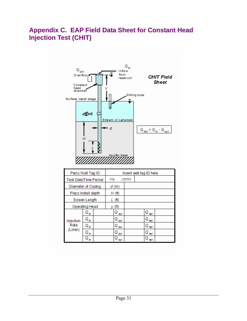
Method Cardenas and Zlotnik (2003) introduced procedures for conducting a constant head injection test (CHIT) on small diameter piezometers driven into a streambed. The data from the test can be used to estimate the hydraulic conductivity (K) value of the sediments located adjacent to the open interval of the piezometer. The CHIT method greatly simplifies the equipment and procedures required by previously published methods for field estimating sediment K in submerged settings (e.g., Kelly and Murdoch, 2003; Cho et al., 2000; Wilson et al., 1997; Landon et al., 2001; Leek, 2006). Figure 1 presents a schematic diagram of the CHIT apparatus.

Stilling tube

Qin

H

L

Aquifer base

y

Stream bed

Surface water stage

d

Inflow from reservoir

Constant head chamber

Qout Overflow

b

Qin - Qout = Qnet

Figure 1. Schematic Diagram of a Constant Head Injection Test (CHIT) Apparatus (modified from Cardenas and Zlotnik, 2003)

To conduct a CHIT, flow from an external water reservoir is injected into a screened piezometer casing at a rate that is in equilibrium with the ability of the aquifer sediments to ‘receive’ the injected water. Measurements of the equilibrated flow rate, and the operating head (y)(Figure 1) are then measured as accurately as possible1. These field measurements are integrated with details about the piezometer casing construction and installation depth to estimate an isotropic hydraulic conductivity of the sediments. Appendix A presents a standard operating procedure for the CHIT method using equipment assembled for this study. Data Analysis CHIT Model Equations Equation 2 presents the formula for estimating a hydraulic conductivity value (K) from the CHIT measurement data (Cardenas and Zlotnik, 2003)(Figure 1): K = Q (2) 2πLPy

where: K = the isotropic hydraulic conductivity of the interface-zone sediments (distance/time) Q = the net constant head injection rate (Qin-Qout) (volume/time) L = the total length of the open interval of the piezometer (distance) P = well shape factor (dimensionless) y = operating head; the height of the constant head above the stream or lake stage (distance) The well shape factor P can be estimated using Bouwer and Rice’s equation (Bouwer and Rice, 1976; Cardenas and Zlotnik, 2003; Butler, 1998)(Figure 1): P = 1.1 + A+B(ln[(b-(l+L))/ rw]) if H < b (3) ln((l+L)/ rw) L/ rw

or

P = 1.1 + C if H = b (4) ln((l+L)/ rw) L/ rw

where:

1 For a CHIT procedure, the operating head is the difference between the constant hydraulic head maintained inside the piezometer and the hydraulic head exerted on the groundwater/surface water interface (i.e., the stream or lake stage).

P = well shape factor l = the distance between the streambed surface and the top of the open interval of the piezometer (ft) L = the total length of the open interval of the piezometer (distance) H = the total depth of penetration of the piezometer below the streambed (l+L) (distance) rw = effective radius of the piezometer (distance) A,B, and C = empirical coefficients (dimensionless) L = the total length of the open interval of the piezometer (distance) b = the total saturated thickness of the aquifer (distance) The empirical coefficients A, B, and C can be estimated using Van Rooy’s polynomial functions (Van Rooy, 1988; Butler, 1998)(Figure 1): A = 1.4720 + 3.537 · 10-2(L/rw) – 8.148 · 10-5(L/rw)2 + 1.028 · 10-7(L/rw)3 – 6.484 · 10-11(L/rw)4 + 1.573 · 10-14(L/rw)5 (5) B = 0.2372 + 5.151 · 10-3(L/rw) – 2.682 · 10-6(L/rw)2 – 3.491 · 10-10(L/rw)3 + 4.738 · 10-13(L/rw)4 (6) C = 0.7920 + 3.993 · 10-2(L/rw) – 5.743 · 10-5(L/rw)2 + 3.858 · 10-8(L/rw)3 – 9.659 · 10-12(L/rw)4 (7)

where: A, B = empirical coefficients for partially penetrating piezometers (dimensionless) C = an empirical coefficient for fully penetrating piezometers (dimensionless) L = the total length of the open interval of the piezometer (distance) rw = effective radius of the piezometer (distance) CHIT Model Assumptions The data analysis equations for the CHIT method assume: The aquifer base underlying the piezometer is an impermeable boundary.

Other than the piezometer open interval, the piezometer casing is impermeable.

The stream stage exerts a constant hydraulic head at the groundwater/surface water interface, and is undisturbed at a large distance from the piezometer screen.

Flow across the piezometer open interval is laminar, unaffected by turbulence or frictional head loss.

The interface-zone sediments being tested are hydraulically isotropic at the sub-meter scale, therefore the K estimate describes an isotropic condition (Cardenas and Zlotnik, 2003; Burger and Belitz, 1997; Izbicki, 2002).

The screened portion of the aquifer is fully saturated.

During the test, there is no vertical movement of the injected water up or down an annular space between the streambed sediments and the piezometer casing.

Experimental Data and Results To evaluate the CHIT method, the test procedure was performed on a total of 21 instream piezometers already installed in support of two ongoing Total Maximum Daily Load (TMDL) studies: the South Fork Palouse River Temperature TMDL (Bilhimer et al., 2006) and the Upper Yakima River Basin Temperature TMDL (Kardouni and Stohr, 2005). Table B-1 in Appendix B presents the data analysis information for each piezometer. Unless otherwise noted, it was assumed that the bottom of the open interval of the piezometer was located 1 foot above the aquifer base, and that the effective radius of the piezometer was equal to the piezometer casing radius. The hydraulic conductivity estimate for piezometers installed for the Palouse River TMDL study ranged between approximately 3 and 77 ft/day, with a geometric mean of 13 ft/day (n = 39). In contrast, the hydraulic conductivity estimate for piezometers installed for the Upper Yakima River TMDL study ranged between approximately 17 and 156 ft/day, with a geometric mean of 58 ft/day (n=16). The test results are all within the primary permeability range for streambed sediments reported by Calver (2001).

Sensitivity Analysis Influence of Input Parameter Errors or Assumptions To determine the influence of field measurement error on the CHIT results, a sensitivity analysis was conducted using one of the experimental tests as a ‘base case’ (AKY486, Test 1; K = 73.8 ft/day). To conduct a sensitivity test, the base case value for an individual model input parameter was varied over a range representative of the expected field measurement error for that parameter. All other parameter values were kept constant. The resulting change in K (as ft/day) estimated by Equation 2 was compared to the relative change in the parameter value (as % change from the base case condition). Sensitivity tests were run to determine the influence of error in the measurement of the injection rate (Q), the operating head (y), the screen length (L), and the penetration depth (H)(due to piezometer incline or mismeasurement). Additional tests were conducted to determine the result sensitivity to uncertainty in assumptions regarding the degree of piezometer penetration of the aquifer (H vs. b), and the effective radius (rw) of the piezometer (Figure 1). The numerical results of this analysis are presented in Table B-2, Appendix B. Figure 2 summarizes the results in graphical form, plotting K as a function of variations in an input parameter value. The graph provides insight into the relative magnitude of sensitivity that Equation 2 shows to each input parameter, illustrated by the distance a line reaches away from the base case on the vertical axis. The graph also illustrates the direction of bias (a K estimate less than or greater than the base case K). Boundaries showing ≥ 25% change from the estimated base case K are also plotted on the graph to provide a reference for judging the significance of the parameter adjustment to the K estimate.2 The sensitivity of the model to each input parameter is discussed below. Injection Rate To test the sensitivity of the K value to errors in the field measurement of the injection rate (Q), the value for Q was modified over a range of ±1.0 L/min (Table B-2). The K estimate did not show a high degree of sensitivity to the expected error range in measurement of Q (<15% change). Operating Head To test the sensitivity of the K value to errors in the field measurement of the operating head (y), the value for (y) was modified over a range of ±0.1 foot (Table B-2). The K estimate showed negligible sensitivity to the expected error range in measurement of y (≤ 3% change).

2 For perspective, a ‘between-group/within-group’ single factor analysis of variance (ANOVA) was conducted on the pooled experimental data presented in Table B-1, for all stations with 3 or more tests (n=12). The pooled within- group standard deviation (an indication of random test error) was estimated to be 6.7 ft/day (approximately 9% deviation from the base case K value).

20

30

40

50

60

70

80

90

100

110

120

130

-100 0 100 200 300 400 500

% Change of Parameter from Base Case

Estim

ated

Hyd

raul

ic C

ondu

ctiv

ity (f

t/day

)

Injection RateEffective RadiusAquifer PenetrationPiezometer DepthScreen LengthOperating Head

>25% Change in K Estimate

>25% Change in K Estimate

Base Case

Base Case:AKY486, Test 1K = 73.8

ft/day

Figure 2. Constant Head Injection Test (CHIT) Sensitivity Analysis

This page is purposely left blank

Screen Length To test the sensitivity of the K value to errors in the measurement of the screen length (L), the value for L was modified over a range of ±0.1 foot (Table B-2). The K estimate did not show a high level of sensitivity to the expected error range in the measurement of L (≤ 17% change). Piezometer Depth/Incline To test the sensitivity of the K value to errors in the estimate of the penetration depth (H) of the piezometer below the sediment/water interface (due to the piezometer being installed at an incline, or due to mismeasurement), the value for (H) was modified over a range of ±1.0 foot (Table B-2). The K estimate showed negligible sensitivity to the expected error in the penetration depth value of the piezometer (≤ 2% change). Partial Penetration Since most in-water piezometers are driven into the subsurface, the position of the base of the aquifer with respect to the piezometer open interval is often unknown. To test the sensitivity of the K value to assumptions about the degree of penetration of the piezometer into the aquifer system, the distance between the lowermost portion of the piezometer open interval and the aquifer base was modified over a range between 0 and 25 feet (base case assumption: aquifer base lies 1 foot below the bottom of the piezometer open interval)(Table B-2). The K estimate showed a high level of sensitivity between the 0 foot (i.e., fully penetrating; using Equations 4 and 7 instead of Equations 3, 5, and 6) and 1 foot separation scenarios, changing the estimate by ~70%. The K estimate, however, did not show a high level of sensitivity to variations in partial penetration between 1 and 25 feet (≤ 20% change). Effective Radius In order to ensure an unimpeded hydraulic connection to the adjacent sediments for accurate measurement of hydraulic head, and to minimize the turbidity of the water for water quality sampling purposes, most piezometers undergo a development procedure after installation. Development often involves surging the piezometer with a pump until the pump discharge is free of visible suspended sediments. This procedure can potentially remove fine particles from the area adjacent to the open interval, altering the hydraulic character of the sediment matrix. This phenomenon is analogous to the creation of a filter pack in the borehole area beyond a monitoring well casing, and is often addressed mathematically by using the radius of the filter pack as the effective radius of the well (Bouwer and Rice, 1976). Since all of the piezometers tested during this study were developed prior to conducting the CHIT procedure, an evaluation was conducted to determine the sensitivity of the K estimate to changes in the effective radius assumption. For this test, the assumed value for the effective radius of the piezometer was varied over a range between 1 (base case) and 5 times the actual radius of the piezometer casing. The K estimate showed a high level of sensitivity to an

effective radius value beyond approximately 1.5 times the casing radius, biasing the estimate low by as much as 68% (Table B-2). To test the concern that piezometer development may, in fact, change the effective radius, two additional piezometers were installed during this study adjacent to piezometer ALB692 (K = 21.3 ft/day, Table B-1). One of the piezometers was constructed in the same manner as ALB692, but was not developed in any way prior to running the CHIT procedure. The second piezometer was constructed with approximately twice the total open area across the screened interval, and prior to the test was only lightly developed with a bilge pump in an effort to remove smeared fines. The estimated K value for the additional piezometers averaged 6.7 ft/day, and 12.4 ft/day, respectively. The differences in K estimate for the 3 piezometers could be explained by factors such as random error, differences in open area, or subsurface heterogeneity. However, as an experiment, the effective radius value for ALB692 was increased beyond the actual casing radius (≈ 0.06 feet) until the K value matched the K value of the undeveloped piezometers. An effective radius assumption between approximately 0.14 and 0.34 feet was necessary to match the K value of ALB692 to the undeveloped piezometers. While these data are not definitive proof that development alters the effective radius of a piezometer, they do suggest that the K estimates in Table 1 that were derived from fully developed piezometers should probably be considered upper-bound estimates. The above adjustment values may provide useful limits to guide further analysis of the effects of increasing the effective radius assumption on the K range. Influence of Open Interval Area, Turbulence Effects, and Friction Loss Cardenas and Zlotnik (2003) noted that in very high K settings, excess injection velocities across a piezometer screen may result in significant turbulent flow and/or friction loss effects, conditions that violate a key assumption of the CHIT equations. The authors noted that these effects will be expressed by a nonlinear relationship between the injection rate (Q) and the operating head (y). If very high K sediments are being tested that require very high injection rates during field testing, additional tests should be conducted in the field to confirm the linearity assumption (by modifying the y distance). Corrections for nonlinear behavior are available from Zurbuchen et al. (2002).

Discussion and Recommendations The CHIT procedure provides an excellent and practical new tool for EAP groundwater/surface water interaction studies. The field procedure is simple, fast, and portable, and data analysis time is minimized through the use of pre-constructed database or spreadsheet formulas. A number of authors have reported the high variability of K in sediments located at the groundwater/surface water interface, even over short lateral and vertical distances (e.g., Calver, 2001; Conant, 2004; Landon et al., 2001; Leek, 2006). Landon et al. (2001) conducted a review of a variety of test methods for estimating the K value for fluvial sediments, and concluded that the variability of K within fluvial environments exceeded the variability between test types. As a result, they suggested that, to develop an adequate understanding of K spatial distribution and range, increasing the number of locations tested (including in the vertical dimension) was more important than the test method applied. The simplicity and speed of the CHIT procedure over previous methods provide the means to allow a greater number of sites to be tested per study than done during previous EAP projects. Although characterizing small-scale spatial variations in K will probably never be practical for larger-scale groundwater/surface water interaction studies, the CHIT procedure can improve efforts to ‘bracket’ the K variability throughout a study area. The following recommendations are presented for those considering the use of the CHIT procedure:

To more accurately represent the permeability character of the interface sediments, the CHIT procedure should be performed before a piezometer is fully developed. Partial development may be necessary to ensure a hydraulic connection between the piezometer and the adjacent sediments, but aggressive over-development should be avoided until after hydraulic testing is complete. In cases where smearing of fines over the piezometer open interval is a problem, the use of shielded drive points may be considered (e.g., Charette and Allen, 2006). Those running the CHIT procedure on piezometers that have already undergone full development should consider the resulting K estimates as upper-bound numbers, or should experiment with adjusting the default assumptions for the effective radius of the piezometer.

It is assumed that the water injected during the CHIT directly enters the sediments adjacent to the open interval of the piezometer. This means that the annular space around the outside of the piezometer casing must be sealed well enough to prevent vertical flow of the injected water up (or down) the annulus. Depending on the depth of the piezometer open interval, and the character of the streambed sediments, you may need to test the competence of the annular seal around the piezometer before proceeding with the CHIT. In some cases, it may be best to wait a week or two between the time you install the piezometer, and the time you conduct the test, to allow the adjacent sediments to repack around the outside of the casing.

While it is unknown if the difference in K between the two undeveloped piezometers installed for this study was the result of a difference in open area, to minimize turbulent flow

and friction loss effects across piezometer openings, the open area of the intake interval should be maximized to the extent practical in all future piezometer installations where the CHIT method will be applied.

Due to the sensitivity of the K estimate to the assumption that a piezometer fully penetrates an aquifer, close attention should be paid to any evidence suggesting a bedrock or other low permeability contact was encountered during installation. In cases where the degree of penetration is unknown, a default assumption that the aquifer base lies between 3 to 10 feet below the bottom end of the piezometer (partial penetration) is recommended. Further decreasing the assumed degree of aquifer penetration has a negligible influence on the K estimate.

Standard field precision in the measurement of the various model input parameters is adequate to provide a K estimate within the commonly accepted bounds of uncertainty for hydraulic tests.

References Bilhimer, D., Carroll, J., and Sinclair, K., 2006, Quality Assurance Project Plan, South Fork Palouse River Temperature Total Maximum Daily Load Study, Washington State Department of Ecology, Olympia, WA, Publication No. 06-03-104, www.ecy.wa.gov/biblio/0603104.html, 56 p. Bouwer, H., and Rice, R.C., 1976, A slug test for determining hydraulic conductivity of unconfined aquifers with completely or partially penetrating wells, Water Resources Research, Vol. 12, No. 3, p. 423-428. Burger, R.L., and Belitz, K., 1997, Measurement of anisotropic hydraulic conductivity in unconsolidated sands: A case study from a shoreface deposit, Oyster, Virginia, Water Resources Research, Vol. 33, No. 6, p. 1515-1522. Butler, J.J., 1998, The Design, Performance, and Analysis of Slug Tests, Lewis Publishers, Boca Raton, FL, 280 p. Calver, A., 2001, Riverbed Permeabilities: Information from Pooled Data, Ground Water, Vol. 39, No. 4, p. 546-553. Cardenas, M.B., and Zlotnik, V.A., 2003, A simple constant-head injection test for streambed hydraulic conductivity estimation, Ground Water, Vol. 41, No. 6, p. 867-871. With erratum: Ground Water, Vol. 45, No. 2, p.125 (2007). Charette, M.A., and Allen, M.C., 2006, Precision ground water sampling in coastal aquifers using a direct-push, shielded-screen well-point system, Ground Water Monitoring and Remediation, Vol. 26, No. 2, Spring 2006, p. 87-93. Cho, J.S., Wilson, J.T., and Beck, F.P. Jr., 2000, Measuring vertical profiles of hydraulic conductivity with in-situ direct push methods, Journal of Environmental Engineering, Vol. 126, No. 8, p. 775-777. Conant, B., Jr., 2004, Delineating and Quantifying Ground Water Discharge Zones Using Streambed Temperatures, Ground Water, Vol. 42, No. 2, p. 243-257. Fetter, C.W., Jr., 1980, Applied Hydrogeology, Charles E. Merrill Publishing Co., Columbus, OH, 488 p. Freeze, R.A., and Cherry, J.A., 1979, Groundwater, Prentice-Hall, Inc., Englewood Cliffs, New Jersey, 604 p. Izbicki, J.A., 2002, Geologic and hydrologic controls on the movement of water through a thick, heterogeneous unsaturated zone underlying an intermittent stream in western Mojave Desert, southern California, Water Resources Research, Vol. 38, No. 3: 10.1029/2000WR000197.


Kardouni, J. and Stohr, A., 2005, Quality Assurance Project Plan, Upper Yakima Basin Temperature Total Maximum Daily Load Study, Washington State Department of Ecology, Olympia, WA, Publication No. 05-03-111, www.ecy.wa.gov/biblio/0503111.html, 56 p. Kelly, S.E., and Murdoch, L.C., 2003, Measuring the Hydraulic Conductivity of Shallow Submerged Sediments, Ground Water, Vol. 41, No. 4, p. 431-439. Landon, M.K., Rus, D.L., and Harvey, F.E., 2001, Comparison of Instream Methods for Measuring Hydraulic Conductivity in Sandy Streambeds, Ground Water, Vol. 39, No. 6, p. 870-885. Leek, R., 2006, Heterogeneous characteristics of water movement through riverbed sediments of the Touchet River, southeastern Washington, USA, M.S. Thesis, Department of Biological Systems Engineering, Washington State University, Pullman, WA, 54 p. Van Rooy, D., 1988, A note on the computerized interpretation of slug test data, Institute of Hydrodyn, Hydraulic Eng. Prog. Rep. 66, Technical University of Denmark. Wilson, J.T., Cho, J.S., Beck, F.P., and Vardy, J.A., 1997, Field estimation of hydraulic conductivity for assessments of natural attenuation, Bioremediation, Vol. 4, No. 2, p. 309-314. Wu, G.W., Jasperse, J., Seymour, D., and Constantz, J., 2004, Estimation of Hydraulic Conductivity in an Alluvial System Using Temperatures, Ground Water, Vol. 42, No. 6, p. 890-901. Zlotnik, V.A., Interpretation of Slug and Packer Tests in Anisotropic Aquifers, Ground Water, Vol. 32, No. 5, p. 761-766. Zurbuchen, B.R., Zlotnik, V.A., and Butler, J.J., Jr., 2002, Dynamic interpretation of slug tests in highly permeable aquifers, Water Resources Research, Vol. 38, No. 3, p. 7-1 to 7-18.


Appendix A. EAP Standard Operating Procedure for Constant Head Injection Tests (CHIT) for Small-Diameter Piezometers General Considerations The current EAP CHIT constant head chamber (Figure 1) is designed to be threaded directly

onto a 1.5” diameter NPT-threaded casing. Running the CHIT procedure on piezometers of a different casing diameter requires the use of appropriate reducer/expansion bushings.

Before you install the piezometer, be sure to record accurate measurements of the piezometer construction information such as total length and screen length and position. Once the piezometer is installed, record the stick-up length and piezometer incline as accurately as possible to later calculate the penetration depth (H). Depth corrections for incline are useful, but not essential.

The equations used to interpret the data from a CHIT assume that the aquifer being tested is fully saturated. The test should not be run if head measurements inside the piezometer casing indicate that any portion of the screen is dry (lies above the water table). This condition may be encountered in ‘losing reaches’.

Due to the sensitivity of the K estimate to the assumption that a piezometer fully penetrates an aquifer, it should be carefully noted if there was evidence a low permeability boundary such as a bedrock surface was met during the installation of the piezometer.

Since the CHIT procedure provides essentially a point measurement of K, the procedure should be run at as many different locations (and depths) as practical. This will help to establish a working permeability range for the system of interest.

The total open area of the screened interval should be maximized to the extent practical to minimize the water velocity across the casing openings.

Since the procedures used to develop piezometers can alter the hydraulic character of the sediments adjacent to the open interval (by removing fine particles), and the K estimate can be highly sensitive to assumptions about the effective radius of the piezometer, the CHIT procedure should be conducted before fully developing the piezometer. A partial development may be necessary prior to the test to clear the open interval of smeared fines (or, alternatively, use of a shielded well point).

Avoid injecting stream water that has a high suspended solid load into the piezometer, since it could clog the open interval. In such cases, you may need to bring in a supply of clean water in order to run the test.

Remember that since the CHIT involves injecting stream water into the piezometer, you’ll need to consider the effects of the test on the ability to collect representative pore water quality samples (or to record an ambient thermal signature) once the test is complete. This may involve allowing a re-equilibration period for the piezometer and formation, and extra care during purging.

The longer period of time you can run the injection test, the more accurate the measurement of Q will be. A 2-3 minute injection test is a reasonable standard in clean sands. Repeat the test a minimum of 3 times, more if there is a high degree of variability in the injection rate between tests.

Be sure to bring along copies of the construction details of the piezometers you’re testing if you’re running the test on a different day than the installation.

Equipment Requirements Aluminum tripod with carboy platform Stopwatch Calculator CHIT volume-calibrated carboy reservoir with high-flow/low-flow spigots Field book/CHIT field sheets (see Appendix C) CHIT device (constant head chamber and attach pipe) Extra pipe sections and reducer couplings, as necessary Small diameter E-tape Stilling tube Steel tape Pipe wrenches/piezometer plug socket wrench 5-gallon plastic bucket Tubing (1/2” rigid wall HDPE) and fittings for reservoir spigot Hip waders/ chest waders, wading boots Personal flotation device (PFD)

Test Procedures 1. Upon arrival at the piezometer, note on the field sheet the time, date, and well tag ID.

2. Remove the piezometer cap, and if applicable, the thermistor string or downhole transducer, carefully noting the reference position for the instrumentation. Download the thermistor/ transducer data as necessary.

3. Collect appropriate water level/gradient information using standardized EAP procedures.

4. Attach the CHIT constant head chamber assembly to the piezometer using pipe wrenches. If necessary, add additional pipe between the top of the piezometer and the CHIT assembly to raise the top rim of the chamber well above the water surface. All pipe connections need to be water tight. Ideally, the top rim of the CHIT assembly should lie ~4 to 4.5 feet above the sediment surface.

5. Set up and stabilize the tripod/carboy platform adjacent to the piezometer, with the tripod legs fully extended. The surface of the platform should be level, and positioned just above the top rim of the constant head chamber.

6. Making sure the valve(s) is closed, pre-fill the carboy about half full with clean stream water and lift onto the platform. Fill the rest of the carboy using a bucket. Fill the carboy to a level well above the zero volume mark to allow for some pre-testing.

7. Attach a piece of tubing to the valve you intend to use, and position the carboy so that the tubing extends just above, or down into, the constant head chamber. Extending the tubing well into the chamber can reduce turbulence, making it easier to see and control a constant water level in the chamber.

8. Using a bucket, ‘prime’ the piezometer with clean stream water to pre-test the rate at which the sediments ‘receive’ water (see Figure A-1). Use this to guide the choice between the high-flow or low-flow valve on the CHIT carboy reservoir. Further confirm the choice of valve by pre-testing the flow rate with some of the extra water volume in the reservoir. When you’re ready to conduct a test, drain the water in the reservoir until it is positioned exactly at the zero liter volume mark. If you decide to use a volume mark other then zero for the beginning of a test, be sure to note the starting volume in your field book.

Figure A-1. Priming the piezometer and constant head chamber with clean stream water.

9. You’ll now need to decide where you intend to maintain the water level in the constant head chamber. There are two main methods:

i. Because the chamber has an overflow valve, you can set the flow to a rate just higher than necessary to maintain a constant head, and then capture any excess water from the overflow valve (see Figure A-2). If you use this approach, you’ll need a calibrated container to capture any overflow (subtract this volume from the final volume change in the carboy). You need to make sure that, if the piezometer is inclined, the chamber is oriented so that the overflow valve is the lowest point of the circle (but is still connected water tight).

Figure A-2. Capturing the overflow (Qout) in a calibrated container during a CHIT.

ii. Alternatively, you can place a piece of dark tape at some point inside the chamber, and maintain the water level at that mark (see Figure A-3).

Figure A-3. Setting a constant head mark on the interior wall of the CHIT chamber.

10. Once you’ve decided on the constant head position you’ll be maintaining, use a steel tape to measure the vertical distance between that point and the stream stage (this distance is the “operating head”, Figure 1). If necessary, use a stilling tube to provide a stilled stream stage (see Figure A-4). Record this distance as accurately as possible on your field sheet.

Figure A-4. Using a stilling tube to measure the operating head.

11. Depending on the permeability of the streambed sediments, the next several steps need to be done quickly, and are best done by two people. When you’re ready to run the test, ‘prime’ the piezometer with stream water using the bucket. Overfill the chamber with water, let any trapped air evacuate, overfill again, then wait for the water level to drain down to the selected constant head mark. The instant the water level meets the mark, simultaneously start a timer (person 1), and open the valve of the carboy and quickly adjust the flow rate until the drainage rate down the piezometer is in balance with the inflow rate from the carboy (i.e., the water level stays at a constant position)(person 2). Maintaining a constant head can require close attention, so watch it closely and adjust the rate as necessary throughout the test.

12. You can run the test either by injecting a set volume of water (for example, 5 liters took 47 seconds to inject – a little easier to measure), or for a set time (in a 60-second period, 3.9 liters of water was injected – simplifies the math of the injection rate). Remember that as the head drops in the carboy, the injection rate will not remain steady.

13. On completing the test, simultaneously stop the stopwatch and close the carboy valve. Determine as accurately as possible the total volume of the water injected during the test. Record the test injection rate in units of liters/min on your field sheet. If you captured any overflow, subtract that from the total volume drained from the reservoir.

14. Repeat the test at least 3 or 4 times to develop an average injection rate.

15. If you’re confident that you’ve successfully completed the CHIT procedure for the piezometer, you can proceed with full-scale development and field monitoring.

Data Processing The current version of the EAP groundwater project database is designed with a field data entry form for CHIT field measurements (Figure A-5). The database will automatically calculate a K value for each test using the algorithms presented in this report, and the piezometer construction information you’ve presumably already input on the database’s Piezometer Construction Form. If you want to modify the default assumptions used by the database (the aquifer base is 3 feet below the bottom of the pipe; the effective radius of the well is equal to the radius of the pipe, the pipe is installed vertically), you can either modify the database macros, modify the information you input into the Piezometer Construction Form, or use a spreadsheet (good for sensitivity analyses). A copy of a spreadsheet file with the necessary CHIT equations can be obtained from the author.

Figure A-5. CHIT Form from the EAP Groundwater Database

Appendix B. Study Data

Table B-1. Data Results

Assumed Assumed Net NetPiezo Effective Total Injection Injection

Test Screen Casing Radius Well Piezometer Saturated Operating Rate Rate Hydraulic HydraulicWell ID Number Length Diameter (d/2) Shape Penetration Thickness Coefficient Coefficient Shape Factor Head Qin-Qout Qin-Qout Conductivity Conductivity

(ft) (in) (ft) (dimensionless) (ft) (ft) (dimensionless) (dimensionless) (dimensionless) (ft) (L/min) (ft3/sec) (ft/day) (cm/sec)L d rw L/rw H b A B P y Q Q K K

AKY488 1 0.52 1.5 0.0625 8.32 2.3 3.3 1.761E+00 2.799E-01 6.100E-01 2.05 0.54 3.18E-04 6.7 2.37E-032 0.52 1.5 0.0625 8.32 2.3 3.3 1.761E+00 2.799E-01 6.100E-01 2.05 0.50 2.94E-04 6.2 2.20E-033 0.52 1.5 0.0625 8.32 2.3 3.3 1.761E+00 2.799E-01 6.100E-01 2.00 0.52 3.06E-04 6.6 2.34E-03

AKY489 1 0.49 1 0.0417 11.76 2.3 3.3 1.877E+00 2.974E-01 5.157E-01 1.65 0.32 1.88E-04 6.2 2.19E-032 0.49 1 0.0417 11.76 2.3 3.3 1.877E+00 2.974E-01 5.157E-01 1.65 0.22 1.29E-04 4.3 1.51E-033 0.49 1 0.0417 11.76 2.3 3.3 1.877E+00 2.974E-01 5.157E-01 1.65 0.20 1.18E-04 3.9 1.37E-03

AKY490 1 0.32 1.5 0.0625 5.12 1.8 2.8 1.651E+00 2.635E-01 7.914E-01 3.40 7.33 4.31E-03 68.9 2.43E-022 0.32 1.5 0.0625 5.12 1.8 2.8 1.651E+00 2.635E-01 7.914E-01 3.40 7.80 4.59E-03 73.3 2.59E-023 0.32 1.5 0.0625 5.12 1.8 2.8 1.651E+00 2.635E-01 7.914E-01 3.40 8.15 4.80E-03 76.6 2.70E-024 0.32 1.5 0.0625 5.12 1.8 2.8 1.651E+00 2.635E-01 7.914E-01 3.40 8.20 4.83E-03 77.1 2.72E-02

AKY491 1 0.33 1.5 0.0625 5.28 2.8 3.8 1.656E+00 2.643E-01 7.413E-01 2.60 0.24 1.41E-04 3.1 1.08E-032 0.33 1.5 0.0625 5.28 2.8 3.8 1.656E+00 2.643E-01 7.413E-01 2.60 0.24 1.41E-04 3.1 1.08E-03



AKY494 1 0.49 1.5 0.0625 7.84 3.0 4.0 1.744E+00 2.774E-01 6.050E-01 1.35 0.14 8.24E-05 2.8 9.99E-04

AKY496 1 0.33 1.5 0.0625 5.28 4.5 5.5 1.656E+00 2.643E-01 7.099E-01 2.76 0.64 3.77E-04 8.0 2.83E-032 0.33 1.5 0.0625 5.28 4.5 5.5 1.656E+00 2.643E-01 7.099E-01 2.76 0.60 3.53E-04 7.5 2.65E-03


AKY498 1 0.33 1.5 0.0625 5.28 3.0 4.0 1.656E+00 2.643E-01 7.357E-01 1.50 1.80 1.06E-03 40.0 1.41E-022 0.33 1.5 0.0625 5.28 3.0 4.0 1.656E+00 2.643E-01 7.357E-01 1.50 1.80 1.06E-03 40.0 1.41E-02

AKY499 1 0.2 1.5 0.0625 3.2 3.9 4.9 1.584E+00 2.537E-01 9.812E-01 3.36 1.76 1.04E-03 21.6 7.62E-032 0.2 1.5 0.0625 3.2 3.9 4.9 1.584E+00 2.537E-01 9.812E-01 3.36 1.78 1.05E-03 21.8 7.71E-03

AKY500 1 0.23 1.5 0.0625 3.68 4.0 5.0 1.601E+00 2.561E-01 8.932E-01 3.86 0.34 2.00E-04 3.5 1.22E-032 0.23 1.5 0.0625 3.68 4.0 5.0 1.601E+00 2.561E-01 8.932E-01 3.86 0.36 2.12E-04 3.7 1.30E-03

For Partially Penetrating Piezometers

South Fork Palouse River TMDL Piezometer Network1

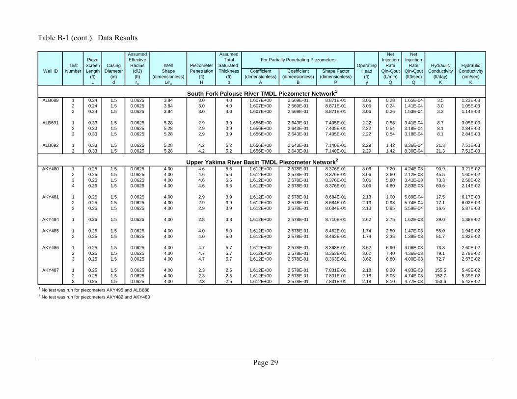
Table B-1 (cont.). Data Results

Assumed Assumed Net NetPiezo Effective Total Injection Injection

Test Screen Casing Radius Well Piezometer Saturated Operating Rate Rate Hydraulic HydraulicWell ID Number Length Diameter (d/2) Shape Penetration Thickness Coefficient Coefficient Shape Factor Head Qin-Qout Qin-Qout Conductivity Conductivity

(ft) (in) (ft) (dimensionless) (ft) (ft) (dimensionless) (dimensionless) (dimensionless) (ft) (L/min) (ft3/sec) (ft/day) (cm/sec)L d rw L/rw H b A B P y Q Q K K

ALB689 1 0.24 1.5 0.0625 3.84 3.0 4.0 1.607E+00 2.569E-01 8.871E-01 3.06 0.28 1.65E-04 3.5 1.23E-032 0.24 1.5 0.0625 3.84 3.0 4.0 1.607E+00 2.569E-01 8.871E-01 3.06 0.24 1.41E-04 3.0 1.05E-033 0.24 1.5 0.0625 3.84 3.0 4.0 1.607E+00 2.569E-01 8.871E-01 3.06 0.26 1.53E-04 3.2 1.14E-03

ALB691 1 0.33 1.5 0.0625 5.28 2.9 3.9 1.656E+00 2.643E-01 7.405E-01 2.22 0.58 3.41E-04 8.7 3.05E-032 0.33 1.5 0.0625 5.28 2.9 3.9 1.656E+00 2.643E-01 7.405E-01 2.22 0.54 3.18E-04 8.1 2.84E-033 0.33 1.5 0.0625 5.28 2.9 3.9 1.656E+00 2.643E-01 7.405E-01 2.22 0.54 3.18E-04 8.1 2.84E-03

ALB692 1 0.33 1.5 0.0625 5.28 4.2 5.2 1.656E+00 2.643E-01 7.140E-01 2.29 1.42 8.36E-04 21.3 7.51E-032 0.33 1.5 0.0625 5.28 4.2 5.2 1.656E+00 2.643E-01 7.140E-01 2.29 1.42 8.36E-04 21.3 7.51E-03



AKY484 1 0.25 1.5 0.0625 4.00 2.8 3.8 1.612E+00 2.578E-01 8.710E-01 2.62 2.75 1.62E-03 39.0 1.38E-02

AKY485 1 0.25 1.5 0.0625 4.00 4.0 5.0 1.612E+00 2.578E-01 8.462E-01 1.74 2.50 1.47E-03 55.0 1.94E-022 0.25 1.5 0.0625 4.00 4.0 5.0 1.612E+00 2.578E-01 8.462E-01 1.74 2.35 1.38E-03 51.7 1.82E-02



1 No test was run for piezometers AKY495 and ALB6882 No test was run for piezometers AKY482 and AKY483

Upper Yakima River Basin TMDL Piezometer Network2

For Partially Penetrating Piezometers

South Fork Palouse River TMDL Piezometer Network1

Table B-2. Sensitivity Analysis Summary

Assumed Assumed Net % Change % ChangePiezo Effective Total Injection of Sensitivity Of K

Parameter Screen Radius Piezometer Saturated Operating Rate Hydraulic Parameter EstimateTest Number Adjustment Length (d/2) Penetration Thickness Head Qin-Qout Conductivity from from

(ft) (ft) (ft) (ft) (ft) (L/min) (ft/day) Base BaseL rw H b y Q K Case Case

se Case AKY486 - Test 1 0.25 0.0625 4.7 5.7 3.62 6.9 73.8

SenTest 1 -1.0 L/min error 5.9 63.1 -14 -14SenTest 2 -0.5 L/min error 6.4 68.4 -7 -7Base Case 6.9 L/min 6.9 73.8 0 0SenTest 3 +0.5 L/min error 7.4 79.1 7 7SenTest 4 +1.0 L/min error 7.9 84.5 14 14

SenTest 5 -0.1 ft error 3.52 75.9 -3 2.8SenTest 6 -0.05 ft error 3.57 74.8 -1 1Base Case 3.62 ft 3.62 73.8 0 0SenTest 7 +0.05 ft error 3.67 72.8 1 -1SenTest 8 +0.1 ft error 3.72 71.8 3 -2.7

SenTest 9 -0.1 ft error 0.15 86.3 -40 17.0SenTest 10 -0.05 ft error 0.2 79.6 -20 8Base Case 0.25 ft 0.25 73.8 0 0SenTest 11 +0.05 ft error 0.3 68.8 20 -7SenTest 12 +0.1 ft error 0.35 64.4 40 -12.7

SenTest 13 -1.0 ft error 3.7 72.5 -21 -1.8SenTest 14 -0.5 ft error 4.2 73.2 -11 -0.8Base Case 4.7 ft 4.7 73.8 0 0.0SenTest 15 +0.5 ft error 5.2 74.3 11 0.7SenTest 16 +1.0 ft error 5.7 74.8 21 1.3

SenTest 17 Fully Penetrating

Ba

1 4.7 125.3 -18 70Base Case Aq. Base 1 ft below piezo 5.7 73.8 0 0SenTest 18 Aq. Base 2 ft below piezo 6.7 70.0 18 -5SenTest 19 Aq. Base 3 ft below piezo 7.7 68.0 35 -8SenTest 20 Aq. Base 10 ft below piezo 14.7 62.7 158 -15SenTest 21 Aq. Base 25 ft below piezo 29.7 59.1 421 -20

Base Case 1.0X casing radius 0.0625 73.8 0 0SenTest 22 1.5X casing radius 0.09375 56.6 50 -23SenTest 23 2.0X casing radius 0.125 46.3 100 -37SenTest 24 3.0X casing radius 0.1875 34.5 200 -53SenTest 25 4.0X casing radius 0.25 27.8 300 -62SenTest 26 5.0X casing radius 0.3125 23.4 400 -68

ther input parameters kept constant*All o1 K estimate calculated using Equations (4) and (7)

Sensitivity Parameter - Screen Length*

Sensitivity Parameter - Operating Head*

Sensitivity Parameter - Injection Rate*

Sensitivity Parameter - Effective Radius*

Sensitivity Parameter - Aquifer Penetration*

Sensitivity Parameter - Piezometer Depth*

Appendix C. EAP Field Data Sheet for Constant Head Injection Test (CHIT)

an evaluation of a piezometer-based constant head

Documents