an empirical model of large-batch training · józefowicz, jakub pachocki, michael petrov, henrique...
TRANSCRIPT

An Empirical Model of Large-Batch Training
Sam McCandlish∗OpenAI
Jared KaplanJohns Hopkins University, OpenAI
Dario AmodeiOpenAI
and the OpenAI Dota Team†
Abstract
In an increasing number of domains it has been demonstrated that deep learning models canbe trained using relatively large batch sizes without sacrificing data efficiency. However thelimits of this massive data parallelism seem to differ from domain to domain, ranging frombatches of tens of thousands in ImageNet to batches of millions in RL agents that playthe game Dota 2. To our knowledge there is limited conceptual understanding of whythese limits to batch size differ or how we might choose the correct batch size in a newdomain. In this paper, we demonstrate that a simple and easy-to-measure statistic calledthe gradient noise scale predicts the largest useful batch size across many domains andapplications, including a number of supervised learning datasets (MNIST, SVHN, CIFAR-10, ImageNet, Billion Word), reinforcement learning domains (Atari and Dota), and evengenerative model training (autoencoders on SVHN). We find that the noise scale increasesas the loss decreases over a training run and depends on the model size primarily throughimproved model performance. Our empirically-motivated theory also describes the tradeoffbetween compute-efficiency and time-efficiency, and provides a rough model of the benefitsof adaptive batch-size training.
∗Work done as an OpenAI Fellow.†The OpenAI Dota Team (Greg Brockman, Brooke Chan, Przemysław Debiak, Christy Dennison, David Farhi, Rafał
Józefowicz, Jakub Pachocki, Michael Petrov, Henrique Pondé, Jonathan Raiman, Szymon Sidor, Jie Tang, Filip Wolski,and Susan Zhang) performed measurements of the reinforcement learning agents they developed for the game Dota 2.The Dota team’s work can be cited as [BCD+18].

Contents
1 Introduction 2
2 Theory and Predictions for the Gradient Noise Scale 4
3 Experiments 9
4 Related Work 14
5 Discussion 15
A Methods 17
B Results for All Tasks 19
C Temperature and the Noise Scale 25
D Dynamically Varying the Batch Size 26
E Comments on Optimization 29
1 Introduction
The last few years have seen a rapid increase in the amount of computation used to train deep learning models[AH18]. A major enabler as well as a limiting factor in this growth has been parallelism – the extent to whicha training process can be usefully spread across multiple devices. Regardless of how much total computationis available, if model training cannot be sufficiently parallelized, then it may take too much serial time andtherefore may be practically infeasible.
A very common source of parallelism in deep learning has been data parallelism, which involves splittinga batch of data across multiple devices and then aggregating and applying the resulting gradients. Dataparallelism requires fast communication between devices, but also requires that large batches are algorithmi-cally effective in accelerating learning. Recently, a number of papers have shown empirically that on spe-cific datasets or tasks, large batch sizes can achieve almost linear speed-ups in training without substantiallyharming sample efficiency or generalization. For example, batch sizes of 8 thousand [GDG+17], 16 thousand[SKYL17], 32 thousand [YGG17, YZH+17, ASF17], and even 64 thousand [JSH+18] examples have beeneffectively employed to train ImageNet, and batch sizes of thousands have been effective for language mod-els and generative models [OEGA18, PKYC18, BDS18]. This phenomenon is not confined to supervisedlearning: in reinforcement learning, batch sizes of over a million timesteps (with tens of thousands of envi-ronments running in parallel) have been used in a Dota-playing agent [BCD+18], and even in simple Atarienvironments batch sizes of several thousand timesteps have proved effective [AAG+18, HQB+18, SA18].These discoveries have allowed massive amounts of data and computation to be productively poured intomodels in a reasonable amount of time, enabling more powerful models in supervised learning, RL, and otherdomains.
However, for a given dataset and model, there is little to guide us in predicting how large a batch size wecan feasibly use, why that number takes a particular value, or how we would expect it to differ if we useda different dataset or model. For example, why can we apparently use a batch size of over a million whentraining a Dota agent, but only thousands or tens of thousands when training an image recognition model? Inpractice researchers tend to simply experiment with batch sizes and see what works, but a downside of thisis that large batch sizes often require careful tuning to be effective (for example, they may require a warmup
2

Figure 1: The tradeoff between time and compute resources spent to train a model to a given level of perfor-mance takes the form of a Pareto frontier (left). Training time and compute cost are primarily determined bythe number of optimization steps and the number of training examples processed, respectively. We can traina model more quickly at the cost of using more compute resources. On the right we show a concrete exampleof the Pareto frontiers obtained from training a model to solve the Atari Breakout game to different levels ofperformance. The cost and training time depend on the computing architecture and are shown approximately.
period or an unusual learning rate schedule), so the fact that it is possible to use a large batch size canremain undiscovered for a long time. For example, both the Atari and ImageNet tasks were for several yearsconventionally run with a substantially smaller batch size than is now understood to be possible. Knowingahead of time what batch size we expect to be effective would be a significant practical advantage in trainingnew models.
In this paper we attempt to answer some of these questions. We measure a simple empirical statistic, thegradient noise scale3 (essentially a measure of the signal-to-noise ratio of gradient across training examples),and show that it can approximately predict the largest efficient batch size for a wide range of tasks. Our modelalso predicts a specific shape for the compute/time tradeoff curve, illustrated in Figure 1. Our contributionsare a mix of fairly elementary theory and extensive empirical testing of that theory.
On the conceptual side, we derive a framework which predicts, under some basic assumptions, that trainingshould parallelize almost linearly up to a batch size equal to the noise scale, after which there should be asmooth but relatively rapid switch to a regime where further parallelism provides minimal benefits. Addition-ally, we expect that the noise scale should increase during training as models get more accurate, and shouldbe larger for more complex tasks, but should not have a strong dependence on model size per se. We alsoprovide an analysis of the efficiency gains to be expected from dynamically adjusting the batch size accordingto noise scale during training. Finally, we predict that, all else equal, the noise scale will tend to be larger incomplex RL tasks due to the stochasticity of the environment and the additional variance introduced by thecredit assignment problem.
On the empirical side, we verify these predictions across 8 tasks in supervised learning, RL, and gener-ative models, including ImageNet, CIFAR-10, SVHN, MNIST, BillionWord, Atari, OpenAI’s Dota agent[BCD+18], and a variational autoencoder for images. For each of these tasks we demonstrate that the noisescale accurately predicts the largest usable batch size (at the order of magnitude level) and that gains to paral-lelism degrade in the manner predicted by theory. We also show that the noise scale increases over the courseof training and demonstrate efficiency gains from dynamic batch size tuning. The noise scale eventuallybecomes larger for more performant models, but this appears to be caused by the fact that more performantmodels simply achieve a better loss.
The rest of this paper is organized as follows. In Section 2, we derive a simple conceptual picture of thenoise scale, data parallelism, and batch sizes, and explain what it predicts about optimal batch sizes and how
3Similar metrics have appeared previously in the literature. We discuss related work in Section 4.
3

Figure 2: Less noisy gradient estimates allow SGD-type optimizers to take larger steps, leading to conver-gence in a smaller number of iterations. As an illustration, we show two optimization trajectories usingmomentum in a quadratic loss, with different step sizes and different amounts of artificial noise added to thegradient.
they vary over the course of training and across tasks. We build on this analysis to study training efficiency inSection 2.3. Then in Section 3 we empirically test the predictions in Section 2 and explore how the noise scalevaries with dataset, model size, and learning paradigm (supervised learning vs RL vs generative models).Section 4 describes related work and Section 5 discusses the implications of these results and possible futureexperiments.
2 Theory and Predictions for the Gradient Noise Scale
2.1 Intuitive Picture
Before working through the details of the gradient noise scale and the batch size, it is useful to present theintuitive picture. Suppose we have a function we wish to optimize via stochastic gradient descent (SGD).There is some underlying true optimization landscape, corresponding to the loss over the entire dataset (or,more abstractly, the loss over the distribution it is drawn from). When we perform an SGD update with afinite batch size, we’re approximating the gradient to this true loss. How should we decide what batch size touse?
When the batch size is very small, the approximation will have very high variance, and the resulting gradientupdate will be mostly noise. Applying a bunch of these SGD updates successively will average out thevariance and push us overall in the right direction, but the individual updates to the parameters won’t be veryhelpful, and we could have done almost as well by aggregating these updates in parallel and applying themall at once (in other words, by using a larger batch size). For an illustrative comparison between large andsmall batch training, see Figure 2.
By contrast, when the batch size is very large, the batch gradient will almost exactly match the true gradient,and correspondingly two randomly sampled batches will have almost the same gradient. As a result, doublingthe batch size will barely improve the update – we will use twice as much computation for little gain.
Intuitively, the transition between the first regime (where increasing the batch size leads to almost perfectlylinear speedups) and the second regime (where increasing the batch size mostly wastes computation) shouldoccur roughly where the noise and signal of the gradient are balanced – where the variance of the gradient isat the same scale as the gradient itself4. Formalizing this heuristic observation leads to the noise scale.
The situation is shown pictorially in Figure 1. For a given model, we’d like to train it in as little wall timeas possible (x-axis) while also using as little total computation as possible (y-axis) – this is the usual goal
4Note that these considerations are completely agnostic about the size of the dataset itself.
4

of parallelization. Changing the batch size moves us along a tradeoff curve between the two. Initially, wecan increase the batch size without much increase in total computation, then there is a “turning point” wherethere is a substantive tradeoff between the two, and finally when the batch size is large we cannot make furthergains in training time. In the conceptual and experimental results below, we formalize these concepts andshow that the bend in the curve (and thus the approximate largest effective batch size) is in fact set roughlyby the noise scale.
2.2 Gradients, Batches, and the Gradient Noise Scale
We’ll now formalize the intuitions described in Section 2.1. Consider a model, parameterized by variablesθ ∈ RD, whose performance is assessed by a loss function L (θ). The loss function is given by an averageover a distribution ρ (x) over data points x. Each data point x has an associated loss function Lx (θ), and thefull loss is given by L (θ) = Ex∼ρ [Lx (θ)]5.
We would like to minimizeL (θ) using an SGD-like optimizer, so the relevant quantity is the gradientG (θ) =∇L (θ). However, optimizing L (θ) directly would be wasteful if not impossible, since it would requireprocessing the entire data distribution every optimization step. Instead, we obtain an estimate of the gradientby averaging over a collection of samples from ρ, called a batch:
Gest (θ) =1
B
B∑i=1
∇θLxi(θ) ; xi ∼ ρ (2.1)
This approximation forms the basis for stochastic optimization methods such as mini-batch stochastic gradi-ent descent (SGD) and Adam [KB14]. The gradient is now a random variable whose expected value (averagedover random batches) is given by the true gradient. Its variance scales inversely with the batch size B6:
Ex1···B∼ρ [Gest (θ)] = G (θ)
covx1···B∼ρ (Gest (θ)) =1
BΣ (θ) , (2.2)
where the per-example covariance matrix is defined by
Σ (θ) ≡ covx∼ρ (∇θLx (θ))
= Ex∼ρ[(∇θLx (θ)) (∇θLx (θ))
T]−G (θ)G (θ)
T. (2.3)
The key point here is that the minibatch gradient gives a noisy estimate of the true gradient, and that largerbatches give higher quality estimates. We are interested in how useful the gradient is for optimization pur-poses as a function of B, and how that might guide us in choosing a good B. We can do this by connectingthe noise in the gradient to the maximum improvement in true loss that we can expect from a single gradientupdate. To start, let G denote the true gradient and H the true Hessian at parameter values θ. If we perturbthe parameters θ by some vector V to θ − εV , where ε is the step size, we can expand true loss at this newpoint to quadratic order in ε:
L (θ − εV ) ≈ L (θ)− εGTV +1
2ε2V THV. (2.4)
If we had access to the noiseless true gradient G and used it to perturb the parameters, then Equation 2.4 withV = G would be minimized by setting ε = εmax ≡ |G|2
GTHG. However, in reality we have access only to the
noisy estimated gradient Gest from a batch of size B, thus the best we can do is minimize the expectation
5In the context of reinforcement learning, the loss could be the surrogate policy gradient loss, and the distribution ρwould be nonstationary.
6This is strictly true only when training examples are sampled independently from the same data distribution. For ex-ample, when batches are sampled without replacement from a dataset of sizeD, the variance instead scales like
(1B− 1
D
).
For simplicity, we restrict ourself to the case where B � D or where batches are sampled with replacement, but ourconclusions can be altered straightforwardly to account for correlated samples.
5
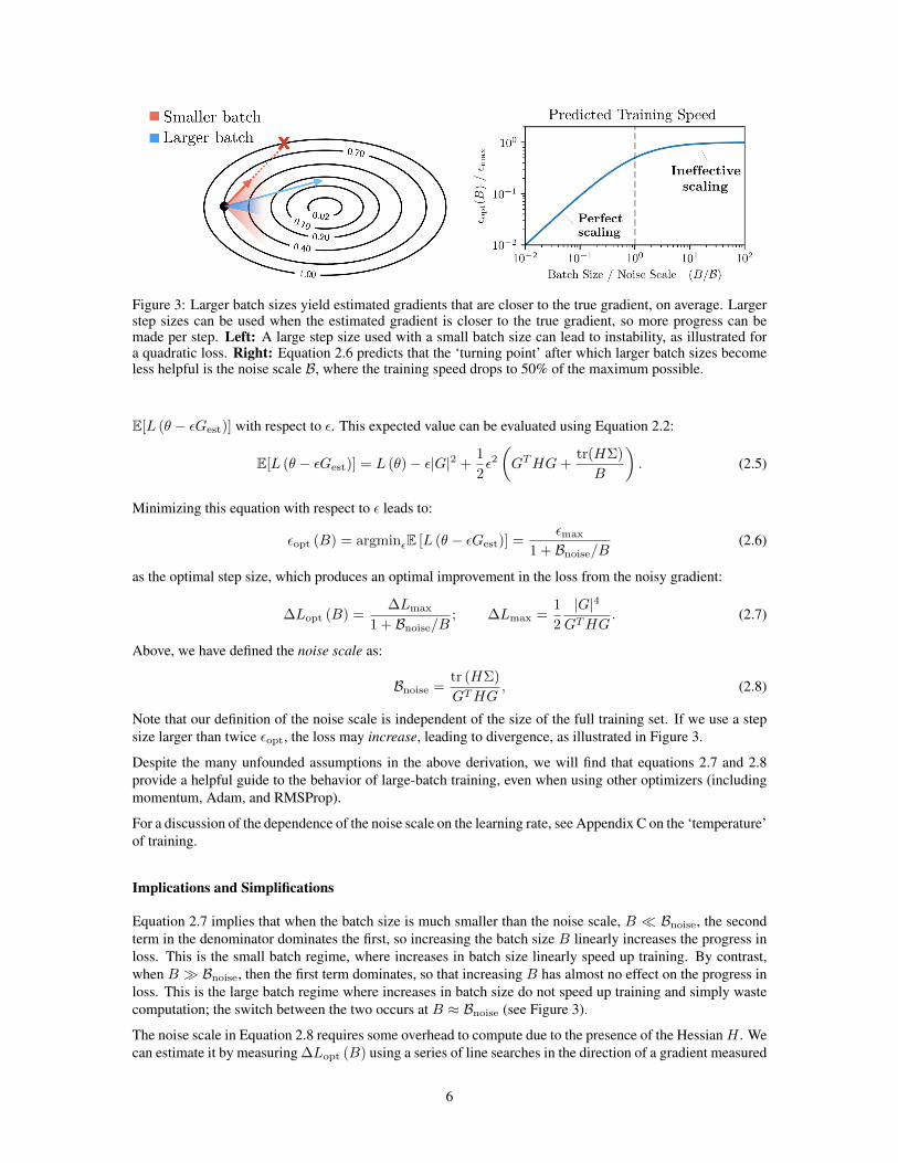
Figure 3: Larger batch sizes yield estimated gradients that are closer to the true gradient, on average. Largerstep sizes can be used when the estimated gradient is closer to the true gradient, so more progress can bemade per step. Left: A large step size used with a small batch size can lead to instability, as illustrated fora quadratic loss. Right: Equation 2.6 predicts that the ‘turning point’ after which larger batch sizes becomeless helpful is the noise scale B, where the training speed drops to 50% of the maximum possible.
E[L (θ − εGest)] with respect to ε. This expected value can be evaluated using Equation 2.2:
E[L (θ − εGest)] = L (θ)− ε|G|2 +1
2ε2(GTHG+
tr(HΣ)
B
). (2.5)
Minimizing this equation with respect to ε leads to:
εopt (B) = argminεE [L (θ − εGest)] =εmax
1 + Bnoise/B(2.6)
as the optimal step size, which produces an optimal improvement in the loss from the noisy gradient:
∆Lopt (B) =∆Lmax
1 + Bnoise/B; ∆Lmax =
1
2
|G|4
GTHG. (2.7)
Above, we have defined the noise scale as:
Bnoise =tr (HΣ)
GTHG, (2.8)
Note that our definition of the noise scale is independent of the size of the full training set. If we use a stepsize larger than twice εopt, the loss may increase, leading to divergence, as illustrated in Figure 3.
Despite the many unfounded assumptions in the above derivation, we will find that equations 2.7 and 2.8provide a helpful guide to the behavior of large-batch training, even when using other optimizers (includingmomentum, Adam, and RMSProp).
For a discussion of the dependence of the noise scale on the learning rate, see Appendix C on the ‘temperature’of training.
Implications and Simplifications
Equation 2.7 implies that when the batch size is much smaller than the noise scale, B � Bnoise, the secondterm in the denominator dominates the first, so increasing the batch size B linearly increases the progress inloss. This is the small batch regime, where increases in batch size linearly speed up training. By contrast,when B � Bnoise, then the first term dominates, so that increasing B has almost no effect on the progress inloss. This is the large batch regime where increases in batch size do not speed up training and simply wastecomputation; the switch between the two occurs at B ≈ Bnoise (see Figure 3).
The noise scale in Equation 2.8 requires some overhead to compute due to the presence of the HessianH . Wecan estimate it by measuring ∆Lopt (B) using a series of line searches in the direction of a gradient measured
6

with various batch sizes B and fitting the result to Equation 2.7. This allows us to estimate Bnoise as well asto empirically test whether Equation 2.7 actually fits the data (we discuss these local tests more in Section 3).
The situation gets even simpler if we make the (unrealistic) assumption that the optimization is perfectlywell-conditioned – that the Hessian is a multiple of the identity matrix. If that is the case, then Equation 2.8reduces to:
Bsimple =tr(Σ)
|G|2, (2.9)
which says that the noise scale is equal to the sum of the variances of the individual gradient components,divided by the global norm of the gradient7 – essentially a measure of how large the gradient is compared toits variance. It is also a measure of the scale at which the estimated and true gradient become close in L2
space (having non-trivial dot product) – the expected normalized L2 distance is given by:
E[|Gest −G|2
]|G|2
=1
B
tr(Σ)
|G|2=Bsimple
B, (2.10)
In practice, we find that Bsimple and Bnoise typically differ only by a small constant multiplicative factor,particularly when we employ common training schemes that improve conditioning. In our empirical work wewill sometimes compute Bnoise, but will primarily compute Bsimple instead, as it requires less computationalexpense. In Appendix A.1, we provide an extremely simple method to measure this simplified noise scalewith negligible overhead in the context of data-parallel training.
2.3 Predictions for Data/Time Efficiency Tradeoffs
Thus far our analysis has only involved a single point in the loss landscape. But in Section 3 we will showthat Equation 2.7 nevertheless predicts the dependence of training speed on batch size remarkably well, evenfor full training runs that range over many points in the loss landscape. By averaging Equation 2.7 overmultiple optimization steps (see Appendix D), we find a simple relationship between training speed and dataefficiency:
S
Smin− 1 =
(E
Emin− 1
)−1. (2.11)
Here, S and Smin represent the actual and minimum possible number of steps taken to reach a specified levelof performance, respectively, and E and Emin represent the actual and minimum possible number of trainingexamples processed to reach that same level of performance. Since we are training at fixed batch size8, wehave Etot = BStot. We define the critical batch size by an empirical fit to the above equation, as
Bcrit =Emin
Smin. (2.12)
Our model predicts Bcrit ≈ Bnoise, where Bnoise is appropriately averaged over training (see Appendix D).Note that the noise scale can vary significantly over the course of a training run, so the critical batch size alsodepends on the level of performance to which we train the model.
The resulting tradeoff curve in serial time vs total compute has a hyperbolic shape represented in Figure 1.The goal of optimization is to reach a given level of performance with minimal S and E – but as depictedin Figure 1, there are tradeoffs involved, as very small S may require very large E, and vice versa. Whenwe choose B = Bcrit, the two sides of Equation 2.11 are both 1, so that training takes twice as many passesthrough the training data as an optimally data-efficient (small-batch) run would take, and twice as manyoptimization steps as an optimally time-efficient (large-batch) run would take.
7One might also use preconditioned gradients, obtained for example by dividing gradient components by the squareroot of the Adam optimizer’s [KB14] accumulated variances. We experimented with this but found mixed results.
8We discuss the benefits of dynamically varying the batch size in Appendix D
7

2.4 Assumptions and Caveats
The mathematical argument in the previous sections depends on several assumptions and caveats, and it isuseful to list these all in one place, in order to help clarify where and why we might expect the quantities inequations 2.8 and 2.9 to be relevant to training:
1. Short-horizon bias: The picture in Section 2.2 is a strictly local picture – it tells us how to bestimprove the loss on the next gradient step. Greedily choosing the best local improvement is gen-erally not the best way to globally optimize the loss (see e.g. [WRLG18]). For example, greedyoptimization might perform poorly in the presence of bad local minima or when the landscape is ill-conditioned. The critical batch size would then be reduced by the extent to which noise is beneficial.
2. Poor conditioning: In poorly conditioned optimization problems, parameter values often oscillatealong the large-curvature directions rather than decreasing in a predictable way (see e.g. [Goh17] andAppendix E.1). This means that Equation 2.7 will not perfectly reflect the amount of optimizationprogress made per step. Nevertheless, we will see that it still accurately predicts the relative speedof training at different batch sizes via the resulting tradeoff Equation 2.11.
3. Simplified noise scale: As noted in Section 2.2, whenever we use the simplified noise scale (Equa-tion 2.9) rather than the exact noise scale (Equation 2.8), this number may be inaccurate to theextent that the Hessian is not well-conditioned. Different components of the gradient can have verydifferent noise scales.
4. Learning rate tuning: The arguments in Section 2.2 assume that we take the optimal step size andmaximize the expected improvement in loss, Equation 2.6. In practice learning rates are unlikelyto be perfectly tuned, so that the actual improvement in loss (and thus the scaling of training withbatch size) may not perfectly reflect Equation 2.7. However, by trying to choose the best learningrate schedules (or by simply doing a grid search) we can reduce this source of error. In addition, thenoise scale depends strongly on the learning rate via a ‘temperature’ of training, though this sourceof error is small as long as the learning rate is reasonably close to optimal. We provide a moredetailed discussion of this dependence in Appendix C.
5. Quadratic approximation: The Taylor expansion in Equation 2.4 is only to second order, so ifthird order terms are important, in either the distribution of gradient samples or the optimizationlandscape, then this may introduce deviations from our conceptual model, and in particular devi-ations from Equation 2.7. Intuitively, since parameter updates are local and often quite small wesuspect that the previous two sources of error will be more important than this third one.
6. Generalization: The picture in Section 2.2 says nothing about generalization – it is strictly aboutoptimizing the training loss as a mathematical function. Some papers have reported a “generaliza-tion gap” in which large batch sizes lead to good training loss but cause a degradation in test loss,apparently unrelated to overfitting [KMN+16, HHS17]. The arguments in Section 2.2 don’t excludethis possibility, but recent work [SLA+18] has found no evidence of a generalization gap whenhyperparameters are properly tuned.
Despite these potential issues in our conceptual model, we’ll show in Section 3 that the noise scale is overalla good empirical predictor of the critical batch size. Furthermore, we will see that most training runs fitEquation 2.11 remarkably well.
2.5 Expected Patterns in the Noise Scale
In the next section we will measure the noise scale for a number of datasets and confirm its properties.However, it is worth laying out a few patterns we would expect it to exhibit on general grounds:
• Larger for difficult tasks: We expect B to be larger for more complex/difficult9 tasks, becauseindividual data points will be less correlated, or only correlated in a more abstract way. This may
9To be clear, we do not expect this to be the primary difference between more and less difficult tasks. Other difficultymetrics such as the intrinsic dimensionality [LFLY18] appear to be unrelated to the amount of gradient noise, though itwould be interesting if there were some connection.
8

apply both over the course of training on a given dataset (where we may pick the ‘low-hanging fruit’first, leaving a long tail of more complicated things to learn) or in moving from easier to harderdatasets and environments. In reinforcement learning, we expect environments with sparse rewardsor long time horizons to have larger noise scale. We also expect generative models to have smallerB as compared to classifiers training on the same dataset, as generative models may obtain moreinformation from each example.
• Growth over training: B will grow when the gradient decreases in magnitude, as long as the noisetr(Σ) stays roughly constant. Since |G| decreases as we approach the minimum of a smooth loss,we would expect B to increase during neural network training.
• Weak dependence on model size: The number of model parameters in the neural network cancelsin the noise scale, so we do not expect B to exhibit a strong dependence on model size (at fixedloss). As discussed above, models that achieve better loss will tend to have a higher noise scale,and larger models often achieve better loss, so in practice we do expect larger models to have highernoise scale, but only through the mechanism of achieving better loss.
• Learning rate tuning: The noise scale will be artificially inflated if the learning rate is too small,due to the ‘temperature’ dependence described in Appendix C. To get a useful measurement of thenoise scale, the learning rate needs to be appropriate to the current point in parameter space.
The first and last points can be exhibited analytically in toy models (see Appendix C), but we do not expecttheoretical analyses to provide a great deal of insight beyond the intuitions above. Instead, we will focus onconfirming these expectations empirically.
2.6 Summary
To summarize, our model makes the following predictions about large-batch training:
• The tradeoff between the speed and efficiency of neural network training is controlled by the batchsize and follows the form of Equation 2.11.
• The critical batch size Bcrit characterizing cost/time tradeoffs can be predicted at the order of mag-nitude level by measuring the gradient noise scale, most easily in the simplified form Bsimple fromEquation 2.9.
• The noise scale can vary significantly over the course of a training run, which suggests that thecritical batch size also depends on the chosen level of model performance.
• The noise scale depends on the learning rate via the ‘temperature’ of training, but is consistentbetween well-tuned training runs (see Appendix C).
3 Experiments
We now test the predictions of Section 2 on a range of tasks, including image classification, language mod-eling, reinforcement learning, and generative modeling. The tasks range from very simple (MNIST) to verycomplex (5v5 Dota), which allows us to test our model’s predictions in drastically varying circumstances.Our central experimental test is to compare the prediction made by the gradient noise scale Bsimple for eachtask, to the actual limits of batch size Bcrit found by carefully tuned full training runs at an exhaustive rangeof batch sizes. The overall results of this comparison are summarized in Figure 4. We find that the gradientnoise scale predicts the critical batch size at the order of magnitude level, even as the latter varies from 20(for an SVHN autoencoder) to over 10 million (consistent with prior results reported in [BCD+18]). Detailsabout the hyperparameters, network architectures, and batch size searches are described in Appendix A.4.Below we describe the individual tasks, the detailed measurements we perform on each task, and the resultsof these measurements.
9

Figure 4: The “simple noise scale” roughly predicts the maximum useful batch size for many ML tasks.We define this “critical batch size” to be the point at which compute efficiency drops below 50% optimal, atwhich point training speed is also typically 50% of optimal. Batch sizes reported in number of images, tokens(for language models), or observations (for games). We show the critical batch size for a full training run,and the noise scale appropriately averaged over a training run (see Appendix D). Due to resource constraints,for Dota 5v5 we show the batch size used by the OpenAI Dota team as a lower bound for the critical batchsize.
Figure 5: Left: The optimal learning rate is displayed for a range of batch sizes, for an SVHN classifiertrained with SGD. The optimal learning rate initially scales linearly as we increase the batch size, leveling offin the way predicted by Equation 2.7. Right: For a range of batch sizes, we display the average loss progress∆L (B) that can be made from a batch of size B via a line search, normalized by the measured ∆L (Bmax).Early in training, smaller batches are sufficient to make optimal progress, while larger batches are requiredlater in training.
3.1 Quantities Measured
In order to test our model we train each task on a range of batch sizes, selecting the optimal constant learningrate separately for each batch size using a simple grid search. Across a range of tasks, we produce thefollowing results and compare with our model:
• Optimal learning rates: When optimizing with plain SGD or momentum, we find that the optimallearning rate follows the functional form of Equation 2.6, as shown in Figure 5. For Adam andRMSProp the optimal learning rate initially obeys a power law ε (B) ∝ Bα with α between 0.5 and1.0 depending on the task, then becomes roughly constant. The scale at which the optimal learning
10

Figure 6: Training runs for a simple CNN classifier on the SVHN dataset at constant batch sizes. Small batchtraining is more compute-efficient (right), while large-batch training requires fewer optimizer steps (left). Theturning point between time-efficient and compute-efficient training occurs roughly at B = 64 for the initialphase of training and increases later in training.
rate stops increasing is generally somewhat smaller than the typical noise scale. (See Appendix E.2for a potential explanation for this power law behavior.)
• Pareto frontiers: For each batch size, we observe the number of optimization steps and total numberof data samples needed to achieve various levels of performance. This allows us to visualize thetradeoff between time-efficiency and compute-efficiency as a Pareto frontier (see Figures 6 and 7).We find that Equation 2.11 fits the shape of these tradeoff curves remarkably well in most cases.
• Critical batch size (Bcrit): We determine the critical batch size over the course of a training runby fitting the Pareto fronts to the functional form of Equation 2.11 (see Figure 7). This quantifiesthe point at which scaling efficiency begins to drop. In particular, training runs at batch sizes muchless than Bcrit behave similarly per training example, while training runs at batch sizes much largerthan Bcrit behave similarly per optimization step (see Figure 6). The critical batch size typicallyincreases by an order of magnitude or more over the course of training.
• Simple noise scale (Bsimple): We measure the simple noise scale of Equation 2.9 over the course ofa single training run using the minimal-overhead procedure described in Appendix A.1. Note thatsome care must be taken to obtain a proper estimate of Bsimple due to its dependence on the learningrate via the ‘temperature’ of training. We find that the noise scale agrees between different well-tuned training runs when compared at equal values of the loss, so it can be accurately measured atsmall batch size (see Appendix C). We also find that, aside from some fluctuations early in training,Bsimple typically predicts the critical batch size at the order of magnitude level (see Figure 7). Thenoise scale also typically increases over the course of training, tracking the critical batch size. Toobtain a single value for the noise scale representing a full training run, we average over a trainingrun as described in Appendix D.
• Full noise scale (Bnoise): For SVHN trained with SGD, we also measure the full noise scale Bnoiseby performing line searches for gradients obtained by batches of varying size, then fit to the func-tional form 2.11 (see Figures 5 and 7). This is a somewhat better estimate of Bcrit but is lesscomputationally convenient, so we choose to focus on Bsimple for the remaining tasks.
3.2 Results
We summarize our findings in Figure 4: across many tasks, the typical simple noise scale approximatelypredicts the batch size at which the returns from increasing scale begin to diminish significantly. Results forall of the tasks can be found in Appendix B. We provide a detailed discussion of our methods in Appendix A.
11

Figure 7: The tradeoff between time-efficiency and compute-efficiency can be visualized as a Pareto frontier.Each point on the diagram above (left) represents the number of optimizer steps and processed examplesneeded to achieve a particular level of classification accuracy. Fits to Equation 2.11 are also shown.
Supervised Learning
Basic image classification results are pictured in Figure 14.
• SVHN We train a simple CNN image classifier on the extended SVHN dataset [NWC+11]. Wedisplay all three of Bcrit, Bsimple, and Bnoise for SVHN optimized with SGD in Figure 7. We findthat Bnoise better-predicts Bcrit as compared to the more naive Bsimple. We compare to trainingusing the Adam optimizer [KB14] in Figure 14, where Bsimple provides a very accurate predictionfor Bcrit.
• MNIST We train a simple CNN on the MNIST dataset [LC10] using SGD, and find that Bsimple
roughly estimates Bcrit, though the latter is significantly smaller.
• CIFAR10 We train a size 32 ResNet [HZRS15] with Momentum on CIFAR10 [Kri09] and find thatBsimple predicts Bcrit.
• ImageNet We train a size 50 ResNet [HZRS15] with Momentum on ImageNet [DDS+09], and use alearning rate schedule that decays the learning rate three times during training. Due to the schedule,both Bsimple, and Bcrit change significantly during training (see Appendix C for a discussion) andmust be measured separately at each learning rate. Results are pictured in Figure 10. We find thatthe noise scale varies from 2,000 to 100,000 in the main phase of training, which matches empiricalwork (e.g. [JSH+18]) showing that constant batch sizes up to 64 thousand can be used without aloss of efficiency. During the later fine-tuning phase of training, the noise scale increases further tohundreds of thousands and even millions, suggesting that even larger batch sizes may be useful atthe very end of training. Our critical batch sizes are slightly lower (15k vs 64k) than those reportedin the literature, but we did not use the latest techniques such as layer-wise adaptive learning rates[YGG17].
Overall we find that more complex image datasets have larger noise scales in a way that is not directlydetermined by dataset size.
Generative Modeling
The results for these tasks are pictured in Figure 9.
• VAE and Autoencoder We train a VAE [KW13] and a simple Autoencoder on the SVHN dataset[NWC+11]; we were motivated to compare these models because VAEs introduce additionalstochasticity. As expected, the VAE had larger Bcrit and Bsimple as compared to the Autoencoder,and both models had much lower Bsimple as compared to SVHN image classifiers. However, unlikemost of the other tasks, for these generative models Bsimple was significantly smaller than Bcrit.
• Language Modeling We train a single-layer LSTM for autoregressive prediction on the BillionWord dataset [CMS+13], and find good agreement between Bcrit and Bsimple. We also illustrate the
12
dependence on LSTM size in Figure 8, finding that the noise scale is roughly independent of LSTMsize at fixed values of the loss, but that larger LSTMs eventually achieve lower values of the loss anda larger noise scale.
Reinforcement Learning
• Atari We train RL agents with the policy gradient algorithm A2C [MBM+16] on seven Atari games[BNVB12] (Alien, Beamrider, Breakout, Pong, Qbert, Seaquest, Space Invaders), with results pic-tured in Figures 11 and 12. The tradeoff curves generally agree well with the prediction of Equation2.11, though they are somewhat noisy e.g. for Pong since we do not average over multiple seeds.For some Atari games, we find some consistent deviation from 12 at very small batch sizes (see e.g.Beam Rider in Figure 11). It would be interesting to study this phenomenon further, though thiscould simply indicate greater sensitivity to other hyperparameters (e.g. momentum) at small batchsize. Overall, we see that patterns in the noise scale match intuition, such as Pong being much easierto learn than other Atari games.
• Dota The OpenAI Dota team has made it possible to train PPO [SWD+17] agents on both Dota 1v1and 5v5 environments (the latter being preliminary ongoing work). We vary the two hyperparametersbatch size and learning rate on the existing code, experiment setup, and training infrastructure asdescribed in [BCD+18]. The Dota 1v1 environment features two agents fighting in a restricted partof the map (although they are free to walk anywhere) with a fixed set of abilities and skills, whereasDota 5v5 involves the whole map, 5 heroes on each side, and vastly more configurations in whichheroes might engage each other. This is reflected in the higher noise scale for Dota 5v5 (at least10 million) relative to Dota 1v1 – we suspect the higher diversity of situations gives rise to morevariance in the gradients. Due to resource constraints we were not able to measure the Pareto frontsfor Dota 5v5, and so we can only report the batch size used by the Dota team and the measured noisescale.
Results for the tasks described above were generally within a reasonable margin of state-of-the-art results,though we did not explicitly try to match SOTA or use special algorithmic or architectural tricks. Our goalwas simply to confirm that we were in a reasonably well-performing regime that is typical of ML practice.
For the supervised learning and generative modeling tasks listed above, we have the option of using eithertraining set or test set performance to compare different batch sizes. For the main results in this paper, wechoose train set performance because it is what is directly predicted by our model, and because it is easier tomeasure in the presence of overfitting. The choice makes negligible difference in most of our experiments,either because they involve RL or because the datasets are large enough that we don’t overfit. On the smalldatasets MNIST, CIFAR10, and SVHN, overfitting makes measurement of test error more difficult, but we domeasure the test error behavior in Appendix E.3, and both the Pareto fronts and critical batch size generallydo not change much.
The fact that the noise scale is consistent between well-tuned training runs suggests that the correspondingoptimization trajectories are similar in some sense. In Appendix C we investigate this idea further and relatethe noise scale to a characteristic ‘temperature’ of the training process.
Model Size Dependence
The definitions of the noise scales do not have any manifest dependence on the number of parameters in amodel. We have conjectured that they will be roughly independent of model size at fixed values of the loss.
LSTM language models provide a natural test case, since LSTM sizes can be scaled up without qualitativelyaltering model architecture. As shown in Figure 8, the simple noise scale appears to be roughly independentof model size at a fixed value of the loss. However, due to their higher performance and lower achieved loss,larger models eventually reach larger noise scales than smaller models. We do not have specific hypothesesfor how the noise scale should vary with model architecture, but interesting results along these lines wererecently obtained [SLA+18].
13

Figure 8: We show the relationship between training perplexity and the simple noise scale (left) for a rangeof LSTM sizes on the Billion Word dataset. These results show that at fixed values of the loss, the noise scaledoes not depend significantly on model size. On the right we show the simple noise scale during training,plotted in terms of the number of tokens processed. After processing a given number of examples, largermodels will tend to have a larger noise scale, but only as a consequence of having achieved smaller loss.
4 Related Work
A great deal of prior work has studied large-batch training, investigated versions of the noise scale, exploredadaptive batch size and learning rate schedules, and demonstrated that large batch training can be effectiveon specific datasets. We attempt to summarize this work below.
Recent papers have probed the limits of large batch training empirically, especially for ImageNet [GDG+17,YZH+17, JSH+18], in some cases using layer-wise adaptive learning-rates [YGG17]. More recent workhas demonstrated that large batch training can also be applied to RL [AAG+18, BCD+18, SA18, HQB+18].The use of second order optimization methods [BGM17] might increase the utility of data parallelism evenfurther. A thorough review of large batch training and potential issues with generalization was provided in avery nice recent empirical study [SLA+18] done in parallel with this work. [GVY+18] also systematicallystudied large-batch training, though it did not tune the learning rate separately for each batch size.
Other recent work has explored the impact of gradient noise on optimization speed and batch size selec-tion. [SZL13] connected gradient noise and the locally optimal step size to identify an adaptive learningrate. [MHB17] derived a sampling distribution for SGD, motivating our definition of ‘temperature’. [SL17]connected this temperature to the critical batch size, though they predict a dependence on dataset size whichwe do not observe. [SZT17] identified a signal-dominated and noise-dominated phase of training. [SKYL17]showed that decaying the learning rate and increasing the batch size have the same effect, motivated by theSGD training temperature. ([DNG17] also suggested increasing learning rate and batch size together, but withdifferent motivation.) [IES+18] empirically investigated the role of gradient noise in reinforcement learning.
The gradient noise scale in particular has also been studied in earlier work to aid in batch size selection.The noise scale itself is used implicitly in basic statistical techniques for sample size selection (see e.g.[Wik, NIS]). [BCNW12] implicitly uses the gradient noise scale for a theoretical analysis of batch sizeselection. [BCN16, DYJG16, BRH16] propose adaptive sampling methods based on the gradient noise scalein the context of neural network optimization. [YPL+17] analyzed the gradient noise scale for a particularclass of functions and related it to the critical batch size, though it predicts a sharp change in learning speedwith batch size rather than the smooth change we observe. [CWZ+18] theoretically analyzed the dependenceof the gradient noise scale on network width for shallow or linear networks, though they find inconsistentempirical results on neural networks. [MBB17] found a formula for the optimization speedup in terms ofbatch size resembling ours, though their critical batch size depends on smoothness parameters of the lossrather than directly gradient noise.
There has been a variety of work studying the Neural Network loss landscape and using it to draw conclusionsabout optimal training. Local properties of the loss landscape are not necessarily a good guide to overalloptimal training [WRLG18]. The loss tends to be fairly smooth when interpolating between the start and end
14

of training [GVS14]. But noise may be useful early in training [NVL+15, YPL+17], perhaps because it leadsto minima that generalize better [KMN+16].
A big-picture motivation for our work was to better understand the scaling of learning with computationaland data resources; this question was addressed from the perspective of scaling the model size in [HNA+17].
Our key contributions include connecting the gradient noise scale to the speed of optimization with a simplemodel, as well as systematically measuring the critical batch size and noise scale for a variety of tasks. Wealso clarify the role of the training temperature in SGD and propose an optimal batch size schedule.
5 Discussion
We have shown that the simplified gradient noise scale Bsimple approximately predicts the actual point ofdiminishing return on batch size Bcrit on diverse problems where these quantities vary by six orders ofmagnitude. Furthermore, the tradeoff curve between total compute and optimization steps associated withchanging the batch size has roughly the hyperbolic form predicted by our theory. Finally, our theory alsoroughly predicts how the optimal learning rate scales with batch size, although its predictions are not asprecise.
What does the validity of this theory mean, and in what way is it useful? At the level of a given task, it allowsus to use the noise scale from a single run (even an only partially complete run with much smaller batch size,though see caveats about learning rate tuning in the appendix) to estimate the largest useful batch size, andthus reduces the extensive hyperparameter searches that are necessary to find this batch size by trial and error.It also tells us to expect that larger batch sizes will show diminishing returns in a predictable way that has thesame form regardless of the task.
Across tasks, it tells us that the largest useful batch size for a task is likely to be correlated to informal notionsof the “complexity” of the task, because the noise scale essentially measures how diverse the data is (as seenby the model), which is one aspect of task complexity.
We have argued that a specific formula characterizes the time/compute tradeoff between optimization stepsand total data processed in neural network training:(
Optimization Steps
Min Steps− 1
)(Data Examples
Min Examples− 1
)= 1 (5.1)
From this relation we can identify a critical value of the batch size when training to a given value of the loss
Bcrit(Loss) =Min Examples
Min Steps
Training at this critical batch size provides a natural compromise between time and compute, as we take onlytwice the minimum number of optimization steps and use only twice the minimum amount of data. Thecritical batch size represents a turning point, so that for B > Bcrit there are diminishing returns from greaterdata parallelism.
Our main goal was to provide a simple way to predict Bcrit. We have shown that it can be estimated as
Bcrit ≈ Bsimple (5.2)
where the easily-measured Bsimple is the ratio of the gradient variance to its squared mean. Theoreticalarguments suggest that a more refined quantity, the Hessian-weighted Bnoise of Equation 2.8, may provide aneven better10 estimate of Bcrit.
The tradeoff curve of Equation 5.1 provides a remarkably good fit across datasets, models, and optimizers,and the approximate equality of Bcrit and Bsimple holds even as both quantities vary greatly between tasks andtraining regimes. We have established that as anticipated, both Bcrit and Bsimple tend to increase significantlyduring training, that they are larger for more complex tasks, and that they are roughly independent of model
10We have also investigated using gradients preconditioned by the Adam optimizer; the results were mixed.
15

size (for LSTMs) at fixed values of the loss. We also saw that image classification has a significantly largerper-image noise scale as compared to generative models training on the same dataset, a fact that could haveinteresting implications for model-based RL. In the case of RL, while the noise scale for Dota was roughly athousand times larger than that of Atari, the total number of optimization steps needed to train a Dota agentis not so much larger [BCD+18]. Perhaps this suggests that much of the additional compute needed to trainmore powerful models will be parallelizable.
While Bsimple roughly matches Bcrit for all datasets, the ratio Bsimple/Bcrit can vary by about an order ofmagnitude between tasks. This may not be so surprising, since Bsimple does not take into account Hessianconditioning or global aspects of the loss landscape. But it would be very interesting to obtain a betterunderstanding of this ratio. It was smaller than one for the Autoencoder, VAE, and for Dota 1v1, roughlyequal to one for LSTMs, and greater than one for both image classification tasks and Atari, and we lack anexplanation for these variations. It would certainly be interesting to study this ratio in other classes of models,and to further explore the behavior of generative models.
Due to its crucial role in data-parallelism, we have focused on the batch size B, presuming that the learningrate or effective ‘temperature’ will be optimized after B has been chosen. And our theoretical treatmentfocused on a specific point in the loss landscape, ignoring issues such as the relationship between earlyand late training and the necessity of a ‘warm-up’ period. It would be interesting to address these issues,particularly insofar as they may provide motivation for adaptive batch sizes.
Acknowledgements
We are grateful to Paul Christiano for initial ideas and discussions about this project. We would like to thankthe other members of OpenAI for discussions and help with this project, including Josh Achiam, DannyHernandez, Geoffrey Irving, Alec Radford, Alex Ray, John Schulman, Jeff Wu, and Daniel Ziegler. We wouldalso like to thank Chris Berner, Chris Hesse, and Eric Sigler for their work on our training infrastructure. Wethank Joel Hestness, Heewoo Jun, Jaehoon Lee, and Aleksander Madry for feedback on drafts of this paper.JK would also like to thank Ethan Dyer for discussions.
16
A Methods
A.1 Unbiased Estimate of the Simple Noise Scale with No Overhead
In this section, we describe a method for measuring the noise scale that comes essentially for free in a data-parallel training environment.
We estimate the noise scale by comparing the norm of the gradient for different batch sizes. From Equation2.2, the expected gradient norm for a batch of size B is given by:
E[|Gest|2
]= |G|2 +
1
Btr(Σ). (A.1)
Given estimates of |Gest|2 for both B = Bsmall and B = Bbig, we can obtain unbiased estimates |G|2 and Sfor |G|2 and tr(Σ), respectively:
|G|2 ≡ 1
Bbig −Bsmall
(Bbig|GBbig
|2 −Bsmall|GBsmall|2)
S ≡ 1
1/Bsmall − 1/Bbig
(|GBsmall
|2 − |GBbig|2). (A.2)
We can verify with Equation A.1 that E[|G|2
]= |G|2 and E [S] = tr(Σ).11
Note that the ratio S/|G|2 is not an unbiased estimator for Bnoise12. It is possible to correct for this bias,but to minimize complexity we instead ensure that |G|2 has relatively low variance by averaging over manybatches. This is especially important due to the precise cancellation involved in the definition of |G|2.
When training a model using a data parallel method, we can compute |GBsmall|2 and |GBbig
|2 with minimaleffort by computing the norm of gradient before and after averaging between devices. In that case Bsmall isthe “local” batch size before averaging, and Bbig is the “global” batch size after averaging.
In practice, to account for the noisiness of |G|2 when computed this way, we calculate |G|2 and S on everytraining step and use their values to compute separate exponentially-weighted moving averages. We tune theexponential decay parameters so that the estimates are stable. Then, the ratio of the moving averages providesa good estimate of the noise scale.
In our experiments we measure and report the noise scale during training for a single run with a well-optimized learning rate. Note that while the noise scale measurement is consistent between runs at differentbatch sizes, it is not consistent at different learning rates (see Appendix C). So, it is important to use a runwith a well-tuned learning rate in order to get a meaningful noise scale measurement.
A.2 Systematic Searches Over Batch Sizes
When doing systematic measurements of how performance scales with batch size (Pareto fronts), we sepa-rately tune the learning rate at each batch size, in order to approximate the ideal batch scaling curve as closelyas possible. We tune the learning rate via the following procedure. For each task, we performed a coarse gridsearch over both batch size and learning rate to determine reasonable bounds for a fine-grained search. Thecentral value typically followed the form
εcentral (B) =ε∗
(1 +B∗/B)α , (A.3)
where α = 1 for SGD or momentum, and 0.5 < α < 1 for Adam [KB14] or RMSProp. Then, we performedan independent grid search for each batch size centered at εcentral, expanding the bounds of the search if thebest value was on the edge of the range.
11Note that when Bsmall = 1 and Bbig = n, this becomes the familiar Bessel correction nn−1
to the sample variance.12In fact E [x/y] ≥ E [x] /E [y] in general for positive variables, see e.g. https://en.wikipedia.org/wiki/
Ratio_estimator for details.
17

We explain the motivation for Equation A.3 in Appendix E.2. But regardless of the theoretical motivations,we have found that this scaling rule provides a reasonable starting point for grid searches, though we are notsuggesting that they produce precisely optimized learning rates.
A.3 Pareto Front Measurements
To produce the Pareto front plots, and thus to measure the important parameter Bcrit for a givendataset and optimizer, we begin by performing a grid search over batch sizes and learning rates, as de-scribed in Appendix A.2. With that data in hand, we fix a list of goal values – either loss, perplex-ity, or game-score. For example for SVHN in Figure 7 we chose the training classification error values[0.2, 0.1, 0.07, 0.05, 0.035, 0.025, 0.015, 0.004] as the goals. These were generally chosen to provide a vari-ety of evenly spaced Pareto fronts indicative of optimization progress.
Then for each value of the goal, and for each value of the batch size, we identified the number of optimizationsteps and examples processed for the run (among those in the grid search) that achieved that goal most quickly.These optimal runs are the data points on the Pareto front plots. Note that at fixed batch size, different valuesof the learning rate might be optimal for different values of the goal (this was certainly the case for LSTMson Billion Word, for example). Next, for each value of the goal, we used the optimal runs at each value ofthe batch size to fit Equation 2.11 to the relation between examples processed and optimization steps. Notethat we performed the fits and extracted the errors in log-space. This was how we produced the lines on thePareto front plots.
Finally, given this fit, we directly measured Bcrit = Emin
Sminfor each value of the goal, as well as the standard
error in this quantity. This was how we produced the ‘Noise Scale Comparison’ plots, where we comparedBcrit to Bsimple. Errors in Bcrit are standard errors from the fit to Equation 2.11. When we report an overallnumber for Bcrit for a given dataset and optimizer, we are averaging over optimization steps throughouttraining.
Note that it can be difficult to determine at what point in a training run the model’s performance reaches thespecified target. For example, the loss may oscillate significantly, entering and exiting the target region multi-ple times. To remedy this issue, we smooth the loss using an exponentially-weighted moving average beforechecking whether it has reached the target. The decay parameter of this moving average can affect resultsnoticeably. Though we choose this parameter by hand based on the noisiness of the model’s performance,this could be automated using an adaptive smoothing algorithm.
A.4 Details of Learning Tasks
We train a variety of architectures on a variety of ML tasks described below. We use either basic stochasticgradient descent (SGD), SGD with momentum [SMDH13], or the Adam optimizer [KB14] unless otherwisespecified. We measure and report the noise scale Bsimple during training for a single run of each task with awell-optimized learning rate.
A.4.1 Classification
For image classification, we use the following datasets:
• MNIST handwritten digits [LC10]
• Street View House Numbers (SVHN) [NWC+11]
• CIFAR10 [Kri09]
• ImageNet [DDS+09]
For CIFAR10 and ImageNet classification, we use Residual Networks [HZRS15] of size 32 and 50 respec-tively, based on the TensorFlow Models implementation [Goo]. All hyperparameters are unchanged asidefrom the learning rate schedule; Instead of decaying the learning rate by a factor of 10 at specified epochs, wedecay by a factor of 10 when the training classification error (appropriately smoothed) reaches 0.487, 0.312,and 0.229. For MNIST and SVHN, we use a simple deep network with two sets of convolutional and pooling
18

layers (32 and 64 filters, respectively, with 5x5 filters), one fully-connected hidden layer with 1024 units, anda final dropout layer with dropout rate of 0.4.
We train MNIST models using SGD, SVHN with both SGD and Adam [KB14] (with the default parametersettings momentum = 0.9, β2 = 0.999), and CIFAR10 and ImageNet with momentum [SMDH13] (withmomentum = 0.9).
A.4.2 Reinforcement Learning
For reinforcement learning, we use the following tasks via OpenAI Gym [BCP+16]:
• Atari Arcade Learning Environment [BNVB12]
• Dota 1v1 and 5v5 [BCD+18]
For Atari, we use A2C [MBM+16] with a pure convolutional policy, adapted from OpenAI Baselines[DHK+17]. We train using RMSProp with α = 0.99 and ε = 10−5. We roll out the environments 5 steps ata time, and vary the batch size by varying the number of environments running parallel. At the beginning oftraining, we randomly step each parallel environment by a random number of steps up to 500, as suggestedin [SA18].
As described in [BCD+18] for Dota an asynchronous version of PPO [SWD+17] was used. The TrueSkillmetric [HMG07] was used to measure the skill of an agent. Given the fact that the OpenAI Five effort isongoing, the values for TrueSkill reported in this paper are incomparable with those in [BCD+18]; on thispaper’s scale, TrueSkill 50 is roughly the level of the best semi-pro players.
A.4.3 Generative and Language Modeling
For language modeling, we train a size-2048 LSTM [HS97] on the One Billion Word Benchmark corpus[CMS+13], using byte pair encoding (BPE) [SHB15] with a vocabulary of size 40,000 and a 512-dimensionalembedding space. The LSTMs were trained with Adam using momentum 0.5, without dropout, with thegradients clipped to norm 10, and with 20-token sequences. For both training and evaluation LSTM cellstates were reset to zero between samples, and so we have reported perplexity for the last token of the20-token sequences. We chose to report the batch size in tokens (rather than sequences) because we havefound that when the number of sequences and the sequence lengths are varied, both Bsimple and Bcrit dependpredominantly on the total number of tokens.
We also trained 1024 and 512 size LSTMs for model size comparison; for the last we used a smaller 256-dimensional embedding space. The model size comparison training runs were conducted with a batch size of1024 and Adam learning rate of 0.0007. The learning rates were chosen from a grid search, which showedthat the optimal learning rate did not have a significant dependence on model size.
For generative image modeling, we train a Variational Autoencoder [KW13] using the InfoGAN architecture[CDH+16] (see their appendix C.2) on the SVHN dataset. Since VAEs introduce additional stochasticitybeyond gradient noise, we also provide training data on a simple autoencoder with the same architecture.
B Results for All Tasks
In Figures 9, 10, 11, 12, 13, and 14, we display the results of a series of training runs for for classifica-tion, reinforcement learning, and generative modeling tasks. On the left, we show tradeoff curves betweencompute-efficiency and time-efficiency. Each point on each tradeoff curve represents the number of optimizersteps and processed training examples necessary to reach a given level of performance for a particular train-ing run. Fits to the prediction of Equation 2.11 are shown. On the right, we compare the critical batch size,defined as the point where training is within 50% of maximum efficiency in terms of both compute powerand speed, and compare to the simple noise scale Bsimple of Equation 2.9 and the true noise scale Bnoise of2.8, when available. The results are summarized in Figure 4 and table 1.
19

Figure 9: Scaling behavior of generative and language modeling tasks.
Figure 10: For ImageNet, the typical training schedule decays the learning rate by a factor of 10 at 30, 60,and 80 epochs [HZRS15, GDG+17]. To provide a fair comparison between batch sizes, we instead decay bya factor of 10 when the training classification error reaches 0.487, 0.312, and 0.229. We display Pareto frontsand compute the critical batch size separately for each span.
20
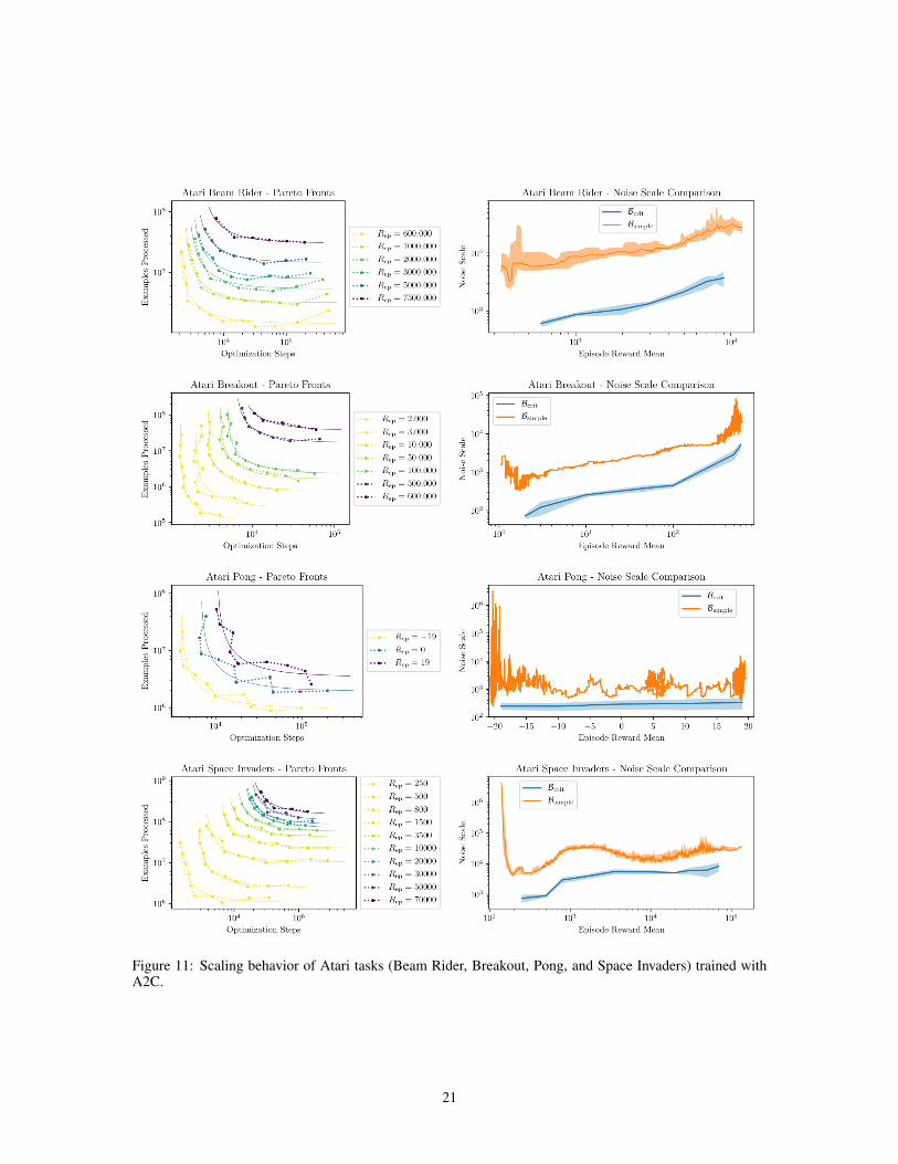
Figure 11: Scaling behavior of Atari tasks (Beam Rider, Breakout, Pong, and Space Invaders) trained withA2C.
21
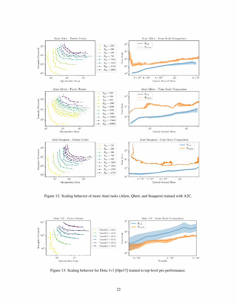
Figure 12: Scaling behavior of more Atari tasks (Alien, Qbert, and Seaquest) trained with A2C.
Figure 13: Scaling behavior for Dota 1v1 [Ope17] trained to top-level pro performance.
22

Figure 14: Scaling behavior of image classification tasks.
23

Critical Batch Size Simple Noise ScaleStart Average Start Average
Image Classification:MNIST 20 200 50 900SVHN 50 500 300 4,000CIFAR10 300 900 400 2,000ImageNet 1,000 15,000 4,000 30,000
Generative and Language Modeling:Autoencoder (SVHN) 10 40 2 2Variational Autoencoder (SVHN) 10 200 10 10Billion Word (per token) 700 100,000 1000 150,000
Reinforcement Learning:Atari (per frame) 100 - 1,000 400 - 8,000 100-1,000 1,000-20,000Dota 1v1 (per frame) 50,000 3,000,000 100,000 300,000Dota 5v5 (per frame) (not measured) >8,000,000 (est.) 100,000 24,000,000
Table 1: We report the simple noise scale, both early in training and averaged over a training run, as well asthe critical batch size, both early in the run and at the end of the run. The noise scale provides a good estimatefor the critical batch size throughout training. Batch sizes reported in number of images, tokens (for languagemodels), or observations (for games). These data are summarized in Figure 4.
24

Figure 15: The noise scale is proportional to the inverse temperature. On the left we display results for SVHNoptimized via SGD, while on the right we have an LSTM on the Billion Word dataset optimized via Adam.For each of the three curves, we modified either the learning rate ε, the batch size B, or both, so that thetemperature ε
B was decreased by a factor of 16 between epochs 1 and 1.5 (SVHN) or 0.02 and 0.03 (BW). Inall cases we see that the simple noise scale increased by a factor of 16, then returned to roughly its originalvalue once ε, B were reset.
C Temperature and the Noise Scale
The noise scale measured during neural network training could depend on a variety of hyperparameters, suchas the learning rate ε or momentum. However, we have empirically found that noise scale primarily dependson ε and B roughly through the ratio
T (ε, B) ≡ ε
εmax(B), (C.1)
which we refer to as the ‘temperature’ of training. The terminology reflects an idea of the loss as a potentialenergy function, so that high temperature training explores a larger range of energies.
In the case of pure SGD it is approximated by T ≈ ε/B in the small batch regime. Our definition of T canthen be obtained from a toy model of a quadratic loss, which is described below. In that case one can showexplicitly [MHB17] that the equilibrium distribution of gradients is characterized by this temperature13.
In equilibrium, the noise scales vary in proportion to the inverse temperature, so that
Bnoise ∝ Bsimple ∝1
T. (C.2)
It may seem surprising that higher temperature results in a smaller noise scale. The intuition is that at largerT the neural network parameters are further from the minimum of the loss, or higher up the ‘walls’ of thepotential, so that the gradient magnitude is larger relative to the variance.
Of course the loss landscape will be much more complicated than this toy model, but we have also observedthat this scaling rule provides a good empirical rule of thumb, even away from pure SGD. In particular, whenwe decay the learning rate ε by a constant factor, we often find that the noise scale grows by roughly thesame factor. ImageNet training provides an example in Figure 10. A more direct investigation of the relationbetween Bsimple and T is provided in Figure 15.
Since the noise depends primarily on the training temperature, and well-tuned training runs should have thesame temperature at different batch sizes, the measured noise scale will also be consistent between optimally-tuned runs at different batch sizes.14. The noise scale then depends only on the temperature and the loss.
13This definition can also be motivated by the empirical results of [SKYL17], which show that decaying the learningrate and increasing the batch size by the same factor have the same effect on training in the small-batch regime.
14This suggests that we can use the noise scale to define the temperature via Equation C.2. Then, once we have tunedthe learning rate and measured the noise scale at small batch size, we can tune the learning rate at larger batch sizes to thenoise scale constant. Though we have not investigated this idea thoroughly, it could significantly simplify the problem oflearning rate tuning at large batch size.
25
To summarize, the noise scale does not provide an optimal training temperature schedule, but it insteadprescribes an optimal batch size at any given temperature.
A Toy Model for the Temperature
Now let us consider a simple explanation for the behavior of the noise scale in response to changes in thelearning rate ε and batch size B. We start by approximating the loss as locally quadratic:
L (θ) =1
2θTHθ + const.
where we set θ = 0 at the minimum without loss of generality. To compute the noise scale, we need amodel for the gradient covariance matrix Σ. A simple model appearing in [SZL13] suggests treating the per-example loss Li as a shifted version of the true loss, Li (θ) = L (θ − ci), where ci is a random variable withmean zero and covariance matrix Σc. The gradient covariance matrix is then given by Σ = HΣcH , which isindependent of θ. The average gradient itself is given by G = Hθ, with θ changing in response to ε or B. Asshown in [MHB17] over sufficiently long times SGD15 will approximately sample θ from the distribution
pSGD (θ) ∝ exp
[−1
2θTM−1θ
]where the matrix M satisfies
MH +HM =ε
BΣ.
From these results, we can estimate the noise scale:
Bsimple =tr(Σ)
|G|2≈ B
ε
tr (Σ)
tr (H2Σ)
Bnoise =tr(Σ)H
GTHG≈ B
ε
tr (HΣ)
tr (H3Σ)
So, in this model, the noise scale is expected to increase as we decrease the learning rate or increase thebatch size. We also expect that scaling the learning rate and batch size together should leave the noise scaleunchanged.
WhenB � Bsimple, the ratio εB plays the role of a “temperature”. Since our analysis was only based on a toy
model optimized using pure SGD, one might not expect it to work very well in practice. However, as shownin Figure 15, we have found that it provides a quite accurate model of the dependence of the noise scale on εand B during neural network training, even when using the Adam16 optimizer. For these tests, on SVHN weused an initial (ε, B) = (0.18, 128) while for billion word results we used (ε, B) = (6× 10⁻⁴, 128).
Note that this result relies on the assumption that the optimizer has approached an effective equilibrium.We expect the equilibration timescale to be larger in the directions of low curvature, so that this effect willbe strongest when the gradient points mostly in the large-curvature directions of the Hessian. It would beinteresting to investigate the timescale for equilibration.
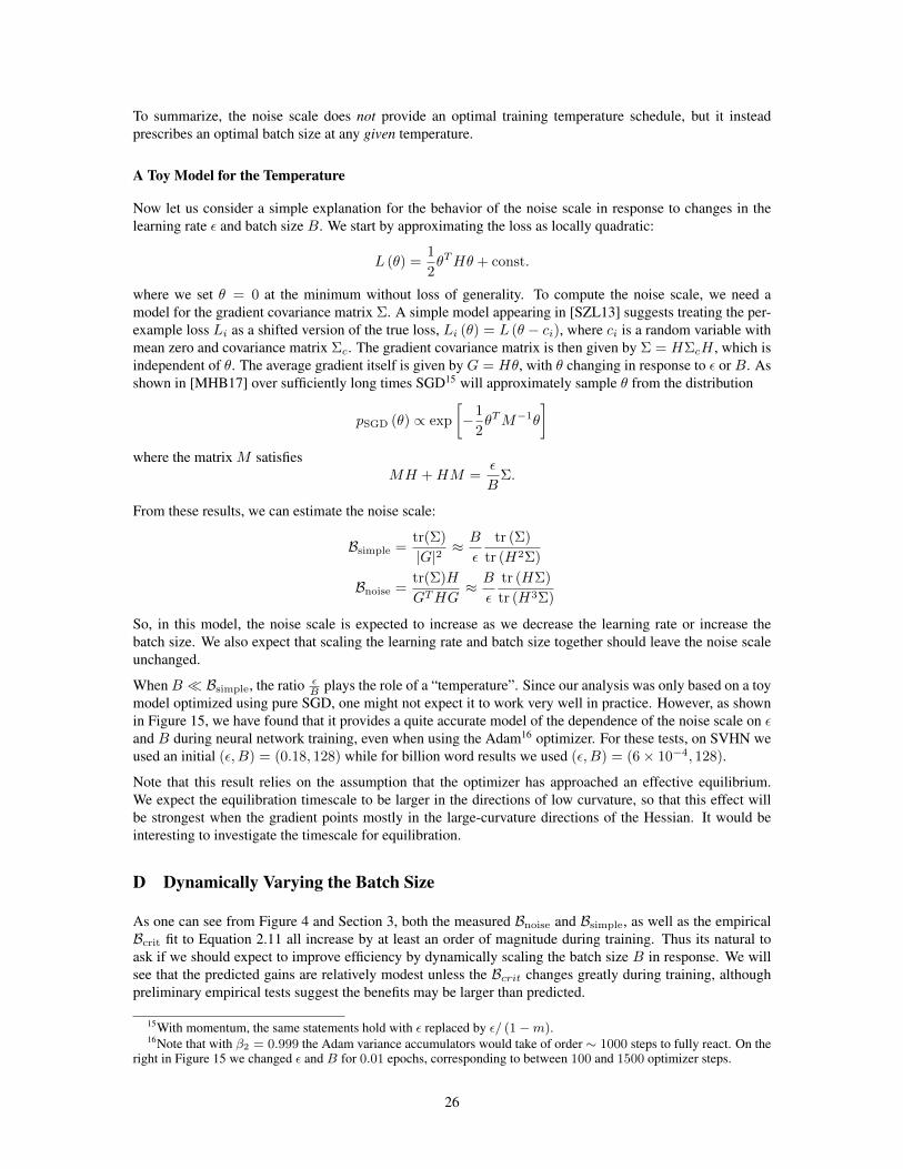
D Dynamically Varying the Batch Size
As one can see from Figure 4 and Section 3, both the measured Bnoise and Bsimple, as well as the empiricalBcrit fit to Equation 2.11 all increase by at least an order of magnitude during training. Thus its natural toask if we should expect to improve efficiency by dynamically scaling the batch size B in response. We willsee that the predicted gains are relatively modest unless the Bcrit changes greatly during training, althoughpreliminary empirical tests suggest the benefits may be larger than predicted.
15With momentum, the same statements hold with ε replaced by ε/ (1−m).16Note that with β2 = 0.999 the Adam variance accumulators would take of order ∼ 1000 steps to fully react. On the
right in Figure 15 we changed ε and B for 0.01 epochs, corresponding to between 100 and 1500 optimizer steps.
26
D.1 Theory
Consider a single full-batch optimizer step, over which the loss increases by an amount δL. If we instead usea batch of size B, it will take δS = 1 + B
B optimizer steps and δE = BδS training examples to make thesame amount of progress, where B is the noise scale. Over a full training run, the total number of steps anddata examples processed can be written as
S =
∫ (1 +B(s)
B(s)
)ds (D.1)
E =
∫(B(s) +B(s)) ds
where we parameterize the training trajectory by the number s of full-batch optimizer steps (we abbreviatedSmin above to s for notational simplicity).
The question is how to optimally distribute the training examples over the full training trajectory. At eachpoint along the trajectory, we have the choice of trading examples for optimizer steps by increasing or de-creasing the batch size. This “exchange rate” between examples and steps is
r = −ddB δEddB δS
=B2(s)
B(s). (D.2)
If the distribution of training examples (and hence the batch size schedule) is optimal, then transferringexamples from one part of training to another should not save any optimization steps. This means that theexchange rate r should be constant throughout training. Thus the batch size should be varied in proportionwith the square root of the noise scale:
B(s) =√rB(s). (D.3)
We can determine the resultant Pareto front parameterizing the tradeoff between training cost and time byinserting Equation D.3 into Equation D.1 and eliminating the exchange rate17
Stot
Smin− 1 = γ
(Etot
Emin− 1
)−1, (D.4)
where we define Smin ≡∫ds and Emin ≡
∫Bds to be the minimum possible number of optimizer steps
and training examples needed to reach the desired level of performance, obtained by inserting B � B andB � B respectively into D.3. We also define
γ ≡
(∫ √Bds
)2SminEmin
, (D.5)
which parameterizes the amount of variation of the noise scale over the course of training. When the noisescale is constant γ = 1 and there is no benefit from using an adaptive batch size; more variation in B pushes γcloser to 0, yielding a corresponding predicted improvement in the Pareto front.18 Note that since γ involvesthe variation in the square root of B, practically speaking B must vary quite a bit during training for adaptivebatch sizes to provide efficiency benefits via these effects. Adaptive batch sizes may also have other benefits,such as replacing adaptive learning rates [SKYL17] and managing the proportion of gradient noise duringtraining.
17The exchange rate r is a free parameter. It can be chosen according to preference from the value of training time vscompute. There is also the fairly natural choice r = Emin
Sminat which we have Stot
Smin= Etot
Emin= 1 +
√γ, so that cost-
efficiency and time-efficiency are both within the same factor of optimal, corresponding to the turning point in Figure16.
18To see explicitly the dependence of γ on the variability of the noise scale, we can rewrite it as γ =E[√B]2
E[B] =1
1+σ2√B/E[√B]2
, where the expectation is over a training run, weighting each full-batch step equally.
27

Figure 16: Left: We compare training using an adaptive batch size (data points) to the hyperbolic fit to Paretofronts at fixed batch size (lines). We note a modest but visible improvement to training efficiency. Adaptivebatch sizes appear to decrease the minimum number of optimization steps Smin, which was not anticipatedby theoretical analysis. Right: Depending on the degree to which the noise scale varies over training, we canpredict the potential Pareto improvement from using an adaptive batch size.
D.2 An SVHN Case Study
We have argued that a batch size of order the noise scale can simultaneously optimize data parallelism andtotal resource use. We have also shown that the noise scale tends to grow quite significantly during training.This suggests that one can further optimize resource use by adaptively scaling19 the batch size with the noisescale as training progresses, as discussed above.
For adaptive batch training, we can follow a simple and pragmatic procedure and dynamically set
B =√rBsimple, (D.6)
with Bsimple measured periodically during training. The results from dynamic batch training with this pro-cedure and various values of r are compared to fixed batch size training in Figure 16. We see that adaptivetraining produces a modest20 efficiency benefit.
We can combine our fixed batch size results with theoretical analysis to predict the magnitude of efficiencygains that we should expect from adaptive batch size training. We displayed Bcrit for fixed batch training ofSVHN in Figure 7. We have found that these results are fit very well by Bcrit(s) ≈ 10
√s, where s is the
number of steps taken in the limit of very large batch training. Using Equation D.5, we would predict thequite modest efficiency gain of
γ =
(∫ds 4√s)2
s∫ds√s
=24
25(D.7)
or around 4%. The benefits visible in Figure 16 in some cases appear too large to be fully explained by thisanalysis.
In particular, the adaptive batch size seems to benefit training in the regime of large batch size, decreasingthe minimum number of optimization steps Smin. However, our theoretical analysis would predict negligiblebenefits at large Etot/Stot. This may be due to the fact that the adaptive BS schedule also ‘warms up’the learning rate, or it may be an effect of a larger and more consistent proportion of gradient noise duringtraining. It would be interesting to disentangle these and other factors in future work, and to study adaptivebatch size training on other datasets.
19This may have an additional advantage compared to training with a fixed, large batch size: it allows for a constantproportion of gradient noise during training, and some have argued [KMN+16, HHS17] that noise benefits generalization.
20It’s challenging to provide a fair comparison between fixed and adaptive batch size training. Here we determineda roughly optimal relation ε = 0.27B
96+Bbetween learning rate ε and B for fixed batch size training, and used this same
function to determine the learning rate for both fixed and adaptive batch size training runs. This meant the adaptive batchsize training used a corresponding adaptive learning rate. We did not experiment with learning rate schedules.
28

Figure 17: Left: This figure shows the magnitude of the optimal step size in the direction of the parameterupdate divided by the magnitude of the actual update. Optimal step sizes are determined by a line search ofthe loss. We show training of two quite different models with different optimizers – an LSTM trained withAdam (momentum = 0.5) on Billion Word, and a CNN trained on SVHN with SGD. In both cases, trainingconverges to an approximate steady state where the average update is about twice the optimal update. Right:Learning curves included to clarify that this phenomenon is not due to the cessation of learning.
Figure 18: The gradient exhibits rapid, long-lived oscillations over the course of training, even when usingadaptive optimizers such as Adam. These oscillations are typical when optimizing functions with a large Hi-erarchy in the Hessian spectrum. We measure the moving average of the gradient with decay 0.5, computingits correlations over time. Results are shown for a simple CNN trained on SVHN using the Adam optimizer.
E Comments on Optimization
E.1 Deterministic Training Performs Poorly
From the discussion of the noise scale in Section 2, we expect that at large batch size B � Bnoise we canobtain a very good estimate of the gradient. This would then suggest a minimally stochastic approach totraining, where at each step one performs a line search of the true loss in the direction of the true gradient,and updates parameters accordingly.
This nearly deterministic ‘greedient descent’ method performs poorly in practice [WRLG18]. While its firstfew steps tend to decrease the loss significantly, subsequent step sizes decrease rapidly and provide minimalfurther training progress. In fact, when training with a fixed learning rate, we have observed that training
29

often tends towards a regime where the optimal step size (determined by a line search in the direction of theparameter update) is almost exactly half of the actual update magnitude. We have found that this phenomenonoccurs regardless of the learning rate (scanning over several orders of magnitude), and seems common to avariety of different models, as shown in Figures 17 and 18. A natural interpretation of these results is thatlarge Hessian directions are dominating the update [GARD18], so that training involves rapid oscillations, asseen in Figure 18 (see [Goh17] for an intuitive picture of these oscillations). Because of this, line searches donot appear to be useful in determining the optimal step size for a full training run.
E.2 Motivations for Learning Rate Scaling Rules
The learning rate scaling rule from Appendix A.2 can be motivated as follows. Equation A.3 generalizesEquation 2.6, which was derived for plain SGD. The SGD linear scaling rule (α = 1) means that the stepsize per data example stays fixed up to B∗; one might intuitively expect that this is necessary to avoid dimin-ishing returns as B increases. In the case of Adam21, we can use noise scale considerations to motivate thegeneralization to 0.5 < α < 1. The Adam update to the parameter θi takes the form
δθi = εEβ1
[Gi]√Eβ2 [G2
i ] + εAdam
where Eβ refers to an exponentially-weighted moving average with decay parameter β, and G refers to agradient from a batch of size B. If we disregard β1, β2, and εAdam, this is roughly equivalent to
δθi ≈ εsign (E [Gi])√
1 + siE[Gi]
2
.
where si is the variance of Gi over timesteps. If the step-to-step noise in the gradient is primarily due tobatch statistics, si should scale inversely with B. Comparing with 2.6, this implies a square-root scaling rule(α = 0.5) to maintain a constant learning rate per data example. However, since β2 is often set to large valuesaround 0.999, the second moment accumulator may not have time to adapt to quick changes in the gradientnoise; this pushes α back towards 1.0. This may explain the variation in α between different tasks.
E.3 Preliminary Tests of Generalization
Throughout the paper we have studied the noise scale as a function of the training loss or RL score. But fornon-RL tasks, it is also interesting to study the relationship between the noise scale and the critical batch sizeassociated with minimization of the test loss. The difference between the training and test results providesinformation about generalization. In Figure 19 we report results using the test loss for the small imageclassification datasets.
As expected, early in training there is no difference between train and test results. However, at the very end oftraining we observe a small dip in Bcrit for the test loss, which appears to occur consistently across datasets.It would be very interesting to further investigate this phenomenon in the future.
21These considerations apply equally well to RMSProp.
30
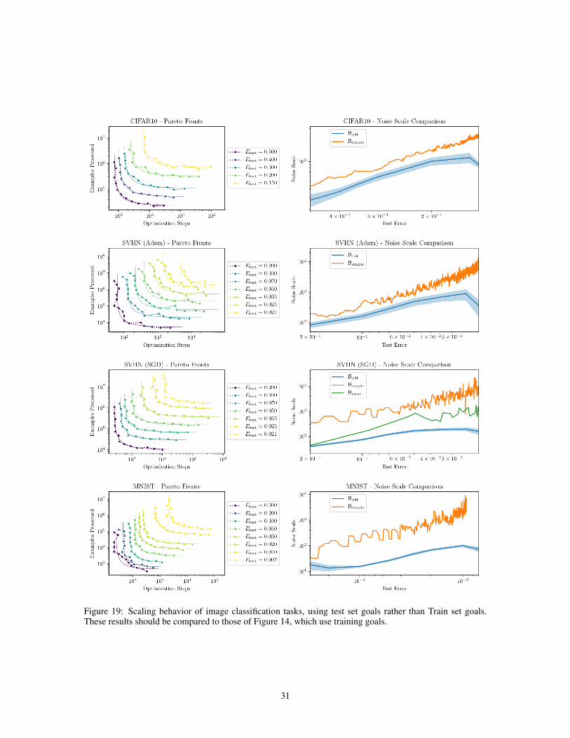
Figure 19: Scaling behavior of image classification tasks, using test set goals rather than Train set goals.These results should be compared to those of Figure 14, which use training goals.
31

References
[AAG+18] Igor Adamski, Robert Adamski, Tomasz Grel, Adam Jedrych, Kamil Kaczmarek, and HenrykMichalewski. Distributed deep reinforcement learning: Learn how to play atari games in 21minutes, 2018, 1801.02852. 2, 14
[AH18] Dario Amodei and Danny Hernandez. AI and Compute, May 2018. URL https://blog.
openai.com/ai-and-compute/. 2
[ASF17] Takuya Akiba, Shuji Suzuki, and Keisuke Fukuda. Extremely large minibatch sgd: Trainingresnet-50 on imagenet in 15 minutes, 2017, 1711.04325. 2
[BCD+18] Greg Brockman, Brooke Chan, Przemyslaw Debiak, Christy Dennison, David Farhi, RafalJózefowicz, Jakub Pachocki, Michael Petrov, Henrique Pondé, Jonathan Raiman, SzymonSidor, Jie Tang, Filip Wolski, and Susan Zhang. OpenAI Five, Jun 2018. URL https:
//blog.openai.com/openai-five/. 1, 2, 3, 9, 13, 14, 16, 19
[BCN16] Léon Bottou, Frank E. Curtis, and Jorge Nocedal. Optimization methods for large-scale machinelearning, 2016, 1606.04838. 14
[BCNW12] Richard H. Byrd, Gillian M. Chin, Jorge Nocedal, and Yuchen Wu. Sample size selection inoptimization methods for machine learning. Mathematical Programming, 134(1):127–155, Aug2012. doi:10.1007/s10107-012-0572-5. 14
[BCP+16] Greg Brockman, Vicki Cheung, Ludwig Pettersson, Jonas Schneider, John Schulman, Jie Tang,and Wojciech Zaremba. OpenAI Gym, 2016, 1606.01540. 19
[BDS18] Andrew Brock, Jeff Donahue, and Karen Simonyan. Large scale gan training for high fidelitynatural image synthesis, 2018, 1809.11096. 2
[BGM17] Jimmy Ba, Roger Grosse, and James Martens. Distributed second-order optimization us-ing kronecker-factored approximations, 2017. URL https://openreview.net/forum?id=
SkkTMpjex. 14
[BNVB12] Marc G. Bellemare, Yavar Naddaf, Joel Veness, and Michael Bowling. The arcade learningenvironment: An evaluation platform for general agents. CoRR, 2012, 1207.4708. 13, 19
[BRH16] Lukas Balles, Javier Romero, and Philipp Hennig. Coupling adaptive batch sizes with learningrates, 2016, 1612.05086. 14
[CDH+16] Xi Chen, Yan Duan, Rein Houthooft, John Schulman, Ilya Sutskever, and Pieter Abbeel. In-fogan: Interpretable representation learning by information maximizing generative adversarialnets, 2016, 1606.03657. 19
[CMS+13] Ciprian Chelba, Tomas Mikolov, Mike Schuster, Qi Ge, Thorsten Brants, Phillipp Koehn, andTony Robinson. One billion word benchmark for measuring progress in statistical languagemodeling, 2013, 1312.3005. 12, 19
[CWZ+18] Lingjiao Chen, Hongyi Wang, Jinman Zhao, Dimitris Papailiopoulos, and Paraschos Koutris.The effect of network width on the performance of large-batch training, 2018, 1806.03791. 14
[DDS+09] J. Deng, W. Dong, R. Socher, L.-J. Li, K. Li, and L. Fei-Fei. ImageNet: A Large-Scale Hier-archical Image Database. In CVPR09, 2009. URL http://www.image-net.org/papers/
imagenet_cvpr09.pdf. 12, 18
[DHK+17] Prafulla Dhariwal, Christopher Hesse, Oleg Klimov, Alex Nichol, Matthias Plappert, AlecRadford, John Schulman, Szymon Sidor, Yuhuai Wu, and Peter Zhokhov. Openai baselines.https://github.com/openai/baselines, 2017. 19
[DNG17] Aditya Devarakonda, Maxim Naumov, and Michael Garland. Adabatch: Adaptive batch sizesfor training deep neural networks, 2017, 1712.02029. 14
[DYJG16] Soham De, Abhay Yadav, David Jacobs, and Tom Goldstein. Big batch sgd: Automated infer-ence using adaptive batch sizes, 2016, 1610.05792. 14
[GARD18] Guy Gur-Ari, Daniel A. Roberts, and Ethan Dyer. Gradient descent happens in a tiny subspace.2018, arXiv:1812.04754. 30
32
[GDG+17] Priya Goyal, Piotr Dollár, Ross Girshick, Pieter Noordhuis, Lukasz Wesolowski, Aapo Kyrola,Andrew Tulloch, Yangqing Jia, and Kaiming He. Accurate, large minibatch sgd: Trainingimagenet in 1 hour, 2017, 1706.02677. 2, 14, 20
[Goh17] Gabriel Goh. Why momentum really works. Distill, 2017. doi:10.23915/distill.00006. 8, 30
[Goo] Google. Tensorflow official models. URL https://github.com/tensorflow/models/
tree/master/official/resnet. 18
[GVS14] Ian J. Goodfellow, Oriol Vinyals, and Andrew M. Saxe. Qualitatively characterizing neuralnetwork optimization problems, 2014, 1412.6544. 15
[GVY+18] Noah Golmant, Nikita Vemuri, Zhewei Yao, Vladimir Feinberg, Amir Gholami, Kai Rothauge,Michael W. Mahoney, and Joseph Gonzalez. On the computational inefficiency of large batchsizes for stochastic gradient descent, 2018, 1811.12941. 14
[HHS17] Elad Hoffer, Itay Hubara, and Daniel Soudry. Train longer, generalize better: closing the gener-alization gap in large batch training of neural networks. 2017, 1705.08741. 8, 28
[HMG07] Ralf Herbrich, Tom Minka, and Thore Graepel. TrueskillTM: A bayesian skill rating system.In B. Schölkopf, J. C. Platt, and T. Hoffman, editors, Advances in Neural Information Process-ing Systems 19, pages 569–576. MIT Press, 2007. URL http://papers.nips.cc/paper/
3079-trueskilltm-a-bayesian-skill-rating-system.pdf. 19
[HNA+17] Joel Hestness, Sharan Narang, Newsha Ardalani, Gregory Diamos, Heewoo Jun, Hassan Kia-ninejad, Md. Mostofa Ali Patwary, Yang Yang, and Yanqi Zhou. Deep learning scaling is pre-dictable, empirically, 2017, 1712.00409. 15
[HQB+18] Dan Horgan, John Quan, David Budden, Gabriel Barth-Maron, Matteo Hessel, Hado van Has-selt, and David Silver. Distributed prioritized experience replay, 2018, 1803.00933. 2, 14
[HS97] Sepp Hochreiter and Jürgen Schmidhuber. Long short-term memory. Neural Comput.,9(8):1735–1780, November 1997. doi:10.1162/neco.1997.9.8.1735. 19
[HZRS15] Kaiming He, Xiangyu Zhang, Shaoqing Ren, and Jian Sun. Deep residual learning for imagerecognition. CoRR, 2015, 1512.03385. 12, 18, 20
[IES+18] Andrew Ilyas, Logan Engstrom, Shibani Santurkar, Dimitris Tsipras, Firdaus Janoos, LarryRudolph, and Aleksander Madry. Are deep policy gradient algorithms truly policy gradientalgorithms?, 2018, 1811.02553. 14
[JSH+18] Xianyan Jia, Shutao Song, Wei He, Yangzihao Wang, Haidong Rong, Feihu Zhou, LiqiangXie, Zhenyu Guo, Yuanzhou Yang, Liwei Yu, Tiegang Chen, Guangxiao Hu, Shaohuai Shi, andXiaowen Chu. Highly scalable deep learning training system with mixed-precision: Trainingimagenet in four minutes, 2018, 1807.11205. 2, 12, 14
[KB14] Diederik P. Kingma and Jimmy Ba. Adam: A method for stochastic optimization, 2014,1412.6980. 5, 7, 12, 17, 18, 19
[KMN+16] Nitish Shirish Keskar, Dheevatsa Mudigere, Jorge Nocedal, Mikhail Smelyanskiy, and PingTak Peter Tang. On large-batch training for deep learning: Generalization gap and sharp minima,2016, 1609.04836. 8, 15, 28
[Kri09] Alex Krizhevsky. Learning multiple layers of features from tiny images. 2009. URL https:
//www.cs.toronto.edu/~kriz/learning-features-2009-TR.pdf. 12, 18
[KW13] Diederik P Kingma and Max Welling. Auto-encoding variational bayes, 2013, arXiv:1312.6114.12, 19
[LC10] Yann LeCun and Corinna Cortes. MNIST handwritten digit database. 2010. URL http:
//yann.lecun.com/exdb/mnist/. 12, 18
[LFLY18] Chunyuan Li, Heerad Farkhoor, Rosanne Liu, and Jason Yosinski. Measuring the intrinsicdimension of objective landscapes, 2018, 1804.08838. 8
[MBB17] Siyuan Ma, Raef Bassily, and Mikhail Belkin. The power of interpolation: Understanding theeffectiveness of sgd in modern over-parametrized learning, 2017, 1712.06559. 14
33

[MBM+16] Volodymyr Mnih, Adrià Puigdomènech Badia, Mehdi Mirza, Alex Graves, Timothy P. Lillicrap,Tim Harley, David Silver, and Koray Kavukcuoglu. Asynchronous methods for deep reinforce-ment learning. CoRR, 2016, 1602.01783. 13, 19
[MHB17] Stephan Mandt, Matthew D. Hoffman, and David M. Blei. Stochastic gradient descent as ap-proximate bayesian inference. 2017, 1704.04289. 14, 25, 26
[NIS] Selecting sample sizes. URL https://www.itl.nist.gov/div898/handbook/ppc/
section3/ppc333.htm. 14
[NVL+15] Arvind Neelakantan, Luke Vilnis, Quoc V. Le, Ilya Sutskever, Lukasz Kaiser, Karol Kurach,and James Martens. Adding gradient noise improves learning for very deep networks, 2015,1511.06807. 15
[NWC+11] Yuval Netzer, Tao Wang, Adam Coates, Alessandro Bissacco, Bo Wu, and Andrew Y. Ng.Reading digits in natural images with unsupervised feature learning. 2011. URL http://
ufldl.stanford.edu/housenumbers/nips2011_housenumbers.pdf. 12, 18
[OEGA18] Myle Ott, Sergey Edunov, David Grangier, and Michael Auli. Scaling neural machine transla-tion, 2018, 1806.00187. 2
[Ope17] OpenAI. More on Dota 2, Aug 2017. URL https://blog.openai.com/more-on-dota-2/.22
[PKYC18] Raul Puri, Robert Kirby, Nikolai Yakovenko, and Bryan Catanzaro. Large scale language mod-eling: Converging on 40gb of text in four hours, 2018, 1808.01371. 2
[SA18] Adam Stooke and Pieter Abbeel. Accelerated methods for deep reinforcement learning, 2018,1803.02811. 2, 14, 19
[SHB15] Rico Sennrich, Barry Haddow, and Alexandra Birch. Neural machine translation of rare wordswith subword units. CoRR, 2015, 1508.07909. 19
[SKYL17] Samuel L. Smith, Pieter-Jan Kindermans, Chris Ying, and Quoc V. Le. Don’t decay the learningrate, increase the batch size, 2017, 1711.00489. 2, 14, 25, 27
[SL17] Samuel L. Smith and Quoc V. Le. A bayesian perspective on generalization and stochasticgradient descent, 2017, 1710.06451. 14
[SLA+18] Christopher J. Shallue, Jaehoon Lee, Joe Antognini, Jascha Sohl-Dickstein, Roy Frostig, andGeorge E. Dahl. Measuring the effects of data parallelism on neural network training, 2018,arXiv:1811.03600. 8, 13, 14
[SMDH13] Ilya Sutskever, James Martens, George Dahl, and Geoffrey Hinton. On the importance ofinitialization and momentum in deep learning. In Proceedings of the 30th InternationalConference on Machine Learning, volume 28, pages 1139–1147, 17–19 Jun 2013. URLhttp://proceedings.mlr.press/v28/sutskever13.html. 18, 19
[SWD+17] John Schulman, Filip Wolski, Prafulla Dhariwal, Alec Radford, and Oleg Klimov. Proximalpolicy optimization algorithms. CoRR, 2017, 1707.06347. 13, 19
[SZL13] Tom Schaul, Sixin Zhang, and Yann LeCun. No more pesky learning rates. In ICML (3),volume 28 of JMLR Workshop and Conference Proceedings, pages 343–351. JMLR.org, 2013.URL http://jmlr.org/proceedings/papers/v28/schaul13.html. 14, 26
[SZT17] Ravid Shwartz-Ziv and Naftali Tishby. Opening the black box of deep neural networks viainformation, 2017, 1703.00810. 14
[Wik] Sample size determination. URL https://en.wikipedia.org/wiki/Sample_size_
determination#Estimation_of_a_mean. 14
[WRLG18] Yuhuai Wu, Mengye Ren, Renjie Liao, and Roger Grosse. Understanding short-horizon bias instochastic meta-optimization, 2018, 1803.02021. 8, 14, 29
[YGG17] Yang You, Igor Gitman, and Boris Ginsburg. Large batch training of convolutional networks,2017, 1708.03888. 2, 12, 14
34

[YPL+17] Dong Yin, Ashwin Pananjady, Max Lam, Dimitris Papailiopoulos, Kannan Ramchandran, andPeter Bartlett. Gradient diversity: a key ingredient for scalable distributed learning, 2017,1706.05699. 14, 15
[YZH+17] Yang You, Zhao Zhang, Cho-Jui Hsieh, James Demmel, and Kurt Keutzer. Imagenet training inminutes, 2017, 1709.05011. 2, 14
35