an empirical economic assessment of the costs and … · page 1 of 51 an empirical economic...
TRANSCRIPT
Finance and Economics Discussion SeriesDivisions of Research & Statistics and Monetary Affairs
Federal Reserve Board, Washington, D.C.
An Empirical Economic Assessment of the Costs and Benefits ofBank Capital in the US
Simon Firestone, Amy Lorenc and Ben Ranish
2017-034
Please cite this paper as:Firestone, Simon, Amy Lorenc and Ben Ranish (2017). “An Empirical Economic Assess-ment of the Costs and Benefits of Bank Capital in the US,” Finance and Economics Dis-cussion Series 2017-034. Washington: Board of Governors of the Federal Reserve System,https://doi.org/10.17016/FEDS.2017.034.
NOTE: Staff working papers in the Finance and Economics Discussion Series (FEDS) are preliminarymaterials circulated to stimulate discussion and critical comment. The analysis and conclusions set forthare those of the authors and do not indicate concurrence by other members of the research staff or theBoard of Governors. References in publications to the Finance and Economics Discussion Series (other thanacknowledgement) should be cleared with the author(s) to protect the tentative character of these papers.
Page 1 of 51
An Empirical Economic Assessment of the Costs and Benefits of Bank Capital in the US
Simon Firestone, Amy Lorenc, and Ben Ranish
This Version: March 31, 2017
We evaluate the economic costs and benefits of bank capital in the United States. The analysis is
similar to that found in previous studies though we tailor the analysis to the specific features and
experience of the U.S. financial system. We also make adjustments to account for the impact of liquidity
and resolution-related regulations on the probability of a financial crisis. The conceptual framework
identifies the benefits of bank capital with a lower probability of financial crises, which decrease
economic output. The costs of bank capital are identified with increases in banks’ cost of funding. These
increases are passed along to borrowers in the form of higher borrowing costs, resulting in a lower level
of economic output. Optimal capital levels maximize the difference between benefits and costs, or
maximizes net benefits. Using a range of empirical estimates, we find that optimal bank capital levels in
the United States range from just over 13 percent to over 26 percent.
We assess the benefits of bank capital through calculating (1) how the probability of a financial
crisis declines as the economy-wide level of bank capital increases and (2) the output cost of a financial
crisis. The probability of a financial crisis is estimated using a bottom up approach that uses bank-level
data from advanced economies and a top down approach that uses aggregate data from the same
economies. The output costs associated with a financial crisis are estimated by considering short-run and
long-run output costs. Short run costs are taken primarily from recent research by Romer and Romer
(2015) that is adjusted to focus more heavily on the experience of large, advanced economies which are
more similar to the United States. The long-run costs are estimated assuming that financial crisis either
have permanent or temporary but persistent effects. We find that the net present value of the output cost
of a financial crisis ranges from roughly 40 to 100 percent of annual GDP.
The costs of bank capital arise from the effect of capital on banks’ cost of funding. Bank equity is
more expensive than debt, but an increase in capital makes investing in banks less risky. Informed by
recent research that focuses on U.S. banks, we assume that a bit less than 50 percent of the increase in
capital costs is offset by the reduced risk of bank equity. Overall, our results suggest that if banks pass all
of the increase in funding costs onto borrowers then borrowing rates would increase by 0.07 percentage
points. We also consider a situation in which only half of the increase is passed onto borrowers.
Considering the benefits and costs of bank capital in the U.S. that we measure, the level of capital
that maximizes the difference between total benefits and total costs ranges from just over 13 percent to

Page 2 of 51
just over 26 percent. The reported range reflects a high degree of uncertainty and latitude in specifying
important study parameters that have a significant influence on the resulting optimal capital level, such as
the output cost of a financial crisis or the effect of increased bank capital on economic output. Finally, the
study discusses a range of considerations and factors that are not included in the cost-benefit framework
that could have a substantial impact on estimated optimal capital levels.

Page 3 of 51
Contents
I. Introduction ........................................................................................................................................... 4
II. Analytical Framework .......................................................................................................................... 9
III. Institutional Environment ............................................................................................................... 11
IV. The Economic Benefits of Bank Capital ......................................................................................... 13
a. Probability of a Financial Crisis ...................................................................................................... 13
b. Cost of Financial Crises .................................................................................................................. 23
c. Estimated Range of Benefits of Capital .......................................................................................... 32
V. Economic Costs of Bank Capital ........................................................................................................ 33
VI. Assessment of Net Benefits ............................................................................................................ 40
VII. Other Economic Benefits and Costs of Bank Capital ..................................................................... 45
VIII. Conclusion ...................................................................................................................................... 47
IX. References ....................................................................................................................................... 48

Page 4 of 51
I. Introduction
We perform an economic analysis of the long-run costs and benefits of different levels of bank capital,
and estimate optimal Tier 1 capital levels under a range of modelling assumptions. Under our framework,
we translate the level of capital into a probability of a financial crisis.1 The main benefit of bank capital,
under this framework, is to reduce the probability of a financial crisis as higher capital levels are
associated with less frequent crises. In particular, we multiply this probability by the estimated severity of
future US financial crises in order to estimate the aggregate economic benefits of bank capital. The
benefits of additional capital generally decrease as capital levels rise; the potential improvement from
reducing the frequency of crises becomes more limited as crises become more infrequent. The aggregate
economic costs of capital stem from an increase in banks’ cost of capital, which is passed along to
borrowers in the form of higher credit costs and lowers gross domestic product (GDP). These costs are
proportional to the increase in bank capital.
Because of several necessary assumptions and uncertainty about specific parameters, we provide ranges
of the economic costs and benefits resulting from many models rather than a single estimate of the net
effects. The greatest source of uncertainty in the net benefit we model arises from uncertainty around the
long-run effects of a crisis. There is also uncertainty regarding the extent to which banks can pass along
the costs of increased capital to borrowers. We examine different assumptions about these two effects.
The shaded region in Figure 1 shows a range for our estimated net benefits of additional capital (i.e.
marginal net benefits). At levels of capital up to about 13 percent, the shaded region lies above the
horizontal axis. This implies that our estimated range for the benefit of additional capital remains positive
until Tier 1 capital ratios reach 13 percent. For levels of capital between 13 percent and a bit above 25
percent, the shaded region overlaps the horizontal axis. This overlap implies that our estimated benefits of
additional capital over this range may be positive or negative, depending on the modeling assumptions
used.
1 Throughout the paper, unless otherwise noted, when we refer to capital we mean Tier 1 risk-based capital.

Page 5 of 51
Figure 1: Estimates of the Net Benefits of Additional Tier One Capital (Marginal Net Benefits of Capital)
The width of the shaded region in the plot represents uncertainty around our estimates of the benefits and
costs associated with the level of bank capital. The upper bound of this region represents our high
estimate of the benefits and low estimate of the costs of bank capital. Specifically, it assumes that the
effects of a financial crisis are permanent, and that banks only pass 50 percent of capital related cost
increases through to borrowers. The lower bound of this region represents our low estimate of the benefits
and high estimate of the costs. Specifically, it assumes that the effects of crises diminish gradually over
time, and that banks pass all capital related cost increases through to borrowers.2 We note that this plot
shows levels, rather than minimum required capital. Since banks generally hold a buffer above and
beyond the minimum required capital, we expect that optimal minimum capital requirements may be a bit
below the range shown above.
The plotted region is downward sloping, representing the fact that marginal benefits from increased
capital fall as capital increases, while the cost of increased capital remains constant. The red line where
the region intersects the horizontal axis represents the range of estimated optimal capital; the point at
2 The low estimate of benefits also incorporates an assumption that total loss-absorbing capacity (TLAC) regulations independently reduce the probability of financial crises by 30 percent. Our high estimate of benefits assumes that TLAC reduces only the cost of financial crises, but not their probability.

Page 6 of 51
which further capital reduces the net benefit. We find that optimal capital levels are uncertain, but likely
range between roughly 13 percent to over 25 percent.
Our framework for producing these estimates require that we model (1) the probability of financial crises
given the level of bank capital, (2) the cost of financial crises in terms of the present value of lost GDP,
(3) the impact of capital on lending spreads, and (4) the impact of lending spreads on long run GDP.
In order to predict the probability of a crisis under different levels of capital, we follow two approaches.
The “bottom-up” approach uses simulations of U.S. bank capital levels under shocks of different
severities. The “top-down” approach employs logistic regression with country-level data. We average the
results from these two approaches into a single estimate of the relationship between capital levels and the
probability of a financial crisis.
For calculating the cost of a financial crisis, we consider both short-term and long-run effects. As there
have been relatively few financial crises in the United States, we use research on all advanced economies.
We primarily rely on results from two studies. Furceri and Mourougane (2012) study the long-run effects
of financial crises on GDP for a variety of advanced countries, comparing potential output to actual
output. The gap between the two is the effect of the crisis. They estimate autoregressive growth equations,
using data from 1960 to 2008, and find that a financial crisis has a durable effect of reducing GDP by 2
percentage points. Romer and Romer (2015) create a new measure of financial crises based on semi-
annual Organisation for Economic Co-operation and Development (OECD) narratives about member
countries. Romer and Romer (2015) use this measure and regression analysis to calculate the short-term
effects of a financial crisis. We use results from Romer and Romer (2015) for the short term effects, and
Furceri and Mourougane (2012) for the long-run effects.
To calculate the effect of increased capital on GDP, we calculate the effect on a representative U.S.
bank’s weighted average cost of capital. We assume that either all or half of the increase is passed on to
borrowers in the form of a higher rate on loans, and use the Federal Reserve Board’s FRB/US
macroeconomic model to forecast the effect of an increase in lending rates on GDP.
The calculation of the effect of the level of capital on banks’ cost of capital depends on how responsive
the cost of banks’ equity is to changes in leverage. The intuition is that, as leverage decreases, the risk of
equity decreases, and so too should the required return. This intuition was formalized by Modigliani and
Miller (1958) in their Nobel Prize winning research on the irrelevance of capital structure. Whether the
“M&M” hypothesis applies to the banking sector has been debated by economists for some time. A
common approach to addressing this question is to measure whether bank equity’s covariance with the
market or “beta” falls when leverage decreases. Recent work on U.S. banks includes Kashyap, Stein, and

Page 7 of 51
Hanson (2010), who find such an M&M effect in general, and Clark, Jones, and Malmquist (2015), who
show the effect varies by time and bank size. In this study, we consider a range of so-called M&M effects
that are consistent with the findings of recent research on the U.S. banking system.
In addition to these effects, we also consider recent structural changes to bank regulation in the U.S. In
particular, we consider how requirements that increase the resolvability of failing firms, and liquidity
regulation as embodied by the Liquidity Coverage Ratio (LCR) and the Net Stable Funding Ratio (NSFR)
have increased the resilience of U.S. banks since the recent financial crisis. This increased resiliency will
decrease the likelihood and cost of future crises, although the extent of this impact is uncertain. We offer
adjustments to our baseline results accounting for these regulations whenever possible and appropriate.
As a final step, we compare the benefits of increased bank capital with its cost, and calculate a range of
potential values for optimal bank capital. We find that increasing bank capital beyond the current average
value of 12.5 percent of risk weighted assets (RWA) would have positive net benefits for the U.S.
economy.3 Optimal capital ratios are at least 13 percent, and may be even higher than 25 percent,
depending on model assumptions.
There is an extensive literature on financial crises in advanced economies and the relationship between
bank capital and macroeconomic risk. We compare our analysis with other key papers within the body of
the report. Our methodology builds on studies by the Basel Committee on Banking Supervision (BCBS)
(2010), the Bank of England (Brooks et al. 2015), and the Federal Reserve Bank of Minneapolis (2016).
All studies use the same basic framework; the effects of increased bank capital on the probability and
severity of a crisis are compared to the increase in loan rates and associated reduction in GDP level. The
BCBS study uses meta-analysis of the academic literature, combined with results from various country-
specific supervisory models, to quantify these effects. The Bank of England (2015) and Federal Reserve
Bank of Minneapolis (2016) use both the existing literature and substantial original data analysis for
calibration to the UK and U.S. economies.
Our approach differs from these studies in some significant ways. For example, we use adjustments and
controls to account for the effects of new liquidity requirements and resolution requirements for failing
firms. We also use Romer and Romer (2015) generalized least squares (GLS) estimates of the severity of
financial crises in order to reduce the result’s dependence on data from inherently more volatile and
smaller economies that are arguably less relevant to the United States, while the Bank of England uses
other methods to adjust for the presence of such countries in the sample. We provide estimates alternately
3 We compute an average Tier 1 capital ratio of 12.5 percent for the U.S. banking system using year-end 2015 data from Bankscope, from Bureau van Dijk.

Page 8 of 51
using both permanent and persistent but decaying effects of financial crises on GDP. Finally, unlike the
BCBS (2010) and Bank of England (2015) studies, we design the research to ensure, where possible, that
the analysis is tailored to the specific features of the U.S. financial system so that the results are relevant
for considering capital regulatory policy in the United States.
We summarize the results of our study alongside previous studies in Table 1. In Table 1, we report the
impact of increasing bank capital from its current average U.S. level of 12.5 percent of RWA to 13.5
percent. In the final column we also report the range of optimal capital levels found by each study.
Table 1: Effect of an Increase in Capital from 12.5% to 13.5% and Optimal Capital Ratios, Four Studies
Benefits: Reduction in Pr(Crisis)* Crisis Cost
(bp) 4
Costs: Reduction in
GDP (bp)
Optimal Bank Capital
Federal Reserve Board (this study) 8 to 27 4 to 7 13% to 25+% BCBS (2010) ~3 to 24 9 9% to 15+%5 Bank of England (2015) ~2 to 10 1 to 5 10% to 14% Federal Reserve Bank of Minneapolis (2016) ~11 ~6 22%
Our results imply larger optimal capital levels than the Bank of England (2015), and similar levels to the
BCBS (2010) and Federal Reserve Bank of Minneapolis (2016) studies. The Bank of England study
arrives at a lower optimal capital level in large part because of a 30 percent reduction in the estimated
probability of crisis and a 60 percent reduction in the estimated cost of crisis that they attribute to the role
of Total-Loss Absorbing Capacity (TLAC). The Federal Reserve Bank of Minneapolis (2016) arrives at
an optimal capital level near the upper end of our range. While they find a relatively small impact of
capital on the probability of a crisis, they use a significantly higher estimate of the cost of financial crises
and an estimate of the economic costs of bank capital that is similar to our low estimate.
4 The range reported for benefits of capital in BCBS comes from the difference in the benefits at 12 percent and 13 percent TCE/RWA ratios under the alternative assumptions of cost of crises of 19 and 158 percent (Table 8). Bank of England figures for benefits use approximate changes in the after TLAC crisis probabilities at mid-cycle and peak from Table 7, multiplied by a 43 percent cost of financial crises. Minneapolis cost of a crisis is 158 percent. We approximate the reduction in the probability of crisis as 7bp based on the 69bp reduction in probability of a bailout between capital levels of 10 and 20 percent (Table 2). 5 The reported figure represents a ratio of Basel II tangible common equity (TCE) to risk-weighted assets. Table 8 of the BCBS report indicates that net benefits of capital requirements are maximized TCE to risk-weighted asset ratios ranging from 9 percent (no permanent effect of financial crises) to over 15 percent (large permanent effect of financial crises). Our analysis suggests the equivalent figures for the Tier 1 capital ratio would be 9.3 percent to 15.5+ percent.
Page 9 of 51
II. Analytical Framework
Our framework for measuring the long-run net benefits of bank capital levels follows previous work by
the BCBS (2010), Miles et al. (2013), Bank of England (2015), and the Federal Reserve Bank of
Minneapolis (2016).6 In the interest of simplicity, this framework allows bank capital to affect the
economy via just two channels: (1) the probability that a financial crisis starts and (2) banks’ cost of
capital. By using this framework, we do not incorporate the impact of capital on risk premia or lenders’
behavior. In addition, we do not measure benefits accruing to other economies, or benefits in the form of
increased utility of risk averse consumers. Section VII discusses these issues in further detail. With this
two-channel framework, the benefits of bank capital arise from a lower probability of financial crisis
related output gaps. The costs of bank capital are a lower equilibrium level of output, through the effect of
banks’ cost of capital on lending spreads. By subtracting the costs from the benefits, expressing both as a
percentage of annual GDP, we arrive at the equation below.
𝑁𝑁𝑁𝑁𝑁𝑁 𝐵𝐵𝑁𝑁𝐵𝐵𝑁𝑁𝐵𝐵𝐵𝐵𝑁𝑁𝐵𝐵 𝑜𝑜𝐵𝐵 𝐵𝐵𝐵𝐵𝐵𝐵𝐵𝐵 𝐶𝐶𝐵𝐵𝐶𝐶𝐵𝐵𝑁𝑁𝐵𝐵𝐶𝐶
= 𝑅𝑅𝑁𝑁𝑅𝑅𝑅𝑅𝑅𝑅𝑁𝑁𝐵𝐵𝑜𝑜𝐵𝐵 𝐵𝐵𝐵𝐵 𝑃𝑃𝑃𝑃𝑜𝑜𝑃𝑃𝐵𝐵𝑃𝑃𝐵𝐵𝐶𝐶𝐵𝐵𝑁𝑁𝑃𝑃 𝑜𝑜𝐵𝐵 𝐵𝐵 𝐹𝐹𝐵𝐵𝐵𝐵𝐵𝐵𝐵𝐵𝑅𝑅𝐵𝐵𝐵𝐵𝐶𝐶 𝐶𝐶𝑃𝑃𝐵𝐵𝐵𝐵𝐵𝐵𝐵𝐵 ���������������������������������increasing with capital (see section IV.a)
𝑋𝑋𝑁𝑁𝑁𝑁𝑁𝑁 𝑃𝑃𝑃𝑃𝑁𝑁𝐵𝐵𝑁𝑁𝐵𝐵𝑁𝑁 𝐶𝐶𝑜𝑜𝐵𝐵𝑁𝑁 𝑜𝑜𝐵𝐵 𝐵𝐵 𝐹𝐹𝐵𝐵𝐵𝐵𝐵𝐵𝐵𝐵𝑅𝑅𝐵𝐵𝐵𝐵𝐶𝐶 𝐶𝐶𝑃𝑃𝐵𝐵𝐵𝐵𝐵𝐵𝐵𝐵 (% 𝑜𝑜𝐵𝐵 𝐺𝐺𝐺𝐺𝑃𝑃)�����������������������������������unaffected by capital (see section IV.b)
− % 𝑅𝑅𝑁𝑁𝑅𝑅𝑅𝑅𝑅𝑅𝑁𝑁𝐵𝐵𝑜𝑜𝐵𝐵 𝐵𝐵𝐵𝐵 𝐺𝐺𝐺𝐺𝑃𝑃 𝐺𝐺𝑅𝑅𝑁𝑁 𝑁𝑁𝑜𝑜 𝐻𝐻𝐵𝐵𝐻𝐻ℎ𝑁𝑁𝑃𝑃 𝐿𝐿𝑁𝑁𝐵𝐵𝑅𝑅𝐵𝐵𝐵𝐵𝐻𝐻 𝑆𝑆𝐶𝐶𝑃𝑃𝑁𝑁𝐵𝐵𝑅𝑅𝐵𝐵�������������������������������������increasing with capital (see section V)
As mentioned above, banks generally keep buffers of capital above minimum requirements, so optimal
bank capital requirements would be lower than the capital levels shown below.
Figure 2 illustrates our basic solution concept for finding the optimal level of bank capital. As in the other
papers using this framework, the benefits of additional (marginal) capital that we estimate are decreasing
as capital rises, and eventually approach zero.7 This decrease can be seen in the downward slope of the
blue marginal benefits curve on the right-hand side plot.
Intuitively, at higher levels of capital there are fewer shocks left that are large enough to generate a crisis.
However, the costs of marginal capital that we estimate increase linearly. As a result, the marginal net
benefits in our framework steadily decrease and become negative beyond some level of capital K* that
represents optimal capital. As mentioned above, banks generally keep buffers of capital above minimum
requirements, so optimal bank capital requirements would be lower than the capital levels shown below.
6 The International Monetary Fund’s (IMF’s) analysis (Dagher et al. 2016) follows a similar framework but does not estimate of the cost of financial crises or net benefits. 7 Certain models of Miles et al. (2013) are an exception here as they use a bimodal distribution of financial system shocks.

Page 10 of 51
Figure 2: Relationship of Benefits, Costs, and Optimal Capital Level (K*)
The remainder of this study is devoted to conducting analysis designed to provide estimates of the
marginal benefit and marginal cost curves that are pictured in the right-hand panel of Figure 2. As
discussed previously, a variety of data and models are employed in estimating these relationships. This
study attempts to focus on data that is most relevant to the experience of the United States while
acknowledging that a variety of different models would produce varying results for the estimated
marginal benefit and cost curves. In addition it is worth noting that the analytical framework used to
determine optimal capital levels is rather stylized and abstracts from a number of real world
considerations.
In particular, our framework addresses broad changes in capital rather than targeted requirements that
apply to specific banks such as the global systemically important banks (GSIBs) surcharge and the
Comprehensive Capital Analysis and Review (CCAR).8 Our framework assumes that all banks choose the
same capital ratios, and we do not account for the heterogeneity of the U.S. capital framework resulting
from targeted regulations. It is possible that this heterogeneity could affect both estimated costs and
benefits. For example, if only certain banks were affected by higher capital ratios, a smaller share of their
increased cost of capital might be passed on to borrowers, decreasing the economic costs of the extra
dollar of capital. On the benefits side, additional capital has the greatest effect on the probability of failure
for the least well capitalized banks. Therefore, the microprudential benefits may be lower under
heterogeneous requirements. However, there may be greater macroprudential benefits in reducing the
failure rate of systemically important firms.
At the same time, this framework has been employed by all of the previous studies that have been
conducted in this area and so its use here reflects its widespread adoption in the academic literature and
8 See www.federalreserve.gov/newsevents/press/bcreg/20150720a.htm for more information on the GSIB surcharge. See www.federalreserve.gov/bankinforeg/stress-tests-capital-planning.htm.for more information on CCAR.

Page 11 of 51
also facilitates comparison with those studies. Future analyses may benefit from considering richer and
more complex models that consider important effects not captured in this framework.
Section III discusses the institutional environment in which our analysis takes place. In particular, many
new regulations have been adopted in the wake of the recent financial crisis that need to be accounted for
in our analysis. The rest of the paper is arranged as follows in order to build upon the analytical
framework. The economic benefits and costs of bank capital are estimated in Sections IV and V,
respectively. Section VI uses the results of the prior two sections to assess the net benefits of capital. We
discuss economic benefits and costs of capital not explicitly captured by our analysis in Section VII and
Section VIII concludes.
III. Institutional Environment
Two new U.S. enhancements to large bank safety and soundness will affect the relationship between bank
capital levels and the macro-economy: increased resolvability of failing firms and liquidity requirements.
In our analysis, we consider the effects of capital in the presence of both.
A number of resolution planning requirements have been adopted in order to ensure rapid and orderly
resolution in the event of financial distress or failure of a company. Of particular importance are the long-
term debt requirement and the TLAC requirement. These requirements are designed to create a source of
funds for recapitalization.9 They apply to top-tier U.S. bank holding companies that have been designated
as GSIBs and U.S. intermediate holding companies (IHCs) of foreign GSIBs. These institutions must
maintain a certain amount of eligible long-term unsecured debt that can be converted to equity for the
purpose of absorbing losses or recapitalization in the event of failure. Requirements are effective as of
January 1, 2019. The aggregate TLAC shortfall for U.S. GSIBs was estimated at $70 billion as of the
third quarter of 2016 (Total Loss-Absorbing Capacity 2016).
TLAC’s most direct effect will be a change from public “bail-outs” for large banks that are in severe
stress to private “bail-ins,” where the eligible debt held by private-sector creditors is converted into
equity. Such a mechanism is designed to quickly resolve distressed banks by rapidly providing a new
source of capital rather than resorting to taxpayer support.
9 See www.federalreserve.gov/newsevents/press/bcreg/20151030a.htm for more information on the long-term debt and TLAC requirements. See www.federalreserve.gov/bankinforeg/resolution-plans.htm for more information on living wills. See www.fdic.gov/regulations/laws/federal/2011/11finaljuly15.pdf for more information on the orderly liquidation authority.
Page 12 of 51
In addition to complying with the long-term debt and TLAC requirements, U.S. bank holding companies
with total consolidated assets of $50 billion or more must submit annual orderly resolution plans,
commonly known as living wills, to the Federal Reserve. These plans should facilitate the rapid and
orderly resolution of a firm in the event of failure and prevent contagion among broader financial
markets.
Beyond resolution planning requirements, the orderly liquidation authority (OLA) provided to the Federal
Deposit Insurance Corporation (FDIC) by Title II of the Dodd-Frank Wall Street Reform and Consumer
Protection Act of 2010 increases the resolvability of financial firms. The OLA provides an alternative to
standard bankruptcy that allows the FDIC to carry out the liquidation of a failing financial company,
aiming to minimize systemic risk and moral hazard.
We account for the benefits associated with increased resolvability of failing firms whenever possible.
We model a projected reduction in the length of a crisis, based on work by Homar and van Wijnbgergen
(2016), and find it reduces the expected cost. We also consider the effects of possible reductions in the
probability of a crisis due to reduced bank risk-taking.
Liquidity requirements are designed to permit a bank to maintain sufficient liquid assets during a period
of stress. There are two main liquidity requirements: a short-term Liquidity Coverage Ratio (LCR) and a
long-term Net Stable Funding Ratio (NSFR).10 The LCR was adopted in the United States in 2014, with
all phase-in to be completed by January 2017. It applies in full to all U.S. institutions with at least $250
billion in total assets or at least $10 billion in on-balance sheet foreign assets. Less stringent requirements
apply to institutions with between $50 billion and $250 billion in total assets and less than $10 billion in
on-balance sheet foreign assets. The LCR requires banks to maintain an amount of high-quality liquid
assets (HQLA) sufficient to cover expected net cash outflows during a 20-day stress period. HQLA is a
weighted sum of specific high quality liquid assets, with higher weights on the most liquid assets.
Expected net cash outflows are fixed by regulation and based on the type of liabilities. Shorter term and
more runnable liabilities are associated with the highest outflow rates.
The NSFR also has a two-tiered approach for institutions, based on the same total and foreign asset
thresholds. It is designed to ensure sufficient liquidity over a one-year horizon, compared with the 30 day
horizon of the LCR. It also requires an appropriate match between assets and liabilities. NSFR
requirements were the subject of a Notice of Proposed Rulemaking in April 2016. Almost all covered
10 See www.federalreserve.gov/newsevents/press/bcreg/20140903a.htm for more information on the LCR and www.federalreserve.gov/newsevents/press/bcreg/20160503a.htm on the NSFR.
Page 13 of 51
institutions as of December 2015 were already in compliance with the NSFR, and the few that were not
had relatively small shortfalls.
Shocks to the value of financial system assets are amplified by liquidity shortfalls. Banks with short-term
funding requirements exceeding their liquid assets may find themselves vulnerable to “fire sales” of
illiquid assets when such shocks occur. These sales can trigger losses, loss of funding liquidity, and asset
sales at other banks, potentially threatening the solvency of the entire system.11 Consequently, liquidity
requirements are also likely to reduce the probability of a financial crisis. We include adjustments for the
effect of liquidity regulations in our estimated financial crisis probabilities.
IV. The Economic Benefits of Bank Capital
As in past studies (BCBS 2010; Miles et al. 2013; Bank of England 2015; Federal Reserve Bank of
Minneapolis 2016), we measure the benefit of bank capital by first estimating bank capital’s role in
reducing the probability of a financial crisis (Section IV.a), and then multiplying this by the cost of
financial crises (Section IV.b). Our estimates are tailored where possible to the specifics of the U.S.
financial system, and include adjustments to account for the impact of additional liquidity and loss
absorption requirements on the marginal benefit of bank capital.
We rely on definitions of financial crises developed in previous surveys, as defining crises is a non-trivial
exercise. When estimating the probability of financial crises, we rely on the criteria and crises identified
by Laeven and Valencia (2012). When estimating the cost of financial crises, we use results from Romer
and Romer (2015), who develop a continuous narrative-based measure of financial distress. Romer and
Romer (2015) include an extensive comparison of their definition with that in Laeven and Valencia
(2012). They are almost equivalent in identifying if crises occur, but have a few differences with regard to
the crisis start dates.
We discuss additional, potentially significant, benefits of bank capital not captured in this framework in
Section VII.
a. Probability of a Financial Crisis
As with past studies, we estimate the probability of a financial crisis starting via two approaches with
distinct strengths and weaknesses; a “bottom-up” bank-level simulation and a “top-down” country level
regression. In our reported results, we use the average of the probabilities generated by the two
11 See Shleifer and Vishny (2011) for a review of the literature on asset fire sales. See Brunnermeier and Pedersen (2009) for a discussion of the destabilizing link between market and funding liquidity.

Page 14 of 51
approaches.12 For use in both approaches, we collect data spanning 24 developed OECD countries over
the period 1988 through 2014.13 These data include 23 of the financial crises identified by Laeven and
Valencia (2012). In both approaches, we estimate the long-run average effect of bank capital on financial
crises, whereas the Bank of England (2015) analysis estimates the impact at the peak and trough of credit
cycles separately and later combine these.
In the bottom-up approach we use bank-level data to simulate shocks to U.S. banks’ capital. We estimate
how frequently these shocks would be large enough to start a financial crisis at different levels of starting
capital. Specifically, our simulations assume that a financial crisis occurs whenever the capital shortfall
exceeds 3 percent of GDP, which is the definition used by the Bank of England (2015), and is the
threshold for “significant restructuring costs” used by Laeven and Valencia (2012). This approach
recognizes that the amount of capital required to avoid crises varies across historical stress periods. Since
losses in some historical episodes were very high, the probability of crisis in the bottom-up approach does
not become very small until capital levels reach relatively high levels. However, this approach does not
predict or account for financial crises whose proximate causes are other than the loss of capital.
The Bank of England (2015) impact study also includes a simulation of bank income, though the details
of their simulation differ, such as the relationship between the draws of income for different banks. The
International Monetary Fund (IMF) (Dagher et al. 2016) and Federal Reserve Bank of Minneapolis
(2016) also rely on what is essentially a bottom-up approach as well, but use country-level data on non-
performing loans instead of bank-level data on net income.
In the top-down approach we use historical country-level data to estimate the probability of a financial
crisis given the financial system’s capitalization, liquidity, and economic conditions. This approach
applies the less rigid definition of financial crisis developed by Laeven and Valencia (2012). Also, by
abstracting away from bank-level distress, the top-down approach implicitly focuses on the macro-
prudential role of capital regulations. Key data are unavailable for many countries in our sample, so we
estimate two separate regression specifications as a compromise. In one, we use the full sample, with a
more limited set of control variables. In the other, we use a larger set of control variables, but only over
the subsample where these variables are available. The average of the predictions from the two models is
used as our top-down estimate.
12 We apply a 50 percent weight to our bottom-up approach, and a 25 percent weight to each of the two models we rely on in our top-down approach. 13 The sample includes Australia, Austria, Belgium, Canada, Denmark, Finland, France, Germany, Greece, Iceland, Ireland, Italy, Japan, Luxembourg, the Netherlands, New Zealand, Norway, Portugal, Spain, Sweden, Switzerland, Turkey, the United Kingdom, and the United States.
Page 15 of 51
The Bank of England (2015) impact study employs a top-down regression that differs from one of our
specifications only to the extent that our variable definitions and coverage are a bit different. BCBS
(2010) also employs a range of similar reduced form models within the set of estimates they present.
The two sections that follow describe each of these approaches and the results they deliver in greater
detail.
Bottom-Up Approach
In this approach, we simulate net income for U.S. banks and then determine whether the aggregate capital
shortfall that results is large enough to classify as a financial crisis using the definition of “financial
crisis” that was described previously. In the process, we adjust the simulated income to account for the
fact that large U.S. banks are now subject to liquidity requirements as well. This adjustment is discussed
in more detail below.
To implement this approach, we use bank-level data on total assets, risk-weighted assets, net income, Tier
1 capital, and asset liquidity ratios from Bankscope, from Bureau van Dijk. These data have good
coverage over the period spanning 1988 through 2014.14
We use these historical data to simulate net income for U.S. banks. For each simulation, we first
randomly pick a single country-year scenario; for example, “France 2008.” Then, for each of the 5,935
U.S. banks at the end of 2015, we randomly draw (with replacement) a value for two-year net income /
RWA from within the set of large banks present in that country-year scenario.15,16 We use two-year net
income to roughly match the length of CCAR stress periods. This captures the fact that bank losses are
predictable over multiple years in stress periods, possibly because of the smoothing of asset value shocks
on balance sheets. We exclude small banks from the distribution of net income we draw from, as this
distribution may be different for small banks.17
Next, we compute the aggregate capital shortfall that results under the simulated net income draws and a
range of initial Tier 1 capital levels. We follow the Bank of England’s approach by identifying crises as
14 We exclude 30 country-years where coverage either appears particularly incomplete and/or includes banks representing less than $10 billion in aggregate total assets. 15 In contrast to our approach, the Bank of England impact analysis pools country-years into just two scenarios: one where credit/GDP and equity volatility are high, and one where they are not. 16 In order to account for the average difference between Basel III risk weights and risk weights under Basel I and II regimes, we increase risk weighted assets for all years prior to 2011 by the increase in U.S. average risk weights over 2011 to 2015 (about 11 percent). For 2012 through 2014, we increase risk-weighted assets by the increase in U.S. average risk weights between that year and 2015. 17 We define the cutoff between small and large banks so that 90 percent of each country’s financial system assets in each year are within “large” banks. Across countries, we have an average of about 915 large banks per year.

Page 16 of 51
simulations where the aggregate shortfall exceeds three percent of GDP (or $540 billion), or a significant
recapitalization as defined by Laeven and Valencia (2012). This shortfall is measured relative to a
threshold of 8.24 percent. This threshold is chosen so that the average probability of crisis generated by
the model when applied to the United States (1989 through 2014) equals the advanced economy average
probability of crisis (4.0 percent per Laeven and Valencia 2012).18 With our shortfall threshold and crisis
definition, if all U.S. banks had the same Tier 1 capital ratios, a crisis occurs whenever this ratio falls
below about 4.7 percent. We run our simulation 10,000 times, in each one using a random set of net
income draws from a randomly selected country-year scenario as described above.
For most of the historical data period, major liquidity regulations (LCR and NSFR) were not in effect. If
they were, banks may have had more liquid assets to sell off during stress periods, reducing the extent of
loss magnifying fire sales. To account for the effect of liquidity regulations on loss magnitudes, we use
the following procedure outlined below.
First, we construct a set of proxies for LCR compliance, as these figures are generally not available
historically.19 We identify a cross-section of 12 large U.S. banks in 2012 for which both LCR and liquid
asset share (from Bankscope) are available. The correlation of these two variables is significant (about
0.52), and a least squares regression of LCR on liquid asset share (without an intercept) yields:
LCR=2.55*liquid_asset_share. For each of these 12 observations, we then estimate the liquid asset share
required to set LCR equal to one (the required level) as: required_liquid_asset_share=(1-LCR)/2.55.
These 12 values are proxies for the liquid asset share equivalent to LCR compliance.
Next, we estimate the historical relationship between the (lagged) liquid asset share of a bank, and the
magnitude of banks’ losses. We run least squares regressions of the log magnitude of losses (relative to
RWA) on log liquid assets, alternately controlling for (lagged) log assets and bank type in addition to log
assets. The estimated coefficient on log liquid assets varies from -0.095 to -0.107, so we use -0.10 as our
estimate of the impact of log liquid assets on log loss magnitude.20
18 When using a different threshold, such as is done by the Bank of England, additional adjustments are required in order to match the historical frequency of financial crises. 19 We focus on LCR compliance as we lack decent proxies for the NSFR in our Bankscope data. 20 Depending on the specification, this coefficient is statistically significant at the 5 or 10 percent level with standard errors clustered at the country level. We treat this result with caution as we have not controlled for the fact that liquidity is an endogenous decision by banks. There is to our knowledge very little empirical work on the relationship between balance sheet liquidity and loss severity. Cifuentes, Ferrucci, and Shin (2005) use simulations and find that liquidity ratio requirements can limit “contagion” of bank failures because of illiquid asset fire sales. Malherbe (2014) finds in a theoretical model that liquidity ratio requirements can increase the probability of a financial crisis.
Page 17 of 51
To integrate these findings within the simulations described above, we draw the liquid asset share in
addition to the net income (relative to RWA) from the banks in each country-year scenario. We also
randomly assign one of the 12 proxies for LCR compliance based on liquid asset share to each bank.
Then, if the net income draw is negative and the liquid asset share drawn is less than the assigned LCR
proxy, net income is adjusted toward zero based on the relationship of log liquid assets to log loss
magnitude estimated above.
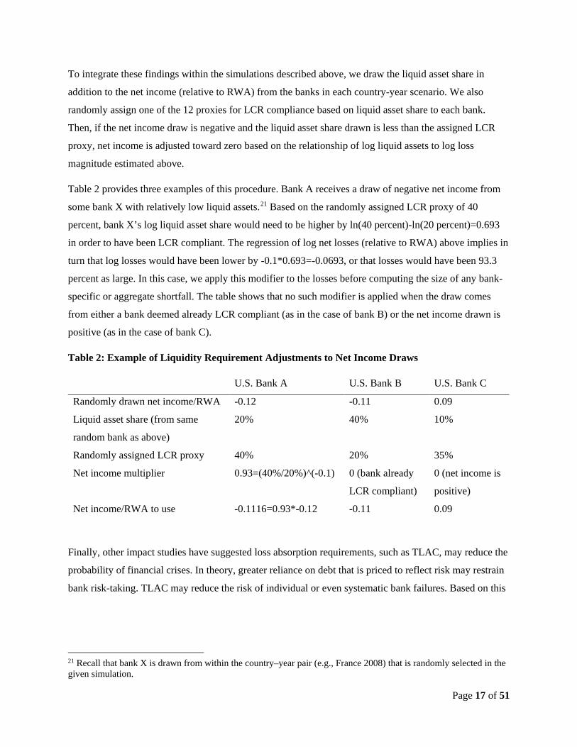
Table 2 provides three examples of this procedure. Bank A receives a draw of negative net income from
some bank X with relatively low liquid assets.21 Based on the randomly assigned LCR proxy of 40
percent, bank X’s log liquid asset share would need to be higher by ln(40 percent)-ln(20 percent)=0.693
in order to have been LCR compliant. The regression of log net losses (relative to RWA) above implies in
turn that log losses would have been lower by -0.1*0.693=-0.0693, or that losses would have been 93.3
percent as large. In this case, we apply this modifier to the losses before computing the size of any bank-
specific or aggregate shortfall. The table shows that no such modifier is applied when the draw comes
from either a bank deemed already LCR compliant (as in the case of bank B) or the net income drawn is
positive (as in the case of bank C).
Table 2: Example of Liquidity Requirement Adjustments to Net Income Draws
U.S. Bank A U.S. Bank B U.S. Bank C
Randomly drawn net income/RWA -0.12 -0.11 0.09
Liquid asset share (from same
random bank as above)
20% 40% 10%
Randomly assigned LCR proxy 40% 20% 35%
Net income multiplier 0.93=(40%/20%)^(-0.1) 0 (bank already
LCR compliant)
0 (net income is
positive)
Net income/RWA to use -0.1116=0.93*-0.12 -0.11 0.09
Finally, other impact studies have suggested loss absorption requirements, such as TLAC, may reduce the
probability of financial crises. In theory, greater reliance on debt that is priced to reflect risk may restrain
bank risk-taking. TLAC may reduce the risk of individual or even systematic bank failures. Based on this
21 Recall that bank X is drawn from within the country–year pair (e.g., France 2008) that is randomly selected in the given simulation.

Page 18 of 51
argument, the Financial Stability Board (2015) relies on work by Afonso et al. (2014) and Marques et al.
(2013) to estimate that TLAC reduces the probability of financial crises by 30 percent.22
Table 3 shows our bottom-up estimates of the probability of a financial crisis across a wide range of Tier
1 capital levels. Column [1] presents our estimates without the liquidity required-based adjustment to loss
magnitudes described above. Column [2] includes this adjustment, showing that it reduces the estimated
probability of financial crises by about 3 to 14 percent, depending on the level of capital. In column [3],
we apply a 30 percent reduction to all probabilities to account for increased resolvability of failing firms.
Given the multiple uncertainties in this approach, we treat the magnitude of this adjustment with caution.
Finally, columns [4] and [5] provide a comparison with results of the bottom-up approaches in other
impact studies.
Table 3: Results of the Bottom-Up Approach: Estimated Probability of Financial Crisis
Tier 1 Capital Ratio (percent)
No adjustment for liquidity
regulations or increased
resolvability
Adjustment for liquidity
regulations, but not increased resolvability
Adjustment for liquidity
regulations, and 30 percent
reduction for increased
resolvability
Results from Bank of England,
peak credit/GDP
(2015)23
Results from
Minneapolis Fed & IMF
(2016)
[1] [2] [3] [4] [5] 8.0 3.8 3.2 2.6 2.2
11.0 1.9 1.8 1.3 1.5 ~1.2 14.0 1.4 1.4 1.0 1.3 ~1.0 17.0 1.0 1.0 0.7 ~0.9 21.0 0.8 0.7 0.5 ~0.5 25.0 0.7 0.7 0.5
Source: Federal Reserve calculations.
Our estimates are based on a shortfall threshold that is calibrated to yield a 4 percent probability of crisis
when applied to the United States over 1989–2014. Estimates reported by the Bank of England and
Federal Reserve Bank of Minneapolis are not comparably calibrated and are significantly lower.24
Extreme aggregate loss outcomes may be less likely in the Bank of England’s analysis as they likely use
net income from a single year, and draw these net incomes from a pool that spans multiple countries and
22 The Financial Stability Board analysis uses 30 percent as a baseline estimate, but also provides a range of estimates for the impact of TLAC ranging from under 10 percent to over 40 percent. 23 Results are given before further adjustments applied by the bank. 24 At the time of implementation, Bank of England (2015) multiplies the probabilities estimated by their bottom-up approach to match a historical probability of crisis at lower levels of capital.
Page 19 of 51
years.25 The Minneapolis Fed’s results, which adopt the methodology employed by the IMF (Dagher et al.
2016), may be less comparable, as they impute losses from historical country-level (as opposed to bank-
level) peak NPLs from a larger panel (with a lower average incidence of crises). However, all approaches
yield roughly proportional (i.e. equal percentage) reductions in the probability of crisis as capital levels
change. This is important since, as discussed in the analytical framework section, the marginal benefit of
capital is of greatest relevance and relates to the change in the probability of a financial crisis as capital
changes rather than the overall level of the probability of a financial crisis.
The probability of financial crises declines sharply as capital levels rise. However, the rate of this change
in probability, in absolute and relative terms, is more gradual as the level of capital rises. This observation
is due to the fat-tailed historical distribution of stress losses, upon which all empirical bottom-up
approaches rely. Once the relatively common milder stress periods are avoided (at Tier 1 ratios around 15
percent) there are relatively few crises remaining that can be avoided without substantially greater
amounts of capital.
Top-Down Approach
In our top-down approach, we use a cross-country logit model to predict the probability of a financial
crisis starting given the financial system’s capital and asset liquidity, and controlling for other sources of
economic fragility. Our annual data covers the same set of countries and years as used in our bottom-up
approach, although we omit country-years where there is an ongoing crisis.26 We adopt the definition and
dates of systemic banking crises developed in Laeven and Valencia (2012). This definition requires the
following two conditions to be met:
1) significant signs of financial distress in the banking system (as indicated by significant bank runs,
losses in the banking system, and/or bank liquidations).
2) significant banking policy intervention measures in response to significant losses in the banking
system.
This definition is more flexible than the capital shortfall based definition of a crisis used in the bottom-up
approach, allowing for a more nuanced definition of what constitutes a crisis.
25 The Bank of England estimates for moderate parts of the credit cycle yield significantly lower probabilities of crisis. Given the large difference between the predicted and observed frequency of crises, the Bank applies a significant multiplier to the estimates produced by their bottom-up approach. 26 We omit country-years where there is an ongoing crisis because we are interested in predicting the probability of a financial crisis starting. This probability is implicitly conditional on a financial crisis not yet having occurred.

Page 20 of 51
We derive country-level Tier 1 capital and asset liquidity ratios for each year using the bank-level data
from Bankscope described previously. Consistent with the related Bank of England exercise, we collect
implied volatility (VIX) from the Chicago Board Options Exchange and the ratio of total private-sector
credit to GDP from the World Bank.27 To further control for fragility related to trade imbalances and asset
valuation, we also collect data on the current account balance (as a percent of GDP) from the World Bank
and the price-to-income ratio from the OECD. Note that VIX is the only explanatory variable in our
model that is not country specific.
We run two separate logit regressions. The specifications for these regressions are indicated by the two
equations below, where the function f in each one is the logistic function. Our first specification, equation
(1), is most similar to the Bank of England’s, and uses only VIX and credit to GDP as macroeconomic
controls. Our second specification, equation (2), adds current account balance and home price-to-income
ratios. We opt to use two specifications because the additional control variables in specification (2) are
missing for around one-third of our observations. The first specification thus uses a larger sample, while
the second specification uses a more complete set of variables.
(1) 𝑃𝑃𝑃𝑃𝑜𝑜𝑃𝑃𝐵𝐵𝑃𝑃𝐵𝐵𝐶𝐶𝐵𝐵𝑁𝑁𝑃𝑃(𝐶𝐶𝑃𝑃𝐵𝐵𝐵𝐵𝐵𝐵𝐵𝐵𝑡𝑡) = 𝐵𝐵(𝑇𝑇𝐵𝐵𝑁𝑁𝑃𝑃1_𝐶𝐶𝐵𝐵𝐶𝐶𝐵𝐵𝑁𝑁𝐵𝐵𝐶𝐶𝑡𝑡−1, 𝐿𝐿𝐵𝐵𝐿𝐿𝑅𝑅𝐵𝐵𝑅𝑅𝐴𝐴𝐴𝐴𝐴𝐴𝐴𝐴𝑡𝑡 %𝑡𝑡−1,𝑉𝑉𝑉𝑉𝑋𝑋𝑡𝑡−1,𝐶𝐶𝑃𝑃𝑁𝑁𝑅𝑅𝐵𝐵𝑁𝑁_𝐺𝐺𝐺𝐺𝑃𝑃𝑡𝑡−1)
(2) 𝑃𝑃𝑃𝑃𝑜𝑜𝑃𝑃𝐵𝐵𝑃𝑃𝐵𝐵𝐶𝐶𝐵𝐵𝑁𝑁𝑃𝑃(𝐶𝐶𝑃𝑃𝐵𝐵𝐵𝐵𝐵𝐵𝐵𝐵𝑡𝑡) =
𝐵𝐵(𝑇𝑇𝐵𝐵𝑁𝑁𝑃𝑃1_𝐶𝐶𝐵𝐵𝐶𝐶𝐵𝐵𝑁𝑁𝐵𝐵𝐶𝐶𝑡𝑡−1, 𝐿𝐿𝐵𝐵𝐿𝐿𝑅𝑅𝐵𝐵𝑅𝑅𝑑𝑑𝐵𝐵𝐵𝐵𝑁𝑁𝑁𝑁𝑡𝑡−1%𝑡𝑡−1,𝑉𝑉𝑉𝑉𝑋𝑋𝑡𝑡−1,𝐶𝐶𝑃𝑃𝑁𝑁𝑅𝑅𝐵𝐵𝑁𝑁_𝐺𝐺𝐺𝐺𝑃𝑃𝑡𝑡−1,𝐶𝐶𝑅𝑅𝑃𝑃𝑃𝑃𝑑𝑑𝑅𝑅𝑅𝑅𝑁𝑁_𝐺𝐺𝐺𝐺𝑃𝑃𝑡𝑡−1,𝐻𝐻𝑜𝑜𝐻𝐻𝑁𝑁𝑃𝑃𝑃𝑃𝐵𝐵𝑅𝑅𝑁𝑁_𝑉𝑉𝐵𝐵𝑅𝑅𝑡𝑡−1)
Results of both specifications are shown in
Table 4. Specification (1) is a more appropriate fit for the data based on log likelihoods and Akaike
Information Criterion but it is important to note that the differences in fit and common coefficients
between the specifications are largely driven by the completeness of the data in the samples rather than
the covariates chosen.
The VIX is highly statistically significant in both specifications. Liquid asset share is not statistically
significant in either specification, which will impact how we consider the effect of liquidity regulations,
as discussed shortly.
27 We use the Chicago Board of Exchange VXO volatility index prices until the VIX index becomes available in 1990. Historical VIX data is available at www.cboe.com/products/vix-index-volatility/vix-options-and-futures/vix-index/vix-historical-data.
Page 21 of 51
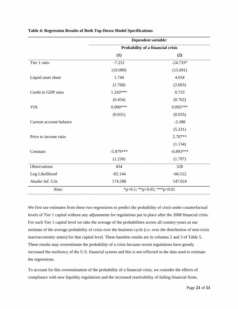
Table 4: Regression Results of Both Top-Down Model Specifications
Dependent variable:
Probability of a financial crisis
(1) (2)
Tier 1 ratio -7.251
(10.089)
-24.733*
(15.691)
Liquid asset share 1.744
(1.768)
4.034
(2.603)
Credit to GDP ratio 1.243***
(0.454)
0.733
(0.702)
VIX 0.090***
(0.031)
0.095***
(0.035)
Current account balance -3.388
(5.231)
Price to income ratio 2.707**
(1.134)
Constant -5.879***
(1.230)
-6.893***
(1.797)
Observations 434 328
Log Likelihood -82.144 -66.512
Akaike Inf. Crit. 174.288 147.024
Note: *p<0.1; **p<0.05; ***p<0.01
We first use estimates from these two regressions to predict the probability of crisis under counterfactual
levels of Tier 1 capital without any adjustments for regulations put in place after the 2008 financial crisis.
For each Tier 1 capital level we take the average of the probabilities across all country-years as our
estimate of the average probability of crisis over the business cycle (i.e. over the distribution of non-crisis
macroeconomic states) for that capital level. These baseline results are in columns 2 and 3 of Table 5.
These results may overestimate the probability of a crisis because recent regulations have greatly
increased the resiliency of the U.S. financial system and this is not reflected in the data used to estimate
the regressions.
To account for this overestimation of the probability of a financial crisis, we consider the effects of
compliance with new liquidity regulations and the increased resolvability of failing financial firms.

Page 22 of 51
Liquidity regulations, particularly the LCR requirement, would be best captured by our share of liquid
asset variable. As shown in
Table 4, the estimated coefficient for this variable is positive but insignificant in both specifications of our
model. For this reason accounting for liquidity regulation compliance would not significantly alter the
results of the top-down method and we do not perform an adjustment for liquidity regulation.
We next consider the effect of increased resolvability of failing financial firms. As described in the
Institutional Environment section, new resolution regulations such as TLAC create a source of funding
for recapitalization that is not directly reflected in either specification of our model. Therefore we follow
the adjustment method of the bottom-up approach and assume a 30 percent reduction in the probability of
a crisis as a result of the increased resolvability of firms. Results reflecting this reduction are shown in the
final two columns of Table 5. These results are most representative of the probability of a crisis in the
current regulatory environment.
Table 5 provides the results of the top-down method. The first column shows various counterfactual
levels of the Tier 1 capital ratio. The next two columns show probabilities of crisis resulting from both
specifications of the model with no adjustment for increased resolvability or liquidity regulations. The last
two columns consider the effect of increased resolvability.
Table 5: Results of the Top-Down Approach
Annual probability of financial crisis (percent)
No adjustments Adjustment for increased resolvability
Tier 1 capital ratio
Specification (1)
Specification (2)
Specification (1)
Specification (2)
8.0 6.3 6.8 4.4 4.7 11.0 5.2 3.3 3.6 2.3 14.0 4.3 1.5 3.0 1.1 17.0 3.5 0.7 2.5 0.5 21.0 2.7 0.2 1.9 0.2 25.0 2.0 0.1 1.4 0.1
The differences between the two specifications show that the relatively limited number of financial crises
mean that results can be sensitive to the sample selection and choice of macroeconomic control variables.
As in the bottom-up method, both specifications of the model attribute higher Tier 1 capital ratios with
lower probabilities of crisis. However, specification (2) shows far greater sensitivity of probabilities to
Page 23 of 51
capital ratios and produces estimates more similar to those of the bottom-up method. In this case, most of
this difference is driven by differences between the data sample used in the two specifications.
Our top-down approach is very similar to that taken by The Bank of England (2015). The Laeven and
Valencia (2012) definition of a systemic banking crisis is used in both studies. The Bank of England
considers one specification of their logit model which differs from our specification (1) only in that it
includes total deposits to total liabilities as an additional explanatory variable. This variable is also
included as a control in the BCBS LEI (2010). While total deposits to total liabilities is a useful variable
for distinguishing between asset and liability liquidity, we were unable to include it in our analysis for
data availability reasons. Table 6 offers a comparison between our top-down results and those of The
Bank of England (2015).
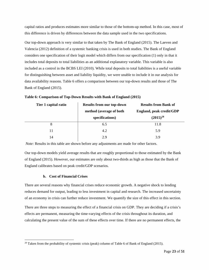
Table 6: Comparison of Top-Down Results with Bank of England (2015)
Tier 1 capital ratio Results from our top-down
method (average of both
specifications)
Results from Bank of
England, peak credit/GDP
(2015)28
8 6.5 11.8
11 4.2 5.9
14 2.9 3.9
Note: Results in this table are shown before any adjustments are made for other factors.
Our top-down models yield average results that are roughly proportional to those estimated by the Bank
of England (2015). However, our estimates are only about two-thirds as high as those that the Bank of
England calibrates based on peak credit/GDP scenarios.
b. Cost of Financial Crises
There are several reasons why financial crises reduce economic growth. A negative shock to lending
reduces demand for output, leading to less investment in capital and research. The increased uncertainty
of an economy in crisis can further reduce investment. We quantify the size of this effect in this section.
There are three steps to measuring the effect of a financial crisis on GDP. They are deciding if a crisis’s
effects are permanent, measuring the time-varying effects of the crisis throughout its duration, and
calculating the present value of the sum of these effects over time. If there are no permanent effects, the
28 Taken from the probability of systemic crisis (peak) column of Table 6 of Bank of England (2015).
Page 24 of 51
cost is simply the present value of the short- and medium-term effects. We discuss each of these steps
below.
Does a Crisis Have Permanent or Persistent Effects?
Measuring the duration of the effects is especially important because it has a large impact on the cost
estimate, even changing the order of magnitude. A permanent effect, even with a high discount rate, will
have a much larger present value than a transitory effect. Some studies assume that a crisis’ duration is
the length of time required for a country to attain the same growth rate in the years prior to the crisis.29 An
example of such a study is Bordo et al. (2001), who analyze financial crises in a variety of countries on
120 years of data.30 They find the duration is quite short, an average of two-and-a-half years for crises
occurring between 1973 and 1997.
A shortcoming of such studies is that they ignore performance of the economy after one period of prior
trend growth. If the economy achieves high growth for one period, and then growth falls below the pre-
crisis trend again and generally stays there, such approaches would state that there is no permanent effect.
They also rule out permanent effects by construction.
Other studies leave the duration of a crises’ effects open as an empirical question, and generally find
support for long lasting effects. Furceri and Mourougane (2012), analyze OECD countries and compare
actual output after a crisis with a measure of potential input. They estimate autoregressive equations and
the implied impulse response functions, finding an average permanent reduction in GDP of 2 percent.
Cerra and Saxena (2008), analyzing data from over 120 countries, find evidence that effects of a financial
crisis on GDP are barely reduced by one percentage point after ten years, remaining at a level of six
percent. These studies provide evidence for robust long-lasting effects. We assume that financial crises
have persistent effects in the rest of the analysis.
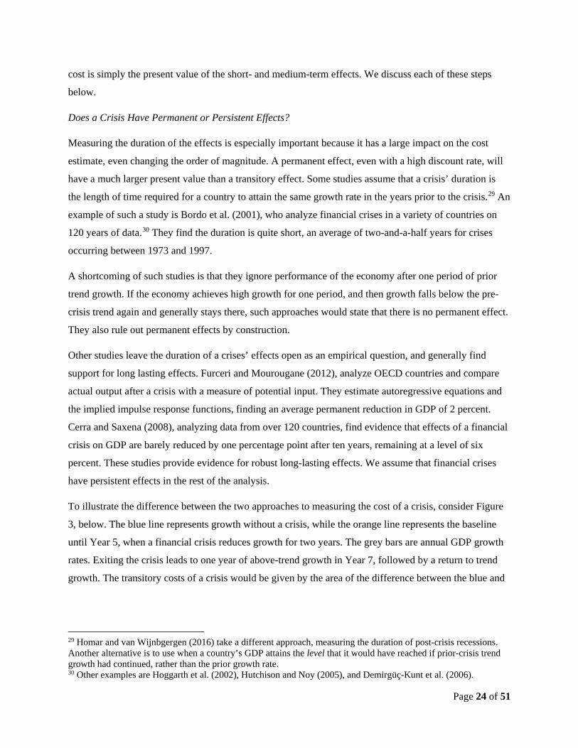
To illustrate the difference between the two approaches to measuring the cost of a crisis, consider Figure
3, below. The blue line represents growth without a crisis, while the orange line represents the baseline
until Year 5, when a financial crisis reduces growth for two years. The grey bars are annual GDP growth
rates. Exiting the crisis leads to one year of above-trend growth in Year 7, followed by a return to trend
growth. The transitory costs of a crisis would be given by the area of the difference between the blue and
29 Homar and van Wijnbgergen (2016) take a different approach, measuring the duration of post-crisis recessions. Another alternative is to use when a country’s GDP attains the level that it would have reached if prior-crisis trend growth had continued, rather than the prior growth rate. 30 Other examples are Hoggarth et al. (2002), Hutchison and Noy (2005), and Demirgüç-Kunt et al. (2006).
Page 25 of 51
orange lines for Years 5 and 6, adjusted for discounting.31 Measuring the permanent effect would include
the area of the discounted difference between the two lines from Year 5 onwards. Of course, if the effects
are not permanent then at some point the blue and orange lines coincide and the effect of the crisis is
reduced to zero as is the area between the two lines beyond that point.
Figure 3: GDP Level (Left Axis) and Growth (Right Axis), Hypothetical Economy
Given the empirical results in Furceri and Mourougane (2012), we think it is sensible to include long-
lasting effects. However, as it is very difficult to statistically distinguish between permanent and highly
persistent effects, we present results using an alternative assumption of a persistent but temporary effect
that fades gradually over time.
Using the Gordon Growth formula, the value of a perpetuity paying once a year is:
𝑃𝑃𝑉𝑉 =𝑑𝑑𝐵𝐵𝐵𝐵𝑅𝑅𝐵𝐵𝐶𝐶 𝐵𝐵𝑁𝑁𝐵𝐵𝑁𝑁𝐵𝐵𝐵𝐵𝑁𝑁
𝐺𝐺𝐵𝐵𝐵𝐵𝑅𝑅𝑜𝑜𝑅𝑅𝐵𝐵𝑁𝑁 𝑅𝑅𝐵𝐵𝑁𝑁𝑁𝑁 − 𝐺𝐺𝑃𝑃𝑜𝑜𝐺𝐺𝑁𝑁ℎ 𝑅𝑅𝐵𝐵𝑁𝑁𝑁𝑁
We can treat the rate of decay as a negative growth rate, yielding:
𝑃𝑃𝑉𝑉 =𝑑𝑑𝐵𝐵𝐵𝐵𝑅𝑅𝐵𝐵𝐶𝐶 𝐵𝐵𝑁𝑁𝐵𝐵𝑁𝑁𝐵𝐵𝐵𝐵𝑁𝑁
𝐺𝐺𝐵𝐵𝐵𝐵𝑅𝑅𝑜𝑜𝑅𝑅𝐵𝐵𝑁𝑁 𝑅𝑅𝐵𝐵𝑁𝑁𝑁𝑁 + 𝑅𝑅𝐵𝐵𝑁𝑁𝑁𝑁 𝑜𝑜𝐵𝐵 𝐺𝐺𝑁𝑁𝑅𝑅𝐵𝐵𝑃𝑃
As this value is as of the beginning of the perpetuity flow, we further discount it back to the beginning of
the crisis. There is no empirical work to our knowledge indicating the proper rate of decay of long-lasting
31 Defining the end of a crisis’ effects as when the economy exits recession would give the same results. If we define the temporary effects as occurring when the economy reaches its pre-crisis growth path, the crisis would end when the two lines intersect.
-0.03
-0.02
-0.01
0
0.01
0.02
0.03
0.04
0.05
100
105
110
115
120
125
130
135
1 2 3 4 5 6 7 8 9 10 11 12 13 14 15
GDP
Grow
th
GDP
Leve
l
Axis Title
GDP Growth Baseline GDP GDP with Crisis
Page 26 of 51
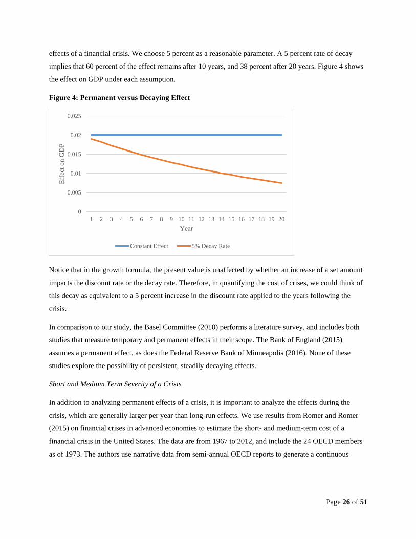
effects of a financial crisis. We choose 5 percent as a reasonable parameter. A 5 percent rate of decay
implies that 60 percent of the effect remains after 10 years, and 38 percent after 20 years. Figure 4 shows
the effect on GDP under each assumption.
Figure 4: Permanent versus Decaying Effect
Notice that in the growth formula, the present value is unaffected by whether an increase of a set amount
impacts the discount rate or the decay rate. Therefore, in quantifying the cost of crises, we could think of
this decay as equivalent to a 5 percent increase in the discount rate applied to the years following the
crisis.
In comparison to our study, the Basel Committee (2010) performs a literature survey, and includes both
studies that measure temporary and permanent effects in their scope. The Bank of England (2015)
assumes a permanent effect, as does the Federal Reserve Bank of Minneapolis (2016). None of these
studies explore the possibility of persistent, steadily decaying effects.
Short and Medium Term Severity of a Crisis
In addition to analyzing permanent effects of a crisis, it is important to analyze the effects during the
crisis, which are generally larger per year than long-run effects. We use results from Romer and Romer
(2015) on financial crises in advanced economies to estimate the short- and medium-term cost of a
financial crisis in the United States. The data are from 1967 to 2012, and include the 24 OECD members
as of 1973. The authors use narrative data from semi-annual OECD reports to generate a continuous
0
0.005
0.01
0.015
0.02
0.025
1 2 3 4 5 6 7 8 9 10 11 12 13 14 15 16 17 18 19 20
Effe
ct o
n G
DP
Year
Constant Effect 5% Decay Rate
Page 27 of 51
measure of the intensity of a crisis, and run a regression with GDP growth, the state of a country’s
financial system, lags of both variables, and other controls.32
There are other studies measuring the overall short and medium term costs of a financial crisis. Examples
include Hoggarth et al. (2002), Hutchison and Noy (2005) and Demirgüç-Kunt at al. (2006). We use
results from Romer and Romer (2015) because they are focused on advanced countries, and thus most
relevant to the United States. Romer and Romer (2015) are also unique in that they provide estimates of
the semi-annual dynamics of the effect on GDP, rather than a single aggregated number. A further
advantage is that they incorporate results from the 2008 financial crisis. The dynamics allow a more
credible analysis of the effects of shortening crises through prompt recapitalization, as discussed below.
Romer and Romer (2015) present estimates of the effect on GDP using a standard, ordinary least squares
(OLS) regression, which weights each observation equally. They also present estimates using a
statistically superior generalized least squares (GLS) approach, which provides less weight to
observations from countries with a high variance of GDP growth. Most of these high variance countries
are smaller or less economically advanced. For example, the variance of GDP in Turkey, Iceland, and
Ireland is much larger than the United States or other advanced countries (see Figure 5). Such countries’
economies are more influenced by international capital markets and/or sovereign risk. Nonetheless, data
on financial crises are limited, and it is useful to include these countries in the analysis. As a compromise,
we focus on Romer and Romer’s GLS estimates, as they provide less weight to these high-variance
countries that are arguably less comparable to the United States.
32 Note that our analysis of the probability of a crisis uses the definition in Laeven and Valencia (2012). See section I.D of Romer and Romer (2015) for a comparison of the financial crises identified by their method and an updated version of the data used by Laeven and Valencia (2012). The two are almost identical. Furceri and Mourougane (2012) use the same definition as Laeven and Valencia (2012).

Page 28 of 51
Figure 5: Standard Deviation of Quarterly GDP Growth by Country
Source: Analysis of OECD data, https://data.oecd.org/gdp/quarterly-gdp.htm#indicator-chart. Standard deviation of annualized quarterly growth rates, 2001:Q1–2015:Q3. Note 2016:Q3 data for Luxembourg, New Zealand, and Turkey are not yet available. Sample is OECD early members.
The authors give estimates of the reduction in GDP due to financial crises in advanced economies on a
semi-annual basis over five years. Their results with both GLS and OLS are shown below in Table 7.33
Table 7: Short-to-Medium Effects of Financial Crisis per Half Year % of GDP, From Romer and Romer (2015)
Time Lag Max Response Specification 0 2.5 Years 5 Years
OLS -2.08 -4.72 -4.61 -5.96 GLS -1.24 -3.26 -2.25 -4.07
Source: Romer and Romer (2015), Table 2
Both specifications show that a relatively small effect, which is contemporaneous with the crisis, becomes
larger in magnitude and reaches a peak after two-and-a-half years, afterwards slowly becoming smaller.
Present Value Calculation
We use a linear interpolation of Romer and Romer’s (2015) GLS results for the effect of a financial crisis
up to five years and assume a permanent reduction in GDP as found by Furceri and Mourougane (2012)
33 These numbers are calibrated to represent a “moderate” crisis. The last time they designate the United States as having been in such a crisis state was the second half of 2009.
0.000.020.040.060.080.100.120.140.160.18
Aus
tralia
Fran
ceB
elgi
umSw
itzer
land
Uni
ted
Stat
esC
anad
aU
nite
d K
ingd
omN
ew Z
eala
ndIta
lyN
ethe
rland
sSp
ain
Aus
tria
Portu
gal
Ger
man
yD
enm
ark
Swed
enJa
pan
Nor
way
Finl
and
Gre
ece
Luxe
mbo
urg
Turk
eyIc
elan
dIr
elan
d
Stan
dard
Dev
iatio
n of
GD
P G
row
th
Country

Page 29 of 51
of 2 percent afterwards. We also calculate the impact of an effect whose magnitude decays 5 percent a
year. In order to turn these estimates into a net present value, we need to apply a discount rate to the
future reductions in GDP. Standard asset pricing models imply that the real risk-free rate reflects the
intertemporal preferences for the economy. We use the average real yield on 10 year Treasury bonds, or
2.7 percent.34 Table 8 shows the estimated present value of the cost of a financial crisis, under our two
assumptions about the permanence of effects. As discussed below, we adjust these results for the effects
of prompt recapitalization requirements and the increased resolvability of failing financial firms. The
magnitude of the effect is quite sensitive to assumptions about decay (or discount) rates, falling by more
than half if we assume a 5 percent rate of decay.
Table 8: Estimated Cost of a Financial Crisis, Unadjusted for Increased Resolvability
Rate of Decay Estimated Cost (percent of GDP)
0 percent 103 percent 5 percent 44 percent
Improved resolvability requirements, discussed above, likely will cause future recapitalizations to happen
more rapidly than is typical for advanced countries in the past. Research suggests that prompt
recapitalization reduces the duration of financial crises. Homar and van Wijnbgergen (2016) conclude that
with prompt recapitalizations, the time to a GDP trough is two years, rather than three-and-a-half years,
and the duration of effects is three years, rather than five. We maintain the Romer and Romer (2015)
estimates of the peak and final semi-annual costs of a financial crisis and calculate the revised costs given
the shorter duration. Figure 6 shows the estimated semi-annual cost under this assumption.
34 We use all monthly data from 1962 to 2006, and calculate inflation from the CPI for all urban consumers. We stop at 2006 because the subsequent period represents an extreme in monetary policy. Data were obtained from the Federal Reserve Bank of St. Louis Economic Research web-site at https://research.stlouisfed.org/.
Page 30 of 51
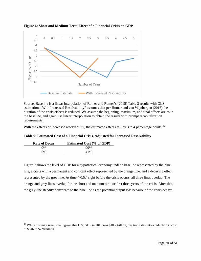
Figure 6: Short and Medium Term Effect of a Financial Crisis on GDP
Source: Baseline is a linear interpolation of Romer and Romer’s (2015) Table 2 results with GLS estimation. “With Increased Resolvability” assumes that per Homar and van Wijnbergen (2016) the duration of the crisis effects is reduced. We assume the beginning, maximum, and final effects are as in the baseline, and again use linear interpolation to obtain the results with prompt recapitalization requirements.
With the effects of increased resolvability, the estimated effects fall by 3 to 4 percentage points.35
Table 9: Estimated Cost of a Financial Crisis, Adjusted for Increased Resolvability
Rate of Decay Estimated Cost (% of GDP) 0% 99% 5% 41%
Figure 7 shows the level of GDP for a hypothetical economy under a baseline represented by the blue
line, a crisis with a permanent and constant effect represented by the orange line, and a decaying effect
represented by the grey line. At time “-0.5,” right before the crisis occurs, all three lines overlap. The
orange and grey lines overlap for the short and medium term or first three years of the crisis. After that,
the grey line steadily converges to the blue line as the potential output loss because of the crisis decays.
35 While this may seem small, given that U.S. GDP in 2015 was $18.2 trillion, this translates into a reduction in cost of $546 to $728 billion.
-4.5
-4
-3.5
-3
-2.5
-2
-1.5
-1
-0.5
00 0.5 1 1.5 2 2.5 3 3.5 4 4.5 5
Effe
ct a
s % o
f GD
P
Number of Years
Baseline Estimate With Increased Resolvability

Page 31 of 51
Figure 7: Level of GDP, No Crisis, Crisis with Permanent Constant Effects, and Crisis with Decaying Effects
For the sake of comparison, the Basel Committee (2010) report, as shown below, reports the average cost
of a financial crisis ranges from 19 percent to 158 percent depending whether the effects are permanent.
Their results are based on a meta-analysis of other studies, and do not focus on advanced economies.
Their low estimates include several studies that assume no permanent effect. The Federal Reserve Bank
of Minneapolis (2016) adopts the high estimate of 158 percent from the Basel Committee report.
The Bank of England (2015) estimates a 43 percent cost for the UK, based on the Romer and Romer
(2015) OLS methodology, with multiple adjustments. They also assume the effect of a crisis is
permanent. Their adjustments include a different approach to estimating the effects of increased
resolvability that implies a much larger impact. They focus on TLAC in particular and assume that TLAC
will lead to a rapid, credible bail-in which will ensure that any crises will be like the least severe historic
crises, and thus adjust their estimated cost of crisis down by approximately 60 percent. Given that there
has not yet been a TLAC “bail-in” and that there are multiple differences between the U.S. economy and
many economies in their sample of “less severe” crises, we opt for a more conservative approach to
measuring the effects of increased resolvability. Other studies’ results are summarized in Table 10.
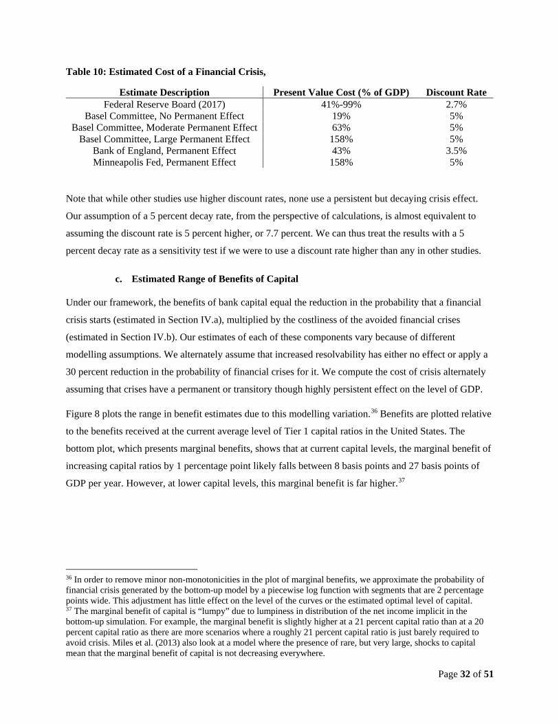
Page 32 of 51
Table 10: Estimated Cost of a Financial Crisis,
Estimate Description Present Value Cost (% of GDP) Discount Rate Federal Reserve Board (2017) 41%-99% 2.7%
Basel Committee, No Permanent Effect 19% 5% Basel Committee, Moderate Permanent Effect 63% 5%
Basel Committee, Large Permanent Effect 158% 5% Bank of England, Permanent Effect 43% 3.5% Minneapolis Fed, Permanent Effect 158% 5%
Note that while other studies use higher discount rates, none use a persistent but decaying crisis effect.
Our assumption of a 5 percent decay rate, from the perspective of calculations, is almost equivalent to
assuming the discount rate is 5 percent higher, or 7.7 percent. We can thus treat the results with a 5
percent decay rate as a sensitivity test if we were to use a discount rate higher than any in other studies.
c. Estimated Range of Benefits of Capital
Under our framework, the benefits of bank capital equal the reduction in the probability that a financial
crisis starts (estimated in Section IV.a), multiplied by the costliness of the avoided financial crises
(estimated in Section IV.b). Our estimates of each of these components vary because of different
modelling assumptions. We alternately assume that increased resolvability has either no effect or apply a
30 percent reduction in the probability of financial crises for it. We compute the cost of crisis alternately
assuming that crises have a permanent or transitory though highly persistent effect on the level of GDP.
Figure 8 plots the range in benefit estimates due to this modelling variation.36 Benefits are plotted relative
to the benefits received at the current average level of Tier 1 capital ratios in the United States. The
bottom plot, which presents marginal benefits, shows that at current capital levels, the marginal benefit of
increasing capital ratios by 1 percentage point likely falls between 8 basis points and 27 basis points of
GDP per year. However, at lower capital levels, this marginal benefit is far higher.37
36 In order to remove minor non-monotonicities in the plot of marginal benefits, we approximate the probability of financial crisis generated by the bottom-up model by a piecewise log function with segments that are 2 percentage points wide. This adjustment has little effect on the level of the curves or the estimated optimal level of capital. 37 The marginal benefit of capital is “lumpy” due to lumpiness in distribution of the net income implicit in the bottom-up simulation. For example, the marginal benefit is slightly higher at a 21 percent capital ratio than at a 20 percent capital ratio as there are more scenarios where a roughly 21 percent capital ratio is just barely required to avoid crisis. Miles et al. (2013) also look at a model where the presence of rare, but very large, shocks to capital mean that the marginal benefit of capital is not decreasing everywhere.
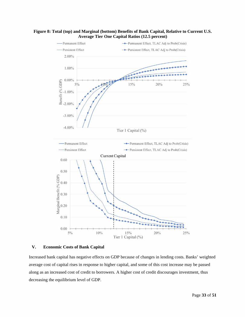
Page 33 of 51
Figure 8: Total (top) and Marginal (bottom) Benefits of Bank Capital, Relative to Current U.S. Average Tier One Capital Ratios (12.5 percent)
V. Economic Costs of Bank Capital
Increased bank capital has negative effects on GDP because of changes in lending costs. Banks’ weighted
average cost of capital rises in response to higher capital, and some of this cost increase may be passed
along as an increased cost of credit to borrowers. A higher cost of credit discourages investment, thus
decreasing the equilibrium level of GDP.

Page 34 of 51
The first step in estimating the impact of bank capital on the level of GDP is to estimate how changes in
capital affect the cost of loans. To do this, we estimate the impact of capital on a representative bank’s
weighted average cost of capital. Next, we calculate how much loan rates would have to change in order
to offset these changes to the cost of capital. We alternately assume that banks are able to pass on 50
percent or 100 percent of these changes in the form of increased lending costs.
Once we have estimated the impact of capital on lending costs, we use the FRB/US macroeconomic
model to assess the effect of these changes in lending costs on the equilibrium level of GDP.38 The
FRB/US macroeconomic model is a large-scale macro model used by Federal Reserve staff to track the
evolution of the U.S. economy over time. The model is well documented and versions of it are freely
available to the public.39 It is used here as a baseline economic model to translate increased lending
spreads into reduced GDP levels and follows previous work conducted by the Federal Reserve Bank of
Minneapolis (2016).
Bank Capital Structure and the Modigliani-Miller Theorem
Bank equity is a residual claim on the bank’s income and assets, therefore requiring a higher return than
debt. One might think that increased capital would thus require a higher return on assets in order to fund
these higher returns on part of the capital structure. However, the Modigliani-Miller Theorem implies no
such effects, as decreased leverage reduces risk and results in decreased required rates of return on equity
and debt. The extent to which the Theorem applies to U.S. banks is not clear, as discussed below. The
relevance of Modigliani-Miller for banks is controversial, and has important implications for our findings.
Notable papers arguing that the theorem applies to banks include Miller (1995) and Admati et al. (2014).
There are reasons, even in the presence of full Modigliani-Miller effects, that banks may need to increase
their return on assets due to an increase in capital. These are discussed in Elliott (2013), among other
places. The Modigliani-Miller Theorem assumes that capital structure has no effect on taxes. Interest
payments on debt are tax-deductible while dividends are not, so higher equity means that banks lose some
of the tax advantages of high debt levels.
Ultimately, whether the theorem applies or not is an empirical question. A common approach is to
consider the effects of changes in bank capital structure on bank equity covariance with the market, or
“beta.” According to finance theory, market betas determine the required return on assets. If market beta
38 We thank Michael Siemer for using FRB/US to calculate the effect of an increase in lending costs on the level of GDP. 39 For more information on the FRB/US model see the Federal Reserve Board’s website at www.federalreserve.gov/econresdata/notes/feds-notes/2014/a-tool-for-macroeconomic-policy-analysis.html.
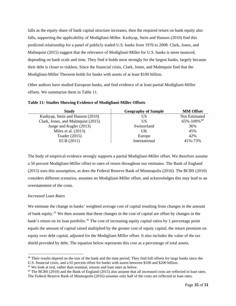
Page 35 of 51
falls as the equity share of bank capital structure increases, then the required return on bank equity also
falls, supporting the applicability of Modigliani-Miller. Kashyap, Stein and Hanson (2010) find this
predicted relationship for a panel of publicly traded U.S. banks from 1976 to 2008. Clark, Jones, and
Malmquist (2015) suggest that the relevance of Modigliani-Miller for U.S. banks is more nuanced,
depending on bank scale and time. They find it holds most strongly for the largest banks, largely because
their debt is closer to riskless. Since the financial crisis, Clark, Jones, and Malmquist find that the
Modigliani-Miller Theorem holds for banks with assets of at least $100 billion.
Other authors have studied European banks, and find evidence of at least partial Modigliani-Miller
offsets. We summarize them in Table 11.
Table 11: Studies Showing Evidence of Modigliani-Miller Offsets
Study Geography of Sample MM Offset Kashyap, Stein and Hanson (2010) US Not Estimated Clark, Jones, and Malmquist (2015) US 65%-100%40
Junge and Kugler (2013) Switzerland 36% Miles et al. (2013) UK 45%
Toader (2015) Europe 42% ECB (2011) International 41%-73%
The body of empirical evidence strongly supports a partial Modigliani-Miller offset. We therefore assume
a 50 percent Modigliani-Miller offset to rates of return throughout our estimates. The Bank of England
(2015) uses this assumption, as does the Federal Reserve Bank of Minneapolis (2016). The BCBS (2010)
considers different scenarios, assumes no Modigliani-Miller offset, and acknowledges this may lead to an
overstatement of the costs.
Increased Loan Rates
We estimate the change in banks’ weighted average cost of capital resulting from changes in the amount
of bank equity.41 We then assume that these changes in the cost of capital are offset by changes in the
bank’s return on its loan portfolio.42 The cost of increasing equity capital ratios by 1 percentage point
equals the amount of capital raised multiplied by the greater cost of equity capital, the return premium on
equity over debt capital, adjusted for the Modigliani-Miller offset. It also includes the value of the tax
shield provided by debt. The equation below represents this cost as a percentage of total assets.
40 Their results depend on the size of the bank and the time period. They find full offsets for large banks since the U.S. financial crisis, and a 65 percent offset for banks with assets between $100 and $200 billion. 41 We look at real, rather than nominal, returns and loan rates as below. 42 The BCBS (2010) and the Bank of England (2015) also assume that all increased costs are reflected in loan rates. The Federal Reserve Bank of Minneapolis (2016) assumes only half of the costs are reflected in loan rates.

Page 36 of 51
0.01 ∗ 𝑅𝑅𝑅𝑅𝐴𝐴𝐴𝐴𝐴𝐴𝐴𝐴𝐴𝐴𝑡𝑡𝐴𝐴
∗ [(1 −𝑀𝑀𝑀𝑀) ∗ (𝑅𝑅𝐸𝐸 − 𝑅𝑅𝐷𝐷) + 𝑅𝑅𝐷𝐷 ∗ 𝑁𝑁]
RE is the return on equity, RD is the return on debt, MM is the degree of the Modigliani-Miller offset, and t
is the corporate tax rate.
For the average risk weight, RWA/assets, we use the asset-weighted average for large U.S. banks as of
the end of 2015, which is 66 percent.43 Substituting, this becomes:
0.01 ∗ 66% ∗ [(1 −𝑀𝑀𝑀𝑀) ∗ (𝑅𝑅𝐸𝐸 − 𝑅𝑅𝐷𝐷) + 𝑅𝑅𝐷𝐷 ∗ 𝑁𝑁]
To estimate the return on bank debt, RD, we look at the past fifteen years. We consider annual data on all
U.S. top-tier bank holding companies with assets of at least $50 billion in 2015 dollars. During the past 15
years, median interest costs were 1.61 percent on average. However, we consider recent very low interest
rates to be a historic abnormality, so we use the pre-crisis (2001 through 2006) period, for which median
interest costs averaged 2.32 percent.44 Thus we find:
0.01 ∗ 66% ∗ [(1 −𝑀𝑀𝑀𝑀) ∗ (𝑅𝑅𝐸𝐸 − 2.32%) + 2.32% ∗ 𝑁𝑁]
In order to estimate the return on bank equity, RE, we apply the capital asset pricing model (CAPM).
Under the CAPM, the expected return on bank equity is equal to the risk free rate, Rf, plus a premium
equal to bank equity’s comovement with the market (given by beta) multiplied by the expected return on
the market RM in excess of the risk-free rate:
𝑅𝑅𝐸𝐸 = 𝑅𝑅𝑓𝑓 + 𝛽𝛽 ∗ (𝑅𝑅𝑀𝑀 − 𝑅𝑅𝑓𝑓)
With 15 years of data, we calibrate the model to an average risk-free rate of 2.32 percent and average
excess market returns of 5.24 percent. We estimate a daily beta of 1.35 for the domestic U.S. top-tier
holding companies, based on data from 2010 to 2015, implying an expected return for bank equity of 8.71
percent.45 To complete the estimate, we use a corporate tax rate, t, of 43.7 percent.46
43 Many recent changes have affected banks’ asset composition and RWA calculations in recent years, including the implementation of Basel III, the Volcker rule, and liquidity and TLAC regulations. Therefore we use data on both RWA/assets, assets/loans, and interest expense from December 2015, the most recent full year for which data are available. Neither the interest rate environment nor regulations governing RWA calculations have changed since then in a way that would significantly affect our conclusions. 44 Kayshap, Stein, and Hanson (2010) assume that additional equity will displace either long-term or short-term debt. TLAC and liquidity requirements mean that banks are now less free to adjust their liability composition. Thus, we use the average liability cost. 45 We use data starting in 2010 for calculating beta because the large number of mergers and acquisitions following the crisis would muddy the analysis prior to that date. 46 We follow Clark, Jones and Malmquist (2015) in assuming a Delaware residence. Delaware has a tax rate of 8.37 percent, and the federal corporate tax rate is 35 percent. Only South Dakota and Wyoming have no corporate income
Page 37 of 51
This implies
0.01 ∗ 66% ∗ [(1 −𝑀𝑀𝑀𝑀) ∗ (8.71% − 2.32%) + 2.32% ∗ 43.7%]
We assume that half of the Modigliani-Miller offset occurs
0.01 ∗ 66% ∗ [0.5 ∗ (8.71% − 2.32%) + 2.32% ∗ 43.7%]
We thus project an increase in asset return rates of 2.7 basis points per 1 percentage point increase in
capital ratios, of which 0.7 basis points is attributed to the debt shield.
We assume this increase in cost is passed along entirely in the form of increased rates on loans. As loans
currently comprise about 40 percent of bank assets, we divide the increase in cost of capital by 40 percent
for our estimate of the increase in loan costs, arriving at 0.00027/0.4 or 6.9 basis points.
There are also reasons to think that banks may not be able to pass along 100 percent of any increased
capital cost to borrowers. Competition with non-bank lenders, and the public debt markets may make it
difficult for banks to pass along increases in the cost of capital. Even without such competition, banks
might increase revenue by reducing the cost of operations, decreasing interest expense, or finding revenue
increases from business lines other than lending.47
We consequently also calculate the effect if banks could only pass through half of their increased cost to
borrowers, implying an increase in loan costs of 3.4 basis points per percentage point increase in equity
capital.48
For the purposes of comparison, the BCBS (2010) study ignores Modigliani-Miller effects in an estimate,
and thus finds a larger increase in lending costs of 13 basis points per percentage point increase in capital
ratios. The Bank of England (2015) estimates an effect of 10 basis points, partially due to the higher bank
equity premium (RE - RD) of 10 percent compared to the United States of 8.71 percent minus 2.32 percent
or 6.39 percent.
or gross receipts tax. State corporate income taxes range from 4 percent to 12 percent for 2016. See http://taxfoundation.org/article/state-corporate-income-tax-rates-and-brackets-2016. 47 Phillipon and Reshef (2012) show that wages in the financial sector from 1990 forwards earned a premiu.m over other sectors. This premium grew over time and cannot be fully explained by risk or technological change. This research suggests that cost reductions are feasible. 48 If only half of the increased cost is passed along in the form of higher loan rates, banks might respond to increased costs in other ways, such as focusing more on higher-yield, and thus risky, lending. Banks might also raise fees for other services in a manner that could create distortions. To our knowledge, there is no adequate empirical basis for modeling such effects.
Page 38 of 51
Translating Loan Rates into GDP
We use the FRB/US model to translate increases in lending rates into a long-run effect on the level of
GDP. FRB/US is a large-scale model of the U.S. economy featuring optimizing behavior by households
and firms as well as detailed descriptions of monetary policy and the fiscal sector. FRB/US has a
neoclassical core that combines a production function with endogenous and exogenous supplies of
production factors and key aspects of household preferences such as impatience. To account for cyclical
fluctuations, the model features rigidities that apply to many decisions made by households and firms.
The model does not explicitly include corporate loan spreads. Therefore, we use the spreads on corporate
bonds to model a shock to corporate lending rates, and spreads on home mortgages and auto loans to
model a shock to consumer lending rates.49
The model predicts that the effects on the equilibrium level of GDP from an increase in lending rates are
approximately linear. A 1 basis point increase in lending rates implies a decrease in the level of GDP of
approximately 1.07 basis points. 50 We estimate the effect of a 1 percentage point increase in capital ratios
is a reduction in the level of long-run GDP of 7.4 basis points. If only half of the cost is passed through in
the form of higher rates on loans, the effect on long-run GDP is 3.7 basis points.
Figure 9 plots these alternative costs of bank capital. The left-hand plot shows total costs increasing
linearly with the capital level, and the right-hand plot shows that this equates to a constant marginal cost
of capital.
49 Most of the effect on GDP is from an increase in corporate lending rates. To the extent that rate increases are limited to other loans, we may be overstating the effects. 50 This is slightly different than the results calculated by the Federal Reserve Bank of Minneapolis (2016). The Federal Reserve Bank of Minneapolis (2016) calculates changes from a long-run baseline, while we use the present-day scenario.
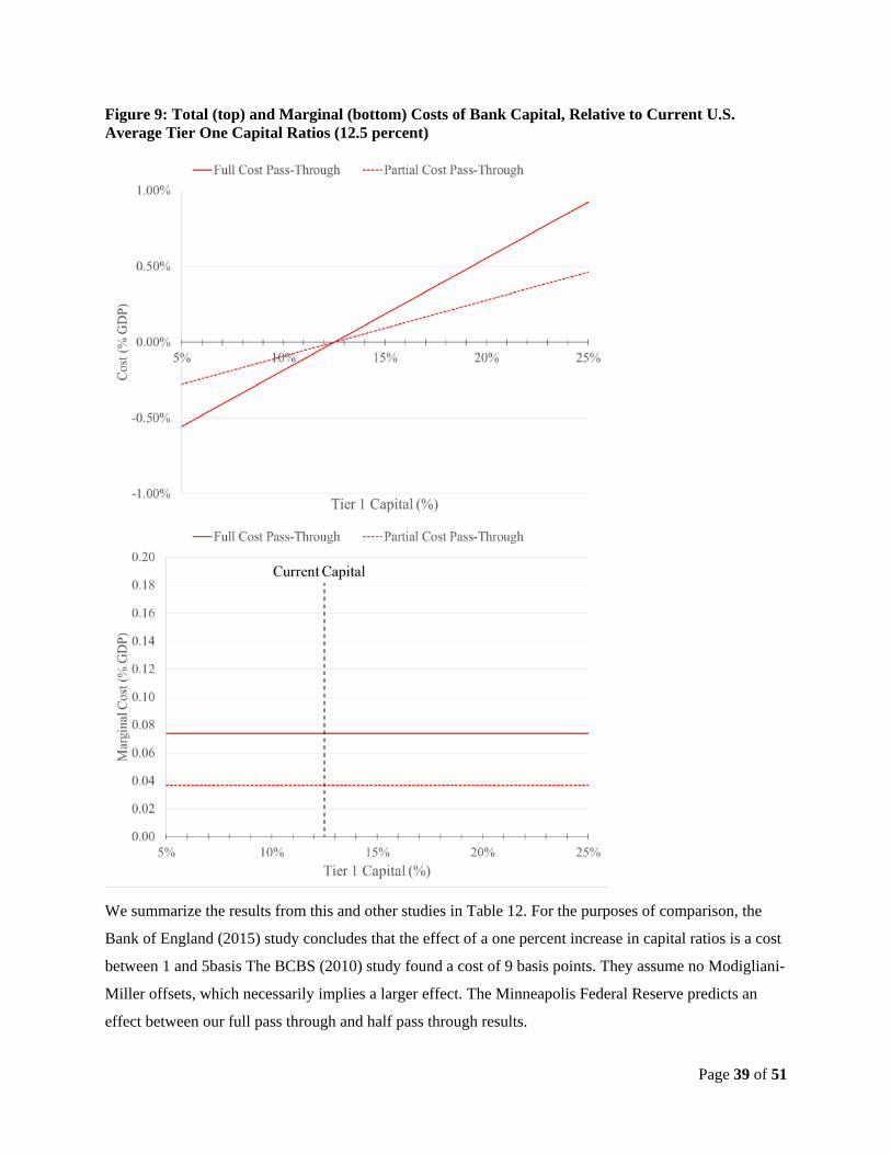
Page 39 of 51
Figure 9: Total (top) and Marginal (bottom) Costs of Bank Capital, Relative to Current U.S. Average Tier One Capital Ratios (12.5 percent)
We summarize the results from this and other studies in Table 12. For the purposes of comparison, the
Bank of England (2015) study concludes that the effect of a one percent increase in capital ratios is a cost
between 1 and 5basis The BCBS (2010) study found a cost of 9 basis points. They assume no Modigliani-
Miller offsets, which necessarily implies a larger effect. The Minneapolis Federal Reserve predicts an
effect between our full pass through and half pass through results.
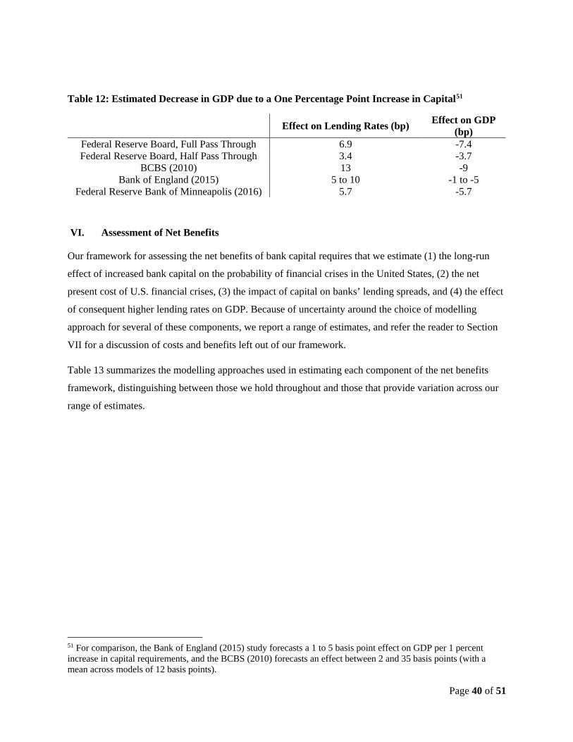
Page 40 of 51
Table 12: Estimated Decrease in GDP due to a One Percentage Point Increase in Capital51
Effect on Lending Rates (bp) Effect on GDP (bp)
Federal Reserve Board, Full Pass Through 6.9 -7.4 Federal Reserve Board, Half Pass Through 3.4 -3.7
BCBS (2010) 13 -9 Bank of England (2015) 5 to 10 -1 to -5
Federal Reserve Bank of Minneapolis (2016) 5.7 -5.7
VI. Assessment of Net Benefits
Our framework for assessing the net benefits of bank capital requires that we estimate (1) the long-run
effect of increased bank capital on the probability of financial crises in the United States, (2) the net
present cost of U.S. financial crises, (3) the impact of capital on banks’ lending spreads, and (4) the effect
of consequent higher lending rates on GDP. Because of uncertainty around the choice of modelling
approach for several of these components, we report a range of estimates, and refer the reader to Section
VII for a discussion of costs and benefits left out of our framework.
Table 13 summarizes the modelling approaches used in estimating each component of the net benefits
framework, distinguishing between those we hold throughout and those that provide variation across our
range of estimates.
51 For comparison, the Bank of England (2015) study forecasts a 1 to 5 basis point effect on GDP per 1 percent increase in capital requirements, and the BCBS (2010) forecasts an effect between 2 and 35 basis points (with a mean across models of 12 basis points).

Page 41 of 51
Table 13: Modeling Assumptions
Key modelling approaches
used in all of our estimates
Sources of variation within
our estimates
Impact of capital on the
probability of crises (accounting
for liquidity regulations)
-use the average of bottom-up
and top-down approaches
-whether increased
resolvability has an impact on
the probability of crisis
Cost of crises (accounting for
enhanced resolvability)
-crises have a long-lasting
effect on the level of GDP
-whether crises have a
permanent constant or
decaying effect on GDP
Impact of capital on bank lending
spreads
-half of the Modigliani Miller
offset applies to impact on the
cost of capital
-extent to which changes in
the cost of capital impact
lending spreads
Impact of bank lending spreads on
GDP
-estimated via model
(FRB/US)
The modelling decisions we make fall within the variation seen in other impact analyses.
We use the average of multiple distinct approaches to estimate the probability of financial crises, as is
also done by the BCBS and Bank of England, though we include a (small) adjustment for U.S. liquidity
regulations. The Bank of England study assumes enhanced resolvability (TLAC) reduces the probability
of crises by 30 percent, but because of uncertainty over the magnitude of this effect, we present estimates
both with and without this adjustment.
When estimating the cost of financial crises, we recognize that it is empirically very difficult to discern
between permanent and highly persistent but temporary effects on GDP. Therefore, we produce estimates
alternately assuming that crises have a permanent effect on the level of GDP (as in the Bank of England,
Minneapolis Fed, and certain of the BCBS estimates), or merely persistent effects. Equivalently, we
estimate the cost assuming permanent effects, but applying a much higher discount rate. As with the Bank
of England analysis, we include an adjustment for increased resolvability, shortening the period of time
where crises have a temporarily large effect on GDP. In our analysis, this adjustment has a relatively
small effect on the overall cost of crisis, as the large long-run cost is unaffected. The Bank of England’s
far larger 60 percent reduction for TLAC is based on the difference in cost of crises sorted by whether
they occurred under more or less credible orderly resolution regimes.
Page 42 of 51
On the cost side, we assume that as banks de-lever, required rates of return on their equity and debt
decline by only half as much as would be implied by the Modigliani Miller theorem adjusted for tax
shield benefits. This assumption is supported by existing research and is also applied in the Bank of
England and Federal Reserve Bank of Minneapolis studies. We express uncertainty over the extent to
which changes in the cost of capital are passed along to borrowers, and assume that this pass-through is
either 50 percent (as in the Minneapolis study) or 100 percent (as is used as the baseline in other studies).
Like the Minneapolis study, we also use the Federal Reserve’s macroeconomic model (FRB/US) to
convert changes in lending spread into changes in long-run GDP. Other studies rely on a range of reduced
form and semi-structural models.
In Figure 10, we plot the range of economic costs and benefits that we model, relative to the costs and
benefits of the current Tier 1 risk-based capital ratio of 12.5 percent for the average U.S. bank. Our low
estimate of the benefits assumes that financial crises cause only gradually decaying reductions in GDP
and that increased resolvability reduces the probability of crises by 30 percent. Our high estimate of the
benefits assumes the financial crises result in permanent reductions in output and that increased
resolvability affects only the cost, and not the probability, of financial crises. Our low and high estimate
of the costs vary only because of the extent that increases in banks’ cost of capital are passed through to
borrowers.
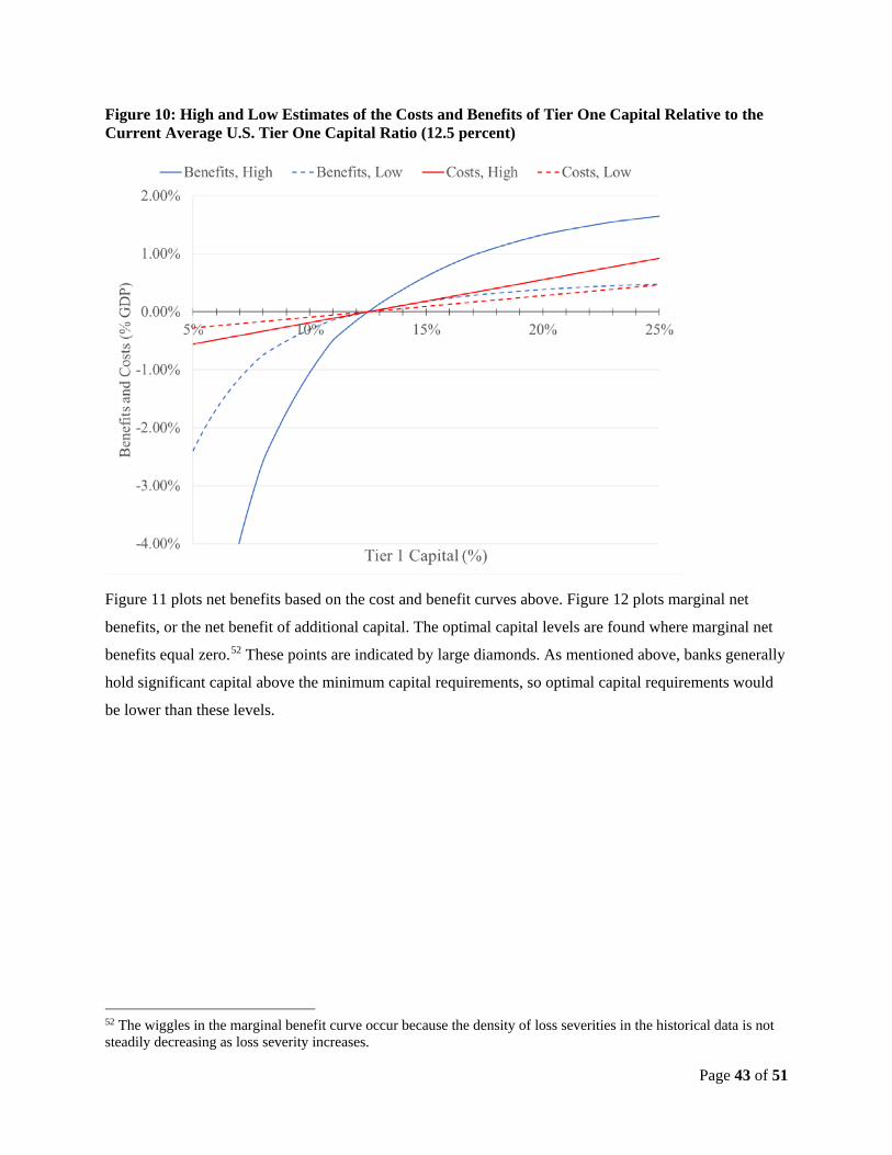
Page 43 of 51
Figure 10: High and Low Estimates of the Costs and Benefits of Tier One Capital Relative to the Current Average U.S. Tier One Capital Ratio (12.5 percent)
Figure 11 plots net benefits based on the cost and benefit curves above. Figure 12 plots marginal net
benefits, or the net benefit of additional capital. The optimal capital levels are found where marginal net
benefits equal zero.52 These points are indicated by large diamonds. As mentioned above, banks generally
hold significant capital above the minimum capital requirements, so optimal capital requirements would
be lower than these levels.
52 The wiggles in the marginal benefit curve occur because the density of loss severities in the historical data is not steadily decreasing as loss severity increases.
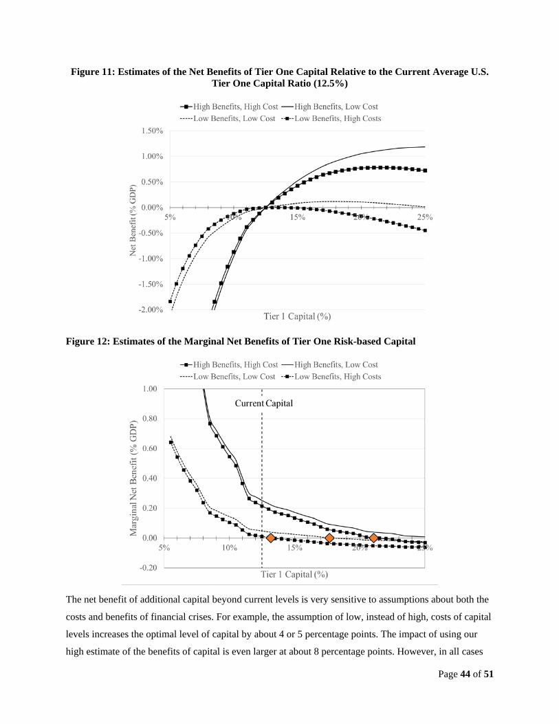
Page 44 of 51
Figure 11: Estimates of the Net Benefits of Tier One Capital Relative to the Current Average U.S. Tier One Capital Ratio (12.5%)
Figure 12: Estimates of the Marginal Net Benefits of Tier One Risk-based Capital
The net benefit of additional capital beyond current levels is very sensitive to assumptions about both the
costs and benefits of financial crises. For example, the assumption of low, instead of high, costs of capital
levels increases the optimal level of capital by about 4 or 5 percentage points. The impact of using our
high estimate of the benefits of capital is even larger at about 8 percentage points. However, in all cases
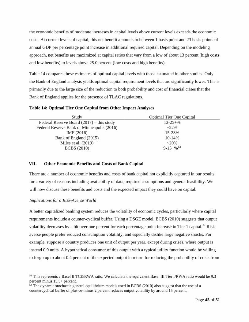
Page 45 of 51
the economic benefits of moderate increases in capital levels above current levels exceeds the economic
costs. At current levels of capital, this net benefit amounts to between 1 basis point and 23 basis points of
annual GDP per percentage point increase in additional required capital. Depending on the modeling
approach, net benefits are maximized at capital ratios that vary from a low of about 13 percent (high costs
and low benefits) to levels above 25.0 percent (low costs and high benefits).
Table 14 compares these estimates of optimal capital levels with those estimated in other studies. Only
the Bank of England analysis yields optimal capital requirement levels that are significantly lower. This is
primarily due to the large size of the reduction to both probability and cost of financial crises that the
Bank of England applies for the presence of TLAC regulations.
Table 14: Optimal Tier One Capital from Other Impact Analyses
Study Optimal Tier One Capital Federal Reserve Board (2017) – this study 13-25+%
Federal Reserve Bank of Minneapolis (2016) ~22% IMF (2016) 15-23%
Bank of England (2015) 10-14% Miles et al. (2013) ~20%
BCBS (2010) 9-15+%53
VII. Other Economic Benefits and Costs of Bank Capital
There are a number of economic benefits and costs of bank capital not explicitly captured in our results
for a variety of reasons including availability of data, required assumptions and general feasibility. We
will now discuss these benefits and costs and the expected impact they could have on capital.
Implications for a Risk-Averse World
A better capitalized banking system reduces the volatility of economic cycles, particularly where capital
requirements include a counter-cyclical buffer. Using a DSGE model, BCBS (2010) suggests that output
volatility decreases by a bit over one percent for each percentage point increase in Tier 1 capital.54 Risk
averse people prefer reduced consumption volatility, and especially dislike large negative shocks. For
example, suppose a country produces one unit of output per year, except during crises, where output is
instead 0.9 units. A hypothetical consumer of this output with a typical utility function would be willing
to forgo up to about 0.4 percent of the expected output in return for reducing the probability of crisis from
53 This represents a Basel II TCE/RWA ratio. We calculate the equivalent Basel III Tier I/RWA ratio would be 9.3 percent minus 15.5+ percent. 54 The dynamic stochastic general equilibrium models used in BCBS (2010) also suggest that the use of a countercyclical buffer of plus-or-minus 2 percent reduces output volatility by around 15 percent.
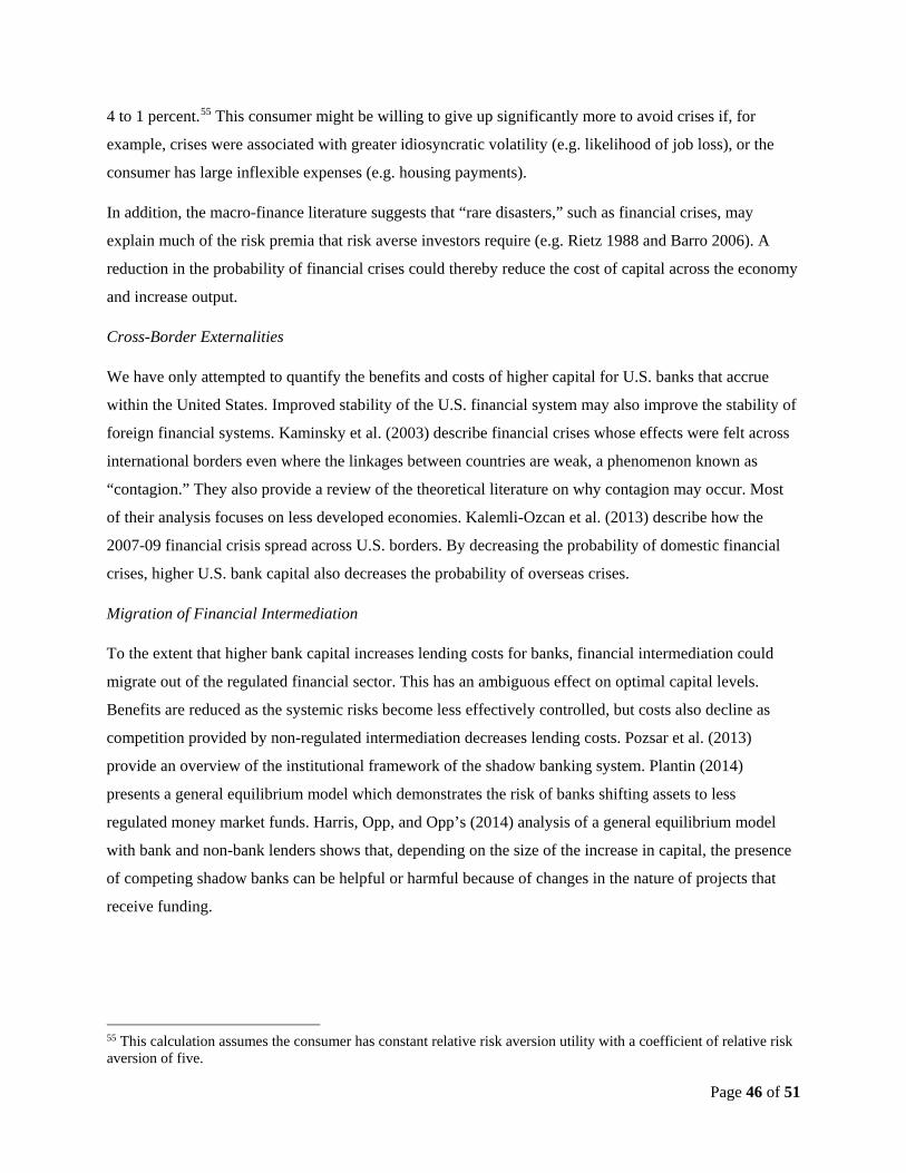
Page 46 of 51
4 to 1 percent.55 This consumer might be willing to give up significantly more to avoid crises if, for
example, crises were associated with greater idiosyncratic volatility (e.g. likelihood of job loss), or the
consumer has large inflexible expenses (e.g. housing payments).
In addition, the macro-finance literature suggests that “rare disasters,” such as financial crises, may
explain much of the risk premia that risk averse investors require (e.g. Rietz 1988 and Barro 2006). A
reduction in the probability of financial crises could thereby reduce the cost of capital across the economy
and increase output.
Cross-Border Externalities
We have only attempted to quantify the benefits and costs of higher capital for U.S. banks that accrue
within the United States. Improved stability of the U.S. financial system may also improve the stability of
foreign financial systems. Kaminsky et al. (2003) describe financial crises whose effects were felt across
international borders even where the linkages between countries are weak, a phenomenon known as
“contagion.” They also provide a review of the theoretical literature on why contagion may occur. Most
of their analysis focuses on less developed economies. Kalemli-Ozcan et al. (2013) describe how the
2007-09 financial crisis spread across U.S. borders. By decreasing the probability of domestic financial
crises, higher U.S. bank capital also decreases the probability of overseas crises.
Migration of Financial Intermediation
To the extent that higher bank capital increases lending costs for banks, financial intermediation could
migrate out of the regulated financial sector. This has an ambiguous effect on optimal capital levels.
Benefits are reduced as the systemic risks become less effectively controlled, but costs also decline as
competition provided by non-regulated intermediation decreases lending costs. Pozsar et al. (2013)
provide an overview of the institutional framework of the shadow banking system. Plantin (2014)
presents a general equilibrium model which demonstrates the risk of banks shifting assets to less
regulated money market funds. Harris, Opp, and Opp’s (2014) analysis of a general equilibrium model
with bank and non-bank lenders shows that, depending on the size of the increase in capital, the presence
of competing shadow banks can be helpful or harmful because of changes in the nature of projects that
receive funding.
55 This calculation assumes the consumer has constant relative risk aversion utility with a coefficient of relative risk aversion of five.
Page 47 of 51
Interaction of Cost of Higher Capital with TLAC and Liquidity Requirements
The greater reliance on long-term unsecured debt due to TLAC likely increases banks’ cost of capital.
The liquidity rules are likely to also increase banks’ reliance on longer-term funding, which would also
raise bank’s cost of capital. As we use a cost of capital that neglects the impact of future effects of
liquidity and TLAC requirements to calculate the cost of increasing equity financing, we may overstate
the effect of higher equity capital on banks’ cost of capital. Such adjustments would likely decrease the
costs of higher capital.
Transitional Costs
We exclusively analyze the long-run economic costs of bank capital. Kiley and Sim (2010) analyze the
cost of transition to higher capital levels. They assume that banks achieve these levels through raising
new equity, reducing dividends, and reducing lending. Their estimates, like ours, are characterized by
considerable uncertainty, and imply a reduction in GDP between 0.5 percent and 3 percent of GDP for a 2
percentage point increase in capital ratios. The magnitude of their results is partially due to their
assumption that when banks reduce lending, there is no other substitute for financing, leading to a credit
crunch. This assumption may be unrealistic where there is a bond market and non-bank lenders, and thus
their results likely represent an upper bound on transitional costs. Their analysis also shows that the
magnitude of the effect on GDP is reduced when banks are given a long period to comply with new
requirements. Including such transitional costs would decrease the net benefits of higher capital.
VIII. Conclusion
This paper assesses the long run net benefits of the level of bank capital in order to provide an estimated
range of optimal Tier 1 risk-based capital levels. Our basic framework is the same as that employed in
previous studies conducted by the Basel Committee on Banking Supervision (BCBS) (2010), the Bank of
England (2015), and the Federal Reserve Bank of Minneapolis (2016), though our modeling approaches
differ at several points from each of these studies. This paper, like the Federal Reserve Bank of
Minneapolis (2016) paper, tailors its analysis to the United States whenever possible. We also build upon
the controls used in the Bank of England (2015) study to account for new long-term debt and liquidity
regulations. Unlike the Bank of England, we estimate the optimal long run average effect of bank capital,
rather than the impact conditional on the state of the economy.
We provide estimates of optimal capital levels under a variety of assumptions about the cost of financial
crises and the extent to which lending rates could rise in response to higher levels of bank capital. When
using a low estimate of the benefits and high estimate of the costs of capital, we find an optimal capital

Page 48 of 51
ratio around 13%, which is close to the current average capital ratio of 12.5% for U.S. banks. When using
higher estimates of the benefits of capital, we find optimal Tier 1 risk-based capital levels may be above
25%. As banks generally hold substantial buffers above the minimum requirements, optimal capital
requirements would be lower.
This range of estimates is limited by a framework that includes only two channels by which bank capital
affects the real economy. Optimal capital levels may be even higher in a framework that accounts for the
preferences of risk averse consumers or the international benefits of financial stability, and are likely
lower when accounting for the cost of a transition to higher capital levels.
IX. References
Admati, A., et al. (2014), “Fallacies and irrelevant facts in the discussion on capital regulation”, Central
Banks at a Crossroads: Europe and Beyond, Charles Goodhart, Daniela Gabor, Jakob Vestergaard and
Ismail Erturk, editors, Anthem Press.
Afonso, G., J. Santos, and J. Traina (2014). "Do ‘Too-Big-to-Fail’ banks take on more risk?", Federal
Reserve Bank of New York Economic Policy Review.
Barro, R (2006). "Rare disasters and asset markets in the twentieth century", Quarterly Journal of
Economics,121:3, pages 823-866.
Basel Committee on Banking Supervision (2010), “An assessment of the long-term economic impact of
stronger capital and liquidity requirements”.
Bordo, M., et al. (2001), “Is the crisis problem rowing more severe?”, Economic Policy, 16:32, pages 51,
53-82.
Brooke, M. et al. (2015), “Measuring the macroeconomic costs and benefits of higher UK bank capital
requirements”, Bank of England Financial Stability Paper No. 35.
Brunnermeier, M., and L. Pedersen (2009), “Market liquidity and funding liquidity”, Review of
Financial Studies, 22:6, pages 2201-2238.
Cerra, V., and Saxena, S. (2008), “Growth Dynamics: The Myth of Economic Recovery”, American
Economic Review, 98:1, pages 439-457.
Cifuentes, Rodrigo, Ferrucci, Gianluigi and Shin, Hyun Song (2005), “Liquidity Risk and Contagion”,
Journal of the European Economic Association, 3:2-3, pages 556-566.Clark, Brian J., Jones, Jonathan
and Malmquist, David H (2015), "Leverage and the weighted-average cost of capital for US banks".

Page 49 of 51
Dagher, J., et al. (2016), “Benefits and costs of bank capital”, IMF Discussion note.
Demirgüç-Kunt, A., Detragiache, E., and Gupta, P. (2006), “Inside the crisis: An empirical analysis of
banking systems in distress”, Journal of International Money and Finance 25, pages 702-718.
Elliot, Douglas (2013), “Higher bank capital requirements would come at a price”, Brookings Report.
Federal Reserve Bank of Minneapolis (2016), “The Minneapolis plan to end too big to fail”
Financial Stability Board (2015), "Assessing the economic costs and benefits of TLAC
implementation".
Furceri, D., and Mourougane, A. (2012), “The effect of financial crises on potential output: New
empirical evidence from OECD countries”, Journal of Macroeconomics, 34:3, pages 822-832.
Goyal, V. K. (2005), “Market discipline of bank risk: Evidence from subordinated debt contracts”,
Journal of Financial Intermediation, 14:3, pages 318-350.
Hoggarth, G, Reis, R., and Saporta, V. (2002), “Costs of banking system instability: Some empirical
evidence”, Journal of Banking & Finance 26, pages 825-855.
Homar, T., and S. J.G. Van Wijnbergen (2016), "Bank recapitalization and economic recovery after
financial crises", Journal of Financial Intermediation.
Hutchison, M., and Noy, I. (2005), “How bad are twins? Output costs of currency and banking crises”,
Journal of Money, Credit and Banking, 37:4, pages 725-751.
Kalemli-Ozcan, Sebnem, Elias Papaioannou, and Fabrizio Perri (2013), "Global banks and crisis
transmission", Journal of International Economics 89.2, pages 495-510.
Kaminsky, Graciela L., Carmen M. Reinhart, and Carlos A. Vegh (2003), "The unholy trinity of
financial contagion," The Journal of Economic Perspectives 17:4, pages 51-74.
Kashyap, A.K., J.C. Stein, and S. Hanson (2010), "An analysis of the impact of ‘substantially
heightened’ capital requirements on large financial institutions," Booth School of Business, University of
Chicago, mimeo.
Kiley, M., and Sim, J. (2010), “Technical background report: An assessment of the macroeconomic
transition costs associated with higher levels of capital at financial institutions in the United States”,
Federal Reserve Board.
Page 50 of 51
Laeven L., and F. Valencia (2012), “Systemic banking crises database: An update”, International
Monetary Fund Working Paper No. 12/163.
Laeven, L., and F. Valencia (2013), "The real effects of financial sector interventions during crises",
Journal of Money, Credit and Banking, 45:1, pages 147-177.
Malherbe, Frédéric (2014), “Self-fulfilling liquidity dry-ups”, The Journal of Finance, 69:2, pages 947-
970
Marques, L. B., Correa, R., and Sapriza, H. (2013), “International Evidence on Government Support
and Risk Taking in the Banking Sector”, International Monetary Fund Working Paper No. 13/94.
Miles, D., Yang, J., and Marcheggiano, G. (2013), “Optimal bank capital”, The Economic Journal,
123:657, pages 1-37.
Miller, M. H. (1995), “Do the M&M propositions apply to banks?”, Journal of Banking & Finance 19,
pages 483-489.
Milton, H., Opp, C. and Opp, M. (2014), "Macroprudential bank capital regulation in a competitive
financial system", Unpublished working paper, University of Chicago, University of Pennsylvania, and
University of California, Berkeley.
Modigliani, F., and Miller, M. H. (1958), “The cost of capital, corporation finance and the theory of
investment”, The American Economic Review, 48:3, pages 261-297.
Office of Management and Budget (1992), “Guidelines and Discount Rates for Benefit-Cost Analysis
of Federal Programs”, Circular A94.
Philippon, T., and Reshef, A. (2012), “Wages and Human Capital in the US Finance Industry: 1909–
2006”, Quarterly Journal of Economics, 127:4.
Plantin, Guillaume (2014), "Shadow banking and bank capital regulation." Review of Financial Studies,
28:1, pages 146-75.
Pozsar, Z., et al. (2013), "Shadow Banking," Federal Reserve Bank of New York Economic Policy
Review.
Rajan, R.G., and L. Zingales (1998), "Financial dependence and growth", The American Economic
Review 88:3, pages 559-586.
Reinhart, C.M., and K.S. Rogoff (2009), "The aftermath of financial crises", The American Economic
Review 99:2, pages 466-472.

Page 51 of 51
Rietz, T. (1988), "The equity risk premium: a solution", Journal of Monetary Economics 22, pages 91-
115.
Romer, C., and Romer, D. (2015), “New evidence on the impact of financial crises in advanced
countries”, National Bureau of Economic Research Working Paper 21021.
Shleifer, A., & Vishny, R. (2011), “Fire sales in finance and macroeconomics”, The Journal of
Economic Perspectives, 25:1, pages 29-48.
Total Loss-Absorbing Capacity (2016), “Total Loss-Absorbing Capacity, Long-Term Debt, and Clean
Holding Company Requirements for Systemically Important U.S. Bank Holding Companies and
Intermediate Holding Companies of Systemically Important Foreign Banking Organizations”, Federal
Reserve System, Federal Reserve Notice, 12 CFR 252, Regulations YY, Docket No. R-1523, RIN 7100-
AE37.