University of Calgary

PRISM: University of Calgary's Digital Repository

Graduate Studies Legacy Theses

1999

An electric circuit analogue of a nonholonomically

constrained hamiltonian system

Cuell, Charles L.

Cuell, C. L. (1999). An electric circuit analogue of a nonholonomically constrained hamiltonian

system (Unpublished master's thesis). University of Calgary, Calgary, AB.

doi:10.11575/PRISM/21639

http://hdl.handle.net/1880/25449

master thesis

University of Calgary graduate students retain copyright ownership and moral rights for their

thesis. You may use this material in any way that is permitted by the Copyright Act or through

licensing that has been assigned to the document. For uses that are not allowable under

copyright legislation or licensing, you are required to seek permission.

Downloaded from PRISM: https://prism.ucalgary.ca

THE UNIVERSITY OF CALGARY

An Electric Circuit Analogue of a Nonholonomically Constrained

Hamiltonian System

Charles L. Cuell

A THESIS

SUBMITTED TO THE FACULTY OF GRADUATE STUDIES

IN PARTIAL FULFILLMENT OF THE REQUIREMENTS FOR THE

DEGREE OF MASTER OF SCIENCE

DEPARTMENT OF MATHEMATICS AND STATISTICS

CALGARY, ALBERTA

JUNE, 1999

@ Charles L. Cuell 1999

National Library 1*1 of Canada Biblioth4que nationale du Canada

Acquisitions and Acquisitions et Bibliographic Services services bibliographiques

395 Wellington Stfeet 395. rue Wellington OttawaON KlAON4 OnawaON KlAON4 Canada Canada

The author has granted a non- exclusive licence allowing the National Library of Canada to reproduce, loan, distribute or sell copies of this thesis in microform, paper or electronic formats.

L'auteur a accorde une licence non exclusive pennettant a la Bibliotheque nationale du Canada de reproduire, preter, distribuer ou vendre des copies de cette these sous la forme de microfiche/film, de reproduction sur papier ou sur format electronique.

The author retains ownership of the L'auteur conserve la propriete du copyright in thls thesis. Neither the droit d'auteur qui protege cette these. thesis nor substantial extracts &om it Ni la these ni des extraits substantiels may be printed or otherwise de celle-ci ne doivent Etre imprimes reproduced without the author's ou autrement reproduits sans son permission. autorisation.

Abstract

.4n electric circuit analogue of a mechanical system is a circuit for which the equations

of motion are the same as for the mechanical system. It may be desirable to study

the circuit instead of the mechanical system since circuits are generally simple to

build. This thesis describes the process of developing an electric circuit analogue of

a particle in under the influence of a potential and the nonholonomic constraint

5 = yx.

... I l l

Acknowledgements

First and foremost. I would like to thank Patrick Irwin of the Department of Physics

and .4stronomy for his countless hours of help, troubleshooting, and teaching. His

patience and humour were certainly appreciated. Thanks to Hugo Graumann and

Dr. R. Cushman for their comments on the content of this thesis. I would also like

to thank my supervisor, Dr. L. Bates, for first making me aware of how interesting

the field of mechanics is and for suggesting a very interesting project.

I would also like to thank the other graduate students in the department that

have made my time here very enjoyable. Finally, my most heartfelt appreciation

goes to Sally for supporting my goals and to Samuel for just being there.

B Computer Programs

List of Tables

1.1 Schematics of Basic Circuit Components . . . . . . . . . . . . . . . . 13

A.1 Parts for Circuit . . . . . . . . . . . . . . . . . . . . . . . . . . . . . 63 A.2 Parts for Each Simulated Inductor . . . . . . . . . . . . . . . . . . . . 63

Introduction

The basic purpose of a mechanical system analogue is to develop an equivalent system

that is either easier to study. easier to build, or both. This thesis concentrates on

building an electric circuit analogue of the nonholonomic article: an example studied

in detail in Bates and ~ n i a t ~ c k i [2]. It is a free particle in @ with the constraint

t = yx. This constraint is the simplest example of a linear nonholonomic constraint.

The potential. U = "Cy+z'' zc (C a constant): is added to the system to keep the

solution within the circuit's operating parameters longer.

Lye use an electric circuit as the analogous system since implementing constraints

is simply a matter of multiplying voltages. There is no need to design and build

conlplicated mechanical devices to ensure that the constraint is being satisfied.

The purpose of this thesis is to examine the feasibility of building the circuit and

running experiments. We also need to know how accurate we can make the output.

Since the equations of motion for the constrained mechanical system can be derived,

we will be able to make a direct comparison between the output of the circuit and

the actual motion of the system.

Chapter 1

Some Circuit Theory

1.1 Kirchhoff's Laws

For the purposes of this thesis. a circuit is a collection of electronic components

connected by wires and may be modeled using networks or graphs. A network is

drawn to show- how* each component is connected to the others. See Figure 1.1.

Figure 1.1 : Circuit Diagram

The boxes are the circuit components, the dots are nodes where the components

are connected and the lines are branches (wires) that connect the nodes. Note that

a branch goes from node to node and so includes a component. If i t is required that

each branch contain a component. then the circuit can be drawn as a graph. See

Figure 1.2.

Figure 1.2: Circuit Graph

.An arbitrary reference direction can be assigned to each branch which gives the

circuit the abstract structure of a directed graph. See Figure 1.3. If the current is

flowing in the direction of the arrow. then the current has positive direction. If it

Rows in the direction opposite the arrow, it has negative direction.

Figure 1.3: Directed Circuit Graph

Each node has an electric potential with respect to a ground or reference node.

The ground node is specified ahead of time and the potential at each node is measured

with respect to the ground node. Each component induces an electric potential dif-

ference between its bounding nodes. This is called the voltage across the component

or the branch voltage.

From this point on: the word circuit will refer to the directed graph representation

of a physical electrical network.

Kirchhoff's current law states that the sum of all currents into a node, taking

the reference directions into account, is zero. Physically. this is a statement of

conservation of charge since a node cannot be a source or a sink for current.

Kirchhoff's voltage law states that the voltage across a branch is equal to the

difference in the potentials of its bounding nodes. This, in combination with Kirch-

hoff's current law! is a statement of conservation of energy. -4 charge moving from

ground to a node will experience a change in enerm due to the electric potentials in-

duced by the components. By Kirchhoff's voltage law, the energy change of a charge

traversing a single branch must be equal to the difference in the energies required to

move the charge from ground to each of the bounding nodes of the branch.

This form of Kirchhoff's voltage law is equivalent to the more familiar form that

states that the sum of the branch voltages around a closed loop is zero. Consider a

sequence of nodes, with node potentials nj, where j denotes the node. The first and

last elements are the same, since this is a closed loop. The sequence vk is the set

of branch voltages associated to the closed loop, where nodes mj+, and mj bound

branch bk. Then

This sum is zero, since the end node of the k7th branch is the same as the initial

node of the k t 1 branch, and the initial and final nodes are the same.

Given these two laws: one can m i t e algebraic conditions on the branch ~roltages

and currents in a circuit simply by inspection. To facilitate a more geometric a p

proach, however, consider the following formal definitions of vector spaces of the

circuit nodes and branches.

Let a basis for the nodes be denoted by

where n is the number of nodes in the circuit. The formal linear combinations aver

W of the mj's form the vector space

where identical upper and lower indices in a product indicate summation over the

index. This is the arbitray assignment of a number to each node along with the

usual vector space operations. The vector I E Co represents a state of the circuit in

which there is a net amount of current hJ going into node m,.

Now let a basis for the branches be denoted by

where p is the number of branches in the circuit. Form the set of linear combinations

over 9? of the b,'s by

An element of C1 is a vector in which the component i1 is the current in branch b j -

The vector space duals of Co and Cl are the spaces

and

where d is dual to mj and f l j is dual to b,. The component nj of a vector in Co is

the potential at node mj measured s-ith respect to ground. The component t; of a

vector in C1 is the branch voltage for branch b j .

Co and C0 have the structure of Rn and C1 and C' have the structure of BP.

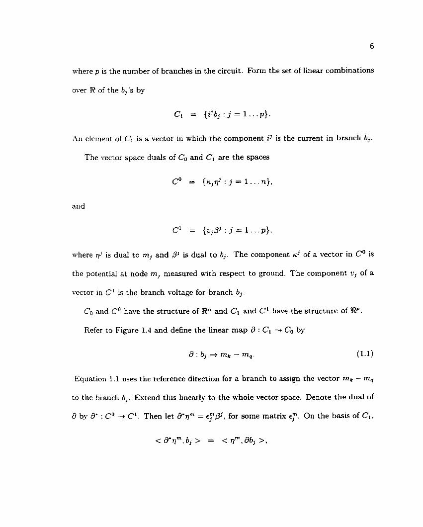
Refer to Figure 1.4 and define the linear map a : CI -+ Co by

Equation 1.1 uses the reference direction for a branch to assign the vector m k - m,

to the branch b j . Extend this linearly to the whole vector space. Denote the dual of

a by 8 : C0 + C1. Then let 6"qm = ~ y p j , for some matrix c?. On the basis of C1,

Figure 1.4: Boundary Map

= < q r n , r n k - m , >:

= q-c.

where rnc and m, are the bounding nodes of branch b,. The (m , j) entry in €7 is 1

if branch j is incident on node my -1 if branch j leaves node m and 0 if branch j

doesn't touch node m.

Let i E C1 : i = i 'b j . Then

for h = h'm[ E Co. So,

Also. let 11 E CO. A = ~ ~ q . Then? for some v = veae in C1,

So.

The above formalism now provides a way to express Kirchhoff's laws in algebraic

form. Consider Equations 1.3 and 1.4. he is the net current into node mc, so a vector

i E C, satisfies Kirchhoff's current law if i E kera. That is, if he = 0, t? = 1 . . . n. The

kernel of a can be computed from Equations 1.8, where the requirements on the i j ' s

are ijc: = 0.

Now consider Equations 1.1 1 , 1.12, and 1.13. The image of B can be computed

from these equations. Remember that the (j, k) entry of 4 is 1 if branch k is incident

on node j, -1 if branch k leaves node j and 0 otherwise. So VA: is the difference in

the bounding node potentials of branch k. Thus? Kirchhoff's voltage law can be

stated by requiring tt E imam. The requirements on the components of v are given

by Equation 1.13.

Kirchhoff's laws are expressed algebraically in terms of the operators a and 8,

which depend only on the topology of the graph. Hence the restrictions that the laws

place on the possible dynamics of the circuit are completely topological in origin.

Tellegen's Theorem is a classical theorem that states that the net power delivered

to the circuit by the circuit components is zero. Since the theorem only depends on

Kirchhoff's laws, it is a topological theorem.

The power for a circuit element is given by vji' (single component, so no sum on

j ) . where u j is the voltage across the j ' th component and ij is the current through it.

For a circuit, the total power is the sum of the power in each branch. Given a state

vector, ( i ,v) with i E Cl and v E Ci , the total power is ijvj (sum over j = I . . . p )

or, in terms of the canonical pairing, the total power is < v, i >.

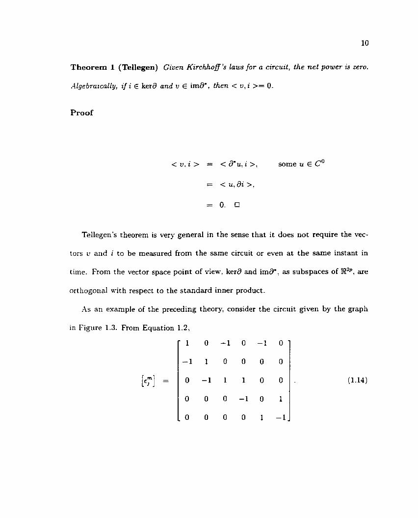
Theorem 1 (Tellegen) Given Kirchhoff's laws for a circuit, the net power is zero.

Algebraically, if i E kera and v E imam, then < u,i >= 0.

Proof

< v.i > = < aWu,i >, some u E C0

= < u , d i > ?

= 0. 0

Tellegen's theorem is very general in the sense that it does not require the vec-

tors 21 and i to be measured from the same circuit or even a t the same instant in

time. From the vector space point of view, kera and imam- as subspaces of 8 2 p . are

orthogonal with respect to the standard inner product.

.As a n example of the preceding theory. consider the circuit given by the graph

in Figure 1.3. From Equation f -2,

Equation 1.14 gives

where 11 = K ~ + E C? This gives

In turn, this gives the conditions

which is just Kirchhoff's voltage law in loop form. With two conditions on a 6

dimensionat vector space, dim(irna0) = 4.

kerd is given by

where i = i'b, E C1. This gives the conditions

This gives dim(kerl3) = 2.

1.2 Constitutive Equations

The circuit that we are concerned with contains resistors, capacitors. inductors and

operational amplifiers (op-amps). Table 1.1 shows the schematic for these circuit

elements.

Resist or

Capacitor

Inductor

Gyrator

Op-Amp

Table 1.1: Schematics of Basic Circuit Components

A resistor is a component that relates current to voltage

for some function f not necessarily invertible. Most commonlyy resistors in a circuit

are linear with

v = iR.

where R is the reszstance of the resistor. I t is a characteristic of the material the

resistor is made of.

Capacitors relate voltage to charge

Capacitors are also usually linear

where the constant, C, is the capacitance of the capacitor. It is a characteristic of

the dielectric separating capacitor plates.

Inductors relate magnetic flux to current

XIagnetic AIL. is not Lery conveniently measured, so differentiate 1.15 with respect

to time

d4 d f d i - = -- dt di dt '

.A changing magnetic flux produces a voltage: and we define L = g. Equation 1.16

can be written

L is usually a constant.

-4 gyrator is a two port element defined by

where G is the conductance (reciprocal of resistance). If port 2 is terminated by a

capacitor with capacitance C: equations 1.17 and 1.18 become

where q2 is the charge on the capacitor. Differentiate 1.20 with respect to time

Using 1.18 and solving for ul: Equation 1.22 is

Equation 1.23 is the constitutive equation for an inductor. Thus, when port 2 is

terminated by a capacitor, a gyrator behaves as an inductor with inductance 5. This

is important, since the quality of a gyrator simulated inductance can be considerably

higher that that of a traditional wirewrapped coil inductor. This means less power

dissipation and more accurate output. See Bruton [5] for a discussion on the quality

of a n inductor and simulated inductor. The circuit for a simulated inductor is shown

in Figure 3.5, and is used in the circuit described in Chapter 4.

.4n operational amplifier (op-amp) is defined by the relations

where A is some large constant on the order of 104 to lo6. It is assumed that

-E < L:, < E, where E is the power supply voltage. An equivalent circuit is given

by figure 1.5.

Figure 1.5: Equivalent Operational Amplifier Circuit

Circuit 1.5 facilitates the use of Kirchhoff's laws when an op-amp appears in a

circuit.

Since .A in equation 1.26 is large, it is often useful to assume A = oc and

1,' . - 2: - - = 0. Then the op-amp is described by

An assumption implicit in equations 1-27: 1.28, and 1.29 is that v, will be whatever

is necessary to maintain vi - v, = 0. These equations describe an ideal op-amp.

1.3 Power and Energy

The instantaneous power delivered to a circuit component is defined by

for a branch voltage v and branch current i. From a mechanical viewpoint, power is

the rate at which work is being done on a component by the rest of the circuit. This

is writ ten as

where C17 is the work. For a circuit with resistors: inductors and capacitors, the work

being done by the circuit on the components in changing the state from ( i ( to) , v(t0))

to ( i ( t ) , ~ ( t ) ) along a path r is

The first sum in Equation 1.30 gives the energy change in the inductors and the

second sum gives the enerm change in the capacitors. If the path I? is closed, then

the first two ter~ns of Equation 1.30 are zero and

So any energy absorbed by the inductors or capacitors is returned to the circuit. The

resistor branches, however, always absorb energy. This is seen by noting that the

integrand in Equation 1.31 is always positive. Hence the integral is always positive.

This means that the circuit always does positive work on the resistors. This is called

dzssipation. The energy absorbed by the resistors is converted to heat. This is a

non-reversible process. so the energy is not recoverable by the circuit.

The fact that inductors and capacitors return the energy they absorb leads us to

define the energy of a circuit by

By Tellegen's theorem. P = = 0 for the circuit as a whole. From Equa-

tions 1.30 and 1.32

So that

This shows that the energy dissipates in a circuit through the resistors.

19

1.4 The Brayton-Moser Equations for a Circuit

1.4.1 Resistor, Inductor, Capacitor Circuits

The purpose of this section is to derive a set of ordinary differential equations that

describe how the state of the circuit changes with time. These equations were first

derived by Brayton and Moser in [.I]. The following geometric formulation of the

theory was done by Smale in [14].

Denote the subspace of CI of currents in resistor branches by R , in inductor

branches by L. and in capacitor branches by C. Denote the subspace of C1 of

voltages across resistor branches by R', across inductor branches by C' and across

capacitor branches by C'. The voltage and current subspaces are dual for their

respective components and

CI x C1 = (R x C x C) x (a' x L' x C') .

Let I< = kerd x i m 3 . The resistor characteristic for each resistor branch is a one

dimensional submanifold of R x R' defined by

where p refers to the branch the resistor is in. The product A of the Ap's is a closed

submanifold of R x R'. Let r' : K + R x 'R' be the natural projection. Then

C = x 1 - l ( A ) is a submanifold of K. This is the space of physical states of the

circuit.

Let i.r : C i L x C' be the natural projection. For every point x E C such

that Dn(x ) : TzC + TrcZl (L x C') is an isomorphism, rr is a diffeomorphism for a

neighbourhood of x. For the purposes of Brayton-Moser theory, it is assumed that

T; is a global diffeomorphism. in other words, C is covered by a single coordinate

chart given by 7.

The previous statement relies on the truth of the following proposition.

Proposition 1

dim@) = dim(C x C*).

Proof

First? we show that dim(K) = p. where p is the number of branches.

and

ke r (8 ) has dimension 1, since the only way that all voltages can

be zero is when all node potentials are the same. dim(C1) = p and

dim(Co) = n, so Equations 1.34 and 1.35 give

Using the fact that dim(hY) = dim(ken3) + dim(ima0) and Equa-

tion 1.35. we get

Then

dim(C) = dim(K) - dim(R),

= dim(L x C'). CI

Define the metric J on C x C' by

where the sum over X is over the inductor branches and the sum over y is over the

capacitor branches. LA is the inductance in branch X and C, is the capacitance in

branch 7. Now define I = T ' J , the pullback of J to E by the natural projection. At

the points for which D7i is an isomorphism, I is nondegenerate.

Define the potential one form on C by

where the sum over p is over the resistor branches.

By Tellegen's theorem, x, u,diJ = 0 since it's a one form on K and so vanishes

on vectors tangent to C. Rewrite this as

Now.

Using Equation 1.39, Equation 1.38 can be rewritten as

Or. using the definition of dP in Equation 1.37, we get

Yow. v~ = L*% and i7 = 3 so that Equation 1.41 becomes

Or.

where Sp = ( 1 . The vector field X p is the tangent vector field to the trajec-

tories of motion of the circuit so that Equation 1.43 is the equation of motion for

the circuit. Written out explicitly, they are a set of ordinary differential equations

on the manifold C. These are the Brayton-Moser equations.

Classic Example

Consider the circuit in Figure 1.6 and its graph in Figure 1.7.

Figure 1.6: Damped Harmonic Oscillator Circuit

Figure 1.7: Graph for Damped Harmonic Oscillator Circuit

-4 state vector for this circuit is x = ( i ' , i 2 , i 3 , q , u2,v3) E S6. Kirchhoffk laws

are given by the matrix from Equation 1.2.

and

So i E kerd if

And v E imd' if

[a] = polT =

I -1 0

1 -I

So,

= span{& +&I +ai33, - &,.a,, - &,I.

The resistor characteristic is given by vz = i2 R, so that

A = {(i2 , P *2 R ) } .

And

Hence, the natural projection 7i : C -+ C x Cw is a diffeomorphism. Brayton-Moser

theory then applies.

On C ,

This gives the Brayton-Moser equations as

1.4.2 Resistorless Circuits

In the case where a circuit has no resistors, the power dissipated is zero. That is,

e n e r o in the circuit is conserved. In terms of mechanical systems the motion of the

system can be shown to be due to the influence of a potential that is analogous to

the electric field energy stored in the capacitors.

\Vith no resistors,

and

If T; : X i C x C' is a diffeomorphism, then the i7's are linear functions of the 2''s.

The equations of motion are then given by the vector field

Consider the vector space Q x C1 x C'. where Q is the vector space of the net

amount of charge to flow through the inductors. The components of Q are qX, which

is the net charge to flow through the X'th inductor so that Q* = i*. Let

Then.

n (C) = c,

where

- A - X q 7i : (q , I , z ? u A , u ~ ) * ( iA,i7,vA,uT).

The vector field for the circuit equations of motion is then given on by

Note that r.xp = Xp. The last two sums in Equation 1.18 give

These integrate to give

which are the constitutive equations for the capacitors in the circuit. Restricted to

the surface defined by Equation 1.49,

where we have made the substitution

remembering that i' and qT are linear functions of the iA:s and the qA's respectively.

Equation 1.50 is a vector field defined in terms of the inductor branches only.

Since q* = i*: the space Q x L is the same as the tangent bundle, TQ, of &.

Let F = xA LAqAd+. In terms of mechanical systems, this is the force field on &

that produces the motion given by the vector field xp. Then

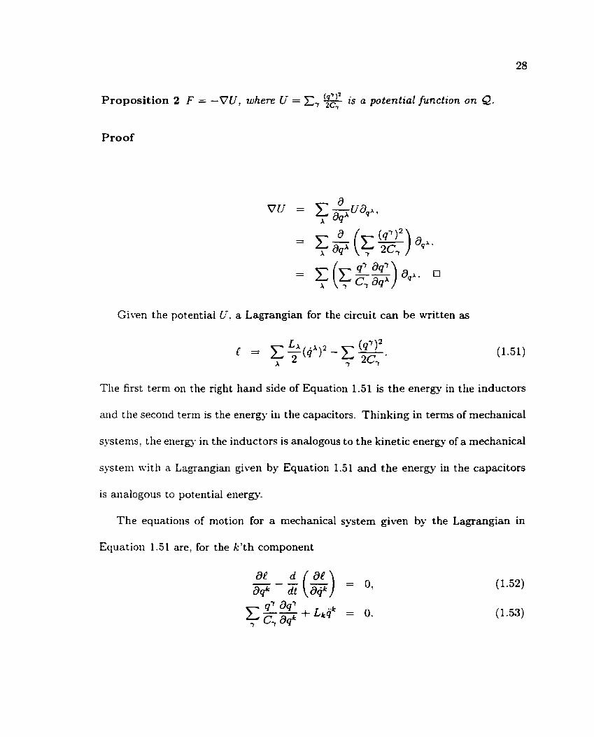
Proposition 2 F = -VU, where Li = x, is a potential function on Q.

Proof

Given the potential 0-: a Lagrangian for the circuit can be written as

The first term on the right hand side of Equation 1.51 is the energy in the inductors

and the second tern1 is the energ)- in the capacitors. Thinking in terms of mechanical

systems, the energy in the inductors is analogous to the kinetic energy of a mechanical

system with a Lagangian given by Equation 1.51 and the energy in the capacitors

is aiialogous to potential enerm.

The equations of motion for a mechanical system given by the Lagrangian in

Equation 1.51 aret for the k'th component

The Brayton-Moser equations for a resistorless circuit are given by the vector

field xp in Equation 1.50. Rewritten with qL = ik, the equations are

Or.

Equations 1.53 and 1.54 are identical. We say that the circuit is an electric circuit

analogue of the mechanical system given by the Lagrangian in Equation 1.51.

1.4.3 Op-Amps in a Circuit

To facilitate the application of Brayton-Moser theory for circuits containing op-

amps it is useful to introduce two more types of circuit elements: the nullator and

norator. These are defined in Bruton [5].

Figure 1.8: The Nullator

The schematic for a nullator is shown in Figure 1.8. The constitutive equations

are

The norator is shown in Figure 1.9.

Figure 1.9: The Norator

The constitutive equations are

= arbitrary,

2' = arbitrary.

Considering the equations for an ideal op-amp given in 1.27, 1.28, and 1.29, we

can use a nullator and a norator to represent an ideal op-amp. See Figure 1.10. This

device is called a nullor.

The nullator represents the inputs of an ideal op-amp, since there is no current

into them and no voltage drop across them. The norator represents the output, since

Figure 1.10: The Nullor Op-Amp

there is no current constraint, and the output of the ideal op-amp will be whatever

is necessary to force a zero voltage drop across the inputs.

For the purposes of writing the Brayton-h'loser equations, the nullator and nora-

tor can be included as resistive elements. The nullator has a resistor characteristic

of (0: 0) and the norator has characteristic (i, v). An o p a m p is therefore made up

of two resistive elements that toget her produce a two dimensional characteristic (the

whole i - c* plane given by the norator). So the set of physical states, C, can be con-

structed in the same manner with its dimension still being equal to the dimension

of L x C'.

Chapter 2

The Circuit Analogy

I t was sho~vn in section 1 A.2 that a circuit with no resistors is the electric analogue

of some mechanical system with Lagrangian 1.51. It is obvious that this is a Hamil-

tonian system with momenta given by the Legendre transformation p , ~ = L*qA. The

converse problem is whether a Hamiltonian system has an electric circuit analog. The

rest of this thesis is devoted to studying the electric circuit analogue of a particle in

with potential LT = ( X + ~ - Z + Q ) ' ,, - and the nonholonomic constraint i = yx.

2.1 Unconstrained System

The basic dynamical system for which an analogy will be discussed is a particle in

under the influence of the potential Cr = (2+y+z+ ,, '". where Q and C are constants.

-4s shown in Section 2.4.2, this is the potential given analogously by the energ?. in a

capacitor.

The circuit shown in Figure 2.1 is a capacitor in parallel with three inductors (of

equal inductance). From left. to right the branches will be referred to as as the w:

x. y, and 2 branches. The electric field energy of the capacitor is $: where w is the

charge on the capacitor and C is its capacitance. The magnetic field energy of each

L ( i * ) = inductor is 7, where xi is the current through the i'th inductor.

Figure 2.1: Harmonic Oscillator Circuit

Kirchhoff's Current Law at node 1 gives the equation

cr- j - y - f =0.

Or. after integrating,

U : - Z - y - Z - Q = ( ) , (2.1)

where Q is a constant of integration. The electric field energy of the capacitor is

then

Using Brayton-Moser theory, or applying Kirchhoff's voltage law: the equations

for the circuit are

Now consider the mechanical system consisting of a particle of mass m in

under the infhence of a force due to the potential

where Q and C are constants. The Lagrangian for the system is

and the Euler-Lagrange equations are

Since these are identical to the circuit equations, the circuit is an electric analogue

of the mechanical system.

Let

Then

i L z + g + : -

Then equations 2.2, 2.3. and 2.4 can be added to give

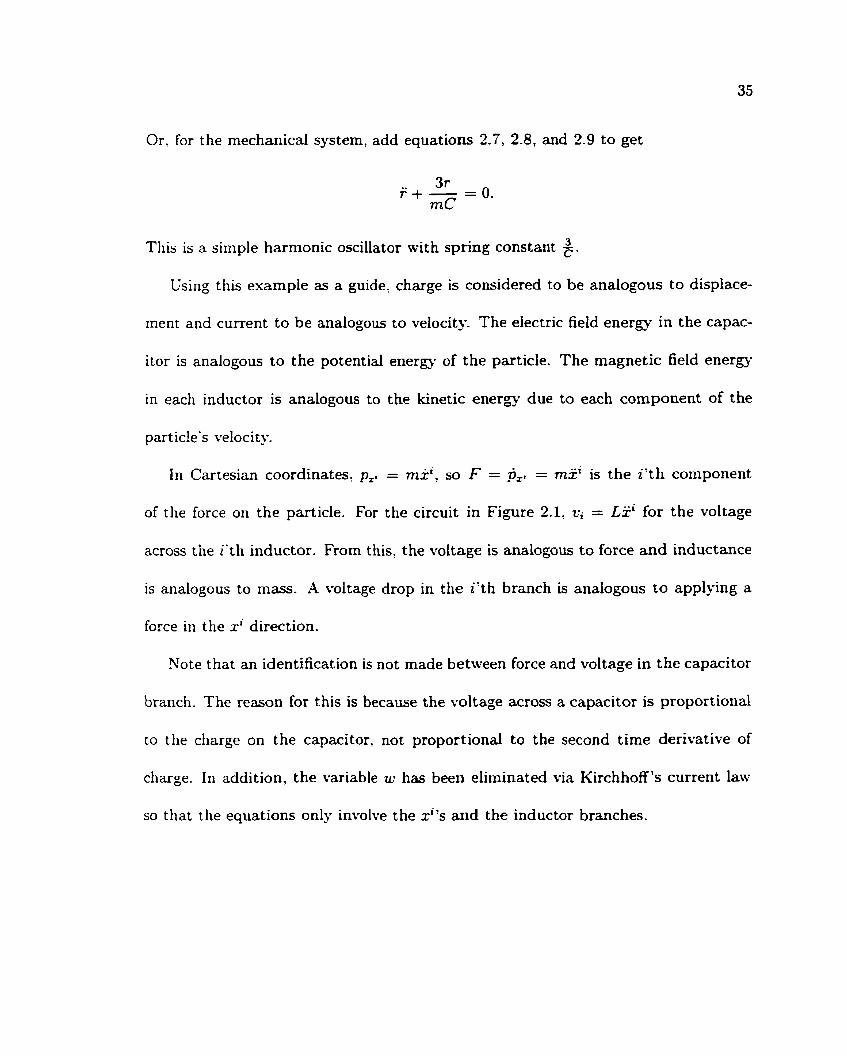
Or, for the mechanical system, add equations 2.7, 2.8, and 2.9 to get

This is a simple harmonic oscillator with spring constant 6. Using this example as a guide: charge is considered to be analogous to displace-

ment and current to be analogous to velocity. The electric field energy in the capac-

itor is analogous to the potential energy of the particie. The magnetic field energy

in each inductor is analogous to the kinetic energy due to each component of the

particle's velocity.

In Cartesian coordinates, p,. = mi', so F = ?=. = mx' is the i ' th component

of the force on the particle. For the circuit in Figure 2.1: ui = Lx' for the voltage

across the i'th inductor. From this, the voltage is analogous to force and inductance

is analogous to mass. A voltage drop in the i'th branch is analogous to applying a

force in the xi direction.

Note that an identification is not made between force and voltage in the capacitor

branch. The reason for this is because the voltage across a capacitor is proportional

to the charge on the capacitor, not proportional to the second time derivative of

charge. In addition, the variable w has been eliminated via Kirchhoff's current law

so that the equations only involve the xi's and the inductor branches.

2.2 Constrained System

-4 constraint is given by specifying a one form, 4, on configuration space and requiring

that all velocity vectors lie in the kernel of the one form. If q is an exact one form,

then the constraint determines a surface in configuration space that the particle must

remain within. This is called a holonomic constraint. -4 nonintegrable constraint is

called nonholonomic.

The constraint imparts a force on the particle to cause its motion to always satisfy

the constraint. According to D' Alembert7s principle. this constraint force is always

perpendicular to the motion of the particle, and hence does no work on the particle.

The vector field, X = g : ~ , where g is the standard metric on PR3? is perpendicular to

all motions of the system. The force of constraint is given by the field F = AX, where

X is an undetermined scalar function on configuration space. D'Alernbert's principle

determines the direction of F, but it's magnitude can v q from point to point,

hence the function X is necessary, X is sometimes called a Lagrange undetermined

multiplier.

In order to build an electric circuit analog of a mechanical system with a con-

straint given by d, the constraint force, F, must be explicitly included in the circuit.

Since a force is analogous to a voltage drop, each inductor branch in the circuit

must have a voltage drop of the same magnitude as the corresponding component of

the constraint force. The following is based on the unconstrained system described

above.

Consider the nonholonomic mechanical constraint

# = d z - ydx,

which can also be written as

D' Alembert 's principle gives the force that maintains this constraint as

F = A(-y, O,1),

where X is a Lagrange undetermined multiplier.

Figure 2.2: Constrained Harmonic Oscillator Circuit

To build a circuit that emulates constraint 2.11, a voltage drop of magnitude

-yX needs to be added to the x branch and another voltage drop of magnitude

X ill the z branch. A circuit that symbolically satisfies the constraint is shown in

Figure 2.2. In the z branch a voltage controlled current source has been inserted

to force the constraint t o be satisfied. Since v= = Li , the voltage across the r

inductor is determined by the changing current produced by t h e current source. In

order for Kirchhoff's voltage law to be satisfied there must be a voltage drop across

the current source. Let this voltage drop have magnitude A. Now add a voltage

controlled voltage source to the x branch to give a voltage d rop of -PA. Since the

constraint force does not have a y component, no additional voltage drop in the y

branch is necessav.

The Lagrangian for the constrained mechanical system (Equation 2.11) is the

same as the Lagrangian for the unconstrained system (Equation 2.6). Taking the

nonholonomic constraint into account, the equations of motion are modified by the

constraint force. Thus, the equations are

Using Kirchhoff's voltage law, the equations for the circuit in Figure 2.2 are

Identifying m with L: equations 2.12, 2.13, and 2.14 are identical to equa-

tions 2.15. 2.16, and 2.17.

Eliminating X and using E = y x + yx (which comes from differentiating equa-

tion 2.1 l ) the final form of the Euler-Lagrange Equations 2.12, 2.13 and 2.14 are

Hamilton's equations for the circuit can be written by letting p,. = Lx' and

pIL' = u. c- Kirchhoff's voltage law then gives

The constraint f - y x = 0. written as a constraint on phase space, is p= - yp, = 0 .

Using Kirchhoff's Current Law, eliminating A: and using 6, = jrp,+y@, the equations

can be written in Hamiltonian form as

x + y t : + Q p, = - C

We now derive Hamilton's equations for the mechanical system using the method

of Bates and ~ n i a t ~ c k i [2] . The

h =

Hamiltonian is

with constraints

w - x - y - r - Q = 0,

dt - ydx = 0.

The first constraint is holonomic, so it can be substituted directly into the Hamil-

tonian to obtain

To eliminate the nonholonomic constraint we restrict our attention to the sub-

manifold of phase space that satisfies the constraint. Namely the set

df = {(x, y, r , p., p,, p;) : p; - yp, = 0).

Since Jf is the graph of a function, x, y! I, p,, and, p, are coordinates.

We also only consider motions of the system that satisfy the constraint form

pulled back to phase space by the cotangent bundle projection. Thus, the allowable

motions must have tangent vectors in the distribution

H = ker{ra(d= - y d x ) } n T M

= ker{dr - ydx) n T M ,

= span{y& +a,,a,,a,,,apJ.

where ;; is the canonical projection from T'Q + Q and & is the configuration space.

The canonical symplectic two form on phase space, T ' V , is

w = dx Adp, + d y A dp, + dz A dp,.

Hamilton's equations are

XJUJ = d h + Xl;'(dz - ydx),

where X is a Lagrange undetermined multiplier. Restricted to M . the canonical

symplectic two form is

Uar = d~ A dp, + d y A dp, - p,dy A dz + ydz A dp,.

Since u a t f I H = ;JH is nondegenerate, Hamilton's equations can be written as

where d h H is dh restricted to vectors in H. There is no term involving the Lagrange

multiplier since rrm(dz - ydx) (v ) = 0 for all v E H.

The Hamiltonian vector field, X, contracted with w,\1 is

X J U , = - p , d ~ + ( f p , - p,)dy - (yp , + y&)ds + ( X + y f )dp , + ~ d p , .

The differential of the Hamiltonian is

Evaluating the left and right hand sides of Hamilton's equations on H gives

y p : + x + y t z + Q ( d h . a,) = - C 1

m

Equating the appropriate left and right hand sides gives

These are four equations in five variables. To get the fifth equation, use the fact

that S E H so that

X = a(y& +a,) + b 4 +cap* + d h .

Equating coefficients with the Hamiltonian vector field for h

-u = xa, + @ay + 2; +p,a,, +pyap,,

gives

This gives us five linear equations in the five variables x, y, 2 , p,, p, which results

in Hamilton's equations

Identifying m with L shows that the circuit and mechanical system equations are

the same.

Chapter 3

The Circuit

3.1 The Components

The schematic for a circuit that obeys constraint 2.11 is shown in Figure 3.1. -4

larger diagram is shown in Appendix A.

Figure 3.1: Schematic for Constrained Harmonic Oscillator Circuit

The constraint to be realized is i - yx = 0. In other words, the current in the

z branch needs to be the product of the current in the x branch and the net charge

that has gone through the y branch. These quantities are first converted to voltages

for easier manipulation, then multiplied by a commercial multiplier. The output of

the multiplier is sent to a ~~ol tage controlled current source in the r branch.

Figure 3.2: Current to Voltage Converter

The circuit for converting current to voltage is shown in Figure 3.2. The output

is 21 = -iR. In the circuit shown in Figure 3.1: the non-inverting input is not

connected to ground. but to the output of a voltage multiplier. The purpose of this

will be made clear in the next section.

Figure 3.3: Integrator

Figure 3.3 shows the circuit used to convert charge to voltage. Current is the

time derivative of the net charge that has gone through a branch. Hence, charge

is given by the integral of current. The voltage across the capacitor is v ( t ) = 9, where q ( t ) is the charge on the capacitor with its time dependence explicitly shown.

The output of the operational amplifier is v = -$ Ji i ( t ' )dtJ . This circuit is called

an integrator.

Figure 3.4: Voltage Controlled Current Source

The voltage controlled current source is shown in Figure 3.4. This circuit draws

the current i = through a grounded load (represented by the resistor labelled

'L04D1). For our purposes, the grounded load is the entire circuit.

Figure 3.5: Simulated Inductor

The inductors in circuit 3.1 are simulated by the circuit shown in Figure 3.5. The

inductance is given by L = R2C. See Bruton [5] for a detailed explanation of this

circuit.

3.2 The Constraint in the Circuit

IVe start with the standard harmonic oscillator circuit as described in Chapter 2 and

shown in Figure 2.1. The current in the x branch is converted to a voltage using the

circuit in Figure 3.2. The output will be denoted by

The current through the y branch is integrated to give

where y = $ Ji i(tt)dt '- the net charge through this branch. The outputs, u, and v,:

go to the inputs of another voitage multiplier.

The output of the multiplier is scaled by &. This serves the double purpose of

keeping the voltage to reasonable values and fixing the units. Since the output of

the multiplier is the product of two voltages, the scaling factor needs units of

in order for the output to have units of volts. At this point we have

This goes to the input of the voltage controlled voltage source, where the current

through the 2 inductor is forced to be

Or, writing i, = x and i: = 5

Kirchhoff's voltage law around a loop including the r branch shows that there is

a voltage drop X across the current source. The constraint, as given by Equation 3.17

gives an analogous constraint force of

Equation 3.2 shows that

output of the integrator

a voltage drop of -A- is needed in the x branch. The

is -:. This and the voltage across the current source, A:

are used as inputs to another multiplier. The output of the multiplier is then

The voltage in 3.3 is precisely what is needed. The output of the multiplier is then

sent to the noninverting input of the current to voltage converter in the x branch to

provide the necessaq voltage drop.

The initial conditions that can be set for the circuit are

where D is a parameter that we can control (the charge on the capacitor). IVith

these initial conditions, Q = 0 in equation 2.1.

To achieve condition 3.4, a voltage, v. is placed across capacitor Cz (Figure 3.1)

to induce the charge trCz on the capacitor. This charge corresponds to an initial y

displacement in the analogous mechanical system. There is an initial force acting on

the particle due to the potential given in Equation 2.5. This force is

This implies that the voltage applied across C2 also needs to be applied across C1 so

that each inductor will have a voltage of magnitude 9 applied across it. Note that

C2 = C1 SO that the initial conditions in terms of the charges on the capacitors are

equal.

The initial conditions are valid for t < 0. At t = O1 the switch is flipped, and the

capacitors are brought into the main circuit.

3.3 Building the Circuit

This section is devoted to the little details necessary to make the circuit function.

The circuit was built on a protoboard in an aluminum case for shielding. The

simulated inductors were wire mapped on separate perf boards for modularity.

The op-amps used in the circuit and inductors are LF347 quad op-amps. In-

dividual op-amps could be used: but we found that the quads reduced the signal

propagat ion time enough to eliminate the self oscillations experienced with the sin-

gle op-amps. -41~0, the quad op-amps allowed for a more compact and tidy circuit.

In order to filter out power supply noise, O.1pF capacitors were placed across

the op-amps's positive power supply input and ground. The same was done for the

negative power supply input.

100pF polarized capacitors were placed from the positive power supply line to

ground. Same for the negative power supply line.

-4 0.01pF capacitor was placed in parallel with the negative feedback resistor on

the current source to reduce self oscillations in that circuit.

The capacitors used for the circuit were measured to be within 1% of each other.

The capacitors used for the inductors had values with a maximum difference of 5%

of each other. The resistors for the c i rc~i t had a maximum difference in value of

0.04%. For the inductors, the difference was 1%.

The switch used is a 4 pole, singie throw mechanical switch. No noise was evident

when switching. A digital switch should be used for a sensitive experiment.

3.4 The Experiment

The purpose of building this circuit was to test to see if an electric circuit analogue of

a mechanical system is accurate enough to claim that the dynamics of the circuit are

the same as the dynamics of the mechanical system. Even though the equations for

the circuit and the mechanical system are identical, the circuit experiences energy

loss due to the inherent resistance of conductors. So we cannot expect the actual

dynamics to be identical.

The experiment was run for various initial values of y and with alI other initial

conditions zero. This restriction was for the purpose of simplicity. Data was col-

lected for x and y using a computer oscilloscope. t was computed using the circuit

constraint from Equation 3.1, rather than measured directly from the circuit. This

was also done for simplicity. The error in computing the value rather than measuring

i t directly is the accuracy that one can measure the resistance for the resistors in the

current source. This is 0.005% for 1KQ resistors.

The data for x, y, and 2 were computed numerically from the data gathered

from the circuit. The programs for computing x and y are listed in Appendix B. The

program for computing z is identical to the one for computing x: except for filenames.

Following are the figures representing the data. Each experimental result is plotted

with the theoretical result, as computed numerically by Maple using Equations 2.18,

2.19, 2.20, and the circuit constraint given in Equation 3.1. See Appendix B for

the Maple code. Also included in the figures are the results of computing the total

energy of the circuit as a function of time, plotted with the theoretical value of the

energy computed from the Maple data.

It is apparent from the figures that the experimental da ta matches up reasonably

well with the theoretical results. A small phase difference is noticeable, likely due to

extra capacitance from the proto-board and errors in the simulated inductor values.

The computer oscilloscope sampled data fast enough to often record the same

value for several consecutive time steps. This caused the numerically computed

graphs for x (Figure 3.6)$ z (Figure 3.8): and y (Figure 3.10) to appear itjagged".

I11 any Hamiltonian system, the energy remains constant. As can be seen in the

energy graph (Figure 3-12)? however, the computed curve is definitely not constant,

leaving some doubt as to the accuracy of the numerical method used by Maple.

The measured energy is even worse. The problem likely lies in the accuracy of the

the current to voltage converter, the charge to voltage converter, and the voltage

controlled current source.

Figure 3.6: x Displacement

Figure 3.7: y Displacement

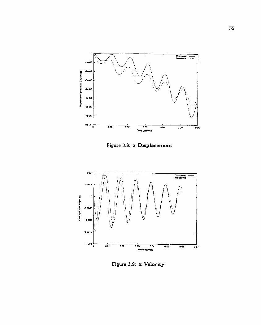
Figure 3.8: z Displacement

Figure 3.9: x Velocity

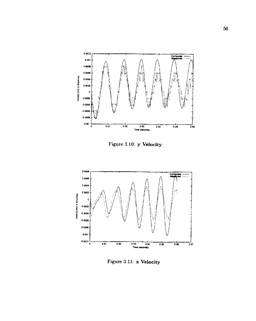
Figure 3.10: y Velocity

Figure 3.1 1: z Velocity

Figure 3.12: Energy of the Circuit

Chapter 4

Conclusion and Further Work

The goal of this project was to decide whether it was possible to build an electric

circuit analogue of a Hamiltonian system with a nonholonomic constraint and to

determine whether such a circuit would be useful in providing information about

the dynamics of the system. It is clear from the above results that such a circuit

can be built with output accurate enough for running experiments. Higher quality

output can be obtained by having the circuit built on a printed circuit board with

components of tighter tolerances. This should give a better energy graph as well.

-4s a part of this process. a theory for writing the differential equations describing

a circuit ' s dynamics was reviewed. Resistorless circuits are shown to be analogous

to Harniltonian systems. The converse problem of deciding whet her a Hamiltonian

system has an electric circuit analogue is done on a case by case basis, though it

should be possible to characterize certain Hamiltonian systems as having electric

analogues. Further to this is determining what types of constraints can be realized

in an electric circuit analogue. The ultimate goal would be to determine whether or

not it is possible to construct an electric analogue of a Hamiltonian system with a

nonlinear, nonholonornic constraint.

To further test the implementation of an electric analogue as many invariants as

possible should be computed for the mechanical system and measured from the cir-

cuit. Invariants for holonomic systems come directly from symmetries in the system

(Yoether's Theorem). For nonholonomic systems, Noether's Theorem applies when

the invariant function has its Hamiltonian vector field in the distribution anhilated

by the constraint. Otherwise, the best that can be hoped for is a reduced constraint

distribution, A, that is integrable. See Bates and ~ n i a t ~ c k i [2] .

In the case studied here, the symmetry is in the direction 3: - 3, so that the

reduced constraint distribution is given by

where (s. y. p,: p,) parameterize the reduced phase space, 1u. H drops a dimension

in the hyperplane y = -1 so that a direct application of the theory in Bates and

~ n i a t y k i (21 is not straightforward. Further analysis could be done using the method

in Bates [3].

On the topic of symmetr). reduction, an interesting side note is found by examin-

ing the Harniltonian system corresponding to the unconstrained harmonic oscillator

circuit in Figure 2.1. The Harniltonian is

where L and C are constants. This system admits translational symmetries in the

directions a, - & and a= - a,. The reduced Hamilton's equations are

ace. These are the sam where q and pq parameterize the reduced phase sp .e equations

we get by replacing the three parallel inductors in the harmonic oscillator circuit by

a single equivalent inductor. In a sense! the process of replacing parallel inductors

with a single equivalent inductor "reduces?' the circuit. It would be interesting to see

what the reduced circuit would be for the system studied in this thesis, if one exists.

Bibliography

[I] V. -4rnold. Mathematical Methods of Classical Mechanics. Springer-Verlag,

New York. 1989.

[2] L. Bates and J. ~ n i a t ~ c k i . Nonholonomic reduction. Reports on Mathematical

Physcis, 32:99-115, 1993.

[3] L. .\I. Bates. Examples of singular nonholonomic reduction. Reports on Math-

ematical Physics, 42:231-247, 1998.

[4] R. Brayton and J. Moser. A theory of nonlinear networks. I 11. Quart- Appl-

Math. 22:l-33, 81-104. 1964.

[j] L. T. Bruton. RC- Active Circuits. Theory and Design. Prentice-Hall, Engle-

wood Cliffs, Pi. J., 1980.

[(i] R. H. Cushman and L. M. Bates. Global Aspects of Classical Integrable Systems.

Birkhouser Verlag, Basel, 1997-

[7] L. Chua. C. Desoer, and E. Kuh. Linear and Nonlinear Circuits. kLcGraw-Hill,

Kew York, 1987.

[8] A. P. French. Vibrations and Waves. W. W. Norton and Company: Inc., New

York, 1966.

[9] H. G. E. Graumann. Rat tleback symmetry reduction. blaster's thesis, Univer-

sity of Calgary, Dept. of Math, 1994.

[lo] J. Marion and S. Thornton. Classical Dynamics of Particles and Systems. Saun-

ders College Publishing, Orlando, 1995.

[ 1 11 J. Sf arsden and T. Ratiu. Introdvction to Mechanics and Symmetry. Springer-

Verlag, New York, 1994.

1121 L. Pars. A Treatise on Analytical Dynamics. Ox Bow Press, Woodbridge, CT,

1979.

[13] R. Rosenberg. Analytical Dynamics. Plenum Press, New York, 1977.

[Id] S. Smale. On the mathematical foundations of electrical circuit theory. J-

Dzfferential Geometry, 7: 193-210, 1972.

Appendix A

Parts List

Part LF 347 Quad Op-Amp AD633 Multiplier IKR Resistor 100pF Capacitor 1pF Capacitor 0. lpF Capacitor 0.01pF Capacitor Potentiometer 4 Pole Switch 12V Power Supply 9V Battery

Quantity 1

Table A.1: Parts for Circuit

Quantity LF 347 Quad OpAmp 3.3KS1 Resistor 0.68pF Capacitor 0.1pF Capacitor

Table A.2: Parts for Each Simulated Inductor

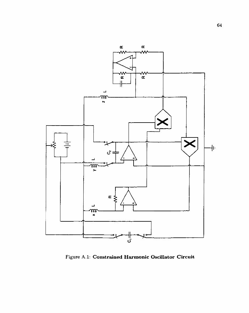
Figure -4.1: Const rained Harmonic Oscillator Circuit

Appendix B

Computer Programs

c FORTRAN Program to compute x from xdot data

c using Simpson's rule

real xdotl,xdot2,xdot3,deltat

real xl,x2,~3,tl,t2,t3

integer i

c time s tep given by the data file

deltat=0.000250

c Simpson's rule

c Essentially doing the integration two times, but

c vith different starting points.

do i=4,240,2

xdotl=xdot2

xdot2=xdot3

t l=t2

t2=t3

read(lO,*) t3,xdot3

x2=x2+deltat*(xdotl+4.*xdot2+xdot3~/3.

vrite(11,lOO) t3,x2

read(lO,*) t3,xdot3

~3=~3+deltat*(xdotl+4.*xdot2+xdot3)/3.

write(l1,lOO) t 3 ~ 3

end do

close (10)

close (11)

end

c FORTRAN program to compute ydot from y data

c using numerical differentiation

real yLy2,y3,y4,y5,h,ydotSt

integer i

c time step given by the data

deltat=0.000250

write(11.100) t-2.*deltat,ydot

y1=y2

y2=y3

y3=y4

y4=y5

end do

close (10)

close (11)

end

#Maple Code for Numerically Solving the Euler-Lagrange

# Equations

#

#Set some constants

R1:=1E3;R2:=1.0044E3;L:=7.45;C:=0.99E-6;h:~0.000250;

#

#Define the system as a set of first order ODE'S

sys:=(diff (x(t) ,t)=v(t),

diff (y(t) ,t)=w(t),

diff ( v ( t ) ,t)+l0*~2*Cx(t)+y(t)+z(t))*~R2*1O*C+R1*y~t~)

/(~*((R2*10*C)-2+(Rl*y(t))-2))+

Rla2*y(t) *v(t) *v(t) /( (R2*lO*C) -2+(~l*y(t) ) -2)=0,

diff (v(t) ,t)+(x(t)+y(t)+z(t))/(L*C)=O,

diff (z ( t ) ,t)-~l*v(t)*y(t)/(R2*10*~)=0>;

#

#Set i n i t i a l conditions

inits:=~x(0)=0,y(0)=3.7*C,z(0)=0,v(0)=0,~(0)=0~;

#

vars:=Cx(t) ,y ( t ) ,z(t) ,v(t) ,v(t)3;

*

S:=dsolve(sys union inits~vars,type=numeric,output=listprocedure);

fx:=subs(S,x(t)) :fy:=subs(S,y(t)) :fz:=subs(S,z(t)) :fv:=subs(S,v(t)) :

fu:=subs(S,w(t)) :

#

A:=array(l. -240,l. -7) :

for i to 240 do

a:=fy((i-l)*h) :

b:=fv((i-l)*h) :

A[i, 11 :=(i-l)*h:

A[i,2] :=fx((i-l)*h) :

A[i,3] :=a:

ACi.41 :=fz((i-l)*h) :

A[i,5] :=b:

A[i ,61 :=fv((i-1)*h) :

A [i ,71 : =Rl*a*b/ (R2*1O*C) :

od:

#Write to a data file

fd:=fopen(linearnumdat,WRITE,TEXT):

writedata(fd,A,float) :

fclose(1inearnumdat):