An Effective Topological Adjustment on Vector Maps for AVL

BAO Yuanlu, LIU Zhenan, QU Jin Department of Automation, USTC, Hefei, 230026, China.

ABSTRACT Advanced Vehicle Location (AVL) needs accurate vector maps. This paper presents a discrete topological transformation to get vector map nonlinear geo-adjustment. The new algorithm adjusts a sample point by a sample point. At the time of adjusting one point, the algorithm also automatically adjusts all its neighboring area points within a block/polygon area keeping their topology. If the selected sample point set has enough distribution, then the vector map will have an accurate adjustment for all map points because the total nodes on the map is very limited on the vector map. Example shows the effectiveness of the new method on vector map automatic geo-adjustment.

Keywords: nonlinear adjusting, vector map, network topology, GIS, GPS

1. INTRODUCTION Digital times need digital maps and modern cities need intelligent transportation1-2. Lack of vector maps and accuracy of vector maps have become the bottleneck of developing digital city transportation and intelligent decision3. The important tasks of constructing digital city information systems are to speed the process of converting raster (or paper) into vector maps and to provide accurate vector maps for Advanced Vehicle Location (AVL).

To provide accurate vector maps for AVL, current vector map geo-adjusting algorithms take a global affine transform5-6. These algorithms may correct only linear errors of vector maps, but not nonlinear errors due to various reasons. It is noticed that the previously methods such as Least Mean Square (LMS) method5 and other optimal method6 intend to reduce or minimize the error summation of selective points by the limit of global affine transformation. Thus it can not exactly adjust a group of selective points to their corresponding accurate positions, see Fig.2. They only reduce the sum of their position errors, but never reach zero because of the nonlinear errors existed always on a vector map extracted from a raster or printed map.

In order to accurately correct both linear and nonlinear errors, this paper presents a novel approach of discrete topological geo-adjusting method to automatically complete accurate vector map geo-adjusting. The key of this method is to exactly adjust a group of selective points to their corresponding accurate positions on the vector map, and simultaneously to accurately and topologically adjust their neighboring areas.

2. AUTOMATIC MAP GLOBAL AFFINE GEO-ADJUSTING Map geo-adjusting is for improving vector map accuracy. The method is to use the recorded road locus by GPS to automatically adjust the vector traffic map. Select a group of n known points set G on map with their accurate position set Ĝ:

)},(,),,(),,({},,,{ 22211121 nnnn yxgyxgyxggggG LL == (1)

)}ˆ,ˆ(ˆ,),ˆ,ˆ(ˆ),ˆ,ˆ(ˆ{}ˆ,,ˆ,ˆ{ˆ22211121 nnnn yxgyxgyxggggG LL == (2)

Definition 1. An automatic vector map global affine geo-adjustment should adjust a selected group of points G to G*, for G closes to their known exact positions Ĝ as nearly as possible and simultaneously keeping the map topology.

Now, the goal is to find a liner topological mapping M(·) to map G onto G* as **

1*1

*121 },,,{)}(,),(),({)(:)( GggggMgMgMGMM n ===⋅ LL (3)

to minimizing optimal performance index ])ˆ())ˆ[(ˆ 21

*2**i

n

i iii yyxxGGJ −+−=−= ∑ = (4)

International Conference on Space Information Technology, edited by Cheng Wang, Shan Zhong,Xiulin Hu, Proc. of SPIE Vol. 5985, 598521, (2005) · 0277-786X/05/$15 · doi: 10.1117/12.657414

Proc. of SPIE Vol. 5985 598521-1

The mapping M(·) can be a global affine transform to map all nods (x,y) into (x*,y*) as follows:

⎩⎨⎧

++=++=

222

111

**

cybxaycybxax with 0

22

11 ≠baba (5)

Using an optimal approximation method such as improved Newton method or DFP method to find an optimal parameter [a1, a2, b1, b2, c1, c2] getting minimum J in Eq. (4). An effective algorithm in [6] takes mapping M(·) be a composition mapping, include only two kinds of mappings: a mapping ML(·) for expansion/contraction and movement, and a conformal mapping MR(·) for rotation, M(·) = MR(ML(·)) Note that M(·) always keeps vector map topology, an example for digital map linear geo-adjusting of city Chengdu city is show in Fig. 1 and Fig. 2.

The global affine transform belongs to a linear adjustment on vector maps. They cannot achieve the above objective (4) to zero. They reach optimal approximation in sense of the LMS with their algorithm limitations. When the source map error is minor, these algorithms may return good results, but they are still not ideal. When the source map error is large, these algorithms may not be satisfied or may fail.

Fig. 1. Using road locus to adjust a digital map Fig. 2. Adjusted digital map after Geo-adjusting

3. NEW DISCRETE TOPOLOGICAL ADJUSTING ON THE VECTOR MAP

The vector map accuracy depends only on the finite node point’s accuracy. The vector map must keep those nodes topology7. Thus, we propose a new discrete topological adjusting method for automatic vector map nonlinear geo-adjustment as follows.

Definition 2. A discrete topological geo-adjustment on vector map should adjust a selected group of points to their known exact geo-data (longitudes and latitudes) and simultaneously correct all nodes within its neighboring areas keeping the map topology.

Now the goal is to find a nonlinear topological mapping T(·) to map exactly G in Eq. (1) onto Ĝ in Eq. (2), i.e.

GggggTgTgTGTT nnˆ}ˆ,,ˆ,ˆ{)}(,),(),({)(:)( 2121 ===⋅ LL (5)

and simultaneously to adjust their neighboring areas keeping the map topology.

3.1. Dynamic neighboring block (polygon) Ak, k=1,2,…,n Assume the selected sample point set G has n points. Then, the algorithm has n steps, consequently, the transformation T(·) is decomposed as

)))((()( 121 LLL ⋅=⋅ − TTTTTT knn (6)

Proc. of SPIE Vol. 5985 598521-2

When, at the k-th step, before mapping Tk, the algorithm procedure Tk-1Tk-2…T2T1 has accurately adjusted k-1 sample points,

}ˆ,ˆ,ˆ{},,{ 121121 −− ⇒ kk gggggg LL (7) which have been and should be fixed during the following adjustment steps. On the k-th step mapping Tk(·) will adjust the point gk to ĝk and all nodes set, denoted as Sk = {si}, with node si on the block (polygon) Ak, i.e.,

kk gg ˆ→ , )(ˆkkkk STSS =⇒ when kk AS ⊂ and kk SS ⇒ when kk AS ⊄ (82)

In this section we solve first the question how to design block Ak. Obviously the sample points and their distribution is the key factor to determine the boundary of dynamic neighboring region Ak. They are set by the following rules.

The first block A1 is the whole map. The second block A2 is the whole map except the point ĝ1. The k-th block Ak (k≥3) is determined by the following rules shown in Fig. 3 and Fig. 4 where ĝi, i=1,2,…,k-1, have been adjusted for their respective gi, i=1,2,…,k-1. At k step let the line ĝiġk be the bisector of the angle ∠gkĝiĝk.. Then make a perpendicular line Lkĝi to the line gkġk pass point ĝi. The line Lkĝi divides the map into two half planes. Denote the half plane with point gk and iĝk. as Hk(ĝi). The block Ak is within Hk(ĝi), i.e.

)ˆ( ikk gHA ⊂ , 1,...,2,1 −= ki and I1

1)ˆ(−

== k

i ikk gHA , nk ,...,4,3= (9)

The discrete block Ak may be a limited region as a m-polygon, e.g., as shown in Fig. 4, where k=6, Ak = A6, is a quadrilateral ABCD with m = 4. Its m-boundary lines are Lkĝi, i∈{1,2,…,k-1}. There is always m ≤ k-1, For large m, we may have m << k-1. Of course it may not be a bounded region as shown in Fig. 5.

Fig. 3. Block region Ak on the half plane Hk(ĝi) (i<k) Fig. 4. Construction of block Ak (k=6)

3.2. Discrete Topological Adjusting procedure Tk, k=1,2,…,n The first two steps are trivial. The new algorithm essentially begins from step 3, as above Step k (k=3,4,…,n):

Step 1: Move the block A1 (the whole map) to complete the mapping T1 insuring )ˆ,ˆ(ˆ),( 111111 yxgyxg → is

)ˆ,ˆ(ˆ),(ˆ)(),(: 111111 yyyxxxsyxssTyxsT −+−+=′′=→ (10) where point s(x,y) is any point on the map and point ŝ(x',y') is the mapped point from s(x,y). Step 2: Rotate and resize the block A2 (the whole map except the fixed point ĝ1) to complete the mapping T2 insuring

)ˆ,ˆ(ˆ),( 222222 yxgyxg → is as )','(ˆ),(:2 yxsyxsT → , 2As ∈ with

)]}ˆ/()ˆarctan[(tan{)ˆ'/()ˆ'( 1111 xxyyxxyy −−+=−− α and 21

21

21

21 )ˆ()ˆ()ˆ'()ˆ'( yyxxyyxx −+−=−+− β (11)

where any point s(x,y) of A2 is mapped to point ŝ(x',y'), the enlargement/reduction factor is

212

212

212

2121222 )ˆ()ˆ()ˆˆ()ˆˆ(ˆˆ yyxxyyxxgggg −+−−+−=−−=β (12)

the rotation angle around point ĝ1 in counterclockwise is

Half Plane H k (ĝi)

Map Area

Lkĝi

gk

ĝi

ĝk

ġk

ĝ3

ĝ1

ĝ5

A

B C

Lkĝ5 ĝk

gk

ĝ2

Lkĝ1

Lkĝ4

D

E

ĝ4

A6

Lkĝ2

Lkĝ3 G

Proc. of SPIE Vol. 5985 598521-3

[ ] [ ])ˆ/()ˆ()ˆˆ/()ˆˆ(ˆˆˆ 12121

12121

2121 xxyytanxxyytangggg −−−−−=∠−∠= −−α (13)

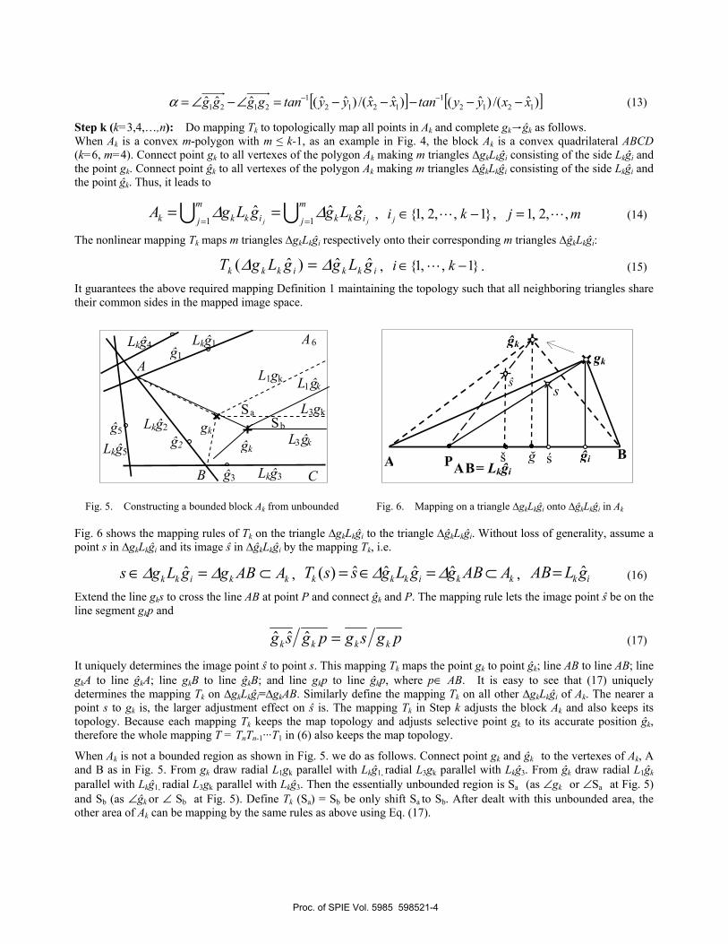
Step k (k=3,4,…,n): Do mapping Tk to topologically map all points in Ak and complete gk→ĝk as follows. When Ak is a convex m-polygon with m ≤ k-1, as an example in Fig. 4, the block Ak is a convex quadrilateral ABCD (k=6, m=4). Connect point gk to all vertexes of the polygon Ak making m triangles ∆gkLkĝi consisting of the side Lkĝi and the point gk. Connect point ĝk to all vertexes of the polygon Ak making m triangles ∆ĝkLkĝi consisting of the side Lkĝi and the point ĝk. Thus, it leads to

UUm

j ikkm

j ikkk jjgLggLgA

11ˆˆˆ

==== ∆∆ , }1,,2,1{ −∈ ki j L , mj ,,2,1 L= (14)

The nonlinear mapping Tk maps m triangles ∆gkLkĝi respectively onto their corresponding m triangles ∆ĝkLkĝi:

ikkikkk gLggLgT ˆˆ)ˆ( ∆∆ = , }1,,1{ −∈ ki L . (15) It guarantees the above required mapping Definition 1 maintaining the topology such that all neighboring triangles share their common sides in the mapped image space.

Fig. 5. Constructing a bounded block Ak from unbounded Fig. 6. Mapping on a triangle ∆gkLkĝi onto ∆ĝkLkĝi in Ak

Fig. 6 shows the mapping rules of Tk on the triangle ∆gkLkĝi to the triangle ∆ĝkLkĝi. Without loss of generality, assume a point s in ∆gkLkĝi and its image ŝ in ∆ĝkLkĝi by the mapping Tk, i.e.

kkikk AABggLgs ⊂=∈ ∆∆ ˆ , kkikkk AABggLgssT ⊂=∈= ˆˆˆˆ)( ∆∆ , ik gLAB ˆ= (16) Extend the line gks to cross the line AB at point P and connect ĝk and P. The mapping rule lets the image point ŝ be on the line segment gkp and

pgsgpgsg kkkk =ˆˆˆ (17)

It uniquely determines the image point ŝ to point s. This mapping Tk maps the point gk to point ĝk; line AB to line AB; line gkA to line ĝkA; line gkB to line ĝkB; and line gkp to line ĝkp, where p∈ AB. It is easy to see that (17) uniquely determines the mapping Tk on ∆gkLkĝi=∆gkAB. Similarly define the mapping Tk on all other ∆gkLkĝi of Ak. The nearer a point s to gk is, the larger adjustment effect on ŝ is. The mapping Tk in Step k adjusts the block Ak and also keeps its topology. Because each mapping Tk keeps the map topology and adjusts selective point gk to its accurate position ĝk, therefore the whole mapping T = TnTn-1···T1 in (6) also keeps the map topology.

When Ak is not a bounded region as shown in Fig. 5. we do as follows. Connect point gk and ĝk to the vertexes of Ak, A and B as in Fig. 5. From gk draw radial L1gk parallel with Lkĝ1, radial L3gk parallel with Lkĝ3. From ĝk draw radial L1ĝk parallel with Lkĝ1, radial L3gk parallel with Lkĝ3. Then the essentially unbounded region is Sa (as ∠gk or ∠Sa at Fig. 5)

and Sb (as ∠ĝk or ∠ Sb at Fig. 5). Define Tk (Sa) = Sb be only shift Sa to Sb. After dealt with this unbounded area, the other area of Ak can be mapping by the same rules as above using Eq. (17).

ĝ2

ĝ3 Lkĝ3

gk

ĝ1

ĝ5

1

Lkĝ5 ĝk

Lkĝ1

Lkĝ2

Lkĝ4 A6

Sa Sb

B

A

C

L1gk

L3gk

L1 ĝk

L3 ĝk

Bğ ĝi AB= Lkĝi A P

ĝk

ŝ s

gk

ś š

Proc. of SPIE Vol. 5985 598521-4

4. EXAMPLE This section shows an example to apply the new approaches to effective generation of a vector map and especially accurate adjustment of the vector map for Chengdu city. Fig. 1 is the vector map before adjusting, while Fig. 7 is this vector map after adjusting via the new method on 4 points. Fig. 8 is the map after 8 points adjusting. In those figures, the points marked by “+” are correct points ĝi, and the points marked by “×” are their corresponding points gk before adjusting on the vector map. More examples are also available at gps.ustc.edu.cn.

Fig. 7. Chengdu map after adjusting via 4 points Fig. 8. Chengdu map after adjusting via 8 points

ACKNOWLEDGEMENTS This work is supported by the National Natural Science Foundation of China under Grant Number 60272040.

REFERENCES

1. Li Deren. The digital earth and 3S Technology. Forum for GIS, 2001. Available: http://www.gischina.com. 2. Yuanlu Bao and Sheng-Guo Wang, “USTC GPS Intelligent Vehicle Navigation System”. Proceedings of 2001

International Symposium on Adaptive and Intelligent Systems and Control, Session VI-01, Charlottesville, VA, USA，June 25, 2001.

3. Bao Yuanlu, Xia Bing, et al. “Three key techniques on exploitation of GPS vehicle monitoring systems”. China Highway – Transportation Information Industry, Vol.2(3), pp.42–44, 2001.

4. Ding Bin, Wong Kok Cheong. “A System for automatic extraction of road network from maps”, in Proc. IEEE International Joint Symposia on Intelligence and Systems, Rockville, USA. pp.359–366, 1998.

5. Sheng-Guo Wang and Yuanlu Bao, “New intelligent method to generate vector maps for GPS navigation”, IFAC World Congress b'02, Barcelona. Paper 157, July 2002. Available: ifac2002.dit.upm.es/ifac2002/

6. Guo Jiehua, Yao Zhenwang, Bao Yuanlu and Zhang Wangsheng. “An auto-proofreading algorithm of geographic vector map”. Chinese Journal of Image and Graphics, Vol.4(5), pp.423–426, 1999.

7. Pu Baoming, Jiang Jiguang, Hu Shuli, Topology, Higher Education Press, Beijing, 1985.

Proc. of SPIE Vol. 5985 598521-5