an algorithm for automatic 2d quadrilateral mesh ... triangle...an algorithm for automatic 2d...
TRANSCRIPT

An algorithm for automatic 2D quadrilateral mesh generation
with line constraints
Kyu-Yeul Leea, In-Il Kimb, Doo-Yeoun Choc, Tae-wan Kimd,*
aDepartment of Naval Architecture and Ocean Engineering, Research Institute of Marine Systems Engineering, Seoul National University, San 56-1,
Shinlim-Dong, Kwanak-Gu, Seoul 151-742, South KoreabDaewoo Shipbuilding and Marine Engineering Co. Ltd, Ajoo-Dong, Koeje 656-714, South Korea
cDepartment of Naval Architecture and Ocean Engineering, Seoul National University, San 56-1, Shinlim-Dong, Kwanak-Gu, Seoul 151-742, South KoreadSeoul National University, Department of Naval Architecture and Ocean Engineering, Seoul 151-742, Korea
Abstract
Finite element method (FEM) is a fundamental numerical analysis technique widely used in engineering applications. Although state-of-
the-art hardware has reduced the solving time, which accounts for a small portion of the overall FEM analysis time, the relative time needed
to build mesh models has been increasing. In particular, mesh models that must model stiffeners, those features that are attached to the plate
in a ship structure, are imposed with line constraints and other constraints such as holes. To automatically generate a 2D quadrilateral mesh
with the line constraints, an extended algorithm to handle line constraints is proposed based on the constrained Delaunay triangulation and Q-
Morph algorithm. The performance of the proposed algorithm is evaluated, and numerical results of our proposed algorithm are presented.
q 2003 Elsevier Ltd. All rights reserved.
Keywords: Mesh Generation; Quadrilateral; Planar Meshing; Finite element method; Line constraint
1. Introduction
The finite element method (FEM) is one of the most
powerful analysis tools available in engineering. However,
one of the biggest obstacles that must be overcome for FEM
analysis to be used is the discretization of an arbitrary
geometry into a valid finite element mesh without user
interaction. Hence, automatic generation of finite element
mesh has been an important issue in today’s engineering
environment. In engineering applications, a triangle mesh
and a quadrilateral mesh are commonly used for 2D finite
element analysis. Quadrilateral mesh in general has better
quality and converges faster than the triangular mesh, but it is
more difficult to automatically generate a quadrilateral mesh
than a triangle mesh.
Most researches on the automatic generation of a 2D
quadrilateral mesh focus on the analysis domain with closed
boundary, as shown in Fig. 1. However, structures in some
engineering fields, such as ship production or airplane
production, have specific features such as stiffener attached
on the plate for reinforcement. In such a case, stiffener is
regarded as a line constraint that must be imposed on mesh, as
shown in Fig. 1. To automatically generate a quadrilateral
mesh with these line constraints, closed boundary as well as
open boundary made by line constraint must be resolved.
2. Related works
Quadrilateral mesh generators can be broadly classified
into two main categories: direct and indirect approaches,
according to the method employed to generate the
quadrilateral elements [1]. The direct approach places the
quadrilaterals on the domain directly without triangulation;
the indirect approach generates quadrilaterals by combin-
ing or splitting the background triangle mesh. The direct
approach can generally produce better quality meshes than
the indirect approach. However, the algorithms of the
direct approach are difficult to handle and implement, in
general [2].
2.1. Direct approach
Two main types of direct approach exist. The first
type, known as geometry decomposition, is a form of
0010-4485/03/$ - see front matter q 2003 Elsevier Ltd. All rights reserved.
doi:10.1016/S0010-4485(02)00145-8
Computer-Aided Design 35 (2003) 1055–1068
www.elsevier.com/locate/cad
* Corresponding author.
E-mail addresses: [email protected] (T. Kim), [email protected].
ac.kr (K. Y. Lee), [email protected] (I. I. Kim), [email protected]
(D. Y. Cho).

decomposition, which decomposes a domain into simpler,
convex, or mappable regions. Geometry decomposition can
be achieved by various techniques. Chae and Jeong [2],
Talbert and Parkinson [3], and Nowottny [4] used the
recursive decomposition algorithm. Baehmann et al. [5]
employed quad-tree decomposition technique for quad-
rilateral meshing. Tom and Amstrong [6] proposed a
technique us ing medial axis. Joe [7] utilizes decomposition
algorithms to decompose the area into convex polygons. In
general, though these methods generate an all-quad, high
quality mesh, they are difficult to automate, especially if a
domain with line constraint is involved.
The second method is advancing front methods to
form elements, one of which is known as Paving,
proposed by Blacker and Stepheson [8]. Paving forms
quadrilaterals starting from the boundary and working
inward. It generates a high quality mesh for a complex
arbitrary geometry. White and Kinney [9] suggested an
enhancement to the paving algorithm. However, paving
has some disadvantages as shown in Fig. 2, one of which
is an intersection problem by interference of opposing
elements. This problem intensifies if line constraints are
imposed on the domain. The other problem is the large
difference in element size between opposing fronts in
such instance, the paving algorithm to generate a poor
quality mesh. Because of these drawbacks, paving is
not suitable for generating quadrilateral with line
constraints.
2.2. Indirect approach
An indirect approach forms the quadrilateral using the
splitting triangle method or combining triangle method. The
splitting triangle method divides all triangles into three
quadrilaterals. This method guarantees an all-quadrilateral
mesh, but a high number of irregular nodes are introduced
into the mesh, resulting in poor quality. The combining
triangle method combines adjacent pairs of triangles to form
a single quadrilateral. Johnston et al. [10] and Lo and Lee [11]
used the combining triangle method. Although the combin-
ing triangle method generates elements whose quality is
better than those generated by the splitting triangle method,
the former method leaves a large number of triangles,
resulting in a mesh that is generally not as good quality as the
one generated by the direct approach.
The Q-Morph algorithm, which was recently introduced
by Owen et al. [12], utilizes an advancing front approach to
combine triangles into quadrilaterals. This algorithm can
generate better quality mesh than existing algorithms do. Q-
Morph algorithm can generate a quadrilateral mesh with
closed boundary only. However, applying this algorithm to
the generation of the quadrilateral mesh with the line
constraints would be more beneficial than direct approach
in terms of satisfying line constraints. The reasons are as
follows.
Advancing front direct approach must check globally
whether advancing front elements intersect each other or
not (see Fig. 2(a)), but this global intersection check is
not required in Q-Morph algorithm, because Q-Morph
algorithm only uses the edge information of input
triangular meshes to generate quadrilateral meshes.
More details of Q-Morph algorithm are explained in
Section 5.1.
3. Outline of the proposed mesh generation algorithm
To automatically generate a 2D quadrilateral mesh with
the line constraints, an extended algorithm to handle line
constraints is proposed based on the constrained Delaunay
triangulation (CDT) and Q-Morph algorithm. Fig. 3 shows
an outline of the proposed quadrilateral mesh generation
Fig. 1. Difference between closed boundary and open boundary.
Fig. 2. Drawbacks of paving method (a) interference of opposing elements (b) element size difference between opposing fronts.
K.-Y. Lee et al. / Computer-Aided Design 35 (2003) 1055–10681056

algorithm, and Table 1 shows the difference between the
proposed algorithm and Q-Morph.
4. Triangulation
Triangulation is a pre-requisite step to generating a
quadrilateral mesh by the indirect approach. Information,
such as shape or topology, obtained by triangulation offers
information on the mesh size as well as on the constraints of
quadrilateral meshing. In addition, the quality of the
triangulation influences the quality of the quadrilateral mesh.
4.1. Constrained Delaunay triangulation
The constraint in mesh generation requires the edges of
the final mesh pass through all the lines and points, selected
according to the users’ needs. The CDT can be used to
generate a triangle mesh satisfying the line constraints.
Delaunay triangulation is an efficient domain
decomposition technique widely used in computational
geometry. In Delaunay triangulation, an arbitrary triangle
set is obtained using the order of point insertion and distance
between points [13,14]. However, Delaunay triangulation
alone cannot generate a triangle mesh satisfying line
constraints. To resolve this problem, that is, to generate a
triangle mesh satisfying line constraints, a CDT [15,16] is
used in this study. This algorithm examines all edges of all
triangle meshes. If the edge, imposed as a line constraint, is
not included in the resulting mesh, the algorithm inserts the
edge and then re-triangulates the domain around the inserted
edge. In doing so, this algorithm preserves the edges imposed
as line constraints. Fig. 4(a) shows the CDT. Bold lines show
external and internal boundaries (closed boundary) and
dashed lines show the line constraints (open boundary). The
domain is triangulated satisfying the line constraints in
Fig. 4(a) and this can be verified.
4.2. Field point generation to get desired triangle mesh size
The triangle meshes with line constraints can be generated
by CDT. However, this mesh contains boundary points only
(Fig. 4(a)), and thus is generally inappropriate for numerical
computation and does not reflect the user’s needs in terms of
mesh size. Therefore, internal points must be created and
inserted in the mesh domain generated by the CDT,
according to the desired size of the mesh. The quality of
the quadrilateral mesh is highly dependent on the quality of
triangle mesh, and because the shape and topology of the
triangle mesh depends on the position of the insertion points,
it is important that the internal points are inserted at proper
positions.
In this study, a field point generation method which does
not destroy the given line constraints and can be manipulated
to generate a mesh of a desired size, while preserving a near-
regular triangle mesh, is studied and implemented.
Borouchaki and George [17,18] and Ruppert [19] points
Fig. 3. Outline of the proposed mesh generation algorithm can satisfy line constraints (dashed box indicates the proposed algorithm).
Table 1
Comparison of proposed algorithm with Q-Morph
Q-Morph
algorithm
Proposed
algorithm
Quad algorithm Indirect method,
advancing
front approach
Indirect method
advancing
front approach
Closed boundary (hole, outer
boundary)
O O
Open boundary (line constraint) X O
K.-Y. Lee et al. / Computer-Aided Design 35 (2003) 1055–1068 1057

insertion algorithms are existing methods. But, Ruppert’s
algorithm is not suitable for our purposes because sometimes
the points are inserted on the edges, imposed as line
constraints; hence, the Borouchaki and George’s points
insertion algorithm is selected for study and included in the
implementation.
Borouchaki and George’s points insertion algorithm uses
a ‘local parameter h’, which is defined as the desirable
distance between any point and its neighbor on the same
boundary, which includes external boundaries and line
constraints. Based on this parameter, insertion points are
generated by subdividing the edges belonging to all triangles,
excluding the line constraints, and then the generated points
are inserted into the mesh domain by Delaunay triangulation.
Fig. 4(b) shows a triangle mesh with three points inserted.
Fig. 4(c) shows the final triangle mesh with all generated
points inserted.
5. Quadrilateral meshing
5.1. Q-Morph algorithm
The Q-Morph algorithm is an indirect approach used
to form a quadrilateral mesh from a pre-formed
background triangle mesh. While it is similar to the
existing indirect approaches, in that it forms a quad-
rilateral mesh by combining background triangles, this
method improves on the mesh quality by using an
advancing front approach, used in paving, to convert
triangles to quads. Fig. 5 shows the transformation of a
triangle mesh to a quadrilateral mesh as the boundary of
the mesh domain proceeds. The boundary of a mesh
domain is called the front edge, which is defined as the
set of edges that comes in contact with a single triangle
and is a subset of all edges belonging to all triangles.
Fig. 6 is a flow diagram of the Q-Morph algorithm. The
starting set of front edges is selected from the initial triangle
mesh. A quadrilateral mesh is formed by merging triangles
from selected front edges, after which the state of the front
edge is updated. This process is iterated until no single front
edge exists. If there are no more front edges, the merging
process is complete. After the quadrilateral mesh generation
process completes, the cleanup and smoothing process are
performed to improve mesh quality.
The box on the right in Fig. 6 lists the procedures to
forming a quadrilateral mesh by merging background
triangle meshes. Whenever any number of triangles merges
to form a single quadrilateral, the steps between the front
Fig. 4. Procedure of triangle mesh generation satisfying line constraint. (a) CDT, (b) triangle mesh after inserting three field points in the mesh domain
generated by CDT, (c) final triangle mesh after inserting all field points (dashed line indicates the line constraint).
Fig. 5. Procedure of Q-Morph algorithm [12] (bold line indicates front edge proceeding by mesh generation procedure).
K.-Y. Lee et al. / Computer-Aided Design 35 (2003) 1055–10681058

edge classification step and the local smoothing step are
repeated. Details of the process are briefly outlined in the
following steps
1. Front edge classification and front edge sorting: classify-
ing the current state of the front and sorting.
2. Side edge definition: generating the side edges of a
quadrilateral.
3. Top edge recovery: generating the top edge of a
quadrilateral.
4. Quadrilateral formation: forming a quadrilateral with
edges generated by step (2) and step (3).
5. Local smoothing: local improvement of mesh quality.
6. Closing the front: when opposing fronts meet, fronts are
merged to define a continuous mesh.
Fig. 7 shows the procedure of forming a single
quadrilateral by merging triangles.
5.2. Proposed algorithm for handling line constraints
The Q-Morph algorithm, as described in Section 5.1, is an
algorithm for domains with closed boundaries. But our
objective is to generate quadrilateral meshes with not only
closed boundaries but also open boundaries. The dashed line
of Fig. 4 shows open boundaries, such as line constraints.
To generate quadrilaterals with open boundaries, an
extended Q-Morph algorithm is proposed. Fig. 8 shows the
procedure of the proposed algorithm and Algorithm 1 shows
the pseudo-code of the proposed algorithm. In Algorithm 1,
seam is the operation performed if the angle between two
adjacent edges on the front is small. The seaming criterion
determined by heuristic manner is p/6. Quadrilateral meshes
satisfying line constraints can be generated by improving
edge classification and side edge definition steps in the Q-
Morph algorithm.
The front edge is defined as the set of edges that comes in
contact with a single triangle and is a subset of all edges
belonging to all triangles. If one examines the front edge
proceeding from the internal and external boundaries in
Fig. 5, one can verify that the front edge comes in contact
with a single triangle in every case. The Q-Morph algorithm
classifies the state of front edges into four cases in its front
Fig. 6. Flow diagram of Q-Morph algorithm.
Fig. 7. Procedure of forming a quadrilateral by Q-Morph algorithm [12].
K.-Y. Lee et al. / Computer-Aided Design 35 (2003) 1055–1068 1059

edge classification step, as shown in Fig. 9. State 0 represents
the case where a side edge is made by searching a
neighboring triangle, and state 1 represents the case where
the adjacent front edge is defined as the side edge. Here, one
can verify that any single front edge always links up with
another front edge. With only closed boundaries in a domain,
the end of any single front edge always links up with another
front edge.
However, when the edges imposed as line constraints
are examined, it becomes apparent that this is the same
Fig. 8. Procedure of the proposed algorithm: improvement of edge classification and side edge definition steps for handling line constraints (bold box indicates
the proposed part).
Algorithm 1. Pseudo-code of proposed algorithm (the parts pointed by the bold arrows are proposed parts).
K.-Y. Lee et al. / Computer-Aided Design 35 (2003) 1055–10681060
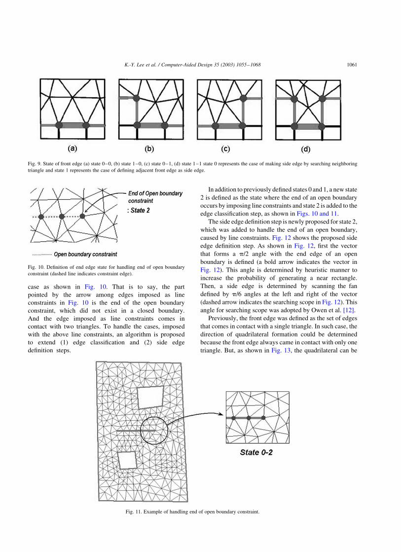
case as shown in Fig. 10. That is to say, the part
pointed by the arrow among edges imposed as line
constraints in Fig. 10 is the end of the open boundary
constraint, which did not exist in a closed boundary.
And the edge imposed as line constraints comes in
contact with two triangles. To handle the cases, imposed
with the above line constraints, an algorithm is proposed
to extend (1) edge classification and (2) side edge
definition steps.
In addition to previously defined states 0 and 1, a new state
2 is defined as the state where the end of an open boundary
occurs by imposing line constraints and state 2 is added to the
edge classification step, as shown in Figs. 10 and 11.
The side edge definition step is newly proposed for state 2,
which was added to handle the end of an open boundary,
caused by line constraints. Fig. 12 shows the proposed side
edge definition step. As shown in Fig. 12, first the vector
that forms a p/2 angle with the end edge of an open
boundary is defined (a bold arrow indicates the vector in
Fig. 12). This angle is determined by heuristic manner to
increase the probability of generating a near rectangle.
Then, a side edge is determined by scanning the fan
defined by p/6 angles at the left and right of the vector
(dashed arrow indicates the searching scope in Fig. 12). This
angle for searching scope was adopted by Owen et al. [12].
Previously, the front edge was defined as the set of edges
that comes in contact with a single triangle. In such case, the
direction of quadrilateral formation could be determined
because the front edge always came in contact with only one
triangle. But, as shown in Fig. 13, the quadrilateral can be
Fig. 9. State of front edge (a) state 0–0, (b) state 1–0, (c) state 0–1, (d) state 1–1 state 0 represents the case of making side edge by searching neighboring
triangle and state 1 represents the case of defining adjacent front edge as side edge.
Fig. 10. Definition of end edge state for handling end of open boundary
constraint (dashed line indicates constraint edge).
Fig. 11. Example of handling end of open boundary constraint.
K.-Y. Lee et al. / Computer-Aided Design 35 (2003) 1055–1068 1061

formed in two directions because an edge, imposed as a line
constraint, comes in contact with two triangles. Hence, the
direction of quadrilateral formation must be determined. In
our work, the direction of quadrilateral formation is fixed to
one particular direction, as shown in Fig. 13, so that the open
boundary, incurred by line constraints, can be transformed
into a closed boundary such as a hole.
5.3. Preventing triangle from remaining
Quadrilaterals are formed by merging triangles as the
front proceeds, but some triangles may not merge with
others. Such a case is shown in Fig. 14, where the number of
front edges belonging to the front loop is odd. A front loop is
defined as all the edges on the front comprising a continuous
unbroken ring. Any number of loops may be active at a given
time in number throughout the entire process of meshing so
that no single triangle is left out. To maintain all loops as
even, the process of meshing. Fig. 14 shows two loops. If an
odd loop is generated, some triangles do not merge with
exception. Therefore, the number of edges belonging to a
front loop must be maintained as an even potential number of
front edges on the new loop to be formed is first determined at
the moment opposing fronts encounter each other. If the
potential number of front edges is even, then the front is
merged and a new loop is defined. If the potential number of
front edges is odd, then the front is not merged but side edges
are split, as shown in Fig. 15. With this method, every newly
Fig. 12. Side edge definition for end of open boundary constraint.
Fig. 13. Example of merging triangles with same direction and status of constraints and front edge.
K.-Y. Lee et al. / Computer-Aided Design 35 (2003) 1055–10681062

formed loop is given an even number of edges, thereby
precluding any possibility of remaining triangles.
6. Mesh smoothing
A constrained Laplacian smoothing algorithm is iterated
for mesh smoothing. Constrained Laplacian smoothing is a
method where each node is moved to the centroid of its
neighbors only if it improves element quality. If an
element’s quality is not expected to improve, the node is
not moved. The overall quality of the mesh is evaluated by
the average distortion coefficient ð �bÞ described by Lo and
Lee [11]. The average distortion coefficient ð �bÞ is the
geometrical mean of the distortion coefficient (b ) values of
the quadrilaterals. b for the quadrilateral ABCD can be
defined as follows
b¼a3a4
a1a2
where{a1;a2;a1;a2}¼{aðABCÞ;aðACDÞ;aðABDÞ;aðBCDÞ}
a1$a2$a1$a2 ð1Þ
8<:
Fig. 14. Case of triangles remaining.
Fig. 15. Splitting side edge to maintain even loop for preventing triangle from remaining (dashed box indicates example of splitting side edge: bold edge is split).
K.-Y. Lee et al. / Computer-Aided Design 35 (2003) 1055–1068 1063

where a is defined as follows
aðABCÞ¼2ffiffi3
p kCA£CBkkCAk2þkABk2þkBCk2
ð2Þ
For rectangles, b attains a maximum value of 1, whereas
for quadrilaterals degenerated to triangles, b approaches 0.
The criterion for mesh quality adopted by Lo and Lee [11]
is given in Table 2.
7. Mesh example
Four example problems, shown in Figs. 16–19, demon-
strate various features of the proposed algorithm.
The first example, shown in Fig. 16, shows the result of
applying the proposed algorithm to a simple model with two
holes and one line constraint. CDT, implemented in this
study, is used to create the triangles. Fig. 16(a) shows the
front, proceeding forward one layer and Fig. 16(b) shows the
front proceeding while forming quadrilaterals. Fig. 16(c)
shows a completed quadrilateral mesh generation and
Fig. 16(d) shows the shape of a quadrilateral mesh after
Table 2
Mesh quality criteria using average distortion coefficient
Value of �b Description
�b , 0:36 Unacceptable
0:36 # �b , 0:54 Marginal, but acceptable
0:54 # �b , 0:72 Good�b $ 0:72 Excellent
Fig. 16. Application of the proposed algorithm to simple model with two holes and one line constraint: (a) and (b) forming quadrilateral (c) before smoothing
(d) after smoothing (dashed line indicates constraint).
K.-Y. Lee et al. / Computer-Aided Design 35 (2003) 1055–10681064

smoothing. Fig. 16 shows that the generated quadrilateral
mesh satisfies the line constraints perfectly. The quantitative
evaluation of the quadrilateral mesh by average distortion
coefficient ð �bÞ is shown in Table 3 located at the end of
this chapter.
Fig. 17 is an example of applying the proposed algorithm
to Owen’s model (Fig. 5). An advancing front triangle
mesher is used to create the triangles, as Owen did. Fig. 17(a)
shows a background triangle mesh; Fig. 17(b) shows the
quadrilateral meshes after generation is completed; and
Fig. 18. Application of the proposed algorithm to a more complicated model with one hole and six line constraints. (a) and (b) forming quadrilateral (c) before
smoothing (d) after smoothing (dashed line indicates constraint).
Fig. 17. Application of applying the proposed algorithm to Owen [3] model (Fig. 5): (a) initial triangulation (b) before smoothing (c) after smoothing.
K.-Y. Lee et al. / Computer-Aided Design 35 (2003) 1055–1068 1065

Fig. 17(c) shows the shape of the quadrilateral mesh after
smoothing. The final shape of the quadrilateral mesh is
slightly different from that of Owen’s (Fig. 5) because of the
differences in the triangle meshes used. The high quality of
the shape of the quadrilateral mesh can be verified.
The quantitative evaluation of the quadrilateral mesh by
average distortion coefficient ð �bÞ is shown in Table 3 located
at the end of this chapter.
Fig. 18 is an example of applying the proposed algorithm
to a more complicated model with one hole and six line
constraints. CDT, implemented in this study, is used to create
the triangles. This example shows that the proposed
algorithm can be applied to models with any number of
line constraints. Fig. 18(a) shows the front proceeding
forward one layer and Fig. 18(b) shows the front proceeding
while forming quadrilaterals. Fig. 18(c) shows the quad-
rilateral mesh after generation is completed and Fig. 18(d)
shows the shape of the quadrilateral mesh after smoothing.
As shown in Fig. 18, the generated quadrilateral mesh
satisfies the line constraints perfectly. The quantitative
evaluation of the quadrilateral mesh by average distortion
coefficient ð �bÞ is shown in Table 3 located at the end of this
chapter.
Fig. 19 is an example of applying the proposed algorithm
to a ship structure model, specifically a transverse bulkhead
with full boundary shape and simplified line constraints for
testing. CDT, implemented in this study, is used to create the
triangles. Though this model has very complex internal and
external boundaries, a quadrilateral mesh satisfying these
boundaries and line constraints can be generated by the
proposed algorithm. The quantitative evaluation of the
quadrilateral mesh by average distortion coefficient ð �bÞ is
shown in Table 3 located at the end of this chapter.
Table 3
Average distortion coefficient of the examples in Figs.16–19
Model Before smoothing After smoothing
Fig. 16 0.533969 0.654108
Fig. 17 0.562550 0.736361
Fig. 18 0.523413 0.721393
Fig. 19 0.416651 0.65
Fig. 19. Application of applying the proposed algorithm to ship structure model (transverse bulkhead with full boundary shape and simplified line constraints
for testing), (a) and (b) forming quadrilateral, (c) before smoothing (d) after smoothing (dashed line indicates constraint).
K.-Y. Lee et al. / Computer-Aided Design 35 (2003) 1055–10681066
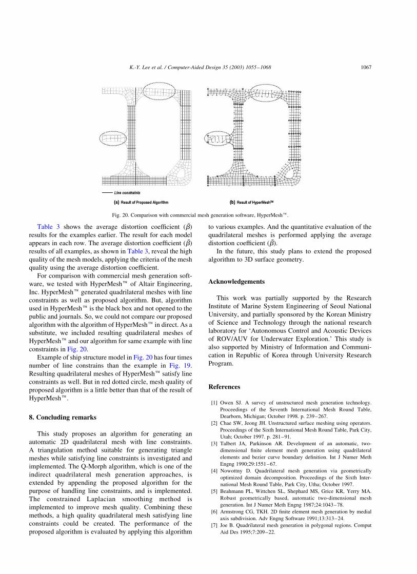
Table 3 shows the average distortion coefficient ð �bÞ
results for the examples earlier. The result for each model
appears in each row. The average distortion coefficient ð �bÞ
results of all examples, as shown in Table 3, reveal the high
quality of the mesh models, applying the criteria of the mesh
quality using the average distortion coefficient.
For comparison with commercial mesh generation soft-
ware, we tested with HyperMeshe of Altair Engineering,
Inc. HyperMeshe generated quadrilateral meshes with line
constraints as well as proposed algorithm. But, algorithm
used in HyperMeshe is the black box and not opened to the
public and journals. So, we could not compare our proposed
algorithm with the algorithm of HyperMeshe in direct. As a
substitute, we included resulting quadrilateral meshes of
HyperMeshe and our algorithm for same example with line
constraints in Fig. 20.
Example of ship structure model in Fig. 20 has four times
number of line constrains than the example in Fig. 19.
Resulting quadrilateral meshes of HyperMeshe satisfy line
constraints as well. But in red dotted circle, mesh quality of
proposed algorithm is a little better than that of the result of
HyperMeshe.
8. Concluding remarks
This study proposes an algorithm for generating an
automatic 2D quadrilateral mesh with line constraints.
A triangulation method suitable for generating triangle
meshes while satisfying line constraints is investigated and
implemented. The Q-Morph algorithm, which is one of the
indirect quadrilateral mesh generation approaches, is
extended by appending the proposed algorithm for the
purpose of handling line constraints, and is implemented.
The constrained Laplacian smoothing method is
implemented to improve mesh quality. Combining these
methods, a high quality quadrilateral mesh satisfying line
constraints could be created. The performance of the
proposed algorithm is evaluated by applying this algorithm
to various examples. And the quantitative evaluation of the
quadrilateral meshes is performed applying the average
distortion coefficient ð �bÞ:
In the future, this study plans to extend the proposed
algorithm to 3D surface geometry.
Acknowledgements
This work was partially supported by the Research
Institute of Marine System Engineering of Seoul National
University, and partially sponsored by the Korean Ministry
of Science and Technology through the national research
laboratory for ‘Autonomous Control and Acoustic Devices
of ROV/AUV for Underwater Exploration.’ This study is
also supported by Ministry of Information and Communi-
cation in Republic of Korea through University Research
Program.
References
[1] Owen SJ. A survey of unstructured mesh generation technology.
Proceedings of the Seventh International Mesh Round Table,
Dearborn, Michigan; October 1998. p. 239–267.
[2] Chae SW, Jeong JH. Unstructured surface meshing using operators.
Proceedings of the Sixth International Mesh Round Table, Park City,
Utah; October 1997. p. 281–91.
[3] Talbert JA, Parkinson AR. Development of an automatic, two-
dimensional finite element mesh generation using quadrilateral
elements and bezier curve boundary definition. Int J Numer Meth
Engng 1990;29:1551–67.
[4] Nowottny D. Quadrilateral mesh generation via geometrically
optimized domain decomposition. Proceedings of the Sixth Inter-
national Mesh Round Table, Park City, Utha; October 1997.
[5] Beahmann PL, Wittchen SL, Shephard MS, Grice KR, Yerry MA.
Robust geometrically based, automatic two-dimensional mesh
generation. Int J Numer Meth Engng 1987;24:1043–78.
[6] Armstrong CG, TKH. 2D finite element mesh generation by medial
axis subdivision. Adv Engng Software 1991;13:313–24.
[7] Joe B. Quadrilateral mesh generation in polygonal regions. Comput
Aid Des 1995;7:209–22.
Fig. 20. Comparison with commercial mesh generation software, HyperMeshe.
K.-Y. Lee et al. / Computer-Aided Design 35 (2003) 1055–1068 1067

[8] Blacker TD, Stephenson MB. Paving: a new approach to automated
quadrilateral mesh generation. Int J Numer Meth Engng 1991;32:
811–47.
[9] White DR, Kinney P. Redesign of the paving algorithm: robustness
enhancements through element by element meshing. Proceedings of
the Sixth International Mesh Round Table, Park City, Utha; October
1997. p. 323–35.
[10] Johnston BP, Sullivan Jr. JM, Kwasnik A. Automatic conversion of
triangular finite element meshes to quadrilateral elements. Int J Numer
Meth Engng 1991;31:67–84.
[11] Lee CK, Lo SH. A new scheme for the generation of a graded
quadrilateral mesh. Comput Struct 1994;52(5):847–57.
[12] Owen SJ, Staten ML, Canann SA, Saigal S. Q-Morph: an indirect
approach to advancing front quad meshing. Int J Numer Meth Engng
1999;44:1317–40.
[13] de Berg M, van Kreveld M, Overmars M. Computational geometry:
algorithms and applications. Berlin: Springer; 1997.
[14] George PL. Automatic mesh generation application to finite element
methods. New York: Wiley; 1991.
[15] Chew LP. Constrained Delaunay triangulation. Comput Geometr
Symp, ACM 1987;215–22.
[16] Shewchuk JR. Triangle: engineering a 2D mesh generator and
Delaunay triangulator. First Workshop on Applied Computational
Geometry, ACM; 1996.
[17] Borouchaki H, George PL. Aspects of 2-D Delaunay mesh generation.
Int J Numer Meth Engng 1997;40:1957–75.
[18] Borouchaki H, George PL, Lo SH. Optimal Delaunay point insertion.
Int J Numer Meth Engng 1996;39:3407–37.
[19] Ruppert J. A Delaunay refinement algorithm for quality 2-dimensional
mesh generation. J Algorithm 1995;18(3):548–85.
Kyu-Yeul Lee is Professor in the Department
of Naval Architecture and Ocean Engineering
and the Research Institute of Marine System
Engineering at Seoul National University,
Seoul, Korea. His research interests are in the
areas of geometric modeling, design auto-
mation, optimization, and CAD in shipbuild-
ing. He was the project leader of the korean
national research project ‘Computerized Ship
Design and Production System’. He received
his BS in 1971 from the Seoul National
University, and his MS in 1975 and PhD in
1982 from the Technical University Hannover, Germany, all in the
Naval Architecture.
In-Il Kim is currently a Research Engineer at
Daewoo Shipbuilding and Marine Engineering
Co. Ltd, Korea. He received his BS in 2000
and MS in 2002 from the Seoul National
University in Naval Architecture and Ocean
Engineering. His research interests include
CAD, computational geometry, Mesh gener-
ation and CAD/CAE interface.
Doo-Yeoun Cho is a PhD student in the
Department of Naval Architecture and Ocean
Engineering at Seoul National University,
Korea. He received his BS in 1997 and MS
in 1999 from the Seoul National University in
Naval Architecture and Ocean Engineering.
His research interests include CAD/CAM,
geometric modeling, NURBS curves and
surfaces, computer graphics and web3d.
Tae-wan Kim is an Assistant Professor in the
Department of Naval Architecture and Ocean
Engineering and Research Institute of Marine
System Engineering at Seoul National Uni-
versity, Seoul, Korea. He received a BS in
Industrial Engineering from Hanyang Univer-
sity, Korea, an MS, and a PhD in Computer
Science from Arizona State University,
USA in 1985, 1993 and 1996,
respectively. From 1996 to 1999 he worked
as a software engineer at Structural Dynamics
Research Corporation, USA where he
was involved in developing I-DEAS CAD/CAM system. From 1999 to
2001 he worked as a post-doctoral researcher at National Research
Laboratory in Seoul National University, Korea. His research interests
include geometric modeling, NURBS curves and surfaces, 3D digital
watermarking, and digital contents.
K.-Y. Lee et al. / Computer-Aided Design 35 (2003) 1055–10681068