an agent-based model for collaborative learning - school of
TRANSCRIPT

An agent-based model
for collaborative learning
Xavier Rafael Palou
Master by Research
Artificial Intelligence
School of Informatics
University of Edinburgh
2008

ii
Abstract
This project focuses on the classification problem in distributed data mining environments where the
transfer of data between learning processes is limited. Existing solutions address this problem through
the use of distributed technologies for applying data mining algorithms to learn global models from
local learning processes. Multiagent based solutions that follow this approach overlook the autonomy
of local learning processes, the decentralisation of system control, and the local learning heterogeneity
of the processes.
We propose a collaborative agent-based learning model inspired by an existing learning framework
that overcomes these deficiencies by defining the overall learning process as a combination of local
autonomous learners interacting with each other in order to improve their local classification
performance. Our model is an extension of this work and redefines agent learning behaviour as
consisting of four distinct steps: the selection of the learner with which to interact, the integration of
acquired knowledge, the evaluation of the resulting model and the update of the learning knowledge.
For each of these different steps, several methods and criteria have been proposed in order to offer
different alternatives for configuring the collaborative learning algorithm for limited data sharing
domains.
Integration of knowledge among the learners is the key feature of our agent model as it defines what
knowledge the learners are able to use and how to use it. We propose the use of several methods based
on existing Machine Learning techniques for integrating predicted classes, estimated posterior
probabilities and small batches of training data. Furthermore, we define a new method for integrating
heterogeneous tree models where the model is itself modified during integration. This method
outperforms alternative methods such as ensemble learning or model combination without loss of
model interpretability.
We developed a test application to evaluate the different configurations of our collaborative agent
model. The results show that collaborative learning dramatically increases the classification accuracy
of local learning agents when compared with isolated distributed learning and in the long run achieves
almost the same performance as those solutions that use centralised data.

iii
Acknowledgements
First, I would like to thank my supervisor Dr. Michael Rovatsos, for his guidance, patience and for all
the feedback, discussions and advice that he has given me, without which, this work would not be
possible.
I am also very grateful to MicroArt, and in particular to Magi Lluch and Mariola Mier for offering me
the opportunity to conduct this research, and for their understanding and encouragement to conclude
this work.
I am indebted for all the feedback that I received from my colleagues within CISA, especially
Alexandros-Sotiris Belesiotis, Francesco Figari and Tommy French and particularly to George
Christelis. To all of them, thanks also for the great moments, talks, coffees, lunches that we have
shared. I would also like to thank the rest of my friends that I have met during my stay in Edinburgh,
including Pedro and Itxaso, but especially Maria who has always been there during the best and worst
moments. Without them I would not be able to survive and enjoy this unforgettable experience.
Finally, this work is dedicated especially to my sister, mother and father, their pure love is everything
to me.
My Msc by Research at Edinburgh was founded by a Marie Curie Transfer of Knowledge scholarship
(no. IST-2004-27214) for which I am deeply grateful.

iv
Declaration
I declare that this thesis was composed by myself, that the work contained herein is my own except
where explicitly stated otherwise in the text, and that this work has not been submitted for any other
degree or professional qualification except as specified.
(Xavier Rafael Palou)

v
Table of Contents
1. Introduction .........................................................................................................................................1
1.1 Motivation....................................................................................................................................1
1.2 Research approach........................................................................................................................2
1.3 Research objectives......................................................................................................................3
1.4 Research method...........................................................................................................................4
1.5 Structure of the dissertation..........................................................................................................5
2. Background..........................................................................................................................................6
2.1 Introduction..................................................................................................................................6
2.2 Multiagent systems.......................................................................................................................6
2.3 Multiagent systems for distributed data mining...........................................................................7
2.3.1 The classifier learning problem in distributed environments...............................................8
2.3.2 DDM solutions for learning classifiers..............................................................................9
2.3.3 Multiagent solutions for distributed classification............................................................12
2.4 Conclusions................................................................................................................................14
3. A collaborative agent-based learning model......................................................................................15
3.1 Introduction................................................................................................................................15
3.2 Distributed agent learning framework overview........................................................................16
3.3 Collaborative learning model.....................................................................................................20
3.4 Neighbour selection....................................................................................................................22
3.5 Knowledge integration ..............................................................................................................27
3.5.1 Data merging......................................................................................................................28
3.5.2 Merging outputs.................................................................................................................30
3.5.3 Hypothesis merging.................................................................................................................38
3.6 Performance evaluation..............................................................................................................42
3.7 Knowledge update......................................................................................................................42
3.8 Termination criterion..................................................................................................................43
3.9 Conclusions................................................................................................................................44
4. Implementation...................................................................................................................................45
4.1 Introduction................................................................................................................................45
4.2 Objectives of the implementation...............................................................................................45
4.3. Application architecture overview ............................................................................................46
4.4 Functional design of the application ..........................................................................................47
vi
4.4.1 Setup of the learning environment.....................................................................................48
4.4.2 Running the learning experiments.....................................................................................48
4.4.3 Preparation of the learning results.....................................................................................52
4.5 Implementation of the application..............................................................................................52
4.5.1 Class diagram.....................................................................................................................53
4.5.2 Implementation of the centralised learning strategy..........................................................54
4.5.3 Implementation of the distributed isolated learning strategy.............................................54
4.5.4 Implementation of the collaborative learning strategy......................................................55
4.6 Summary.....................................................................................................................................69
5. Evaluation ..........................................................................................................................................70
5.1. Introduction...............................................................................................................................70
5.2 Scenario setup ............................................................................................................................70
5.3 Learning experiment setup.........................................................................................................72
5.4 Experimental results ..................................................................................................................73
5.4.1 Homogeneous case.............................................................................................................73
5.4.2 Results for heterogeneous scenario....................................................................................76
5.5 Conclusions from the results......................................................................................................93
5.5.1 General aspects of different learning strategies.................................................................93
5.5.2 General aspects of collaborative learning..........................................................................93
6. Conclusions and further work............................................................................................................99
Bibliography.........................................................................................................................................101
vii
List of Tables
Table3. 1: Matrix of integration knowledge operations.........................................................................28
Table 3.2: Merging hypothesis method..................................................................................................40
Table 3.3: Main functionalities of tree merging technique.....................................................................41
Table 5. 4: List of datasets for the learning experiments........................................................................71
Table 5.5: Table of different scenarios for the experiments...................................................................72
Table 5.6: List of learning experiments configuration...........................................................................72
Table 5 7: Summary of results for the homogeneous case with a greedy accuracy-based strategy.......73
Table 5.8: Summary of results for heterogeneous environment with a greedy accuracy-based strategy
................................................................................................................................................................76
Table 5.9: Comparing heterogeneous and homogeneous learning.........................................................78
Table 5.10: Results for heterogeneous environment with a random weighted accuracy-based strategy
................................................................................................................................................................80
Table 5.11: Analysis of interactions of collaborative learning for all datasets in heterogeneous scenario
................................................................................................................................................................81
Table 5.12: Learning interactions information for Letter dataset...........................................................82
Table 5.13: Variations of accuracy when increasing the number of agents in the system.....................85
Table 5.14: Variation of accuracy when increasing training sets from 60% to 80% of all available data
................................................................................................................................................................88
Table 5.15: Time needed for all the learning methods in a heterogeneous scenario with greedy
accuracy-based neighbour selection strategy.........................................................................................89

viii
List of Figures
Fig. 3.1: Generic learning step...............................................................................................................16
Fig. 3. 2: Matrix of knowledge integration functions from learner j using learner i..............................18
Fig.3.3: Learning step of collaborative model of the agent...................................................................21
Fig.3. 4: FIPA Contract Net interaction protocol...................................................................................26
Fig3. 5: Schema for data merging process.............................................................................................28
Fig.3. 6: Data merging integration operation.........................................................................................29
Fig.3.7: Resulting separation curves from simple voting method applied to n predictors....................31
Fig.3.8: Schema for merging n classifier probabilities.........................................................................34
Fig.3.9: Dimension space of instances...................................................................................................36
Fig.3.10: Schema for merging n classifier distances to centroids .........................................................36
Fig.3.11: Output merging integration operation.....................................................................................38
Fig.3.12: Different scenarios based on different classification abilities................................................39
Fig4. 1: Execution flow of the application ............................................................................................47
Fig.4.2: Design of centralised learning for the heterogeneous scenario................................................50
Fig.4.3: Design of the distributed isolated learning in a heterogeneous environment..........................50
Fig.4.4: Design of the collaborative learning strategy for a heterogeneous environment.....................51
Fig.4.5: Application class diagram ........................................................................................................53
Fig.4. 6: Pseudo-code for centralised strategy.......................................................................................54
Fig.4. 7: Pseudo-code for distributed isolated strategy..........................................................................55
Fig.4. 8: Pseudo algorithm collaborative learning strategy....................................................................56
Fig.4. 9: WeightRandomizedNext method for the weighted randomised neighbour criterion..............58
Fig.4.10: Joining Data method for knowledge integration operation....................................................59
Fig.4. 11: Output merging method for knowledge integration operation...............................................59
Fig.4. 12: ColTree conversion of a base Weka classifier (SimpleCart)..................................................60
Fig.4.13: Method which returns a vector of ColBranches for a SimpleCart classifier..........................61
Fig.4. 14: Method for converting a single branch of a SimpleCart tree to a ColBranchTree................61
Fig.4. 15: Method for compacting a ColBranchTree.............................................................................62
Fig.4. 16: Method for merging ColTree classifiers................................................................................63
Fig.4. 17: Method for getting the branches of the ColTree classifier.....................................................64
Fig.4. 18: Method for cleaning up the branches of a set of colBranchTree classifiers.........................65
Fig.4. 19: Method for merging output classification..............................................................................66
Fig.4.20: Classification using the sum of class probabilities for different classifiers............................67
Fig.4.21: Classification using the tree merging method.........................................................................67

ix
Fig.4. 22: Method for calculating posterior class distributions for an instance of a ColBranchTree.....68
Fig.5.1: Comparison of the three learning strategies in a homogeneous scenario for different agent
configurations.........................................................................................................................................75
Fig. 5. 2: Accuracy v. interaction count in Letters dataset.....................................................................84
Fig. 5. 3: Comparison of different agent configurations.......................................................................86
Fig. 5.4: Comparison of learning method performance when size of training sets is increased............87
Fig. 5.5: Increase of accuracy over time for all datasets........................................................................92


Chapter 1 Introduction 1
Chapter 1
Introduction
1.1 Motivation
This dissertation focuses on the Data Mining research area and in particular it addresses classification
problems which involve a learning process used to obtain a predictive model from a set of data.
Usually this data is just a portion of all possible data, and the model therefore has to generalise as
much as possible in order to accurately classify unseen instances.
Traditionally, learning to classify is a centralised, off-line process. The data available is collected from
a central repository and the experts select and parametrise a machine learning algorithm in order to
obtain a predictive model over the available data.
Nowadays, however, distributed and open environments are a more common system configuration.
Therefore, the learning process is transformed into a distributed data mining problem where the data is
inherently distributed across several nodes of a network.
One of the most widely used approaches to the distributed data mining problem is to gather all the
data from the local nodes in a central repository and then apply traditional data mining techniques.
However, in several domains the exchange and sharing of data is not allowed or feasible. For example,
local data may change quickly, may be too complex or too costly to communicate, or it may not be
possible to reveal all information for reasons such as security, legal restrictions or competitive
advantage. More specific examples of this type of application can be found in the literature, like the
distributed medical care domain, where the use of sensitive data and the exchange of data is restricted
or prohibited (e.g. brain tumour classification [31]). In other, more business-oriented areas, training
data might be an economic asset to a company, which might not wish to share the data for free (e.g.
remote ship surveillance [35]). In other areas, datasets contain large amounts of distributed data and
their transmission is prohibitively expensive in terms of the cost of communication (e.g. satellite data
analysis [36]).
Simple solutions for distributed classification systems in environments where data can not be shared

Chapter 1 Introduction 2
consist of building many isolated distributed classifiers. These classifiers could use different machine
learning techniques, different parametrizations of these techniques, or different available datasets.
These types of solutions offer a large diversity of heterogeneous predictive models to help human
users make correct decisions.
Nevertheless, it is possible to find a number of more complex solutions [20,21,22,23,24,25]. These
approaches are based on collaboration among the distributed learning processes, with the goal of
improving the classification accuracy of the system. These distributed learning systems make use of
distributed technologies in order to apply data mining techniques (e.g. ensemble learning, collective
data mining or meta-learning) for reusing or combining locally learnt knowledges.
In general, these approaches are not flexible enough for environments where data sharing among the
agents is not allowed. Only [23] offers more than a single learning solution such as methods based on
data, result or model exchange. Others allow collaboration among heterogeneous learning techniques
[22,23]. Despite the fact that they use distributed artificial intelligence technologies such as multiagent
systems, most of the solutions underestimate their capabilities and place little emphasis on local
processes, instead focusing on global predictive model search [20,21,22,23], or centralising the
coordination and the learning process flow [20,21,22] of the system. Finally, some approaches enable
local learning collaborations [24,25]. However these collaborations are too specific with respect to the
particular algorithms and structure proposed and they do not offer more than one method for
integrating the locally acquired knowledge.
Our research proposes a practical solution which deals with the aforementioned weaknesses for open,
distributed environments with data sharing limitations. Our solution approach uses collaboration
among autonomous learning agents, and our results show that better classification performance can be
achieved compared with solutions without collaboration among classifiers.
1.2 Research approach
Our approach takes a step toward solving distributed data mining for the classification problem and
proposes an alternative based on using communication and collaboration among the different local
classification learning processes. More specifically, the solution adopted makes use of the multiagent
system paradigm and redefines the learning processes by viewing it as a group of autonomous,
heterogeneous and collaborative learning agents. Our solution envisages the system as a society of
learning agents with communication and reasoning capabilities that interact among themselves in a
decentralised fashion. Those autonomous agents have the objective to improve their internal
classification performance through interaction and knowledge integration with other learners in the

Chapter 1 Introduction 3
system.
Our agents follow a self-designed collaborative model of behaviour inspired by an existing generic
agent framework [1] for collaborative data mining purposes. Our model is a refinement and an
instantiation of this framework for distributed and limited information sharing environments.
The proposed agent model includes four different stages: agent selection, integration, evaluation and
update. The agents attempt to improve their internal classification capability through knowledge
integration with other agents in the system. For each of the stages of the agent model, several methods
have been proposed in order to explore different alternative methods and solutions.
Furthermore, our model accounts for the restrictions of the domain and proposes three different levels
of learner communication depending on how constrained the environment is. These levels are referred
to as data exchange, result sharing and model sharing.
In order to evaluate our agent model, a test application was developed to study the proposed agent
behaviour configurations. The application executes the same experiment in three different scenarios:
“centralised”, “isolated distributed” and “collaborative distributed”. Through these experiments, we
have obtained results from three different learning environments and have been able to provide a
comparison and analysis of the results in the evaluation of our approach.
In the five different data domains used for evaluation, the use of our collaborative learning model at
three different levels of learner communication produces classifiers more accurate than in isolated
distributed scenarios and similar to the centralised method. Moreover, particularly interesting results
were obtained from the novel merging model method implemented for tree learning algorithms. With
this method the best classification performance is achieved when compared with the other methods,
and its performance is very close to the performance of the centralised learning method. This is a very
relevant result since the centralised solution is by definition the best possible in terms of classification
accuracy as all data domain is available in a central site for inferring a main classifier model.
1.3 Research objectives
The main objective of our research is to propose a solution for improving the classification accuracy
of distributed classifiers in systems with limited information exchange. Three different restrictive
environments are therefore defined: one where data exchange is allowed in small quantities, another
where no data sharing is possible but exchange of classification results is permitted, and one where
models (i.e. learning hypotheses) can be exchanged between the distributed nodes.

Chapter 1 Introduction 4
In order to accomplish this objective, we had to conceive of some mechanism that would enable the
collaboration and information transfer among the distributed processes. Also, we had to provide
concrete operations for integrating the different types of information transferred. This integration is
the key to our collaborative model as it may increase the classification performance of the distributed
classifiers by merging agents’ local knowledge.
To assess our proposed solution and the different methods developed, we also needed a test
application that would make it easy to specify the desired configurations.
1.4 Research method
Our research began with the analysis of a specific data domain, the brain tumour classification
problem [48,49,50]. In this problem, the standard diagnosis and management of brain tumours
depends on the histological examination of a brain biopsy, and the optimum treatment varies with the
class of tumour. Neuropathologists conduct diagnosis and treatment using established but partially
subjective criteria. However, recent technical advances have improved the diagnosis using non-
invasive methods like image radiology (MRI) or magnetic resonance spectroscopy (MRS), where the
latter is becoming widely acknowledged as a useful complement to MRI and is routinely used with
tumour scans in several clinical centres. However, due to the complexity of this task, the clinicians
require automated assistance to effectively diagnose potential tumours.
Computer-based decision support systems [31,47] are a cost effective means of helping medical
experts discriminate between different types of brain tumour. These systems make use of data mining
tasks for inferring classifier models to attempt to diagnose tumours accurately while minimising
classification errors on unseen data. In addition to this process, the digitalisation of the medical data,
its storage in data repositories and its pre-processing are some of the prerequisites to deploying this
type of technology. Distributed technologies can help to improve data mining by allowing a number of
interconnected data sites to make data available so as to achieve more precise predictive models which
produce more accurate results. Distributed systems composed of heterogeneous clinical sites entail
constrained communication due to privacy requirements on patient information. This legal restriction
makes it impossible to transfer training data (that is, patient data) on the network freely.
An environment like this was appropriated for understanding the goals and necessities of our research.
Therefore, after the analysis of this particular environment, our next step was the abstraction from this
domain to a general distributed learning problem. We conducted an analysis of the literature on this
topic and opted for taking inspiration from an existing distributed agent-based data mining framework,

Chapter 1 Introduction 5
MALEF [1]. Some extensions to the agent reasoning algorithm derived from this framework were
required to adapt it to our problem. Also, more practical methods were created for knowledge
integration, different decision-making criteria were proposed and a comprehensive empirical
evaluation was conducted to evaluate our system and its various configurations under different
conditions.
1.5 Structure of the dissertation
This document is structured as follows. The next chapter briefly outlines the research area: firstly, a
short review of multiagent systems research is given, then the relevant distributed data mining
techniques are described and, finally, most existing multiagent solutions to our distributed
classification problem are presented. Chapter 3 introduces the data mining agent framework (MALEF)
which has inspired our work. Additionally, this chapter describes our main research contribution, i.e.
our collaborative agent learning model and the different methods and criteria proposed. In chapter 4,
we describe the implementation details of our model in the context of our test application. Chapter 5
provides the results obtained from several test experiments and a discussion of the conclusions that
can be drawn from there. Finally, chapter 6 concludes by summarising the contribution and
significance of this dissertation and outlines potential future work.

Chapter 2 Background 6
Chapter 2
Background
2.1 Introduction
In this chapter we provide an introduction to the most relevant fields that our approach is related to.
First of all, the notion of multiagent systems is introduced and an overview of the literature regarding
multiagent learning is presented. As our approach is similar to distributed data mining techniques, we
will mention appropriate methods in this area that apply to our objective. Next, we will present
different multiagent learning solutions for the distributed data mining problem. Finally, we will
discuss these agent learning solutions and their suitability to our limited information sharing domain.
2.2 Multiagent systems
In recent years, multiagent systems (MAS) have received much attention within the artificial
intelligence (AI) community. Multiagent systems can be defined as a subfield of AI which aims to
provide principles for the construction of complex systems involving multiple agents and mechanisms
for the coordination of independent agents’ behaviours [2]. These agents can be defined as computer
systems situated in some environment which are capable of autonomous action in this environment in
order to meet their design objectives [3].
Three main characteristics are crucial for agents. On the one hand they are reactive, which means the
agents should respond in a timely fashion to changes they perceive in their environment. Also, agents
are proactive in the sense that they take the initiative to meet their design objectives, and they exhibit
goal-directed behaviour. Finally, they have social abilities to interact with other agents (and humans)
to satisfy their design objectives [3].
These agent properties coupled with the interaction capability of an agent in a MAS environment
makes them the perfect solution for tackling complex, distributed, heterogeneous and dynamic
problems, that traditional or parallel processes are unable to solve. One example of this kind of
domain is the area of data analysis in distributed environments.

Chapter 2 Background 7
2.3 Multiagent systems for distributed data mining
Information discovery (data mining) is a challenging task which has been extensively studied over the
past decades. Many successful methods have been developed in this area such as pattern-based
similarity search, clustering, classification, attribute-oriented induction or mining of association rules
[34]. In most of these methods, techniques from the Machine Learning area (ML) [5] are used. ML is
the area of AI that deals with computational aspects of learning in artificial systems. However most of
the standard methods of ML presuppose that the existing knowledge such as the training data or
background information is locally available.
Distributed Data Mining (DDM) is an area concerned with distributed data analysis in open,
distributed environments. This kind of environment implies that computational and data resources are
de-centralized but can communicate over a network. DDM studies algorithm and architectures under
these conditions.[51,52]
MAS as a part of Distributed Artificial Intelligence investigates AI-based search, learning, planning
and other problem-solving techniques for distributed environments. The emergence of distributed
environments has catalysed many applications of MAS research and extensive literature on multiagent
communication, negotiation, search, architectural issues and learning is available nowadays. While
most of these topics are quite relevant to DDM, MAS learning and architectural issues are probably
the most relevant topics.
The existing literature on multiagent learning does not typically address the issues involved with
distributed data analysis. In MAS the focus is more on learning control knowledge, adaptive
behaviour and other related issues. However the characteristics of both MAS and DDM areas seem to
fit the distributed information analysis problem well. Some of the characteristics and arguments in
favour of using MAS for DDM purposes are found in [7] :
Interactive DDM. In MAS agents are pro-active in that they are in charge of making their own
decisions. For this, the agents should have access to the data sources, algorithms, models and other
learning information of the local node. This has to be in accordance with the given constraints and
regulations of the system. In this way agents achieve an autonomy of data source nodes and require
less human intervention in the supervision of the mining process.
Dynamic selection of sources and data gathering. One of the challenges for intelligent data mining
(DM) agents acting in open and distributed environments is to discover and select relevant data
sources. In these environments new sources can be available, or the existing ones may change. For
this the agents should have selection criteria in order to adaptively select the data sources they find

Chapter 2 Background 8
interesting.
Scalability of DM to massively distributed data. An environment can be represented as a set of nodes
with large amounts of data. Therefore sending their datasets through the network might not be the best
solution. Solutions such as agent mobility (agents moving to different nodes) through the network or
communication of other kinds of learning information among the agents rather than data, may lead to
a reduction in network load.
Multi-strategy DDM. For some complex application settings an appropriate combination of multiple
data mining techniques may be more beneficial than applying only one particular method.
Collaborative DM. DM agents may operate independently on data they gather locally, and then
combine their respective models, or they may agree to share potential knowledge as it is discovered,
in order to benefit from the opinions of others.
2.3.1 The classifier learning problem in distributed environments
Our work is concerned with achieving the best classification in a distributed environment. This task
implies obtaining classification models that are as accurate as possible. This process has been
investigated in the past in the machine learning field [5]. Many algorithms and techniques have been
proposed. Mainly, these techniques can be categorised into three different problems regarding the type
of feedback received from the environment [6]:
– Supervised learning deals with the problem of learning the optimal function through a series of
input and output pairs, provided by some teacher or supervisor. In this case, the input simulates a
possible environment state, and the output is the relevant optimal agent decision. There are
hundreds of relevant ML techniques for supervised learning, such as neural networks. Decision
tree learning algorithms and Linear Discriminants are the most relevant of these for our work.
– Unsupervised learning deals with the problem of learning patterns in the input, without any
provided relevant output or without external guidance. Clustering is the most common
unsupervised task where the training data does not specify what we are trying to learn (the
clusters). Different clustering algorithms are available and generally they are characterised by the
following properties:
1. Hierarchical or flat (hierarchical algorithms induce a hierarchy of clusters of decreasing
generality. In flat algorithms all clusters are the same), and
2. Hard or soft (hard clustering assigns each instance to exactly one cluster and soft
clustering assigns each instance a probability of belonging to a cluster) .
Chapter 2 Background 9
– Reinforcement Learning is located in between the two aforementioned learning categories. In RL
the agents learn through delayed rewards. In this case, the agent does not explicitly receive input
and output pairs, but learns through the feedback it receives for its actions from the environment,
as an indication of how well it is doing.
These techniques also work for distributed environments. These environments assume data and
background information in a single and central node. For our kind of distributed environments, DDM
has proposed different solutions. The most common ones consist of collating all data in a central data
warehouse [9]. A data warehouse is a collection of integrated datasets from distributed data sources in
a single repository. Once collected, standard centralized ML techniques are applied on the data.
However, we are interested in systems where the centralization of all data is not possible or feasible.
For example, local data may be quickly changing, may be too complex to communicate, may be too
large or agents may not be willing to reveal private data even they are cooperative overall. Also it is
generally accepted that centralisation of all data is undesirable in most distributed systems [13, 8].
The next section deals with different solutions for this problem.
2.3.2 DDM solutions for learning classifiers
Various techniques for DDM can be found in the literature for situations in which it is not desirable to
have centralised data or to send it through the network. Two different levels of communication can be
identified following [1]. On the one hand we can find solutions where low-level integration of
independently derived learning hypotheses is performed. And on the other hand solutions where high-
level earning information is combined, such as results produced from classification.
Ensemble learning. This approach consists of obtaining models in local sites (base classifiers) and
combining them to enhance accuracy. Typically, these methods imply shipping the local models or the
outputs. The most representative of this kind of method is majority voting (weighted or not) [11, 29].
This solution uses an aggregation of models grouping the output labels, summing them and returning
the majority value for a given query. More advanced methods based on voting belong to this type of
approach, such as bagging and boosting methods [8].
– In bagging, multiple models learned from bootstrap samples (or sampling with replacement) are
combined. Each sample typically is comprised of two thirds of the original dataset. Then simple
voting is used to combine the models during classification. Learning each model may be
distributed as may the voting process.

Chapter 2 Background 10
– Boosting is an iterative process, which learns a series of models, which are then combined by a
vote whose value is determined by the accuracy of each of the classifiers. At each step weights
are assigned to each training example, which reflects its importance. These weights are modified
so that erroneously classified examples are boosted, causing the classifier to pay more attention to
these. In this approach model learning and weights may be distributed.
– Another type of ensemble techniques are those based on measuring the confidence or certainty of
classification outputs [11] . In these methods the classifiers are available along with some
measures of confidence of classification outputs, such as posterior probability distributions. These
probabilities are obtained rising Bayesian probability theory. A number of different linear
combination of these outputs have been suggested, including Sum, Min, Max, Product or Median.
Meta-learning [12,22]. This approach consists of two steps. Firstly, the classifiers are learned by local
nodes using some supervised learning technique. Then meta-level classifiers are learned from a
dataset generated using the locally learned models. Two common techniques for meta-learning from
the output of the base classifiers are described:
– The arbiter scheme: This method makes use of a classifier called arbiter which decides the final
prediction for a given feature vector. The arbiter is learned using a learning algorithm.
Classification is performed based on the class predicted by the majority of the base classifiers and
the arbiter. If there is a tie, the arbiter‘s prediction is preferred.
– The combiner scheme: This scheme consists of obtaining combined classifiers in one of the two
following ways. Either by learning the combiner from the correct classification and the base
classifier outputs or by, learning the combiner using the feature vector of the training examples,
the correct classifications, and the base classifier outputs.
Collective data mining (CDM) [13,20]. This technique permits to induce any model in a distributed
fashion from the analysis of heterogeneous local data environments. This approach is different to
previous ones since the authors claim that locally generated partial models alone may not be sufficient
to generate the global model. In particular, the authors describe that non-linear dependencies among
features (data attributes) across different data sites could appear which would not be suitable for
combinations of models. In contrast, CDM proposes to search for globally meaningful pieces of
information from local sites, instead of combining incomplete local models. All the local blocks
finally would constitute the global model. Therefore, CDM does not directly learn data models in
popular representations (polynomial, logistic functions, neural-nets and so on). Instead, it first learns
the spectrum of these models in some appropriate basis space, guarantees the correctness of the

Chapter 2 Background 11
generated model, and then converts the model from an orthonormal (independent and non-redundant)
representation to the user desired form. This method requires the communication of chosen samples of
data from each local site to a single site and generates the approximate basis coefficients in
accordance with non-linear cross terms.
Model integration. Some approaches attempt direct model integration. Most of them are based on
merging rules [15,16]. In those methods the rules learned locally are communicated to all other nodes.
The idea is to obtain candidate rules to be satisfied globally in all different nodes. A recently proposed
rule for distributed merging methods is to gather locally learnt rules in a central site and to use weight
voting in order to predict final class [17]. Other methods merge multiple Decision Trees(DT). An early
attempt of this is [18] where the DTs are converted into rules. Another DT merging approach is [14]
where a median tree is obtained from measuring distances between individual trees. Genetic
programming is also another strategy which is being used in several studies to obtain integrated
decision trees [38].
– As decision trees are relevant to our study, we focus more on this kind of ML technique. A
decision tree is a simple recursive structure for expressing a sequential classification process in
which a case, described by a set of attributes, is assigned to one of a disjoint set of classes [10].
Each leaf of the tree denotes a class. An interior node denotes a test on one or more of the
attributes with a subsidiary decision tree for each possible outcome of the test. To classify a case
we start at the root of the tree. If this is a leaf, the case is assigned to the nominated class; if it is a
test, the outcome for this case is determined and the process continues with the subsidiary tree
appropriate for that outcome.
Advantages of using decision trees are that they are simple to understand and interpret. People are
able to understand decision tree models after a brief explanation. Moreover DTs are robust,
perform efficiently with large amounts of data in a short time and require little data preparation.
Other techniques often require data normalisation, dummy variables need to be created and blank
values to be removed. Additionally they use a white box model, where a given result is provided
by a model and the explanation for the result is easily replicated by simple match of attributes and
conditions.
Examples of decision tree algorithms abound in the literature, for instance C.4.5 [57], CART[55]
or REP Trees[58]. These methods expand the nodes of the tree in a depth-first order in where each
step uses a divide-and-conquer strategy. The basic principle followed by these algorithms is to
first select the attribute to place at the root node and create branches for this attribute based on
some criterion, e.g. Information gain (C.4.5), Gini Index (CART) or reduced-error pruning
(REPTree). Then, the training data is split into as many subsets as branches have been created.
This step is repeated for a chosen branch using the instances which reach it. A fixed order is used
to expand nodes (normally left to right). If all instances of the same node have the same class

Chapter 2 Background 12
(pure node) splitting stops and the node is made into a terminal node. This construction continues
until all nodes are pure. Other algorithm exist, for example Best-first decision trees [56], which
expand the nodes in a best-first instead of a fixed order. This adds the ‘best’ split node to the tree
in each step, i.e. the node that maximally reduces impurity among all nodes available for splitting.
Many other DDM methods can be found in the literature [37]. Here, we mention another technique
related to our domain where the raw data is not sent through the network [19]. This method consists of
generating sufficient statistics (information necessary for learning a hypothesis h using a learning
algorithm L applied to a dataset) from the local data sources. Then, these statistics are gathered and a
specific learning algorithm produces the global predictive model. The authors show that similar
classification performance to centralised solutions is obtained. However, this method is too specific
as it is only available for certain learning techniques such as Nearest Neighbour, Support Vector
Machines or Decision Trees.
2.3.3 Multiagent solutions for distributed classification
Our domain requirements can be summarised as having autonomous distributed data repositories
where different learning techniques could be applied and where no transmission of large amounts of
data is feasible or data transmission is forbidden altogether. These restrictions seem to fit the
multiagent system features seen in the beginning of this section (2.2). Next, we present relevant
multiagent approaches to classification in distributed environments.
BODHI [20] is a framework for performing distributed data mining tasks on heterogeneous data
schemas. Different DDM tasks can be performed in this system, like supervised inductive distributed
learning and regression. This framework guarantees correct local and global data models with low
network communication load. BODHI is implemented in Java; it offers message exchange and
runtime environments (agent stations) for the execution of mobile agents at each local site. The
mining process is distributed to the local agent stations, and the agents are moving between them on
demand, each carrying its state, data and knowledge. A central facilitator agent is responsible for
coordinate the communication and control flow between the agents. The agents are who perform the
learning algorithm. This system is designed for homogeneous agents which includes the application of
Collective data mining technique (explained in previous section).
PADMA [21] deals with the problem of DDM from homogeneous data sites. Partial data cluster
models are first computed by stationary agents locally at different sites. All local models are collected
at a central facilitator agent that performs a second-level clustering algorithm to generate the global
cluster model. This facilitator agent is also in charge of agent coordination and of merging results

Chapter 2 Background 13
provided by the stationary agents.
JAM [22] is a multiagent system in which agents are used for meta-learning. Different classifiers such
as Ripper, Cart,Id3, C4.5, Bayes and Wepbls can be executed on heterogeneous (relational) databases
by any JAM agent. Those agents can reside on a single site or are imported from other peer sites in the
system. Moreover the system offers a set of meta-learning agents which combine multiple models
learnt at different sites into a meta-classifier. These meta-learning agents in many cases improve the
overall predictive accuracy.
PAPYRUS [23] is a DDM system specialised in clustering and meta-clustering of heterogeneous data
sites. This system uses mobile agents which provide flexible strategies to move data, results and
models or a mixture of the strategies. This flexibility makes it possible to adapt the system to the
user’s necessities, such as if a preference for accuracy would be required then transferring all data in a
central node for obtaining the model would be a suggested strategy. In contrast, if the learning speed
was a priority then the learning computation should be done in local nodes and then the results or the
models would be combined using quick methods such as voting. Finally, this method uses a mark-up
language for the meta-description of data, hypotheses and intermediate results.
None of the previously described agent-based learning systems emphasises the perspective of the local
learning process, as their goal is to work jointly to learn a common global classifier that is better than
the local ones. In contrast, our view emphasises the independence of the local learning processes, so
that the agents can have their own learning goals. Systems like BODHI, PADMA or JAM have a
central module which controls and coordinates the behaviour of the local agents. This contradicts the
autonomy concept used in multiagents systems where the actions are not prescribed a priori but
depend on the inputs that the agents receive from the environment at runtime.
In general, these approaches are not flexible enough in environments where data sharing among the
agents is not allowed. They usually offer a single learning solution, most commonly based on a
combination of the outputs. PAPYRUS is an exception since it provides techniques based on results,
data or models. However, these techniques focus on the distribution of the computational load rather
than improving learning itself. In our approach we envisage open local learning processes able to
communicate their local knowledge to others. For this, we propose several operations for merging new
information into one’s own knowledge in order to improve local performance.
Regarding the collaboration among heterogeneous classifiers built from different ML techniques,
some approaches have been proposed such as JAM or PAPYRUS. The JAM system allows
collaboration of heterogeneous local classifiers using a meta-learning technique and PAPYRUS uses
majority voting to combine the outputs of different classifiers. Although these methods have been

Chapter 2 Background 14
shown to improve the prediction performance of the system, these approaches lack a good
understanding (“black magic”) of which learning algorithms are the best for the combination of
classifiers or which combination technique is the most appropriate. Our approach attempts to offer
more well founded mechanisms and methods in order to use knowledge from other local learners.
Work in this direction includes the early systems MALE [24] and ANIMALS [25] which achieve local
learning improvement through agent collaboration. MALE permits collaborations among learners for
improving local agent performance through placing locally learnt knowledge on a blackboard so that
the rest of the agents may suggest modifications or agree with the hypothesis. However this system
defines a type of learner collaborations which are only useful for a homogeneous type of learning
algorithms. In ANIMALS, collaboration among heterogeneous agents with different learning
algorithms is possible for achieving tasks that single agents cannot solve individually i.e. once a
learning failure occurs, this causes sub-goals to be sent to other agents. However this collaboration
process is too strict since it is focused on a particular algorithm type (propositional learning methods),
and because this system does not offer any alternative methods for hypothesis collaboration.
For our research, none of the presented agent platforms completely satisfies our objectives of
collaboration among heterogeneous classifiers, decentralised learning control and self-directed
learning processes, in environments with limited data sharing. However, a recent data mining agent
framework [1] has been defined that matches our requirements. This framework will constitute the
base of our work and will be presented in the next chapter.
2.4 Conclusions
In this chapter we have described the background of our research. As mentioned before, our topic is
related to multiagent system and data mining techniques. Different existing solutions have been
described and some approaches have been highlighted and discussed in relation to our particular
objectives critically. In the next chapter we will describe our agent learning solution based on a
general framework for distributed data mining [1] in detail. Although the general framework is close
to our learning approach, it is still too generic for our practical purposes and some redefinitions to the
agent behaviour are done and more and new specific operations for merging learning processes are
proposed. These issues and further other details are presented in the next chapter.
Chapter 3 A collaborative agent-based learning model 15
Chapter 3
A collaborative agent-based learning model
3.1 Introduction
This chapter presents a collaborative agent learning model for distributed machine learning. This
model is a refined and extended instance of the abstract learning framework proposed in [1]. One of
the distinctive qualities of this learning model is its ability to be applied to distributed, heterogeneous
and open environments. This means that the learning environment could be represented by an
arbitrary number of learning processes located in different places. And those processes might use
different learning algorithms to build their own predictors or classifiers. The crucial characteristic of
this model is the fact that the design of the learning process is based on the agent paradigm. This
implies agents that are pro-active, work in an autonomous way, but also collaborate together in order
to improve their capacity to classify. In other words, agency is used to carry out distributed learning in
both an autonomous and collaborative way. This last point is important since it involves a change in
the perception of how to understand the distributed learning process from that normally assumed in
the Machine Learning area.
Even though some of the distributed learning models mentioned in the literature review (section 2.2.3)
are currently using agent technology, the present approach attempts to make real use of the key
properties of autonomy, pro-activity, communication, reasoning and collaboration in order to perform
the learning process in a stricter sense.
As has been pointed out before, this work is based on an existing learning framework. However, some
research was needed in order to turn this abstract framework into a concrete, workable instantiation.
Therefore the intention of our study was develop a practical and feasible basis for an collaborative
agent-based learning system. In the process some questions arose, several problems had to be solved
and different decisions had to be made in order to understand the different methods by which to
achieve a useful learning system based on collaborative autonomous agents.
In the next sections, the research conducted in this direction will be presented. First of all, the abstract

Chapter 3 A collaborative agent-based learning model 16
general learning framework will be described, followed by an analysis of the advantages and
disadvantages of this framework and finally, our own contribution to the area is illustrated.
3.2 Distributed agent learning framework overview
The agent-based learning framework for distributed machine learning and data-mining (MALEF)
defined in [1] mainly describes the integration of the agent paradigm with the design of a distributed
learning process. For this purpose, the authors propose a learning framework with a society of
autonomous learning processes (e.g one for each data repository in the system) that are interacting
collaboratively in order to achieve an improvement of their own classification performance.
The authors view the learning process as the tuple:
l=⟨D , H , f , g , h ⟩
In this description, (D) represents the data training set, (H) the hypothesis space, (f) the training
function and its parametrisation, (h) the learning hypothesis or classifier function, and (g) the quality
function which evaluates the performance of the classifier.
They go on to define the learning process as an iteration of learning steps over time(t). Therefore,
learning steps are defined as tuples:
l t=⟨Dt , H t , f t , g t , ht ⟩
In each learning step (fig.3.1) a new hypothesis (ht) is obtained from the training (ft) of the previous
hypothesis (ht-1) using a training set (Dt). Finally, a quality measure can be obtained from the
evaluation of the performance of the new solution (gt).
In each learning step two main functions are used:
Fig. 3.1: Generic learning step

Chapter 3 A collaborative agent-based learning model 17
– The training function that builds the classifier: h t= f t ht−1 , Dt
– The measurement of the quality of the resulting classifier: q t=g tht
Perceiving learning as an iterative process of learning steps provides the possibility to engage in a
communicative process among learning processes before initiation of a new step. This communication
involves the exchange of internal learning information among the different learning processes. In
other words, the learning processes will establish collaborations among different distributed processes
in order to improve their own internal performance. This raises questions as to what those learning
processes should communicate, when they should communicate and what to do with the information
received. In this respect, the individual learning processes have capabilities not available in other
DDM frameworks, i.e. communication, reasoning and autonomy. These skills are typical properties
defined for the concept of intelligent agents, therefore this framework claims to use the notion of
autonomous and intelligent agents for the learning process. In this sense, iterations of the learning
processes represent the states of the agents and the different decisions made during the collaborative
process would produce the behaviour of these agents.
Moreover, this approach highlights that learning agents are not necessarily isolated, but they could be
in a society of n different learning agents (or processes) that could be working at the same time in the
system. Thus, the system would be constituted of any number of learning agents interacting with each
other in order to perform better on their internal objective. The communication ability implies that the
learners can interact and understand the information which they are exchanging, while the reasoning
ability means that the agents can make decisions about when to request knowledge, which knowledge
to obtain from whom, and how to integrate it. In summary, a global learning process can be viewed as
a group of independent, autonomous, self-interested agents which collaborate towards the
improvement of their own classification capability.
3.2.1 Knowledge integration operations
Looking at the internal behaviour of learning agents, we can see that they perform the two previously
identified functions, building and evaluating the new classifiers obtained from the communication
with others. Additionally, they perform an integration operation using the knowledge received from
other learning agents. In the agent framework [1] some learning integration operations are proposed.
Figure 3.2 describes these integration operations between two learners. This table is the result of
combining all elements of two learner descriptions. The components of the learner (j), which initiates
the communication, are present in the horizontal row and the components of the learner (i), which
participate in, can be found in the columns. The idea of this table is to show that all the possible

Chapter 3 A collaborative agent-based learning model 18
combinations of learning knowledge from two learners can be considered useful integration
operations.
In each cell of this table a type of knowledge integration for the agent j with the agent i is represented
where each type of knowledge integration may have a family of operations of this type. Therefore, in
each cell of the matrix the family of operations for a type of integration are specified as:
p1c c' ,... , pk c c'
c c' where c , c '∈{D , H , f , g , h}
Authors in [1] describe different types of knowledge integration operations at an abstract level. We
mention some of these:
– Data integration p D D : This type of operation would involve modify the training data Dj of
learner j using Di of learner i. I.e. this operation would append Di to Dj and filter out elements
from Dj which also appear in Di; or append Di to Dj and discard elements already correctly
classified by hj.
– Hypothesis modification phh : Operations of this type would combine hj with hi using
logical or mathematical operators.
– Modification of the training function p f f : These operations would involve the
modification of the parameters of the training function fj using the parameters of the other learner
training function fi.
– Modification of hypothesis using quality function p gh : This operation would involve
filtering out sub-components of hj which do not perform well according to gi
Fig. 3. 2: Matrix of knowledge integration functions from learner j using
learner i

Chapter 3 A collaborative agent-based learning model 19
It can be observed that for the quality function (gj) in the previous matrix, no integration function is
defined. The reason for this is that modifying the quality function during the learning process would
mean manipulating the learning process since a new manner of evaluating the performance of the
learner would be established. This would create inconsistencies in the learning process of the agent as
the performance measure would not be fixed a priori.
In conclusion, the distributed agent learning framework in [1] is based on autonomous learning agents
which collaborate among the others making use of operations for their knowledge’s integration. The
learning integration functions are crucial for this kind of learning as they determine the improvement
in the classification performance of the learners.
In the following sections we will discuss the appropriateness of the MALEF framework highlighting
its advantages and weaknesses for practical use in our kind of domains.
3.2.2 Advantages of the framework
Different strengths of the MALEF framework have been identified and these explain the relevance of
this approach for our purposes:
Firstly, most of distributed data mining systems for classification purposes that claim to use
multiagent system (MAS) implementations use this technology only for distribution or scalability
purposes. This does not justify the use of MAS entirely. The MALEF learning framework redefines
the distributed learning process using fundamental MAS concepts such as autonomy, pro-activeness,
reasoning and communication.
The real use of MAS for learning in the framework does away with central control of the learning
process, instead using agents which collaborate in a self-directed way for improving their
classification capability. Thus the agent framework makes distributed machine learning less human
dependent and more suitable for open and distributed environments.
Also, the MALEF agent framework allows the interaction of heterogeneous learners. The sort of
potential agent interactions defined by MALEF permit merging heterogeneous knowledge, which is
interesting to investigate since merging of different model representations may be better than using
homogeneous learners in some domains.
Moreover, the MALEF framework suggests a new view of distributed machine learning systems by
exploiting the notion of full access to the learning components of a learning process. This permits the
conception of new integration operations for merging different learning processes. The framework

Chapter 3 A collaborative agent-based learning model 20
defines a matrix of generic knowledge integration operations which use different types of learning
information (e.g. training data, training functions or hypothesis).
Finally, the MALEF framework is data domain independent which makes it reusable for different data
domains.
3.2.3 Weaknesses of the framework
Some issues arise when considering the learning framework[1] for a concrete system implementation.
– The MALEF learning framework is based on interactions among learner agents. However a
mechanism for deciding which one to interact with is not clearly specified.
– Communication redundancy issues are not dealt with In the framework, i.e. the framework does
not mention any mechanism to avoid repeating identical interactions among agents. Such methods
would entail an improvement in system efficiency.
– The integration operations used to merge the knowledge are too abstract and only roughly
defined. For example, in the case of the hypothesis merging, the framework does not say how to
manage this process in detail and also does not make distinctions depending on whether the
hypothesis comes from different learning algorithms.
– The learning step always involves the application of the update/training function. However, this
does not always seem appropriate, for example in the case of integration operations based on
adding a hypothesis into an ensemble of hypotheses.
– The learning update process is not clearly described. The framework does not specify a
performance measure to evaluate the learning step and under which conditions the new learning
knowledge should be updated.
– Although an implementation of the framework is proposed in [1], which is based on unsupervised
learning methods, there appears to be a lack of analysis, implementation and evaluation for
supervised learning.
These issues have motivated our research and we have attempted to solve these problems, providing a
more precise and refined model than the abstract MALEF framework for a real use. The next section
will detail our solution.
3.3 Collaborative learning model
Our objective has been to create a distributed data mining solution for environments where the
possibilities of data transfer are limited. To achieve this, we took the notion of autonomous
collaborative learning from the above framework and developed our own learning model trying to

Chapter 3 A collaborative agent-based learning model 21
avoid the weaknesses described in section 3.2.3. In this way, a collaborative learning model has been
developed, offering improvements in the learning step design, and more specific integration
operations for use by the learning strategy.
In the MALEF framework the notion of learner agent was introduced as the main actor in the learning
process. In our solution, learner agents have the same role. They autonomously collaborate with other
agents in order to improve their own classification capability.
In present learning model we define a collaboration, or learning step, as the completion of four distinct
steps(fig 3): “neighbour selection”, “knowledge integration”, “performance evaluation” and “learning
update”. This identification has led us to redefine the learning step as follows:
l i=⟨hi , Di , Spi , Ini ,Pf i ,Upi⟩
Where:
– li is the ith learning step
– Di is the training dataset
– hi the hypothesis or current classification function.
– Spi the policy regarding which neighbour to interact with (e.g. choosing learners randomly or
based on the accuracy of the learners).
– Ini is the knowledge integration operation (e.g. based on ensemble outputs of classifiers, joining
training data or joining models).
– Pfi the performance measure used to evaluate the learning performance (e.g. accuracy or time).
– Upi is the function to decide whether to replace the previous classification hypothesis or to retain
it.
In this way, a learner agent satisfactorily performs a learning step when it completes the following
four stages (Fig.3.3):
Fig.3.3: Learning step of collaborative model of the agent

Chapter 3 A collaborative agent-based learning model 22
1. Neighbour Selection: The learner makes a request to the rest of agents for some information
about their performance. Next, under certain criteria the learner decides which learner will
interact with. It is suggested that this selection process to be done using a communication
protocol in order to offer the learners equal opportunities to be chosen.
2. Knowledge Integration: Once the learner has selected another agent to interact with, the
selected learner sends the information required by the requester. Afterwards, this requester
agent performs an integration operation to incorporate the obtained information into its own
model. The intention of this is to improve its own learning performance.
3. Performance Evaluation: The learner evaluates the performance of the resulting new
hypothesis.
4. Learning update: The learner decides depending on the evaluation whether to update its
own integrated knowledge or to retain its previous state of knowledge.
Although different alternatives for each of these stages have come up during our research, we have
had to constrain our investigation and choose the most interesting methods for our model due to time
limitations. In the next sections we describe the proposed methods and we outline the alternative
solutions in order to to establish possible routes for future investigation.
3.4 Neighbour selection
This stage consists of discovering the most interesting learner to interact with. For this purpose, three
different points have to be dealt with. Firstly, we require a process to filter out the learners that do not
match the characteristics of the current learner. Secondly, the different strategies proposed must be
considered to decide which of the remaining agents should be selected. Finally, a communication
protocol is introduced in order to establish equal opportunities for all participants.
3.4.1 Filtering learner agents
The first decision that learners have to make is to select which other learner they will communicate
with. Several strategies can be suggested to decide which is the best learner in the system, but, before
this, we propose to enhance this process filtering out agents that will not be considered for selection
due to their collaboration not being feasible or useful. Thus we filter:
Chapter 3 A collaborative agent-based learning model 23
– Learners who do not have the same solution classes as answers in the classification process.
E.g. If we had two learners {i,j} where Li can classify instances as classes{A, B}, and Lj as
{C, D}. Merging the knowledge of Lj and Li may not be useful for improving the
classification performance of Lj, as Li‘s outcome is a different class of predictions.
However, although it is not the purpose of our research, the merging in itself could be
interesting for improving the learner’s initial ability to discriminate among new classes.
– Learners who do not have the same type (schema) of training data. This condition is applicable
for data and model knowledge integration operations. Although we do not concentrate in this
issue, integration operations based on merging outputs could deal with data heterogeneity as the
outputs are independents of the data structure.
E.g. In a clinical domain example, if two learners use training data union as integration
operation but have different database schemas, straightforward data merging would not
be possible.
– Learners who have interacted previously. This filter is used to avoid repeated interactions with the
same learners unless they have changed from the previous time they were interacted with. This
requires that agents maintain an identifier of their current learning version (upgrading this
identifier every time the learner is updated) and record the list of previous agents they have
interacted with.
3.4.2 Selection strategies
After this initial filter, we present some alternative agent selection strategies for enabling the choice of
the most appropriate agents to interact with. These strategies create different search spaces and for this
reason we can not determine the best one a priori. For example.:
– Learners whose contextual information about the training data looks similar to (or different from)
the current learner. The contextual information involves the group of attributes that have not
necessarily used for training, but which describe other properties of the data set.
E.g. In a clinical domain, we could implement learners that use specific types of clinical
data (e.g. magnetic resonance data) where those learners access the information about
their patients (such as age or gender) locally by geographic location. Then the learners
could use this information for selecting the learner to interact with. For example, the
learners could choose the one whose dataset would contain patients in the same age
range.

Chapter 3 A collaborative agent-based learning model 24
– Learners with higher reputation. This suggests the maintenance of a reputation value for each of
the learning agents in order to keep track of how well they have performed during the overall
process.
– Learners that have the best performance e.g. in terms of correct classification percentage.
– Random weighted strategy, i.e. each learner would have a weight associated with its accuracy,
therefore the higher the weight the more probable it is that it will be chosen.
We have only considered the two last strategies since they are commonly used in search and provide
different search approaches. We have left the other alternatives to future investigation.
These selected strategies use classification accuracy for selection. The accuracy of a classifier is one
of the main and common inductive biases used to measure the quality of a classifier. This is computed
after the classifier is built and consists of measuring the ratio of instances classified correctly over a
dataset (usually independent from the training set to avoid overfitting).
Acc=∣correctly classified cases∣
∣all cases∣
This performance metric measures how the classifier performs on a classification task, and is an useful
for determining the appropriate classifiers among a group of classifiers in a particular domain. Other
alternative metrics from other areas and sub-areas of machine learning can be used for this purpose,
such as interestingness and comprehensibility [27, 28]. The interestingness measure determines the
classifier’s ability to be novel and potentially useful. Comprehensibility refers to how the classifier
explains or justifies predictions, in order to build trust in the classification results. In this sense, the
less complex the model the better suited the results are for explanation and justification.
Returning to the selection strategies, the first that we propose is called greedy accuracy based search.
It consists of selecting that learner (lk) in the system which has the best accuracy (Acc) performance
on the classification task:
l k= arg max i∈ l Acc i
Choosing the best partner learners based on accuracy results in a simple way to boost the predictive
accuracy of learners. This strategy is implemented in several experiments and the results are discussed
in the evaluation chapter.
Another strategy we explore is called the randomised weighted accuracy-based strategy. It consists
of assigning a probability (p) to each learner that could be selected. This probability is defined as the

Chapter 3 A collaborative agent-based learning model 25
relative accuracy calculated as a fraction of the sum of all learner’s accuracies.
p i =
Acci
∑k=1
n
Acck
The probabilities of each learner are computed and ordered in an ascending manner. Then a random
number (r) between 0 and 1 is generated.
r = [rand 0..1]
Finally the selected agent (i) will be the one where r is greater than the sum of probabilities of
previous agents (i-1) but less than the probabilities of previous agents plus the current agent
probability (i).
Thus, the randomised weighted strategy could be represented as follows:
l=l i ⇔∃ i s.t. ∑j=1
ji
p j r∑j=1
j≤i
p j
We have introduced this strategy as an alternative to the previous greedy selection method in order to
avoid possible local maxima in greedy search. Therefore a randomised component in the search could
achieve better results. This strategy is also discussed in the evaluation chapter.
3.4.3 Communication protocol
In our system a communication protocol is used to permit all the learners to engage in information
exchange. The proposed protocol is the Contract Net [39] protocol because it is commonly used and
relatively simple to deploy. This protocol is based on market environments, where the key idea is an
exchange of bids and it is suitable for open environments in which agents (either buyers or sellers of
information) enter or leave the marketplace at will.
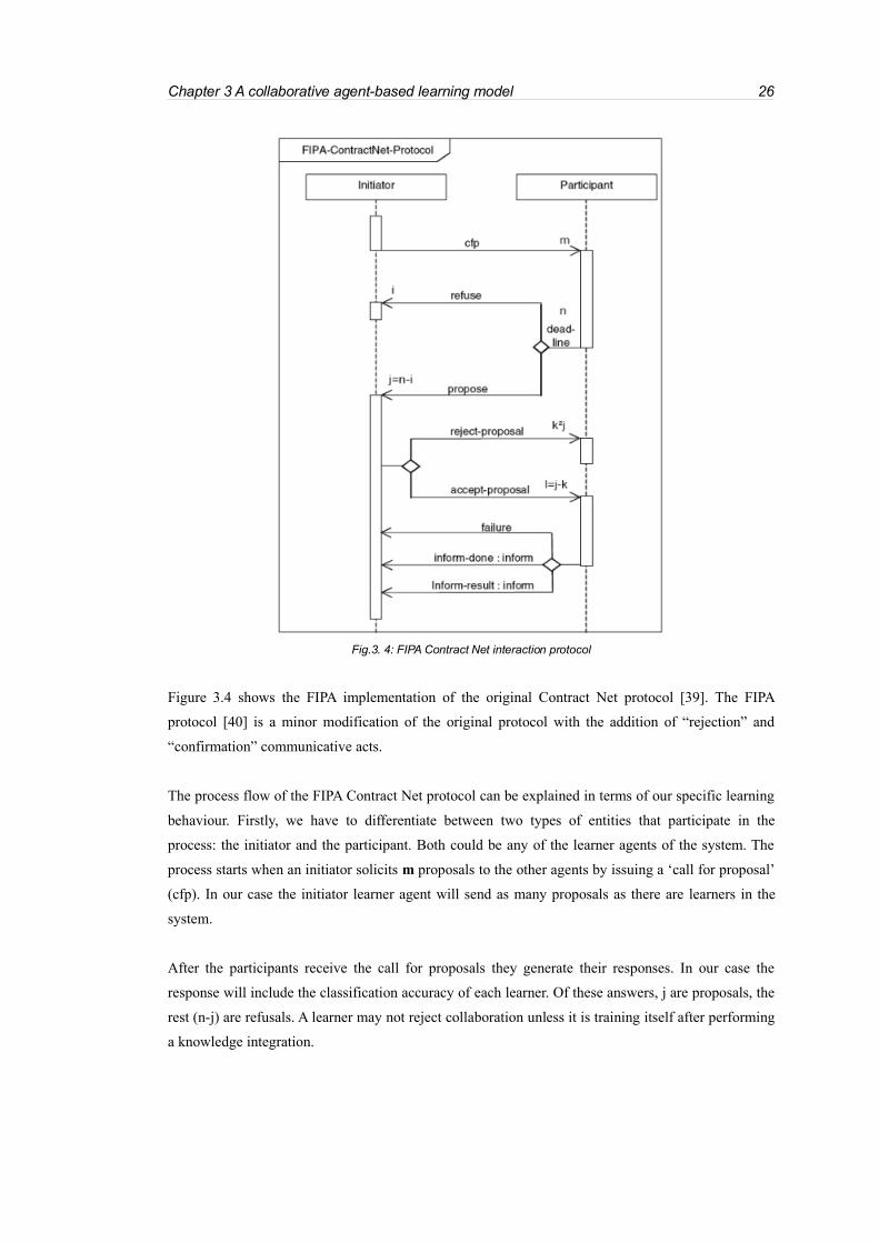
Chapter 3 A collaborative agent-based learning model 26
Figure 3.4 shows the FIPA implementation of the original Contract Net protocol [39]. The FIPA
protocol [40] is a minor modification of the original protocol with the addition of “rejection” and
“confirmation” communicative acts.
The process flow of the FIPA Contract Net protocol can be explained in terms of our specific learning
behaviour. Firstly, we have to differentiate between two types of entities that participate in the
process: the initiator and the participant. Both could be any of the learner agents of the system. The
process starts when an initiator solicits m proposals to the other agents by issuing a ‘call for proposal’
(cfp). In our case the initiator learner agent will send as many proposals as there are learners in the
system.
After the participants receive the call for proposals they generate their responses. In our case the
response will include the classification accuracy of each learner. Of these answers, j are proposals, the
rest (n-j) are refusals. A learner may not reject collaboration unless it is training itself after performing
a knowledge integration.
Fig.3. 4: FIPA Contract Net interaction protocol

Chapter 3 A collaborative agent-based learning model 27
Once the deadline elapses, the initiator evaluates the received j proposals and selects agents to
perform the task. In our case, one or no agents may be chosen by applying the aforementioned filters
and using one of the selection criteria outlined in section 3.4.2.
The agent owning selected proposal will be sent an ‘accept-proposal’ message and the remaining k
agents will receive a ‘reject proposal’ message. The proposals are binding for the participant, so that,
once the initiator accepts the proposal, the participant makes a commitment to perform the task.
Once the participant has completed the task, it sends a completion message to the initiator in the form
of an 'inform-done' or a more detailed message in an ‘inform-result’. However, if the participant fails
to complete the task a ‘failure’ message is sent.
3.5 Knowledge integration
The second step in the collaborative learning model consists of merging the knowledge of the two
learner agents. In particular, one of the learning knowledge integration functions is performed during
this stage using some of the learning knowledge of the agent selected in the previous stage. In this
section we propose different practical methods that are suitable for merging other agents’ knowledge
with our collaborative agent learning model.
Due to time limitations, not all operations from the collaborative agent framework could be analysed.
Hence, the integration learning knowledge problem had to be constrained. The integration learning
problem was defined by looking at two kinds of learning societies. The first is constituted of
homogeneous learners implemented using the same type of learning algorithms, and the second using
heterogeneous learning algorithms. In each type of society three different types of learning knowledge
to be integrated were considered: training data, classification outputs and hypotheses. For each of
these types of knowledge and for each type of society, we defined different integration operations.
Table 3.1 summarises the integration knowledge problem assumed and the integration operations
proposed for each situation.

Chapter 3 A collaborative agent-based learning model 28
Homogeneous Heterogeneous
Data Join Training Sets
Outputs
Merge Predicted classes
Merge Probability distributions
Merge Distances
to centroids
N/A
Hypothesis Merge Trees
Table3. 1: Matrix of integration knowledge operations
In the following section we will describe all the operations proposed in the matrix for collaborative
agent learning above.
3.5.1 Data merging
This operator aims to improve the prediction quality of local learners by incorporating training data
from other learners into local training sets. This can be described as an incremental data acquisition
method where each classifier (hi) is built using its particular learning technique (L) repeatedly, after
new data (Di) is gathered together. As a result, a new version of the classifier it is obtained (hi+1) from
this step. The following figure illustrates this method:
The details of this method are as follows:
1. The learner i request a percentage of random training samples of the provider learner j. The
percentage has to be limited by the system designer. The higher the value the more
communication is required.
2. The data is sent from learner j to learner i.
3. The learner i incorporates the samples received into its training set.
4. The learner i filters out duplicate data from its dataset.
Fig3. 5: Schema for data merging process

Chapter 3 A collaborative agent-based learning model 29
3.5.1.1 Applying the data merging operation in the collaborative learning model
This method, outlined in figure 3.6, is reasonably straightforward to deploy by following the
previously specified details for our collaborative learning model. Once the neighbour selection is
concluded and a learner (j) is selected for the knowledge integration stage, the initiator learner (i), who
starts the communication, sends a request for data to be transferred to the selected learner(j). When the
selected learner receives this request, it retrieves the data and sends it to the initiator learner. Upon
receipt of the data, the learner filters out repeated instances and rebuilds the classifier using the same
learning algorithm.
In the following diagram, this knowledge integration operation is described in terms of the
collaborative agent learning model :
This method is more appropriate for highly dynamic environments (e.g. distributed data sensor
networks) when new local data is frequently obtained or new data sites are added into the system. In
this kind of system this method allows the local sites to learn constantly from the other data sites
without overloading the network which might occur in centralised strategies where data is held in one
location.
However, the data merging operation exhibits some weakness in terms of computational efficiency
and data transfer security:
– It is costly as it requires to retraining the classifier once a new dataset is received.
Fig.3. 6: Data merging integration operation

Chapter 3 A collaborative agent-based learning model 30
– Large amounts of data are transferred across the network
– It is necessary to implement security protocols for transferring the data, such as data
anonymisation.
As an extension for data merging operations, improved results could be obtained by using a more
intelligent selection of data to transfer e.g. the most representative (relevant) in terms of the training
set, or to use other more complex data transfer methods from the literature, such as argumentation or
case-based reasoning [53].
3.5.2 Merging outputs
This type of integration operation relies on the traditional idea of combining classifiers predictions as
in distributed machine learning. We present different methods which use classification outputs from
multiple classifiers for deriving a joint prediction. Three types of classification outputs have been
identified for specific learning algorithms used in our system: predicted class labels, posterior
probabilities and distances to centroids:
– The predicted class is the resulting class after the classification of a sample.
– The posterior probabilities are the class membership probabilities for a given test instance. These
are calculated differently depending on the classifier method used.
– The distance to centroids method requires computing the distance between the instance to classify
and the mean of each of the possible classes that would be predicted by the centroids calculated
by the learning algorithm.
It is possible to obtain the predicted classes and probabilities from any learning algorithm. However
the distance to centroids output is specific to a type of learning algorithms based on functions such as
linear discriminants [41]. Therefore, we use only classifier merging operations for heterogeneous
types of classifiers for predicted classes and probability distributions, and homogeneous classifier
merging operations for classifiers with distance to centroids output.
The different merging methods for each of the classification output types defined is presented next.
3.5.2.1 Merging predicted classes
The first operation suggested for this kind of merging is the simple voting scheme [11, 29], which is
one of the most well known and most widely used methods. This method uses the classes predicted by

Chapter 3 A collaborative agent-based learning model 31
the classifiers. Each predicted class of a classifier represents a single vote. All votes from different
classifiers are counted and grouped by the type of class. Finally, the class which obtained the highest
number of votes will be the resulting predicted class.
Let Z will be the number of classifiers. Each classifier can output any of the following classes
{ω0,ω1,...ωn}, labelled with a c-dimensional binary vector [di,1, ..., di,c] Є {0,1}c, where c is the number
of classes. The binary vector will be formed applying the following rule:
1 if di labels ωj
d i,j = 0 otherwise
Then the plurality vote [29] method from n classifiers will result for class ωk if
∑i=1
Z
d i ,k=maxj=1
c
∑i=1
Z
d i , j
We will resolve ties arbitrarily (e.g. taking the first of the classes of the tie). This operation is often
called the majority vote and it is appropriate for situations exhibiting a great plurality of classifiers
since it smooths an individual classification function by looking at the consensus of the different
opinions based on the majority of the classifiers. The next figure shows the resulting separation
classifier boundary of 2 classes (-, +) after using the voting method over n different classifiers. It is
possible to observe the smoothing effect comparing the different decision boundaries as mentioned
above.
Other variations and alternatives related to this method exist in the literature. One of these is the
weight voting strategy [11,29] which covers the scenarios where the previous method is not effective.
For instance, if we had a number of poor classifiers, these would influence the final decision with the
same weight as the good classifiers, thereby possibly decreasing the accuracy of the merged classifier.
This method allocates a specific weight to classifiers determined by their classification performance.
The final prediction is computed by summing over all weighted votes and choosing the class with the
Fig.3.7: Resulting separation curves from simple voting method applied to n predictors

Chapter 3 A collaborative agent-based learning model 32
highest value. This alternative method could be a future improvement to the currently adopted
majority voting method.
3.5.2.2 Merging a posteriori class probability distributions
This technique is based on merging the estimates of the posterior class probabilities (supports) of the
different classifiers. This type of output can be defined as the degree of support a classifier has for a
particular class. In [11] two different methods are proposed for obtaining posterior probability
estimations. These depend on the type of classifier we are dealing with. One method is based on
discriminant scores for linear, quadratic, neural network or kernel classifiers, and another is based on
counts for trees classifiers. For simplicity, we outline the latter of these since tree classifiers are the
type of predictors used in our experimentation.
To estimate the posterior probability for an input instance x in tree classifiers, we calculate P(ωj| x),
j=1 ..., c, a quantity which represents the class proportion of the training data instances that reached a
leaf node (the maximum likelihood estimates). Let k1, ..., kc be the number of training instances
labelled as classes ω1,...ωc, respectively, at some leaf node t, and let K=k1+...+kc., the maximum
likelihood estimates for an instance x are:
P(ωj| x)=k j
K, j=1,. .. , c .
In this formula a problem can appear when the total number of instances for a leaf, K, is small, as the
estimated supports are unreliable. Besides, generally the tree growing strategies tend to also produce
leaves with supports 1 or 0 which are too extreme values for useful estimation. To solve this problem,
the Laplace estimate or correction is usually applied. The idea is to adjust the estimates so that they
are less extreme. The previous formula rewritten using the Laplace estimate is:
P(ωj| x)=k j1
Kc.
Lets us assume that the classifiers output the associated posterior probability using the previous
mechanism. This gives us a technique which combines several classifiers using their posterior
probability estimates and which may achieve better classification accuracies than isolated classifiers.
These operations are described in [11,29] as class-conscious and non-trainable combiners. They are
class-conscious since they label an input instance in the class with the largest a posteriori probability
obtained after some arithmetical operation which combines all the supports of the classifiers. And they

Chapter 3 A collaborative agent-based learning model 33
are non-trainable in that the classifiers resulting from the combination have no extra parameters that
need to be trained.
We have applied these techniques as a type of output integration operation for the collaborative
learning model. In the following we describe the steps required to perform these operations :
1. Classify an instance x with each of the Z classifiers which belong to the group of classifiers
to be combined, and obtain the vector of posterior class probabilities for these classifiers. The
classification will output di,1(x),... di,j(x) where di,j is the posterior probability of the classifier
i for the class j.
2. Merge the posterior probability for each class of all the classifiers. This is done using the
operation :
μj(x) = F [ d1,j(x),... di,j(x), ... dZj(x) ]
where F is an arithmetical operation which will be applied over d1,j(x),... dL,j(x), which is the
posterior probabilities vector from the Z classifiers over the jth class. This process will be
executed for each of the classes until we obtain a merging probability for each of the classes
μ1(x) to μj(x).
We use the following common arithmetical operations described in [11,29] as function F for
merging the posterior probabilities :
● Arithmetic mean
μj(x) = 1L∑i=1
L
d i , j x
● Maximum / minimum / median . For example, the maximum operation is:
μj(x) = maxi
d i , j x
● Product
μj(x) = ∏i=1
L
d i , j x
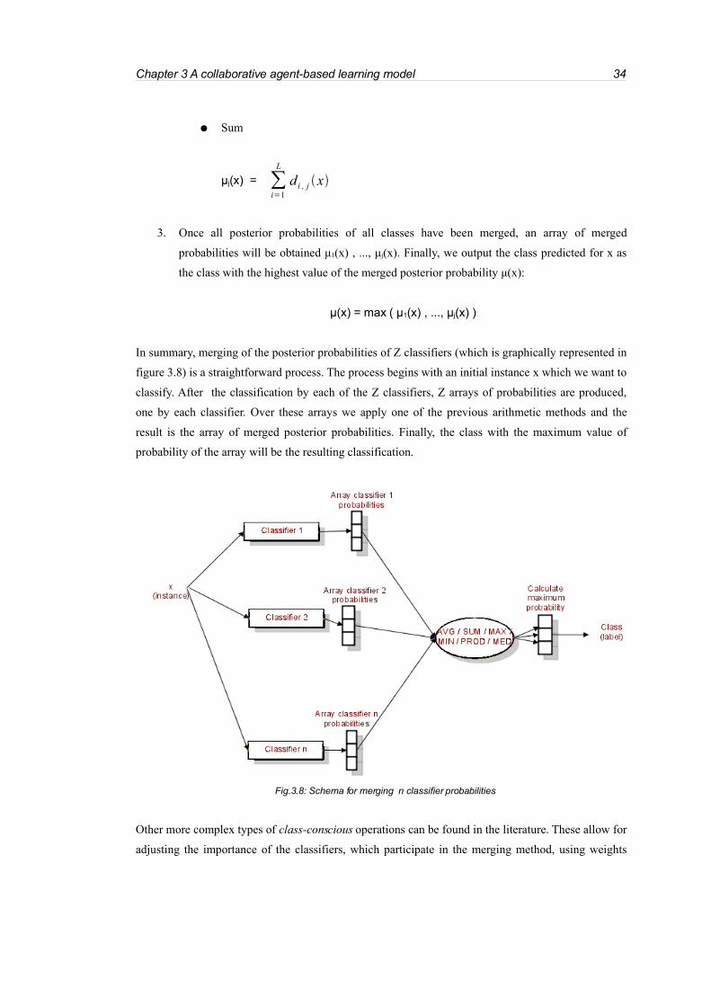
Chapter 3 A collaborative agent-based learning model 34
● Sum
μj(x) = ∑i=1
L
d i , j x
3. Once all posterior probabilities of all classes have been merged, an array of merged
probabilities will be obtained μ1(x) , ..., μj(x). Finally, we output the class predicted for x as
the class with the highest value of the merged posterior probability μ(x):
μ(x) = max ( μ1(x) , ..., μj(x) )
In summary, merging of the posterior probabilities of Z classifiers (which is graphically represented in
figure 3.8) is a straightforward process. The process begins with an initial instance x which we want to
classify. After the classification by each of the Z classifiers, Z arrays of probabilities are produced,
one by each classifier. Over these arrays we apply one of the previous arithmetic methods and the
result is the array of merged posterior probabilities. Finally, the class with the maximum value of
probability of the array will be the resulting classification.
Other more complex types of class-conscious operations can be found in the literature. These allow for
adjusting the importance of the classifiers, which participate in the merging method, using weights
Fig.3.8: Schema for merging n classifier probabilities
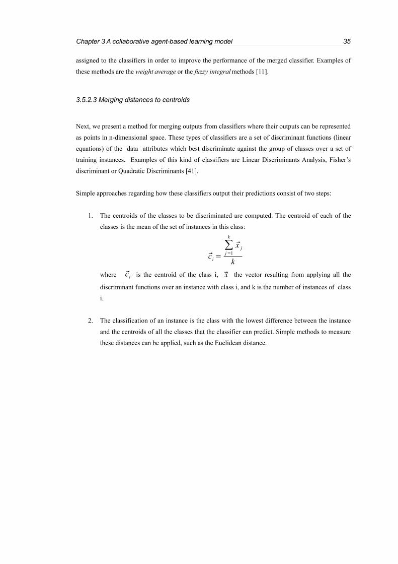
Chapter 3 A collaborative agent-based learning model 35
assigned to the classifiers in order to improve the performance of the merged classifier. Examples of
these methods are the weight average or the fuzzy integral methods [11].
3.5.2.3 Merging distances to centroids
Next, we present a method for merging outputs from classifiers where their outputs can be represented
as points in n-dimensional space. These types of classifiers are a set of discriminant functions (linear
equations) of the data attributes which best discriminate against the group of classes over a set of
training instances. Examples of this kind of classifiers are Linear Discriminants Analysis, Fisher’s
discriminant or Quadratic Discriminants [41].
Simple approaches regarding how these classifiers output their predictions consist of two steps:
1. The centroids of the classes to be discriminated are computed. The centroid of each of the
classes is the mean of the set of instances in this class:
c i =
∑j=1
k
x j
k
where c i is the centroid of the class i, x the vector resulting from applying all the
discriminant functions over an instance with class i, and k is the number of instances of class
i.
2. The classification of an instance is the class with the lowest difference between the instance
and the centroids of all the classes that the classifier can predict. Simple methods to measure
these distances can be applied, such as the Euclidean distance.

Chapter 3 A collaborative agent-based learning model 36
Figure 3.9 shows a representation of a dataset using a 2-class discriminant classifier. The two axes are
the two discriminant functions (D1,D2) of the classifier. The centroids of the two classes and the
boundary (straight line) which splits the instance space into two classes are plotted.
The merging method that we propose follows an idea similar to how a classifier outputs its
predictions. This simple merging operation consists of three steps:
1. Calculate an array of distances for each of the classifiers (e.g. using Euclidean distance)
between the class centroids and the instance to classify.
2. Calculate the average of all the classifier distance arrays.
3. Calculate the class predicted as the one with the lowest value of the array of averages.
Figure 3.10 summarises this process:
Centroid of class 1
Centroid of class 2
Fig.3.9: Dimension space of instances
Fig.3.10: Schema for merging n classifier distances to centroids

Chapter 3 A collaborative agent-based learning model 37
Alternative methods beyond using the average of vectors of distances can be devised, such as using
product, sum, maximum, minimum or median. More complex techniques that follow this approach
could be adjusting some weights over the classifier results in order to prefer some classifiers over
others.
3.5.2.4 Applying output merging in collaborative learning
In this section we describe the main design requirements for applying the output integration
operations in the collaborative learning model. However, these considerations are implementation
dependent and more domain-specific properties must be taken into account for a practical deployment.
These considerations are:
1. Each learner should implement some classification functionality where the classification
output taken from one of the three output types (class labels, probabilities or distances to
centroids).
2. The transfer of classifiers to use for integration. As a possible solution, we suggest the
transfer of classifiers from the selected to the integrator learner (fig.11) and perform the
integration operation in the integrator learner. This type of solution introduces an additional
requirement that the classifiers should be serialisables in order to be able to transfer them
through the network.
Another design alternative for result integration would be agent mobility although it entails
inherent security concerns [54], e.g. unauthorised access, denial of service, masquerade.
Another alternative solution would be to maintain a list of learners which form part of the
integrator learner ensemble in each integrator learner . Every time a classification with the
integrator learner is required, the classification results of the learners in the ensemble would
be required to merge them. This alternative is more networking intensive than the previous
solutions since it entails the transfer of classification results every time an evaluation of the
ensembles is performed in which this learner is involved.
3. The learners should maintain a list of classifiers that can be used for integration.
4. The learners must implement the output integration operation.
5. Each time a classification is requested, the learner will classify the instance using its list of
available classifiers, then the outputs will be integrated using the corresponding integration
operation, and the result of this operation will be output as the predicted class.
Next picture (3.11) shows the proposed design for this process:

Chapter 3 A collaborative agent-based learning model 38
In the above picture, initially the learner integrator asks for the classifiers of the selected learner. Once
the learner receives the classifiers, it adds then to its own classifiers for later evaluation. Every time an
instance classification with the integrator learner would be required, it will classify the instance with
all classifiers of the ensemble and it will merge the obtained results with the internal result merging
operation which it will have implemented.
3.5.3 Hypothesis merging
This section proposes an operation to integrate learning hypotheses or models (we use both terms
interchangeably). As mentioned in the background chapter, this integration operation is designed in
the spirit of collaborative learning, where the single learners only have local knowledge about the
domain and learn from others (through collaboration) in order to improve their performance.
This operation differs from output merging operation, since the models are not viewed as black boxes
to be combined depending on the quality of some output combination operation. The present model
merging operation identifies the interesting parts of the selected learner's model and modifies the
integrator learner’s model producing a new, richer model than that available before collaboration.
Moreover, this type of merging operation may lead to a better interpretability of the results rather than
the output merging operation since the predictions are not obtained using arithmetical operations
applied to results, but come from a single, uniform, merged model that can be inspected by the human
user directly.
The main problem encountered when merging hypotheses is the great diversity of classifier
Fig.3.11: Output merging integration operation

Chapter 3 A collaborative agent-based learning model 39
representations (rules, trees, probability functions, lineal equations...). This is due to the extraordinary
heterogeneity of learning algorithms in the literature. Ideally, a process would be required that allows
for dealing with a variety of classifier representations. In our work, instead of developing a generic
conversion process, we propose the use of a unifying (though limited) representation: the tree
representation. The reasons for choosing this representation are:
– Good understandability and readability for humans.
– Simple to process in computational terms.
– Straightforward to convert into rules (rules as tree branches). This property is useful for
conversion of n classifier representations into a single data structure.
3.5.3.1 Merging trees collaboratively
A technique for integrating hypotheses in the collaborative learning model based on merging tree
classifiers (ColTree) is presented next. The method attempts to increase the classification performance
of a learner while retaining the most interesting elements of the classification ability of the other
learner. For this purpose, the following four scenarios concerning two different classifiers (CL1 and
CL2), each drawn with a sphere which represents the instances classified correctly by a classifier
within the same dataset are considered:
Looking at figure 3.12, in the first scenario CL1 solves a subset of instances solved by
CL2. In the second scenario both classifiers solve instances that the other does not. In
the third scenario, CL2 solves a subset of instances solved by CL1. In the final
scenario, the instances solved by CL1 and CL2 are disjoint.
If CL1 is the classifier we wish to improve, then the situations of interest are those where CL2 is
predicting correctly and CL1 is not. From the diagram, the only scenario where CL1 can not improve
from CL2 is the third one. In all other situations CL2 would be interesting for our classifier.
Keeping this idea in mind, the following algorithm outlines the tree merging technique:
Fig.3.12: Different scenarios based on different classification abilities

Chapter 3 A collaborative agent-based learning model 40
1. Send CL1 form LEARNER1 to LEARNER2
2. In LEARNER2 classify using training set of
CL2 and comparing results of CL1 and
CL2
3. Select branches from CL2 that are
correctly classified and but where CL1 fails
4. Add selected branches to CL1
5. Send CL1 to LEARNER1
Table 3.2: Merging hypothesis method
This technique increases the knowledge of CL1 with those branches (rules) from CL2 which CL1
does not consider or where CL1 fails. This is in accordance with the collaborative agent learning
philosophy. However, this technique raises a number of implicit issues that have to be dealt with:
Firstly, the possibility of activating two or more rules (tree branches) for the classification of an
instance (contradictions/redundancies in verdicts). The following resolution methods have been
considered to resolve this problem :
– The verdict will be the rule with the largest probability class distribution.
E.g. If we had a classifier which can discriminate between 2 prediction classes (A,B) and
which internally would be composed of three rules with outputs (r1=A, r2=A,r3=B) and
with the following posterior probabilities for each rule (0.3, 0.5, 0.7), this method would
output class B as the rule (r3) has the largest estimate posterior probability.
– The verdict will be the class of the rules with the largest sum of the probability class distribution.
E.g. For the same previous example, this method would output class A as the rules (r1,r2)
have the largest cumulative probability.
– The verdict will be the class of the rules more frequently predicted, settled via voting.
E.g. For the same previous example, this method will output class A as this is the most
frequently predicted class.
We decided to use the last option since voting is the most common technique in machine learning for
solving opinion conflicts. However, this option needs to resolve draw situations where the same
number of votes are received for different classes. Therefore, we have decided a simple play-off
strategy where the first class will be the winning one.

Chapter 3 A collaborative agent-based learning model 41
Moreover, it is necessary to deal with the duplicity or redundancy of rules inside the merged classifier
result. The following filtering rules have been proposed to deal with this problem:
– Delete repeated rules.
– Delete conditions absorbed by another conditions inside of a rule, keeping the more general one,
e.g. (a<1) is absorbed by (a<2)
Another question is how to apply the present tree merging technique taking the large heterogeneity in
classifier tree representations into account. This is an implementation issue since in the literature we
can find numerous tree techniques implemented, but all of them have their own implemented data
structure (such as SimpleCart, BFTree, C4.5 and so on). The proposed solution consists of designing a
new common data tree structure (ColTree) which includes the functionalities to convert each of the
different tree structures into the new one.
The functionalities which constitute the tree-based hypothesis merging technique are summarised in
the following table 3.3.
1. Convert a particular tree classifier into a
common tree structure
2. Merge tree structures
3. Classify using merged tree structure
4. Remove conflict branches from the
common tree structure
Table 3.3: Main functionalities of tree merging technique
This functionalities of the common tree structure have been implemented in a new structure termed
ColTree. ColTree offers not only a framework for converting different heterogeneous tree classifiers
into the same format but also allows for merging them and performing classifications with the merged
result. Further implementation issues regarding ColTree and its functionality are described in chapter
4.
3.5.3.2 Incorporating tree merging in collaborative learning
When considering the integration of this method in the collaborative agent leaning model, we should
take the issues mentioned in the output merging operations (section 3.5.2.4) into account, with the
following additional considerations:
– Initially each learner will have translated its classifier into the ColTree structure. Once complete,
Chapter 3 A collaborative agent-based learning model 42
the learning integration process can proceed by following the algorithm explained in (fig.14).
– The models are modified by the receiver learner. The integrator transfers its model to the selected
other learner. There, the model is modified, and finally it is returned to the integrator. This process
has already been outlined in the output integration section (fig.3.11).
3.6 Performance evaluation
After the learning knowledge integration step, it is necessary to evaluate the performance of the
resulting classifier. For this, we propose to use a method based on holdout validation [26]. This
method consists of obtaining an independent set of instances just for testing purposes. This test set
should not be used in the training process in order to avoid possible poor quality performance
measurements caused by overfittting the classifier to these instances during training.
The evaluation process of a learner will consist of:
1. Classifying each of the test set instances with the learner’s internal classification model.
2. Obtaining the quality measurement of the model using the function defined in section (3.4.2)
which is the percentage of the correctly classified cases with respect to all cases in the test
set. As was mentioned above, this performance function is a simple way of obtaining a
quality measurement and much more advanced methods could be used.
Regarding the test set to use, we suggest having the same test set for all learners. This ensures that the
comparisons of classification performances of the learners during the selection step of the
collaborative learning will be consistent. It also implicitly requires the learners to have common
access to the same test set.
In some situations where this condition is not realistic we would allow the learners to have their own
local test set. However we believe that the different local test sets at least should exhibit a certain
similarity in order to make the selection criteria coherent.
3.7 Knowledge update
Finally, once the classification quality of the integrated classifier has been calculated, the learner
should make a decision regarding learning knowledge update. This decision concerns updating the
learning knowledge using new information from the previous interaction if the accuracy of the
integrated is higher than the previous accuracy of the learner. i.e.

Chapter 3 A collaborative agent-based learning model 43
update if g i1g i .
This simple decision criterion is based on the classification accuracy measure (section 3.4.2).
However more complex updating operations could be considered using other measurements such as
ROC curves [42] or F-measures [43].
The learning knowledge to be updated with the integrated one will be the new classifier, the current
quality of the model, the current version of the learner and the list of the previous learner agents
interacted with.
It is important to independently mention that if the updating criterion is satisfied the learner should
update the list of previous interactions with the identifier of the learner interacted with in order to
avoid repetition of the same interactions. This makes the system more efficient in time complexity and
ensures less communication overload.
3.8 Termination criterion
After the update process the learner continues its collaborative learning to improve its classification
capability. This learning process continues indefinitely. However, a termination criterion for the
collaborative learning process could avoid unnecessary communication in systems where new nodes
are not expected in the network frequently. E.g. The learners each time they start a new learning step
they need to broadcast to all the agents in order to obtain the learners available.
We propose such a criterion consisting of stopping the learner (putting it in a waiting state) when the
learner, L1, has interacted with all other learners in the system taking into account that once L1 has
interacted with another learner and updates itself (satisfactory interaction) then L1 has to consider all
learners in the system again except those have been interacted before successfully. Therefore we
require to obtain the maximum number of learner interactions to know when to stop the learners.
We obtain the estimation of the maximum number of interaction for a particular learner (maxInt) as,
over n-1 times, the sum of all available learners, so that each time one learner less will be available as
it will be the one the learning agent interacted with. I.e. :
maxInt=∑i=1
n−1
i ,
where n would be the number of learners in the system. This value is a worst-case estimate because
the learner always updates its knowledge with the last possible learner found. Therefore this value is

Chapter 3 A collaborative agent-based learning model 44
too pessimistic as a termination criterion and could be too extreme, for example a learner who does
not perform a successful interaction with any of the other learners in the system or a learner who
would perform successful interactions with all other learners at the very first opportunity. In these
cases the number of interactions would be n-1 (the number of all learners except the integrator) which
is a much lower value than that specified by the previous formula.
Therefore we propose the following criterion in order to avoid an excessive number of interactions:
Number of interactions= maxInt∗ p/100 ,
where p would be a parameter defined a priori by the designer and which would represent the
percentage of interactions allowed to perform. In order to apply this criterion the learner must keep
track of the number of interactions performed so far.
Finally, if new learners appear in the system, the learners that have stopped interacting should be
notified and be activated again in order to attempt collaborations with the new agents.
3.9 Conclusions
In this chapter we have presented an agent-based collaborative learning model. This model is inspired
by the multiagent learning view proposed in the MALEF framework [1], whose motivation has been
described at the beginning of the chapter. The MALEF collaborative learning focuses on the real use
of autonomous and independent learners which engage in collaboration among each other in order to
increase their classification accuracy. Our model is inspired by these ideas and advances this
framework by proposing a more practical instantiation of collaborative learning for distributed data
mining domains where data sharing is limited. This alleviates some weaknesses of the abstract
framework, as reflected in the redefinition of the collaborative learning step. In particular, four well-
defined stages have been identified as part of each learning step. Each of these stages has been
explained in detail and several methods and criteria have been introduced for each of them so as to
make the implementation of this model feasible in practice.
In the next chapter we will focus on the implementation of the methods that constitute the
collaborative learning model.

Chapter 4 Implementation 45
Chapter 4
Implementation
4.1 Introduction
In this chapter we focus on the implementation produced in order to evaluate the collaborative
learning model and its different configurations as presented in the previous chapter.
A variety of different factors can affect the performance of our collaborative learning model, some of
which depend on the environment in which it is deployed, like the number of learners in the system,
the learning algorithms used, or the size of the datasets used for training the learners. Other factors
depend on the internal configuration of collaborative learning itself, such as the neighbour selection
criterion chosen, the knowledge integration method employed, and so on.
To account for these factors, we developed an application that permits the testing of the collaborative
learning model using different parametrisations of the environment or of the learning components
themselves. In the following sections, we provide the details of the design and implementation of this
application.
4.2 Objectives of the implementation
The motivation of developing a test application is to investigate how effective collaborative learning is
and how it performs in its overall tasks. These aims are too general to be applied directly to the
specification of the application, and we therefore have to refine the requirements and identify what
exactly the application should evaluate.
Regarding the environment in which the collaborative learning model is deployed, we determined the
following system parameters to be most significant :
– Classifier heterogeneity in the environment.
– Number of agents in the system.

Chapter 4 Implementation 46
– Size of training datasets.
Further aspects to analyse regarding the different methods proposed for the collaborative learning
model include:
– The use of a greedy accuracy selection tactic versus a randomised accuracy weighted strategy.
– The use of methods for environments in which transfer of small amounts of data is allowed.
– The use of methods for environments in which classification outputs may be communicated.
– The use of methods for environments in which local models may be communicated.
– The effect of allowing more interactions between the learning agents.
The last of these variables provided the performance measure for our learning strategy regarding other
learning strategies. We considered two extreme strategies as benchmarks: the centralised strategy and
the distributed isolated strategy. The centralised strategy consists of creating a single learner that
contains a classifier trained on all the training data available in the system. Distributed isolated
learning consists of different learners where each has a classifier trained on a local partial dataset and
there is no communication among the learners.
These benchmark learning strategies led to the design of an application that allowed the specification
of different environment configurations (scenarios) and different learning experiments to run in which
we wanted to evaluate how well interacting learners perform as opposed to non-interacting ones
(“isolated” case) and omniscient ones (“centralised” case). In the next sections, we describe the design
and the implementation of the experimental application.
4.3. Application architecture overview
Our main objective was to develop an experimental, highly configurable application with which to
implement the collaborative learning method, which would easily enable us to obtain results from the
execution of a variety of different experiments. Since any distributed environment implementation
involves the additional implementation of communication and control mechanisms, which are costly
to implement, we designed a sequential application that emulates distributed learning environments in
a deterministic way in order to concentrate our efforts on the evaluation of the collaborative learning
model and their methods. The sequential application algorithmically is not different from a distributed
solution since all methods and criteria which constitute the collaborative model (Chapter 3) have the
same results regardless of whether the application is distributed. Thus, we have left the
implementation in a real agent-based software environment to future work.
Three different types of learning experiments can be executed: centralised, distributed isolated and
distributed collaborative learning. These types emulate two kinds of architecture designs: a centralised

Chapter 4 Implementation 47
environment that is straightforward to design in a single local machine as by definition it operates
locally; and the distributed learning configuration that operates on a single data source in the network
which represents a partition of the whole dataset. In this way, we can emulate distributed data nodes as
partitions of a given dataset.
Classifier heterogeneity in a distributed learning environment has been emulated by assigning a
different learning algorithm to each partition. Finally, the multiagent environment of the collaborative
learning strategy has been emulated by using the classifiers as agent learners, implementing agent
behaviour as a sequence of methods to be performed by the classifier, and agent communication by
manipulation of the list of classifiers to interact with.
Example: an environment with 10 data sites and with 10 distributed classifiers will be
implemented locally by creating 10 partitions of the data for training, and, then, for each of
these partitions we will build the corresponding classifier.
Further details of the design and implementation are described in the following sections.
4.4 Functional design of the application
The application should permit the execution of several experiments over different environment
configurations in order to exhaustively test our learning model. For this reason, we have designed an
application where we first specify the environment parameters and the learning experiments to be run
in these environments, then the application executes these experiments, and finally summary results of
these runs are produced.
These functions are detailed in the application execution flow diagram (Fig.4.1).
Fig4. 1: Execution flow of the application

Chapter 4 Implementation 48
In the above diagram we observe that the first operation to be performed refers to the definition of the
scenarios in which the experiments are executed. This involves the initialisation of information such
as the size of the training and test datasets, the number of data partitions and the learning algorithms to
be used for building classifiers.
The second operation consists of three different processes. Initially, the setup of the learning
experiments is performed by choosing the learning strategy to execute, or in the case of collaborative
learning, the integration method, the selection criteria and the termination criteria among other
configuration parameters. After this, the learning experiment is executed. Finally, the learning
experiment results are stored.
The last operation stores the output of the results of all the experiments executed. The idea is to
provide different plots, ratios and matrices of results in order to make further analysis and evaluation
possible.
All these functionalities and their details are described in the following sections, however the specific
values of the configurations and the learning results obtained are presented in the evaluation chapter.
4.4.1 Setup of the learning environment
This process defines the learning environment in which the experiments are run. We have identified
the following parameters by which to identify a scenario:
– The dataset. This is the data for the learning process.
– The number of agents or partitions of the dataset. There is a correlation between the number of
partitions and agents because in our system each agent is assigned to a different partition.
– The size (number of instances) of a partition of the training dataset
– The size of the test sets if it is a partition of the training set.
– The list of algorithms to be used for building the classifiers of the system. A single method in this
list would imply a homogeneous environment. On the contrary, a heterogeneous environment will
have the choice of more than one classifier algorithm to use.
4.4.2 Running the learning experiments
This functionality concerns the execution of the learning experiments, and involves three operations:
parametrisation of the experiments, running the experiments and storage of the results.

Chapter 4 Implementation 49
4.4.2.1 Parametrisation of the learning experiments
The following parameters are required in order to run an experiment:
– The type of the learning strategy to use. As we have commented previously, apart from
collaborative learning two other learning strategies have been provided in order to compare its
performance compared to the centralised and the distributed isolated learning strategies.
– Other parameters have to be specified that only affect the collaborative strategy:
– The neighbour selection strategy to use.
– The collaborative integration method which indicates the knowledge integration method
to apply.
– The termination criterion which determines when to terminate the collaborative learning.
4.4.2.2 Design of the learning strategies
In the next sections we focus on the design details of each of the implemented different learning
strategies. These designs assume a previous process which divides the whole dataset into a training
and an independent test set following the parameters mentioned in section 4.3.1.
4.4.2.3 The centralized learning strategy
Centralised learning (Fig.4.2) relies on the use of all the training data for building a central classifier.
In scenarios which have one learning algorithm for building classifiers, a single classifier is built and
evaluated (section 3.4.2) using the test set. However, in the case of scenarios with a choice of different
learning algorithms, the centralised strategy is implemented building as many classifiers (using all the
training set) as learning algorithms are available. After this, all the classifiers are evaluated using the
test set. The performance resulting from each experiment is the average and standard deviation of the
accuracy obtained by all classifiers. We propose this measure for obtaining the estimated performance
of the defined strategies, since it defines a global measure of the method performance applicable to all
classifiers. We preferred a global measure rather than focusing on maximum or minimum performance
values since those results could be influenced by the quality of the particular data partition or learning
algorithm of a classifier.
The next figure presents an example of a centralised learning process for an heterogeneous scenario,
with three different learning algorithms.

Chapter 4 Implementation 50
As can be observed from the above figure, three different classifiers are learned using each of the
learning algorithms but with the same training data.
4.4.2.4 The distributed isolated learning strategy
The distributed learning strategy bases its design on building as many classifiers as partitions from the
training data as required. The number of partitions and their sizes are specified a priori.
In the homogeneous scenario, the same learning algorithm is used to build all classifiers. As explained
in the previous strategy, the evaluation of this scenario is done using the averages of all the accuracies
obtained from all the classifiers.
In the heterogeneous scenario (Fig.4.3), we have different learning algorithms for building the
classifiers from the data partitions. Constructing these classifiers will be done using one of the
learning algorithms on each data partition. This assignment must be done to ensure the learning
algorithm is used a equal number of times. As in the homogeneous case, the evaluation criterion for
this learning scenario will be the average of the accuracy of all classifiers.
Fig.4.2: Design of centralised learning for the heterogeneous scenario
Fig.4.3: Design of the distributed isolated learning in a heterogeneous environment
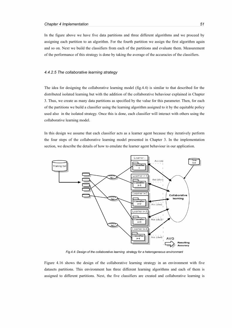
Chapter 4 Implementation 51
In the figure above we have five data partitions and three different algorithms and we proceed by
assigning each partition to an algorithm. For the fourth partition we assign the first algorithm again
and so on. Next we build the classifiers from each of the partitions and evaluate them. Measurement
of the performance of this strategy is done by taking the average of the accuracies of the classifiers.
4.4.2.5 The collaborative learning strategy
The idea for designing the collaborative learning model (fig.4.4) is similar to that described for the
distributed isolated learning but with the addition of the collaborative behaviour explained in Chapter
3. Thus, we create as many data partitions as specified by the value for this parameter. Then, for each
of the partitions we build a classifier using the learning algorithm assigned to it by the equitable policy
used also in the isolated strategy. Once this is done, each classifier will interact with others using the
collaborative learning model.
In this design we assume that each classifier acts as a learner agent because they iteratively perform
the four steps of the collaborative learning model presented in Chapter 3. In the implementation
section, we describe the details of how to emulate the learner agent behaviour in our application.
Figure 4.16 shows the design of the collaborative learning strategy in an environment with five
datasets partitions. This environment has three different learning algorithms and each of them is
assigned to different partitions. Next, the five classifiers are created and collaborative learning is
Fig.4.4: Design of the collaborative learning strategy for a heterogeneous environment

Chapter 4 Implementation 52
performed for each of these classifiers. Measurement of the quality of this strategy is done based on
the average accuracy resulting from the accuracy of the classifiers after collaboration between them as
explained in the initial strategy.
4.4.3 Preparation of the learning results
In order to analyse the performance of the learning experiments, we will store the execution time and
the accuracy achieved. For the collaborative learning strategy, we will store this information every
time a collaborative interaction is performed. In this way we will be able to conduct a more accurate
analysis of the learning process.
As we will deal with a large number of scenarios and a lot of experiments, it is difficult to manage and
analyse the learning processes. We have developed simple ratios to aid in discerning information from
the data. These ratios are :
– The classification accuracy average and the standard deviation across the accuracies of all
classifiers in each interaction.
– The average time and the standard deviation of all classifier accuracies for each interaction.
Moreover, from the experiment result matrix, we have computed the following graphs:
– Accuracy per interaction
– Time per interaction
– Accuracy of the methods with an increasing number of agents
– Accuracy of the methods with increasing sizes of training datasets.
4.5 Implementation of the application
The application has been implemented using Java technology because, among other advantages, it
offers object oriented technology; it is broadly used and lots of pre-existing libraries are available;
and, it offers an easy environment for programming. Also, we have used the Weka [33] open source
library for machine learning tasks, such as classifier building, training and evaluation. We have chosen
Weka because it offers three principal advantages over most other data mining software packages.
Firstly, it is open source, which not only means that it can be obtained for free, but it is maintainable,
and modifiable. Secondly, it provides a number of state-of-the-art machine learning algorithms that
can be deployed in any given problem. Thirdly, it is implemented in Java and hence fully compatible
with the implementation of our application.

Chapter 4 Implementation 53
Finally, for data testing we have used datasets from the UCI [32] machine learning repository, which
is one of the largest free on-line repositories available.
4.5.1 Class diagram
The structure of the application is summarised in the following schema (Fig.4.5). The schema does
not show the classes, attributes or operators that are less important for easy of readability.
The principal classes of the application are MakeFullTest and MakeOnceTest. The main() method of
the MakeFullTest class is the starting point to run the application. In this method, the parameters of
the environment are loaded. After this, for each of the defined environments a MakeOnceTest object
Fig.4.5: Application class diagram

Chapter 4 Implementation 54
is created and the main() method is called to run the learning experiments.
In the next sections we explain the implementations of the three types of learning experiments
(centralised, distributed isolated and distributed collaborative) that are performed within the main()
method of the MakeOnceTest class.
4.5.2 Implementation of the centralised learning strategy
The design of this strategy (section 4.3.2.3) and its implementation within the test application is
described by the following pseudo-code.
Initially the data is divided into training and testing datasets. This process is done in the
CreatePartitionData() method, which has the dataset, the size of the test data and the number of data
partitions as input values. For the centralised strategy, no partitioning of the training data is performed.
After this, a loop is used for each of the learning algorithms defined for this experiment. Inside this
loop, a classifier is built using the buildLearnerAg() operation, which has as input parameters the data
partition and a learning algorithm. Next, the evaluation of the classifier is done using the
evaluateModel () method from the Weka class Evaluation. This operation returns the accuracy of the
current classifier. Finally, the accuracy and time results are stored in the resultMatrix array.
4.5.3 Implementation of the distributed isolated learning strategy
The design of this strategy (section 4.3.2.4) and its implementation within the test application is
described by the following pseudo-code.
Fig.4. 6: Pseudo-code for centralised strategy
1: CreatePartitionData (DataSet,partitionData,testData,sizeTest,numPartitions)
2: for all algType in listClassifierAlgorithms
3: {
4: initTime (time)
5: CL=buildLearnerAg (partitionData,algType)
6: acc=evaluateModel (CL, testData)
7: storeResults (resultMatrix,acc,time)
8: }

Chapter 4 Implementation 55
As in the centralised algorithm the whole dataset is divided into training and testing datasets. This
process is done in the CreatePartitionData() method which also creates as many partitions of the
training data as specified in numPartitions. The partitions are output in the partitionData array.
A loop for each of the partitions is performed in which we obtain the learning algorithm for building
the classifier using the selectClassifierAlgorithm() method. This method implements a simple
operation (described in section 4.3.2.4) in order to ensure that the algorithms are used equally often.
Then the classifier is built using the buildLearnerAg() operation. Next, the evaluation of the classifier
is performed to obtain the accuracy of the current classifier. Finally, the accuracy and time results are
stored in the resultMatrix array.
4.5.4 Implementation of the collaborative learning strategy
Several implementation decisions have been made in order to make the collaborative learning method
feasible using an object oriented approach:
– The role of the learner agents is assigned to the classifier objects, and the agent communication
abilities (sending and receiving messages) are implemented by providing each classifier with the
list of all classifiers in the system to interact with.
– Each classifier in the agent collaborative learning model iterates over the list of classifiers in the
system. Inside each loop this classifier sequentially calls the methods which constitute a
collaborative learning step as described in the Chapter 3.
In the next section we describe the details of the algorithm that implements the collaborative learning
strategy.
Fig.4. 7: Pseudo-code for distributed isolated strategy
1: CreatePartitionData (DataSet,partitionData[], testData,sizeTest,numPartitions)
2: for all p in numPartitions
3: {
4: initTime (time)
5: algType=selectClassifierAlgorithm()
6: CL=buildLearnerAg (partitionData[p], algType)
7: res=evaluateModel (CL, testData)
8: storeResults (resultMatrix,res, time)
9: }

Chapter 4 Implementation 56
4.5.4.1 Collaborative learning algorithm
The design of this strategy (section 4.3.2.5) was implemented within the test application by using the
pseudo-code shown in figure 8. The algorithm assumes an initial division of the dataset into training
and test set. Also a partitioning of the training set and the building of their classifiers using single
elements of this partition is assumed. The classifiers are stored in the list of classifiers
“listClassifiers”.
Fig.4. 8: Pseudo algorithm collaborative learning strategy
1: sortingClassifiers(listClassifiers)
2: For all cl1 in listClassifiers
{
3 interactions=1
4: satisfiedInteraction=false
5: classifiersVisited.Add(cl1)
6: while(classifiersVisited.num()<listClassifiers.num()) && (! stopCriteria(in teractions))
{
7: j=0
8: if (searchPolicy==”Greedy”) cl2=listClassifiers.get(j)
9: else cl2=weightRandomizedNext(visited, listClassifiers)
10: satisfiedInteraction=false11: While ( (cl2!=null) && (! stopCriteria(interactions)) && (!satisfiedInteraction))12: {13: if(! classifiersVisited.contains(cl2))14: {15: auxcl1=mergeClassifiers(cl1,cl2)
16: evaluateClassifier(auxcl1)17: if updateClassifier(cl1,auxcl1)
{18: cl1=auxcl119: satisfiedInteraction=true
20: classifiersVisited.add(cl2)21: }22: storeResults()23: Interactions++
24: }25: j++
26: if (searchPolicy==”Greedy”) cl2=listClassifiers.get(j)
27: else cl2=weightRandomizedNext(visited, listClassifiers)
28: }
29:30: }31: classifiersVisited.clear()
32: }

Chapter 4 Implementation 57
The algorithm is a loop over all classifiers in the system where for each of the classifiers (cl1) the
collaborative learning process is performed. This process ends when one of the three following
conditions are fulfilled:
– The termination criterion is satisfied, which implies (section 3.8) that the number of classifier
(cl1) interactions done is equal to the maximum number of interactions as specified.
– The current classifier (cl1) has satisfactorily interacted with all the classifiers in the system. A
successful interaction with a classifier (cl2) implies that cl2 is used to update cl1. In this case cl2
is included in the classifiersVisited array.
– No successful interaction was possible with any of the classifiers in the system.
If the termination condition is not satisfied a new collaborative learning step is created with the
classifier cl1. A collaborative step is also an iterative search among the classifiers (cl2) which may
provide a successful interaction for cl1. This search begins by assigning a classifier cl2, which had not
been interacted with, through the selection criterion (lines 8,9). Once cl2 is obtained the knowledge
merging operation (line 15) is applied obtaining an auxiliary classifier (auxcl1). Then, an evaluation of
the auxcl1 is performed (line16), and if it satisfies the update condition using the updateClassifier()
method, then cl1 is updated with auxcl1 (or its training data, depending on the knowledge integration
operation employed) and we take note that a new classifier has been successfully interacted with.
In the next sections we will focus on the implementation of the neighbour selection, knowledge
integration and evaluation operations in order to clarify how these processes are implemented in more
detail.
4.5.4.2 Neighbour selection implementation
The greedy and randomised neighbour selection criteria defined in section 3.4 have been implemented
for this purpose.
– The greedy criterion is implemented as a loop over a sorted classifier list. This list is sorted by
classification accuracy. We have implemented simple sorting method sortingClassifiers() in the
makeOnceTest class which performs this operation. The first classifier to interact with will
therefore be the first one in the sorted list.
– The randomised criterion is implemented using the weightRandomisedNext() method of the
makeOnceTest class. This method returns the next classifier to interact with among the list of
available classifiers. The randomised criterion makes the collaborative learning non deterministic,

Chapter 4 Implementation 58
which will lead to different results in each simulation. For this reason, the evaluation of this type
of configuration will be obtained from the average of different executions. We show the code
implemented for the randomised accuracy algorithm:
This method has been described in detail in section 3.4.2. In brief, the algorithm obtains the list of
classifiers which have not been used successfully (restClassifiers). This list is assumed to be sorted by
classifier accuracy. Then, a search of the first classifier (cl) is performed over this sorted list where its
relative accuracy, the sum of the accuracy of the available classifiers plus the previous classifier
accuracies, is greater than a certain random value (r). If all classifiers have been visited the method
does not return any classifier.
4.5.4.3 Implementation of the integration operations
Once the learner is selected knowledge integration is performed. We have implemented the three kinds
of integration methods proposed in Chapter 3:
1. Data merging
This method is an implementation of the merging data operation described in section (3.5.1). This
method (fig.4.10) is implemented by the datajoininglearning method of the makeOnceTest class.
Fig.4. 9: WeightRandomizedNext method for the weighted randomised neighbour criterion
1: Classifier weightRandomNext(listClassifiers , classifiersVisited)2: {3: double sum=0.0;4: double prob=0.0;5: double r= random(0,1);6: boolean found=false;7: restClassifiers= classifiersNotVisited (listClassifiers , classifiersVisited);8: for (cl : restClassifiers )9: sum=sum+(cl.accuracy() / 100.0);10:11: while(! Found) && (restClassifiers.hasNext())12: {13: cl=restClassifiers.next();14: prob=prob+((cl.accuracy/100.0)/sum);15: if (r<prob) found=true;16: else cl=restClassifiers.next();
17: }18: if (found) return cl;19: else return null;20: }
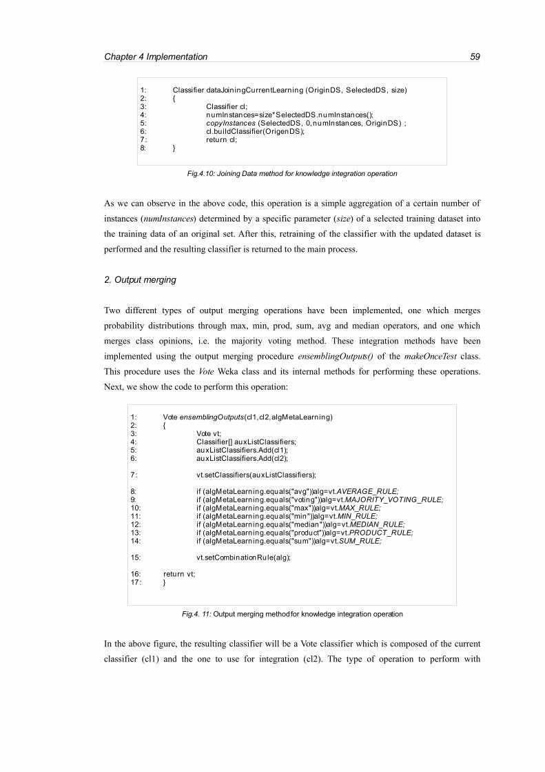
Chapter 4 Implementation 59
As we can observe in the above code, this operation is a simple aggregation of a certain number of
instances (numInstances) determined by a specific parameter (size) of a selected training dataset into
the training data of an original set. After this, retraining of the classifier with the updated dataset is
performed and the resulting classifier is returned to the main process.
2. Output merging
Two different types of output merging operations have been implemented, one which merges
probability distributions through max, min, prod, sum, avg and median operators, and one which
merges class opinions, i.e. the majority voting method. These integration methods have been
implemented using the output merging procedure ensemblingOutputs() of the makeOnceTest class.
This procedure uses the Vote Weka class and its internal methods for performing these operations.
Next, we show the code to perform this operation:
In the above figure, the resulting classifier will be a Vote classifier which is composed of the current
classifier (cl1) and the one to use for integration (cl2). The type of operation to perform with
Fig.4. 11: Output merging method for knowledge integration operation
1: Vote ensemblingOutputs(cl1,cl2,algMetaLearning)2: {3: Vote vt;4: Classifier[] auxListClassifiers;5: auxListClassifiers.Add(cl1);6: auxListClassifiers.Add(cl2);
7: vt.setClassifiers(auxListClassifiers);
8: if (algMetaLearning.equals("avg"))alg=vt.AVERAGE_RULE;9: if (algMetaLearning.equals("voting"))alg=vt.MAJORITY_VOTING_RULE;10: if (algMetaLearning.equals("max"))alg=vt.MAX_RULE;11: if (algMetaLearning.equals("min"))alg=vt.MIN_RULE;12: if (algMetaLearning.equals("median"))alg=vt.MEDIAN_RULE;13: if (algMetaLearning.equals("product"))alg=vt.PRODUCT_RULE;14: if (algMetaLearning.equals("sum"))alg=vt.SUM_RULE;
15: vt.setCombinationRule(alg);
16: return vt;17: }
Fig.4.10: Joining Data method for knowledge integration operation
1: Classifier dataJoin ingCurrentLearning (OriginDS, SelectedDS, size)2: {3: Classifier cl;4: numInstances=size*SelectedDS.numInstances();5: copyInstances (SelectedDS, 0,numInstances, OriginDS) ;6: cl.buildClassifier(OrigenDS);7: return cl;8: }

Chapter 4 Implementation 60
ensembles of classifiers is also specified in this method.
3. Tree model merging
To make this type of integration the classifiers must be previously converted into ColTree classifiers.
The ColTree classifier class was developed specifically to allow tree model integration between
heterogeneous classifiers as explained in section 3.5.3. As we commented there, the ColTree classifier
represents a common structure into which to convert any type of Tree classifier. Thus, ColTree is a
class which holds an array of heterogeneous tree branches. Each of these tree branches is represented
by a dynamic list of nodes, where each node is a ColBranchTree object that has a link to the successor
node which will be another ColBranchTree object.
3.1 ColTree conversion process
We have implemented a process to convert tree-based classifiers as defined in Weka into a ColTree
classifier. This is done by the buildColClassifier() method of the ColTree class where the Weka
classifier is passed as an input and a ColTree classifier is returned. Figure 12 shows the code
forColTree conversion:
In the above figure we show a particular piece of code for converting the SimpleCart Weka tree
classifier into a ColTree classifier. In order to achieve this conversion, we compute the array of all
branches of the tree classifier which will be obtained using the getAllTreeBranchesCBT() method.
Once this is done, the branches are added into the ColTree classifier and then node redundancies in the
branches are deleted using a compacting process in the compactRules() method. This two processes
are detailed in the next paragraphs
3.2 Obtaining Tree branches
The ColTree conversion operation consists of performing a loop over all nodes of the Weka tree in
order to extract the list of branches. This mechanism requires access to the internal attributes of the
tree classifier, therefore we have had to implement the conversion procedure within the Weka Tree
classifier framework. In order to demonstrate the feasibility of this conversion we have implemented
Fig.4. 12: ColTree conversion of a base Weka classifier (SimpleCart)
1: ColTree buildClassifier(SimpleCart m_Classifier1) {
2: addBranches(m_Classifier1.getAllTreeBranchesCBT());3: compactRules();4: return (this);
5: }

Chapter 4 Implementation 61
this routine for three different Weka Tree classifiers: SimpleCart, BFTree and REPTree (section 2.3.2).
Below we show the particular implementation (fig.4.13) of the method for converting the SimpleCart
classifier into an array of ColBranchTree branches. This is done in the getAllTreeBranches() method
which consists of a loop over all the leaves of the tree. For each leaf, the getTreeBranchCBT() method
is executed to obtain the branch with this leaf.
The above method calls the getTreeBranchCBT() method (Fig.4.13) in order to return the branch of the
tree with the input leaf. In particular, this method returns a new colBranchTree object which is the
initial node of the list which represents a branch of the tree.
In the above method (fig.4.14) a recursive search is done through the nodes of SimpleCart tree until
the input leaf node is reached. For each node of the tree, a new ColBranchTree object is created using
the convertToCBT() method where the internal values of the attributes from the SimpleCart node are
Fig.4.13: Method which returns a vector of ColBranches for a SimpleCart classifier
public Vector<colBranchTree> getAllTreeBranchesCBT(){
Vector<colBranchTree> vSC Vector<SimpleCart> leafListcolBranchTree sc;for (in t i=0;i<this.numLeaves();i++){
sc=getTreeBranchCBT(leafList);vSC.add(sc);
}return vSC;
}
Fig.4. 14: Method for converting a single branch of a SimpleCart tree to a ColBranchTree.
colBranchTree getTreeBranchCBT(Vector<SimpleCart> leafList) {
int j=0;boolean fi=false;int prev=0;colBranchTree sc=this.convertToCBT();if(m_isLeaf){
if(!leafList.contains(this)) leafList.add(th is);else sc= null;
}else{while ((j<2)&& (!fi)){
prev=leafList.size();sc.setM_Successors(m_Successors[j].getTreeBranchCBT(leafList));if (prev<leafList.size()) {
fi=true;sc.setM_operator(j);
}j++;
}if(!fi)sc=null;}return sc;
}

Chapter 4 Implementation 62
mapped into the attributes of ColBranchTree node. The final result of the getAllTreeBranchesCBT()
operation is a list of ColBranchTree objects which represents the branch of the tree.
3.3 Delete branch redundancies
In the array of branches obtained from the Weka tree conversion some redundancies (section 3.5.3.1)
can appear within each branch. An example of redundancy is :
Suppose a tree represented by: If (a<4) then if (a<5) then A else B. Its conversion would result
in two branches or list of conditions: If (a<4) then if (a<5) then A , If (a<4) then if (a>=5)
then B. In the first branch we can observe the appearance of a redundant condition (a<4)
which should be removed and the branch should be rewritten as if a<5 then A.
For this purpose, we have created the CompactRule() method (Fig.4.15) which deletes the redundant
colBranchTree objects which compose a branch. In this way, we reduce the complexity of the
branches of a ColTree classifier.
Fig.4. 15: Method for compacting a ColBranchTree
public void compactRule(){colBranchTree aux=this;int i=0;while((i<numNodes())&&(aux.m_Successors!=null)){
if (aux.compactCondition(aux.m_Successors)){ aux.m_Successors=aux.m_Successors.m_Successors;
} else aux=aux.m_Successors; i++; }
}
private boolean compactCondition(colBranchTree next){ if (next==null) return false; else{
if (compactCondition(next.m_Successors)){ next.m_Successors=next.m_Successors.m_Successors; return false;
} } if((m_Attribute!=null)&&(next.m_Attribute!=null)&&(m_Attribute.equals(next.m_Attribute))) {
if (!m_Attribute.isNominal()) { if (m_operator==next.m_operator){
if (m_operator==0)//we need the smaller value {
if (Utils.gr(m_SplitValue,next.m_SplitValue)) m_SplitValue=next.m_SplitValue;
}else{if (Utils.grOrEq(next.m_SplitValue,m_SplitValue))
m_SplitValue=next.m_SplitValue; } return true;
} }
}return false;}

Chapter 4 Implementation 63
The above method is a loop over all the nodes of the tree for finding other nodes that are redundant
when compared to the current one. The process to find the redundant node is done in the
compactCondition() method through a recursive search of redundancies along the branch. Once a
redundant node is found it will be removed from the list of the nodes.
3.4 Merging ColTree classifiers
Once the selected (cl2) and initial (cl1) classifiers are converted into the ColTree structure they are
merged using the Joinlearners() method created for this purpose. This method is an implementation of
the tree merging method as described in section 3.5.3.1. The code is shown in the following figure:
Fig.4. 16: Method for merging ColTree classifiers
public void joinLearners(colTree ct2, Instances ds2) {
Instance inst;int actualClass;double pred1,pred2;Vector<colBranchTree> cbt=new Vector<colBranchTree>();Vector<colBranchTree> cbtAux=new Vector<colBranchTree>();try {
for (in t k=0;k<ds2.numInstances();k++){
cbtAux.clear();inst=ds2.instance(k);actualClass = (int)inst.classValue();
pred1=this.classify(inst);pred2=ct2.classify(inst);
if (actualClass==pred2)if (pred2!=pred1)//CL2 guess correctly but CL1 fails{
//Get and Add branch tree to original treecbtAux=(ct2.getClassificationWithBranches(inst));//Remove branches selected previouslyfor (in t i=0;i<cbtAux.size();i++){
for (in t j=0;j<cbt.size();j++){if (cbtAux.get(i).equals(cbt.get(j))){
cbtAux.remove(i);break;
}}}cbt.addAll(cbtAux);
}}//resolve conflicts of CL2this.AddTreeClearConflicts(cbt);
} catch (Exception e) {e.prin tStackTrace();
}
}

Chapter 4 Implementation 64
The above method contains a loop over the training data (ds2) of the classifier to be integrated (cl2).
Each instance (inst) of ds2 is classified by cl1 and cl2. The classification is done by the classify()
method of ColTree. The classification consists of a majority voting of all predicted classes from the
different branches of the classifier. If the classification of cl2 provides the correct prediction and cl1
fails then the getClassificationWithBranches() method is executed to obtain the branches of cl2 which
correctly guess the prediction. These rules are stored in a temporary set of branches, and the loop
continues with the next instance of ds2. Once the loop is completed, the temporary set of branches is
added after a clearing process of these rules.
Next, we focus on the implementation of the getClassificationWithBranches() method. We show the
code of this method:
Fig.4. 17: Method for getting the branches of the ColTree classifier.
public Vector<colBranchTree> getClassificationWithBranches(Instance instance) throws Exception{
double maxpred; double[] dist; Vector<colBranchTree> cbt=new Vector<colBranchTree>(); Vector<Double> totalPredictions=new Vector<Double>(); Vector<Double> differentPredictions=new Vector<Double>(); Vector<colBranchTree> aux=new Vector<colBranchTree>(); Vector<colBranchTree> aux2=new Vector<colBranchTree>(); double pred; int j=0; for (in t k=0;k<m_Tree.size();k++) {
dist = m_Tree.get(k).distributionForInstanceBranch(instance); if (dist!=null) { pred=Utils.maxIndex(dist); if (!totalPredictions.contains(pred))differentPredictions.add(pred); totalPredictions.add(pred); aux.add(m_Tree.get(k)); } }
//Final prediction:Voting(max frequent prediction) . IIf draw -> last voteint countMax,count;Double finalPred;countMax=0;for (in t m=0;m<differentPredictions.size();m++){
count=0;aux2.clear();for (in t i=0;i<totalPredictions.size();i++){
if (totalPredictions.get(i).equals(differentPredictions.get(m))){count++;aux2.add(aux.get(i));}
}if (count>countMax) {
countMax=count;finalPred=(Double) differentPredictions.get(m);cbt.clear();cbt.addAll(aux2);}
}return cbt;
}

Chapter 4 Implementation 65
The getClassificationWithBranches() method returns all branches of a ColTree classifier which predict
the winning class. This process initially yields all predictions output by all the branches of the ColTree
classifier. Each prediction of each branch is obtained using the distributedForInstancebranch() method
which is a loop over all the nodes of the branch. Once all predictions are stored a voting mechanism is
employed in order to achieve the resulting prediction. This voting method is performed through a loop
over all the predictions to calculate the most popular prediction. This most popular prediction will be
the final result, and the branches which coincide with the resulting prediction will be output. In case of
a tie of votes among different predictions, the first to be in the draw will be the resulting prediction
and the branches which make this prediction will be output.
Once the set of branches of cl2 has been identified we have implemented an operation for resolving
the conflicts between the branches and the existing nodes in cl1 where the branches will be added.
After this, the branches are added into cl1. The AddTreeClearConflicts() method implements this
process and is presented below:
The above code performs two main operations, a loop over the branches searching possible repeated
branches and the compacting of all rules using the compactRule() method previously defined.
4.5.4.3 Implementation of the collaborative learning evaluation
The implemented evaluation process consists of obtaining the classification accuracy of the classifier
integrated using the n instances of the test set partition.
Fig.4. 18: Method for cleaning up the branches of a set of colBranchTree classifiers
public void AddTreeClearConflicts(Vector<colBranchTree> cbt){
//1ST TYPE: Clean branches still existents in m_Treefor (in t i=0;i<cbt.size();i++){
if (existBranch(cbt.get(i)))cbt.remove(i);
}
//2ND TYPE: CLEAN conditions absorved for more general onesfor (in t i=0;i<cbt.size();i++){
cbt.get(i).compactRule();}
m_Tree.addAll(cbt);}

Chapter 4 Implementation 66
The classification process for data integration has not been modified and therefore depends on the
learning process. However, the classification process for output integration is more specific as it
merges the outputs of different classifiers using an specified operation. The code is shown in fig.4.19
and belongs to the Weka Vote class.
Here, the type of operation for integrating the outputs of the different classifiers is checked
(m_combinationRule) and then the operation is executed. Next we show the code (fig.4.20) for
merging posterior class probabilities using the SUM rule. This rule has been added into the Vote class
extending the existing Weka API.
Fig.4. 19: Method for merging output classification
public double[] distributionForInstance(Instance instance) throws Exception { double[] result = new double[instance.numClasses()];
switch (m_CombinationRule)
{ case AVERAGE_RULE:
result = distributionForInstanceAverage(instance);break;
case PRODUCT_RULE:result = distributionForInstanceProduct(instance);break;
case MAJORITY_VOTING_RULE:result = distributionForInstanceMajorityVoting(instance);break;
case MIN_RULE:result = distributionForInstanceMin(instance);break;
case MAX_RULE:result = distributionForInstanceMax(instance);break;
case SUM_RULE:result = distributionForInstanceSum(instance);break;
case MEDIAN_RULE:result[0] = classifyInstance(instance);break;
default:throw new IllegalStateException("Unknown combination '" + m_CombinationRule +"'!");
}
if (!instance.classAttribute().isNumeric()) Utils.normalize(result);
return result; }

Chapter 4 Implementation 67
Below, we outline the classification function (fig.4.21) implemented for the model integration using
tree merging. This function is implemented the ColTree class.
In the above operation, the class predicted from a ColTree classifier is computed by the highest
posteriori class distribution over the current instance. In order to calculate the distributions, firstly the
branches used for predicting the current class are obtained and then we apply the
distributionForInstanceBranch() method of the ColBranchTree class on one of these which performs
the posterior probability calculation.
The distributionForInstanceBranch() method is outlined in the following figure:
Fig.4.20: Classification using the sum of class probabilities for different classifiers
protected double[] distributionForInstanceSum(Instance instance) throws Exception { double[] probs = getClassifier(0).distributionForInstance(instance);
for (in t i = 1; i < m_Classifiers.length; i++) {double[] dist = getClassifier(i).distributionForInstance(instance);for (in t j = 0; j < dist.length; j++) {
probs[j] += dist[j]; }
}
return probs; }
Fig.4.21: Classification using the tree merging method
public double classify(Instance instance) throws Exception{
double[] dist;if (getClassificationWithBranches(instance).size()<=0) return -1.0; else dist=getClassificationWithBranches(instance).get(0). distributionForInstanceBranch(instance);
if (dist!=null)
return Utils.maxIndex(dist); else
return -1.0; };

Chapter 4 Implementation 68
This method is a simple recursive search through the nodes which compose a branch of colBranchTree
objects. As we commented before, each node represents an internal condition of the classifier. If the
condition is satisfied by the current instance, we go to the next node otherwise the method returns
null. The final node or leaf is reached when the current instance satisfies all the conditions of the
branch and the method therefore returns the m_classProbs attribute which is the posterior class
probability distribution assigned to that leaf.
Fig.4. 22: Method for calculating posterior class distributions for an instance of a ColBranchTree
public double[] distributionForInstanceBranch(Instance instance)throws Exception {if (!m_isLeaf) {
// split attribute is nomimal if (m_Attribute.isNominal()) { if(m_operator==0){
if( (m_SplitString.indexOf("(" + m_Attribute.value((int)instance.value(m_Attribute)) + ")")!=-1) ||
((m_SplitString.indexOf(m_Attribute.value((int)instance.value(m_Attribute)))!=-1))
&&(m_SplitString.length()==m_Attribute.value((in t)instance.value(m_Attribute)).length()) )
return m_Successors.distributionForInstanceBranch(instance);else return null;
} else{
if ((m_SplitString.indexOf("(" + m_Attribute.value((in t)instance.value(m_Attribute)) +
")")==-1)|| ((m_SplitString.indexOf(m_Attribute.value((in t)instance.value(m_Attribute)))!=-1) )
&&(m_SplitString.length()==m_Attribute.value((in t)instance.value(m_Attribute)).length()) )
return m_Successors.distributionForInstanceBranch(instance);else return null;
} }
// split attribute is numeric else { if(m_operator==0){
if (instance.value(m_Attribute) < m_SplitValue) return m_Successors.distributionForInstanceBranch(instance);
else return null;
}else{ if (instance.value(m_Attribute) >= m_SplitValue)
return m_Successors.distributionForInstanceBranch(instance); else
return null; }
} } // leaf node else return m_ClassProbs; }

Chapter 4 Implementation 69
4.6 Summary
This chapter outlined the design and implementation of an experimental application for testing and
evaluating the collaborative learning model. The application has been designed to be flexible enough
in order to test this model in different learning environment configurations such as different numbers
of agents, different dataset sizes or dataset partition sizes. Apart from collaborative learning, the
application permits the execution of centralised and distributed isolated learning experiments to
measure and compare the accuracy of the collaborative learning experiment with respect to these other
strategies.
Regarding collaborative learning, the different methods proposed in Chapter 3 have been implemented
in this application and can be configured for testing. Although our implementation does not use
distributed agent technology, it is sufficient for our evaluation purposes as it allows us to simulate and
obtain results from a large number of experiment configurations with conditions that correspond to an
agent-based system.
The next chapter details the different environment configurations used to execute the experiments, the
results obtained from these experiments and the conclusions that can be drawn from this evaluation
process.

Chapter 5 Evaluation 70
Chapter 5
Evaluation
5.1. Introduction
A large quantity of data has been obtained from the execution of a number of learning experiments
using the application detailed in the previous chapter. An interpretation of these results is presented in
this chapter in order to illustrate the behaviour and draw some conclusions about the proposed
collaborative agent learning strategy.
5.2 Scenario setup
Different scenarios have been configured in order to create different learning environments for the
execution of our experiments. Each scenario is defined by the parameters described in sections 4.3.1
and 4.3.2.1. Following we describe the values assigned to these parameters:
Classification algorithms:
In order to compare the performance of the different collaborative learning methods, proposed in
chapter 3, we employed the same set of classifier for all different collaborative learning methods. In
this way we avoided possible variations that could occur in the performance of the evaluated methods
due to the use of different learning algorithms. From the three different types of knowledge integration
defined for collaborative learning, only model integration imposes the use of specific type of
classifier, namely tree-based algorithms. Therefore we had to use classifiers of this type for our
evaluation of model integration methods.
We create two different scenarios varying in the types of different algorithms presented in the system:
the homogeneous and the heterogeneous scenario. Three different learning algorithms have been used
(SimpleCart, RepTree and BFTree) from Weka [52] in order to define these scenarios. The BFTree
classifier was selected for the homogeneous environment, and all three for the heterogeneous
environment.

Chapter 5 Evaluation 71
Number of agents:
As far as the number of agents is concerned, we have configured three possible scenarios with 5, 10
and 15 agents in order to simulate three kinds of societies in terms of size (small, medium and large)
and to asses the impact of this parameter on system performance.
Datasets:
In order to gather different results we have carried out experiments using different datasets. More
specifically, five different datasets have been selected from the UCI [32] Machine Learning
repository: letter, nursery, magic, digits and segment. All learning experiments have been conducted
using each of these datasets.
Size of training sets:
Each of the datasets has been initially partitioned into two different subsets, one for training and one
for testing the classifiers. With regard to the size of the training partition, we have defined two
different configurations for comparing the results of training datasets with different sizes. One with
60% of the total amount of the instances of the dataset, and a second with 80% of the instances used
for training. For all the experiments the number of instances for testing will always be the same 20%
of the dataset. In this way we ensure coherent comparison of results among different experiments
using the same dataset, since all of them use the same data for testing.
Table 5.4 describes all the datasets used for experimentation. In particular, the table shows the total
size of each of the datasets, the sizes used for the two training set configurations, the sizes for each
training partition and the sizes of test datasets.
Table 5. 4: List of datasets for the learning experiments
Full Name
Letter 16 Integer 20000 12000 800 16000 1066 4000
Nursery 8 Nominal 12960 11556 770 10368 691 2592
Magic 11 Real 19020 11412 760 15216 1014 3804
Digits 16 Integer 10992 6495 433 8793 586 2198
Segment 19 Real 2310 1386 92 1848 123 462
Common Name
Number of Attributes
Attribute Characteristics
Number of Instances
Instances for training 1
Instance partition
size (training1)
Instances for training 2
Instance partition
size (training2)
Instances for testing
Letter Recognition Data SetNursery Data SetMAGIC Gamma Telescope Data SetPen-Based Recognition of Handwritten Digits Data SetStatlog (Image Segmentation) Data Set

Chapter 5 Evaluation 72
Summarizing, in the following table we can see the list of all the learning scenarios configured for
evaluation purposes.
dataset Type of learning algorithms
Size of Training set
Number of agents
ith dataset Homogeneous 60% 15
10
5
80% 15
10
5
Heterogeneous 60% 15
10
5
80% 15
10
5
Table 5.5: Table of different scenarios for the experiments
In the above table all the scenari1os for a single dataset are shown. The same experiments are used for
each of the five datasets.
5.3 Learning experiment setup
We have defined different learning experiments (Table 5.6) to run in each scenario. These are mainly
characterised by the type of the employed learning strategy. Three different learning strategy types
have been defined: centralised, distributed isolated, and distributed collaborative.
We have also identified some more experiments to execute specifically for the collaborative learning.
These vary regarding neighbour selection method, integration method, the update and termination
criteria used.
1. The termination criterion has been configured to be based on the accomplishment of the 60% of all learning
interactions (section 3.8).
Table 5.6: List of learning experiments configuration
Learning Strategy Integration Method Update
Centralised N/A N/A N/A N/A
Distributed Isolated N/A N/A N/A N/A
Tree merging
Voting
Min Probability
Sum Probability
Median Probability
Product Probability
Join data 10%
Neighbour selection
Termination Criterion
Distributed Collaborative
Accuracy greedy/ Random
weighted accuracy
Accuracy increase
60% of all in teractions (1)
Max Probability
Avg Probability

Chapter 5 Evaluation 73
5.4 Experimental results
As has been pointed out in the implementation chapter, we developed an experimental testbed to test
the different configurations and methods developed for the collaborative learning model, and to
conduct a comparison of this method with two other non-collaborative learning strategies. Next, we
describe the results obtained from the execution of all learning experiments in the aforementioned
scenarios.
5.4.1 Homogeneous case
The first type of scenario to analyse is the one in which all agents use the same type of classifier. This
scenario is interesting because it allows the study of the behaviour of the collaborative learning
method without any difference in performance caused by differences in the learning algorithms used
by learners to build the individual classifiers.
Table 5.7 contains an extract of the classification accuracy averages and the standard deviations
obtained for all the agents which have participated in the different learning experiments conducted in
homogeneous scenario with a greedy accuracy-based neighbour selection strategy and 60% of the data
used for training.
Table 5 7: Summary of results for the homogeneous case with a greedy accuracy-based strategy
60% Training Set Experiment 60% Training Set Experiment
15 agents 10 agents 5 agents 15 agents 10 agents 5 agents
Letters
Centralised 81.23
Digits
Centralised 90.67Isolated 52.73 +/-2.13 52.75 +/-2.15 53.86 +/-1.7 Isolated 76.54 +/-2.68 76.82 +/-2.94 76.28 +/-3.29Tree merging 70.2 +/-0.27 68.85 +/-0.3 64.8 +/-0.44 Tree merging 86.56 +/-0.36 86.4 +/-0.97 82.69 +/-0.72Voting 52.73 +/-2.13 52.75 +/-2.15 53.86 +/-1.7 Voting 76.54 +/-2.68 76.82 +/-2.94 76.28 +/-3.29
58.2 +/-0.79 57.83 +/-1.0 56.47 +/-0.78 81.03 +/-0.18 80.96 +/-0.19 80.34 +/-0.56Min 52.73 +/-2.13 52.75 +/-2.15 53.86 +/-1.7 Min 76.54 +/-2.68 76.82 +/-2.94 76.28 +/-3.29
62.06 +/-0.54 60.21 +/-1.71 58.43 +/-1.71 81.21 +/-0.31 82.09 +/-0.66 80.25 +/-0.63Median 52.73 +/-2.13 52.75 +/-2.15 53.86 +/-1.7 Median 76.54 +/-2.68 76.82 +/-2.94 76.28 +/-3.29Product 52.73 +/-2.13 52.75 +/-2.15 53.86 +/-1.7 Product 76.54 +/-2.68 76.82 +/-2.94 76.28 +/-3.29Sum 62.06 +/-0.54 60.21 +/-1.71 58.43 +/-1.71 Sum 81.21 +/-0.31 82.09 +/-0.66 80.25 +/-0.63Join data 10% 61.4 +/-1.51 59.6 +/-1.52 57.32 +/-0.77 Join data 10% 81.16 +/-1.44 81.18 +/-1.46 78.78 +/-2.4
Nursery
Centralised 94.68
Segment
Centralised 94.16Isolated 86.46 +/-0.99 86.66 +/-0.86 86.23 +/-0.3 Isolated 80.12 +/-4.8 79.68 +/-4.51 79.09 +/-5.93Tree merging 89.26 +/-0.22 89.17 +/-0.15 87.27 +/-0.12 Tree merging 91.92 +/-0.96 90 +/-0.73 86.97 +/-1.12Voting 86.63 +/-0.95 86.75 +/-0.88 86.24 +/-0.3 Voting 80.84 +/-4.2 79.96 +/-4.3 79.18 +/-5.95
88.81 +/-0.26 88.68 +/-0.29 87.08 +/-0.27 87.84 +/-0.49 86 +/-0.68 85.24 +/-0.18Min 86.8 +/-1.03 87.07 +/-0.92 86.23 +/-0.3 Min 80.12 +/-4.8 79.68 +/-4.51 79.09 +/-5.93
88.91 +/-0.1 88.91 +/-0.12 87.08 +/-0.19 88.27 +/-0.67 86.26 +/-0.58 85.24 +/-0.18Median 86.46 +/-0.99 86.66 +/-0.86 86.23 +/-0.3 Median 80.12 +/-4.8 79.68 +/-4.51 79.09 +/-5.93Product 86.79 +/-0.99 87.05 +/-0.86 86.23 +/-0.3 Product 80.12 +/-4.8 79.68 +/-4.51 79.09 +/-5.93Sum 88.91 +/-0.1 88.91 +/-0.12 87.08 +/-0.19 Sum 88.27 +/-0.67 86.26 +/-0.58 85.24 +/-0.18Join data 10% 88.84 +/-0.94 88.7 +/-0.94 87.99 +/-1.11 Join data 10% 88.37 +/-1.89 87.38 +/-1.71 86.45 +/-3.06
Magic
Centralised 84.23Isolated 80.52 +/-1.15 80.33 +/-1.29 80.46 +/-1.63Tree merging 84.36 +/-0.4 84.1 +/-0.25 83.33 +/-0.39Voting 80.52 +/-1.15 80.33 +/-1.29 80.46 +/-1.63
82.66 +/-0.35 82.59 +/-0.11 82.36 +/-0.3Min 81.51 +/-0.74 80.33 +/-1.29 80.46 +/-1.63
82.93 +/-0.14 82.95 +/-0.44 82.61 +/-0.78Median 80.52 +/-1.15 80.33 +/-1.29 80.46 +/-1.63Product 80.87 +/-0.92 80.33 +/-1.29 80.46 +/-1.63Sum 82.93 +/-0.14 82.95 +/-0.44 82.61 +/-0.78Join data 10% 82.33 +/-0.41 82.11 +/-0.39 81.74 +/-0.39
Max Max
Avg Avg
Max Max
Avg Avg
Max
Avg

Chapter 5 Evaluation 74
In Table 5.7 the results for the homogeneous scenario are presented for five different datasets. In all of
these experiments, centralised learning is the best strategy in terms of overall accuracy. This result
was not surprising since centralised learning uses all training data for building a single classifier.
However, this strategy supposes that all the data is gathered in a central repository, which is not
possible for our type of domain. In any case, the accuracy achieved by the centralised solution is
interesting as it exhibits best theoretical performance as a benchmark for distributed strategies. The
difference in classification accuracy between centralised learning and the other learning strategies is
evident in 2 of the 5 evaluated datasets, in the Letters and Nursery datasets.
Distributed isolated learning is the distributed solution that achieved the poorest accuracy. This is
because the strategy involves no communication among the nodes (i.e. classifiers) in the system. The
poor accuracy achieved by this strategy compared with the others is evident in all datasets and
especially in the experiments using the Letters dataset where isolated learning builds classifiers with
30% less accurate than centralised learning.
Not so far from the centralised learning performance, we can find the results for the collaborative
distributed learning strategy. This strategy, in contrast to the isolated alternative, permits the transfer
of information among the learners, such as small parts of training data, predictions or models. In most
of the collaborative learning experiments the resulting classification performance is much more
accurate than the distributed isolated solution as expected, since distributed isolated learning is used
here as a lower performance bound. An example of this is the Segment dataset, where the accuracy for
the centralised experiment is 94.16%, for the distributed isolated learning it is 80.12% and for the
collaborative method it is 91.92%.
In terms of classification accuracy the best observed configuration for the collaborative learning is
achieved with 15 agents and the tree merging method. The obtained value is in most cases only 5%
smaller than the one for centralised learning (except for the Letter dataset where the difference is
10%). It is interesting to mention that the collaborative learning outperforms the centralised learning
in the Magic dataset with 15 agents.
Other collaborative learning methods also considered are: avg, sum, max and join data. These methods
usually perform less accurately than the tree merging method, but at least as good as distributed
isolated learning. An example for this is the Letters dataset, where the classification accuracy
difference between the tree merging and the best of the other collaborative methods is around 8%, but
the best of the other collaborative methods (avg) is still 10% better than distributed isolated learning.
Regarding the avg and sum methods, we can observe in the table that they achieve the same results in
all scenarios evaluated. An explication for this is found in [29], in which it is shown formally that both
methods are equivalent as probability merging methods, therefore in the next tables we will only refer

Chapter 5 Evaluation 75
to one of them, the avg method. In the conclusions section we discuss further details of this
observation.
On the other hand, the min, median and product based on joining results are the worst collaborative
methods in terms of accuracy, since they do not achieve better classification performance than the
isolated learning classifiers.
The next plot summarises the previous table and also compares the different learning strategies.
In the above plot, the accuracy performance of the three learning strategies is shown. The results for
collaborative learning corresponds to the merging trees (coltree) method, since it is the one with the
best performance in all cases. As is noticeable, isolated distributed learning performance is increased
substantially by at least (4% up to nearly 12%) by collaborative agent learning. In particular, the
collaborative learning outperformed isolated learning dramatically by 18% in accuracy for the Letter
dataset which represents the hardest learning problem since in this dataset the obtained classifiers
before any collaboration have the lowest performance (less than 55%).
Regarding different numbers of learners, for all 5 datasets, an increase in the accuracy of the
collaborative method can be detected when the number of agents increases. This situation is more
apparent in the Segment and Letter datasets.
Although the homogeneous scenario is interesting to analyse, we are more interested in studying
collaborative learning in environments where there is no restriction on the use of different learning
Fig.5.1: Comparison of the three learning strategies in a homogeneous scenario for
different agent configurations

Chapter 5 Evaluation 76
algorithms. We are interested more in heterogeneous knowledge collaborations, since integrating
diverse classifiers involves integrating different manners to analyse the data of the domain, and as a
result these kinds of collaborations could presumably lead to better performance than in a
homogeneous scenario. Therefore, our analysis focuses on heterogeneous scenario. In the following
sections we describe the empirical study of these scenarios.
5.4.2 Results for heterogeneous scenario
In this section, we give an overview of the classification performance achieved through collaborative
learning in a heterogeneous scenario. Furthermore, we focus on the performance of this learning
strategy when some modifications are made to the agent search strategy, when the number of agents is
increased in the system, and when an increase of training instances is performed. We complete the
evaluation with an analysis of the time cost of this learning solution.
Table 5.8 shows a summary of the performance of the classifiers for the three different learning
strategies. The results of this table (percentages of accuracies) are from the execution of the
experiments using 5, 10 and 15 agents with 60% of all interactions allowed, 60% of the total data for
training and 20% of the total data for testing. The collaborative methods were configured with the
greedy search strategy.
Table 5.8: Summary of results for heterogeneous environment with a greedy accuracy-based strategy
60% Training Set Experiment 60% Training Set Experiment
15 agents 10 agents 5 agents 15 agents 10 agents 5 agents
Letters
Centralised 83.01 +/-1.58
Digits
Centralised 91.08 +/-0.35Isolated 55.75 +/-2.88 55.68 +/-3.13 57.53 +/-1.62 Isolated 77.42 +/-2.51 77.3 +/-2.51 76.7 +/-1.14Tree merging 74.24 +/-0.45 71.87 +/-0.51 67.01 +/-0.9 Tree merging 88.52 +/-0.57 88.18 +/-1.05 82.56 +/-0.43Voting 55.75 +/-2.88 55.69 +/-3.13 57.53 +/-1.62 Voting 77.45 +/-2.52 77.39 +/-2.52 76.7 +/-1.14
62.82 +/-0.32 62.84 +/-0.51 61.57 +/-0.25 81.77 +/-0.10 81.66 +/-0.34 78.45 +/-0.25Min 55.75 +/-2.88 55.69 +/-3.13 57.53 +/-1.62 Min 77.42 +/-2.51 77.3 +/-2.51 76.7 +/-1.14
64.45 +/-0.34 64.92 +/-0.83 64.54 +/-1.0 83.69 +/-0.45 83.33 +/-0.24 79.23 +/-0.69Median 55.75 +/-2.88 55.69 +/-3.13 57.53 +/-1.62 Median 77.42 +/-2.51 77.3 +/-2.51 76.7 +/-1.14Product 55.75 +/-2.88 55.69 +/-3.13 57.53 +/-1.62 Product 77.42 +/-2.51 77.3 +/-2.51 76.7 +/-1.14Join data 10% 64.02 +/-3.16 62.76 +/-2.7 59.65 +/-2.47 Join data 10% 83.3 +/-2.19 82.99 +/-1.56 81.9 +/-1.92
Nursery
Centralised 97.35 +/-2.31
Segment
Centralised 94.37 +/-0.21Isolated 87.84 +/-1.67 88.24 +/-1.59 87.93 +/-1.49 Isolated 82.51 +/-4.68 83.29 +/-4.14 84.89 +/-4.78Tree merging 93.46 +/-0.37 92.9 +/-0.55 90.15 +/-0.41 Tree merging 93.07 +/-0.75 92.74 +/-0.57 90.9 +/-1.06Voting 87.96 +/-1.56 88.31 +/-1.52 87.93 +/-1.49 Voting 83.11 +/-4.42 83.57 +/-4.07 85.32 +/-4.29
90.4 +/-0.13 90.4 +/-0.15 89.85 +/-0.22 90.89 +/-0.35 90.97 +/-0.36 91.21 +/-0.32Min 88.06 +/-1.48 88.48 +/-1.27 87.95 +/-1.47 Min 82.51 +/-4.68 83.29 +/-4.14 84.89 +/-4.78
90.92 +/-0.20 90.81 +/-0.42 89.79 +/-0.25 90.41 +/-0.53 90.49 +/-0.59 90.82 +/-0.52Median 87.84 +/-1.67 88.24 +/-1.59 87.93 +/-1.49 Median 82.51 +/-4.68 83.29 +/-4.14 84.89 +/-4.78Product 87.96 +/-1.57 88.39 +/-1.37 87.93 +/-1.49 Product 82.51 +/-4.68 83.29 +/-4.14 84.89 +/-4.78Join data 10% 91.27 +/-2.04 90.53 +/-1.66 89.63 +/-1.02 Join data 10% 89.23 +/-2.21 88.83 +/-1.50 88.48 +/-3.30
Magic
Centralised 84.12 +/-0.73 Isolated 80.54 +/-1.11 80.74 +/-1.13 80.79 +/-0.91Tree merging 84.41 +/-0.47 83.55 +/-0.58 82.51 +/-0.19Voting 80.54 +/-1.11 80.74 +/-1.13 80.79 +/-0.91
82.53 +/-0.18 82.37 +/-0.21 81.76 +/-0.09Min 81.34 +/-0.62 81.32 +/-0.77 81.05 +/-0.83
83.04 +/-0.12 82.88 +/-0.31 81.8 +/-0.23Median 80.54 +/-1.11 80.74 +/-1.13 80.79 +/-0.91Product 80.9 +/-0.85 81.18 +/-0.81 80.92 +/-0.90Join data 10% 82.47 +/-0.42 82.32 +/-0.55 81.6 +/-0.46
Max Max
Avg Avg
Max Max
Avg Avg
Max
Avg

Chapter 5 Evaluation 77
As in the homogeneous scenario, the learning strategy that exhibits the best performance is centralised
learning. The heterogeneous centralised learning performance is obtained by the average of the
classification accuracies achieved by the classifiers built from applying all the data available for
training with the different configured learning algorithms for this heterogeneous scenario (section
4.4.2.3).
From the results of all five datasets, we can observe that collaborative learning always substantially
improves over distributed isolated classification accuracy in 5 out of 9 model merging methods. The
rest of the methods either provide a slight increase or result in the same classification accuracy as
distributed isolated learning.
The best collaborative learning method we experimented with is tree merging, the results of which are
highlighted in grey in the table. Tree merging performs much better than distributed isolated strategy,
showing a 4% improvement in the Magic dataset up to a 20% increase approximately in the Letters
dataset. The best example of this is the Letters dataset where centralised learning achieves an accuracy
of 83.01% , distributed isolated a 55% approximately, and the best collaborative method in the best
case (15 agents) achieves 74.24%. Particularly with 15 agents the tree merging method can be used to
obtain the best positive difference of accuracy against the distributed isolated strategy.
The collaborative learning experiment that performs best compared to centralised learning exhibits a
slightly lower accuracy by 4% in four of the five datasets for the 15 agent scenario, and less than 10%
of accuracy difference in the worst case scenario. It is also interesting to mention that in the Magic
dataset, the best collaborative learning result (84.41%) outperforms that of centralised learning
(84.12%) slightly.
In Table 5.8 we can also observe that other collaborative methods such as max avg and join data
perform well, e.g. in the scenario with 15 agents, these methods are close to the accuracy of the tree
merging method (between 2% and 10% lower accuracy). Collaborative methods such as voting, min,
median or product perform worst and they barely increase the accuracy achieved by the distributed
isolated strategy. This shows that naive distributed classification is inferior to our suggested method.
5.4.2.1 Comparing heterogeneous and homogeneous scenarios
A comparison between the homogeneous and the heterogeneous learning scenario is presented in
Table 5.9. This table shows the experiments for each scenario where the best results (accuracy in %) is
achieved (60% of data used for training, 15 agents and greedy selection criteria).

Chapter 5 Evaluation 78
This table shows that the classification results for the heterogeneous learning experiments are
generally better than for homogeneous learning experiments, as indicated by the “difference” column.
This can initially be explained because the learning algorithms used in the heterogeneous environment
build more accurate classifiers (on the average) than the classifiers using the learning algorithm
configured for the homogeneous scenario.
However, if we focus on the difference column of the collaborative learning results (rows for
probability, data and tree merging), these values are usually greater (in ten of the 15 cases) than the
difference values obtained using distributed isolated learning. This suggests that heterogeneity in
classifiers seems beneficial for collaborative learning. A good example for this is in the Nursery
dataset where distributed learning achieves a 1.38% improvement (comparing heterogeneous and
homogeneous classification accuracies) and for collaborative learning the value is between 1.59% to
4.2%.
Table 5.9: Comparing heterogeneous and homogeneous learning
Heterogeneous Homogeneous
Letters
Centralized 83.01 +/-1.58 81.23 1.78 +/-1.58
Isolated 55.75 +/-2.88 52.73 +/-2.13 3.02 +/-0.75
62.82 +/-0.32 58.2 +/-0.79 4.62 +/-0.47
Data Merging 64.02 +/-3.16 61.4 +/-1.51 2.62 +/-1.65
Tree Merging 74.24 +/-0.45 70.2 +/-0.27 4.04 +/-0.18
Nursery
Centralized 97.35 +/-2.31 94.68 2.67 +/-2.31
Isolated 87.84 +/-1.67 86.46 +/-0.99 1.38 +/-0.68
90.4 +/-0.13 88.81 +/-0.26 1.59 +/-0.13Data Merging 91.27 +/-2.04 88.84 +/-0.94 2.43 +/-1.10
Tree Merging 93.46 +/-0.37 89.26 +/-0.22 4.2 +/-0.15
Magic
Centralized 84.12 +/-0.73 84.23 -0.11 +/-0.73
Isolated 80.54 +/-1.11 80.52 +/-1.15 0.02 +/-0.04
82.53 +/-0.18 82.66 +/-0.35 -0.13 +/-0.17
Data Merging 82.47 +/-0.42 82.33 +/-0.41 0.14 +/-0.01
Tree Merging 84.41 +/-0.47 84.36 +/-0.4 0.05 +/-0.07
Digits
Centralized 91.08 +/-0.35 90.67 0.41 +/-0.35
Isolated 77.42 +/-2.51 76.54 +/-2.68 0.88 +/-0.17
81.77 +/-0.10 81.03 +/-0.18 0.74 +/-0.08
Data Merging 83.3 +/-2.19 81.16 +/-1.44 2.14 +/-0.75Tree Merging 88.52 +/-0.57 86.56 +/-0.36 1.96 +/-0.21
Segment
Centralized 94.37 +/-0.21 94.16 0.21 +/-0.21
Isolated 82.51 +/-4.68 80.12 +/-4.8 2.39 +/-0.12
90.89 +/-0.35 87.84 +/-0.49 3.05 +/-0.14
Data Merging 89.23 +/-2.21 88.37 +/-1.89 0.86 +/-0.32
Tree Merging 93.07 +/-0.75 91.92 +/-0.96 1.15 +/-0.21
Training set: 60% of total dataset, 15 Agents and greedy neighbour selection criterion
Difference (heterogeneous-homogeneous)
Probability Merging (Max)
Probability Merging (Max)
Probability Merging (Max)
Probability Merging (Max)
Probability Merging (Max)
Chapter 5 Evaluation 79
5.4.2.2 Comparison of neighbour selection methods
So far the results presented for collaborative learning used the greedy accuracy-based neighbour
selection criterion. In this section, we describe and compare results using the random accuracy-based
criterion.
As mentioned in chapter 3, we proposed a randomised neighbour search strategy to avoid local
maxima in greedy search. Table 5.10 shows the results of all learning experiments conducted with the
randomised accuracy-based strategy. We have used 60% of the dataset for training and we present
average results from 10 different executions, in order to avoid any bias caused by the non-
deterministic behaviour of this strategy. Furthermore, in the table we have included the new column
“difference” for describing the difference in accuracy with the results obtained with the greedy
accuracy-based criterion before. Thus positive values means the random method has higher accuracy
than the greedy method and vice versa.
As in the greedy strategy, the collaborative learning methods always achieve better performance
results than distributed isolated learning for all the evaluated datasets. For example, in the Letters
dataset the best collaborative method (tree merging) increases the accuracy achieved by the distributed
learning by nearly 20%.
Also, we observe that in all experiments the performance of the best collaborative method is
comparable to the performance of the centralised learning method with no more than 9% of accuracy
loss (except in the Letters dataset which cause a difference of 15% in the worst case). In the Magic
dataset, as in the greedy search case, the best collaborative learning method achieved better accuracy
than the centralised method (84.34% for the tree merging while only 84.12% for the centralised).
The best methods for collaborative learning are the tree merging and the max merging of posterior
probabilities, as was the case when using the greedy strategy. The worst methods are min, median,
product and voting, which produce an insignificant increase of accuracy (most 0.5%) compared to
greedy search.
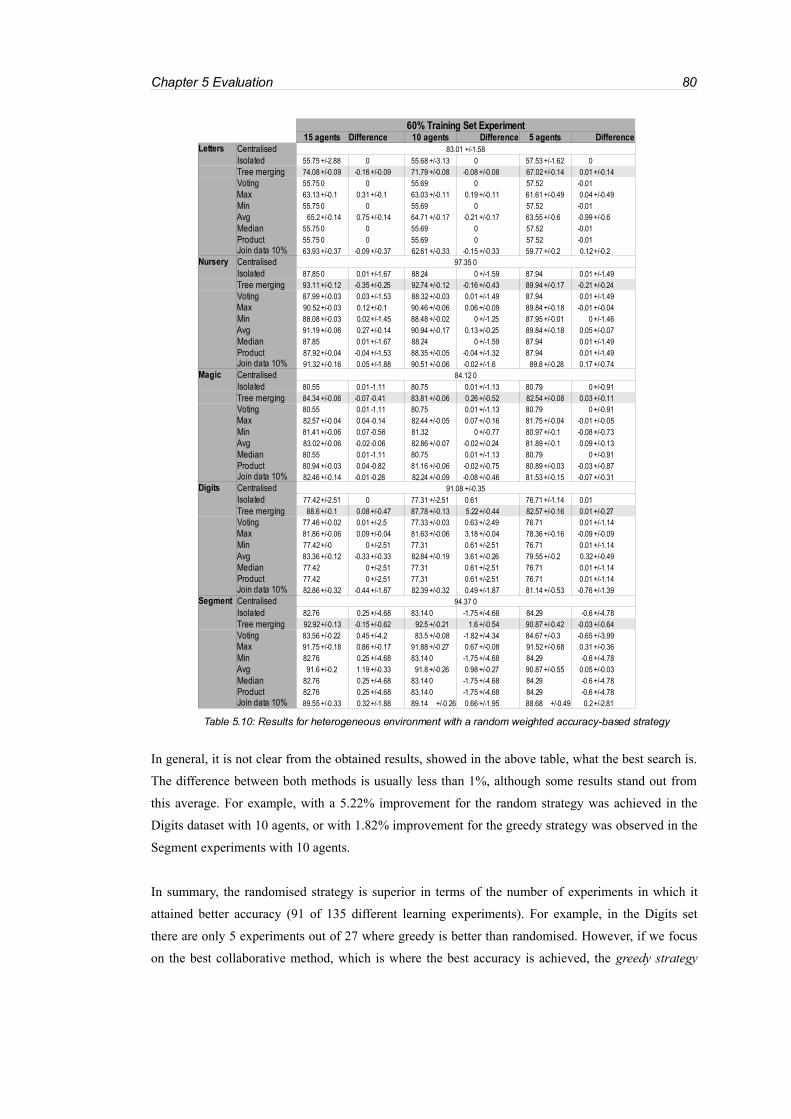
Chapter 5 Evaluation 80
In general, it is not clear from the obtained results, showed in the above table, what the best search is.
The difference between both methods is usually less than 1%, although some results stand out from
this average. For example, with a 5.22% improvement for the random strategy was achieved in the
Digits dataset with 10 agents, or with 1.82% improvement for the greedy strategy was observed in the
Segment experiments with 10 agents.
In summary, the randomised strategy is superior in terms of the number of experiments in which it
attained better accuracy (91 of 135 different learning experiments). For example, in the Digits set
there are only 5 experiments out of 27 where greedy is better than randomised. However, if we focus
on the best collaborative method, which is where the best accuracy is achieved, the greedy strategy
Table 5.10: Results for heterogeneous environment with a random weighted accuracy-based strategy
60% Training Set Experiment15 agents Difference 10 agents Difference 5 agents Difference
Letters Centralised 83.01 +/-1.58
Isolated 55.75 +/-2.88 0 55.68 +/-3.13 0 57.53 +/-1.62 0
Tree merging 74.08 +/-0.09 -0.16 +/-0.09 71.79 +/-0.08 -0.08 +/-0.08 67.02+/-0.14 0.01 +/-0.14
Voting 55.75 0 0 55.69 0 57.52 -0.0163.13 +/-0.1 0.31 +/-0.1 63.03 +/-0.11 0.19 +/-0.11 61.61 +/-0.49 0.04 +/-0.49
Min 55.75 0 0 55.69 0 57.52 -0.0165.2+/-0.14 0.75 +/-0.14 64.71 +/-0.17 -0.21 +/-0.17 63.55 +/-0.6 -0.99 +/-0.6
Median 55.75 0 0 55.69 0 57.52 -0.01
Product 55.75 0 0 55.69 0 57.52 -0.01Join data 10% 63.93 +/-0.37 -0.09 +/-0.37 62.61 +/-0.33 -0.15 +/-0.33 59.77 +/-0.2 0.12+/-0.2
Nursery Centralised 97.35 0
Isolated 87.85 0 0.01 +/-1.67 88.24 0 +/-1.59 87.94 0.01 +/-1.49Tree merging 93.11 +/-0.12 -0.35 +/-0.25 92.74 +/-0.12 -0.16 +/-0.43 89.94 +/-0.17 -0.21 +/-0.24
Voting 87.99 +/-0.03 0.03 +/-1.53 88.32+/-0.03 0.01 +/-1.49 87.94 0.01 +/-1.4990.52+/-0.03 0.12+/-0.1 90.46 +/-0.06 0.06 +/-0.09 89.84 +/-0.18 -0.01 +/-0.04
Min 88.08 +/-0.03 0.02+/-1.45 88.48 +/-0.02 0 +/-1.25 87.95 +/-0.01 0 +/-1.4691.19 +/-0.06 0.27 +/-0.14 90.94 +/-0.17 0.13 +/-0.25 89.84 +/-0.18 0.05 +/-0.07
Median 87.85 0.01 +/-1.67 88.24 0 +/-1.59 87.94 0.01 +/-1.49
Product 87.92+/-0.04 -0.04 +/-1.53 88.35 +/-0.05 -0.04 +/-1.32 87.94 0.01 +/-1.49Join data 10% 91.32+/-0.16 0.05 +/-1.88 90.51 +/-0.06 -0.02+/-1.6 89.8 +/-0.28 0.17 +/-0.74
Magic Centralised 84.12 0
Isolated 80.55 0.01 -1.11 80.75 0.01 +/-1.13 80.79 0 +/-0.91
Tree merging 84.34 +/-0.06 -0.07 -0.41 83.81 +/-0.06 0.26 +/-0.52 82.54 +/-0.08 0.03 +/-0.11Voting 80.55 0.01 -1.11 80.75 0.01 +/-1.13 80.79 0 +/-0.91
82.57 +/-0.04 0.04 -0.14 82.44 +/-0.05 0.07 +/-0.16 81.75 +/-0.04 -0.01 +/-0.05
Min 81.41 +/-0.06 0.07 -0.56 81.32 0 +/-0.77 80.97 +/-0.1 -0.08 +/-0.7383.02+/-0.06 -0.02-0.06 82.86 +/-0.07 -0.02+/-0.24 81.89 +/-0.1 0.09 +/-0.13
Median 80.55 0.01 -1.11 80.75 0.01 +/-1.13 80.79 0 +/-0.91
Product 80.94 +/-0.03 0.04 -0.82 81.16 +/-0.06 -0.02+/-0.75 80.89 +/-0.03 -0.03 +/-0.87Join data 10% 82.46 +/-0.14 -0.01 -0.28 82.24 +/-0.09 -0.08 +/-0.46 81.53 +/-0.15 -0.07 +/-0.31
Digits Centralised 91.08 +/-0.35Isolated 77.42+/-2.51 0 77.31 +/-2.51 0.61 76.71 +/-1.14 0.01
Tree merging 88.6 +/-0.1 0.08 +/-0.47 87.78 +/-0.13 5.22+/-0.44 82.57 +/-0.16 0.01 +/-0.27Voting 77.46 +/-0.02 0.01 +/-2.5 77.33 +/-0.03 0.63 +/-2.49 76.71 0.01 +/-1.14
81.86 +/-0.06 0.09 +/-0.04 81.63 +/-0.06 3.18 +/-0.04 78.36 +/-0.16 -0.09 +/-0.09
Min 77.42+/-0 0 +/-2.51 77.31 0.61 +/-2.51 76.71 0.01 +/-1.1483.36 +/-0.12 -0.33 +/-0.33 82.84 +/-0.19 3.61 +/-0.26 79.55 +/-0.2 0.32+/-0.49
Median 77.42 0 +/-2.51 77.31 0.61 +/-2.51 76.71 0.01 +/-1.14
Product 77.42 0 +/-2.51 77.31 0.61 +/-2.51 76.71 0.01 +/-1.14Join data 10% 82.86 +/-0.32 -0.44 +/-1.87 82.39 +/-0.32 0.49 +/-1.87 81.14 +/-0.53 -0.76 +/-1.39
Segment Centralised 94.37 0
Isolated 82.76 0.25 +/-4.68 83.14 0 -1.75 +/-4.68 84.29 -0.6 +/-4.78
Tree merging 92.92+/-0.13 -0.15 +/-0.62 92.5 +/-0.21 1.6 +/-0.54 90.87 +/-0.42 -0.03 +/-0.64
Voting 83.56 +/-0.22 0.45 +/-4.2 83.5 +/-0.08 -1.82+/-4.34 84.67 +/-0.3 -0.65 +/-3.9991.75 +/-0.18 0.86 +/-0.17 91.88 +/-0.27 0.67 +/-0.08 91.52+/-0.68 0.31 +/-0.36
Min 82.76 0.25 +/-4.68 83.14 0 -1.75 +/-4.68 84.29 -0.6 +/-4.7891.6 +/-0.2 1.19 +/-0.33 91.8 +/-0.26 0.98 +/-0.27 90.87 +/-0.55 0.05 +/-0.03
Median 82.76 0.25 +/-4.68 83.14 0 -1.75 +/-4.68 84.29 -0.6 +/-4.78
Product 82.76 0.25 +/-4.68 83.14 0 -1.75 +/-4.68 84.29 -0.6 +/-4.78Join data 10% 89.55 +/-0.33 0.32+/-1.88 89.14 +/-0.26 0.66 +/-1.95 88.68 +/-0.49 0.2+/-2.81
Max
Avg
Max
Avg
Max
Avg
Max
Avg
Max
Avg
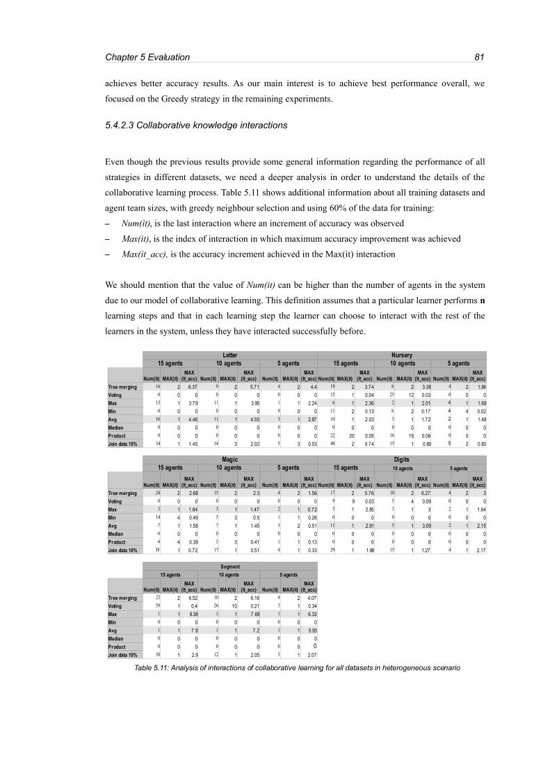
Chapter 5 Evaluation 81
achieves better accuracy results. As our main interest is to achieve best performance overall, we
focused on the Greedy strategy in the remaining experiments.
5.4.2.3 Collaborative knowledge interactions
Even though the previous results provide some general information regarding the performance of all
strategies in different datasets, we need a deeper analysis in order to understand the details of the
collaborative learning process. Table 5.11 shows additional information about all training datasets and
agent team sizes, with greedy neighbour selection and using 60% of the data for training:
– Num(it), is the last interaction where an increment of accuracy was observed
– Max(it), is the index of interaction in which maximum accuracy improvement was achieved
– Max(it_acc), is the accuracy increment achieved in the Max(it) interaction
We should mention that the value of Num(it) can be higher than the number of agents in the system
due to our model of collaborative learning. This definition assumes that a particular learner performs n
learning steps and that in each learning step the learner can choose to interact with the rest of the
learners in the system, unless they have interacted successfully before.
Table 5.11: Analysis of interactions of collaborative learning for all datasets in heterogeneous scenario
Letter Nursery15 agents 10 agents 5 agents 15 agents 10 agents 5 agents
Tree merging 16 2 6.37 9 2 5.71 4 2 4.4 19 2 3.74 8 2 3.38 4 2 1.84
Voting 0 0 0 0 0 0 0 0 0 15 1 0.04 25 12 0.03 0 0 015 1 3.79 11 1 3.95 1 1 2.24 6 1 2.36 2 1 2.01 4 1 1.69
Min 0 0 0 0 0 0 9 0 0 11 2 0.13 8 2 0.17 4 4 0.0216 1 4.46 11 1 4.55 3 1 2.87 10 1 2.03 3 1 1.72 2 1 1.48
Median 0 0 0 0 0 0 0 0 0 0 0 0 0 0 0 0 0 0
Product 0 0 0 0 0 0 0 0 0 22 20 0.05 16 15 0.06 0 0 0
Join data 10% 34 1 1.45 14 3 2.02 5 3 0.53 40 2 0.74 15 1 0.89 5 2 0.83
Magic Digits15 agents 10 agents 5 agents 15 agents 10 agents 5 agents
Tree merging 24 2 2.68 15 2 2.3 4 2 1.56 17 2 5.76 10 2 6.27 4 2 3
Voting 0 0 0 0 0 0 0 0 0 9 9 0.03 5 4 0.09 0 0 03 1 1.64 3 1 1.47 2 1 0.72 5 1 2.85 3 1 3 2 1 1.64
Min 14 4 0.49 3 3 0.5 1 1 0.26 0 0 0 0 0 0 0 0 07 1 1.58 7 1 1.45 3 2 0.51 11 1 2.91 5 1 3.09 2 1 2.15
Median 0 0 0 0 0 0 0 0 0 0 0 0 0 0 0 0 0 0
Product 4 4 0.39 3 3 0.41 1 1 0.13 0 0 0 0 0 0 0 0 0
Join data 10% 38 1 0.72 17 1 0.51 4 1 0.33 29 1 1.88 15 1 1.27 4 1 2.17
Segment
15 agents 10 agents 5 agents
Tree merging 23 2 6.52 10 2 6.16 4 2 4.07
Voting 59 1 0.4 26 10 0.21 3 1 0.341 1 8.38 1 1 7.68 1 1 6.32
Min 0 0 0 0 0 0 0 0 01 1 7.9 1 1 7.2 1 1 5.93
Median 0 0 0 0 0 0 0 0 0
Product 0 0 0 0 0 0 0 0 0Join data 10% 30 1 2.9 12 1 2.05 5 1 2.07
Num(it) MAX(it)MAX
(It_acc) Num(it) MAX(it)MAX
(It_acc) Num(it) MAX(it)MAX
(It_acc) Num(it) MAX(it)MAX
(It_acc) Num(it) MAX(it)MAX
(It_acc) Num(it) MAX(it)MAX
(It_acc)
Max
Avg
Num(it) MAX(it)MAX
(It_acc) Num(it) MAX(it)MAX
(It_acc) Num(it) MAX(it)MAX
(It_acc) Num(it) MAX(it)MAX
(It_acc) Num(it) MAX(it)MAX
(It_acc) Num(it) MAX(it)MAX
(It_acc)
Max
Avg
Num(it) MAX(it)MAX
(It_acc) Num(it) MAX(it)MAX
(It_acc) Num(it) MAX(it)MAX
(It_acc)
Max
Avg
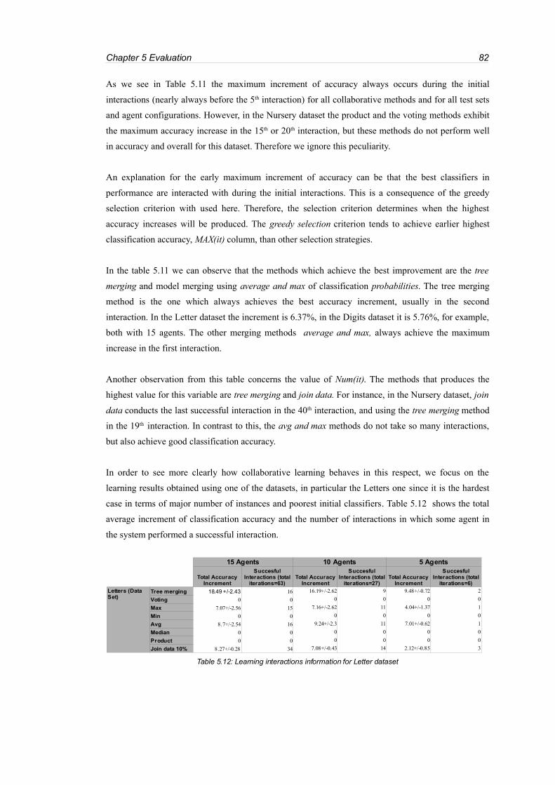
Chapter 5 Evaluation 82
As we see in Table 5.11 the maximum increment of accuracy always occurs during the initial
interactions (nearly always before the 5th interaction) for all collaborative methods and for all test sets
and agent configurations. However, in the Nursery dataset the product and the voting methods exhibit
the maximum accuracy increase in the 15th or 20th interaction, but these methods do not perform well
in accuracy and overall for this dataset. Therefore we ignore this peculiarity.
An explanation for the early maximum increment of accuracy can be that the best classifiers in
performance are interacted with during the initial interactions. This is a consequence of the greedy
selection criterion with used here. Therefore, the selection criterion determines when the highest
accuracy increases will be produced. The greedy selection criterion tends to achieve earlier highest
classification accuracy, MAX(it) column, than other selection strategies.
In the table 5.11 we can observe that the methods which achieve the best improvement are the tree
merging and model merging using average and max of classification probabilities. The tree merging
method is the one which always achieves the best accuracy increment, usually in the second
interaction. In the Letter dataset the increment is 6.37%, in the Digits dataset it is 5.76%, for example,
both with 15 agents. The other merging methods average and max, always achieve the maximum
increase in the first interaction.
Another observation from this table concerns the value of Num(it). The methods that produces the
highest value for this variable are tree merging and join data. For instance, in the Nursery dataset, join
data conducts the last successful interaction in the 40th interaction, and using the tree merging method
in the 19th interaction. In contrast to this, the avg and max methods do not take so many interactions,
but also achieve good classification accuracy.
In order to see more clearly how collaborative learning behaves in this respect, we focus on the
learning results obtained using one of the datasets, in particular the Letters one since it is the hardest
case in terms of major number of instances and poorest initial classifiers. Table 5.12 shows the total
average increment of classification accuracy and the number of interactions in which some agent in
the system performed a successful interaction.
Table 5.12: Learning interactions information for Letter dataset
15 Agents 10 Agents 5 Agents
Tree merging 18.49 +/-2.43 16 16.19+/-2.62 9 9.48+/-0.72 2
Voting 0 0 0 0 0 0
7.07+/-2.56 15 7.16+/-2.62 11 4.04+/-1.37 1
Min 0 0 0 0 0 0
8.7+/-2.54 16 9.24+/-2.3 11 7.01+/-0.62 1
Median 0 0 0 0 0 0
Product 0 0 0 0 0 0
Join data 10% 8.27+/-0.28 34 7.08+/-0.43 14 2.12+/-0.85 3
Total Accuracy Increment
SuccesfulInteractions (total
iterations=63)Total Accuracy
Increment
SuccesfulInteractions (total
iterations=27)Total Accuracy
Increment
SuccesfulInteractions (total
iterations=6)Letters (Data Set)
Max
Avg

Chapter 5 Evaluation 83
In this table we can see that in the experiments for five out of nine methods (tree merging, max, avg
and join data), the increment of accuracy achieved during learning is independent of the number of
agents configured.
The tree merging method achieves in the Letter dataset (results showed above) the best accuracy
increment in all agent scenarios (e.g. with 15 agents it achieves a 18.49% increment) while requering
a similar number of interactions as other methods such as max and avg (e.g. with 15 agents 16
interactions occur). The other methods and join data perform similarly across all scenarios (although
with 5 agents join data shows a smaller increment). However, join data requires more agent
interactions than the rest of the methods. This could be caused by the fact that transferring small parts
of data does not always allow to perform successful interactions, and therefore this learning method
tends to need more agent interactions in order to achieve a successful one (i.e. this method is weaker
in assessing the potential quality of the information that will be obtained from another agent)
Finally, we observe that an increase in the number of the agents in the system produces a gradual
increase in accuracy in the case of tree merging and join data methods. On the contrary max and avg
methods have a higher performance increment when 10 agents are present in the system.
The following figures (fig. 5.2) show three plots which present the information of the previous table
graphically. We have included the results for 15/10/5 agents, in depicting the progress of the different
learning methods.

Chapter 5 Evaluation 84
These plots show a comparison of the performance of the three learning strategies. Each plot
represents a different agent scenario, and each graph in the plots shows the accuracy progression of a
particular learning method during all its learning interactions.
In all plots we can observe that the graphs for the collaborative learning experiments are between the
Fig. 5. 2: Accuracy v. interaction count in Letters dataset

Chapter 5 Evaluation 85
centralised and distributed learning graphs as we would expect. In these plots, the highest accuracy
increment is produced by the tree merging method. The merging using average and max of
probabilities methods and the join data method have also a noticeable increment of accuracy. The
merging using min, median, and product of probabilities methods and voting method does not increase
the performance of isolated learning as presented in Table 5.8, therefore the graphs of these methods
overlap with the graph of the isolated method.
Finally the plots show that the final classification accuracy is higher when more agents are in the
system, since there is a higher possibility to perform a successful interaction with another learner and
there is more data in the system. This is analysed in more detail in the next subsection.
5.4.2.4 Increasing the number of agents
Table 5.13 summarise the effects of increasing the number of agents involved in the learning process.
For each of the best collaborative methods it shows the total increase of performance (classification
accuracy) obtained during the learning process and the index of last interaction in which an increase of
accuracy occurred.
The median, product and min methods are not shown in the above table, since no relevant variation of
accuracy was detected in any dataset.
Looking at this table, we can confirm that there is a general increase of accuracy for all the methods
appearing in the table, when we increase the number of agents in the system. When we increase the
number from five to ten agents, since in this case the increase of accuracy is the greatest. The best
results are obtained using 15 learning agents, as we can observe in the Letter and Digits experiments.
Table 5.13: Variations of accuracy when increasing the number of agents in the system
Letter Nursery Magic
5 agents 15 agents 10 agents 5 agents 15 agents 10 agents 5 agents
It It It It It It It It It
Tree merging 18.49+/-2.43 16 16.19+/-2.62 9 9.48+/-0.72 2 5.62+/-1.3 19 4.66+/-1.04 8 2.22+/-1.08 4 3.87+/-0.64 24 2.81+/-0.55 15 1.72+/-0.72 4
7.07+/-2.56 15 7.16+/-2.62 11 4.04+/-1.37 1 2.56+/-1.54 6 2.16+/-1.44 2 1.92+/-1.27 4 1.99+/-0.93 3 1.63+/-0.92 3 0.97+/-0.82 2
8.7+/-2.54 16 9.24+/-2.3 11 7.01+/-0.62 1 3.08+/-1.47 10 2.57+/-1.17 3 1.86+/-1.24 2 2.5+/-0.99 7 2.14+/-0.82 7 1.01+/-0.68 3
Join data(0.1) 8.27+/-0.28 33 7.08+/-0.43 14 2.12+/-0.85 3 3.43+/-0.37 40 2.29+/-0.07 15 1.7+/-0.47 5 1.93+/-0.69 38 1.58+/-0.58 17 0.81+/-0.45 4
Digits Segment
15 agents 10 agents 5 agents 15 agents 10 agents 5 agents
It It It It It It
Merge Tree 11.1+/-1.94 17 10.88+/-1.46 10 5.86+/-0.71 4 10.56+/-3.93 23 9.45+/-3.57 10 6.01+/-3.72 4
4.35+/-2.41 5 4.36+/-2.17 3 1.75+/-0.89 2 8.38+/-4.33 1 7.68+/-3.78 1 6.32+/-4.46 1
6.27+/-2.06 11 6.03+/-2.27 5 2.53+/-0.45 2 7.9+/-4.15 1 7.2+/-3.55 1 5.93+/-4.26 1
Join data(0.1) 5.88+/-0.32 29 5.69+/-0.95 15 5.2+/-0.78 4 6.72+/-2.47 30 5.54+/-2.64 12 3.59+/-1.48 5
15 agentsents10 agentsents
Inc Inc Inc Inc Inc Inc Inc Inc Inc
Max
Avg
Inc Inc Inc Inc Inc Inc
Max
Avg

Chapter 5 Evaluation 86
The increase of agents comes with an increase of new potential interactions with different agents,
which may induce better accuracy results. However, not all methods achieve the same performance
improvement nor do they use the same number of interactions as we have seen in the above analysis.
In this respect, join data is the method which needs the highest number of interactions, and it is not the
best in terms of accuracy. Tree merging is the method which achieves the highest performance increase
for all scenarios using a similar number of interactions while performing better than max and avg.
Figure 5.3 shows the variations of the performance average for all the different strategies and for all
agent configurations. This figure is similar to the 5.1 but for an heterogeneous scenario.
The classification performance of the three learning strategies is summarised in the above plot. With
respect to collaborative learning, the method with best results in accuracy (Tree merging) is only
shown. Distributed isolated learning is substantially outperformed by collaborative agent learning, for
instance in the Letter and Segment datasets. Furthermore, the collaborative learning method achieves
a classification accuracy nearly equivalent to that achieved by the centralised strategy in most of the
datasets and especially in scenarios with 15 agents. Regarding the Segment and Magic datasets, in the
best case the collaborative learning achieves better accuracy than centralised learning.
Increasing the number of learners does not produce any increment in accuracy in centralised learning
as there is only a single agent using the data. In terms of distributed isolated learning there is no
noticeable increment in accuracy, since by definition in this experiment (section 4.4.2.4) the dataset
Fig. 5. 3: Comparison of different agent configurations

Chapter 5 Evaluation 87
partitions have a predefined size, and therefore adding new partitions and building the corresponding
classifiers does not lead to a great increment in average of the classification performance in the group
of classifiers. However, for the collaborative solution, a gradual gain in the average accuracy is
produced when the number of agents is increased. This situation can be observed in all five datasets,
but is more noticeable in the Letter dataset.
5.4.2.5 Increasing of training dataset in collaborative agent learning
As far as the effect of increasing the amount of training data in the learning strategies is concerned,
the next plot (Fig.5.4) presents the gain in accuracy for all agent configurations (15/10/5) and for all
datasets using 80% of all data for training the classifier (20% more than in the previous experiments).
In the above plot the classification performance of the three learning strategies is presented. For
collaborative learning, the method with the best results in terms of accuracy (tree merging) is shown
for ease of readability. If we compare this picture with the experiments using 60% of data for training
(fig 5.3), no great difference can be observed. Slightly better performance is generally achieved in
terms of accuracy, especially for the Letter, Digits and Segment datasets.
Increasing the number of learners, as commented in 5.4.2.4, does not produce any increment in
accuracy in centralised learning and no noticeable increment in accuracy in the distributed isolated
Fig. 5.4: Comparison of learning method performance when size of training sets is
increased

Chapter 5 Evaluation 88
learning case. However, for the collaborative method, a substantial gain in the average accuracy is
produced in all five datasets. This is most noticeable in the Letter and Digits datasets.
Regarding increases in the size of the training set, Table 5.14 shows the difference in accuracy after an
increment of 20% of training data for all datasets. In this table we have omitted the voting, median,
product and min methods because they do not exhibit any significant gain in classification accuracy.
Looking at the above table, we can confirm that there is a general increase of classification accuracy
for all datasets when the training set of the classifiers is increased. However, for centralised and
distributed isolated learning, a slight deterioration in average accuracy in distributed learning occurs
for the Segment dataset with five agents.
With respect to the collaborative learning experiments, a general improvement of accuracy is observed
when the training data is increased. However, for the Segment and Digits sets the accuracy decreases,
e.g. In the Segment set with five agents it decreases by 3%. This fact must be a result of the obtained
classifiers having worse performance than the ones in the 60% of the training data.
Regarding the number of agents, there is not a clear tendency that increasing the number of agents
will affect accuracy in a positive way, e.g. in the experiments where better results are observed when
increasing the number of agents from five to fifteen agents in the Nursery and Magic sets, or from five
to ten agents in the Nursery, Magic, and Digits sets.
Finally, we can see that there is not a best single method with respect to performance increase. Results
depend on the dataset. Although tree merging is the method which achieves the highest accuracy, it is
not always the best method in terms of accuracy increment. When using 20% more data for training,
other methods outperform this accuracy increment, such as max and avg. This is observable for
Table 5.14: Variation of accuracy when increasing training sets from 60% to 80% of all available data
Letter Nursery Magic
15 agents 10 agents 5 agents 15 agents 10 agents 5 agents 15 agents 10 agents 5 agents
Centralized 1.54 +/-0.93 0.4 +/-0.09 0.44 +/-0.44
Isolated 3.86 +/-0.38 3.8 +/-0.77 1.45 +/-0.46 0.91 +/-0.22 0.88 +/-0.06 1.55 +/-0.19 0.57 +/-0.29 0.65 +/-0.38 0.36 +/-0.1
Tree merging 1.44 +/-0.05 1.86 +/-0.04 1.16 +/-0.08 1.27 +/-0.01 0.8 +/-0.22 2.15 +/-0.44 0.31 +/-0.19 1.05 +/-0.28 1.16 +/-0.08
3.04 +/-0.01 2.31 +/-0.06 1.5 +/-0.34 2.06 +/-0.15 1.31 +/-0.06 1.94 +/-0.06 0.37 +/-0.02 0.65 0 0.93 +/-0.23
3.77 +/-0.2 1.94 +/-0.19 0.33 +/-0.28 1.54 +/-0.13 0.88 +/-0.29 1.91 +/-0.13 0.19 +/-0.03 0.6 +/-0.22 0.74 +/-0.01
Join data 10% 2.54 +/-0.32 2.43 +/-0.43 2.47 +/-0.4 1.01 +/-0.06 1.21 +/-0.02 1.55 +/-0.53 0.36 +/-0.14 0.25 +/-0.16 0.34 +/-0.13
Digits Segment
15 agents 10 agents 5 agents 15 agents 10 agents 5 agents
Centralized 2.93 +/-0.1 1.01 +/-0.03
Isolated 2.76 +/-0.48 1.35 +/-1.01 1.76 +/-0.95 2.91 +/-1.55 2.19 +/-0.63 -0.48 +/-0.2
Tree merging 3.59 +/-0.05 -1.12 +/-0.01 2.37 +/-0.19 0.35 +/-0.09 -0.74 0 -1.9 +/-0.22
6.13 +/-0.19 0.03 +/-0.12 2.99 +/-0.23 -0.65 +/-0.33 -2.14 +/-0.11 -3.16 +/-0.09
4.17 +/-0.01 -1.1 +/-0.37 2.38 +/-0.12 0.07 +/-0.14 -0.48 +/-0.32 -2.77 +/-0.14
Join data 10% 2.99 +/-0.47 1.85 +/-0.25 0.47 +/-0.27 1.24 +/-0.86 0.97 +/-0.02 -0.52 +/-0.92
Max
Avg
Max
Avg
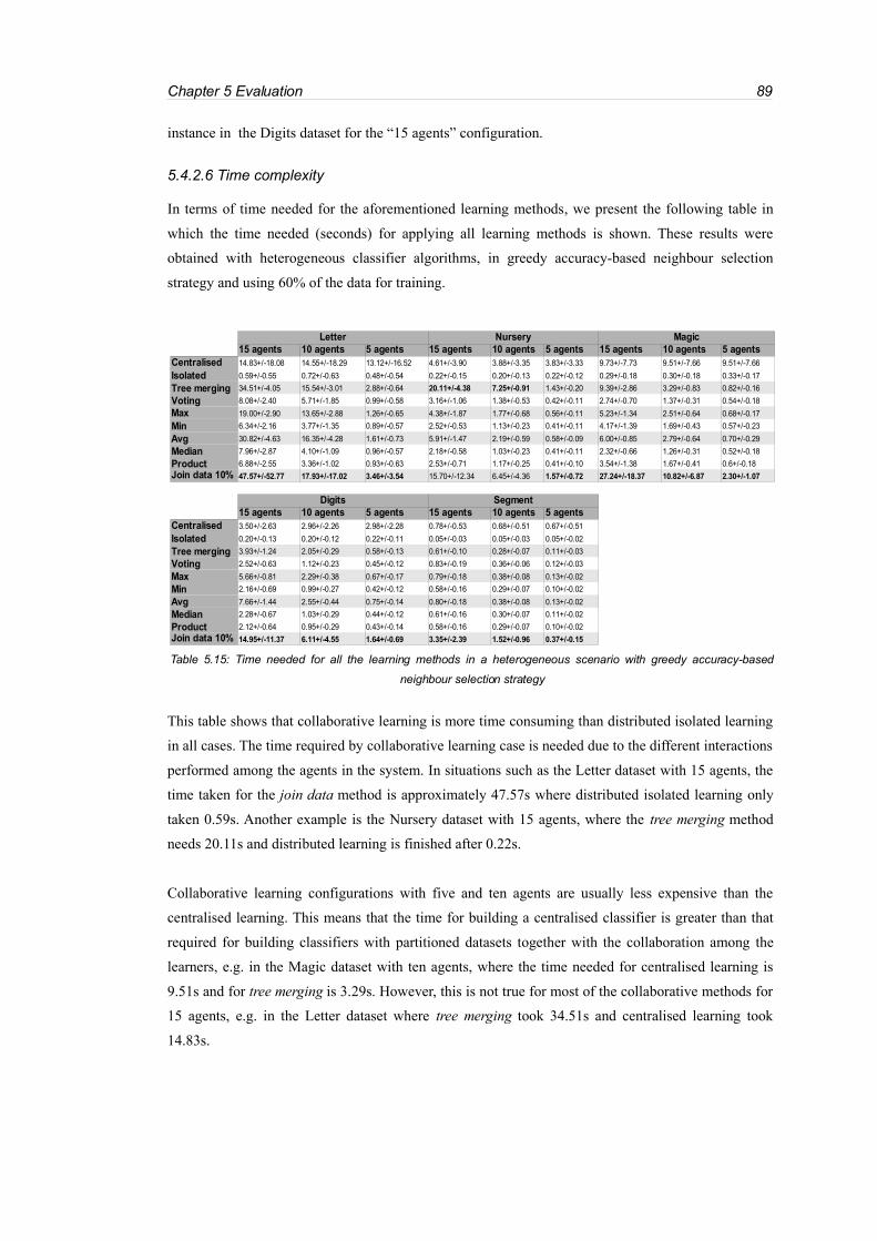
Chapter 5 Evaluation 89
instance in the Digits dataset for the “15 agents” configuration.
5.4.2.6 Time complexity
In terms of time needed for the aforementioned learning methods, we present the following table in
which the time needed (seconds) for applying all learning methods is shown. These results were
obtained with heterogeneous classifier algorithms, in greedy accuracy-based neighbour selection
strategy and using 60% of the data for training.
This table shows that collaborative learning is more time consuming than distributed isolated learning
in all cases. The time required by collaborative learning case is needed due to the different interactions
performed among the agents in the system. In situations such as the Letter dataset with 15 agents, the
time taken for the join data method is approximately 47.57s where distributed isolated learning only
taken 0.59s. Another example is the Nursery dataset with 15 agents, where the tree merging method
needs 20.11s and distributed learning is finished after 0.22s.
Collaborative learning configurations with five and ten agents are usually less expensive than the
centralised learning. This means that the time for building a centralised classifier is greater than that
required for building classifiers with partitioned datasets together with the collaboration among the
learners, e.g. in the Magic dataset with ten agents, where the time needed for centralised learning is
9.51s and for tree merging is 3.29s. However, this is not true for most of the collaborative methods for
15 agents, e.g. in the Letter dataset where tree merging took 34.51s and centralised learning took
14.83s.
Table 5.15: Time needed for all the learning methods in a heterogeneous scenario with greedy accuracy-based
neighbour selection strategy
Letter Nursery Magic15 agents 10 agents 5 agents 15 agents 10 agents 5 agents 15 agents 10 agents 5 agents
Centralised 14.83+/-18.08 14.55+/-18.29 13.12+/-16.52 4.61+/-3.90 3.88+/-3.35 3.83+/-3.33 9.73+/-7.73 9.51+/-7.66 9.51+/-7.66
Isolated 0.59+/-0.55 0.72+/-0.63 0.48+/-0.54 0.22+/-0.15 0.20+/-0.13 0.22+/-0.12 0.29+/-0.18 0.30+/-0.18 0.33+/-0.17
Tree merging 34.51+/-4.05 15.54+/-3.01 2.88+/-0.64 20.11+/-4.38 7.25+/-0.91 1.43+/-0.20 9.39+/-2.86 3.29+/-0.83 0.82+/-0.16
Voting 8.08+/-2.40 5.71+/-1.85 0.99+/-0.58 3.16+/-1.06 1.38+/-0.53 0.42+/-0.11 2.74+/-0.70 1.37+/-0.31 0.54+/-0.18
19.00+/-2.90 13.65+/-2.88 1.26+/-0.65 4.38+/-1.87 1.77+/-0.68 0.56+/-0.11 5.23+/-1.34 2.51+/-0.64 0.68+/-0.17
Min 6.34+/-2.16 3.77+/-1.35 0.89+/-0.57 2.52+/-0.53 1.13+/-0.23 0.41+/-0.11 4.17+/-1.39 1.69+/-0.43 0.57+/-0.23
30.82+/-4.63 16.35+/-4.28 1.61+/-0.73 5.91+/-1.47 2.19+/-0.59 0.58+/-0.09 6.00+/-0.85 2.79+/-0.64 0.70+/-0.29
Median 7.96+/-2.87 4.10+/-1.09 0.96+/-0.57 2.18+/-0.58 1.03+/-0.23 0.41+/-0.11 2.32+/-0.66 1.26+/-0.31 0.52+/-0.18
Product 6.88+/-2.55 3.36+/-1.02 0.93+/-0.63 2.53+/-0.71 1.17+/-0.25 0.41+/-0.10 3.54+/-1.38 1.67+/-0.41 0.6+/-0.18
Join data 10% 47.57+/-52.77 17.93+/-17.02 3.46+/-3.54 15.70+/-12.34 6.45+/-4.36 1.57+/-0.72 27.24+/-18.37 10.82+/-6.87 2.30+/-1.07
Digits Segment15 agents 10 agents 5 agents 15 agents 10 agents 5 agents
Centralised 3.50+/-2.63 2.96+/-2.26 2.98+/-2.28 0.78+/-0.53 0.68+/-0.51 0.67+/-0.51
Isolated 0.20+/-0.13 0.20+/-0.12 0.22+/-0.11 0.05+/-0.03 0.05+/-0.03 0.05+/-0.02
Tree merging 3.93+/-1.24 2.05+/-0.29 0.58+/-0.13 0.61+/-0.10 0.28+/-0.07 0.11+/-0.03
Voting 2.52+/-0.63 1.12+/-0.23 0.45+/-0.12 0.83+/-0.19 0.36+/-0.06 0.12+/-0.03
5.66+/-0.81 2.29+/-0.38 0.67+/-0.17 0.79+/-0.18 0.38+/-0.08 0.13+/-0.02
Min 2.16+/-0.69 0.99+/-0.27 0.42+/-0.12 0.58+/-0.16 0.29+/-0.07 0.10+/-0.02
7.66+/-1.44 2.55+/-0.44 0.75+/-0.14 0.80+/-0.18 0.38+/-0.08 0.13+/-0.02
Median 2.28+/-0.67 1.03+/-0.29 0.44+/-0.12 0.61+/-0.16 0.30+/-0.07 0.11+/-0.02
Product 2.12+/-0.64 0.95+/-0.29 0.43+/-0.14 0.58+/-0.16 0.29+/-0.07 0.10+/-0.02
Join data 10% 14.95+/-11.37 6.11+/-4.55 1.64+/-0.69 3.35+/-2.39 1.52+/-0.96 0.37+/-0.15
Max
Avg
Max
Avg
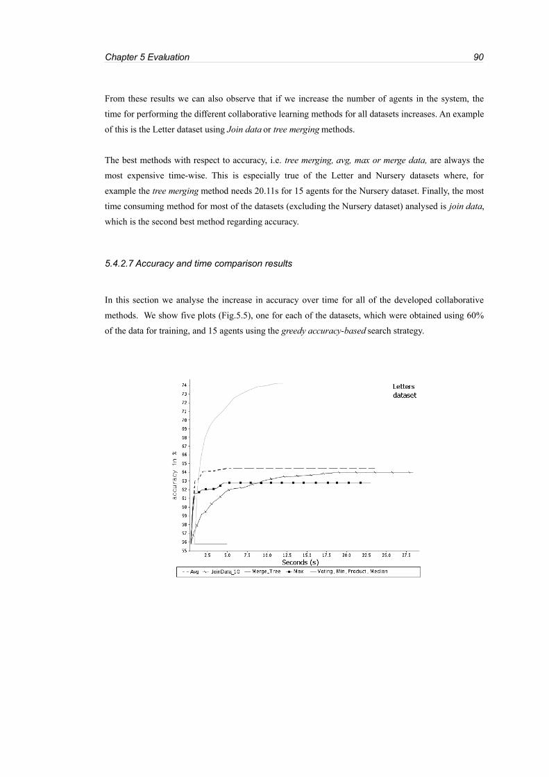
Chapter 5 Evaluation 90
From these results we can also observe that if we increase the number of agents in the system, the
time for performing the different collaborative learning methods for all datasets increases. An example
of this is the Letter dataset using Join data or tree merging methods.
The best methods with respect to accuracy, i.e. tree merging, avg, max or merge data, are always the
most expensive time-wise. This is especially true of the Letter and Nursery datasets where, for
example the tree merging method needs 20.11s for 15 agents for the Nursery dataset. Finally, the most
time consuming method for most of the datasets (excluding the Nursery dataset) analysed is join data,
which is the second best method regarding accuracy.
5.4.2.7 Accuracy and time comparison results
In this section we analyse the increase in accuracy over time for all of the developed collaborative
methods. We show five plots (Fig.5.5), one for each of the datasets, which were obtained using 60%
of the data for training, and 15 agents using the greedy accuracy-based search strategy.

Chapter 5 Evaluation 91

Chapter 5 Evaluation 92
Fig. 5.5: Increase of accuracy over time for all datasets
These graphs represent the time and the accuracy obtained for each of the learning methods in the
different datasets. We can observe that some experiments take more time for concluding their learning
(longer graphs) than others. The learning is concluded once the termination criterion is satisfied, in
this case once 60% of the learning interactions are performed.
In this terms, the best method by far regarding accuracy for all plots is the tree merging method, which
at the same time is not always the most time-demanding, e.g. in the Digits or Letters plots. The worst
methods are voting, product, median and min which usually are the least time consuming, e.g. in the
Magic dataset. The most costly method is join data, except for the Nursery dataset. Moreover, we can
see that the method which needs most time to perform its learning is not always the one that has the
highest accuracy, as can be observed in the Magic, Digits or Segment experiments.
Finally, we emphasise average and max methods as the ones which usually achieves in the least time a
relatively high classification accuracy improvement. This is specially observable in Segment or
Nursery datasets. However, these methods never reach the accuracy of the tree merging method. The
tree merging method achieves a great increase of accuracy in a little time for all datasets, e.g. in the
Segment dataset. However, this method takes more time to complete than the other efficient
collaborative methods (average or max). This is obvious, for example, in the Nursery dataset. On the
other hand, the Join data method is the slowest in terms of learning for all datasets, but at the same
time it slightly and progressively increases its accuracy along the learning process.
Chapter 5 Evaluation 93
5.5 Conclusions from the results
As mentioned in chapter 1, our research focuses on proposing a solution for improving classification
in distributed data mining environments where the possibilities of data transfer are limited. Therefore,
we developed a collaborative agent-based learning model (chapters 3 and 4) in which the different
agents transfer and integrate learning knowledge (such as outputs, models or small quantities of data)
with other agents in the system.
The present chapter has presented the results of an extensive evaluation of the collaborative learning
strategy. In the following sections, we attempt to extract some conclusions from these results. Firstly,
we present some general comments regarding centralised and distributed isolated strategies, and then
we look at details of the collaborative distributed strategy.
5.5.1 General aspects of different learning strategies
The centralised and distributed isolated learning strategies were tested in order to allow for a
comparative evaluation of the suggested collaborative learning strategy (sections 5.4.1 and 5.4.2). The
results obtained through experimentation showed that the best performance was achieved by
centralised learning. This is not a surprise as this strategy uses all the training data available for
learning, and therefore has an advantage over all other strategies, and this explains the strategy’s
results in classification accuracy, which are almost always superior to all alternatives.
On the contrary, the results obtained using the distributed isolated learning methods were the poorest
regarding classification performance. This was not surprising since this strategy (section 4.4.2.2)
builds the classifiers from partitions of all the data available and does not perform any collaboration
on the partial results of the individual classifiers. Two factors related to classification accuracy were
identified in the evaluation of this strategy. Firstly, an increase in the number of agents affects the
average of the individual classification accuracies, since new classifiers from different partitions are
introduced to the system. Secondly, an increase in the size of the data partitions improves the
classification accuracy of the classifiers by making more knowledge available to the individual
learners.
5.5.2 General aspects of collaborative learning
In general terms, we observed that collaboration substantially improves the classification performance
of distributed learners for most of the tested collaborative integration methods and in different
Chapter 5 Evaluation 94
scenarios, e.g. for different numbers of agents, data training sizes, datasets, classifier types or agent
selection strategies. Furthermore, in most of the evaluated scenarios, the performance achieved by the
collaborative strategy was similar to that obtained using the centralised learning method (section 5.4),
and this was particularly the case when using the tree merging integration method. This method
managed to produce better results compared with the centralised learning solution in certain scenarios.
This illustrates the potential for collaboration among the learning processes and, in particular, for the
use of our agent learning model for distributed environments with limited data sharing.
One of the parameters that positively influenced the performance of the collaborative learning was the
use of distinct classification algorithms for building the classifiers (heterogeneous scenario). This was
shown in section 5.4.2.1, in which the collaborative learning experimental results from homogeneous
scenarios were compared with results obtained in heterogeneous scenarios. From these results, we
concluded that the performance of the classifiers in heterogeneous scenarios was superior to
classification performance in homogeneous scenarios. A possible reason for this is given in [29] where
the authors explain that heterogeneity in classification algorithms entails less correlated classifiers
(classifiers that do not agree in misclassification of samples). Having weakly correlated classifiers
means having different data representations, and merging different representations may lead to better
classification rates as merged models cover different aspects of the learning problem, which may be
hard to represent when using only one type of algorithm.
Another observation extracted from the results was that the greedy accuracy-based neighbour selection
strategy (section 5.4.2.2) allows the agent to achieve high classification performances in early
interactions. A plausible reason for this is that the best classifiers regarding classification accuracy are
selected to begin with, based on the assumption that the interactions with classifiers with good
performance tends to produce accurate merged models. Another learner selection criterion was
evaluated as well, the randomised weighted selection strategy. This criterion is different from the
greedy one, as it uses a randomised method for selecting the neighbour to interact with. In section
(5.4.2.3) we observed that, in the long term, results similar to the greedy method (with a difference of
less than 1%) were achieved. Overall, the greedy strategy is preferable, since this selection strategy
allows higher accuracies in the short term and, since in the scenario with fifteen agents (where the
highest classification accuracy was achieved), this strategy nearly always achieves better results than
the randomised one.
Some further conclusions can be drawn from the evaluation of the collaborative methods (sections
5.4.1 and 5.4.2) :
– The best collaborative method in terms of classification accuracy improvement was the tree
merging operation. This is the novel method developed specifically for our research (colTree) and

Chapter 5 Evaluation 95
consists of integrating predictive tree-based models from different agents. A possible explanation
for the outstanding results of this method can be found in the definition of the operation which
always attempts to identify the interesting parts of the selected learner’s model and to integrate it
with the learning agent’s current model. These promising results are indicative of the potential of
this technique and are encouraging for future research on the topic.
– With respect to the evaluation of the knowledge integration operations based on output merging,
the best ones were avg (or sum) and max operations using posterior probabilities. These methods
increase the initial accuracy of the distributed isolated learners substantially for all datasets, but
they do not improve on the results achieved by the tree merging operation. These methods were
extensively tested and analysed in previous studies and positive results have been obtained before
[29,30]. Previous studies justify the good performance of the classifier merging methods (avg and
max ) since these do not amplify the classification errors like other algebraic merging operations
(i.e. product), and this makes these methods resilient to estimation errors.
Some other integration methods based on outputs were tested, such as voting, min, median and
product. These didn’t perform well in the collaborative setup, and most of the time they did not
improve over their initial classification accuracy. A reason for the poor performance of the voting
and median methods is that these prefer the prediction of the current classifier rather than the
opinions of the classifier that, by definition, they are going to be integrated with. Therefore, no
increment in accuracy is obtained. On the other hand, the fact that min and product operators did
not perform better was quite unexpected. This was also observed in [29,30] where it was
suggested that this is because these methods are very sensitive to errors. For example, if a
classifier reported a zero as a posterior probability for the correct class, the probability output
would be zero for this class after the min and product operation and, therefore, the correct class
would not be identified. Therefore, no classification performance increase would be achieved in
such cases.
– Integration operation based on exchanging data was also tested. When using this method, small
quantities of training data are sent from the selected agent to the learning agent. This merging
operation performs well in the collaborative model because adding new training data helps in
obtaining better classifiers. However, these results were not as promising as those achieved by
tree-based model merging or output merging.
Another conclusion drawn from the results was that applying collaborative learning to a higher
number of agents in the system produced more accurate classifiers. An example for this is given in
section 5.4.2.3 where the best performance for collaborative learning was always achieved with the
largest agent set (15 agents). An explanation for this is that having more agents permits having more
interactions, and, therefore, more possibilities to achieve successful knowledge integration (classifier
Chapter 5 Evaluation 96
interactions which produce a new and more accurate classifier). The best collaborative method after
the increase in the number of agents is still the same, that is the tree merging. Other methods which
also showed good performance when number of agent is increased were still the same as before: max,
avg and join data.
Furthermore, we can infer from the experiments that collaborative learning achieves a general
improvement in classification accuracy when the data used for training is increased by 20%. This is
because all classifiers have more data for training than before. The best method in terms of accuracy
obtained after the increase of data is still tree merging, and the other comparable methods are still the
same: avg and max and join data. Moreover, the methods that do not show a substantial increase in
accuracy are also still the same: voting, min, median and product.
Experiments were also conducted to evaluate the time needed for performing collaborative learning.
From these experiments we found out that the following parameters strongly influence the time
related performance of collaborative learning (section 5.4.2.6):
– The collaborative integration method. Merging data requires that the learners transfer the data and
retrain their classifiers for obtaining new ones. These processes are more costly than other
methods, such as those based on merging posteriori probabilities which only send models (or
results, depending on the implementation) and perform simple algebraic operations to obtain the
overall classification.
– The number of agents in the system. The more agents, the more communication is needed and
this is especially the case for selection where the agents have to find the best neighbour to interact
with.
– The size of the training set. Using more instances for training leads to spending more time on
processing them during the construction of the classifier.
– The classification technique. The classification technique makes use of different internal
operations for building a classifier, and each technique requires different amounts of time for this
process. Furthermore, each technique builds a different type of classifier, and the time needed for
classification depends on the representation used.
The time required for the distributed isolated strategy is obviously less than that needed for
collaboration. Regarding the different collaborative methods (section 5.4.2.7), the most time
consuming was the join data method for most of the datasets, although this method does not exhibit
the best performance. The least expensive methods in terms of time were those based on merging
probabilities since these methods only perform simple mathematical operations for merging results,
and those which had the worst classification accuracy improvements (i.e. voting, product, median and
min) were particularly fast since they do not have to spend time on updating the learner's model. The

Chapter 5 Evaluation 97
remaining methods i.e. tree merging, max and avg can be recommended as they showed a good
classification improvement and were not the most time consuming.
We also evaluated collaborative learning methods in terms of learning speed (section 5.4.2.7).
Learning speed refers to the value of classification accuracy improvement over time. The fastest
methods observed from the results were avg and max, since they achieved the highest accuracy in the
least amount of time, as compared with the other methods. The tree merging method was slightly
slower than the previous methods, but it eventually achieved higher classification accuracy for all
datasets. The reasons explaining this behaviour is that the best classifiers in terms of accuracy are the
first to be merged. This is due to the greedy accuracy-based neighbour selection criterion. The fact that
the collaborative learning strategy has a high learning rate, is a strong result since it offers the
possibility of implementing efficient systems, in which it takes little time for the performance of the
classifiers in the system to improve significantly.
The collaborative learning strategy can be easily scaled by adding new agents in the system, since the
methods and processes used in the collaborative model can deal with an arbitrary number of agents in
the system. However, agent scalability is limited by two factors: the increase of the time needed for
learning and possible network overloading. The main reason for this is that including more agents
implies more communication between them. In particular, every time an agent attempts to perform a
new learning step, it would broadcast its request to the rest of the agents, in order to find the most
interesting agent to interact with. However, we managed to reduce this cost by including some
filtering processes in the learning model (section 3.4.1), in order to communicate only with
appropriate agents. Another possible reason for network overloading is the knowledge exchange
among agents. We proposed different alternative strategies in order to reduce this cost. One of them
was communication of small quantities of training data (which, as we have seen, is the most time-
consuming and is not optimal in terms of performance improvement). Another method to limit
communication was output merging, which could be implemented for transferring models instead of
outputs, thus saving time and reducing network load. This method achieved good performance with
relatively limited computational effort. Finally, we developed another alternative which also consisted
of transferring models among learners (and therefore even less communication than the previous one),
where each learner merges the received models using an internal process which, while requiring
slightly more time than that required by the previous method, achieves much higher classification
accuracy, almost as high as (or higher than) that achieved using a centralised learning strategy.
Finally, the collaborative model can also scale in terms of new data for training or for testing. Adding
new data for training does not cause higher network load; however, it would result in an increase of
the initial time needed for building the classifiers for any learning strategy. Furthermore, it would have
consequences for the collaborative learning method based on data merging. This method needs to

Chapter 5 Evaluation 98
build the classifier every time new data is obtained. Therefore, this method would be slowed down
when using more data. Additionally, tree merging would require more time as it uses the training set
for identifying the interesting parts of the selected learner's model. The other methods, i.e. merging
probabilities or predicted labels, do not make use of the training data, therefore adding training data
would not cause higher time complexity. In case more data is provided for testing, clearly more time
would be needed for all the methods in general, since the evaluation would require more time as more
instances would have to be processed.

Chapter 6 Conclusions and further work 99
Chapter 6
Conclusions and further work
The main objective of this project has been to investigate whether collaboration in distributed data
mining environments is feasible and advantageous. In particular, our focus has been on systems
composed of interconnected local nodes, in which the local classification learning task (learner) is
performed in environments, with limited data transfer due to legal, security or economic reasons.
Our approach adopted the notions of autonomy and collaboration from a previous agent-based
learning framework [1], and proposed a collaborative agent-based learning model that redefines and
extends the learning steps defined in the previous framework for limited data environments. In
particular, four well-defined stages have been identified for the collaborative learning step: neighbour
selection, knowledge integration, evaluation and learning update. For each of the different steps, we
have proposed concrete methods and some possible alternatives for further research.
The most significant element of our architecture is knowledge learning integration since this is the
phase where the process of integrating the knowledge of two learners is performed. The integration
problem has been investigated by looking at two kinds of learning societies. The first is composed of
homogeneous learners that use the same type of learning algorithm, whereas the second is comprised
of agents using heterogeneous learning algorithms. In each type of society, three different types of
learning knowledge were considered for integration: training data, classification outputs and
hypotheses. For each of these types of knowledge and for each type of society, we defined different
integration operations, such as merging small quantities of data, majority predicted class voting, or
maximum, minimum, average, product and sum of posterior probability estimates. In addition we
propose ColTree as a new operator for integrating heterogeneous learning models based on decision
trees. ColTree not only provides a common schema to translate different decision trees, but also
permits integrating them and performing classifications using the resulting integrated model. This
integration operation is concerned with the selection of the most interesting tree branches of the model
to integrate with, and defines a process for eliminating the redundancies from the resulting model. The
classification process performs a classification with the different branches of the merged tree, and
unifies the different opinions using a majority voting mechanism. This technique was successfully
implemented and evaluated for SimpleCart, BFtree and REPTree Weka tree classifiers.

Chapter 6 Conclusions and further work 100
Moreover, we have provided an evaluation of the proposed agent-based collaborative learning model.
An application has been designed that is flexible enough to allow for testing our model in different
learning environment configurations, incorporating different numbers of agents, different dataset sizes
and distinct dataset partition sizes. Furthermore, different learning experiments of the collaborative
model can be configured to specify any of the created methods for each of the procedural components
of the model.
The empirical investigation indicates that for most of the configurations of the collaborative learning
experiments, the local learners improve their initial classification accuracy and achieve classification
accuracies close to the centralised solution (the omniscient strategy that uses all domain data for the
classifier learning). The best results were obtained using the ColTree tree-based model merging
operation. This method even outperformed the classification performance achieved by the centralised
solution in a couple of scenarios.
Some other conclusions were obtained through experimentation with the collaborative learning model.
In particular, we discovered that this learning model is efficient in terms of learning speed, since the
learners attain high performance improvements within a limited amount of time during the initial
interactions (especially using the greedy neighbour selection technique and the output and model
merging operations). Another interesting observation from the experimentation was that collaborative
learning achieves better performance improvements in heterogeneous environments with large
numbers of agents.
This model still presents significant potential for further research. For example, with respect to the
neighbour selection criterion, more advanced search techniques could be defined for improving the
learning speed of the learners. New complex measurements could be added in the update criterion for
improving the quality of the resulting learners. New methods for merging operations could be
investigated, especially in hypothesis merging since the most relevant results have been obtained
through this technique. Finally, although the methods and processes created for the collaborative
model can deal with an arbitrary number of agents in the system, or with the addition of new data for
training without causing higher network load, exhaustive tests should be conducted in order to
evaluate the performance and the time-cost of the different collaborative methods in large-scale
systems.

Bibliography 101
Bibliography
[1] J. Tozicka, M. Rovatsos, M.A. Pechoucek. A Framework for Agent-Based Distributed Machine
Learning and Data Mining. In Proceedings of the Sixth International Joint Conference on Autonomous
Agents and Multiagent Systems, Honolulu, Hawaii, USA , 2007. Pp. 666-673. ACM Press.
[2] P. Stone and M. Veloso. Multiagent Systems: A Survey from a Machine Learning Perspective,
Autonomous Robots, vol. 8, no. 3, pp. 345–383, 2000.
[3] M. Wooldridge and N. Jennings. Intelligent Agents: Theory and Practice. The Knowledge
Engineering Review, vol. 10, no. 2, pp. 115–152, 1995.
[4] M. Wooldridge. An introduction to multiagent systems. Wiley, 2002.
[5] G. Weiss (editor). Multiagent Systems: A Modern Approach to Distributed Artificial Intelligence.
The MIT Press, Cambridge, MA. 2000.
[6] S. Russell and P. Norvig. Artificial intelligence: a modern approach. Prentice-Hall, Englewood
Cliffs, NJ, 1995.
[7] M. Klusch, S. Lodi, and G. Moro. Agent-Based Distributed Data Mining: The KDEC scheme. In
AgentLink, LNCS 2003. Number 2586, pp. 104-122. Springer.
[8] T.G. Dietterich. An experimental comparison of the three methods for constructing ensembles of
decision trees: Bagging, boosting and randomization. Machine Learning, 2000. Vol. 40, no. 2, pp. 139–
157.
[9] J.Widom. Research Problems in Data Warehousing. In Proceedings of fourth International
Conference on Information and Knowledge Management. Baltimore, MD. Nov. 1995, pp. 25-30.
ACM press.
[10] J.R. Quinlan, Generating Production Rules from decision trees. Proceedings of the Tenth
International Joint Conference on Artificial Intelligence, 1987, pp. 304-307. Morgan Kaufmann

Bibliography 102
Publishers.
[11] L.I. Kuncheva. Combining pattern classifiers: methods and algorithms. Wiley, 2004
[12] P. Chan and S. Stolfo Experiments on multistrategy learning by metalearning. Proceedings of the
Second International Conference on Information and Knowledge Management, Washington, DC,
USA, November 1-5, 1993. Pp. 314-323. ACM Press.
[13] H. Kargupta et al. Collective principal component analysis from distributed, heterogeneous data
using an agent-based architecture. Workshop on Large-Scale Parallel KDD Systems, SIGKDD,
August 15, 1999, San Diego,CA, USA. Principles of Data Mining and Knowledge Discovery. Lecture
Notes in Computer Science. Vol. 1910. Springer.
[14] W. D. Shannon And D. Banks. A distance metric for classification trees. Proceedings of the Sixth
International Workshop on Artificial Intelligence and Statistics, 1997 pp. 457-464.
[15] F.J. Provost And D.N. Hennessy Distributed machine learning:scaling up with coarse-grained
parallelism. AAAI/IAAI, 1996. Vol. 1, pp. 74-79.
[16] O.L. Hall, et all. Learning rules from distributed data.Large-Scale Parallel Data Mining,
Workshop on Large-Scale Parallel KDD Systems, SIGKDD, August 15, 1999, San Diego,
CA, USA. Lecture Notes in Computer Science, vol. 1759, pp. 211-220. Springer.
[17] G. J. Williams. Inducing and combining decision structures for expert systems. PhD thesis,
Australian National University, 1995.
[18] M. Aoun-Allah. and G. Mineau. Distributed mining: why do more than aggregating models. In
Twentieth International Joint Conference on Artificial Intelligence (IJCAI 2007). Hyderabad, India,
2007. Manuela M. Veloso editor, pp 2645-2650.
[19] D. Caragea, A. Silvescu, and V. Honavar. A Framework for Learning from Distributed Data Using
Sufficient Statistics and its Application to Learning Decision Trees. In International Journal of Hybrid
Intelligent Systems, Invited paper, 2004. Vol. 1, No. 2, pp. 80-89.
[20] H. Kargupta et al. Collective data mining: a new perspective toward distributed data mining. In
Hillol Kargupta and Philip Chan, editors, Advances in Distributed and Parallel Knowledge Discovery,
1999. Pp. 133-184. MIT/AAAI Press.

Bibliography 103
[21] H. Kargupta et al. Scalable, distributed data mining using an agent-based architecture. In
D.Heckerman, H.Mannila, D. Pregibon, & R.Uthurusamy editors. Proceedings the Third International
Conference on the Knowledge Discovery and Data Mining, 1997, pp. 211-214. Menlo Park, CA: AAI
Press.
[22] S. Stolfo , et al. JAM: Java Agents for Meta-Learning over Distributed Databases. In the
Proceedings of the Third International Conference of Data Mining Knowledge Discovery KDD 1997,
NewportBeach, CA, pp. 74-81.
[23] S. Bailey, et al. Papyrus: a system for data mining over local and wide area clusters and super-
clusters. Proceedings of the 1999 ACM/IEEE conference on Supercomputing (CDROM), Portland,
Oregon, United States, November 14-19, 1999. Pp. 63-66.
[24] S. Sian. Extending learning to multiple agents: Issues and a model for multiple machine learning.
Proceedings of the European Working Session on Learning on Machine Learning, March 1991, Porto,
Portugal. Lecture Notes in Computer Science, vol. 482, pp.440-456. Springer.
[25] P. Edwards and W. Davies. A Heterogeneous Multiagent Learning System. In Proceedings of the
Special Interest Group on Cooperating Knowledge Based Systems, pp. 163-184, 1993.
[26] R. Kohavi. A study of cross-validation and bootstrap for accuracy estimation and model selection.
In Proceedings of the Fourteenth International Joint Conference on Artificial Intelligence (IJCAI) San
Francisco, CA, 1995. Pp. 1137-1143. Morgan Kaufman.
[27] Chan-Sheng Kuo, Tzung-Pei Hong, Chuen-Lung Chen. Applying genetic programming technique
in classification trees. Soft Computing - A Fusion of Foundations, Methodologies and Applications.
Vol. 11, no. 12, October, 2007.
[28] A. A. Freitas, G. Rozenberg Data Mining and knowledge discovery with evolutionary algorithms.
October 2002 . Springer Verlag.
[29] J. Kittler, M. Hatef, R. Duin, J. Matas. On combining classifiers. IEEE transactions on pattern
analysis and machine intelligence, march 1998. Vol. 20, no. 3, pp. 226-239.
[30] D.M.J Tax., R.P.W Dui and M. Van Breukelen. Comparison between product and Mean Classifier
combination rules. In proceedings of First International Workshop Statistical Techniques in Pattern
Recognition, Prague Czech 1997.

Bibliography 104
[31] C. Arús, B. Celda, S. Dasmahapatra, D. Dupplaw, H. González-Vélez, S. van Huffel, P. Lewis, M.
Lluch i Ariet, M. Mier, A. Peet, M. Robles. On the design of a web-based decision support system for
brain tumour diagnosis using distributed agents. In the Proceedings of the 2006 IEEE/WIC/ACM
international conference on Web Intelligence and Intelligent Agent Technology. Hong Kong. Pp.208-
211.
[32] A. Asuncion, D.J Newman. UCI Machine Learning Repository. Irvine, CA. University of
California, School of Information and Computer Science, 2007 [http://www.ics.uci.edu/~mlearn/
MLRepository.html].
[33] I. H. Witten and E. Frank (2005) Data Mining: Practical machine learning tools and techniques,
2nd Edition, Morgan Kaufmann, San Francisco, 2005.
[34] M.S. Chen, J. Han, P.S. Yu. Data mining: an overview from a database perspective. IEEE
Transactions on Knowledge And Data Engineering. Vol. 8, no. 6, pp. 866-883. December 1996.
[35] http://www.aislive.com
[36] http://eospso.gsfc.nasa.gov
[37] K. Liu, H. Kargupta and J. Ryan. Distributed Data Mining Bibliography. On line version,
http://www.csee.umbc.edu/~hillol/DDMBIB/
[38] S.M. Winkler, M. Affenzeller, S. Wagner. Advances in applying genetic programming to machine
learning, focussing on classification problems. In Proceedings of Twentieth Parallel and Distributed
Processing Symposium, Rhodes Island, Greece, 2006. Pp. 267.
[39] R.G. Smith. The contract net protocol: High level communication and control in a distributed
problem solver. IEE Transactions on Computers, C-29(12):1104-1113.1980
[40] FIPA Specifications. FIPA Specifications, at www.fipa.org/specifications/index.html. 2004
[41] J.H. Friedman. Regularized Discriminant Analysis. Journal of the American Statistical
Association, 1989.
[42] D.J. Hand, R.J. Till. A simple generalization of the area under the ROC curve to multiple class
classification problems. Machine Learning, 45, 171-186. 2001.

Bibliography 105
[43] J. Makhoul, F. Kubala; R. Schwartz, R. Weischedel. Performance measures for information
extraction. In Proceedings of DARPA Broadcast News Workshop, Herndon, VA, February 1999.
[44] JADE-Board: JADE. http://jade.tilab.com/
[45] Agent Oriented Software Group: JACK Intelligent Agents.
http://www.agent-software.com/shared/home/
[46] ISR Agent Research: ZEUS. http://more.btexact.com/projects/agents/zeus/
[47] AR. Tate, J. Underwood, D. Acosta, M. Julià-Sapé, C. Majós, A. Moreno-Torres, F. Howe, M.
van der Graaf, V. Lefournier, M. Murphy, A. Loosemore, C. Ladroue, P. Wesseling, JL. Bosson, nas
MEC, AW. Simonetti, W. Gajewicz, J. Calvar, A. Capdevila, P. Wilkins, BA. Bell, C. Rémy, A.
Heerschap, D. Watson, J. Griffiths, C. Arús. Development of a decision support system for diagnosis
and grading of brain tumours using in vivo magnetic resonance single voxel spectra. NMR in
Biomedicine. 2006. Num. 19, pp. 411–434.
[48] J. Favre, JM. Taha, KJ. Burchiel. An analysis of the respective risks of hematoma formation in 361
consecutive morphological and functional stereotactic procedures. Neurosurgery 2002; 50: 48–56.
[49] WA. Hall. The safety and efficacy of stereotactic biopsy for intracranial lesions. Cancer 1998; 82:
1749–1755.
[50] M. Field, TF. Witham, JC. Flickinger, D. Kondziolka, LD. Lunsford. Comprehensive assessment
of hemorrhage risks and outcomes after stereotactic brain biopsy. J. Neurosurg. 2001; 94: 545–551.
[51] J. Han, M. Kamber. Data Mining: Concepts and Techniques. Morgan Kaufman Publishers,
San Francisco, CA, 2001.
[52] D. Hand, H. Mannila, and P. Smyth. Principals of Data Mining. MIT Press, Cambridge,
Mass, 2001.
[53] E. Plaza, S. Ontañón. Learning and Joint Deliberation through Argumentation in Multi-Agent
Systems. International Conference on Autonomous Agents. In Proceedings of the Sixth International
Joint Conference on Autonomous agents and Multiagent Systems, 2007. Pp. 971-978. ACM Press.
[54] W. Jansen, T. Karygiannis. Nist special publication 800-19 - mobile agent security, 2000.

Bibliography 106
[55] L. Breiman,J.H. Friedman, R.A. Olshen, C.J. Stone. Classification and regression trees .
Monterey, CA, 1984. CRC Press.
[56] J. Friedman, J. Hastie, R. Tibshirani. Additive logistic regression: A statistical view of boosting.
The Annals of Statistics , 2000. Vol.28, num. 2, pp. 337–407.
[57] J.R. Quinlan. C4.5: Programs for machine learning. San Francisco, CA, 1993. Morgan Kaufman.
[58] J.R. Quinlan. Simplifying decision trees. International Man-Machines studies, 1987. Vol. 27,
pp.221-234. Academic Press Ltd. London, UK.