Alternative approaches to rear end drag reduction

Technical Report

Torbjörn Gustavsson

Stockholm 2006

KTH, Department of Aeronautical and Vehicle EngineeringRoyal Institute of Technology

TRITA-AVE 2006:12ISSN 1651-7660 www.kth.se

1

PrefaceThis paper was originally formed during my stay at KTH Startupfactory in the autumn of2003. The intent of that stay was originally to make a commercial product out of the patent Ireceived the same year. The project turned into research and one result is this paper.

For further inquires in the area I can be reached by e-mail: torbjorn@vortaflow.com

Sincerely yours

Torbjörn Gustavsson

www.vortaflow.com

Reaching for the stars…

2

AcknowledgementsAbove all I would like to thank Kim Nouira for his support during my stay at KTHStartupfactory.

Second I would like to thank all my friends and family, especially my brother and mother, forsupport and feedback during development of this project.

I also would like to thank John C Lin at NASA Langley Research Centre who is the source ofmany of the reports I used as reference material. He has produced an amazing amount of workin very interesting areas and I also would like to thank him for providing some of his materialfree of charge. Hopefully I will get the opportunity to meet him some day.

Last but not least I would like to thank Tomas Melin and Arthur Rizzi at the Department ofAerodynamics at KTH for supporting the idea that the subject I buried myself so deep in couldend up in something else than just knowledge, that is this report. Without them this workwould never have taken place.

3

AbstractThis report begins with a short introduction to the problem of aerodynamic drag forcommercial vehicles.

The main subject is a survey of different technologies available for decreasing drag andincreasing performance on blunt bodies and diffusers. Initially the work done by NASA on thearea of boat-tailing a bus is overviewed. After that the focus turns to the Coanda-effect and thepossibility to use it to improve performance on trailers in the areas of fuel consumption,breaking and dynamic stability. Boat-tail plates finish up the studies performed on commercialroad vehicles.

The interests then turn to alternative, unconventional approaches to reattach flow over abackward facing ramp. Here are the use of primarily grooves and vortex generators surveyed.The report ends with a closer look on the use of micro vortex generators on a C-130 aircraftand the drag reduction created.

4

Table of Contents1.NOMENCLATURE AND ABBREVIATIONS................................................................................................. 6

2.INTRODUCTION................................................................................................................................................ 7

3.DIFFERENT TECHNOLOGIES....................................................................................................................... 8

3.1.BOAT-TAILING..................................................................................................................................................... 83.1.1.Controlled boundary layers ................................................................................................................123.1.2.Aerodynamic boat-tail........................................................................................................................... 23

3.2.GROOVES......................................................................................................................................................... 273.2.1.Transverse and swept grooves...............................................................................................................283.2.2.Longitudinal grooves............................................................................................................................. 323.2.3.Passive porous surface.......................................................................................................................... 33

3.3.VORTEX GENERATORS.........................................................................................................................................343.3.1.Vane-type vortex generators..................................................................................................................343.3.2.Wheeler vortex generators.....................................................................................................................353.3.3.Blunt body application of Vortex Generators........................................................................................41

4.CONTINUED WORK....................................................................................................................................... 46

5.CONCLUSIONS.................................................................................................................................................47

6.REFERENCES................................................................................................................................................... 49

5

1. Nomenclature and abbreviations3D three dimensionalα angle of attack in degreesβ angle toward freestream flowδ boundary layer thicknessλ spanwise distance between each geometric cycle∆ differenceΔp* drop of piezometric pressure over length ll

ρ air densitya groove depthb groove spacingCd drag coefficient = FD/(ρ·U2 ·/2)Cµ momentum coefficient = (m·Vj)/(q·Sref)CFD Computer Fluid Dynamicsd VG spacingdp pipe diameter Dh horizontal offset of boat-tail plates divided by the width of the trailerDv vertical offset of boat-tail plates divided by the width of the trailere/h non-dimensional device lengthf friction factor, roughness and Reynolds number dependentGTRI Georgia Tech Research Instituteh VG heightl VG lengthll pipe lengthLp boat-tail plate length divided by the width of the trailerm air mass flowP air pressureq freestream dynamic pressureRe Reynolds numberSref reference-/front- area ū mean velocityU free stream velocity [m/s]Vj isentropic airjet velocityVG vortex generatorw truck widthx distance

6

2. IntroductionAerodynamic drag of a commercial vehicle is a large part of the vehicles fuel consumption,according to Hucho [1] it can contribute to as much as 60 % of the vehicles fuel consumption.

So far aerodynamic design of commercial vehicles has concentrated on the front end of thevehicle. Since it produces most drag it has been the most urgent part to optimise. Thisoptimisation can easily be spotted on trucks and tourist coaches. The rear end configurationhas up until recently been neglected. Gilhaus [2] acknowledge the fact that on tourist coachesthe rear end can contribute to as much as 27 % of the over all drag. This is the reason to whythe author has chosen to take a closer look at the different technologies available to reducerear end drag. Much of this technology has its offspring in aeroplane aerodynamics and thedesign of diffusers.

The main focus will be on tourist coaches since they have a high average speed of operationand thus are more affected by the aerodynamic drag. All results given below can of course beapplied to all kind of vehicles such as trucks and otherwise blunt vehicles moving with highaverage speed. But the authors experience is that the market for tourist coaches is moreopenminded.

7

3. Different technologies

3.1.Boat-tailingThe most common and natural way of reducing rear end drag is boat-tailing, also called rearend tapering. It offers a technology commonly known, widely used and with recognised effect.But the practical application of it is limited due to the fact that it greatly reduces the comfortfor the passengers and loading capability, see figure 1. Taking tapering to its drag reductionpossibility limits is not a realistic possibility of practical reasons but it is still interesting tostudy the results of such research since it could be used as a benchmark and goal for otherstudies.

Figure 1: Effects of tapering the rear end of a tourist coach [1].

Nasa [3] performed a series of tests that suggest the use of a truncated boat-tail. With full-scale tests they achieved a drag coefficient of 0.302 with a full boat-tail (figure 2) and a dragcoefficient of 0.307 with a truncated boat-tail (figure 3) this when a bus without a boat-tail hasa Cd of 0.445. It can also be compared to a rounded nose section that according to Blevins [4]has Cd of approximately 0.6 when Reynolds number is >104.

Figure 2: Full scale tests of a boat-tail at Nasa Dryden. [3]

8

Figure 3: Full scale tests of a truncated boat-tail at Nasa Dryden. [3]

The truncation of the boat-tail was done at the natural point of separation. A less curved boat-tail would probably given larger differences between a full boat-tail with fully attached flowand a truncated boat-tail

Tests were performed at speeds ranging up to 26 m/s (93.6 km/h) and corresponding Reynoldsnumber ranged up to 1.3·107. That includes the length of both the vehicle and the boat-tail.The general description of vehicle used in tests is described in figures 4 and 5.

Figure 4: Dimensions of the original truck with squared corners in meters (inches). [5]

9

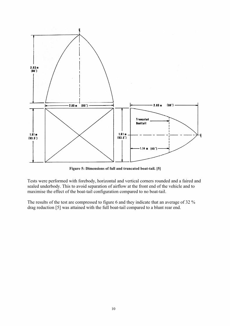
Figure 5: Dimensions of full and truncated boat-tail. [5]

Tests were performed with forebody, horizontal and vertical corners rounded and a faired andsealed underbody. This to avoid separation of airflow at the front end of the vehicle and tomaximise the effect of the boat-tail configuration compared to no boat-tail.

The results of the test are compressed to figure 6 and they indicate that an average of 32 %drag reduction [5] was attained with the full boat-tail compared to a blunt rear end.

10

Figure 6: Aerodynamic drag versus vehicle velocity for different configurations tested at Nasa Dryden. [5]

11

3.1.1. Controlled boundary layers Active separation control system of rear end flow can be performed with tangential blowing assuggested by Englar [6], [7] among others. The technology is also called the Coanda Effectnamed by Henri Coanda. The idea is that a slow airflow that generally would separate over asurface is energized with a high-velocity flow and thus the flow becomes attached to a curvedsurface as shown by figure 7.

Figure 7: The Coanda effect demonstrated on a trailing edge. [6]

This can also be balanced with the possibility to suction of the boundary layer. These twotechnologies combined give the theoretical reduction of 40 % in aerodynamic power.

The trailer configuration simulated at Georgia Tech Research Institute (GTRI) is illustrated infigure 8. The main blowing slots are placed at each rear corners and one slot at the top leadingedge to avoid separation at the front end of the trailer.

Figure 8: The trailer configuration simulated at the Georgia Tech Research Institute. [6]

Blowing all rear slots could reduce spray and drag and just blowing one slot at the rear controlthe aerodynamic side forces and thus give dynamic control to the vehicle. This could forinstance be used to increase lift on the trailer and thus reduce rolling resistance and tire wear.In the opposite way it is possible to increase downforce on the trailer and provide breakingassistance when needed and improve handling during slippery conditions. The effect of windgusts could be controlled and managed with such a system and reduce the risk of jack-knifing.

As a source of airflow GTRI suggested a second turbo generator. This to reduce influence ofengine performance that otherwise would be adverse using bleed of existing turbo pressure orengine exhausts directly.

Using a secondary turbo it is necessary to channel the air from the engine compartment to therear of the trailer. In the case of a standard trailer we assume the length of 7 m for the trailer

12

and the thickness of the walls limit the diameter of the tubes from the extra turbo to the rear ofthe truck to a diameter of approximately 0.1 m. With housing from the extra turbo mounted onthe trucks exhaust system it would give an overall length of the tubing of approximately 10 m.

By assuming airspeed of 30 m/s in the tubes and a friction factor of 0.0015 (fig 7.2 [8]) andusing equation 7.1 from Massey [8] we get a pressure drop of:

Pad

ulfpgdulf

gp

p

l

p

l 3511,0

30100015,02225,12*2

4* 222

=⋅⋅⋅⋅=⋅⋅⋅⋅=∆⇒⋅⋅⋅⋅⋅=

⋅∆ ρρ

(1)

This does not include losses from couplings and bends and similar since the formula is usedfor “long, unobstructed, straight pipes” so the loss can be considered to be even higher. Alower airspeed reduces pressure loss. Another problem using bleeding of turbopressure is thatthe pressure might not be available when breaking and turning since the engine is runningunder low revs and not generating full pressure. A solution might be to add another tank of airunder pressure generated by the compressor to guarantee airsupply under all conditions.

For wind-tunnel tests GTRI used a model described by figure 9.

Figure 9: GTRI wind tunnel model is a generic description of a tractor-trailer configuration. [6]

The GTRI wind-tunnel model has a square section area of 0.83 m2 (1290 sq. in.) and the sizeof the model is a 0.065-scale model of a truck that produced a 5.1 % wind-tunnel blockage.The Reynolds number based on trailer length was 1.9·106 at U = 31 m/s (70 mph) or 3.9·106 attunnel maximum speed.

Figure 10 show the possibility in drag reduction for a 29.5-ton (65 000 pound) 18-wheeltractor-trailer rig with a frontal area of 10 m2 (107.5 sq. ft.).

13

Figure 10: Drag reductions due to blown boundary layers as suggested by GTRI. The upper curvesrepresenting total horsepower required at the wheels to overcome all forces present. [6]

At a speed of 31 m/s (70 mph), power required to overcome drag and rolling resistance can bereduced by 24 respectively 32 % as suggested by Figure 10.

Navier-Stokes equation based Computational Fluid Dynamics analysis was performed atGeorgia Tech School of Aerospace Engineering. Differences in predicted flow are presentedin figures 11a and b.

Figure 11(a-b): CFD predictions of unblown and blown boundary layer performed at Georgia TechSchool of Aerospace Engineering. The reattachment of the flow clearly indicates the possibility to reduce

base-drag of current configuration. [6]

14

GTRI manage to show through wind-tunnel test on the model described above that Cd isreduced by 8 % just by rounding the leading edge of the trailer. If the aft edges are rounded thedrag reduction is of magnitude 7 % and that is without blowing of the boundary layer. Thesesimple steps add up to a drag reduction of 15 % witch clearly is a simple way to reduced fuelconsumption. This is of course when fairing of the tractor-trailer gap is performed. Withoutclosing of the gap between the tractor and the trailer the drag increases dramatically,especially in side-wind conditions.

As figure 12 depicts there can be major gains in blowing the trailing edges of a trailer. Thebenefits of the technology is of course at is best when performed on all four sides. The testswere performed at wind-tunnel speeds of 31 m/s (70 mph), dynamic pressure of 8 Pa (11.86psf) and Reynolds number of 2.51·106 based on total length. At some conditions a 50 % dragreduction was measured when using blown boundary layers.

Figure 12: Drag reduction when blowing different rear trailing edges at tests performed at GTRI. [7]

During some specific conditions, blowing over top and bottom slot only, drag increased. Thiscould be, as mentioned earlier, be useful when breaking the truck.

Some configurations with blown boundary layers and sealed fairing between tractor and trailershow such small values of Cd as some sports cars in the range of 0.3. This is then when the

15

tractor still is missing several ”reality bits” such as engine cooling intake, mirrors, roughunderbody and body component mounting mismatches. When all of these come into play wecan expect Cd to rise to ”normal” values once again. But it is an example of what thetechnology could be able to do in the future when more careful manufacturing methods andattention to details and aerodynamic drag is deployed.

Measurements of lift varied with different slot blowing configurations as can be seen in figure13. These qualities can be used to decrease rolling resistance or increase wheel pressure toreduce breaking distances.

Figure 13: Tests at GTRI show that it is possible to use tangential blowing as a way to increase or decreaselift on the trailer. [7]

P. Ferraresi [9] performed in cooperation with Scania AB a series of CFD tests based on asimple truck model consisting of a prism with rounded edges and without wheels. Comparisonwas made with a wind-tunnel model based on the Peps configuration with the Volvo wind-tunnel as reference. The Peps configuration is an aerodynamical ideal truck-trailercombination with 5.3 m length, 1.3 m width and 2 m height.

16

At a simulated velocity of 44.4 m/s and a reference frontal area of 1.3 m2, only half of thetruck was modelled due to symmetry reasons, the results suggests a 29 % reduction in dragwithout blowing the boundary layers as table 2 show and the different configurations tested isshown in figure 14.

Truck configuration Cd ReductionBasic 0.326

Boat-tail, lt = 0.5,ϕ = 15° 0.23 29 %Boat-tail, lt = 0.25,ϕ = 15° 0.271 17 %Boat-tail, lt = 0.1,ϕ = 15° 0.285 12 %

Round, radius = 0.1 m 0.293 10 %Round, radius = 0.2 m 0.28 14 %

Table 1: Result for CFD calculations at KTH. Reductions in drag are clear and this is without blowing ofthe boundary layers where lt = tail length [m] and ϕ =tail angle. [9]

Figure 14: Different configurations simulated at KTH. [9]

Figure 15 present a reduction in drag for the rounded section as the radius increase.

Figure 15: Cd versus rear end rounding radius. [9]

17

Further simulations were done with blowing of the boundary layer. The results are presentedin table 2 and suggest a drag reduction of 29 % for boat-tail configuration and 17 % dragreduction for a rounded rear end configuration.

Configuration Cd

Basic 0.326Boat-tail Length = 0.1 m Basic 0.285

Blowing 0.287, U = 0.4 m/s0.275, U = 0.004 m/s

Length = 0.25 m Basic 0.271Blowing 0.291, U = 2 m/s

0.338, U = 33 m/sLength = 0.5 m Basic 0.23

Blowing 0.25, U = 0.4 m/sRound Radius = 0.1 m Basic 0.293

Blowing upper 0.278, U = 0.04 m/s Blowing upper +lateral

0.27, U = 0.04 m/s

Punctual Blowing 0.28, U = 0.04 m/sRadius = 0.2 m Basic 0.28

Blowing 0.27, U = 0.04 m/sTable 2: Result for CFD calculations at KTH when blowing the boundary layers. [9]

As before a long boat-tail proves to be the best configuration but the most interesting fact isthat drag increase when blowing the boundary layer for that configuration. Suction was alsotested and the results are presented in table 3 with a decrease of Cd of 29 % for boat-tail withlength of 0.5 m and 24 % for a rear radius of 0.1 m.

Configuration Cd

Basic 0.326Boat-tail Length = 0.1 m Basic 0.285

Suction 0.283Length = 0.25 m Basic 0.271

Suction 0.27Length = 0.5 m Basic 0.23

Suction 0.23Round Radius = 0.1 m Basic 0.293

Suction upper 0.27, U = 0.04 m/s Suction upper +lateral

0.247, P = -2500 PaAverage

Points 0.27, P = -2500 PaRadius = 0.2 m Basic 0.28

Suction upper 0.27, U = 0.04 m/s0.265, P = -2200 Pa

Table 3: Result for CFD calculations at KTH when suction is applied to the boundary layer. [9]

The effects on the boat-tail (compared to no blowing or suction) is as before very small andwill probably be balanced out by the energy required to propel any device for suction orblowing of the boundary layer. For the rounded trailing edges blowing and suction provide a

18

clear difference in performance. Since rounding of the edges is more beneficial consideringspacing for passengers and load (cargo) it might be interesting to further investigate thistechnique.

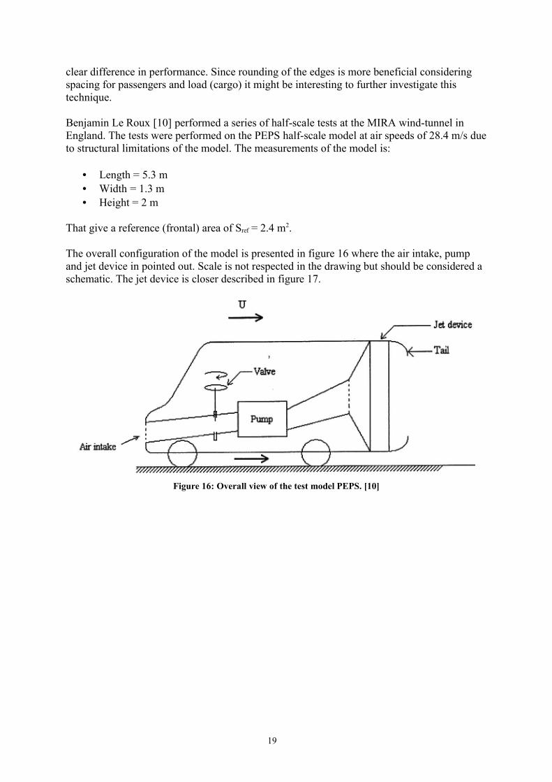
Benjamin Le Roux [10] performed a series of half-scale tests at the MIRA wind-tunnel inEngland. The tests were performed on the PEPS half-scale model at air speeds of 28.4 m/s dueto structural limitations of the model. The measurements of the model is:

• Length = 5.3 m• Width = 1.3 m• Height = 2 m

That give a reference (frontal) area of Sref = 2.4 m2.

The overall configuration of the model is presented in figure 16 where the air intake, pumpand jet device in pointed out. Scale is not respected in the drawing but should be considered aschematic. The jet device is closer described in figure 17.

Figure 16: Overall view of the test model PEPS. [10]

19

Figure 17: Jet device’s section with a tail and pressure taps. [10]

The jet device cover the circumference of the aft of the truck and the air outlet is just belowthe “S” in figure 17. This gives the tangential blowing that is investigated. In order to maintaina steady flow the volume before the outlet is large and work as a plenum to equal outdifferences in pressure.

The tail section is defined by figure 18 and their variations during the tests are accounted forin table 4.

Figur 18: Tail section. L1- Flat extension of the trailer to study the effect of the location of the jet from theturning surface. R- Radius of the rounded part. α- Angle of the rounded part. L2- Flat part as a boat-tail.

[10]

20

Table 4: Variations of tail parameters during the MIRA tests. [10]

The length and height of the tail is given by formulas 2 and 3)cos()sin( 21 αα ⋅+⋅+= LRLLtail (2))sin())cos(1( 2 αα ⋅+−⋅= LRH tail (3)

The first aim of the experiments was to determine the best tail configurations. This was doneusing a 3 mm slot with blown and non-blown boundary layers to determine whichconfiguration was most beneficial. Figure 18 show the different configurations tested andtable 5 present the results.

21

Figure 19: Different tail configurations tested at the MIRA wind-tunnel. [10]

Name Description Cd without

blowing

Cd withmaximum

blowing

∆Cd [points](positive for

decreasing drag)Baseline 0,344 0,348 -4

T2 Rounded 0,347 0,338 9T3 Rounded 0,346 0,339 7T4 Rounded 0,340 0,340 0T5 Rounded 0,341 0,332 9T6 Mixed 0,345 0,346 -1T7 Boat-tail 0,312 0,301 11T8 Boat-tail 0,340 0,314 26T9 Boat-tail 0,357 0,365 -8TI0 Mixed 0,359 0,348 11T11 Mixed 0,344 0,342 2T 12 Mixed 0,343 0,347 -4T13 Mixed 0,347 0,350 -3T 14 Mixed 0,345 0,352 -7

Table 5: Test results from MIRA with and without blowing of the boundary layers. [10]

22

It is clearly seen that configurations 7 and 8 are those who present the lowest drag and largestdifference in Cd. Comparison between the tails 3, 11 and 12 shows that increased length of L1

is not beneficial for drag reduction.

Tail number 5 show that there is no point in extending the tail beyond the point of separation,on the contrary, a prolonged tail beyond that point increase drag. So it would be interesting tofind the point of separation and thus optimise tail length. But all these values are lowcompared to the ones achieved when using boat-tails and that configuration is to prefer.

The most beneficial configuration would be the 15° tail as confirmed by other tests at othertimes and as is shown by table 5. Further investigation of tail 8 was done since it in an earlystage showed the highest drag drop. Different blow ratios and slot heights were tested and theslot height of 1 mm seems to be the most efficient. This might not directly be transferred to afull-scale model so in that case optimal slot height must be found.

The power savings on this devise was about 20 % compared to the reference values and wasachieved as earlier mentioned with tail 8 and maximum blowing.

3.1.2. Aerodynamic boat-tailAn aerodynamic boat-tail, also called boat-tail plates, was evaluated at Nasa Ames ResearchCentre [11]. The configuration is described by figure 20. The idea is to trap a vortex or eddyin the corner between the rear of the trailer and boat-tail plates. The dimensions of the truck isnot given in the report [11] but is assumed to be of standard dimensions.

Figure 20: The configuration of aerodynamic boat-tail compared to ordinary rigid boat-tail. [11]

The eddy turn the flow inwards as it separates from the rear of the trailer and creates a virtualboat-tail and thus increase the base pressure acting on the rear of the vehicle and reduce the

23

net aerodynamic drag of the vehicle. Figure 21 show the aerodynamic boat-tail mounted onthe rear end of the truck.

Figure 21: The rear end configuration of the trailer when performed wind-tunnel tests according toLanser et. al. at the Nasa Ames Research Centre. [11]

Table 6 show the different geometrical configurations tested.

LP DV Dh

0.0 0,0 0,00.24 0.04 0,04

0,24 0.06 0.06

0.24 0.12 0.120.30 0.04 0,040.30 0,06 0.06

0.30 0,09 0.09

0.30 0.04 0.060,30 0.06 0.090.36 0.04 0,04

0.36 0,06 0,06

0.36 0.12 0.12 0.36 0.15 0.150.36 0.04 0,060.44 0.04 0.04

0.44 0.06 0.060.44 0.09 0.09

Table 6: Different configurations tested at the Nasa Ames Research Centre using the aerodynamic boat-tail described in Figure 21. All lengths and distances are normalised by the trailer width. [11]

24

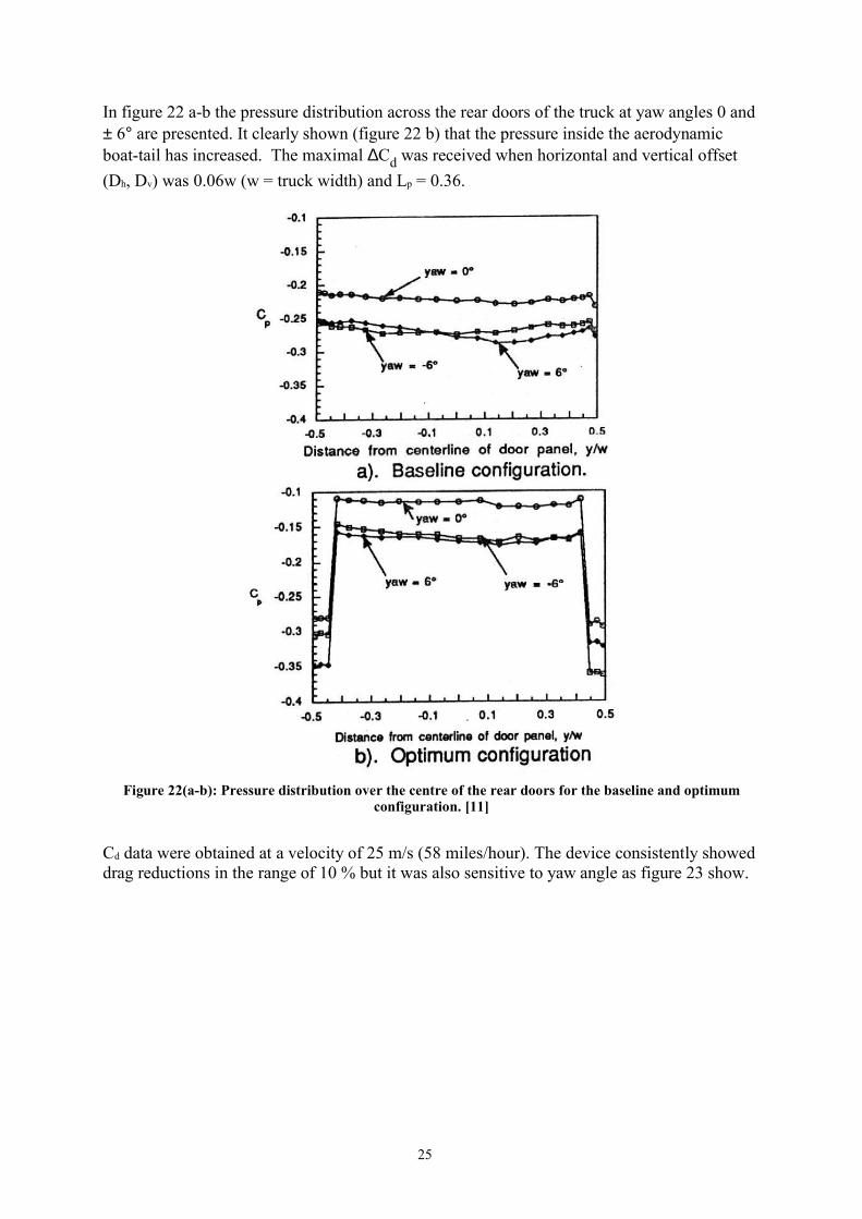
In figure 22 a-b the pressure distribution across the rear doors of the truck at yaw angles 0 and± 6° are presented. It clearly shown (figure 22 b) that the pressure inside the aerodynamicboat-tail has increased. The maximal ∆Cd was received when horizontal and vertical offset(Dh, Dv) was 0.06w (w = truck width) and Lp = 0.36.

Figure 22(a-b): Pressure distribution over the centre of the rear doors for the baseline and optimumconfiguration. [11]

Cd data were obtained at a velocity of 25 m/s (58 miles/hour). The device consistently showeddrag reductions in the range of 10 % but it was also sensitive to yaw angle as figure 23 show.

25

Figure 23: Change in drag as a function of yaw angle when optimum aerodynamic boat-tail is mounted.CD,ref is the original Cd of the truck with no aerodynamic devise mounted at the rear. [11]

26

3.2.GroovesAnother technology developed by J.C. Lin et. al. [12] but originating in the Soviet Union isthe use of transverse and swept grooves. The work was performed on a diffuser but should beapplicable on other areas too. Some 50 % drag reduction has been reported on bluff bodieswith grooves.

J.C. Lin et. al. performed their tests at a Reynolds number of 5.1·106 at NASA Langley 51 x71 cm tunnel, that is a low-turbulence, subsonic, open-circuit tunnel. Tests were performed atfree-stream velocity of 40.2 m/s. Figure 24 describes the test configuration used. A suctionslot was installed in front of the test section to remove any upstream influence on the testsection. The ceiling of the tunnel above the test section was adjusted in a way to ensure a zeropressure gradient.

Figure 24: The test configuration at NASA Langley wind-tunnel performing test of grooves over abackward-facing ramp. [12]

The boundary layer just ahead of the separation ramp was fully turbulent and approximately3.25 cm in thickness. The shoulder radius of the ramp was 20.3 cm (8 in.) and the ramp was ata 25º as shown by figure 24. The width of the test section was to full wind-tunnel width of 71cm.

The flow separated at approximately the midpoint of the ramp without the grooves. Thegrooves were placed on the shoulder of the ramp and different geometries tested are presentedin figure 25.

27

3.2.1. Transverse and swept grooves

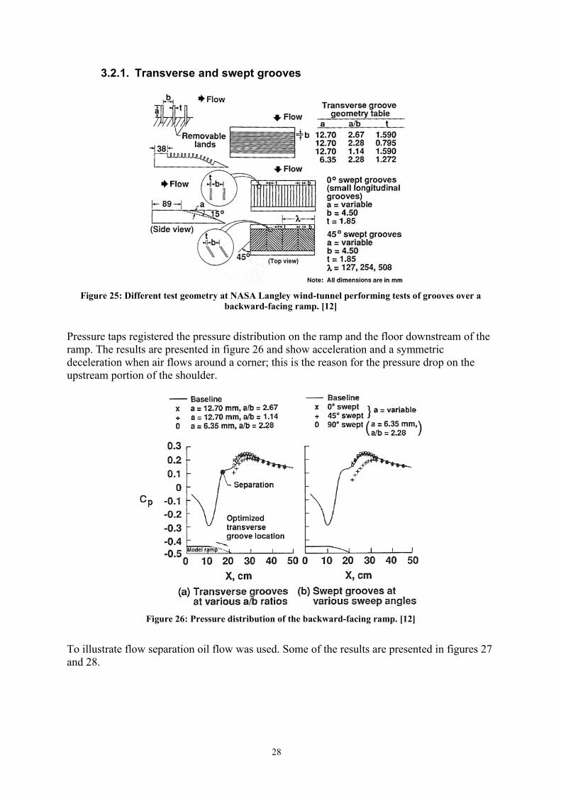
Figure 25: Different test geometry at NASA Langley wind-tunnel performing tests of grooves over abackward-facing ramp. [12]

Pressure taps registered the pressure distribution on the ramp and the floor downstream of theramp. The results are presented in figure 26 and show acceleration and a symmetricdeceleration when air flows around a corner; this is the reason for the pressure drop on theupstream portion of the shoulder.

Figure 26: Pressure distribution of the backward-facing ramp. [12]

To illustrate flow separation oil flow was used. Some of the results are presented in figures 27and 28.

28

Figure 27: Oil flow over different ramp models were a) is the reference model and b) the model withtransverse grooves. [12]

Figure 28: Oil flow over different ramp models where a) has longitudinal grooves and b) have 45 degreeswept grooves. [12]

An optimum placement for transverse grooves proved to be to begin with the grooves oneboundary-layer thickness upstream of the base model separation line and extending oneboundary-layer thickness downstream of the separation line. This configuration reduced thedistance from separation to reattachment by 20 %. The most effective configuration proved tohave a depth-to-width ratio (a/b) of 2.67. Reduction of depth-to-width ratio reducedeffectiveness of the device.

29

Using longitudinal and 45 degree swept grooves the depth (a) varied along each groove, fromzero depth at the leading edge to about 0.64 cm at the midpoint. Since the pressure recovery(figure 26) is not as large using 45-degree grooves as using transverse we have an adverseresult using the 45-degree grooves compared to baseline configuration. This could beexplained by the same phenomenon as for transverse groves with depth-to-width ratio of 1.14;the distance between the grooves is too small and the airflow experiences it as a closed cavityand thus there is no reduction in reattachment distance (the distance from reference separationline to maximum pressure coefficient).

The mechanism associated with different improvements in pressure recovery and reduction inreattachment distance is for the transverse grooves a “roller bearing” mechanism that can beexplained in such way that the air rolls or rotates in each individual groove. For thelongitudinal grooves it could be the technique of partial “boat-tailing”.

J. C. Lin et al [13] performed another series of tests that included many more differentmethods to improve pressure recovery on a backward facing ramp. The tests performed atNASA Langley [13] were performed at the same tunnel and same configuration as the testswith grooves described above [12]. The different test configurations are illustrated by figure29 a-d.

30

Figure 29 (a-d): Geometry of separation control devices. [13]

31

In contrary to what is said before [12] it is now stated [13] that a correct design of sweptgrooves probably will be more efficient than transversal grooves. That is founded on fact thatthere is a three-dimensional flow generated by the transversal grooves that is shown in figure27 and this is what generate the beneficial flow. A proper design of swept grooves wouldreinforce this behaviour and possibly generate a reduction in reattachment distance.

Optimum transverse configuration described by figure 30, where a/b = 2.67, reduced thedistance to reattachment by almost 50 %.

Figure 30: Pressure distributions for transverse grooves. [13]

3.2.2. Longitudinal groovesFigure 29 c show the different longitudinal grooves that were tested. Figures 31 show thepressure distribution using the different grooves.

Figure 31: Pressure distribution for longitudinal grooves with 2-inch spacing. [13]

A separation of 50,8 mm (2 inches) between each groove proved to be most efficient spacingthat were tested; it significantly reduced the distance to reattachment. As figure 31 show the

32

short V-grooves proved to be the most efficient configuration under these tests and it reducedthe reattachment distance by 66 %. Worth mentioning can be that ‘short’-, ‘long’- and sine-wave grooves had a shorter reattachment distance than the smaller zero-sweep anglelongitudinal grooves mentioned earlier [12]. For a 100 mm (4 inch) distance between thegrooves the sine-wave configuration proved to be more efficient.

3.2.3. Passive porous surfaceThis technology has its background in drag reduction on trans- and super-sonic wings. Dragreduction is achieved by placing a thin cavity with porous surface where the shock wave islocated. The higher pressure behind the shockwave circulates the air through the cavity to thelower pressure ahead of the shock. This effects both boundary-layer separation and entropy ina positive way.

The techniques tested are described in figure 29 b. A fully porous surface has little or nopositive effect on the pressure distribution. But a non-porous surface separating a poroussurface downstream and tangential blowing slot upstream has some positive on pressuredistribution as illustrated by figure 32.

Figure 32: Pressure distribution for passive tangential blowing. [13]

The most beneficial configuration is when the 0.8 mm (0.032-inch) tangential gap is placed atthe baseline separation location (location C in figure 32). The problems with the technique(pressure driven self-bleeding) are probably due to insufficient mass flow but the technologymight have applications for more severely separated cases with larger adverse pressuregradients.

33

3.3.Vortex generatorsVortex generators have normally been used to increase low speed, high angle performance onaircraft and to reattach separated flow on airfoils. On a flap deflection of 35° Lin et. al. [14]managed to reattach the airflow completely.

Wheeler vortex generators have in commercial tests within the trucking industry [13]indicated up to 10 % fuel mileage improvement.

When performing tests at the NASA Langley wind tunnel [13], to be able to measure the dragof the vortex generators a balance was used. A Piezoresistive deflection sensor was used toconvert displacement into drag force. The range of the balance was 0 – 8.9 kPa (0 – 1.3 lbf)with a resolution of 1.5 Pa (2.2·10-4 lbf.) The measurement of the drag was conducted withvortex generators placed 152 mm (6 inches) and 1067 mm (42 inches) upstream of theseparation ramp described in figure 24.

3.3.1. Vane-type vortex generatorsOne-inch-high vane-type counter rotating vortex generators as described by figure 29 d wasinitially tested and it provided attached flow directly downstream the generators. When movedfrom 5δ (16 cm) to 15δ (49 cm) upstream of the baseline separation line the generatorsmaintained their efficiency. Figure 33 show three spanwise pressure distributions at 0, λ/4 andλ/2 distance away from the device centreline.

Figure 33: Pressure distribution for 1-inch-high counter-rotating vortex generators at 5d upstream of thebaseline separation. [13]

Figure 33 also show an improved pressure recovery but also a reduction of pressure on rampsshoulder region. This is desirable if one wants to increase lift but result in a pressure dragpenalty. The reduction in pressure is caused by increase in local velocity resulting from theredirection of high momentum airflow from outer parts of boundary layer.

34

3.3.2. Wheeler vortex generatorsThe configuration with Wheeler generators is illustrated by figure 29 d.

Flow visualisations for the Wheeler vortex generators show that the optimal placement is justahead of the horizontal tangential location on the shoulder of the separation ramp. Oil flowvisualisations indicate that both 12,5- and 3- mm (½- and 1/8- inch) high generators, whenplaced at the optimum location, are efficient and reduce reattachment distance up to 66 %.

Figure 34 a and b show pressure distributions for different spanwise location of pressure taps.Figure 34 a for the 12,5 mm high generators and figure 34 b for the 3 mm high generators.The variations are much smaller than for the vane-type generators and the 3 mm Wheelergenerators produce virtually no difference in pressure distribution spanwise.

Figure 34(a-b): Pressure distributions for Wheeler vortex generators. [13]

35

Since the Wheeler vortex generators produce less three-dimensional flow, indicated by thelack of variation in pressure distribution spanwise, it minimise pressure reduction at theshoulder of the ramp and thus is more beneficial for pressure-drag reduction.

The beneficial behaviour of the low Wheeler generators is because the turbulent velocityprofile of the boundary layer as described by figure 35.

Figure 35: Location height to boundary layer profile. [13]

At device heights of 0.2 δ the local velocity is over 75 % of the free-stream value and furtherincrease in height only give minor addition to air speed.

J.C. Lin summarised the results [15] in figure 36 and illustrate the baseline configurationseparation compared to the configurations with VG using oilflow as shown in figure 37 a-c.

36

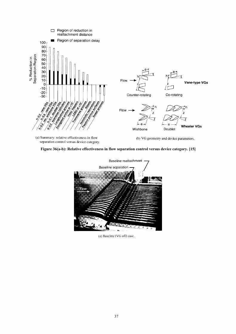
Figure 36(a-b): Relative effectiveness in flow separation control versus device category. [15]

37

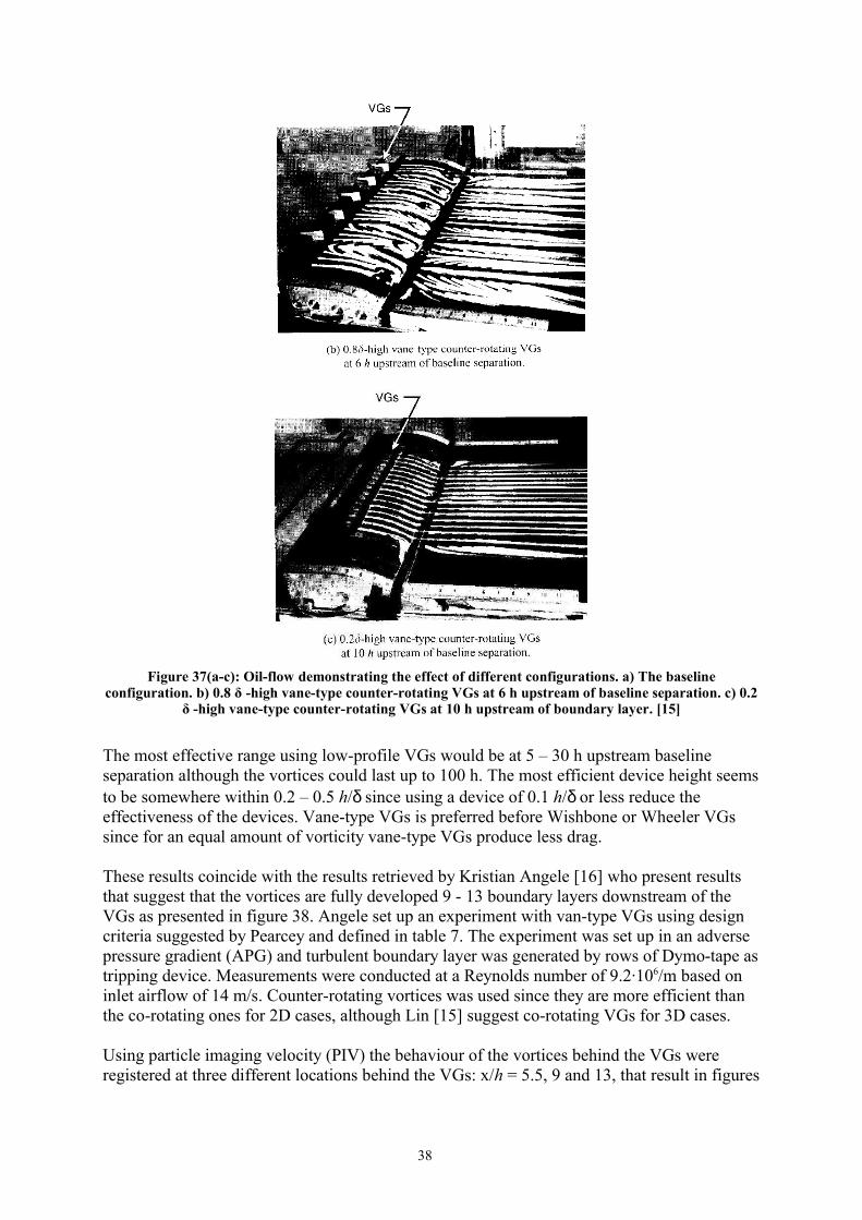
Figure 37(a-c): Oil-flow demonstrating the effect of different configurations. a) The baselineconfiguration. b) 0.8 δ -high vane-type counter-rotating VGs at 6 h upstream of baseline separation. c) 0.2

δ -high vane-type counter-rotating VGs at 10 h upstream of boundary layer. [15]

The most effective range using low-profile VGs would be at 5 – 30 h upstream baselineseparation although the vortices could last up to 100 h. The most efficient device height seemsto be somewhere within 0.2 – 0.5 h/δ since using a device of 0.1 h/δ or less reduce theeffectiveness of the devices. Vane-type VGs is preferred before Wishbone or Wheeler VGssince for an equal amount of vorticity vane-type VGs produce less drag.

These results coincide with the results retrieved by Kristian Angele [16] who present resultsthat suggest that the vortices are fully developed 9 - 13 boundary layers downstream of theVGs as presented in figure 38. Angele set up an experiment with van-type VGs using designcriteria suggested by Pearcey and defined in table 7. The experiment was set up in an adversepressure gradient (APG) and turbulent boundary layer was generated by rows of Dymo-tape astripping device. Measurements were conducted at a Reynolds number of 9.2·106/m based oninlet airflow of 14 m/s. Counter-rotating vortices was used since they are more efficient thanthe co-rotating ones for 2D cases, although Lin [15] suggest co-rotating VGs for 3D cases.

Using particle imaging velocity (PIV) the behaviour of the vortices behind the VGs wereregistered at three different locations behind the VGs: x/h = 5.5, 9 and 13, that result in figures

38

38 a-f. They confirm the statements that a fully energized boundary layer takes some 15boundary layers downstream the VGs to fully develop.

Figure 38(a-f): Secondary flow components generated by VGs in the yz-plane (perpendicular to thegeneral airflow direction). a-b) x/h = 5.5 c-d) x/h = 9 e-f) x/h = 13. v2 and w2 are the different crossflow

components in the yz-plane. [16]

l h d δ β30 mm 10 mm 25 mm 10 mm 15°

Table 7: Definition of experimental set up by K. Angele. [16]

Low-profile VGs probably need a further distance to develop since they interact with a smallerpart of the boundary layer than the boundary layer sized VGs used in the K. Angeleexperiments.

39

Another successful attempt to use low-profile VGs is presented on the flow over a backwardfacing ramp dominated by a 3D separated flow generated by two large junction vortices – oneover each side-corner of the ramp. Figure 39 a show the large spiral nodes at the ramps sideedges and the reverse flow at the centre of the ramp.

Figure 39(a-b): Oil flow visualizations on the effect of using VGs to reduce 3D flow over a backward-facing ramp. [15]

Figure 39 b show how low-profile VGs (h/δ = 0.2, e/h = 4, ∆z/h=4, β= 23°, airspeed 42.7 m/s(140 ft/s)) efficiently reduce the flow separation and the flow in the centre of the ramp

40

maintain attached. Further investigation also suggests that there is no major difference ineffectiveness of the low-profile VGs when placed somewhere 20 h upstream of baselineconfiguration separation.

3.3.3. Blunt body application of Vortex GeneratorsW. Calarese et. al. [17] performed a series of experiments on the effect of vortex generatorson total drag of a 1/72 scale model of a C-130 aircraft. The model was selected because of its highly up-swept afterbody that generate a high adverse pressure gradient and the wish from itsoperators (US Airforce) to reduce its fuel consumption.

Tests were performed at Air Force Institute of Technology. Their wind tunnel is an openreturn, closed section tunnel with a circular test section of 1.524 m (5 ft.) in diameter and5.4864 m (18 ft.) in length. The balance is a 3-component wire balance with accuracy within0.0002 N (0.02 pound.), 40 pressure taps were placed at the bottom and side of the rearfuselage and on the up-swept afterbody. For placement see figure 40.

Figure 40: Schematic of pressure taps. [17]

Boundary layer thickness that was defined by the formula of a flat plate in turbulent flow asdefined by equation 4.

( ) 51

Re

37.0 Tx⋅=δ (4)

The turbulent boundary layer begun at the tripwire illustrated in figure 40 and the distance tothe up-sweep line from this location was xT = 190 mm (7.5 inch.) A Reynolds number of5.78·105 resulted in a boundary layer thickness of δ = 4.8 mm (0.19 inch.).

41

The tests were performed at a Mach number of 0.135 (45 m/s) or a dynamic pressure of 89.3Pa (60 psf.). All tests were repeated and the data agreed within ± 2 %. The net drag coefficientfor the C-130 was measured to a Cd of 0.05 at α = 0°. This was consistent with previous datafor that model of aircraft.

The two placements of the vortex generators used in tests were 10 δ upstream of the afterbodyup-sweep line and 4 δ upstream the same line as defined in figure 41 with an angle of 16°towards the freestream flow circumferentially around the fuselage. The vortex generators cordwas 10.2 mm (0.4 inch) and their span (= device height) was 1.1 times the boundary layerthickness. The trailing edges of the VG were spaced with a distance of 15.2 mm (0.6 inch) asillustrated by figure 41.

Figure 41: Vortex generators alignment and dimensions. [17]

Another series of tests was performed using small flat stubs with a cord of 1.3 mm (0.05inch), a span of 4.2 mm (0.165 inch) and a thickness of 0.3 mm (0.012 inch) as defined infigure 41 with an angle of 16° towards the freestream flow. 16 to 22 pairs were usedcircumferentially around the fuselage and the distance between them were 5 mm (0.2 inch).The “forward” location was 8 δ (38 mm) upstream the afterbody up-sweep line and the “aft”location approximately 4 δ (19 mm) upstream the same line as defined in figure 41.

42

The usage of VG resulted in a reduction of the drag coefficient of about 150 counts asdemonstrated by figure 42.

Figure 42: Total drag variation with angle of attack. [17]

But the result for the ”stubs” is even better: a reduction of 300 counts is obtained as is shownin figure 43.

Figure 43: Total drag variation with angle of attack. [17]

43

The reduction in drag is more efficient at lower angles of attach and this is beneficial sincethis correspond to cruise conditions and this is the condition the aircraft operates at the mostof the time. The placement of both the VG and the stubs in the “front” location generated thebiggest reductions in drag coefficient. This can be explained by the fact that placement of theVG and stubs on the forward location give the airflow enough time to mix with the freestreamflow and thus energize the boundary layer flow, delaying the separation at the up-sweep line.

These results are all in line with those achieved by J.C. Lin et. al. [15] and show the potentialof using sub-boundary layer vortex generators in reducing bluff body drag. The smaller deviceheights give a smaller device drag but give enough energizing of the boundary layer ifcarefully placed.

Based on the results in [15] and [16] it easy to belief that it is beneficial to place VGs as farupstream as possible. But Lin [15] also shows that placement to far upstream can increaseflow separation and drag. The Naval Surface Warfare Centre performed some CFDcalculations on the overwing fairing of a V-22 aircraft simulating ten low-profile VGs. Figure44 a illustrate a cruise angel of 7° and light separation. In figure 44 b the placement too farupstream (or too large VGs) of the VGs generate increased separation. By moving thegenerators 10 device heights downstream the baseline separation (figure 44 c) is eliminated.

44

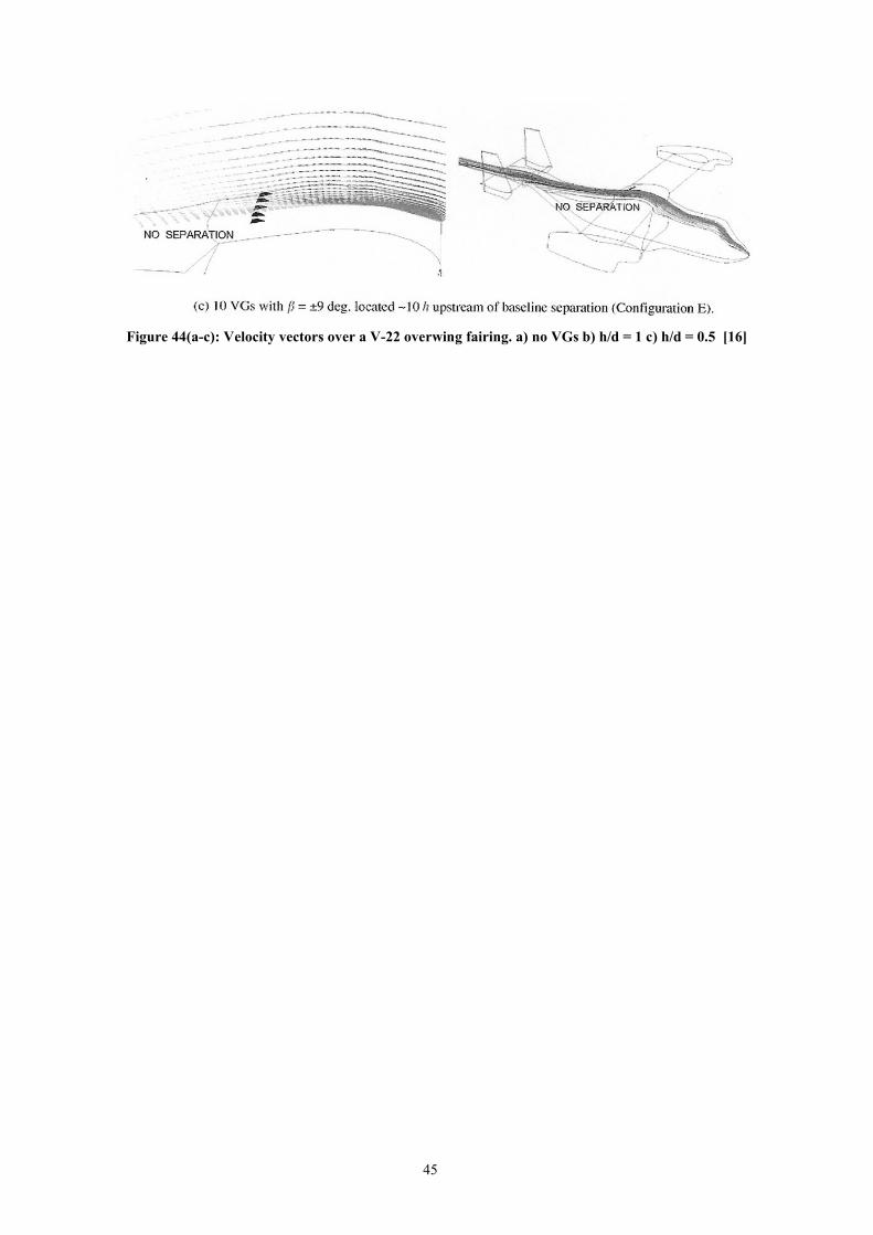
Figure 44(a-c): Velocity vectors over a V-22 overwing fairing. a) no VGs b) h/d = 1 c) h/d = 0.5 [16]

45

4. Continued workFurther investigations has been done in the areas of boundary layer control but has not beenaccounted for in this report. An alternative approach that could be used is the use of soundwaves to control the boundary layer separation as suggested by A. Nishizawa and S. Takagi[18].

One of the most interesting areas would be the use of air jets to form vortex generators assuggested by H. Abe et. al. [19]. The benefit with that technology is that it would be possibleto control the strength of the jets and thus control the strength of the vortices created. Thiscould translate into different grade of flow attachment at different flow situations and mostbeneficial of all is the possibility to shut them down and in that case they do not in any waycontribute to the overall drag. The downside of them is the same as for controlling boundarylayer with blowing and suction; it requires additional equipment for generating the airflowsand some kind of control mechanism. That adds cost and complexity to the construction andthat is never a good thing in terms of maintenance and cost.

46

5. ConclusionsMentionable is that there are measures that are more important to take than changing theairflow around the rear of a vehicle. Those measures are the rounding of front corners whichcan contribute to as much as 52% drag reduction [6] and a full-length underbody seal cancontribute to as much as 15% drag reduction [6]. These measures needs to be taken care ofbefore it is interesting to take a look at rear end flow. But when at least the first measure hasbeen taken care of it can be beneficial to take a look at altering rear end airflow.

Based on the results given in [13] and [15] I belief that the most efficient way to reduce base-drag on blunt bodies (such as busses and trucks) is the use of VGs in some way. Preferablylow-profile ones to reduce device drag or air-jet VGs that can be turned on and of duringdifferent conditions.

One conclusion that can be made from the different reports referred to in this work is that it isdifficult to receive the same result in wind-tunnel tests as those received in simulations. Thisis of course explained by the fact that there are “reality-factors” included in the resultsreceived from wind-tunnel tests. That is imperfections in manufacturing of the model, leakageand general losses that is not accounted for in CFD modelling.

Some of the results are gathered in table 8.

Technology Type of improvementBoat-tailing 32 % reduction in Cd.Aerodynamic boat-tail 10 % reduction in Cd.Blown boundary layers at GTRI 50 % reduction in Cd. *CFD, round rear edge 14 % reduction in Cd.CFD, round rear edge, suction of bl** 24 % reduction in Cd.Wind-tunnel test, boat-tail, blowing of bl** 12 % reduction in Cd.Transversal grooves on a shoulder 20 % shorter distance to reattachmentLongitudinal grooves on a shoulder 66 % shorter distance to reattachmentAngled grooves on a shoulder Not conclusive ***Passive porous surface Some improvementMicro vortex generators 300 counts

Table 8: Summary of some of the results presented in the report. *=compared to no aerodynamicoptimisation at all = sharp front end, no fairing. **bl=boundary layer. ***= [12] suggest a 50 % drag

reduction

Judging from these results it seems like blowing boundary layers would be the most beneficialway to reduce rear end drag. But in this case, and several others, there is the “reality factor” toconsider as mentioned above in this section, tests performed at GTRI was performed on an“ideal body” and can not be easily be compared to other results.

Then there is the traditional boat-tailing that come in second. These results are more reliablesince they are performed on a real vehicle, still it is ideal in many ways but they give a hint ofwhat kind of results we want to achieve. And as I mentioned earlier they can be used as abench mark for other tests since they present the most ideal flow case (a full boat-tail) butwith some separation so that result can be somewhat improved. Results much better than this(for example the GTRI result) should be seen upon with some scepticism before presented toothers. Or at least thoroughly explained why that kind of result is received.

47

So in real life, what seems to be the best technology to apply to your vehicles? With little orno difference in manufacturing technology rounding of the rear edges seems so far to be thebest way as for now to receive smaller contribution to the overall drag. In combination withgrooves could improve the pressure recovery mechanism at the rear of blunt vehicles and withproper placement and design I belief that VGs in some kind belong to future design of highperforming commercial vehicles.

48

6. References[1] Wolf-Heinrich Hucho; Aerodynamics of Road Vehicles, ISBN 0-7680-0029-7[2] Alfons Gilhaus; The main parameters determining the aerodynamic drag of buses, NeueTechnologie, M.A.N. München, June 1981 [3] Edwin J. Saltzman; A summary of NASA Dryden’s Truck Aerodynamic Research, SAETechnical Paper Series, 821284[4] Robert D. Blevins; Applied fluid dynamics handbook, ISBN 0-442-21296-8[5] Randall L. Peterson; Drag reduction by the addition of a boat-tail to a box shaped vehicle,NASA Contractor Report 163113, August 1981[6] Robert J. Englar; Development of Pneumatic Aerodynamic Devices to Improve thePerformance, Economics, and Safety of Heavy Vehicles. SAE Paper 2000-01-2208. June 19-21, 2000[7] Robert J. Englar; Advanced Aerodynamic Devices to Improve the Performance,Economics, Handling and Safety of Heavy Vehicles. SAE Paper 2001-01-2072. May 14-16,2001[8] B.S. Massey, Mechanics of Fluids, sixth edition, ISBN 0-412-34-280-4[9] Paola Ferraresi; Control of Boundary Layer Flow on Trucks. Master Thesis, Skrift 2001-14. Department of Aeronautics, Royal Institute of Technology, SE-100 44 Stockholm, Sweden[10] Benjamin Le Roux; Experimental Aerodynamics: Separation Control on Trailers ofTrucks, A Master Thesis at Scania CV AB, RTTF section. May 2003[11] Wendy R. Lanser, James C. Ross and Andrew E. Kaufman; Aerodynamic Performance ofa Drag Reduction Device on a Full-Scale Tractor/Trailer, SAE Paper912125[12] G.V. Selby, J.C. Lin and F.G. Howard. Turbulent flow separation control over abackward-facing ramp via transverse and swept grooves. Journal of Fluids Engineering, June1990, Vol. 112[13] J. C. Lin and F. G. Howard, Turbulent Flow Separation Control Through PassiveTechniques. NASA Langley Research Research Center, Hampton, VA; and G.V. Selby, OldDominion University, Norfolk, VA. AIAA 89-0976. March 13-16, 1989[14] S. Klausmeyer, M. Papadakis, J. Lin; A Flow Phisics Study of Vortex Generators on aMulti-Element Airfoil, AIAA 96-0548[15] John C. Lin; Review of research on low-profile vortex generators to control boundary-layer separation. Progress in Aerospace Sciences 38 (2002) 389-420. [16] Kristian Angele; Experimental studies of turbulent boundary layer separation and control.Royal Institute of Technology, Department of Mechanics. Technical report 2003:08. ISSN0348-467X[17] W. Calarese, W.P. Crisler and G.L. Gustafson; Afterbody Drag Reduction by VortexGenerators, Flight Dynamics Laboratory, Air Force Wright Aeronautical Laboratories,Wright_Patterson Air Force base, Ohio. AIAA-85-0354. January 14-17, 1985/ Reno, Nevada[18] Akira Nishizawa, Shohei Takagi; Toward smart control of separation around a wing –Development of an Active Separation Control System, National Aerospace Laboratory ofJapan, Chofu, Tokyo, 182-8522[19] Hiroyuki Abe, Takehiko Segawa, Takayuki Matsunuma, Hiro Yoshida; Management of aLongitudinal Vortex for Separation Control, National Institute of Advanced Industrial Scienceand Technology, Japan

49