11/11/2017

1

Alonso G Griborio, PhD, PE1

Randal W Samstag, MS, PE, BCEE2

1 Hazen and Sawyer, Hollywood, FL, US2 Civil and Sanitary Engineer, Bainbridge Island, WA, US

• Introduction• Clarifier Modeling Options• Role of Models• Calibration and Verification Definitions

• 2-D and 3-D Modeling• General Modeling Process• Model Calibration

• 2-D Case Study• 2Dc Model

• 3-D Case Study• Square Clarifier Field Test and CFD• Radial clarifier EDI Evaluation Case Histories

11/11/2017

2

ClarifierM odelingO ptions

Box models

1-D models

2-D models

3-D models

Effective use of all levels of models

Increasing rigor

SOR

Vs

SOR+UFR

Xj

j+1jj-1

UFR

1-D Model

Level Strength Application Weakness

Hazen S im ple Discretesettling(Grit) Ignoreshydrodynam ics

L im itS tate

S im ple Zonesettling(S S T prelim inary designandoperational)

Ignoreshydrodynam ics

1D Com putationspeed A lltypesofsettlingincluding2 phaseflow s

Ignoreshydrodynam ics

2D Com putationspeedcom paredto3D;runsonlaptop.

A llclarifiersw herethereisadom inantflowdirection;dynam icsim ulations.

Ignoreslateralnon-uniform ity insolidsandm om entum .

3D Com pletenessofgoverningequations;highspatialresolution.

A llclarifiers.S teady statesim ulationsw hereadom inantflow directioncannotbeassum ed.

L ongexecutiontim es;highlevelofexpertiserequired.

McCorquodale et al. WWTmod 2010 Presentation

11/11/2017

3

•Calibration: Initial trials toadjust model parameters toreproduce field conditions(either long term data orfield testing data).

•Verification/Validation:Tests to confirm that a modelis representing fieldconditions. For example byindependent stress testswith different flow or settlingconditions or operating data

11/11/2017

4

Wicklein et al. (2016) “Good modelling practice in applying computational fluid dynamics for WWTP modelling” WST 73.5

• Calibration depends on modelconfiguration (sub-models) anddata collection

• Special sampling/data collectionmay be required for modelcalibration/verification

Based on:

• Influent parameters (Influent flow and MLSS)

• Operational parameters (Units in service, RAS

flow)

• Sludge characteristics (settling, flocculation)

General Purpose:

• Predict clarifier

performance and

capacity

Concentration (g/L): 0.01 0.02 0.05 0.11 0.23 0.52 1.14 2.50 5.50

Radius = 60 ft

8.5 ft14.8 ft 14 ft

Slope = 8.33%

Clarifier Optimization

11/11/2017

5

InputandO utputP aram eters forM odelCalibration andVerification

• Historical data

• Plant records

• Special field sampling

• Stress testing

Inputandoperationparam eters:

Flow measurements; SOR, RAS

MLSS

• Historical data

• Special sampling; Stress testing

• Dye testing; velocitymeasurements

• Sludge profiling

P erform anceparam eters:

Effluent TSS; Blanket depth

Solids profile; InternalHydrodynamics

• Sludge volume index (SVI)

• Settling/compression test

• Flocculation test

• Discrete settling/fractionationtest

S ludgecharacteristics:

Settling and compressionproperties

Flocculation and fractionationproperties

• Settling properties of the sludge:zone, and compression rates

• Discrete settling parameters

• Flocculated suspended solids(FSS) anddispersed suspended solids(DSS)

• Flocculation parameters

• Sludge Volume Index (SVI)

11/11/2017

6

• Vesilind Equation

• Takac’s equation

• McCorquodale’s five-componentmodel

kXos eVV

min2min1 XXkXXkos eeVV

• Differential settling flocculation:

• Shear-induced flocculation

12

2

1

2

2

1

21

211 212

3SSds VV

d

C

d

dCCk

dt

dC

GnXKGXKdt

dnA

mB *****

Floc Breakup Floc Aggregation

11/11/2017

7

)(0

TSSXKS

0

5

10

15

20

25

30

0 20 40 60 80 100

Time (min)

Solid

s-liq

uid

inte

rfac

eh

eigh

t(c

m)

Vs

Vs = 8.50e-0.40 X

R2= 0.98

0

2

4

6

8

0 1 2 3 4 5 6

Concentration (g/L)

ZSV

(m/h

)

Field Data Expon. (Field Data)

y = 46.963e-0.653x

R² = 0.9427

0

5

10

15

20

25

30

35

40

45

0 1 2 3 4 5 6 7

Se

ttli

ng

Ve

loc

ity

(ft/

h)

Sludge Concentration (g/L)

Vs= Voe(-kX )

Vs(ft/h)= 47.0 e(-0.653 X (m g/L ))

Daily Average - SVI

9/8/2012 150 mL/g

9/9/2012 160 mL/g

9/10/2012 140 mL/g

Average 150

11/11/2017

8

TimeTa

Dye Conc.

Time

Ta

Dye Conc.

Time

Ta

Dye Conc.

A

B

C

ReactorConfigurationsand FlowCurves

Plug Flow

Cont. Flow Stirred Tank

Arbitrary Flow

■ Dye tests provide an estimate offield performance of secondaryclarifiers

■ Compare to an “ideal” plug flowreactor

■ Evidence of short-circuitingand density currents

11/11/2017

9

• Collect a MLSS sample (About 15.0 Liters)

• Use a six-paddle stirrer and fill each jar with 2.0 L of mixed liquor (avoidingunnecessary delays)

• Assign a flocculation time to each jar, e.g., 0, 2.5, 5,10, 20, 30 minutes

• Mix the samples at a G ofapproximately 40 s-1

• Allow the sample to settlefor 30 minutes

• Take a supernatantsample from each jar

• Measure the TSS

tGXK

A

Bo

A

Bt

AeK

GKn

K

GKn

XtkgO eaCaC )(

Wahlberg et al. (1994) La Motta et al. (2003)

KA = 7.4 x 10-5 L/g SSKB = 8.00 x 10-9 sX = 2,800 mg/LG = 40 s-1

0

10

20

30

40

50

60

70

0 2 4 6 8 10 12 14 16 18 20

Flocculation Time (min)

Supern

ata

ntS

S(m

g/L

)

Equation 2.39 Data

C = 4.3 + (60.7)·e-0.49728·t

C = a+(CO-a)·e-kg·t·X

11/11/2017

10

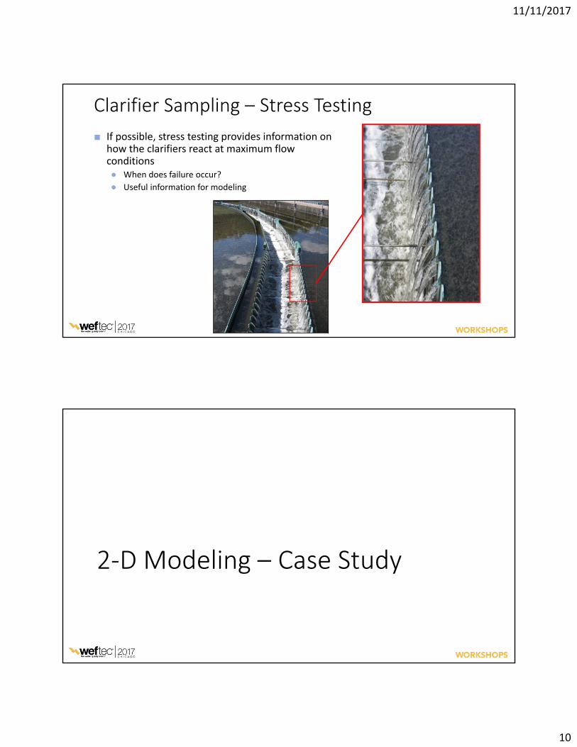
■ If possible, stress testing provides information onhow the clarifiers react at maximum flowconditions● When does failure occur?

● Useful information for modeling

11/11/2017

11

Developed at the University of New Orleans in 2004,

2Dc is a 2-D CFD model customized for clarifiers

• It account for all the major process occurring in settlingtanks (e.g., hydrodynamics, flocculation, environmentalimpacts)

• It accounts for the dynamics of the sludge inventory

• It can predict effluent quality and RAS concentration

• Allows visualization of the internal conditions in theclarifier, like position of the sludge blanket and flowpattern

• It incorporate the geometry and other internal featuresof the clarifiers

Concentration (g/L): 0.01 0.02 0.05 0.11 0.23 0.52 1.14 2.50 5.50

Radius = 60 ft

8.5 ft14.8 ft 14 ft

Slope = 8.33%

Concentration (g/L): 0.01 0.02 0.05 0.11 0.23 0.52 1.14 2.50 5.50

Radius = 60 ft

8.5 ft14.8 ft 14 ft

Slope = 8.33%

11/11/2017

12

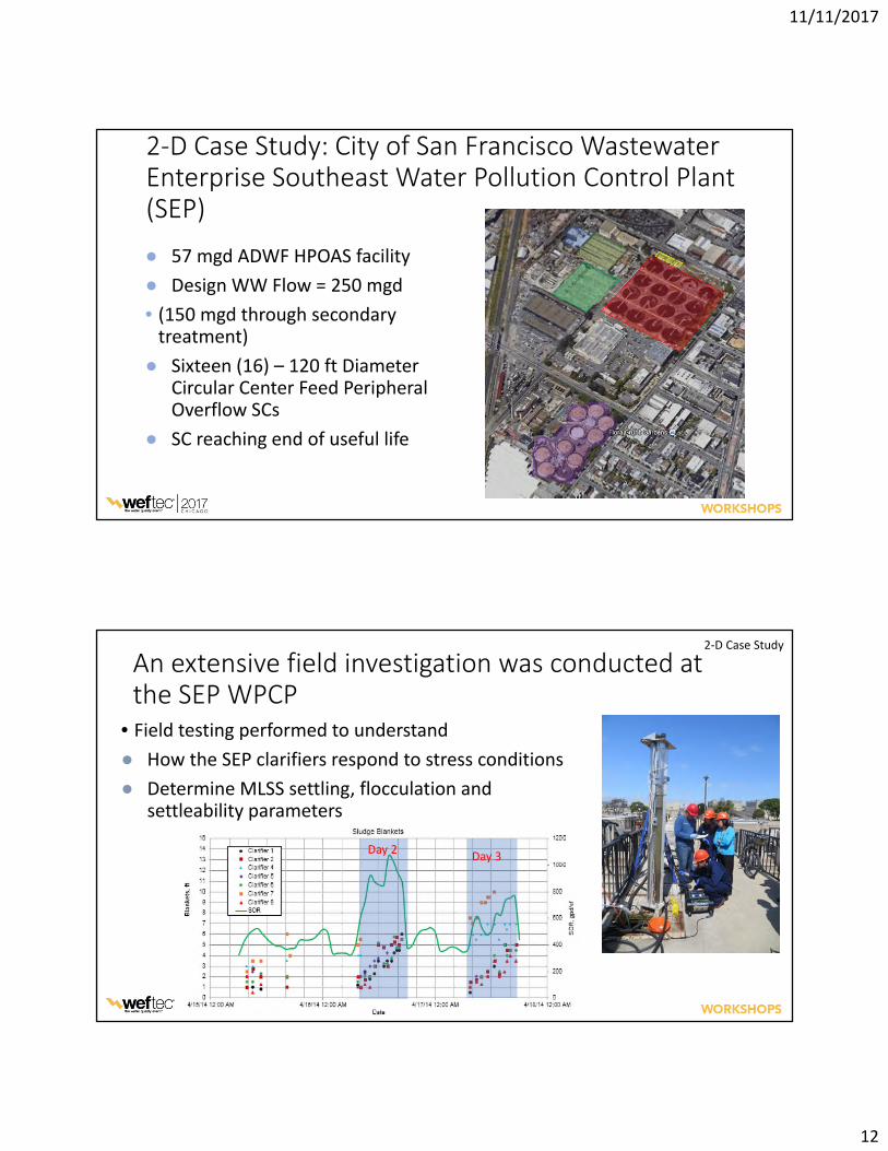
● 57 mgd ADWF HPOAS facility

● Design WW Flow = 250 mgd

• (150 mgd through secondarytreatment)

● Sixteen (16) – 120 ft DiameterCircular Center Feed PeripheralOverflow SCs

● SC reaching end of useful life

• Field testing performed to understand

● How the SEP clarifiers respond to stress conditions

● Determine MLSS settling, flocculation andsettleability parameters

Day 2Day 3

2-D Case Study

11/11/2017

13

The following data were collected and analyzed:

■ Stress Testing:

● Influent and effluent flows

● Return activated sludge flow rate

● MLSS, RAS SS, Effluent SS

● Sludge Blanket

● Sludge Volume Index

● Flocculation parameters

● Flocculated suspended solids (FSS)

● Dispersed suspended solids (DSS)

● Discrete settling parameters

● Settling properties of the sludge: zone, andcompression rates

■ Follow up testing

● Dye Studies

● RAS drawdown testing

● Stamford Baffle stress testing

● Microscopy

2-D Case Study

26

Clouds of solids are an indication of poor clarifierhydrodynamics (strong internal currents)

S ignificantcloudinessobservedw iththreeclarifiersonline SOR ≈ 1,000 gpd/ft2)

Cloudinessobservedw ithfourclarifiersonline SOR ≈ 850 gpd/ft2)

2-D Case Study

11/11/2017

14

SVI = 85 mL/g

Effluent TSS = 29.4 mg/LRAS TSS = 13,450 mg/L

720 Min

0.5 ft/s

● A computational fluid dynamics (CFD) modelwas developed and calibrated and validatedagainst stress testing data

● Model used to evaluate potential upgradesto be incorporated during clarifier rehab,including:

● Removal of inlet target baffles (were resulting infloc breakup)

● Center well diameter (existing too small)

● Stamford baffle position27

Effluent TSS = 30.5 m g/LRAS TSS = 13,500 mg/L

720 M

0.5 ft/s

Effluent TSS = 26.9 mg/LRAS TSS = 13,450 mg/L

720 Min

0.5 ft/sConc. (mg/L)

1000043291874811351152662812521

inutes

Center Well Diameter = 24-ft

Center Well Diameter = 36-ft

Center Well Diameter = 30-ft

2-D Case Study

28

45m g/L – W eeklyaverageO utfalleffluentlim itationduringdry w eather

20

25

30

35

40

45

50

55

60

65

70

140 150 160 170 180 190 200 210

Effl

ue

nt

TSS

(mg

/L)

Flow R ate-O neClarifierO utofS ervice(M GD)

Secondary Clarifier Capacity(MLSS = 2,800 mg/L, SVI = 85 mL/g, RAS = 30%)

Existing Clarifiers Retrofitted Clarifiers.

2-D Case Study

11/11/2017

15

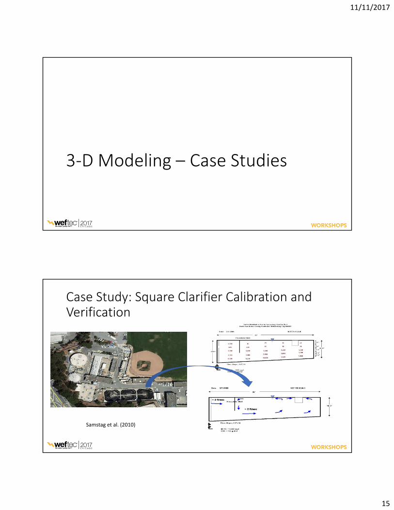
Samstag et al. (2010)

11/11/2017

16

S ettlingVelocity T ests DyeT ests

S olidsP rofileFieldT estCFD S im ulationVelocity andS olids

P rofile

11/11/2017

17

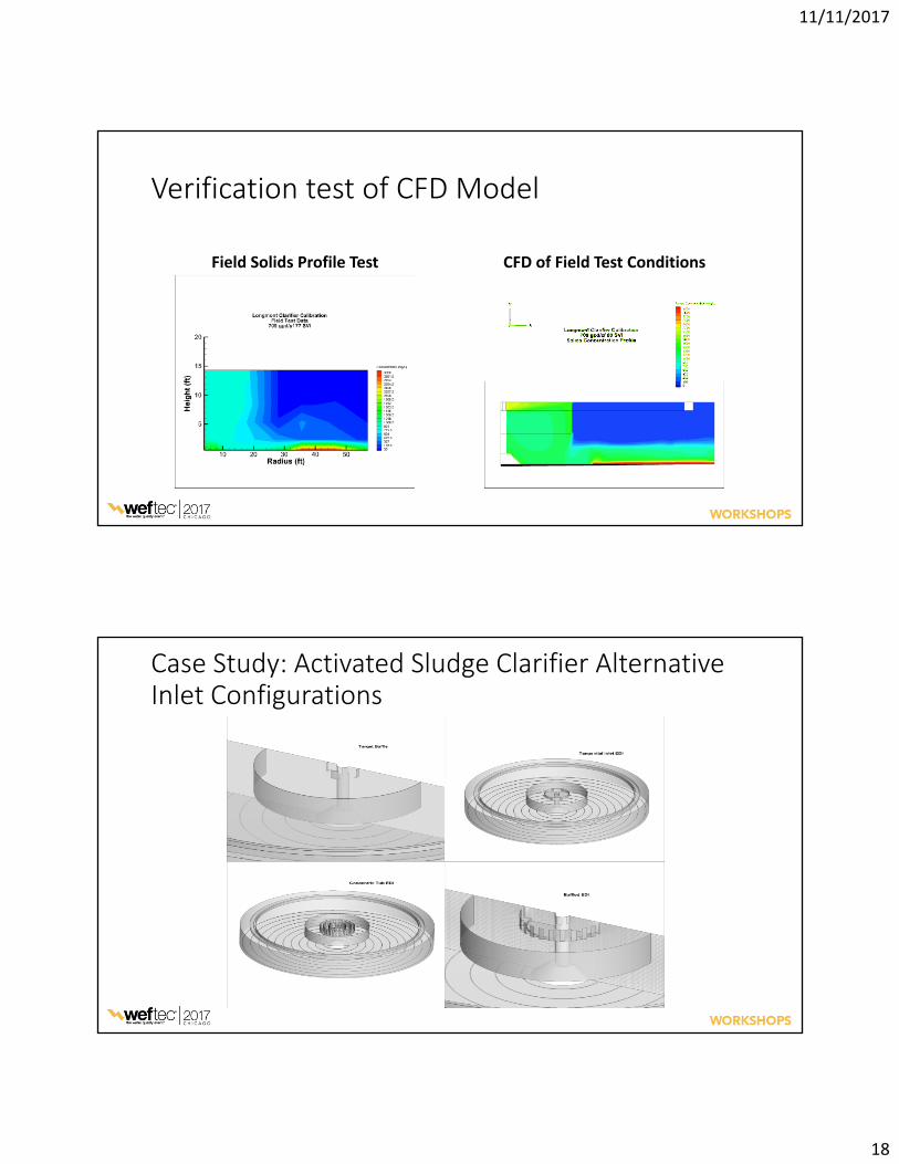
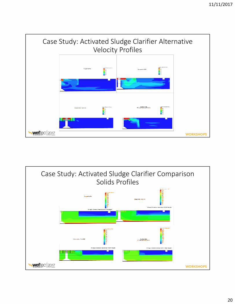
• Radial flow clarifier

• Questions:• Optimum Depth?

• Optimum Inlet ?

• Optimum Feedwell?

• Optimum Effluent Zone?

Samstag and Wicklein(2014)

• 3D Fluent CFD

• 1,100,000 hexahedral cells

• K-epsilon turbulence model

• User defined functions (UDF) toimplement

• Solids settling and transport

• Density coupling

11/11/2017

18

FieldS olidsP rofileT est CFD ofFieldT estConditions

11/11/2017

19

11/11/2017

20

11/11/2017

21

• It is still necessary to perform calibration and verification tests for CFDevaluation of sedimentation.

• Calibration test examples:• Settling tests

• Floc tests

• Verification test examples:• Solids profile tests

• Dye tests

• CFD can uncover significant potential capacity and performanceimprovements