Allocation subversion and

meta-analysis

Professor David Torgerson

Director, York Trials Unit

Department of Health Sciences

University of York

YORK United Kingdom

Allocation concealment

• Large amount of evidence (mainly from

health care trials) that randomisation is

often subverted

• Case studies of individual trials show this

to be the case

• Epidemiological studies of RCTs also

show statistical evidence of the problem

Comparison of concealment

Allocation Concealment

Effect Size OR

Adequate 1.0

Unclear 0.67 P < 0.01

Inadequate 0.59

Schulz et al. JAMA 1995;273:408.

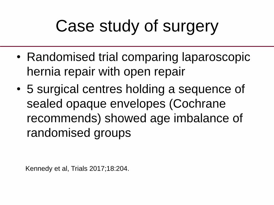
Case study of surgery

• Randomised trial comparing laparoscopic

hernia repair with open repair

• 5 surgical centres holding a sequence of

sealed opaque envelopes (Cochrane

recommends) showed age imbalance of

randomised groups

Kennedy et al, Trials 2017;18:204.

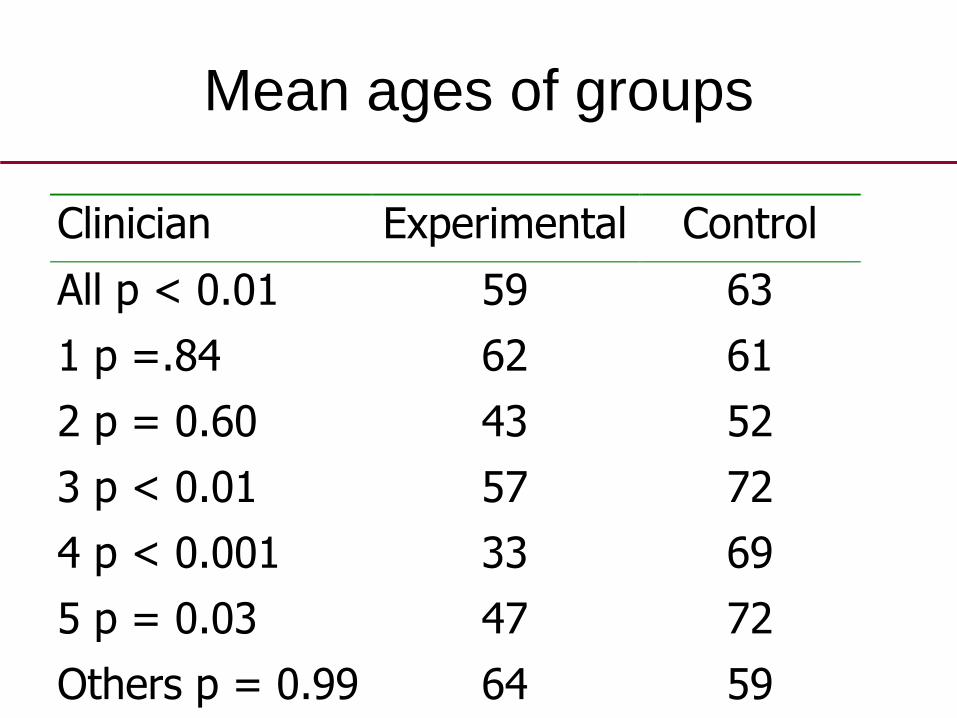
Mean ages of groups

Clinician Experimental Control

All p < 0.01 59 63

1 p =.84 62 61

2 p = 0.60 43 52

3 p < 0.01 57 72

4 p < 0.001 33 69

5 p = 0.03 47 72

Others p = 0.99 64 59

How did they do it?

0

5

10

15

20

25

30

1 3 5 7 9 11 13 15 17 19 21 23 25

Recruitment Sequence

En

ve

lop

e N

um

be

r

What is the problem here?

• There were 3 sites

• “Randomization was performed in

permuted blocks of two with the use of the

online tool Randomize.net, with

stratification according to site”

• 452 assigned to control group and 464 to

resistance group

Email correspondence

“Now it is me being v stupid confused or both. If you used a block of two stratified by site then the

allocation will be perfectly balanced at each site every 2 women. If recruitment finished mid way

through a block at each site then with 3 sites the biggest imbalance across the trial should be 3,

shouldn’t it?”

David

Dear David:You are correct that, when the randomization process works perfectly, the maximum imbalance when

stratified across 3 sites would be 3 subjects.

However, in practice, the computerized randomization process does not always work perfectly

because of the human element. In our trial on several occasions, the research assistants mistakenly

re-randomized subjects believing their online randomization had not been recorded or re-randomized

subjects in an attempt to correct spelling mistakes, or mistakenly sent subjects to the wrong session.

Despite the mistakes made at the time of randomization, none of the women were aware of their group

assignment at the time of signing informed consent or completing the baseline survey.

Note all 10 of misallocations fell into the intervention group

Statistical Evidence

• Hewitt and colleagues examined the association

between p values and adequate concealment in

4 major medical journals.

• Inadequate concealment largely used opaque

envelopes.

• The average p value for inadequately concealed

trials was 0.022 compared with 0.052 for

adequate trials (test for difference p = 0.045).

Hewitt et al. BMJ;2005: March 10th.

0

.05

.1.1

5

Den

sity

-10 -5 0 5logit (p-value)

Adequate Inadequate

Unclear

Systematic review of calcium for

weight loss• MSc student undertook a systematic

review of calcium supplements for weight

loss – comparing body weights at final

follow-up showed a statistically signficant

difference between the groups (-1.79 kg

favouring calcium group; p = 0.005).

• But there was also a difference of baseline

body weights.

Trowman et al. Br J of Nutrition 2006;95:1033-38

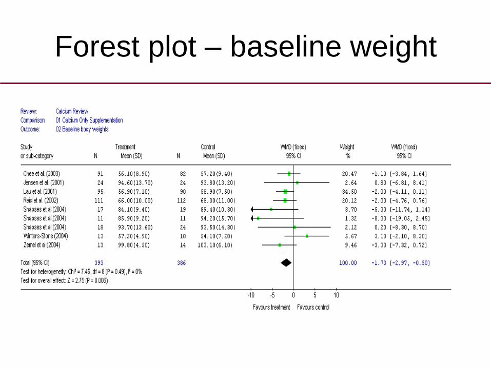
Forest plot – baseline weight

Symptoms of bias

• Baseline variables should be balanced

across trials. An individual trial might be in

imbalance by chance but meta-analysis of

several trials should generate an estimate

close to zero with no heterogeneity

• If there is heterogeneity and or imbalance

then some component trials could be

biased and the whole review is tainted

Review of Systematic Reviews

• 12 systematic reviews and meta-analyses

were identified from the four most cited

medical journals in 2012

• Meta-analysis of age was undertaken for

each systematic review

Clark et al. Journal of Clinical Epidemiology 2014: 67;1016-1024.

Why age?

• Two main reasons:

» Easy characteristic for someone to use to

subvert trial (e.g., older in control group)

» Most trial reports will produce, by group,

mean and SD of ages by allocated group

Age meta-analysis – arbitrary sample of 23

RCTs in health care

Difference = 0.005 (95% CI -0.026 to 0.035) I2 = 0%

Review results ranked by I2

Systematic

Review

Number of studies

available for MA

Area Intervention

age mean (SD)

Control age.

Mean (SD)

I squared

value

P-value of difference in

age

Anothaisintawe

e et al 2012 10

Drug

44.85 (5.56) 42.84 (5.67) 84.42 0.001

Rutjes et al

2012 38

Drug

62.17 (4.34) 62.44 (3.82) 67.92 0.835

Hemmingsen et

al 2012 14

Drug

58.07 (4.13) 58.54 (3.98) 53.03 0.156

Thangaratinam

et al 2012 20

Pregnancy and

childbirth 28.15 (2.27) 27.95 (2.05) 50.11 0.113

Umpierre et al

2011 26

Lifestyle

58.29 (4.27) 58.79 (4.44) 42.72 0.173

Neumann et al

2012 9

Drug

64.18 (2.45) 63.94 (2.94) 33.46 0.029

Heneghan et al

2011 8

Other

63.15 (7.61) 62.71 (9.11) 31.62 0.024

Palmer et al

2012 11

Drug

51.99 (8.35) 52.86 (8.95) 29.03 0.173

Orrow et al

2012 10

Lifestyle

62.57 (10.29) 62.82 (9.72) 16.18 0.736

Coombes et al

2010 18

Drug

48.08 (6.9) 48.08 (7.25) 0.00 0.362

Leucht et al

2012 21

Drug

40.31 (9.24) 39.92 (9.78) 0.00 0.008

Hempel et al

2012 26

Drug

41.84 (24.43) 42.19 (25.24) 0.00 0.818

Heterogeneity: age difference

Study name Statistics for each study Std diff in means and 95% CI

Std diff Standard Lower Upper in means error Variance limit limit Z-Value p-Value

Cheah 2003 0.145 0.216 0.047 -0.278 0.568 0.671 0.502

Bates 2007 0.377 0.445 0.198 -0.495 1.248 0.847 0.397

Nickel, downey et al 2004 2.731 0.348 0.121 2.050 3.412 7.857 0.000

leskinen 1999 0.080 0.364 0.132 -0.633 0.793 0.219 0.827

Shoskes 1999 0.181 0.366 0.134 -0.536 0.898 0.495 0.621

Nickel, Krieger et al 2008 0.000 0.121 0.015 -0.238 0.238 0.000 1.000

Alexander 2004 0.235 0.165 0.027 -0.089 0.559 1.421 0.155

Wagenlehner 2009 0.049 0.170 0.029 -0.284 0.381 0.288 0.774

Nicke, Downey, Clark et al 2003 -0.007 0.225 0.051 -0.449 0.435 -0.030 0.976

Pontari 2010 0.220 0.119 0.014 -0.013 0.452 1.850 0.064

0.198 0.060 0.004 0.081 0.315 3.307 0.001

-1.00 -0.50 0.00 0.50 1.00

Favours A Favours B

Meta Analysis

Meta Analysis

Difference in age p value = 0.001; I2 = 84.42

Heterogeneity: no age difference

Study name Statistics for each study Std diff in means and 95% CI

Std diff Standard Lower Upper in means error Variance limit limit Z-Value p-Value

Jackson 2011 -0.133 0.112 0.012 -0.352 0.086 -1.192 0.233

Hui 2004 0.000 0.299 0.089 -0.586 0.586 0.000 1.000

Barakat 2009 0.271 0.169 0.028 -0.059 0.602 1.608 0.108

Santos 2005 -0.544 0.240 0.058 -1.014 -0.073 -2.265 0.024

Hopkins 2010 0.566 0.206 0.042 0.162 0.969 2.746 0.006

Cavalcante 2009 0.266 0.239 0.057 -0.202 0.734 1.115 0.265

Hui 2011 0.253 0.146 0.021 -0.033 0.539 1.732 0.083

Haakstad 2011 0.221 0.196 0.038 -0.163 0.605 1.130 0.259

Garshasbi 2005 -0.045 0.137 0.019 -0.314 0.224 -0.328 0.743

Erkkola and Makela 1976 -0.083 0.237 0.056 -0.546 0.381 -0.349 0.727

Marquez-Sterling 1998 1.129 0.566 0.320 0.020 2.238 1.995 0.046

Baciuk 2008 0.266 0.239 0.057 -0.202 0.734 1.115 0.265

Crowther 2005 0.147 0.063 0.004 0.023 0.271 2.317 0.021

Phelan 2011 -0.038 0.100 0.010 -0.234 0.157 -0.385 0.700

Wolff 2008 -0.438 0.287 0.082 -1.000 0.125 -1.525 0.127

Khoury 2005 -0.056 0.118 0.014 -0.287 0.174 -0.480 0.632

Landon 2009 0.053 0.065 0.004 -0.074 0.180 0.821 0.411

Quinlivan 2011 -0.227 0.180 0.032 -0.581 0.126 -1.262 0.207

Asbee 2009 0.054 0.202 0.041 -0.342 0.450 0.265 0.791

Guelinckx 2010 -0.348 0.219 0.048 -0.776 0.081 -1.591 0.112

0.048 0.030 0.001 -0.011 0.107 1.583 0.113

-1.00 -0.50 0.00 0.50 1.00

Favours A Favours B

Meta Analysis

Meta Analysis

Difference in age p = 0.113; I2 = 50

Age imbalance no heterogeneity

Study name Statistics for each study Std diff in means and 95% CI

Std diff Standard Lower Upper in means error Variance limit limit Z-Value p-Value

Arato 2002 0.154 0.138 0.019 -0.116 0.424 1.120 0.263

Beasley 2003 0.103 0.120 0.014 -0.131 0.337 0.864 0.388

Boonstra 2011 0.033 0.449 0.202 -0.848 0.914 0.073 0.942

Clark 1975 0.136 0.365 0.134 -0.581 0.852 0.371 0.711

Cooper 2000 0.112 0.184 0.034 -0.247 0.472 0.613 0.540

Crow 1986 0.381 0.185 0.034 0.018 0.744 2.060 0.039

Gross 1974 0.120 0.273 0.075 -0.415 0.655 0.440 0.660

Hirsch 1973 0.166 0.223 0.050 -0.270 0.602 0.745 0.456

Hirsch 1996 -0.122 0.238 0.056 -0.587 0.344 -0.512 0.609

Kane 2011 0.041 0.102 0.010 -0.158 0.241 0.407 0.684

Kane 1979 -0.073 0.500 0.250 -1.054 0.907 -0.146 0.884

Kane 1982 -0.137 0.387 0.150 -0.896 0.622 -0.354 0.724

Kramer 2007 0.142 0.140 0.020 -0.132 0.416 1.016 0.310

Kurland 1975 -0.372 0.341 0.116 -1.041 0.297 -1.090 0.276

Nishikawa 1984 -0.093 0.212 0.045 -0.509 0.323 -0.437 0.662

Levine 1980 0.071 0.301 0.090 -0.519 0.660 0.235 0.814

Peuskens 2007 0.578 0.156 0.024 0.272 0.884 3.705 0.000

Sampath 1992 -0.090 0.408 0.167 -0.890 0.711 -0.219 0.826

Vandecasteele 1974 -0.028 0.437 0.191 -0.884 0.828 -0.064 0.949

Wistedt 1981 -0.158 0.329 0.108 -0.803 0.487 -0.479 0.632

Zissis 1982 -0.118 0.354 0.125 -0.812 0.576 -0.334 0.739

0.117 0.044 0.002 0.030 0.203 2.645 0.008

-1.00 -0.50 0.00 0.50 1.00

Favours A Favours B

Meta Analysis

Meta Analysis

Difference in age (p = 0.008;) hetererogeneity = 0.00

How it should be!

Study name Statistics for each study Std diff in means and 95% CI

Std diff Standard Lower Upper

in means error Variance limit limit Z-Value p-Value

Borgia 1982 -0.115 0.224 0.050 -0.553 0.324 -0.512 0.609

Beausoleil 2007 -0.294 0.213 0.045 -0.712 0.124 -1.378 0.168

Song 2010 0.064 0.137 0.019 -0.204 0.333 0.471 0.638

de Bortoli 2007 0.087 0.139 0.019 -0.186 0.361 0.627 0.531

Wenus 2008 0.148 0.215 0.046 -0.274 0.570 0.688 0.491

McFarland 1995 -0.095 0.144 0.021 -0.377 0.187 -0.659 0.510

Correa 2005 -0.023 0.160 0.025 -0.336 0.290 -0.147 0.884

Jirapinyo 2002 0.320 0.477 0.228 -0.616 1.256 0.670 0.503

Park 2007 -0.125 0.107 0.011 -0.334 0.084 -1.174 0.240

Felley 2001 0.008 0.278 0.077 -0.536 0.552 0.030 0.976

Duman 2005 0.078 0.102 0.010 -0.122 0.277 0.763 0.445

Szymanski 2008 0.107 0.227 0.051 -0.337 0.552 0.474 0.635

Thomas 2001 0.158 0.123 0.015 -0.082 0.398 1.290 0.197

Safdar 2008 -0.449 0.324 0.105 -1.084 0.185 -1.387 0.165

Kotowska 2005 0.069 0.122 0.015 -0.171 0.308 0.562 0.574

Schrezenmeir 2004 0.112 0.218 0.047 -0.315 0.539 0.513 0.608

Yoon 2011 -0.109 0.110 0.012 -0.324 0.106 -0.997 0.319

Hickson 2007 -0.018 0.172 0.030 -0.356 0.319 -0.107 0.914

Conway 2007 -0.016 0.120 0.014 -0.251 0.218 -0.137 0.891

Lewis 1998 -0.622 0.247 0.061 -1.106 -0.139 -2.522 0.012

Koning 2008 -0.314 0.371 0.137 -1.040 0.413 -0.846 0.397

Song 2010 -0.007 0.078 0.006 -0.159 0.146 -0.089 0.929

Szajewska 2009 0.138 0.220 0.048 -0.293 0.570 0.628 0.530

Merenstein 2009 -0.214 0.179 0.032 -0.566 0.138 -1.193 0.233

Ruszczynski 2008 0.030 0.129 0.017 -0.224 0.283 0.229 0.819

Sampalis 2010 0.075 0.096 0.009 -0.112 0.263 0.786 0.432

-0.007 0.028 0.001 -0.062 0.049 -0.231 0.818

-1.00 -0.50 0.00 0.50 1.00

Favours A Favours B

Difference in age p = 0.81; I2 = 0.00

Comment

• Out of 12 meta-analyses published in 4

leading medical journals:

» Only 3 showed the expected zero

heterogeneity and zero imbalance

A review conclusion

• In the review with >50% I2 it was

concluded that:

» Dietary and lifestyle interventions can reduce

maternal gestational weight gain and improve

outcomes for both mother and baby

• Is such a result believable – given the

likelihood of biased trials?

Comments from

reviewers/researchers• Perhaps some characteristics of setting

intervention affects heterogeneity

» Bonkers

• But the baseline difference is non-

existence/clinically irrelevant

» But this is a marker for subversion some other

unreported co-variate might be worse!

• Could it be due to publication bias?

» Don’t think so

Anti-body exposure to ‘flu

Ebell 2013; Methodological concerns about studies on oseltamivir

for flu (BMJ 2013;347:f7148)

Comment

• We have a BIG problem – the evidence

suggests significant numbers of subverted

trials are entering the ‘food chain’

• Unless we scrap all the evidence of the

last 50 years and start again what can we

do?

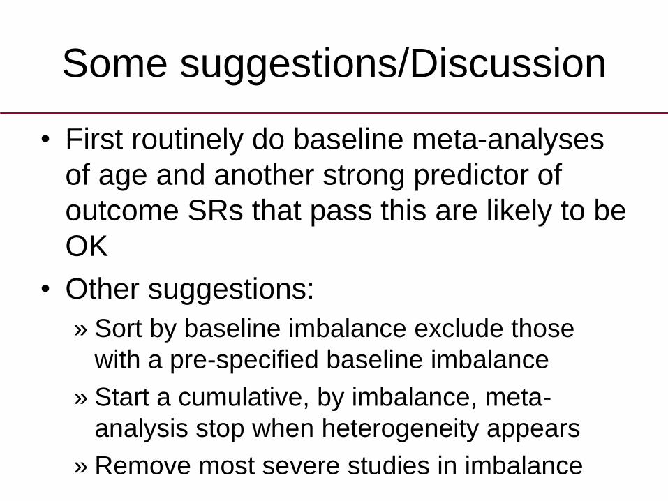
Some suggestions/Discussion

• First routinely do baseline meta-analyses

of age and another strong predictor of

outcome SRs that pass this are likely to be

OK

• Other suggestions:

» Sort by baseline imbalance exclude those

with a pre-specified baseline imbalance

» Start a cumulative, by imbalance, meta-

analysis stop when heterogeneity appears

» Remove most severe studies in imbalance

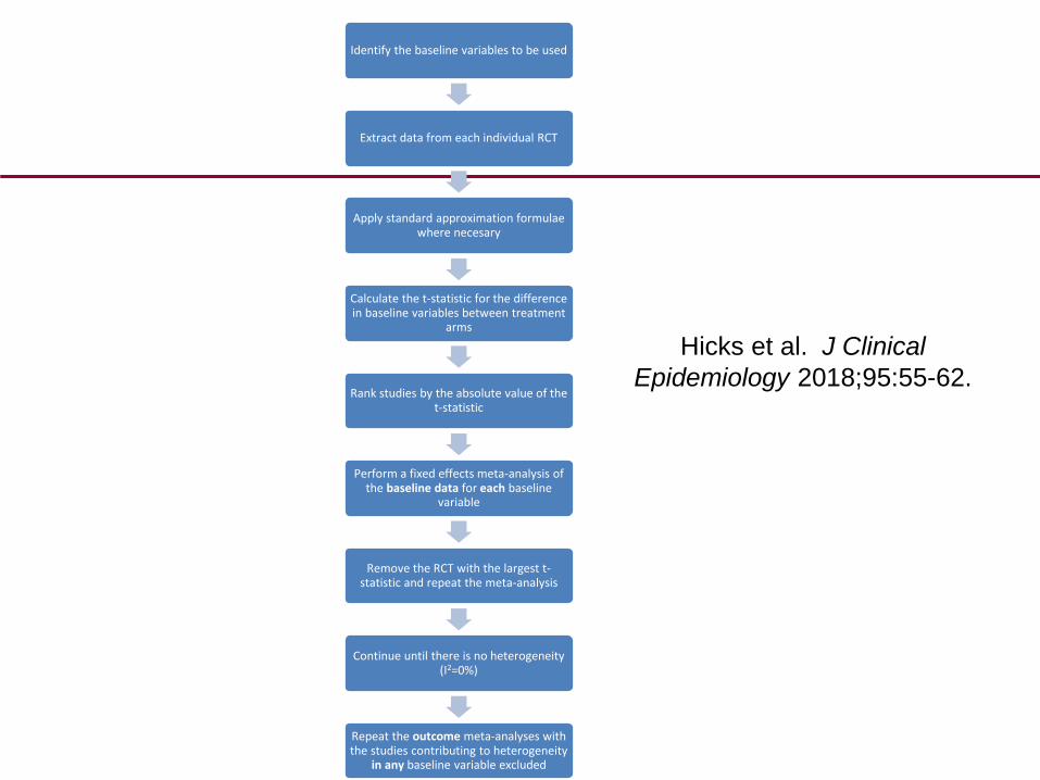
Identify the baseline variables to be used

Extract data from each individual RCT

Apply standard approximation formulae where necesary

Calculate the t-statistic for the difference in baseline variables between treatment

arms

Rank studies by the absolute value of the t-statistic

Perform a fixed effects meta-analysis of the baseline data for each baseline

variable

Remove the RCT with the largest t-statistic and repeat the meta-analysis

Continue until there is no heterogeneity (I2=0%)

Repeat the outcome meta-analyses with the studies contributing to heterogeneity

in any baseline variable excluded

Hicks et al. J Clinical

Epidemiology 2018;95:55-62.

Study Mean Difference (kg) t-statistic absolute value of t-statistic

Heterogeneitya I2 (%)

(35.4% total)

Hopkins 2 2.618964 2.618964 29.3

Crowther 0.8 2.319949 2.319949 25.5

Santos -2.6 -2.306597 2.306597 12.8

Marquez-Sterling 3.5 2.142188 2.142188 1.07

Hui 1.4 1.738516 1.738516 0.0

Clapp 1 1.732051 1.732051 0.0

Barakat 0.9 1.615753 1.615753 0.0

Guelinckx -1.4 -1.603391 1.603391 0.0

Wolff -2 -1.542686 1.542686 0.0

Barakat 1 1.294297 1.294297 0.0

Quinlivan -1.2 -1.265797 1.265797 0.0

Jackson -0.8 -1.193001 1.193001 0.0

Haakstad 0.9 1.133327 1.133327 0.0

Baciuk 1.4 1.120274 1.120274 0.0

Erkkola 0.4 1.025268 1.025268 0.0

Landon 0.3 0.821535 0.821535 0.0

Bung -1 -0.625135 0.625135 0.0

Khoury -0.2 -0.479653 0.479653 0.0

Phelan -0.2 -0.385095 0.385095 0.0

Erkkola + Makela 0.2 0.368133 0.368133 0.0

Garshasbi -0.21 -0.328250 0.328250 0.0

Asbee 0.3 0.265534 0.265534 0.0

Huang 0.22 0.262568 0.262568 0.0

Khaledan 0.15 0.093955 0.093955 0.0

Sedaghati 0.02 0.026337 0.026337 0.0

Huib 0 0 0 0.0

Vinterb 0 0 0 0.0

aheterogeneity observed in meta-analysis of baseline age when this study (and those with higher t-statistic) removed

bstudies with same t-statistic ranked according to sample size (largest first)

Studies in meta-analysis ranked by t value of age difference

Cluster trials

• Many cluster trials (where a group is the

unit of randomisation e.g., schools) recruit

individual participants after randomisation

has occurred

• This is essentially ‘open’ allocation and

biased recruitment can take place as

within individual randomised trials

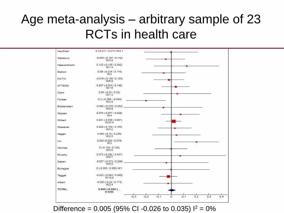
Age meta-analysis – arbitrary sample of 23

RCTs in health care

Difference = 0.005 (95% CI -0.026 to 0.035) I2 = 0%

Cluster trials any better?

Difference in age: -0.05 (95% CI -0.057 to -0.0426) I2 = 93.2%

Bolzern et al, J Clinical Epidemiology 2018;99:106-112.

Conclusion

• Significant proportion of randomised trials,

in health care, are ‘subverted’ and are not

really randomised

• This subversion feeds into meta-analyses

results

• The same problem will apply to non-health

care trials – therefore the same

identification technique might be useful