algorithms for return probabilities for stochastic fluid flows
TRANSCRIPT

This article was downloaded by: [Ryerson University]On: 10 October 2014, At: 09:25Publisher: Taylor & FrancisInforma Ltd Registered in England and Wales Registered Number: 1072954 Registeredoffice: Mortimer House, 37-41 Mortimer Street, London W1T 3JH, UK
Stochastic ModelsPublication details, including instructions for authors andsubscription information:http://www.tandfonline.com/loi/lstm20
ALGORITHMS FOR RETURN PROBABILITIESFOR STOCHASTIC FLUID FLOWSNigel G. Bean a , Małgorzata M. O'Reilly b & Peter G. Taylor c
a Applied Mathematics , University of Adelaide , South Australia,Australiab Applied Mathematics , University of Adelaide, South Australia,Australia and Department of Mathematics and Statistics, Universityof Melbourne , Victoria, Australiac Department of Mathematics and Statistics , University ofMelbourne , Victoria, AustraliaPublished online: 02 Sep 2006.
To cite this article: Nigel G. Bean , Małgorzata M. O'Reilly & Peter G. Taylor (2005) ALGORITHMSFOR RETURN PROBABILITIES FOR STOCHASTIC FLUID FLOWS, Stochastic Models, 21:1, 149-184, DOI:10.1081/STM-200046511
To link to this article: http://dx.doi.org/10.1081/STM-200046511
PLEASE SCROLL DOWN FOR ARTICLE
Taylor & Francis makes every effort to ensure the accuracy of all the information (the“Content”) contained in the publications on our platform. However, Taylor & Francis,our agents, and our licensors make no representations or warranties whatsoever as tothe accuracy, completeness, or suitability for any purpose of the Content. Any opinionsand views expressed in this publication are the opinions and views of the authors,and are not the views of or endorsed by Taylor & Francis. The accuracy of the Contentshould not be relied upon and should be independently verified with primary sourcesof information. Taylor and Francis shall not be liable for any losses, actions, claims,proceedings, demands, costs, expenses, damages, and other liabilities whatsoever orhowsoever caused arising directly or indirectly in connection with, in relation to or arisingout of the use of the Content.
This article may be used for research, teaching, and private study purposes. Anysubstantial or systematic reproduction, redistribution, reselling, loan, sub-licensing,systematic supply, or distribution in any form to anyone is expressly forbidden. Terms &Conditions of access and use can be found at http://www.tandfonline.com/page/terms-and-conditions
Stochastic Models, 21(1):149–184, 2005Copyright © Taylor & Francis, Inc.ISSN: 1532-6349 print/1532-4214 onlineDOI: 10.1081/STM-200046511
ALGORITHMS FOR RETURN PROBABILITIES FOR STOCHASTIC
FLUID FLOWS
Nigel G. Bean � Applied Mathematics, University of Adelaide, South Australia,Australia
Małgorzata M. O’Reilly � Applied Mathematics, University of Adelaide, SouthAustralia, Australia and Department of Mathematics and Statistics, University ofMelbourne, Victoria, Australia
Peter G. Taylor � Department of Mathematics and Statistics, University ofMelbourne, Victoria, Australia
� We consider several known algorithms and introduce some new algorithms that can beused to calculate the probability of return to the initial level in the Markov stochastic fluidflow model. We give the physical interpretations of these algorithms within the fluid flowenvironment. The rates of convergence are explained in terms of the physical properties ofthe fluid flow processes. We compare these algorithms with respect to the number of iterationsrequired and their complexity. The performance of the algorithms depends on the nature ofthe process considered in the analysis. We illustrate this with examples and give appropriaterecommendations.
Keywords Asmussen’s iteration; Fixed-point iterations; Latouche-Ramaswamimethod; Markovian fluid model; Newton’s method; Return probabilities.
Mathematics Subject Classification 60J25; 60617.
1. INTRODUCTION
Fluid flow models of the class considered in this paper were studiedby, for example, Anick, Mitra and Sondhi[2], Asmussen[3], Ramaswami[21],Rogers[22], da Silva Soares and Latouche[9], and Ahn and Ramaswami[1].In these models, the rate, ci, at which the level of a fluid increases,or decreases, is governed by the state i of the underlying continuous-time Markov chain. The parameters, ci, can be positive, negative or
Received March 2004; Accepted September 2004Address correspondence to Nigel G. Bean, Applied Mathematics, University of Adelaide,
SA 5005, Australia; E-mail: [email protected]
Dow
nloa
ded
by [
Rye
rson
Uni
vers
ity]
at 0
9:25
10
Oct
ober
201
4
150 Bean, O’Reilly, and Taylor
zero. Recently, Ref.[6], we established expressions for several performancemeasures for this class of models. In this paper, we shall describe andanalyze algorithms that can be used to calculate return probabilities to theinitial level, from which all performance measures defined in Ref.[6] canbe derived. We shall simplify the general fluid flow model by assumingci to be 1 or −1, because as shown in Refs.[3,6,22], general models canbe transformed into such a model while preserving return probabilities.Such a simplified fluid flow model is a two-dimensional continuous-timeuncountable-level finite-phase Markov process, denoted by �(X(t),�(t)) :t ∈ �+�, where
• the level is denoted by X(t) ∈ �+,• the phase is denoted by �(t) ∈ � = �1 ∪ �2,• the phase process ��(t) : t ∈ �+� is an irreducible Markov chain with
infinitesimal generator � , and• the net rate of input ci to the infinite fluid buffer, when �(t) is in state i,
is equal to 1 for i ∈ �1 and −1 for i ∈ �2.
We partition the infinitesimal generator according to � = �1 ∪ �2
so that
� =[
T11 T12
T21 T22
]and let s1 = |�1|, s2 = |�2|.
Assume that the process (X(t),�(t)) starts from level x in phase i ∈ �1
at time 0. Let �(x) = inf�t > 0 : X(t) = x� be the first passage time tolevel x. For i ∈ �1 and j ∈ �2, let
�ij = P[�(x) < ∞,�(�(x)) = j | X(0) = x,�(0) = i], (1)
and � = [�ij]. In physical terms, �ij is the probability that, starting fromlevel x in phase i ∈ �1, the process (X(t),�(t)) first returns to level x infinite time and does so in phase j ∈ �2, while avoiding levels below x. Thematrix � records return probabilities to the initial level for all such i, j.We have dropped the subscript x from the notation, as these probabilitiesdo not depend on the starting level in this upwardly homogenous process.Without loss of generality, we shall often assume that the process startsfrom level zero at time 0.
By Ref.[6], the matrix analogous to � , defined for the general modelin which rates ci can take any value in �, can be calculated from thecorresponding matrix in this simplified model. The matrix � appearsin expressions for other measures of the process (see for exampleRefs.[6,9,21]) and consequently, calculation of � is an obvious first step
Dow
nloa
ded
by [
Rye
rson
Uni
vers
ity]
at 0
9:25
10
Oct
ober
201
4
Algorithms for Stochastic Fluid Flows 151
that has become the focus of research. It has been determined inRefs.[6,22,25] that the matrix � is the minimal non-negative solution of thenonsymmetric algebraic Riccati equation,
T11� + � T22 + � T21� + T12 = 0. (2)
A number of methods that can be used to solve this equation have beenreported by Guo[13]. Asmussen[3] established algorithms for � by using analternative approach. A further method was proposed by Ramaswami[21],who related the fluid process to a discrete-level quasi-birth-and-deathprocess (QBD). This allows one to calculate � using any algorithmsavailable for QBDs, such as the Logarithmic Reduction algorithm ofLatouche and Ramaswami[19] or the Cyclic Reduction algorithm of Biniand Meini[8]. In this paper, we introduce two new algorithms, andanalyze the above-mentioned algorithms with respect to their physicalinterpretation, complexity and convergence properties. The performanceof the algorithms, which depends on the physical properties of theprocess, is illustrated with examples. We make recommendations inrelation to which method is best in which circumstances.
This paper is organized as follows: Section 2 contains a briefdescription of the methods, which are then compared in Section 3via physical interpretations. In Section 4 we show that the algorithmsconverge to � and compare them with respect to the number of iterationsrequired. Results on the rates of convergence are given in Section 5.In Section 6 we compare the numerical complexity of the algorithms.The examples in Section 7 focus on the overall performance of thesealgorithms. This is followed by concluding remarks in Section 8.
For p × q matrices A and B, we shall write A < B if Aij < Bij for alli ∈ �1, � � � , p�, j ∈ �1, � � � , q�, with similar definitions for >, ≤, ≥, and =. Weshall write A �= B if A = B is not satisfied. We shall use the notation At forthe transpose of the matrix A and 0 for the zero matrix of an appropriatesize. When necessary, we shall indicate that 0 is a square matrix of orders1 or s2 with the notation 011 or 022, respectively. Similarly, I11 and I22 shallbe the identity matrices of order s1 and s2, respectively, and e a vector ofones of appropriate size.
2. ALGORITHMS
Before we refer to known methods, we note that by the simple action ofwriting equation (2) in a different form and then introducing an iteration,several algorithms for � can be obtained. For example, we can write (2) as
T11� + � T22 = −T12 − � T21� .
Dow
nloa
ded
by [
Rye
rson
Uni
vers
ity]
at 0
9:25
10
Oct
ober
201
4
152 Bean, O’Reilly, and Taylor
A corresponding iteration can be obtained by setting �0 = 0, and thenusing
T11�n+1 + �n+1T22 = −T12 − �nT21�n (3)
to calculate subsequent values of �n. In a similar manner, we can obtainthree more iterations. In each, we start the iteration with the matrix 0. The(n + 1)-st iteration is given, respectively, by the equations
T11�n+1 + �n+1(T22 + T21�n) = −T12, (4)
(T11 + �nT21)�n+1 + �n+1T22 = −T12, (5)
(T11 + �nT21)�n+1 + �n+1(T22 + T21�n) = −T12 + �nT21�n. (6)
The notation �n+1, �n+1, �n+1 and �n+1 reflects the fact that theEquations (3)–(6) define different iterations. Alternative versions of theiterations (3)–(6), with a nonzero matrix in the 0-th iteration, could alsobe considered, but this is beyond the scope of this paper. All of (3)–(6)are equations of type AX + XB = C. These can be solved using the Bartels-Stewart algorithm[4] or the Hessenberg-Schur method[11].
Guo[13] analyzed several methods which can be used to find theminimal nonnegative solution of Equation (2): fixed-point iterations,Newton’s method and the Schur method. The Schur method, which isnot an iterative method, but an approximation, is not considered here.We note however, that this approximation can be used to replace the 0-thiteration of the iterations (3)–(6) and can considerably reduce the com-putational cost, as pointed out by Guo[13] in relation to Newton’s method.Guo’s fixed-point iteration FP3 is the only fixed-point iteration worth con-sidering, as it is the fastest in terms of the number of iterations[13].Fixed-point iteration FP3 and Newton’s method[13] are equivalent in ourmodel to the iterations (3) and (6) respectively. We shall refer to theiterations (4) and (5) as the First-Exit algorithm and the Last-Entrancealgorithm respectively. The reason for this choice of names will becomeapparent in Section 3, when we present their physical interpretations.
In Ref.[21], Ramaswami related the fluid process to a discrete timeQBD, which allows for efficient calculation of � by existing algorithms[8,19].da Silva Soares and Latouche[9] gave a probabilistic interpretation of thisconstruction. We give a brief summary of this interpretation in Section 3.We shall refer to the method that consists of the QBD construction[21]
and the Logarithmic Reduction algorithm[19] as the Latouche-Ramaswamimethod. The method, which consists of the QBD construction[21] andthe Cyclic Reduction algorithm[8], shall be referred to as the Bini-Meini-Ramaswami method. Because these two methods are similar, we shall discussthe physical interpretation of the Latouche-Ramaswami method only.
Dow
nloa
ded
by [
Rye
rson
Uni
vers
ity]
at 0
9:25
10
Oct
ober
201
4
Algorithms for Stochastic Fluid Flows 153
However, numerical implementations of both the Latouche-Ramaswamiand the Bini-Meini-Ramaswami method will be compared with the abovementioned algorithms in Section 7.
Asmussen[3] proposed three iteration schemes that can be used tocalculate � and which, unlike Ramaswami’s construction, operate withinthe stochastic fluid environment. However, he gave no numerical analysisof these schemes. We shall refer to the first scheme, Theorem 3.1, asAsmussen’s iteration[3]. In Section 3 we give the physical interpretation ofthis iteration. The second scheme, Theorem 3.2, can require many moreiterations than the first, as pointed out by Asmussen and confirmed by ournumerical experience[3]. For this reason, we shall not discuss it here.
The third scheme, Theorem 3.3[3], requires calculation of the inverseof a Kronecker sum[12] at each step of the scheme, which is inefficientnumerically. However, the equation in Theorem 3.3[3], underlying thisiteration scheme, can be shown to be equivalent to (4). This can be donein two steps. First, convert (4) into the equivalent form
vec �n+1 = −[(T22 + T21�n)t ⊕ T11]−1vec T12, (7)
where A ⊕ B is a Kronecker sum[12] of matrices A and B, and vec A[12] isan ordered stack of the columns of A. Second, observe that the equationin Theorem 3.3[3] of Ref.[3] (after correcting for the missing minus signthere), is equivalent to (7). In the First-Exit algorithm, the (n + 1)-stiteration is obtained by solving Equation (4), using the Bartels-Stewartalgorithm[4]. We shall analyze this improved form here.
3. PHYSICAL INTERPRETATIONS
We start by rewriting Equations (3)–(6) in a form, that is moreconvenient for physical interpretation. This is given in the followinglemma.
Lemma 1. Equations (3) to (6) are equivalent to
�n+1 =∫ ∞
0eT11y(T12 + �nT21�n)eT22ydy, (8)
�n+1 =∫ ∞
0eT11yT12e(T22+T21�n)ydy, (9)
�n+1 =∫ ∞
0e(T11+�nT21)yT12eT22ydy, (10)
�n+1 = ∫ ∞0 e(T11+�nT21)y(T12 − �nT21�n)e(T22+T21�n)ydy. (11)
Dow
nloa
ded
by [
Rye
rson
Uni
vers
ity]
at 0
9:25
10
Oct
ober
201
4
154 Bean, O’Reilly, and Taylor
Furthermore, for fixed �n, �n, �n and �n, each of the Equations (3)–(6) have aunique solution.
Proof. In this proof we shall use the notation �n+1, �n+1, �n+1 and �n+1
to denote only the matrices defined in (8)–(11). The proof of theequivalence of (8)–(11) to (3)–(6) respectively, follows by Theorem 9.2 inRef.[7] and the fact that eigenvalues with the maximum real part of eachof the matrices T11, T22, (T22 + T21�n), (T11 + �nT21), (T11 + �nT21) and(T22 + T21�n) are negative. This was follows by Lemma 3 of Ref.[6] for thefirst two matrices. The proof for the remaining matrices is analogous.
In Theorem 2 below, we show that the matrices �n, �n, �n and �n
converge to � as n → ∞. By taking limits as n → ∞ in Equations (8)–(11)we obtain three known expressions for � [6,9,21] and the new expression
� =∫ ∞
0e(T11+�T21)y(T12 − � T21�)e(T22+T21�)y dy.
We shall see that, at each iteration of the algorithms (8)–(11) (with a zeromatrix assumed at the 0-th step) the matrix records the total probabilitymass of certain sample paths, but not others. We shall refer to the setsof sample paths that contribute to �n, �n, �n and �n, respectively as �n,�n, �n and �n. When a sample path starts and finishes at some levelw different than level zero, we shall call it a sample path in (say) �n
shifted to level w. Our analysis shall lead to the determination of exactlywhich sample paths lie in each of �n, �n, �n and �n via useful physicalinterpretations. Later, in Section 4, we shall use these interpretations tocompare the algorithms with respect to the number of iterations required.
The physical interpretation of Newton’s method[13] was previouslyunknown. Another novel aspect is our physical interpretation of theLatouche-Ramaswami method. Da Silva Soares and Latouche[9] gave aphysical interpretation of the QBD that is constructed in Ref.[21]. Ourcontribution is the physical interpretation of the nth iteration of theLogarithmic Reduction algorithm[19] applied to such a construction, interms of a transformed fluid model.
The Cyclic Reduction algorithm[8] has a lower computational cost periteration than the Logarithmic Reduction algorithm[19], as the formerrequires six matrix multiplications and one matrix inversion while thelatter requires eight matrix multiplications and one matrix inversion perstep[8]. The physical interpretations of the two algorithms, in the QBDenvironment, are similar. Both the Cyclic Reduction and the LogarithmicReduction algorithm calculate the matrix G, from which � can bedetermined.
With a ‘‘fair’’ counting of the number of iterations (the first iterationto include those sample paths that start at level 1 and hit level 0
Dow
nloa
ded
by [
Rye
rson
Uni
vers
ity]
at 0
9:25
10
Oct
ober
201
4
Algorithms for Stochastic Fluid Flows 155
without reaching level 2), the k-th iteration in the Logarithmic Reductionalgorithm is the approximation of the matrix G, incorporating all pathsstarting from level n that do not visit level n + 2k − 1 or above, while thek-th iteration of the Cyclic Reduction algorithm is the approximation ofthe matrix G, incorporating all paths starting from level n that do notvisit level n + 2k−1 or above. Thus, it is likely that the Cyclic Reductionalgorithm will take one more iteration than the Logarithmic Reductionalgorithm to reach a desired degree of accuracy. However, this extraiteration is likely to be compensated for in terms of the per-iterationefficiency of the Cyclic Reduction algorithm and we can conclude that thisalgorithm will use less CPU time in most cases. We shall expand on this inSection 6.
3.1. Fixed-Point Iteration FP3
Let the matrix P(k) be such that [P(k)]ij is the probability that, startingfrom phase i, the process first returns to the initial level in finite time, doesso in phase j, and there are exactly k transitions from �1 to �2 (or peaks)during this journey. We have
�ij =∞∑
k=1
[P(k)]ij.
Conditioning analogous to the one outlined below, was introduced inRef.[6] to derive the Laplace-Stieltjes transform of the time taken toreturn to the initial level, for a general model. By conditioning on themaximum fluid level reached and by (8), we have
P(1) = �1 =∫ ∞
0eT11yT12eT22ydy. (12)
For n ≥ 1, consider the paths in the set �n+1. By (8),
�n+1 = �1 +∫ ∞
0eT11w�nT21�neT22wdw, (13)
and so �1 ⊂ �n+1. Moreover, with w defined as
w = inf�x : transition �2 → �1 occurs at level x�, (14)
�n+1 includes every path that has the following physical interpretation:
• Starting from level zero in phase i at time 0, the phase process remainsin the set �1, until the fluid level reaches w in some phase k ∈ �1.
Dow
nloa
ded
by [
Rye
rson
Uni
vers
ity]
at 0
9:25
10
Oct
ober
201
4
156 Bean, O’Reilly, and Taylor
Because the net input rates in �1 are 1, this happens at time w. Theprobability of this is [eT11w]ik.
• Then, a sample path in �n shifted to level w, ending in some k′ ∈ �2,occurs.
• Next, a transition from k′ ∈ �2 to some l′ ∈ �1 occurs at level w. Thishappens at a rate [T21]k′l′ .
• Next, a sample path in �n shifted to level w, starting in l′ and ending inl, occurs.
• Finally, the phase process remains in the set �2 until the fluid level firstreturns to level 0 and does so in phase j ∈ �2. Because the net inputrates in �2 are −1, the duration of time spent in �2 during this stage ofthe process is w. The probability of this is [eT22w]lj.
From this physical interpretation, we are able to deduce some usefulinformation about the number of peaks in a sample path contributing tothe nth iteration of FP3. This is established in the form of the inequalitybelow.
Lemma 2. For n ≥ 1, the matrix �n satisfies
n∑k=1
P(k) ≤ �n ≤2n−1∑k=1
P(k). (15)
Proof. Let �n be the maximum number of peaks of a sample path in �n,starting in some i ∈ �1 and finishing in some j ∈ �2. Clearly, �n+1 = 2�n
for n ≥ 1, and so by mathematical induction �n = 2n−1 for n ≥ 1. Hence,the right hand inequality of (15) holds.
We shall now show that, for all i ∈ �1 and j ∈ �2, any sample pathcontributing to
∑nk=1[P(k)]ij lies in �n. By (12), this is true for n = 1.
Assume that this is true for fixed n ≥ 1. Consider a sample path contri-buting to
∑n+1k=1 [P(k)]ij. In this path, any return path to level w, defined in
(14), must have no more than n peaks, and hence, by the inductiveassumption, must lie in �n. Consequently, from the physical interpretationof fixed-point iteration FP3 given above, a sample path contributingto
∑n+1k=1 [P(k)]ij lies in �n+1 and so
∑n+1k=1 P(k) ≤ �n+1. Hence, the result
follows by mathematical induction.
Remark 1. The inequalities in (15) cannot be replaced with strictones. For example, consider a process with �1 = �1, 2�, �2 = �3, 4�, and
Dow
nloa
ded
by [
Rye
rson
Uni
vers
ity]
at 0
9:25
10
Oct
ober
201
4
Algorithms for Stochastic Fluid Flows 157
generator
� =
−1 0 1 00 −1 0 1
0 1 −1 01 0 0 −1
.
In this process, the number of transitions �1 → �2 required for theprocess to reach phase 3, starting from phase 1, must be odd. Thus, wehave [P(4)]13 = 0, and so by (15), for n = 3 we have equality in the (1, 3)-th place on both sides of (15).
3.2. The First-Exit Algorithm
The physical interpretations of (9)–(11) require the definitions of‘‘upward’’ and ‘‘downward’’ processes. In the First-Exit algorithm, theupward process has generator T11 and the downward process hasgenerator T22 + T21�n.
By (9) and (12) we have �1 = P(1). The physical interpretation of theentry [�n+1]ij is that it is the probability that, starting from level zero inphase i at time 0,
• the upward process takes place until the fluid level first moves to somelevel y, and does so in some phase k ∈ �1. The probability of this is[eT11y]ik.
• Next, a transition from k ∈ �1 to some phase l ∈ �2 occurs, at a rate[T12]kl.
• Finally, the downward process with generator T22 + T21�n begins, whichtakes place until the fluid level first returns to level zero, and does so inphase j. The probability of this is [e(T22+T21�n)y]lj. This process can includea transition �2 → �1, say at some level x, but the sample path betweenthis point and the subsequent return to level x must be in �n.
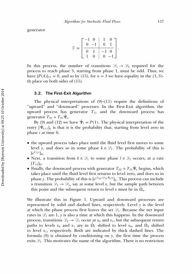
We illustrate this in Figure 1. Upward and downward processes arerepresented by solid and dashed lines, respectively. Level y is the levelat which the phase process first leaves the set �1. Because the net inputrates in �1 are 1, y is also a time at which this happens. In the downwardprocess, transitions �2 → �1 occur at x0 and x1, but the subsequent returnpaths to levels x0 and x1 are in �1 shifted to level x0, and �2 shiftedto level x1, respectively. Both are indicated by thick dashed lines. Theformula (9) is obtained by conditioning on y, the first time the processexits �1. This motivates the name of the algorithm. There is no restriction
Dow
nloa
ded
by [
Rye
rson
Uni
vers
ity]
at 0
9:25
10
Oct
ober
201
4
158 Bean, O’Reilly, and Taylor
FIGURE 1 A path in �3.
on the maximum number of peaks in a sample path contributing to �n forn > 1.
Note that conditioning analogous to the one outlined here wasintroduced in Ref.[9] to derive the formula for � in a simplified fluid flowmodel.
3.3. The Last-Entrance Algorithm
This algorithm is very similar to the First-Exit algorithm. In fact,time reversal in the physical interpretation for the nth iteration of onealgorithm, leads to the physical interpretation of the other. We omit thedetails. The formula (10) is obtained by conditioning on the level y atwhich the process last enters the set �2, motivating the name of thealgorithm. As with the First-Exit algorithm, there is no restriction on themaximum number of peaks in a sample path contributing to �n for n > 1.Conditioning analogous to the one outlined here was introduced in Ref.[21]
to derive the formula for � in a simplified fluid flow model.
Dow
nloa
ded
by [
Rye
rson
Uni
vers
ity]
at 0
9:25
10
Oct
ober
201
4
Algorithms for Stochastic Fluid Flows 159
3.4. Newton's Method
Observe that, with F(Z) = T11Z + ZT22 + ZT21Z + T12, equation (2) canbe written in the form F(�) = 0. Newton’s method is a well-known method(see Ref.[20], for example), which can be used to approximate a solution ofan equation of type F(X) = 0, provided that it exists, with the iteration
Xk+1 = Xk − [F ′(Xk)]−1F(Xk).
In Ref.[13] Guo established the important fact that Newton’s method for thesolution of (2) is equivalent to the iteration (6). This fact has a significantconsequence. In Lemma 1 in Section 3 we show that (11) is equivalentto (6). Consequently, the physical interpretation of algorithm (11) givenbelow is in fact the physical interpretation of Newton’s method[13] in thefluid flow model. This was previously not known.
Newton’s method resembles the First-Exit and Last-Entrancealgorithms in the sense that in a sample path contributing to the (n + 1)-stiteration, exactly as in the two former algorithms, an upward process takesplace, followed by a transition �1 → �2, after which a downward processbegins, which takes place until the fluid level returns to zero. However, inNewton’s method, paths in �n+1 for n ≥ 1 are more complex than paths in�n+1 or �n+1. Observe that, in the First Exit algorithm, only the downwardprocess has a complex structure, while in the Last-Entrance algorithm,only the upward process does. In Newton’s method both upward anddownward processes have a complex structure.
By (11) and (12) we have �1 = P(1). The physical interpretation of�n+1 is that, for i ∈ �1 and j ∈ �2, [�n+1]ij is the probability mass of alldistinct sample paths contributing to [� ]ij in which, starting from level zeroin phase i, for some y ≥ 0,
• first, the upward process takes place. The fluid level moves to somelevel y and does so in some phase k ∈ �1. The probability of this is[e(T11+�nT21)y]ik.
• Next, a transition from k ∈ �1 to some l ∈ �2 occurs, at a rate [T12]kl.• Finally, the downward process takes place, until the fluid returns to level
zero in some phase j ∈ �2. The probability of this is [e(T22+T21�n)y]lj.
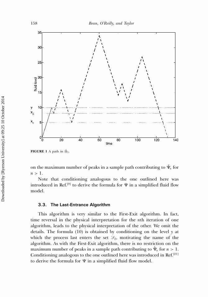
The probability mass of all such paths is the (i, j)-th entry of thematrix (11). We illustrate this in Figure 2. Level y is the level at which theupward process ends and the downward process begins. Observe that levely in general is not the maximum level reached in a sample path. Also notethat the choice of y is not unique as we discuss below. The parts of thesample path, within the upward process, which are indicated by thick solidlines are in �2 shifted to level x0 and �1 shifted to level x2 respectively.
Dow
nloa
ded
by [
Rye
rson
Uni
vers
ity]
at 0
9:25
10
Oct
ober
201
4
160 Bean, O’Reilly, and Taylor
FIGURE 2 A sample path in �3.
The parts of the sample path, within the downward process, which areindicated by thick dashed lines are in �1 shifted to level x3 and �2 shiftedto level x1 respectively.
By conditioning on y, without checking whether the sample paths aredistinct, one might obtain the incorrect formula∫ ∞
0e(T11+�nT21)yT12e(T22+T21�n)y dy. (16)
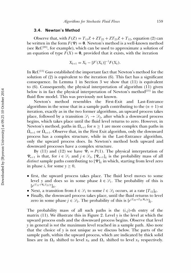
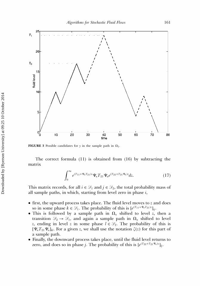
This formula leads to multiple counting of the same sample path. Forexample, consider the sample path in �2 illustrated in Figure 3. In thispath, two possible candidates y0 and y1 for level y are indicated. Eachchoice of y is valid, as for each of them, the upward process and thedownward processes conform to the definitions. To see this, observe thatthe parts indicated by thick solid and dashed lines are all in �1 shiftedto some level. Consequently, this sample path will contribute twice to theintegral (16), for n = 1.
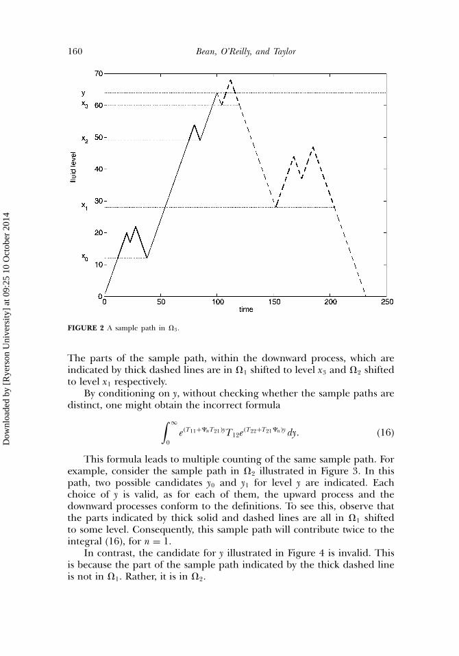
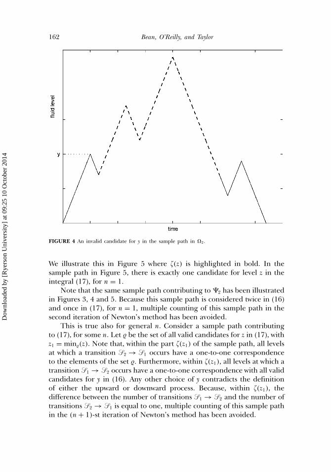
In contrast, the candidate for y illustrated in Figure 4 is invalid. Thisis because the part of the sample path indicated by the thick dashed lineis not in �1. Rather, it is in �2.
Dow
nloa
ded
by [
Rye
rson
Uni
vers
ity]
at 0
9:25
10
Oct
ober
201
4
Algorithms for Stochastic Fluid Flows 161
FIGURE 3 Possible candidates for y in the sample path in �2.
The correct formula (11) is obtained from (16) by subtracting thematrix ∫ ∞
0e(T11+�nT21)z�nT21�ne(T22+T21�n)zdz. (17)
This matrix records, for all i ∈ �1 and j ∈ �2, the total probability mass ofall sample paths, in which, starting from level zero in phase i,
• first, the upward process takes place. The fluid level moves to z and doesso in some phase k ∈ �1. The probability of this is [e(T11+�nT21)z]ij.
• This is followed by a sample path in �n shifted to level z, then atransition �2 → �1, and again a sample path in �n shifted to levelz, ending in level z in some phase l ∈ �2. The probability of this is[�nT21�n]kl. For a given z, we shall use the notation (z) for this part ofa sample path.
• Finally, the downward process takes place, until the fluid level returns tozero, and does so in phase j. The probability of this is [e(T22+T21�n)z]lj.
Dow
nloa
ded
by [
Rye
rson
Uni
vers
ity]
at 0
9:25
10
Oct
ober
201
4
162 Bean, O’Reilly, and Taylor
FIGURE 4 An invalid candidate for y in the sample path in �2.
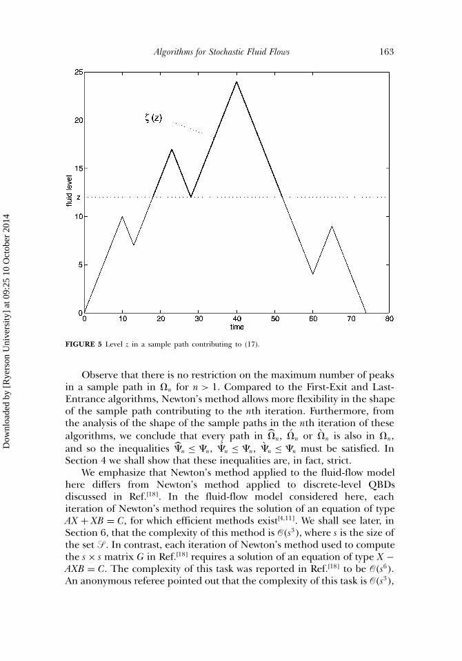
We illustrate this in Figure 5 where (z) is highlighted in bold. In thesample path in Figure 5, there is exactly one candidate for level z in theintegral (17), for n = 1.
Note that the same sample path contributing to �2 has been illustratedin Figures 3, 4 and 5. Because this sample path is considered twice in (16)and once in (17), for n = 1, multiple counting of this sample path in thesecond iteration of Newton’s method has been avoided.
This is true also for general n. Consider a sample path contributingto (17), for some n. Let be the set of all valid candidates for z in (17), withz1 = min(z). Note that, within the part (z1) of the sample path, all levelsat which a transition �2 → �1 occurs have a one-to-one correspondenceto the elements of the set . Furthermore, within (z1), all levels at which atransition �1 → �2 occurs have a one-to-one correspondence with all validcandidates for y in (16). Any other choice of y contradicts the definitionof either the upward or downward process. Because, within (z1), thedifference between the number of transitions �1 → �2 and the number oftransitions �2 → �1 is equal to one, multiple counting of this sample pathin the (n + 1)-st iteration of Newton’s method has been avoided.
Dow
nloa
ded
by [
Rye
rson
Uni
vers
ity]
at 0
9:25
10
Oct
ober
201
4
Algorithms for Stochastic Fluid Flows 163
FIGURE 5 Level z in a sample path contributing to (17).
Observe that there is no restriction on the maximum number of peaksin a sample path in �n for n > 1. Compared to the First-Exit and Last-Entrance algorithms, Newton’s method allows more flexibility in the shapeof the sample path contributing to the nth iteration. Furthermore, fromthe analysis of the shape of the sample paths in the nth iteration of thesealgorithms, we conclude that every path in �n, �n or �n is also in �n,and so the inequalities �n ≤ �n, �n ≤ �n, �n ≤ �n must be satisfied. InSection 4 we shall show that these inequalities are, in fact, strict.
We emphasize that Newton’s method applied to the fluid-flow modelhere differs from Newton’s method applied to discrete-level QBDsdiscussed in Ref.[18]. In the fluid-flow model considered here, eachiteration of Newton’s method requires the solution of an equation of typeAX + XB = C, for which efficient methods exist[4,11]. We shall see later, inSection 6, that the complexity of this method is �(s3), where s is the size ofthe set � . In contrast, each iteration of Newton’s method used to computethe s × s matrix G in Ref.[18] requires a solution of an equation of type X −AXB = C. The complexity of this task was reported in Ref.[18] to be �(s6).An anonymous referee pointed out that the complexity of this task is �(s3),
Dow
nloa
ded
by [
Rye
rson
Uni
vers
ity]
at 0
9:25
10
Oct
ober
201
4
164 Bean, O’Reilly, and Taylor
when using the approach suggested in Ref.[10]. An interesting questionis whether, in the context of approximating the matrix G in the QBDs,it would be more efficient to use Newton’s method[18], implemented asdescribed in Ref.[10], than the Logarithmic Reduction algorithm[19].
3.5. Asmussen's Iteration
The key to the physical interpretation of Asmussen’s iteration(Theorem 3.1[3]) is the first line of the expression for ‘�(−+)
ij ’ on page30 of Ref.[3]. A simplified form of this expression was used to define arecursion for the calculation of �(−+)(n + 1) from �(−+)(n). An analysis ofall possible sample paths in �(−+)(n), leads to the physical interpretationof the scheme. Note that the matrix �(−+) is symmetrical to � in thesense that, in the model which allows for negative fluid levels, �(−+)
ij isthe probability that the process starting from level zero in phase i ∈ �2
first returns to level zero and does so in phase j ∈ �1, while avoidinglevels above zero. For the purpose of comparing this scheme with otheralgorithms, we give this interpretation in terms of � . We shall use thenotation � A
n and �An in a manner analogous to our analysis of other
algorithms.The entry [� A
1 ]ij is the return probability of a journey in which, startingfrom level zero in phase i,
• the phase process remains in phase i, and so the fluid level increasesuntil the transition of the phase process �1 → �2 occurs, at which pointthe fluid level begins to decrease,
• next, the phase process remains in the set �2 until the fluid level firstreaches level zero and does so in phase j.
The entry [� An+1]ij is the return probability of a journey in which,
starting from level zero in phase i, only two options are allowed. The firstoption is that
• the phase process remains in phase i, and so the fluid level increasesuntil the transition of the phase process �1 → �2 occurs, at which pointthe fluid level begins to decrease, and then
• a process with generator T22 + T21�An begins, which takes place until the
fluid level returns to 0 and does so in phase j.
The second option is that
• the phase process remains in phase i, and so the fluid level increases,until the transition of the phase process �1 → �1 occurs, at say level x.
Dow
nloa
ded
by [
Rye
rson
Uni
vers
ity]
at 0
9:25
10
Oct
ober
201
4
Algorithms for Stochastic Fluid Flows 165
• Next, a sample path in �An shifted to level x occurs, and then,
• a process with generator T22 + T21�An begins, which takes place until the
fluid level first returns to 0 and does so in phase j.
In a sample path in �An, in the initial excursion within the set �1, the
phase process is allowed to visit at most n states in �1. In other words,at most (n − 1) transitions �1 → �1 are allowed in the initial excursionwithin set �1. Further, in every subsequent such excursion, at most(n − 1) visits to states in �1 (or (n − 2) transitions �1 → �1) are allowed(per excursion). This means that, an up-slope of every peak in �A
n has avery restricted form because of the restriction on the number of transitionswithin �1. Consequently, this iteration scheme might not be expectedto perform well for processes in which many such transitions occur withhigh probability. In comparison, we have shown earlier that fixed-pointiteration FP3[13], which is restricted in terms of the maximum number ofpeaks in � (n), has total flexibility on the up-slope of every peak. Fromthe analysis of the shape of sample paths in the nth iteration of the First-Exit algorithm and Asmussen’s iteration (Theorem 3.1[3]) we conclude that�A
n ⊆ �n and so � An ≤ �n. A rigorous proof of this fact is given in Section 4.
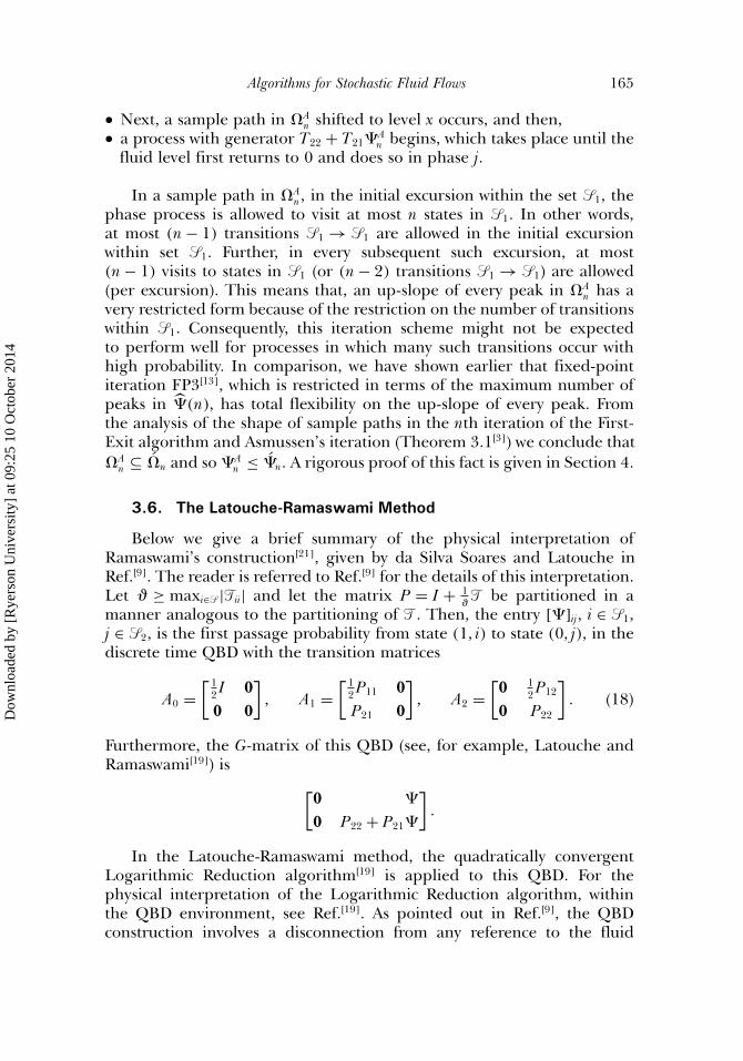
3.6. The Latouche-Ramaswami Method
Below we give a brief summary of the physical interpretation ofRamaswami’s construction[21], given by da Silva Soares and Latouche inRef.[9]. The reader is referred to Ref.[9] for the details of this interpretation.Let � ≥ maxi∈� |�ii| and let the matrix P = I + 1
�� be partitioned in a
manner analogous to the partitioning of � . Then, the entry [� ]ij, i ∈ �1,j ∈ �2, is the first passage probability from state (1, i) to state (0, j), in thediscrete time QBD with the transition matrices
A0 =[ 1
2I 00 0
], A1 =
[ 12P11 0P21 0
], A2 =
[0 1
2P12
0 P22
]. (18)
Furthermore, the G-matrix of this QBD (see, for example, Latouche andRamaswami[19]) is [
0 �
0 P22 + P21�
].
In the Latouche-Ramaswami method, the quadratically convergentLogarithmic Reduction algorithm[19] is applied to this QBD. For thephysical interpretation of the Logarithmic Reduction algorithm, withinthe QBD environment, see Ref.[19]. As pointed out in Ref.[9], the QBDconstruction involves a disconnection from any reference to the fluid
Dow
nloa
ded
by [
Rye
rson
Uni
vers
ity]
at 0
9:25
10
Oct
ober
201
4
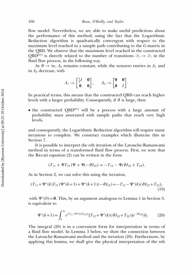
166 Bean, O’Reilly, and Taylor
flow model. Nevertheless, we are able to make useful predictions aboutthe performance of this method, using the fact that the LogarithmicReduction algorithm is quadratically convergent with respect to themaximum level reached in a sample path contributing to the G-matrix inthe QBD. We observe that the maximum level reached in the constructedQBD[21] is directly related to the number of transitions �1 → �1 in thefluid flow process, in the following way.
As � → ∞, A0 remains constant, while the nonzero entries in A1 andin A2 decrease, with
A1 →[ 1
2I 00 0
], A2 →
[0 00 I
].
In practical terms, this means that the constructed QBD can reach higherlevels with a larger probability. Consequently, if � is large, then
• the constructed QBD[21] will be a process with a large amount ofprobability mass associated with sample paths that reach very highlevels,
and consequently, the Logarithmic Reduction algorithm will require manyiterations to complete. We construct examples which illustrate this inSection 7.
It is possible to interpret the nth iteration of the Latouche-Ramaswamimethod in terms of a transformed fluid flow process. First, we note thatthe Riccati equation (2) can be written in the form
(T11 + �T21)� + �(−�I22) = −T12 − �(�I22 + T22).
As in Section 2, we can solve this using the iteration,
(T11 +� ∗(k)T21)�∗(k+1)+� ∗(k+1)(−�I22)=−T12 −� ∗(k)(�I22 +T22),
(19)
with � ∗(0)=0. This, by an argument analogous to Lemma 1 in Section 3,is equivalent to
� ∗(k+1)=∫ ∞
0e(T11+�∗(k)T21)y[T12 +� ∗(k)(�I22 +T22)]e−�I22ydy. (20)
The integral (20) is in a convenient form for interpretation in terms ofa fluid flow model. In Lemma 3 below, we show the connection betweenthe Latouche-Ramaswami method and the iteration (20). Furthermore, byapplying this lemma, we shall give the physical interpretation of the nth
Dow
nloa
ded
by [
Rye
rson
Uni
vers
ity]
at 0
9:25
10
Oct
ober
201
4
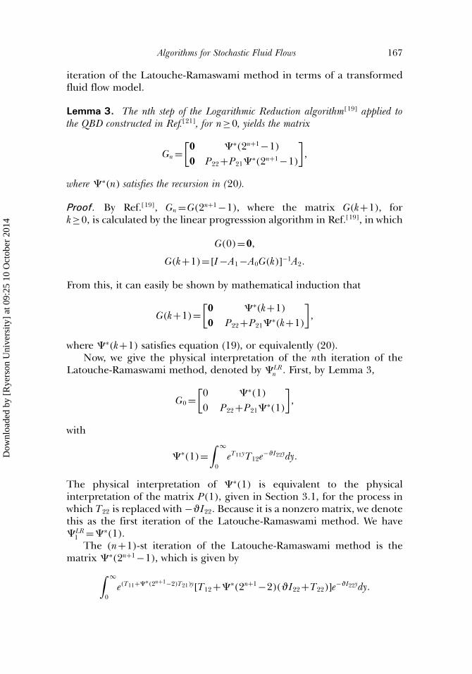
Algorithms for Stochastic Fluid Flows 167
iteration of the Latouche-Ramaswami method in terms of a transformedfluid flow model.
Lemma 3. The nth step of the Logarithmic Reduction algorithm[19] applied tothe QBD constructed in Ref.[21], for n≥0, yields the matrix
Gn =[0 � ∗(2n+1 −1)0 P22 +P21�
∗(2n+1 −1)
],
where � ∗(n) satisfies the recursion in (20).
Proof. By Ref.[19], Gn =G(2n+1 −1), where the matrix G(k+1), fork≥0, is calculated by the linear progresssion algorithm in Ref.[19], in which
G(0)=0,
G(k+1)=[I−A1 −A0G(k)]−1A2.
From this, it can easily be shown by mathematical induction that
G(k+1)=[0 � ∗(k+1)0 P22 +P21�
∗(k+1)
],
where � ∗(k+1) satisfies equation (19), or equivalently (20).Now, we give the physical interpretation of the nth iteration of the
Latouche-Ramaswami method, denoted by � LRn . First, by Lemma 3,
G0 =[0 � ∗(1)0 P22 +P21�
∗(1)
],
with
� ∗(1)=∫ ∞
0eT11yT12e−�I22ydy.
The physical interpretation of � ∗(1) is equivalent to the physicalinterpretation of the matrix P(1), given in Section 3.1, for the process inwhich T22 is replaced with −�I22. Because it is a nonzero matrix, we denotethis as the first iteration of the Latouche-Ramaswami method. We have� LR
1 =� ∗(1).The (n+1)-st iteration of the Latouche-Ramaswami method is the
matrix � ∗(2n+1 −1), which is given by∫ ∞
0e(T11+�∗(2n+1−2)T21)y[T12 +� ∗(2n+1 −2)(�I22 +T22)]e−�I22ydy.
Dow
nloa
ded
by [
Rye
rson
Uni
vers
ity]
at 0
9:25
10
Oct
ober
201
4
168 Bean, O’Reilly, and Taylor
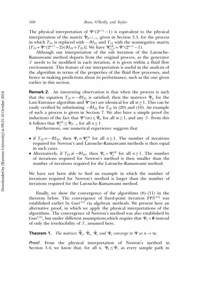
The physical interpretation of � ∗(2n+1 −1) is equivalent to the physicalinterpretation of the matrix �2n+1−1, given in Section 3.3, for the processin which T22 is replaced with −�I22 and T12 with the nonnegative matrix[T12 +� ∗(2n+1 −2)(�I22 +T22)]. We have � LR
n+1 =� ∗(2n+1 −1).Although our interpretation of the nth iteration of the Latouche-
Ramaswami method departs from the original process, as the generator� needs to be modified in each iteration, it is given within a fluid flowenvironment. This feature of our interpretation is useful in the analysis ofthe algorithm in terms of the properties of the fluid flow processes, andhence in making predictions about its performance, such as the one givenearlier in this section.
Remark 2. An interesting observation is that when the process is suchthat the equation T22 =−�I22 is satisfied, then the matrices �m for theLast-Entrance algorithm and � ∗(m) are identical for all m≥1. This can beeasily verified by substituting −�I22 for T22 in (20) and (10). An exampleof such a process is given in Section 7. We also have a simple proof (byinduction) of the fact that � ∗(m)≤�m for all m≥1, and any � . From thisit follows that � LR
n ≤�2n−1 for all n≥1.Furthermore, our numerical experience suggests that
• if T22 =−�I22, then �n =� LRn for all n≥1. The number of iterations
required for Newton’s and Latouche-Ramaswami methods is then equalin such cases.
• Alternatively, if T22 �=−�I22, then �n>� LRn for all n≥1. The number
of iterations required for Newton’s method is then smaller than thenumber of iterations required for the Latouche-Ramaswami method.
We have not been able to find an example in which the number ofiterations required for Newton’s method is larger than the number ofiterations required for the Latouche-Ramaswami method.
Finally, we show the convergence of the algorithms (8)–(11) in thetheorem below. The convergence of fixed-point iteration FP3[13] wasestablished earlier by Guo[13] via algebraic methods. We present here analternative proof, in which we apply the physical interpretations of thealgorithms. The convergence of Newton’s method was also established byGuo[13], but under different assumptions,which require that �1>0 insteadof only the irreducibility of � , assumed here.
Theorem 1. The matrices �n, �n, �n and �n converge to � as n→∞.
Proof. From the physical interpretation of Newton’s method inSection 3.4, we know that, for all n, �n ≤� , as every sample path in
Dow
nloa
ded
by [
Rye
rson
Uni
vers
ity]
at 0
9:25
10
Oct
ober
201
4
Algorithms for Stochastic Fluid Flows 169
�n contributes to � . Furthermore, by Section 3.4, every sample pathcontributing to � lies in �n for some n. Hence, the convergence ofNewton’s method follows. The proof of the remaining results is analogous.
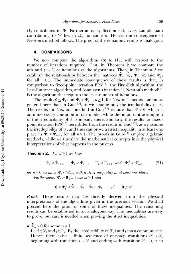
4. COMPARISONS
We now compare the algorithms (8) to (11) with respect to thenumber of iterations required. First, in Theorem 2 we compare thenth and (n+1)-st iterations of the algorithms. Then, in Theorem 3 weestablish the relationships between the matrices �n, �n, �n, �n and � A
n ,for all n≥1. The immediate consequence of these results is that, incomparison to fixed-point iteration FP3[13], the First-Exit algorithm, theLast-Entrance algorithm, and Asmussen’s iteration[3], Newton’s method[13]
is the algorithm that requires the least number of iterations.The results 0≤�1 and �n<�n+1, n≥1, for Newton’s method, are more
general here than in Guo[13], as we assume only the irreducibility of � .The results for Newton’s method in Guo[13] require that �1>0, which isan unnecessary condition in our model, while the important assumptionof the irreducibility of � is missing there. Similarly, the results for fixed-point iteration FP3[13] here differ from the results in Guo[13], as we assumethe irreducibility of � , and thus can prove a strict inequality in at least oneplace in �n ≤�n+1, for all n≥1. The proofs in Guo[13] employ algebraicmethods, while we translate the mathematical concepts into the physicalinterpretations of what happens in the process.
Theorem 2. For n≥1 we have
�n<�n+1, �n<�n+1, �n<�n+1 and � An <� A
n+1, (21)
for n≥0 we have �n ≤�n+1 with a strict inequality in at least one place.Furthermore, �m>0 for some m≥1 and
0≤� A1 ≤�1 =�1 =�1 =�1 with 0 �=� A
1 .
Proof. These results may be directly derived from the physicalinterpretations of the algorithms given in the previous section. We shallpresent here the proof of some of these inequalities. The remainingresults can be established in an analogous way. The inequalities are easyto prove, but care is needed when proving the strict inequalities.
• �m>0 for some m≥1.Let i∈�1 and j∈�2. By the irreducibility of � , i and j must communicate.Hence, there exists a finite sequence of one-step transitions � →� ,beginning with transition i→� and ending with transition � → j, such
Dow
nloa
ded
by [
Rye
rson
Uni
vers
ity]
at 0
9:25
10
Oct
ober
201
4
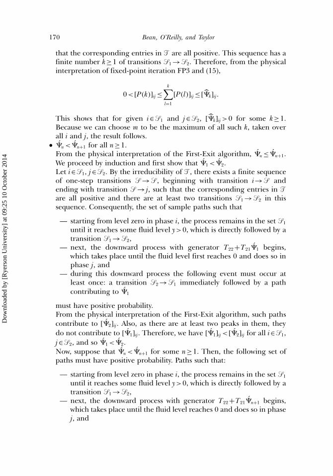
170 Bean, O’Reilly, and Taylor
that the corresponding entries in � are all positive. This sequence has afinite number k≥1 of transitions �1 →�2. Therefore, from the physicalinterpretation of fixed-point iteration FP3 and (15),
0< [P(k)]ij ≤k∑
l=1
[P(l)]ij ≤[�k]ij.
This shows that for given i∈�1 and j∈�2, [�k]ij >0 for some k≥1.Because we can choose m to be the maximum of all such k, taken overall i and j, the result follows.
• �n<�n+1 for all n≥1.From the physical interpretation of the First-Exit algorithm, �n ≤�n+1.We proceed by induction and first show that �1<�2.Let i∈�1, j∈�2. By the irreducibility of � , there exists a finite sequenceof one-step transitions � →� , beginning with transition i→� andending with transition � → j, such that the corresponding entries in �are all positive and there are at least two transitions �1 →�2 in thissequence. Consequently, the set of sample paths such that
— starting from level zero in phase i, the process remains in the set �1
until it reaches some fluid level y>0, which is directly followed by atransition �1 →�2,
— next, the downward process with generator T22 +T21�1 begins,which takes place until the fluid level first reaches 0 and does so inphase j, and
— during this downward process the following event must occur atleast once: a transition �2 →�1 immediately followed by a pathcontributing to �1
must have positive probability.From the physical interpretation of the First-Exit algorithm, such pathscontribute to [�2]ij. Also, as there are at least two peaks in them, theydo not contribute to [�1]ij. Therefore, we have [�1]ij < [�2]ij for all i∈�1,j∈�2, and so �1<�2.Now, suppose that �n<�n+1 for some n≥1. Then, the following set ofpaths must have positive probability. Paths such that:
— starting from level zero in phase i, the process remains in the set �1
until it reaches some fluid level y>0, which is directly followed by atransition �1 →�2,
— next, the downward process with generator T22 +T21�n+1 begins,which takes place until the fluid level reaches 0 and does so in phasej, and
Dow
nloa
ded
by [
Rye
rson
Uni
vers
ity]
at 0
9:25
10
Oct
ober
201
4
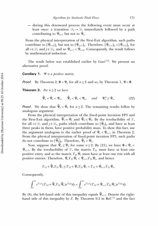
Algorithms for Stochastic Fluid Flows 171
— during this downward process the following event must occur atleast once: a transition �2 →�1 immediately followed by a pathcontributing to �n+1 but not to �n.
From the physical interpretation of the First-Exit algorithm, such pathscontribute to [�n+2]ij but not to [�n+1]ij. Therefore, [�n+1]ij < [�n+2]ij forall i∈�1 and j∈�2, and so �n+1<�n+2. Consequently, the result followsby mathematical induction.
The result below was established earlier by Guo[14]. We present analternative proof.
Corollary 1. � is a positive matrix.
Proof. By Theorem 2, 0<�n for all n≥2 and so, by Theorem 1, �>0.
Theorem 3. For n≥2 we have
�n<�n<�n, �n<�n<�n, and � An ≤�n. (22)
Proof. We show that �n<�n for n≥2. The remaining results follow byanalogous argument.
From the physical interpretation of the fixed-point iteration FP3 andthe First-Exit algorithm, �1 =�1 and �2 ≤�2. By the irreducibility of � ,for all i∈�1 and j∈�2, paths which contribute to [�2]ij and have at leastthree peaks in them, have positive probability mass. To show this fact, usethe argument analogous to the earlier proof of �n<�n+1 in Theorem 2.From the physical interpretation of fixed-point iteration FP3, such pathsdo not contribute to [�2]ij. Therefore, �2<�2.
Now, suppose that �n ≤�n for some n≥2. By (21), we have 0<�n<
�n+1. By the irreducibility of � , the matrix T21 must have at least onepositive entry, and so the matrix T21�n must have at least one row with allpositive entries. Therefore, �nT21�n<�n+1T21�n, and hence
T12 +�nT21�n ≤T12 +�nT21�n<T12 +�n+1T21�n.
Consequently,∫ ∞
0eT11y(T12 +�nT21�n)eT22ydy<
∫ ∞
0eT11y(T12 +�n+1T21�n)eT22ydy.
By (8), the left-hand side of this inequality equals �n+1. Denote the right-hand side of this inequality by Z. By Theorem 9.2 in Ref.[7] and the fact
Dow
nloa
ded
by [
Rye
rson
Uni
vers
ity]
at 0
9:25
10
Oct
ober
201
4
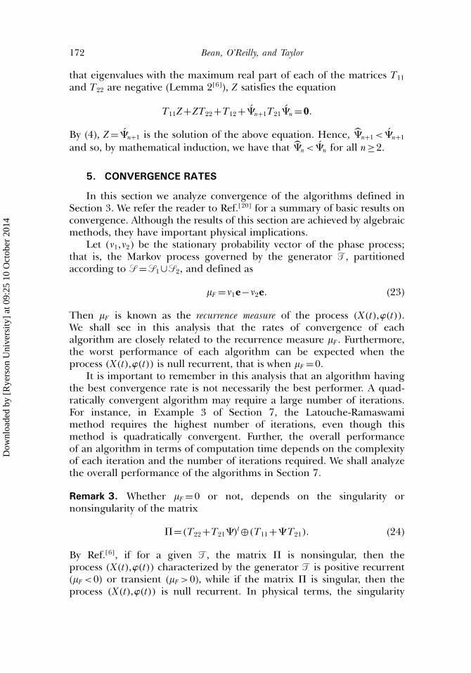
172 Bean, O’Reilly, and Taylor
that eigenvalues with the maximum real part of each of the matrices T11
and T22 are negative (Lemma 2[6]), Z satisfies the equation
T11Z+ZT22 +T12 +�n+1T21�n =0.
By (4), Z=�n+1 is the solution of the above equation. Hence, �n+1<�n+1
and so, by mathematical induction, we have that �n<�n for all n≥2.
5. CONVERGENCE RATES
In this section we analyze convergence of the algorithms defined inSection 3. We refer the reader to Ref.[20] for a summary of basic results onconvergence. Although the results of this section are achieved by algebraicmethods, they have important physical implications.
Let ( 1, 2) be the stationary probability vector of the phase process;that is, the Markov process governed by the generator � , partitionedaccording to � =�1 ∪�2, and defined as
�F = 1e− 2e. (23)
Then �F is known as the recurrence measure of the process (X(t),�(t)).We shall see in this analysis that the rates of convergence of eachalgorithm are closely related to the recurrence measure �F . Furthermore,the worst performance of each algorithm can be expected when theprocess (X(t),�(t)) is null recurrent, that is when �F =0.
It is important to remember in this analysis that an algorithm havingthe best convergence rate is not necessarily the best performer. A quad-ratically convergent algorithm may require a large number of iterations.For instance, in Example 3 of Section 7, the Latouche-Ramaswamimethod requires the highest number of iterations, even though thismethod is quadratically convergent. Further, the overall performanceof an algorithm in terms of computation time depends on the complexityof each iteration and the number of iterations required. We shall analyzethe overall performance of the algorithms in Section 7.
Remark 3. Whether �F =0 or not, depends on the singularity ornonsingularity of the matrix
�=(T22 +T21�)t ⊕(T11 +�T21). (24)
By Ref.[6], if for a given � , the matrix � is nonsingular, then theprocess (X(t),�(t)) characterized by the generator � is positive recurrent(�F <0) or transient (�F >0), while if the matrix � is singular, then theprocess (X(t),�(t)) is null recurrent. In physical terms, the singularity
Dow
nloa
ded
by [
Rye
rson
Uni
vers
ity]
at 0
9:25
10
Oct
ober
201
4
Algorithms for Stochastic Fluid Flows 173
or nonsingularity of the matrix � can be explained in the followingway. Consider two processes (X1,�(t)) and (X2,�(t)) with generators U1 =(T11 +�T21) and U2 =(T22 +T21�) respectively. If both these processes arerecurrent, then by Ref.[22] the matrices U1 and U2 both have 0 as theirdominant eigenvalue. Hence, by Ref.[12] the matrix � is singular, whichin turn implies the null recurrence of the fluid flow process (X(t),�(t)).Alternatively, by Refs.[12,22], if one of the processes is recurrent and theother transient, then the matrix � is nonsingular. In summary
• if both (X1,�(t)) and (X2,�(t)) are recurrent, then the fluid flow process(X(t),�(t)) is null recurrent,
• if the process (X1,�(t)) is transient and (X2,�(t)) is recurrent, then thefluid flow process (X(t),�(t)) is positive recurrent, while
• if the process (X1,�(t)) is recurrent and (X2,�(t)) is transient, then thefluid flow process (X(t),�(t)) is transient.
Let us recall a few basic concepts from Ref.[20], which we will needin this analysis. First, we define a measure of the rate of convergence ofiterative processes. Let p≥1. Then, an R-factor for p of the sequence �Ak�
converging to A, as k→∞, is
Rp�Ak�={
lim supk→∞‖Ak −A‖1/k if p=1,lim supk→∞‖Ak −A‖1/pk if p>1.
(25)
Now, if 0<R1�Ak�<1, then we say that the convergence is R-linear, whileif R1�Ak�=1 or R1�Ak�=0, then the convergence is R-sublinear or R-superlinear, respectively. If 0<R2�Ak�<1, then the convergence is R-quadratic. When R1�Ak�>0, R-quadratic convergence is not possible.
Let R1 be the R-factor for 1[20] of fixed-point iteration FP3[13], thatis R1 = lim supn→∞(‖�n −�‖) 1
n . Similarly, let R1, R1, RA1, R1 and RLR
1
be the R-factors for 1 of the First-Exit algorithm, the Last-Entrancealgorithm, Asmussen’s iteration[3], Newton’s method[13] and the Latouche-Ramaswami method, respectively.
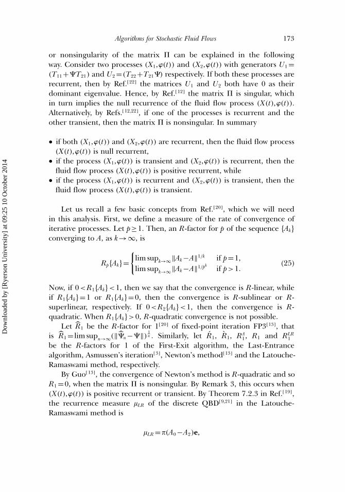
By Guo[13], the convergence of Newton’s method is R-quadratic and soR1 =0, when the matrix � is nonsingular. By Remark 3, this occurs when(X(t),�(t)) is positive recurrent or transient. By Theorem 7.2.3 in Ref.[19],the recurrence measure �LR of the discrete QBD[9,21] in the Latouche-Ramaswami method is
�LR =�(A0 −A2)e,
Dow
nloa
ded
by [
Rye
rson
Uni
vers
ity]
at 0
9:25
10
Oct
ober
201
4
174 Bean, O’Reilly, and Taylor
where � is the stationary probability vector of the Markov process withgenerator Q =A0 +A1 +A2, with A0, A1, A2 given by (18). It is easy to showthat
�LR =�F/(1+ 1e). (26)
Consequently, by Ref.[15], the convergence of the Logarithmic Reductionalgorithm applied in the Latouche-Ramaswami method is also R-quadraticand RLR
1 =0, when the process (X(t),�(t)) is positive recurrent or transient.Note however that, when the process (X(t),�(t)) is null recurrent (and sothe QBD is also null recurrent), the convergence may be linear. Guo[13,15]
conjectured that when the QBD is null recurrent, the convergence of bothNewton’s method and the Latouche-Ramaswami method is R-linear withR-factor equal to 1/2.
Theorem 4 below determines the convergence of the First-Exitalgorithm, the Last-Entrance algorithm and Asmussen’s iteration[3]. Forcompleteness, we have included Guo’s result for fixed-point iterationFP3[13]. We have added our proof of the fact that R1 is a positivenumber, which was not shown in Ref.[13]. This fact confirms that neitherR-superlinear nor R-quadratic convergence is possible. The consequenceof this theorem is that, when the process (X(t),�(t)) is positive recurrent ortransient, then the convergence of fixed-point iteration FP3[13], the First-Exit algorithm, the Last-Entrance algorithm and Asmussen’s iteration[3]
is R-linear, while when the process (X(t),�(t)) is null recurrent, then thisconvergence is R-sublinear.
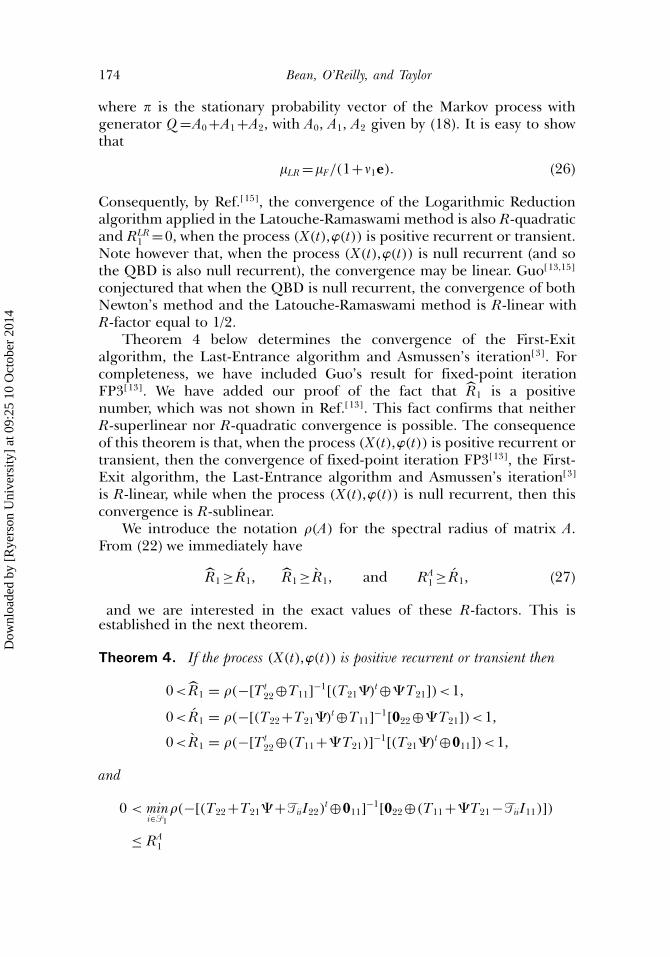
We introduce the notation �(A) for the spectral radius of matrix A.From (22) we immediately have
R1 ≥ R1, R1 ≥ R1, and RA1 ≥ R1, (27)
and we are interested in the exact values of these R-factors. This isestablished in the next theorem.
Theorem 4. If the process (X(t),�(t)) is positive recurrent or transient then
0< R1 = �(−[Tt22 ⊕T11]−1[(T21�)t ⊕�T21])<1,
0< R1 = �(−[(T22 +T21�)t ⊕T11]−1[022 ⊕�T21])<1,
0< R1 = �(−[Tt22 ⊕(T11 +�T21)]−1[(T21�)t ⊕011])<1,
and
0 < mini∈�1
�(−[(T22 +T21�+�iiI22)t ⊕011]−1[022 ⊕(T11 +�T21 −�iiI11)])
≤ RA1
Dow
nloa
ded
by [
Rye
rson
Uni
vers
ity]
at 0
9:25
10
Oct
ober
201
4
Algorithms for Stochastic Fluid Flows 175
≤ maxi∈�1
�(−[(T22 +T21�+�iiI22)t ⊕011]−1[022 ⊕(T11 +�T21 −�iiI11)])
< 1.
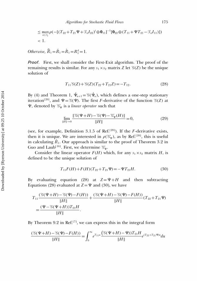
Otherwise, R1 = R1 = R1 =RA1 =1.
Proof. First, we shall consider the First-Exit algorithm. The proof of theremaining results is similar. For any s1 ×s2 matrix Z let �(Z) be the uniquesolution of
T11�(Z)+�(Z)(T22 +T21Z)=−T12. (28)
By (4) and Theorem 1, �n+1 =�(�n), which defines a one-step stationaryiteration[20], and � =�(�). The first F-derivative of the function �(Z) at� , denoted by �′
� is a linear operator such that
lim‖H‖→0
‖�(�+H)−�(�)−�′�(H)‖
‖H‖ =0, (29)
(see, for example, Definition 3.1.5 of Ref.[20]). If the F-derivative exists,then it is unique. We are interested in �(�′
�), as by Ref.[20], this is usefulin calculating R1. Our approach is similar to the proof of Theorem 3.2 inGuo and Laub[16]. First, we determine �′
� .Consider the linear operator F(H) which, for any s1 ×s2 matrix H, is
defined to be the unique solution of
T11F(H)+F(H)(T22 +T21�)=−�T21H. (30)
By evaluating equation (28) at Z=�+H and then subtractingEquations (28) evaluated at Z=� and (30), we have
T11(�(�+H)−�(�)−F(H))
‖H‖ + (�(�+H)−�(�)−F(H))
‖H‖ (T22 +T21�)
= (�−�(�+H))T21H‖H‖ .
By Theorem 9.2 in Ref.[7], we can express this in the integral form
(�(�+H)−�(�)−F(H))
‖H‖ =∫ ∞
0eT11u
(�(�+H)−�))T21H
‖H‖ e(T22+T21�)udu
Dow
nloa
ded
by [
Rye
rson
Uni
vers
ity]
at 0
9:25
10
Oct
ober
201
4
176 Bean, O’Reilly, and Taylor
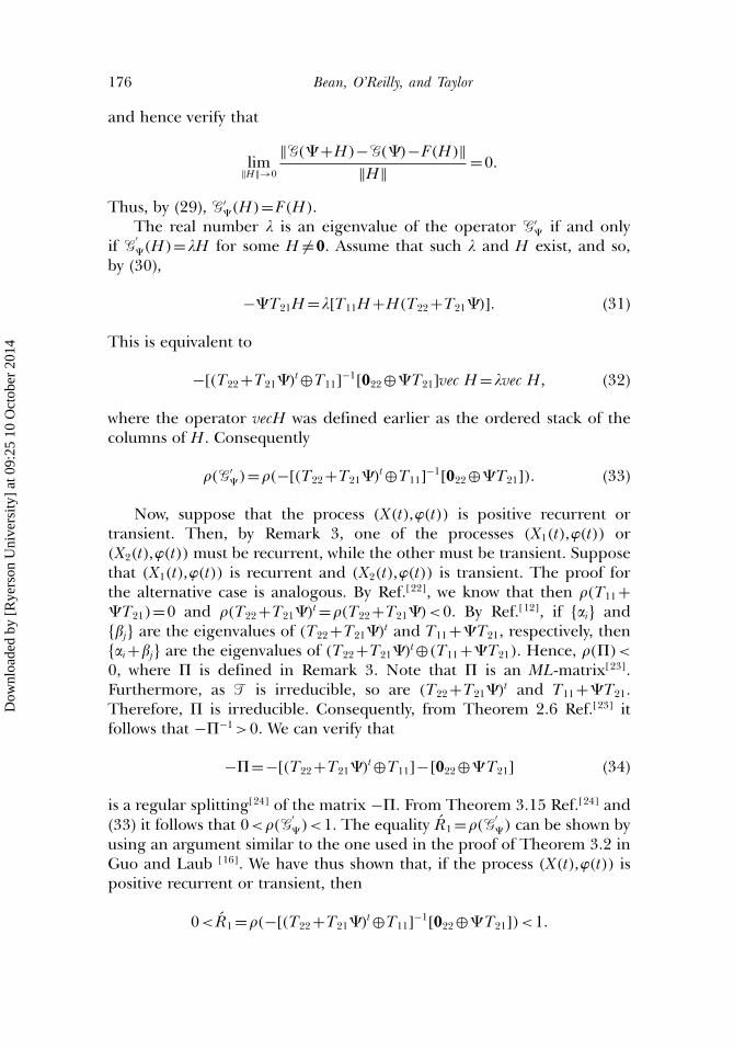
and hence verify that
lim‖H‖→0
‖�(�+H)−�(�)−F(H)‖‖H‖ =0.
Thus, by (29), �′�(H)=F(H).
The real number � is an eigenvalue of the operator �′� if and only
if �′�(H)=�H for some H �=0. Assume that such � and H exist, and so,
by (30),
−�T21H =�[T11H+H(T22 +T21�)]. (31)
This is equivalent to
−[(T22 +T21�)t ⊕T11]−1[022 ⊕�T21]vec H =�vec H, (32)
where the operator vecH was defined earlier as the ordered stack of thecolumns of H. Consequently
�(�′�)=�(−[(T22 +T21�)t ⊕T11]−1[022 ⊕�T21]). (33)
Now, suppose that the process (X(t),�(t)) is positive recurrent ortransient. Then, by Remark 3, one of the processes (X1(t),�(t)) or(X2(t),�(t)) must be recurrent, while the other must be transient. Supposethat (X1(t),�(t)) is recurrent and (X2(t),�(t)) is transient. The proof forthe alternative case is analogous. By Ref.[22], we know that then �(T11 +�T21)=0 and �(T22 +T21�)t =�(T22 +T21�)<0. By Ref.[12], if ��i� and��j� are the eigenvalues of (T22 +T21�)t and T11 +�T21, respectively, then��i +�j� are the eigenvalues of (T22 +T21�)t ⊕(T11 +�T21). Hence, �(�)<0, where � is defined in Remark 3. Note that � is an ML-matrix[23].Furthermore, as � is irreducible, so are (T22 +T21�)t and T11 +�T21.Therefore, � is irreducible. Consequently, from Theorem 2.6 Ref.[23] itfollows that −�−1>0. We can verify that
−�=−[(T22 +T21�)t ⊕T11]−[022 ⊕�T21] (34)
is a regular splitting[24] of the matrix −�. From Theorem 3.15 Ref.[24] and(33) it follows that 0<�(�
′�)<1. The equality R1 =�(�
′�) can be shown by
using an argument similar to the one used in the proof of Theorem 3.2 inGuo and Laub [16]. We have thus shown that, if the process (X(t),�(t)) ispositive recurrent or transient, then
0< R1 =�(−[(T22 +T21�)t ⊕T11]−1[022 ⊕�T21])<1.
Dow
nloa
ded
by [
Rye
rson
Uni
vers
ity]
at 0
9:25
10
Oct
ober
201
4
Algorithms for Stochastic Fluid Flows 177
Alternatively, suppose that the process (X(t),�(t)) is null recurrent.Then, by Remark 3 the matrix � is singular, and so �vecH =0 for someH �=0. By (34),
0=�vec H =−[(T22 +T21�)t ⊕T11]vec H−[022 ⊕�T21]vec H.
Consequently,
−[(T22 +T21�)t ⊕T11]−1[022 ⊕�T21]vec H =vec H,
and hence, by (32), we have �(�′�)=1. Finally, to see that R1 =�(�
′�),
in the null-recurrent case, modify the generator � by putting T(k)12 =
[(k+1)/k]T12, k≥1, so that the new process (X(k)(t),�(k)(t)) is positiverecurrent. Next, repeat the argument for the positive recurrent process(X(k)(t),�(k)(t)) and then take the limit as k→∞. This completes the proofof the result for the First-Exit algorithm. Because we have shown thatR1>0, by (27) it follows that R1>0 and RA
1 >0.
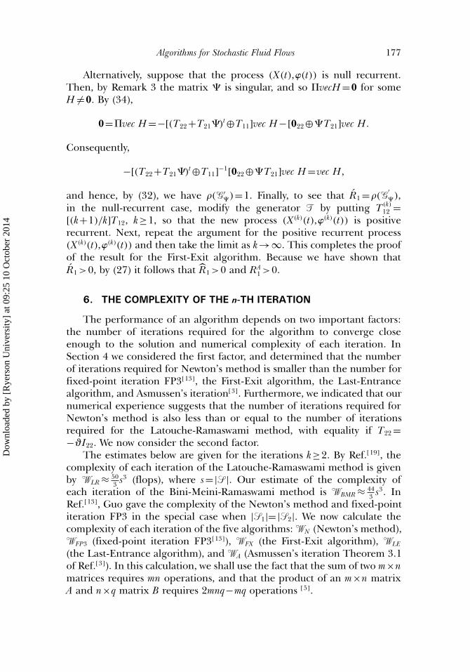
6. THE COMPLEXITY OF THE n-TH ITERATION
The performance of an algorithm depends on two important factors:the number of iterations required for the algorithm to converge closeenough to the solution and numerical complexity of each iteration. InSection 4 we considered the first factor, and determined that the numberof iterations required for Newton’s method is smaller than the number forfixed-point iteration FP3[13], the First-Exit algorithm, the Last-Entrancealgorithm, and Asmussen’s iteration[3]. Furthermore, we indicated that ournumerical experience suggests that the number of iterations required forNewton’s method is also less than or equal to the number of iterationsrequired for the Latouche-Ramaswami method, with equality if T22 =−�I22. We now consider the second factor.
The estimates below are given for the iterations k≥2. By Ref.[19], thecomplexity of each iteration of the Latouche-Ramaswami method is givenby �LR ≈ 50
3 s3 (flops), where s=|� |. Our estimate of the complexity ofeach iteration of the Bini-Meini-Ramaswami method is �BMR ≈ 44
3 s3. InRef.[13], Guo gave the complexity of the Newton’s method and fixed-pointiteration FP3 in the special case when |�1|=|�2|. We now calculate thecomplexity of each iteration of the five algorithms: �N (Newton’s method),�FP3 (fixed-point iteration FP3[13]), �FX (the First-Exit algorithm), �LE
(the Last-Entrance algorithm), and �A (Asmussen’s iteration Theorem 3.1of Ref.[3]). In this calculation, we shall use the fact that the sum of two m×nmatrices requires mn operations, and that the product of an m×n matrixA and n×q matrix B requires 2mnq−mq operations [5].
Dow
nloa
ded
by [
Rye
rson
Uni
vers
ity]
at 0
9:25
10
Oct
ober
201
4
178 Bean, O’Reilly, and Taylor
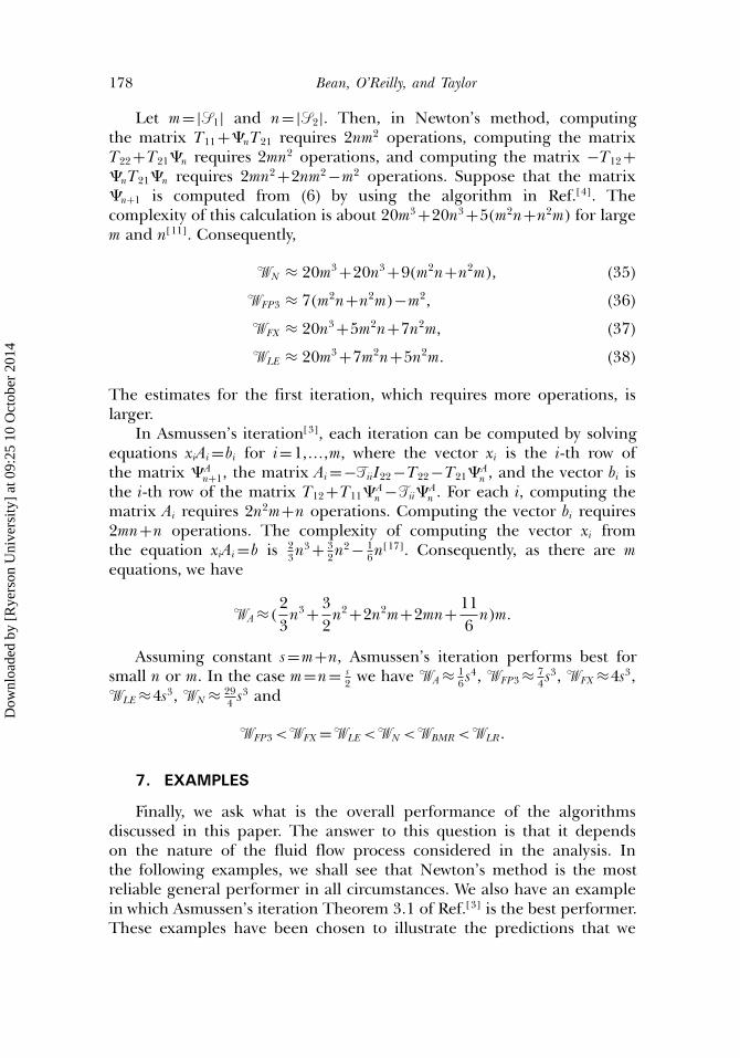
Let m=|�1| and n=|�2|. Then, in Newton’s method, computingthe matrix T11 +�nT21 requires 2nm2 operations, computing the matrixT22 +T21�n requires 2mn2 operations, and computing the matrix −T12 +�nT21�n requires 2mn2 +2nm2 −m2 operations. Suppose that the matrix�n+1 is computed from (6) by using the algorithm in Ref.[4]. Thecomplexity of this calculation is about 20m3 +20n3 +5(m2n+n2m) for largem and n[11]. Consequently,
�N ≈ 20m3 +20n3 +9(m2n+n2m), (35)
�FP3 ≈ 7(m2n+n2m)−m2, (36)
�FX ≈ 20n3 +5m2n+7n2m, (37)
�LE ≈ 20m3 +7m2n+5n2m. (38)
The estimates for the first iteration, which requires more operations, islarger.
In Asmussen’s iteration[3], each iteration can be computed by solvingequations xiAi =bi for i=1,���,m, where the vector xi is the i-th row ofthe matrix � A
n+1, the matrix Ai =−�iiI22 −T22 −T21�An , and the vector bi is
the i-th row of the matrix T12 +T11�An −�ii�
An . For each i, computing the
matrix Ai requires 2n2m+n operations. Computing the vector bi requires2mn+n operations. The complexity of computing the vector xi fromthe equation xiAi =b is 2
3n3 + 32n2 − 1
6n[17]. Consequently, as there are mequations, we have
�A ≈(23
n3 + 32
n2 +2n2m+2mn+ 116
n)m.
Assuming constant s=m+n, Asmussen’s iteration performs best forsmall n or m. In the case m=n= s
2 we have �A ≈ 16 s4, �FP3 ≈ 7
4 s3, �FX ≈4s3,�LE ≈4s3, �N ≈ 29
4 s3 and
�FP3<�FX =�LE<�N <�BMR<�LR.
7. EXAMPLES
Finally, we ask what is the overall performance of the algorithmsdiscussed in this paper. The answer to this question is that it dependson the nature of the fluid flow process considered in the analysis. Inthe following examples, we shall see that Newton’s method is the mostreliable general performer in all circumstances. We also have an examplein which Asmussen’s iteration Theorem 3.1 of Ref.[3] is the best performer.These examples have been chosen to illustrate the predictions that we
Dow
nloa
ded
by [
Rye
rson
Uni
vers
ity]
at 0
9:25
10
Oct
ober
201
4
Algorithms for Stochastic Fluid Flows 179
made based on the physical interpretations of the algorithms in Section 3.All examples are indicative of the expected performance of the algorithmsin similar situations.
We shall use the uniform notation �(n) for the matrix obtained in then-th step. For positive recurrent or null recurrent processes, the inequality
‖e−�(n)e‖∞ ≤�×e
is used as the stopping criterion with �=1e−05 in all such examples. Fortransient processes, we use the inequality
‖�(n+1)e−�(n)e‖∞ ≤�×e
as the stopping criterion, with �=1e−09.We have implemented all the algorithms in MATLAB. Average
CPU times were obtained by running each algorithm 100 times, unlessindicated otherwise. We caution against paying too much attentionto these CPU times, because the algorithms are likely to have beendifferentially affected by the inherent optimization features of MATLAB.To give a fair comparison, each of the algorithms would have to beimplemented in comparable code.
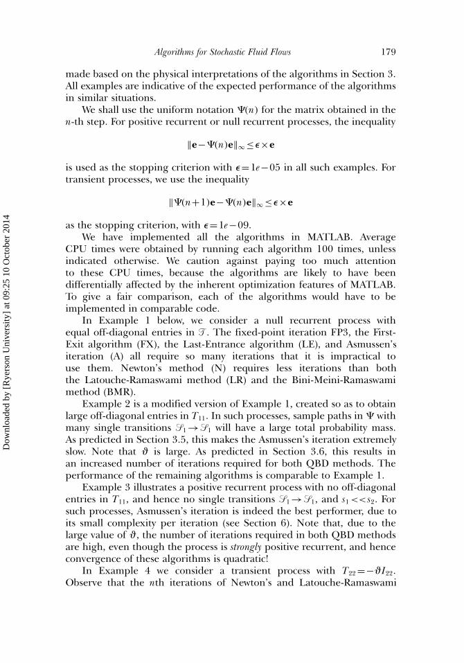
In Example 1 below, we consider a null recurrent process withequal off-diagonal entries in � . The fixed-point iteration FP3, the First-Exit algorithm (FX), the Last-Entrance algorithm (LE), and Asmussen’siteration (A) all require so many iterations that it is impractical touse them. Newton’s method (N) requires less iterations than boththe Latouche-Ramaswami method (LR) and the Bini-Meini-Ramaswamimethod (BMR).
Example 2 is a modified version of Example 1, created so as to obtainlarge off-diagonal entries in T11. In such processes, sample paths in � withmany single transitions �1 →�1 will have a large total probability mass.As predicted in Section 3.5, this makes the Asmussen’s iteration extremelyslow. Note that � is large. As predicted in Section 3.6, this results inan increased number of iterations required for both QBD methods. Theperformance of the remaining algorithms is comparable to Example 1.
Example 3 illustrates a positive recurrent process with no off-diagonalentries in T11, and hence no single transitions �1 →�1, and s1<< s2. Forsuch processes, Asmussen’s iteration is indeed the best performer, due toits small complexity per iteration (see Section 6). Note that, due to thelarge value of �, the number of iterations required in both QBD methodsare high, even though the process is strongly positive recurrent, and henceconvergence of these algorithms is quadratic!
In Example 4 we consider a transient process with T22 =−�I22.Observe that the nth iterations of Newton’s and Latouche-Ramaswami
Dow
nloa
ded
by [
Rye
rson
Uni
vers
ity]
at 0
9:25
10
Oct
ober
201
4

180 Bean, O’Reilly, and Taylor
methods are equal, and hence the number of iterations required forboth methods is the same. We note that in all our numerical experience,whenever T22 =−�I22, the number of iterations in Newton’s method wasequal to the number of iterations in the Latouche-Ramaswami method, andsmaller than the latter, otherwise.
In the tables below, an asterisk next to a method indicates that thealgorithm did not converge in the given number of iterations.
Example 1. Consider the null recurrent process with generator
� =
−0.003 0.001 0.001 0.001
0.001 −0.003 0.001 0.001
0.001 0.001 −0.003 0.0010.001 0.001 0.001 −0.003
.
The outcome of using the various algorithms is shown in Table 1.Note that, by Section 6, the total complexity (including all the
iterations) of Newton’s method for this example is about eight timessmaller than the total complexity of the Bini-Meini-Ramaswami methodand about ten times smaller than the total complexity of the Latouche-Ramaswami method. Theoretically, Newton’s method should performmuch better than both QBD methods. However, this theoretical advantageis not reflected in the average CPU time observed in this example. In fact,the average CPU time is higher for Newton’s method than for the twoother methods. As mentioned above, we conjecture that this is becausethe algorithm has been differentially affected by the inherent optimisationfeatures of MATLAB.
TABLE 1
Algorithm Number of iterations Average CPU times Error
FP3∗ 50000 21.5500 3.9990e-05FX∗ 50000 23.2100 2.0000e-05LE∗ 50000 23.6500 2.0000e-05N 17 0.0089 0.7629e-05A∗ 50000 14.8700 2.9999e-05LR 18 0.0064 0.5722e-05BMR 19 0.0074 0.5722e-05
∗Indicates that the algorithm did not converge in the given numberof iterations.
Dow
nloa
ded
by [
Rye
rson
Uni
vers
ity]
at 0
9:25
10
Oct
ober
201
4
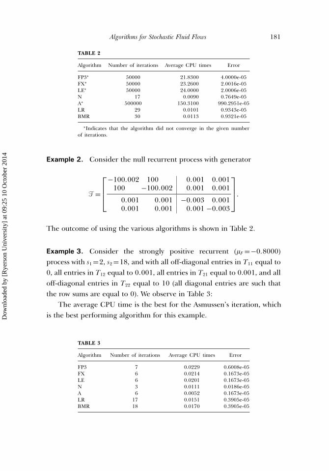
Algorithms for Stochastic Fluid Flows 181
TABLE 2
Algorithm Number of iterations Average CPU times Error
FP3∗ 50000 21.8300 4.0000e-05FX∗ 50000 23.2600 2.0016e-05LE∗ 50000 24.0000 2.0006e-05N 17 0.0090 0.7649e-05A∗ 500000 150.3100 990.2951e-05LR 29 0.0101 0.9343e-05BMR 30 0.0113 0.9321e-05
∗Indicates that the algorithm did not converge in the given numberof iterations.
Example 2. Consider the null recurrent process with generator
� =
−100.002 100 0.001 0.001
100 −100.002 0.001 0.001
0.001 0.001 −0.003 0.0010.001 0.001 0.001 −0.003
.
The outcome of using the various algorithms is shown in Table 2.
Example 3. Consider the strongly positive recurrent (�F =−0.8000)process with s1 =2, s2 =18, and with all off-diagonal entries in T11 equal to0, all entries in T12 equal to 0.001, all entries in T21 equal to 0.001, and alloff-diagonal entries in T22 equal to 10 (all diagonal entries are such thatthe row sums are equal to 0). We observe in Table 3:
The average CPU time is the best for the Asmussen’s iteration, whichis the best performing algorithm for this example.
TABLE 3
Algorithm Number of iterations Average CPU times Error
FP3 7 0.0229 0.6008e-05FX 6 0.0214 0.1673e-05LE 6 0.0201 0.1673e-05N 3 0.0111 0.0186e-05A 6 0.0052 0.1673e-05LR 17 0.0151 0.3905e-05BMR 18 0.0170 0.3905e-05
Dow
nloa
ded
by [
Rye
rson
Uni
vers
ity]
at 0
9:25
10
Oct
ober
201
4
182 Bean, O’Reilly, and Taylor
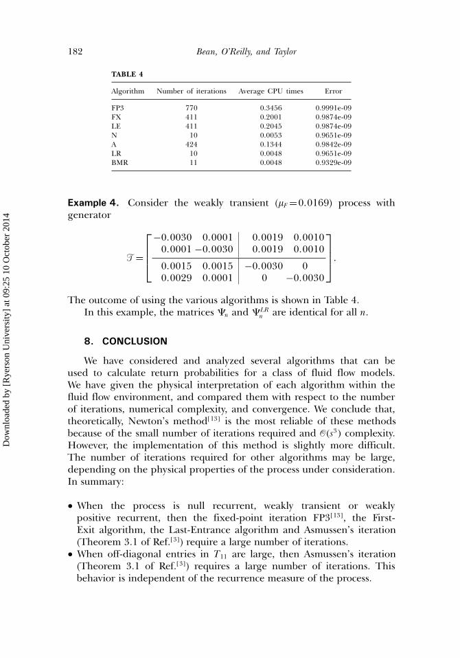
TABLE 4
Algorithm Number of iterations Average CPU times Error
FP3 770 0.3456 0.9991e-09FX 411 0.2001 0.9874e-09LE 411 0.2045 0.9874e-09N 10 0.0053 0.9651e-09A 424 0.1344 0.9842e-09LR 10 0.0048 0.9651e-09BMR 11 0.0048 0.9329e-09
Example 4. Consider the weakly transient (�F =0.0169) process withgenerator
� =
−0.0030 0.0001 0.0019 0.0010
0.0001 −0.0030 0.0019 0.0010
0.0015 0.0015 −0.0030 00.0029 0.0001 0 −0.0030
.
The outcome of using the various algorithms is shown in Table 4.In this example, the matrices �n and � LR
n are identical for all n.
8. CONCLUSION
We have considered and analyzed several algorithms that can beused to calculate return probabilities for a class of fluid flow models.We have given the physical interpretation of each algorithm within thefluid flow environment, and compared them with respect to the numberof iterations, numerical complexity, and convergence. We conclude that,theoretically, Newton’s method[13] is the most reliable of these methodsbecause of the small number of iterations required and �(s3) complexity.However, the implementation of this method is slightly more difficult.The number of iterations required for other algorithms may be large,depending on the physical properties of the process under consideration.In summary:
• When the process is null recurrent, weakly transient or weaklypositive recurrent, then the fixed-point iteration FP3[13], the First-Exit algorithm, the Last-Entrance algorithm and Asmussen’s iteration(Theorem 3.1 of Ref.[3]) require a large number of iterations.
• When off-diagonal entries in T11 are large, then Asmussen’s iteration(Theorem 3.1 of Ref.[3]) requires a large number of iterations. Thisbehavior is independent of the recurrence measure of the process.
Dow
nloa
ded
by [
Rye
rson
Uni
vers
ity]
at 0
9:25
10
Oct
ober
201
4
Algorithms for Stochastic Fluid Flows 183
• When � is large, then both QBD methods require many iterations. Thisis also independent of the recurrence measure of the process.
• In Section 4 we proved that Newton’s method[13] requires less iterationsthan fixed-point iteration FP3[13], the First-Exit algorithm, the Last-Entrance algorithm and Asmussen’s iteration[3].
• We do not have an example in which Newton’s method[13] requiresmore iterations than QBD methods. Our numerical experience suggeststhat when T22 =−�I22, then the Latouche-Ramaswami and Newton’smethods are equivalent, and that Newton’s method requires feweriterations otherwise.
ACKNOWLEDGMENT
The authors would like to thank the Australian Research Council forfunding this research through Discovery Grant number DP0209921. Also,they would like to thank the anonymous referees for making a number ofconstructive suggestions.
REFERENCES
1. Ahn, A.; Ramaswami, V. Transient analysis of fluid flow models via stochastic coupling to aqueue. Stochastic Models. 2004, 20(1), 71–104.
2. Anick, D.; Mitra, D.; Sondhi, M. M. Stochastic theory of a data handling system with multiplesources. Bell System Technical Journal. 1982, 61, 1871–1894.
3. Asmussen, S. Stationary distributions for fluid flow models with or without Brownian noise.Stochastic Models. 1995, 11, 21–49.
4. Bartels, R. H.; Stewart, G. W. Algorithm 432: Solution of the matrix equation AX+XB=C.Communications of the ACM. 1972, 15(9), 820–826.
5. Baase, S. Computer algorithms: introduction to design and analysis; Addison-Wesley PublishingCompany: Reading, Mass., 1978.
6. Bean, N. G.; O’Reilly, M. M.; Taylor, P. G. Hitting probabilities and hitting times for stochasticfluid flows. Submitted.
7. Bhatia, R.; Rosenthal, P. How and why to solve the operator equation AX−XB=Y . Bulletin ofthe London Mathematical Society. 1997, 29, 1–21.
8. Bini, D.; Meini, B. On the solution of a nonlinear matrix equation arising in queueingproblems. SIAM Journal on Matrix Analysis and Applications. 1996, 17(4), 906–926.
9. da Silva Soares, A.; Latouche, G. Further results on the similarity between fluid queues andQBDs. In Eds. G. Latouche and P. Taylor, Matrix-Analytic Methods Theory and Applications; WorldScientific Press: Singapore, 2002; 89–106.
10. Gardiner, J. D.; Laub, A. J.; Amato, J. J.; Moler, C. B. Solution of the Sylvester matrix equationAXBT +CXDT =E. ACM Transactions on Mathematical Software. 1992. 18(2), 223–231.
11. Golub, G. H.; Nash, S.; Van Loan, C. A Hessenberg-Schur method for the problem AX+XB=C. IEEE Transactions on Automatic Control. 1979, 24(6), 909–913.
12. Graham, A. Kronecker Products and Matrix Calculus with Applications; Ellis Horwood Limited:Chichester, 1981.
13. Guo, C-H. Nonsymmetric algebraic Riccati equations and Wiener-Hopf factorization forM-matrices. SIAM Journal on Matrix Analysis and Applications. 2001, 23(1), 225–242.
14. Guo, C-H. A note on the minimal nonnegative solution of a nonsymmetric algebraic Riccatiequation. Linear Algebra and its Applications. 2002, 357, 299–302.
Dow
nloa
ded
by [
Rye
rson
Uni
vers
ity]
at 0
9:25
10
Oct
ober
201
4
184 Bean, O’Reilly, and Taylor
15. Guo, C-H. Convergence analysis of the Latouche-Ramaswami algorithm for null recurrentQuasi-Birth-Death processes. SIAM Journal on Matrix Analysis and Applications. 2002, 23(3),744–760.
16. Guo, C-H.; Laub, A. J. On the iterative solution of a class of nonsymmetric algebraic Riccatiequations. SIAM Journal on Matrix Analysis and Applications. 2000, 22(2), 376–391.
17. Kronsjö, L. I. Algorithms: Their Complexity and Efficiency. John Wiley & Sons: New York, 1979.18. Latouche, G. Newton’s iteration for non-linear equations in Markov chains. IMA Journal of
Numerical Analysis. 1994, 14, 583–598.19. Latouche, G.; Ramaswami, V. Introduction to Matrix Analytic Methods in Stochastic Modeling;
American Statistical Association and SIAM: Philadelphia, PA, 1999.20. Ortega, J. M.; Rheinboldt, W. C. Iterative Solution of Nonlinear Equations in Several Variables;
Academic Press: New York, NY, 1970.21. Ramaswami, V. Matrix analytic methods for stochastic fluid flows. In Proceedings of the 16th
International Teletraffic Congress: Edinburgh, Scotland, June 1999, 1019–1030.22. Rogers, L. C. Fluid models in queueing theory and Wiener-Hopf factorization of Markov
chains. The Annals of Applied Probability. 1994, 4(2), 390–413.23. Seneta, E. Non-negative Matrices and Markov Chains. Springer-Verlag: New York, 1981.24. Varga, R. S. Matrix Iterative Analysis. Prentice-Hall: Englewood Cliffs, NJ, 1962.25. Williams, D. A ‘‘potential theoretic’’ note on the quadratic Wiener-Hopf equation for
Q-matrices. Seminaire de Probabilities XVI, Lecture Notes in Math. 1982, 920, 91–94.
Dow
nloa
ded
by [
Rye
rson
Uni
vers
ity]
at 0
9:25
10
Oct
ober
201
4