algorithmic causal effect identification
TRANSCRIPT
Algorithmic Causal Effect Identification with
causaleffect
Technical Report
Martí PedemonteUniversitat de [email protected]
Jordi VitriàDepartment of Mathematics and Computer Science
Universitat de [email protected]
Álvaro ParafitaDepartment of Mathematics and Computer Science
Universitat de [email protected]
July 13, 2021
Abstract
Our evolution as a species made a huge step forward when we understood the relationshipsbetween causes and effects. These associations may be trivial for some events, but theyare not in complex scenarios. To rigorously prove that some occurrences are caused byothers, causal theory and causal inference were formalized, introducing the do-operatorand its associated rules. The main goal of this report is to review and implement inPython some algorithms to compute conditional and non-conditional causal queries fromobservational data. To this end, we first present some basic background knowledgeon probability and graph theory, before introducing important results on causal theory,used in the construction of the algorithms. We then thoroughly study the identificationalgorithms presented by Shpitser and Pearl in 2006 [SP 2006a, SP 2006b], explaining ourimplementation in Python alongside. The main identification algorithm can be seen asa repeated application of the rules of do-calculus, and it eventually either returns anexpression for the causal query from experimental probabilities or fails to identify thecausal effect, in which case the effect is non-identifiable. We introduce our newly developedPython library and give some usage examples.
Keywords DAG, do-calculus, causality, causal model, identifiability, graph, C-component, hedge,d-separation.
1 Introduction
What is causality? This philosophical concept has dazzled great minds for centuries, and its definition hasbeen debated many times [PM 2018, Chapter 8]. A possible definition is that causality is the influence bywhich one event (a cause) contributes to the production of another event (an effect) where the cause is
This is a revised version of a thesis submitted to the Universitat de Barcelona Department of Mathematics and Computer Science in partialfulfillment of the requirements for the degree of BSc in Computer Science and Software Engineering.
arX
iv:2
107.
0463
2v1
[cs
.MS]
9 J
ul 2
021
Algorithmic Causal Effect Identification Technical Report
partly responsible for the effect, and the effect is partly dependent on the cause. Nevertheless, the conceptand definition of causation is still an ongoing debate between contemporary philosophers, but is out of thescope of this work. Instead, we are interested in how can we answer causal-effect questions, and a veryhelpful concept to have in mind when asking those questions is the Ladder of Causation [PM 2018, Chapter1].
The Ladder of Causation is a metaphor to classify three distinct levels of cognitive ability: seeing, doingand imagining. It consists of three fundamentally different rungs:
Rung 1: Association. This is the first, most basic level of the Ladder of Causation, and it involvesthe observation of data and extraction of regularities from these observations. Examples would behow a dog figures out where a ball is going to land when its owner throws it at the park, or howIBM’s Deep Blue analysed thousands of chess games to extract the moves associated with a higherpercentage of wins. It is characterized by questions like “What if I see...?” or “How would seeing Xchange my belief in Y?”. For instance, what does a survey tell us about the election results? All thequestions related to this level of the Ladder of Causation can be answered using standard statisticalmethods. Note that we cannot answer causal queries, we can only make associations (like, for example,compute the correlation of variables). Many animals and present-day Artificial Intelligence algorithmsare considered to be in this rung.
Rung 2: Intervention. The second level of the Ladder of Causation involves intervening or doing acertain action to produce the desired outcome. Examples would be when we take paracetamol to curea headache (we are intervening on the amount of paracetamol in our body to produce a reduction inheadache pain), or when we study to pass an exam (we act on the things we learn to produce a bettermark in the exam). It is characterized by questions like “What if I do...?” or “How would Y be if I doX?”. For instance, what would be my weight at the end of the year if I were to jog every day for thirtyminutes? To answer questions in this rung of the Ladder of Causation we need to either physicallyperform the intervention or make use of the recently defined do-calculus (which will thoroughly beexplained in this project). Unlike the first level, this one allows us to make causal associations betweenvariables. Babies and also primitive humans that used intentionally-made tools are considered to be inthis rung.
Rung 3: Counterfactuals. The highest level of the Ladder of Causation involves imagination andunderstanding because it compares our real world with an imaginary world. The real world is theworld we live in when we do an action, and the imaginary, counterfactual world is the alternativereality in which my action would have been different. It is characterized by questions like “What if I haddone...?” or “If X had not occurred, would Y have happened?”. For instance, would the Theory of GeneralRelativity had been created if Einstein had not existed? Humankind entered this rung of the Ladderwhen it started to imagine fictional things that they had not seen in real life before, such as divinities,religions or events that could have happened but did not. It is this counterfactual thinking that makesus different from all other intelligent life on Earth and helps us make decisions, by imagining allpossible outcomes.
What is important of this ladder is that one cannot answer queries from a level with information oflower levels alone. For instance, to be able to determine causal effects we do not have enough withonly observational data, we need something else from rung two of the Ladder of Causation (or above).We will use the so-called do-calculus to perform interventions to our probabilities, so instead of havingP(Y|X), which would be read as “the probability of Y when X is seen”, we will have expressions of the formP(Y|do(X)), meaning “the probability of Y when X is artificially imposed”.
This tool will allow us to compute causal effects from observational data, but it will not always work.There will be cases where the mental model of the problem will not allow us to compute these causalrelationships, and we will be forced to either change the model or perform a physical intervention in areal-life experiment. An example where we cannot compute a causal effect between two variables X andY is when there exist some background unmeasurable variables that affect both X and Y. In these caseswhere we cannot use do-calculus to obtain the causal effect, we say that the causal effect is not identifiable orunidentifiable.
2

Algorithmic Causal Effect Identification Technical Report
The goal of this work is to address the identifiability problem (to detect in which cases we can identify acausal effect and in which cases we cannot). To do so we will study a few algorithms devised by Shpitserand Pearl [SP 2006a, SP 2006b] and implement them in Python, developing a package available for everyonein the scientific community to use. In this journey, we will also study thoroughly the necessary resultsused in these algorithms, and we will try to explain them in the most accessible way to reach the widestaudience possible. To this end we have organized this document as follows.
In the first section, we present a succinct historical background of causality, and we explain why this projectis relevant and of general interest.
In section two we present important tools used in the context of causal theory. We first recall some basicprobability theory definitions and theorems, before focusing on crucial aspects about graphs and moreprecisely about direct acyclic graphs (DAGs). We then enter the realm of probabilistic causal models andintroduce do-calculus, an indispensable tool when querying causal effects from experimental observations.We present the identifiability problem, and we end the section by studying some criteria to identify causaleffects through the so-called confounded components.
The third section is devoted to study and explain the implementation of some algorithms that can identifycausal relationships from causal diagrams. We first present the ID algorithm, useful for unconditionalcausal queries, and we explain how we encode probability distributions and causal diagrams in ourimplementation of that algorithm. After having meticulously explored every line of the algorithm alongsideits implementation, we introduce an algorithm to solve conditional causal effects, called IDC. We thenexplain how we have implemented it in our package, and give some examples of how to call these functions.We finalize this third section by concisely giving an idea of how algorithms for counterfactual queries maybe constructed.
Some conclusions on this work are then presented, after which a link with the source code is provided.
2 Why Is the Identification Problem Significant?
For decades causation was seen for most statisticians as a special case of correlation, and we owe thismisleading association to the English statistician 2Sir Francis Galton and especially his disciple, 3KarlPearson. Pearson strongly believed that with data and traditional statistical methods (such as the correlationof variables) one could explain causation. 4Sewall Wright, an American geneticist, was against that beliefand thought that in causal analysis one must incorporate some understanding of the process that producesthe data. He applied this technique when he constructed a path diagram to quantify the influence ofdevelopmental factors in a guinea pig’s womb on the colour of the fur of its offspring. This path diagram,seen now as one of the first causal diagrams (where arrows are drawn from causes to effects), was the kindof resource Pearson was against, for he stated that different (subjective) models would lead to differentconclusions, and that was not rigorous. He could not stand this idea of introducing additional, biasedinformation into the deduction process proposed by Wright, and opposed it outright.
His influence persisted, and it was not until the late 1980’s that causal theory made a significant stepforward. Judea Pearl, an Israeli-American philosopher and computer scientist, was studying how to manageuncertainty in artificial intelligence systems with Bayesian networks, but this approach could not solvecausal-effect queries (recall that one cannot answer questions from rung two of the Ladder of Causationwith just information about rung one). With this problem in mind, he then devoted the following years ofhis career to the formalization of causal theory, obtaining a methodology to compute, in some cases, causaleffects from causal diagrams and observational data.
Before the mathematization of causal theory, some philosophers tried to express the sentence “X causes Y”as “X raises the probability of Y” by writing P(Y|X) > P(Y), but this is wrong at its core. Note that “raises”is a causal concept from the second level of the Ladder of Causation, while the expression P(Y|X) > P(Y)uses data from observations and thus lies on the first level. This inequality really affirms that “if I see X,
2Sir Francis Galton. English statistician, 1822 - 1911.3Karl Pearson. English mathematician and biostatistician, 1857 - 1936.4Sewall Green Wright. American geneticist, 1889 - 1988.
3

Algorithmic Causal Effect Identification Technical Report
then the probability of Y increases”, but this increase in probability could be for other reasons, like a thirdvariable Z being the cause of X and Y.
According to Pearl, who introduced the do-operator, for X to be the cause of Y we need to state that “doingX raises the probability of Y”, which would be written as P(Y|do(X)) > P(Y). This concept of doing orintervening is from rung two, and thus we can borrow this operator to solve causal queries. Note thatdoing is fundamentally different from seeing: by doing X we do not care if a third variable is causing Xand Y because it is I who is forcing the value on X and not some other background factor. If we concludethat the probability of Y while I force the value of X is bigger than without forcing it, then X is partiallyresponsible for Y.
Before the definition of the do-operator we could not solve causal queries because we were simply notasking the correct questions, we did not have the necessary tools to even formulate them. This operator hasnot only allowed us to ask the right questions, but it has also provided us with a set of rules that can helpus resolve these queries. These rules constitute what is known as do-calculus, and under some conditions,they can be used to compute causal effects from observational data. When this is possible, this is, when wecan use do-calculus to compute the effect of a causal relationship, we say that this effect is identifiable.
This definition of identifiability is completely different from the one we have in statistics. In classicalstatistics, a statistical model P = {Pθ |θ ∈ Θ} is identifiable if the mapping θ 7→ Pθ is one-to-one, this is, if fordifferent values of the parameter we obtain different probability distributions. In simultaneous equationsmodels, this problem of identification arises when the value of one or more parameters of the equationsin the model cannot be determined from observable variables. Note that, in this context, identificationdepends profoundly on the equations of the model. The concept of identifiability that Pearl introduceddoes not depend on the form of the equations, but only on the relationship between variables. We willstudy the identification problem in detail in the following section.
But why is the identification problem relevant in the framework of causal models? When trying tocompute a causal effect we could perform the actual intervention in the real world, fixing the value ofa variable X and then measuring the other variable Y, and seeing if P(Y|do(X)) > P(Y). This is notalways feasible, sometimes because it is unethical or sometimes because it is simply not viable. Thereforeit is of great importance to have a way of computing these interventions without having to actuallyperform them in reality. This became possible with the introduction of Pearl’s do-calculus, but lacked asystematic way of calculating causal queries. Years later, a technique to mechanize the estimation of causaleffects was eventually developed. This method takes shape as algorithms, designed by Shpitser and Pearl[SP 2006a, SP 2006b], that use the rules of do-calculus to compute a certain causal effect, when possible,and that raise an error when the causal effect is not identifiable.
Our project will consist of studying thoroughly the theory behind these algorithms to be able to implementthem in Python, and developing a package to perform these causal effect calculations. This work is relevantbecause it gathers a set of recent results which are unknown to many computer scientists and statisticiansin general. Most of them know about do-calculus, but some of them are unaware of the existence ofdeterministic algorithms that mechanize the process of computing causal effects. There are even somescientists who still think that identifiability and the calculation of causal effects is an open problem. Throughthis project we want to reach more people, and to make the extraction of causal effects from observationaldata an effortless procedure.
There is already one implementation of these algorithms for R, by Tikka and Karavanen [TK 2017] underthe name of causaleffect, but we believe that implementing them in Python, a very popular programminglanguage amongst data scientists, will make them more known worldwide. According to the TIOBE index[TIOBE 2021], at the moment of this writing Python is the second most popular programming languagein the whole world just after C, and R falls back to 14th place, so we strongly believe that developing thispackage for Python will boost the popularity of the results by Shpitser and Pearl.
Additionally, with this work we will also try to explain the results that support the algorithms designedby Shpitser and Pearl [SP 2006a, SP 2006b] in a more clear, understandable way. The notation used toformalize causal theory is effective and very well constructed, but lacks transparency, so we believe that,
4

Algorithmic Causal Effect Identification Technical Report
in order to be accessible to a wider audience, results have to be properly organized and formulated in afriendlier way. We tried to do so in this work by first introducing a few necessary concepts of probabilityand graph theory, before entering the world of causal theory.
3 Background Theory
The main purpose of this section is to lay a foundation of definitions and results needed later on in thedefinition and discussion of the algorithms that are the main interest of this work. Some of them canbe found in a standard introductory probability book such as [Ash 1970], others in a basic graph theorybook like [BLW 1986]. The more specific results on causal models and causal diagrams are availablemostly in Causality [Pea 2000] by Judea Pearl and Causal Inference in Statistics [PGJ 2016] by Pearl et al..But there are also some recent results included in this section cited from the original sources, such as[Pea 1993, Pea 1995, SP 2006a, Ver 1993, VP 1988], and for the curious reader, [PM 2018] is a great accessiblebook for wider audiences by the father of modern causality, Judea Pearl.
The first subsection will be focused on establishing and recalling some well-known probability definitionsand basic theorems, for they will be used in the context of probabilistic causal models. Then some basicnotion of graphs will be presented in the second section, given that certain types of graphs are an essentialtool in causality. The section will end with the definition of causal models and causal diagrams, and withthe introduction of a criterion for knowing if a causal effect is identifiable from a causal diagram.
3.1 Probability Theory
To be able to identify causal effects, we must first recall some basic results of probability theory. One couldwonder why probability, a branch of mathematics that works with randomness and doubt, has anythingto do with causality. Perhaps the most common answer would be that we live in a world surroundedby uncertainty, and in every chain of events there are observations we cannot make or factors we cannotcontrol. For instance, the sentence “if you don’t study, you will fail the exam” may be true most of the time,but there are unknown and noisy factors, like chance, luck, or recalling a single memory of that only classyou attended, for example, that may influence the outcome of that exam. That is why the language ofprobabilities is used widely in science to model not only social sciences, but natural sciences as well, andwhy it is also used in causal theory.
Suppose we have an event A. Then the probability P(A) is always bounded between 0 and 1, i.e.,0 ≤ P(A) ≤ 1, where P(A) = 0 when that event is impossible and cannot happen, and P(A) = 1 when Aalways happen. If we now have another event B, the expression P(A, B) refers to the probability of bothevents happening.
A basic result of probability theory is the Law of Total Probability, which will be used to simplify probabilityexpressions in upcoming sections.
Theorem 3.1. (Law of Total Probability) Let A be an arbitrary event, and B1, . . . , Bn mutually exclusive eventssuch that ∑n
i=1 P(Bi) = 1. Then,
P(A) =n
∑i=1
P(A, Bi) .
If B is a binary event, then P(A) = P(A, B) + P(A, B), where B is the complementary of B.
We can also wonder how an event happening influences the probability of another event. To deal withthese dependent probabilities we must state some basic results on conditional probability.
Definition 3.2. (Conditional Probability and Independence) Let A, B two events. Then, the conditionalprobability of A under the condition B, denoted by P(A|B), is the probability that the event A occurs giventhat the event B has already occurred. It can be computed from the probability of joint events,
P(A|B) = P(A, B)P(B)
,
5

Algorithmic Causal Effect Identification Technical Report
which leads to a useful relation to keep in mind, P(A, B) = P(A|B)P(B). We say that two events areindependent if P(A|B) = P(A), meaning that knowing about either event has no effect on the likelihood ofthe other. Using the last derived relation, independence can also be expressed as P(A, B) = P(A)P(B).
Notation. Given two independent events A and B, we will write A ⊥⊥ B. If two events A and B areindependent given a third event C, we will write A ⊥⊥ B|C.
This following result is extremely useful despite its simple formulation, and helps us change fromconditioning on one variable to conditioning on another.
Theorem 3.3. (Bayes’ Theorem) Let A, B two different events with P(B) 6= 0. Then,
P(A|B) = P(B|A)P(A)
P(B).
Proof. From the definition of conditional probability, we have
P(A|B) = P(A, B)P(B)
=P(B, A)
P(B)=
P(B|A)P(A)
P(B).
Notation. We will write P(x|y) as a shorthand for P(X = x|Y = y).
Example 3.4. This example illustrates how we might use the previous stated results and defini-tions to simplify and rewrite probability expressions. Suppose we have the following expression:∑w P(w|z)P(x|z, w)P(y|x, z, w). Then, making use of the derived expression of the conditional proba-bility definition, we can write it as
∑w
P(w|z)P(x|z, w)P(y|x, z, w) = ∑w
P(w|z)P(x, y|z, w) = ∑w
P(x, y, w|z) ,
and by the Law of Total Probability,
∑w
P(x, y, w|z) = P(x, y|z) .
It is sometimes useful to decompose a joint probability into individual, conditional probabilities, becauseif one knows information about the independence between events this procedure may lead to simpler,easier expressions. Nevertheless, the decomposition is obviously not unique. For example, P(x, y, z) =P(x)P(y, z|x) = P(x)P(y|x)P(z|x, y), but also P(x, y, z) = P(z)P(y, x|z) = P(z)P(y|z)P(x|z, y).
This information about dependency between events can be visualized in a graphical form, by drawingprobabilistic graphical models.
Definition 3.5. (Probabilistic Graphical Model) A Probabilistic graphical model is a probabilistic model forwhich a graph shows the conditional dependence between the random variables present in the model. Anexample would be a Bayesian network, which uses directed acyclic graphs to encode variable dependencies.
An example of a probabilistic graphical model is shown below.
Example 3.6. The directed graph in Figure 1 is an example of a probabilistic graphical model, particularlya Bayesian network. This graph encodes the dependencies between three binary variables: whether it issummer, whether it is sunny and whether I wear sunscreen.
Summer
Sunny Sunscreen
Figure 1: Probabilistic graphical model.
6
Algorithmic Causal Effect Identification Technical Report
Clearly, the fact of being summer affects both being a sunny day and my decision to wear sunscreen, butthis is not true in reverse: the season will not change depending on my decision of wearing sunscreen, nortoday being sunny. Additionally, my choice of wearing sunscreen will also depend on the weather, hencethe directed arrow from Sunny to Sunscreen, but I cannot change the weather by putting on some sunscreen(thus the lack of an arrow from Sunscreen to Sunny).
From a Bayesian network one can compute many things, but all from the first rung of the Ladder ofCausation. In such models we only observe the variables of the model, and we do not intervene, which, aswe will see further down this section, is the key to solve causality, a concept from the second rung of theLadder of Causation.
In the previous definition we have talked about directed acyclic graphs, and to understand what they arewe must introduce some concepts on Graph Theory. These will help us not only to deal with Bayesiannetworks but also to establish the foundations of causality.
3.2 Basics of Graph Theory
A very useful tool when talking about causes and effects are graphs, more precisely directed graphs. Notonly they are really intuitive to draw, but they are surprisingly powerful as well, as we will see throughoutthese following sections. The fact that even a six-year-old could sketch a causal diagram (directed graphwhere arrows imply causality from one node to another) and draw some basic conclusions from it makescausality often a mere puzzle. To understand how these causal diagrams are useful we first need to gothrough some results on graph theory.
Definition 3.7. (Graph) A graph is an ordered pair G = (V ,E), where V is a finite not-empty set of verticesor nodes and E ⊂ V × V a set of edges or links that connect some pairs of vertices. Two nodes X and Yconnected by an edge are called adjacent, and we say that X and Y are neighbours. When the edges areordered, represented by X → Y := (X, Y), we have a directed graph. If X and Y are two nodes connected bya directed edge from X to Y (X → Y), we say X is the parent of Y and Y is a child of X.
We can also create new, smaller graphs by selecting only some nodes and edges of a bigger graph.
Definition 3.8. (Subgraph and Induced Subgraph) Let G = (V ,E), G′ = (V ′,E′) be two graphs suchthat V ′ ⊂ V and E′ ⊂ E ∩ (V ′ × V ′). Then, G′ is a subgraph of G, and we denote it by G′ ⊂ G. Ifthe equality E′ = E ∩ (V ′ × V ′) holds, then G′ is the node induced subgraph by the set V ′, and we writeG′ = G[V ′].
It is usually convenient to study not only links between two nodes, but also the paths between twonon-adjacent nodes that are further away.
Definition 3.9. (Path) Let G = (V ,E) be a directed graph and u, v ∈ V two vertices. Consider a sequenceof vertices p = {u = X1, X2, . . . , Xk, Xk+1 = v}, Xi ∈ V ∀i, such that
(a) every pair of consecutive nodes is an edge, i.e., (Xi, Xi+1) ∈ E or (Xi+1, Xi) ∈ E,
(b) all edges joining consecutive nodes in p are different, and
(c) all vertices (except u = X1 and v = Xk+1) are different.
Then, p is a path from u to v (or from v to u). A path that starts and ends at the same node (u = v) is calleda cycle. If any node in the path does not have two incoming or outgoing edges, u has an outgoing edge andv and incoming edge, we say it is a directed path from u to v. If a path is a directed path that starts and endsat the same node (u = v), then it is called a directed cycle. A path from u to v is called a back-door path if itcontains an arrow into u.
A notation that will be exhaustively used all through this project is the concept of parents and children ofnodes in a directed graph.
Definition 3.10. (Parents, Children, Ancestors and Descendants) Let G = (V ,E) be a directed graph andX ⊂ V a subset of nodes. Then, the parents of X , denoted by Pa(X)G, is the set consisting of the parents
7
Algorithmic Causal Effect Identification Technical Report
of every node in X while also containing X . Analogously, the children of X , denoted by Ch(X)G, is theset consisting of the children of every node in X while also containing X . A node Y is an ancestor of anode Xi ∈ X if there exists a directed path p ⊂ G from Y to Xi, and the set of all ancestors of X whilealso containing X is denoted by An(X)G. A node Y is a descendant of a node Xi ∈ X if there exists adirected path p ⊂ G from Xi to Y, and the set of all descendants of X while also containing X is denotedby De(X)G. When possible we will omit the subscript G to ease comprehension.Remark 3.11. Given a directed graph G = (V ,E) and X ⊂ V , it is clear that X ⊂ Pa(X) ⊂ An(X) andX ⊂ Ch(X) ⊂ De(X).
Another useful set of vertices of a graph is the so-called root set, composed by those vertices with nodescendants other than themselves.Definition 3.12. (Root Set) Let G = (V ,E) be a directed graph. Then the root set of G is the set of nodeswith no descendants, Rt(G) = {X ∈ V | De(X)G \ X = ∅}.
As we will see down this section, performing interventions will have the effect of erasing some directededges of a graph. To this end we present the following notation.Notation. Let G = (V ,E) be a directed graph and X ⊂ V . Then we will denote by G
X(resp. GX ) the
graph obtained from G by removing all incoming (resp. outgoing) edges of X .
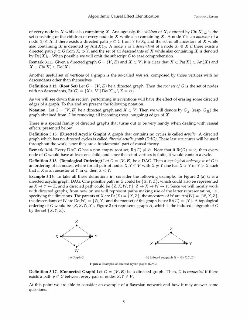
There is a special family of directed graphs that turns out to be very handy when dealing with causaleffects, presented below.Definition 3.13. (Directed Acyclic Graph) A graph that contains no cycles is called acyclic. A directedgraph which has no directed cycles is called directed acyclic graph (DAG). These last structures will be usedthroughout the work, since they are a fundamental part of causal theory.Remark 3.14. Every DAG G has a non empty root set, Rt(G) 6= ∅. Note that if Rt(G) = ∅, then everynode of G would have at least one child, and since the set of vertices is finite, it would contain a cycle.Definition 3.15. (Topological Ordering) Let G = (V ,E) be a DAG. Then a topological ordering π of G isan ordering of its nodes, where for all pair of nodes X, Y ∈ V with X 6= Y one has X > Y or Y > X suchthat if X is an ancestor of Y in G, then X < Y.Example 3.16. To take all these definitions in, consider the following example. In Figure 2 (a) G is adirected acyclic graph, DAG. One possible path in G could be {X, Y, Z}, which could also be representedas X → Y ← Z, and a directed path could be {Z, X, W, Y}, Z → X →W → Y. Since we will mostly workwith directed graphs, from now on we will represent paths making use of the latter representation, i.e.,specifying the directions. The parents of X are Pa(X) = {X, Z}, the ancestors of W are An(W) = {W, X, Z},the descendants of W are De(W) = {W, Y} and the root set of this graph is just Rt(G) = {Y}. A topologicalordering of G would be {Z, X, W, Y}. Figure 2 (b) represents graph H, which is the induced subgraph of Gby the set {X, Y, Z}.
Z
W
X Y
(a) Graph G.
Z
X Y
(b) Induced subgraph H = G[{X, Y, Z}].
Figure 2: Examples of directed acyclic graphs (DAG).
Definition 3.17. (Connected Graph) Let G = (V ,E) be a directed graph. Then, G is connected if thereexists a path p ⊂ G between every pair of nodes X, Y ∈ V .
At this point we are able to consider an example of a Bayesian network and how it may answer somequestions.
8

Algorithmic Causal Effect Identification Technical Report
Example 3.18. Let us retrieve the probabilistic graphical model in Example 3.6. It is the same graph as H inFigure 2 (b), with renamed variables: Z is the binary variable “Summer/Not summer”, X the binary variable“Sunny/Not sunny” and Y the binary variable “I wear sunscreen/I do not wear sunscreen”. It is reasonableto think that the season of the year strongly affects the weather on a particular day (Z → X), and alsothe probability of me wearing sunscreen (Z → Y). Additionally, it is feasible to think that the decision ofwhether or not I must use sunscreen also depends on the weather of that particular day (X → Y). Theconditional probabilities between these random variables can be found in Table 3.
Summer
Yes No0.25 0.75
Sunny
Summer Yes NoYes 0.90 0.10No 0.70 0.30
Sunscreen
Sunny Summer Yes NoYes Yes 0.99 0.01Yes No 0.20 0.80No Yes 0.60 0.40No No 0.05 0.95
Table 3: Conditional probability tables of the different variables of the Bayesian network in example 3.18.
Now, decomposing P(X, Y, Z) into P(X, Y, Z) = P(Y|X, Z)P(X|Z)P(Z), we can use the given conditionalprobabilities to compute, for example, what is the probability of being summer knowing I do wearsunscreen:
P(Z = T|Y = T) =P(Y = T, Z = T)
P(Y = T)=
∑x∈{T,F} P(X = x, Y = T, Z = T)
∑x,z∈{T,F} P(X = x, Y = T, Z = z)=
0.99 · 0.90 · 0.25 + 0.60 · 0.10 · 0.250.99 · 0.90 · 0.25 + 0.60 · 0.10 · 0.25 + 0.20 · 0.70 · 0.75 + 0.05 · 0.30 · 0.75
=0.237750.354
≈ 0.67.
Therefore, the probability that it is summer knowing I wear sunscreen is around 67%, according to theconditional probabilities shown in Table 3 and the dependencies encoded in the Bayesian network in Figure2 (b).
Bayesian networks are a powerful tool to compute probabilities from a dependency graph of variables, butthey do not shed light on the problem of causality. To understand how we can tackle such a puzzle wemust introduce more results, starting with causal models.
3.3 Causal Models
Causal models are a mathematical representation that will help us solve how a first action causes a second,and are the central construction of the algorithms that will be analysed in the following section. But beforeformally defining what a causal model is, consider this plausible made-up example.
Example 3.19. Suppose we want to know how the salary of an employee in a given company depends onthe gender of the worker. It is reasonable to suppose that salary (Y) could depend on the level of education(E) of the employee (better academic records usually translate to higher payroll), the field the employee isworking in (F) and the amount of time he has been working for the company (S for seniority). Clearly, theage (A) of the worker influences both the level of education and the seniority, and gender (X) may have animpact on the seniority as well as the field of the employee. In addition, we might think that both age andgender may be related through a third unobserved variable (U), which could be that perhaps the companyused to hire only men in the past, and thus the average age of men is higher than that of women in thecompany.
The so-called exogenous variables would be the unobserved, unmeasurable variables, U in this example, andthe variables Y, E, F, S, A, X are called endogenous variables. These variables, together with the relations ofdependence described above, form what is known as causal model.
9
Algorithmic Causal Effect Identification Technical Report
Definition 3.20. (Causal Model) A causal model is a triple M = (U ,V ,F ), where:
(a) U is a set of background random variables, called exogenous variables, determined by factors fromoutside the model.
(b) V = {V1, . . . , Vn} is a set of random variables, called endogenous variables, that are determined byvariables in the model, i.e., by variables in U ∪ V .
(c) F = { fi, . . . , fn} is a set of functions such that for every Vi ∈ V , there is a mappingfi : Si ∪ {UVi} → Vi, and such that the whole set F forms a mapping from U to V . That is, for everyVi ∈ V there is a mapping (named structural equation) fi ∈ F such that
Vi = fi(Si, UVi ), i ∈ {1, . . . , n} ,
where UVi ∈ U is the error term linked to Vi, and Si ⊂ (U ∪ V ) \ {Vi, UVi}, known as the parent set.
It is important to emphasise the concept of exogenous variables. Those variables can affect endogenousvariables, which are measurable in our model, but we cannot see nor measure said exogenous variables.They encompass all kinds of unmeasurable perturbations, including the small deviations due to error termsor noise.
Every causal model M has its corresponding directed acyclic graph G = (W ,E), where the node setW = U ∪V contains a node for each observed (endogenous, V ) and unobserved (exogenous, U ) variable ofthe model. We usually ignore the unobservable vertices UVi correspondent to the error term of measurablevariables, for we know that they are always there and are implicitly taken into account in the model.Then, the set of edges E is determined by the functional relationships between the variables in the model,meaning that E contains an edge coming into Vi from every node required to uniquely define fi. Thisgraph G is known as the causal diagram of M.
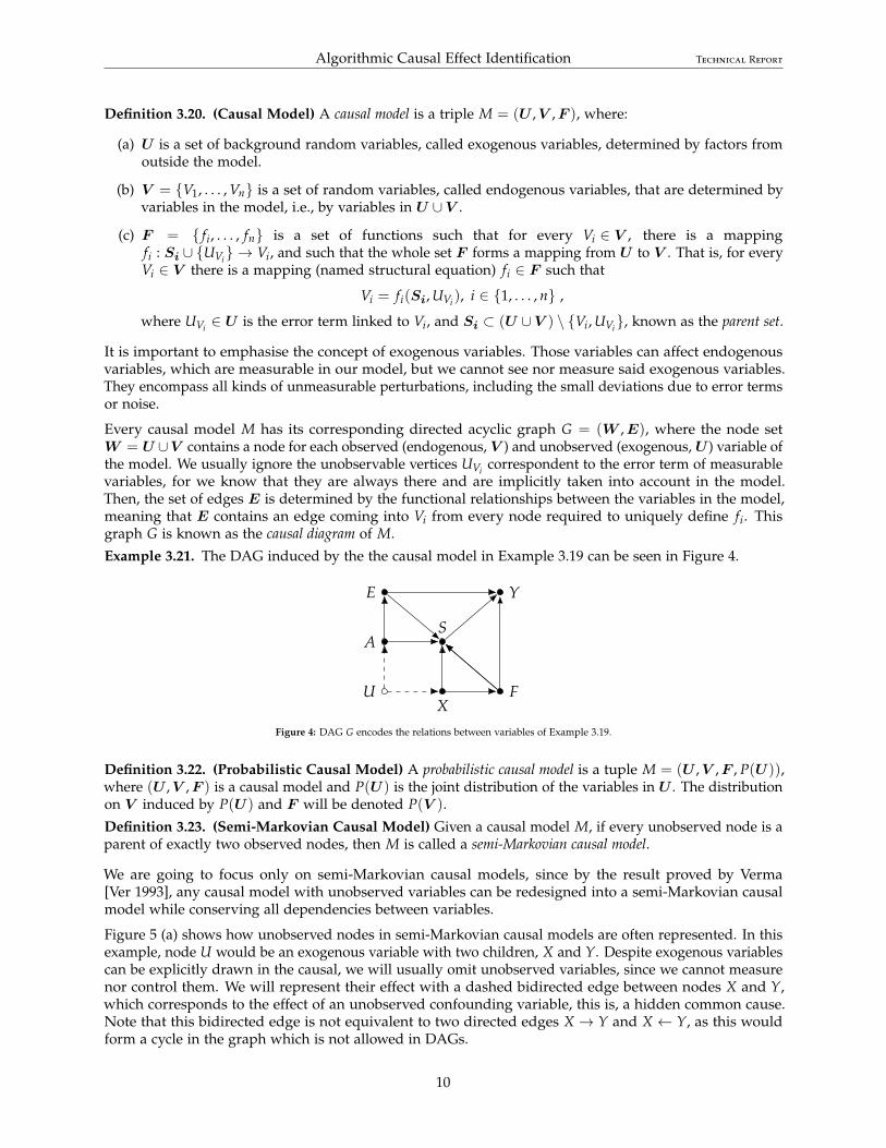
Example 3.21. The DAG induced by the the causal model in Example 3.19 can be seen in Figure 4.
E
A
UX
S
F
Y
Figure 4: DAG G encodes the relations between variables of Example 3.19.
Definition 3.22. (Probabilistic Causal Model) A probabilistic causal model is a tuple M = (U ,V ,F , P(U )),where (U ,V ,F ) is a causal model and P(U ) is the joint distribution of the variables in U . The distributionon V induced by P(U ) and F will be denoted P(V ).
Definition 3.23. (Semi-Markovian Causal Model) Given a causal model M, if every unobserved node is aparent of exactly two observed nodes, then M is called a semi-Markovian causal model.
We are going to focus only on semi-Markovian causal models, since by the result proved by Verma[Ver 1993], any causal model with unobserved variables can be redesigned into a semi-Markovian causalmodel while conserving all dependencies between variables.
Figure 5 (a) shows how unobserved nodes in semi-Markovian causal models are often represented. In thisexample, node U would be an exogenous variable with two children, X and Y. Despite exogenous variablescan be explicitly drawn in the causal, we will usually omit unobserved variables, since we cannot measurenor control them. We will represent their effect with a dashed bidirected edge between nodes X and Y,which corresponds to the effect of an unobserved confounding variable, this is, a hidden common cause.Note that this bidirected edge is not equivalent to two directed edges X → Y and X ← Y, as this wouldform a cycle in the graph which is not allowed in DAGs.
10

Algorithmic Causal Effect Identification Technical Report
U
YX(a)
YX
(b)
Figure 5: (a) U is a confounder of nodes X and Y. (b) We will usually denote confounded nodes with a dashed bidirected edge.
Definition 3.24. (d-separation) Let G = (V ,E) be a DAG, p a path in G and Z a set of nodes Z ⊂ V .Then, the path p is d-separated by the set Z in G if and only if either
(a) p contains a chain I → M→ J or a fork I ← M→ J, such that M ∈ Z and I, J ∈ V , or
(b) p contains an inverted fork or collider I → M← J, such that De(M)G ∩Z = ∅.
Two disjoint sets X and Y are d-separated by Z in G if all paths from X to Y are d-separated by Z in G. Apath that is not d-separated is said to be d-connected.
The following is an important result proved by Verma and Pearl [VP 1988], although we present the clearerand more succinct version proposed by Shpitser and Pearl in [SP 2006a].
Theorem 3.25. (Theorem 1 in [SP 2006a]) Let M be a causal model with the corresponding DAG G = (V ,E),and X ,Y ,Z ⊂ V be sets of variables or nodes in G. If X and Y are d-separated by Z, then X is independent of Ygiven Z in G, i.e., (X ⊥⊥ Y |Z)G.Example 3.26. Consider the DAG G shown in Figure 6, from [Pea 2000, p.p. 17-18]. There are twodifferent paths between X and Y in G, the one that uses the bidirected arc, X → Z1 99KL99 Z3 ← Y, andX → Z1 ← Z2 ← Z3 ← Y. Note that, without measuring {Z1, Z2, Z3}, X and Y are d-separated, since
XZ1 Z2 Z3
Y
Figure 6: DAG G showing d-separation in Example 3.26.
both paths have a collider (X → Z1 ← U, where U is a confounder of Z1 and Z3, and X → Z1 ← Z2).Nevertheless, when Z1 is measured the path X → Z1 99KL99 Z3 ← Y becomes unblocked. This isso because measuring Z = {Z1} unblocks both colliders at Z1 and Z3: at X → Z1 ← U we haveDe(Z1) ∩ {Z1} = {Z1} 6= ∅, and at U → Z3 ← Y we have De(Z3) ∩ {Z1} = {Z1, Z2, Z3} ∩ {Z1} 6= ∅, andthus none of the conditions in Definition 3.24 are met, making X and Y d-connected given Z1.
3.3.1 Causal Effects, do-Calculus and Identifiability
Does smoking cigarettes increase the likelihood of developing lung cancer? This apparently obviousquestion was not that obvious sixty years ago before the foundations of causality were established. Atypical argument against the claim that smoking caused lung cancer was that it could be an unknown“evil” gene confounding the variables “Smoking” and “Lung cancer”, fully accounting for the correlationbetween both variables. Such a gene would make an individual crave nicotine (and thus consume moretobacco) while at the same time would make them prone to developing lung cancer (see Figure 7 (b)).
A randomized controlled trial (RTC) was (and it still is) usually performed in similar problems (for example,in drug testing) to get rid of confounders or other sources of bias. This experiment consists of separatingthe subjects into two or more groups randomly and treating them differently, so one can be sure that thedifferences between them after the experiment are only a product of the different treatments given. The keypoint in these trials is the random selection process, which eliminates (or at least reduces) the biases ofknown and unknown factors. In our situation performing an RTC would not be possible: if both groupswere separated by mere observation and not randomness it would not be an RTC because the “evil” gene
11

Algorithmic Causal Effect Identification Technical Report
“Evil” gene
Smoking Lung cancer
(a)
“Evil” gene
Smoking Lung cancer
(b)
Figure 7: (a) Causal diagram where Smoking is causally related to Lung cancer, while confounded by an “Evil” gene. (b) Causal diagram where Lungcancer is not a causal effect of Smoking.
would be present on most of the smokers, thus inducing a higher probability of cancer in that group. Onthe other hand, creating the groups at random and forcing people to smoke for twenty years to see theirevolution and harming their health in the process is greatly unethical.
We have already stated that to solve problems from the second level of the Ladder of Causation (such ascausal effects queries) we must fix, act on some variables to remove confounder effects. So the point now is,how can we intervene in an experiment without actually physically doing so? The so-called do-operator cansolve this issue.Definition 3.27. (do-operator) Let M = (U ,V ,F , P(U )) be a probabilistic causal model, and X a set ofvariables of the model. Then the do-operator is the intervention that sets the values of X to x, and it is denotedby do(X = x). This is, every action do(X = x) on M produces a new model Mx = (U ,V ,Fx, P(U )),where Fx is obtained by, for every X ∈ X , replacing fX ∈ F with a new constant function of value x givenby do(X = x).Remark 3.28. Despite being apparently similar, we must not misinterpret intervening for conditioning overa variable. P(Y = y|X = x) is the probability that Y = y conditional on finding X = x, in other words,we are considering the distribution of Y among individuals whose X value is x. P(Y = y|do(X = x)),however, is the probability that Y = y when we intervene to make X = x, namely, we are now consideringthe distribution of Y if every individual in the population had their X value fixed at x.Definition 3.29. (Causal Effect) Let M = (U ,V ,F , P(U )) be a probabilistic causal model and X ,Y ⊂ V .Then the causal effect of do(X = x) on Y in M is the marginal distribution of Y in Mx, noted byP(Y |do(X = x)) = Px(Y ).Remark 3.30. For every intervention do(X = x), to ensure that Px(V ) and its marginals are well defined,is required that P(x|Pa(X)G \X) > 0. It is not possible to force X to have values not observed in thedata.
A special case of causal effects are direct effects, where the intervened variables are the parents of thestudied variable.Definition 3.31. (Direct Effect) Given a probabilistic causal model M with variables V and Y ⊂ V , a directeffect is a causal effect of the form P(Y |do(Pa(Y ) \ Y = y′)), this is, when the parents of the variables arethe ones intervened.
The ultimate goal of solving a causal effect problem of some variables X over Y given a causal model Mhas therefore been reduced to finding the probability Px(Y ). Nevertheless, how can we obtain a value forthis probability given that, most of the time, we will only have access to data from observational studies(information of the first rung of the Ladder of Causation)? In 1993 the computer scientist and philosopherJudea Pearl [Pea 1993] showed that, when some conditions are fulfilled, the intervening probability can becomputed from just observational data, making use of the so-called back-door criterion.Definition 3.32. (Back-Door Criterion) Let M = (U ,V ,F , P(U )) be a probabilistic causal model withDAG G and Z ⊂ V , Xi, Xj ∈ V with Xi 6= Xj. Then, we say that Z satisfies the back-door criterion relativeto (Xi, Xj) if:
(a) Z ∩De(Xi) = ∅, and
(b) Z blocks every path between Xi and Xj that contains an arrow into Xi (back-door path).
12

Algorithmic Causal Effect Identification Technical Report
More generally, if X ,Y ⊂ V with X ∩Y = ∅, then Z satisfies the back-door criterion relative to (X ,Y ) if itsatisfies the criterion for every pair (Xi, Xj) ∈ X × Y .
If such a condition is fulfilled, then the next result follows.
Theorem 3.33. (Back-Door Adjustment [Pea 1993]) If a set of variables Z satisfies the back-door criterion relativeto (X ,Y ), then the causal effect of X on Y is given by
Px(y) = ∑z
P(y|x, z)P(z).
Although this criterion was a big step in the right direction, it couldn’t be applied to every scenario, somore adjustments like the previous were required to account for all possible causal diagrams. This dreamof his of obtaining causal information such as Px(Y ) from observational data was finally a reality thanksto the development of do-calculus by Pearl and some of his colleagues in 1995 [Pea 1995]. His theory isconstructed on three simple, yet powerful rules that allow the removal of the do−operator under somespecific scenarios, thus letting one travel from unmeasurable probabilities involving do expressions toobservational, standard probabilities. These rules were first proven by Pearl himself in [Pea 1995].
Theorem 3.34. (Rules of do-Calculus [Pea 2000, Theorem 3.4.1]) Let M = (U ,V ,F , P(U )) be a probabilisticcausal model and G its associated DAG. For any pairwise disjoint subsets of nodes X ,Y ,Z ⊂ V , the following rulesapply:
Rule 1 (Insertion and deletion of observations)
Px(y|z,w) = Px(y|w), if (Y ⊥⊥ Z|X ,W )GX
Rule 2 (Exchanging actions and observations)
Px,z(y|w) = Px(y|z,w), if (Y ⊥⊥ Z|X ,W )GX, Z
Rule 3 (Insertion and deletion of actions)
Px,z(y|w) = Px(y|w), if (Y ⊥⊥ Z|X ,W )GX, Z(W )
where Z(W ) = Z \An (W )GX, i.e., the set of nodes in Z that are not ancestors of any node in W in G
X.
Remark 3.35. Rule 1 of insertion and deletion of observations is a generalization of d-separation (Theorem3.25) in a graph with interventions (that is why independence in G
Xis required). Rule 2 of exchanging
actions and observations is a generalization of the back-door criterion: the only paths in DAG GX ,Z
between Z and Y are back-door paths, and if we block those paths conditioning over X and W we canswap the intervention for the observation. Rule 3 provides conditions for introducing or deleting otherinterventions.
These rules have proven to be enough to compute interventional probabilities whenever these probabilitiescan be identified. Informally speaking, when it is possible to compute the interventional term of adistribution from just observational data, we say that the effect is identifiable.
Theorem 3.36. (do-Calculus Completeness [SP 2006a, Theorem 7]) The three rules of do-calculus, togetherwith standard probability manipulations, are complete for determining identifiability of all effects of the form Px(Y ).
So we know that, if the effect is identifiable, using only the three rules of do-calculus we can obtain analgebraic expression for Px(Y ) which does not involve the do-operator, meaning that we can use onlyobservable data to infer causal conclusions. But what does it really mean for an effect to be identifiable?
Definition 3.37. (Causal Effect Identifiability) Let M = (U ,V ,F , P(U )) be a probabilistic causal modelwith DAG G, and X ,Y ⊂ V . The causal effect of an action do(x) on Y such that X ∩ Y = ∅ is said to beidentifiable from P in G if Px(Y ) is uniquely computable from P(V ) in any causal model which induces G.This is, if for every pair of causal models M1 and M2 such that P1(V ) = P2(V ), the causal effect coincides,P1x(Y ) = P2
x(Y ).
13

Algorithmic Causal Effect Identification Technical Report
In the following example we will use do-calculus to determine the causal effect of a very similar causaldiagram to Figure 7 (a).
Example 3.38. Consider the causal diagram G shown in Figure 8 (a), where the variables S, T and C standfor Smoking, Tar and Cancer. This causal diagram is a slight variation of the one shown in Figure 7 (a).Here, the main modification of the model is that we are supposing that lung cancer only develops throughtar deposited in the lungs (and not from smoking directly), which in turn is only produced by smoking. Inthis scenario, Tar is called a mediator between S and C, because it is the variable that explains the causaleffect of S on C.
ST
C
(a)
ST
C
U
(b)
Figure 8: (a) Causal diagram where Smoking is causally related to Lung cancer through Tar, and Smoking and Cancer confounded. (b) Same causaldiagram but we explicit the unobserved confounder for ease when applying do-calculus.
Our goal is to determine the causal effect Ps(c) from Figure 8. First of all, we use the Law of TotalProbability, followed by some conditional dependence manipulations (similar to Example 3.4):
Ps(c) = P(c|do(s)) = ∑t
P(c, t|do(s)) = ∑t
P(c|t, do(s))P(t|do(s))
Then we apply rule 2 of do calculus, exchanging the t for do(t) in the first term, since (C ⊥⊥ T|S)GS, T(see
Figure 9 (a)):
∑t
P(c|t, do(s))P(t|do(s)) = ∑t
P(c|do(t), do(s))P(t|do(s))
Applying rule 2 again we can change do(s) for s in the second term, because (T ⊥⊥ S)GS (see Figure 9 (b)).The fact that (T ⊥⊥ S)GS follows from Theorem 3.25, since T and S are d-separated in GS by the collider C:
∑t
P(c|do(t), do(s))P(t|do(s)) = ∑t
P(c|do(t), do(s))P(t|s)
We now see that (C ⊥⊥ S|T)GT, S(see Figure 9 (c)), so we can apply rule 3 by deleting the intervention do(s)
from the first term:
∑t
P(c|do(t), do(s))P(t|s) = ∑t
P(c|do(t))P(t|s)
Using some probability axioms as in the first step, we can write:
∑t
P(c|do(t))P(t|s) = ∑s′
∑t
P(c, s′|do(t))P(t|s) = ∑s′
∑t
P(c|do(t), s′)P(s′|do(t))P(t|s)
Using Theorem 3.25 once again we see that (C ⊥⊥ T|S)GT (see Figure 9 (d)), because the chain U → S→ Twhile conditioning on S d-separates the only path between C and T. So using rule 2 once more we canreplace do(t) for t in the first term:
∑s′
∑t
P(c|do(t), s′)P(s′|do(t))P(t|s) = ∑s′
∑t
P(c|t, s′)P(s′|do(t))P(t|s)
14
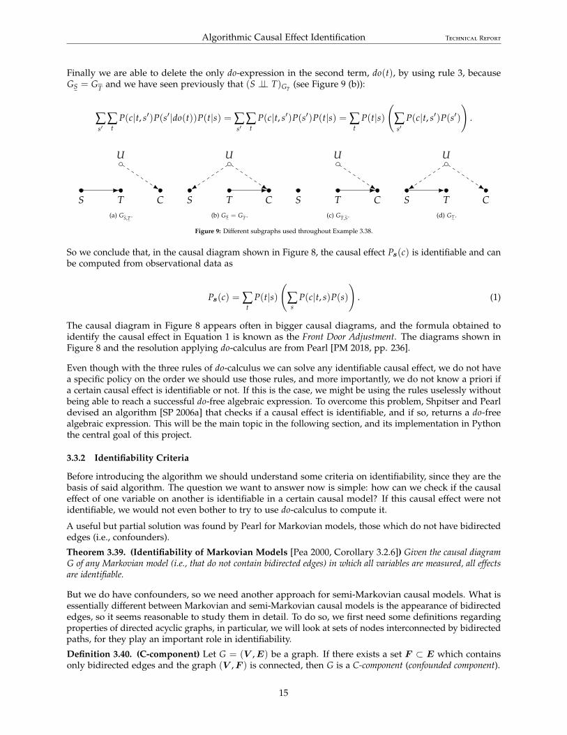
Algorithmic Causal Effect Identification Technical Report
Finally we are able to delete the only do-expression in the second term, do(t), by using rule 3, becauseGS = GT and we have seen previously that (S ⊥⊥ T)GT
(see Figure 9 (b)):
∑s′
∑t
P(c|t, s′)P(s′|do(t))P(t|s) = ∑s′
∑t
P(c|t, s′)P(s′)P(t|s) = ∑t
P(t|s)(
∑s′
P(c|t, s′)P(s′)
).
S T C
U
(a) GS,T .
S T C
U
(b) GS = GT .
S T C
U
(c) GT,S .
S T C
U
(d) GT .
Figure 9: Different subgraphs used throughout Example 3.38.
So we conclude that, in the causal diagram shown in Figure 8, the causal effect Ps(c) is identifiable and canbe computed from observational data as
Ps(c) = ∑t
P(t|s)(
∑s
P(c|t, s)P(s)
). (1)
The causal diagram in Figure 8 appears often in bigger causal diagrams, and the formula obtained toidentify the causal effect in Equation 1 is known as the Front Door Adjustment. The diagrams shown inFigure 8 and the resolution applying do-calculus are from Pearl [PM 2018, pp. 236].
Even though with the three rules of do-calculus we can solve any identifiable causal effect, we do not havea specific policy on the order we should use those rules, and more importantly, we do not know a priori ifa certain causal effect is identifiable or not. If this is the case, we might be using the rules uselessly withoutbeing able to reach a successful do-free algebraic expression. To overcome this problem, Shpitser and Pearldevised an algorithm [SP 2006a] that checks if a causal effect is identifiable, and if so, returns a do-freealgebraic expression. This will be the main topic in the following section, and its implementation in Pythonthe central goal of this project.
3.3.2 Identifiability Criteria
Before introducing the algorithm we should understand some criteria on identifiability, since they are thebasis of said algorithm. The question we want to answer now is simple: how can we check if the causaleffect of one variable on another is identifiable in a certain causal model? If this causal effect were notidentifiable, we would not even bother to try to use do-calculus to compute it.
A useful but partial solution was found by Pearl for Markovian models, those which do not have bidirectededges (i.e., confounders).
Theorem 3.39. (Identifiability of Markovian Models [Pea 2000, Corollary 3.2.6]) Given the causal diagramG of any Markovian model (i.e., that do not contain bidirected edges) in which all variables are measured, all effectsare identifiable.
But we do have confounders, so we need another approach for semi-Markovian causal models. What isessentially different between Markovian and semi-Markovian causal models is the appearance of bidirectededges, so it seems reasonable to study them in detail. To do so, we first need some definitions regardingproperties of directed acyclic graphs, in particular, we will look at sets of nodes interconnected by bidirectedpaths, for they play an important role in identifiability.
Definition 3.40. (C-component) Let G = (V ,E) be a graph. If there exists a set F ⊂ E which containsonly bidirected edges and the graph (V ,F ) is connected, then G is a C-component (confounded component).
15

Algorithmic Causal Effect Identification Technical Report
Definition 3.41. (Maximal C-component) Let G be a graph and S = (V ,E) a C-component with S ⊂ G.Then S is a maximal C-component (with respect to G) if, for every bidirected path in G containing at leastone node of V , that path is also a path in S.
If G is not a C-component, it can be uniquely partitioned into a set of graphs, each a maximal C-componentwith respect to G.Lemma 3.42. Every directed graph G = (V ,E) can be decomposed into a unique set C(G) = {G[S1], . . . , G[Sk]}of subgraphs such that every G[Si] ∀i ∈ {1, . . . , k} is a maximal C-component of G.
Proof. Given two nodes X, Y ∈ V , they belong to the same maximal C-component if and only if there existsa bidirected path between X and Y, from the definition of maximal C-component. Therefore every maximalC-component is unique, hence the bidirected paths of G define its maximal C-components.
This decomposition will ultimately help us to reduce the identification problem into several smalleridentification subproblems. A useful special case of C-components are C-trees, which are closely related todirect effects.Definition 3.43. (C-tree) Let G = (V ,E) be a C-component such that every node has at most one child. Ifthere exists a node X ∈ V such that An(X)G = V , then G is a X-rooted C-tree.
The following is just a generalization of a C-tree with multiple roots.Definition 3.44. (C-forest) Let G = (V ,E) be a C-component such that every node has at most one child.Then, if X = Rt(G), i.e., if X have no descendants, we say G is a X-rooted C-forest.
If a DAG contains a pair of different C-forests, under some conditions this pair of C-forests are called ahedge, structures that play a fundamental part in identifiability.Definition 3.45. (Hedge) Let G = (V ,E) be a directed graph, and X ,Y ⊂ V disjoint sets of nodes,i.e., X ∩ Y = ∅. Suppose that there exist two R-rooted C-forests F = (VF,EF), F̃ = (VF̃,EF̃) such thatX ∩ VF 6= ∅, X ∩ VF̃ = ∅, F̃ ⊆ F and R ⊂ An(Y )G
X. Then, F and F̃ form a hedge for Px(y) in G.
Example 3.46. Figure 10 (a) shows a causal diagram G of a probabilistic causal model M. It can easily beseen that G is not a C-component, because its bidirected edges do not connect all vertices in G. Nevertheless,G can be decomposed into three maximal C-components, G[S1] and G[S2], as seen in Figures 10 (b) and(c), and also the trivial component G[S3] = {X5}, which is the graph containing X5 with no edges. Thesethree C-components are, in turn, also C-trees, because every node in G[S1], G[S2] and G[S3] has at mostone child: G[S1] is a X4-rooted C-tree, since An(X4)G[S1]
= {X1, X2, X3, X4}, G[S2] is a X6-rooted C-tree,for An(X6)G[S2]
= {X6, X7}, and finally G[S3] is a X5-rooted C-tree.
We can also detect a hedge for Px1(x6) in G. We can easily see that G[S1] is a {X4}-rooted C-forest with{X1} ∩ S1 6= ∅ and {X4} ⊂ An(X6)GX1
. Now consider F, the {X4}-rooted C-forest formed only by thevertex X4 and no edges. It is clear that {X1} ∩ VF = {X1} ∩ {X4} = ∅, and that F ⊆ S1. Therefore, G[S1]and F form a hedge for Px1(x6) in G.
X1
X2
X3
X4
X5
X6
X7
(a) Graph G.
X1
X2
X3
X4
(b) Maximal C-component G[S1] ⊂ G.
X6
X7
(c) Maximal C-component G[S2] ⊂ G.
Figure 10: Causal diagram G contains three maximal C-components, G[S1], G[S2] and G[S3], that are also C-trees.
The following result is finally what we were searching for in this section, a criterion to check if a causaleffect is identifiable.
16
Algorithmic Causal Effect Identification Technical Report
Theorem 3.47. (Hedge Identifiability Criterion [SP 2006a, Theorem 4]) Let G be the causal diagram of a modelM = (U ,V ,F , P(U )), and X ,Y ⊂ V . Then the causal effect Px(y) is not identifiable in G if and only if thereexist two R-rooted C-forests F and F̃ that form a hedge for Px(y) in G.
Knowing this we can state that the causal effect Px1(x6) is not identifiable in Figure 10 (a), since we haveseen in Example 3.46 that there is a hedge for Px1(x6).
Remark 3.48. In Example 3.46 we have introduced a well-known non-identifiable graph, G[S2], whichis the so-called bow arc graph. It is the simplest non-identifiable graph, easily provable with the hedgecriterion. Consider the {X6}-rooted C-forests G[S2] and {X6}, which clearly form a hedge for Px7(x6) inG[S2].
A complete characterization of identifiability involves hedges, and will be the discussed in the comingsection.
4 Identification Algorithms and Their Implementation
do-calculus was the first step into solving causal effects from causal diagrams, but it has a major problem:even if the effect is identifiable, no one tells us in what order should we apply the three rules, and this getseven more complex when the number of variables in the model grows.
In this section, we will introduce two algorithms that help us compute causal queries, when those areidentifiable, called ID and IDC. We will examine meticulously each and every line of both algorithms,justifying why the operations involved are correct, while also explaining our implementation in Python.This implementation is the central objective of this project, and all objects and functions involved form anewly developed package for Python named causaleffect.
We will first introduce an algorithm to solve non-conditional causal effects and its implementation, then wewill do the same for an algorithm to compute conditional causal effects. To conclude this section we willshortly explain the existence of some algorithms to compute counterfactual queries from interventionaldistributions, which have not been developed in our package.
4.1 Identification of Interventional Distributions
We have seen that if the causal diagram G of a causal model M is not a C-component it can be decomposedinto a unique set of maximal C-components (Lemma 3.42). This in turn will help to reduce the identificationproblem in more manageable subproblems, making use of the following result by Jin Tian [Tian 2002].
Lemma 4.1. ([Tian 2002, Corollary 1 pp. 56]) Let G = (V ,E) be the induced DAG from the causal modelM = (U ,V ,F , P(U )), and C(G) = {G[S1], . . . , G[Sk]} a decomposition of G in C-components, where Si are thevertices in G[Si]. Then, we have
(a) P(v) factorizes as
P(v) =k
∏i=1
P(si|do(v \ si)) =k
∏i=1
Pv\si(si) .
(b) Let a topological order over V be V1 < · · · < Vn, and let V (i)G = {V1, . . . , Vi} for 1 ≤ i ≤ n, and V
(0)G = ∅.
Then every factor from the previous product is identifiable in G as
Pv\sj (sj) = ∏{i|Vi∈Sj}
P(vi|v(i−1)G )
We are now able to define the identification algorithm presented in Figure 11.
17
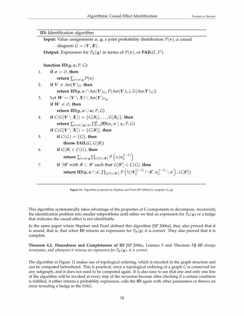
Algorithmic Causal Effect Identification Technical Report
ID: Identification algorithmInput: Value assignments x, y, a joint probability distribution P(v), a causal
diagram G = (V ,E).Output: Expression for Px(y) in terms of P(v), or FAIL(F, F′).
function ID(y,x, P, G):1. if x = ∅, then
return ∑v∈v\y P(v)2. if V 6= An(Y )G, then
return ID(y,x∩An(Y )G, P(An(Y )G), G[An(Y )G])3. Let W = (V \X) \An(Y )GX
if W 6= ∅, thenreturn ID(y,x∪w, P, G)
4. if C(G[V \X ]) = {G[S1], . . . , G[Sk]}, thenreturn ∑v∈v\(y∪x) ∏k
i=1ID(si,v \ si, P, G)if C(G[V \X ]) = {G[S]}, then
5. if C(G) = {G}, thenthrow FAIL(G, G[S])
6. if G[S] ∈ C(G), then
return ∑v∈s\y ∏{i|Vi∈S} P(
vi|v(i−1)G
)
7. if ∃S ′ with S ⊂ S ′ such that G[S ′] ∈ C(G), then
return ID(y,x∩ s′, ∏{i|Vi∈S′} P(
Vi|V (i−1)G ∩S ′,v(i−1)
G \ s′)
, G[S ′])
Figure 11: Algorithm proposed by Shpitser and Pearl [SP 2006a] to compute Px(y).
This algorithm systematically takes advantage of the properties of C-components to decompose, recursively,the identification problem into smaller subproblems until either we find an expression for Px(y) or a hedgethat indicates the causal effect is not identifiable.
In the same paper where Shpitser and Pearl defined this algorithm [SP 2006a], they also proved that itis sound, that is, that when ID returns an expression for Px(y) it is correct. They also proved that it iscomplete.
Theorem 4.2. (Soundness and Completeness of ID [SP 2006a, Lemma 3 and Theorem 5]) ID alwaysterminates, and whenever it returns an expression for Px(y), it is correct.
The algorithm in Figure 11 makes use of topological ordering, which is encoded in the graph structure andcan be computed beforehand. This is practical, since a topological ordering of a graph G is conserved forany subgraph, and it does not need to be computed again. It is also easy to see that one and only one lineof the algorithm will be invoked at every step of the recursion because after checking if a certain conditionis fulfilled, it either returns a probability expression, calls the ID again with other parameters or throws anerror revealing a hedge in the DAG.
18
Algorithmic Causal Effect Identification Technical Report
Before seeing in more detail every line of the algorithm and how it has been implemented we will showhow the algorithm operates given a causal diagram. To do so, consider again the causal diagram introducedin Example 3.38.
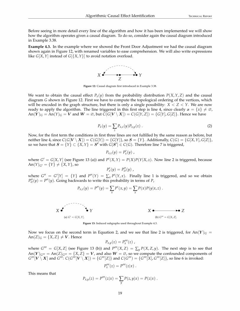
Example 4.3. In the example where we showed the Front Door Adjustment we had the causal diagramshown again in Figure 12, with renamed variables to ease comprehension. We will also write expressionslike G[X, Y] instead of G[{X, Y}] to avoid notation overload.
XZ
Y
Figure 12: Causal diagram first introduced in Example 3.38.
We want to obtain the causal effect Px(y) from the probability distribution P(X, Y, Z) and the causaldiagram G shown in Figure 12. First we have to compute the topological ordering of the vertices, whichwill be encoded in the graph structure, but there is only a single possibility: X < Z < Y. We are nowready to apply the algorithm. The line triggered in this first step is line 4, since clearly x = {x} 6= ∅,An(Y )G = An(Y)G = V and W = ∅, but C(G[V \X ]) = C(G[Y, Z]) = {G[Y], G[Z]}. Hence we have
Px(y) = ∑z
Px,z(y)Px,y(z) . (2)
Now, for the first term the conditions in first three lines are not fulfilled by the same reason as before, butneither line 4, since C(G[V \X ]) = C(G[Y]) = {G[Y]}, so S = {Y}. Additionally, C(G) = {G[X, Y], G[Z]},so we have that S = {Y} ⊂ {X, Y} = S′ with G[S′] ∈ C(G). Therefore line 7 is triggered,
Px,z(y) = P′x(y) ,
where G′ = G[X, Y] (see Figure 13 (a)) and P′(X, Y) = P(X)P(Y|X, z). Now line 2 is triggered, becauseAn(Y)G′ = {Y} 6= {X, Y}, so
P′x(y) = P′′∅(y) ,
where G′′ = G′[Y] = {Y} and P′′(Y) = ∑x P′(Y, x). Finally line 1 is triggered, and so we obtainP′′∅(y) = P′′(y). Going backwards to write this probability in terms of P,
Px,z(y) = P′′(y) = ∑x
P′(x, y) = ∑x
P(x)P(y|x, z) .
X Y(a) G′ = G[X, Y].
X Z(b) G′′′ = G[X, Z].
Figure 13: Induced subgraphs used throughout Example 4.3.
Now we focus on the second term in Equation 2, and we see that line 2 is triggered, for An(Y )G =An(Z)G = {X, Z} 6= V . Hence
Px,y(z) = P′′′x (z) ,
where G′′′ = G[X, Z] (see Figure 13 (b)) and P′′′(X, Z) = ∑y P(X, Z, y). The next step is to see thatAn(Y )G′′′ = An(Z)G′′′ = {X, Z} = V , and also W = ∅, so we compute the confounded components ofG′′′[V \X ] and G′′′: C(G′′′[V \X ]) = {G′′′[Z]} and C(G′′′) = {G′′′[X], G′′′[Z]}, so line 6 is invoked:
P′′′x (z) = P′′′(z|x) .
This means thatPx,y(z) = P′′′(z|x) = ∑
yP(z, y|x) = P(z|x) .
19

Algorithmic Causal Effect Identification Technical Report
Putting together the two terms of Equation 2 we finally obtain the desired causal effect:
Px(y) = ∑z
(∑x
P(x)P(y|x, z)
)P(z|x) = ∑
zP(z|x)∑
xP(x)P(y|x, z) .
Indeed, we obtain the same result as in Example 3.38, as we see that Equation 1 is identical to the oneobtained using the identification algorithm with renamed variables {X = S, Z = T, Y = C}.
ID algorithm in Figure 11 can also be used to detect unidentifiability. We are going to see another exampleof the algorithm that raises an error due to the existence of a hedge.
Example 4.4. Consider the DAG G in Figure 14 (a), and we will to compute Px(y). The only possibletopological order would be X < Z < W < Y, and we see that the ancestors of Y in G are all the nodes in G.
X
Z
Y
W
(a) Graph G.
X
Z
W
(b) G′ = G[X, W, Z].
Figure 14: Causal diagrams in Example 4.4.
First of all, line 4 will be executed, because the ancestors of Y (in G and in GX) is the set containing allvertices of G and also C(G[V \ X]) = {G[Y], G[W], G[Z]}. So we will have
Px(y) = ∑w,z
Px,w,z(y)Px,y,z(w)Px,y,w(z) . (3)
For the first term, line 6 is triggered, because G[Y] ∈ C(G) = {G[Y], G[X, W, Z]}, so
Px,w,z(y) = P(y|x, w, z) .
The second term invokes line 2, because Y /∈ An(W)G, thus we obtain
Px,y,z(w) = Px,z(w) ,
where G′ = G[X, W, Z] (see Figure 14 (b)) and P′(X, W, Z) = ∑y P(X, W, Z, y). Now we have C(G′[W]) =
{G′[W]} and C(G′) = {G′}, so line 5 is triggered, throwing the hedge (G′, G′[W]) for Px,z(w) in G′. Clearlyboth are C-components of G′, they are W-rooted (with W being an ancestor of Y in G′
X), G′[W] ⊂ G′,
G′ ∩ {X} 6= ∅ and G′[W] ∩ {X} = ∅. So we conclude that (G′, G′[W]) form a hedge for Px,z(w) in G′, andthus the original causal effect Px(y) is not identifiable in G.
We are now ready to explore in detail every line of the algorithm and to show our implementation of ID inPython.
4.1.1 Python Implementation of Graphs and Distributions
First of all, to handle graphs and probabilities we need some classes. In our implementation to deal withgraphs we have used the igraph library for Python since it provides some useful methods (although, as wewill see, we will also need to implement our own).
The first thing we need to be able to do is to create a DAG in a simple, intuitive way. For this purpose, wedevised the function createGraph (see Function 1).
Another useful function that helps visualize causal diagrams that we have implemented is plotGraph (seeFunction 2).
20

Algorithmic Causal Effect Identification Technical Report
def createGraph(edges, verbose=False):Description Creates a Graph object from a list of edges in string format.Parameters edges List of edges of the graph. Each edge must either be directed (’X->Y’)
or bidirected (’X<->Y’).verbose Boolean. If enabled, some useful debugging information will be printed.
Returns A Graph object from the igraph library, with the directed and bidirected edgesgiven as the edges parameter. Each bidirected edge will be encoded as two directededges. It will contain exactly all vertices appearing in the edges list. Each edgewill have a property called confounding, which will be 0 for directed edges and±1 for bidirected edges (edges of a bidirected pair will have opposite signs for theconfounding property).
Function 1: Implemented createGraph function.
def plotGraph(graph, name=None):Description Plots a causal diagram. Needs pycairo library.Parameters graph Graph object with an edge property named confounding.
name Name of the png file with the plotted graph. If not introduced it doesnot produce a png image.
Returns Nothing. It makes use of the function plot of the igraph library to plot the causaldiagram.
Function 2: Implemented plotGraph function.
To ease the comparison of causal effects of different causal models between our implementation the onemade with R by Tikka and Karvanen [TK 2017], we have created a function that “translates” our edgenotation into theirs (see Function 3).
def to_R_notation(edges):Description Converts a list of edges from our notation to the notation used in the R package
causaleffect.Parameters edges List of strings containing the edges of a graph.Returns Tuple of three elements. The first is a string encoding the edges of a graph. The next
two elements are integers, and are the indexes used by the causaleffect package toset confounding properties to the edges of the graph.
Function 3: Implemented to_R_notation function.
To see how these three functions work we can create the causal diagram in Figure 14 (a) by executing thecode in Figure 15 (a).
The output of the plot of graph G can be seen in Figure 15 (b), where bidirected edges are coloured ingreen and are slightly thinner than directed edges.
We have developed many more functions to obtain properties of causal diagrams needed in the implemen-tation of ID, but they will be explained in due course when required by the algorithm. The next step is tomanage distribution probabilities. For that purpose, we have created a Python class named Probability,which can be constructed recursively to embrace the nature of the algorithm, also recursive.
The Probability class has several attributes. The string sets var and cond allow simpleconditional distributions (distributions of var conditioned on cond). For instance, the objectProbability(var={'Y'}, cond={'X'}) represents the distribution P(Y|X). To model products of distribu-tions, and mimicking [TK 2017], the boolean attribute recursive is defined, allowing multiple Probabilityobjects to be nested inside one another when True. When this is the case, the attribute children, which is aset, is filled with Probability objects, and the variables var and cond are ignored. We can now have more
21

Algorithmic Causal Effect Identification Technical Report
>>> edges = ['X<->Z', 'X<->W', 'X->Z', 'Z->W', 'W->Y', 'X->Y']
>>> G = createGraph(edges)
>>> print(to_R_notation(edges))
('X-+Z, Z-+W, W-+Y, X-+Y, X-+Z, X+-Z, X-+W, X+-W', 5, 8)
>>> plotGraph(G)
(a) Code executed.
(b) Plot of graph G.
Figure 15: Executing createGraph, to_R_notation and plotGraph.
complex probability distributions such as P∗(X, Y, Z, W) = P(Z, X|W)P(Y|Z)P(W) by creating the objectin Figure 16 (a).
p1 = Probability(var={'X', 'Z'}, cond={'W'})
p2 = Probability(var={'Y'}, cond={'Z'})
p3 = Probability(var={'W'})
p = Probability(recursive=True , children ={p1, p2, p3})
(a) P∗(X, Y, Z, W).
p1 = Probability(var={'X', 'Z'}, cond={'W'})
p2 = Probability(var={'Y'}, cond={'Z'})
p3 = Probability(var={'W'})
p4 = Probability(sumset ={'X', 'Z', 'W'}, recursive=True , children ={p1, p2, p3})
p = Probability(sumset ={'Z', 'W'}, recursive=True , children ={p1, p2, p3}, fraction=
True , divisor=p4)
(b) P∗(X|Y).
Figure 16: Representing probability distributions with the Probability class.
We also need to consider how to manage marginal distributions, and thus a set containing variables to besummed over (in the discrete case, integrated in the continuous case) is defined. The attribute sumset is theset of variables that makes this possible. So if we wanted to represent P∗(X, Y), we would need to set theattribute sumset={'Z', 'W'} for the object p previously defined.
Another level of complexity is needed when computing conditional probabilities. Sometimes to formconditional distribution expressions one has to introduce fractions, and that is why the Probability classhas two last attributes, fraction and divisor. When the boolean attribute fraction is set to True, thedivisor containing a probability distribution object is enabled. This final step allows us to represent
22
Algorithmic Causal Effect Identification Technical Report
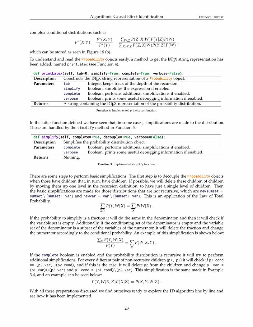
complex conditional distributions such as
P∗(X|Y) = P∗(X, Y)P∗(Y)
=∑W,Z P(Z, X|W)P(Y|Z)P(W)
∑X,W,Z P(Z, X|W)P(Y|Z)P(W),
which can be stored as seen in Figure 16 (b).
To understand and read the Probability objects easily, a method to get the LATEX string representation hasbeen added, named printLatex (see Function 4).
def printLatex(self, tab=0, simplify=True, complete=True, verbose=False):Description Constructs the LATEX string representation of a Probability object.Parameters tab Integer, keeps track of the depth of the recursion.
simplify Boolean, simplifies the expression if enabled.complete Boolean, performs additional simplifications if enabled.verbose Boolean, prints some useful debugging information if enabled.
Returns A string containing the LATEX representation of the probability distribution.
Function 4: Implemented printLatex function.
In the latter function defined we have seen that, in some cases, simplifications are made to the distribution.Those are handled by the simplify method in Function 5.
def simplify(self, complete=True, decouple=True, verbose=False):Description Simplifies the probability distribution object.Parameters complete Boolean, performs additional simplifications if enabled.
verbose Boolean, prints some useful debugging information if enabled.Returns Nothing.
Function 5: Implemented simplify function.
There are some steps to perform basic simplifications. The first step is to decouple the Probability objectswhen those have children that, in turn, have children. If possible, we will delete these children of childrenby moving them up one level in the recursion definition, to have just a single level of children. Thenthe basic simplifications are made for those distributions that are not recursive, which are newsumset =sumset \ (sumset ∩ var) and newvar = var \ (sumset ∩ var). This is an application of the Law of TotalProbability,
∑X,Y
P(Y, W|X) = ∑X
P(W|X) .
If the probability to simplify is a fraction it will do the same in the denominator, and then it will check ifthe variable set is empty. Additionally, if the conditioning set of the denominator is empty and the variableset of the denominator is a subset of the variables of the numerator, it will delete the fraction and changethe numerator accordingly to the conditional probability. An example of this simplification is shown below:
∑X P(Y, W|X)
P(Y)= ∑
XP(W|X, Y) .
If the complete boolean is enabled and the probability distribution is recursive it will try to performadditional simplifications. For every different pair of non-recursive children (p1, p2) it will check if p1.cond== (p2.var)∪(p2.cond), and if this is the case, it will delete p2 from the children and change p1.var =(p1.var)∪(p2.var) and p1.cond = (p1.cond)\(p2.var). This simplification is the same made in Example3.4, and an example can be seen below:
P(Y, W|X, Z)P(X|Z) = P(X, Y, W|Z) .
With all these preparations discussed we find ourselves ready to explore the ID algorithm line by line andsee how it has been implemented.
23

Algorithmic Causal Effect Identification Technical Report
4.1.2 Python Implementation of the ID Algorithm
We have already reviewed how graphs and probability distribution objects will be encoded in our im-plementation, and later on, when used, some useful functions regarding these objects will be explained.The function implementing the ID algorithm in Figure 11 in our package is called ID_rec, referring to itsrecursive nature (see Function 6).
def ID_rec(Y, X, P, G, ordering, verbose=False, tab=0):Description Recursive function that implements the identification algorithm ID, computing the
causal effect Px(y) of a DAG G.Parameters Y Set of strings containing the variables in y.
X Set of strings containing the intervened variables in x.P Probability object with the probability distribution P.G Graph object, encoding the DAG of the causal model G.ordering List of strings containing a topological ordering of the nodes of G.verbose Boolean, prints some useful debugging information if enabled.tab Integer, keeps track of the depth of the recursion.
Returns If the effect is identifiable it returns a Probability object with de computed causaleffect Px(y). If the algorithm encounters a hedge it raises an error, providing the twoforests that form the hedge for Px(y) in G.
Function 6: Implemented ID_rec function.
When the function is called it first retrieves all vertices of G and stores them as a set in a variable V. It thenseparates the graph G in the directed (only containing directed edges) and the bidirected (only containingbidirected edged) parts, calling the developed function get_directed_bidirected_graphs in Function 7.
def get_directed_bidirected_graphs(G):Description Decouples the causal diagram G into two separate graphs: one containing only
bidirected edges, and the other containing directed edges.Parameters G Graph object G.Returns A tuple with two Graph objects (one with bidirected edges and the other with directed
edges).
Function 7: Implemented get_directed_bidirected_graphs function.
The observed portion of G will be saved as G_dir. We now proceed to explain every line of the algorithmin detail, revealing our implementation.
Line 1
1. if x = ∅, thenreturn ∑v∈v\y P(v)
This line is rather straightforward, since we do not have the do-operator any more (x = ∅). Therefore,we are computing the marginal distribution P(y) instead of a causal effect. This action of marginalizingconsiders two cases: if the probability distribution is simple, this is, if it is not a product of probabilities,changes the variables of P to the variables in y. If, on the contrary, the probability is a product ofprobabilities, adds the pertinent variables to the sum set, sumset = sumset∪ (V \ Y).Line 2
2. if V 6= An(Y )G, thenreturn ID(y,x∩An(Y )G, P(An(Y )G), G[An(Y )G])
24

Algorithmic Causal Effect Identification Technical Report
This line eliminates all non-ancestors of Y in G. To see clearly how this is possible, consider the followingresult.
Lemma 4.5. ([SP 2006a, Lemma 5]) Let X ′ = X ∩An(Y )G. Then, Px(y) obtained from P in G is equal toP′x′(y) obtained from P′ = P(An(Y )G) in G[An(Y )G].
Proof. Let W = V \An(Y )G, and consider the submodel Mw, i.e., where the variables in W are intervened.The induced causal diagram is G[V \W ] = G[An(Y )G], and the induced distribution is P′ = Pw(An(Y )G).
Now let X ′′ = X \An(Y )G, and clearly X = X ′ tX ′′. Therefore, we have
Px(y) = Px′ ,x′′(y) = Px′(y) ,
where in the last equality we have used rule 3 of do-calculus. Indeed, note that we have(Y ⊥⊥ X ′′|X ′)G
X ′ , X ′′= (Y ⊥⊥ X ′′|X ′)GX
, because there are no paths from Y to X ′′: directed pathsfrom X ′′ to Y are non-existing because, by definition, X ′′ has no ancestors of Y , and back-door paths aredeleted by removing all incoming edges to X ′′ ⊂ X in G
X. We apply rule 3 of do-calculus again, finally
obtainingPx′(y) = Px′ ,w(y) = P′x′(y) ,
because (Y ⊥⊥W |X ′)GX ′ , W
. By the same reasoning as before, there are no directed paths from W =
V \An(Y )G to Y , neither back-door paths (deleted by looking at GX ′ ,W ).
To implement this line, we first have developed a function to compute the ancestors of a node or a set ofnodes (see Function 8).
def get_ancestors(G, V):Description Computes the set containing all ancestors of a vertex or a set of vertices, including
itself.Parameters G Graph object, encoding the direct portion of the causal diagram G (which
is a DAG).V String with the name of a vertex, or a set of strings containing the names
of the vertices.Returns A set of strings containing the names of vertices in G which are ancestors of V.
Function 8: Implemented get_ancestors function.
If a single vertex is inputted, Function 8 computes its ancestors by exploring the directed acyclic graphusing BFS (breadth-first search). If, on the other hand, a set of vertices is given, it calls itself for every singlevertex in the set and performs the union of the results.
To check if the condition in line 2 is fulfilled we compute the ancestors of Y in G and save it as anc, beforequerying the length of the set V \ anc. If this length is not zero, we create a Probability object which isthe marginalized distribution of the one given (considering the two cases discussed in line 1), and we callID_rec again with the new parameters specified. The only parameter worth mentioning is the inducedsubgraph, G[An(Y )G], which we have computed using the function induced_subgraph from the igraphlibrary for efficiency purposes. This function takes a graph and a set of nodes and constructs a subgraphwith all given nodes and edges between them as in the original graph.
Line 3
3. Let W = (V \X) \An(Y )GX
if W 6= ∅, thenreturn ID(y,x∪w, P, G)
This line adds interventions to the original causal effect, which is possible due to rule 3 of do-calculus.
25
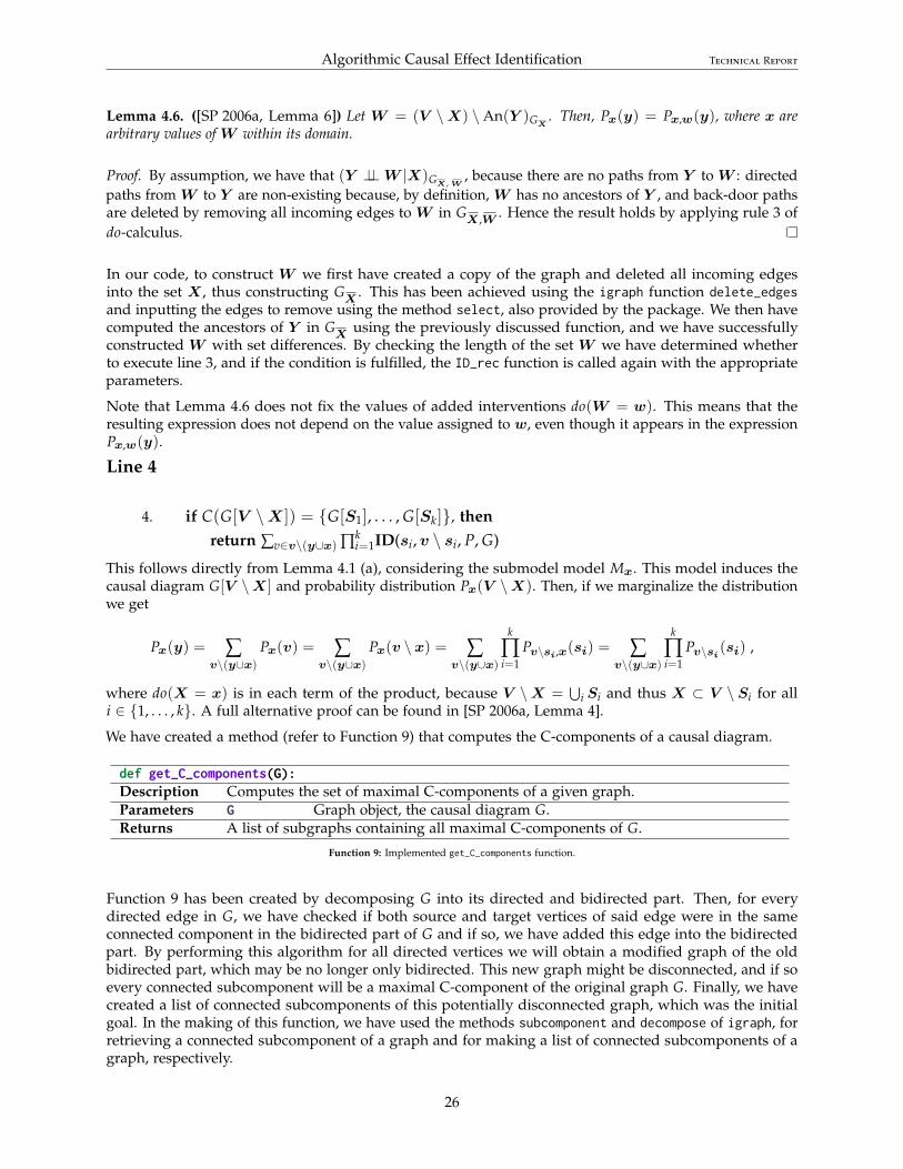
Algorithmic Causal Effect Identification Technical Report
Lemma 4.6. ([SP 2006a, Lemma 6]) Let W = (V \X) \An(Y )GX. Then, Px(y) = Px,w(y), where x are
arbitrary values of W within its domain.
Proof. By assumption, we have that (Y ⊥⊥W |X)GX, W, because there are no paths from Y to W : directed
paths from W to Y are non-existing because, by definition, W has no ancestors of Y , and back-door pathsare deleted by removing all incoming edges to W in G
X ,W . Hence the result holds by applying rule 3 ofdo-calculus.
In our code, to construct W we first have created a copy of the graph and deleted all incoming edgesinto the set X , thus constructing G
X. This has been achieved using the igraph function delete_edges
and inputting the edges to remove using the method select, also provided by the package. We then havecomputed the ancestors of Y in G
Xusing the previously discussed function, and we have successfully
constructed W with set differences. By checking the length of the set W we have determined whetherto execute line 3, and if the condition is fulfilled, the ID_rec function is called again with the appropriateparameters.
Note that Lemma 4.6 does not fix the values of added interventions do(W = w). This means that theresulting expression does not depend on the value assigned to w, even though it appears in the expressionPx,w(y).
Line 4
4. if C(G[V \X ]) = {G[S1], . . . , G[Sk]}, thenreturn ∑v∈v\(y∪x) ∏k
i=1ID(si,v \ si, P, G)
This follows directly from Lemma 4.1 (a), considering the submodel model Mx. This model induces thecausal diagram G[V \X ] and probability distribution Px(V \X). Then, if we marginalize the distributionwe get
Px(y) = ∑v\(y∪x)
Px(v) = ∑v\(y∪x)
Px(v \ x) = ∑v\(y∪x)
k
∏i=1
Pv\si,x(si) = ∑v\(y∪x)
k
∏i=1
Pv\si(si) ,
where do(X = x) is in each term of the product, because V \X =⋃
i Si and thus X ⊂ V \ Si for alli ∈ {1, . . . , k}. A full alternative proof can be found in [SP 2006a, Lemma 4].
We have created a method (refer to Function 9) that computes the C-components of a causal diagram.
def get_C_components(G):Description Computes the set of maximal C-components of a given graph.Parameters G Graph object, the causal diagram G.Returns A list of subgraphs containing all maximal C-components of G.
Function 9: Implemented get_C_components function.
Function 9 has been created by decomposing G into its directed and bidirected part. Then, for everydirected edge in G, we have checked if both source and target vertices of said edge were in the sameconnected component in the bidirected part of G and if so, we have added this edge into the bidirectedpart. By performing this algorithm for all directed vertices we will obtain a modified graph of the oldbidirected part, which may be no longer only bidirected. This new graph might be disconnected, and if soevery connected subcomponent will be a maximal C-component of the original graph G. Finally, we havecreated a list of connected subcomponents of this potentially disconnected graph, which was the initialgoal. In the making of this function, we have used the methods subcomponent and decompose of igraph, forretrieving a connected subcomponent of a graph and for making a list of connected subcomponents of agraph, respectively.
26

Algorithmic Causal Effect Identification Technical Report
The length of the set containing the maximal C-components of G[V \X ] will determine if line 4 is triggeredor not. If invoked, a set of probabilities will be filled by calling the ID_rec function again, with the properparameters, one time for each C-component. If identifiable, each ID_rec call will return a Probabilityobject, stored in the set of probabilities aforementioned. Finally, a recursive Probability object will bereturned, with the set of probabilities as children and the pertinent sumset.
If line 4 has not been triggered, then there is only one C-component, C(G[V \X ]) = {G[S]}, so lines 5, 6or 7 will be executed.
Line 5
5. if C(G) = {G}, thenthrow FAIL(G, G[S])
The discovery of a hedge in G for Px(y) is the only source of unidentifiability in the algorithm. Theconditions of line 5 imply the existence of a hedge for the current recursion stage, as it states the followingTheorem.
Theorem 4.7. ([SP 2006a, Theorem 6]) Suppose that line 5 in ID is executed. Then there exist X ′ ⊆ X andY ′ ⊆ Y such that the graph pair G, G[S] returned by the fail condition of ID contain as edge subgraphs twoC-forests F, F′ that form a hedge for Px′(y′).
Proof. Let R the root set of G (which in this step of the recursion will be a subgraph of the original input).Since G is a single C-component, it is possible to remove a set of directed arrows from G while preservingthe root set R such that the resulting graph F is an R-rooted C-forest (i.e., such that each node has at mostone child). Additionally, by lines 2 and 3 of the algorithm, we know that R ⊂ An(Y )GX
.
Now consider the graph F′ = F ∩ G[S], which is also an R-rooted C-forest because only single directedarrows were removed from G[S] to obtain F′. Moreover we know that F′ ⊂ F, VF ∩X 6= ∅ and VF′ ∩X = ∅by construction, so we have a hedge for X and Y , a subset of the original input.
In our source code we have called once again the function get_C_components for the original graph. If itonly produces a single maximal C-component it must be the graph itself, so by checking the length ofthe set of maximal C-components of G we decide whether to invoke line 5. If so, it raises a HedgeFoundexception, which returns information about the pair (G, G[S]).
Line 6
6. if G[S] ∈ C(G), then
return ∑v∈s\y ∏{i|Vi∈S} P(
vi|v(i−1)G
)
This line also follows from Lemma 4.1, but this time from part (b). If line preconditions are met, thisis, if C(G[V \X ]) = {G[S]}, then V \X = S follows. This implies that G local to that recursive call ispartitioned into G[S] ∈ C(G) and G[X ], with no bidirected arcs between these two partitions, and thatX = V \S. Therefore,
Px(y) = Pv\s(y) = ∑s\y
Pv\s(s) = ∑s\y
∏{i|Vi∈S}
P(vi|v(i−1)G ) ,
where the last equality follows from Lemma 4.1 (b) given that G[S] ∈ C(G).
Note that in line 4 we could not use Lemma 4.1 (b) for each product term Pv\si(si) as we have done herebecause, unlike this case, we did not know if G[Si] ∈ C(G).
To implement this line of the algorithm we must first check if G[S] ∈ C(G), and we have constructed afunction called check_subcomponent that does just that: it iterates through a list of graphs, called components,and returns True if a given graph is in that list. The complicated part is to create a function to compare
27

Algorithmic Causal Effect Identification Technical Report
graphs, this is, to analyse if two graphs are equal. This function, named graphs_are_equal in our package,has been implemented relying on another function, check_subgraph (see Function 10), that checks if a givengraph G1 is a subgraph of another graph G2, G1 ⊆ G2. Provided with this function, to see if two graphs
def check_subgraph(G1, G2):Description Given two graphs G1 and G2 this function verifies if G1 ⊆ G2.Parameters G1 Graph object, with both directed and bidirected parts.
G2 Graph object, with both directed and bidirected parts.Returns A boolean whose value is True if G1⊆G1, False otherwise.
Function 10: Implemented check_subgraph function.
are equal we just have to see if G1 ⊆ G2 and G2 ⊆ G1, and that is precisely what the graphs_are_equalfunction does.
Function 10 first checks if the set of nodes of G1 is a subset of the set of nodes of G2, and then looks if thenumber of edges of G1 is larger than the number of edges in G2. If the former condition is not satisfied orthe latter is fulfilled, the function would immediately return False. Then it checks if every edge in G1 isalso in G2, and if all edges of G1 satisfy the prior condition, returns True. If even a single edge in G1 is notin G2, it would return False.
If the condition of line 6 is fulfilled, we have to consider two different cases. The first one is when S consistsof a single vertex (|S| = 1) and hence we do not have a product of probabilities (the Probability object toreturn will not be recursive but instead very simple). We will obtain the conditional vertices in v
(i−1)G by
calling the get_previous_order method defined in Function 11.
def get_previous_order(v, possible, ordering):Description This function computes the vertices prior to a given one in a certain topological
ordering. It excludes the given vertex and all other vertices not present in the possibleset of vertices passed.
Parameters v String, name of the initial vertex of the topological ordering.possible Set of possible vertices that can be in the output set.ordering List of vertices containing an ordering of the graph G.
Returns A set of vertices strictly smaller than the given vertex in the given topological ordering,intersected with the possible vertices set.
Function 11: Implemented get_previous_order function.
Once we have the conditional variables of the output Probability object we must construct said object. Ifthe probability distribution in the recursive call is simple and only consists of a single term, the outputprobability distribution will be also very simple. For example, if P′(X, Y, Z) = P(X, Y, Z) and we wantto calculate P′(Y|X, Z), it is just P(Y|X, Z). But if the given distribution is a little bit more complex andconsists of a product or sums of probabilities the output distribution will also be complex. For instance,consider the previous example but with P′(X, Y, Z) = P(X, Y)P(Z). Now we would have
P′(Y|X, Z) =P′(X, Y, Z)
P′(X, Z)=
P′(X, Y, Z)∑Y P′(X, Y, Z)
=P(X, Y)P(Z)
∑Y P(X, Y)P(Z)=
P(X, Y)P(Z)P(X)P(Z)
= P(Y|X) .
To take this into account we have devised a function named get_new_probability (explained in Function12).
The simplest case is when cond = ∅. In this scenario, if the given distribution is not recursive we onlychange the variables of the old distribution for var, while if it is a product of probabilities we add thevariables V \ var in the sum set (marginalizing). By contrast, if cond 6= ∅, we construct a new Probability
object which is a fraction of the form∑V\(var∪cond) P′
∑V\cond P′ , equal to P′(var|cond) = P′(var∪cond)P′(cond) . Before returning
this probability we attempt to perform a simplification using simplify (Function 5).
28

Algorithmic Causal Effect Identification Technical Report
def get_new_probability(P, var, cond={}):Description Function that computes a conditional probability from a distribution P = P′ of the
form P′(var|cond).Parameters P Probability object, with a probability distribution P′.
var Set of variables of the new distribution.cond Set of conditional variables of the new distribution.
Returns A Probability object from the given distribution P′ encoding P′(var|cond).Function 12: Implemented get_new_probability function.
Once we have this new probability, this first case of line 6 can return that Probability object summed overS \ Y .
We have considered when S has only one element, and the remaining case when S has two or moreelements is now simple. We construct a set of probabilities, and for each vertex in S we create a Probabilityobject in the same manner as in the first scenario. Then we construct and return a recursive Probabilityobject with this set of probabilities as children, and summed over S \ Y .
Line 7
7. if ∃S ′ with S ⊂ S ′ such that G[S ′] ∈ C(G), then
return ID(y,x∩ s′, ∏{i|Vi∈S′} P(
Vi|V (i−1)G ∩S ′,v(i−1)
G \ s′)
, G[S ′])
This line covers the last possible outcome. If the algorithm has reached this far it is clear that C(G) hasmore than one C-component (otherwise line 5 would have been triggered), and that G[S] is not a maximalC-component of G (or then line 6 would have been executed). Therefore there are bidirectional edgesbetween G[S] and G[X ] in G, and so there has to be a maximal C-component of G, G[S′], such thatG[S] ⊂ G[S′]. The equivalence of intervened probabilities in line 7 relays on the following result.
Lemma 4.8. ([SP 2006a, Lemma 8]) If the conditions of line 7 of ID are satisfied, Px obtained from P in G is equalto P′x∩s′ obtained from P′ = ∏{i|Vi∈S′} P
(Vi|V (i−1)
G ∩S′,v(i−1)G \ s′
)in G[S′].
The implementation we have devised is somewhat similar to the one performed in line 6. First it checks, foreach component G[S′j ] in C(G), if G[S] ⊂ G[S′j ], by iterating over the components in C(G) and using thecheck_subgraph function earlier defined (see Function 10). Once it has found the maximal C-component ofG that satisfies G[S] ⊂ G[S′] ∈ C(G), it splits again the possible cases in |S′| = 1 and |S′| > 1.
When |S′| = 1, we get the smaller vertices V(i−1)
G using the get_previous_order function (Function 11),and perform the intersections, differences and unions necessary according to the conditional variables ofthe new probability stated by line 7. Next, using these conditional variables, we compute a new probabilitydistribution as we did in line 6, by using function get_new_probability (Function 12). We finally return arecursive call to ID_rec with Y , X ∩S′, the new probability distribution and the induced subgraph G[S′](using induced_subgraph from the igraph library).
When |S′| > 1 we define a set of probabilities and for each vertex in S′ we create a Probability object inthe same fashion as in the case |S′| = 1. We finally construct a recursive Probability object with this set ofprobabilities as children, which will be the distribution passed in the recursive call to ID_rec. All the otherparameters of this recursive call are the same as in the first scenario.
We have checked all lines of the ID algorithm, and since it is sound and complete, there are no more casesto explore. Our implementation of this algorithm, named ID_rec in the developed package, consequentlyfinishes here. Despite being very useful in the majority of cases, this algorithm only computes identifiablecausal effects of the form Px(y), but we could also think of conditional interventions. Shpitser and Pearl,authors of the recently explained identification algorithm, devised also an algorithm for such cases, as weexplain in the following section.
29

Algorithmic Causal Effect Identification Technical Report
4.2 Identification of Conditional Interventional Distributions
We have seen an algorithm to compute the causal effect of the form Px(y), but often we know that somevariables hold, that is, the distribution is conditioned on a set of other variables. We now consider theproblem of identifying distributions of the form Px(y|z), where X ,Y and Z are disjoint sets of variables.The basic idea is to reduce the problem to a solved case when Z = ∅, so we can use the algorithm IDseen in the former section. A possible way to do so is to use rule 2 of do-calculus, that exchanges actionsand observations, Px,z(y|w) = Px(y|z,w), under some conditions, and that is how the algorithm IDC isconstructed. This conditional identification algorithm is presented in Figure 17.
IDC: Conditional identification algorithmInput: Value assignments x, y and z, a joint probability distribution P(v), a
causal diagram G = (V ,E).Output: Expression for Px(y|z) in terms of P(v), or FAIL(F, F′).
function IDC(y,x, z, P, G):1. if ∃Z′ ∈ Z such that (Y ⊥⊥ Z′|X ,Z \ {Z′})GX, Z′ , then
return IDC(y,x∪ {z′}, z \ {z′}, P, G)2. else let P′ = ID(y ∪ z,x, P, G),
return P′∑y P′
Figure 17: Algorithm proposed by Shpitser and Pearl [SP 2006b] to compute Px(y|z).
Similarly to the first identification algorithm, Shpitser and Pearl defined this algorithm in [SP 2006b] andthey also proved that it is sound and complete.
Theorem 4.9. (Soundness and Completeness of IDC [SP 2006b, Theorem 7 and Theorem 8]) IDC alwaysterminates, and whenever it returns an expression for Px(y|z), it is correct.
The first line of the IDC is a direct application of rule 2 of do-calculus where the exchange consistsof a single variable {Z′}, because if (Y ⊥⊥ Z′|X ,Z \ {Z′})GX, Z′ , then Px(y|z) = Px(y|z \ {z′}, {z′}) =
Px∪{z′}(y|z \ {z′}) follows.
The full construction and justification of the conditional identification algorithm can be found in [SP 2006b].
4.2.1 Python Implementation of the IDC Algorithm
Having seen how we represent graphs and probability distribution objects, and how the ID algorithmworks (which is an essential requirement), we are ready to reveal our implementation of IDC in Figure 17.In our package, algorithm IDC is called IDC, and it is defined in Function 13.
We are now going to explain in detail how we have implemented these two lines of algorithm IDC in ourpackage.
Line 1In the first line we have to see if there is a vertex Z′ in Z fulfilling the independence suggested. To do so,we must first obtain the graph in which this independence will be checked, and note that the graph isdifferent for each vertex Z′ in Z. Therefore, we first loop through the vertices in Z, and then for each onewe construct the required graph. To do so, we first use a newly defined function called unobserved_graph,explained in Function 14.
Function 14 changes the representation of a graph we have used up to this point to a more explicitrepresentation, where exogenous variables confounding two nodes are now nodes in the graph object.
30

Algorithmic Causal Effect Identification Technical Report
def IDC(Y, X, Z, P, G, ordering, verbose=False, tab=0):Description Recursive function that implements the conditional identification algorithm IDC,
computing the causal effect Px(y|z) of a DAG G, by using the rule 2 of do-calculusand the ID algorithm.
Parameters Y Set of strings containing the variables in y.X Set of strings containing the intervened variables in x.Z Set of strings containing the conditional variables in z.P Probability object with the probability distribution P.G Graph object, encoding the DAG of the causal model G.ordering List of strings containing a topological ordering of the nodes of G.verbose Boolean, prints some useful debugging information if enabled.tab Integer, keeps track of the depth of the recursion.
Returns If the conditional causal effect is identifiable it returns a Probability object with decomputed causal effect Px(y|z). If the algorithm encounters a hedge it raises an error,providing the two C-forests that form the hedge for Px(y|z) in G.
Function 13: Implemented IDC function.
def unobserved_graph(G):Description Function that constructs a causal diagram where confounded variables have explicit
unmeasurable nodes from a DAG of bidirected edges.Parameters G Graph object, encoding the DAG of the causal model G with bidirected
edges.Returns A graph object with no bidirected confounding edges, but instead explicit exogenous
variables and direct edges to the the affected nodes.
Function 14: Implemented unobserved_graph function.
This is necessary for the next steps (deleting arrows and computing d-separation of two sets of nodes), aswe will see next, but let us first show how a graph object representation is changed when applying thisfunction, by considering Figure 18.
(a) Graph with bidirected edges confounding variables. (b) Graph with explicit unmeasurable confounders.
Figure 18: We always use the graph representation in (a), but for the purposes of checking d-separation we must explicitly state the direct arrows fromconfounders to variables as in (b).
In Figure 18 (a) we see the plot of a graph object where the pairs of variables (X, W) and (X, Z) areconfounded by hidden common causes. We see that, after applying the unobserved_graph function, theseunobserved common causes appear explicitly, named WX for the first pair and ZX for the second, in Figure18 (b). Note that this explicit representation will only be used to compute d-separation of sets of measurablevariables, and nowhere else.
31

Algorithmic Causal Effect Identification Technical Report
The following step is to remove incoming edges to X and outgoing edges from Z′. This is wherethe previously constructed graph comes into play: imagine we have to remove outgoing edges from aconfounded vertex X. In the first representation we would delete a directed confounding edge from thebidirected pair (see Figure Figure 19 (a)), while in reality a variable that is confounded only has incomingedges, not outgoing! To see this more clearly, consider Figure 19, where all outgoing edges of X have beendeleted.
YX
(a) Bidirected representation.
XY
YX(b) Explicit representation.
Figure 19: X and Y are confounded by an exogenous variable XY, and outgoing edges from X have been deleted (incorrectly in (a)).
In Figure 19, if we were to remove outgoing edges from X in the bidirected representation we would bedeleting an arrow that it really does not exist. In reality, X has no outgoing edges, and we need the explicitrepresentation to be aware of this.
In our implementation, we have deleted the appropriate incoming and outgoing edges from the explicitversion of G as stated in line 1, using the delete_edges and select functions provided by igraph, as wedid in line 3 of ID. Then we have checked if Y and Z′ are independent conditional to X and Z \ {Z′} inthe modified graph, (Y ⊥⊥ Z′|X ,Z \ {Z′})GX, Z′ , by using Theorem 3.25 and seeing if they are d-separated.To do so, we have constructed Function 15, named dSep.
def dSep(G, Y, node, cond, verbose=False):Description Checks if the set Y and the node node are d-separated in G conditional to a set of
nodes cond.Parameters G Graph object, encoding the DAG of the causal model G.
Y Set of strings containing some nodes in G.node String, node of the graph G.cond Set of strings containing some nodes in G.verbose Boolean, prints some useful debugging information if enabled.
Returns Returns True if all paths between Y and the node node conditional to cond in G ared-separated, False if there is a d-connected path between a node in Y and node.
Function 15: Implemented dSep function.
Function 15 iterates through all possible paths between all nodes of Y and node, and for each path itcomputes if it is d-separated. To do so we have devised a function to verify if a given path in a graph isd-separated by a set of vertices, called is_path_d_separated (see Function 16).
def is_path_d_separated(G, path, cond, verbose=False):Description Checks if a given path path is d-separated in G conditional to a set of nodes cond.Parameters G Graph object, encoding the DAG of the causal model G.
path List if indexes of vertices in G, consisting of a path between the first andlast elements of the list.
cond Set of strings containing some nodes in G.verbose Boolean, prints some useful debugging information if enabled.
Returns Returns True if the path conditional to cond in G is d-separated, False if it is d-connected.
Function 16: Implemented is_path_d_separated function.
32

Algorithmic Causal Effect Identification Technical Report
To certify that a path is d-separated in Function 16 we have iterated through the vertices of the path, lookingfor the necessary structures that make a path d-separated (see Definition 3.24). This is, we have looked foreither a chain or a fork with a node of the conditional set in the middle (I → M→ J or I ← M→ J withM ∈ cond and I, J ∈ path), or for a collider with no descendants in the conditional set (i.e., I → M ← Jwith De(M)G ∩ cond = ∅). Therefore, as we did with the ancestors, we have also created Function 17 tocompute the descendants of a set of nodes, called get_descendants.
def get_descendants(G, V):Description Computes the set containing all descendants of a vertex or a set of vertices, including
itself.Parameters G Graph object, encoding the direct portion of the causal diagram G (which
is a DAG).V String with the name of a vertex, or a set of strings containing the names
of the vertices.Returns A set of strings containing the names of vertices in G which are descendants of V.
Function 17: Implemented get_descendants function.
Analogously to the get_ancestors function, if a single vertex is inputted, Function 17 computes itsdescendants by exploring the directed acyclic graph using BFS (breadth-first search). If, on the other hand,a set of vertices is given, it calls itself for every single vertex in the set and performs the union of the results.
Once we know, using the aforementioned functions, that there is a vertex Z′ such that(Y ⊥⊥ Z′|X ,Z \ {Z′})GX, Z′ , we simply call recursively the function IDC with exactly the same param-eters except for the fact that now Z′ is in the do set instead of the conditional set (following line 1 of thealgorithm IDC).
Line 2This second line of IDC is really straightforward, as we do not have to check any condition. We just callthe function of the first identification algorithm, ID_rec, with the specified parameters, and then createa fractional Probability object with the numerator being the returned probability from ID_rec and thedenominator the same but summed over the variables in y.
4.3 Join Implementation of ID and IDC and Usage
In our package we have decided to join the two identification algorithms in just one function, named ID(refer to Function 18).
def ID(Y, X, G, cond={}, verbose=False):Description Function that calls either the non-conditional (ID) or the conditional (IDC) identifica-
tion algorithm, depending on the parameter cond.Parameters Y Set of strings containing the variables in y.
X Set of strings containing the intervened variables in x.G Graph object, encoding the DAG of the causal model G.cond Set of strings containing the conditional variables.verbose Boolean, prints some useful debugging information if enabled.
Returns If the parameter cond is empty, this is, if it does not contain any element, the ID_recfunction is called. Otherwise, if it contains any element, then IDC is executed.
Function 18: Implemented ID function.
Function 18 is the one in charge of checking if the the three sets of vertices inputted are pairwise disjoint,as required by both algorithms, and if the directed part of the graph is a DAG. Then it creates the firstProbability object by setting all the nodes in G as the variables of the distribution. It is also the one thathas to compute a topological ordering of the vertices in G, which as we recall only has to be computed once.
33
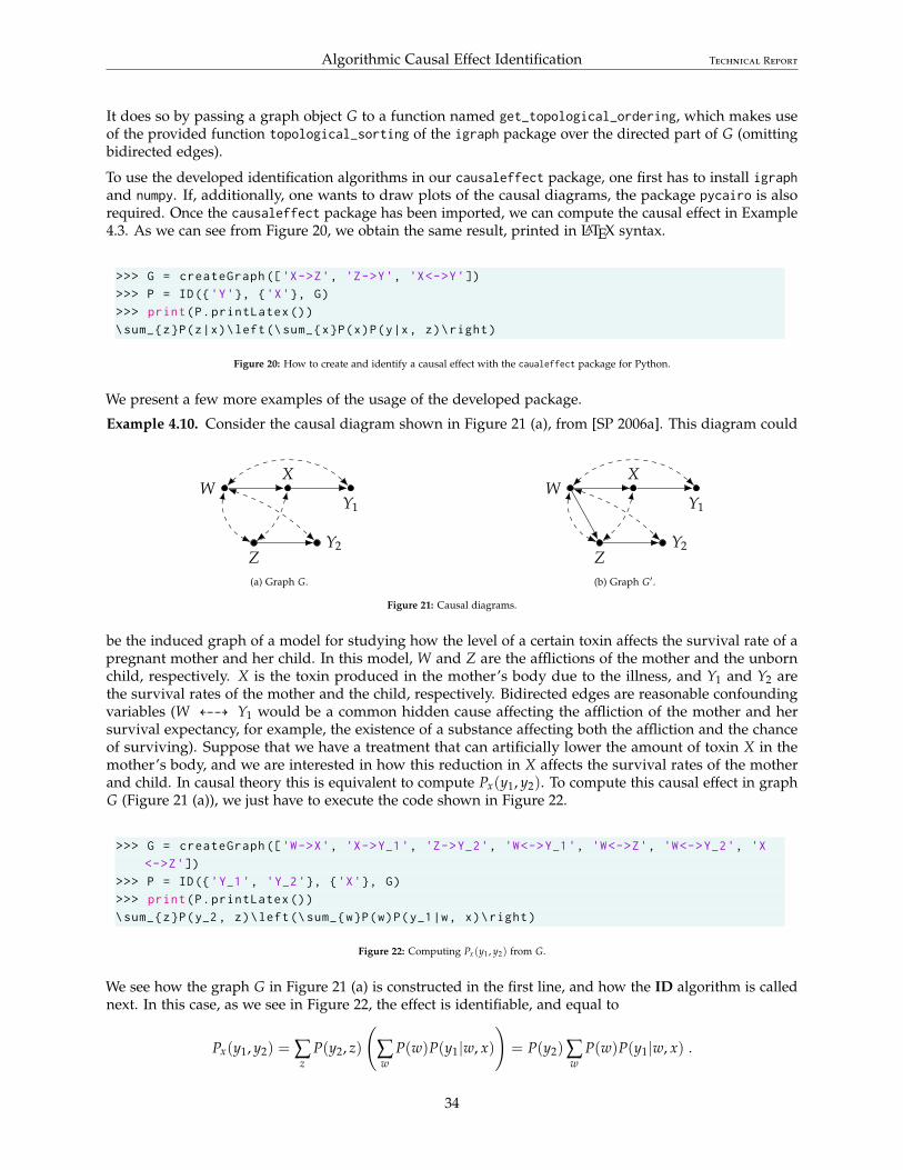
Algorithmic Causal Effect Identification Technical Report
It does so by passing a graph object G to a function named get_topological_ordering, which makes useof the provided function topological_sorting of the igraph package over the directed part of G (omittingbidirected edges).
To use the developed identification algorithms in our causaleffect package, one first has to install igraphand numpy. If, additionally, one wants to draw plots of the causal diagrams, the package pycairo is alsorequired. Once the causaleffect package has been imported, we can compute the causal effect in Example4.3. As we can see from Figure 20, we obtain the same result, printed in LATEX syntax.
>>> G = createGraph (['X->Z', 'Z->Y', 'X<->Y'])
>>> P = ID({'Y'}, {'X'}, G)
>>> print(P.printLatex ())
\sum_{z}P(z|x)\left(\sum_{x}P(x)P(y|x, z)\right)
Figure 20: How to create and identify a causal effect with the caualeffect package for Python.
We present a few more examples of the usage of the developed package.
Example 4.10. Consider the causal diagram shown in Figure 21 (a), from [SP 2006a]. This diagram could
WX
Y1
ZY2
(a) Graph G.
WX
Y1
ZY2
(b) Graph G′ .
Figure 21: Causal diagrams.
be the induced graph of a model for studying how the level of a certain toxin affects the survival rate of apregnant mother and her child. In this model, W and Z are the afflictions of the mother and the unbornchild, respectively. X is the toxin produced in the mother’s body due to the illness, and Y1 and Y2 arethe survival rates of the mother and the child, respectively. Bidirected edges are reasonable confoundingvariables (W 99KL99 Y1 would be a common hidden cause affecting the affliction of the mother and hersurvival expectancy, for example, the existence of a substance affecting both the affliction and the chanceof surviving). Suppose that we have a treatment that can artificially lower the amount of toxin X in themother’s body, and we are interested in how this reduction in X affects the survival rates of the motherand child. In causal theory this is equivalent to compute Px(y1, y2). To compute this causal effect in graphG (Figure 21 (a)), we just have to execute the code shown in Figure 22.
>>> G = createGraph (['W->X', 'X->Y_1', 'Z->Y_2', 'W<->Y_1', 'W<->Z', 'W<->Y_2', 'X
<->Z'])
>>> P = ID({'Y_1', 'Y_2'}, {'X'}, G)
>>> print(P.printLatex ())
\sum_{z}P(y_2 , z)\left(\sum_{w}P(w)P(y_1|w, x)\right)
Figure 22: Computing Px(y1, y2) from G.
We see how the graph G in Figure 21 (a) is constructed in the first line, and how the ID algorithm is callednext. In this case, as we see in Figure 22, the effect is identifiable, and equal to
Px(y1, y2) = ∑z
P(y2, z)
(∑w
P(w)P(y1|w, x)
)= P(y2)∑
wP(w)P(y1|w, x) .
34

Algorithmic Causal Effect Identification Technical Report
This means that we can actually know how this variation in X would affect Y1 and Y2 without having toperform the potentially hazardous treatment in real patients.
Suppose now that our model is slightly changed due to recent studies that suggest that the affliction ofthe mother directly influences that of the child. Taking this new information into account in our causaldiagram means adding one more edge, W → Z (see Figure 21 (b)). If we now try to identify the samecausal effect Px(y1, y2) in this new causal diagram G′ we will fail due to the existence of a hedge, as it canbe seen in Figure 23.
>>> G = createGraph (['W->X', 'X->Y_1', 'Z->Y_2', 'W<->Y_1', 'W<->Z', 'W<->Y_2', 'X
<->Z', 'W->Z'])
>>> P = ID({'Y_1', 'Y_2'}, {'X'}, G)
HedgeFound: Causal effect not identifiable. A hedge has been found:
C-Forest 1:
Vertices: W, X, Y_1 , Z, Y_2
Edges: W->X, X->Y_1 , Z->Y_2 , W->Z, W<->Z, W<->Y_1 , X<->Z, W<->Y_2
C-Forest 2:
Vertices: W, Y_1 , Z, Y_2
Edges: W->Z, Z->Y_2 , W<->Z, W<->Y_1 , W<->Y_2
Figure 23: Trying to identify Px(y1, y2) from G′ .
Indeed, we see that the first C-forest found by the algorithm is G′ itself, which has roots {Y1, Y2}. Moreover,we have {Y1, Y2} ⊂ An({Y1, Y2})GX
and {X} ∩ G′ 6= ∅. The other {Y1, Y2}-rooted C-forest is G′[V \ X],
which trivially fulfils {X} ∩ G′[V \ X] = ∅ and also G′[V \ X] ⊆ G′. Hence G′ and G′[V \X] form a hedgefor Px(y1, y2) in G′, making this causal effect unidentifiable.
Consider now this following example of a conditional causal effect computation.
Example 4.11. Imagine we want to compute the causal effect Px(y|z) in the causal diagram G presented inFigure 24. If we execute the code in Figure 25 (a), we retrieve the desired conditional causal effect,
Z
W
Y
X
Figure 24: Causal diagram G.
Px(y|z) = ∑x P(x|w)P(y|w, x, z)∑x,y P(x|w)P(y|w, x, z)
.
Observe that, although our package is able to simplify a handful of expressions, the obtained result can befurther reduced:
Px(y|z) = ∑x P(x|w)P(y|w, x, z)∑x,y P(x|w)P(y|w, x, z)
=∑x P(x|w)P(y|w, x, z)
∑x P(x|w)∑y P(y|w, x, z)= ∑
xP(x|w)P(y|w, x, z) .
This expression is interesting, since we do not fix nor condition on the variable W, and yet it appears in thefinal expression as a free variable (meaning it is not summed over all its possible values). In fact, despite
35

Algorithmic Causal Effect Identification Technical Report
>>> G = createGraph (['X<->Y', 'Z->Y', 'X->Z', 'W->X', 'W->Z'])
>>> P = ID({'Y'}, {'X'}, G, cond={'Z'})
>>> print(P.printLatex ())
\frac{\sum_{x}P(x|w)P(y|w, x, z)}{\ sum_{x, y}P(x|w)P(y|w, x, z)}
(a) Computing Px(y|z) from G in Figure 24.
>>> G = createGraph (['X<->Y', 'Z->Y', 'X->Z', 'W->X', 'W->Z'])
>>> P = ID({'Y'}, {'X'}, G)
>>> print(P.printLatex ())
\sum_{w, z}P(w)P(z|w, x)\left(\sum_{x}P(x|w)P(y|w, x, z)\right)
(b) Computing Px(y) from G in Figure 24.
Figure 25: Computing two causal effects with the implemented package.
appearing in the computed causal effect, said effect is independent of the value w, but in a practical settingsome value within the domain of W must be chosen for w. The independence can be easily seen fromFigure 24, because when intervening X and conditioning on Z we d-separate Y and W, thus making themindependent.
If we now want to compute the causal effect Px(y) in the same causal diagram G, we just slightly changethe call to the ID function, as we see in Figure 25 (b), and we obtain
Px(y) = ∑w,z
P(w)P(z|w, x)
(∑x
P(x|w)P(y|w, x, z)
),
which cannot be further simplified.
Consider the following example, from the causal model and data in Example 3.18.
Example 4.12. In Example 3.18 we had a causal diagram that modelled the probability of wearing sunscreendepending on the season and on the weather of that particular day. We want to see if a sunny day causes towear sunscreen, and to do so we will compute P(y) and Px(y) and compare them. First of all, we need tocalculate an expression for the interventional distribution, and we do it with our causaleffect package, asin Figure 26.
>>> G = createGraph (['Z->X', 'Z->Y', 'X->Y'])
>>> P = ID({'Y'}, {'X'}, G)
>>> print(P.printLatex ())
\sum_{z}P(y|x, z)P(z)
Figure 26: Creation of graph G from Example 3.18 and computation of Px(y) from G.
We have obtained Px(y) = ∑z P(y|x, z)P(z), which is exactly the Back-Door Adjustment (note that Z fulfilsthe back-door criterion relative to (X, Y)). Now we will compute these probabilities from data in Table 3,but to do so we need to remember that we did not have P(X, Y, Z), but instead the conditional probabilities:P(X, Y, Z) = P(Y|X, Z)P(X|Z)P(Z). We first compute what is the probability of wearing sunscreen.
P(Y = T) = ∑x,z∈{T,F}
P(X = x, Y = T, Z = z)
= ∑x,z∈{T,F}
P(Y = T|X = x, Z = z)P(X = x|Z = z)P(Z = z)
= 0.99 · 0.90 · 0.25 + 0.20 · 0.70 · 0.75 + 0.60 · 0.10 · 0.25 + 0.05 · 0.30 · 0.75= 0.354 .
36
Algorithmic Causal Effect Identification Technical Report
Then, we compute the probability of wearing sunscreen imposing that it is sunny. This intervention cannotbe done in real life, and that is the beauty of it!
P(Y = T|do(X = T)) = ∑z∈{T,F}
P(Y = T|X = T, Z = z)P(Z = z)
= 0.99 · 0.25 + 0.20 · 0.75= 0.3975 .
To compare even more results, we also compute the probability of wearing sunscreen given that we see it issunny.
P(Y = T|X = T) =∑z∈{T,F} P(X = T, Y = T, Z = z)
∑y,z∈{T,F} P(X = T, Y = y, Z = z)
=∑z∈{T,F} P(Y = T|X = T, Z = z)P(X = T|Z = z)P(Z = z)
∑y,z∈{T,F} P(Y = y|X = T, Z = z)P(X = T|Z = z)P(Z = z)
=∑z∈{T,F} P(Y = T|X = T, Z = z)P(X = T|Z = z)P(Z = z)
∑z∈{T,F} P(X = T|Z = z)P(Z = z)
=0.99 · 0.90 · 0.25 + 0.20 · 0.70 · 0.75
0.90 · 0.25 + 0.70 · 0.75=
0.327750.75
= 0.437 .
We see that P(Y = T|do(X = T)) > P(Y = T), and this rise in probability reveals that the sun causes towear sunscreen. Additionally, we also see that the conditional probability is bigger than the interventional,P(Y = T|X = T) > P(Y = T|do(X = T)). We believe that the probability of wearing sunscreen increasesmore when we see it is sunny than when we force it to be sunny because when it is sunny it is also morelikely to be summer, and this also affects the probability of wearing sunscreen. On the other hand, whenwe intervene to be sunny it does not care if it is summer or not.
4.4 From Causal Effects to Counterfactual Queries
We have already seen how, using causal diagrams and the do-operator, we can answer causal queries fromthe second level of the Ladder of Causation when they are identifiable. The next natural step would be tostudy and formalize the concept of counterfactuals, and try to build a technique to answer counterfactualquestions from observational data. This journey was undertaken by none other than Shpitser and Pearl[SP 2007], authors of the previous algorithms for computing causal effects. In this section, we will brieflyexplain an idea of their work regarding the identifiability of counterfactual queries and some algorithmsmade to evaluate them, although we have not implemented those in our package as they were far toocomplex and out of the scope of this project.
To be able to answer counterfactual queries, the authors introduced some notation. The reader can referto [Pea 2000] for an extensive discussion on counterfactuals and the notation used. A variable Y affectedby an intervention do(x) is changed into a counterfactual variable, and it is denoted by Yx. Then, questionssuch as “what if X were x” would be represented as P(Yx|e), where e are observations that induce theprobability distribution. There is an intrinsic problem with these types of queries and it is that actions xand evidence e can stand in logical contradiction, and no experimental setup exists which would emulateboth the evidence and actions. For instance, there is no experiment that allows us to know the percentageof deaths that could be avoided among people who received a given treatment, had they not taken thetreatment. So it is unclear if counterfactual expressions like P(Yx|e), with e and x incompatible, can beestimated consistently.
The authors designed two algorithms [SP 2007] to identify counterfactuals and evaluate them from inter-ventional probabilities when identifiable. To do so, they introduce the concept of parallel world graphs, whichcan be thought as multiple causal diagrams (each one of them representing a possible world, with a precise
37

Algorithmic Causal Effect Identification Technical Report
X D
W Z
Y
U
(a)
X D
W Z
Y
U
U
Uw
Uz
Ud
Dx
WxZx
Yx
Xd
WdZd
Yd
(b)
Figure 27: (a) Causal graph G of model M. (b) Parallel world graph of G for P(yx |x′ , zd , d), formed by three worlds: the original model M (centre,green) and the submodels Mx (left, red) and Md (right, blue).
intervention) sharing the same exogenous variables. An example of a parallel world graph taken from[SP 2007] is shown in Figure 27.
Figure 27 (a) is the induced causal graph G of the causal model M. M models how drugs X and D affectintermediate symptoms W and Z, which in turn influence another symptom Y. Suppose that we want toknow how likely the patient would be to have a symptom Y given a certain dose x of drug X, assumingwe know that the patient has taken dose x′ of drug X, dose d of drug D, and we also know how theintermediate symptom Z responds to treatment d. This causal query can be expressed as P(yx|x′, zd, d), andthe parallel world graph would be formed by three worlds: the original model M and also the submodelsMx and Md, as seen in Figure 27 (b). Note that we have not included nodes fixed by actions in the parallelworld graph since we already know their values, which are constant.
Parallel world graphs can have duplicate nodes (for instance, in Figure 27 (b) we have Z = Zx since Z isnot a descendant of X), and this could arise some errors when computing d-separation. So what they dois they merge duplicate nodes following rigorous criteria and create what they call counterfactual graphs,which is equivalent to counterfactual queries as a causal graph is to causal queries.
They present two algorithms similar to the ones for causal queries, called ID∗ (for unconditional queries) andIDC∗ (for conditional queries), that given a causal graph and a counterfactual query return either an error oran expression for computing the counterfactual query from interventional probabilities. Analogously to thecausal case, they are recursive, and IDC∗ calls ID∗ as a subroutine. They have to work with counterfactualgraphs, so they construct them from the inputted causal graphs using another algorithm also defined inthe paper, named make-cg. Note that both ID∗ and IDC∗ return interventional probabilities, so to finallyobtain results from observational data one has to use the causal effect algorithms already defined in thissection.
The implementation of these counterfactual identifying algorithms is highly non-trivial and would requirethe construction of additional classes and functions.
5 Conclusions
Causal theory is a field in statistics that until recently had not been studied much. The influence of powerfulstatisticians, like Karl Pearson, discouraged the use of causal graphs to compute causal queries in thefirst half of the twentieth century, but in the last thirty years, thanks to Pearl and many other scientists, aformalized causal theory has been built.
38
Algorithmic Causal Effect Identification Technical Report
This mathematization of causal questions reached a peak with the design of deterministic algorithms thatidentify and, when possible, compute causal effects from observational data. Although known by manyscientists, these results are unknown to many others, and to bring them to a wider audience the author hasimplemented a new Python library that computes causal effects. This package is very practical since inonly two lines of code one can construct a causal graph and query a causal effect.
This is not the first developed package with these results. To the best of the author’s knowledge, the onlyimplementation of these identification algorithms before the one presented in this work is the R packagecalled causaleffect, by Tikka and Karvanen [TK 2017]. In this project, the author has also studied inutmost detail this package and its associated paper and has found a subtle bug in the implementation ofIDC. This error was reported to the authors, and it has already been fixed in version 1.3.13 (June 14th, 2021).
The implementation and analysis of the identification algorithms presented in this work have required theauthor to go through the necessary background mathematical results on the theories involved. I believethis has been vital to present the results in this work in a more organized and clearer way, and I expect thisto be a gateway for more scientists to discover Pearl’s remarkable results.
As the author has stated in this work, a logical extension of this project would involve the implementationof counterfactual identification algorithms. To do so, one would have to sail through the obscure notationof counterfactual formalization. If successful, this would finally enable the computation of counterfactualqueries, questions of the third level of the Ladder of Causation.
6 Source Code
The source code of the developed Python library, causaleffect, can be found in the following GitHubrepository:
https://github.com/pedemonte96/causaleffect
Every figure containing code in this work has its equivalent Python script in the provided repository.
References
[Ash 1970] Ash, R. B. (1970). Basic probability theory. Wiley New York.
[BLW 1986] Biggs, N., Lloyd, E. K. and Wilson, R. J. (1986). Graph Theory, 1736-1936. Clarendon Press.
[Pea 1993] Pearl, J. (1993). Comment: graphical models, causality and intervention. Stat. Sci. 8 (3) pp.266-269.
[Pea 1995] Pearl, J. (1995). Causal Diagrams for Empirical Research. Biometrika 82 (4) pp. 669-688.
[Pea 2000] Pearl, J. (2000). Causality: Models, Reasoning, and Inference. Cambridge University Press.
[PGJ 2016] Pearl, J., Glymour, M. and Jewell, N. P. (2016). Causal inference in statistics: a primer. WileyChichester.
[PM 2018] Pearl, J. and Mackenzie, D. (2018). The Book of Why. Penguin Random House UK.
[SP 2006a] Shpitser, I. and Pearl, J. (2006). Identification of Joint Interventional Distributions in RecursiveSemi-Markovian Causal Models. AAAI Press. pp. 1219-1226.
[SP 2006b] Shpitser, I. and Pearl, J. (2006). Identification of Conditional Interventional Distributions. AUAIPress. pp. 437-444.
[SP 2007] Shpitser, I. and Pearl, J. (2007). What Counterfactuals Can Be Tested. AUAI Press. pp. 352–359.
[Tian 2002] Tian, J. (2002). Studies in Causal Reasoning and Learning. PhD Dissertation, Department ofComputer Science, University of California.
[TIOBE 2021] TIOBE Software BV (2021). TIOBE Index for June 2021. https://www.tiobe.com/tiobe-index/.
[TK 2017] Tikka S. and Karvanen J. (2017). Identifying Causal Effects with the R Package causaleffect. J.Stat. Softw. 76 (12) pp. 1-30.
39

Algorithmic Causal Effect Identification Technical Report
[Ver 1993] Verma, T. S. (1993). Graphical Aspects of Causal Models. UCLA Cognitive Systems Laboratory,Technical Report (R-191).
[VP 1988] Verma, T. S. and Pearl, J. (1988). Causal Networks: Semantics and Expressiveness. UAI.
40