Working Papers No. 163/12

Reparations, Deficits, and Debt Default: The

Great Depression in Germany

Albrecht Ritschl

© Albrecht Ritschl

June 2012

Department of Economic History

London School of Economics

Houghton Street

London, WC2A 2AE

Tel: +44 (0) 20 7955 7860

Fax: +44 (0) 20 7955 7730

1

Reparations, Deficits, and Debt Default: The Great Depression in Germany

Albrecht Ritschl

ABSTRACT

Germany’s Great Depression of the early 1930s started in 1929 with a sudden stop in the

current account. It ended after a foreign debt default that unfolded in several stages from 1931 to

1933. This chapter reviews Germany’s macroeconomic history between the gold-based stabilisation

of 1924 and the transition to autarky and domestic credit expansion in 1933. During the Dawes

Plan of 1924-29, German borrowed abroad massively to pay reparations out of credit, a

phenomenon that gave rise to the debate about the transfer problem between Keynes and his

critics. An incentive based interpretation of the transfer problem is sketched to explain the later

current account reversal. Time-varying VARs are employed to trace the propagation of the resulting

macroeconomic shock, and to obtain estimates of fiscal multipliers.

Chapter prepared for: Nicholas Crafts and Peter Fearon (eds.) The Great Depression of the 1930s: Lessons for Today, Oxford: Oxford University Press.

2

1. Introduction

Plagued by structural unemployment throughout the 1920s, the German economy went

through a sharp contraction after 1929, followed by complete recovery and the restoration of full

employment around 1937. Both the timing and the severity of the contraction set Germany apart

from European developments at the time, bearing similarities to the U.S. depression instead. Like the

U.S., Germany experienced a strong economic rebound between 1933 and 1936, surpassing growth

rates in most European countries. In a significant departure from the U.S. pattern, however,

Germany’s recovery continued after that year, joining the economies of Northwestern Europe in

avoiding the recession of 1937/38 (see Feinstein, Temin and Toniolo, 1997).

Between the return to the Gold Standard in 1924 and the beginning of World War II, the

German economy went through a succession of reparation arrangements, which coincided with

balance of payment regimes. These were characterised by increasingly tight foreign borrowing

constraints and growing levels of debt default. Germany went from being a massive capital importer

during the Dawes Plan of 1924-29 to a sudden stop in its current account under the Young Plan of

1929/30, and on to an autarkic command economy with tight capital and foreign exchange controls

after the end of the Young Plan in 1932. The timing of these regime switches coincided with the

turning points of the German business cycle and defined the limits and scope for domestic

macroeconomic policies.

This chapter reviews Germany’s macroeconomic performance between 1924 and 1938 with a

view to the reversals in its international payments position and their consequences. The main

observation is that the quick succession of reparation arrangements, each with its own incentive

problems and borrowing constraints, created distinct macroeconomic policy regimes. After the gold-

based stabilisation under the Dawes Plan of 1924 and a short-lived adjustment crisis, Germany

experienced recovery led by large short-term capital inflows. This enabled Germany to pay reparations

on credit – an effect soon named the transfer problem, which had been predicted by Keynes and

which was discussed controversially with his critics at the time (Keynes, 1922; 1929; Ohlin, 1929). The

same capital inflows also allowed Germany to maintain large current account deficits. With monetary

policy largely constrained by the Gold Standard, fiscal policy adopted a neutral stance. While it

avoided major deficits, it also failed to generate the surpluses needed to effect reparation transfers, a

fact which Keynes’ detractors were quick to point out (see Rueff, 1929; Mantoux, 1946). With tighter

terms of reparation payments looming under the Young Plan and a substantial amount of

accumulated foreign debt, Germany experienced a sudden current reversal in early 1929,

accompanied by the first of a series of public debt funding crises. As a consequence, fiscal policy

switched to austerity and forced deflation in the summer of 1929. This change came at the hand of

3

the Reichsbank, Germany’s central bank that had been made independent of the government in 1922

and put under international control in 1924. Violating the letter but arguably not the spirit of its

statutory rules, the Reichbank in mid-1929 began offering short-term credit to the government but

imposed a programme of severe budget cuts, which was adhered to through 1931. The open

outbreak of the budget crisis was delayed through an international stabilization loan in connection

with the Young Plan, which however imposed similar conditions on fiscal policy (see Ritschl, 2002).

At the core of the analysis of this chapter is an incentive-based interpretation of the German

transfer problem under the Dawes Plan. Political scientists and diplomatic historians have long agreed

that the foreign exchange arrangements under Dawes Plan gave Germany an incentive to borrow

abroad excessively, with a view to driving out reparations in a future transfer crisis (see Helbich, 1962;

Link, 1970; McNeil, 1986; Schuker, 1988). This mainstream argues that the Young Plan with its

tighter terms of payment was a response to this incentive problem. As a consequence, the sudden

stop in Germany’s current account after 1928 was endogenous to Germany’s debt levels, restoring an

external credit constraint on the German economy that the Dawes Plan had temporarily softened (see

the discussion in Ritschl, 2002).

Historians have been in bitter controversies about alternatives to Germany’s fiscal policy during

the slump since Borchardt’s (1979) claim that the government faced a borrowing constraint (see the

opposing views in Borchardt, 1990; Holtfrerich, 1990; as well as the restatement of the traditional

position in Ferguson and Temin, 2003). The austerity policy pursued seems easier to motivate and

explain with reference to Germany’s mounting foreign debt problems (Ritschl, 2002). Accounting for

the foreign dimension of Germany’s debt problem - notably, the reparations issue – also sharpens the

focus on policy counterfactuals and their historical feasibility.

Germany’s debt crisis and recovery holds a series of lessons in stock for today’s attempts to deal

with high levels of national debt. The central bank’s conditioning of debt monetisation on a

government austerity programme resembles current attempts to reign in the fiscal policy of debtor

countries in the Eurozone. Then as now it depends for its success on the willingness of other creditors

to fall in line, and at the same time is a test of the central bank’s own anti-inflationary credibility.

The rest of this chapter is structured as follows. Section 2 provides a brief survey of Germany’s

reparations arrangements, in particular the Dawes and Young Plans. The subsequent sections examine

the macroeconomic regimes associated with these plans for key macroeconomic variables, with

Section 3 looking at monetary policy, Section 4 focussing on fiscal policy, and Section 5 turning to

labour demand and investment. Section 6 concludes with implications for the Great Recession after

2008.

4

2. Germany’s Reparation arrangements: a brief refresher

German reparations after World War I were not fixed immediately. The peace conference in

Paris ended with compromise formulae on this matter, however without reaching consensus among

the Allies on how much to demand from the Germans. The two main building blocks of any

reparations were supposed to be indemnities proper, as well as compensation for inter-allied World

War I debts. The main instruments of reparation payment were to be confiscation of overseas assets,

deliveries out of existing stock, deliveries in kind out of current production, and monetary payments in

gold-based foreign exchange. Issuing reparations bonds and floating them on international markets,

as France had done with her reparations to Prussia after the war of 1870/1, was considered briefly but

discarded. Nevertheless, the concept of denominating reparations in bonds was retained even if

flotation in the markets was seen as difficult given the magnitudes involved. During an interim period

until the final bill was drawn up, payment consisted largely in confiscations of physical and intellectual

property abroad, as well as in deliveries in kind.

Reparations soon came to be seen as odious by much of academia, and indeed by considerable

parts of the public. Confronted with rather unrealistic figures on planned reparations, Keynes pulled

out in protest from his role as an advisor to the British delegation in Paris and published his scathing

criticism in his Economic Consequences of the Peace (Keynes, 1920). Keynes’ approach to the issue

provided the framework for most of the future discussion, shaping the views even of his critics. He

argued that the envisaged reparations would exceed Germany’s capacity to pay, and if ever seriously

enforced would cause widespread economic disruption, even famine, and ultimately the rise of a

dictatorship bent on waging a war of revenge. In later work, Keynes added that reparation transfers

would be near-impossible to effect, due to both protectionism in the recipient countries and the

difficulties of lowering German wages sufficiently. And if attempted, transfers would be counteracted

by capital inflows (on this and the ensuing controversy see Keynes, 1926; 1929; Ohlin, 1929; Rueff,

1929). The transfer problem in the presence of high capital mobility soon became a standard fixture

of open economy macroeconomics (Metzler, 1942; Johnson, 1956).

Reparations as determined by the London ultimatum of 1921 came in three tranches, a net

indemnity of 12 bn gold marks (A bonds), a compensation of 38 bn gold marks for inter-allied war

debts (B bonds), and an additional, largely notional charge of 82 bn gold marks (C bonds). Depending

on which part of these reparations is included, a wide range of debt-to-GNP ratios can be obtained

(See Table 2.1).

5

Legally, all three tranches of the 1921 reparations bill were owed, although there is wide

consensus that the largest bit, the 82 bn gold marks of C bonds, was mostly a political bargaining

chip and essentially served for domestic policy purposes in London and Paris (Feldman, 1993).

Taken in isolation, the A bonds amounted to 20% of German GDP of 1913, a burden that was

equivalent to France’s reparations to Germany in 1871 (Ritschl, 1996). Adding the B bonds generated

a reparations burden of 100% of 1913 GDP. Including also the C bonds raised the reparations burden

to over 260% of 1913 GDP. However, it was communicated to the Germans that the C bonds would

not have to be paid under any realistic conditions. The Germans had anticipated a burden of 30-40bn

gold marks. Hence, the realistic part of the reparation bill was not entirely beyond the imagination of

German policy makers (Feldman, 1993; Ferguson, 1998).

News of the reparations bill nevertheless proved toxic for Germany’s nascent Weimar Republic.

Weimar’s new constitution of 1920 had strengthened and centralized tax collection with a view to

generating a strong tax base. Tax revenues under the news system initially looked promising and

brought post-war inflation to a temporary halt (Dornbusch, 1987). However, when news broke in late

1920 that reparations might be far higher than expected by the German public, a veritable tax

boycott developed. Tax collection plummeted, the monetization of short term government paper

resumed, and inflation accelerated again. In a confrontational climate, the finance minister and

architect of Weimar’s fiscal constitution, Erzberger, was forced to resign and was later assassinated.

The government adopted a progressively less cooperative stance vis-a-vis reparations, provoking the

French occupation of the Ruhr district in late 1922. A policy of passive resistance against the occupiers

was proclaimed, leading to a significant drop in German output, combined with ever-higher

hyperinflation in 1923.

Stabilization of the German currency in late 1923 was part of a political settlement that

included reparations. Under the Dawes Plan of 1924, reparations were rescheduled but not formally

reduced. To assist in the recovery of the German economy, reparation annuities were phased in

gradually from a low base to reach a steady state in 1929. Discounted at 5%, the interest rate of the

Dawes loan, they amounted to 42bn reichsmarks in present value in 1924, slightly below the sum of

A and B bonds fixed in the London ultimatum. The resulting debt/GDP ratio for 1925 was 68%,

marginally down from the 70% debt/GDP ratio implied by the sum of A and B bonds. The ominous C

bonds were left out of the Dawes Plan but were formally not off the table.

A burden this size was by no means impossible to bear. There is broad consensus on this issue

both internationally (see e.g. Marsh, 1998, Ferguson, 1998) and east of the Rhine (Hardach, 1980;

Holtfrerich, 1986; Ritschl, 1996). However, while France’s and Britain’s debts were largely

denominated in domestic currency, Germany’s reparation burden was owed in foreign currency and

6

to foreign claimants, giving rise to Original Sin (Eichengreen and Hausman, 1999). The sovereign

nature of German reparation debt implied willingness-to-pay constraints (see Eaton, Gersovitz and

Stiglitz, 1986), which should potentially limit the amount of credit to be obtained from foreign

lenders.

Given these debt constraints, Germany’s balance of payments during the mid-1920s presents a

paradox: on the one hand, the country owed heavy reparations. On the other, it was able to attract

major capital inflows. This evidence seems contradictory, and the capital inflows of the 1920s are

indeed at the root of a debt crisis. This crisis would break out in full during the Great Depression and

culminate in near-complete debt default in 1933 (Klug, 1993).

Indeed, the debt burden implied by the Dawes Plan was higher than just the present value of

the Dawes Plan annuities themselves. While excluded from the Dawes Plan payment scheme, the

ominous C bonds had not been formally rescinded and still loomed as a risk, all the more so as

reparations were a first charge on Germany under the peace treaty. Including the C bonds, the

reparations total under the Dawes Plan amounted to 180% of German GDP in 1925. This makes it

less than straightforward that Germany was able to attract foreign credit in significant measure after

1924. Even ignoring the C bonds, the Dawes Plan’s 68% charge on Germany’s 1925 GDP left only

limited room for foreign credit if a sovereign debt crisis was to be avoided.

However, the Dawes Plan created a loophole by giving commercial claims on Germany transfer

protection against reparations. Transfer protection implied that at the central bank’s foreign exchange

window, transfers of dividends and interest on commercial loans would take precedence over

transfers of reparations. This had the effect of making reparation recipients the residual claimants on

German foreign exchange surpluses. While not repudiating the peace treaty’s principle that

reparations were first rank, transfer protection for commercial claims reversed seniority in terms of

foreign exchange. Thus, reparations were effectively turned into junior debt. (Ritschl, 1996; 2002).

This created a double moral hazard problem. With reparations effectively being of lower rank,

the German government had little incentive during the Dawes Plan to stem the inflow of foreign

credit. On the contrary, the more funds came in, the less would have to be paid out in reparations.

This logic was understood and widely accepted in German government circles. Already in 1924, a

memorandum in Germany’s Foreign office pointed out that foreign debt would turn Germany’s

commercial creditors into hostages of future editions of the reparations conflict (Link, 1970; McNeil,

1986). Opposition came only from the Reichsbank, which was worried that paying reparations on

credit would only perpetuate the reparations conflict. If a crisis of reparations was inevitable, it was

preferable to have it sooner than later, before Germany’s foreign creditworthiness was irreversibly

damaged (James, 1985).

7

Moral hazard existed also on the part of commercial creditors. As long as Germany’s

commercial debt was small relative to her gains from trade (the ultimate measure of her willingness to

continue participating in international credit markets), lending seemed perfectly safe, even if it has the

effect of crowding out reparations at the margin. Only if the level of commercial debt threatened to

approach the willingness to pay constraint (or alternatively, if transfer protection was only imperfectly

credible) did commercial creditors have an incentive to take a closer look before the signed up.

Matters were not helped by the fact that the Dawes Plasn itself was drawn up by New York bankers

(Schuker, 1976).

Transfer protection proved quite effective in attracting foreign credit, and created a distinct

macroeconomic regime. In all years of the Dawes Plan, the current account was negative, implying

that Germany borrowed more than needed to recycle reparations. (See Table 2.2)

The current account deficits indeed exceeded reparations in most years; reparations thus only

played a secondary role in the built-up of foreign debt. Up until 1928, reparation payments were

roughly matched by long term capital imports. On balance, the current account deficit was financed

with short term capital imports.

This caused concern both among reparation claimants and, once debt levels were high enough,

among commercial creditors. An Agent General for Reparations, located in Berlin to monitor German

compliance with the Dawes plan, lobbied against German foreign borrowing. With arguments similar

to the Reichsbank, his reports urged that capital inflows into Germany must be stopped and

suggested that withdrawing transfer protection of the returns on these investments would be the way

forward (Gilbert, 1925-30). However, 1928 was an election year in the U.S., France, and Germany,

and as transfer crisis was seen as the likely outcome of this change, no decisions were taken.

Negotiations over a new reparations deal with tighter terms of payment began in late 1928.

The German side hoped that in return for abandoning transfer protection, it could achieve

considerably lower annuities. On the Allied side, the stabilization of the Franc in 1928 and the

Bérenger/Mellon accord on the resumption of French debt service on inter-allied war credits aligned

the incentives of U.S. and French policy makers and resulted in a hardened position. The new plan

envisaged reparations equivalent to the remaining inter-allied war credits still owed to the US by

France and Britain. The scheme was deemed final, which removed the remaining uncertainty about

the C bonds.

News on this was leaked in March 1929. Under the new scheme, commercial transfers would

only be protected for up to one year, after which reparation transfers would regain seniority.

Reparation annuities were to decrease only marginally, but a new stabilization loan was to be floated

8

once the plan was ratified. The immediate effect of the news leak was a first confidence crisis in

money and bond markets in the same month. The central bank lost reserves; a central government

bond flotation failed, and a sudden stop in long-term capital inflows ensued: net capital long-term

imports in 1929 declined by 75% from the previous year. Commercial debt alone now equalled 30%

of GDP; about two thirds of that debt was short term. Including reparations, total foreign debt would

reach 80% of GDP in 1929, or 75% under the reduced Young Plan annuities if Germany accepted

the new plan. The offer included a full withdrawal of French troops from the remaining territories

occupied in 1923, as well as an end to international control over the railway system. This and a

threatening budget squeeze induced Germany to accept the Young Plan, despite the risk of being cut

off from international capital markets. (See Table 2.3)

Transition to the Young Plan brought about major political change in Germany. Within a year

from the March 1929 crisis, the finance minister, his budget director, the Reichsbank’s president, and

finally the government itself were out of office. A government of technocrats was appointed and the

country ruled by presidential emergency decree, activating the same reserve constitution that had

been employed in preparation of currency stabilisation during 1923. Political historians tend to agree

that this transition marked the end of Weimar as a democracy, almost three years before its final

demise.

The stabilisation loan floated in 1930 temporarily alleviated the pressure and postponed the

current account reversal until 1931. The data in Table 2.2 show that in the commercial long-term

market, Germany became a capital exporter, losing long-term loans for the first time since the

stabilisation of 1924. With national output in decline, the ratio of foreign debt to national income

increased quickly. Failure to win parliamentary approval for the 1930 austerity budget brought about

parliamentary elections in September 1930, which saw the extreme right and left increase their

combined vote to almost 40%. Foreign credit to the central government after that date was not

forthcoming, and further fiscal tightening ensued.

German politics found itself caught between increasing domestic pressure to unilaterally

default on the Young Plan and international demands to stay current on her payments if a return to

sanctions or military action was to be avoided. By spring 1931, the ratio of foreign debt to GDP

approached 100%, and reserve losses accelerated after an Austro-German customs union project

failed under foreign pressure, prompting the resignation of the Austrian government and coinciding

with the near-collapse of Creditanstalt, Austria’s largest commercial bank (James, 1986).

Breaking away from an earlier commitment to fully comply with the Young Plan during its first

year, the German government in early June warned publicly it might not be able to fully transfer both

foreign debt service and reparations for the year. With this announcement, the issue of seniority of

9

reparations over commercial foreign debt was open again. A series of negotiations and an

international conference in the same month failed to produce clear results. While France was willing

to extend short term credit in exchange for foreign policy concessions from Germany, both Britain and

the U.S. were opposed, as injecting fresh money implied a return to recycling reparations through

credit.

Under heavy international pressure, Germany refrained from taking unilateral steps and would

neither declare default nor leave the Gold Standard. Instead, the moratorium proposed by U.S.

president Hoover introduced a one-year reparations holiday, combined with an offer to negotiate a

standstill on short term debt (see Schuker, 1988, for a detailed account). However, no fresh money

would be injected into the German economy this time, and no substantial central bank credit was

given to replenish Germany’s foreign exchange reserves. The price of this arrangement was a full-

fledged banking and payments crisis. Shaken by the fraudulent bankruptcy of a major industrial client,

DANAT, a major bank, became insolvent. In response to the banking crisis, credit restrictions were

imposed and bank holidays declared. In a rescue operation, four out of five of Germany’s largest

banks were recapitalised and placed under government control (Schnabel, 2004).

As a consequence of the 1931 crisis, the Young Plan was suspended though not yet gone.

Amidst negotiations about its future, Germany tightened her deflation policy further to demonstrate

willingness to pay, while an international commission investigated her capacity to pay. Published in

the Beneduce report of November 1931, its findings were that given the international slump,

reparations under the Young Plan should not be resumed (Toniolo, 2005). A political settlement was

delayed by parliamentary elections in France, as well as presidential elections in Germany due in the

spring of 1932. Reparations were cancelled in August 1932.

August 1932 marked the trough of the depression in Germany. In the following month, the

first steps were taken towards expanding domestic credit behind a firewall of foreign exchange

controls. However, these controls were still far from complete. For the time being, Germany remained

current on her foreign long-debt, while the short-term debt was rolled over in a process of continuous

renegotiations, with foreign creditors carefully monitoring every step of German credit policies (Klug,

1993).

Transition to full-fledged capital controls came only after Germany’s unilateral debt default in

May 1933, and even then with a delay. In a reversal of strategy, Germany now attempted to minimize

transfers on long-term debt while staying current and in cases resuming debt service on parts of her

short-term standstill debt, discriminating among trading partners. This uncooperative approach was

initially less than successful, and transfers increased again. A balance of payments crisis threatened in

10

1934 when credit expansion began in earnest. The response was the establishment of a state

monopoly on foreign exchange, which completed Germany’s foreign debt default.

3. The Reichsbank and the Effects of Monetary Policy

The various reparations plans translated themselves into distinct macroeconomic policy regimes.

Stabilization from the hyperinflation was seen by policy makers and contemporary observers as being

primarily a monetary task. Stabilization in late 1923 created new currency units, converted from the

inflated paper mark at 1012: 1. The new currency was initially based on gold-indexed mortgage

bonds and later linked to gold at the pre-war parity, however without revaluing most of the

outstanding public debt. To lend credibility to the stabilization, the Reichsbank was placed under

international supervision and received a set of strict rules, including a tight cap on lending to the

government. A 40 % gold cover for notes in circulation and deposits at the Reichsbank was

prescribed.

Even under this strict regime, monetary aggregates in the second half of the 1920s increased

faster than real output, making it plausible that the stabilisation from the hyperinflation was more

fiscal than monetary in nature (Sargent, 1982). The foreign credit boom under the Dawes Plan was

reflected by inflows of gold and currency reserves to the central bank. Eager to build up a buffer stock

of reserves, the Reichsbank partly sterilized these inflows but still allowed a substantial increase in the

monetary base. Owing to a rapid recovery in deposits, the quantity of money increased even faster;

real M1 grew by 40% in a matter of five years.

With its hands tied by the Gold Standard and the transfer protection clause, the central bank

relied on indirect means to make its influence felt. These included moral suasion, announcements and

repeated forays into the domain of fiscal policy. The Reichsbank in 1926 began a political campaign to

stem the inflow of foreign funds, lobbying in vain to be given control over the foreign borrowing of

states and municipalities. In May 1927 it threatened credit rationing in the money market if foreign

inflows did not recede. This and repeated warnings by the Reparations Agent about German

borrowing helped to cool off the mood of international investors, and both investment and the stock

market began a slow decline.

Having acted as a whistle-blower on German borrowing, the Reichsbank in late 1928 became

involved in the negotiations over a revised reparations package. The confidence crisis caused by the

news of March 1929 gave the Reichsbank sufficient leverage to influence fiscal policy. Under the

impression of the bad news on reparations, a major loan flotation planned for the the same month

11

failed, leaving government in a scramble for cash. In conflict with its statutes, the Reichsbank stepped

in and began providing short-term loans to the government, however under strict conditionality.

These conditions included a sharp turn towards deflationary policy, as well as the creation of a sinking

fund with senior claims to the government to ensure the reduction of short term government debt

according to a fixed schedule. Meeting these conditions and continuing debt service to this sinking

fund became the basic tenets of government policy until after the end of the Young Plan in 1932.

As output began to fall in mid-1929, monetary aggregates declined as well. GDP in 1930 was

7% below the 1929 level, and M1 declined by the same amount. Initially this decline was driven in

equal measure by a loss in deposits and gold reserves. Losses of reserves became massive in the run-

up to the crisis of summer 1931, outpacing the loss of deposits. Desperate attempts to secure

international central bank credit remained unsuccessful. The crisis grew into a banking panic, to which

the Reichsbank responded by imposing bank holidays, closing the stock exchanges and placing four of

five leading commercial banks under public control. At the same time, it reduced the gold cover to

20% and increased the monetary base to a level beyond the 1929 peak. However, further reserve

losses during the spring of 1932 and the attempt to defend the lower gold cover led to renewed

monetary contraction.

Monetary expansion only began in early 1933 when the Reichsbank suspended gold

convertibility. The gold parity was formally not abandoned but became increasingly meaningless as

foreign exchange controls were tightened progressively. A complex network of bilateral exchange

agreements with split exchange rates emerged during 1934. Designed primarily to complete the

foreign debt default and minimize its domestic consequences, the transition to foreign exchange

control resulted in an average devaluation of 30-40%.

Already during the gold standard, the Reichsbank relied on a network of public proxy banks to

carry out operations not within its own remit. These off-balance-sheet institutions would lend against

bills that did not meet the Reichsbank’s eligibility standards, and conducted open market and buyback

operations. This system of proxy institutions gained importance after 1931 and took a key role in

financing the public shadow budgets beginning in 1933. Plans had existed already in 1930 to use this

network to finance public borrowing in the money market, given that overt government borrowing

would lead to renewed reparation demands. Public banks would be used to accept bills of exchange

issued in conjunction with public works. These bills would be formally private and designed to meet

the eligibility criteria at the central bank’s discount window. Though formally created as three-monthly

paper, these bills carried prolongation coupons for up to five years. This gave investors the option

value of redeeming the bills at par quarterly horizons. The Reichsbank would receive short-term

treasury bills as collateral from the government. It was hoped that in this way, liquid money market

12

assets could be created that were attractive for private investors to hold and would not have to be

monetized at the central bank. These plans did not materialize before the end of 1932; an attempt by

the Bruening government to finance a first wave of work creation in this way in the spring of 1932 –

when international, notably French opposition to domestic credit expansion in Germany was

considerably weaker than a year before – was struck down as unconstitutional upon intervention of

the Nazi party (Ritschl, 2002).

With the Nazi party in power, work creation between 1933 and 1936 was financed according

to the same concept. The central bank received short term treasury bills as collateral. Instead of

floating these in the market directly – which was deemed difficult given the low credibility of the

government –, its proxy banks accepted an equivalent amount of bills of exchange issued by

contractors carrying out the public work projects (Silverman, 1998). As had been hoped, private sector

firms were content to keep these work creation bills in their portfolios to maximum maturity. As a

consequence, the work creation bills did not flow back to the central bank for rediscounting. This

enabled the Reichsbank to tap the money market for public borrowing without inflating the monetary

base.

Broadly similar procedures were followed with the Mefo armament programme. An entity very

similar to modern special purpose vehicles, Mefo was set up by the Reichsbank in cooperation with

industry leaders, and accepted bills of exchange issued by suppliers to the military. In contrast to the

work creation programmes, no collateral paper was issued by the government. As a consequence,

Mefo debts were effectively hidden from the government debt statistics. Again these bills were mostly

kept to maturity by the original issuer. To preserve secrecy and prevent the bills from circulating within

the private sector, the Reichsbank operated a buyback programme on behalf of the government.

The Mefo bills flowed back to the Reichsbank in 1938 when the programme ended but were

only partly redeemed through long term debt. Large scale monetization and a sharp increase in

money supply was the immediate consequence. A formal protest submitted by the bank in early 1939

led to the dismissal of its directorate including its president (James, 1986).

With government borrowing siphoning off excess liquidity from the money market, monetary

aggregates expanded at a slower rate than nominal income and real output. By the mid-1930s,

financial depth, measured crudely as the ratio of M1 to real output, had fallen to the level of 1925. It

was still below its 1929 level in 1938 when inflationary war finance was beginning in earnest.

The mostly adaptive role of monetary policy since the stabilization of 1924 is also reflected in

the time series evidence. The succession of several monetary regimes paired with deflation and

depression suggests the presence of structural breaks in the money/income relationship. To obtain

13

such breaks endogenously, this and the following sections will specify time-varying VARs, which relate

the respective policy instrument to outcomes via a plausible transmission mechanism, following

related procedures in the literature.

Let yt be an [n · 1] vector of i = 1,…,n time series yi, observed at time t = 1,…,T. Let xt be an

[(np+1)·1] vector that includes the first p lags of the same time series,

||| ],,,1[= p-1- ttt yyx

and let ut be an [n · 1] vector of disturbance terms. Then, the i-th equation of a vector

autoregression is:

tittti uy ,, += | bx

Here, the vector ]'''[= tt βcb includes the vector of constants c, as well as the [p · 1] vector of

coefficients βt , which links the variables of the system to their own lagged values in the VAR. βt is

our object of interest. We assume that this coefficient vector evolves according to the following state

equation:

ttt +ππ vβββ •)-1(+•= 1-

where vt is an i.i.d. disturbance term, and where )0,0,1,0(= β is the unit root prior in time

series yt. The law of motion of these coefficients also depends on prior assumptions about parameter

π. Setting the latter to zero, the coefficients would be stationary. Setting it to one, they follow a

random walk1.

I obtain time-varying impulse response functions from these VARs, employing the standard

Cholesky decomposition of the variance-covariance matrix. Figure 3.1 shows the responses of output

to monetary shocks from a time-varying VAR that relates M1 to consumer prices, producer prices, and

a quarterly series of gross domestic output (all data from Ritschl, 2002).

Figure 3.1 shows the results from under a standard ordering of money behind output and

prices. Assuming – based on the evidence gathered in the previous section – that capital mobility was

high, this ordering is also consistent with the implications of the Mundell/Fleming model, in which

1 I adopt the standard choice of π = 0.999. Estimation is by Kalman filtering, using standard parameter

choices for time-varying Bayesian VARs (Hamilton, 1994). For a more detailed discussion and the data in this and

the subsequent VARs see Ritschl (2002).

14

monetary policy must passively accommodate both nominal and real fluctuations under fixed

exchange rates.

Up to 1929, the evidence from Figure 3.1 is precisely what the Mundell/Fleming paradigm

would predict: for fixed exchange rates and high capital mobility, the money multiplier is zero, and so

is its share in the variance explanation of output. Beginning with the German currency crisis of early

1929, however, things go awry: the measured money multiplier becomes increasingly negative, the

more so the longer the lag after the initial shock. The decline is only reversed in late 1931. Beginning

with the transition to a pure paper currency in early 1933, the multiplier turns into positive territory,

suggesting moderate effects on output. The downward spike in the multiplier during the slump is

mirrored by an increase in the variance explanation, as well as its subsequent fall.

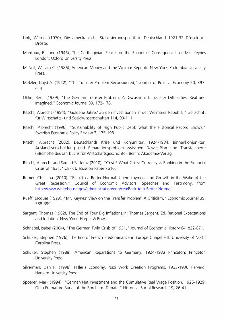
This result may be an artefact of assuming money to be endogenous when it was not. Under

looming debt constraints, inward capital mobility is reduced while outward capital mobility

temporarily increases as foreign investors rush for the exit. The basic tenets of the Mundell/Fleming

model then cannot apply, as money becomes temporarily exogenous to output. Figure 3.2 shows the

results from going against the logic of the Mundell/Fleming model and assuming money to be

exogenous to output. This ordering would reflect the prior belief that reserve flows under the Dawes

and Young Plan responded to other things than German output and may themselves be causal for

domestic adjustments.

Again, assuming money to be exogenous to output under a fixed exchange rate regime is not

innocuous. In the absence of sovereign debt limits, both the Keynesian and the monetary approach to

the transfer problem predict that cross-border capital movements ensure domestic currency is

endogenous to domestic output (see Metzler, 1942; Johnson, 1956, respectively). Conversely, if limits

to borrowing abroad exists and debt levels approach these limits, inward capital movements and

reserve flows become restricted and may cease altogether. This places an upper bound on the

circulation of a currency that is subject to international reserve requirements. As a consequence,

money becomes exogenous to output whenever the debt limit threatens to become binding.

Potentially, this could add explanatory power to the “Golden Fetters” (Eichengreen, 1992)

channel of crisis propagation under the interwar gold standard. The short-term responses of output to

a monetary shock indeed seem quite robust over time. The forecast error decompositions on the

right-hand side of Figure 3.1 suggest that slightly more than 20% of the output variation would be

explained by monetary shocks at a 6-month horizon. This is close to standard results for postwar

evidence, (see e.g. Leeper, Sims and Zha, 1996; Bernanke and Mihov, 1998; Uhlig, 2005).

15

Time variation does affect the money/income relationship at longer horizons, though. Counter

to expectation, the monetary transmission mechanism during the crisis became weaker, not stronger.

After a peak in late 1926, the long term relationship weakened already in 1927, and even further in

1929, not to recover until 1932. Only then does the impulse response function recover the hump-

shaped pattern familiar from post-war evidence, with responses reaching their maximum around two

years after the shock.

The timing of the structural breaks suggested by the time-varying parameter structure is

informative about the regime changes governing German monetary and balance of payments policies.

The 1926 spike and subsequent decline in the responses, especially at longer intervals, coincide with

the Reichsbank’s intensified efforts to sterilise capital inflows. A further break in late 1928 marks the

exit of foreign lenders from the German market, as well as the start of negotiations about the Young

Plan. The next break is visible in the last quarter of 1930, after the last tranche of the Young Plan’s

stabilization loan to Germany was disbursed. The monetary multiplier at longer intervals recovers

during 1932, surpassing its 1927 levels in the third quarter when the Young Plan was finally

abandoned.

The weakness of the responses to a monetary shock during the slump is also reflected in the

variance decompositions. Beginning in the spring of 1929, the variance explanation of output at

longer horizons starts a precipitous decline, which continues to the last quarter of 1931, after the

introduction of capital controls and Britain’s departure from the Gold Standard.

The evidence in Figure 3.2 suggests that during the contraction from 1929 to 1933, the

money-output relationship was limited to the short term impact. Further than that, the monetary

transmission mechanism appears to have lost traction: at horizons larger than four quarters, money

comes out as near-neutral. This effect is reversed in the recovery of the mid-1930s, in the

environment of a low-inflation command economy with substantial financial repression and initially

moderate money growth.

Several observations suggest themselves from the evidence gathered in these figures. First,

results are extremely sensitive to the identification procedure, suggesting a fragile and unstable

monetary transmission mechanism before 1933. Secondly, both exercises agree in assigning no active

role to the money multiplier during the downturn after 1929. Thirdly, the hiatus of the depression

separates two distinct monetary policy regimes from each other, with low effects in the 1920s and

arguably higher effects in the 1930s. These regimes are easily identifiable as the Dawes Plan, ended

by the sudden stop in the balance of payments after 1928, and the transition to credit expansion in

an autarkic economy beginning in 1933. The hiatus in between coincides with the Young Plan and its

end in mid-1932, Solving the identification problem that sets the two estimates apart is beyond the

16

scope of this chapter. But despite their vast discrepancies in results, both specifications suggest that

monetary policy during the Young Plan was not the dominant mechanism propagating the depression

in Germany.

4. Fiscal Policy: from Rules to Discretion

Stabilization after the hyperinflation of 1923 was as much a fiscal as a monetary phenomenon,

with a ban on the Reichsbank discounting treasury bills as a critical element (Sargent, 1982;

Dornbusch, 1987). Fiscal policy was kept under close surveillance during the Dawes Plan of 1924. A

reparations agent, Parker Gilbert, was installed in Berlin effect the transfer of reparations into foreign

exchange, and to report on German fiscal and monetary policy under the plan. As Germany’s currency

was shielded from reparations under transfer protection, his reports on Germany’s progress towards

increasing output, productivity, and hence her capacity to pay, were seen as critical for securing the

inflow of funds from abroad. As a consequence, the central government budget – which the agent’s

office tracked closely – went from deficits during a mild recession in 1926 to surplus in the boom of

1927/28 (Table 4.1 below). At the same time, however, lower-level government budgets as well as

the social insurance system remained in deficit.

In the aggregate, the public sector during the Dawes plan never generated the fiscal surpluses

required to pay for reparations. Table 4.1 permits a rough calculation of the fiscal sacrifice required to

transfer reparations out of surpluses. Reparations amounted to less than 2.5% of GDP, and in some

years were much lower. The cost of generating fiscal surpluses to transfer reparations would

nevertheless have been higher than that, given the prevailing public sector deficits. Simply adding

each year’s fiscal surplus (i.e., subtracting the deficit) to reparations would place the total resource

cost – including the elimination of the public deficits themselves – at 4-5% of GDP during the 1920s.

With ratios of public spending to GDP gradually approaching 30%, this would have required a change

of roughly 15% in either public spending or tax revenues even if tax elasticities were zero. (See Table

4.1.)

While such adjustments would have been substantial, they were not outside the norm: as the

data bear out, central government expenditure almost doubled between 1924 and 1929, fell by 20%

during the slump, and then grew fourfold from 1933 to 1938. The public sector share in GDP grew

from 24% in 1924 to 29% in 1929, and continued to grow from 33% in 1932 to 36% in 1936, with

a further jump to 42% in 1938

17

However, given the political constraints on raising taxes in the presence of foreign reparation

demands, the government found itself in a funding crisis as soon as the supply of foreign funds dried

out. A major loan flotation in March 1929 failed after the news on the forthcoming Young Plan had

reached the market. After that date, the government found itself essentially cut off from the credit

market and relied on the central bank instead. The price to be paid for that was a rigid deflationary

programme imposed and monitored by the bank. Except for the Young loan, which was

internationally guaranteed, carried 7% interest, and was hence well received by the market, Germany

did not place a single bond issue on the market between early 1929 and mid-1934. During this time,

the central government went through a succession of funding crises, being pushed into ever more

severe deflationary measures in order to be able to roll over its short-term debt.

Stabilization of the central government budget was to some extent due to window dressing: as

the data show, deficits persisted at lower level governments, and especially in the social security

system. However, the budget squeeze is visible here as well. Exactly the reverse tendency becomes

visible during the upswing of the 1930s: both the lower level budgets and the social security system

went into surplus, while deficit were piling up in the central government account. As a consequence

of these asymmetries, the share of public borrowing in GDP fluctuated markedly less during the 1930s

than the central government deficits would suggest.

The extent to which the onset of the fiscal crisis in early 1929 affected Germany’s borrowing

dynamics is also borne out by time series evidence. To measure the effects of fiscal policy, I specify a

time-varying VAR in output and central government deficits. To obtain the impulse response

functions, shocks to these series enter a Cholesky decomposition in the same order. This helps to

account for automatic stabilizers that affect the deficit contemporaneously with shocks to output. At

semi-annual intervals, Figure 4.1 shows the impulse response function of deficits to their own

impulse, i.e. the persistence of a deficit shock. (See Figure 4.1)

As the figure shows, the second quarter of 1929 marks a sudden regime change in fiscal policy:

the persistence of deficit shocks at longer horizons drops to nearly zero, reflecting the pressure to

swiftly restore budgetary in the face of a hardening credit constraint. Persistence recovers only during

1934, the year when military deficit spending began in earnest.

The same VAR also yields results on the dynamic multipliers of the central government’s fiscal

policy. Figure 4.2 shows the cumulative multipliers of a shock to central government budget deficits.

Identifying fiscal policy solely through the deficit implicitly assumes the multipliers of spending shocks

to be equal to those of taxation shocks. This comes at a cost, as the traditional Keynesian income-

expenditure paradigm would predict that spending multipliers exceed tax multipliers. On the other

hand, recent studies on fiscal multipliers (Bernanke and Mihov, 1998) have consistently found that

18

responses to tax shocks exceed the multipliers of spending shocks, at least at longer horizons.

Depending on the methodology applied, this discrepancy can be quite large (see also Table 4.2

below).

The principal justification for this reduced form is that it implies a temporal Cholesky ordering:

if both taxation and spending are a mixture of automatic and discretionary components, an ordering

that places deficits after output emerges quite naturally, and the discretionary component of fiscal

policy is identified without artificial assumptions about timing. (See figure 4.2)

Results for the multiplier of the discretionary component of the deficit are shown in Figure 4.2

for semi-annual intervals. As before, the dominant structural break occurs in 1934, when multipliers

and explained variance go up sharply. Before that year, the multiplier effects of deficits are miniscule,

as are the deficits themselves (see Table 4.1 above). After 1934, the variance decompositions suggest

that fiscal deficits explain between 3 and 7 % of the forecast error variance in output, which is close

to standard results from postwar evidence. Before that date, however, they indicate virtually no

explanatory power for output at all.

That the lack of deficit spending before 1933 should have had such little effect on the German

economy is not a foregone conclusion. As Table 4.1 above bears out, budget cuts during 1930-32

reduced the central government’s real expenditure by over 20%; similar figures obtain for the public

sector as a whole. Keynesian orthodoxy would predict a balanced budget cut of 4-6% of 1929 GNP

to reduce aggregate output and income by the same amount. By contrast, Figure 4.2 implies a

multiplier of hardly more than 0.1, with a maximum at 0.17 – i.e., of merely 17 pfennigs of GNP lost

per 1 reichsmark of public budget cuts.

Even these results still look pessimistic in the light of the postwar evidence gathered in Table

4.2. For a balanced budget variation, the multipliers found for U.S. data (in the wake of Blanchard

and Perotti, 2002) suggest the reverse effect: balanced budget cuts may have positive rather than

negative effects on output at longer horizons. In contrast, international evidence collected by (Ilzetzki,

Mendoza and Végh, 2010) finds that in economies operating a fixed exchange rate, fiscal shocks have

small but generally positive effects on output. Even smaller but still mostly positive multiplier effects

obtain for economies with high ratios of public debt to GDP. The results obtained in Figure 4.2 above

for Germany between 1929 and 1933 seem broadly consistent with this evidence. (See Table 4.2)

As deficits grew in 1934, so does the deficit multiplier measured in Figure 4.2. The maximum

multiplier of 0.97 is comparable to the Blanchard and Perotti (2002) estimates of deficit financed

spending shocks, but builds up far more slowly. In this it is comparable to the temporal profile found

by Mountford and Uhlig (2009) although it comes out somewhat higher. In Table 4.2 we also note

19

the nearly perfect fit with the multipliers for closed economies found by Ilzetzky, Mendoza and Veigh

(2011). Clearly, the effects of deficit spending in the German upswing after 1933 are very much in

line with the postwar experience.

The effects of fiscal tightening have been the subject matter of intense debate also for the

Great Recession after 2008. While a consensus on positive short term effects of fiscal stimuli seems to

have emerged (see Corsetti, Meier and Mueller, 2009; Cwik and Wieland, 2010; Coenen, Straub and

Trabandt, 2011), there is evidence casting doubt on the conclusion that by symmetry, austerity in the

presence of high debt levels has contractionary effects (Alesina and Ardagna, 2010; Cochrane, 2011;

Corsetti et al., 2011). Earlier research on episodes of fiscal austerity found mixed evidence but

emphasized the possibility of favourable outcomes (see Alesina and Drazen, 1991; Bertola and

Drazen, 1991).

By comparison, the evidence in Figure 4.2 points to an intermediate case: fiscal multipliers for

during the contraction period of 1929 to 1932 are small but still positive, indicating that austerity did

contract economic activity, although probably not by as much as has commonly been taken for

granted in the historical literature.

Drawing the results of this section together, the evidence shows how fiscal austerity during the

slump after 1929 changed the time series characteristics. Fiscal shocks lost their persistence in mid-

1929 when the first funding crisis occurred, and regained it when deficit spending began in 1934.

Fiscal multipliers during the recession remained small overall. Multipliers increased again with the

transition to exchange rate control and managed credit expansion. For both regimes, the multiplier

estimates are in line with post-war evidence. Overall, these results assign a minor role to fiscal policy

during the slump, but also suggest only a limited contribution to recovery after 1933.

5. The Wage Channel of Crisis Propagation

As a consequence of revolution in 1918, the German economy arrived to the reconstructed

Gold Standard with a highly interventionist labour market regime. This included the eight-hour day,

workplace councils, collective bargaining and mandatory state arbitration of labour disputes. Wage

determination soon was a matter of party coalition politics, and arbitration by government officials

became the rule (Feldman, 1993). Until 1929, wages increased substantially, and wage compression

favoured unskilled workers (Bry, 1960). Still, output and to a lesser extent employment increased as

well, as the economy continued to recover from the hyperinflation of the early 1920s. (See Table 5.1e)

20

As the data in Table 5.1 bear out, wages outstripped productivity growth during the late

1920s, leading to a substantial rise in unit labour cost. In spite of the drastic fall in output and

employment during the subsequent slump, both real wages and productivity continued to grow.

Again, however, wages increased faster. Only after 1934 was this tendency reversed, and unit labour

cost gradually declined to the levels of the mid-1920s.

To identify regime changes that may have influenced the labour demand schedule, we employ

the same time varying VAR technique as before. In a setup that controls for output and ex-post real

interest rates, the responses of labour demand to real wage shocks again reveal a regime-dependent

pattern2. (See figure 5.1)

At a 6-month horizon, the wage elasticity of labour demand remains more or less stable at

values around -1, which conforms to theoretical priors and to earlier results for interwar Germany and

Britain (Broadberry and Ritschl, 1995). At longer lags, the effects are again strongly regime

dependent. From 1927 into early 1930, the labour demand schedule at longer horizons almost

appears to break down. During the downturn, it recovers dramatically, suggesting strong and

persistent effects of real wage shocks on labour demand. The schedule goes back to standard

parameter values and loses its volatility during the recovery of the mid-1930s. A look at the variance

decomposition suggests high explanatory power for wage shocks throughout; wage shocks during

1931/2 explain up to 65% of the forecast error variance in output. This is gradually reduced as

recovery sets in.

These results suggest that real wage rigidity – or more precisely, the continuing rise of unit

wage cost in excess of productivity growth – was a major channel crisis propagation, consistent with

findings of Borchardt (1990). Keeping real wages high through political arbitration had strong,

pernicious effects on employment after 1929.

Prior to the depression, however, wages apparently did not affect employment very much. This

anomaly coincides with the period of heavy capital inflows – of commercial credit until 1928 and of

stabilization loans further until 1930 – into the German economy. These inflows temporarily alleviated

the wage pressure emanating from collective wage bargaining and arbitration. This would be

consistent with findings that attribute little effect to wage pressure during the late 1920s (see e.g.

Voth, 1995). As soon as the music stopped, however, adjustment set in rapidly, with detrimental

consequences for employment.

2 The variables included are (in this order of exogeneity in the Cholesky decomposition) quarterly GDP, com-

mercial paper rates, non-agricultural total hours and real wages per person employed. All data from Ritschl

(2002, Appendix C.2).

21

Similar patterns become visible in the responses of investment activity to wages. Controlling for

output and the cost of capital, the dynamic relationship between investment and wages until 1929

appears to be weak and ambiguous, with responses changing signs at longer horizons. After that,

however, investment responded strongly and negatively to wage shocks at longer horizons. This effect

persists until 1933 and only gradually weakens as recovery gets underway. (See Figure 5.2)

Figure 5.2 shows the wage elasticity of the demand for capital goods, measured by orders of

factory equipment (data from VDMA, 1927; 1930). According to these results, wages seem to have

little explanatory power for investment in the late 1920s (see on this Ritschl, 1994; Spoerer, 1994;

Voth, 1994). However, this changes abruptly in early 1929; during the depression over 50% of

investment activity is explained by wage shocks at longer lags. This suggests a second wage channel

of propagation of the depression in Germany, which goes beyond the labour market itself (consistent

with a claim by Borchardt, 1980).

Drawing the results of this section together, wages come out as the predominant channel of

crisis propagation in Germany during the depression. Wages appear to have affected economy activity

in two ways: directly, going through the labour market, and indirectly, by their effects on the decision

to invest. The wage channel provides what we could not find for monetary and even fiscal policy

during the slump: a quantitatively important transmission mechanism that translated the sudden stop

in the German current account after 1928 into a decline in output and employment.

6. Conclusions and Implications for Today

Fiscal austerity programmes have a reputation for facing a Keynesian Laffer curve and thus be

self-defeating. Potential dangers and pitfalls of this policy have been highlighted prominently during

the Great Recession after 2008 (prominently by Krugman, 2008, in a fiery criticism of German plans

to balance the budget after 2008). Germany’s fiscal policy during the Great Depression of the 1930s

was just such a policy: it was strictly deflationary, aimed to balance the budget, and followed many of

the precepts implicit in the later Washington Consensus. Applied during a slump of catastrophic

proportions, Germany’s strategy of deflation has drawn the ire of commentators at all times.

This chapter has placed this policy in the context of Germany’s mounting foreign debt crisis

during 1929-1931. German fiscal policy adhered to orthodox recipes, not so much out of misguided

ideology but in an attempt to avoid defaulting on reparations. Transition from the earlier Dawes plan

with its lax payment conditions to the much stricter Young Plan had marked a sudden regime change

in fiscal policy. From mid-1929 to late 1933, balancing the budget was the paramount fiscal priority.

22

Success of this policy was mixed. Whilst it reached the limited goal of averting outright default on

reparations, it ultimately failed in its attempt to keep current on Germany’s commercial foreign debt.

There is general agreement that this course of action contributed to political radicalisation. Political

pressure to pay by creditors abroad and to default by voters at home put the government in the

precarious position of an agent with two principals having diametrically opposed interests. The effects

on the legitimacy of the Weimar Republic in the eyes of the population were detrimental.

This chapter has argued that the 1929 fiscal reversal in Germany came as a consequence of a

sudden stop in the current account, following a pattern that closely resembles post-war sovereign

debt crises. Cut off from foreign credit markets, the German government resorted to seeking a

political stabilization loan as well as assistance from the central bank. Both came with a long laundry

list of conditions, ranging from budget and wage cuts to reductions in administered prices; essentially

the same conditionality that has been attached to recent relief programmes in Southern Europe.

Germany’s deflationary policy is thus an early case of an international stabilization programme having

run into trouble.

The quantitative evidence presented in this paper suggests that, nevertheless, neither fiscal nor

monetary policy were the principal mechanism of crisis propagation in Germany. Fiscal multipliers

during the austerity phase were positive but low, which would be consistent with post-war evidence

on balanced budget variations. The dominant channel of crisis transmission and propagation we

found is real wage rigidity: though nominal wages did fall, producer prices declined faster, with direct

effects on labour demand and indirect effects on investment. This highlights a fundamental dilemma

of German deflationary policy, the inability to enforce wage cuts that would outpace price declines

and thus result in real wage decline. As a consequence, real wages in Germany rose during the

depression, as did unit labour cost.

The political economy of this phenomenon is not difficult to understand, and it gives reasons

for concern. There is general agreement that unemployment after 1929 caused the rise of Nazi and

communist votes and thus brought about the political collapse of the Weimar Republic. However, the

mechanism linking the two does not appear to be as straightforward as early research (Frey and

Weck, 1981; critiqued by Falter, 1986) would have it. Recent research suggests a potential for right

wing extremism that had deep historical and cultural roots, although this would not itself explain the

rise of the extremist vote since 1930 (Voigtlaender and Voth, 2012). Indeed, the increase in the Nazi

vote came predominantly from the lower middle class worried about being thrown into

unemployment and deprivation (King et al., 2008).

Similar destabilising mechanisms might be threatening countries with weak institutions today.

Governments confronted with a voter base susceptible to radicalisation would find it politically

23

expedient to eschew radical austerity measures. In a two-party system and its derivatives, participants

might then play a waiting game, with each side attempting to place the onus on the other in a quick

succession of unstable governments, thus postponing stabilization (Alesina and Drazen, 1991).

Germany’s case is also instructive about the option of currency devaluation. Given that her debt

was gold denominated, Germany opted for capital controls instead of open devaluation, a decision

largely due to creditor pressure: U.S. negotiators signalled to the Germans during 1931 that imposing

capital controls would be more acceptable than open devaluation and default on the gold clauses in

the loan contracts (Ritschl, 2002). Last, the German crisis provides lessons about the international

repercussions of a large economy defaulting, including transatlantic feedbacks on the U.S. economy

(Ritschl and Sarferaz, 2010), the breakup of fixed exchange rate arrangements (Accominotti 2011)

and the increase of protectionism.

In the light of these lessons, it is instructive to pursue the parallels between Germany’s debt

crisis in 1931 and the Southern European debt crisis since 2009/10 a bit further. The first parallel is

that the debtor country would adopt internal, fiscal devaluation instead of an open breakaway from

the common monetary standard. This is all the more striking as the interwar gold standard was not a

currency union: both the national currencies and the respective national payment systems continued

to exist, enabling the member countries to exit at low transaction cost. The second parallel is the

internal devaluation itself: Germany’s policy of deflation between 1929 and 1932 is the quintessential

economic history textbook example of a pre-Keynesian policy response to a recession, when in fact it

was a policy of austerity in the face of a looming sovereign debt crisis. The third parallel is a

government of technocrats with only weak public support, installed to carry out austerity policies at

the behest of the foreign creditor countries. In Germany, this arrangement eroded the support for

democratic parties among voters and hastened social unrest, mass protests, and politically motivated

violence – in 1932 alone, authorities counted 2000 deaths in such incidents (Thamer, 1986). Violent

mass protest against austerity measures in southern Europe has not been the norm but recent

incidents suggest a potential for radicalization and societal disintegration. The fourth parallel is the

failure of real wages to fall during the austerity period. In spite of emerging mass unemployment, real

wages and unit labour costs continued to increase in Germany during 1929-32, a phenomenon that

has been observed in the Mediterranean basin during the recent crisis as well (see e.g. EEAG, 2012) .

The last – potential – parallel is the breakup of the currency system by contagion. Germany itself,

pressed but also incentivised by its creditors, responded to its own financial meltdown by financial

repression and capital controls instead of devaluation. However, the knock-on effects of Germany’s

financial crisis on Britain’s banking system seem to have been instrumental in Britain’s departure from

Gold (Accominotti, 2011).

24

We do not have the counterfactual of what would happened had different policies toward the

German crisis been pursued. Finding a feasible counterfactual was perhaps the biggest and most

contentious issue of Weimar historiography in the 1980s and 1990s. The essence of the criticism was

that Germany should have devalued openly and at an early stage, thus avoiding excessive fiscal

contraction (Holtfrerich, 1982; Ferguson and Temin, 2003), while others have pointed out that given

Germany’s recent hyperinflation (Borchardt, 1979; 1984), the actions of her foreign creditors (Ritschl,

2002), and the weakness of her national banking system (Schnabel, 2004), devaluation was not an

easy game to play. Very similar counterfactuals have been popular in the current crisis of the

European periphery. While it is too early to tell whether the analogy with interwar Germany will carry

through, the indication again seems to be that creditor pressure, not lacking economic insight is what

might keep the debtor countries of Southern Europe within the Eurozone.

References

Alesina, Alberto (2011), "Fiscal Policy after the Great Recession," Barcelona GSE Lecture XXI.

Alesina, Alberto and Silvia Ardagna (2010), Large Changes in Fiscal Policy: Taxes versus Spending,in: Jeffrey Brown, Ed. Tax Policy and the Economy, Volume 24, Chicago: Chicago University Press.

Alesina, Alberto and Allen Drazen (1991), "Why Are Stabilizations Delayed?," American Economic Review 81, 1170-1188.

Bernanke, Ben and L. Mihov (1998), "Measuring Monetary Policy," Quarterly Journal of Economics 113, 869-902.

Bertola, Giuseppe and Allen Drazen (1991), "Trigger Points and Budget Cuts: Explaining the Effects of Fiscal Austerity," American Economic Review 83, 11-26.

Blanchard, Olivier and Roberto Perotti (2002), "An Empirical Characterization of the Dynamic Effects of Changes in Government Spending and Taxes on Output," Quarterly Journal of Economics 117, 1329-1368.

Borchardt, Knut (1979), "Zwangslagen und Handlungsspielräume in der großen Wirtschaftskrise der frühen dreißiger Jahre," Jahrbuch der Bayerischen Akademie der Wissenschaften85-132.

Borchardt, Knut (1980), Wirtschaftliche Ursachen des Scheiterns der Weimarer Republik,in: K.-D. Erdmann and H. Schulze, Eds., Weimar, Selbstpreisgabe einer Demokratie: Eine Bilanz heute, Düsseldorf: Droste, 211-249.

Borchardt, Knut (1984), "Could and Should Germany Have Followed Britain in Leaving the Gold Standard?," Journal of European Economic History 13, 471-498.

Borchardt, Knut (1990), A Decade of Debate About Bruening's Economic Policy,in: J. v. Kruedener, Ed. Economic Crisis and Political Collapse. The Weimar Republic 1924-1933, Oxford: Berg, 99-151.

25

Broadberry, Stephen and Albrecht Ritschl (1995), "Real Wages, Productivity, and Unemployment in Britain and Germany during the 1920s," Explorations in Economic History 32, 327-349.

Bry, Gerhard (1960), Wages in Germany, 1871-1945 Princeton: Princeton University Press.

Cochrane, John (2011), "Understanding Policy in the Great Recession: Some Unpleasant Fiscal Arithmetic," European Economic Review 55, 2-30.

Coenen, Guenther, Roland Straub and Mathias Trabandt (2011), "Fiscal Policy and the Great Recession in the Euro Area," mimeo, European Central Bank.

Corsetti, Giancarlo, et al. (2011), "Sovereign Risk and the Effects of Fiscal Retrenchment in Deep Recessions," American Economic Review 101.

Corsetti, Giancarlo, A Meier and G Mueller (2009), "Fiscal Stimulus with Spending Reversals," IMF Working Paper 09/106.

Cwik, T and Volker Wieland (2010), "Government Spending Multipliers and Spillovers in the Euro Area," ECB Working Paper 1276.

Dornbusch, Rüdiger (1987), Lessons from the German Inflation Experience of the 1920s,in: R. Dornbusch et al., Ed. Macroeconomics and Finance: Essays in Honor of Franco Modigliani, Cambridge: Cambridge University Press, 337-366.

Eaton, Jonathan, M Gersovitz and Joseph Stiglitz (1986), "The Pure Theory of Country Risk," European Economic Review 30, 481-513.

EEAG (2012), The EEAG Report on the European Ecoomy 2012 Munich: CESifo.

Eichengreen, Barry (1992), Golden Fetters. The Gold Standard and the Great Depression 1919-1939 Oxford: Oxford University Press.

Eichengreen, Barry and Ricardo Hausman (1999), Exchange Rates and Financial Fragility,in: Federal Reserve Bank of Kansas, Ed. New Challenges for Monetary Policy, 329-368.

Falter, W., et al. (1986), Wahlen und Abstimmungen in der Weimarer Republik. Materialien zum Wahlverhalten 1919-1932 München: Beck.

Feinstein, Charles, Peter Temin and Gianni Toniolo (1997), The European Economy Between the Wars Oxford: Oxford University Press.

Feldman, Gerald (1993), The Great Disorder. Politics, Economics, and Society in the German Inflation, 1914-1924 Oxford: Oxford University Press.

Ferguson, Thomas and Peter Temin (2003), "Made in Germany: the Currency Crisis of 1931," Research in Economic History 31, 1-53.

Frey, Bruno and Hannelore Weck (1981), "Hat Arbeitslosigkeit den Aufstieg des Nationalsozialismus bewirkt?," Jahrbücher für Nationalökonomie und Statistik 196, 1-31.

Gilbert, Parker (1925-30), Report of the Agent General for Reparation Payments Berlin: Agent General.

26

Hamilton, James D. (1994), Time Series Analysis Princeton: Princeton University Press.

Hardach, Karl (1980), The Political Economy of Germany in the 20th Century Berkeley: University of California Press.

Helbich, W. (1962), Die Reparationen in der Ära Brüning: Zur Bedeutung des Young-Plans für die deutsche Politik 1930 bis 1932 Berlin: Colloquium-Verlag.

Holtfrerich, Carl-Ludwig (1982), "Alternativen zu Brünings Politik in der Weltwirtschaftskrise?," Historische Zeitschrift 235, 605-631.

Holtfrerich, Carl-Ludwig (1986), The German Inflation New York: de Gruyter.

Holtfrerich, Carl-Ludwig (1990), Was the Policy of Deflation in Germany Unavoidable?,in: Juergen v. Kruedener, Ed. Economic Crisis and Political Collapse. The Weimar Republic 1924-1933, Oxford: Berg, 63-80.

Ilzetzki, Ethan, Enrique Mendoza and Carlos Végh (2010), "How Big (Small?) are Fiscal Multipliers?," NBER Working Paper 16479.

James, Harold (1985), The Reichsbank and Public Finance in Germany, 1924-1933: A Study of the Politics of Economics during the Great Depression Frankfurt am Main: Knapp.

James, Harold (1986), The German Slump: Politics and Economics, 1924-1936 Oxford: Clarendon Press.

Johnson, Harry G. (1956), "The Transfer Problem and Exchange Stability," Journal of Political Economy 64, 212-225.

Keynes, John Maynard (1920), The Economic Consequences of the Peace London: Macmillan.

Keynes, John Maynard (1922), A Revision of the Treaty London: Macmillan.

Keynes, John Maynard (1926), Germany's Coming Problem,in: C. Johnson, Ed. The Collected Writings of John Maynard Keynes Vol. XVIII: Activities 1922-1932. The End of Reparations, London: Macmillan (1978), 271-277.

Keynes, John Maynard (1929), "The German Transfer Problem," Economic Journal 39, 1-7.

King, G. , et al. (2008), "Ordinary Economic Voting Behavior in the. Extraordinary Election of Adolf Hitler," Journal of Economic History 68, 951-996.

Klug, Adam (1993), The German Buybacks 1932-1939: A Cure for Overhang? (=Princeton Studies in International Finance), Princeton: Princeton University Press.

Krugman, Paul (2008), "The Economic Consequences of Herr Steinbrueck," New York Times December 11, 2008.

Leeper, Eric, Christopher Sims and Tao Zha (1996), "What Does Monetary Policy Do?," Brookings Papers on Economic Activity Series 2, 1-63.

27

Link, Werner (1970), Die amerikanische Stabilisierungspolitik in Deutschland 1921-32 Düsseldorf: Droste.

Mantoux, Etienne (1946), The Carthaginian Peace, or the Economic Consequences of Mr. Keynes London: Oxford University Press.

McNeil, William C. (1986), American Money and the Weimar Republic New York: Columbia University Press.

Metzler, Lloyd A. (1942), "The Transfer Problem Reconsidered," Journal of Political Economy 50, 397-414.

Ohlin, Bertil (1929), "The German Transfer Problem: A Discussion, I: Transfer Difficulties, Real and Imagined," Economic Journal 39, 172-178.

Ritschl, Albrecht (1994), "Goldene Jahre? Zu den Investitionen in der Weimarer Republik," Zeitschrift für Wirtschafts- und Sozialwissenschaften 114, 99-111.

Ritschl, Albrecht (1996), "Sustainability of High Public Debt: what the Historical Record Shows," Swedish Economic Policy Review 3, 175-198.

Ritschl, Albrecht (2002), Deutschlands Krise und Konjunktur, 1924-1934. Binnenkonjunktur, Auslandsverschuldung und Reparationsproblem zwischen Dawes-Plan und Transfersperre (=Beihefte des Jahrbuchs für Wirtschaftsgeschichte), Berlin: Akademie-Verlag.

Ritschl, Albrecht and Samad Sarferaz (2010), "Crisis? What Crisis: Currency vs Banking in the Financial Crisis of 1931," CEPR Discussion Paper 7610.

Romer, Christina. (2010). "Back to a Better Normal: Unemployment and Growth in the Wake of the Great Recession." Council of Economic Advisors: Speeches and Testimony, from http://www.whitehouse.gov/administration/eop/cea/Back-to-a-Better-Normal.

Rueff, Jacques (1929), "Mr. Keynes' View on the Transfer Problem: A Criticism," Economic Journal 39, 388-399.

Sargent, Thomas (1982), The End of Four Big Inflations,in: Thomas Sargent, Ed. Rational Expectations and Inflation, New York: Harper & Row.

Schnabel, Isabel (2004), "The German Twin Crisis of 1931," Journal of Economic History 64, 822-871.

Schuker, Stephen (1976), The End of French Predominance in Europe Chapel Hill: University of North Carolina Press.

Schuker, Stephen (1988), American Reparations to Germany, 1924-1933 Princeton: Princeton University Press.

Silverman, Dan P. (1998), Hitler's Economy. Nazi Work Creation Programs, 1933-1936 Harvard: Harvard University Press.

Spoerer, Mark (1994), "German Net Investment and the Cumulative Real Wage Position, 1925-1929: On a Premature Burial of the Borchardt Debate," Historical Social Research 19, 26-41.

28

Thamer, Hans-Ulrich (1986), Verführung und Gewalt: Deutschland 1933-1945 (=Die Deutschen und ihre Nation), Berlin: Siedler.

Toniolo, Gianni (2005), Central Bank Cooperation at the Bank of International Settlements, 1930-1973, Cambridge: Cambridge University Press.

Uhlig, Harald (2005), "What are the Effects of Monetary Policy on Output?," Journal of Monetary Economics 52, 381-419.

VDMA (1927), Statistisches Handbuch für die deutsche Maschinenindustrie 1927 Berlin: VDMA.

VDMA (1930), Statistisches Handbuch für die deutsche Maschinenindustrie 1930 Berlin: VDMA.

Voigtlaender, Nico and Hans-Joachim Voth (2012), "Persecution Perpetuated: The Medieval Origins of Anti-Semitic Violence in Nazi Germany," Quarterly Journal of Economics (forthcoming).

Voth, Hans-Joachim (1994), "Much Ado about Nothing? A Note on Investment and Wage Pressure in Weimar Germany, 1925-1929," Historical Social Research 19, 124-139.

Voth, Hans-Joachim (1995), "Did High Wages or High Interest Rates Bring down the Weimar Republic?," Journal of Economic History 55, 801-821.

29

Figure 3.1: The dynamic multiplier effects of money demand shocks on output in a time-varying VAR

Output and prices assumed exogenous to money

-0.8

-0.6

-0.4

-0.2

0.0

0.2

0.4

0.6

1925

:01

1926

:01

1927

:01

1928

:01

1929

:01

1930

:01

1931

:01

1932

:01

1933

:01

1934

:01

1935

:01

1936

:01

1937

:01

1938

:01

TVAR impulse response functions after 2,4,6, and 8 quarters

IRFYM_2 IRFYM_4

IRFYM_6 IRFYM_8

02468

10121416

1925

:01

1926

:01

1927

:01

1928

:01

1929

:01

1930

:01

1931

:01

1932

:01

1933

:01

1934

:01

1935

:01

1936

:01

1937

:01

1938

:01

% d

er P

rogn

osef

ehle

rvar

ianz

Contribution to TVAR variance decomposition after 2,4,6, and 8 quarters

VARDYM_2 VARDYM_4

VARDYM_6 VARDYM_8

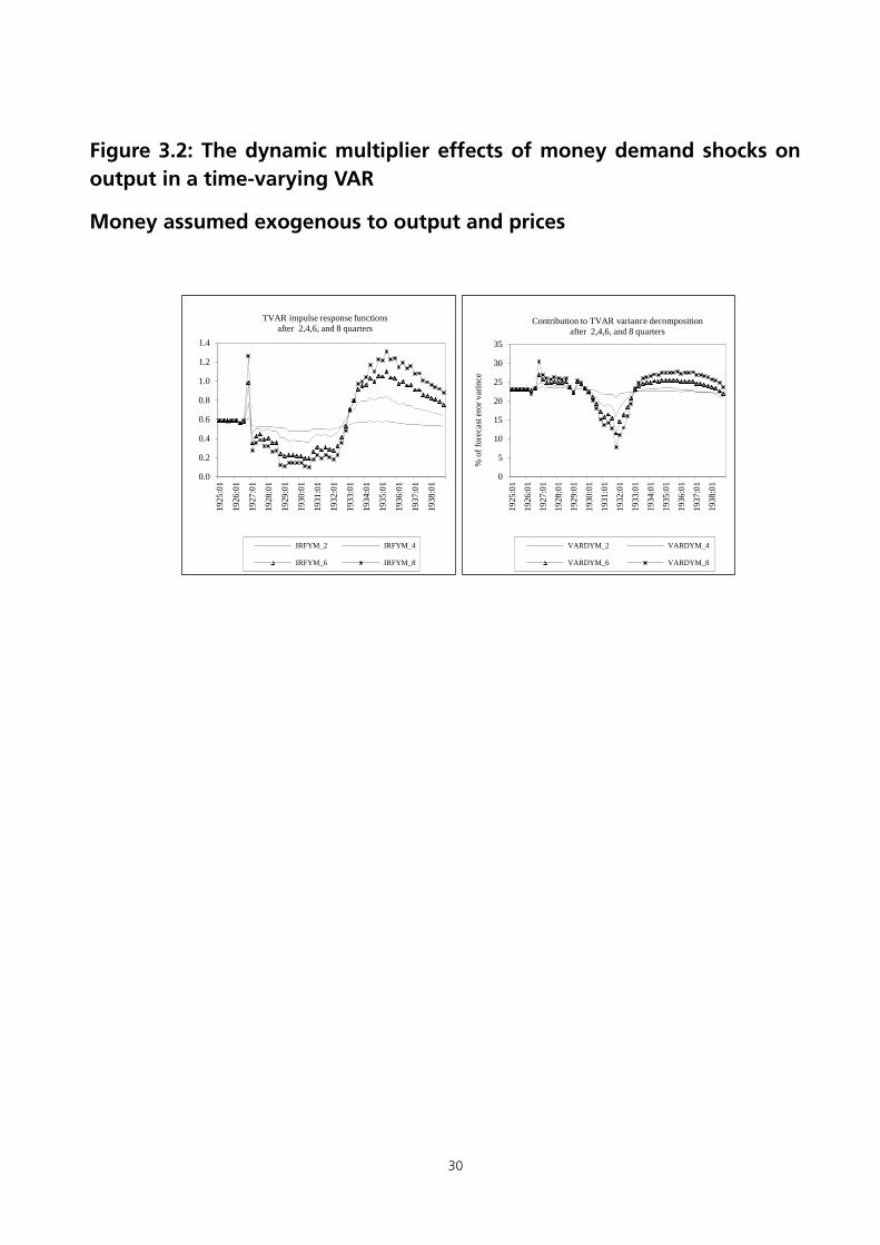
30

Figure 3.2: The dynamic multiplier effects of money demand shocks on output in a time-varying VAR

Money assumed exogenous to output and prices

0.0

0.2

0.4

0.6

0.8

1.0

1.2

1.4

1925

:01

1926

:01

1927

:01

1928

:01

1929

:01

1930

:01

1931

:01

1932

:01

1933

:01

1934

:01

1935

:01

1936

:01

1937

:01

1938

:01

TVAR impulse response functions after 2,4,6, and 8 quarters

IRFYM_2 IRFYM_4

IRFYM_6 IRFYM_8

0

5

10

15

20

25

30

35

1925

:01

1926

:01

1927

:01

1928

:01

1929

:01

1930

:01

1931

:01

1932

:01

1933

:01

1934

:01

1935

:01

1936

:01

1937

:01

1938

:01

% o

f for

ecas

t ero

r var

ince

Contribution to TVAR variance decomposition after 2,4,6, and 8 quarters

VARDYM_2 VARDYM_4

VARDYM_6 VARDYM_8

31

Figure 4.1: The persistence of central government budget deficit shocks in a time-varying VAR

-0.1

0.0

0.1

0.2

0.3

0.4

0.5

0.6

0.7

0.8

0.9

1925

:01

1926

:01

1927

:01

1928

:01

1929

:01

1930

:01

1931

:01

1932

:01

1933

:01

1934

:01

1935

:01

1936

:01

1937

:01

1938

:01

TVAR impulse response functions after 2, 4, 6, and 8 quarters

IRFDD_2 IRFDD_4 IRFDD_6 IRFDD_8

32

Figure 4.2: The dynamic multiplier effects of central government budget deficits shocks on output in a time-varying VAR

-0.2

0.0

0.2

0.4

0.6

0.8

1.0

1.2

1.4

1925

:01

1926

:01

1927

:01

1928

:01

1929

:01

1930

:01

1931

:01

1932

:01

1933

:01

1934

:01

1935

:01

1936

:01

1937

:01

1938

:01

Cumulative fiscal multipliers from TVAR impulse response functions

after 2,4,6, and 8 quarters

IRFYD_2 IRFYD_4

IRFYD_6 IRFYD_8

0

1

2

3

4

5

6

7

8

1925

:01

1926

:01

1927

:01

1928

:01

1929

:01

1930

:01

1931

:01

1932

:01

1933

:01

1934

:01

1935

:01

1936

:01

1937

:01

1938

:01

% o

f for

ecas

t err

or v

aria

nce

Contribution to TVAR variance decompositions after 2,4,6, und 8 quarters

VARDYD_2 VARDYD_4

VARDYD_6 VARDYD_8

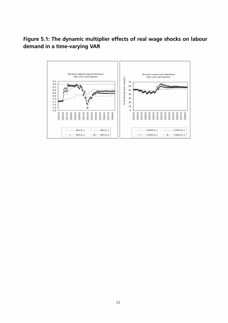
33

Figure 5.1: The dynamic multiplier effects of real wage shocks on labour demand in a time-varying VAR

-1.8-1.6-1.4-1.2-1.0-0.8-0.6-0.4-0.20.00.2

1925

:01

1926

:01

1927

:01

1928

:01

1929

:01

1930

:01

1931

:01

1932

:01

1933

:01

1934

:01

1935

:01

1936

:01

1937

:01

1938

:01

Recursive impulse response fucntions after 2,4,6, and 8 quarters

IRFLW_2 IRFLW_4

IRFLW_6 IRFLW_8

010203040506070

1925

:01

1926

:01

1927

:01

1928

:01

1929

:01

1930

:01

1931

:01

1932

:01

1933

:01

1934

:01

1935

:01

1936

:01

1937

:01

1938

:01

% o

f for

ecas

t err

or v

aria

nce

Recursive variance decompositions after 2,4,6, and 8 quarters

VARDLW_2 VARDLW_4

VARDLW_6 VARDLW_8

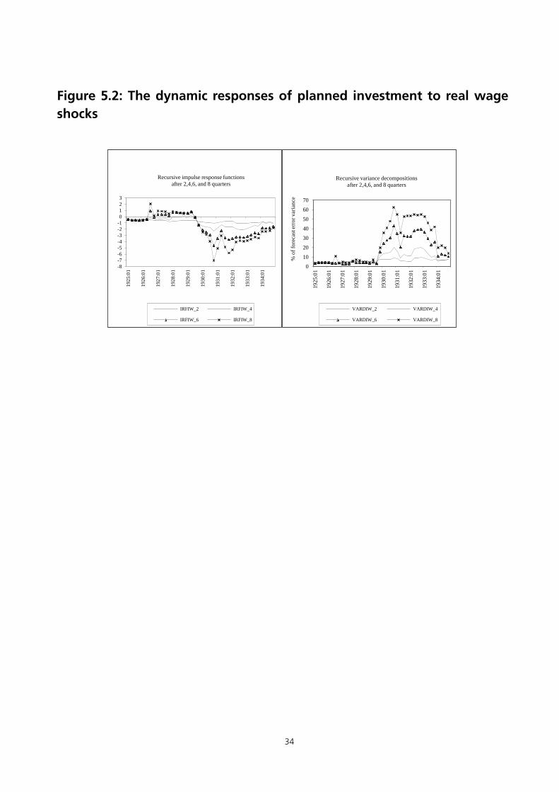
34

Figure 5.2: The dynamic responses of planned investment to real wage shocks

-8-7-6-5-4-3-2-10123

1925

:01

1926

:01

1927

:01

1928

:01

1929

:01

1930

:01

1931

:01

1932

:01

1933

:01

1934

:01

Recursive impulse response functions after 2,4,6, and 8 quarters

IRFIW_2 IRFIW_4

IRFIW_6 IRFIW_8

0

10

20

30

40

50

60

70

1925

:01

1926

:01

1927

:01

1928

:01

1929

:01

1930

:01

1931

:01

1932

:01

1933

:01

1934

:01

% o

f for

ecas

t err

or v

aria

nce

Recursive variance decompositions after 2,4,6, and 8 quarters

VARDIW_2 VARDIW_4

VARDIW_6 VARDIW_8

35

Table 2.1: Reparations and German GNP

1913

1925

1929

1931

Nominal GNP (bn reichs-marks)

51

71.1

88.4

68.0

Reparations (bn gold marks / reichsmarks)

--- as percentage of nominal GNP ---

(a) London ultima-tum

A bonds (net in-demnity)

12

23.5

16.9

13.6

A + B bonds (38 bn, for inter-allied war debt) 50

98.0

70.3

56.5

A + B + C bonds (82 bn)

132

258.8

185.5

149.2

(b) Dawes Plan of 1924

46

59.0

47.5

(c) Young Plan of 1929/30 37

41.8

54.4

Source: Hardach (1980), Holtfrerich (1990), Ferguson (1998), Ritschl (1996, 2002)

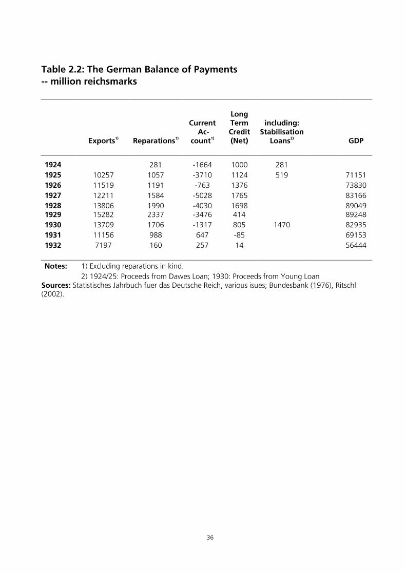
36

Table 2.2: The German Balance of Payments -- million reichsmarks

Exports1) Reparations1)

Current Ac-

count1)

Long Term Credit (Net)

including: Stabilisation

Loans2)

GDP

1924

281 -1664 1000 281

1925 10257 1057 -3710 1124 519

71151

1926 11519 1191 -763 1376

73830 1927 12211 1584 -5028 1765

83166

1928 13806 1990 -4030 1698

89049 1929 15282 2337 -3476 414

89248

1930 13709 1706 -1317 805 1470

82935 1931 11156 988 647 -85

69153

1932 7197 160 257 14

56444

Notes: 1) Excluding reparations in kind.

2) 1924/25: Proceeds from Dawes Loan; 1930: Proceeds from Young Loan

Sources: Statistisches Jahrbuch fuer das Deutsche Reich, various isues; Bundesbank (1976), Ritschl (2002).

37

Table 2.3: Foreign Debts and GDP -- million reichsmarks --

Commercial Reparations GDP

Foreign Debt/GDP

(%)

1928 27 40 89.0 75.2 1929 31 46/37 89.2 86.3/76.2 1930 32.6 35 82.9 81.5 1931 (mid-year) 33.6 34 68.5 98.7 1931 (end) 26.6 34 58.1 104.3 1932 25.9 -- 56.4 45.9

Notes: Sources:

Figures in italics are quarterly, annualized. Reparations 1929: Dawes Plan / Young Plan (NPV) Bundesbank (1976), Ritschl (2002).

38

Table 4.1: Key indicators of public expenditure (thousand mill. reichsmarks, current values)

Gov't Expenditure and Transfers

of which: Surplus/Deficit

Cen-tral

gov't Public sector

Repara-tions

Central gov't

Public sec-tor GDP CPI1)

1924

0.77 1925 5.38 16.92 1.08 -0.29 -0.52 71.15 141.9

1926 6.12 19.13 1.30 -0.78 -1.91 73.83 142.2 1927 6.55 21.93 1.71 0.01 -0.93 83.17 147.9 1928 6.87 23.77 2.16 0.15 -0.64 89.05 151.7 1929 7.75 26.05 1.96 -0.77 -2.23 89.25 154.0 1930 7.93 26.27 1.88 -0.16 -2.36 82.93 148.1 1931 6.52 22.71 0.99 0.36 -1.07 69.15 136.1 1932 5.75 18.91 0.18 0.13 -0.60 56.44 120.6 1933 6.49 19.84 0.15 -0.80 -0.78 57.72 118.0 1934 9.62 23.13 0.05 -3.41 -2.82 64.38 121.1 1935 11.85 25.08

-4.37 -3.22 71.75 123.0

1936 13.25 26.36

-3.52 -1.67 79.65 124.5 1937 18.62 32.06

-6.04 -3.61 89.11 125.1

1938 26.05 41.29

-9.46 -7.78 99.19 125.6 Notes: 1) 1913 = 100. Sources: Statistisches Jahrbuch fuer das Deutsche Reich, various issues.

German Federal Archive, Economics Ministry Collections, R7.

39

Table 4.2: Multiplier effects of a public spending increase Results for Germany 1934-38 vs estimates and calibrations for post-war data I. Deficit-financed spending shock

1 quarter 4 quarters 8 quarters

Germany 1934-38 Postwar data

0.14*) 0.42 0.97

Blanchard/Perotti (2002) 0.9 0.55 0.65 (Simulation) antici-pated

1.8 1.7 1.7 to 2.2

(Simulation) unantici-pated

1.2 0.8 0.9

Mountford/Uhlig (2006) 0.44 0.42 0.67 Leeper et al. (2011) NK autarky, G non-traded

1.18

0.91

0.64**)

Ilzetzky/Mendoza/Veigh (2011) Closed economy

0.11

0.6

0.9

II. Balanced-budget spend-ing shock

1 quarter

4 quarters

8 quarters

Germany 1929-33 Postwar data

0.04*) 0.10 0.12

Blanchard/Perotti (2002) 0.2 -0.52 -0.67 (Simulation) antici-pated

1 to 1.5 0.3 to 1 0.1 to 1.1

(Simulation) unantici-pated

0.6 -0.1 0.4

Mountford/Uhlig (2006) 0.25 -0.79 -2.55 Ilzetzky/Mendoza/Veigh (2011) Fixed exchange rate High-debt/income ra-tio

0.04 0.06

0.25 0.06

0.5

-0.75

*) 2 quarters **) 10 quarters

40

Table 5.1: Real Wages and Productivity (1925 = 100)

Wages Output Employment Unemployment Productivity

Unit Labour Cost

- per cent -

1925 100.0 100.0 100.0 4.0 100.0 100.0

1926 118.5 101.4 92.8 11.8 109.3 108.5 1927 121.3 111.8 101.0 7.1 110.7 109.6 1928 119.2 115.4 105.5 7.7 109.4 109.0 1929 127.0 113.6 103.4 10.4 109.9 115.6 1930 132.0 106.0 96.4 17.2 110.0 120.0 1931 142.2 93.8 83.5 25.5 112.3 126.5 1932 144.5 84.9 73.2 31.5 116.0 124.6 1933 149.7 91.2 75.3 27.2 121.1 123.7 1934 143.9 100.9 85.8 15.7 117.5 122.5 1935 140.9 113.2 92.2 12.1 122.8 114.8 1936 138.4 125.9 100.1 9.6 125.8 110.0 1937 135.4 140.0 107.8 5.0 129.8 104.2 1938 133.4 153.4 114.9 2.2 133.5 99.9

Source: Statistisches Jahrbuch fuer das Deutsche Reich, various issues; Ritschl (2002)

41

LONDON SCHOOL OF ECONOMICS

ECONOMIC HISTORY DEPARTMENT WORKING PAPERS (from 2009 onwards) For a full list of titles visit our webpage at

http://www.lse.ac.uk/ 2009 WP114 War and Wealth: Economic Opportunity Before and After the Civil War,

1850-1870 Taylor Jaworski WP115 Business Cycles and Economic Policy, 1914-1945: A Survey Albrecht Ritschl and Tobias Straumann WP116 The Impact of School Provision on Pupil Attendance: Evidence From the Ear-

ly 20th Century Mary MacKinnon and Chris Minns WP117 Why Easter Island Collapsed: An Answer for an Enduring Question Barzin Pakandam WP118 Rules and Reality: Quantifying the Practice of Apprenticeship in Early Mod-

ern Europe Chris Minns and Patrick Wallis WP119 Time and Productivity Growth in Services: How Motion Pictures Industrial-

ized Entertainment Gerben Bakker WP120 The Pattern of Trade in Seventeenth-Century Mughal India: Towards An

Economic Explanation Jagjeet Lally WP121 Bairoch Revisited. Tariff Structure and Growth in the Late 19th Century Antonio Tena-Junguito WP122 Evolution of Living Standards and Human Capital in China in 18-20th Centu-

ries: Evidences from Real Wage and Anthropometrics Joerg Baten, Debin Ma, Stephen Morgan and Qing Wang WP123 Wages, Prices, and Living Standards in China, 1738-1925: in Comparison

with Europe, Japan, and India

42

Robert C. Allen, Jean-Pascal Bassino, Debin Ma, Christine Moll-Murata, Jan Luiten van Zanden

WP124 Law and Economic Change in Traditional China: A Comparative Perspective Debin Ma WP125 Leaving Home and Entering Service: The Age of Apprenticeship in Early

Modern London Patrick Wallis, Cliff Webb and Chris Minns WP126 After the Great Debasement, 1544-51: Did Gresham’s Law Apply? Ling-Fan Li WP127 Did Globalization Aid Industrial Development in Colonial India? A Study of

Knowledge Transfer in the Iron Industry Tirthankar Roy WP128 The Education and Training of Gentry Sons in Early-Modern England Patrick Wallis and Cliff Webb WP129 Does Trade Explain Europe’s Rise? Geography, Market Size and Economic

Development Roman Studer WP130 Depression Econometrics: A FAVAR Model of Monetary Policy During the

Great Depression Pooyan Amir Ahmadi and Albrecht Ritschl WP131 The Economic Legacies of the ‘Thin White Line’: Indirect Rule and the Com-

parative Development of Sub-Saharan Africa Peter Richens WP132 Money, States and Empire: Financial Integration Cycles and Institutional

Change in Central Europe, 1400-1520 David Chilosi and Oliver Volckart WP133 Regional Market Integration in Italy During the Unification (1832-1882) Anna Missiaia 2010 WP134 Total Factor Productivity for the Royal Navy from Victory at Texal (1653) to

Triumph at Trafalgar (1805) Patrick Karl O’Brien FBA and Xavier Duran

43

WP135 From Sickness to Death: The Financial Viability of the English Friendly Socie-

ties and Coming of the Old Age Pensions Act, 1875-1908 Nicholas Broten WP136 Pirates, Polities and Companies: Global Politics on the Konkan Littoral, c.

1690-1756 Derek L. Elliott WP137 Were British Railway Companies Well-Managed in the Early Twentieth Cen-

tury? Nicholas Crafts, Timothy Leunig and Abay Mulatu WP138 Merchant Networks, the Baltic and the Expansion of European Long-

Distance Trade: Re-evaluating the Role of Voluntary Organisations Esther Sahle WP139 The Amazing Synchronicity of the Global Development (the 1300s-1450s).

An Institutional Approach to the Globalization of the Late Middle Ages Lucy Badalian and Victor Krivorotov WP140 Good or Bad Money? Debasement, Society and the State in the Late Middle

Ages David Chilosi and Oliver Volckart WP141 Becoming a London Goldsmith in the Seventeenth Century: Social Capital

and Mobility of Apprentices and Masters of the Guild Raphaelle Schwarzberg WP142 Rethinking the Origins of British India: State Formation and Military-Fiscal

Undertakings in an Eighteenth Century World Region Tirthankar Roy WP143 Exotic Drugs and English Medicine: England’s Drug Trade, c.1550-c.1800 Patrick Wallis WP144 Books or Bullion? Printing, Mining and Financial Integration in Central Eu-

rope from the 1460s David Chilosi and Oliver Volckart WP145 ‘Deep’ Integration of 19th Century Grain Markets: Coordination and Stand-

ardisation in a Global Value Chain Aashish Velkar

44

WP146 The Utility of a Common Coinage: Currency Unions and the Integration of Money Markets in Late Medieval Central Europe

Lars Boerner and Oliver Volckart WP147 The Cost of Living in London, 1740-1837 Ralph Turvey WP148 Labour Market Dynamics in Canada, 1891-1911: A First Look From New

Census Samples Kris Inwood, Mary MacKinnon and Chris Minns WP149 Economic Effects of Vertical Disintegration: The American Motion Picture

Industry, 1945 to 1955 Gregory Mead Silver 2011 WP150 The Contributions of Warfare with Revolutionary and Napoleonic France to

the Consolidation and Progress of the British Industrial Revolution Patrick Karl O’Brien WP151 From a “Normal Recession” to the “Great Depression”: Finding the Turning

Point in Chicago Bank Portfolios, 1923-1933 Natacha Postel-Vinay WP152 Rock, Scissors, Paper: the Problem of Incentives and Information in Tradi-

tional Chinese State and the Origin of Great Divergence Debin Ma WP153 The Finances of the East India Company in India, c.1766-1859 John F. Richards WP154 Labour, law and training in early modern London:

apprenticeship and the city’s institutions Patrick Wallis WP155 Why did (pre‐industrial) firms train? Premiums and apprenticeship contracts

in 18th century England

Chris Minns, Patrick Wallis

45

WP156 Merchantilist institutions for a first but precocious industrial revolution; The

Bank of England, the Treasury and the money supply, 1694-1797

Patrick O’Brien

2012

WP157 Hand Looms, Power Looms, and Changing Production Organizations: The

Case of the Kiryu Weaving District in the Early 20th Century Japan

Tomoko Hashino, Keijuro Otsuka

WP158 From Divergence to Convergence: Re-evaluating the History Behind China’s

Economic Boom Loren Brandt, Debin Ma, Thomas G. Rawski

WP159 Money and Monetary System in China in the 19th-20th Century: An Overview

Debin Ma

WP 160 Contesting the Indigenous Development of"Chinese Double-entry

Bookkeeping" and its Significance in China's Economic Institutions and

Business Organization before c.1850

Keith Hoskin, Richard Macve

WP 161 Steel, Style and Status: The Economics of the Cantilever Chair, 1929-

1936

Tobias Vogelgsang

WP 162 The Seven Mechanisms for Achieving Sovereign Debt Sustainability

Garrick Hileman