Air Quality in Anchorage

A Summary of Air Monitoring

Data and Trends 1980 – 2010

Prepared by:

Air Quality Program

Public Health Division Department of Health and Human Services

Municipality of Anchorage

October 2011

This page intentionally blank for two-sided copying

Preface

This report was prepared by the Air Quality Program of the Municipal Department of Health and Human Services. It was originally released in 1994 and periodic updates have been issued since then. Comments and suggestions on this report are encouraged. The Air Quality Program can be contacted at (907) 343-4200 or morrisss@muni.org. This report is available in the Alaska Collection of the Loussac Library in Anchorage and on the Internet at: http://www.muni.org/Departments/health/environment/AirQ/Documents/2011%20AQ%20report%20-%20final.pdf. Photo Credits All photos except for #4 are courtesy of the Anchorage Convention and Visitors Bureau. http://www.anchorage.net/2136.cfm

This page intentionally blank for two-sided copying

i

Air Quality in Anchorage

A Summary of Air Monitoring Data and Trends

Table of Contents

Section 1: Introduction....................................................................….................................. 1Purpose of this Report…....................................................................….................................. 1National Ambient Air Quality Standards……………………………………………………. 1Summary of Anchorage Air Quality Status and Trends…………..…………….................... 3 Section 2: Carbon Monoxide ................................................................................................ 5Health Effects of Carbon Monoxide........................................................................................ 5Sources of CO ………………................................................................................................. 5CO Maintenance Area Designation and Boundary …………………………………………. 6CO Monitoring …………….................................................................................................... 7CO Data Summary and Trends................................................................................................ 9Diurnal Patterns in CO Concentrations................................................................................... 11Influence of Weather on Ambient CO Concentrations.………............................................... 12The Role of Mechanical Mixing from Vehicle Traffic in Reducing Ambient CO Concentrations during Stagnation Conditions …………………………….………………... 13Summary of Local Research ………………..………………………………………………. 13CO Concentrations in Anchorage Compared with Other Areas ....…..................................... 17References ............................................................................................................................... 18 Section 3: Particulate Matter ............................................................................................... 19Health Effects of Particulate Matter........................................................................................ 19PM10 Monitoring ………………………………. …............................................................... 20Sources of PM10 ............................……….............................................................................. 23Effect of Volcanic Eruptions and Glacial River Dust on PM10 in Anchorage and Eagle River ………………………………………………………………………………………… 23PM10 Data Summary ............................................................................................................... 24PM10 Trends in Anchorage ..................................................................................................... 26PM10 Trends in Eagle River .................................................................................................... 28Diurnal, Seasonal and Spatial Variation in PM10 Concentrations……................................... 28Influence of Weather on PM10 Concentrations ......................................…...…...................... 31PM10 Concentrations in Anchorage Compared with Other Areas …...........……................... 31PM2.5 Monitoring …................................................................................................................ 32Sources of PM2.5 …………………… ……………………………………………………………… 32PM2.5 Data Summary ……………………………………………………………………….. 33Anchorage PM2.5 Trends ……………………………………………………………………. 34Diurnal, Seasonal and Spatial Variation in PM2.5 Concentrations……................................... 34Influence of Weather on PM2.5 Concentrations ......................................…...…..................... 36PM2.5 Concentrations in Anchorage Compared with Other Areas …...........…….................. 36References …………………................................................................................................... 37 Section 4: Airborne Lead ..................................................................................................... 38Health Effects of Lead ............................................................................................................ 38Sources of Lead in Anchorage ................................................................................................ 38Airborne Lead Monitoring in Anchorage ............................................................................... 38Summary of Anchorage Airborne Lead Data ......................................................................... 39

ii

Table of Contents

(continued)

Airborne Lead Trends in Anchorage ...................................................................................... 40Lead Concentrations in Anchorage Compared with Other Areas .......................................... 40References ......................................................................…..................................................... 40 Section 5: Sulfur Dioxide ...................................................................................................... 41Health Effects of Sulfur Dioxide ............................................................................................ 41Sources of SO2 in Anchorage .................................................................................................. 41SO2 Monitoring in Anchorage ................................................................................................ 41SO2 Concentrations in Anchorage Compared with Other Areas ............................................ 41References ............................................................................................................................... 41 Section 6: Ozone..................................................................................................................... 42Health Effects of Ozone .......................................................................................................... 42Sources of O3 in Anchorage .................................................................................................... 42O3 Monitoring in Anchorage ................................................................................................... 42O3 Concentrations in Anchorage Compared with Other Areas .............................................. 43References ............................................................................................................................... 43 Section 7: Nitrogen Dioxide .................................................................................................. 44Health Effects of Nitrogen Dioxide ........................................................................................ 44Sources of NO2 in Anchorage ................................................................................................. 44NO2 Monitoring in Anchorage ................................................................................................ 44NO2 in Anchorage Compared with Other Areas ..................................................................... 44References ............................................................................................................................... 44 Section 8: Toxic Air Pollutants ............................................................................................ 45Health Effects of Toxic Air Pollutants.........…………........................................................... 45Air Toxics Monitoring in Anchorage ................................................................……………. 45Ambient Air Toxics Trends ………………………………………………………………… 51Ambient Air Toxics Concentrations in Anchorage Compared with Other Cities…………... 52References ............................................................................................................................... 53

iii

List of Figures

Figure 2-1 Anchorage CO Monitoring Network and Maintenance Boundary ……….. 7

Figure 2-2 TECO 48 CO Analyzer with Strip Chart Recorder and Data Acquisition

System, Garden Monitoring Station……………………………….……….

8

Figure 2-3 Trend in 2nd Maximum 8-hour CO Concentration at Anchorage Monitoring Stations 1980 - 2001..............………………….……………...

11

Figure 2-4 Diurnal Variation in 99th Percentile Hourly CO Concentration at the

Turnagain and Seward Highway Sites (2001-2004)…………………..........

12

Figure 2-5 Maximum 8-hour CO Concentrations Measured during CO Saturation Monitoring Study…………………………………………………………...

14

Figure 2-6 Comparison of CO Emissions during 10 Minute Warm-up after Cold Start

Plug-in vs. No Plug-in ……………………………………………………...

16

Figure 3-1 Garden Street PM10 and PM2.5 Monitors (photo) …...................................... 20

Figure 3-2 Location of Active and Discontinued PM10 Monitoring Stations in Anchorage .....................................................................................................

21

Figure 3-3 Location of Active and Discontinued PM10 Monitoring Stations in

Eagle River ...................................................................................................

22

Figure 3-4 Active Cook Inlet Volcanoes, Eruption of Mt. Spurr August 18, 1992 ...… 23

Figure 3-5 Glacial Dust being Transported Southward toward Kenai and Anchorage, September 24, 2010 .……………………………………………………....

24

Figure 3-6 Trends in 98th Percentile Concentration Anchorage PM10 Stations ……..... 27

Figure 3-7 Trends in 98th Percentile Concentration Eagle River PM10 Stations............. 28

Figure 3-8 Seasonal Pattern in PM10 Concentration 2001-2010 (98th Percentile by Month).............................................................................

34

Figure 3-9 Hourly PM10 Concentrations on April 22, 2009

(Typical Diurnal PM10 Pattern during Spring Break-up Period) ………….

30

Figure 3-10 Average PM10 Concentration vs. Roadway Setback, Gambell Street, Spring 1997…………………………………………………………………

30

Figure 3-11 PM2.5 Monitoring Network ………………………………………………... 32

Figure 3-12 Trend in PM2.5 Concentrations at Garden Station…………………………. 34

iv

List of Figures (continued)

Figure 3-13 Comparison of Diurnal Concentration Patterns at Garden Station

PM2.5 vs CO ………………………………………………………………..

35

Figure 4-1 Airborne Lead Trends at Two Anchorage Monitoring Stations ...........…… 40

Figure 8-1 Ambient Benzene and CO Concentration at Garden Site Oct 22, 2008 – Oct 16, 2009 ………………………………………………. ………..........................

46

Figure 8-2 Aerial photos of the Galena Park, TX and Garden Street Monitors.............. 47

Figure 8-3 Average Concentration of BETX Compounds at Canister Sampling Sites

Ted Stevens Anchorage International Airport Air Toxics Monitoring Study

48

Figure 8-4 Comparison of Median Indoor and Outdoor VOC Concentrations of Benzene, Formaldehyde - 1994-96 VOC Assessment …………………….. 49

Figure 8-5 Comparison of Median Benzene Concentrations in Anchorage Homes by

Garage Configuration - 1994-96 VOC Assessment …………………….… 49

Figure 8-6 Anchorage VOC Monitoring Study (1993-94) Sampling Locations………..

50

v

List of Tables

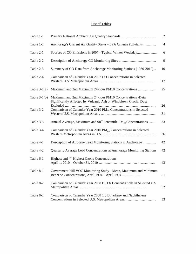
Table 1-1 Primary National Ambient Air Quality Standards ........................................ 2

Table 1-2 Anchorage's Current Air Quality Status - EPA Criteria Pollutants .............. 4

Table 2-1

Sources of CO Emissions in 2007 - Typical Winter Weekday...................... 6

Table 2-2 Description of Anchorage CO Monitoring Sites .......................................... 9

Table 2-3 Summary of CO Data from Anchorage Monitoring Stations (1980-2010)... 10

Table 2-4 Comparison of Calendar Year 2007 CO Concentrations in Selected Western U.S. Metropolitan Areas ……………............................................

17

Table 3-1(a) Maximum and 2nd Maximum 24-hour PM10 Concentrations …………….

.. 25

Table 3-1(b) Maximum and 2nd Maximum 24-hour PM10 Concentrations -Data Significantly Affected by Volcanic Ash or Windblown Glacial Dust Excluded .…………………………………………………….…….........…

26 Table 3-2 Comparison of Calendar Year 2010 PM10 Concentrations in Selected

Western U.S. Metropolitan Areas . …….......................................................

31

Table 3-3 Annual Average, Maximum and 98th Percentile PM2.5Concentrations …… 33

Table 3-4 Comparison of Calendar Year 2010 PM2.5 Concentrations in Selected Western Metropolitan Areas in U.S. …….....................................................

36

Table 4-1 Description of Airborne Lead Monitoring Stations in Anchorage ............... 42

Table 4-2 Quarterly Average Lead Concentrations at Anchorage Monitoring Stations 42

Table 6-1 Highest and 4th Highest Ozone Concentrations

April 1, 2010 – October 31, 2010 …….…………………………..………. 43

Table 8-1 Government Hill VOC Monitoring Study - Mean, Maximum and Minimum Benzene Concentrations, April 1994 – April 1994.....….............

51

Table 8-2 Comparison of Calendar Year 2008 BETX Concentrations in Selected U.S.

Metropolitan Areas ………………………………………………..…

52

Table 8-2 Comparison of Calendar Year 2008 1,3 Butadiene and Naphthalene Concentrations in Selected U.S. Metropolitan Areas………………………

53

vi

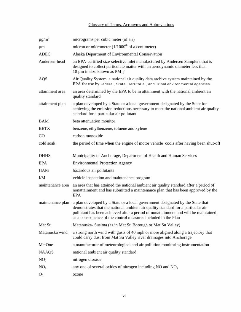
Glossary of Terms, Acronyms and Abbreviations

µg/m3 micrograms per cubic meter (of air)

µm micron or micrometer (1/1000th of a centimeter)

ADEC Alaska Department of Environmental Conservation

Andersen-head an EPA-certified size-selective inlet manufactured by Andersen Samplers that is designed to collect particulate matter with an aerodynamic diameter less than 10 µm in size known as PM10

.

AQS Air Quality System, a national air quality data archive system maintained by the EPA for use by Federal, State, Territorial, and Tribal environmental agencies.

attainment area an area determined by the EPA to be in attainment with the national ambient air quality standard

attainment plan a plan developed by a State or a local government designated by the State for achieving the emission reductions necessary to meet the national ambient air quality standard for a particular air pollutant

BAM beta attenuation monitor

BETX benzene, ethylbenzene, toluene and xylene

CO carbon monoxide

cold soak the period of time when the engine of motor vehicle cools after having been shut-off

DHHS Municipality of Anchorage, Department of Health and Human Services

EPA Environmental Protection Agency

HAPs hazardous air pollutants

I/M vehicle inspection and maintenance program

maintenance area an area that has attained the national ambient air quality standard after a period of nonattainment and has submitted a maintenance plan that has been approved by the EPA

maintenance plan a plan developed by a State or a local government designated by the State that demonstrates that the national ambient air quality standard for a particular air pollutant has been achieved after a period of nonattainment and will be maintained as a consequence of the control measures included in the Plan

Mat Su Matanuska- Susitna (as in Mat Su Borough or Mat Su Valley)

Matanuska wind a strong north wind with gusts of 40 mph or more aligned along a trajectory that could carry dust from Mat Su Valley river drainages into Anchorage

MetOne a manufacturer of meteorological and air pollution monitoring instrumentation

NAAQS national ambient air quality standard

NO2 nitrogen dioxide

NOx any one of several oxides of nitrogen including NO and NO2

O3 ozone

vii

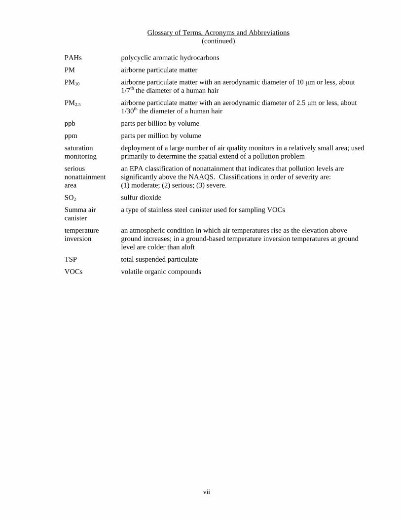
Glossary of Terms, Acronyms and Abbreviations (continued)

PAHs polycyclic aromatic hydrocarbons

PM airborne particulate matter

PM10 airborne particulate matter with an aerodynamic diameter of 10 μm or less, about 1/7th the diameter of a human hair

PM2.5 airborne particulate matter with an aerodynamic diameter of 2.5 μm or less, about 1/30th the diameter of a human hair

ppb parts per billion by volume

ppm parts per million by volume

saturation monitoring

deployment of a large number of air quality monitors in a relatively small area; used primarily to determine the spatial extend of a pollution problem

serious nonattainment area

an EPA classification of nonattainment that indicates that pollution levels are significantly above the NAAQS. Classifications in order of severity are: (1) moderate; (2) serious; (3) severe.

SO2 sulfur dioxide

Summa air canister

a type of stainless steel canister used for sampling VOCs

temperature inversion

an atmospheric condition in which air temperatures rise as the elevation above ground increases; in a ground-based temperature inversion temperatures at ground level are colder than aloft

TSP total suspended particulate

VOCs volatile organic compounds

1

Section 1 - Introduction Purpose of this Report

The purpose of this report is to summarize air quality monitoring data collected in Anchorage since 1980. It focuses on the six pollutants for which the Environmental Protection Agency (EPA) has established a National Ambient Air Quality Standard (NAAQS). They are carbon monoxide, airborne particulate, airborne lead, sulfur dioxide, ozone and nitrogen dioxide.* These pollutants are known as criteria pollutants because a health-based air quality standard has been established for them. National standards for other air pollutants have not been established. This report summarizes criteria pollutant monitoring data in Anchorage and describes the trends observed in the data. In addition to the criteria pollutants, the report also discusses volatile organic compound monitoring data collected from monitoring studies completed in 1994, 1996, 2002 and 2009.

This summary report was originally released in April 1994 and has been updated periodically since then. This updated report includes air quality data collected through December 2010.

National Ambient Air Quality Standards

The Clean Air Act requires the EPA to set National Ambient Air Quality Standards for pollutants considered harmful to public health and the environment. The Clean Air Act established two types of national air quality standards. Primary standards set limits to protect public health, including the health of sensitive populations such as asthmatics, children, and the elderly. Secondary standards set limits to protect public welfare, including protection against decreased visibility, damage to animals, crops, vegetation, and buildings.

The EPA Office of Air Quality Planning and Standards has set a NAAQS for six principal pollutants, which are called criteria pollutants. They are listed below. Units of measure for the standards are parts per million (ppm) by volume, milligrams per cubic meter of air (mg/m3), and micrograms per cubic meter of air (µg/m3).

At five year intervals, the EPA is required to review relevant information and revise standards as necessary.

Anchorage has monitored for air toxics such as benzene that are known for their harmful health effects. There are no ambient standards for these pollutants. These data are summarized in Section 8 of this report.

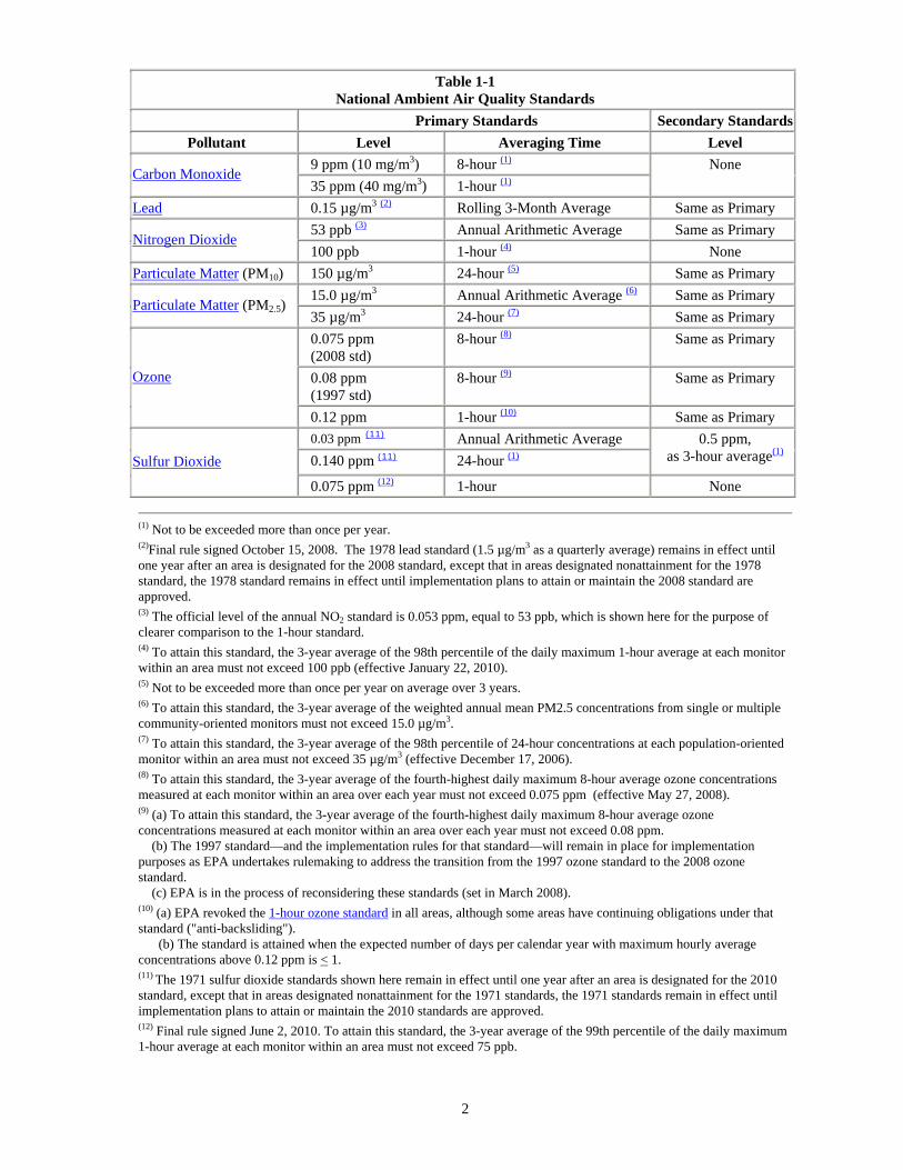
EPA ambient air quality standards for the six criteria pollutants are shown in Table 1-1. This table was adapted from http://epa.gov/air/criteria.html.

* Particulate matter is separated into two size ranges each with a separate NAAQS. Particles, less than 10 microns in diameter are called PM10 and particles less than 2.5 microns in diameter are called PM2.5.

2

Table 1-1 National Ambient Air Quality Standards

Primary Standards Secondary StandardsPollutant Level Averaging Time Level

9 ppm (10 mg/m3) 8-hour (1) Carbon Monoxide

35 ppm (40 mg/m3) 1-hour (1) None

Lead 0.15 µg/m3 (2) Rolling 3-Month Average Same as Primary 53 ppb (3) Annual Arithmetic Average Same as Primary

Nitrogen Dioxide 100 ppb 1-hour (4) None

Particulate Matter (PM10) 150 µg/m3 24-hour (5) Same as Primary 15.0 µg/m3 Annual Arithmetic Average (6) Same as Primary

Particulate Matter (PM2.5) 35 µg/m3 24-hour (7) Same as Primary 0.075 ppm (2008 std)

8-hour (8) Same as Primary

0.08 ppm (1997 std)

8-hour (9) Same as Primary Ozone

0.12 ppm 1-hour (10) Same as Primary 0.03 ppm (11) Annual Arithmetic Average 0.140 ppm (11) 24-hour (1)

0.5 ppm, as 3-hour average(1) Sulfur Dioxide

0.075 ppm (12) 1-hour None

(1) Not to be exceeded more than once per year. (2)Final rule signed October 15, 2008. The 1978 lead standard (1.5 µg/m3 as a quarterly average) remains in effect until one year after an area is designated for the 2008 standard, except that in areas designated nonattainment for the 1978 standard, the 1978 standard remains in effect until implementation plans to attain or maintain the 2008 standard are approved. (3) The official level of the annual NO2 standard is 0.053 ppm, equal to 53 ppb, which is shown here for the purpose of clearer comparison to the 1-hour standard. (4) To attain this standard, the 3-year average of the 98th percentile of the daily maximum 1-hour average at each monitor within an area must not exceed 100 ppb (effective January 22, 2010). (5) Not to be exceeded more than once per year on average over 3 years. (6) To attain this standard, the 3-year average of the weighted annual mean PM2.5 concentrations from single or multiple community-oriented monitors must not exceed 15.0 µg/m3. (7) To attain this standard, the 3-year average of the 98th percentile of 24-hour concentrations at each population-oriented monitor within an area must not exceed 35 µg/m3 (effective December 17, 2006). (8) To attain this standard, the 3-year average of the fourth-highest daily maximum 8-hour average ozone concentrations measured at each monitor within an area over each year must not exceed 0.075 ppm (effective May 27, 2008). (9) (a) To attain this standard, the 3-year average of the fourth-highest daily maximum 8-hour average ozone concentrations measured at each monitor within an area over each year must not exceed 0.08 ppm. (b) The 1997 standard—and the implementation rules for that standard—will remain in place for implementation purposes as EPA undertakes rulemaking to address the transition from the 1997 ozone standard to the 2008 ozone standard. (c) EPA is in the process of reconsidering these standards (set in March 2008). (10) (a) EPA revoked the 1-hour ozone standard in all areas, although some areas have continuing obligations under that standard ("anti-backsliding"). (b) The standard is attained when the expected number of days per calendar year with maximum hourly average concentrations above 0.12 ppm is < 1. (11) The 1971 sulfur dioxide standards shown here remain in effect until one year after an area is designated for the 2010 standard, except that in areas designated nonattainment for the 1971 standards, the 1971 standards remain in effect until implementation plans to attain or maintain the 2010 standards are approved. (12) Final rule signed June 2, 2010. To attain this standard, the 3-year average of the 99th percentile of the daily maximum 1-hour average at each monitor within an area must not exceed 75 ppb.

3

Summary of Anchorage Air Quality Attainment Status and Trends Carbon Monoxide

In 2003, the Municipal Department of Health and Human Services (DHHS) prepared a CO maintenance plan that demonstrates that Anchorage should remain in compliance through at least 2023. After approving the Plan in June 2004, the EPA reclassified Anchorage from a serious carbon monoxide (CO) nonattainment area to a maintenance area. As a maintenance area, Anchorage is now considered in compliance with the CO NAAQS. Anchorage has not violated the CO standard since 1996 and CO concentrations have dropped by approximately 60% from peak levels experienced in the early and mid-1980’s. In 2010, a revised maintenance plan was submitted to EPA that shows that the vehicle inspection and maintenance (I/M) program is no longer necessary to meet the CO NAAQS. The Municipality of Anchorage intends to terminate the I/M program shortly after the EPA approves the revised plan. PM10

The Municipality of Anchorage has experienced exceedances of the NAAQS related to natural events such as volcanic eruptions and wind storms. Experience has shown that the effects of a volcanic eruption can linger for years following the event. During the two-year period following the eruption of the Mt. Spurr volcano in August 1992, the PM10 concentrations exceeded the NAAQS at one or more monitors in Anchorage or Eagle River on 24 days. Intense wind storms in March 2001, March 2003, December 2007 and September 2010 transported large amounts of dust from glacial river valleys in the Matanuska and Susitna Borough that contributed to a number of exceedances of the NAAQS in both Eagle River and the Anchorage bowl. Because these exceedances were the largely the result of natural events, EPA has or will consider excluding them when determining compliance with the PM10 standard.

Although natural events have contributed to some exceedances, most PM10 in Anchorage is believed to have manmade origins. PM10 can be generated from vehicle traffic on unswept roads loaded with winter traction sand or from unpaved roads and parking lots. Anchorage sometimes exceeds the NAAQS during spring break-up especially near heavily traveled roads where traffic stirs up a winter’s worth of accumulated road sand. The most recent exceedance of the standard occurred near Tudor Road in April 2010. Although exceedances have occurred, they have not been numerous enough to constitute a violation of the NAAQS.†

The Municipality of Anchorage and State of Alaska have modified road maintenance practices in an effort to reduce PM10 emissions from roadways. In 1996 they began using a coarser, cleaner traction sand to reduce the amount of fines (silt particles less than 75 microns in diameter) being applied to roadways. In recent years the Municipality of Anchorage has used magnesium chloride brine, a chemical dust suppressant to reduce PM10 emissions during the spring break-up when PM10 concentrations tend to be highest.

Until recently, Eagle River, a community of about 30,000 located approximately 10 miles north of downtown Anchorage, was designated as a nonattainment area for PM10. This designation was the result of air quality violations recorded between 1985 and 1987. A PM10 control plan was developed to address the PM10 problem in Eagle River. Because most of the PM10 in Eagle River was emitted from unpaved roads, this plan focused on paving or surfacing gravel roads in the area. This strategy has been successful. No violations have been measured since October 1987. In 2010 the EPA examined air quality data and determined that Eagle River has in fact attained the NAAQS. A maintenance plan was submitted to the EPA in 2010 that shows that the road surfacing program should continue to provide the PM10 control necessary for continued compliance with the PM10

† According to EPA regulation, a violation occurs when more than three exceedances are experienced in a three-year period.

4

standard. It is currently under EPA review. Once approved, Eagle River will be redesignated as a maintenance area.

PM2.5

Monitoring data collected between 1999 and 2010 indicate that Anchorage is in compliance with the NAAQS for PM2.5. Concentrations measured have been well under the NAAQS. In their 2011 State of the Air report, the American Lung Association ranked Anchorage as the sixth cleanest city in the U.S. for year-round particle (PM2.5) pollution. Lead, Sulfur Dioxide, Ozone, and Nitrogen Dioxide

Airborne lead concentrations in Anchorage dropped dramatically in the 1980’s as lead was phased out of the gasoline supply. By 1987, Anchorage was well below the NAAQS for lead. EPA established a much more stringent air quality standard in 2008, however. Because monitoring for lead has not been performed in recent years, it is not known whether Anchorage meets this new standard.

Monitoring indicates that ground-level ozone levels in the Municipality of Anchorage are well below the NAAQS. Most of the ozone in Anchorage is believed to be naturally occurring. The climate in Anchorage does not appear to be conducive to ozone formation from manmade pollutants.

Although monitoring data for sulfur dioxide (SO2), and nitrogen dioxide (NO2) are limited, the data suggest that Anchorage is likely well under the NAAQS for these two criteria pollutants.

Air Toxics

Because there are no ambient air quality standards for air toxic pollutants, the EPA does not assign attainment/nonattainment status. Monitoring data indicate that ambient concentrations of some air toxics such as benzene are higher in Anchorage than most of the U.S. Concentrations of benzene and other motor vehicle–related air toxics in Anchorage appear to be declining over time, however.

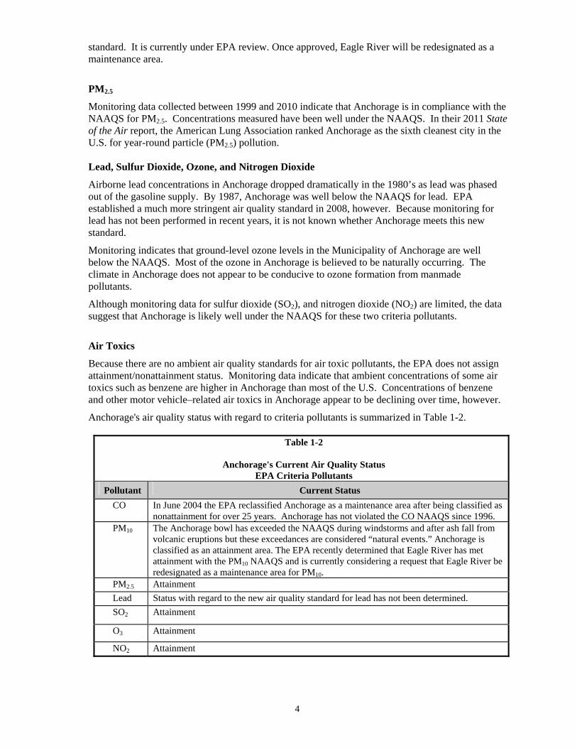
Anchorage's air quality status with regard to criteria pollutants is summarized in Table 1-2.

Table 1-2

Anchorage's Current Air Quality Status EPA Criteria Pollutants

Pollutant Current Status CO In June 2004 the EPA reclassified Anchorage as a maintenance area after being classified as

nonattainment for over 25 years. Anchorage has not violated the CO NAAQS since 1996. PM10 The Anchorage bowl has exceeded the NAAQS during windstorms and after ash fall from

volcanic eruptions but these exceedances are considered “natural events.” Anchorage is classified as an attainment area. The EPA recently determined that Eagle River has met attainment with the PM10 NAAQS and is currently considering a request that Eagle River be redesignated as a maintenance area for PM10.

PM2.5 Attainment Lead Status with regard to the new air quality standard for lead has not been determined. SO2 Attainment

O3 Attainment

NO2 Attainment

5

Section 2 - Carbon Monoxide Health Effects of Carbon Monoxide

Carbon monoxide is a colorless, odorless and poisonous gas produced by incomplete burning of carbon in fuel. The health threat from CO is most serious for those who suffer from cardiovascular disease. A number of studies have suggested that exposure to elevated levels of CO in the ambient air can lead to earlier onset of exercise-induced angina (chest pain) among patients with ischemic heart disease. Other possible risk groups include fetuses, young infants, the elderly and those with pre-existing diseases that decrease the availability of oxygen to critical tissues. The NAAQS for CO is set at 35 ppm (parts per million by volume) for a one-hour average and 9 ppm for an eight-hour average, not to be exceeded more than once per year.‡ This health-based standard is intended to protect those most sensitive to the effects of CO exposure. The eight-hour standard is the more restrictive limit.

Extremely high concentrations (above 1,200 ppm) of CO can develop in indoor environments as the result of faulty home heating systems or because of exhaust leaks in motor vehicles and are considered immediately dangerous to life and health.§ At these concentrations, exposure to CO can cause unconsciousness and even death unless the victim is removed from the source and provided with immediate medical care. Such lethal exposures occur only in indoor or enclosed spaces. Outdoor exposures above 20 ppm are rare in Anchorage, and health effects at these concentrations are subtle even among the susceptible population.

Sources of CO

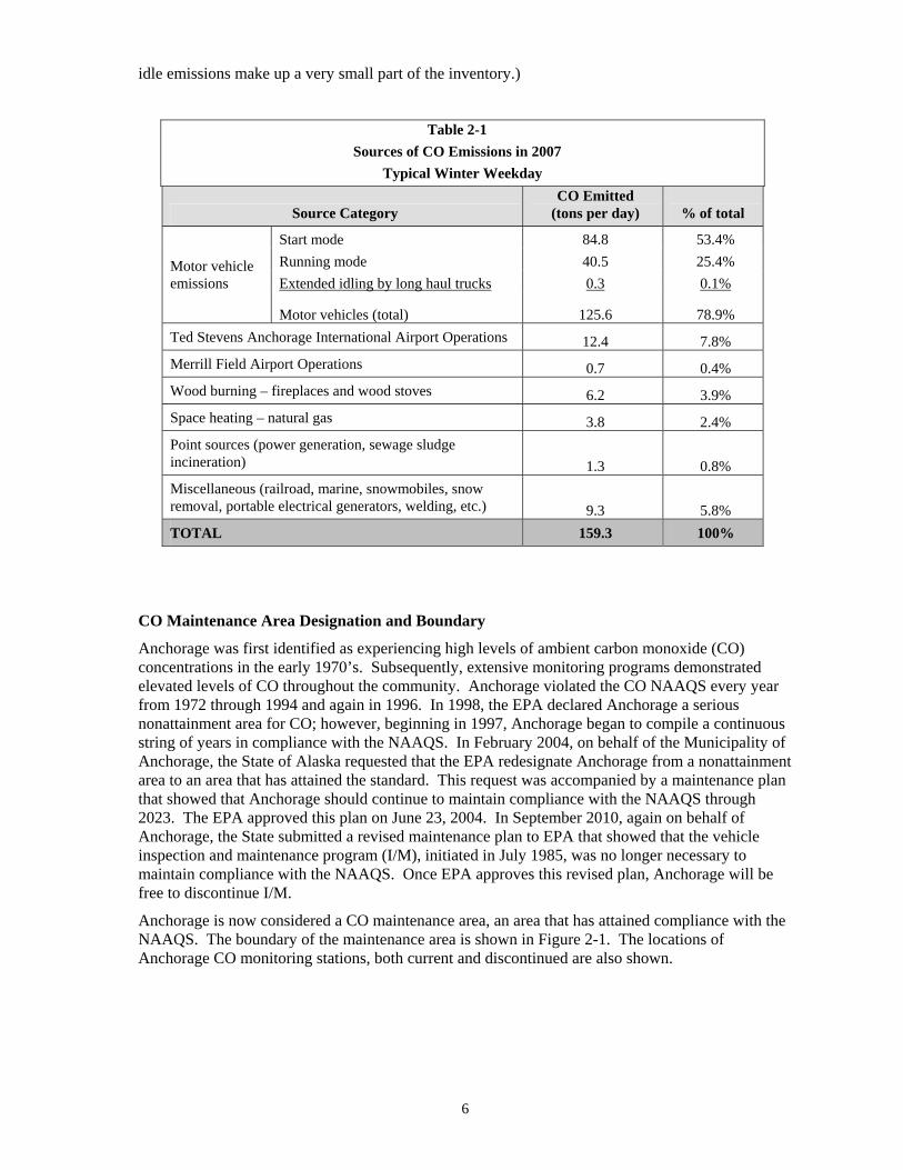
In Anchorage, CO concentrations are highest in mid-winter. According to the latest inventory compiled for the Anchorage bowl area for the year 2007, an estimated 79% of winter season CO emissions in Anchorage were from motor vehicles. Two-thirds of these emissions occur shortly after start-up, especially if the vehicle is cold.** Cold winter temperatures significantly increase CO emissions during the first few minutes of vehicle operation. In the winter, many Anchorage drivers engage in extended warm-ups, particularly prior to a morning commute. A 1998-99 Anchorage study indicated that the average warm-up period for morning commuters was 12 minutes. As a consequence, some of the highest CO concentrations in Anchorage occur in neighborhood residential areas where cold starts and long warm-ups are prevalent.

Other significant sources of CO in Anchorage include airport operations, fireplaces and wood stoves. Estimated CO emissions for a typical winter weekday are summarized by source for the year 2007 in Table 2-1.†† Motor vehicle emissions are broken down into three categories: (1) start; (2) running, and; (3) extended idling by long haul trucks. Start emissions are the “excess emissions” that occur before the engine has reached a fully warm stabilized operating temperature, running emissions are those emissions that occur after warm-up, and extended idle emissions are emissions generated by long haul diesel trucks that are left idling while parked. (These long haul

‡ This standard has been in place for over 30 years. The EPA affirmed this standard on August 31, 2011 after a review of health data.. § National Institute for Occupational Safety and Health (NIOSH) has established the IDHL (immediately dangerous to life and health) for carbon monoxide = 1,200 ppm. ** Estimated with the EPA MOVES model for Anchorage on a winter day with an average temperature of 4 ºF. †† A comprehensive CO inventory was prepared as part of a revised Anchorage CO Maintenance Plan prepared in 2011. Vehicle emissions were estimated using the EPA MOVES emission model in conjunction with vehicle travel estimates from the Anchorage Transportation Model. The FAA EDMS model was used to estimate emissions from Ted Stevens Anchorage International Airport and the EPA NONROAD model was used to estimate emissions from most other source categories.

6

idle emissions make up a very small part of the inventory.)

Table 2-1 Sources of CO Emissions in 2007

Typical Winter Weekday

Source Category CO Emitted

(tons per day)

% of total

Start mode 84.8 53.4% Running mode 40.5 25.4% Extended idling by long haul trucks 0.3 0.1%

Motor vehicle emissions

Motor vehicles (total) 125.6 78.9% Ted Stevens Anchorage International Airport Operations 12.4 7.8% Merrill Field Airport Operations 0.7 0.4% Wood burning – fireplaces and wood stoves 6.2 3.9% Space heating – natural gas 3.8 2.4% Point sources (power generation, sewage sludge incineration) 1.3 0.8% Miscellaneous (railroad, marine, snowmobiles, snow removal, portable electrical generators, welding, etc.) 9.3 5.8% TOTAL 159.3 100%

CO Maintenance Area Designation and Boundary

Anchorage was first identified as experiencing high levels of ambient carbon monoxide (CO) concentrations in the early 1970’s. Subsequently, extensive monitoring programs demonstrated elevated levels of CO throughout the community. Anchorage violated the CO NAAQS every year from 1972 through 1994 and again in 1996. In 1998, the EPA declared Anchorage a serious nonattainment area for CO; however, beginning in 1997, Anchorage began to compile a continuous string of years in compliance with the NAAQS. In February 2004, on behalf of the Municipality of Anchorage, the State of Alaska requested that the EPA redesignate Anchorage from a nonattainment area to an area that has attained the standard. This request was accompanied by a maintenance plan that showed that Anchorage should continue to maintain compliance with the NAAQS through 2023. The EPA approved this plan on June 23, 2004. In September 2010, again on behalf of Anchorage, the State submitted a revised maintenance plan to EPA that showed that the vehicle inspection and maintenance program (I/M), initiated in July 1985, was no longer necessary to maintain compliance with the NAAQS. Once EPA approves this revised plan, Anchorage will be free to discontinue I/M.

Anchorage is now considered a CO maintenance area, an area that has attained compliance with the NAAQS. The boundary of the maintenance area is shown in Figure 2-1. The locations of Anchorage CO monitoring stations, both current and discontinued are also shown.

7

Figure 2-1 Anchorage CO Monitoring Network and Maintenance Boundary

Active sites include Garden Street, Turnagain Boulevard, and 8th & L Street. The Parkgate site in Eagle River is also active but not shown.

CO Monitoring

Over the years, CO monitoring has been conducted at 11 sampling locations in the Municipality of Anchorage. As monitoring priorities have changed, sites have been added and discontinued. In 2010 monitoring was conducted in downtown Anchorage station at 8th and L Street, at the Turnagain Boulevard station in Spenard, at the Garden Street station in east Anchorage and at the Parkgate Building station in the Eagle River central business district.

DHHS monitors CO 24 hours a day from October 1 through March 31 in conformance with guidelines established in federal regulations. Instruments meet all specifications required by the EPA for ambient CO monitoring and are designated by the EPA as a "reference method" for CO. Calibrations are performed regularly in accordance with EPA guidance and the instrument manufacturer's recommendations. Third party instrument performance audits are conducted by EPA

8

EPA and/or by the ADEC at least once during each CO monitoring season.

Hourly averages of CO levels are provided from each station in the network. These data are uploaded to the DHHS central computer and reviewed and submitted to EPA on a quarterly basis for inclusion in their air quality database known as the Air Quality System (AQS). This database contains criteria pollutant and hazardous air pollutant data from around the U.S.

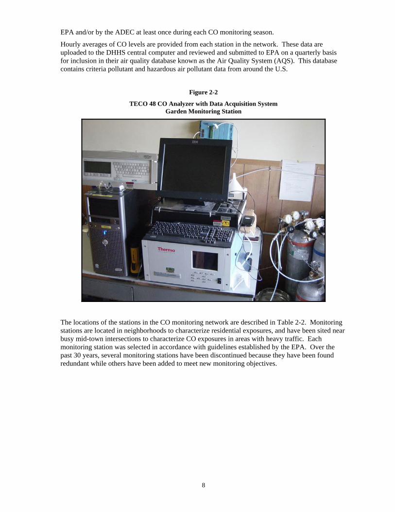
Figure 2-2

TECO 48 CO Analyzer with Data Acquisition System Garden Monitoring Station

The locations of the stations in the CO monitoring network are described in Table 2-2. Monitoring stations are located in neighborhoods to characterize residential exposures, and have been sited near busy mid-town intersections to characterize CO exposures in areas with heavy traffic. Each monitoring station was selected in accordance with guidelines established by the EPA. Over the past 30 years, several monitoring stations have been discontinued because they have been found redundant while others have been added to meet new monitoring objectives.

9

Table 2-2

Description of Anchorage CO Monitoring Sites

Location Site Description

Garden Street Monitoring began at this neighborhood location at 16th Avenue and Garden Street in 1979 and has continued virtually uninterrupted during winter months for three decades.

Turnagain Boulevard

Monitoring began at this neighborhood station near 30th Avenue and Turnagain Boulevard in October 1998. It was established as a result of a special “saturation” monitoring study conducted in the winter of 1997-98. CO concentrations measured here were the highest of the twenty sites monitored during the study.

Parkgate Monitoring began at this station at the Parkgate Building on the old Glenn Highway in downtown Eagle River in December 2005.

8th & L Street Monitoring began at this station in downtown Anchorage site near 8th Avenue and L Street in October 2007.

7th & C Street (discontinued)

This station was located mid-block between 6th and 7th Avenues on C Street. Monitoring began here in 1973 and was discontinued in 1995.

6th and D Street (discontinued)

Monitoring began at this station, located in the “street canyon” near JC Penny in January 1985 and was discontinued in March 1987.

Spenard & Benson (discontinued)

Monitoring began at this site on the southwest corner of Spenard Road and Benson Boulevard in 1978 and was decommissioned in December 2001.

Sand Lake (discontinued)

Monitoring began at this residentially-oriented site, located on Raspberry Road approximately 0.3 miles east of Jewel Lake Road, in 1980 and was discontinued in March 1998.

Seward Highway (discontinued)

Monitoring began at this site, located on the southwest corner of the intersection of Benson Boulevard and Seward Highway, in October of 1987 and was discontinued December 2004.

Jewel Lake (discontinued)

Monitoring began here at this site near Jewel Lake Road, 100 meters north of Dimond Boulevard in October 2002 and was terminated in March 2004.

Bowman (discontinued)

Monitoring began at this neighborhood-scale station at Bowman Elementary in south Anchorage in December 2005 and was discontinued in March 2007.

CO Data Summary and Trends

In 1983, CO levels in Anchorage exceeded the NAAQS at one or more monitoring stations on 53 days. CO concentrations have fallen dramatically over the past twenty years, however. No violations have been measured since 1996. Single exceedances of the NAAQS were measured in 1998, 1999 and 2001 but these were not considered violations because the NAAQS allows up to one exceedance per calendar year. No exceedances were measured in 1995, 1997, 2000, or during the years 2002 through 2010.

Table 2-3 shows the highest and second highest 8-hour averages for seven Anchorage monitoring stations. These values are tabulated along with the number of days exceeding the NAAQS (# days ≥ 9.5 ppm) at each station. Dramatic reductions in CO have occurred between 1980 and 2010. Data from the site where the highest first or second maximum concentration, or greatest number of exceedances occurred in each year are highlighted in yellow. The Spenard & Benson site generally experienced the highest concentrations in the monitoring network until the Seward Highway site commenced operations in 1987. It was surpassed by the Turnagain Boulevard station in residential Spenard when it began operation late in 1998.

10

max

8-h

r

2nd

max

8-h

r

# da

ys ?

9.5

ppm

max

8-h

r

2nd

max

8-h

r

# da

ys ?

9.5

ppm

max

8-h

r

2nd

max

8-h

r

# da

ys ?

9.5

ppm

max

8-h

r

2nd

max

8-h

r

# da

ys ?

9.5

ppm

max

8-h

r

2nd

max

8-h

r

# da

ys ?

9.5

ppm

max

8-h

r

2nd

max

8-h

r

# da

ys ?

9.5

ppm

max

8-h

r

2nd

max

8-h

r

# da

ys ?

9.5

ppm

1980 27.4 26.3 39 17.1 16.8 21 14.0 14.0 61981 17.6 16.3 33 12.6 11.3 7 12.6 11.0 51982 21.6 18.1 30 15.6 13.9 14 16.6 11.9 31983 20.3 16.0 48 19.6 18.0 24 11.5 11.4 71984 17.3 17.1 27 13.0 12.9 7 12.6 11.6 51985 12.6 12.4 9 12.7 12.2 4 9.2 8.9 01986 12.4 11.7 5 10.5 8.8 1 8.1 7.6 01987 9.8 8.6 1 10.7 9.5 1 8.1 6.3 0 11.7 11.5 41988 11.4 10.4 3 11.8 10.5 2 8.5 8.4 0 12.3 11.8 91989 9.8 9.6 2 14.0 9.8 2 10.0 8.4 1 14.0 12.3 51990 9.5 9.4 1 9.8 9.0 1 8.8 8.0 0 13.0 11.6 111991 9.5 8.1 0 8.9 8.4 0 6.7 6.4 0 11.5 9.9 31992 9.0 8.8 0 10.9 10.8 2 7.1 7.0 0 10.4 9.5 21993 8.2 7.7 0 10.0 9.7 2 8.8 5.1 0 10.4 9.9 21994 8.4 8.3 0 9.4 8.6 0 5.8 5.7 0 11.3 11.0 21995 9.2 7.6 0 8.4 7.4 0 6.7 6.3 0 9.0 8.4 01996 11.0 9.6 3 8.9 8.7 0 7.7 6.9 0 10.8 10.5 31997 7.1 6.8 0 7.3 7.1 0 5.9 4.9 0 7.3 7.0 01998 9.3 8.3 0 9.5 7.8 1 6.5 6.1 0 9.4 7.1 0 8.1 7.7 01999 6.6 5.9 0 8.2 7.8 0 7.5 6.5 0 10.1 7.6 12000 5.2 4.7 0 5.8 5.4 0 5.2 4.8 0 7.2 5.5 02001 6.2 5.7 0 6.1 5.7 0 5.4 5.2 0 9.8 7.7 12002 5.3 4.7 0 4.4 4.2 0 6.5 5.9 02003 6.1 5.7 0 6.2 4.9 0 8.3 5.4 02004 6.8 6.4 0 5.8 5.5 0 8.1 7.9 02005 4.8 4.8 0 5.7 4.6 02006 5.1 4.3 0 6.5 6.1 0 3.6 3.6 02007 4.0 3.6 0 5.5 5.0 0 5.4 3.2 0 3.1 2.9 02008 4.1 3.8 0 6.4 5.5 0 3.1 2.9 0 3.8 3.1 02009 5.1 4.4 0 6.1 5.8 0 3.5 3.2 0 3.9 3.6 02010 4.6 3.8 0 6.9 6.0 0 2.7 2.5 0 2.9 2.8 0

Table 2-3

Summary of CO Data from Municipality of Anchorage Monitoring Stations 1980-2010(concentrations in ppm)

SewardHwy

TurnagainBlvd Parkgate

8th and L Street

Spenard & Benson Garden Street

RaspberryRoad

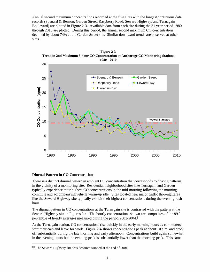
The trend in the second highest 8-hour average concentration or second maximum measured in each calendar year is often used to measure improvements in CO air quality and progress toward attainment of the NAAQS. The second maximum is statistically more robust (i.e., less prone to year-to-year fluctuation) than the first maximum, making it easier to discern long-term air quality trends. The second maximum is also a direct measure of compliance with the NAAQS. A community is considered to be in compliance if the second maximum at all monitoring stations is below 9.5 ppm.

11

Annual second maximum concentrations recorded at the five sites with the longest continuous data records (Spenard & Benson, Garden Street, Raspberry Road, Seward Highway, and Turnagain Boulevard) are plotted in Figure 2-3. Available data from each site during the 31 year period 1980 through 2010 are plotted. During this period, the annual second maximum CO concentration declined by about 74% at the Garden Street site. Similar downward trends are observed at other sites.

Figure 2-3 Trend in 2nd Maximum 8-hour CO Concentration at Anchorage CO Monitoring Stations

1980 - 2010

0

5

10

15

20

25

30

1980 1985 1990 1995 2000 2005 2010

CO

Con

cent

ratio

n (p

pm)

Spenard & Benson Garden Street

Raspberry Road Seward Hwy

Turnagain Blvd

Federal Standard

Diurnal Pattern in CO Concentrations

There is a distinct diurnal pattern in ambient CO concentration that corresponds to driving patterns in the vicinity of a monitoring site. Residential neighborhood sites like Turnagain and Garden typically experience their highest CO concentrations in the mid-morning following the morning commute and accompanying vehicle warm-up idle. Sites located near major traffic thoroughfares like the Seward Highway site typically exhibit their highest concentrations during the evening rush hour.

The diurnal pattern in CO concentrations at the Turnagain site is contrasted with the pattern at the Seward Highway site in Figures 2-4. The hourly concentrations shown are composites of the 99th percentile of hourly averages measured during the period 2001-2004.‡‡

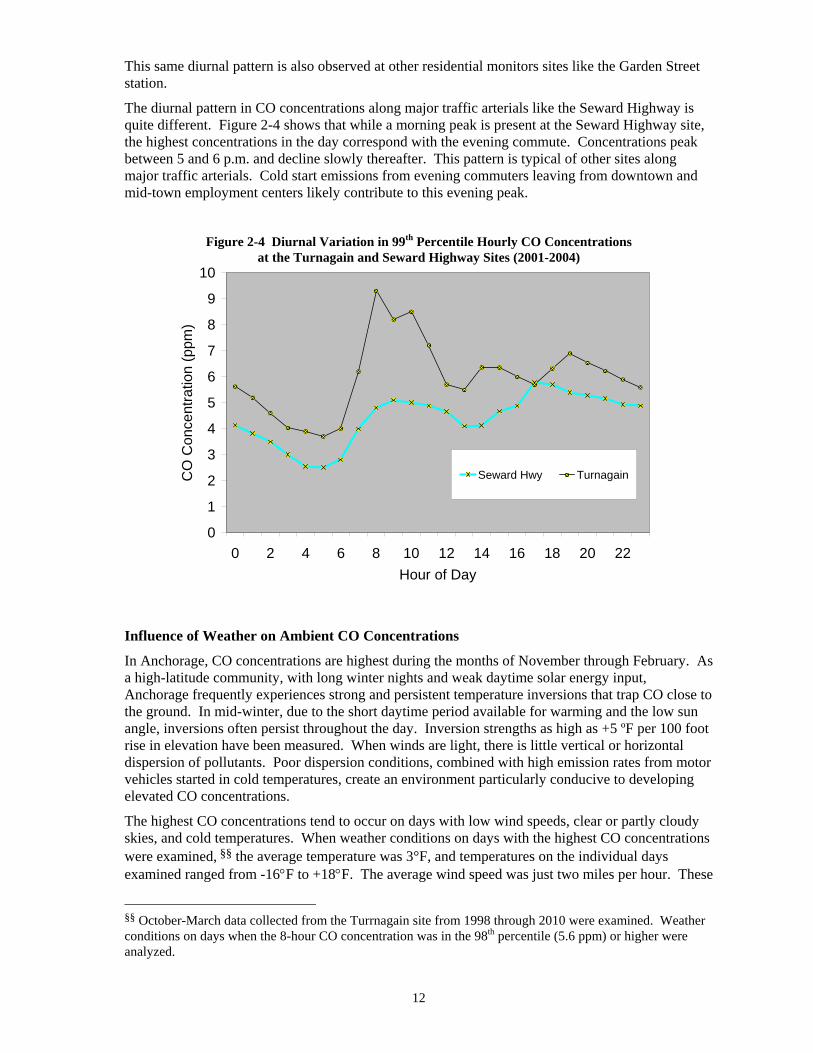
At the Turnagain station, CO concentrations rise quickly in the early morning hours as commuters start their cars and leave for work. Figure 2-4 shows concentrations peak at about 10 a.m. and drop off substantially during the late morning and early afternoon. Concentrations build again somewhat in the evening hours but the evening peak is substantially lower than the morning peak. This same ‡‡ The Seward Highway site was decommissioned at the end of 2004.

12

This same diurnal pattern is also observed at other residential monitors sites like the Garden Street station.

The diurnal pattern in CO concentrations along major traffic arterials like the Seward Highway is quite different. Figure 2-4 shows that while a morning peak is present at the Seward Highway site, the highest concentrations in the day correspond with the evening commute. Concentrations peak between 5 and 6 p.m. and decline slowly thereafter. This pattern is typical of other sites along major traffic arterials. Cold start emissions from evening commuters leaving from downtown and mid-town employment centers likely contribute to this evening peak.

Figure 2-4 Diurnal Variation in 99th Percentile Hourly CO Concentrations at the Turnagain and Seward Highway Sites (2001-2004)

0

1

2

3

4

5

6

7

8

9

10

0 2 4 6 8 10 12 14 16 18 20 22Hour of Day

CO

Con

cent

ratio

n (p

pm)

Seward Hwy Turnagain

Influence of Weather on Ambient CO Concentrations

In Anchorage, CO concentrations are highest during the months of November through February. As a high-latitude community, with long winter nights and weak daytime solar energy input, Anchorage frequently experiences strong and persistent temperature inversions that trap CO close to the ground. In mid-winter, due to the short daytime period available for warming and the low sun angle, inversions often persist throughout the day. Inversion strengths as high as +5 ºF per 100 foot rise in elevation have been measured. When winds are light, there is little vertical or horizontal dispersion of pollutants. Poor dispersion conditions, combined with high emission rates from motor vehicles started in cold temperatures, create an environment particularly conducive to developing elevated CO concentrations.

The highest CO concentrations tend to occur on days with low wind speeds, clear or partly cloudy skies, and cold temperatures. When weather conditions on days with the highest CO concentrations were examined, §§ the average temperature was 3°F, and temperatures on the individual days examined ranged from -16°F to +18°F. The average wind speed was just two miles per hour. These

§§ October-March data collected from the Turrnagain site from 1998 through 2010 were examined. Weather conditions on days when the 8-hour CO concentration was in the 98th percentile (5.6 ppm) or higher were analyzed.

13

per hour. These high CO periods almost always occurred during periods with clear skies or scattered cloud cover, conditions that are conducive to the development of radiative temperature inversions. Radiative temperature inversions tend to occur when skies are clear or partly cloudy because under these conditions, heat stored by the ground is radiated toward space, cooling the ground surface which in turn cools the air layer immediately above it. The result of this cooling is a shallow but strong ground-based temperature inversion that traps pollutants near ground-level. These shallow inversions usually develop after sunset when there is no solar heating. They tend to erode after sunrise when solar energy begins to heat the ground. In the winter, Anchorage and other high latitude Alaska communities likely experience more persistent temperature inversions than in the lower-48 because sunset occurs earlier, sunrise occurs later, and the solar energy received during the day is weaker.

Role of Mechanical Turbulence from Vehicle Traffic in Reducing Ambient CO Concentrations during Stagnation Conditions

As noted earlier, the highest CO concentrations in Anchorage tend to occur in residential neighborhoods rather than near major roadways where vehicle traffic volumes may be an order of magnitude greater. If the ambient CO concentration in a particular area were solely a function of the quantity of emissions produced there, CO concentrations near major roadways in midtown Anchorage should be higher than residential areas. Although average CO concentrations along major roadways are higher than residential areas, the highest CO concentrations occur in residential areas rather than along roadways. Ambient monitoring data show that when severe stagnation conditions occur and there is very little natural atmospheric mixing, the highest CO concentrations can be found in residential areas.

Monitoring data suggest that mechanical mixing from high-speed vehicle traffic reduce ambient CO concentrations near major traffic thoroughfares on severe stagnation days. When a strong ground-based temperature inversion and lack of wind create very poor natural atmospheric mixing, mechanical mixing from vehicle traffic appears to be a very important factor in mitigating the build up of high CO concentrations. Under these extreme meteorological conditions concentrations at Turnagain are much higher than those at Seward Highway. On the very highest CO days, when CO concentrations are in the 99th percentile, concentrations at the Turnagain monitor are roughly 40% higher than the Seward Highway station. In contrast, on a typical day, as reflected by the median concentration, concentrations at Turnagain are about 30% lower than the Seward Highway. This suggests that turbulence from higher speed traffic along major traffic corridors helps to disperse CO emissions and reduce concentrations especially when natural atmospheric mixing is constrained by lack of wind and/or a temperature inversion.

Summary of Local Research

Beginning in 1997, the MOA in cooperation with the EPA, ADEC and the Fairbanks North Star Borough, conducted a number of studies to advance the understanding of the causes of the winter season CO problem in Anchorage and Fairbanks. In particular, these studies focused on quantifying the contribution of cold starts and warm up idling on the problem. These studies are summarized below.

1997 – 1998 CO Saturation Monitoring Study

The MOA performed additional CO monitoring during the period December 4, 1997 - February 4, 1998. Sixteen temporary monitoring sites were established to assess how well the four station permanent network was characterizing the air quality near congested roadway intersections, in neighborhoods and in parking lots. Monitoring was conducted at 20 locations during the study period. Eight sites were located near major roadway intersections, seven in neighborhoods, and five

14

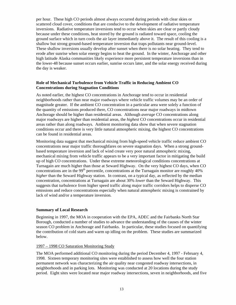
five in large retail or employee parking lots. The maximum eight-hour concentrations measured at each of the 20 sites in the study are compared in Figure 2-5. (Sites noted in all caps were permanent monitoring stations; others were temporary.)

Figure 2-5 Maximum 8-hour CO Concentrations Measured during CO Saturation Monitoring Study

The highest eight-hour CO concentrations were found at neighborhood locations with relatively low traffic volumes. The Turnagain neighborhood site recorded the highest and second highest eight-hour concentrations in the study. The next highest site was the Garden permanent station, also located in a neighborhood. Vehicle cold starts and warm-up idling by morning commuters were implicated as the cause of the elevated CO observed in these neighborhoods.

The permanent station at Seward Highway recorded the highest concentration of any of the eight roadway intersection sites. The study concluded that the Seward Highway station adequately characterized the upper range of CO concentrations experienced near major roadways in Anchorage. Lower than expected concentrations were found near a number of congested intersections. For example, the highest concentration measured near the busy intersection of Lake Otis Boulevard and Tudor Road was about 50% lower than the Turnagain neighborhood site.

CO concentrations at the five parking lot sites were generally lower than those found in neighborhoods or near the major roadway intersections monitored during the study. This was somewhat surprising given the number of vehicle start-ups that originated in these parking lots. Many of these start ups, especially in retail shopping parking lots, were likely to be “hot starts,” however, meaning that engines were still warm from an earlier trip. Warmer engines emit considerably lower amounts of CO and this may account for the relatively low ambient concentrations observed.

15

Anchorage Winter Season Driver Idling Behavior Study (1997-98)

DHHS conducted a study between November 28, 1997 and January 31, 1998 aimed at quantifying the amount of warm up idling performed by Anchorage drivers. Field staff observed 1,321 vehicle starts at diverse locations in Anchorage. Warm-up idling duration was documented for trips that began at homes, work places, and other locations such as shopping centers, restaurants, and schools.

Field observations were used to estimate idle duration for each of the trip purpose categories described above. The longest warm-up idle times were associated with morning commute trips to work. The average idle duration for these trips for cars parked outside was about 12 minutes***. The average idle duration for evening commute trips beginning at the workplace was 3.4 minutes. The shortest idle durations were associated with morning and midday trips that began at sites other than work or home. Median idle time for these trips was less than one minute.

Engine soak times, the length of time that an engine sits in the cold between trips, were also estimated as part of the driver idling behavior study. Longer soak times result in colder engines and increased CO emissions. Data from a travel survey conducted by Hellenthal and Associates for the municipality in 1992, were used to estimate soak times by trip purpose and time of day.

The longest soak times and idle durations were associated with morning home-based work trips. Because most of these trips begin with a cold engine and involve long idles, start up and idle CO emissions are likely to be greater than other trip types. Conversely, non work-related trips originating from shopping centers, health clubs and similar non work-related locations typically involve short soak times and idle durations, and are therefore likely to have lower start up and idle emissions.

Alaska Cold Start and Idle Emissions Studies (Winter 1998-99 and Winter 2000-2001)

During the winter of 1998-99, Sierra Research conducted a study to quantify emissions from Alaskan vehicles during cold start and idling. This testing, which was coordinated jointly by the MOA, Fairbanks Northstar Borough and ADEC, measured emissions under winter conditions when the highest CO concentrations are likely to occur. Sierra Research equipped a large van with a modified Horiba IMVETS emissions test system that provided measurements of CO and hydrocarbon mass emissions on a second-by-second basis. The van could be driven from location to location to test a variety of vehicles representative of the fleet mix in both Anchorage and Fairbanks.

After an initial cold soak of four hours or more at ambient temperature, test vehicles were cold-started and mass emissions were measured for a period of 20 minutes subsequent to start-up. Testing was conducted at ambient temperatures that ranged from -6 °F to +23 °F in Anchorage and -36 °F to +14 °F in Fairbanks. The data collected during the study were used to help estimate idle emissions in the CO emissions inventories compiled for 1996 and 2000.

Sierra Research conducted a follow-up study in Fairbanks during the winter of 2000-2001. During this study, mass emission testing was conducted using a dynamometer which allowed emissions to be tested during a simulated, representative urban Alaska trip (i.e. varying speeds, accelerations, stops). Key findings from the 1998-99 and 2000 –2001 studies are summarized below:

*** About 35% of morning trips involved vehicles parked overnight in heated garages. Idle duration for these vehicles averaged less than one minute. The average idle duration for vehicles parked outside was over 12 minutes. The weighted average idle duration for all work-related morning trips, including those originating from a garage was about 7 minutes.

16

• A large portion of CO emissions occur during cold start and warm-up idle. In order to simulate a typical morning commute in Anchorage†††, Sierra Research measured CO emissions from 35 cold-started vehicles during the course of a 10-minute warm-up and a subsequent 7.3-mile drive. The CO emitted during cold start and warm-up idle made up 68% of the total CO emitted. More than two-thirds of the CO emissions generated by Anchorage’s morning commuters may occur before their vehicles even leave home.

• To minimize emissions after a cold start, the optimum warm-up idle time is about 10 minutes. On an overall trip basis (10-minute warm-up followed by a 7.3-mile drive), CO emissions actually increase when idle times are cut shorter than 10 minutes. When the idle time is cut to five minutes, overall trip emissions increased by an average of 8%, and by about 20% when the warm-up time was cut to 2 minutes. Warm-ups longer than 10 minutes increase emissions. A 15-minute idle increased emissions by about 10% when compared to a 10-minute idle.

• Using an engine heater prior to a cold start cuts CO emissions dramatically. Plugging in for two hours before a cold start cut emissions during a 10-minute warm-up idle period by an average of 59%. Overall trip emissions were cut by an average of 42%. (See Figure 2-6)

• Turning a warmed up car off when doing short errands provides little or no air quality benefit. Once a vehicle is warmed up, Sierra found that there was no air quality benefit from turning it off during a typical 20, 40 or 60-minute errand. In other words, total CO emissions were about the same whether the vehicle was left running or turned off and then restarted.

• Tailpipe emissions of benzene and other air toxics appear to be closely correlated with CO emissions. Sierra Research’s testing data demonstrated that when CO emissions are high so are emissions of benzene and other air toxics. This suggests that strategies aimed at reducing CO emissions (i.e. plugging in and the vehicle I/M program) also reduce air toxic emissions.

Figure 2-6

Comparison of CO Emissions during 10 Minute Warm-up after Cold Start Plug-in vs. No Plug-in

††† Data collected in Anchorage show that the average warm-up idle time among morning commuters is 12 minutes. The average commute trip is about 7 miles.

17

CO Concentrations in Anchorage Compared with Other Areas

CO data from monitoring stations in the U.S. is archived in the EPA AQS database (http://www.epa.gov/ttn/airs/airsaqs/aqsweb/). Calendar year 2010 data from selected western metropolitan areas are compared with Anchorage in Table 2-4. Concentrations measured in Anchorage were among the highest in the U.S. Data from Anchorage were recorded by the Turnagain monitoring station in residential Spenard.

Comparison of data from different metropolitan areas should be done with caution. CO measurements are highly dependent on proximity to local sources (e.g. road ways, industrial sources) and may not necessarily be representative of area-wide air quality.

Table 2-4

Comparison of Calendar Year 2010 CO Concentrations in

Selected Western U.S. Metropolitan Areas

Metropolitan Area

Highest 8-hour Concentration

(ppm)

2nd Highest 8-hour Concentration

(ppm) Number of Exceedances

of the NAAQS Anchorage, AK 6.9 6.1 0 Fairbanks, AK 5.0 4.1 0 Las Vegas, NV 3.4 3.0 0 Phoenix, AZ 3.3 3.2 0 El Paso, TX 3.3 2.8 0 Denver, CO 3.1 2.4 0 Ogden, UT 2.4 1.9 0 Reno, NV 2.4 2.1 0 Portland, OR 2.4 2.4 0 Spokane, WA 2.3 1.9 0 Salt Lake City, UT 2.2 1.9 0 Albuquerque, NM 2.0 2.0 0 Sacramento, CA 1.9 1.9 0 Seattle, WA 0.8 0.7 0

18

References 1. "Anchorage Carbon Monoxide Maintenance Plan," Air Quality Program, Department of Health and Human Services, Municipality of Anchorage, adopted by the Anchorage Assembly, June 8, 2011.

2. “Anchorage 2007 Carbon Monoxide Emission Inventory and 2007-2023 Attainment Projections,” Air Quality Program, Department of Health and Human Services, Municipality of Anchorage, April 2011.

3. EPA AirData website, Office of Air and Radiation, U.S. Environmental Protection Agency. http://www.epa.gov/air/data/

4. “Air Quality Criteria for Carbon Monoxide,” U.S. Environmental Protection Agency, Office of Research and Development, National Center for Environmental Assessment, Washington, DC, EPA 600/P-99/001F, 2000.

5. “Winter 1997-98 Anchorage Carbon Monoxide Saturation Monitoring Study,” Air Quality Program, Department of Health and Human Services, Municipality of Anchorage, September 1998.

6. “Analysis of Alaska Vehicle CO Emission Study Data,” prepared for the Municipality of Anchorage by Sierra Research, Inc., February 3, 2000.

7. “Fairbanks Cold Temperature Vehicle Testing: Warm-up Idle, Between Trip Idle, and Plug-In,” prepared for the Alaska Department of Environmental Conservation by Sierra Research, Inc., July 2001.

19

Section 3 - Particulate Matter Health Effects of Particulate Matter

Airborne particulate matter is composed of dust, ash, soot, smoke or liquid droplets emitted into the air by industrial sources, fires, construction activities, paved and unpaved roads, and from natural sources like volcanoes and wind blown dust.

Smaller size particulate is most likely to cause adverse health effects. Particles smaller than 10 microns (μm) in diameter, called PM10, can be inhaled into the thoracic regions of the respiratory tract where they can be harmful. Particles smaller than 2.5 μm, called PM2..5 can be inhaled even more deeply into the lungs. Epidemiological studies indicate that adverse health impacts can result from exposure to particulate matter concentrations commonly experienced in many U.S. urban areas. These health impacts include aggravation of existing respiratory disease and decline in lung function. Studies in a number of cities have shown increases in morbidity and mortality when PM2.5 levels are high. Although the evidence regarding adverse health impacts from PM10 exposure is less compelling than PM2.5, some studies have shown an increase in hospital visits when PM10 concentrations rise. In Anchorage, evidence suggests an association between elevated PM10 and increases in out-patient visits for asthma and upper respiratory illness (Gordian 1996, Chimonas 2006).

In September 2007, the EPA revised the NAAQS for particulate. The revised standard includes more stringent limits on fine particulate matter less than 2.5 μm in diameter, called PM2.5. Recent epidemiological studies indicate that adverse health impacts are strongly related to exposure to fine particulate. A growing body of epidemiological evidence suggests that these sub-2.5 μm particles have a greater impact on human health than coarser particles in the 2.5 to 10 μm size range. EPA retained the existing 24-hour NAAQS of 150 μg/m3 but revoked the annual standard previously established at 50 μg/m3 citing a lack of evidence of adverse impacts from long term exposure.

The current EPA annual standard for PM2.5 is 15 μg/m3 and the 24-hour standard, established for the

98th percentile of monitored values, is 35 μg/m3. This means that a community may exceed 35 μg/m3 on up to 2% of the days monitored and still comply with the NAAQS. If monitoring is conducted 365 days per year, this amounts to seven days per year. Compliance with the annual and 24-hour NAAQS are determined by averaging over a three-year period.

The current NAAQS for PM10 is set at 150 μg/m3 as a 24-hour average, not to be exceeded more than

once per year averaged over a three-year period. In 2011, EPA is reviewing the PM standard again. Changes in the level and form of the PM2.5 and PM10 standard are possible.

This chapter is divided into two sections. The first will address PM10, the second PM2.5.

20

PM10 Monitoring

Particulate monitoring of one sort or another has been performed in Anchorage since the 1950’s when “dust bucket” monitoring was conducted by the Public Health Service. In the 1970’s and 80’s total suspended particulate (TSP) monitoring was conducted. In 1985, DHHS began monitoring for PM10 in anticipation of the new PM10 NAAQS which became effective in 1987.

Until recently, DHHS relied largely on Andersen-head PM10 samplers to measure PM10. The Andersen-head sampler has been designated by EPA as a reference method for PM10 measurement and is used commonly throughout the U.S. In short, the method involves placing a pre-weighed quartz fiber filter in an Andersen sampler set to operate for a 24-hour period, from midnight to midnight. The filter is collected after the sampler has run, equilibrated to prescribed conditions in the laboratory, and then weighed again. The PM10 mass is calculated by subtracting the weight of the filter before sampling. Once the PM10 mass is known, the PM10 concentration can be calculated from the sample duration and flow rate through the sampler. Adjustments are made to account for the temperature and barometric pressure on the sample day.

Beginning in 2009, DHHS switched largely to continuous PM10 sampling systems that do not require manual deployment, retrieval and weighing of filters to determine PM10 mass. These continuous systems provide data on an hourly basis to a centralized computer system that can be accessed at any time. DHHS currently uses Met One beta attenuation monitors (BAMs) at all four of the active stations in the network. The BAM draws air in at a known flow rate through a glass fiber filter. A low level beta radiation source in the instrument is directed through the filter where the particulate is deposited. The instrument estimates the mass of the particulate by measuring the attenuation in the beta radiation. A greater the particulate mass results in greater attenuation. The instrument then calculates the PM10 concentration from mass and the flow data. PM10 data from the BAMs are automatically uploaded to the Internet and are accessible to the public at www.anchorageair.info.

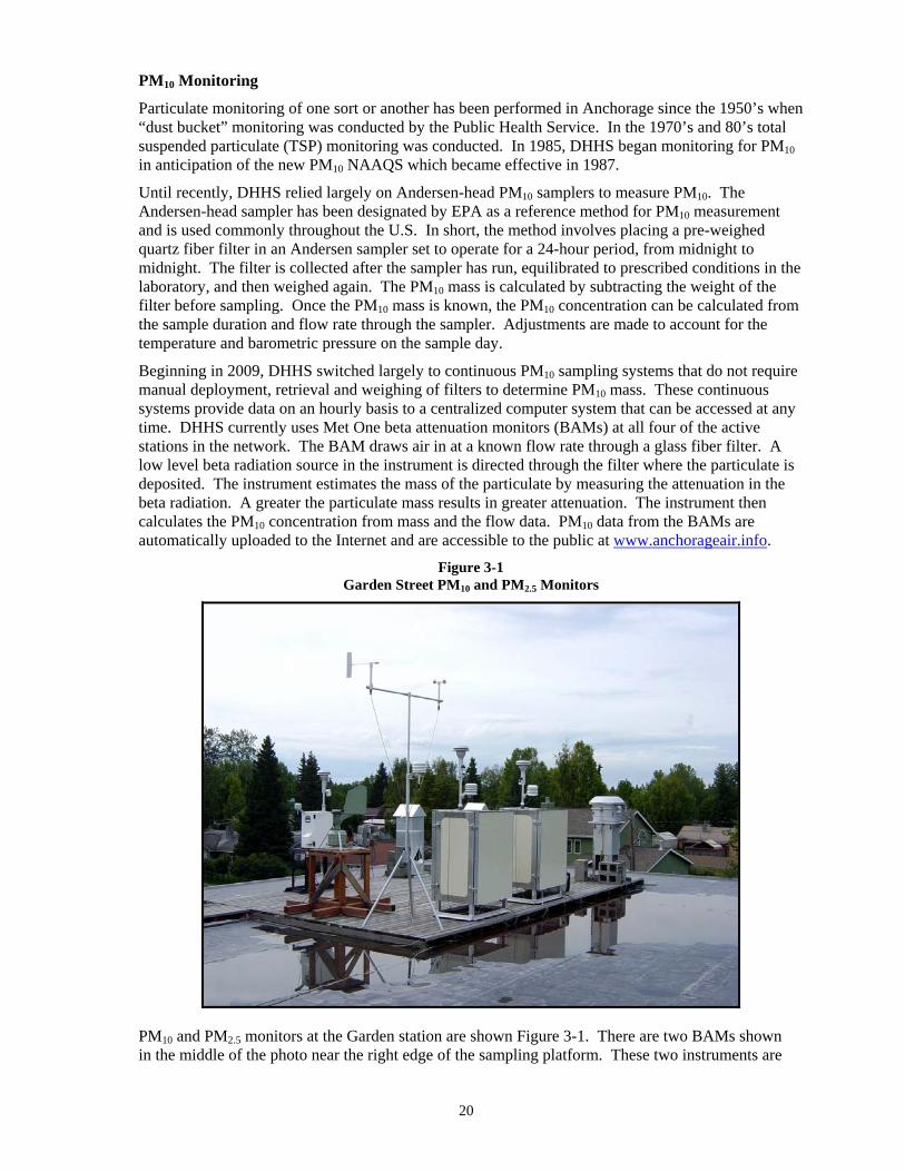
Figure 3-1 Garden Street PM10 and PM2.5 Monitors

PM10 and PM2.5 monitors at the Garden station are shown Figure 3-1. There are two BAMs shown in the middle of the photo near the right edge of the sampling platform. These two instruments are

21

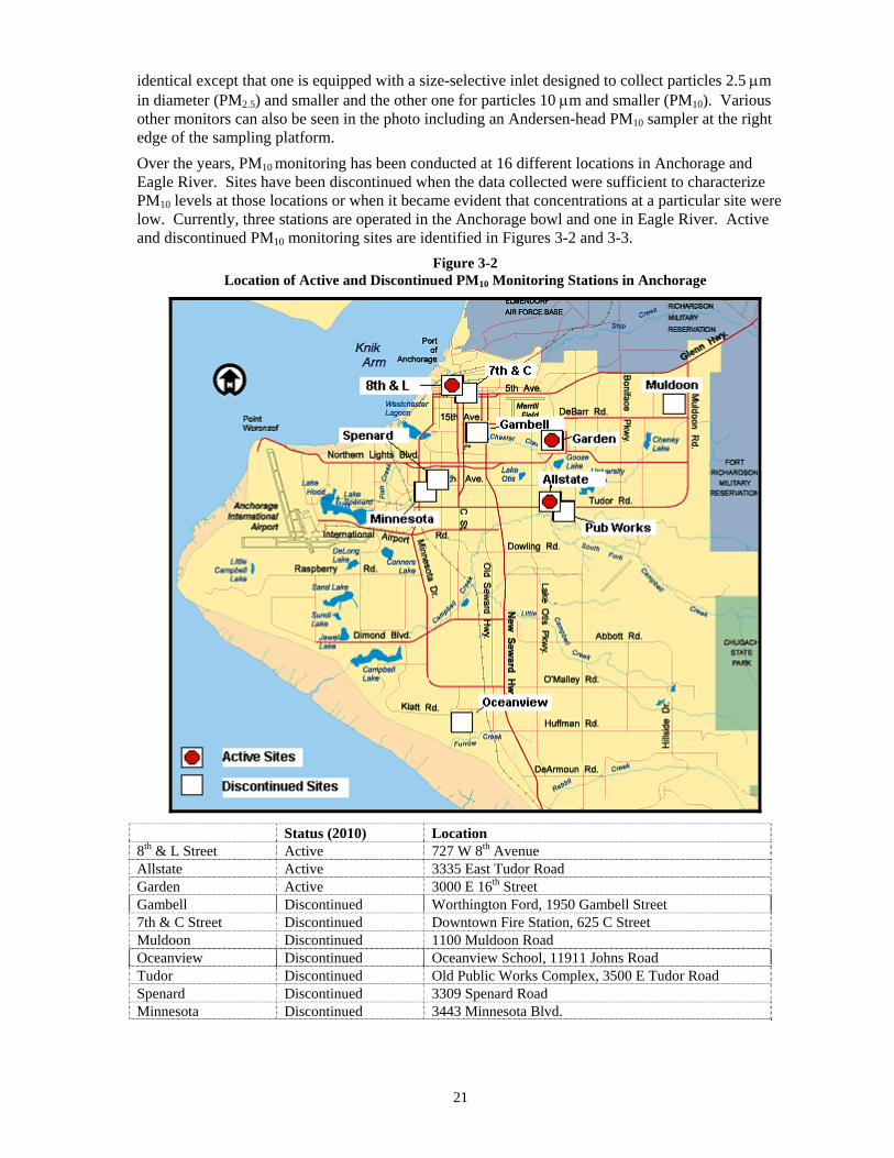
identical except that one is equipped with a size-selective inlet designed to collect particles 2.5 μm in diameter (PM2.5) and smaller and the other one for particles 10 μm and smaller (PM10). Various other monitors can also be seen in the photo including an Andersen-head PM10 sampler at the right edge of the sampling platform. Over the years, PM10 monitoring has been conducted at 16 different locations in Anchorage and Eagle River. Sites have been discontinued when the data collected were sufficient to characterize PM10 levels at those locations or when it became evident that concentrations at a particular site were low. Currently, three stations are operated in the Anchorage bowl and one in Eagle River. Active and discontinued PM10 monitoring sites are identified in Figures 3-2 and 3-3.

Figure 3-2 Location of Active and Discontinued PM10 Monitoring Stations in Anchorage

Status (2010) Location 8th & L Street Active 727 W 8th Avenue Allstate Active 3335 East Tudor Road Garden Active 3000 E 16th Street Gambell Discontinued Worthington Ford, 1950 Gambell Street 7th & C Street Discontinued Downtown Fire Station, 625 C Street Muldoon Discontinued 1100 Muldoon Road Oceanview Discontinued Oceanview School, 11911 Johns Road Tudor Discontinued Old Public Works Complex, 3500 E Tudor Road Spenard Discontinued 3309 Spenard Road Minnesota Discontinued 3443 Minnesota Blvd.

22

Figure 3-3 Location of Active and Discontinued PM10 Monitoring Stations in Eagle River

(with PM10 Nonattainment Boundary shown in Red)

Site Status (2008) Location Parkgate Active Parkgate Bldg., near Old Glenn Hwy &Easy Street Caribou Discontinued Homestead School, 15 meters north of Baranoff Drive AWWU Discontinued AWWU Wastewater facility, Artillery Road Fire Lake Rec Center Discontinued Fire Lake Recreation Center, Mile 2.2, Old Glenn Hwy Homestead Discontinued Homestead School, 50 meters north of Baranof Drive Colville Discontinued AWWU well house, intersection, Baranoff & Colville Streets Eagle River Elementary Discontinued Eagle River Elementary School

23

Sources of PM10 in Anchorage

Sources of PM10 in Anchorage and Eagle River have been quantified by a technique known as chemical mass balance receptor modeling. Over 90% of the PM10 matter is attributed to paved and unpaved roads. The combined impact of other sources, such as emissions from industrial sources, wood stoves and fireplaces, and automobiles amount to less than 10% of the particulate mass.

Unpaved roads were the major source of PM10 in Eagle River prior to 1988. Areas located near unpaved roads with appreciable traffic experienced frequent violation of the NAAQS; however, an ambitious road paving and surfacing program has largely eliminated this source of emissions and air quality has improved.

Effect of Volcanic Eruptions and Glacial River Dust on PM10 in Anchorage and Eagle River

Since PM10 monitoring began in 1985, the 24-hour average concentration measured at various monitoring sites in Anchorage and Eagle River has exceeded the 150 μg/m3 NAAQS on 63 occasions. Over two-thirds (46) are attributed to natural events such as volcanic eruptions or dust transported by high winds from glacial river valleys in the Mat Su Valley north of Anchorage. Anchorage is surrounded by volcanoes to the south and west. Three of these, Mt. Augustine, Redoubt, and Spurr, have erupted at least once in the past twenty five years. In particular, the eruptions of Mt. Redoubt in 1990 and Mt. Spurr in 1992 were responsible for numerous exceedances of the 24-hour NAAQS during the initial ash fall and in the months following as deposited ash was re-entrained by wind and/or traffic along major roadways.

Figure 3-4

Active Cook Inlet Volcanoes, Eruption of Mt. Spurr August 18, 1992

Map and Photo Courtesy of Alaska Volcano Observatory

24

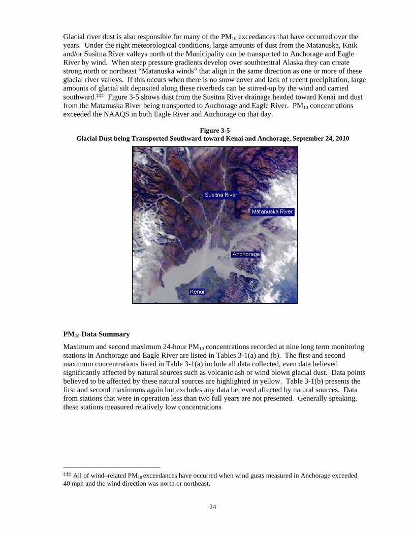
Glacial river dust is also responsible for many of the PM10 exceedances that have occurred over the years. Under the right meteorological conditions, large amounts of dust from the Matanuska, Knik and/or Susitna River valleys north of the Municipality can be transported to Anchorage and Eagle River by wind. When steep pressure gradients develop over southcentral Alaska they can create strong north or northeast “Matanuska winds” that align in the same direction as one or more of these glacial river valleys. If this occurs when there is no snow cover and lack of recent precipitation, large amounts of glacial silt deposited along these riverbeds can be stirred-up by the wind and carried southward.‡‡‡ Figure 3-5 shows dust from the Susitna River drainage headed toward Kenai and dust from the Matanuska River being transported to Anchorage and Eagle River. PM10 concentrations exceeded the NAAQS in both Eagle River and Anchorage on that day.

Figure 3-5

Glacial Dust being Transported Southward toward Kenai and Anchorage, September 24, 2010

PM10 Data Summary

Maximum and second maximum 24-hour PM10 concentrations recorded at nine long term monitoring stations in Anchorage and Eagle River are listed in Tables 3-1(a) and (b). The first and second maximum concentrations listed in Table 3-1(a) include all data collected, even data believed significantly affected by natural sources such as volcanic ash or wind blown glacial dust. Data points believed to be affected by these natural sources are highlighted in yellow. Table 3-1(b) presents the first and second maximums again but excludes any data believed affected by natural sources. Data from stations that were in operation less than two full years are not presented. Generally speaking, these stations measured relatively low concentrations

‡‡‡ All of wind–related PM10 exceedances have occurred when wind gusts measured in Anchorage exceeded 40 mph and the wind direction was north or northeast.

25

Table 3-1(a)

Maximum and 2nd Maximum 24-hour PM10 Concentrations (all values μg/m3)

Anchorage Sites Eagle River Sites

7th&C Garden Gambell Oceanview Muldoon Allstate DHHS Caribou* Parkgate 1986 115 / 108 --- --- --- --- --- --- --- 336 / 326 1987 63 / 59 --- --- --- --- --- --- --- 219 / 147 1988 47 / 46 --- 134 / 132 --- --- --- --- --- 83 / 83 1989 63 / 41 --- 137 / 104 --- --- --- --- 108 / 106 69 / 56 1990 108 / 94 --- 260 / 188 81 / 77 --- --- --- 101 / 83 143 / 106 1991 --- --- 144 / 141 130 / 99 --- --- --- 180 / 148 78 / 72 1992 --- --- 565 / 446 549 / 331 --- --- --- 304 / 170 165 / 128 1993 --- --- 185 / 174 123 / 69 --- --- --- 71 / 66 79 / 77 1994 --- --- 242 / 198 84 / 79 --- --- --- 90 / 66 94 / 60 1995 --- --- 206 / 192 147 / 102 116 / 89 --- --- 102 / 80 60 / 51 1996 --- --- 210 / 158 147 / 85 98 / 94 72 / 61 --- 81 / 68 91 / 49 1997 --- --- 128 / 127 136 / 95 125 / 100 127 / 93 --- --- 61 / 59 1998 --- --- 115 / 98 61 / 54 76 / 58 88 / 78 --- --- 59 / 55 1999 --- 73 / 33 87 / 73 90 / 41 94 / 64 90 / 86 --- --- 90 / 66 2000 --- 53 / 52 --- 21 / 15 89 / 78 111 / 108 --- --- 64 / 53 2001 --- 57 / 54 --- --- 180 / 82 150 / 127 --- --- 69 / 66 2002 --- 46 / 40 --- --- 63 / 58 105 / 104 --- --- 46 / 40 2003 --- 226 / 57 --- --- 277 / 187 421 / 179 --- --- 590 / 92 2004 --- 38 / 37 --- --- 83 / 55 97 / 97 --- --- 70 / 43 2005 --- 70 / 52 --- --- 112 / 82 145 / 145 --- --- 90 / 65 2006 --- 59 / 48 --- --- --- 108 / 105 --- --- 65 / 60 2007 --- 96 / 56 --- --- --- 99 / 98 --- --- 223 / 48 2008 --- 51 / 49 --- --- --- 125 / 109 --- --- 70 / 53 2009 --- 123 / 123 --- --- --- 93 / 90 147 / 121 --- 163 / 137 2010 --- 113 / 54 --- --- --- 155 / 126 180 / 89 --- 208 / 93

** Data listed for Caribou site is actually combination of data from the Colville and Caribou sites. The Colville site was located just 150 meters east of the Caribou site and oriented similarly along the same roadway, Homestead Drive. Concentrations at these two sites are believed to be similar. Colville operated from Mar 89 – May 92 and Caribou from May 92 – Sep 96.

1987 Highlighted value at 7th & C is attributed to a Matanuska wind on Aug 31, 1987.

1990 Highlighted values at 7th & C, Gambell and Parkgate are all attributed to re-entrained ash from the eruption of Redoubt volcano in Dec 1989. All these values were measured between Apr 7 – 11, 1990.

1992 Highlighted values at Gambell, Oceanview and Parkgate are all attributed to re-entrained ash from the eruption of Spurr volcano in Aug 1992. All these values were measured between Aug 19 and Oct 21, 1992.

1993 Highlighted value at Gambell occurred on Apr 7, 1993 and is attributed to re-entrained ash from the eruption of Spurr volcano in Aug 1992.

1994 Highlighted values at Gambell, Caribou and Parkgate monitors all occurred between Feb 10 – 24 and are attributed re-entrained ash from the eruption of Spurr volcano in Aug 1992. Matanuska winds also contributed to some of these exceedances.

1996 Highlighted values at Gambell, Muldoon, Caribou and Parkgate monitors were the result of two separate Matanuska wind events occurring on May 14-15 or on Jun 4, 1996.

1997 Highlighted 2nd max value at Gambell is attributed to a Matanuska wind event on Mar 16, 1997.

2001 Highlighted values at Muldoon and Allstate are attributed to a Matanuska wind event on Mar 18, 2001.

2003 Highlighted values at Garden, Muldoon, Allstate and Parkgate are all attributed to a Matanuska wind event that extended from Mar 6 -13, 2003. The highest PM10 values were recorded on Mar 12.

2007 Highlighted values at Garden, Allstate and Parkgate are all attributed to a Matanuska wind event on Dec 2, 2007.

2009 Highlighted values at Garden, DHHS and Parkgate are all attributed to Matanuska winds on Oct 30 & 31, 2009.

2010 Highlighted values at Garden, Allstate, DHHS and Parkgate are all attributed to a Matanuska wind event on

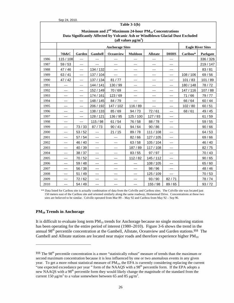
26

Sep 24, 2010. Table 3-1(b)

Maximum and 2nd Maximum 24-hour PM10 Concentrations Data Significantly Affected by Volcanic Ash or Windblown Glacial Dust Excluded

(all values μg/m3)

Anchorage Sites Eagle River Sites

7th&C Garden Gambell Oceanview Muldoon Allstate DHHS Caribou* Parkgate 1986 115 / 108 --- --- --- --- --- --- 336 / 3261987 59 / 53 --- --- --- --- --- --- 219 / 1471988 47 / 46 --- 134 / 132 --- --- --- --- 83 / 81 1989 63 / 41 --- 137 / 104 --- --- --- --- 108 / 106 69 / 56 1990 47 / 42 --- 137 / 134 81 / 77 --- --- --- 101 / 83 101 / 89 1991 --- --- 144 / 141 130 / 99 --- --- --- 180 / 148 78 / 72 1992 --- --- 152 / 149 70 / 69 --- --- --- 147 / 116 107 / 88 1993 --- --- 174 / 161 123 / 69 --- --- --- 71 / 66 79 / 77 1994 --- --- 148 / 145 84 / 79 --- --- --- 66 / 64 60 / 44 1995 --- --- 206 / 192 147 / 102 116 / 89 --- --- 102 / 80 60 / 51 1996 --- --- 138 / 133 85 / 69 94 / 73 72 / 61 --- 68 / 61 49 / 45 1997 --- --- 128 / 121 136 / 95 125 / 100 127 / 93 --- 61 / 59 1998 --- --- 115 / 98 61 / 54 76 / 58 88 / 78 --- 59 / 55 1999 --- 73 / 33 87 / 73 90 / 41 94 / 64 90 / 86 --- 90 / 66 2000 --- 53 / 52 --- 21 / 15 89 / 78 111 / 108 --- 64 / 53 2001 --- 57 / 54 --- --- 82 / 66 127 / 105 --- 69 / 66 2002 --- 46 / 40 --- --- 63 / 58 105 / 104 --- 46 / 40 2003 --- 40 / 39 --- --- 187 / 89 117 / 108 --- 82 / 75 2004 --- 38 / 37 --- --- 83 / 55 97 / 97 --- 70 / 43 2005 --- 70 / 52 --- --- 112 / 82 145 / 112 --- 90 / 65 2006 --- 59 / 48 --- --- --- 108 / 105 --- 65 / 60 2007 --- 56 / 38 --- --- --- 98 / 96 --- 48 / 46 2008 --- 51 / 49 --- --- --- 125 / 109 --- 70 / 53 2009 --- 72 / 62 --- --- --- 93 / 90 82 / 71 78 / 74 2010 --- 54 / 49 --- --- --- 155 / 98 89 / 65 93 / 72

** Data listed for Caribou site is actually combination of data from the Colville and Caribou sites. The Colville site was located just 150 meters east of the Caribou site and oriented similarly along the same roadway, Homestead Drive. Concentrations at these two sites are believed to be similar. Colville operated from Mar 89 – May 92 and Caribou from May 92 – Sep 96.

PM10 Trends in Anchorage It is difficult to evaluate long term PM10 trends for Anchorage because no single monitoring station has been operating for the entire period of interest (1980–2010). Figure 3-6 shows the trend in the annual 98th percentile concentration at the Gambell, Allstate, Oceanview and Garden stations.§§§ The Gambell and Allstate stations are located near major roads and therefore experience higher PM10

§§§ The 98th percentile concentration is a more “statistically robust” measure of trends than the maximum or second maximum concentration because it is less influenced by one or two anomalous events in any given year. To get a more robust statistical measure of PM10, the EPA is currently considering replacing the current “one expected exceedance per year ” form of the NAAQS with a 98th percentile form. If the EPA adopts a new NAAQS with a 98th percentile form they would likely change the magnitude of the standard from the current 150 μg/m3 to a value somewhere between 65 and 85 μg/m3.

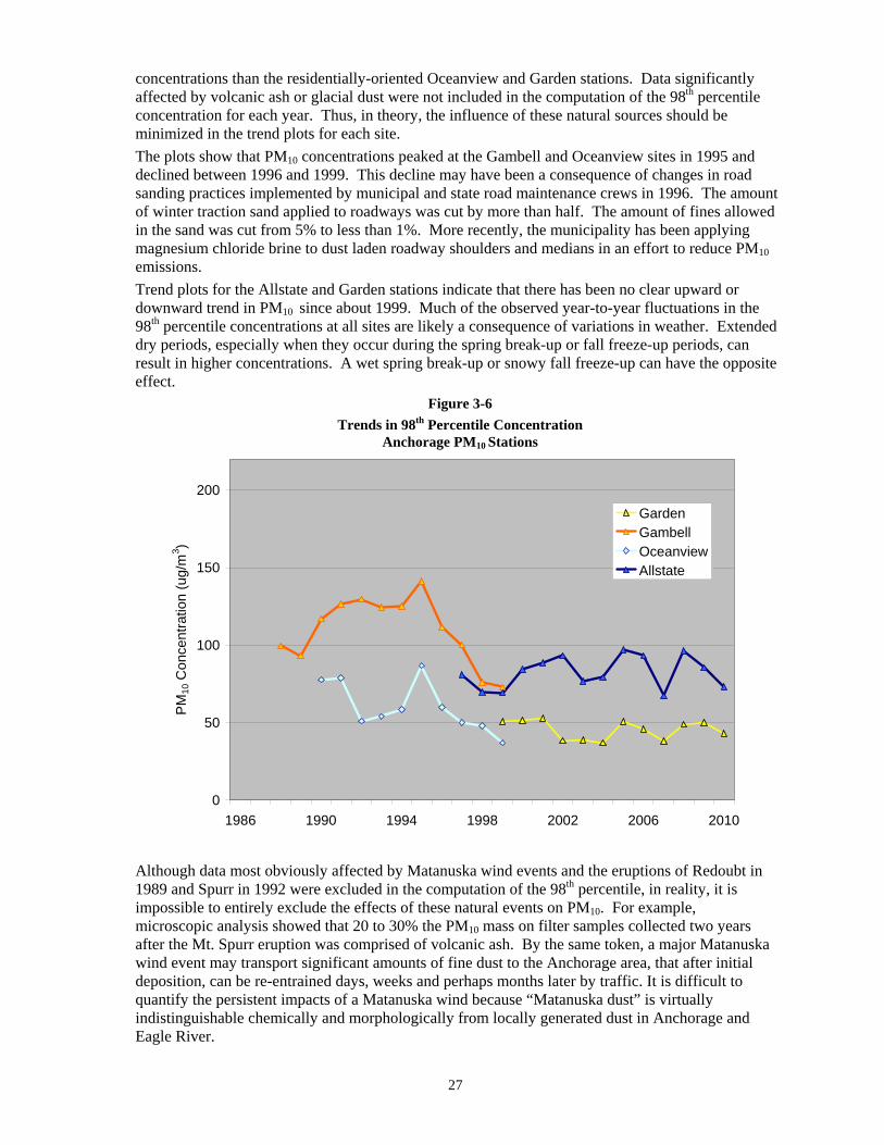
27

concentrations than the residentially-oriented Oceanview and Garden stations. Data significantly affected by volcanic ash or glacial dust were not included in the computation of the 98th percentile concentration for each year. Thus, in theory, the influence of these natural sources should be minimized in the trend plots for each site. The plots show that PM10 concentrations peaked at the Gambell and Oceanview sites in 1995 and declined between 1996 and 1999. This decline may have been a consequence of changes in road sanding practices implemented by municipal and state road maintenance crews in 1996. The amount of winter traction sand applied to roadways was cut by more than half. The amount of fines allowed in the sand was cut from 5% to less than 1%. More recently, the municipality has been applying magnesium chloride brine to dust laden roadway shoulders and medians in an effort to reduce PM10 emissions. Trend plots for the Allstate and Garden stations indicate that there has been no clear upward or downward trend in PM10 since about 1999. Much of the observed year-to-year fluctuations in the 98th percentile concentrations at all sites are likely a consequence of variations in weather. Extended dry periods, especially when they occur during the spring break-up or fall freeze-up periods, can result in higher concentrations. A wet spring break-up or snowy fall freeze-up can have the opposite effect.

Figure 3-6 Trends in 98th Percentile Concentration

Anchorage PM10 Stations

0

50

100

150

200

1986 1990 1994 1998 2002 2006 2010

PM

10 C

once

ntra

tion

(ug/

m3 )

GardenGambellOceanviewAllstate

Although data most obviously affected by Matanuska wind events and the eruptions of Redoubt in 1989 and Spurr in 1992 were excluded in the computation of the 98th percentile, in reality, it is impossible to entirely exclude the effects of these natural events on PM10. For example, microscopic analysis showed that 20 to 30% the PM10 mass on filter samples collected two years after the Mt. Spurr eruption was comprised of volcanic ash. By the same token, a major Matanuska wind event may transport significant amounts of fine dust to the Anchorage area, that after initial deposition, can be re-entrained days, weeks and perhaps months later by traffic. It is difficult to quantify the persistent impacts of a Matanuska wind because “Matanuska dust” is virtually indistinguishable chemically and morphologically from locally generated dust in Anchorage and Eagle River.

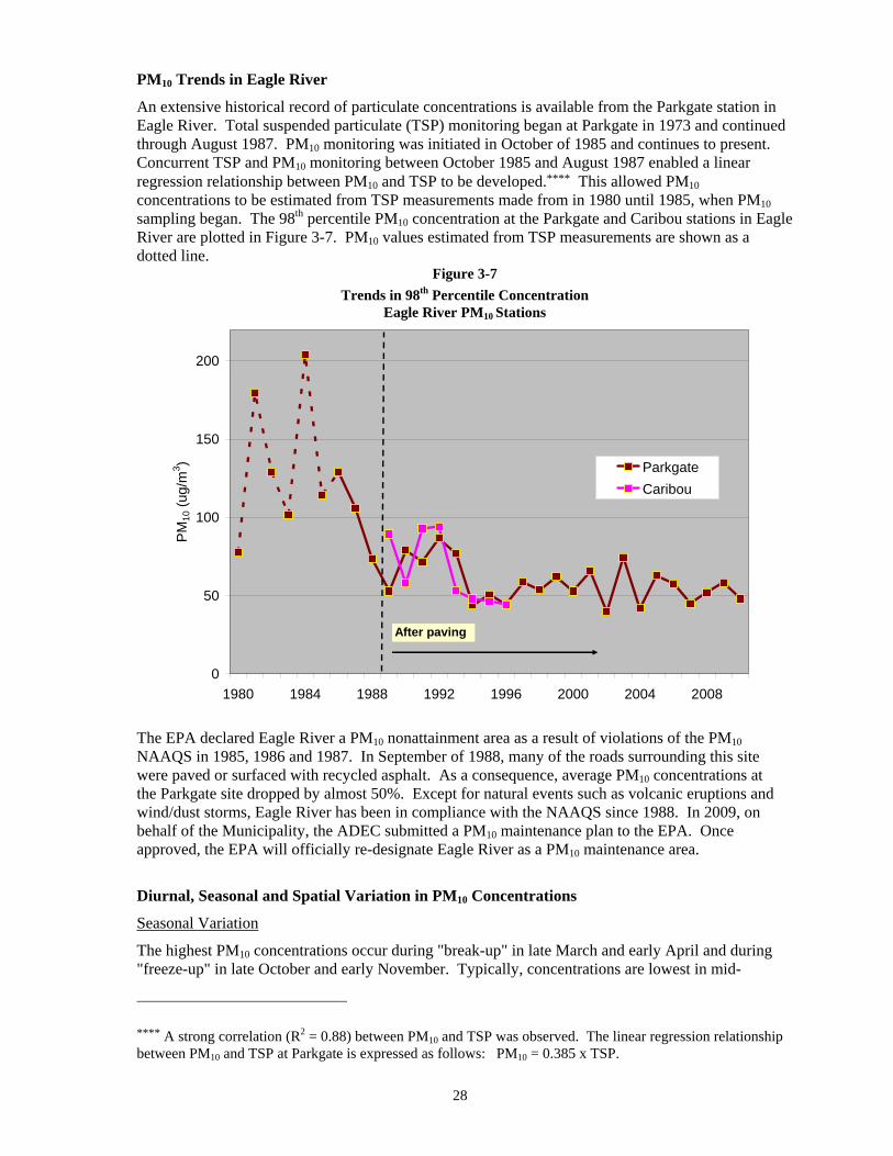
28

PM10 Trends in Eagle River

An extensive historical record of particulate concentrations is available from the Parkgate station in Eagle River. Total suspended particulate (TSP) monitoring began at Parkgate in 1973 and continued through August 1987. PM10 monitoring was initiated in October of 1985 and continues to present. Concurrent TSP and PM10 monitoring between October 1985 and August 1987 enabled a linear regression relationship between PM10 and TSP to be developed.**** This allowed PM10 concentrations to be estimated from TSP measurements made from in 1980 until 1985, when PM10 sampling began. The 98th percentile PM10 concentration at the Parkgate and Caribou stations in Eagle River are plotted in Figure 3-7. PM10 values estimated from TSP measurements are shown as a dotted line.

Figure 3-7 Trends in 98th Percentile Concentration

Eagle River PM10 Stations

0

50

100

150

200

1980 1984 1988 1992 1996 2000 2004 2008

PM

10 (u

g/m

3 ) ParkgateCaribou

After paving

The EPA declared Eagle River a PM10 nonattainment area as a result of violations of the PM10 NAAQS in 1985, 1986 and 1987. In September of 1988, many of the roads surrounding this site were paved or surfaced with recycled asphalt. As a consequence, average PM10 concentrations at the Parkgate site dropped by almost 50%. Except for natural events such as volcanic eruptions and wind/dust storms, Eagle River has been in compliance with the NAAQS since 1988. In 2009, on behalf of the Municipality, the ADEC submitted a PM10 maintenance plan to the EPA. Once approved, the EPA will officially re-designate Eagle River as a PM10 maintenance area.

Diurnal, Seasonal and Spatial Variation in PM10 Concentrations

Seasonal Variation

The highest PM10 concentrations occur during "break-up" in late March and early April and during "freeze-up" in late October and early November. Typically, concentrations are lowest in mid-

**** A strong correlation (R2 = 0.88) between PM10 and TSP was observed. The linear regression relationship between PM10 and TSP at Parkgate is expressed as follows: PM10 = 0.385 x TSP.

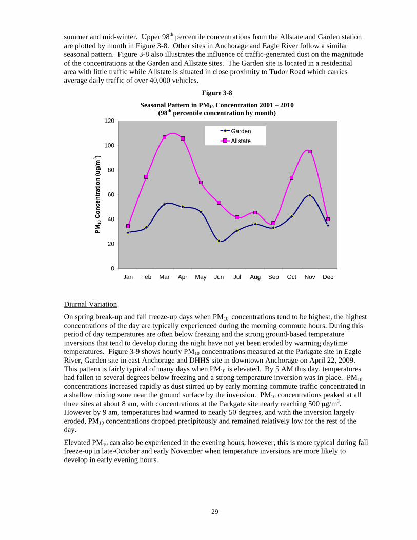
29

summer and mid-winter. Upper 98th percentile concentrations from the Allstate and Garden station are plotted by month in Figure 3-8. Other sites in Anchorage and Eagle River follow a similar seasonal pattern. Figure 3-8 also illustrates the influence of traffic-generated dust on the magnitude of the concentrations at the Garden and Allstate sites. The Garden site is located in a residential area with little traffic while Allstate is situated in close proximity to Tudor Road which carries average daily traffic of over 40,000 vehicles.

Figure 3-8

Seasonal Pattern in PM10 Concentration 2001 – 2010 (98th percentile concentration by month)

0

20

40

60

80

100

120

Jan Feb Mar Apr May Jun Jul Aug Sep Oct Nov Dec

PM10

Con

cent

ratio

n (u

g/m

3 )

GardenAllstate

Diurnal Variation

On spring break-up and fall freeze-up days when PM10 concentrations tend to be highest, the highest concentrations of the day are typically experienced during the morning commute hours. During this period of day temperatures are often below freezing and the strong ground-based temperature inversions that tend to develop during the night have not yet been eroded by warming daytime temperatures. Figure 3-9 shows hourly PM10 concentrations measured at the Parkgate site in Eagle River, Garden site in east Anchorage and DHHS site in downtown Anchorage on April 22, 2009. This pattern is fairly typical of many days when PM10 is elevated. By 5 AM this day, temperatures had fallen to several degrees below freezing and a strong temperature inversion was in place. PM10 concentrations increased rapidly as dust stirred up by early morning commute traffic concentrated in a shallow mixing zone near the ground surface by the inversion. PM10 concentrations peaked at all three sites at about 8 am, with concentrations at the Parkgate site nearly reaching 500 μg/m3. However by 9 am, temperatures had warmed to nearly 50 degrees, and with the inversion largely eroded, PM10 concentrations dropped precipitously and remained relatively low for the rest of the day.

Elevated PM10 can also be experienced in the evening hours, however, this is more typical during fall freeze-up in late-October and early November when temperature inversions are more likely to develop in early evening hours.

30

Figure 3-9

Hourly PM10 Concentrations on April 22, 2009 (Typical Diurnal PM10 Pattern during Spring Break-up Period)

0

50

100

150

200

250

300

350

400

450

500

12 AM 3 AM 6 AM 9 AM 12 PM 3 PM 6 PM 9 PM

PM10

Con

cent

ratio

n (u

g/m

3 )

ParkgateDHHSGarden

PM10 peak normally corresponds to the AM commute.

Spatial Variation

PM10 monitoring in Anchorage implicates major roadways as the source of PM10 emissions and the data suggest that except for natural events like volcanic eruptions and wind storms, PM10 exceedances occur only near major roadways. PM10 drops dramatically as the distance from the roadway increases. In 1997, during the spring break-up period, PM10 concentrations were measured at various setback distances from Gambell Street, a major traffic corridor in midtown Anchorage. Figure 3-10 shows that concentrations measured 160 meters from the road were about half those measured 15 meters back.

Figure 3-10

Average PM10 Concentration vs. Roadway Setback Gambell Street, Spring 1997

0

10

20

30

40

50

60

70

80

15 meters 40 meters 160 meters

Distance from Roadway

ug/m

3

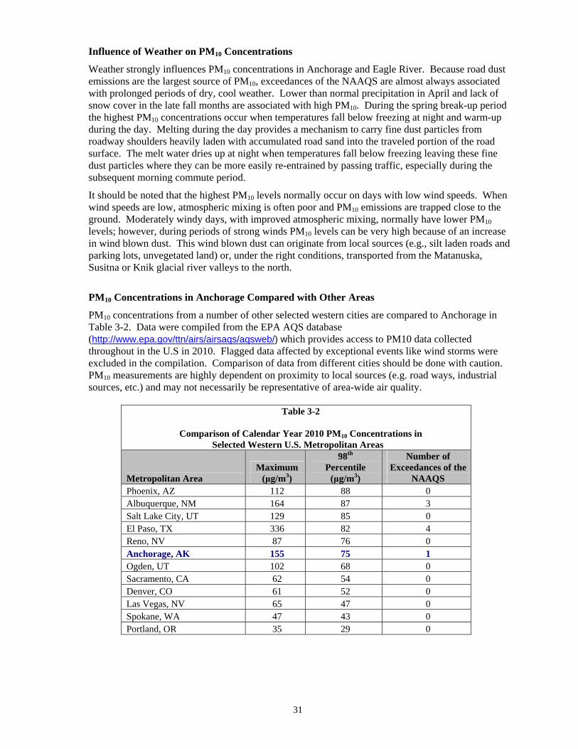
31

Influence of Weather on PM10 Concentrations

Weather strongly influences PM10 concentrations in Anchorage and Eagle River. Because road dust emissions are the largest source of PM10, exceedances of the NAAQS are almost always associated with prolonged periods of dry, cool weather. Lower than normal precipitation in April and lack of snow cover in the late fall months are associated with high PM10. During the spring break-up period the highest PM10 concentrations occur when temperatures fall below freezing at night and warm-up during the day. Melting during the day provides a mechanism to carry fine dust particles from roadway shoulders heavily laden with accumulated road sand into the traveled portion of the road surface. The melt water dries up at night when temperatures fall below freezing leaving these fine dust particles where they can be more easily re-entrained by passing traffic, especially during the subsequent morning commute period.

It should be noted that the highest PM10 levels normally occur on days with low wind speeds. When wind speeds are low, atmospheric mixing is often poor and PM10 emissions are trapped close to the ground. Moderately windy days, with improved atmospheric mixing, normally have lower PM10 levels; however, during periods of strong winds PM10 levels can be very high because of an increase in wind blown dust. This wind blown dust can originate from local sources (e.g., silt laden roads and parking lots, unvegetated land) or, under the right conditions, transported from the Matanuska, Susitna or Knik glacial river valleys to the north.

PM10 Concentrations in Anchorage Compared with Other Areas

PM10 concentrations from a number of other selected western cities are compared to Anchorage in Table 3-2. Data were compiled from the EPA AQS database (http://www.epa.gov/ttn/airs/airsaqs/aqsweb/) which provides access to PM10 data collected throughout in the U.S in 2010. Flagged data affected by exceptional events like wind storms were excluded in the compilation. Comparison of data from different cities should be done with caution. PM10 measurements are highly dependent on proximity to local sources (e.g. road ways, industrial sources, etc.) and may not necessarily be representative of area-wide air quality.

Table 3-2

Comparison of Calendar Year 2010 PM10 Concentrations in Selected Western U.S. Metropolitan Areas

Metropolitan Area Maximum

(μg/m3)

98th Percentile

(μg/m3)

Number of Exceedances of the

NAAQS Phoenix, AZ 112 88 0 Albuquerque, NM 164 87 3 Salt Lake City, UT 129 85 0 El Paso, TX 336 82 4 Reno, NV 87 76 0 Anchorage, AK 155 75 1 Ogden, UT 102 68 0 Sacramento, CA 62 54 0 Denver, CO 61 52 0 Las Vegas, NV 65 47 0 Spokane, WA 47 43 0 Portland, OR 35 29 0

32

PM2.5 Monitoring

The PM2.5 NAAQS was first adopted in 1997 and sampling with EPA-approved federal reference method (FRM) samplers began in Anchorage in November 1998. The PM2.5 FRM sampling is a filter-based method. Sample air is run through a pre-weighted 47 mm filter for 24 hours and the filter is re-weighed after the 24-hour collection period to determine the PM2.5 mass. The PM2.5 concentration is computed from this mass and the measured quantity of air that passed through the filter. These filter-based measurements were typically performed once every three days. In 2009 DHHS switched to continuous beta attenuation monitors (BAMs) that allow hourly PM2.5 measurements to be collected every day of the year. The 24-hour concentration is computed from these hourly measurements to assess compliance with the NAAQS. DHHS retained one FRM monitor at the Garden site to establish the correlation between the FRM and BAM measurement methods.††††

There are currently two BAM PM2.5 monitors operating in Anchorage and one in Eagle River, each providing hourly measurements of PM2.5. Monitoring was also conducted at a fourth location, the Allstate site near Tudor Road, between 1999 and 2002 using the filter-based FRM method.

Figure 3-11

PM2.5 Monitoring Network

Sources of PM2.5

Data collected thus far in Anchorage suggest that PM2.5 originates from different sources than PM10. While the majority of PM10 in Anchorage has been shown to be of geological origin such as pulverized winter traction sand, fine-grained soil particles, glacial silt and volcanic ash, the predominant sources of PM2.5 appear to be organic and elemental carbon from fireplace, woodstove

†††† A comparison of coincident BAM and FRM measurements suggests that while there is a good correlation between the

two measurement methods, the BAM consistently reports concentrations about 10% higher than the FRM.

33

and motor vehicle emissions. When particulate samples collected during the winter of 2009-2010 were subjected to carbon-14 analysis, fireplace and woodstoves accounted for about 70% of the carbon particulate on evenings and weekends, while motor vehicles accounted for about 60% of the carbon on weekday mornings.‡‡‡‡ Morning cold starts and warm-up idling are probably responsible for much of the motor vehicle contribution. Overall, the data point to wood stoves and fireplaces as the most significant sources of PM2.5, at least in residential areas. Motor vehicles exhaust emissions (both diesel and gasoline) may be a more important source near major roads and in commercial areas.

PM2.5 Data Summary

PM2.5 data from the three active and one discontinued monitor are summarized in Table 3-3. Annual average and 24-hour concentrations measured at all sites have been well below the NAAQS. The PM2.5 NAAQS is set at 15 µg/m3 as an annual average. The highest annual average recorded at Anchorage or Eagle River monitors was 7.2 µg/m3

, less than half the standard. The 24-hour average NAAQS is set at 35 µg/m3

for the 98th percentile value. No more than 2% of the days sampled may exceed this value, averaged over a three-year period.. Table 3-3 shows that all four monitoring sites have been well within the 24-hour and annual average NAAQS.

Table 3-3

Annual Average, Maximum and 98th Percentile PM2.5 Concentrations Garden Allstate Parkgate DHHS

Year Annual

Avg Annual

Max 98th %

AnnualAvg

AnnualMax

98th%

AnnualAvg

AnnualMax

98th %

Annual Avg

AnnualMax

98th

%

1999 6.4 69.8a 30.7 6.8 43.7 31.5 2000 5.4 27.2 12.2 6.1 32.8 20.2 2001 6.1 27.8 20.0 6.2 30.0 16.3 2002 6.0 16.9 15.8 6.9 20.8 18.2 2003 5.9 25.4 16.0 2004 7.0 43.7 31.9 2005 6.9 55.9b 17.9 2006 6.3 34.1 26.9 2007 4.9 17.6 14.0 2008 5.5 22.1 17.2 2009c 7.2 30.0 25.0 6.2 30.0 22.0 5.3 20.0 15.02010c 6.2 34.0 23.3 5.2 31.0 17.0 4.8 22.0 17.0a This value is considered suspect. Although no specific cause was identified that would allow this value to be flagged

or discounted, it is inconsistent with other data collected. b The 55.9 µg/m3 maximum was measured on July 15, 2005 and was the result of smoke from the Fox Creek fire near

Tustamena Lake on the Kenai Peninsula. c 2009 and 2010 data are from BAMs which report concentrations about 10% higher than the FRMs used prior.

‡‡‡‡ Carbon-14 analysis provides a way to date the age of the carbon found in the filter samples. “New” carbon is presumed to originate from wood burning, while “old” carbon is presumed to come from combusting fossil fuels like gasoline and diesel.

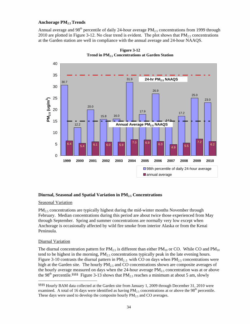
34

Anchorage PM2.5 Trends

Annual average and 98th percentile of daily 24-hour average PM2.5 concentrations from 1999 through 2010 are plotted in Figure 3-12. No clear trend is evident. The plot shows that PM2.5 concentrations at the Garden station are well in compliance with the annual average and 24-hour NAAQS.

Figure 3-12

Trend in PM2.5 Concentrations at Garden Station

30.7

12.2

20.0

15.8 16.0

31.9

17.9

26.9

17.2

25.023.0

14.0

6.45.4 6.1 6.0 5.9 6.2

7.25.54.9

6.36.97.0

0

5

10

15

20

25

30

35

40

1999 2000 2001 2002 2003 2004 2005 2006 2007 2008 2009 2010

PM2.

5 (ug

/m3 )

98th percentile of daily 24-hour averageannual average

24-hr PM2.5 NAAQS

Annual Average PM2.5 NAAQS

Diurnal, Seasonal and Spatial Variation in PM2.5 Concentrations

Seasonal Variation

PM2.5 concentrations are typically highest during the mid-winter months November through February. Median concentrations during this period are about twice those experienced from May through September. Spring and summer concentrations are normally very low except when Anchorage is occasionally affected by wild fire smoke from interior Alaska or from the Kenai Peninsula. Diurnal Variation

The diurnal concentration pattern for PM2.5 is different than either PM10 or CO. While CO and PM10 tend to be highest in the morning, PM2.5 concentrations typically peak in the late evening hours. Figure 3-10 contrasts the diurnal pattern in PM2..5 with CO on days when PM2.5 concentrations were high at the Garden site. The hourly PM2.5 and CO concentrations shown are composite averages of the hourly average measured on days when the 24-hour average PM2.5 concentration was at or above the 98th percentile.§§§§ Figure 3-13 shows that PM2.5 reaches a minimum at about 5 am, slowly §§§§ Hourly BAM data collected at the Garden site from January 1, 2009 through December 31, 2010 were examined. A total of 16 days were identified as having PM2.5 concentrations at or above the 98th percentile. These days were used to develop the composite hourly PM2.5 and CO averages.

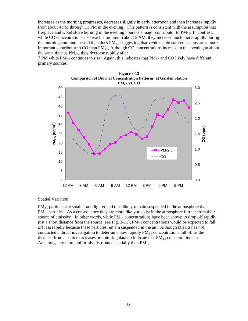
35

increases as the morning progresses, decreases slightly in early afternoon and then increases rapidly from about 4 PM through 11 PM in the evening. This pattern is consistent with the assumption that fireplace and wood stove burning in the evening hours is a major contributor to PM2.5. In contrast, while CO concentrations also reach a minimum about 5 AM, they increase much more rapidly during the morning commute period than does PM2.5 suggesting that vehicle cold start emissions are a more important contributor to CO than PM2.5. Although CO concentrations increase in the evening at about the same time as PM2.5, they decrease rapidly after 7 PM while PM2.5 continues to rise. Again, this indicates that PM2.5 and CO likely have different primary sources.

Figure 3-13 Comparison of Diurnal Concentration Patterns at Garden Station

PM2.5 vs. CO

0

5

10

15

20

25

30

35

40

45

50

12 AM 3 AM 6 AM 9 AM 12 PM 3 PM 6 PM 9 PM

PM2.

5 (ug

/m3 )

0.0

0.5

1.0

1.5

2.0

2.5

3.0

CO

(ppm

)

PM-2.5

CO

Spatial Variation

PM2.5 particles are smaller and lighter and thus likely remain suspended in the atmosphere than PM10 particles. As a consequence they are more likely to exist in the atmosphere further from their source of emission. In other words, while PM10 concentrations have been shown to drop off rapidly just a short distance from the source (see Fig. 3-11), PM2.5 concentrations would be expected to fall off less rapidly because these particles remain suspended in the air. Although DHHS has not conducted a direct investigation to determine how rapidly PM2.5 concentrations fall off as the distance from a source increases, monitoring data do indicate that PM2.5 concentrations in Anchorage are more uniformly distributed spatially than PM10.

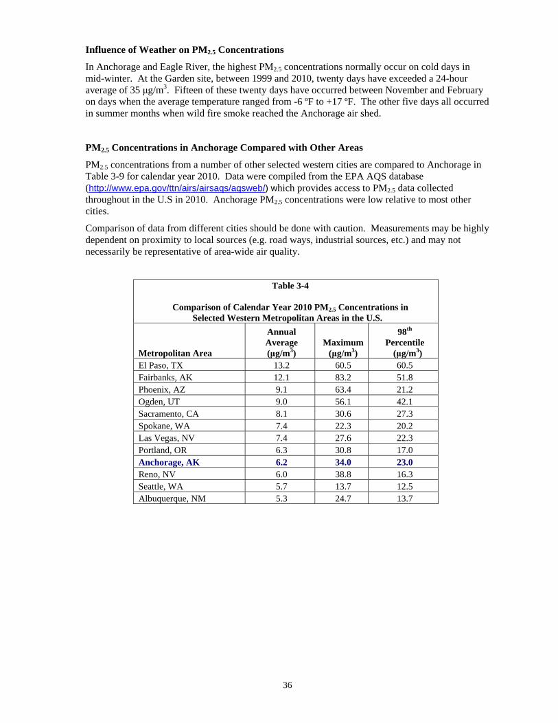
36

Influence of Weather on PM2.5 Concentrations

In Anchorage and Eagle River, the highest PM2.5 concentrations normally occur on cold days in mid-winter. At the Garden site, between 1999 and 2010, twenty days have exceeded a 24-hour average of 35 μg/m3. Fifteen of these twenty days have occurred between November and February on days when the average temperature ranged from -6 ºF to +17 ºF. The other five days all occurred in summer months when wild fire smoke reached the Anchorage air shed.

PM2.5 Concentrations in Anchorage Compared with Other Areas

PM2.5 concentrations from a number of other selected western cities are compared to Anchorage in Table 3-9 for calendar year 2010. Data were compiled from the EPA AQS database (http://www.epa.gov/ttn/airs/airsaqs/aqsweb/) which provides access to PM2.5 data collected throughout in the U.S in 2010. Anchorage PM2.5 concentrations were low relative to most other cities.

Comparison of data from different cities should be done with caution. Measurements may be highly dependent on proximity to local sources (e.g. road ways, industrial sources, etc.) and may not necessarily be representative of area-wide air quality.

Table 3-4

Comparison of Calendar Year 2010 PM2.5 Concentrations in Selected Western Metropolitan Areas in the U.S.

Metropolitan Area

Annual Average (μg/m3)

Maximum(μg/m3)

98th Percentile

(μg/m3) El Paso, TX 13.2 60.5 60.5 Fairbanks, AK 12.1 83.2 51.8 Phoenix, AZ 9.1 63.4 21.2 Ogden, UT 9.0 56.1 42.1 Sacramento, CA 8.1 30.6 27.3 Spokane, WA 7.4 22.3 20.2 Las Vegas, NV 7.4 27.6 22.3 Portland, OR 6.3 30.8 17.0 Anchorage, AK 6.2 34.0 23.0 Reno, NV 6.0 38.8 16.3 Seattle, WA 5.7 13.7 12.5 Albuquerque, NM 5.3 24.7 13.7

37

References 1. EPA AirData website, Office of Air and Radiation, U.S. Environmental Protection Agency.

http://www.epa.gov/air/data/.

2. “Particulate Air Pollution and Disease in Anchorage, Alaska,” Gordian M.E.; Ozkaynak,H.; Xue, J.; Morris, S.S.; Spengler, J.D. Environmental Health Perspectives, 104:290-297, March 1996

3. "Source of Particles on PM10 Filters, Anchorage, Alaska," Laboratory Report from Microlab Northwest for the Municipality of Anchorage, Report No. 1062-94, October 17, 1994

4. "Eagle River PM10 Control Plan," Municipality of Anchorage, Department of Health and Human Services, September 24, 1991

5. "Aerosol Characterization Study of Anchorage. Alaska: Chemical Analysis and Source Apportionment," prepared by NEA, Inc. for the Municipality of Anchorage, January 23, 1985

6. "Source Apportionment by Chemical Mass Balance Technique of PM10 Sources in Eagle River and Juneau, Alaska," prepared for the ADEC by NEA, Inc., May 23, 1988

7. “Identification, Quantification, and Control of PM10 Sources in Anchorage,” prepared by the Midwest Research Institute for the Municipality of Anchorage, April 15, 1999

8. Eagle River PM10 Limited Maintenance Plan,” proposed revision to the Alaska State Implementation Plan, adopted by the Anchorage Assembly, January 12, 2010.

9. “Contribution of wood-burning to wintertime particulate air pollution in Anchorage: Estimation by radiocarbon and polycyclic aromatic hydrocarbon analyses,” Municipality of Anchorage, Department of Health and Human Services, December 2010

38

Section 4 - Airborne Lead Health Effects of Lead

Exposure to airborne lead can occur directly by breathing or indirectly by eating lead-contaminated food, water, or non-food materials including dust and soil. The most common source of lead exposure is lead-contaminated dust from lead-based paint. Lead-based paint is common in older homes.

Fetuses, infants and children are most sensitive to lead exposure. Central nervous system damage can occur even at low exposures. There is an association between elevated blood lead levels and lower IQ test scores in children. Studies have implicated lead as a factor in high blood pressure and heart disease. Exposure to lead declined dramatically in the late 1980’s as a result of the reduction of lead in gasoline, paint, and the elimination of lead from soldered cans.*****

In October 2008, the EPA lowered the NAAQS for airborne lead ten-fold after reviewing new health and epidemiological data and concluding that health effects occur at much lower levels than previously believed. The NAAQS was lowered from 1.5 µg/m3 to 0.15 µg/m3

.

Sources of Lead in Anchorage

In the mid and early 1980's the main source of airborne lead in Anchorage was leaded gas. This source has been virtually eliminated as the result of federal regulation and voluntary efforts from local gasoline distributors. EPA reduced the allowable lead content in gasoline from an average of 1.0 grams per gallon to 0.1 grams per gallon by January 1, 1986. Nationwide, sales of leaded gasoline fell from about 40% of the retail market in 1984 to about 1% 1993. In Anchorage, none of the major gasoline retailers have offered leaded gasoline since 1993. Airborne Lead Monitoring in Anchorage

Airborne lead is sampled in much the same way as airborne particulate. A high volume sampler is used to draw large amounts of ambient air through a glass fiber filter. The filter is analyzed by atomic absorption spectrophotometry to determine the mass of lead collected in the filter. The concentration of lead in the air can be calculated if the volume of air and mass of lead in the sample are known.

Ambient concentrations of lead were measured at a five locations in Anchorage in the early and mid-1980's. Locations of the four lead sampling stations are described in Table 4-1. Lead monitoring was discontinued in 1987 when it became apparent that ambient lead levels in Anchorage had declined to levels well below the NAAQS as a result of the reduction of lead in gasoline.

Now that a new, more stringent lead NAAQS has been established, monitoring will again be performed in Anchorage to determine whether airborne levels are in compliance with the new standard. Monitoring is expected to begin in late 2011.

***** In the late 1970s the food industry began a gradual conversion from lead-soldered cans to welded cans. This conversion was completed by the industry in 1991, and FDA formally banned the sale of food packed in lead-soldered cans in 1996.

39

Table 4-1

Description of Airborne Lead Monitoring Stations in Anchorage

Site Name Monitoring Duration Location Gambell

October 1984 through December 1987 1950 Gambell Street

7th & C Street

March 1980 through March 1986 625 C Street at the old Anchorage Fire Department downtown station

8th & L Street

March 1980 through October 1982 Located near the northeast corner of 8th & L Street

Cheechako Street

Oct 1983 through March 1984 Located on Cheechako Street just south of Northern Lights Boulevard

Jefferson Avenue

Oct 1983 through March 1984 Located on Jefferson Avenue just west of Minnesota Drive

Summary of Anchorage Airborne Lead Data

Quarterly average airborne lead concentrations declined from above 1.0 μg/m3 in 1980 to less than 0.2 μg/m3 in 1987 when monitoring was terminated. In Anchorage, airborne lead concentrations were highest during the winter months. Lead data are summarized in Table 4-2.

Table 4-2

Quarterly Average Lead Concentrations at Anchorage Monitoring Stations Highest Quarterly Average Measured in Each Calendar Year

(all values in μg/m3)

Year 7th & C Street Gambell 8th & L Street Jefferson Avenu Cheechako Stree

1980 1.25* na 1.08* na na 1981 0.73 na 0.56 na na 1982 0.79 na 0.47* na na 1983 0.51 na na 1.41* 1.51* 1984 0.53 1.44* na 1.03* 1.43* 1985 0.22 0.56 na na na 1986 0.19* 0.36 na na na 1987 na 0.18 na na na

* Data from one or more quarters are missing

40

Airborne Lead Trends in Anchorage

The downward trend in the maximum quarterly lead concentration at the Gambell and 7th & C Street stations is illustrated in Figure 4-1. The NAAQS at the time this monitoring was conducted was set at 1.5 µg/m3. The new EPA standard is now set at 0.15 µg/m3.

Figure 4-1 Airborne Lead Trends at Two Anchorage Monitoring Stations

0.0

0.2

0.4

0.6

0.8

1.0

1.2

1.4

1.6

1980 1981 1982 1983 1984 1985 1986 1987

Lead

Con

cent

ratio

nug

/m3

7th and C Street Gambell

Lead Concentrations in Anchorage Compared with Other Areas In 1984, the maximum quarterly average lead concentration in Anchorage was higher than 95% or more of the 204 sites monitoring for lead in the U.S. At the current time, the status of Anchorage lead levels with respect to other cities is unknown. Because leaded fuel is still used in small aircraft, EPA has focused a portion of their initial nation-wide monitoring efforts on airports serving these planes. On EPA’s behalf, DHHS has agreed to monitor lead at Merrill Field Airport in east Anchorage beginning in late 2011. References 1. "National Air Quality and Emissions Trends Report, 1993," U.S. Environmental Protection

Agency, EPA 454/R-94-026, October 1994. 2. .”Fact Sheet – Final Revisions to the Ambient Air Quality Standards for Lead, EPA, October

2008. http://www.epa.gov/air/lead/pdfs/20081015pbfactsheet.pdf

41

Section 5 - Sulfur Dioxide Health Effects of Sulfur Dioxide

High concentrations of sulfur dioxide (SO2) may aggravate existing respiratory and cardiovascular disease. Asthmatics, and those with emphysema or bronchitis are the most sensitive to SO2 exposure. Children and the elderly may also be more sensitive. SO2 also contributes to acid rain. Acid rain can lead to the acidification of lakes and streams, damage trees, and erode historic building and statues, especially those constructed from limestone or marble.

In 2010 the EPA set a new one-hour standard for SO2 at 75 ppb.††††† The new standard was established on the basis of new scientific evidence linking short term exposure to SO2 to respiratory illness and increases in hospital visits. They also retained the previously established limits for a 3-hour average (500 ppb), 24-hour average (140 ppb) and annual average (30 ppb) until EPA determines whether areas meet the new standard.

Sources of SO2 in Anchorage

There are no significant sources of SO2 in Anchorage. SO2 is emitted primarily from stationary source coal and oil combustion, steel mills, refineries, pulp and paper mills, and from non-ferrous smelters. These activities are very limited or non-existent in Anchorage. Natural gas is used almost exclusively to fuel electrical power generating facilities in the Anchorage area.

SO2 Monitoring in Anchorage

SO2 was monitored in Anchorage from April 1983 through December 1984 at a site in downtown Anchorage. The levels of SO2 measured were uniformly low and well below the NAAQS. More recently, between March 1999 and June 2000, the ADEC Data collected “unofficial data” from a site near the Chugach Electric Power Generation Plant at International Airport Road. Because these data were collected as part of staff training exercise they were never certified or subjected to quality assurance procedures normally applied. However, with this caveat in mind, the data suggest that SO2 concentrations in Anchorage were likely well below all applicable standards. The annual average concentration measured in Anchorage during the one-year period April 1, 1999 - March 31, 2000 was 1 ppb, about 30 times below the NAAQS. The one-hour average and three-hour average were also very low, an order of magnitude lower than applicable standards.

SO2 Concentrations in Anchorage Compared with Other Areas

Unofficial data collected from the Chugach Electric Power Generation Plant at International Airport Road during the one-year period April 1, 1999 – March 31, 2000 were compared to summary data on the EPA AQS database for calendar year 1999. Comparison suggests that if the Anchorage data were included in the database, one-hour, three-hour and annual average concentrations would have been in the lowest (bottom 1%) of the 641 monitors reporting nationwide .

References

1. "National Air Quality and Emissions Trends Report, 1993," U.S. Environmental Protection Agency, EPA 454/R-94-026, October 1994.

2. EPA AirData website, Office of Air and Radiation, U.S. Environmental Protection Agency. http://www.epa.gov/air/data/

††††† To attain this standard, the 3-year average of the 99th percentile of the daily maximum 1-hour average may not exceed 75 ppb.

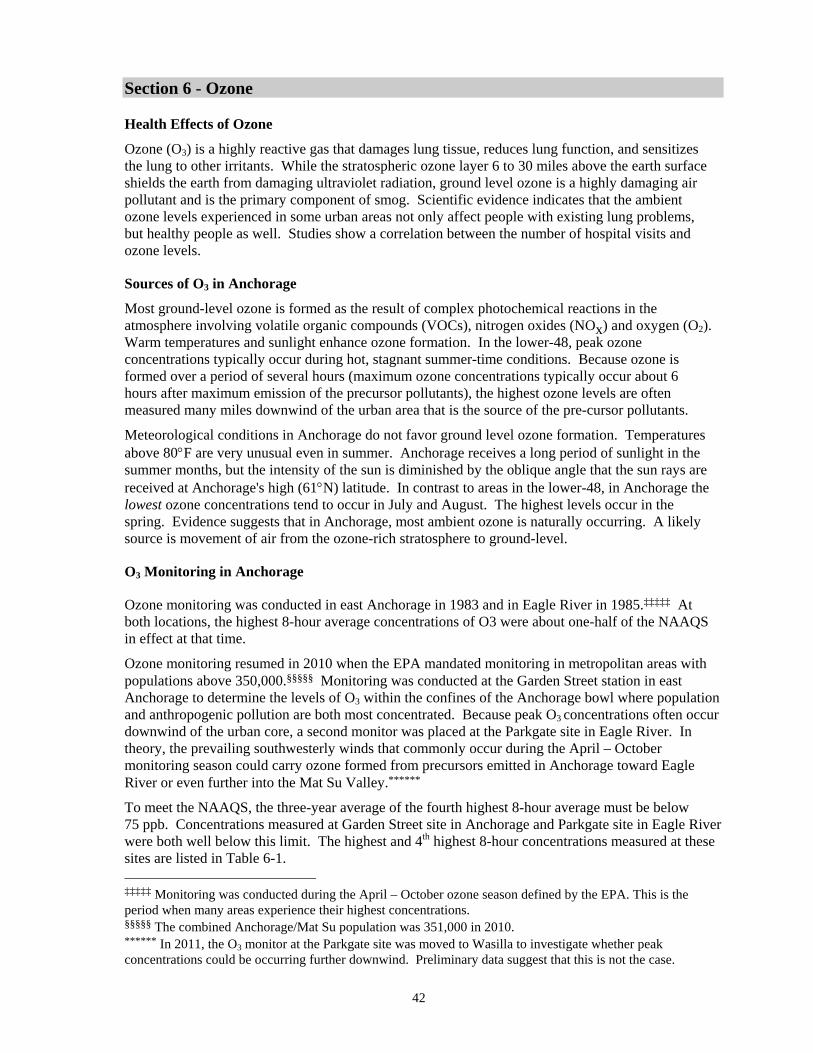
42

Section 6 - Ozone Health Effects of Ozone

Ozone (O3) is a highly reactive gas that damages lung tissue, reduces lung function, and sensitizes the lung to other irritants. While the stratospheric ozone layer 6 to 30 miles above the earth surface shields the earth from damaging ultraviolet radiation, ground level ozone is a highly damaging air pollutant and is the primary component of smog. Scientific evidence indicates that the ambient ozone levels experienced in some urban areas not only affect people with existing lung problems, but healthy people as well. Studies show a correlation between the number of hospital visits and ozone levels.

Sources of O3 in Anchorage

Most ground-level ozone is formed as the result of complex photochemical reactions in the atmosphere involving volatile organic compounds (VOCs), nitrogen oxides (NOx) and oxygen (O2). Warm temperatures and sunlight enhance ozone formation. In the lower-48, peak ozone concentrations typically occur during hot, stagnant summer-time conditions. Because ozone is formed over a period of several hours (maximum ozone concentrations typically occur about 6 hours after maximum emission of the precursor pollutants), the highest ozone levels are often measured many miles downwind of the urban area that is the source of the pre-cursor pollutants.

Meteorological conditions in Anchorage do not favor ground level ozone formation. Temperatures above 80°F are very unusual even in summer. Anchorage receives a long period of sunlight in the summer months, but the intensity of the sun is diminished by the oblique angle that the sun rays are received at Anchorage's high (61°N) latitude. In contrast to areas in the lower-48, in Anchorage the lowest ozone concentrations tend to occur in July and August. The highest levels occur in the spring. Evidence suggests that in Anchorage, most ambient ozone is naturally occurring. A likely source is movement of air from the ozone-rich stratosphere to ground-level.

O3 Monitoring in Anchorage

Ozone monitoring was conducted in east Anchorage in 1983 and in Eagle River in 1985.‡‡‡‡‡ At both locations, the highest 8-hour average concentrations of O3 were about one-half of the NAAQS in effect at that time.

Ozone monitoring resumed in 2010 when the EPA mandated monitoring in metropolitan areas with populations above 350,000.§§§§§ Monitoring was conducted at the Garden Street station in east Anchorage to determine the levels of O3 within the confines of the Anchorage bowl where population and anthropogenic pollution are both most concentrated. Because peak O3 concentrations often occur downwind of the urban core, a second monitor was placed at the Parkgate site in Eagle River. In theory, the prevailing southwesterly winds that commonly occur during the April – October monitoring season could carry ozone formed from precursors emitted in Anchorage toward Eagle River or even further into the Mat Su Valley.******

To meet the NAAQS, the three-year average of the fourth highest 8-hour average must be below 75 ppb. Concentrations measured at Garden Street site in Anchorage and Parkgate site in Eagle River were both well below this limit. The highest and 4th highest 8-hour concentrations measured at these sites are listed in Table 6-1. ‡‡‡‡‡ Monitoring was conducted during the April – October ozone season defined by the EPA. This is the period when many areas experience their highest concentrations. §§§§§ The combined Anchorage/Mat Su population was 351,000 in 2010. ****** In 2011, the O3 monitor at the Parkgate site was moved to Wasilla to investigate whether peak concentrations could be occurring further downwind. Preliminary data suggest that this is not the case.

43

Table 6-1

Highest and 4th Highest Ozone Concentrations April 1, 2010 – October 31, 2010

Site

Maximum 8-hr Average

(ppb)

4th highest 8-hr Average

(ppb)

Garden Street (east Anchorage) 47.1 43.8

Parkgate (Eagle River) 50.4 47.3

O3 Concentrations in Anchorage Compared with Other Areas Ozone concentrations in Anchorage and Eagle River are low compared to the rest of the U.S. Data from Anchorage and Eagle River in 2010 were compared with summary data from the 1,293 sites nationwide that reported their data to the EPA AQS database in 2009. Summary data from 2010 are not available as this report is being written. The maximum and 4th maximum 8-hour averages measured in Anchorage and Eagle River in 2010 were lower than 99% of sites nationwide in 2009.

Interestingly, the ozone levels measured at the Garden Street in Anchorage and Parkgate in Eagle River between April and October 2010 were 5 to 10% lower, on average, than those found in Denali National Park. Peak concentrations were also lower. It is speculated that natural background levels of ozone are similar at all three sites, but some of this natural ozone is being removed through chemical reactions (called scavenging) with urban pollutants in Anchorage and Eagle River. This may also explain why ozone concentrations are slightly higher in Eagle River than in the Anchorage bowl. Scavenging is likely more of a factor around the more urbanized (and polluted) Garden Street site in the Anchorage bowl than at the Parkgate site in Eagle River. References 1. EPA AirData website, Office of Air and Radiation, U.S. Environmental Protection Agency.

http://www.epa.gov/air/data/

44

Section 7 - Nitrogen Dioxide Health Effects of Nitrogen Dioxide

Nitrogen dioxide (NO2) is a brownish, highly reactive gas that can irritate the lungs, cause bronchitis and pneumonia, and lower resistance to respiratory infections. Continued and repeated exposure to high concentrations of NO2 may cause acute respiratory disease in children.

NO2 is an important precursor in the formation of ozone or smog. Consequently, control of NO2 emissions is an important component of overall pollution reduction strategies in areas with ozone problems. NO2 is also a precursor in the formation nitric acid and other acid aerosols that may affect aquatic and terrestrial ecosystems.

In 2010 the EPA set a new one-hour standard for NO2 at 100 ppb.†††††† The new standard was established on the basis of new scientific evidence linking short term exposure to NO2 to respiratory illness and increases in hospital visits. They also retained the previously established long-term, annual average limit of 53 ppb.

Sources of NO2 in Anchorage

Nationwide, the main sources of NO2 are industrial fuel combustion, electrical power generation and air and land transportation. In Anchorage, a comprehensive NO2 inventory has not been prepared. However, the main sources of NO2 in Anchorage are probably similar to the U.S. as a whole. Motor vehicles, natural gas combustion for electrical power, and aircraft are likely the major sources of NO2 in Anchorage.

NO2 Monitoring in Anchorage

The only NO2 monitoring data available for Anchorage was collected by the ADEC between March 1999 and June 2000. “Unofficial data” were collected near the Chugach Electric Power Generation Plant at International Airport Road as part of a staff training exercise. These data were never certified or subjected to quality control procedures normally applied to air quality data. Although caution should be exercised when interpreting analyses of data of unknown quality, the annual average concentration was 17 ppb, well below the 53 ppb NAAQS. The 98th percentile hourly concentration was 55 ppb which is also well below the new hourly NAAQS of 100 ppb.

NO2 Concentrations in Anchorage Compared with Other Areas

The unofficial data collected from the Chugach Electric Power Generation Plant at International Airport Road during the one-year period April 1, 1999 – March 31, 2000 were compared to summary data on the EPA AQS database for calendar year 1999. Comparison suggests that if Anchorage were included in the database it would have ranked about in the middle (50th percentile) of the 436 monitors reporting nationwide.

References

1. EPA AirData website, Office of Air and Radiation, U.S. Environmental Protection Agency. http://www.epa.gov/air/data/

†††††† The 98th percentile of hourly concentrations, averaged over a 3-year period must be below 100 ppb to be considered in attainment with the NAAQS.

45

Section 8 – Toxic Air Pollutants

Health Effects of Toxic Air Pollutants

Toxic air pollutants, also known as hazardous air pollutants (HAPs), are those pollutants that are known or suspected to cause cancer or other serious health effects, such as reproductive effects or birth defects, or adverse environmental effects. EPA has designated 188 specific pollutants as hazardous air pollutants. They include carbon-based volatile organic compounds (VOCs) such as benzene and toluene which are found in gasoline; perchloroethylene, which is emitted from some dry cleaning facilities; and methylene chloride, which is used as a solvent and paint stripper by a number of industries. Examples of other listed air toxics include asbestos and metals such as cadmium, mercury, and chromium. Unlike the criteria pollutants discussed earlier in this report, EPA has not established ambient air quality standards for HAPs.

The criteria pollutants (CO, PM, SO2, O3 and NO2) are not included among the 188 HAPs. However airborne lead is considered to be both a criteria pollutant and a HAP.

Much of the monitoring conducted in Anchorage has focused on HAPs associated with motor vehicle exhaust or evaporative emissions . Benzene has been of particular interest. Long-term exposure to high levels of benzene in air has been shown to cause leukemia. Leukemia and lymphomas and other tumor types have been observed in experimental animals exposed to benzene by inhalation or oral administration. A number of adverse non-cancer effects have been associated with exposures to high levels (>50,000 ppb) for long periods of time. Studies addressing the risk of leukemia at moderate or low levels of exposure have been inconclusive. Some studies have found that mortality rates for leukemia among workers potentially exposed to petroleum products (and presumably benzene) are not higher than the general population. However, a recent study has shown higher levels of nonlymphotic leukemia in truck drivers, gas station attendants and those employed in jobs with greater exposure to petroleum products.

Ambient benzene exposures are substantially lower than the occupational exposures in the studies above. In the U.S., benzene concentrations in outdoor or ambient air rarely exceed 10 ppb even in the most polluted urban areas. Ambient concentrations of benzene are generally an order of magnitude or greater below the levels found in occupational settings involving contact with petroleum products.

Limited monitoring has also been performed for 1,3-butadiene, acetaldehyde and formaldehyde, and for polycyclic aromatic hydrocarbons (PAHs) such as naphthalene. All are recognized carcinogens. Animal studies indicate that high concentrations of 1, 3-butadiene, formaldehyde, and acetaldehyde cause cancer in animals exposed through inhalation. Human epidemiological studies on these compounds are limited. Epidemiological evidence has implicated formaldehyde with increases in nasopharyngeal, nasal cavity and sinus cancers.

Air Toxics Monitoring in Anchorage

Over the past twenty years, DHHS has conducted four ambient (outdoor) air toxics monitoring studies and a number of indoor studies. All have focused at least in part on benzene. In general, these studies suggest that concentrations of gasoline-related VOCs such as benzene, ethyl benzene, toluene and xylene (BETX) are higher in Anchorage than most communities in the U.S. Concentrations are highest in the winter months and are strongly correlated with CO concentrations. Motor vehicle exhaust emissions have been shown to be the main source of CO emissions in Anchorage and they are likely the main source of ambient BETX as well.

The four ambient studies conducted in Anchorage are briefly summarized below, starting with the most recent study which is still in progress.

46

Assessment of the Effectiveness of Gasoline Benzene Content Reductions on Ambient Benzene Concentrations (2008-09)

In 2009 DHHS completed the first phase of a two phase study that is examining the effect of new EPA-mandated reductions in the benzene content of gasoline on ambient benzene concentrations in Anchorage. The new EPA gasoline rules are expected to reduce the benzene content of gasoline in Anchorage from about 5% to 1.3% or less by 2012.

Phase 1 of this study provided a one-year “snapshot” of ambient benzene levels before the new EPA gasoline rules take effect. Phase 2, which is planned to begin sometime in late 2012 after the rule takes effect, will take another one-year snapshot to determine how effective it has been in lowering the levels of benzene in ambient air.

In Phase 1, ambient concentrations of benzene, other VOCs and PAHs were measured at the Garden station in east Anchorage over a one-year period ending October 2009. One 24-hour Summa air canister sample was collected every six days and sent to the EPA national contract laboratory for analysis of benzene and thirty other VOCs. During this same period, gasoline samples were collected from twenty Anchorage gas stations to measure the content of benzene and other VOCs. The average benzene content of the gasoline sampled was 5% and varied very little over the course of the year. The level of benzene in Anchorage gasoline was two to ten times higher than levels typically found in the “lower-48.”

The average ambient benzene concentration measured during Phase 1 was 1.1 ppb. The highest benzene concentrations were observed in the winter and were highly correlated (R2 = 0.93) with ambient CO. Figure 8-1 shows a plot of 24-hour average concentrations of benzene and CO measured during Phase 1.

Figure 8-1

Ambient Benzene and CO Concentration at Garden Site Oct 22, 2008 – Oct 16, 2009

0

1

2

3

4

5

6

7

8

Oct Dec Feb Apr Jun Aug Oct

benz

ene

(ppb

)

0.0

0.5

1.0

1.5

2.0

2.5

3.0

CO

(ppm

)

benzeneCO

The ambient concentrations of benzene and other VOCs and PAHs measured during Phase 1 were compared with data collected in other cities around the U.S. in calendar year 2008.‡‡‡‡‡‡ Among monitoring sites nation-wide, Anchorage ranked in the 98th percentile or higher for benzene, ethyl benzene, toluene and o-xylene. BETX concentrations measured at the Garden site were similar to

‡‡‡‡‡‡ Slightly different time periods were compared. CY 2008 data from the AIRS AQS database http://www.epa.gov/air/data/ were compared to Phase 1 data collected Oct 2008 – Oct 2009.

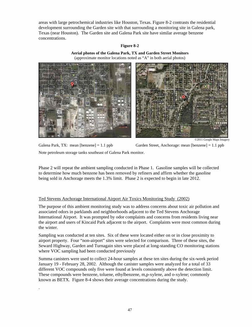
47

areas with large petrochemical industries like Houston, Texas. Figure 8-2 contrasts the residential development surrounding the Garden site with that surrounding a monitoring site in Galena park, Texas (near Houston). The Garden site and Galena Park site have similar average benzene concentrations.

Figure 8-2

Aerial photos of the Galena Park, TX and Garden Street Monitors (approximate monitor locations noted as “A” in both aerial photos)

©2011 Google Maps Imagery

Galena Park, TX: mean [benzene] = 1.1 ppb Garden Street, Anchorage: mean [benzene] = 1.1 ppb

Note petroleum storage tanks southeast of Galena Park monitor.

Phase 2 will repeat the ambient sampling conducted in Phase 1. Gasoline samples will be collected to determine how much benzene has been removed by refiners and affirm whether the gasoline being sold in Anchorage meets the 1.3% limit. Phase 2 is expected to begin in late 2012.

Ted Stevens Anchorage International Airport Air Toxics Monitoring Study (2002)

The purpose of this ambient monitoring study was to address concerns about toxic air pollution and associated odors in parklands and neighborhoods adjacent to the Ted Stevens Anchorage International Airport. It was prompted by odor complaints and concerns from residents living near the airport and users of Kincaid Park adjacent to the airport. Complaints were most common during the winter.

Sampling was conducted at ten sites. Six of these were located either on or in close proximity to airport property. Four “non-airport” sites were selected for comparison. Three of these sites, the Seward Highway, Garden and Turnagain sites were placed at long-standing CO monitoring stations where VOC sampling had been conducted previously

Summa canisters were used to collect 24-hour samples at these ten sites during the six-week period January 19 - February 28, 2002. Although the canister samples were analyzed for a total of 33 different VOC compounds only five were found at levels consistently above the detection limit. These compounds were benzene, toluene, ethylbenzene, m,p-xylene, and o-xylene; commonly known as BETX. Figure 8-4 shows their average concentrations during the study.

.

48

Figure 8-3

Average Concentration of BETX Compounds at Canister Sampling Sites Ted Stevens Anchorage International Airport Air Toxics Monitoring Study

January 19 – February 28, 2002

0

1

2

3

4

5

6

7

8

Kincaid LittleCampbell

Lake

NorthRunway

NationalWeatherService

JonesLake

BConcourse

OceanDockRoad

Turnagain Garden SewardHighway

Con

cent

ratio

n(p

pbv)

Benzene

Toluene

m,p-Xylene

Ethylbenzene

o-Xylene

"non airport" sites

airport sites

Figure 8-3 shows that BETX concentrations at the six sites nearest the airport were lower than the four “non-airport” sites. Canister sites located in areas with the most motor vehicle activity had the highest BETX concentrations and these sites were located away from the airport. The highest average BETX concentration was measured at the Seward Highway site, located at the busiest intersection in Anchorage. The two lowest concentration sites, at Kincaid Park and Little Campbell Lake were a significant distance from roadways and parking lots.

The data from this study were examined to determine whether any of the VOCs tested might be specifically associated with diesel and/or aircraft exhaust. No associations were found. This suggests that the compounds causing odors were not among the compounds analyzed or that the compounds creating odors are present at levels below the reporting limit of the analytical method employed in this study. Of the 33 compounds tested, 28 were consistently below their reporting limit.

Indoor and Outdoor VOC Assessment (1994-96)

The purpose of this air quality monitoring study was to measure and assess indoor and outdoor concentrations of VOCs during the period when ethanol-blended gasoline was being used in Anchorage. This study was conceived to help address concerns about possible health impacts of using ethanol-blended gasoline in a sub-arctic climate and to gather baseline information on indoor VOC exposures and sources within the home.

Ambient VOC monitoring was performed at existing sites (Garden, Spenard & Benson, and Sand Lake) where CO was being monitored to investigate the relationship between VOC concentrations

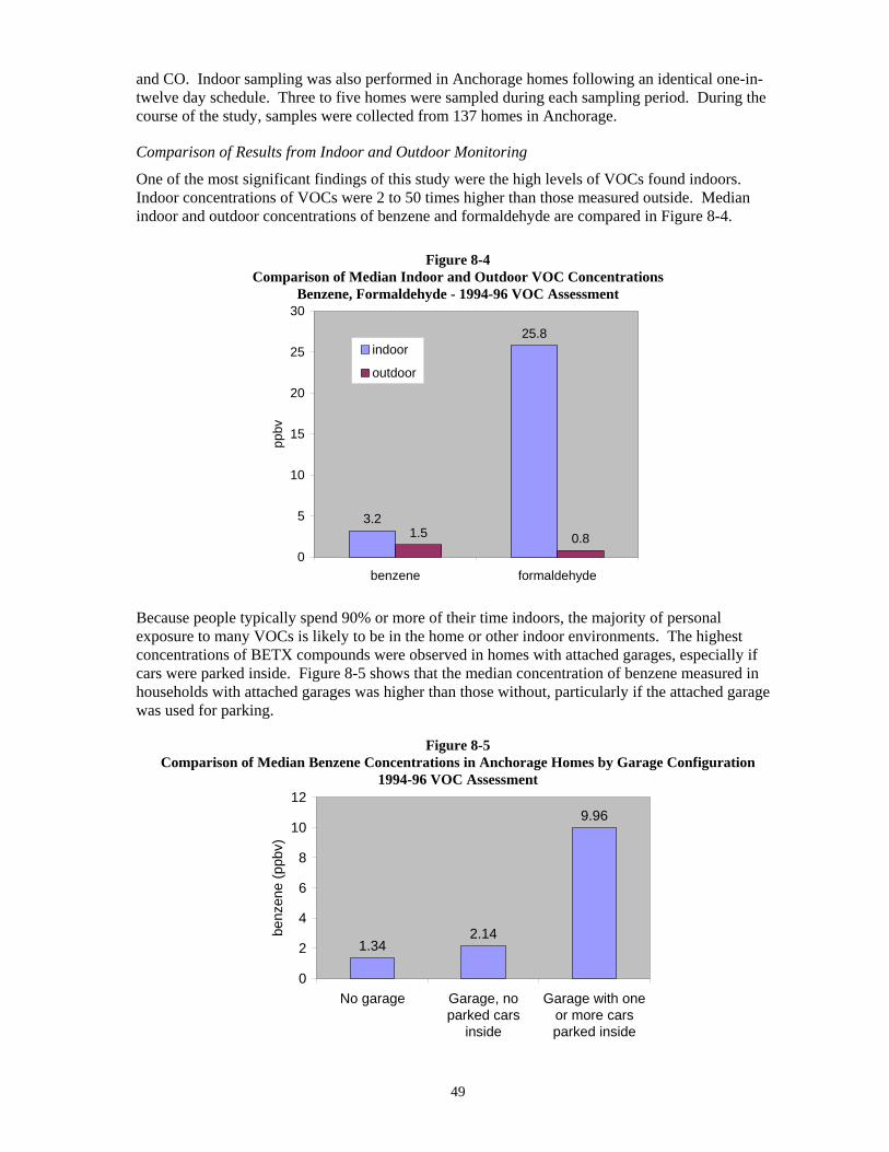
49

and CO. Indoor sampling was also performed in Anchorage homes following an identical one-in-twelve day schedule. Three to five homes were sampled during each sampling period. During the course of the study, samples were collected from 137 homes in Anchorage.

Comparison of Results from Indoor and Outdoor Monitoring

One of the most significant findings of this study were the high levels of VOCs found indoors. Indoor concentrations of VOCs were 2 to 50 times higher than those measured outside. Median indoor and outdoor concentrations of benzene and formaldehyde are compared in Figure 8-4.

Figure 8-4

Comparison of Median Indoor and Outdoor VOC Concentrations Benzene, Formaldehyde - 1994-96 VOC Assessment

3.2

25.8

1.5 0.80

5

10

15

20

25

30

benzene formaldehyde

ppbv

indoor

outdoor

Because people typically spend 90% or more of their time indoors, the majority of personal exposure to many VOCs is likely to be in the home or other indoor environments. The highest concentrations of BETX compounds were observed in homes with attached garages, especially if cars were parked inside. Figure 8-5 shows that the median concentration of benzene measured in households with attached garages was higher than those without, particularly if the attached garage was used for parking.

Figure 8-5

Comparison of Median Benzene Concentrations in Anchorage Homes by Garage Configuration 1994-96 VOC Assessment

1.342.14

9.96

0

2

4

6

8

10

12

No garage Garage, noparked cars

inside

Garage with oneor more carsparked inside

benz

ene

(ppb

v)

50

The data indicated that motor vehicle and/or gasoline-related emissions were not a significant source of indoor formaldehyde or acetaldehyde, however. These compounds were not correlated with the indoor BETX measurements indicating that they have a different source than the BETX compounds.

Government Hill VOC Monitoring Study (1993-94)

The primary purpose of this study was to address concerns about VOC exposures among residents of the Anchorage’s Government Hill neighborhood just north of downtown. Government Hill was bounded on the west and east by fuel storage facilities (tank farms) and these facilities created fuel odors that were the source of frequent complaints and concern by nearby residents.

VOC sampling was conducted at three sites in Government Hill and at eight other locations in Anchorage for comparison. The locations of the sites are shown in Figure 8-6.

Figure 8-6 Anchorage VOC Monitoring Study (1993-94) Sampling Locations

1 Downtown, 6th and E Street 2 Government Hill bluff, Delaney St. & W. Cook 3 Government Hill, Cunningham St. & E. Manor 4 Government Hill Elementary School 5 Benson CO station, Spenard Rd. & Benson Blvd 6 Airport Post Office, Postmark Drive 7 Raspberry Road near Tanaina Drive 8 Sand Lake CO station, Raspberry near Jewel Lake Rd. 9 Lower Hillside area 10 Garden CO station, 16th & Garden St. 11 Muldoon area

51

A 24-hour sample was collected every 12 days during the 14 month study for 37 possible VOCs. Quantifiable levels of seven VOCs were regularly observed in the samples. Benzene, toluene, ethyl benzene, m & p-xylene, o-xylene, and 1,3,5 & 1,2,4 trimethylbenzene were all found in reportable quantities. Because of its known carcinogenicity, benzene was of the greatest interest. Benzene data are summarized in Table 8-1.

Table 8-1

Government Hill VOC Monitoring Study Mean, Maximum, and Minimum Benzene Concentrations

April 1993 – April 1994

Site

Location

Mean Concentration

(ppb)

Max Concentration

(ppb)

Min Concentration

(ppb) 1 Downtown 2.5 8.8 0.4 2 Gov Hill (bluff) 3.7 8.7 0.6 3 Gov Hill (Delaney St.) 2.3 7.0 1.0 4 Gov Hill School 1.8 7.8 0.4 5 Benson / Spenard Blvd. 5.4 20.8 1.0 6 Airport Post Office 2.0 7.0 0.3 7 Tanaina Drive 1.2 3.3 0.2 8 Sand Lake 2.4 10.4 0.4 9 Lower Hillside 1.4 3.7 0.3 10 16th and Garden St 3.6 14.0 0.5 11 Muldoon 2.2 11.0 0.4

The highest concentrations of benzene were found in central Anchorage at Site #5 near the intersection of Spenard Road and Benson Boulevard. The second highest concentration was found at Site #2 in Government Hill located on a bluff above and less than 50 meters from a gasoline bulk storage tank.

Data suggested that motor vehicles were the primary source of benzene and other VOCs in most of Anchorage. A very strong association was observed between CO concentrations and VOCs.

In Government Hill, evaporative emissions from the tank farm appeared to be a significant source of ambient benzene and other VOCs. The highest benzene and VOC concentrations were found at the bluff site closest to the tanks. At the other two Government Hill sites, located further away from the tanks, motor vehicle emissions appeared to be the source of the majority of the ambient benzene but evaporative emissions from the tanks was still a contributor. Overall, ambient benzene exposures at these two sites were typical of other Anchorage residential areas even with the added contribution from the tank farm.

Ambient Air Toxics Trends

Determining air toxics trends in Anchorage is more difficult because data have been collected sporadically. Evidence indicates that concentrations of benzene and the other BETX have declined. The annual average benzene concentration measured at Garden site declined from 3.6 ppb in 1993-94 to 1.1 ppb in 2008-09, a decline of about 70%. Most of this decline is presumed to be the result of newer, cleaner burning cars and trucks. Like CO, emissions of hydrocarbons such as benzene have been reduced significantly by improved emissions controls on these vehicles.

Ambient Air Toxics Concentrations in Anchorage Compared with Other Cities

52

Air toxics data for U.S. cities can be obtained from the EPA AirData web site (http://www.epa.gov/air/data/) Table 8-2 compares average one-year concentrations of BETX measured in Anchorage between October 22, 2008 and October 16, 2009 with other selected cities in the U.S.§§§§§§ Table 8-3 compares concentrations of 1,3 butadiene and naphthalene. Note that the data presented for cities other than Anchorage were collected during calendar year 2008, so the time periods used for comparison with Anchorage are slightly different.

Table 8-2 shows that for the BETX compounds, concentrations were second highest for benzene, ethylbenzene and o-xylene and highest for toluene. When compared to all cities in the U.S that reported data to EPA for 2008, Anchorage’s ethylbenzene and o-xylene concentrations were each among the top 2%. Toluene concentrations were among the top 1%.

Table 8-2 Comparison of Calendar Year 2008 BETX Concentrations in

Selected U.S. Metropolitan Areas

benzene (ppb)

toluene (ppb)

ethylbenzene (ppb)

o-xylene (ppb)

Galena Park, TX 1.12 Anchorage, AK 1.85 Tulsa, OK 0.21 San Jose, CA 0.23Anchorage, AK 1.06 Tulsa, OK 1.19 Anchorage, AK 0.19 Anchorage, AK 0.22Boulder, CO 0.93 Galena Park, TX 1.13 Galena Park, TX 0.18 Tulsa, OK 0.18Tulsa, OK 0.86 Boulder, CO 1.12 Boulder, CO 0.18 Boulder, CO 0.17Phoenix, AZ 0.43 Phoenix, AZ 1.05 San Jose, CA 0.16 Galena Park, TX 0.15Baton Rouge, LA 0.42 San Jose, CA 1.02 Phoenix, AZ 0.15 Boston, MA 0.15New York, NY 0.35 Boise , ID 0.87 Milwaukee, WI 0.14 Milwaukee, WI 0.15Boise , ID 0.35 New York, NY 0.84 Boston, MA 0.14 Phoenix, AZ 0.14Milwaukee, WI 0.35 Boston, MA 0.72 Seattle, WA 0.12 Seattle, WA 0.13Seattle, WA 0.33 Milwaukee, WI 0.56 New York, NY 0.11 New York, NY 0.12San Jose, CA 0.28 Seattle, WA 0.53 Boise , ID 0.10 Baton Rouge, LA 0.10Boston, MA 0.28 Baton Rouge, LA 0.53 Baton Rouge, LA 0.09 Boise , ID 0.10Minneapolis, MN 0.19 Minneapolis, MN 0.35 Minneapolis, MN 0.04 Minneapolis, MN 0.05

Table 8-3 compares one-year average concentrations of 1,3-butadiene and naphthalene in Anchorage to the other selected cites. (Some cities that reported BETX data did not report data for 1,3-butadiene and/or naphthalene.) Among all cites that reported 1,3-butadiene and naphthalene data to the EPA for 2008, Anchorage would have placed in the 82nd percentile for 1,3-butadiene and in the 56th percentile for naphthalene.

§§§§§§ The cities selected for comparison Tables 8-2 and 8-3 are different than the cities selected to compare CO, PM10 and PM2.5 concentrations earlier in this report. Many of these cities were lacking air toxics monitoring data; for this reason a different suite of cities was selected for comparison.

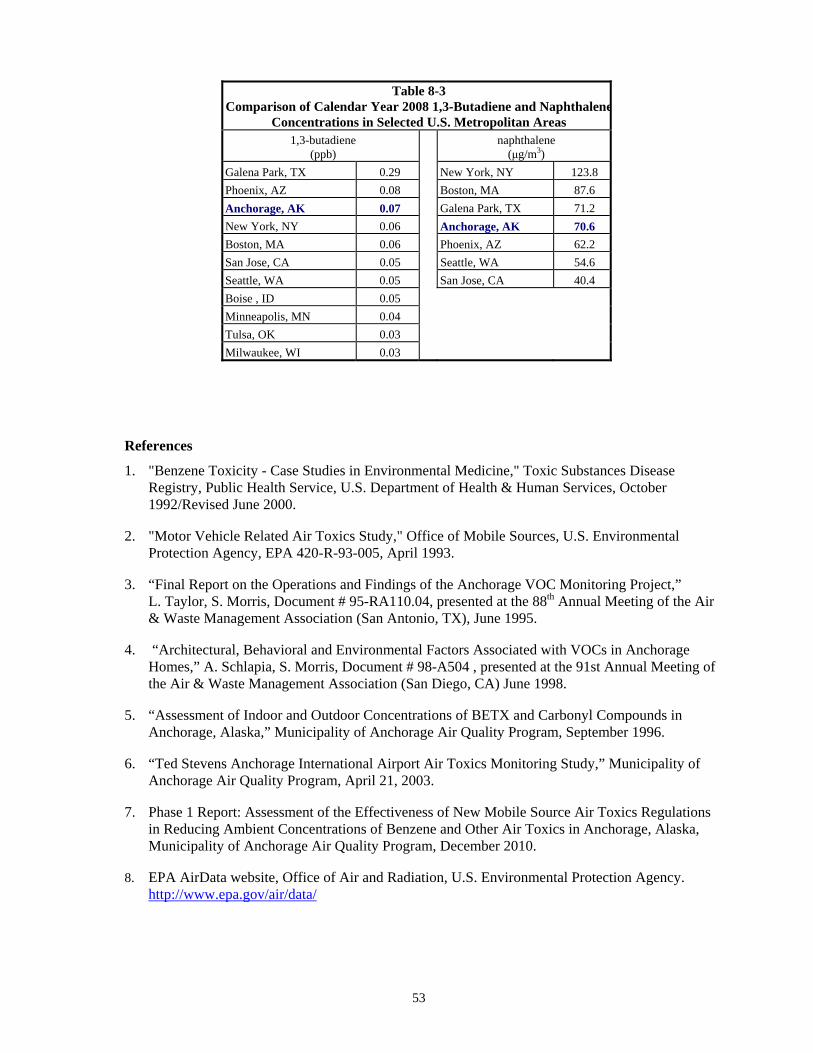
53

Table 8-3 Comparison of Calendar Year 2008 1,3-Butadiene and Naphthalene

Concentrations in Selected U.S. Metropolitan Areas 1,3-butadiene

(ppb) naphthalene

(μg/m3) Galena Park, TX 0.29 New York, NY 123.8 Phoenix, AZ 0.08 Boston, MA 87.6 Anchorage, AK 0.07 Galena Park, TX 71.2 New York, NY 0.06 Anchorage, AK 70.6 Boston, MA 0.06 Phoenix, AZ 62.2 San Jose, CA 0.05 Seattle, WA 54.6 Seattle, WA 0.05 San Jose, CA 40.4 Boise , ID 0.05 Minneapolis, MN 0.04 Tulsa, OK 0.03 Milwaukee, WI 0.03

References

1. "Benzene Toxicity - Case Studies in Environmental Medicine," Toxic Substances Disease Registry, Public Health Service, U.S. Department of Health & Human Services, October 1992/Revised June 2000.

2. "Motor Vehicle Related Air Toxics Study," Office of Mobile Sources, U.S. Environmental Protection Agency, EPA 420-R-93-005, April 1993.

3. “Final Report on the Operations and Findings of the Anchorage VOC Monitoring Project,” L. Taylor, S. Morris, Document # 95-RA110.04, presented at the 88th Annual Meeting of the Air & Waste Management Association (San Antonio, TX), June 1995.

4. “Architectural, Behavioral and Environmental Factors Associated with VOCs in Anchorage Homes,” A. Schlapia, S. Morris, Document # 98-A504 , presented at the 91st Annual Meeting of the Air & Waste Management Association (San Diego, CA) June 1998.

5. “Assessment of Indoor and Outdoor Concentrations of BETX and Carbonyl Compounds in Anchorage, Alaska,” Municipality of Anchorage Air Quality Program, September 1996.

6. “Ted Stevens Anchorage International Airport Air Toxics Monitoring Study,” Municipality of Anchorage Air Quality Program, April 21, 2003.

7. Phase 1 Report: Assessment of the Effectiveness of New Mobile Source Air Toxics Regulations in Reducing Ambient Concentrations of Benzene and Other Air Toxics in Anchorage, Alaska, Municipality of Anchorage Air Quality Program, December 2010.

8. EPA AirData website, Office of Air and Radiation, U.S. Environmental Protection Agency. http://www.epa.gov/air/data/