air pollution, health, and socio-economic status: the

Journal of Health Economics 23 (2004) 1209–1236

Air pollution, health, and socio-economic status: theeffect of outdoor air quality on childhood asthma

Matthew J. Neidell∗

University of Chicago, CISES, 5734 S. Ellis Ave., Chicago, IL 60637, USA

Received 1 August 2003; received in revised form 1 April 2004; accepted 1 May 2004

Abstract

This paper estimates the effect of air pollution on child hospitalizations for asthma using naturallyoccurring seasonal variations in pollution within zip codes. Of the pollutants considered, carbonmonoxide (CO) has a significant effect on asthma for children ages 1–18: if 1998 pollution levelswere at their 1992 levels, there would be a 5–14% increase in asthma admissions. Also, householdsrespond to information about pollution with avoidance behavior, suggesting it is important to accountfor these endogenous responses when measuring the effect of pollution on health. Finally, the effectof pollution is greater for children of lower socio-economic status (SES), indicating that pollution isone potential mechanism by which SES affects health.© 2004 Elsevier B.V. All rights reserved.

JEL classification:I12; J13; J15; Q25

Keywords:Pollution; Health; Asthma; Socio-economic status; Avoidance behavior; Zip code fixed effect

1. Introduction

A primary objective of air quality policies around the world is to protect human health.However, many critics argue that air quality standards are set somewhat arbitrarily with in-conclusive evidence of the specific health benefits and with inadequate considerations of the

∗ Tel.: +1 773 834 9945; fax: +1 773 834 1045.E-mail address:[email protected].

0167-6296/$ – see front matter © 2004 Elsevier B.V. All rights reserved.doi:10.1016/j.jhealeco.2004.05.002

1210 M.J. Neidell / Journal of Health Economics 23 (2004) 1209–1236

costs to producers. Given that substantial costs to industry have been widely demonstrated,1

in order to determine optimal policy intervention it is crucial to identify the associated ben-efits from improvements in air quality.

While many studies have focused on estimating a relationship between pollution andhealth, they have largely neglected to consider that pollution exposure is endogenouslydetermined if individuals make choices to maximize their well being. People with highpreferences for clean air may choose to live in areas with better air quality. People canrespond to a wide range of readily available information on pollution levels by adjusting theirexposure. Failing to appropriately account for such actions can yield misleading estimatesof the causal effect of pollution on health.

This paper focuses on developing an empirical strategy for measuring the effect of pollu-tion on health. Specifically, I look at the effect of air pollution on children’s hospitalizationfor asthma. Childhood asthma is of particular interest for two reasons: (1) asthma is the lead-ing chronic condition affecting children; and (2) current pollution standards are based onadult health responses to pollution and children face a greater risk from pollution exposuredue to the sensitivity of their developing biological systems.

This study builds on earlier work in five ways. One, I develop a unique, monthly, zipcode level data set by matching information about all individual hospitalizations in Califor-nia between 1992 and 1998 to ambient pollution levels, meteorological data, and variousdemographic data. Two, I identify the effect of pollution using naturally occurring seasonalvariations within zip codes. Since zip codes are a finely defined geographic area and theseasonal patterns in pollution are remarkably strong and diverse throughout California, thiscontrols for many confounding factors that might affect asthma hospitalization rates. Three,I allow the effect of pollution to differ with the age of the child, as biological models suggestit might. Four, I collect data about public announcements of “smog alerts” in order to showempirically that it is important to account for the endogeneity of household responses topollution. Five, to assess if the effect of pollution varies across different segments of thepopulation, I allow the effect of pollution to differ with socio-economic status (SES), asmeasured by education levels in the zip code.

The primary finding of this paper is that of the pollutants considered, carbon monoxide(CO) has a significant effect on hospitalizations for asthma among children ages 1–18, whilenone of the pollutants considered has a clear impact on hospitalizations for infants. Thisdiscrepancy across age groups is possibly due to the complications inherent in diagnosingasthma in infants or differing degrees of avoidance behavior by age. The decline in pollutionlevels from 1992 to 1998 decreased asthma rates by between 5 and 14%, resulting in a savingsof approximately $5.2 million in hospital expenses for asthma admissions in California in1998 alone.

A second finding is that families display avoidance behavior by responding to smogalerts, indicating the importance of accounting for the endogeneity of family behaviorwhen measuring the causal effect of pollution on health. The announcement of smog alertsdecreases asthma hospitalizations by roughly 1%, while including these announcementsraises the effect of O3 on admissions, although O3 does not appear to significantly affect

1 See, for example,Greenstone (2002)for estimates on the costs of the Clean Air Acts on industrial activity inthe United States.

M.J. Neidell / Journal of Health Economics 23 (2004) 1209–1236 1211

admissions. This suggests that omitting avoidance behavior yields estimates that are a lowerbound of the biological effect of pollution on health.

Third, not only are the coefficients measuring the effect of pollution larger for low SESchildren, but these children are also exposed to considerably higher levels of pollution. As aresult, they suffer greater harm from pollution, although higher pollution levels explain onlyas much as 6% of the gap in admission rates for asthma. Although there are many remainingfactors for explaining this gap, this suggests that pollution is one potential mechanism forthe well-known relationship between SES and health—poorer families are unable to affordto live in cleaner areas, and their children’s health suffers as a result.

The paper is laid out as follows. Section2 provides some background information onasthma and its potential association with pollution. Section3 discusses the conceptualframework and estimation strategy. Section4 describes the data used for the analysis.Section5 presents the econometric results. Section6 concludes with a discussion.

2. Background

Approximately 5 million children in the United States have asthma. It is the leadingspecific reason for school absence and the most frequent cause of pediatric emergencyroom use and hospital admission (National Institute of Environmental Health Sciences,1/2000). Asthma disproportionately attacks children of lower SES, and continues for mostwell beyond childhood (American Academy of Pediatrics, 2000). Most disconcerting is thatreported asthma rates for children age 18 and younger have increased by more than 70%from 1982 to 1994 (American Academy of Pediatrics, 2000)2.

Despite mounting public concern, the factors influencing this illness are not fully un-derstood, especially for children. Medical research has demonstrated that asthma is botha chronic and acute illness. In the chronic aspect, an individual’s airways are persistentlyinflamed and their immune system is hyper-responsive, but the causes of this remain largelyunknown (American Lung Association, 2000). During an acute response, an irritant is in-haled that causes three changes to occur: muscular bands around the bronchioles constrict,the linings of the airway become inflamed, and excess mucus is produced. The irritantsare believed to cause this because, by being recognized by the immune system as for-eign, immunoglobin E (IgE), an antibody, is produced in response. IgE binds with mastcells—particular cells filled with chemical mediators, causing the release of some of themediators in the mast cells (American Academy of Pediatrics, 2000). As a result of thesechanges in lung functioning, the airways are severely narrowed, and, by making it difficultto breathe, may lead to an asthma attack.

While there are many potential irritants3, or asthma “triggers”, outdoor air pollutionhas long been suspected a major culprit. Carbon monoxide is an odorless, colorless gasthat bonds with hemoglobin more easily than oxygen, so that it reduces the body’s abilityto deliver oxygen to organs and tissues. Although the biological plausibility of a directeffect of CO on asthma is unlikely, because CO mainly comes from vehicle exhaust, a

2 There is, however, much debate regarding this apparent rise in asthma. I discuss this is more detail below.3 These include include molds, pollens, animal dander, tobacco smoke, weather, and exercise.


likely explanation is that CO functions as a proxy for vehicle emissions (U.S. EPA, 2000).Nitrogen dioxide (NO2) is a brown, reactive gas that irritates the lungs and may lowerresistance to respiratory infections. Particulate matter (PM10), which can take many forms,including ash and dust, is believed to cause the most damage from the smallest particles,since they are inhaled deep into the lungs (U.S. EPA, 2003). The mechanisms throughwhich particles harm health are controversial, however the leading theory is that they causean inflammatory response, which weakens the immune system (Seaton, 1995). Ozone (O3),the major component of urban smog, is a highly reactive compound that damages tissue,reduces lung function, and sensitizes the lungs to other irritants. Motor vehicles are a majorsource of PM10, NO2, and especially of CO; as much as 90% of CO in cities comes frommotor vehicle exhaust (U.S. EPA, 2000), while O3 is formed through reactions betweennitrogen oxides (such as NO2) and volatile organic compounds (which are found in autoemissions, among other sources) in heat and sunlight.

Many researchers have attempted to estimate the link between these pollutants and child-hood asthma, but with mixed results.4 Most studies have been short time-series that focuson a given city and track the daily number of hospital or emergency room (ER) admissionsfor asthma and the average daily levels of various criteria pollutants.5 A wide range ofestimated correlations between admissions for asthma and CO, O3, PM10, and NO2 havebeen reported, with no clear patterns or magnitude of effects evident.6

Due to the inconclusive findings and the fact that ambient air pollution levels havedeclined in most parts of the country while the reported incidence of asthma has risen7,many researchers have begun to question the link between ambient air pollution and asthma(von Mutius, 2000a, 2000b; Vacek, 1999; Duhme et al., 1998). For example, the Committeeon the Medical Effects of Air Pollution (Committee on the Medical Effects of Air Pollution,2000) concluded that “overall evidence is small that non-biological outdoor air pollutionhas an important effect on the initiation and [provocation] of asthma”, (2000). As a result,alternative theories have sprung up recently. One theory proposes that children are “tooclean” because they often use antibiotics to combat minor illnesses. As a result, their immunesystems do not develop properly and attack many harmless substances that enter the body(American Academy of Pediatrics, 2000). A second competing theory is that the changinglifestyles of children—poorer diets, less exercise, more time indoors - has led to the increasein asthma related illnesses (von Mutius, 2000a).

However, not all researchers have dismissed the role that pollution may play. There isa debate as to whether asthma rates have actually increased. Better detection of asthma

4 Some representative studies includeDesqueyroux and Momas (1999), Gouveia and Fletcher (2000), Fauroux(2000), Garty et al. (1998), Krupnick et al. (1990)andNorris et al. (1999).

5 Criteria pollutants are non-toxic air pollutants considered most responsible for urban air pollution and areknown to be hazardous to health. They include SO2, NO2, O3, CO, PM10, and lead.

6 Other studies that have attempted to link pollution and general health use data that follow the same individualsover a short period of time to control for permanent health-related factors, such as smoking rates and exercisehabits (Alberini and Krupnick, 1998; Portney and Mullahy, 1986, 1990). However, most of these studies focus onadults, and the results may not be directly applicable to children. Furthermore, a general limitation of these studiesis that, given the limited number of observations over a short period of time, it is unlikely that there is enoughvariation in specific health outcomes, such as asthma, to obtain precise estimates.

7 See footnote 2.


and different classifications of illness could explain some of the increases in individual anddoctor reports. For example, what was long labeled wheezy bronchitis is now classifiedas asthma (Speizer, 2001). Recent expansions in Medicaid could also explain part of theincrease in reported cases – as children’s access to health care increases, there is a greaterchance of early detection and treatment.

Many researchers have also questioned the methodological approaches used to iden-tify the relationship between pollution and asthma (Nystad, 2000; Eggleston et al., 1999;von Mutius, 2000b; Bjorksten, 1999). Since air pollution is not randomly assigned, moststudies have been largely unsuccessful in disentangling pollution from other confoundingfactors that affect health. Additionally, these studies do not account for direct responses toambient levels of pollution. Furthermore, these studies tend to group all children into justone category, and we might expect a number of biological and behavioral factors to varyfor children of different ages. Lastly, most studies conduct single pollutant analyses, whichdoes not provide clear policy implications if pollutants are highly correlated.

A final reason to believe a connection between pollution and asthma might exist is thatstudies with more convincing empirical designs have found consistent effects of pollutionon children’s health.Chay and Greenstone (2003)use declines in pollution that resultedfrom the 1980–82 recessions and find a strong link between total suspended particles andinfant mortality. Since most infant mortality is due to respiratory failure, it is reasonable tosuspect that pollution could be related to other respiratory illnesses, such as asthma.Ransomand Pope (1995)use changes in pollution that resulted from the opening and closing of asteel mill due to a labor strike and find a large effect on bronchitis and asthma in children.Their study, however, does not identify the effect of specific pollutants, only the effect ofthe mill being opened or closed.8

3. Conceptual framework

One approach to understanding the impact of pollution on health would be to assumethat everyone is unaware of the amount of pollution in the air. Therefore, ambient levels ofpollution would serve as an unbiased proxy for an individual’s exposure to pollution andpollution levels would not be correlated with any types of behavior. One could then estimatea relationship between health and pollution by regressing health outcomes on ambient levelsof pollution as well as other exogenous factors that are related to both pollution and health,such as weather conditions.

However, this approach is oversimplified because individuals can undertake avoidanceactivities to reduce the effect of externalities, which makes an individual’s exposure topollution an endogenously determined variable.9 This introduces two issues. First, thereare many tools available to inform people when air pollution levels pose a threat to health.

8 Another study (Friedman et al., 2001) that attempts to use a “natural experiment” caused by changing trafficpatterns in Atlanta during the 1996 Olympics also does not identify the effects of particular pollutants. Moreover,this study does not consider the changing behavior of families in response to the Olympics in general.

9 For a detailed description of avoidance (or averting) behavior, seeZeckhauser and Fisher (1976)orBresnahanet al. (1997).


Home devices, such as peak expiratory flow (PEF) meters, can be used to measure lungfunctioning on a given day (if the individual already has a respiratory illness). CaliforniaState law requires the announcement of air quality episodes, or “smog alerts”, when pollutionlevels are predicted to exceed certain limits (Air Resources Board, 1990). State and localagencies are required to report a daily measure of air quality in large metropolitan areas,with newspapers a common source (U.S. EPA, 1999a). Many regional air quality offices,such as the California Air Resources Board, provide web pages with up-to-the-minutepollution details and e-mail notifications of dangerous pollution levels.10 Many pollutantsare directly visible – on high-smog days in Los Angeles, whitish clouds often cover thesky or a reddish-brown haze is visible around the horizon. If people directly respond to thisinformation, then ambient pollution levels will not accurately represent their exposure topollution.

A second issue arises because air quality, like many local public goods, is capitalizedinto housing prices, making it an attribute of a home that people can demand (Chay andGreenstone, 2000). Therefore, families with a higher value for cleaner air can locate inareas with better air quality.11 These families may also make additional investments in theirchildren’s health – they may be less likely to smoke or more likely to seek preventativehealth care and have an existing relationship with a doctor. As a result, there are manyconfounding behavioral factors related to both pollution and health, making it difficult toidentify the effect of pollution on health.12

Additionally, parents’ investment decisions and pollution exposure may vary dependingon the health stock or age of their child. This could occur because some children face agreater risk from the same exposure as other children or the costs to monitor behavior varyby child or age. For example, it is not uncommon for parents to insist on keeping tobaccosmoke away from their infant, only to become more yielding as the child grows older,suggesting avoidance behavior might be more actively undertaken for younger children.Therefore, a specific child’s exposure to pollution is potentially related to both the familyspecific endowment and type of care utilized.

These issues suggest that the ambient levels of pollution where a child lives are potentiallyrelated to many broadly defined factors that are difficult to fully observe, and omitting themfrom a regression could cause biased estimates of ambient pollution on asthma. I proposeto control for these variables using the following innovations. First, I look at the effectof air pollution separately for children of different age groups. These groups correspondwith both biological development and the type of care that families typically display towardschildren. I define the age categories of interest as follows: children age 0–1 (lung “branching”occurring at rapid rate; infants most protected by parents and most likely to use hospitalfor illness); 1–3 (alveoli develop and mature; children spend more time in day care); 3–6(children more likely to enroll in preschool/kindergarten); 6–12 (elementary school); and

10 For example, visithttp://www.epa.gov/airnow/to find daily pollution levels throughout the United States.11 Families do not need to have direct preferences for this attribute. However, because air quality is an input in

the health production function, people with preferences regarding health will have implicit tastes for air quality.12 This is analogous to the confounding that arises in estimating the effect of school quality on test scores.

Parents who choose to live in areas with better school quality may also make additional investments in theirchildren, making it difficult to identify the effect of school quality.

http://www.epa.gov/airnow/


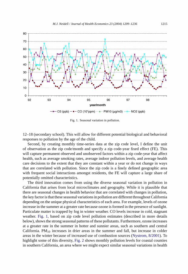
Fig. 1. Seasonal variation in pollution.

12–18 (secondary school). This will allow for different potential biological and behavioralresponses to pollution by the age of the child.

Second, by creating monthly time-series data at the zip code level, I define the unitof observation as the zip code/month and specify a zip code-year fixed effect (FE). Thiswill capture permanent observed and unobserved factors within a zip code-year that affecthealth, such as average smoking rates, average indoor pollution levels, and average healthcare decisions to the extent that they are constant within a year or do not change in waysthat are correlated with pollution. Since the zip code is a finely defined geographic areawith frequent social interactions amongst residents, the FE will capture a large share ofpotentially omitted characteristics.

The third innovation comes from using the diverse seasonal variation in pollution inCalifornia that arises from local microclimates and geography. While it is plausible thatthere are seasonal changes in health behavior that are correlated with changes in pollution,the key factor is that these seasonal variations in pollution are different throughout Californiadepending on the unique physical characteristics of each area. For example, levels of ozoneincrease in the summer at a greater rate because ozone is formed in the presence of sunlight.Particulate matter is trapped by fog in winter weather. CO levels increase in cold, stagnantweather.Fig. 1, based on zip code level pollution estimates (described in more detailsbelow), shows the strong seasonal patterns of these pollutants. Furthermore, ozone increasesat a greater rate in the summer in hotter and sunnier areas, such as southern and centralCalifornia. PM10 increases in drier areas in the summer and fall, but increase in colderareas in the winter because of increased use of combustion sources (Nystrom, 8/2001). Tohighlight some of this diversity,Fig. 2shows monthly pollution levels for coastal countiesin southern California, an area where we might expect similar seasonal variations in health


Fig

.2.

Sea

sona

lvar

iatio

nin

pollu

tion

byco

unty

.


behavior and face comparable weather patterns. Focusing on ozone, Los Angeles and Orangecounties have comparable levels in the winter, but Los Angeles experiences higher levelsin the summer. Meanwhile, San Diego experiences higher winter levels that Los Angelesand Orange, but lower summer levels. Since these patterns in pollution vary throughoutCalifornia and are naturally occurring, it is reasonable to assume that they are independentof many seasonal investments in health.

In sum, I will compare how seasonal changes in pollution within a given zip code-yearaffect changes in seasonal asthma rates for a specific age group.13 The following exampleof smoking rates and outdoor pollution highlights how the empirical strategy works. Failingto control for smoking is only a problem if smoking behavior is related to both pollutionand asthma. By looking at separate age groups, I circumvent the need to control for howparents monitor tobacco smoke around their children based on the age of the child. By usingzip code-year fixed effects, I look at whether changes in pollution are linked to changes inasthma within a zip code for each year. If smoking either does not change with changes inpollution, or if it changes in a way that is unrelated to changes in pollution, then the fixedeffect would control for smoking behavior. Smoking behavior, however, may change withina year - people may be more likely to smoke when they spend more time outside as theweather improves. If this is the case, the fixed effect will not capture the changing smokingpatterns. However, if smoking patterns do not change from one season to the next in a waythat is correlated with the seasonal changes in pollution unique to that area, then I will notneed to explicitly control for smoking behavior.

While this identification strategy overcomes many problems, there is one main sourceof endogeneity that remains—contemporaneous avoidance behavior. Since people can di-rectly respond to daily pollution, this will not be captured by the identification strategy.Although I include some measures of avoidance behavior, these measures only capturepart of avoidance behavior and only as it relates to ozone. However, if contemporaneousavoidance behavior is positively related to pollution levels and avoidance behavior lowersthe likelihood of having an asthma attack, omitting it will yield a lower bound of the trueeffect.

To proceed with estimation, I estimate the following model separately for each age group:

Yzyt = β0Pzyt + β1Azyt + β2Xzyt + αzy + ηyt + εzyt (1)

where the subscripts z, y, and t indicate zip code, year, and month, respectively,Y is thenumber of ER asthma admissions,Pare ambient air pollution levels,A is contemporaneousavoidance behavior that directly affects the child’s exposure to pollution,Xare other factorsthat affect health (such as weather), and� is an i.i.d. error term. The key identificationparameters areαzy, zip code-year fixed effects, andηyt, year-month dummy variables.β0is the coefficient vector of interest. The main hypothesis to test is whetherβ0 =0, namelythat pollution has no effect on asthma admissions.

13 One notable limitation of using seasonal changes in pollution is that, by smoothing out daily variation,some valuable information may be lost. However, this only affects the efficiency of the estimates unless there arethreshold effects such that pollution beyond a certain level induces asthma attacks. Additionally, using seasonalvariation will not provide evidence on long-term health effects.


4. Data

4.1. Sources

The California Hospital Discharge Data (CHDD) is a rich source of individual healthoutcomes. This data set records the principal diagnosis of the patient upon release from thehospital14, the month of admission,15 the zip code of residence, as well as the sex, race, age,and the expected source of payment for all individuals discharged from a hospital in thestate of California. Data are available from 1992 to 1998 and each year contains on averageover 800,000 hospital discharges for children under age 18 (not including newborns).

While hospital data does not include information on all asthma attacks, the CHDD offersthree key advantages over self-reported surveys. First, hospital discharges, in particular ERadmissions, are a more objective measure of asthma and are less likely to be sensitive toreporting biases.16 Second, there are a large number of observations available each year inthe CHDD. Third, having the zip code of the patient enables me to specify a zip code fixedeffect and to merge other key data sources at the zip code level.

The key data merged are atmospheric pollution levels from Environmental ProtectionAgency (EPA) air monitoring stations throughout California. The monitor data are readilyavailable from 1982 until the present and are the most detailed data recording ambientlevels of criteria pollutants. Furthermore, they contain the exact location of the monitor,enabling them to be merged with the CHDD.Fig. 3 shows O3 monitors in California in1999 along with county outlines. These monitors are mainly located in the more denselypopulated areas (shaded in gray).Fig. 4highlights Los Angeles County, showing again O3monitors and now the outlines of zip codes. Since Los Angeles is a diverse county bothdemographically and geographically and there are many monitors to capture local pollutionlevels, assigning pollution at the zip code level should produce more reliable measures thanfrom assigning it at a broader level.

I also merge other data sources at the zip code level. Monthly meteorological data fromthe National Climatic Data Center contains various measures from more than 1000 weatherstations in California as well as their exact location.17The California Association of Realtorsprovides monthly zip code level information on the number of homes and average andmedian sales price from 1991 to the present. Using 1990 Census estimates of populationcounts by age for each zip code and annual county estimates by age from the DemographicResearch Unit of the California Department of Finance, I have approximated the annualpopulation for each zip code and age group.

As proxies for avoidance behavior, I merge the number of smog alerts announced in eachmonth. Air quality episodes, or “smog alerts”, are required by California law to be issued by

14 This is assigned according to the International Classification of Diseases, 9th Revision, Clinical Modification(ICD- 9-CM) by the U.S. Department of Health and Human Services.

15 The exact day of the month is censored in the version of the data that has already been released to me. Onlyan indicator for the day of the week is available.

16 ER admissions account for approximately 67% of all hospital admissions for asthma. When performing theanalysis using all hospital admissions, the results did not change considerably.

17 The meterological data are merged using the same inverse-distance weighted technique used to approximatezip code levels of pollution (described below).


Fig. 3. Ozone monitors in California.

local air quality management districts (AQMD)18 when criteria pollutants exceed levels asspecified by the California Air Resources Board.19 When this occurs, schools are directlycontacted and are urged to limit physical activities for children until pollution levels ease,while other sensitive people are advised to avoid the pollution by remaining indoors (AirResources Board, 1990). While these advisories are required to be announced for all of thecriteria pollutants, historically announcements have only be made for ozone levels, and asa result the advisories are commonly referred to as “smog alerts.”

4.2. Linking pollution

To approximate a monthly time-series of pollution at the zip code level, I first calculatedthe coordinates for the centroid of each zip code in California. Using the reported coordinatesof the EPA monitors, I then measured the distance between each centroid and each monitor.Finally, I calculated the level of pollution for a zip code by averaging reported values fromall monitors within 20 miles of the centroid, weighting by the inverse of the distance from

18 There are currently 17 air quality management districts in California.19 While I only possess this data for the AQMD that covers Los Angeles, Orange, Riverside and San Bernardino

counties, it is unlikely that any other area has experienced smog alerts during this period.


Fig. 4. Ozone monitors in Los Angeles county.

the centroid to the monitor. Therefore, I define pollution in zip code z at timeyt as:

Pzyt =∑

j

((Pjyt × 1/(Dj|Dj ≤ 20))

1/(Dj|Dj ≤ 20)

)(2)

whereDj is the distance from monitorj to the centroid of zip code z andPjzt is the pollutionmeasure at monitorj in year y in month t.

Five immediate issues arise in measuring pollution in this way. First, the choice of 20miles as the cutoff is arbitrary. To test the sensitivity of this assumption, I also assignedpollution levels using distance cutoffs of 10 and 5 miles. Panel A of appendix Table A.1shows the correlation between pollution levels calculated using the various cut-offs. Thesecorrelations are remarkably high, with none below 0.95, suggesting that the choice ofdistance is unlikely to introduce any biases.20

Second, many monitors have been added or removed over the time period studied. Thisoccurs because pollution monitors are installed in areas where pollution exceeds NAAQS,and can also be removed from an area if it falls below NAAQS (U.S. EPA, 1999b). As a result,monitors are more likely to be placed in areas where pollution levels have been increasing,and less likely to exist in areas where pollution has been declining. To assess the implication

20 When performing the analysis using a distance of 10 or 5 miles, the results were nearly identical, consistentwith these high correlations.


of this, I estimate (2) in two ways: using all monitors from 1992 to 1998 and using onlycontinuously operated monitors from 1992 to 1998. Panel B of appendix Table A.1 showsthe number of monitors over time for both methods and the correlation between monthly zipcode levels of each pollutant calculated by each method. The overall number of monitorshas not changed considerably and the correlations for all are at least 0.98, indicating thatthe sampling technique used for monitors should not interfere with inference.

Third, there are many factors that affect how pollutants travel, such as wind, rain, and thesize of the pollutant particle, and this may affect how well (2) measures the actual pollutionconcentration21. For example, particulate matter, such as PM10, settles to the ground at amuch quicker rate than do gaseous pollutants (Wilson and Spengler, 1996). To get a senseof how accurate the above approach is, I estimate the level of pollution at each monitor (asopposed to zip code) using the above formula as if the monitor of interest were not there.Therefore, I estimate the amount of pollution at a given monitor based on the pollutionlevels at monitors less than 20 miles away. I do this for all monitors and then calculatethe correlation between the estimated pollution and the actual pollution, shown in panel Cof appendix Table A.1. The correlations for O3 and NO2 are remarkably high. This is notsurprising for O3 given it is formed in the atmosphere, as opposed to being directly emitted.For PM10 and CO, the correlations are slightly lower, but still quite high at over 0.75. Thisindicates the reasonable accuracy of this method for assigning pollution and suggests itdoes not appear to be a major concern for this analysis.

Fourth, while it is crucial to control for multiple pollutants simultaneously, trying toseparately identify the effect of each pollutant can be difficult if pollutants are highlycorrelated. Many pollutants originate from similar sources, as the preceding chart indicated.Appendix Table A.2 shows the correlation matrix for the pollutants as assigned accordingto (2). O3 does not appear highly correlated with any other pollutants, while NO2 appearshighly correlated with CO and PM10. This may make it difficult to obtain precise estimatesfor NO2, making it useful to analyze models with the pollutants included individually.

Fifth, since monitors tend to exist in more polluted and populated areas, it is important tounderstand how the characteristics of the population in these areas differ from those that areexcluded from the analysis. Appendix Table A.3 shows various demographic characteristicsfor zip codes that are within 20 miles of a monitor for each of the pollutants and zip codesthat are not. While all of the variables shown are statistically different, the driving forcebehind these differences appears to be the percent of the population of the zip code that livesin urbanized areas. This coincides with the monitor locations shown inFig. 3. Although thislimits the representativeness of these findings, rural areas represent a much lower fractionof the population and are less likely to experience high levels of pollution.

4.3. Trends and descriptive statistics

Table 1panel A shows the descriptive statistics of the data used in the analysis, includingthe “between” and “within” zip code-year variation of each variable.22 For the pollutants,

21 While I obtained measures of precipitation to include in the analysis, wind data is not as widely available.Furthermore, there is much debate on how to incorporate wind data.

22 The “between” standard deviation is calculated using ¯xi and the “within” is calculated usingx = x̄i + x̄.

1222M.J.N

eidell/Jo

urnalo

fHealth

Eco

nomics

23(2004)1209–1236

Table 1Summary statistics

A. Summary statistics

Observations Groups Mean S.D. ‘Between’ zip-year S.D. ‘Within’ zip-year S.D.

O3 (ppb) 54,963 4991 38.905 17.803 9.830 14.855CO (ppm) 54,963 4991 1.777 1.037 0.679 0.790PM10 (�g/m3) 54,963 4991 34.210 13.984 9.874 9.933NO2 (ppb) 54,963 4991 45.947 17.171 14.392 9.539ER asthma rate age 0–1 54,843 4979 0.431 1.572 0.964 1.382Population age 0–1 54,843 4979 578 390 391 0ER asthma rate age 1–3 43,624 4949 0.135 0.755 0.469 0.668Population age 1–3 43,624 4949 2347 1449 1416 0ER asthma rate age 3–6 44,462 4959 0.167 1.066 0.762 0.916Population age 3–6 44,462 4959 2159 1327 1305 0ER asthma rate age 6–12 50,602 4987 0.088 0.393 0.313 0.344Population age 6–12 50,602 4987 3568 2209 2221 0ER asthma rate age 12–18 55,377 4990 0.072 0.411 0.202 0.380Population age 12–18 55,377 4990 1812 1159 1170 0% Normal neonates 54,963 4991 0.698 0.078 0.075 0.020% Government insurance 54,962 4990 0.399 0.216 0.216 0.023Ave. max. temperature (◦F) 54,963 4991 0.073 0.011 0.004 0.010Total precipitation (in.) 54,963 4991 0.007 0.011 0.003 0.010Semi-annual house price 45,662 4194 20,007 12,197 11,841 5.503Smog alerts 54,963 4991 0.288 1.582 0.808 1.353

B. Pollution and asthma by SES

Pollutant High Low Age High Low

O3 38.283 (0.123) 40.117 (0.138) 0–1 0.493 (0.011) 0.729 (0.015)CO 1.652 (0.007) 1.953 (0.008) 1–3 0.177 (0.004) 0.179 (0.009)PM10 31.851 (0.095) 38.160 (0.104) 3–6 0.193 (0.004) 0.235 (0.012)NO2 42.964 (0.118) 50.361 (0.123) 6–12 0.102 (0.002) 0.127 (0.004)Observations 19,458 19,299 12–18 0.122 (0.003) 0.130 (0.005)

Note: The “between” standard deviation is calculated using ¯xi and the “within” is calculated using ¯xit − x̄i + x̄. Standard errors in parenthesis. Low SES is defined aszip code percentage of high school dropouts greater than the median level of high school dropouts.


it is not unusual for the within zip code variation to exceed the between zip code variation,as is the case for O3 and CO. For asthma admission rates,23 younger children have a greaterlikelihood of visiting the ER,24 with infants approximately six times more likely to visit theER than children over 6 and 1–6 year-olds two times more likely to visit than children over6. Most of the variation in asthma rates comes from within the zip code-year. The patterns invariation for asthma and pollution suggest ample variation for obtaining precise estimatesusing the identification strategy described above.

Table 1panel A also shows variables that representAzyt andXzyt. House prices aredesigned to reflect changes in asset wealth and are a “sufficient” statistics for many de-mographics of a given area, such as school quality and crime rates. The percentage ofnewborns with government-sponsored health insurance (calculated from the CHDD) isused as a measure of changes in the bottom of the income distribution.25 The percentage ofnormal newborns (calculated from the CHDD26) is used to approximate the health stock forinfants. Monthly hospital admissions for influenza are included to control for co-morbiditiesthat may be inducing asthma episodes, rather than pollution itself. Average maximum tem-perature and inches of precipitation both affect the likelihood of being outdoors and maydirectly exacerbate asthma symptoms (American Lung Association, 8/2001).

Since asthma disproportionately attacks children of low SES,Table 1panel B showspollution levels and ER asthma rates for two SES groups. I define SES groups as aboveand below the median for the percent of adults over 25 years old in a zip code without ahigh school diploma. The average levels of all pollutants are higher for the low SES groups.Asthma rates for low SES are almost twice as high as high SES for infants, but are onlyslightly higher for children over age 1. These differences in pollution and asthma rates bySES are statistically significant, except for asthma for age 1–3.27

In turning to annual trends,Fig. 5shows asthma patterns in California and other regionsin the United States using the National Hospital Discharge Survey (NHDS).28 The northeasthas the highest admission rate, followed by the Midwest, the south, and then the west. Thepattern for California is similar to that for the entire United States, but at a level that is almost50% lower. In turning to monthly patterns,Fig. 6shows asthma patterns over time for eachage group separately. Immediately evident are the strong seasonal patterns for admissionsfor all age groups. Rates for each age group increase on average anywhere from two to threetimes from the lowest month to the highest. Furthermore, the seasonal patterns differ across

23 Asthma is labeled as ICD-9-CM 493.24 ER admissions are distinguished from other admissions according to the “source of admission” variable from

the CHDD.25 There was only one expansion in medicaid eligibility that affected newborns during the time period studied.

In February of 1995, eligibility was extended from 185 to 200% of the federal poverty level. Although Access toInfants and Mothers (AIM) also increased during this period, less than 0.6% of all births in California are paid forby AIM (Managed Risk Medical Insurance Board, 8/2001).

26 In the CHDD, newborns are classified into one of the following seven categories: (1) died or transferred (2)extreme immaturity or respiratory distress syndrome (3) prematurity with major problems (4) prematurity withoutmajor problems (5) full term with major problems (6) neonate with other significant problems and (7) normalnewborn.

27 These patterns are also present when SES is defined by race or income.28 The NHDS does not provide information to separately identify emergency and non-emergency hospital

admissions and the only geographic identifier is the region.


Fig. 5. All hospital admissions for asthma for children in U.S.

age groups. The high season for infants is the winter, whereas high season for teens is thefall. These striking patterns demonstrate the importance of looking at age groups separatelyand the potential value in exploiting seasonal variation.

Before turning to the estimation, a case study of a specific zip code highlights the mainfindings of this analysis.Fig. 7 plots monthly standardized pollution levels and asthmacounts for children ages 3–6 in zip code 92335 (Fontana in San Bernardino County)).A strong pattern between asthma and CO emerges, with peaks and trough occurring atroughly the same time throughout the entire time period. Asthma and O3 appear negativelycorrelated, with O3 peaking in the summer. While at times asthma follows the patternsof PM10 and NO2, the pattern tends not to persist for the entire time period, indicating apotential link between CO and asthma.

Fig. 6. Monthly ER asthma rates by age.


Fig

.7.

Pol

luto

nan

das

thm

afo

rag

es3-

6in

Zip

9233

5.


5. Results

5.1. Main results

The first set of results, fixed effect estimates of Eq.(1) without any direct controls foravoidance behavior, indicate that pollution has a differential impact on infants as comparedto older children. As indicated inTable 2panel A,29 none of the pollutants are significantlyrelated to asthma ER hospitalizations for infants. However, for all older age groups, COis positive and significantly correlated with asthma. One explanation for the differenceacross age groups is that asthma is often difficult to precisely identify in infants because ofcommunication limitations, little history of respiratory illnesses, and birth complications(Letourneau et al., 1992). O3 has a negative effect on admissions, and is precisely estimatedfor ages 6–12. NO2 and PM10 are generally positively correlated with asthma, but only NO2is significant for Ages 6–12.

In terms of the control variables, temperature and precipitation are negatively correlatedwith asthma. While weather may have a direct effect on asthma, such as precipitation “clean-ing” the air (Wilson and Spengler, 1996), weather may indirectly affect asthma by alteringchildren’s exposure to pollution by changing the amount of time spent inside. Influenzahas a positive although insignificant effect on asthma admissions, which is consistent withco-morbidity theories. The coefficients for the demographic variables are almost alwaysimprecisely estimated. Since these variables often have significant effects on health out-comes, this suggests that the fixed effects appear to control for a large amount of observedas well as unobserved heterogeneity.

While the presence of negative coefficients for O3 in Table 2panel A may at first seemsurprising, not controlling for contemporaneous avoidance behavior under-estimates thetrue effect if avoidance behavior increases as pollution increases. Furthermore, if peoplerespond to an increase in pollution by increasing avoidance behavior to the point that healthactually improves, it can induce a negative effect. The following diagram illustrates hownegative effects could arise for O3.

29 For ease of interpretation, all pollutants have been standardized to have a mean of zero and standard deviationof one.

M.J.N

eidell/Jo

urnalo

fHealth

Eco

nomics

23(2004)1209–1236

1227Table 2Main results

Panel A. Fixed effect estimates by age group

(1) (2) (3) (4) (5)Age 0–1 Age 1–3 Age 3–6 Age 6–12 Age 12–18

O3 −0.007 (0.010) −0.018 (0.011) −0.016 (0.011) −0.054** (0.010) −0.010 (0.008)CO −0.010 (0.010) 0.024* (0.011) 0.049** (0.011) 0.023* (0.011) 0.021* (0.009)PM10 −0.001 (0.008) −0.004 (0.009) 0.000 (0.009) 0.016 (0.008) 0.003 (0.007)NO2 0.009 (0.014) 0.002 (0.016) 0.006 (0.016) 0.041** (0.015) 0.005 (0.013)Ave. max. temp./10,000 −3.690** (1.030) −4.134** (1.163) −1.885 (1.133) −2.260* (1.053) −0.512 (0.900)Total precip./10,000 −0.522 (0.777) −2.257** (0.876) −2.717** (0.916) −2.938** (0.827) −1.133 (0.706)% Normal neonates 0.093 (0.154) n/a n/a n/a n/aLog (house price/10,000) −0.016 (0.026) 0.025 (0.031) −0.024 (0.030) −0.006 (0.030) −0.018 (0.027)% Government insurance −0.057 (0.119) −0.377* (0.149) 0.104 (0.146) −0.166 (0.137) 0.052 (0.115)Influenza admissions 0.014 (0.018) 0.008 (0.036) 0.046 (0.047) 0.068 (0.048) 0.028 (0.040)Observations 38,779 33,037 34,528 38,778 31,758Number of groups 3372 3360 3490 3602 2759R-squared 0.28 0.24 0.25 0.28 0.15

Panel B. Fixed effect estimates by age group with controls for avoidance behavior


O3 −0.005 (0.011) −0.006 (0.012) −0.006 (0.012) −0.045** (0.011) −0.009 (0.009)CO −0.010 (0.010) 0.027* (0.011) 0.051** (0.011) 0.025* (0.011) 0.021* (0.009)PM10 −0.001 (0.008) −0.005 (0.009) −0.001 (0.009) 0.015 (0.008) 0.003 (0.007)NO2 0.009 (0.014) 0.002 (0.016) 0.006 (0.016) 0.042** (0.015) 0.005 (0.013)# of smog alerts −0.001 (0.002) −0.007** (0.003) −0.005* (0.003) −0.005* (0.002) −0.000 (0.002)Observations 38,779 33,037 34,528 38,778 31,758Number of groups 3372 3360 3490 3602 2759R-squared 0.28 0.24 0.25 0.28 0.15

Robust standard errors in parenthesis. Pollutants are normalized to have a mean of zero and standard deviation of one. All columns include year/monthdummy variablesand an indicator if house price information is missing. The sepcification in each column is identical to the corresponding column panel A ofTable 2.

∗ Significant at 5%.∗∗ Significant at 1%.


When ozone exceeds 20 ppm, a smog alert is announced. If schools or parents respondby keeping their children inside, children may exercise less as a result. Since exercise isbelieved to induce asthma and is not directly observed, by omittingA I would estimate lineEinstead ofT,yielding a spurious negative effect of O3 on asthma hospitalizations. Althoughthis diagram assumes that ozone has no effect on asthma, the same negative effect couldoccur if ozone has a positive effect on asthma.

To test the impact from omitting avoidance behavior, I add to the model the numberof smog alerts announced in each month.30 Since smog alerts are only announced withrespect to O3, this only tests how estimates for O3 changes. The results from includingthis variable, reported inTable 2panel B, show that smog alerts have a negative effect onasthma admissions for ages 1–12, supporting the notion that avoidance behavior is activelyundertaken. Meanwhile, the negative effect for O3 becomes considerably smaller and thereare no qualitative changes in the other pollutants. If O3 has no effect on asthma admissions,in order for smog alerts to have a negative effect on asthma admissions children must bedoing something in addition to avoiding pollution that reduces the likelihood of having anasthma attack, such as exercising less.31 However, it is possible that additional controlsfor avoidance behavior with respect to O3 could uncover a positive effect of O3 on asthmahospitalizations.32 These results indicate that omitting avoidance behavior induces a lowerbound of the biological effect of pollution on health.

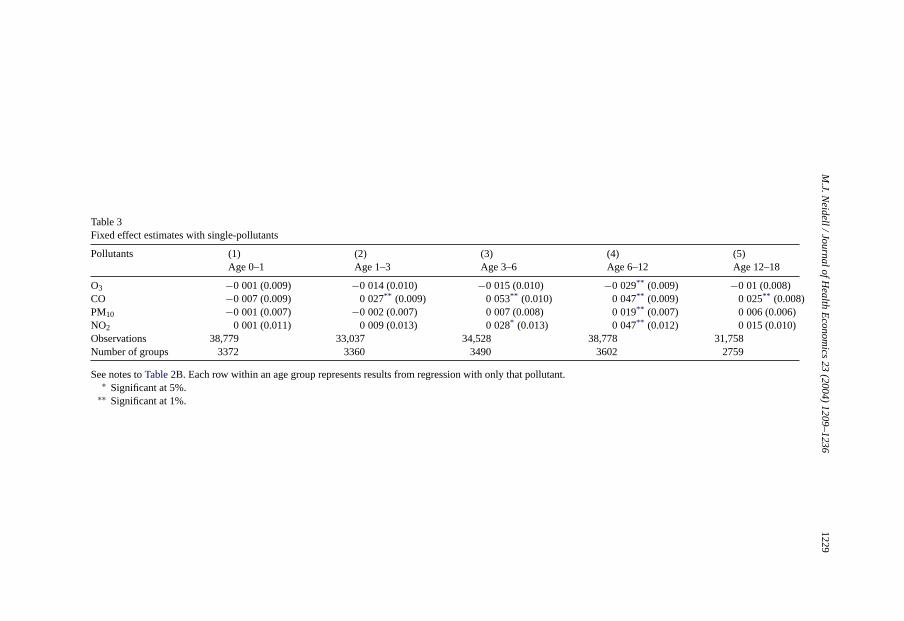
An additional concern with these estimates is that by controlling for pollutants simul-taneously it may be difficult to separately identify the effects of each pollutant. For ex-ample, as mentioned in the data section, NO2, CO, and PM10 are highly correlated pol-lutants.Table 3shows estimates from single-pollutant models. The effects of CO andNO2 are both larger in general. If automobile exhaust is truly a contributing factor toasthma, this finding is not surprising because automobile exhaust contributes heavily to bothpollutants.

An important issue to explore is whether the effect of pollution on asthma is the samefor all subsets of the population. Some groups, such as children with low health stock, mayface different risks from comparable levels of pollution. Additionally, asTable 1panel Bshows, pollution levels and asthma rates are higher for children of low SES. To assess theimportance of this, I interact each variable in Eq.(1) with an SES indicator as defined inTable 1panel B.33 These results, shown inTable 4, indicate that both O3 and CO have alarger effect on low SES children, with positive and significant effects on the interactionterm for ages 3–6 and 12–18. This supports the “double jeopardy” hypothesis that low SESchildren are not only exposed to higher levels of pollution but also are more harmed bysimilar amounts of pollution.

30 Since it is possible that the marginal effect of smog alerts varies with the number of smog alerts announced,I also estimated a model that included the square of smog alerts. This term was insignificant and did not affect theother estimates.

31 An alternative interpretation of these results is that smog alerts proxy for high levels of O3. This interpretationsuggests that O3 levels below 20 ppm have no effect on asthma admissions but levels above 20 ppm reduce thenumber of admissions, which is an unlikely scenario.

32 Additionally, including avoidance behavior controls specific to the other pollutants can increase the magnitudeof the coefficients for those pollutants.

33 I also performed this analysis by defining SES according to race and income, and the results were comparable.

M.J.N

eidell/Jo

urnalo

fHealth

Eco

nomics

23(2004)1209–1236

1229

Table 3Fixed effect estimates with single-pollutants

Pollutants (1) (2) (3) (4) (5)Age 0–1 Age 1–3 Age 3–6 Age 6–12 Age 12–18

O3 −0.001 (0.009) −0.014 (0.010) −0.015 (0.010) −0.029** (0.009) −0.01 (0.008)CO −0.007 (0.009) 0.027** (0.009) 0.053** (0.010) 0.047** (0.009) 0.025** (0.008)PM10 −0.001 (0.007) −0.002 (0.007) 0.007 (0.008) 0.019** (0.007) 0.006 (0.006)NO2 0.001 (0.011) 0.009 (0.013) 0.028* (0.013) 0.047** (0.012) 0.015 (0.010)Observations 38,779 33,037 34,528 38,778 31,758Number of groups 3372 3360 3490 3602 2759

See notes toTable 2B. Each row within an age group represents results from regression with only that pollutant.∗ Significant at 5%.

∗∗ Significant at 1%.

1230M.J.N

eidell/Jo

urnalo

fHealth

Eco

nomics

23(2004)1209–1236

Table 4Fixed effect estimates by age group and SES


O3 −0.007 (0.013) −0.003 (0.015) −0.038** (0.014) −0.044** (0.013) −0.022 (0.011)CO −0.017 (0.013) 0.000 (0.014) −0.016 (0.014) 0.000 (0.014) −0.003 (0.012)PM10 −0.006 (0.010) −0.012 (0.011) 0.004 (0.011) 0.011 (0.010) 0.005 (0.009)NO2 0.021 (0.017) −0.001 (0.020) 0.020 (0.020) 0.040* * �012 (0.011) T2()�


5.2. Magnitude of findings

To get a sense of the magnitude of these findings, I measure the percentage change (δ98)in asthma admissions in 1998 that has resulted from changes in pollution levels over time:

δ98 = E(Y |P92, A, X) − E(Y |P98, A, X)

E(Y |P98, A, X)(3)

whereE(Y|P92, A, X) is the expected number of asthma admission with 1992 levels ofpollution andE(Y|P98,A,X) is the expected number of asthma admissions with 1998 levelsof pollution. In other words,δ98 tells us how many asthma admissions in 1998 were avoidedbecause pollution levels were no longer at their 1992 levels. Using equation (1), we canrewrite (3) as:

δ98 = β0 · (P92 − P98)

E(Y |P98, A, X)(4)

whereβ0 is the coefficient of the effect of pollution on admissions. By treating the aboveestimates as causal, replacingβ0 with its estimated coefficient will provide an estimate ofδ98. Table 5A shows the declines in pollution since 1992 have decreased asthma admissionsin 1998 for children over 1 from 4.6 to 13.5%, with no effect for infants.

To get a rough idea of some of the annual economic benefits associated with these lowerlevels of pollution, I multiply the number of asthma hospitalizations in 1998 byδt to get an

Table 5Magnitude of estimates

A. Effect of change in pollution from 1992 to 1998 on asthma admissions in 1998

Age (years) δ98 (%) Average charge ($) Number of admissions Cost(δ98) ($)

0–1 −0.7 6819 1899 −84,9141–3 4.6 5915 1528 419,3023–6 13.5 6608 1865 1,666,2386–12 12.3 8272 2556 2,603,97412–18 6.6 9207 1017 619,774Total 5,224,372

B. Effect of SES and smog alerts on ER asthma admissions

Age (years) δa (%) δs (%)

0–1 −0.07 −0.691–3 −0.71 1.043–6 −0.45 5.906–12 −0.41 0.9212–18 −0.05 0.15

Notes: δ98 is the percentage change in ER admissions for asthma in 1998 only if pollution levels were at their1992 levels. Cost(δ98) = average charge x number of admissions× δ98. Coefficient estimates used to obtainδ98

are fromTable 2B. δa is the percentage change in ER admissions for asthma from the announcement of a smogalert. Coefficient estimates used to obtainδa are fromTable 2B. δs is the percentage change in ER admissions forasthma from higher pollution levels in low SES areas. Low SES is defined as zip code percentage of high schooldropouts less than median. Coefficient estimates used to obtainδs are fromTable 4.


estimate of the change in the number of asthma cases. Then I multiple this by the averagecost of hospitalization for asthma in 1998. Thus, the fall in pollution levels from thoseexperienced in 1992 has saved approximately $5.2 million in ER admissions for asthmain California in 1998 alone. These numbers, however, represent a lower bound of the truesocial benefits associated with reductions in asthma attacks. They only include emergencyroom admissions and their expenses in California, thus ignoring the rest of the U.S., othersources of care for asthma attacks, follow-up treatment, lost wages for the family, losthuman capital development of the child, psychic costs to the family, and any long-term linkto health problems for the child.34

Since avoidance behavior as measured by smog alerts has a significant effect on hos-pitalizations for asthma, it is useful to approximate the magnitude of these advisories. Tomeasure the percent reduction from an additional advisory conditional on O3 exceeding20 ppm, specify Eq.(4) as:

δa = β1

E(Y |P98, A = 1, X). (5)

Shown inTable 5B, replacingβ1 with its estimated coefficient, the announcement of asmog alert reduces asthma hospitalizations by 0.5–0.75% for children ages 1–12, but withno effect for the youngest and oldest children.

To get a sense of the magnitude of the SES findings, I estimate how much of the SESgap in asthma rates can be explained by pollution. To do this, I instead specify Eq.(4) as:

δs = β0s(PsS)

E(Y |Ps, S, A, X)(6)

whereβ0s is the coefficient on the pollution-SES interaction variables andS is an SESdummy variable.

These effects, shown inTable 5B, indicate that higher levels of pollution explain nearly6% of the difference in asthma ER admissions for ages 3–6, but little effect for other ages.35

This suggests that although the increased presence of pollution in low SES areas puts thesechildren at a higher risk for hospitalization from an asthma attack, there are still many otherfactors that affect this gap.

6. Discussion

There are three main findings in this paper. First, CO increases asthma hospitalizationsfor children ages 1–18. There does not appear to be much of an effect of these pollutantson infants, so looking at a broader range of outcomes can offer additional insights. Thepossibility of an effect for other pollutants, however, cannot be ruled out because these

34 SeeHarrington and Portney (1997)for a more detailed description of these additional costs. Unfortunately,there are no readily comparable measures of the costs to industry from increased pollution. SeeGreenstone (2002)for an excellent and up-to-date study of this subject.

35 This does not necessarily imply that pollution is more likely to induce asthma in low SES children. High SESchildren could use sources of care other than the hospital.


estimates are likely to represent lower bound estimates of the biological effect of pollutionon health. Furthermore, effects from shorter-term exposure to pollutants may go undetectedin a monthly analysis if there are threshold or other non-linear effects. Nevertheless, theseestimates are large in magnitude and suggest that the declines in pollution that have occurredover the 90s have greatly benefited children.

Second, avoidance behavior appears to play a significant role in reducing the effectof pollution on childhood asthma, as indicated by the negative effect of smog alerts onadmissions. While I am only able to control for one source of avoidance behavior that relatesonly to O3, it is possible that there are other unmeasured sources of avoidance behaviorthat may affect the other estimates. Given these findings, it is important to understand theeffects of other potential sources for avoidance behavior, as it can suggest other policies toimprove health outcomes. Moreover, the costs associated with avoidance behavior cannotbe ignored in a welfare analysis.

A third finding is that the net effect of pollution appears to be larger for children of lowerSES, suggesting that pollution may be responsible for some of the gradient in incidence ofasthma by SES. Furthermore, neurobiological and economic research has suggested thatearly shocks to a child’s health can persist for many years (Shonkoff and Marshall, 1990;Case et al., 2002; Currie and Hyson, 1999), and asthma itself has been associated with laterhealth conditions, including lung cancer (Ernster, 1996). Therefore, if poorer families areunable to afford to live in cleaner areas and as a result their children’s health developmentsuffers, this would suggest that pollution is one potential mechanism by which SES affectshealth.

Since current pollution standards are based on adult health responses, understanding thelink between pollution and children’s health has become increasingly important to a wideaudience, and particularly to the EPA. The next step in this project is to look at the linksbetween air pollution and other health outcomes, such as the incidence of low birth weightand other respiratory illnesses. The empirical strategy developed here appears to be fruitfulfor finding these links and developing more comprehensive measures of some of the healthbenefits from improvements in air quality.

Acknowledgement

I thank Janet Currie, Trudy Cameron, Paul Devereux, Joe Hotz, Ken Chay, MichaelGreenstone, J.R. DeShazo, Steven Haider, Wes Hartmann, and seminar participants at UC-Berkeley, UCLA, University of Miami, BLS, Census, EPA and RAND for many helpfulsuggestions. I am also particularly grateful to Bo Cutter for initiating my interest in this topicand to Resource for the Future for graciously providing funding via the Fisher DissertationAward.

Appendix A

SeeTables A.1–A.3.

1234M.J.N

eidell/Jo

urnalo

fHealth

Eco

nomics

23(2004)1209–1236

Table A.1Pollution correlation by distance, moitor sampling, and actual vs. estimated levels

A. Distance measure B. Monitor sampling C. Actual vs. estimated pollution levels

10 milesa 5 milesa # of monitors operating Correlationb Observations Monitors Correlationc

In 1992 In 1998 Continuously

O3 0.989 0.980 171 178 138 0.996 3141 106 0.925CO 0.974 0.952 91 88 75 0.989 1524 53 0.785PM10 0.981 0.983 125 149 98 0.981 1718 57 0.765NO2 0.986 0.974 109 108 87 0.993 2035 71 0.901

a These values represent correlations between estimated zip code pollution values using monitors within 20 miles from the zip code centroid and 10/5 miles.b These values represent the correlation between estimated zip code pollution values using any monitor in existence over the period 1992-1998 and onlycontinuously

operated monitors.c These values reprssent the correlation between actual and estimated pollution levels at each monitor. Pollution levels are estimated at each monitor using an

inverse-distance weighted average of all monitors within 20 miles.


Table A.2Pollution correlation matrix

O3 CO PM10 NO2

O3 1CO −0.4172 1PM10 0.3308 0.3901 1NO2 0.0469 0.7709 0.6513 1

Table A.3Characteristics of zip codes inside and outside 20 miles from monitors for all pollutants

>20 miles ≤20 miles |t|Median HH income 29,075 39,711 15.00% Urban 19% 87% 37.59% White 84% 71% 13.66% Black 2.0% 7.6% 11.20% <HS degree 26% 22% 4.15% College degree 16% 26% 13.38Total population <18 1,646,148 6,933,567 28.72Average ER asthma rate 0.134 0.102 2.96

References

Air Resources Board, 13 September 1990. Air Resources Board Sets New Warning Level for Urban Smog.California Environmental Protection Agency News Release.

American Academy of Pediatrics, 2000. Guide to Your Child’s Allergies and Asthma. Villard Books, New York.American Lung Association, as of 8/2001. Asthma.http://www.lungusa.org/asthma/index.html.Alberini, A., Krupnick, A., 1998. Air quality and episodes of acute respiratory illness in taiwan cities: evidence

from survey data. Journal of Urban Economics 44, 68–92.Bjorksten, B., 1999. The Environmental influence on childhood asthma. Allergy 54, 17–23.Bresnahan, B., Dickie, M., Gerking, S., 1997. Averting behavior and urban air pollution. Land Economics 73,

340–357.Case, A., Lubotsky, D., Paxson, C., 2002. Economic status and health in childhood: the origins of the gradient.

American Economic Review 92, 1308–1334.Chay, K., Greenstone, M., 2000. Does Air Quality Matter? Evidence from the Housing Market. Mimeograph.Chay, K., Greenstone, M., 2003. The impact of air pollution on infant mortality: evidence from geographic variation

in pollution shocks induced by a recession. Quarterly Journal of Economics (in press).Committee on the Medical Effects of Air Pollution, 2000. Asthma and Outdoor Air Pollution.

http://www.doh.gov.uk/comeap/airpol2.htm.Currie, J., Hyson, R., 1999. Is the impact of health shocks cushioned by socio-economic status? the case of low

birthweight. American Economic Review 89, 245–250.Desqueyroux, H., Momas, I., 1999. Air Pollution and health: analysis of epidemiological panel investigations

published from 1987 to 1998. Revue D Epidemiologie Et De Sante Publique 47, 361–375.Duhme, H., Weiland, S., Keil, U., 1998. Epidemiological analyses of the relationship between environmental

pollution and asthma. Toxicology Letters 102, 307–316.Eggleston, P., Buckley, T., Breysse, P., Wills-Karp, M., Kleeberger, S., Jaakkola, J., 1999. The environment and

asthma in U.S. inner cities. Environmental Health Perspectives 107, 439–450.Ernster, V., 1996. Female lung cancer. Annual Review of Public Health 17, 97–114.Fauroux, B., Sampil, M., Quenel, P., Lemoullec, Y., 2000. Ozone: a trigger for hospital pediatric asthma emergency

room visits. Pediatric Pulmonology 30, 41–46.

http://www.lungusa.org/asthma/index.html

http://www.doh.gov.uk/comeap/airpol2.htm


Friedman, M., Powell, K., Hutwagner, L., Graham, L., Teague, W., 2001. Impact of changes in transportation andcommuting behaviors during the 1996 summer olympic games in atlanta on air quality and childhood asthma.Journal of American Medical Association 285, 897–905.

Garty, B., Kosman, E., Ganor, E., Berger, V., Garty, L., Wietzen, T., Wasiman, Y., Mimouni, W., Waisel, Y., 1998.Emergency room visits of asthmatic children, relation to air pollution, weather, and airborne allergens. Annalsof Allergy Asthma and Immunology 81, 563–570.

Gouveia, N., Fletcher, T., 2000. Respiratory diseases in children and outdoor air pollution in Sao Paulo Brazil: atime series analysis. Occupational and Environmental Medicine 57, 477–483.

Greenstone, M., 2002. The Impacts of environmental regulations on industrial activity: evidence from the 1970and 1977 Clean air act amendments and the census of manufacturers. Journal of Political Economy 110,1175–1219.

Harrington, W., Portney, P., 1997. Valuing the benefits of health and safety regulation. Journal of Urban Economics22, 101–112.

Krupnick, A., Harrington, W., Ostro, B., 1990. Ambient ozone and acute health effects: evidence from daily data.Journal of Environmental Economics and Management. 17, 1–18.

Letourneau, M., Schum, S., Gausche, M., 1992. Respiratory disorders. In: Barkin, R. (Ed.), Pediatric EmergencyMedicine: Concepts and Clinical Practice. Mosby-Year Book Inc., St. Louis.

Managed Risk Medical Insurance Board, 8/2001. AIM Fact Book 1998.http://www.mrmib.ca.gov/.National Institute of Environmental Health Sciences, 1/2000. Asthma and Allergy Prevention.http://www.

niehs.nih.gov/airborne/research/background.html.Norris, G., YoungPong, S., Koenig, J., Larson, T., Sheppard, L., Stout, J., 1999. An association between fine

particles and asthma emergency department visits for children in Seattle. Environmental Health Perspectives107, 489–493.

Nystad, W., 2000. Asthma. International Journal of Sports Medicine 21, 98–102.Nystrom, M., 8/2001. California Air Quality Status and Trends 1999. Presentation to California Air Resources

Board,http://www.arb.ca.gov/aqd/aqtrends/trends1.htm.Portney, P., Mullahy, J., 1986. Urban air quality and acute respiratory illness. Journal of Urban Economics 20,

21–38.Portney, P., Mullahy, J., 1990. Urban air quality and chronic respiratory disease. Regional Science and Urban

Economics 20, 407–418.Ransom, M., Pope III, C.A., 1995. External health costs of a steel mill. Contemporary Economic Policy 13, 86–97.Seaton, A., et al., 1995. Particulate air pollution and acute health effects. The Lancet 354, 176–178.Shonkoff, J., Marshall, P., 1990. Biological Bases of Developmental Dysfunction. In: Meisels, S., Shonkoff, J.

(Eds.), Handbook of Early Childhood Intervention. Cambridge University Press, Cambridge, MA.Speizer, F., 2001. Childhood Asthma. Presentation at Health Effect Institute Annual Conference, Air Pollution

and Populations at Risk, Washington, DC.United States Environmental Protection Agency, 1999. Guidelines for Reporting of Daily Air Quality - Air Quality

Index (AQI). EPA Document #454-R-99-010, Research Triangle Park, NC.United States Environmental Protection Agency, 1999b. Conceptual Strategies for Ambient Air Monitoring. Draft

version 2.United States Environmental Protection Agency, 2000. Air Quality Criteria for Carbon Monoxide. EPA Document

# 600-P-99-001F, Washington, DC.United States Environmental Protection Agency, 2003. Criteria Pollutants,http://www.epa.gov/oar/oaqps/

greenbk/o3co.html.Vacek, L., 1999. Is the Level of Pollutants a Risk Factor for Exercise-induced Asthma Prevalence? In: Allergy and

Asthma Proceedings vol. 20., pp. 87–93.von Mutius, E., 2000a. Can Natural History of Asthma Be Modified? Revue Francaise D Allergologie Et D

Immunologie Clinique. 40, 689–694.von Mutius, E., 2000b. The Environmental Predictors of Allergic Disease. Journal of Allergy and Clinical Im-

munology. 105, 9–19.Wilson, R., Spengler, J., 1996. Particles in Our Air: Concentration and Health Effects.. Harvard University Press,

Cambridge, MA.Zeckhauser, R., Fisher, A., 1976. Averting Behavior and External Diseconomies. Kennedy School Discussion

Paper 41D.

http://www.mrmib.ca.gov/

http://www.niehs.nih.gov/airborne/research/background.html

http://www.niehs.nih.gov/airborne/research/background.html

http://www.arb.ca.gov/aqd/aqtrends/trends1.htm

http://www.epa.gov/oar/oaqps/greenbk/o3co.html

http://www.epa.gov/oar/oaqps/greenbk/o3co.html

air pollution, health, and socio-economic status: the

Documents