air-mist spray model development in steel secondary
TRANSCRIPT

AIR-MIST SPRAY MODEL DEVELOPMENT IN STEEL SECONDARY
COOLING PROCESS
by
Edwin Andres Mosquera Salazar
A Thesis
Submitted to the Faculty of Purdue University
In Partial Fulfillment of the Requirements for the degree of
Master of Science in Mechanical Engineering
Department of Mechanical and Civil Engineering
Hammond, Indiana
May 2020
2
THE PURDUE UNIVERSITY GRADUATE SCHOOL
STATEMENT OF COMMITTEE APPROVAL
Dr. Chenn Q. Zhou, Chair
Department of Mechanical and Civil Engineering
Dr. Nesrin Ozalp
Department of Mechanical and Civil Engineering
Dr. Ran Zhou
Department of Mechanical and Civil Engineering
Approved by:
Dr. Chenn Q. Zhou Head of the Graduate Program

3
To Family, the ones who will always believe and love me

4
ACKNOWLEDGMENTS
I would like to thank the Steel Manufacturing Simulation and Visualization Consortium
(SMSVC) for funding this project. The Center for Innovation through Visualization and
Simulation (CIVS) at Purdue University Northwest is also gratefully acknowledged for
providing all the resources required for this work. Last but not least, I appreciate the help and
advice from Professor Chenn Zhou, Dr. Armin Silaen, and Haibo Ma, all great role models.

5
TABLE OF CONTENTS
TABLE OF CONTENTS ................................................................................................................ 5
LIST OF TABLES .......................................................................................................................... 8
LIST OF FIGURES ........................................................................................................................ 9
ABSTRACT .................................................................................................................................. 11
INTRODUCTION .............................................................................................. 12 CHAPTER 1.
1.1 Literature Review.............................................................................................................. 13
1.1.1 Single-phase and two-phase nozzles ......................................................................... 13
1.1.2 Spray characterization of nozzles and heat transfer .................................................. 14
1.1.3 Atomization ............................................................................................................... 15
1.1.4 VOF-to-DPM model .................................................................................................. 15
1.1.5 Mesh refinement adaptation methods ........................................................................ 16
1.1.6 Mesh types ................................................................................................................. 17
1.1.7 Turbulence models ..................................................................................................... 17
1.2 Objectives ......................................................................................................................... 18
METHODOLOGY AND CFD MODELS .......................................................... 19 CHAPTER 2.
2.1 Methodology ..................................................................................................................... 19
2.1.1 Cross-flow simulation ................................................................................................ 19
2.1.2 Air-mist nozzle simulation ........................................................................................ 20
2.2 CFD Models ...................................................................................................................... 22
2.2.1 Conservation of mass ................................................................................................. 22
2.2.2 Momentum equation .................................................................................................. 22
2.2.3 VOF model ................................................................................................................ 22
2.2.3.1 Implicit scheme ..................................................................................................... 23
2.2.3.2 Explicit scheme ..................................................................................................... 23
2.2.4 Lagrangian model DPM ............................................................................................ 23
2.2.5 Breakup model ........................................................................................................... 23
2.2.6 Nukiyama-Tanasawa distribution equation ............................................................... 25
2.2.7 Turbulence models ..................................................................................................... 25
2.2.7.1 Realizable k-epsilon ............................................................................................. 25

6
2.2.7.2 SST k-omega ........................................................................................................ 26
2.2.7.3 Large Eddy Simulation (LES) .............................................................................. 27
2.2.7.4 Algebraic WMLES model .................................................................................... 27
CROSS-FLOW SIMULATION ......................................................................... 28 CHAPTER 3.
3.1 Computational Domain and Boundary conditions ............................................................ 28
3.2 Results and Analysis ......................................................................................................... 30
3.2.1 Effect of mesh adaptation methods ............................................................................ 30
3.2.2 Effect of turbulence models ....................................................................................... 33
3.2.3 Effect of mesh resolution ........................................................................................... 36
3.3 Validation .......................................................................................................................... 36
AIR-MIST NOZZLE SIMULATION ................................................................ 40 CHAPTER 4.
4.1 Nozzle internal region, Section 1 (VOF model) ............................................................... 40
4.1.1 Computational domain ............................................................................................... 40
4.1.2 Boundary conditions and fluid-gas properties ........................................................... 40
4.1.3 Effect of mesh types and mesh sensitivity study ....................................................... 41
4.1.4 Effect of operating conditions ................................................................................... 44
4.1.5 Quasi-steady state of simulation cases ...................................................................... 46
4.2 Spray formation region, Section 2 .................................................................................... 47
4.2.1 Computational domain and boundary conditions ...................................................... 47
4.2.2 Spray characterization (VOF model) ......................................................................... 50
4.2.3 Droplet generation methods ....................................................................................... 52
4.2.3.1 VOF-to-DPM model ............................................................................................. 52
4.2.3.2 Nukiyama-Tanasawa distribution equation model (DPM model) ........................ 53
4.3 Validation .......................................................................................................................... 54
AIR-MIST NOZZLES COMPARISON ............................................................. 57 CHAPTER 5.
5.1 Nozzle internal region, Section 1 (VOF model) ............................................................... 57
5.1.1 Computational domain and boundary conditions ...................................................... 57
5.1.2 Mesh sensitivity study ............................................................................................... 57
5.1.3 Air-mist nozzles comparison ..................................................................................... 59
5.1.4 Quasi-steady state of simulation cases ...................................................................... 60
5.2 Spray characterization between nozzles, Section 2 (VOF model) .................................... 61

7
CONCLUSIONS ................................................................................................. 64 CHAPTER 6.
6.1 Cross-flow simulation ....................................................................................................... 64
6.2 Air-mist nozzle simulation ................................................................................................ 64
REFERENCES ............................................................................................................................. 65
APPENDIX A. MATLAB CODE FOR INTERPOLATION FLUID-GAS PROPERTIES ........ 68
APPENDIX B. RATIO APPROXIMATION TO FIND LIMITS IN CUMULATIVE VOLUME
SIZE DISTRIBUTION ................................................................................................................. 75
PUBLICATIONS .......................................................................................................................... 77

8
LIST OF TABLES
Table 1. Droplet size terminology [5] . ......................................................................................... 14
Table 2. Turbulence models in Fluent. ......................................................................................... 18
Table 3. Fluid properties and boundary conditions of fluid and air phases. ................................. 30
Table 4. Mesh resolution and total droplet generated. .................................................................. 36
Table 5. Boundary conditions for simulation cases. ..................................................................... 41
Table 6. Polyhedral mesh sensitivity study................................................................................... 43
Table 7. Conditions at the nozzle tip. ........................................................................................... 46
Table 8. Relations of operating conditions and velocity of the air-mist nozzle. .......................... 51
Table 9. Comparison measurement and CFD continuous at monitor location ............................. 52
Table 10. Performance of droplet generation methods. ................................................................ 55
Table 11. Validation for droplet size distribution. ........................................................................ 56
Table 12. Polyhedral mesh sensitivity study................................................................................. 58
Table 13. Conditions at the nozzle tip. ......................................................................................... 60

9
LIST OF FIGURES
Figure 1. Schematic of continuous caster [1] . .............................................................................. 12
Figure 2. VOF-to-DPM transition model...................................................................................... 20
Figure 3. Air-mist spray model. .................................................................................................... 21
Figure 4. Droplet generation methodology. .................................................................................. 21
Figure 5. Cross-flow domain. ....................................................................................................... 28
Figure 6. (a) Testing mesh, (b) Validation mesh. ......................................................................... 29
Figure 7. (a) PUMA mesh adaptation, (b) VOF-to-DPM transition using WMLES S-Omega. ... 31
Figure 8. (a) Hanging Node Adaptation, (b) VOF-to-DPM transition using WMLES S-Omega. 32
Figure 9. Effect of mesh adaptation methods in droplet size distribution on plane 1. ................. 32
Figure 10. (a) Velocity and liquid volume fraction, (b) VOF-to-DPM transition using WMLES
S-Omega. ...................................................................................................................................... 33
Figure 11. (a) Velocity and liquid volume fraction, (b) VOF-to-DPM transition using Realizable
k-epsilon. ....................................................................................................................................... 34
Figure 12. (a) Velocity and liquid volume fraction, (b) VOF-to-DPM using SST k-omega. ....... 35
Figure 13. Effect of turbulence models in droplet size distribution on plane 1. ........................... 35
Figure 14. PUMA mesh adaptation on XY cross-section midplane. ............................................ 37
Figure 15. Velocity magnitude and liquid VOF. .......................................................................... 37
Figure 16. VOF-to-DPM transition............................................................................................... 38
Figure 17. Validation for droplets size distribution. ..................................................................... 39
Figure 18. Section 1, Delavan Cool-Cast air-mist nozzle 3D geometry. ...................................... 40
Figure 19. Tetrahedral mesh using ANSYS, (b) Polyhedral mesh using STAR-CCM+. ............. 42
Figure 20. (a) Internal reference line (b) Velocity along the reference line for all surface
remesher proximity factors. .......................................................................................................... 43
Figure 21. Absolute pressure along the reference line. ................................................................. 44
Figure 22. Velocity magnitude along the reference line. .............................................................. 45
Figure 23. Water concentration VOF along the reference line. .................................................... 45
Figure 24. Monitor point. .............................................................................................................. 46
Figure 25. The convergence of the probe point at 20,000 iterations. ........................................... 47
Figure 26. Section 2, spray region. ............................................................................................... 47

10
Figure 27. Polyhedral mesh, potential core area refined (500μm)................................................ 48
Figure 28. (a) Potential core area refined (100μm), (b) Top view injection imprinted face......... 49
Figure 29. (a) Hexahedral mesh, (b) top view injection imprinted face (1mm). .......................... 49
Figure 30. Air-mist nozzles spray characterization. ..................................................................... 50
Figure 31. CFD and test spray comparison. .................................................................................. 51
Figure 32. Normalized typical cumulative volume size distribution [5] . .................................... 53
Figure 33. Air-mist spray velocity magnitude. ............................................................................. 54
Figure 34. Comparison of droplet generation methods. ............................................................... 55
Figure 35. Cumulative volume size distribution for both methods. ............................................. 56
Figure 36. Section 1, Spraying System Caster-Jet 3D model. ...................................................... 57
Figure 37. (a) Internal reference line, (b) Velocity along the reference line for all surface
remesher proximity factors. .......................................................................................................... 58
Figure 38. Absolute pressure along the reference line. ................................................................. 59
Figure 39. Velocity magnitude along the reference line. .............................................................. 59
Figure 40. Water concentration VOF along the reference line. .................................................... 60
Figure 41. Monitor points. ............................................................................................................ 61
Figure 42. The convergence of the probe point at 20,000 iterations. ........................................... 61
Figure 43. Air-mist nozzles spray characterization. ..................................................................... 62
Figure 44. Spray coverage at 190mm standoff distance. .............................................................. 63

11
ABSTRACT
Continuous casting is an important process to transform molten metal into solid. Arrays of spray
nozzles are used along the process to remove heat from the slab letting it solidify. Efficient and
uniform heat removal without slab cracking is desired during steel continuous casting, and air-
mist sprays could help to achieve this goal. Air-mist nozzles are one of the important keys for
determining the quality of steel as well as energy consumption for pumping the water. Based on
industrial data, it is estimated that a 1% reduction in scrapped production due to casting related
defects can result in annual savings of 40.53 million dollars in the U.S. Computational
simulations studies can minimize defects in steel such as cracks, inclusions, macro-segregations,
porosity, and others, which are closely related to the heat transfer between water droplets and hot
slab surface.
Conducting multiple spray experiments in order to find optimum operating conditions might be
impractical and expensive in some cases. Thus, Computational Fluid Dynamics (CFD)
simulation is aimed to be used for simulating the air-mist spray process. Because it is a
challenging process due to strong air and water interaction, then numerical models have been
developed to simulate water droplets. The first model involves air and water phases which then
are transformed in single-phase water droplets. To do so, a Volume of Fraction (VOF) to the
Discrete Phase Model (DPM) is used.
VOF-TO-DPM transition model involves the primary and secondary breakup which occurs in the
water atomization process, starting with a single water core, followed by a smaller compact
mass of water known as lumps or ligaments due to the interaction of air, and finally converted
into water droplets. The second model is using the Nukiyama-Tanasawa function size
distribution which injects water droplets based on defined size range and velocity profile. A
validation of droplet size and velocity against experimental data has been accomplished. The
models can avoid acquiring expensive equipment in order to understand nozzle spray
performance, and droplets generated. Quality, water droplet velocity, size, energy, and water
consumption are the core of the current study. Last but not least, the methodology for this model
can be used in any other air-mist nozzle design.

12
INTRODUCTION CHAPTER 1.
In the steel making, continuous casting is the process where molten steel is poured into a ladle,
tundish and mould, see Figure 1. This process allows producing continuously ingots, slabs,
blooms or billets [1] that will be later turned into structural parts, bars, rods, or coils. The casting
speed mainly changes depending on the steel composition. Arrays of spray nozzles cool down
the surface, removing heat as uniform as possible to avoid defective parts. The part is solidified
at the end of the process. This thesis study focuses on the secondary cooling section, developing
an air-mist nozzle model using CFD.
Figure 1. Schematic of continuous caster [1] .

13
1.1 Literature Review
1.1.1 Single-phase and two-phase nozzles
Under the same spray density conditions, single-phase e.g. hydraulic nozzle produces droplet
size of the order of thousand microns and two-phase e.g. air-mist nozzle produces droplet size of
the order of tens to hundreds of microns [2] . Smaller droplets can evaporate quicker, and it can
reduce the water build-up under rolls. Another advantage of using air-mist nozzles is the
innovative easy tip and tube replacement design, giving the chance to low downtime because of
nozzle clogging and breakouts [2] . There are different droplet tests to measure velocity, pressure,
uniformity, and size. For instance, impact test can be calculated using theoretical formulas
without considering the turbulence, conducting experiments is important to calculate impact
force, lateral distribution, and transverse distribution on the covered area that is being tested [2] .
A force transducer is used for scanning the impact pressure from droplets impinging a surface
[3] .
Delavan Cool-Cast W19917-15 is the flat fan air-mist nozzle used for this research. The spray
characterization for this nozzle was tested using a two-dimensional system Artium Technologies
Phase Doppler Interferometry (PDI)-300MD. Industrial collaborators conducted tests, and details
about the laser types and positions of the receiver and transmitter cannot be disclosed from the
experiment. Drop size and velocity measurements were obtained using these tests. Another test
to collect data is the Phase Doppler Particle Analyzer (PDPA) test which can go from agriculture
application to a natural disaster like a hurricane [4] . Droplet size terminology can be seen in
Table 1 [5] . Computational Fluid Dynamics (CFD) simulations can be also used to optimize the
spraying, collected experimental data is used as input for the simulation in order to improve the
accuracy, velocity, pressure, turbulence, flow patterns, and droplets trajectories, among others
variables, can be obtained from CFD analysis [2] .
14
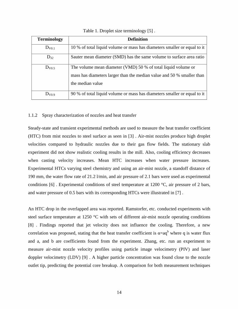
Table 1. Droplet size terminology [5] .
Terminology Definition
DV0.1 10 % of total liquid volume or mass has diameters smaller or equal to it
D32 Sauter mean diameter (SMD) has the same volume to surface area ratio
DV0.5 The volume mean diameter (VMD) 50 % of total liquid volume or
mass has diameters larger than the median value and 50 % smaller than
the median value
DV0.9 90 % of total liquid volume or mass has diameters smaller or equal to it
1.1.2 Spray characterization of nozzles and heat transfer
Steady-state and transient experimental methods are used to measure the heat transfer coefficient
(HTC) from mist nozzles to steel surface as seen in [3] . Air-mist nozzles produce high droplet
velocities compared to hydraulic nozzles due to their gas flow fields. The stationary slab
experiment did not show realistic cooling results in the mill. Also, cooling efficiency decreases
when casting velocity increases. Mean HTC increases when water pressure increases.
Experimental HTCs varying steel chemistry and using an air-mist nozzle, a standoff distance of
190 mm, the water flow rate of 21.2 l/min, and air pressure of 2.1 bars were used as experimental
conditions [6] . Experimental conditions of steel temperature at 1200 °C, air pressure of 2 bars,
and water pressure of 0.5 bars with its corresponding HTCs were illustrated in [7] .
An HTC drop in the overlapped area was reported. Ramstorfer, etc. conducted experiments with
steel surface temperature at 1250 °C with sets of different air-mist nozzle operating conditions
[8] . Findings reported that jet velocity does not influence the cooling. Therefore, a new
correlation was proposed, stating that the heat transfer coefficient is α=aqb where q is water flux
and a, and b are coefficients found from the experiment. Zhang, etc. run an experiment to
measure air-mist nozzle velocity profiles using particle image velocimetry (PIV) and laser
doppler velocimetry (LDV) [9] . A higher particle concentration was found close to the nozzle
outlet tip, predicting the potential core breakup. A comparison for both measurement techniques
15
was plot using air pressure of 0.2 MPa and water pressure of 0.4 MPa. Also, a velocity
distribution equation was proposed describing the entire flow field.
Cheng, etc. conducted Eulerian multiphase CFD simulations using a prototype nozzle [10] . The
boundary condition for air inlet was chosen as pressure inlet while water inlet as mass flow inlet.
Liquid fractions at nozzle outlet were found between 0.07 and 0.3; depending on the simulated
conditions. Moreover, increasing the air pressure, increases water droplets velocity, while
increasing the water pressure, decreases water droplets velocity. Vashahi, etc. simulated a CFD
case, using the VOF method where a pressure swirl nozzle with 8.7 million hex cells from the
internal and external nozzle was used in order to predict accurately the swirling flow [11] .
1.1.3 Atomization
Arthur, etc claims basic process that governs the development of emerging liquid stream, its
disintegration into ligaments and droplets. Also, spray characterization depends on the internal
geometry and physical properties of the liquid and gas medium [12] . Moreover, different
functions allow coming up with mathematical representations of measured droplet size
distribution; among them are normal, log-normal, Nukiyama-Tanasawa, Rosin-Rammler, and
upper limit distribution. Nukiyama-Tanasawa is a function that has four independent constants
that allow capturing multiple distributions compared to other functions that use two parameters
such as Rosin-Rammler [12] . STAR-CCM+ 13.04.010 has the Nukiyama-Tanasawa droplet size
generator model and this states that typical uses are in high speed liquid sprays in IC engines
[13] . Accurate distribution of droplet size is a very important parameter for analysis of mass and
heat transport [14] -- [15] . Also, researchers have used Nukiyama-Tanasawa concluding that
droplet size distribution showed good agreement with samples studied [14] -- [16] .
1.1.4 VOF-to-DPM model
Volume of Fluid (VOF) and Discrete Phase Model (DPM) has been tried to be coupled in the
past by other researchers. There are some disadvantages if models are run separately. For
example, simulating all length scales at once in a spray in a jet engine can be inefficient and
impractical if there is not a consideration of domain size and cell size of the order of microns
[17] . Also, a lower-cost strategy can be using DPM by tracking Lagrangian particles;

16
nevertheless, droplets can be adequately computed far from the solid-liquid core in the dispersed
region, but they cannot be captured accurately near the liquid core.
The hybridization of two models into a single spray modeling technique using an algorithm of
droplet identification based on Connected Components Labeling (CCL) was proposed in [17] .
Coupled Level Set and Volume of Fluid (CLSVOF) and the DPM Lagrangian tracking using
adaptive mesh refinement were simulated in [18] . Where neighbor search algorithms were used
on the finest refinement level in order to find candidates droplets for the DPM tracking from the
liquid-gas interfaces in the Eulerian domain. Furthermore, an extensive explanation of CPU time
based on mesh resolutions for validated cases were also reported. ANSYS FLUENT 19.1
illustrates in [19] the VOF-to-DPM transition criteria when the lumps are close to a spherical
shape, considering 0 as a perfect sphere for asphericity. A normalized standard deviation by the
average radius will be calculated between facets center on each lump with respect to its center of
gravity. Moreover, average radius-surface orthogonality will be calculated from the relative
orthogonality of every facet of the lump surface. A split factor definition is introduced in
ANSYS Fluent webinar [20] ; this input factor can either create more or fewer parcels if the
DPM parcel exceeds the cell volume.
1.1.5 Mesh refinement adaptation methods
Hanging Node Adaptation and Polyhedral Unstructured Mesh Adaptation (PUMA) are mesh
refinement adaptation methods. Hanging Node Adaptation and PUMA will refine or coarsen the
cell from the node that is not vertices of all sharing cells [21] . Also, the Hanging Node
Adaptation method consumes more memory in order to maintain the mesh hierarchy and store
temporary edges in 3D. In contrast, PUMA consumes less memory. Mesh cannot be coarsened
further than the original cell size for both methods. PUMA can refine all cell types while
Hanging Node Adaptation can refine all cell types but polyhedral. Gradient adaptation with
water volume fraction as the variable can set a coarsen threshold and a refine threshold. Values
above the refine threshold will be refined and values below coarsen one will be coarsened [22] .
This is applicable for both adaptive methods. Both methods can either use the first gradient or
second gradient; gradient or curvature respectively, depending if the simulated case involves a
strong shock or smooth solution.

17
1.1.6 Mesh types
Using structured or unstructured grids depends indirectly on the simulation case that is trying to
be accomplished, considering accuracy and efficiency. Polyhedral mesh is derived from
tetrahedral mesh according to [23] ; polygons will be formed around each node in the tetrahedral
mesh. Polyhedral mesh can also achieve faster converge solutions than Hexahedral and
Tetrahedral mesh, again depending of the case. Tetrahedral mesh contains approximately five
times more cells than a polyhedral mesh [23] -- [24] . Also, some meshing controls can be
changed when doing the mesh. For instance, a growth factor less than 1 will create a slower cell
growth, having more elements, leading a more dense mesh. Another control to increase the
number of faces and cells is surface remesher proximity where the value of number points in a
gap can be modified to create more or less faces, resulting in local refinements in the domain.
Quality can also be checked after the mesh is completed, showing the smoothness between cells.
Wake refinement allows the user to define a direction, distance, size and spread angle with
respect to a part surface where the refinement will take place.
1.1.7 Turbulence models
Table 2 shows the turbulence models and the increment in computational time [25] . Reynolds-
Averaged Navier Stokes (RANS) solve a time-averaged flow solution while Large Eddy
Simulation (LES) solves for larger eddies, and models for smaller eddies in the solution. Three
turbulence models were used for this research. Realizable k-ε is more robust compared to
Standard k-ε; it can be used when flows involve rotation, boundary layers, separation, and
recirculation. Wall functions can be used to resolve the turbulence near the wall after checking
the corresponding y+ which is the dimensionless wall distance. SST k-ω is a hybrid model which
combines outer layer (wake and outward) and inner layer (sub-layer, log-layer) into a blended
law of the wall. WMLES S-Omega is an enhance the subgrid-scale model to capture the LES
portion using the absolute difference of strain rate (S) and vorticity magnitude (Ω) [22] .

18
Table 2. Turbulence models in Fluent.
One-Equation Model
Spalart-Allmaras
Two-Equation Models
Standard k-ε
RNG k-ε
Realizable k-ε
RANS based
models
Standard k-ω
SST k-ω
Increase in
Computational
Cost
Per Iteration
4-Equation v2f*
Reynolds Stress Model
k-kl-ω Transition
Model
SST Transition Model
Detached Eddy
Simulation
Large Eddy Simulation
1.2 Objectives
Current work for numerical simulation focuses on the development of an air-mist spray model.
Proposing a three-step methodology to simulate the actual air-mist spray. Evaluating two
approaches to generate droplets using either the VOF-to-DPM transition model or the Nukiyama-
Tanasawa distribution function. Also, validation of droplet size and droplet velocity magnitude
against literature and experiment are included in this research.

19
METHODOLOGY AND CFD MODELS CHAPTER 2.
Hydraulic nozzles and air-mist nozzles are used in steel continuous casters during the secondary
cooling region. This research emphasizes air-mist nozzles because of the advantages stated in
CHAPTER 1. It has not been published a full methodology to simulate air-mist nozzles. To do
so, a cross-flow example has been used as a foundation simulation to test the VOF-to-DPM
transition model, the effects of turbulence models, mesh adaptation methods, and mesh
resolution. Then, the transition model and Nukiyama-Tanasawa distribution function have been
implemented in simulating a flat fan Cool-Cast W19917-15 air-mist nozzle that has been used in
the industry. This methodology is currently being applied to a second flat fan Spraying System
Caster-Jet 50070 air-mist nozzle.
2.1 Methodology
2.1.1 Cross-flow simulation
A cross-flow example adopted from the work by Xiaoyi et al. [18] was used as a benchmark
simulation to test the VOF-to-DPM transition model. The cross-flow simulation involves liquid
and air phases, taking care by the VOF model. Because of the presence of the air stream, the
liquid atomization process breakup can occur. Figure 2 illustrates simply how this model works.
This model is activated from VOF-to-DPM when a liquid lump or ligament has a shape close to
a sphere and size based on given user input. When these occur a liquid lump will take a spherical
shape using the DPM model and its liquid phase in the cell in the continuous domain will be
replaced by the second phase that is air. If mesh adaptive is used to help to achieve droplets
certain size, then after the transition the cell can be coarsened back to reduce computation effort.

20
Figure 2. VOF-to-DPM transition model.
2.1.2 Air-mist nozzle simulation
Figure 3 shows the methodology to simulate an air mist nozzle being separated into three
independent but linked sections. It was considered that way because of computational time,
seeing the sections as a complete spray process. Section 1 uses the VOF method because of the
presence of air gas and water liquid phases interacting inside the air-mist nozzle. When
numerical solution achieves quasi-steady state, gas-liquid distribution and velocities components
will be used as an injection profile at a fixed reference location near the nozzle tip leading the
analysis to section 2. Thus, spraying going through the primary and secondary breakup will
occur where the VOF-to-DPM transition model will be used. DPM model will be used in section
3 to continue the spray simulation using droplets size distribution and velocities components.
Water droplets will eventually impinge a hot slab surface in order to remove heat; however, this
research neglect the heat transfer analysis and focuses on simulating air-mist nozzle spray
development.

21
Figure 3. Air-mist spray model.
The VOF-to-DPM transition model is able to convert the liquid phase into liquid droplet. A
second option to generate droplets can be using distribution equations, in this research
Nukiyama-Tanasawa will be used, see Figure 4.
Figure 4. Droplet generation methodology.

22
2.2 CFD Models
Three-dimensional numerical simulations for both cross-flow and air-mist nozzle have been
developed using the following equations and models. Mass and heat transfer between slab and
liquid droplet has been neglected for current work.
2.2.1 Conservation of mass
𝐷ρ
𝐷𝑡+ 𝜌∇ ∗ �⃗� = 0 (1)
2.2.2 Momentum equation
Velocity will be shared between phases. However, accuracy near the phase’s interface can be
affected with larger velocity differences bringing into consideration to select the appropriate
interface capturing scheme.
∂
∂t(ρ�⃗�) + ∇ ∗ (ρ�⃗��⃗�) = −∇p + ∇ ∗ [μ(∇�⃗� + ∇�⃗�T)] + ρ�⃗� + �⃗� (2)
2.2.3 VOF model
Tracking phases is accomplished after solving the continuity equation for the volume fraction of
phases.
1
𝜌𝑞[
∂
∂t(αq𝜌𝑞) + ∇(αq𝜌𝑞𝑣𝑞⃗⃗⃗⃗⃗) = ∑ (𝑚𝑝𝑞̇ − 𝑚𝑞𝑝̇ )𝑛
𝑝=1 ] (3)
Where the mass transfer from phase q to phase p is 𝑚𝑞𝑝̇ , and mass transfer from phase p to phase
q is 𝑚𝑝𝑞̇ . Volume fraction can be solved using implicit or explicit discretization in order to solve
face fluxes between cells.
23
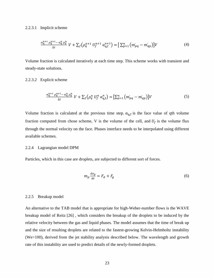
2.2.3.1 Implicit scheme
αq𝑛+1 𝜌𝑞
𝑛+1− αq𝑛 𝜌𝑞
𝑛
∆𝑡 𝑉 + ∑ (𝜌𝑞
𝑛+1 𝑈𝑓𝑛+1 αq,f
𝑛+1) =𝑓 [ ∑ (𝑚𝑝𝑞̇ − 𝑚𝑞𝑝̇ )𝑛𝑝=1 ]𝑉 (4)
Volume fraction is calculated iteratively at each time step. This scheme works with transient and
steady-state solutions.
2.2.3.2 Explicit scheme
αq𝑛+1 𝜌𝑞
𝑛+1− αq𝑛 𝜌𝑞
𝑛
∆𝑡 𝑉 + ∑ (𝜌𝑞
𝑛 𝑈𝑓𝑛 αq,f
𝑛 ) =𝑓 [∑ (𝑚𝑝𝑞̇ − 𝑚𝑞𝑝̇ )𝑛𝑝=1 ]𝑉 (5)
Volume fraction is calculated at the previous time step. αq,f is the face value of qth volume
fraction computed from chose scheme, V is the volume of the cell, and 𝑈𝑓 is the volume flux
through the normal velocity on the face. Phases interface needs to be interpolated using different
available schemes.
2.2.4 Lagrangian model DPM
Particles, which in this case are droplets, are subjected to different sort of forces.
𝑚𝑝𝑑𝑣𝑝
𝑑𝑡= 𝐹𝑑 + 𝐹𝑔 (6)
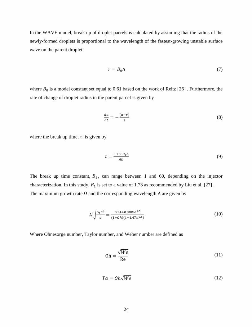
2.2.5 Breakup model
An alternative to the TAB model that is appropriate for high-Weber-number flows is the WAVE
breakup model of Reitz [26] , which considers the breakup of the droplets to be induced by the
relative velocity between the gas and liquid phases. The model assumes that the time of break up
and the size of resulting droplets are related to the fastest-growing Kelvin-Helmholtz instability
(We>100), derived from the jet stability analysis described below. The wavelength and growth
rate of this instability are used to predict details of the newly-formed droplets.
24
In the WAVE model, break up of droplet parcels is calculated by assuming that the radius of the
newly-formed droplets is proportional to the wavelength of the fastest-growing unstable surface
wave on the parent droplet:
𝑟 = 𝐵0Λ (7)
where 𝐵0 is a model constant set equal to 0.61 based on the work of Reitz [26] . Furthermore, the
rate of change of droplet radius in the parent parcel is given by
𝑑𝑎
𝑑𝑡= −
(𝑎−𝑟)
𝜏 (8)
where the break up time, 𝜏, is given by
𝜏 =3.726𝐵1𝑎
𝛬𝛺 (9)
The break up time constant, 𝐵1 , can range between 1 and 60, depending on the injector
characterization. In this study, 𝐵1 is set to a value of 1.73 as recommended by Liu et al. [27] .
The maximum growth rate Ω and the corresponding wavelength Λ are given by
𝛺√𝜌1𝑎3
𝜎=
0.34+0.38𝑊𝑒1.5
(1+𝑂ℎ)(1+1.4𝑇𝑎0.6) (10)
Where Ohnesorge number, Taylor number, and Weber number are defined as
Oh =√𝑊𝑒
Re (11)
𝑇𝑎 = 𝑂ℎ√𝑊𝑒 (12)

25
We =𝜌𝑣𝑝
2𝑑
σ (13)
In the WAVE model, mass is accumulated from the parent drop at a rate given by break up time
𝜏 until the shed mass is equal to 5% of the initial parcel mass. At this time, a new parcel is
created with a new radius. The new parcel is given the same properties as the parent parcel with
the exception of radius and velocity. The new parcel is given a component of velocity randomly
selected in the plane orthogonal to the direction vector of the parent parcel, and the momentum
of the parent parcel is adjusted so that momentum is conserved. The velocity magnitude of the
new parcel is the same as the parent parcel.
2.2.6 Nukiyama-Tanasawa distribution equation
dN
𝑑𝐷= 𝐴𝐷∝exp (−𝐵𝐷𝛽) (14)
Where D: droplet diameter, dN: number of droplets, and A, B, ∝, 𝛽 are model constants.
2.2.7 Turbulence models
The following turbulence models where tested.
2.2.7.1 Realizable k-epsilon
∂(𝜌k)
∂𝑡+
∂
∂xj(𝜌k𝑢j) =
∂
∂xj[(μ +
μt
σ𝑘)
∂k
∂xj] + 𝐺𝑘 + 𝐺𝑏 − 𝜌ε + 𝑌𝑀 + 𝑆𝑘 (15)
∂(𝜌ε)
∂𝑡+
∂
∂xj(𝜌ε𝑢j) =
∂
∂xj[(μ +
μt
σε)
∂ε
∂xj] + 𝜌𝐶1𝑆ε − 𝜌𝐶2
ε2
𝑘 + √νε+ 𝐶1ε
ε
𝑘 C3𝐺𝑏 + 𝑆ε (16)
𝐶1 = max [0.43,𝜂
𝜂 + 5] , 𝜂 = 𝑆
𝑘
ε , 𝑆 = √2𝑆𝑖𝑗𝑆𝑖𝑗 (17)
Standard wall functions for momentum boundary condition.

26
𝑢∗ = {
𝑦∗ (𝑦∗ < 𝑦ν∗)
ln(𝐸𝑦∗)
𝑘(𝑦∗ > 𝑦ν
∗)
𝑢∗ =𝑢𝑝𝐶μ
14 𝑘𝑝
12
𝑢𝜏2
𝑦∗ =𝜌𝐶μ
14 𝑘𝑝
12 𝑦𝑝
μ
(18)
2.2.7.2 SST k-omega
𝜌Dk
𝐷𝑡= 𝜏𝑖𝑗
∂𝑢�̅�
∂xj− 𝜌𝛽∗𝑓𝛽∗ 𝑘ω +
∂
∂xj[(μ +
μt
σε)
∂k
∂xj] (19)
μt = α∗𝜌𝑘
ω (20)
𝜌Dω
𝐷𝑡= α
ω
k𝜏𝑖𝑗
∂𝑢�̅�
∂xi− 𝜌𝛽𝑓𝛽 ω
2 +∂
∂xj[(μ +
μt
σω)
∂ω
∂xj] (21)
Ω represents the specific dissipation rate.
ω ≈ε
kα
1
𝜏 (22)
Blended law of the wall equations
𝜌Dk
𝐷𝑡= 𝜏𝑖𝑗
∂𝑢𝑖̅̅ ̅
∂xj− 𝜌𝛽∗𝑘ω +
∂
∂xj[(μ +
μt
σk)
∂k
∂xj] (23)
𝜌Dω
𝐷𝑡=
𝛾
νt𝜏𝑖𝑗
∂𝑢�̅�
∂xj− 𝜌𝛽ω2 +
∂
∂xj[(μ +
μt
σω)
∂ω
∂xj] + 2𝜌(1 − 𝐹1)σω2
1
ω ∂k
∂xj
∂ω
∂xj (24)
Φ = F1Φ1 + (1 − 𝐹1)Φ2 Φ = 𝛽, σk, σω, 𝛾 (25)

27
2.2.7.3 Large Eddy Simulation (LES)
𝑢𝑖(𝑥, 𝑡) = 𝑢�̅�(𝑥, 𝑡) + 𝑢𝑖, (𝑥, 𝑡) (26)
Where 𝑢𝑖 is the instantaneous component, 𝑢�̅� is the resolved scale and 𝑢𝑖, is the subgrid-scale.
∂ui
∂t+
∂(uiuj)
∂xj= −
1
𝜌
∂p
∂xj+
∂p
∂xj(𝜈
∂ui
∂xj) (27)
Filtered N-S equation
∂ui̅
∂t+
∂(ui̅uj̅)
∂xj= −
1
𝜌
∂p̅
∂xj+
∂p
∂xj(𝜈
∂ui̅
∂xj) −
∂𝜏𝑖𝑗
∂xj (28)
Subgrid scale Turbulent stress
𝜏𝑖𝑗 = 𝜌(𝑢𝑖𝑢𝑗̅̅ ̅̅ ̅ − ui̅uj̅) (29)
2.2.7.4 Algebraic WMLES model
𝜈𝑡 = min [(𝑘𝑑𝑤)2, (𝐶𝑆𝑚𝑎𝑔∆)2
] S{1 − exp [− (y+
25)
3
]} (30)
Where wall distance is 𝑑𝑤, the strain rate is S, k=0.41, 𝐶𝑆𝑚𝑎𝑔=0.2, and y+ is normal to the wall
inner scaling.
∆= min(max(𝐶𝑤𝑑𝑤; 𝐶𝑤ℎ𝑚𝑎𝑥 , ℎ𝑤𝑛) ; ℎ𝑚𝑎𝑥) (31)
Where ℎ𝑚𝑎𝑥 is maximum edge length, ℎ𝑤𝑛 is the wall normal grid spacing, and 𝐶𝑤 is equal to
0.15.

28
CROSS-FLOW SIMULATION CHAPTER 3.
3.1 Computational Domain and Boundary conditions
The computational domain and the boundary conditions reported by Xiaoyi et al. [18] were used
for the cross-simulation. Figure 5 shows the rectangular domain with dimensions in mm. Two
different mesh resolutions were used to conduct different analyses and validation of the VOF-to-
DPM transition model using ANSYS FLUENT 19.1, see Figure 6. The hexahedral type of mesh
with a starting testing mesh resolution of 41x21x21 nodes and 5 levels of cell refinement will not
be used for validation purposes because this mesh can be considered still coarse after refinements,
having an initial cell size of 1249μm and after refinements, the cell is 39μm. Thus, this testing
mesh will be used for evaluating the effects of different mesh refinement adaptation methods and
turbulence models. Using mesh refinement methods is a technique to accurately simulate the
VOF liquid ligament transition criteria for size and shape converted to liquid droplet DPM. A
mesh resolution of 128x64x64 nodes shows an ideal initial cell size of 400μm in all directions
and using 5 levels of cell refinement in order to obtain a minimum cell size of 12.5μm for
validation purposes.
Figure 5. Cross-flow domain.

29
(a) (b)
Figure 6. (a) Testing mesh, (b) Validation mesh.
Table 3 shows the fluid properties, the strong velocity magnitude for the air stream and the mass
flow rate of the liquid that were used for simulations. The air stream is coming from the side and
it was set as a velocity boundary condition, the injection location for liquid is 12.8mm
downstream the air boundary. The boundary wall on the XZ plane of the liquid injection was set
as a no-slip condition, remaining boundaries were set to outflows. Air constant gas properties are
referenced at room and atmospheric conditions. A liquid jet Reynolds number of 5464 was
calculated, so different turbulence models were used for the transient gas-liquid interaction
simulation cases.
Because transition criterion from VOF-to-DPM is based on user input, a minimum and
maximum droplet size of 0 to 200μm was used for the testing mesh. On the other hand, a
minimum and maximum droplet size of 0 to 50μm, and 0 to 200μm were used for the validation
mesh. The shape is the second transition criterion, thus remembering that 0 will describe a
perfect sphere while at a value of 1 the VOF lump cannot be a good candidate for DPM, then a
value of 0.5 for radius standard deviation and radius-surface orthogonality was used. A split
parcel ratio of 10 was used to break droplet parcels into more droplets generating a size
distribution.
The cell refinement uses a curvature and standard lower and upper liquid volume fraction
threshold of 1x10⁻¹⁰
and 1x10⁻⁸
, evaluating when the cell can either coarsen or refine according

30
to the mesh adaption method being used. Furthermore, explicit VOF-Geo-Reconstruct sharp
interface model, no DPM interaction with the continuous phase, stochastic collision, coalescence
and wave breakup were also activated. DPM interaction with the continuous phase was
deactivated. The flow was initialized with -69m/s in X velocity. A time step of 1x10⁻⁶
seconds
was used for testing mesh, and 1x10⁻⁷
seconds was used for validation mesh.
Table 3. Fluid properties and boundary conditions of fluid and air phases.
𝛒𝐋 780 kg/m3
𝛔𝐋 0.024 N/m
𝛍𝐋 0.0013 kg/m ∙ s
�̇�𝐋 15.3 kg/h
𝒖𝐀 69 m/s
3.2 Results and Analysis
Several studies were needed before conducting the validation. To do so, the testing mesh
resolution from Figure 6 was used to come up with an accurate method and get more familiar to
simulate the VOF-to-DPM transition using the cross-flow example. Simulations were run to
1.686ms.
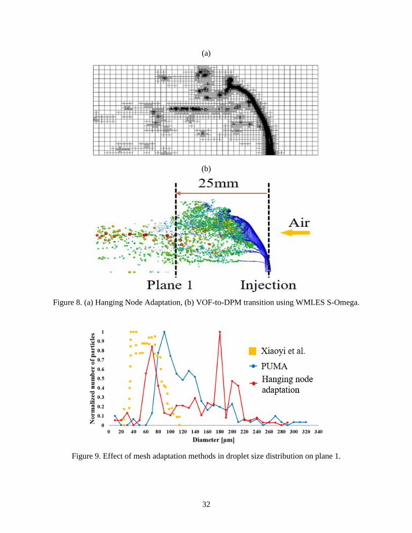
3.2.1 Effect of mesh adaptation methods
One of the methods to simulate a specific droplet size can be by refining areas of interest within
the domain close to a cell size compared to a droplet size; however, it results impractical in some
cases because an excessive mesh is obtained in the domain. Another method is by using mesh
adaptation techniques which were covered in CHAPTER 1. Liquid VOF was used as the variable
for coarsen and refine thresholds. Figure 7 and Figure 8 show the effect of using PUMA and
Hanging Node Adaptation in the cross-section XY midplane. Even though the same turbulence
model, WMLES S-Omega, was used for both simulations, there are some differences in the
liquid atomization process keeping in mind that the PUMA scheme consumed less memory.

31
Droplet size distributions for both mesh adaptation methods can be seen in Figure 9. Both results
were compared to the results reported by Xiaoyi et al. [18] using a maximum droplet diameter as
200μm for the transition criteria. Results for both adaptation methods show larger droplet size
distribution and this is because the current mesh resolution can be considered still coarse.
(a)
(b)
Figure 7. (a) PUMA mesh adaptation, (b) VOF-to-DPM transition using WMLES S-Omega.
32
(a)
(b)
Figure 8. (a) Hanging Node Adaptation, (b) VOF-to-DPM transition using WMLES S-Omega.
Figure 9. Effect of mesh adaptation methods in droplet size distribution on plane 1.
33
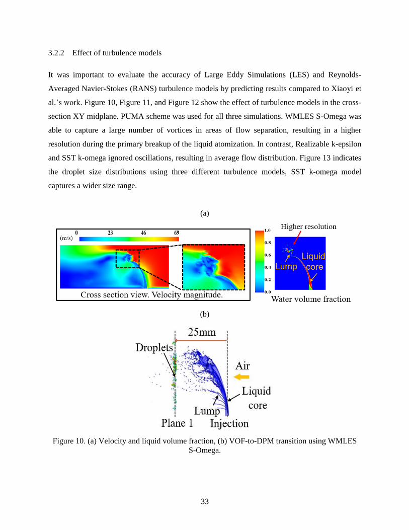
3.2.2 Effect of turbulence models
It was important to evaluate the accuracy of Large Eddy Simulations (LES) and Reynolds-
Averaged Navier-Stokes (RANS) turbulence models by predicting results compared to Xiaoyi et
al.’s work. Figure 10, Figure 11, and Figure 12 show the effect of turbulence models in the cross-
section XY midplane. PUMA scheme was used for all three simulations. WMLES S-Omega was
able to capture a large number of vortices in areas of flow separation, resulting in a higher
resolution during the primary breakup of the liquid atomization. In contrast, Realizable k-epsilon
and SST k-omega ignored oscillations, resulting in average flow distribution. Figure 13 indicates
the droplet size distributions using three different turbulence models, SST k-omega model
captures a wider size range.
(a)
(b)
Figure 10. (a) Velocity and liquid volume fraction, (b) VOF-to-DPM transition using WMLES
S-Omega.

34
(a)
(b)
Figure 11. (a) Velocity and liquid volume fraction, (b) VOF-to-DPM transition using
Realizable k-epsilon.

35
(a)
(b)
Figure 12. (a) Velocity and liquid volume fraction, (b) VOF-to-DPM using SST k-omega.
Figure 13. Effect of turbulence models in droplet size distribution on plane 1.

36
3.2.3 Effect of mesh resolution
A quantitative comparison of the total number of generated droplets based on mesh resolution
can be seen in Table 4. PUMA and WMLES S-Omega turbulence model were used for all three
mesh resolutions. This comparison gives an idea of the requirements for achieving a certain cell
size where the VOF liquid phase after meeting the different transition criteria will be converted
into DPM droplets. The finer the size, the more generated droplets can be analyzed.
Considerations of using the VOF-to-DPM transition model are related to total mesh density,
domain dimensions, other effects explained before, and computational running time since this
model only works using Explicit scheme solver.
Table 4. Mesh resolution and total droplet generated.
Mesh
resolution
Refinement
levels
Cell
size
μm
Droplets
#
41X21X21 5 50 2,700
128X64X64 4 25 13,100
128X64X64 5 12.5 49,900
3.3 Validation
These simulated results are compared to experimental data using Phase Doppler Particle
Analyzer (PDPA) [28] and Xiaoyi et al.’s work [18] . The validation mesh from Figure 6 was
used. Figure 14 illustrates the injection pattern after PUMA scheme takes effect after using 5
levels of refinements. A liquid film and ligaments breakup can be seen. The strong airstream at
69m/s velocity magnitude pushes downstream the liquid injection causing it to atomize, see
Figure 15. WMLES S-Omega turbulence model was used to capture better the complicated
aerodynamic behavior with higher resolution. The mesh will coarsen back up to the original cell
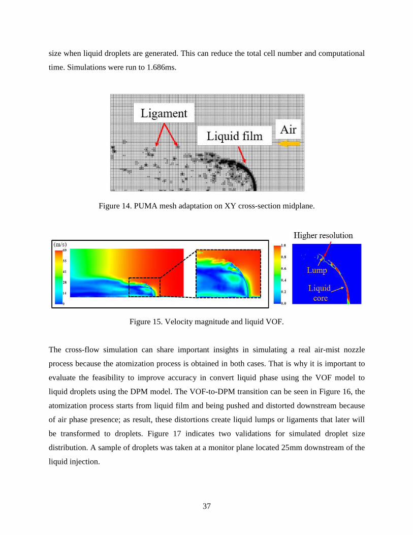
37
size when liquid droplets are generated. This can reduce the total cell number and computational
time. Simulations were run to 1.686ms.
Figure 14. PUMA mesh adaptation on XY cross-section midplane.
Figure 15. Velocity magnitude and liquid VOF.
The cross-flow simulation can share important insights in simulating a real air-mist nozzle
process because the atomization process is obtained in both cases. That is why it is important to
evaluate the feasibility to improve accuracy in convert liquid phase using the VOF model to
liquid droplets using the DPM model. The VOF-to-DPM transition can be seen in Figure 16, the
atomization process starts from liquid film and being pushed and distorted downstream because
of air phase presence; as result, these distortions create liquid lumps or ligaments that later will
be transformed to droplets. Figure 17 indicates two validations for simulated droplet size
distribution. A sample of droplets was taken at a monitor plane located 25mm downstream of the
liquid injection.

38
The first validation shows good prediction compared to the experiment when the maximum
droplet diameter was set to 50μm. The second validation also shows good size distribution
compared to Xiaoyi et al.’s work when the maximum droplet diameter was set to 200μm. The
VOF-to-DPM transition model works better when an accurate input for minimum and maximum
droplet size is specified as well as other considerations previously explained.
Figure 16. VOF-to-DPM transition.

39
Figure 17. Validation for droplets size distribution.

40
AIR-MIST NOZZLE SIMULATION CHAPTER 4.
4.1 Nozzle internal region, Section 1 (VOF model)
4.1.1 Computational domain
A flat fan Delavan Cool-Cast W19917-15 air-mist nozzle was used to develop a methodology
and conduct simulations in this research. The three-dimensional air-mist nozzle can be seen in
Figure 18. Detailed dimensions and internal information are not be included in this research.
Figure 18. Section 1, Delavan Cool-Cast air-mist nozzle 3D geometry.
4.1.2 Boundary conditions and fluid-gas properties
Table 5 summaries all four simulation cases that were run according to the laboratory test report
by Industrial collaborators. A pseudo automatic time step was used. Air as the primary phase
while water as the secondary phase and Implicit VOF disperse interface scheme were used.
Gravity was included in all cases. Water volumetric flow rates were converted from GPM to kg/s
mass flow rates as 0.2837kg/s and 0.4101kg/s, from 4.5 GPM and 6.5 GPM respectively.
Reynolds numbers for the water nozzle were calculated as 26658 and 38535, so k-omega SST
was set for the turbulence model in order to calculate both inner and outer layers for internal
flow.

41
Gas-liquid properties were interpolated based on operating conditions as explained in
APPENDIX A. Constant gas-liquid properties were used during simulations. Surface tension of
0.0724 N/m was set. Water nozzle was set as mass flow inlet, air nozzle was set as pressure inlet,
and nozzle tip outlet was set as pressure outlet at 1 atm.
Table 5. Boundary conditions for simulation cases.
Water inlet
(psig / GPM)
Air inlet
(psig)
60 4.5 30
60 4.5 40
95 6.5 30
95 6.5 40
4.1.3 Effect of mesh types and mesh sensitivity study
The study of mesh types was considered for section 1 of the air-mist nozzle process. Figure 19
compares the meshes using the tetrahedral type and polyhedral type. The tetrahedral mesh done
in ANSYS Workbench shows that if the mesh transition along locations of interest e.g. water
nozzle needs to be smooth, then an excessive cell number is obtained.

42
(a) (b)
Figure 19. Tetrahedral mesh using ANSYS, (b) Polyhedral mesh using STAR-CCM+.
On the other hand, using polyhedral mesh done in STAR-CCM+ obtain a smooth transition with
fewer cells number. A base size between 0.1mm to 1mm, a total number of 10 prism layers with
a thickness of 0.2mm in order to capture flow characteristic close to the wall, and transition
layers ratio of 1.1 was used for both meshes. Other advantages of using polyhedral mesh are
conformal prism layers at corners and a better transition for VOF-to-DPM beyond the outlet
nozzle tip because of the shape of a polyhedral cell. STAR-CCM+ 13.04.010 was only used to
mesh the domain, ANSYS FLUENT 19.1 was used to run all simulations in section 1.
Therefore, polyhedral mesh type with prism layers was chosen to run simulations. A mesh
sensitivity study was conducted using single-phase air with a constant velocity inlet of 1 m/s for
both water and air inlets. Table 6 summaries the increments of cell number, meshing time, and
quality. A surface remesher proximity technique was used to conduct local mesh refinement.
Increment of cell number; thus, mesh time, were obtained by increasing this factor, and it
happens as it was explained in CHAPTER 1. The quality percentage of the cell is improved by
increasing this factor; however, all three cases had a quality percentage greater than 95% with
wall y+ below 2.2.

43
Table 6. Polyhedral mesh sensitivity study.
Surface
remesher
Quality
%
Cells
#
Increment
cells %
Mesh
time [s]
2 95 376,836 0 90
10 97 908,387 141 174
20 98 2,269,811 502 455
Figure 20 illustrates the velocity for all three surface remesher factors along the internal
reference line. Results for all factors do not differ much from each other, major difference can be
seen at the beginning of the mixing section where factor 20 can potentially capture better the
turbulence mixing. However, mesh resolution using factor 2 was used considering computational
time.
(a)
(b)
Figure 20. (a) Internal reference line (b) Velocity along the reference line for all surface
remesher proximity factors.

44
4.1.4 Effect of operating conditions
Four cases were studied where the air pressure and water flow rate were variables. The CFD
analysis was done using the internal reference line as seen in Figure 20. The absolute pressure
can be seen in Figure 21 while Figure 22 shows the velocity magnitude and Figure 23 illustrates
the water concentration VOF for all cases.
Figure 21. Absolute pressure along the reference line.
Increasing air pressure and maintaining fix the water flow rate reduces the water concentration
inside the nozzle. Also, velocities inside the nozzle and at the outlet increase due to a larger
pressure drop and the presence of the air phase. Increasing the water flow rate and maintaining
fix the air pressure increases the water concentration in the nozzle as expected. Also, velocities
inside the nozzle and at the outlet decrease due to the larger presence of the water phase. Some
major differences in the flow were seen at the start of the mixing section.

45
Figure 22. Velocity magnitude along the reference line.
Figure 23. Water concentration VOF along the reference line.
Conditions close to the outlet nozzle tip will be used as the inlet conditions for the external spray
simulations for Section 2, see Table 7.

46
Table 7. Conditions at the nozzle tip.
Cases
(psig and GPM)
CFD Simulation
Water fraction
(Nozzle tip)
Velocity mag. (m/s)
(Nozzle tip)
30 and 4.5 0.38 27.16
40 and 4.5 0.28 35.94
30 and 6.5 0.74 20.35
40 and 6.5 0.57 26.08
4.1.5 Quasi-steady state of simulation cases
A probe point was located close to the nozzle outlet tip in order to check when the solution
reached to quasi-steady state, see Figure 24. A pseudo automatic time step was used, and all
simulation cases start converging at 10,000 iterations, yet 20,000 iterations was chosen as
benchmark for future simulations, see Figure 25.
Figure 24. Monitor point.

47
Figure 25. The convergence of the probe point at 20,000 iterations.
4.2 Spray formation region, Section 2
4.2.1 Computational domain and boundary conditions
Air domain dimensions are determined based on measurement distance during the test by
Industrial collaborators, and the flat fan air-mist spray characterization, see Figure 26. Different
mesh resolutions were used in this section, depending on the goal that will be explained
accordingly. STAR-CCM+ 13.04.010 was used to mesh the domain, ANSYS FLUENT 19.1 was
used to run simulations in section 2 using VOF-to-DPM transition model. Nukiyama-Tanasawa
distribution equation model was run using STAR-CCM+ 13.04.010.
Figure 26. Section 2, spray region.
48
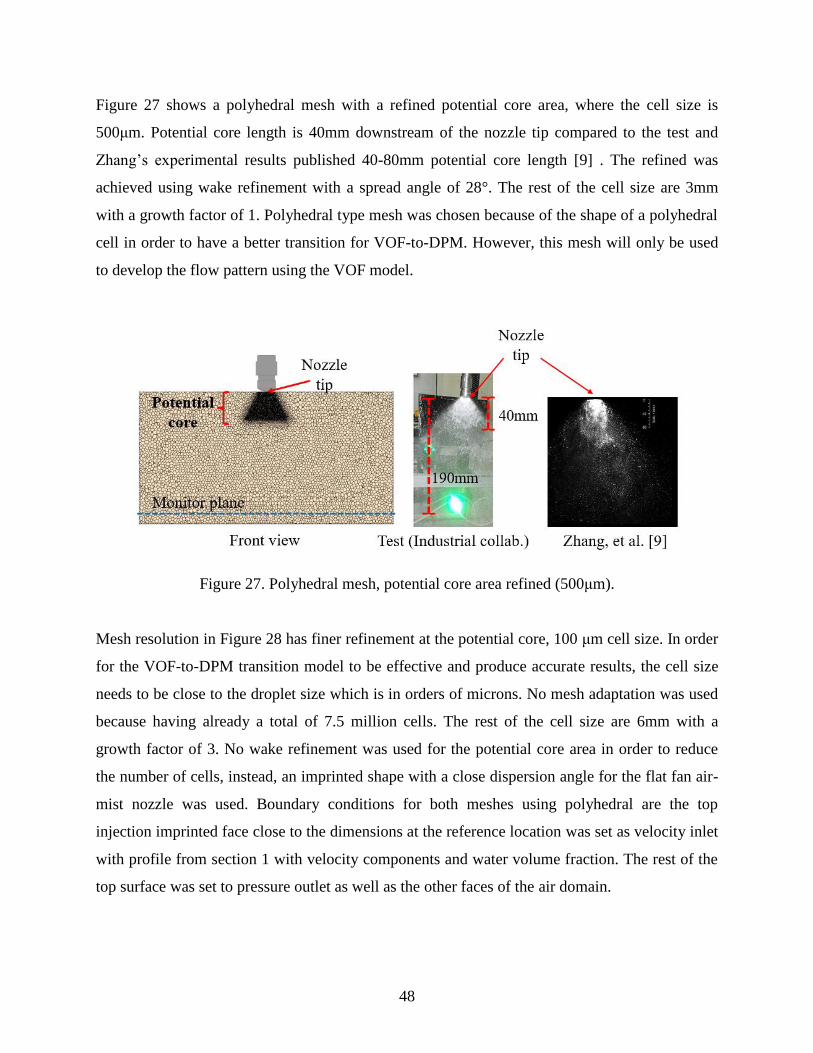
Figure 27 shows a polyhedral mesh with a refined potential core area, where the cell size is
500μm. Potential core length is 40mm downstream of the nozzle tip compared to the test and
Zhang’s experimental results published 40-80mm potential core length [9] . The refined was
achieved using wake refinement with a spread angle of 28°. The rest of the cell size are 3mm
with a growth factor of 1. Polyhedral type mesh was chosen because of the shape of a polyhedral
cell in order to have a better transition for VOF-to-DPM. However, this mesh will only be used
to develop the flow pattern using the VOF model.
Figure 27. Polyhedral mesh, potential core area refined (500μm).
Mesh resolution in Figure 28 has finer refinement at the potential core, 100 μm cell size. In order
for the VOF-to-DPM transition model to be effective and produce accurate results, the cell size
needs to be close to the droplet size which is in orders of microns. No mesh adaptation was used
because having already a total of 7.5 million cells. The rest of the cell size are 6mm with a
growth factor of 3. No wake refinement was used for the potential core area in order to reduce
the number of cells, instead, an imprinted shape with a close dispersion angle for the flat fan air-
mist nozzle was used. Boundary conditions for both meshes using polyhedral are the top
injection imprinted face close to the dimensions at the reference location was set as velocity inlet
with profile from section 1 with velocity components and water volume fraction. The rest of the
top surface was set to pressure outlet as well as the other faces of the air domain.

49
(a)
(b)
Figure 28. (a) Potential core area refined (100μm), (b) Top view injection imprinted face.
A hexahedral mesh type was used to simulate water droplets using Nukiyama-Tanasawa
distribution equation model, see Figure 29. This model assumes no transition from water
ligaments to water droplets, so the domain was considered after the potential core. A total of 0.25
million cells was obtained after cell size varies from 1mm in the top injection imprinted face and
the rest of the domain with cells size of 3mm. Boundary conditions for this mesh are the whole
top surface as velocity inlet mapping the profile after the flow has been developed in section 2
using mesh from Figure 27, all other surfaces as pressure outlet. Gravity and k-omega SST
turbulence model were used for all meshes discussed. Also, fluid-gas properties are referred to as
atmospheric conditions.
(a)
(b)
Figure 29. (a) Hexahedral mesh, (b) top view injection imprinted face (1mm).

50
4.2.2 Spray characterization (VOF model)
Section 1 can be linked with section 2 as explained before in the methodology section by
creating a horizontal cut plane close to the nozzle tip. This plane named top injection imprinted
will contain velocity coordinates and volume fractions for both phases in section 1. Using mesh
from Figure 27, a new isothermal transient simulation with a time step of 1x10⁻³
seconds was run.
Implicit VOF-Compressive sharp interface scheme was used. Velocity boundary conditions were
set by using the plane profiles for all the four cases. As a result, Figure 30 shows the air-mist
nozzle spray characterization for all cases. The condition using 4.5GPM and 30psig shows a
similar velocity magnitude than using 6.5GPM and 40psig. The highest velocity magnitude is
obtained using 4.5GPM and 40psig, while the lowest velocity magnitude is obtained using
6.5GPM and 30psig.
Figure 30. Air-mist nozzles spray characterization.
Figure 31 illustrates the simulated result against the test by Industrial collaborators showing
similarities such as a higher accumulation of water close to the nozzle tip being represented by
10% of the water phase. Also, the air phase presence is strong in simulating an air-mist nozzle.
Droplets should start appearing from the breakup process from the potential core also identified
as the primary breakup region, this will cause the water concentration in the continuous to
decrease. It is recommended that the flow velocity and VOF phases are developed before
droplets start generating. That is why the importance of the current work being discusses.

51
Figure 31. CFD and test spray comparison.
Table 8 summarizes relations of operating conditions and velocity for all cases compared to
measurements. For example, it can be stated that if air pressure is increase, then the velocity of
droplet is increase. On the other hand, if the water flow rate is increase, then the velocity of
droplet is decrease. Even though this comparison should be done against droplets which at this
stage of simulation, there are none, the comparison is done against injected VOF phases and
velocity profiles. These relations also agree with findings published in [10] . Injected profiles
will have a strong influence in droplets trajectory and velocity.
Table 8. Relations of operating conditions and velocity of the air-mist nozzle.
Measurement (Industrial collab.) CFD Simulation
Condition
(GPM & psig)
Avr. droplet
velocity (m/s)
Velocity (m/s)
(Nozzle tip)
Water VOF
(Nozzle tip)
4.5 & 30 17 27.16 0.38
4.5 & 40 22 35.94 0.28
6.5 & 30 14 20.35 0.74
6.5 & 40 17 26.08 0.57

52
A midline at the same monitor reference location as the test across the front view was used to
collect velocity simulated data. Table 9 compares the measurement results for all conditions with
CFD spray characterization simulations, showing similar results among them. Let’s remember
the continuous flow will have a strong influence in droplets; thus, it was important to simulate
the flow characterization before generating droplets.
Table 9. Comparison measurement and CFD continuous at monitor location
Measurement at monitor
location (Industrial collab.)
CFD Simulation at
monitor location
Condition
(GPM and
psig)
Avr. droplet
velocity (m/s)
Max.
velocity
(m/s)
Avr.
velocity
(m/s)
4.5 and 30 17 18.5 17
4.5 and 40 22 23.5 21.5
6.5 and 30 14 15 13
6.5 and 40 17 19 17
4.2.3 Droplet generation methods
Two methods to generate water droplets were proposed in CHAPTER 2.
4.2.3.1 VOF-to-DPM model
The flow developed during the spray characterization will serve as initial conditions to use the
VOF-to-DPM transition model but using mesh from Figure 28. A new isothermal explicit
transient simulation with a time step of 1x10⁻⁵
seconds was set. VOF-Geo-Reconstruct sharp
interface scheme was used. Stochastic collision, wave breakup, and one-way coupling between
DPM and continuous phase were added. A minimum and maximum droplet size of 0 and – 1mm
53
was set. A value of 0.5 for both radius standard deviation and radius-surface orthogonality and a
split parcel factor of 25 were set.
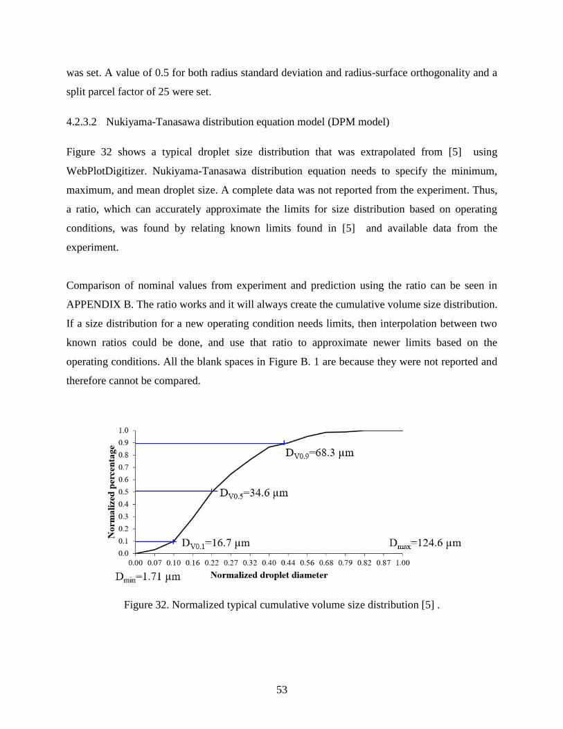
4.2.3.2 Nukiyama-Tanasawa distribution equation model (DPM model)
Figure 32 shows a typical droplet size distribution that was extrapolated from [5] using
WebPlotDigitizer. Nukiyama-Tanasawa distribution equation needs to specify the minimum,
maximum, and mean droplet size. A complete data was not reported from the experiment. Thus,
a ratio, which can accurately approximate the limits for size distribution based on operating
conditions, was found by relating known limits found in [5] and available data from the
experiment.
Comparison of nominal values from experiment and prediction using the ratio can be seen in
APPENDIX B. The ratio works and it will always create the cumulative volume size distribution.
If a size distribution for a new operating condition needs limits, then interpolation between two
known ratios could be done, and use that ratio to approximate newer limits based on the
operating conditions. All the blank spaces in Figure B. 1 are because they were not reported and
therefore cannot be compared.
Figure 32. Normalized typical cumulative volume size distribution [5] .

54
Nukiyama-Tanasawa function distribution needs two specify two more constants, alpha with a
value of 2 and beta with a value of 1. Velocity coordinates from the developed flow as seen in
Figure 30 was set up in the imprinted surface injector. A time step of 1x10⁻³
seconds was used.
Implicit solver and similar models for DPM and continuous were set. The mesh from Figure 29
was used for this simulation.
4.3 Validation
A complete spray simulation can be seen in Figure 33. Only one operating condition was chosen
for validating. Air pressure 30psig and water flow rate 4.5GPM. A side by side comparison is
shown in Figure 34. VOF-to-DPM transition model successfully works generating droplets up to
1000μm. Mesh in some regions in the air domain is still considered coarse, then bigger droplets
will be generated, falling off the expected size range. On the other hand, Nukiyama-Tanasawa
produces a much more uniform droplet distribution. Droplets comparison were done at 0.55
seconds.
Figure 33. Air-mist spray velocity magnitude.

55
Figure 34. Comparison of droplet generation methods.
Table 10 summaries the performance of both droplet generation methods. VOF-to-DPM
transition uses Explicit solver meaning that the time step needs to be accordingly adjusted to
improve conservation. This method requires a high-resolution mesh increasing mesh density and
computational time. Instead, Nukiyama-Tanasawa distribution equation uses Implicit solver, less
mesh, and fast running time.
Table 10. Performance of droplet generation methods.
Approach VOF-to-DPM Nukiyama-Tanazawa (DPM)
Solver Explicit (Δt=1x10⁻⁵
sec) Implicit (Δt=1x10⁻³
sec)
Running time (40 cores) 60 hr 1 hr
Mesh 7.5M 0.25M
Number of droplets Fewer More

56
Simulated droplets measurements were taken on the same monitor plane as the test, about
190mm from the nozzle tip. Results for cumulative droplet size distribution plot for both
methods can be seen in Figure 35. Validation shows that Nukiyama-Tanasawa produces less
percentage difference against test data for droplet size and droplet velocity magnitude. Both
methods can be used to predict droplet aerodynamics behavior.
Figure 35. Cumulative volume size distribution for both methods.
Table 11. Validation for droplet size distribution.
DV0.1(μm) DV0.5(μm) DV0.9(μm) Velocity (m/s)
Test. (Industrial collab.) 75 170 324 17
VOF-to-DPM 10 (86.7%) 200 (17.6%) 480 (48.1%) 20.4 (20%)
Nukiyama-Tanasawa 80 (6.7%) 169 (0.6%) 350 (8.0%) 13.9 (18.2%)

57
AIR-MIST NOZZLES COMPARISON CHAPTER 5.
5.1 Nozzle internal region, Section 1 (VOF model)
5.1.1 Computational domain and boundary conditions
A second flat fan air-mist nozzle is being simulated, see Figure 36. This air-mist nozzle is 35%
smaller compared to the air-mist nozzle in Figure 18, considering the overall length. Details for
internal dimensions will not be discussed. Water pressure of 60psig or its equivalent flow rate of
4.5GPM and air pressure of 30psig were used as the operating condition. Same CFD models and
gas-liquid properties based on the corresponding operating condition as explain before in
CHAPTER 4 were used. The goal of this chapter is to use the developed methodology in other
types of air-mist nozzles and compared them.
Figure 36. Section 1, Spraying System Caster-Jet 3D model.
5.1.2 Mesh sensitivity study
The same mesh type and settings as stated in CHAPTER 4 were used. A mesh sensitivity study
was done using single-phase air with a constant velocity inlet of 1 m/s for both water and air
inlets. Table 12 shows the increments of cell number, meshing time, and quality as the surface
remesher proximity factor increases. The quality percentage of the cell is improved by
increasing this factor with quality greater than 97% with wall y+ below 7.

58
Table 12. Polyhedral mesh sensitivity study.
Surface
remesher
Quality
%
Cells
#
Increment
cells %
Mesh
time [s]
2 97 489,244 0 100
10 97.3 734,828 50 120
20 98 1,517,221 210 201
Figure 37 shows the velocity for all three surface remesher factors along the internal reference
line. The major difference between all three cases can be seen at the beginning of the mixing
section where factor 20 could potentially capture better the turbulence mixing with an increment
in computational time. A mesh resolution using factor 10 was used to conduct the simulation for
this air-mist nozzle in section 1.
(a)
(b)
Figure 37. (a) Internal reference line, (b) Velocity along the reference line for all surface
remesher proximity factors.
59
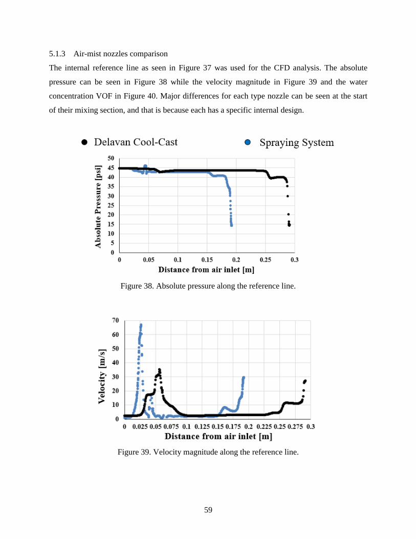
5.1.3 Air-mist nozzles comparison
The internal reference line as seen in Figure 37 was used for the CFD analysis. The absolute
pressure can be seen in Figure 38 while the velocity magnitude in Figure 39 and the water
concentration VOF in Figure 40. Major differences for each type nozzle can be seen at the start
of their mixing section, and that is because each has a specific internal design.
Figure 38. Absolute pressure along the reference line.
Figure 39. Velocity magnitude along the reference line.
60
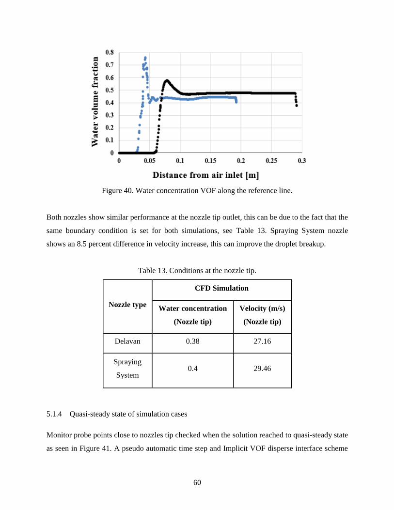
Figure 40. Water concentration VOF along the reference line.
Both nozzles show similar performance at the nozzle tip outlet, this can be due to the fact that the
same boundary condition is set for both simulations, see Table 13. Spraying System nozzle
shows an 8.5 percent difference in velocity increase, this can improve the droplet breakup.
Table 13. Conditions at the nozzle tip.
Nozzle type
CFD Simulation
Water concentration
(Nozzle tip)
Velocity (m/s)
(Nozzle tip)
Delavan 0.38 27.16
Spraying
System 0.4 29.46
5.1.4 Quasi-steady state of simulation cases
Monitor probe points close to nozzles tip checked when the solution reached to quasi-steady state
as seen in Figure 41. A pseudo automatic time step and Implicit VOF disperse interface scheme

61
allow the simulation cases to reach quasi-steady conditions at 20,000 iterations, see Figure 42.
Velocity and water VOF conditions have converged and will serve as inlet conditions for the
external spray simulations for Section 2.
Figure 41. Monitor points.
Figure 42. The convergence of the probe point at 20,000 iterations.
5.2 Spray characterization between nozzles, Section 2 (VOF model)
The continuous flow needs to be developed before conducting DPM analysis. For computational
domain, mesh resolution, simulation settings, and boundary conditions for this simulation refer
to CHAPTER 4. The only difference is to update in the plane profile named top injection
imprinted with the simulation results from section 1 using Spraying System nozzle. If plane
profile dimensions change based on internal design, then a new mesh needs to be done using

62
similar cell sizes as explained before. Figure 43 shows the air-mist nozzles spray
characterization. Streamlines illustrate the internal interaction of fluid-gas. Delavan air-mist
nozzle produces a wider spray and also the primary breakup represented by creating an
isosurface with water VOF of 0.05 is bigger compared to Spraying System air-mist nozzle. The
isosurface water VOF does not change much with values between 0.05 and 0.1.
Figure 43. Air-mist nozzles spray characterization.
Spraying System air-mist nozzle shows a smaller water ligament concentrations in the primary
breakup. I can result in an improved droplets breakup. Figure 44 plots the sprays coverage
showing similar velocities at the monitor plane, yet different effective spray coverage.
Simulations were run up to 0.678 seconds. Simulated results for Spraying System air-mist nozzle
have not been validated yet. However, results show realistic magnitude values close as reported
in [9] . A new simulation using the droplets generation methods covered before can be now
added.

63
Figure 44. Spray coverage at 190mm standoff distance.

64
CONCLUSIONS CHAPTER 6.
6.1 Cross-flow simulation
Computational time changes depending on the turbulence model, mesh adaptation method, and
mesh resolution being used, which is related to the level of accuracy in droplet size needed. A
combination of PUMA and WMLES S-Omega showed good results for validation. PUMA
consumed less memory while running simulations and WMLES S-Omega was more suitable to
better predict the transition from VOF-to-DPM capturing larger and smaller eddies during the
transient gas-liquid interaction.
6.2 Air-mist nozzle simulation
This research focused on the validation of droplets size and droplets velocity magnitude in air-
mist nozzles. Understanding water droplets behavior is very important because they will
eventually impinge the hot steel slab with a certain mass and momentum, the same ones that are
critical for heat removal. A methodology to simulate a complete air-mist spray has been
proposed using Computational Fluid Dynamics (CFD) simulations. The whole atomization
process study can be broken into three independent but linked sections by considering the
computational time. A dispersed VOF interface scheme was chosen to simplify the process as if
there is no sharp separation of phases inside the nozzle. Air-mist nozzle spray characterization
can be simulated using an Implicit VOF-Compressive interface scheme. Where it was found that
if air pressure increases, then the droplet velocity will increase. If water pressure increases, then
the droplet velocity will decrease. Energy consumption should be balanced in practice. Two
methods to generate liquid droplets were analyzed. First, consideration of mesh density is
important if the VOF-to-DPM transition model is planned to be used. The spraying domain could
be simulated by using either a grid adaptive method or by having a constant cell size close to the
droplet size of interest. Second, the Nukiyama-Tanasawa distribution equation model showed
less percentage difference compared to the VOF-to-DPM transition model when validating
models to the test data.

65
REFERENCES
[1] Morelli, U. (2019, September 4). Continuous casting - Modern techniques to solve an old
industrial problem. ROMSOC. Retrieved from https://www.romsoc.eu/continuous-casting-
modern-techniques-to-solve-an-old-industrial-problem/
[2] Spraying Systems Co. Drop Size Comparison Between Hydraulic and Air Mist Nozzles.
Spray technology for steel mills, B-6. Retrieved from https://www.spray.com/-
/media/DAM/Sales-Materials/c/C44B_Spray-Technology-for-Steel-Mills.pdf
[3] Horsky, J., Raudensky, M., & Tseng, A. A. (2005). Heat Transfer Study of Secondary
Cooling in Continuous Casting. AISTech.
[4] TSI. (2019). A sample of phase dropper measurement - Applications providing flexibility
and versatility. Retrieved from https://www.tsi.com/getmedia/3e826f9d-8f05-49e4-9370-
3d32b3fe97da/PDPA%20Applications5001236?ext=.pdf
[5] Schick, R. J. (2008). Spray technology reference guide: Understanding drop size. Spraying
Systems Co., 16.
[6] Horsky, J., Raudensky, M., Moravec, R., & Blazek, K. (2015). Heat transfer coefficients
for the secondary cooling zones in a continuous casting with the effect of steel chemistry.
Ocelary Steelcon.
[7] Frick, J. Important design parameters and user-friendly features of modern air mist nozzles
for slab and beam black casters. Lecher. Retrieved from
https://www.lechler.com/fileadmin/media/fachberichte/metallurgy/lechler_fachbericht_sek
undaerkuehlung_important-design-parameters-and-user-friendly-features-of-modern-air-
mist-nozzles-for-slab-and-beam-blank-casters_jfrick_en.pdf
[8] Ramstorfer, F., Roland, J., Chimani, C., & Morwald, K. (2009). Modelling of air-mist
spray cooling heat transfer for continuous slab casting. International Journal of Cast Metals
Research, 22:1-4, 39-42, DOI: 10.1179/136404609X367290.
[9] Zhang, Y., Wen, Z., Zhao, Z., Huang, J., Wu, W., & Li, B. (2019). Velocity characteristics
of air-mist jet during secondary cooling of continuous casting using PIV and LDV. ISIJ
International, 59(6), 1072-1080, DOI: https://doi.org/10.2355/isijinternational.ISIJINT-
2018-735

66
[10] Cheng, C., Wei, S., Li, Y., Zhou, Y., Qin, X., & Zhu. C. (2019). Study of water droplet
behavior at air-water atomized nozzle with acceleration ring in continuous casting.
STEELSIM, DOI 10.33313/503/063.
[11] Vashahi, F., Dafsari R. A., Rezaei, S., & Lee, J. (2017). CFD simulation of Two-Phase
Flow behavior of a Hybrid Pressure Swirl Atomizer. BEXCO Spring Conference.
[12] Arthur, H., & Vincent G. (2017). Atomization and Sprays. (2nd ed.). Boca Raton, FL: CRC
Press.
[13] Simcenter. (2019). STAR-CCM+ Multiphase Models, 67.
[14] Mugele, R. A., & Evans, H. D. (1951, June). Droplet size distribution in sprays. Industrial
and Engineering Chemistry.
[15] Xianguo, L., & Richard S. (1987). Droplet size distribution: A derivation of a Nukiyama-
Tanasawa type distribution function. Journal of Combust. Sci. and Tech, 56, 65-76,
https://doi.org/10.1080/00102208708947081
[16] Gonzales-Tello, P., Camacho F., Vacaria J., & Gonzalez P. (2008, September 10). A
modified Nukiyama–Tanasawa distribution function and a Rosin–Rammler model for the
particle-size-distribution analysis. Journal of Powder Technology, 186(3), 278-281,
https://doi.org/10.1016/j.powtec.2007.12.011
[17] Hebert, D. A., Schmidt, D. P., Knaus, D. A., Phillips, S., & Magari. P. J. (2008). Parallel
VOF spray droplet identification in an unstructured grid. ILASS Americas, 21st Annual
Conference on Liquid Atomization and Spray Systems.
[18] Xiaoyi, L., Arienti, M., Marcos S., Soteriou, M. C., & Sussman, M. M. (2010). Towards an
efficient, high-fidelity methodology for liquid jet atomization computations. American
Institute of Aeronautics and Astronautics.
[19] Sami, M., Schuetze, J., Hutchinson, P., & Ozarkar, S. (2019). Efficiently modeling primary
liquid atomization using an Eulerian-Lagrangian hybrid model in ANSYS Fluent. ANSYS.
Retrieved from
https://mfix.netl.doe.gov/workshop-files/2019/Presentations/NETL_Aug_7/Session_6/05-
Efficiently_Modeling_Primary_Liquid_Atomization_Using_an_E-
L_Hybrid/Efficiently_Modeling_Primary_Liquid_Atomization_Using_an_E-L_Hybrid.pdf
[20] Sami, M. (2018, May 31). VOF-Lagrangian hybrid spray modeling. ANSYS webinar.
Retrieved from http://storage.ansys.com/webinar/180531-c6f9.mp4

67
[21] Fluent Inc. (2001, November 28). Chapter 23. Grid adaptation. Retrieved from
https://www.afs.enea.it/fluent/Public/Fluent-Doc/PDF/chp23.pdf
[22] ANSYS FLUENT 19.1 theory guide.
[23] Symscape. (2013). Polyhedral, Tetrahedral, and Hexahedral mesh comparison. Retrieved
from https://www.symscape.com/polyhedral-tetrahedral-hexahedral-mesh-comparison
[24] STAR-CCM+ 13.04.010 theory guide.
[25] ANSYS. (2010, December). Lecture 6 Turbulence modeling. Release 13.0. Retrieved from
https://imechanica.org/files/fluent_13.0_lecture06-turbulence.pdf
[26] Reitz, R. (1987). Modeling atomization processes in high-pressure vaporizing sprays.
Atomization and Spray Technology, 3(4), 309-337.
[27] Liu, A. B., Mather, D., & Reitz, R. D. (1993). Modeling the effects of drop drag and break
up on fuel sprays (No. TP-930072). Wisconsin Univ-Madison engine research center.
[28] Leong, M. Y., & Hautman, D. J. (2002). ILASS Americas, 15th Annual Conference on
Liquid Atomization and Spray Systems.
[29] Engineering ToolBox. (2004). Air - Density at varying pressure and constant temperatures.
Retrieved from https://www.engineeringtoolbox.com/air-temperature-pressure-density-
d_771.html
[30] Wikimedia Commons. Air dry dynamics on pressure temperature. Retrieved from
https://commons.wikimedia.org/wiki/File:Air_dry_dynamic_visocity_on_pressure_tempera
ture.svg
[31] Spivey, R.J. (2011). A biotic cosmos demystified. ResearchGate.
[32] Water structure and science. Explanation of the physical anomalies of water F1-F9.
Retrieved from http://www1.lsbu.ac.uk/php-
cgiwrap/water/pfp.php3?page=http://www1.lsbu.ac.uk/water/physical_anomalies.html
[33] Engineering ToolBox. (2004). Surface tension of water in contact with air. Retrieved from
https://www.engineeringtoolbox.com/water-surface-tension-d_597.html

68
APPENDIX A. MATLAB CODE FOR INTERPOLATION FLUID-GAS
PROPERTIES
Fluid-Gas properties
Density and viscosity properties inputs for running CFD simulations are important to generate
realistic flow outcomes. Sometimes simulations results will depend on temperature, pressure
among other variables, so it is significant to add an accurate user-defined function that can
numerically solve right the properties. This section will give an insight into using different
interpolation methods and comparing them to see which one gives a lower percentage difference.
Because air is compressed during an air-mist spray process, then it is a must to calculate the
corresponding gas properties based on operating pressure conditions, refer to Table 5 for
operating conditions in psig units. The laboratory tests by Industrial collaborators, which
simulations are based on, were conducted at room temperature. The air properties are pressure
dependant as seen in Figure A. 1 and Figure A. 2. Both figures data were extracted using
WebPlotDigizer from [29] -- [30] .
Figure A. 1. Air density vs gauge pressure.

69
Figure A. 2. Air viscosity vs absolute pressure.
Figure A. 3 shows the comparison of different interpolation methods to calculate air density
based on pressure. Excel provides different trendlines and the polynomial 2nd
and 6th
orders were
compared. The percentages different are relatively large. Therefore, MATLAB code was used
and exponential least squares and linear least squares methods show lower percentages. The
same comparison can be done with other properties and choosing the simpler but the most
accurate expression can be accomplished. This analysis is important if a user-defined function is
needed to be implemented during the simulation or as in this research to interpolate a constant
but accurate value based on pressure operating conditions.

Fig
ure
A.
3.
Inte
rpola
tio
ns
met
hods
for
air
den
sity
bas
ed o
n p
ress
ure
.
70

71
---------------------------------------------------------------------------------------------------------------------
%%MATLAB CODE
%% air density
clear all
clc
x=[101325.00
135411.74
178180.12
218814.45
278698.91
336442.05
407018.60
492559.01
565280.53
646545.55
714973.51
800521.18
879655.78
971616.53
1061435.96
1153389.44
1253911.86
1330897.86
1405749.80
1519091.11
1681624.79
];
y=[1.26
1.60
2.14
2.61
3.29
3.97
4.79
5.84
6.62
7.61
8.49
9.47
10.36
11.44
12.53
13.68
14.80

72
15.76
16.64
18.03
20.00
];
%%explsqr y=a*exp(b*x) air density
explsqr(x,y)
%%linlsqr y=ax+b air density
linlsqr(x,y)
---------------------------------------------------------------------------------------------------------------------
function explsqr(x,y)
% Construct the least square exponential y=a*exp(b*x)
% that fits x and y row or column vectors.
n=length(x);
n=length(y);
z=log(y);
sumx=sum(x);
sumz=sum(z);
sumx2=sum(x.*x);
sumxz=sum(x.*z);
beta=(n*sumxz-sumx*sumz)/(n*sumx2-sumx^2);
b=beta;
alfa=(sumx2*sumz-sumxz*sumx)/(n*sumx2-sumx^2);
a=exp(alfa);
disp(' Exponential least squares')
fprintf('\n a =%12.16f\n',a)
fprintf(' b =%12.16f\n',b)
disp('_________________________________________________________')
disp(' xi yi ln(yi) a*exp(b*xi) |yi-[a*exp(b*xi)]| ')
disp('_________________________________________________________')
for i=1:n
ye=a*exp(b*x(i));
err(i)=abs(ye-y(i));
fprintf('%6.2f %6.2f %6.2f %12.6f %12.6f\n',x(i),y(i),z(i),ye,err(i))
end
---------------------------------------------------------------------------------------------------------------------
function linlsqr(x,y)
% Construct a least square line y=ax+b
% that fits x and y row or column vectors.
n=length(x);
n=length(y);
sumx=sum(x);

73
sumy=sum(y);
sumx2=sum(x.*x);
sumxy=sum(x.*y);
a=(n*sumxy-sumx*sumy)/(n*sumx2-sumx^2);
b=(sumx2*sumy-sumxy*sumx)/(n*sumx2-sumx^2);
disp(' linear least squares')
fprintf('\n a =%12.16f\n',a)
fprintf(' b =%12.16f\n',b)
disp('_________________________________________________________')
disp(' x y a*x+b |y-(ax+b)| ')
disp('_________________________________________________________')
for i=1:n
yl=a*x(i)+b;
err(i)=abs(yl-y(i));
fprintf('%6.2f %6.2f %12.6f %12.6f\n',x(i),y(i),yl,err(i))
end
err=sum(err.*err);
fprintf('\n E(a,b) =%12.6f\n',sum(err))
---------------------------------------------------------------------------------------------------------------------
The water properties show less pressure dependant as seen in Figure A. 4 and Figure A. 5. Both
figures data were extracted using WebPlotDigizer from [31] -- [32] .
Figure A. 4. Water density vs pressure.

74
Figure A. 5. Water dynamic viscosity vs pressure.
Because air-mist nozzle has the presence of air and water phases, the surface tension of
0.0724N/m was used as [33] to have a realistic simulation.

75
APPENDIX B. RATIO APPROXIMATION TO FIND LIMITS IN
CUMULATIVE VOLUME SIZE DISTRIBUTION
Based on operating conditions
Figure B. 1. Size distribution for 30psig – 4.5GPM.
Figure B. 2. Size distribution for 40psig – 4.5GPM.

76
Figure B. 3. Size distribution for 30psig – 6.5GPM.
Figure B. 4. Size distribution for 40psig – 6.5GPM.

77
PUBLICATIONS
Mosquera E, et al. Numerical Model Development for Air-mist Spray in Steel Secondary
Cooling Process Using the VOF-to-DPM Multiphase Transition Model [C] AIST 2020
(published)
Moreland J, Estrada J, Mosquera E, et al. Integrating Fluid Simulation with Virtual Die Casting
Machine for Industry 4.0 and Operator Training [C] TMS 2020 (published)