aid-fl133 023 life cycle dynamic environment(u) force …
TRANSCRIPT

AID-fl133 023 LIFE CYCLE COSTING IN A DYNAMIC ENVIRONMENT(U) AIR i/3FORCE INS OF TECH WRIGHT-PATTERSON ARE OH J A LONG1983 AFIT/I NR
UNCLASSIFIED FG51 N
mohhhmhomioiII fflfflffl|lflflfflfmEE||hhh|h|hhhImhEE|h|hEEEEEEEhh|hhhhhEEEEE~I fffflllflf|lfllffl

1.0-
L2MaM
1111151 1. W6
MICROCOPY RESOLUTION TEST CHARTNATIONAL BUREAU OF STANDARDS -1963-A

'" UNtO ASSSE ILRITv -LASSIFICATI N 3F TIS PAGE ,,When ") t
REPORT DOCUMENTATION PAGE WE A D rNL, i. -,.
SI REPORT NUMBER 12 GOVT ACCESSION NO ECIP IENr" "-AT&7- , wmjiFI
AFIT/CI/NR 83-26D -133 0;2. 4 TITL F ind Subtltlt ) If Tr -- _F __P__T F;4 0C -J.-Q O
ct Life Cycle Costing in a Dynamic Environment 1WNU/DISSERTATION
A0HRs 6 RCMNTP R 3 l 'BR
John Amos Long
9 PERFORMING ORGAN.ZA'ICN NAME AND ADDRESS 10 PROGRAM ELEMENT PRCJE."r
TA
AREA a *CRK j4IT '4u v E 'S
AFIT STUDENT AT: The Ohio State University
'I I CCNTROLLING OFFICE NAME AND ADDRESS 12 REPORT DATE
AFIT/NR 1983
WPAFB OH 45433 13. NUMBER OF PAZES189
14 MONITORING AGENCY NAME & ADDRESSrit differ.nt from Co.nrolling Oilice) 15. SEC'JRITY CLASS (O " 0',e 'rppr
UNCLASSIS., DECLASSIFICATiON DOWNGR-rA NG
SCHEDULE
16. DISTRIBUTION STATEMENT (of this Report)
APPROVED FOR PUBLIC RELEASE; DISTRIBUTION UNLIMITED
'7 DISTRIBSJTION STATEMENT tot the abstract entered in Block 20, If different from Report)
16. SUPPLEMENTARY NOTES
APPROVED FOR PUBLIC RELEASE: IAW AFR 190-17 "e Ic: ;-)...-
S ,E P .Air Fge te l T C t
1S KEY WORDS (Continue on rei'ere side it nece wsry and identify by block number)
20 ABSTRACT (Continue nn reverse side If necessary and Identify by block number),. "
ATTACHED
DD 1 , 1473, S',-.-- IS n,,3LETE UNCLASS
41.-.

IAe-i-sqon For
LIFE CYCLE COSTING
IN A
DYNAM IC ENVIRONMENT
DISSERTATION APresented in Partial Fulfillment of the Requirements foE
the Degree Doctor of Philosophy in the Graduate
School of The Ohio State University
By
John Amos Long, A.8. M.A*, M.S.
The Ohio State University
1983
Beading Committee: Approved By
Gordon M. Clark
Valter C. Giffin
Clarence H. Martin .jt"1 /
Department 'of Industrialand Systems Engineering

LIFE CYCLE COSTING
IN, A
DYNAMIC ENVIRONMENT
By
John Amos Long, Ph.D.
The Ohio State University, 1983
Professor Walter Giffin, Adviser
The consideration of life cycle cost is a major part of the
Department of Defense management strategy to control the increas-
ing cost of defense systems. It includes the cost of research
and development, production, operating and support, and disposal.
Unfortunately, due to a lack of credibility, life cycle costing
has not reached its full potential. In ah attempt to rectify the
situation, this research centers on life cycle costing in a
dynamic environment. This examination is from three perspectives:
methodology, modeling, and application. The chapter on methodology
is a critical examination of Air Force life cycle costing in the
acquisition of new aeronautical systems. It contains recouixenda-
tions for reorganization and revision of current business prac-
tices. The chapter on modeling reviews various models and methods
for risk analysis including Monte Carlo simulations, additive and
I C Ks

" "- -- .
-. 2
multiplicative moments, sums and products of random variables, and
transform techniques., These methods are then directly applied to
the problem of operating and support cost estimation. Included is
a discussion of candidate probability distributions and suggestions
for presentation of the risk analysis. -Ahe chapter on application
demonstrates the feasibility of using the various models and methods
under a realistic scenario for systems acquisition. Therefore, in
order to enhance the credibility of life cycle costing, all three
aspects (methodology, modeling, and application) are necessary. With
its intuitive appeal and following the recommendations\and procedures
set forth in this research, life cycle cost holds great potential in
managing the nation's defense resources.
Key Words: Life Cycle Cost, Risk Analysis
Rank and Service: Major, U.S. Air Force
Pages: 199
. . . . . .9'

ACKNOVLEDGEMNNS
I wish to thank ay adviserl Dr. Halter Giffin, and the re~-
mainder of my research committee for their guidance, pa-
tience, and understanding in completing this task. I1 also
wisk to thank Dr. Darrell Roach for his assistance in pr~e-
paring for the interviews conducted as a part of this re-
search.
My appreciation is also extended to all those w~ho submit-
ted themselves to the interviews and, in particular, to MrL.
Vera Menker for his help in arranging and scheduling th in-
terviews.
I extend my gratitude to my wife, Nancy, and dauyjhters,
Any and Abigail$ fo -r their love and support through this or-
deal. Above all, I thank and praise the Lord for His pres-
ence and grace in times of trial.

VITA
October 27, 1946 ....... Born - Harrisburg, Pennsylvdnia
A.B., Miami University. Orford,Ohio
Entered Active Duty - UnitedStates Air Force
1968-1977 .............. Navigator and Radar Navigator,* B-52, Vurtsmith AFB, Michigan,
Seymour-Johnson AFB, NorthCarolina
1976* .................. a.&., Central MichiganUniversity, Mt. Pleasant,Michigan
* 1978.................... M.S., Air Force Institute ofTechnology, Wright-PattersonAFB, Ohio
1979-1980 ............ Life Cycle Cost Analyst, AirForce Acquisition Logistics
• .Division, Vright-PattersonAFB, Ohio
1980-1983 .............. Student, Department of* Industrial and Systems
Engineering, The Ohio StateUniversity.,?
FIELDS OF STUDY
Rajor Field: Industrial and Systems Engineering
Studies in Operations Research. Professors Walter C.Giffin, Gordon 8. Clark, and Clarence H. Martin
Studies in Logistics Engineering. Professors Walter C.Giffin and Gordon f. Clark
- iii -
4 . . .. . .

.Studies in applied Statistics and Experimental Design.Professor John B. Neuhardt
-iv
.5
.5
.5 % .; ? .. .. . .. - .. ; . . .. . . -'.. -. . ... ,. ,

-a
TABLE OF CONTENTS
. ACKIOELEDGERENTS ................... ii
VITA .... a.... aa.. a a..... . . iii
LIST OF TABLES . . . . .. ........ vii
LIST OF FIGURES . . . . . . . . . . . . . . . .. . ix.,
ChapterPle
. INTRODUCTION .. . . . . . . . . . . . . . . . . . 1
LCC Defined .. . . . .a a 3Uses of LCC Information a a a. . a . . 5LCC Management . aa a..a . 6Estimating Techniques .. a...7
Risk and Uncertainty ... .aaa 11Sources of Uncertainty . . .. .. . 12Capturing Risk and Uncertainty . 13
Research Question . .a a a a..... .. 14
I. ETHODOLOG! . a. . a . . . . . . . . . . . .. 15
The Air Force Acquisition Process . . . . a . 1bThe Air Force LCC Structure . . .. .a. 18
The Directives . .a . . . .. . 13The Organizations - . . .a .-. . .. . a 20
The Credibility Gap .. . . . . .. . o . . 25The Estimate in Perspective . a .. . . . 27Program Uncertainty . a . o . . 30The Program Manager . . . . . . 33The People Problem .. . . .a a . . . 34The Data Problem .. . . . .a a 35The Modeling Problem .a . . . . .a a 3,3
The Role of Risk Analysis . .. . . . . 41Conclusion .. . . . . . . . . . . .a a .a . 45
I1. MODELING a aa a a .. a a 47
Models and Modeling Methods a49
Monte Carlo Simulation .a a . 50Analytical Methods . . . a a a a a a a .. 54
Additive and Multiplicative Moments 54Sums and Products of Random Variables 60
-iv-
-- * -*. -

777,
Transforms ........ . 65Modeling OSS Costs ...... .. . . . 74
The Basic Building Block . . . . . . . . . . 74Total OSS Cost . . . . . .. . . . . . . . 76
Inflation . .. .. .. .. ...... 78Discounting ......... .80
Individual Cost Elements . . . . . . . . . . 83Probability Distributions . . . .. . . . . 92
The Normal Distribution . . . . . . . . . . 94Central Limit Theorem . . . . . . . . . . 96
The Log Normal Distribution . . . . . 98The Triangular Distribution . . . . . . . . . 99The Beta Distribution . . . ... 100
The Rectangular Distribution . . 103The Gamma Distribution . . . a . . . . 104The Poisson Distribution . . . . .. . . 106
Presenting the Risk Analysis . . . . . . . . 108
IT. APPLICATIONS . . . . . . . . . . . . . . . . 114
The General Approach . . . . . . . . . . . 114Subjective Inputs . . . . . ......... 116The Scenario......... . .. . .. . 119Most Likely Point Estimate . . . . . . 121Preliminary Risk Analysis . . . . . 123
Yearly Cost Computation . . . . . . . 123Maintenance Personnel . . . . . .. 123Fuel . . . . . . . .. . .. . . . . . 126Depo.t Maintenance . . . . . . . . 12')Replenishment Spares . . . . . . 130Engine Spares - . ...... . . 131Avionics Spares . . .... . . . 134
Total Discounted Cost Computation . . 136Presenting the Analysis . a . 140
Indepth Risk Analysis . a . . . . a . a . 143Fuel . . . . a. a . a. . . .. . 143Engine Spares .. . . .a a 145Depot Maintenance . a . . . . . . 146
Sensitivity Analysis . . a . . . a . . .. 14dConcluding Remarks . . . . a a. . a . . 143
V. SUNNARY. RECONBEUDATIOISg IND FUTURE STUDIES . . 151
Methodology . . . a a . . . a a a a a . a . 152Model rIng . . a a a0 a a a . a a a a a a 0 194Application . . a 156Fecomaendations o 156Future Studies .... a .aaaa .aaaa . 157
.5
.5 " , .' ." . . -. .." " I " -" -, "' " " , ' '" " " ' ' " " " ' " " ' " " " " " " " " '

Ao X............ER ................ 19
AD-pendix p-
A. INTBRVIEV ROSTER . . . . . . . . . . . . . . . 159
B. GENERAL INTERVIEI QUESTIONS . . . . . . . . . . . 161
C. ORGAINIZATIONAL SPECIFIC INTERVIEV QUESTIONS . . . 163
D. THE TRIANGULAR DISTRIBUTION . . . . . . . . . . . 166
Le MAINTENANCE PERSONNEL CALCULATIONS .... . . . 168
F. FUEL CALCULATIONS . . . . . . . . . .. . . . . . 169
G. ENGINE SPARES CALCULATIONS . . . . . . . . . .. 170
He AVIONICS SPARES CALCULATIONS . . . . . . . . . . 172
X. COST ELEMENT VARIANCE SUMMART . . . . . . .. . . 174
J. BILLIN TRANSFORM EI&UPLE - FUEL CER . . . . . . . 176
K. HELLIN TRANSFORM EXAMPLE - SPARE ENGINE CER - . . 178
L. LAPLACE TRANSFORM EXAMPLE - DEPOT MAINTENANCE . . 180
BIBLIOGRAPHY . . . . . .. . . . . . . . . . . . . .. 181
vi

48
LIST OF TABLES
, Table P-"2
* 1. OSS Cost Element Structure . . . . . . . . . . . . . 10
2. Interview Summary ....... ................. 4b
3. Additive Moments . . . . . . . . . . ......... 57
4. Additive to Multiplicative Moments ..... . . .5
5. Multiplicatve to Additive Moments ............. 51
6. Additive Model Formulae ............
7. Multiplcative Model Formulae . . ........... 63
8. General Additive Model Formulae . ...... ... 64
9. Conversion- Origin to Central Moments . . . ... 72
10. Probability Distribution Summary ......... . 107
4 11. Two-Sided Tolerance Factors . .......... .. 111
12. FoF Preliminary Cost Analysis . ......... . 121
13. Maintenance Personnel Requirements .. ......... 123
* 14. Maintenance Personnel Calculation Summary .... 124
15. Maintenance Personnel Pay . . . . . . . . . . . . 125
* 16. Maintenance Personnel Yearly Pay Summary ..... 126
17. Fuel CER Variable Values .. . . . . . . . . . 129
18. Yearly Fuel Cost Summary . . . . . . . . . .. . 129
19. Depot Maintenance Cost . . . . . . . . . . . . . . 130
- vii -

20. Depot Maintenance Yearly Cost Summary ........ 131
I21. Spare Engine CER Variable Values . . . . . . . . . 133
22. Engine Spares Yearly Cost Summary .. .. .. .... 133
23. Spare Avionics CER Variable Values . . . - . . . 135
*24. Avionics Spares Yearly Cost Summary ......... 135
25. Risk Analysis Yearly Cost Summary......... 136
26. Fuel/Spares Correlation . . . -.. .. .. .. .... 137
27. Phase In/Phase Out Yearly Cost Summary. ....... 1393
28. Discounted Total O&S Costs . . -.. .. .. .. .... 140
.4
77 7I
LIST OF FIGURES
1. Veapon System Costs ...... ...... . 5
2. Aircraft Sys Acq LCC Organizational Chart . 24
3. Effect of Program Decisions on Total LCC....... 26
4. Estimating Technique Applications . .. . .. . 40
5. LCC Decision Making . . . ... . . . .............. .
6. Impact of Cost Risk on Decision Making . . .. . 43
7. Cost Variable Breakdown . . . . . . . .. .
8. Monte Carlo Simulation Approach .. . . . .. . 52
9. Simulation Example Distributions . . .. . . . . 52
10. Typical System OSS Cost Profile .. . . . . . . 7C
11. Time Series Example . . . . . . . . ................. 8u
12. Time Series Collapsed . . . . . . . . . . . .85
13. Modeling Structure . . . . . . . . ...-..... . 91
14. Mean-Variance Plot . . . . . . . . . . . . . . . . 109
15. Cumulative Distrbution Function Plot . . . . . . . 112
16. Floating Bar Graph . . . . . . . . 113
17. FoF Mean-Variance Plot . . . . . . . .. . . . . 141
- IX -
4.,

Chapter I
I NTRODUCTIONI
In these times of economic difficulty and deficit budigets,
the high cost of defense systems and rapidly increasing cost
of supporting them once they are deployed is of great con-
cern to the Department of Defense (DOD). The need for af-
fordable equipment in terms of both initial cost and support
cost becomes more critical as the present budget trends con-
tinue. To combat this problem, the application of the life
cycle cost (LCC) concept is receiving greater emphasis. The
LCC concept was introduced in the DOD in the early 1960's
primarily because of increasing concern over the consequenc-
es of competitive procurement without regard to total life-
time cost of a weapons system'. Today, LCC is a major part
of the DOD management strategy to control the increasing
cost of defense systems.
'A system is a separate, identifiable entity for whichcosts can be accrued and tracked. What may be a systemfrom one perspective may be a subsystem or component partfrom another. Thus, a system, for example, may be an air-craft, its electrical system, or an avionics componentsuch as an inertial navigation unit.
.. . .* .. ..
.2. . . . . . ..-

-% -Z r._7;
2
Prior to the inception of LCC, the federal government
3 customarily sought to buy the least expensive product avail-
able [95:1]_ Contracts normally were awarded to the lowest
bidder. Although there were exceptions, this practice re-
suited in the acquisition of many weapons systems that were
expensive and difficult to maintain. The essential missing
element not considered was the cost of ownership, the cost
of operating and supporting weapons systems. Quoting from
Defense Procurement Circular 115, dated 24 September 1973,
Since the cost of operating and supporting thesystem or equipment for its useful life is sub-stantial and, in many cases, greater than7 the ac-quisition cost, it is essential that such costs beconsidered in development and acquisition deci-sions in order that proper consideration can hegiven to those systems or equipments that will re-suit in the lowest life cycle cost to the govern-ment.
*Thus, the objective of life cycle costing is to enable deci-
sion makers, during early program phases, to consider all
costs of ownership, as well as, those development and acqui-
sition costs which are closest on the fiscal horizon.
Unfortunately, life cycle costing has not reacheJ its
full potential. One reason is a lack of credibility in the
LCC estimate on the part of managers, decision makers, ani,
even, cost analysts. Life cycle costing concerns future
costs. Consequently, life cycle costing methods and techni-
ques must deal witb risk and uncertainty. Because of this
risk and uncertainty, they, the users, do not know how much

3
confidence to place in the LCC estimate. In an attempt to
rectify this situation, this research will examine life cy-
cle costing in a dymanic environment. This examination is
from three perspectives: methodology, modeling, and arplica-
tion.
1.1 LCC DEFINED
LCC, as defined in Air Force Manual (AFM) 800-11, is "the
total cost of an item or system over its full life. It in-
cludes the cost of acquisition, ownership (operation, main-
tenance, support, etc.) and, where applicable, disposal."
Acquisition cost includes the cost of research, development,
test and evaluation (RDT&E),z production3 or procuremznt of
the end item; and the initial investments required to estab-
lish a product support capability (e.g. support equipment,
initial spares, technical data, facilities, training, etc.).
Ownership cost includes the cost of operation, maintenance,
and follow-on logistics support of the end item and it3 as-
sociated support system. The terms "ownership cost" and
2 Research and development costs are those costs associatedwith the research, development, test, and evaluation ofsystem hardware and software. it includes the cost forfeasibility studies; simulation and modeling; engineeringdesign, development, fabrication, assembly, and test ofprototype hardware; initial system evaluation; associateldocumentation; and test of software.
3 Production costs are those costs associated with producin;the aircraft, initial support equipment, training, techni-cal and management data, initial spares and repair parts,plus many other items required to introduce a new system.
; ? - i . i i .i .. . ..... . . .. .

4
"operating and support (OS) cost" are synonymous. Thus, p
the four major cost categories included in the LCC estimate
are research and development, production, operating and sup-
port, and disposal.
Figure 1 illustrates the need for LCC. Acquisition cost
is but the tip of the iceberg. Depending on the system and
the length of the life cycle, ownership costs can far exceed
the acquisition cost [73:1-1]. "The LCC technique is justi-
fied whenever a decision must be made on the acquisition of
an asset which will require substantial operating and mair.-
tenance costs over its life span" [15:1]. But, life cycle
costing is not limited to acquisition decisions alone.
I I
I I
. II I
I I
Figure 1: Weapon- Syste Cost

1.2 sJ __ L" I!!oINnATIO3
The LCC estimate has many and varied uses. Seldon
(95:11-12] lists six primary uses of LCC:
1. Long range planning
2. Comparison of competing programs
3. Comparison of logistics concepts
4. Decisions about the replacement of aging equipmen~t
5. Control over an ongoing program
6. Selection among competing contractors
In addition, May [69:2-3] lists the following uses of LCC
estimates:
1. Support of budget estimates
2. Design-to-Cost (DTC)' programs
3. Management reviews
These uses all equate to one common purpose: LCC aids de-
cision makers by supplying information to assist in the de-
cision process. Thus, life cycle costing is really a con-
tinuous management process the object of which is to ensure
that new acquisitions meet operational needs at the lowest
life cycle cost [6:1].
A management concept wherein rigorous cost goals are es-tablished during development and the control of systemcosts (acquisition and operating and support) to thosegoals is achieved by practical tradeoffs between opera-tional capability, performance, cost, and schedule.
.4o
6
1.3 LCC I.&!AEBEN
As a management tool, LCC is supposed to be considererd by
all Air Force personnel in making decisions related to the
selection, design, development, procurement, production,
modification, repair, and use of defense resources. To car-
ry out this mandate, factors which significantly impact LCC
must be identified and meaningfull tradeoffs explored. Such
tradeoffs involve the selection of design and cost goals,
acquisition strategy, sources of goods and services, and
support concept. For a new acquisition, the program manager
is responsible for LCC management efforts, as well as all
other aspects of program management. Life cycle cost man-
agement efforts must be tailored to each individual progcaa
and include proper documentation of LCC activities, studies,
* and analyses to support program decisions. The focus of
such studies and analyses is the estimate itself. Depending
. upon the program phase and information available, several
-' techniques are available for arriving at an estimate of to-
tal LCC.
1.4 BSTINUA _g TSCnZQolS
The three most often used cost estimating techniques in the
Air Force are analogy, parametric estimation, and engineer-
ing estimation. Analogy is, perhaps, the simplest of the
three. The amalyst begins by identifying an existing system

7
that is similar to the system of interest. The cost of the
system of interest is then estimated by taking the cost of
the existing system and adjusting it to account for differ-
ences between the two systems. Although widely used, analo-
gy has several limitations. Analogy places heavy reliance
on the opinion of experts to determine the similarities and
differences between the two systems. Two experts, given the
same information, often have different opinicns. Thus, the
analysis may not be reproducible, may not be traceable, and
may be difficult to document. On the positive side, esti-
mates using analogy are usually fairly easily and quickly
done. Analogy is used mainly in the early stages of weapons
system development when the least is known about the final
end product.
" Parametric costing involves the use of a cost estiniatinj
relationship (CER). A CER is a mathematical equation or
model that relates one or more characteristics of the system
to cost. It is a function of one or more independent vari-
ables which yields cost as a dependent variable [75:46).
The equation can be simple or complex, linear or non-linear.
For example, a CEB may be
Airframe cost = Pounds of metal x Cost per pound
+ Labor hours x Cost per hour
or
Airframe cost = Veight2 x Speed3 .
"-i' -i k ~ ' i .. / . 'ii'-'-, -.' - ,, .-- - . '. ,.i. * - " . .• " -

8
CERs are developed through analysis of past data, often in-
volving regression analysis. CERs are used when system
hardware has been defined and physical characteristics are
available.
The third estimating approach is the "grass roots" or en-
gineering method, also known as the bottom-up approach. The
analyst begins at the lowest level (highest level of detail)
and works up adding costs as they occur. This method re-
quires detailed knowledge of the system. The drawback is
that intricate detail is needed and, by the time the analyst
is able to apply this method, it is usually too late to sig-
nificantly influence crucial design and support decisions.
Cost estimating models using any or all of these methoJs
generally fall into the broad class of models known as ac-
counting models. Accounting models begin with a cost ele-
ment structure (CES) which is simply a list of the cost
items or categories to be included in the final estimate.
All relevent cost categories should be included. The cost
elements are then added or "accounted for" in arriving at
the total cost. The Air Force approved CES for O&S cost is
shown in Table 1
Those cost elements which make a significant contribution
to the total cost are known as cost drivers; they require
special attention from the analyst for it is among these
that decision makers will be looking for tradeoffs to reluce

Cd z
to Cd to4g 4 ~ + Pq+ ~ 42+ 00 i-i
P-4Z r,.P.+ >tCJ Z "Z 0 E-
:: +i47 0 E-4 0 68 E-U) -3 JL 00 CdM ) ri Z 044-'
H "-H rI -H-H 2.-4-i -rq ' 44Pr 4-iE-4 0H > P-4 H > Cd H > 0 0 r1 .4 z cr10 W .H
.' i *-ri-I ri -i U ri ri E4 0 0$4 z z br.4 >
0a C 0 .rw0G r,0 &0
'-4 '-4
+3
C) 0+2 43
o C/
E-4 H ~ HC)t1 a
0 s-4 -4 z 0 E-4 4~ &I-I 4) -4 4-3 CdW C
E-1~~ 0 w C41 ) -P t 4J+2/ - brzi 4 /0 9 E-4 CS-G)r rj p~
p.4 wi P-r Z 4) 4 car)~ 0HZ+-I a)+20-40.C+4 Cr1 0 -00 g w x0t
0 - 4.-3' +1 HW + 9 40 a g ) 0 +-1 4 Enr=) a
am 920 cr1 2 L) 4 q. 4 E4.450 0 + 0 4) zQ)0+'- (;-4 t-4 $4 0 P4 44 'd4 "O/CO0 ~0r
I-4 C/4) ) 4
TABLE1
065 Cost Element Structure

10
cost. This is not to say, however, that other cost elements
should be ignored. A previously ignored element may sudden-
ly turn into a cost driver. For example, fuel costs were
once insignificant when compared to other operating costs.
Now they are quite significant and fuel conservation m~eas-
ures are receiving the highest priority.
There is no specific cutoff point for determining cost
drivers, nor does a sudden change alone necessarily produce
a cost driver. The selection of cost drivers is at the dis-
cretion of the analyst or at the direction of decision mak-
ers.
1.5 RISK IND UNCERTAINTY
All aspects of life in the world are subject to risk and un-
certainty. Risk and uncertainty are key characteristics cnf
any l:ong range planning and cost estimation. Few, if any,
decisions are made under conditions of certainty and without
risk. Due to the complexities involved, analysts and deci-
sion makers must specifically and explicitly address this
risk and uncertainty in performing their assigned tasks.
Although the terms risk and uncertainty are often used in-
terchangeably, they are not the same. Risk is the probabil-
ity that a planned event will not be attained within con-
straints (cost, schedule, performance) by following a
specified course of action [64:18]. Uncertainty is incom-

,-,o,-11
plete knowledge [64:18]. Fisher [34:202] says, "A risky
situation is one in which the outcome is subject to an un-
controllable random event stemming from a known probability
distribution. An uncertain situation, on the other hand, is
characterized by the fact that the probability distribution
of the uncontrollable random event is unknown." Canada
[18:252] relaxes these definitions somewhat by concluding
that risk is the dispersion of the probability distribution
of the element under consideration while uncertainty is a
lack of confidence that the probability distribution is cor-
rect. It is the task of analysts to try to reduce uncer-
tainty to risk and then to meaningfully convey the risk to
decision makers.
1.5.1 Sources of Uncertaint
There are two primary sources of uncertainty affecting LCC
estimates. These are environmental uncertainty and cost es-
timating uncertainty. Environmental uncertainty is the
product of unforseen changes in politics, engineering, quan-
tity, support concept, schedule, policy, requirements, use,
or life cycle. These environmental changes are outside the
control of cost analysts. If these areas are held constant,
there is still some uncertainty, cost estimating uncertain-
ty.
5"' " % ' °% " ° ' °
" ' "" " " "" " " " " - " - '

12
Cost estimating uncertainty is more easily addressed by
analysts. It stems fLom an inability to measure cost pre-
cisely, inadequacy of applicable data, statistical uncer-
tainty, errors or inconsistencies in the treatment of data,
and errors in judgement (57:3-10]. Thus, cost estimatin,
uncertainty has both statistical and subjective aspects.
The subjective aspect is introduced in conducting the analy-
sis itself. The assumptions used and the decisions male by
analysts in performing the study are a source of subjectivc
variance The statistical aspect results from the reduction
and analysis of historical data and the modeling methods anI
techniques employed. Because this research is primarily
concerned with cost estimating uncertainty, a 'fixed scenar-
io' with respect to environmental uncertainty is assumei.
Both the statistical and subjective aspects of cost estimat-
ing uncertainty will be addressed.
1.5.2 C ing Risk and Uncertaintl
Analysts cannot eliminate risk and uncertainty from a pro-
gram. At best, they can present and explain the aspects of
risk and uncertainty impacting the program. This is done
through risk and sensitivity analysis.
Risk analysis is a procedure for analyzing how randomness
affects the total cost. To place a cost estimate in propeu
perspective, it must be viewed as a random variable. By

13
definition, a random variable is a numerically valued func-
tion defined over the sample space [47:327]. Unfortunately,
the application of risk analysis, particularly in the case
of OSS costs, seems limited. &uthors and analysts, such as
Large [61], McNichols [71], and Worm [104], have addressei
the problem of risk in hardware cost estimation, but fei
have examined OSS cost. A notable exception is Dienemann
(27].
Uncertainty is addressed through the application of sen-
sitivity analysis. Although often mistakenly used as a sub-
stitute for risk analysis, sensitivity analysis is designc]
to systematically explore the implications of varying as-
sumptions about the future environment and is normally cen-
tered on the cost drivers where a range of alternative pa-
rameters is investigated. The objective is to identify
those parameters whose change will impact the decision at
hand. Risk analysis and sensitivity analysis are complemen-
tary and, as such, are a vital and necessary part of every
cost analysis.
1.6 RESEACH ORSTIO.
The research question is 'How do you do life cycle costing
in a dynamic environment?'.
This dissertation begins with an examination of the envi-
ronment in which life cycle costing is done. Problems con-
-g

141fronting managers, decision makers, and analysts are ad-
dressed. Next, various modeling methods are explored. The
primary focus is on analytic methods using the analogy and
parametric costing estimating techniques. Then, applica-
tions demonstrating these modeling methods and techniques
are presented. A goal of the last two phases is to produce
an approach to risk analysis which can be easily understood
and applied by the analyst in the field. Thus, the thrust
of this research is in three main areas: methodology, model-
ing, and application.

Chapter Ir
EETHODOLOGY
This chapter critically examines the Air Force LCC method
and methodology. It begins by looking at the present LCC
structure and evolves into a discussion of problems and sug-
gestions for improvement. The material presented is the re-
sult of an indepth literature search, personal interviews
with key Air Force and DOD life cycle costing personnel, 5
and the observations and experience of the author. This
chapter focuses on the acquisition and, in particular, sup-
port of new aeronautical systems. These systems consume d
major part of the Air Force acquisition dollars and O&S is
typically the LCC driver.
s Appendix A contains a listing of those interviewed. Toensure a candid response from each, it was agreed thattheir names would not appear in the text without expresse.permission.
. . . . . . 15

16
2.1 TH k ,R FORCE ACMuSITIO3 PROcMss
Before discussing the LCC structure, a brief review of the
Air Force acquisition process is in order. This process be-
gins with a threat and a need to counter that threat. Iden-
tification of the threat and subsequent need may come from
within the Air Force or external to it. Once threat and
need have been identified, an acquisition program begins.
Major systems acquisition is normally divided into the fol-
loving phases: concept exploration, demonstration and vali-
dation, full-scale development, and production and deploy-
ment. The emphasis is on decentralized management tailore
to the individual programs.
The concept exploration (conceptual) phase begins wit'.
the identified need and a more detailed requireaents defini-
tion. The Air Force prepares a justification of major sy.-
teas new starts (JMSNS) and requests funds. The Secretary
of Defense issues appropriate program guidance and author-
izes the service to proceed. Studies, tests, and analyses
of experimentally developed hardware establish the tecnni-
cal, military, and economic bases for the program [73:2-2].
The first major Secretary of Defense decision occurs af-
ter concept exploration and signals entry into the demon-
stration and validation phase. This is known as Milestone
I. During the demonstration and validation phase, program
performance, cost, and schedule are validated and refined

17
through more extensive analysis, hardware development, and
prototyping.
Following the demonstration and validation phase, program
approval to proceed with full-scale development is sought.
This is the second and last decision for the Secretary of
Defense and is known as Milestone II. During this phase,
the system, including support items and equipment, is de-
signed, fabricated, and tested. It is during this phase
that full-scale prototypes are built.
The production decision, made by the Air Force, is known
as Milestone Ill. Production continues until the last unit
produced is accepted as operational. Deployment overlaj3
production, beginning with acceptance of the first opera-
tional unit and continuing until deactivation or phase out
of the system.
Three Air Force organizations are deeply involved in the
process. These are Air Force Systems Command (AFSC), Air
Force Logistics Command (AFLC), and the operating or using
command. All initial program phases are under the auspices
of AFSC, which is tasked with developing and procurrinj new
weapons systems. AFLC and the using command assume support-
ing roles. At some predetermined point during deployment,
program management responsibility transfer (PMRT) occurs.
At that time, management, engineering, funding, and procure-
ment responsibility transfers from AFSC to AFLC, which is
.... "

*1 1
*19
then concerned with the logistical support of the system
through the remainder of its useful life. AFLC, however,
assumes a supporting role with respect to the operating or
using command. Examples of operating or using commands are
Strategic Air Command (SAC), Tactical Air Command (TAC), and1
Military Airlift Command (MAC). Thus, one organization de-
velops and purchases new systems (AFSC), another supports
them (AFLC), and a third uses them (operating commands).
2.2 THE AIR FORCE LCC STRUCTORE
The Air Force LCC structure must be addressed from two
aspects, directives and organizations. The directives es-
tablish the requirement and authority for LCC functions art1
the organizations administer and carry out those directives.
Sometimes, however, what an organization is directed to do
is not necessarily what it actually does.
2a2. 1 The Directives
The basis of the requirement for life cycle costing is con-
tained in the following DOD documents:
1. DODD' 5000.1 - Major Systems Acquisition
2. DODI T 5000.2 - Major Systems Acquisition Procedures
* DODD - Department of Defense Directive
" DODI - Department of Defense Instruction
LO. . . . . . . . . . . . . . . . . . . . . .

19
3. DODD 5000.4 - Office of the Secretary of Defense,
Cost Analysis Improvement Group
4. DODD 5000.28 - Design-to-Cost
The first two, DODD 5000.1 and DODI 5000.2, concern weapons
system acquisition. Among other things, they direct the
program managers (PM) to establish and present LCC estimates
and goals to the Defense Systems Acquisition Review Council
(DSARC). The DSARC is the top level DOD corporate body foc
system acquisition and provides advice and assistance to the
Secretary of Defense regarding acquisition decisions. DCDD
5000.4 provides a permanent charter for the Cffice of the
Secretary of Defense (OSD) Cost Analysis Improvement Croup
(CAIG) and establishes this group as an advisory body to the
DSAHC on matters relating to cost. As such, the CAIG is the
final evaluator of DSARC cost analyses and, thereby, estab-
lishes the standards for such analyses. DODD 5000.28 de-
fines the Design-to-Cost (DTC) management process establish-
ing cost (life cycle cost) as a parameter equal in
importance to system performance and program schedule.
These DOD documents, in turn, establish the need for comple-
mentary Air Force documents.
AFSC assigns each new systems acquisition project to aprogram office. The program manager is the individualwithin that office who is responsible for the acquisitionprogram management until PMRT.
20
Within the Air Force, Air Force Regulation (AFR) 800-11,
Life Ccle Cost Management Program, states iolicies, ex-
plains procedures, and assigns responsibilites for iiple-
menting LCC management concepts and implements DODD 5000.23
for the Air Force. As such, it is the premier Air Force
document on the subject. Complementing this regulation is
AFR 800-11/AFSC/AFLC Supplement 1 which further defines the
roles of AFSC and AFLC in life cycle costing.
Without exception, those interviewed agreed that these
LCC policy and requirement documents are clear, concise, anJ
adequate. Some interviewees did feel, however, that in-
structions on how to actually do a cost analysis were lack-
ing.
2.2.2 The Organizations
Life cycle costing is a function which cuts across numerous
and diverse agencies and organizations which are, at times,
loosely and informally connected.
Any discussion of LCC organizations must begin with the
previously mentioned OSD/CAIG. This group establishes cri-
teria, standards, and procedures concerning the preparation
and presentation of cost estimates to the DSARC, and, if,
turn, the Secretary of Defense. Therefore, it is the ulti-
mate authority with respect to LCC analysis for the entire
DOD.

21
Within the Air Force, Headquarters, United States Air
Force, Deputy Chief of Staff for Logistics and Engineering,
Directorate of Maintenance and Supply, Acquisition and Com-
munications Group (HQ USAF/LEYE) is the office of primary
responsibility (OPE) for LCC management and Headquarters,
United States Air Force, Comptroller of the Air Force, Di-
rectorate of Air Force Cost and Nanagement Analysis, Cost
.Analysis Division (HQ USAF/ACMC) is OPR for the analysis
aspects of LCC. Here begins a dual line of functionalism,
management and analysis, that permeates throughout the Air
Force LCC functional structure. The center, unifying ele-
ment of the dual line of functionalism is the cost estimate
itself. Management uses the estimate for decision making,
and analysis is required to produce the estimate. The dan-
ger in such an organizational climate is that agcncies tend
to operate independently, particularly in day to day opera-
tions. This independence can lead to contradiction and du-
plication of effort unless communication is maintained.
There is no one line of authority to direct, coordinate, and
mediate the actions of these two organizations.
At the next level of command, AFSC has designated Head-
quarters, Air Force Systems Command, Deputy for Acquisition
Logistics, Directorate for Program Readiness and Evaluation,
Program Evaluation Division (HQ AFSC/ALPA) as OPR for LCC
management; while Headquarters, Air Force Systems Command,

22
Deputy Chief of Staff, Comptroller, Directorate of Cost and
Management Analysis, Cost Analysis Division (BQ AFSC/ACCE)
is responsible for LCC analysis. The same general organiza-
tional pattern is evident in AFLC where Headquarters, Air
Force Logistics Command, Deputy Chief of Staff, Acquisition
Logistics, Directorate of Acquisition Plans and Analysis (HQ
AFLC/AQP) is OPR for LCC management and Headquarters, Air
Force Logistics Command, Deputy Chief of Staff, Comptroller,
Directorate of Cost and Management Analysis (HQ AFLC/ACM) is
responsible for LCC analysis.
These two lines of functionalism finally merge at the di-
vision level. On the Systems Command side, Aeronautical
Systems Division9 Comptroller, Directorate of Cost Analysis,
Life Cycle Cost Management Division (ASD/ACCL) is the focal
point for LCC management and analysis. For Logistics Com-
mand, the Air Force Acquisition Logistics DivisionlO Deputy
for Acquisition Plans and Analysis, Directorate of Concepts
and Analysis (AFALD/XRS) is the focal point for both thE
management and analysis functions. These two divisions,
Aeronautical Systems Division and the Air Force Acquisition
Logistics Division, are formally tied together through the
joint ASD/AFALD LCC Advisory Group. This group serves d.3
* Aeronautical Systems Division (ASD) is located at Wright-Patterson AFB, Ohio.
10 Air Force Acquisition Logistics Division (AFALD) is lo-cated at Wright-Patterson hFB, Ohio.
Q,' o m' -,,. q, ° - o.-. -:. . .

.
23
consultant to the ASO program offices on matters relating to
life cycle cost.
Within the ASD program offices, the responsibility for
LCC implementation resides with the program manager. This
responsibility is then delegated to one of several offices.
In some programs, it rests in the logistics area under the
auspices of the Deputy Program Manager for Logistics (DML);
in others it may be in the program control area or an ac-
counting organization.
Although the names of these various organizations may be
long and awkward, the intent is to show the diversity, com-
plexity, and functional nature of the Air Force life cycle
cost management and analysis structure. The relationsniF of
these organizations is illustrated in Figure 2 . While
these organizations exemplify the multi-functional, multi-
discipline nature of LCC, they also contribute to some con-
fusion and lack of consistent emphasis within and among var-
ious acquisition programs with respect to LCC.
-*°,..,-.-V

24
E-4I0
.4 04
0p.4 p
0
4, 0
Figure 2: Aircraft Sys Acq LCC Organizational Chart
25
2.3 "R CSpL ILITY GAP
Without exception, all interviewees agreed that life cycle
costing has a credibility problem. Although the causes and
reasons varied, this one basic tenet is held by all. Credi-
bility is, then, the key to greater acceptance of life cycle
costicg as a decision tool.
To be truly effective and credible, life cycle cost muct
be considered in every decision related to the acquisition
of new weapons systems. It cannot be the responsibility of
just one person nor can it be the concern of just one group.
Anyone concerned with the acquisition process must he keenly
aware of the impact of decisions on LCC. In a word, LCC
management must be institutionalized.
In particular, it is the early basic decisions made in
the life of a program that have the greatest impact on total
LCC. The impact of early decisions is illustratel in Figure
3 [16:36]. This figure shows that over seventy percent of
the life cycle cost of a system is determined early in the
life cycle prior to the concept validation phase approval.
By the tize production begins, ninety-five percent of the
LCC is determined. The remaining five percent is determinei
during deployment and reflects such things as modifications.
But, it is not only the major decisions that are impor-
tant. The routine, day to day decisions can cumulatively
have a great impact on LCC. As one interviewee put it, "I
. .. . . . . . ' " " - - - ' ' " " ' - - : 4 n -

26
I 95% tart Productioni
85% Start Development
70% Start ValidationI/
CumulativeLCC
Decisions
I": Time'-" Figure 3: Effect of Program Decisions on Total LCC
i2.i would like to see a hand held calculator with LCC model on
i every engineer's desk." This LCC awareness does not only
apply to engineers, but to the entire acquisition and sup-
port communities as well.
I, %
I"II -I .I
,lI
II
I
> 2 - . , , . .: .: . , . , , -, . .. .--. .. .. -. . . . ,. . , . .I

27
2.3.1 The Estimate in Perspective
Life cycle cost estimates tend to be confused with budget
estimates. Actually, life cycle costing and budgeting are
two separate activities done for two separate purposes.
Budgeting involves the allocation of monies to be spent over
a relatively short time horizon. A LCC estimate can be used
in developing and supporting a budget estimate, but it does
not include all the items of cost normally associated with~
budget estimates. If an LCC estimate is not a budget esti-
mate, then what is it?
The LCC estimate is a figure of merit, an aid in the de-
*cision making process. It is perhaps unfortunate that tht
LCC estimate is expressed in terms of dollars. Another unit
or, perhaps, an index may be more appropriate. Father than
focusing on the estimate, the focus should be on the e-
Sion. Does the cost estimate allow the desision maker to
make a more informed decision? Does the LCC figure of merit
allow the decision maker to distinguish between or among al-
ternatives? These are the real questions.
Many of the program management decisions where life cycle~
costs are an important consideration have the characteris-
tics of a classical investment problem. These problems con-
cern whether or not the Air Force should 'invest' additional
dollars in the acquisition of a system with increased reli-
ability and maintainability in order to reduce the recurrin7

28
costs of ownership (94:3-4]. This is a common capital budg-
eting problem.
Capital budgeting is the making of long term planning ie-
sisions for investments and their financing. A military de-
cision maker, in deciding between or among corpeting alter-
natives, is, in effect, making a capital budgeting decisioL.
When the production decision is made, the decision maker is
accepting responsibility for the support of that system
throughout its useful life. Thus, according to Brown, life
cycle costing in this context is not different from capital
budgeting but is the application of capital budgeting to
nonrevenue-producinj projects [15:12]. The objective is to
maximize benefits and minimize costs Therefore, one of the
fundamental aspects of such a problem is to be able to state
the potential benefits and, in the post-decision environ-
ment, to initiate actions to ensure that the benefits are
realized- One must thoroughly understand this cause aLl ef-
fect relationship of investment and benefit to make such in-
vestment decisions meaningful.
Incredibly, there is no mechanism to ensure that the po-
tential benefits of life cycle costing are actually realized
in Air Force programs. This is due, in part, to the Air
Force organization. Just as different commands are respon-
sible for the procurement and support of new systems, those
same commands are responsible for the financial plannin; and

29
fiscal expenditures for the various cost elements which make
up the LCC estimate. Additionally, the potential savings
are not realized in the same time period as the investment.
"If there is never any follow through to insure that ben-
efits are in fact accrued, investment analysis lacks credi-
bility." [541:4]
Added to the problem of follow-up, no organization at Air
Force Headquarters monitors the day to day implementation of
LCC management. implementation is loosely monitored throujh
the requirement to include LCC information in various re-
ports and briefings. But this does not ensure that the con-
sideration of LCC is an integral part of the routine deci-
sion process within the program office.
The underlying problem that must be addressed, if the
life cycle cost management program is to be successtul, is
to enhance credibility. Credibility must be established by
ensuring that the life cycle cost information is relevant to
the decision problem, is available to support the timely
evaluation of alternatives# and the assurance exists that
the actions necessary to achieve the perceived benefits are
in fact realized. This requires a means to track and evalu-
ate the effectiveness of the management actions which were
initiated.
If life cycle cost management is to become institutional-
ized in the Air Force, a management system and associated

30
operating procedures should be established. This system
must be responsive to the internal needs of the program man-
ager and provide visilility outside the program office.
Such a management program must be judged on its ability to
influence the decision process and on the extent to which
benefits are realized.
2.3.2 Prggan Uncerta~inty
Program uncertainty is the biggest contributor to LCC in-
credibility. The key to program uncertainty is program sta-
bility. The Air Force can do a number of things to improve
program stability. First, reguirements for new systems must
be clearly and explicitly defined early in the program.
Then, once the requirements are defined, AFSC, AFLC, and op-
erating command must agree not to unilaterally change thcse
requirements. If change is necessary, all three must agree
to the change. If a change or cumulative changes are re-
quired that affect the program LCC by a predetermiined
amount, say twenty percent, then the basic requirements and
need for the system should be reexamined and justified.
Such a procedure would eliminate some of the many changjes
experienced in acquisition programs. This is particularly
important because once a program is approved, it is diffi-
cult to eliminate it. Also, the further along in the acqui-
sition process, the more difficult program elimination be-
comes.

31
However, the Air Force is not in full control of weapons
system acquisition decisions. Congress, through the budget
process, has the ultimate power and authority over all neu
weapons system acquisitions. A new budget must be approved
each year which makes the effective planning horizon one
year. Since it takes several years from conception to pro-
duction of a new system, there is a continual need to justi-
fy the program. This detracts from such needed long range
planning.
A new Congress convenes every two years. If the budget
cycle were lengthened to two years, each Congress would then
be required to go through the budget cycle but once, allow-
ing more time to manage that which has been budgeted and ap-
proved. This is particularly appealing when one consiiers
that as of February, 1933 a budget for fiscal year (FY) 1933
has still not been approved and the President's budget for
FY84 has already been submitted to Congress. Furthermore,
if the budget cycle can be lengthened to two years, then why
not four years? Each President would then be required to
submit but one budget proposal. Again this would allow more
time for management activities. if the budget cycle can be
stretched to two or four years, why not budget for an entire
* program phase? Multi-year budgeting and, in conjur~ction,
multi-year contracting would greatly remedy the stability
problem. Once approved, as long as a program remained with-

32
in budget, no further action would be necessary. If the
budget constraint were breached, Congress would then be
forced to take some action, thus establishing a manayement
by exception philosophy of business. Therefore, a degree of
program stability would be achieved and the effective plan-
ning horizon lengthened.
Program stability is not just a governmental concern.
Business and industry must also be involved. Contractors
must be encouraged to deliver systems as specified, on
schedule, and within budget. This calls for some special
provisions- The government does not conduct business like di
private concern. There is a strong feeling within the- Air
Force procurement community that the government should not
be responsible for the demise of a contractor and, in the
worst case, the contractor should break even. Thus, there
is a reluctance to force the contractors to assume full risk
on a project. The government also seems to shoulder a moral
obligation due to the mdny changes made in most prograxs.
Yet the government expects full value on its purchases. Re-
cent efforts for improvement in this area include the use of.
firm fixed price contracts and an assortment of warranties
and guarantees. The real solution, however, is in progjram
stability and improved business practices on the part of
both government and industry. In doing so, contractors
should be forced to bear responsibility for cost overrun4
[ 51: 29]J.

33
Even if the above recommendations were adopted, some
uncertainty and instability would certainly remain. Not
even Congress has the reins on the forces of nature. Con-
gress, for instance, cannot control the world price of oil
and other raw materials. However, this does not mean that
steps should not be taken to control that which is within
one's power to control and stabilize that which can be ef-
fectively stabilized.
2-3.3 The Program Nanager
If stability is the key to program uncertainty, then program
managers are the key to LCC management implementation. With
program stability somewhat assared, they would te free to do
more effective long range planning. As it is now, they must
continually justify their programs and manage short term
crises. Such short sightedness can lead to suboptimal plan-
ning and short term decision making. Further, program man-
agers are not properly motivated with respect to life cyclc
cost management. The consideration and effective use of LCC
in managing is not an integral part of their effectiveness
reports. Program managers are evaluated mostly on near term
performance which is normally defined to include only the
acquisition phase. It is difficult to justify higher ini-
tial research and production costs in order to realize un-
certain future savings in OS costs. Supporting this reluc-

34
tance, the Air Force is so organized that one command (AFSC)
procures new systems and another command (AFLC) is responsi-
ble for supporting them. Thus, no single individual or com-
sand is responsible for a system over its entire life cycle.
It should be noted that program managers work for Air Fcrce
Systems Command.
This organizational structure also puts the procuring
command (AFSC) into the advocate role. Advocacy should be
the responsibility of the user. After all, it is the user
who best understands the need and solution to that need.
Thus, the proyram manager should work for the using commanl
and both AFSC and AFLC should assume support roles. In this
way, program managers can monitor, manage, and control the
program not only through the research and production phases,
but through the deployment and operations phases as well.
2.3.4 The People Problem
Several interviewees regard the lack of trained, experienced
analysts as a problem within the LCC community. This con-
cern is particularly true in OS5 costing and is held by both
supervisory and non-supervisory personnel alike. Compounj-
ing the problem, analysts are not only difficult to acquire,
but also difficult to keep. Many analysts work directly
with business and industry where the lure of higher salaries
and friage benefits is quite strong. As a consequence, many

35
of the government's best analysts abandon public service
leaving numerous projects in the hahds of inexperienced,
junior analysts.
Due to the shortage, many projects are assigned to a sin-
gle analyst with little or no technical assistance. Thus,
the typical analyst is not only inexperienced, but expected
to be an expert in everything from logistics to engineering
to economic analysis. No LCC estimate should be the product
of one person's labor. Rather it should represent the ef-
forts of a team skilled in logistics, economics, business,
operations, and cost estimating. The task of the cost ana-
lyst would then be to coordinate the team effort and produce
the final estimate.
2.3.5 The Data Problem
Data is a problem tor every analyst in every analysis.
There is either too much or too little; it is in the wrong
form or format; or its accuracy is questionable. This is
true of LCC analysis, but there are some special concerns
and problems with regard to Air Force life cycle costinj.
The remarks in this section are primarily directed at O&S
cost data.
First, there are over 140 separate automated and manual
data collection banks and systems applyiny to O&S costs in
the Air Force [4:7-34]. Many are old, well established sys-
wel estblihe

36
teas, but are not well documented. None were created for
the sole purpose of LCC analysis. However, the biggest
problem for analysts is in sorting through this maze of out-
put products to find the information that is needed. For
the data to be useful, the analyst must know how it is gath-
ered, what is included or excluded, and what assumptions are
used. With such a proliferation of data sources, this can a
monumental task.
This problem has been somewhat eased by the Visibility
and Managenent of Operating and Support Cost (VAMOSC) pro-
gram. VAMOSC is to (91:2]:
1. Develop weapons system O&S cost visibility
2. Develop component level cost visibility
3. Standardize O&S cost terminology and definition
4. Institutionalize the O&S cost system
Using existing data bases, VAMOSC collects and processes rdw
data producing an output of yearly O&S cost by weapons sys-
','. ten in the CAIG approved CES. Unfortunately, the first out-
put did not appear until 1982; thus the number of dita
points available for analysis are severely limited. Tit
time, however, VAMOSC should evolve into a useful O&S cost
analysis tool.
As useful as VAMOSC may prove to be, it does not solve
all the data problems. Many of the data collection bank-3
and systems are designed for financial accounting, not cost
.'• . . . .. . . - -. °. • • , .

37
accounting, applications. Thus, they are being used for.fo.
purposes for which they were not intended. This use leads
to problems of interpretation, interpolation, and extrapola-
tion. Many categories of historical OS costs are actually
derived values because large portions of the DOD operatinj
and maintenance budget are not identified or apportioned to
individual weapons systems or mission design series (MD3)
[69:5-1). Therefore, to provide costs by weapons system,
various allocation techniques have been instituted. The
quality and reliability of such derived data is then depen-
dent upon the allocation techniques and assumptions applied
and how closely they correspond to the actual costs. For
example, it is commom for the Strategic Air Command to colo-
cate B-52s and KC-135s at the same base, and it is not un-
common for maintenance technicians to service both aircraft.
With the maintenance data collection system accounting for
technicians' time, one problem is what basis to use in allo-
cating the idle time between work assignments.
Also, when an item is sent to the depot for repair, it is
processed according to its National Stock Number (NSN).Ll
Information as to the ,DS or base from which the item came
is lost. In order to provide cost by MDS, some allocation
technique must be applied. In doing so, valuable informa-
tion is ignored. For instance, one MDS may have more depot
, A thirteen digit numeric code assigned to separate hard-ware items bought by the government.
38
returns than auother on a common item. kllocation may then
be made on the number of returns, but the NDS with the fewer
returns may actually incur higher cost per repair and, con-
sequently, higher total cost. This lack of traceability
also precludes adequate failure modes analysis. Such infor-
mation is invaluable when evaluating product modifications
and improvements, one of the primary uses of LCC.
in spite of the problems with these data collection sys-
tems, there is a strong reluctance to change them. They
were not intended to be used in weapons system OS cost
analysis. For the purpose they were intended, to serve as
financial accounting tracking mechanisms, they do a crelible
job. Also, changes must be made with care and only afteu
due consideration is given to all the ramifications ot tne
changes because changing data systems could invalidate pre-
viously collected data.
2.3.6 The Bodeling Problem
Proper and consistent mod, ling is a continuing protlem in
analysis. With respect to life cycle costing, as new data
becomes available, old CERs must be updated. Models must be
tailored to the application and tradeoffs made using compa-
rable cost figures. With such emphasis, there is a tenden.,
on the part of the analyst to become enamored with the mod-r el. The model is regarded as an end and not as a means to

39
an end. When this happens, the analyst must step back from
the model and carefully examine the inputs, outputs, and as-
samptions for reasonableness, consistency, and accuracy.
Far too often the output is presented without this critical
examination. Then, when a flaw is discovered, it is emLar-
rasing to the analyst and impacts the credibility of the
study and life cycle costing in general.
In spite of the drawbacks, models do afford a convenient
and orderly way to compute and present cost information.
Most cost analyses are accomplished as a combination of the
"' three estimating techniques (parametric, analogy, and engi-
" neering) within the framework of a given CES. As a program
progresses from the conceptual phase through the demou;tra-
tion/validation, full scale engineering development, an
production phases to the operations phase, there is normally
a change in which estimating technique predominates the
analysis [69:3-8]. This is shown in Figure 4
As the technique changes, so does the model or modeling
approach. The problek is that there is no consistent set of
models employing the various estimating techniques utzier a
common CES. Each model has its own CES and, therefore, may
or may not include the same costs as another. For this rea-
son, outputs between or among models are not comparable.
Therefore, a modular model, using the CAIG approvel CES
for OSS costs, should be developed. Such a model would al-

* . -i- - -.- w . . . . . .. ...
40
I _PROGRAM PHASE
Concept Demo FullC xorept Vi Scale Produce & DeployExplor Valid Develop
Engineering
AnalogyI
,Parametric I
II III
Program Milestones
Figure 4: Estimating Technique Applications
low analysts to apply the most appropriate estimating tech-
nique to individual cost elements and to change estimating
techniques as program phase and available informatiou peE-
mit. The result would be a flexible, consistent, dynamic
model not only tailored to the application, but also to the
program phase and estimating technique.

4.1
2.4# THE ROLE OF RISK ANALYSIS
Normally, decision makers are presented with only a point or
'most likely' cost estimate, with no indication as to the
risk (variability) in that estimate. For example, Figure 5
shows the relative cost of two systems, A and B. Using cost
as the evaluation criterion, and with all other factors be-
ing equal, decision makers would choose System A, as it of-
fers the lower LCC. But, point estimates can be misledding
and can lead to a worse decision than had no estimate at all
been used.
System ASystem
A X CosI B
Fiur 5:IDcsinMkn
To sit aneape fo -nman[724,Fgr
shw forcssi hc siatsaeepesda rb

(42
ability distributions to reflect the actual, though perhaps,
unmeasurable, uncertainty surrounding each estimate. In
Case I, as in Figure 5 ,decision makers are faced with no
real decision problem because all possible costs of System A
are lower than System B; using the point estimate would not
*affect the decision. The situation in Case 11 is sl-ightiy
different in that there is some probability that the actual
cost of System A will be higher than System B. if this
-' probability is not large, the decision makers would still
select A. However, when the overlap is significant, the
point estimate would no longer provide a valid datum~ for
system selection. In the third case, both point estimate's
are the same, but the cost distribution for B has a larger
range or variance. Here decision makers preference toward
risk must enter the decision process. If they prefer to
minimize risk, they will select A. Case IV is a more cow'-
plicated situation where the expected cost of System B3 is
lower, but much less certain than A. In this case, if deci-
sion makers were to use only a point estimate, they could
easily make a wrong or undesirable decision. The appii-
tion of risk analysis would give such needed visibility into
such a decision problem.
In conducting the interviews, however, the application
and presentation of risk analysis was met with mixed feel-
ing. Most of those interviewed stated that decision makers

43
Syst m A System B
Casel I
.4 I
XA B
System A System B
Case II/
x xA B
System A
CaseII
~Sy s tem B
x =xA B
System A
Case IV
~-System B
XB X A
Figure 6: Impact of Cost Risk on Decision Making

44
were only interested in a point estimate. There were four
predominate reasons for this. First, presenting more than a
point estimate would constitute an information overload.
Life cycle cost is but one input to the decision process.
Information presented must be clear, concise, and easily ua-
derstood. This leads to the second reason. Some interview-
ees believed that decision makers would not understand risk
analysis and its associated implications. Third, some felt
that the possibility of high costs would cause uniue concern
and adversely affect the decision. Fourth, risk analysis
would impact the credibility of the study giving the impres-
sion that analysts were unwilling to stand behind their
analyses. Most, however, did agree that analysts should do
risk analysis for their own benefit and in support ot the
point estimate.
But, risk analysis provides precisely the information
that the decision makers need. If alternatives cannot be
clearly separated and evaluated on the basis of cost, ir
competing cost estimates fall within the ercor of the esti-
mate, then the decision should be based on some criterion
other than cost. If the probable cost range is too broad,
steps should be taken to refine the estimate and decrease
the range. Such steps include better data collection and
improved estimating methods and techniques. If the possi-
bility of high costs is so significant as to make the systemi
.4 4 •4 I.' .* -*> 4 44 . 4 4 .. 4. . t 4 4 . '-

45
potentially unaffordable, decision makers should be aware of
this prior to the decision. Ignoring such information does
*not lead to better decision making. on the contrary, it
leads to cost overruns, unsupportable systems, and impaired
readiness.
2.5 CONCLUSION
Table 2 summarizes the pertinent results of the interview.
The table shows the number of respondents, out of a total of
eighteen, who identified a problem in a particular area.
Some respondents voiced a problem in more tllan one area.
The overall assessment in this chapter was based, however,
on an integration of the personal interviews, literature
search, and personal observations and experience of the aul-
thor.
LCC is a valuable and viable tool for controlling esca-
lating defense costs. if life cycle cost management is to
-reach its full potential, the credibility gap must be
filled. This will require changes in business practice, or-
ganizational structure, and management philosophy. Also,
* steps must be taken to solve the problems associated with~
people, data, and modeling. In addition, risk analysis must
be an integral part of every life cycle cost study and anal-
ysis. The next chapter discusses some of the modeling meth-
ods for meaningfully developing a risk analysis.

46I .
TABLE 2
"-* Interview Summary
Problem _umber
Directives I
Organization 6
Confusion with Budget 2
Program Stability 3
Program Manager 3
People 5
Data 9
Models 3
Risk Analysis Objection 9
Orgauization includes those who cited No Follow Upas a problem and Confusuion with Budget includes thosewho recognized Figure of Merit as a problem.
I-- , o o , o o • . . o . ° o , ,I ° . . . • . . • - j . . . . - . • . .

7. .. . . . .
Chapter III
MODELING
To place a LCC estimate in proper perspective, it must be
viewed as a random variable. Unfortunately, many users are
not fully aware of this. But, it is this aspect of the LCC
estimate which gives credence to risk analysis.
Although some of the cost factors or elements may be
known with some degree of certainty and can be considered
non-random, most are not known or identifiaLle with cer-
tainty and are, thus, random. In arriving at a LCC esti-
mate, various quantities, random and non-random, are added,
and multiplied, and, finally, aggregated. Any function of
random variables is itself a random variable. Therefore,
the final LCC is a random variable and must be viewed as
such.
Each cost factor or element can be described by a rrob-
ability distribution. The functional form of this distribu-
tion (e.g. normal, beta, gamma, etc.) may be known or un-
known. In either case, certain parameters (e.g. mean, mode,
median, variance, etc.) of the distribution may be known or
unknown. Further, each cost element or factor may be depet,-
7- 7 -
-. '

L4S
48
dent or independent of the other cost factors or elements.
Figure 7 illustrates this breakdown. Depending on the in-
formation available, various modeling methods are availaLle
to perform the risk analysis.
FDISTRBUTIO
KNW IUOW
PARAETER
KNW UNNW
REATONSI
IDPNDN DE7
I IEPE
Fiur 7:CsIaibl radw

49
The major risk analysis effort should be directed toward
the cost drivers, and, as established earlier, O&S cost is a
driver with respect to life cycle cost. Therefore, the mod-
eling presented here will be chiefly directed at O&S cost.
However, the methodology and techniques to be developed and
presented could be easily applied to acquisition costs.
This chapter begins with a theoretical review and discus-
sion of several modeling methods and then relates two of
these methods directly to O&S costing using the techniques
of analogy and parametric costing. Some candidate probabil-
ity di.tributions for use in O&S cost risk analysis are then
presented. The chapter concludes with a discussion of vari-
ous ways to present the risk analysis to decision makers.
3.1 f2D_S_ ND RODELING BETHODS
The models or mathematical expressions used in O&S costing
appear in two general forms: the additive model and the mul-
tiplicative model. The additive model is expressed as
Y = C11I4C 2X2 (1)
and the multiplicative model as
Y = 1 1X2 (2)
where X1 and X2 are random variables and C1 and C2 are con-
stants. The mathematical expressions used in practice ap-
pear to be more complex, but are usually reducible to these
two general forms. These models are referenced frequently
in the following discussion.

50
The modeling methods generally fall into two broad
categories: analytical and Monte Carlo simulation. The
method used in addressing a particular estimate depends upon
the complexity of the problem itself and the amount and type
of information available. It is conceivable that different
parts of the analysis could be done with different methols.
This section begins with a discussion of Monte Carlo simula-
tion followed by a presentation of analytical methods.
3.1.1 Monte Carlo Simulation
Monte Carlo simulation is a method of estimating cost by
means of an experiment with random numbers. Simulation in-
volves replacing an actual statistical universe of cost ele-
ments and factors by its theoretical counterpart, a universe
described by some assumed probability distribution, and the.
sampling from this theoreticdl population by means cf some
type of random number generator. This approach seeks an-
swers to problems dealing "vith abstract, rather than real,
populations and is ideally suited for situations where thQ
taking of actual samples is either impossible or economical-
ly infeasible. Simulation is often used when problem com-
plexity makes numerical analysis difficult, if not impossi-
ble, or when there are no known analytic solutions [90:241].
It is also used when explaining abstract analytical models
to decision makers is too difficult.
51
figure 8 illustrates the Monte Carlo approach. The cost
factors, constants, and cost estimating relationship (CER)
coefficients are treated as a set of inputs to the cost mod-
el- Associated with each of these inputs is a probability
distribution to reflect its inherent' risk. These distribu-
tions can be described statistically from available data or
from subjective probabilities. The object is to estimate
the total system cost and its associated uncertainty when
all the input uncertainties are subjected to the complex in-
teraction of the cost model. A simulation technique is used
to generate the input parameters and a set of output (cost)
estimates is prepared. From the set of output estimates,
common statistical measures (mean, variance, range, etc.)
and a frequency distribution are calculated.
As an illustration, consider the multiplicative model
212. The analyst has determined (from actual data or sub-
jectively) that the input parameter uncertainty is charac-
terized by the 'probability distributions as showa in Figure
9 for X, and X2.
From the input distributions, a sample value is generated
using the Monte Carlo technique. By multiplying these sam-
ple values, a value for Y is calculated. The procedure is
repeated until the nature of the output uncertainty has been
12 An alternative model may be the additive model (1). Themodel actually used in a study should be that which bestrepresents the reality of the situation. The model usedhere is for illustrative purposes only.

52
III
TCalll',"
MFigure 8: Monte Carlo Simulation Approach
Fi_,ur : u o aFigure : lot al Simulation App Dsrotion
I Imb
I , o -l
- , • . -j . , , % , " '. . . . ' ' ' - " - ' , -_ .' . ' . ' . , ''- . - ' . -_ " . "2 . ,.I

53
established and a frequency distribution for Y can be drawn.
The Monte Carlo technique described herein requires that
all inputs be mutually independent and, according to Diene-
mann [27:21], the cost factor inputs are probably indepen-
dent. If they are not, Dienemann suggests incorporating the
relationship into the cost model or using suphisticated
techniques for sampling from joint frequency distributions.
The major problem is in finding the proper form for the
joint distributions or in defining the dependent relation-
ship.
Nonte Carlo simulation seems to be the most popular metz-
od of conducting a cost estimate risk analysis. Several
m references in the literature deal with this method''. The
main advantage to using simulation is the ability to addres3
complex probleas. Although the example given here is quite
simple, actual models may contain numerous equations anihundreds of variables. The disadvantages are dependence on
a computer (no back of the envelope estimates) and inherent
inexactness due to sampling error. However, with the type
of models generally used in life cycle costing, a large sam-
ple size can easily be obtained. Thus, simulation can give
fairly precise results. As an added bonus, simulation gives
an estimate of the shape of the distribution. Additionally,
simulation results are generally easily understood Ly ma.i-r' The reader is referred to [23], [27], [40], [93], and
£101).
I,"

54
agement.
3.1.2 Analytical methods
Although not as popular in the literature as Monte Carlo
simulation, some analytical methods have been applied with
varying degrees of success to cost estimation problems.
This author has found none, however, that specifically ad-
dress the problem of O&S costing.
The analytical methods will generally yield exact solu-
tions and are not necessarily computer dependent. However,
the mathematics involved in the more sophisticdted methods
can be very complex with lengthy expressions to the point of
making a solution almost impossible to obtain. In such cas-
es, a computer may have to be used and approximations may be
required.
Three methods are presented here. A short summary anl
review of additive and multiplicative moments is followe1 by
an indepth presentation of sums and products of random vari-
ables and transforms. The remainder of this paper will em-
phasize the use of the last two analytical methods as they
apply to O&S costing.
3.1.2.1 Additive and ultiplicative oments
The concept of additive moments was first introduced by T.
N. Thiele in 1903 under the name semi-invariants or cumu-

55
lants. The concept was later addressed by Cramer [25) and
Kendall and Stuart [56]. The term additive moments was
first used by S. A. Sobel in 1965. In 1976, McNichols [71]
applied the concept to the treatment of risk in parametric
costing. This procedure was later expanded by J. J. Black
to include multiplicative moments. This section is based
primarily on the work of McNichols and a paper by Wilder ard
Black [89:193-202].
By definition, the ith moment of the random variable X
taken about the origin is E[xi] and is denoted by j where E
stands for expected value. Mathematically,
E[Xi] =_ Xif(X) dX (3)
where f(X) is the probability distribution function of the
random variable X. The mean or expected value of the dis-
tribution of X , , is the first moment about tKe origin
and will be denoted as 4 . Expanding upon this definition,the ith moment of a random variable I taken about its mean,
or the ith central moment of X, is E[ (X-u)i ] and is denoted
by 4i. Mathematically,
+00(X-) f(X) dx 4)
-00o
In particular, the variance of 1, Var[X], is the second cen-
tral moment, 2" The expected value of the random variable
eitX is called the characteristic function of the random
! , ' ' . . , -- V .' . i lr . . . . , . . . .-. ' 'I .-.. 7 ". ." .. .. .- - - -° . . -.- " •
56
variable X. The kth derivative of the logarithm of the
characteristic function evaluated at zero and multiplied by
i-k is the kth additive moment of the random variable. With
these definitions in mind, Gnedenko [39:269] has shown that
the first four additive or A moments of the random variable
X, in terms of origin and central moments, are an listed in
Table 3 . The reader will note that the first A moment is
the same as the first moment about the origin. Also, the
second and third A moments are the same as the second and
third central moments. Thus, given a random variable X with
known mean and central moments, the A moments can be found.
Further, the additive moments of a sum of independent
random variables are equal to the sum of the aiditive mo-
ments of the individual terms [39:269]. Thus, referring to
the additive model (1) with C 1 and C2 equal to one, the A
moments of Y are eqgal to the sum of the A moments of X, and
12. Using the A moments of Y, it is then possible to solve
for the parameters of a given distribution of Y [71:85-991.
For example, if one knows or assumes that the sum of tuo
independent random variables is rectangularly distributed1'4
then it can be shown that
A, = j (2a~b)/2 (5)
and
A2 = a2 .= b /12 ( 6)
"' See Table 10

57
where a and b are parameters of the distribution. Note that
equations (5) and (6) are sioultaneous equations in two un-
knowns. One can solve equation (6) for b and substitute
that value into (5), yielding a corresponding value for a.
That is,
b = +2 (7)
a = Al- VTA2 (8)
If one is dealing with sample data, sample mean and variance
can be substituted in (5) and (6) above. For further exam-
ples, see McNichols [71: 85-99).
TABLE 3
Additive Moments
A 1 E[X] I
A2 = E[X 2J-j 2 = - 22 I2
A 3 ELX 3 ]-3EX 2 ]4 2U3 = 43
A 4 = E[X4-_E[L3]u_-3E[X2]) 2
+12E[X 2 )2-6 4
__J
For the multiplicatve model (2) where X, and X2 are ind-
pendent random variables, Sobel [89:195] has shown that the
moments about the origin of the individual random variables
can be multiplied to get the moments about the origin of the

53
product. These multiplicative or M moments, where Mi is the
ith multiplicative moment, can then be converted to A no-
ments and vice versa as given in Table 4 and Table 5
(89:195].
TABLE 4
Additive to Multiplicative Moments I
2 213 = A A 2 A
+3 AA3 +3AIA24 .
M 14 =A 4 +3A 4 1 2 1 2 A 1
- - I
I TABLE 5 I
I Multiplicatve to Additive Moments I| I,I -?I A1 =M 1
I A2 = M2-Mf-4 I
A3 = f3-3M 1M2+ 2M
A4 = f 4 3M -4Ii1M 2 G1211fM2-6L1
° ,- - o , . . . , ° . - o - o , ° -° • - ° . . , . , , . . . , . -

59
The procedure can be easily and obviously extended for
the sum and product of more than two random variables. It
can also be applied to mixed additive and multiplicative
models1' through the application of the relationships in Ta-
bles 4 and 5 -
For models more complex than the simple additive and mul-
tiplicative models with unit coefficients given in (1) and
(2) and the extensions noted above, more complex procedures
must be used. wilder and Black use a transformation of
variables to simplify more complex forms [89:195-196].
McNichols uses a Taylor series expansion of the model and
computes the additive moments for first and second order aF-
proximations [71:77-83]. Thus, many functional forms of the
model can be addressed using additive and multiplicative mo-
ments.
The discussion of additive and multiplicative moments has
thus far concerned only independent random variables. Worm
[105] extends the McNichols methodology to include the de-
pendent case by splitting each random variable into two
parts: one representing the independent part and the other
the dependent part. Considering the additive model (1), one
must estimate for each Xi a proportion of the total varia-
tion due to a commonality between the Xi's. This informa-
tion is used to split the variance of the Xi into the two
IY = lllXlt+l-a) and Y = (I 1 l 2 l(IXXo s are examples of mixed
additIve and? multiplicative mode's.
... . . . . . .4. . . .. : . ,- . .. . . _, . . . . . , . - .

60
parts. Each Xi is then considered to be the sun of two in-
dependent random variables, one of the two being a part of
the other Xi. Using these two random variables in place of
the Ximakes Y a function of independent random variables.
The additive moments are computed in accordance with the
procedure presented by MlcNichols. McNichols also presents d
procedure for determining the additive moments for the addi-
tive model (1) under conditions of dependency [71:116-117].
In applying his procedure, the analyst must determine the
covariance between each combination of dependent variables.
Although both procedures for the dependent case may sound
simple and direct, it must be remembered that the proportion
of commonality or covariance must be determined either fromt
historical data or subjective input. This way be no trivial
task if sufficient data is not available or if reliable suij-
jective input cannot be collected.
3.1.2.2 Suns and Products of Bandon Variables
The sums and products of random variables method is the most
elementary of the analytical methods. Perhaps this explains
why this method seems to be overlooked in the literature.
It requires the least amount of information relative to the
random variables involved, but does necessitate some basic
assumptions in the application of the statistical techni-
ques. The sums and products of random variables is applica-

. . .
61
ble in both the independent and dependent cases and requires
only a knowledge of the mean, variance, and, where applica-
ble, covariance of the quantities involved.
Appropriate formulae for the independent and deFendent
case of the additive model (1) are contained in Table 6
while corresponding formulae for the multiplicdtive model
(2) are contained in Table 7 .
TABLE 6
Additive Model Formulae
Y = C1 X1 + C 2 X2
Independent CaseMean
[y = CVI *C242
Variance 2 2f- C1 51 *C2 5 2
Dependent CaseMean
4y= C 14C 2 42
2 arianceI2 = C21cI *C2 2 +2ClC2 ai 2
Note: gi = Expected value of Xi = E[Xi]
2 = Variance of X= Var[Xi]
ai = Covariance of Xi and Ij = Cov[ ilj]
-.- -," ~~. ... ...- ,- ..... . .. . . -... .. "

,-. I. - .. -..- ,- .. , -..
... .. ,,....---.... ,.- .- . - .- .. • . .-
62
TABLE 7
Multiplcative Model Formulae
T = X1 X2
Independent CaseMean
4Y [ 4142
Variance, 252 + 525241(5i2 + 2 1 1 2 1
Dependent CaseMean
'Y = 4142 12
2= 2 2rane 2 2 + C2.2a U52 + 4251+24,4 2 51 2 1 5 2
Note: i= Expected value of Xi = E[XJ]
2 = Variance of Xi = Var[Xi]
aijr Covariance of Ii and Ij = Cov[Xi, Xj]
The additive model can be easily extended to accomodate
the general case of the sum of n random variables. Formulde
* for the general case are contained in Table 8
Extension of the multiplicative model to the general case
is not so easily accomplished and, therefore, as a practical
matter, an approximation using a Taylor series expausion of
the model is recommended. This procedure also applies to
* . .. .*. 2". * . ...

*1 63
I TABLE 8
j General Additive Model FormulaeI
I ~Y ClXl+C2X24+...GCnXn
Independent Casej MeanI n
I4 y Cip~j
I Variance
Dependent CaseM1eann
4I IiI Variance
n n-i n
INote: 4ij Expected value of Xi EL Xi]Ia?-Varianc~e of Xi = Var[Xi]
a air= Covariance of Xi and Xj =Cov[Xi.Xj]
I = Summation operator
compound functions of random variables, pdrticularly in the
dependent case. This method is sometimes referred to in the
literature as the method of statistical differentials.

64
Consider a function of n variables, f(I 1 *X2 ,...Xn) , where
each of the variables has a known mean, variance, and, where
applicable, covariance. Taylor's formula for the function
of n variables about the point P = (ala 2 ,...an) is
nf (X 1AFX280--,X n ) f (la 'a2,...a n )• + X- ) f/6Xi Ip1=1
n n+ 1/2(Xi- ai) (Xj-aj) bfcXbjjp
+R (9)
where Bf/Xj and a 2 f/aXliX j are the first and second partial
derivatives evaluated at P (aja 2 ,...,an) respectively an1
R is a remainder term. Assuming B is negligible,16 and sub-
stituting P= (410a2,...,Un) for P where 4i is the expected
value of Xi, it can be shown that the approximate expecte2
value of the function f is
EC f (Z 1, X2 0 -- Xn)] f l(41, 2,, - n)
n n
SJ=1 4
where aijis the covariance for Xi and Xi. If I i and Xj are
independent, the last term is zero for the Xi,Xj pair. Thp
variance of f(lI12,...,In) is approximated byn n
Var[f(X1,X2,..°,*Xn) ] F- laij pf/ Xiip) (8f/6Xjlp)
(11}
1* 3 can be safely disregarded if third order derivativesare small or zero.
. . . . . . . . .

b5
The major difficulty in applying the sums and products of
random variables is in determining values for the mean, var-
iance, and, where applicable, covariance of the random quan-
tities concerned. This problem will be addressed in later
sections of this chapter.
3.1.2.3 Transforms
This method does offer some features and versatility not
found in the other analytical methods presented. Transform
techniques can be used to generate the origin and central
moments necessary in the application of additive and multi-
plicative moments or as a stand alone analytical technique.
In the same way that logarithms are used to manipulate com-
plicated expressions in elementary algebra, transform are
used to simplify operations in the algebra of random vari-
ables. The use of transforms requires no more assumptions
and little more knolwedge than the method of additive and
multiplicative moments, yet affords an added bonus in that
the resultant expression can be used to reveal the exact
distribution of the product or sum of random variables. If
one is only concerned with the moments of that distribution,
they are obtainable directly from the transform without go-
ing through the sometimes difficult task of transform inver-
sion.

66
Three transform types will be discussed in this section.
These are the Laplace transform for the additive model (1),
the Mellin transform for the multiplicative model (2), and
the geometric, in conjunction with the Laplace, for a spe-
cial case of the additive model.
The transform most used in finding the distribution of
sums of continuously distributed non-negative random vari-
ables is the Laplace transform. Given a continuous random
variable X, (X 0), with probability density function f(X),
Lf(X) e-sXf() dX (12)
is the unilateral Laplace transform of f(X), where s is a
complex variable of the form s = aiv. Its inversion inte-
gral is
a+ ib sL-1[f(X)] = f(X) = (2i) -1 tin esXL f(X) ] ds (13)
b*o a.ib
-7 Equations (12) and (13) above constitute the Laplace trans-
form pair. Note that the inversion requires the evaluation
of a contour integral. This evaluation can be avoided by
the use of tables of transform pairs such as those found iE
Giffin [38] and Springer [97].
In multiplying random variables, the Mellin transform is
used to develop probability distributions. The Mellin
transform for the probability density function f(X) of the
random variable X is
Mcf(X) J =f Xs-lf(X) dX (LU)
.°0

67
where s is once again a complex variable. The Mellin inver-
sion integral is
.+ ib-[(X d 15
M-lf(X) ] = f(X) = (2rri)-1 liiaI f (X) ] ds (15)br- a-ib
Equations (14) and (15) above are the Mellin transform palr.
Again, the inversion requires the evaluation of a contour
integral- As in the case of the Laplace transform, this in-
tegration can be avoided by using tables such as those in
Giffin [38] and Springer [97].
In order to properly evaluate the additive axd multipli-
cative models, one must apply the convolution operation.
Consider the additive model (1), where X, and X2 are contin-
uous independent random variables with probability density
functions fl(xl) and f2 (x2) respectively. The the distribu-
tion of Y is given by convolution integral
Yg(Y) f1(X) f 2 (Y-X) dX = f 1 *f 2 (I)
0
where the symbol * represents the convolution operation. in
the transform domain, the convolution of two functions, ac-
cording to Borel's theorem, is equal to the inverse of the
product of their transforms. Simply stated in terms of the
Laplace transform,
L[g(Y) ] Lf 1 (X1 ) L[f 2 (12 ) (17)
4~

68
or the transform of the probability density function of a
sum is the product of the transforms of the density func-
tions of the individual random variables being added. This
procedure can be logically extended to the sum of n continu-
ous independent random variables
T = XI K2+-.. Xn (1i)
as
nL[g(Y) ] = i L[ff(X) ] (19)i~i2i =1
where T is the multiplication operator. If the n terms in
the sum are all identically distributed independent ranlo,
variables, (19) reduces toL g (Y) ] = (L[ f(X) ]) n (2J)
if the inversion of the transform of g(y) proves to be
"" too difficult or if one is only interested in the moments of
the distribution of g (Y), all is not lost. In the case of
the Laplace transform, the moments of the distribution can
be determined by simply taking derivatives of the transform
with respect to s and evaluating at s=0 (38:62-63]. In
mathematical terms,
d rL[f(X) ]/ds r1 s=O O(-Ilre-sXf (X) dX I s=O (21)
0
and the moments about the origin can be expressed as
S.i [r ] = (-1) r drL[f(X) r22)ECX] d LfX]/dsr53 0O
.--°'

, .
69
If one is interested in the moments about the mean, , the
logic above can be extended. That is,
E[ (X-4)] = (-) n dn/dsn (eSL[ f (X) ]) Is=0 (23)
Thus, the variance and higher order moments about the mean
can be easily and quickly determined given the distribution
function of the random variable x.
Now consider a special case of the Laplace transform
where the number of terms in the sum is itself a randhl.
variable. This situation is conveniently handled through
the application of the geometric transform.
The geometric transform is the discrete analoj of the La-
place transform and provides the same capabilities with re-
spect to discrete random variables as the Laplace with con-
tinuous random variables. The geometric transform is
defined by the sum
00
G[ p(n) J = p(n)z n = Gn(Z) (24)n=O
'here p(n) is the probability mass function of n and z is a
complex transform variable corresponding to s in the Laplace
transform. Thus, the geometric transform of the functioa
p(n) can be viewed as the expected value of zn. The expres-
sion in (18) can then be treated as a conditional transform.
That is, L[g(Yln) ] is the transform of g(T) for some fixed
n. The unconditional transform is then obtained by weight-
ing each term by p(n) and summing over all n. That is,
00 00
L[g(Y) ] L[g(TI) ]p(n) -- (L(f(X) )rp(n) (25)n=0 n=O
4.

70
Note that this expression closely resembles that of the geo-
metric transform (24) with the z replaced by L[f (x)]. The
transform for the random sum of random variables is then ex-
pressed by
L[g(Y) ] Gn(z) Iz=L[f(X)] Gn[L[f(X) )] (26)
Although this expression appears to be a geometric trans-
form, it is not. The end result is a Laplace transform in
the complex variable s and must be treated as such.
Often in OSS costing problems, historical data or subjec-
tive estimates are so sparse or incomplete as to permit only
an estimate of the mean and variance of the raniom variables
x and n. In these cases where there is insufficient, credi-
ble information to fit distributions to the random variables
involved, one can still solve for the mean and variance of
the random sums expressed in equation (18). That is,
= (27)
and
C2 + (28)
lhuz, given only the mean and variance of both the number of
terms and the individual terms in the sum, one can compute
the mean and variance of the random sum. One need not know
the distribution or the transform to obtain these important
statistics. Equations (27) and (28) hold for both continu-
ous and discrete X.

71
The Mellin convolution used in the multiplicative model
takes a slightly different form. The probability density
function of the product of two nonnegative, continuously
distributed, independent random variables, model (2), with
probability density functions fj(xj) and f2 (x2) is, in terms
of the Mellin convolution,
fog(Y) 1/0I l(Y/X) f2()x)(
Then, the transform of the Mellin convolution is
MEg(Y) = Mf (X1 ) I MEf 2 (X2 ) ] (30)
where M represents the Mellin transform of the densities in-
volved. In parallel with the sum of n continuous iindepen-
dent randoa variables given above, the transform of the den-
sity function of the product of n nonnegative independent
random variables is
nM[g(Y) I =Jr M[fi(Xi) J (31
The recovery of the moments of the Mellin transform is
even easier than the Laplace and does not involve derivi-
tives but a mere substitution of variables. It can be shown
that the rth moment about the origin can be derived by re-
placing the complex variable s in the Mellin transform with
s = r+1 [38:74]. In mathematical symbols,
E[Xr] = M~f(X)]|sr~1 = (32)
M.f(X°, ~~l 4

72
If one is interested in central moments rather than moments
about the origin as expressed in (32), the conversions given*
in Table 9 can be used.
_I, r ,% . . I.° . - . . , . - " : - - . " . , . - i ..
. . L : - . - • . " ' - : ' : - - -
I TABLE 9
Conversion origin to Central Moments
S I
"I2", 2
2I1 3I ~ ~ ~ L3 3=iI2(i I
1 ~-41114+6() '3 (4 ' )
This discussion of transforms has thus far dealt With
only the independent case. information relative to the de-
pendent case is rather lacking. This is primarily due to
the fact that the analysis is coniderably more complicatea.
For the additive model (1) , the transform of the probability
density function of the sun of dependent random variables is
no longer the product of the transforms of the probability
density functions of the component random variables (97:67].
3 Springer (97] uses the Fourier transform or multivariate
characteristic function to evaluate the sun of dependent
random variables. To apply the technique, one must know the
*multivariate probability density functions. He then demon-
4.,L
4*.,
".. - Thi dicsinoftasom hstu ar atwt
. olyth ndpedntcae Ifomtin eat-et.te e

73
strates the technique for the sum of dependent normal random
variables.
For the multiplicative model (2), Springer [97] uses the
two dimensional Nellin transform to evaluate the product of
two dependent random variables. Again, one must knod the
multivariate probability density function. Springer demon-
strates this procedure using the bivariate normal distribu-
tion.
The fuadamental problem in the dependeat case is that
evaluation of both the additive and multiplicative models
requires a knowledge of the multivariate probability density
function. Given the present state of the art in OSS cost-
ing, it seems unlikely that these distributions can be ide:L-
tified with any degree of confidence. Therefore, one maj
have to resort to the methods discussed in the section in
sums and products of random variables.' This is a natural
for a Taylor series approximation. The consequence of ig-
noring dependence is an error in the variance for the addi-
tive model and an error in both the expected value and vari-
ance for the multiplicative model. The magnitude of th
error is a function of the magnitude of the covariance and,
where applicable, the expected value of the dependent vari-
ables involved.

74
3.2 MODELING O&S COSTS
In this section, the theoretical methods and models pres ent-
ed in the previous sections are related directly to the
problem of OSS costing. The techniques of analogy and para-
metric costing are emphasized as they are the techniques
used in the early stages of a weapons system acquisition
program. The reader is reminded that it is the early deci-
sions which have the greatest impact on total cost.
3.2.1 The Basic Building Block
The basic building block for any total system O&S cost esti-
mate is the single year O&S cost. These yearly estimates
afford a good frame of reference and conform to the wilel-,
used practice of collecting, processing, and aggregiting
data on a yearly basis.
The key to determining single year OSS cost is the cost
element structure (CES). As the reader will recall, the CES
is simply a listing of the cost items or categories to be
included in the yearly estimate. In using an accounting
type model, the cost elements are then added, often in a hi-
erarchical fashion, to arrive at the cost for year j, Yj.
Thus, if Xi is the cost estimate for the ith cost element in
support year J,M
j 1 i , J=1,...,n (33)
%4. . . . .

75
where a is the number of cost elements and n is the orera-
tional life of the system.
Then, if the Xi's are independent, using simple sums of
random variables, the expected value and variance of Yj are
mE[YJ = EE Xi] (34)
i=1
and
Var[Y = Var[X i ] (35)
If the Xis are dependent, the variance is expressed as
Var[Yj] =.2 Cov[XiXj] (3o)i= i=i+l
where Coy is the covariance.
In terms of transforms, the Laplace transform of the dis-
triLution of Yj , g(y ), is
m
L[ g(Y r i=L[ fi(Xi) ] (37)
where L[fi(x i )] is-the Laplace transform of the distribu-
tion of Xi. Note that the above transform applies only ii
the independent case.
Now that a method for estimating yearly cost has been es-
tablished, how is total OSS cost over the life cycle of the
system computed?
*n
-- .o %"* " \* %\o."\*\-- '- -% . ..- . - . < . . .. . . - . . . . . .. .. .

76
3.2.2 Total OS Cost p
The single year cost may represent a steady state conditioh
under which the number of systems in operation is rather
fixed and costs remain relatively steady or it may be for a
year characterized by the phase in or phase out of the sys-
tem. The typical OGS cost profile is shown in Figure 10
Phase Steady State PhaseIn Out
Cost
d a b rTime (Years)
Figure 10: Typical System 06S Cost Profile.i
A weapons system begins accruing O&S cost when the first
item or member of the system is introduced into the active
known as phase in and continues uneil the last production i
model enters the active inventory. The cost curve durina jis t -
tis tiehsapstv lp nictn nicesn ot
I ..... .. . -I-, A , . - . - .-.-- ."

*~~7 -7 7-.-cc
.9 77
trend with the actual shape and slope of the curve being a
function of the production schedule in terms of rate ani
qaanti.ty.
Following phase in, the system enters a period of rela-
tively stable costs known as steady state, shown as a to [L
in Figure 10 -At the end of steady state, phase out begins
and continues until the last active item is retired, as
shown from b to r in Figure 10 -This is a period of de-
creasing O&S costs and is again a function of schedule in
terms of rate and quantity. Note that phase in and phase
out may occur at different rates. The area under the curve
is then the total O&S cost.
A common and rudimentary approach used in determining to-
tal O&S cost is to compute the single year steady state cost
for the system and then multiply that cost by a fixed number
of years. This approach has several faults and is really
valid only if the phase in and. phase out rates are approxi-
mately the same. if the steady state cost is used to repre-
sent all the years included in the estimate, a better model
* may be to add the cost of the individual years. Another ap-
proach is to compute separate costs for the phase in years
and then add on the cost for a fixed number of steady state
years ignoring the phase out years altogether. As is obvi-
ous, this approach also has faults from the standpoint of
capturing the total OSS cost. However, paramount in any

78
cost analysis is the decision for which the estimate is be-
ing made. The analysis must be relevant to the decision and
convey td decision makers that information which will en-
lighten and support the decision. Therefore, these simpli-
fied techniques may be all that are required for the deci-
sion at hand. To be exact, however, total lifetime O&S cost
for a system can be represented by the equation
rTOS =T Yj (38)
Jd
where TOS is the total O&S cost, Yj is the CSS cost for sup-
port year j, d is the year in which support begins, and r is
the year in which support ends. The values of d and r are
based on the time reference for the study with d not neces-
sarily equal to one. In that TOS is a function of time, it
becomes necessary to discuss two issues before going fur-
ther. These issues are inflation and discounting; both of
which modify the relationship of future to present costs.
3.2.2.1 Inflation
In recent years, monetary inflation has been a worldwide
phenomenon and it is expected to continue. In simple terms,
monetary inflation describes a period of rising prices for
goods and services. As prices rise, the value of the dol-
lar falls. When developing cost profiles over time, the
aspect of inflation must be considered.
bJ

79
Air Force Regulation 178-1 states that to detect the ef-
fect of changes in the purchasing power of the dollar, both
constant dollars (adjusted for inflation to a base year, us-
ually the present year) and current dollars (actual, future
dollars) be considered in making cost estimates and in ana-
lyzing and evaluating alternatives. Further guidance from
the Cost Analysis Improvement Group, Office of the Secretary
of Defense, states that O&S costs should be presented in
constant dollars of the current fiscal year. The Group rea-
sons that constant dollars make future costs look more rea-
sonable and give decision makers a benchmark for comparison.
Many decision makers are also involved in the budgetirg pro-
cess and constant dollars give a frame of reference in rela-
tion to the other cost figures with which they are used to
working. From the standpoint of both decision makers and
analysts, inflation is difficult to predict and beyond their
control. The use of constant year dollars eliminates the
consideration of such uncertainty from the decision proces3.
Thus, the use of constant dollars is highly recommended in
OSS cost analysis. Various indicers are available for con-
verting one year's dollars to another. The Department of
Defense recommended tables for OSS costs are found in Air
Force &egulation 173-13, S Cost an4 Planning Facto_q.
After accounting for the effect of inflation, another dif-
ference between future and constant dollars still remains.
*-4 ' , 5? ; " - .5 -""',''- ' ' :i?.2 -i.i . - ., - . - ." - .. - . - . -- . - . - - - . . . - - - - . - - , .
I . . . . ' " " -- " " - " 'i i ..i - ---.- ,,i i .n : - -

80
3.2.2.2 Discounting
Discounting is a technique which accounts for the time value
of money. A dollar in hand today is worth more than a dol-
lar to be received at some time in the future because money
has a cost - interest.
By discounting, all time phased expenditures are indexed
to the present, the only fair method of evaluation if the
decision is being made today. In other words, discounting
relates all costs to a specific decision point. The effect
of discoanting on O&S costing is to make alternatives which
defer spending more attractive than those which reguire
spending sooner. Thus, if two alternatives are equal in all
respects except in the timing of the same total expenli-
tures, that alternative which delays spending is preferable.
Discounting is reguired when comparing alternatives and in
evaluating two or more cost streams on a comparable basis.
There are those, however, who argue against discountin;.
The LCC method encourages program managers to spend addi-
tional money on research and development and during produc-
tion so as to save money later on OSS costs during the de-
ployment phase. To them, discounting seems to diminish this
rationale. The justification for discounting ::omes when one
looks beyond the Department of Defense and at the federal
government as a whole. Better, safer, surer investment op-
portunities should be the criterion by which the time value
11 -: ' -' -: " " d" " "
" "' '=- . .' ' "- ' . '. - " " - .. - " , ' " -

of money is judged. This is called opportunity cost. The
return on government investments is difficult to determine
because decisions are not profit motivated. Often, goverE-
meat spending leads to intangible benefits. However, ben-
efits are expected to exceed costs and, thus, discounting is
applicable in the government sector. one need look no fur-
ther than the enormous, mounting federal deficit to recol-
nize an alternative use of money. The government always has
the option to repay its debt, thus saving future interest
costs. if discounting is not used, it implies that there
are no investment opportunities offering a gain or that thm,
interest rate is zero. In relation to the deficit, neither
of these is true. Thus discounting is recommended-. if ill-
creased spending up front to save support costs later i6
justified with discounting, then one can be assured that
this is the proper decision. otherwise, those additional
funds could be used to retire the debt and assure some sav-
ings at the prevailing interest rate.
Once the application of discounting has been justified, a
secondary issue is what rate to use. Present Departmenrt of
Defense directives recommend a rate of ten percent. Accord-
ing to Air Force Regulation 178-1,
The discount rate reflects the preference for cur-rent and future money sacrifices that the publicexhibits in non-Government transactions. Since a10 percent rate is considered to be the most rep-resentative overall rate at the present time, fu-ture costs will be Aiscounted at a annual rate of10 percent. The prescribed discount rate of 10
-7 ...
82
percent represents an estimate of the average rateof return on private investment before corporatetaxes and after adjusting for inflation.
A more appropriate rate may be the interest rate the govern-
ment pays on borrowed money. Vhatever the rate, once the
mathematics of discounting are established, any rate can ba
quickly and easily substituted. Decision makers may even
want to see several rates used.
Now that the application of discounting has been ex-
plained, using the sums and products of random variables
presented earlier, the discounted sum or present value of
TOS is expressed asr
PV(TOS) = ( I (1I)J j(=d
where I is the discount rate. Then the expected value and
variance of the present value are, respectively,
rE[ PV(TOS) (=d (II) - J E[yj] (40)
J=d
Var[PV(TOS) J (1+i)-2j Var Y j] (41)
if the Y js are independent and
E[PV(TOS) = (1+iI) - EY j] (42)j=d
Var[PV(TOS) ] = f (1.1y 2J Var[Y ]j=d

83r-1 r
+2_ =CovTgk](1.+I(j+k) (43)
if the Y.'s are dependent where Coy stands for covariance.3In the transform domain, if the Yj's are independent, the
transform of the distribution of TOS is
* L[g(TOS) = [L(f1 (T) ] ... L[fn(Y) ]]Is=(1 +i-i s (4)
where the complex variable s is replaced by [ (0I1)- s] for
the jth transform on the right hand side of (44).
At his time, one problem remains. How does one compute
the individual cost elements? This is the point at which
analogy and parametrics enter the O&S costing picture.A.
3.2.3 Individual Cost Elements
Two techniques for arriving at values for the iniividual
cost elements are analogy and parametric costing. In using
analogy, the reader will remember that an existing baselire
system is first identified. The new system is then compared
to the old, similarities and differences are noted, and ad-
justments made to the historical costs of the existing sys-
tem to reflect these similarities and, even more so, differ-
ences. Thus, the cost of element X can be expressed as
X = Base * Change = V * Z (45)
where Base (W) is the yearly cost for element X of the base-
line system and Change (Z) is the adjustment made to reflect
the new system. Over time, cost element X for the baseline
system will fluctuate from year to year. Depending on the
. . . . .. . . . . . . .

Al13. 02- LIFE CYCLE COSTING IN Al DYNAMIIC ENVIRONMENT(U) AIR2/FORCE INST OF TECH WRIGHT-PA TERSON AF8 OH J A LONG 2/1983 AFIT/CI/NR--26
UNCLASSIFIED FG51 N
mEEEEmmEmmoiEEhEEEEomhhmhEE
EohmhmhhmhohEEEEEEEEohEEmhhEEEEEohEohmhhEEEoohmhhEohmhEEE

.°
F --
fl1.5 1110 r
LU Q
MICROCOPY RESOLUTION TEST CHARTNATIONAL BUREAU OF STANDARDS-1963-A
%.' Z .
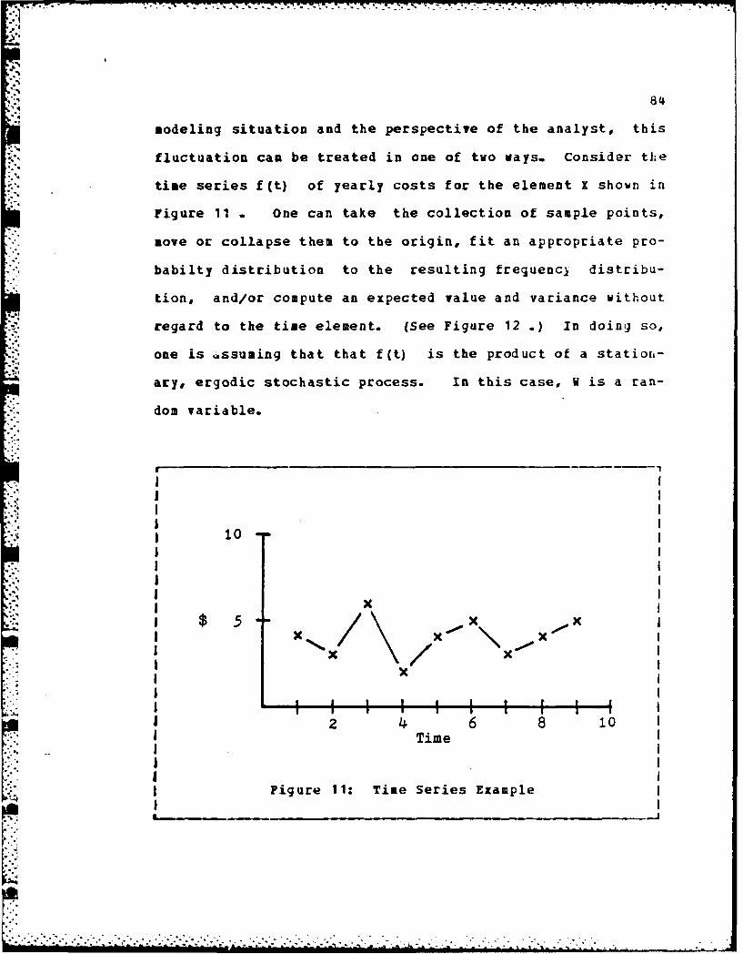
'984
modeling situation and the perspective of the analyst, this
fluctuation can be treated in one of two ways. Consider the
-' time series f(t) of yearly costs for the element X shown in
Figure 11 * One can take the collection of sample points,
*" move or collapse them to the origin, fit an appropriate pro-
babilty distribution to the resulting frequencl distribu-
tion, and/or compute an expected value and variance without
regard to the time element. (See Figure 12 .) In doing so,
one is .ssuaing that that f(t) is the product of a station-
ary, ergodic stochastic process. In this case, W is a ran-
dom variable.
10 -
X
- X XX I
x
I I I I I Ii2 4 6 8 10
Time
Figure 11: Time Series Example
""' "" " " " '""-"'" ' '"" " " " " '" ' " """ ' '"" " "" ' "-- - , .,... .. :...... ,. _ " "' " " ' ,,,_.,'"' ,. _ _ ...p..

85
"10
- --
X X
Time
Figure 12: Time Series Collapsed
By the same token, the value of Change (Z) is not known
with certainty. Thus it also can* be regarded as a randomt
variable from some possibly an-known distribution. Using the
sums and products of random variables approach, and assuming
V and Z are independent, the expected value and variance of
the cost element X are
E[X] = E[V],E[Z] (46)
Var[l] = Var[Vl Var[z ] (47)
Note that the variance is a sum for both the sum and differ-
ence of tvo random variables. In terms of transforms, thedistribution of I can be expressed as a convolution integral
and applying Borells theorem,
I I"
I "I
86
L[f(X) ] = L[g(W) ] L[h(Z) ] (48)
where L[g(W) ] and L[h(Z)] are the Laplace transforms of the
distributions of V and Z respectively. In the case of a
difference, the complex variable s in L[h(Z)] is replaced by
minus s (-s).
As the second alternative in treating the time series,
one can look at the data points as a single realization of
the time series (and the only realization available) and
compute a separate cost for the element X for each year.
This treatment is applicable if the time series appears to
be changing over time; that is, a positive or negative trend
is apparent. In the absence of any further information, the
value of W for any year j is regarded as a constant. Thus,
Xj = VjZj (49)
The change in the cost element in year j, Zj is still a
random quantity. Thus, the expected value and variance of Xj
are, respectively
E[Xj] = Vj&E[Zj] (50)
Var[Xj] = Var[Zj] (51)
In transform domain, the Laplace transform of the distribu-
tion of Xj is
L[f(X( ] = e-SWj L[ h (Z j) ] (52)
Again, in the case of a difference, the complex variaile s
in L[h(Z)] is replaced by minas s (-s).

87
Parametric estimation presents a sore complex situation
due to the complexity of some of the CERs used. CERs con-
sidered here are of two types: factor based and regression
analysis based. The factor based CERs are essentially sim-
ple sums and products of random variables. As an example,
consider a CER where fuel cost per year is estimated ty mul-
tiplying flying hours per year by fuel cost per flying hour
or
FC FHx CH (53)
vhere
FC = fuel cost per year
FH = flying hours per year
CFH fuel cost per flying hour
regarding FH and CFH as random variables, FC is then the
product of two random variables. FH and CFH are factors.
Thus, in general
qXi 7r_ Fk ' =11...,13 (54)
where q is the number of factors in the product for the ith
cost element. Cost factors may also be added'?. Thus, a
CER may appear as
Xi = e i1,...,m (55)k=1
17 In cost estimation, factors are not defined in the alge-braic sense of quantities multiplied together.
' '..,.. . . . . . . . . . . . . . . . . . ..

88
where q is the number of terms in the sun. Multiplicative
and additive factors may appear in the same CER. To proper-
ly evaluate these CERs* the reader is referred to the sec-
tions on suns and products of random variables and trans-
forms.
Before proceeding with regression analysis based CERs, d
word of caution is in order. Consider the two alternative
CERs
Example 1 Y = 4X (56)
and
Example 2 Y = X+X+X+X (57)
Although they may appear to be the same at first glance,
they are not. The expected values of Examples 1 and 2 re-
spectively are
E[Y] = 4E[X] (58)
and
E[Y,] = E[=X].E(1JE(XJ.E[ 1 42[Z1 (59)
which reinforces the notion that the models are the same,
but the variences of Examples 1 and 2 respectively are
Var[Y] = , 2 VartX] 16Var[l] (60)
and
Var[YI] = Var[ ]+Var[ ]+Var[X]+Var[(] = 4Var[X) (61)
Upon examination of the variances, it is clear that they are
not the same model. The point of this demonstration is to
reinforce the principle that models should be a reflection
[. "• ° . . . . . . :. . . . . . . . . .. . . . . . .
- i - ' ,lu.- - - - - - . • . .- .mm - -' a; . - --.

89
of reality. If the reality of the situation suggests Exax-
ple 1, then use it. But if reality suggests Example 2, do
not use Example 1 as a shortcut for representing a Example 2
situat ion.
Many CERs are derived by fitting curves to historical
data. This is normally done by the method of least squares,
which may be linear or nonlinear. Once the regression equa-
tion is accepted, the coefficients in that equation (which
are really estimates themselves) are taken as constants and
the independent variables in the equation are then treated
as random variables.
Consider then a model of the general form
X = f(F, F 2 ,.o.IFq) (62)
where f is a function of the factors Fl,...,Fq . If FjF 2
-.. ,Fq are random variables, X is also a random variable!
with expected value
E[X] = E[f(FIF 2 ,...,Fq) 3 (63)
and variance
Var[X] = Var[f(FIF 2 ,...#w Fq) ] (i4)
The problem is then to find the expected value and varianc.
of f, which may be a rather complicated function.
Two commonly used forms for the function f areForm 1 f(Fl) = a+bFE (65)
and
Form 2 f(FF 2,..Fq = bFElFE2...,q (66)
1 2 q

* 90
where a, b. and El... Eq are parameters. One can represent
the function f by a Taylor series expansion about the point
= 4 where 4iis the expected value of Fi and
apply equations (10) and (11) to approximate the expected
* value and variance of the function.
Using transforms, evaluation of Form 2 is quite direct
but rather involved in the case of Form 1, which can be- Le-
written as
f(Fl) =a4Z (67)
where
Z = bF~1
The product bFE1 is evaluated using the n ellin transform1.
which is
ME g(Z) J=bs1 F(lsFl1 (63)
In words, the Iellin transform of the distribution of Z,
9(z)#, is bs-1 times the !ellin transform of the d-istribution
of F, with (Els-E1 +1) substituted for the complex variable
IS. This transform MI(g (z) ] is then inverted yielding g (z).
The Laplace transform is then used to evaluate f(F1) giving
L( h(f (F1)) e -sa.(Z) 1(69)
* The inversion process then yields the distribution hif (F1))
which is zero to the left of the point f(Fj) =a
Form 2 is addressed using only the Mellin transform which
is
ME h (f (F j#F 2 eeFqfJ b -MF(21- +1 2 s +
MF [( -q~ (70)q qEl
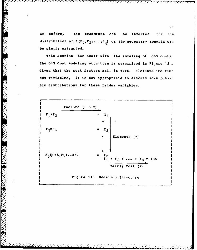
91
As before, the transform can be inverted for the
distribution of f(F1eF2,...Fq) or the necessary moments can
be simply extracted.
This section has dealt with the modeling of O&S cnsts.
The OSS cost modeling structure is summarized in Figure 13
Given that the cost factors and, in turn, elements are ran-
dom variables, it is now appropriate to discuss some ossi-
ble distributions for these random variables.
-, .- I
I-'. ! Factors ( & x)
.iFI+F 2 X1
+
.F 3xF =X 2
I .4. Elements ( )
.4, +
F 5F6 F7 F8 .*Fq _. .j= OY1 + I2 + • In TOS
Yearly Cost (*)
% Figure 13: Modeling Structure
i%.
%'
92
3.3 ZR2. BIIT D..S Rn zBU X o.TN.
a variety of probability distributions have been applied in
cost modeling. Typically, the true distribution is unknown,
necessitating some assumptions on the part of the analyst.
One such assumption used in this research is that cost is
continuous and that the factors used in arriving at cost are
also continuous. In some cases, a continuous distribution
may be used to approximate what is usually a discrete dis-
tribution. One example is manpower. In actual practice,
one cannot meaningfully assign half a person to a particular
base or weapons system, but it is felt that such minor dis-
tortion, when viewing the entire OS cost picture, vili be
slight and, thus, can be reasonably disregarded. At this
point, it seems reasonable to establish a set of criteria
against which various candidate distributions can be judged.
Wilder and Black [89:195) suggest the following:
1. Finite ends
2. Not necessarily symmetric
3. Unimodal
4. Computationally simple
To this list can be added the following:
1. Wide variety of shaDes
2. Parameters easily determined
3. Conducive to subjective input

93
Not all the proposed distributions meet all of these cri-
teria. Since little data and information exists regarding
the actual distribution of O&S cost factors and elements, it
is often necessary for the analyst to sake assumptions re-
garding the distribution to be used. Such assumptions
should reflect the reality of the modeling situation and
make good intuitive sense. The choice will often be driven
by the information available. For instance, if one cani only
reasonably determine the first two moments, it does not seem
reasonable to use a distribution requiring, say, four mo-
ments for parameterization.
In many instances,the parameter values of the various
distributians just be determined from subjective input.
This is particularly true for new proposed systems where
substantive data is lacking. Post often these subjective
inputs are based on the opinion of experts, either collec-
tively or individually. In collecting such data, it is de-
sirable to keep the information required simple and to a
minimum. This forces the analyst to make some basic assump-
tions and, in some cases, to use some simplifying approxima-
tions. The most basic assumption is which distribution
should be used to model a certain factor, cost element, or
- situation. Once the distribution has been chosen, the ana-
lyst must obtain nme i' 4rmation regarding the factor or
cost element. In keeping the information on the cost factor
St
a,.

94
to a minimum, it wili be assumed that the expert can furnish
* only a low estimate (L), most likely estimate (M), and high
estimate (H). With this limited information in hand, the
analyst must then determine applicable distribution parame-
ter values.
six candidate distributions are discussed in this sec-
tion. This is by no means an exhaustive list, but these
distributions have found past application in cost analysis.
In most cases, however, they do not meet all the criteria
listed above. These distributions are the normal, log nor-
mal, triangular, beta, rectangular, and gamma. The discrete
Poisson distribution is also presented for use in computing
random sums of random variables.
3.3.1 IThe lormal Distribution
The normal is perhaps the best known and most used distribu-
tion. It has found wide application and applies when small
deviations from the mean are more frequent than large devia-
tions and when positive and negative deviations of the same
size are equally likely. This distribution is fully parame-
terized in terms of its mean and variance.
Mathematically, the normal probability distribution is
defined by the probability density function
1 2f~x M V2-c 17 exp[- 1/2[ (x- )/orJ
-00 rb X 0 (71)
where
...... .... .

:-4
-7i
= a constant (approximately 3.11416)
4 = expected value of x
a = standard deviation of x
One specific variation of the normal distribution, the
standardized normal is of particular interest. This varia-
tion, often referred to as the unit normal or z distribu-
tion, has a mean of zero and a variance of one and is relat-
ed to the normal through the standardization formula
z = (W-p.)/a (72)
Several cautions are in order regarding the use of this
distribution. First, unfortunately, a closed form expres-
sion of the cumulative distribution function18 does not ex-
ist and its evaluation can only be obtained through apFroxi-
mate numerical procedures. Second, it fails to meet several
of the criteria set forth earlier. It does not have finite
ends. In using this distribtioa, one is automatically as-
suming that costs can go to infinity in both the positive
and negative directions. Also, the distribution is symme-
tric about the mean, thus severely limiting the shapes it
can attain.
In spite of its deficiencies, in the absence of any real
indication to the contrary, this may be the best distribu-
tion to use in cost analysis, partcularly when one is work-
1 The cumulative distribution function is defined as F(X) =
J f(t) dt• ['---0
96
ing with the sums and products of random variables and mean
and variance is all that is known.
In the case of the normal distribution, parameter values
determined from subjective input must be approximated. An
approximation can be made based on the fact that ninety-nine
percent the observations fall within plus or minus three
standard deviations of the mean. Thus, knowledge of L and H
is all that is required. If one can obtain a range, L to H,
of the random variable, then (L+H)/2 is the meanig and
(H-L)/6 is the approximate standard deviation.
Before proceeding with this discussion of probability
distributions, a few words concerning the central limit the-
orem are in order.
3.3.1.1 Central Limit Theorem
It can be shown that the sums of independent normally dis-
tributed random variables are themselves normally distribut-
ed and, that even if the random variables are not normally
distributed, the distribution of the sum still tends to be
normal. In a general form, relaxing the identically dis-
tributed requirement, Hillier and Lieberman (47:366] state
that if the random variables X,...,0 Xn are independent with
means and variances ci2 t. . ,O 2 respectively, then
19 For the normal distribution, the mean and mode or mostlikely are the same. The mean computed here can be coc-pared to the 8 obtained subjectively in evaluating theappropriateness normality assumption.

97
the random variable Zn,Zn= (nZi-rEi)/ If;5 12n
(3n n
under certain regularity conditions is approximately normal-
ly distributed with zero mean and unit variance in the sense
that
bli P(Zns b) LJ (2 [ 1 exp(-Y2/2) dY (74)n- 00
A number of central limit theorems for dependent random
variables have been developed, although it is not possible
to state a simple general result in this case (46:26-27].
In spite of the generalities of the central limit theo-
rem, normality may or may not be a good representation of
the sums of random variables involved in O&S costing. Ac-
cording to McNichols [71:119], the applicability of normali-
ty will depend on the number of variables in the sum, the
relative shapes and spread of the distributions, and the de-
gree of dependency, if any. He concludes that arbitrarily
restricting the distribution of the sum to be normal could
grossly understate the true risk. However, in the absence
of more definitive information, the assumption of normality
is both logical and warrented.

98
3-3.2 The &qg Lo !ll Distribution
The log normal distribution offers some improvement over the
normal in that it has a finite left tail anchored at the or-
igin and an infinite right tail, yet, it is not quite as
easily handled and is limited in shape. The log normal den-
sity function is
f(t) = (a t V2 -1 exp[-1/21(ln t-.li)/5 2] U
t 0 (75)
where and a are parameters such that -c < and In
stands for natural logarithm.
If a random variable X is defined as X In t, then X is
normally distributed with mean U and standard deviaticn c5.
Using this substitution and the normal distribution, it can
be shown that the mean and variance of the log normal dis-
tribution are
Eftj = exp[ 4+,.2/2] (76)
and
Var[t] = expf2u+c 2 ](exp[a2 -1 1 (77)
Values for the parameters U and a are determined from sub-
jective input in the same way that these parameters are de-
termined for the normal distribution.
:"..-". --.- .----.-.-..-...-.......-.-........... ..... ... .

99
3.3.3 The triangular jistributio
The triangular distribution is relatively simple and is com-
pletely parameterized with knowledge of only three points.
The probability density function is given by{2(x-a) ]/[ (b-a) (m-a)] if a s x m
f(Z) = (7b)
2(b-x) ]/C (b-a) (b-m)] if a r. x b
where
a = lower limit (a 0)
a = most likely value (mode)
b = high, limit
This distribution has all the properties listed. It is
bounded and incorporates skewness. Further, it appears to
be any easy concept to visualize and understand, especially
for those not familiar with statistics [89:195].
The lone drawback to this distribution is the- lack of
smoothness at the point x = m. This necessitates the Lreak-
ing of the transforms for the triangular distribution into
two parts. That is,
L[f(x) e e'Xf (i) dx +f e-SXf2c) dx (79)a M
and
(M ) f W s1I Z dir + 1 S-l 1 2 (x) x(0m m
where
f (z) = [2(x-a) V/ (b-a) (a-a) ]

100
f2(") [2(b-xj ]/[ (b-a) (b-m) J
For this distribution, knowledge of L, R, and H complete-
ly defines the distribution. Just set L = a, M = a, and H -
b.
3.3.4 The Beta Distribution
The generalized beta distribution, along with its special
cases, is probably the most used distribution in the area of
stochastLc cost estimation. It offers great versatility in
terms of location and shape. The beta distibution probabil-ity density function defined on the interval [a,a~b] is
f (x) = io+ )/Ic)Io)b) ((x-a)/b) -i
(1- (x-a)/1b) (81)
where
](a= the gamma function y exp[-y] dy0
and
a s xs ab >
The parameter a is the low value, b the range, and a+b the
high value of the distribution. The parameters a and 5 are
shape parameters. A standardized version of the beta dis-
tribution2o over the interval [0,1] is obtained by the
transformation y = (x-a)/b giving
f(y) [y 1YS- I/B (a, 0 (82)
20 Sometimes referred to as a Type I beta as opposed to thegeneralized Type I1.
4 , . . .. . . . .. . . . - . . . . .. 4 44 .

101
where
B (X,) $ 1 1 a11(l...) 0 1 dy (FIz)'(3)V (X+O)
The cumulative distribution function of the standardized
beta random variable is commonly called the incomplete B-
function denoted by
FMy 0=1 (tll-t) 0-1 ]/Bl(cx,) dt (83)
0
The beta distribution is particularly appealing to some
in that it sets upper and lower limits on the cost factors
and elements, it can have any left or right skewness, and it
assumes many shapes.
Parameter estimation for the beta distribution is some-
vhat more involved since there are more parameters to esti-
mate. Several subjective parameter estimation techniques
have been proposed. The most well known is that developed
as a part of the Program Evaluation and Review Technique
(PERT). First used to model the distribution of activity
durations in networks, the originators assumed that a low
(L), high (H), and most likely (M) value for the time of
each activity. Then setting the parameters a and b to a = L-
and b = H-L, the mean and variance are approximated by
I (L+*H&)/6 (84)
S2 = (H-L) 2/36 (85)
.......................

102
Since the original PERT proposal, it has been shown that
this approximation corresponds to only three a,O combina-
tions, thus severely limiting the shape and versatility of
the distribution. The user should be aware of these limita-
tions and possible errors prior to using the PERT approach.
As an alternative to the PERT approach, the procedure
presented here was first introduced by Donaldson [ 30] and
later modified by Coon [21]. It produces a more general
class of beta distribution than the PERT, but assumes that
th-e distribution is tangential to the horizontal axis at
each end This has the effect of limiLing a and to values
greater than or equal to two.
From the previous discussion of the beta distribution and
using the three estimates (L, N, and H), it can be shown
that
L = low = a (86)
H = high a+b (87)
M = mode = [a($-1)+(a'b) (a-1) ]/(a+0-2) (88)
Substituting the above estimates and rearranging,
(89)
This result is an 'assymetry' measure. The remainder of the
derivation by Donaldson and Coon is somewhat involved, but
the decision rules can be summarized as follows:
if (H-M) > (M-L) set a=2 and 0=(H-N)/(N-L).1
if (H-L) > (H-N) set 0=2 and C=(M-L)/(H-M)+I (90)
otherwise set a=0=2

103
Although this procedure does not allow a full range of the
beta distribution, Donaldson has shown that it allows skew
to range from -1.14 to *1.414, while the PERT is valid at
only three values, -0.707, +0.7070 and 0.0.
As another special case of the beta distribution, consii-
er the rectangular distribution. It occurs when a and 0 are
one.
3.3.4.1 The Rectangular Distribution
Thb rectangular distribution, often confused with the uni-
form distribution, is a continuous probability distribution
which gives the probability that a sample value will be
within a given interval when probability is directly propor-
tional to the length of the interval. Mathematically, the
rectangular distriution is defined by the probability den-
sity function
f(z) = 1/b , 05 axra+b (91)
While this distribution does meet most of the above cri-
teria, it is severely restricted with regard to shape. It
is, however, easily parameterized with knowledge of L and H!
where b = H-L
S
-p

3.3.5 Thj Gana Dis&ibutio1
The gamma distribution, although well known and widely used,
has found limited application in the field of cost analysis.
[ts probability density function is of the form
f(x) = [ - x-k a -92exp[ )xk)
with
cxOk > 0 xz k
where
= shape parameter
= scale parameter
k = location parameter
This distribution is characterized by a finite lower tail
and infinite upper tail. gith k equal to zero, the lower
tail is anchored at the origin indicating that the lower
bound On cost is zero and the upper bound is infinity. Such
a distribution could have a rather large variance, but may
be indicative of the true risk involved in some programs.
Even if k is not zero, this distribution reflects the risk
of escalating costs and budget overruns which seem to be so
common in weapons system acquisition and support. Others
argue that there is an upper limit on affordability, but
such a limit is neither clearly defined nor does it seem to
be stationary.
In reference to the previously defined criteria, this
distribution meets all with the exception noted above. It
• -. .. . , • . . • - • .- , . .- ,. - -. . .. . _, .' :.. . -..... . _.-.,
105
should be noted, however, that the gamma distribution is
". limited to positive skewness.
Parameter estimation for the gamma distribution suffers
*i the same general limitations as the beta distribution due to
the form of the incomplete Gamma function. Therefore, ap-
proximations for the mean and variance vili be used to esti-
mate the parameters. The procedure presented was developed
by Perry and Greig [86] and requires that L and H be rede-
fined as L6 and H6 where L6 is a low estimate such that the
probability of anteceding it is 6 and H6 is a high estimate
such that the probability of exceeding it is also 5. With
8=.05, Perry and Greig have shown that
' (L6+.95M+H 6)/2.95 (93)
and
a2 " ((H6-L6)/3.25)2 (94)
From the properties of the gamma distribution, it can be
shown that
= mean = B+k (95)
a2 variance = a02 (96)
R = node = $(a-1)+k (97)
Subtracting (97) from (95)
4-H (98)
where the value of p is determined from (93) above. Equa-
tion (96), with a2 determined from equation (94), is then
used to solve for a. Vith a and 8 both known, equation (95)
"4 a" - , : ' , ,: : : :: : :":: . ;:.;,. .. . . .. . --_;,;:L L _:_- -

.7o 7
106
is them used to solve for k. Thus, the gamma distribution
parameters can be determined using the three subjective in-
puts.
3.3. 6 fe Poissom Distribution
Before concluding this section, it might be helpful to in-
clude a discrete distribution to be used in addressing the
random sums of random variables. For this purpose, th-.
Poisson distribution has been selected. Its probability
mass function is
p(n) = An/n! e - , n=,.-..,OO (99)
where A is the lone parameter equal to the mean and variance
of the distribution.
Haight (42:12] has shown that the Poisson distribution
has a unique mode satisfying the relationship
X- 1 :5 mode :g X (100)
Therefore, one can use the subjective estimate of the mode,
M, as an approximation for A. If the analysis is sensitive
to this parameter, both extremes in (100) can be used.
Table 10 summarizes the results of this section and gives
some pertinent information relating to transforms.
-... . . .. . .... ......... ..... .. . . ... o.

107
TABLE 10
Probability Distribution Summary
mI "
IV
Alis I
aArai
10.I
I -1
-; _ J

108
3.4 "tiiNINiG TBRE RISK AVALYSIS
Once the risk analysis has been accomplished, the results
must be meaningfully conveyed to decision makers. In light
of the objections stated in Chapter 1, this is no easy task.
In meeting the needs of decision makers, the information
presented must be clear, concise, easily understood and rel-
evant to the decision.
Perhaps, the most simple and direct statement of risk is
variance. Unfortunately, the mere expression of variance
has little meaning or intuitive appeal to most decision mak-
ers. Numbers must be coupled with a visual sense of magni-
tude. One way to do this is through a mean-variance plot.
In comparing alternatives using a mean-variance plot, the
mean is plotted on the horizontal axis and the variance on
the vertical axis. (See Figure 14 .) Each alternative is
represented by a point on the plot. In comparing alterna-
tives, low mean cost is preferred to high and low variance
(risk) is also preferred to high. Thus, in the case of al-
ternatives I and C,. both with equal mean, A is preferred to
C as it has least variance. Likewise, in the case of alter-
natives A and B, both with equal variance, A is preferred to
a since it has the lower mean cost. Therefore, it can be
said that A is preferred to all other alternatives including
D. A problem of choice occurs if B and C are the only com-
peting options. Alternative B has lover variance but higher

109
mean than C. This is Ehere decision makers' preference for
risk invades the decision process. A risk averse person way
choose B, while a risk seeking person may choose C. The de-
cision may also be influenced by the distance which sepa-
rates the points on the plot. As a variation, the mode can
be substituted for the mean and standard deviation for vari-
ance.
e D
x x
Variance
A Bx x
Mean I
Figure 14: Mean-Variance Plot
Tolerance intervals can also be used in presenting the
risk analysis results. A statistical tolerance interval is
an interval within which one can state with a given prob-
ability of being correct that at least a prespecified pro-
portion of a distribution is located [41:77]. The end
4h
. .. . . .. .. .... |" " ""." ' ' ' "
' ' l 'I , . .

110
points of such intervals are called tolerance limits. Tol-
erance intervals are not to be confused with confidence in-
tervals A confidence interval defines limits which will
cover or contain a population parameter with a certain con-
fidence- Although this difference may seem subtle, toler-
ance intervals and confidence intervals answer quite differ-
ent questions.
In order to apply tolerance limits all explainable causes
of variability must be detected and eliminated and certain
assumptions must be made concerning the population under
study. If one assumes that the parent population is normal-
ly distributed with known sample mean and variance, the tol-
erance limits take the form
K Ks (101)
with K chosen so that one may expect these limits to inclulr
at least P percent of the population at some prescribed
probability level Y. Standard deviation is represeiated by
s. Table 11 lists K factors for various values of P assum-
ing an infinite sample size and point nine five (.95) prob-
ability level [83:103]. The reader will note that with an
infinite sample size the K factors are the same as the stan-
dard normal random variable.
Computing, plotting, ard using the cumulative distribu-
tion function is also a convenient and descriptive way of
presenting a risk analysis. By definition, the cumulative
-o*** ~

''~' - .-v--- . . . . . . . .. . - - .. '
111
". TABLE 11
Two-Sided Tolerance Factors
I P K
" .75 1.150
.-. 90 1.645
I .95 1.960
.99 2.576
distribution function is a function that describes the prob-
ability that the random variable X will take on a value less
than or equal to a prespecified value I within its domain.
Mathematically, this is
F(b) = P(Xs b) =J f(1) dX (102)
where f(X) is the probability density function.
Thus, the cumulative distribution function allows the an-
alyst to make probability statements regarding costs of
weapons systems. For instance, refering to Figure 15 , it
can be said that there is a probability of .75 that the cost
will be less than or equal to S5.1 million or that there is
a .50 probability that it will be between S2.8 and $5.1 mil-
lion. Competing systems can also be compared by plotting
their cumulative distributions on the same azis.
* . ... ,. * . . . .

112
11.00 1
I I(X .50
I .25
1 2 3 456 789190 1
I $ Millions
I Figure 15: cumulative Distrbution Function Plot
I ( SI K.0I13
Plth floatingeoa bar graph To cosruct the Fgrph tak The
= 90(13
graph cam be enhanced by indicating the mean and modal cost
for each alternativa. This presentation indicates the vari-

113
ability plus the location of the mean and mode for decision
makers.
10
I A AI 8 2
I I
Mea Mod
i lles os 5 bepeetdtIeiio aesi en
infl infrmaiv va. Tenx hpe eosrtsai
presents~~ exmlso h aeildsusdi hscatr

m-.1
Chapter IT
APPLICATIONS
The purpose of this chapter is to demonstrate some applica-
tions of the theoretical aspects of risk analysis presentei
in the previous chapter. once again the emphasis is on op-
-'erating and support (OSS) costs. The specific modeling
methods and probability distributions used are for illustra-
tive purposes only and are not intended to imply that others
could not be used. The objective is to demonstrate as many
of the techniques presented iba the previous chapter as pos-
sible within a given, typical 08S cost analysis scenario.
4.1 fiEMU~L~ APPROACH
A four step approach is recommended in performing any cost
risk analysis. These steps include:
1. Determine most likely point estimate
2. Perform preliminary risk analysis on cost drivers
3. Accomplish indepth risk analysis where warranted
!-
4. Do sensitivity analysis
The first step is a preliinary analysis to determine the
cost drivers and satisfy the need for a point estimate.
114-1
This estimate should be based on the most likely cost ofI
each element and need only be done for a single. typical
year in order to identify the cost drivers. In doing the
point estimate, the analyst most determine the appropriate
estimating technique to be used for each cost element.
With the cost drivers identified, the next step is to
perform a preliminary risk analysis. Additional information
is gathered on the parameters relating to the cost drivers
which will permit the analyst to do a preliminary risk anal-
ysis. This analysis is done only on the cost drivers or
cost elements where risk is of concern and should be done
using the sums and products of random variables methol.
These results will indicate if further, indepth risk analy-
sis is necessary.
Indepth risk analysis is then performed on parameters or
cost elements which warrant such attention. -This *micro-
scopic' analysis can be done using transforms to determine
the type aad/or moments of the distributions involved. In-
formation gleaned from this step can be used to update an"
refine the preliminary risk analysis.
The last step is a sensitivity analysis on those parame-
ters or cost elements which are shown to be quite sensitive
to the analysis.
As a modified approach, the analyst may determine the
4 cost drivers a priori either from personal experience or

- - . -. - - - - . - -7. -
116
from the program scenario. In this way, data needed for the ,
risk analysis can be collected along with ths information
necessary to do the initial point estimate. This modified
approach may save some time and effort. For new systems,
the cost drivers can often be identified by examining costs
and cost related parameters on existing, related systems.
Since such of the data relating to new, perspective sys-
tems is based on expert opinion, a few words and cautions on
collecting such data are now in order.
4.2 SUBJECTIVE INPUTS
Mlost experts, when making subjective estimates, attempt to
compare the situation confronting them to past, relatel
situations which they have encountered. This is done di-
rectly or indirectly; overtly or covertly. Some are better
at using their experience than others, not necessarily be-
cause their experience is of a higher quality Out because of
*the-flexibility they display in using their experience, it
is the task of the analyst to lend assistance and direction
in this process.
Probably the most difficult task confronting experts is
distinguishing between what they want to happen and what
they think will actually happen. Often the expert has a
vested interest in the area for which information is sought
and may assume somewhat of an advocate role. If the expert

117
is personally involved with a program, that person will nat-
urally want the program to succeed and, unless great care is
shown, there is a tendency to be less objective than other-
wise. Further, if the estimate provided will also be used
as a yardstick against which the expert's performance is
measured then there is a natural tendency to be conserva-
tive.
Often a group, rather than a single expert, is used. it
can be argued that this is one way of overcoming some of the
previously mentioned biases. The problem which then arises
is that of combining a number of different estimates into d
single estimate. Should an average be used or should mor2
weight be given to the estimates of more knowledgeatle ex-
perts? If there is a group discussion to resolve differenc-
es, there is a danger of the group being unduly influencel
by one or two dominant personalities.
One approach to group forecasting which has received a
great deal of attention-in the literature is the Delphi
technique. This technique provides a means to incorporate
feedback into the estimating process. It involves interro-
gating experts by means of a sequence of questionaires; the
first of which is an independent input from each expert.
These inputs are then aggregated and a summary is then pre-
sented to each expert who is then asked to reconsider the
previous, independent input in light of the new information
. .i
.%• 1 18
contained in the summary. The process is then repeated un-
til consensus is achieved. Thus, through this technique,
personal contact and domination by forceful personalities is
avoided.
Apart from enabling a more meaningful analysis, estimat-
ing risk can have distinct advantages. Experts are often
far more willing to make uncertainty estimates than point
estimates since point estimates may seem like a personal
commitment on the part of the experts.
•In gathering subjective estimates, the problem and infor-
mation needed must be clearly defined. All possible biases
should be eliminated. To avoid anchoring, the experts' at-
tention should be initially directed toward the extreme val-
ues. Thus, the high and low estimates should be obtained
before the the most likely estimate. The analyst must first
allow the expert to appreciate the full range of risk.
Questions such as, 'How bad could the variable get?' and
'Could the value in fact turn out to be better than antici-
pated?' should be asked. A dialogue between the analyst and
expert must be established with the analyst being cdreful
not to lead the expert.
Once the high and low values have been reasonably deter-
mined, the expert is asked to give a best guess or most
likely value for the variable. As a final test, the analyst
should assess the expert's willingness to place a bet on the
119
value of the variable being greater than the high or less
than the low estimate. This often leads to a revision of
the estimates.
The gathering of subjective estimates is an art ani re-
quires the analyst to use sound judgement, ingenuity, per-
severence, and good human relations.
4.3 fLH SCENARIO
The Air Force is conducting preliminary cost studies on the
Follow-on-Fighter (FoF) which vill augment the current fleet
of F-15 and F-16 aircraft beginning in 1995. The Foe is to
be used in an air superiority role, thereby freeing current
aircraft for interdiction and close air support roles.
Three squadrons of twenty-four aircraft each will be re-
quired with all production to take place in 1995. The oper-
ational life of this aircraft is expected to be only six
years due to the introduction of the Space Defense System,
which will be operational in the year 2000.
Industry has proposed two versions of the FoF: the XF-I
and the XF-2. The XF-I will be a single engine, single seat
aircraft, whereas, the IF-2 will be dual engine, dual seat.
Both will have the same operational capability, but with
several additional basic differences. Due to weight and
speed specifications, it will be necessary to build the XF-i
airframe from new, light weight, composite materials. The
" . . '., ,o? o .. i. . . " i. . .< . i i .'. ..... . .
120
development and production of these new materials is consid-
ered to be high risk. In contrast, the XF-2 will have a
more conventional construction, but will exceed the XF-1 in
both size and weight.
The XF-1 will be powered by the new astrojet engine which
will use jet fuel impregnated with ether. The ether impreq-
nated fuel will produce more thrust# but, on the negative
side, more heat, than conventional fuel. Due to the unpro-
ven technology, the astrojet engine is also considered to be
high risk. The IF-2 will be powered by conventional jet en-
gines.
The IF-i avionics package is also a concern. Due to lim-
itations on its single crewperson, the XF-i avionics must
operate automatically, as opposed to the more mdnual XF-2
". avionics. Due to the automated features, the XF-1 avionics
will challenge the state of the art and, therefore, presents
a high risk.
The-FoF OS cost estimate is to be done in accordance
with the CAIG-approved OS cost element structure (CES) and
is to include a risk analysis.
'K

121
4.4 MOST LIKELY POINT ESTIMATE
As the first step in the analysis, a preliminary point esti-
mate using most likely values and appropriate estimating
technigues was accomplished. This is a single year steady
state estimate. The results of this analysis are presentel
in Table 12 -
TABLE 12
FoF Preliminary Cost Analysis
$millions FY83
Category XF-I XF-2
Unit Mission Personnel 31.195 34.111
Unit Level Consumption 35.123 39.233 1
Depot Level Maintenance 18.282 17.947
Sustaining Investment 11.066 14.798
Installation Suport Personnel 7.450 6.88,)
Indirect Personnel Support 8.220 8.240
Depot Non-Maintenance 2.080 2.164 1
Personnel Acquisition 8 Training .000 .000
Total 113.416 123.373

122
From Table 12, it is readily apparent that Unit Mission
Personnel, Unit Level Consumption, Depot Level Maintenance,
and Sustaininy Investment are the FoF cost drivers. These
four elements alone account for about eighty-five percent of
the total 0SS cost.
Upon closer examimnation, the analyst identified mainte-
nance personnel as d subelement under Unit Mission Personnel
for risk analysis, particularly in the case of the XF-i with
its new engine and avionics. Fuel consumption is the major
contributor to Unit Level Consumption and is therefore iden-
tified for risk analysis. Depot Maintenance, although dif-
ficult to estimate, is the third highest cost element for
both aircraft and is, therefore, subject to risk analysis.
Under Sustaining Investment, replenishment spares is the ma-
jor contributor to cost, particularly in the areas of avio.-
ics and engines. Therefore, these areas deserve special at-
tention.
The costs identified for risk analysis are consistent
with the scenario and represent most of the risk in this nev
program. They account for sixty-nine percent and seventy-
five percent of the total support cost for the XE-1 and XF-2
respectively.

123
4.5 PREIMN.ARY RISK ANALYSIS
4.5.1 learlj Cost Copuaion
4.5.1.1 Maintenance Personnel
The analyst has determined that analogy using an F-16 base-
line for the XF-i and an F-15 baseline for the XF-2 is tho
most reasonable approach to maintenance perscnnel cost risk
analysis. The first task is then to determine the number o.
personnel necessary to support the FoF. Table 13 lists the
necessary information.
TABLE 13
Maintenance Personnel Requirements
F-16 XF-1Baseline Additions
Total 1728 35
Avionics 197 30
Engines 118 5
F-15 XF-2., Baseline Additions
""Total 1774 10
Avionics 251 7
Engines 192 3
Baseline Source: Headquarters, Tactical Air Command
Io_____
b---------. ..-

124
In consulting with Air Force personnel experts regarding
the FoF additional maintenance personnel, the analyst sur-
mizes that the additional personnel follow a Poisson distri-
bution with mean, mode, and variance equal to 35 and 10 for
the IF-1 and XF-2 respectively. Thus, using an adaptation
of equation (49), the number of maintenance personnel (1,P)
is represented by the equation
MP = Base 4 Change = + 4 Z (104)
and
E[MP] = 9 + E[Z] (105)
Var[MP] = Var[Z] (106)
These calculations are summarized in Table 14 o
TABLE 14
Maintenance Personnel Calculation Summary
XF-1 .. XF-2
E[ MP] 1763 1784
Var[MP] 35 10
The next step is to determine the pay for these mainte-
nance personnel, which is summarized in Table 15
Nov combining the results of Tables 14 and 15 and using
the additive model where the number of terms in the sum is a
p - .

ri : r .- . • -.. . -. . . . .. .. , _- . , . o. . . • ,- - . . -
125
TABLE 15
Maintenance Personnel Payr
Composite Pay Members Fraction IGrade FY83a in Gradeb of Force
E-9 $35,285 4,749 .°01
E-8 29,859 9,478 .02
E-7 25,756 34,402 .08
E-6 21,876 53,344 .12
E-5 18,346 102,261 .22
E-4 15,497 102,269 .22
E-3 12,618 120,082 .27
9--2 11,4460 26,244 .06
1.00
E[PAY] = $17,513
Var[PAY] = 23,703,700
a - Source: AFR 173-13b - Source: Air Force Magazine 66 (May 1983): 165
Note: E[ ] = IP(Y)
C IjVar[ I] =2.(Y-ELYJJ- P (Y)
random variable, application of equations (27) and (28)
yield the results shown in Table 16 with detailed calcula-

126
tions for the XF-1 contained in Appendix E. The symbol 'SO'
stands for standard deviation which is, of course, the
square root of the variance. In later parts of the paper,
the symbol oE'E is used to represent scientific notation and
means to multiply the number preceeding the 'EE' by ten to
the power of the number following the 'ER'.
I-- I
TABLE 16
Maintenance Personnel Yearly Pay Summary
$millions FY83
XF-i XF-2
E[ X] 30.875 31.243
SD[0. 1 0.229 0.213 1
4.5.1.2 Fuel
The analyst chose the factor based cost estimating relatio.-
ship (CER) tor fuel from the Logistics Support Cost (LSC)
Model [65] to estimate the FoF fuel consumption. The CER,
in a slightly simplified form, is
Z = EPA x FH x FC z FR
= CFF 2F3 (107)
where
Z Yearly fuel cost for a single aircraft

127
EPA = Number of engines per aircraft (C)
PH = Flying hours per aircraft per year (Fl)
PC = Fuel cost per gallon Vp2)
FR = Fuel consumption rate of one engine in gallons
per flying hour (F3)
After consulting with various experts in the areas of en-
gine and fuel technology, the analyst was able to determine
values for those variables as shown in Table 17 . The meant
and variance were estimated using equations (84) and (35)
respectively. Although the assumption of a beta distribu-
tion is an arbitrary one, it has served its purpose of lo-
cating the expected value with respect to L, M, and H in
what seems to be a reasonable way. The calculations aro
simple and straightforward and all available information is
used. In the absence of any information to the contrary,
this seems like a reasonable assumption at this point in thp
analysis.
The reader will immediately note the higher fuel cost for
the XF-I due to the added ether and the greater variance in
fuel rate for this aircraft due to its unproven technology.
The analyst used a Taylor series expansion of the CER to es-
timate its expected value and variance by applying equations
(9), (10), and (11) with the following results:
E[Z] = CFjF 2F3Ip (108)
Yar[Z] (ZZ/EW1I 2 2 2(19
I ..... p) a
11, P,.. 40 °)2o .,,°, + (aoC F2 P• -T 2° (109)

128
TABLE 17
Fuel CER Variable Values
Name Var Acft L M H Mean Variance
FH F1 Both 336 360 408 364 144
FC F2 XF-1 1.95 2.00 2.10 2.00 .0006IF-2 1.30 1.34 1.38 1.34 .0002
I PR 490 550 655 558 756J IF-2 495 500 510 501 6.25
EPA is a constant equal to one for the XF-I andtwo for the XF-2.
,, I
where
BZ/F 1 = CF2F3
BZ/ZF 2 = CFjF 3
BZ/F3 = CF 1F 2
Substituting the appropriate values from Table 17 * it can
be shown that for the IF-I,
E[Z] = 406,224 (110)
Var[Z] = 604,766,259 (111)
and for the IF-2
E(Z] = 488,736 (112)
Var[Z] = 292,154,748 (113)
The additive model was then used to compute the yearly fuel
cost for the fleet of 72 aircraft. The results are summa-

129
ried in Table 18 with detailed calculations for the XF-1 in
Appendix F.
TABLE 18
Yearly Fuel Cost Summary
Smillions FY83
XF-I XF-2
E[ X 2) 29.248 35.189 1
SD[ X2 ] 0.209 0.145 1p--J
4.5. 1.3 Depot Maintenance
The analyst found depot maintenance to be. the most difficult
cost element to estimate due to FoF risk and uncertainty in
this area and a lack of good, substantive data. Therefore,
pure Analogy based on 7-15 and F-16 baselines was used after
consuLting with Air Force logistics and depot maintenance
experts. These costs are summarized in Table 19 .
Equation (49) was used as the basic model for estimating
depot maintenance cost with Z remaining the same for each
year. Equations (50) and (51) were used to estimate the ex-
pected value and variance with the results summarized in Ta-
ble 20. Equations (84) and (85) were used to estimate the

1..4
TABLE 19
Depot Maintenance Cost '
Sillions FY83
XF-1
F-16 ChangeBaseline L M 8
Total Depot Maint 12.272 3.500 6.010 9.000
Periodic Maint 5.323 1.000 2.010 3.000Engines 3.499 0.500 1.500 2.000
Avionics 0.460 2.000 2.500 4.000Other 2.990
XF-2
F-15 ChangeBaseline L M H
Total Depot Paint 14.610 1.000 3.337 4.050
Periodic Paint 2.928 0.312Engines 7.447 1.000 3.000 4.000Avionics 2.475 0.000 0.025 0.050
Other 1.760
Baseline Source - VANOSC FY81 Report
mean and variance for Change (Z). The beta distribution wds
used for the reasons previously discussed.
6.5. 1.4 Replenishment Spares
Replenishment spares are a continuing source of risk and un-
certainty in Air Force OSS cost estimation. For this rea-

* . --. ] ~
131
TABLE 20
Depot Maintenance Yearly Cost Summary
Sillions FT83
XF-1 IF-2
E[ 13] 18.362 17.680
SD[X 3] 0.001 0.001, I
son, a great deal of attention has been focused in this area
in recent years. The analyst for the FoF has chosen regres-
sion based CER's from the Modular Life Cycle Cost Model
(MLCCM) [75] to estimate the support cost for avionics and
engines. Engine spares are addressed first.
4.5. 1.5 Engine SparesThe CER, as it appears'in the MLCCM, is
S/FH(ENG| = (1.7031 1061 (&CTT!PE)2.4694 (&VTBOHf 1 .68 50
(MAXMACH)O 9 (1 1)
where
$/FH(ENG) = Cost per flying hour per engine
ACTTYPE = Aircraft type factor which is 1.0 for
fighter aircraft
AVTBOH = Average time between engine overhaul
HkXMCH = maximum mach number at optimum altitude
- .
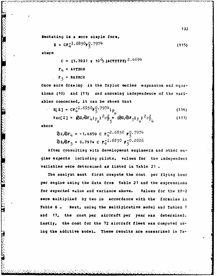
132
Restating in a more simple form,
14.68 500 .797 4
where
C = (1.7031 x 10) (ACTTyPE)2 .4 6 94
F4 = AVTBOH
F5 = BAXNCH
Once more drawing in the Taylor series expansion and equa-
tions (10) and (11) and assuming independence of the vari-
ables concerned, it can be shown that
z] = CF- 1'6950FO' 79 74 1P (116)
VarZ = ZZ/Z)F4ip )2a + (BZ/F5 p )25 (117)54
where
= -1.6850 C F-2.6850 FO7 974
ZZF 5 = 0.7974 C F741.6850 F50.2026
After consulting with development engineers and other ert-
gine experts including pilots, values for the independent
variables were determined as listed in Table 21 .
The analyst must first compute the cost per flying hour
per engine using the data from Table 21 and the expressions
for expected vdlue and variance above. Values for the XF-2
were multiplied by two in accordance with the formulae in
Table 6 * Next, using the multiplcative model and Tables 7
and 17, the cost per aircraft per year was determineJ.
Lastly, the cost for the 72 aircraft fleet was computed us-
ing the additive model. These results are summarized in Ta-

.- 6
133
TABLE 21
Spare Engine CER Variable Values
Name Var Acft L a H Mean VariancelI I
I VTBOH F4 XF-1 150 225 350 233 1111 1IF-2 200 275 300 267 278 1
AIMCHa F5 IF-I 1.95 2.05 2.00 .0008
XF-2 2.00 2.15 2.075 .0019
a - A range only was supplied for MAXMCH indicatinjall values within the range have equalprobability. Assumed a rectangular distributionwith mean and variance computed in accordancewith Table 10
ble 22 with detailed calculations for the XF-1 in Appendix
G.
TABLE 22
Engine Spares Yearly Cost Summary
Smillions FY83
IF-1 XF-2
- [X 4 1 7.967 13.052
I"SD[1 4 ] 0.229 0.171I"I
"%p
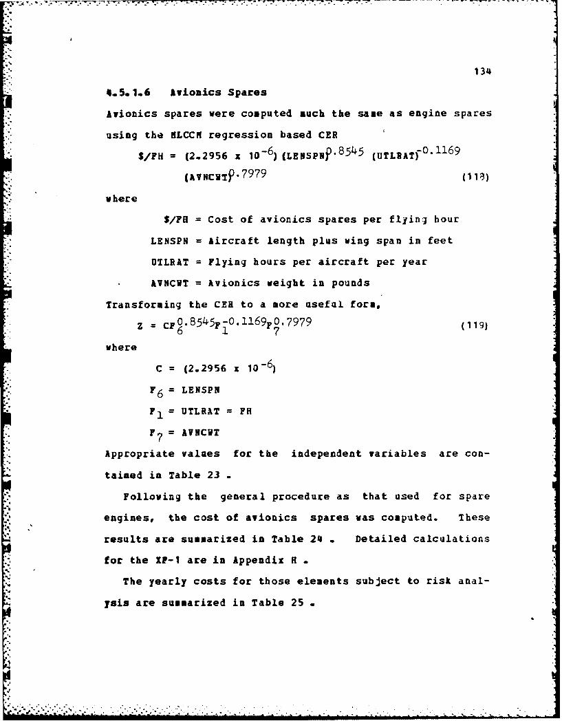
134
-. 5, 1.6 Avionics Spares
Avionics spares were computed much the same as engine spares
using the HLCCN regression based CER
S/PH (2.2956 x 10⁻⁶) (LENSPNP8 54 5 (UTLEAT) 0 1 1 6 9
(AVNCITP.7979 (11 3)
where
S/FH = Cost of avionics spares per flying hour
LENSPN = Aircraft length plus wing span in feet
UTLRAT = Flying hours per aircraft per year
AVNCVT = Avionics weight in pounds
Transforming the CER to a more useful form,0.55F0119O7979 19
Z C 6 1 7 (119)
where
C = (2.2956 x 10⁻⁶)
6 = LENSPN
F, = UTLRAT = FH
F = AVNCVT7Appropriate values for the independent variables are con-
tained in Table 23
Following the general procedure as that used for spare
engines, the cost of avionics spares was computed. These
results are summarized in Table 24 * Detailed calculations
for the XF-i are in Appendix H
The yearly costs for those elements subject to risk anal-
ysis are summarized in Table 25 .
• I . ' .. ' ' . . - . . . . . ... . . . .. ---.-,.,, ,,, " ,,... ,,,- - . ,, . ,, . , ...

- . r r y• ,r - . . . -s ' " - - . . . . -i "
. -i -
135
TABLE 23
Spare Avionics CER Variable Values
Naze Tar Acft L a H Mean Variance
3-LENSPNa F6 IF-I 80 85 82.5 2.08IF-2 100 105 102.5 2.0H
UTLPAT Fl Both 336 360 408 364 144
A VPCWTa y 7 XF-I 2500 3000 2750 20833 1XF-2 1500 1700 1600 3333
a - A range only was supplied for LENSPN and kVNCWT
indicating all values within the range haveequal probability. Assumed a rectangular and Imean and variance computed in accordancewith Table 10.
I I
I TABLE 24III Avionics Spares Yearly Cost Summary
I Smillions PY83II
IF-1 XF-2
I E-X5J 0..734 0.568
l SD[ X5 0.006 0.003
The equation for the expected value of the total yearly
cost, T, using the additive model is
3= C * E(z1 3 ..- * E-15] (120)
E4yl - "" + + " "5'

136
TABLE 25
Risk Analysis Yearly Cost Summary
$million FY83
Aircraft Element E( ] SD[X ]
IF-I X1 30.875 0.22912 29.248 0.20913 18.362 0.001X4 7.967 0-229S5 0.734 0.006
XF-2 X1 31.243 0.213
X2 35.189 0.14513 17.680 0.001X4 13.052 0.171115 0.568 0.003
where C is the most likely value of the sum of the cost
elements not subjected to risk analysis. For the XF-I,
ElY] = 35.310 + 87.186 = 122.496 (121)
and for the XF-2,
E[Y] = 35.384 + 97.732 = 133.116 (122)
Unfortunately, the variance is not so easily computel
since three of the elements, fuel (12), engine spares (X4 ) ,
and avionics spares (X5), are mot independent due to the
common factor, flying hours (Fl) , used in their respective
CER's. To compound the problem, the analyst's efforts to
secure subjective estimates of the covaridnces from the var-
-t ...- .° . .. " ..-" . ', . ' . j . : - . " - . . . • .

137
ious experts proved fruitless. Thus, the only recourse was
to determine the correlation between fuel cost and replen-
ishment spares for past and current related systems. This
was done in Table 26.
'i TABLE 26
jFuel/Spares Correlation
SI Smillions FY82
I Aircraft Fuel Sparesa
F-4E 13.450 1.798
I F-15 11.530 6.067
F-16 6.631 3.637
-1IF-111A 9.736 8.002
I r = correlation coefficient = -.23
a - Spares includes all spares. No separate breakdownfor avionics spares and engine spares is availablefror the source used.
9 Source: AFR 173-13II
Statistically, it is known that
Cov[X i,lj] = r SD[Xi] SD[Xj] (123)
where
Cov[i,Xj]= Covariance of Ii and Ij
r = Correlation coefficient

138
SD[Xi] = Standard deviation of Xi
Therefore, using the additive model in the dependent case,
Var[Y] = 1.2528EEll (124)
for the XF-1• and
Var[Y] 8.3889EE10 (125)
for the XF-2. The variances used in computing Var[T] are
listed in Appendix I . Next, the discounted expected cost
and variance over the operational life of the system *u-t be
computed.
4.5.2 Total Discounted Cost oRlutation
Before proceeding with the computation of total discounted
cost, some adjustment must be made to the year one and year
six costs to reflect the phase in and phase out of the sys-
tem. The best approach is to compute separate costs for
these two periods. It is assumed that production will be
evenly spaced throughout the year 1995 and that, likewise,
the retirement of the system will be evenly spread through-
out the year 2000 and that costs are proportional to the
number of active systems. Thus, there will be an average of
36 systems in operation during these two years. The analy-
sis was reaccomplished with 36 rather than 72 aircraft with
the results summarized in Table 27 . Taciances used in com-
puting Var[Y] are listed in Appendix I
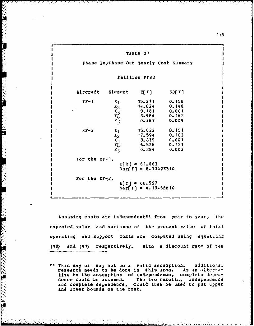
139
TABLE 27
Phase In/Phase Out Yearly Cost Summary
Smillion FY83
Aircraft Element E[X] SD[X ]
XF-1 X1 15.271 0.158X2 14.624 0.148
j1X3 9.181 0.001X4 3.984 0.162
X5 0.367 0.004
XF-2 X1 15.622 0.151X2 17.594 0.103
13 .8.839 0.001X 6.526 0.121 1A5 0.284 0.002
For the XF-1,ElY] = 61.083Var[Y] = 6.1342EE10
For the IF-2,E[T] = 66.557Var[Y] = 4.1945EE10
Assuming costs are independent 2 t from year to year, the
expected value and variance of the present value of total
operating and support costs are computed using equaticns
(40) and (41) respectively. uith a discount rate of ten
21 This nay or may not be a valid assumption. Additionalresearch needs to be done in this area. As an alterna-tive to the assumption of independence, complete depen-dence could be assumed. The two results, independenceand complete dependence, could then be used to put upperand lower bounds on the cost.
.° .. j.t i ... t 1...- -.-. - - - -

140
percent, application of these equations leads to the results
shown in Table 28 * It is important to note that the analy-
sis is as of 1983 in 1983 dollars. Thus, the first year
discounted is actually year thirteen and the last year
eighteen.
TABLE 28
Discounted Total OSS Costs
$millions FY83
XF-1 XF-2
E[PV(TOS) ] 141.159 153.481
SD[PV(TOS)] 0.184 0.151
Note: Var[PV(TOS) ] 3.3991EE10 2.2821EE10
4.5.3 Presenting the knalysi
Next an analysis and presentation of results is prepared.
Although rather obvious from Table 28 a mean-variance was
prepared as shown in Figure 17 ° From this plot, the deci-
sion maker's choice is not clear. The XF-1 has the lower
expected value, but the higher variance. Therefore, further
study is in order.

141
4.0 xXF-1
VariafGe 3.0(xO I0
I XF-2
2.0
100 125 150 175 1Mean ($ Millions)
Figure 17: FoF mean-Variance Plot
The computation of tolerance intervals is the next step.
Using equation (101) and Table 11 which assume a normal pop-
ulation and infinite sample size, tolerance limits were com-
puted such that at least ninety-five percent of the popula-
tion was included with a point nine five (.95) probability
level. These results were, for the IF-I,
(140.800, 141. 520)
and for the XF-2,
(153.190, 153. 780)
The choice is now cleaL. The tolerance intervals do not ov-
erlap and are, in fact, quite far apart. The XF-1 does in-
• • - - , ." , -m °% . . . . . . - . . . . .. "-

' ..
142
deed cost less to operate and support. The reader must how-
ever bear two things in mind. First, although the variance
of both systems was quite large, it is the square root of
the variance that is used in computing the tolerance inter-
vals and it is rather small by comparison. The second point
is that this estimate is for O&S costs only. Development,
acquisition, and, perhaps, disposal costs must be considered
in the life cycle cost evaluation. Development and acquisi-
tion costs could swing the pendulum in favor of the XF-2.
'The reader is reminded that this analysis is valid only
under the assumptions used in its preparation. The first
and foremost assumption is the fixed FoF scenario. This as-
sumption eliminates environmental uncertainty. Other as-
sumptions include:
1. Use of the additive and multiFlicative models
2. Use of the beta, rectangular, and Poisson distribu-
tions
3. Use of the normal distribution in computing yearly
O&S and total discounted OSS cost
4. Appropriateness of the CEB's
5. Adequacy of the Taylor series approximation
6. Independent cost from year to year
At this point, the risk analysis could be concluled, but
the analyst still has some unanswered questions. These will
be answered in performing an indepth risk analysis on se-
r. lected cost elements.
. ..

143
4.6 2.1k __h ISj ANALYSIS
After performing the preliminary risk analysis on the cost
drivers, an indepth detailed analysis should be accomplished
where warranted. Such an analysis gives greater insight
into the problem at hand. In this section, transforms will
be used to examine the fuel and engine spares CER's and the
depot maintenance analogy. The reader is reminded that the
probability distributions used are for illustrative purposes
and only the XF-1 will be used. Analysis of the XF-2 would
be analogous to that of the XF-i.
4.6.1 Fuel
The fuel CER, equation (107), models the product of a con-
stant and two random variables calling for application of
the Mellin transform. Assuming that flying hours (Fl), fucl
cost (F2), and fuel consumption (F3) are all triangularly
distributed, the transform of the Mellin convolution of the
•fuel CERis
f[g(Z) ] = Cs- 1 M[f(F 1 ) ] MCf(F 2 ) ] M[ f(F(1 ](1)
In the case of the XF-I, the first factor on the right hand
side is one. The Rellin transform of the triangular distri-
bution is contained in Appendix D and for the varidble F ap-
pears as
M[f(? ) ] - C 1 (360 s+1- 3 3 6S+L/(s+1 )
- ((336) ( 3 6 0 S- 3 3 6 s+l)/s]
+ C2C (408 S+1-(4 08) 36 0 S)Is
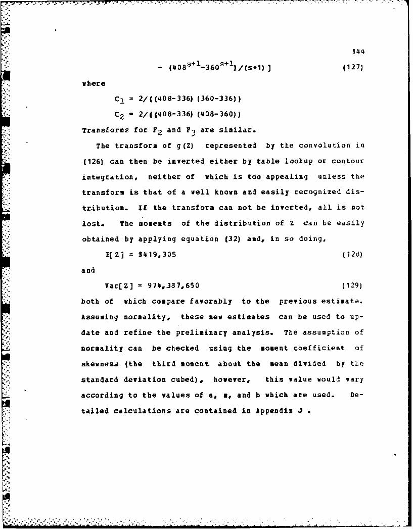
,, ., . ,. ,., . . ° . .. . . . . . . .. . .- " .' -'.• . . - - -" ".
144- ( 1 0 8 s+l- 3 6 0 +l)/(cs+) ] (127)
where
C 1 = 2/((408-336) (360-336))
C2 = 2/((408-336) (408-360))
Transforms for F2 and F3 are similar.
The transform of g(Z) represented by the convolution in
(126) can then be inverted either by table lookup or contour
integration, neither of which is too appealing unless the
transform is that of a well known and easily recognized dis-
tribution. If the transform can not be inverted, all is not
lost. The moments of the distribution of Z can be easily
obtained by applying equation (32) and, in so doing,
E[Z] = $419,305 (12d)
and
Var[Z] = 974,387,650 (129)
both of which compare favorably to the previous estimate.
Assuming normality, these new estimates can be used to up-
date and refine the preliminary analysis. The assumption of
normality can be checked using the moment coefficient of
skewness (the third moment about the mean divided by the
standard deviation cubed), however, this value would vary
according to the values of a, m, and b which are used. De-
tailed calculations are contained in Appendix J
'

145
4.6.2 j.jjDe $oaref[
The CER for spare engines, (88), is once again the product
of random variables. However, it is not a simple product as
in the case of fuel due to the exponents on the variables.
In spite of the complexity, it can be handled rather easily
by the Hellin transform. If
I = FE (130)
where F is a random variable raised to the E power, the Mel-
lin transform of the distribution of X is
R[g(Z) ] = NCf(F) ]Is=EsE+1 (131)
That is, the transform of F raised to the E power is the
transform of the distribution of F with s replacei by
(Es-E+1). For example, in the case of the spare engine CEia,
if one assumes that F5 is rectangularly distributed, then
the Nellin transform of the distribution of
V = F 9?4 (132)
is
HLg(W) = ((a~b) S-aS)/(sb) I s=.7974s-.7974+1
= (2 .05n - 1.95 n )/m (133)
where
n = .7974s+.2026
m = .07974s+.02026
Taking the moments in accordance with equation (32), it can
be easily shown that
[V] = 1.74 (13 )
Yar[V] = .0004 (135)

146
Assuming F is triangularly distributed and applyiuy the
above to that distribution, it can be shown that the MelliL
transform of g(Z) in (115) is
M[g(Z) ] = cs1 MIf(F) ]1s=-1.6850s+2.6850
P(f (P5) 's=.7974s+.2026 (136)
As in the previous case for fuel, the transform can be in-
verted and/or the moments can be obtained. Voing the lat-
ter,
E[Z) = 305 (137)
Var[Z) = 8459 (136)
which shows some change over the values previously obtained
in doing the preliminary risk analysis. Detailed calcula-
tions using transforms for this CER are in Appendix K
4.6.3 Depot Saintenance
Indepth risk analysis of depot maintenance provides an op-
portunity to demonstrate the use of the Laplace transform.
Assume that upon further discussion with the experts, the
analyst discovers that the values obtained for I and H in
the change applied to the taseline in equation (49) are re-
ally not absolute but are more like L6 and H5 discussed un-
der the gamma distribution and that there is some very small
possibility that cost say not exceed the base. ApproFriate-
ly, the analyst assumes that change (Z) is gamma distribute]
and applying equations (93)-(98) to the data in Table 19 for
the IF-i, the parameters of the gamma distribution are.1".;5 -: .. ... _ .... .. . ...

147
a= 37.9392 (139)
= 0.1627 (140)
Using the Laplace transform of the gamma distribution listed
in Table 10 and applying the shifting theorem [38:32] which
says that
LCf(X-a) U(X-a) ] = exp[-as] L[F(X) ] (141)
where the unit step function assures positiveness of the
transform, the Laplace transform of the model
X = 9 + Z (142)
is'
L[g(X)] = exp[-12.272s] (1+.1627sF379392 (143)
Applying equation (22), the moments can be extracted by tak-
ing appropriate derivatives of L[g(X) J with respect to s and
then evaluating at s=O . Such computation yields
E[] = S18.4428 million (144)
Var[X] = 1.0744 million (145)
Given the earlier assumptions in the section, these figures
compare favorably with those obtained in the preliminary
risk analysis. Detailed computations for the XF-1 are in
Appena1ix L
* , . . . . . . - . - * .-

148
The last step in the full, complete analysis is a sensitivi-
ty analysis. Traditionally, this is done by varying a cer-
tain parameter or factor and noting the resulting change ini
cost. If that parameter or factor is a random variable,
then a distribution accompanies that parameter or factor as
it changes. This calls for a repeat of steps one, two, and
* three in order to assess the full impact of the sensitivity.
4I.8 CONCLUDIG REMARKS
This chapter has demonstrated the feasibility of a risk
analysis under a typically realistic cost estimation scenar-
io using proven and accepted CER's and modeling techniques.
The four step approach offers a logical and reasonable way
to confront the risk inherent in any program. To quell the
objections to risk analysis discussed previously, more in-
foration is put before the decision maker, but it is infor-
mation that can contribute substantially to6 the decision.
In the case of the FoF, the decision maker would feel quite
comfortable in choosing the XF-i if the decision' were based
on discounted O&S cost. All decision makers have an inher-
ent appreciation for risk as they are faced with it each day
in every decision. Therefore, it is felt that decision mak-
*ers do not lack understanding in this area. As for those
who contend that the high numbers are too high, the width of

-- y
149
the tolerance interval is controlled to a large degree by
the standard deviation which is, of course, the square root
of the variance. in the problem presented, the variance was
quite large, but the standard deviation was quite small by
comparison. Therefore, the size of the numbers should not
be a deterrent, particularly when one does not know what the
numbers are in the first place. Lastly, risk analysis does
not unfavorably impact the credibility of the study but, to
the contrary, assures the decision maker that a thorough and#
complete analysis was done.
Theoretically, it is possible to do the whole risk analy-
sis using transforms. Practically speaking, this is easier
said than done. Starting with basic CER's and progressing
to yearly and discounted total OSS costs, the cathematicdl
expressions grow at each step to the point that they are
next to impossible to manipulate. The problem is compounded
when mixed additive and multiplcative models are used, forc-
ing the -,inversion and retransforsation of the expressions
involved. If one is only concerned with the moments of tLe
convolved distributions, the Mellin transform is far easier
to manipulate than the Laplace. This may force a prefcrence
to the multiplicative model. Lastly, the transforms can be
used quite easily and effectively in extracting the moments
necessary to apply the method of additive and multiplicative
moments introduced previously.

150
As a final remark, careful attention should be given to
the additive verses multiplicative model issue and its in-
*p .act on variance. Most CEP's were developed with a point
estimate in mind and from that standpoint, assuming indepen-
dence, it really does not matter which model is used. Hlow-
ever, when dealing with risk, the additive model can be used
to control and reduce the variance. This may be of some im-
port to those oho say the high numbers are too high. For
example, in the fuel CER, flying hours, fuel cost, and fuel
consumption rate were multiplied giving cost per aircraft
per year. In the case of the XF-1, this resulted in an ex-
pected value and variance of 406,224I and 604,766,259 respec-
tively. If the analyst believes that the fuel cost may vary
from one flying hour to the next depending on such things as
changes in flight profile and aircraft gross weight, then
the additive model is more appropriate. Using the additive
model, the expected value remains the same but the variance
is reduced to 1,168,903 ,a reduction of over 600 million.
Proper appplication of risk analysis should lead to a whole
new modeling. approach and set of CER's which are more re-
flective of reality and more accurate in terms of the actual
risk present.

.4,
Chapter V
SUNNARY, RECONNENDATIONS* AND FUTURE STUDIES
Life cycle cost (LCC) is one of the most controversial con-
cepts being discussed today within the Department of De-
fense. It is such an intuitively appealing concept that it
finds its way into the lexicon of virtually everyone in-
volved in acquisition decisions. Unfortunately, while the
concept itself is simple, implementation has proven to be
quite difficult. LCC cuts across traditional disciplines
and functional areas. It demands data from information sys-
tems designed for other purposes. It requires new methols
of analysis and revised business practices. Yet it holds
forth great potential in managing the nation's defense re-
sources.
This dissertation constitutes a critical examination of
life cycle costing and, in particular, operating and support
(O&S) costing. In that LCC activities are necessdrily a
part of a dynamic environment, this examination has been
from three perspectives: methodology, modeling, and applica-
tions.
- 151-0*4

152
Two 4spects of the dynamic environment give cLedence and
true meaning to life cycle costing. These are risk and un-
certainty. Without these, life cycle costing would be a
*eaninli;ess exercise. Yet it is these two aspects that are
the source of many problems associated with LCC. The LCC
estimate is the focal point of life cycle costing and, with
the inclusion of risk and uncertainty, it is a rdandoM vari-
able. The analysis leading to the estimate must address
these aspects through risk analysis in the case of risk and
se'nsitivity analysis in the case of uncertainty. Although
this requirement is well recognized, risk analysis, in par-
ticular, has received little attention. This paper ad-
dressed many of the fundamental issues related to risk and
uncertainty in LCC estimates.
5.1 METHODOLOGY
The key to the acceptance of life cycle costing as a deci-
sion and management tool is credibility. Steps must be tak-
en, both from an organizational and business practices point
of view, to ensure that credibility. LCC must be the con-
cern of everyone; in a word, it must be institutionalized.
As a step toward institutionalization, a mechalaism to en-
sure that the benefits of life cycle costing are actually
realized must be established. This may necessitate some ba-
sic reorganization, assignment of new responsibilities, and
changes in management practices.

153
Program uncertainty is the leading contributor to LCC
incredibility and is the leading reason why procurements go
astray. The key to program uncertainty is program stabili-
ty. Although instability can never be totally eliminated,
the government as a whole must take steps to increase sta-
bility. Congress should lengthen its planning horizon and
the Air Force must be~tter define its requirements. industry
cooperation is also essential and the benefits of increased
program stability will be reaped by all concerned.
if stability is the key to program uncertainty, then the
program manager is the key to LCC management implementatio.
With proper motivation, the program manager can be an effec-
tive force in the management, control, and inonitorir~g of
life cycle costs. But the program manager alone is not
enough!
Highly skilled and qualified analysts must be available
to assist. These analysts must be supplied with the tools
of their trade, data and modeling methods and techniqlies, in
order to perform their function. The data must be accurate,
complete, and readily available while modeling method3 aiid
techniques must be appropriate, consistent, and easily ap-
plied.
Most LCC estimates are presented as point or 'most like-
ly' estimates with no indication as to the inherent risk
contained in the estimate. This practice is dangerous an]

154
can be misleading. Further, the complete spectrum of infor-
mation regarding the estimate is not conveyed to decision
makers. In the chapter on modeling, risk analysis as it re-
lates to life cycle costing was fully explored.
5.2 NODELING
with the various cost factors and cost elements which con-
stitute the basis for the LCC estimate recognized as random
variables, risk analysis is a natural and necessary part of
the study. Risk analysis should be directed at the cost
drivers and falls into two broad categories: analytical and
Monte Carlo simulation. This study concentrited on the ana-
lytical category and presented three methods: additive and
multiplicative moments, sums and products of random vaia-
bles, and transforms. Major emphasis was placed an the last
two.
Seemingly overlooked in the literature, the sums and
products of random variables is a convenient-and easily im-
plemented method of performing a risk analysis. Although
sometimes requiring approximations, this method is applica-
ble in both the independent and dependent cases and requires
the least amount of information to be useful.
The method of transforms is more sophisticated mathemati-
cally than the sums and products of random variables, yet
produces more information on the random variables of con-
155
cern. This method, as presented, is only applicable in the
independent case. Two transforms, the Laplace for the addi-
tive model and the Nellin for the multiplicative model, were
addressed.
In applying any of these methods to O&S costs, the gener-
al modeling structure must be considered. In computing O&S
costs, factors are added and multiplied to arrive at cost
elements. This is done primarily through the techniques of
analogy and parametric costing. The cost elements are then
added to arrive at a yearly cost. Yearly costs are then
discounted and added to arrive at a total cost over the op-
erational life of the system.
When considering Monte Carlo simulation, the method of
additive and multiplicative moments, and transforms, the
choice of probability distributions for the random variables
concerned is quite important. Although there is a multitud4e
to chose from, the normal, log normal, triangular, beta,
rectangular, gamma, and Poisson are considered likeli candi-
dates.
After performing the risk analysis, its presentation to
decision makers is crucial. It must be clear, accurate,
precise, and easily understood. Various presentations in-
clude the mean-variance plot, tolerance intervals, cumula-
tive distribution curves, and floating bar graphs. But mod-
eling serves no real purpose in the absence of application.
I'

_77 7 7
'J.d
156
5.3 APPLICATION
By meals of a typical Air Force OSS cost scenario, it was
shown thdt a risk analysis is not only possible but reason-
able to perform using the methods and techniques discussel
in this paper.
In performing such an analysis, the four step appruach is
recommended. These steps are:
1. Determine most likely point estimate
2. Perform preliminary risk analysis on cost drivers
.3. Accomplish indepth risk analysis where warranted
4. Do sensitivity analysis
By following these steps, analysts and decision makers can
be assured that a complete, thorough analysis was done and
that a high level of reliance can be placed in the results.
5.4 IECOREMDATIOiS
Recommendations for improvement in the area of methodology
4 appear in the chapter by that name. They include changes in
business practices, reorganization of the acquisition pro-
cess with emphasis on the program manager, improved ddta
sources, and updated models.
In the area of modeling and risk analysis, increased uie
of the additive model would not only improve the model's ap-
proximation of reality but also portray a more accurate pic-
ture of the inherent risk. this recommendation is indepen-
dent of the modeling method used.
- . .:
" ,% ' "'%''.." '" / "" ,""- "" -"". "" -"."". ", ' " ." -... " .. ". " . .'

i
157
°lso, with the tools now at hand and the insight gained
through this research, risk analysis should be a required
part of every LCC and OS cost estimate. To do otherwise
would be a disservice to decision makers and a discredit to
life cycle costing.
5.5 FUTURE STUDIES
No study is ever complete in and of itself. As questions
are answered and problems solved, new questions and problems
take their place. Such is certainly the case with this re-
search.
Operating and support cost estimation in the dependent
case deserves more attention. As a first step, the nature
ard extent of the dependency must be explored and deter-
mined. The Visibility and Management of Operating and Sup-
port Cost (VAHOSC) program may provide the necessary data.
VAMOSC is, however, in its infancy and, at this point, may
lack the historical depth needed. When more is known about
the dependency, modeling methods can be devised and improved
to capture it. This may be particularly true for transforms
where joint distributions are necessary to model dependk ncy.
With reference to probability distributions, effort is
needed to determine the proper distributions for the various
cost elements which comprise O&S cost. At present, Desmat-
ics, Inc. is under Air Force contract for this study. When

1 58
the results are known, modeling methods can be devised to
take advantage of this newfound information. In the case of
. transforms, predetermined relationships could be developed
and used by analysts in the field thereby taking full advan-
tage of this powerful modeling tool.
Lastly, risk analysis and its impact must be studied from
the point of view of decision makers. In this research,
those who work for and supply information to decision makers
were interviewed. Once risk analysis becomes more accepted,
decision makers should be interviewed to determine the type
of presentation preferred and the extent to which risk anal-
ysis influences decisions.
The sky ahead is not without turbulance but with determi-
nation and perseverence, it will be navigated. The missioni
will continue as long as the Air Force requires new systems
for the defense of the nation.
NC
. . . . . . . .- - - - - -
C . . . . . . .
o. . .

Appendix A
UYTERVIEI ROSTER
)lame org~anlization
Raj Dev Devers OSD/PA&E
Lt Col Bob Ovens HQ USAF/ACM
Lt Col Rich Wiallace HQ USAF/ACMC
Lt'Col Gene Tattini HQ USAF/LEYE
Lt Col Don Crawford HQ AFSC/ACCF
Mr Frank Fong HQ AFSC/ACCE
Mr John Rosso HQ AFSC/ALPA
mr Vern Menker ISD/ACCL
Capt Arnie Douville &SD/ACCL
fr Mike Enright ISD/YZA
Mr Ron Vorhis ASD/TZPR
Mr Roger Steinlage HQ AFLC/ACME
Raj Paul Reid HQ AFLC/LC (VAMOSC)
Lt Col Larry Rice AFALD/XRS
ffr Tom Parry APALD/XRSA
Mr John Huff AF AL D/X RS &
Raj Les Takamura A?&FC/CWC
Dr Dick Taliaferro AFIT/LSY
Mir Boy Wood AIT/L ST
- 159 -

160
fir Virgil Rehg A FXT/LST
Capt Larry Esuelhainz APIT/LSY

Appendix B
GENERAL INTERVIEW QBESTIONS
The following general questions were asked of those. inter-
viewed:
1. what does your organization do with respect to life
cycle costing (OSS costing)?
a) What are the inputs to the organization? From
where do they come?
b) What are the outputs? To where do they go? For
what are they used?
c) From where and/or from whom do you get your direc-
tion and authority?
d) What, if any, decisions relating to LCC are made
by you or your organization?
2. As you see it,' what are the major strengths of life
cycle costing (OS costing)?
a) What are the major faults (problems) with life cy-
cle costing (OGS costing)?
b) What should be done to improve life cycle costing
(O&S costing)?
- 161-

* - - - -. * b - . 7 - -11.- 7 1 . .1 . . r w
162
c) Do you think life cycle costing has a credibility
problem?
3. Risk and uncertainty are facts of life. How sh.oul2
risk and uncertainty be addressed in life cycle cost-
ing (OSS costing)?
a) How can risk and uncertainty be reduced?
b) How should information relating to risk and uncer-
tainty be presented?
'-
°4

- - - - ... - -
.
Appendix C
ORGANIZATIONAL SPECIFIC INTERVIEW QUESTIONS
OSD 6 AF CAIG
1. What is the authority (regulations, etc.) for lite
cycle costiag?
2. What is required in preparing and presenting an esti-
mate?
3. For what do you use LCC estimates?
4. Is LCC really used in making decisions?
5. How much do LCC estimates influence decisions?
6. How worthwhile is risk analysis?
7. How should risk analysis results be presented?
8. What can be done about real world uncertainty?
9. How can real world uncertainty be addressed in terms
of risk analysis? "
10. What is the magnitude of real world uncertainty vers-
es cost estimating uncertainty?
11. Congress appropriates separate funds for acquisition
and support. Do you see this as a problem? If so,
what can be done about it?
- 163-
A-
- . I

- -. - -. . .. . , -. ~ . .- - .. .
A 164
12. Do decision makers understand random, stochastic pro-
cesses?
13. What really drives acquisition decisions?
USAF/ACMC
1. Hov are inputs to AFR 173-13 prepared?
2. What are the numbers (means, modes, etc.) in AFR
173-13?
3. Can risk and uncertainty information be incorporated
into AFR 173-13? If so, how should this Lnformation
be presented?
4. What is the CORE methodology?
AFSC/&CCE 6 APSC/ALPA
1. What is AFSC policy regarding LCC?
2. How do the product divisions differ with respect to
LCC issues?
ASDACCL
1. How do you see requirements for risk analysis affect-
ing program offices?
2. At the working level, is LCC policy and procedure
clear and concise?
ASj Program Offices
1. Do program office personnel understand risk analysis?
2. How would risk analysis affect your work load?
3. At the working level, is LCC policy and procedure
clear and concise?
AFL.AC..

- C.-* *' CC . 9- 'S * . ..mt . r *. *: . - ,. - . I , _ I
165
1. How is historic dita collected, treated, and dissemi-
nated?
2. What are the problems with the maintenance data col-
lection system?
3. How can risk information be included?
AFLC/LO VAMOSC
1. What is VAMOSC?
2. What does it offer?
3. How does it compare to other AFLC data collectioL
systems?
AFALD/XRS
1. At the working level, is LCC policy and procedurc
clear and concise?
2. Are regulations and instructions adequate?
AF!AEUcwc
1. How is data for AFR 173-13 collected?
2. Can risk analysis information be determined frox ex-
isting data?
AFIT
1. What do you teach in the areas of LCC and risk analy-
sis?
2. Are students aware of the stochastic nature of LCC?
- C -C -- - -C -C . . . . . .."-°

. .,2
Appendix D
THE TRIANGULAR DISTRIBUTION
Although rather easily derived from basic definitions, the
properties of the triangular distribution presented here are
rather lengthy due to the bounds placed on x and lack of
smoothness in the density function.
f~)=(2 (b- x) /(b-a) (b-u) m s s b
Let cl 21/((b-a) (a-a)) c 2 =2/ (b-a) (b-a))
E[x]Jfx dx c-~ x dx + c 2 f x(b-x) dx
=CJf (2.3-3a a2 0a 3)/6] *c 2 l( ( 3-3b 2 +2m3 )/61
Let E[x) =4.
Var~x] J 0 (x-4f(x) dx c fa Cr4)(-a) dx
+ lcJbM(x-4) (b-x) dx
-166-

167
It C?[ lb 3 2 3- (3b+3p) a 2 -3pb 2 + 6b) /6)
mbL[ f(x) ] f 00eSXfI d1 x = c I (x-a)e-sxdx c~J (b-x)e- Sdx
0 am
C ci (e - (-s.-1)@.Os(sa~l))/s2 +(ae s-aeca)S
c2 e~m~,~)e-sb 2 -sn -sbC21(e-mt-m-l+e (sb~l))/s *(be s-be )/s)
00 n
Nff(x)] x f x~fx) d x =ci.x s-r (x-a) dx0 a
+ C2f Isl~bx)dx
C 1C(ms+-as+ )(s+ 1) - (a. -a )/IsJ
c2 1 (bs+L-bms)/s - s+i ms+11sl

appendix 3
HAINTENANCE PERSONNEL CALCULATIONS
Type. Analogy
Data: Tables 13 14Il and 15
HP Base + Change = V + Z
E[MP] = V + E[ZJ = 1728 + 35 =1163
Var[IIP] = Var[Z] = 35
Using the additive model where the number of terms in the
sum is a random variable,
E[X] = E([1P] E[PAY] =(1763) (17513) =30,785,419
Var[XJ E[MP] Var[PAYJ E[PAY] 2 Varf NP)
=(1763) (23703700) + (17513) 2 (35)
=5..252L1EE10
-168-

Appendix P
FUEL CALCULATIONS
Type: Factor Based CER
Source: LSC Model
Data: Table 17
Z CFjF2 ?3
E[Z] = CFlF2 F3 1PU2 2 2 2
Var[Z] = ()Z/cFl1P) VCF1 + (BZ/'sF2JP CrF 2
+ (C)Z)BF 3j P) F
where
ZZ/F1= CF 2 F 3
Z)/Z 2= CF 1 F3
ZZ/aF 3 = CF 1?2
E( ZJ = (1) (36(4) (2.00) (558) =406,224
Var(Z) = (12145456) (144) + (4.1254&EE10) (.00CC)
+ (1529984) (756)
=604,766,259
Using the additive model for 72 aircraft,
E[XJ = 29,248,128
Var[XJ 4.3543EE10
-169-

Appendix G
ENGINE SPARES CLLCULATZONS
Type: Regression Based CER
Source: "LCCM
Data: Table 21
zCF= 1 .6850 FO 7974
where
C = (1.7031 x 10 ) (ACTTrPE)
E[Z] = CF1.68 50F,7974 1P
t7 Zrr) =F 45,,w ~22 (I ZOp )225ar[ Z
4Z/jF41 P P Fwhere
B2/ Z 4 = -1.6850 C F42 6 8 5 0 PO7974
Z,/F 5 = 0.7974 C F4 1 68 50 F 0.2026
E[Z] = C (233)-1.6850(2.0) 0"7974= 304
Var[Z] = (4.8202) (1111) + (14651) (.0008)
= 5367
Using the multiplicative model to compute cost per aircraft
per year,
E[X*] = (364) (5367) = 110,656
Var[X*J = (304)2 (144) + (364)2 (5367) + (144) (53u7)
= 7.2519-E08
- 170 -
* *4- " ~i~ 6
'e " ° i°
° .o. ° .. . ° .. •% % = .! " % " % • " % - , , " ," ." -' ," ' ' " , " •, -•
.- . ,.• .o
. ,.
m - - - m- . ." -.- , ,d - --- t. .. ' A , .- u .. = ,

171
Using the additive model to compute the cost for 72 air-
craft,
-~ - E[I] = 7,967,232
Var[XJ 5.2214EE10

- .. - . . . . . . q. . . . . . . .. i
',,
Appeadix H
AVIONICS SPARES CALCULATIONS
Type: Regression Based CER
Source: MLCCM
Data: Table 23
z = c 48545Fi°'169F0 "7 9 ?9
where
C = 2.2956EE-3
E[z] = C FV 8 545F10 .1 1 6
50 "7 9 7 ?P
2 2 2Z I 22Var[Z] = z)Z/)F 4ip ) 2224
'F+ Z/ZFF51P4 F 5
where
= .8545) C F O'I455F-O'II69FO 7 9 7 9
'.BZ/Zl 1 (-.1169) C F 8 54 5F-1'II 6 9FO 7 9 7 9
"Z/ZF 5 = (.7979) C F 8 54 5 F1 0 .1 1 6 9F50 . 2 0 2 1
E[Z] = 28.0
Var[Z] = (.0826) (2.08) + (.0001) (144)
+ (.0001) (20833)
2.2695
Using the multiplicative model, cost per aircraft per year,
* I* = F1 Z
Z[xf] = ELFl] EEZJ = 10,192
- 172-
t4'
=' %. , ,.,,,. ,, @ " . , . .. ,. . , - .. - _ . .,. . . , - .,. . - . .. ... . . ,I , , , . . :. ' - _ . , . , . . , , . , ' . . " . . ' , . . " . . .

173
Var X*] E[ Z]Var(F1 ] + E[ F,] 2 Var[ Z] Var[F 1 ] Var Z]
(28)2 (144) + (364)2 (2.2695)
*(144) (2.2695)
4 13g922
Using the additive model to compute the cost for 72 air-
craft,
EfI] = 733,834
Vart!] =29,802,384

Appendix I
COST BLENEIT VARIAICE SUIMADY
Risk Analysis Yearly Variance
Aircraft Element Var[l]
XF-i X1 5.2524EE10
X2 4. 3543EE10
X3 8. 4030EE05
X4 5.2214EE10
X5 2.9802EE07
XF-2 X1 4.5354EE10
X2 2.1035EE10
X I 2.5840EE05* - 3
X4 2.9350EE10
X5 8.7082EE06
45
Phase In/Phase Out Yearly Variance
-1754-

175
Aircraft Element VarI]
XI 2.4'963EE10
X2 2.1772EE10
X3 6..4600EE05
X4 2.6 I0lEEIO
X5 1-4901EE07
XF-2 X1 2.2677EE10
X2 1-05S18EE10
13 6.Li600EEO5
X4 1.L4675EE10
X5 4.3510EE06

4
. %
appendix J
RELLIV TRANSFORN EXAMPLE- FUEL CER
.N[g(Z) ] = cslN~f ~ ) ] M[f(F 2 1 ] Mff( 3) ]
Mif(x)] = C (ms+ -a S+j/(s.1) - (am S-a S+l)/s
+ c2 [(bs+1 -bmS)/s - (bS+l-aS+l)/(s l)] br
- c 1 V1 + c2 V2
vhere
CI = 2/ ((b-a) (m-a)), C2 = 2/((b-a) (b-m))
For F1 ,
cI = .0011574074 c2 = .0005787037
If s=2,
V1 = 101375.9999 V2 = 433152
If s=3,
V, = 35693568 V2 = 163012608
then,
Ef Fl] = 367.9999
E[F -] = 135648
V ar[Fl] = 3[? ] - Z[ F.1 = 224.0736
For F2 ,
c 1 = 266.6666 c 2 = 133.3333
If s=2,
- 176 -
• ,4.• . . . . ... . ...4' . . ' - , & ~ r
a" -- '

7 -77777 7w 77,
177
Vi .0024791667 V2 ' 010 16666
if s=3,
Vi .0049171875 V2 ' 020675
thenl,
Ef F2] 2.01672
EIF 2 1 4.067916665
Var[F 2] .0009722209
For P3
=i .0002020202 c 2 =.0001154401
if s=2,
V, 953999-9994 V2 =32214812.499
If s=3,
v, 505980000.1 V2 =1889891719
then,
Ef F3 ] =564.9999
*E[F 2 320387.5
Va r[ F3] = 1162.50117
Then*
E[Z] 419,305.3301
2E(z] 1.7679135EE11
4Var[Z) 974,387,650.9

Appeadji K
HELLIN TRANSFORN EXINPLE - SPARE EGINE CER
Z = C F~.6852 0.7974
where
C = 1.7031EE06
M[g(Z) ] = Cs-i11[f(F 4) ]s=-. 685s+2. 6850 l[ f(F5) ]s=.7974s+.2026
Assume F4 is triangularly distributed,C[(S+.1 S+i S- S+1
M[f(F4) ) = Cl[ (a -a S /(s 1) - (am -a )/s]
+ c 2[ (bs +-bm)/s - (b S+-a s+)/(s+1) ]
where
c1 = 2/((b-a) (m-a)) = .00013333
c 2 = 2/((b-a) (b-m)) = .00008
If s=2,
E[F 4] = c1 (2.096291903 - 1.715955431)
+ C2 (3.266001895- 2.610765295)
= .0001031305
If s=3,
EF4] = c1 (.0003248294 - .0002720343)
+ c2 (.0002552306 - .0001985804)
= .0000000116
Assume F is rectangularly distributed,5Iq[f(F5 )] - ((a+b) - a S/(sb)
- 178 -

179
where
a =1.95, b =.1
E[ F5 J 1.73793692
E[F 5 2 3.020824875
* - Then,
E[Z] 305.2539423
2E[Z ) 101639-808
Var[ZJ 8459.838678

11 7 DA133 023 LIFE CYCLE COSTING IN A DYNAMIC ENVIRONMENT(U) AIR 3/3FORCE INST OF TECH WRIGHT-PATTERSON AFB OH J A LONG1983 AFIT, INR-8-60
I UNCLASSIFIED FG51 NL

1 1.25 1"6
--
II.I II
MICROCOPY RESOLUTION TEST CHARTNATIONAL BUREAU OF STANDAROS-1963-A
!4
.................

Appendix L
LAPLACE TRANSFORM IUMPLE - DEPOT MAINTENANCE
X= + Z
Assume Z is gamma distributed
g (L6 + .95M +H6)/2.95 = 6.1727
-2 = ((H6 - L6)/3.25)2 = 2.8639
8=i i-f= .1627
If k=O,
= = 37.9392
Lfh(Z) ] = (1 + .1627sf 37 9 392
and
L[(X) = exp[-12.272s] (I1 + 1627s)-379392
E[X] 18.4428
Z[E X = 34l.2113
VirEXJ = 1.0744
-180-
-, -. / .' ",- ... :.,*s .':. ... :. " .. . . . . . ',. . . . , , ............. .. ........ .. ....... ..' .. . ...

BIBLIOGRAPHY
1. Aircraft Operating A& =)o Q20 Devj jme, guide.Washington, D.C.: Office of the Secretary of Defense,Cost Analysis Improvement Group, 15 April 1980.
2. AF Regulation 173-13. § j jjpd Z1. Factor.EWashington, D.C.: Department of the Air Force,Headquarters US Air Force, 1 February 1992.
3. AF Regulation 178-1. Economic Anlysis Aa4_ ZK2.jjEvaluation for lEoe~ Manjp~jg. Washington, D.C.:Department of the Air Force, Headquarters US Air Force,28 December 1973.
4. AF Regulation 400-31, Volume 1. iibiiU andMIanagement 2f UQ~aA.lg &1L Sipiorz Q£ji Prja !_oiand Prcdrs Washington, D.C.: Department of the?Air Force, Headquarters US Air Force, 30 September1982.
-.4q
5. AF Regulation 400-31, Volume 1. lisibilx I"Manaqgp~_&. g& Operating .nA Support C21. U.24ram ftt2ix-leu juvoort Cosj (jLS). Washington, D.C.:Department of the Air Force, Headguartwrs US Air Force,24 August 1982.
6. AF Regulation 800-11. LSj" Q2" Qs ljnnementProgram. Washington, D.C.: Departmet of the AirForce, Headquarters US Air Force, 22 February 1978.
7. Arrow. Kenneth J. Essays ig the Lhiau 2n Eoka&S Eal . Chicago: Markham PuBlishing company, 1971.
8. Babiarz, Captain Anthony S. and Captain Peter U.Giedras. "A Model to Predict Final Cost Groith in aWeapon System Development Program." Master's thesis,Air Force Institute of Technology, August 1975 (ADA016040).
S 9. Baker, William R. "Life Cycle Costing." PldjntEjaineecig 32 (Mlay 1978): 171-176.
- 181 -
.1
5. F eguaton 0031 VoueI. . .* .J~t
tSleSt_4e*~mr, u.*..o%** .o__sts ( C .7 -ahntn -..
Departmen o£ the......r......d...t.rs........o..e

182
10. Barry, Austin. Errors j Practical Measurement inScienge, Engineering, and Technol2.. New York, NewYork: John Viley £ Sons, Inc., 1978.
11. Berard. Andrew H. fe Cycle g Maagement,Methodology, and Case Studies. Ft. Belvoir, Virgi:ia:Defense Systems Management College, 1977 (AD-a052338).
12. Blanchard, Benjamin S. Design and Manage to Life gycleCost. Portland, Oregon: M/A Press, 1978.
13. Borch, Karl Henrik. The Economics of Uncertainty.
Princeton, New Jersey: Princeton University Press,1968.
14. Brown, Rex V. Research and the Credibji"1 2fEstimates. Homewood, Illinois: Richard D. Irwin, Inc.,1969.
15. Brown, Robert J. and Rudolph R. Yanuck. Life gxcleCosting: A Practical Guide for Eneray manaiges.Atlanta: The Fairmont Press, Inc., 1980.
16. Buckingham, Major General Charles E. "A Look atAcquisition Logistics." Air University Review. (May-June 1975): 35-40.
17. Canada, John R. Intermadiate Economic Analysis forManagement and Engineering. Englewood Cliffs, NewJersey: Prentice-Hall, Inc., 1971.
18. Canada, John R. and John A. White, Jr. Capita.Investment Decision inalysi "o management andEngiagerip. Englevood Cliffs, New Jersey: Prentice-Hall, Inc., 1980.
19. Churchman, C. Vest, Leonard Auerbach, and Simcha Sada,.Thinki Decisions Deductive 2uantitative nethosChicago, Illinois: Science Research Associates, Inc.,1975.
20. Cira, Captain Anthony T. and Captain Kenneth R.Jennings. "Life Cycle Costing: A Working LevelApproach," fMaster's thesis, Air Force Institute ofTechnology, June 1981 (AD-A103256).
21. Coon, Helen. "Note on William A] Donaldson's 'TheEstimation of the mean and Variance of a 'PERT'Activity Time'." O Relipn.s R..search 13 (Nay-June1965): 386-387.
183
22. C 9. Ovnershi Handl_2oL. Kirtland APB, New Mexico:Director of Analysis, Air Force Test and EvaluationCenter, May 1976.
23. Cost Uncertaiser e Analysis. EglinAPB, Florida: Coast Management and Technology Division,Directorate of Cost Analysis, Deputy for Comptroller,Armament Division, January 1982.
. 24. Cozzolino, John M. "A New Method for Risk Analysis."-. Sloan Management Review 20 (Spring 1979): 53-66.
25. Cramer, H. .athematij2 Methods of Statistics.Princeton, New Jersey: Princeton niversity Press,1946.
26- "Design to Cost and Life Cycle Cost," Amsterdam,Netherlands: AGARD Conference Proceedings No. 289, May1980 (AD A090098).
27. Dienemann, Paul F. s.imatinj Cost Uncartainxty qaiMonte Carlo Techniiues. Santa Monica, CaLifirniat TheRand Corporation, RI-4854-PR, January 1966 (AD-629082).
28. Doetsch, Gustav. Guide to the Applicati2n of LaulaceTransforms. London, England: D. VanNostranl CompanyLtd., 1961.
29. Donahue, James D. Products and Quots o1 ja4o~mVariable a__d T heir 2j2 jonS. Denver, Colorolo:The Martin Company, July 1974 (AD-603667).
30. Donaldson, William A. "The Estimation of the Mean andVariance of a 'PERT' Activity Time." OperationsResearch 13 (May-June 1965): 382-385.
31. Faber, Conrad V. Probabalistic Estimates with LimiteIData. St Louis, Missouri: US Army Aviation Research ,Development Command, Technical Memorandum TM 81-F-I,November 3980 (AD A093969).
1 32. Fallon, Richard. Suectiv sessment eoafUncevrtainty. Santa Honica, California: The RandCorporation, P-5581, 1976 (AD-026669).
33. Fisher, G. H. The Natue 2. acetait. SantaMonica, California: The Rand Corporation, 2-5133,November 1973 (AD-AO44831).
34. Fisher, Gene H. Coll Consideralions " fstemsknal .z- Santa Monica, California: The RandCorporation, R-490-ASD, December 1970.
4Z
4.
I:
184
35. Fleischer, Gerald A. isk and Uncertainty: Non:Deterministic Decisio M n in nqineering.Norcross, Georgia: American Institute of IndustrialEngineers, Inc., 1975.
36. Freund, Rudolf J. and Paul D. Minton. RegressionMethods A Tool For Data Analysis. New York, New York:Marcel Dekker, Inc., 1979.
37. Giffin, Walter C. Introduction to OerionsEngineering. Homewood, Illinois: Richard D. Irwin,Inc., 1971.
38. Giffin, Walter C. Transform ehnicues= ProbabilityModeling. New York: Academic Press, 1975.
39. Gnedenko, B. V. The Theory of Probability. New YoLk,New York: Chelsea Publishing Company, 1967.
40. Graves, Samuel B. "A Monte Carlo Risk Analysis of Life"- Cycle Cost Prediction," Master's thesis, Air Force
Institute of Technology, 1975 (AD-A021677).
41. Hahn, Gerald J. and Samual S. Shapiro. Statisticalm odels Enineeriq. New York: John Wiley & Sons,Inc., 1967.
42. Haight, Frank A. Handbook of the Poisson Distributior.New York, New York: John Wiley & Sons, Inc., 1967.
43. Haugen, Edward B. Probabalisti Aroaches .to Design.New York, New York: John Wiley 9 Sons, Inc., 1968.
44. Heinze, David Charles. Statistical decision AnaIlysioe anageen. . Columbus, Ohio: Grid, Inc., 1973.
45. Hertz, David 0. "Risk Analysis in Capital Investment."• 4_EavM-I Buss Review. 57 (September-October 1979):'5 169-181.
46. Hillier, Frederick S. j EvaIluation f RiskkInterrelated Investments. Amsterdam: North-HollandPublishing Company, 1969.
47. Hillier, Frederick S. and Gerald J. Lieberman.Ln troduction :2 q.atop Reseacch. San Francisco:Holden-Day, Inc., 1980.
48. Holts Charles A. Jr. and Robert V. Shore. BajyeianAnalysis J1 I 2oic Theory uIiu Sj~ eries Analysis.Amsterdam: North-Holland Publishing Company, 1980.
.. .. , "-a,-i, ". " , . . .-.. : " - -"" " " i . . ." " . . " . -- " . .- '

18'i
49. Hutton, 2. Bruce and William L. Wilkie. "Life CycleCost: A Ne Form of Consumer Information." Journal ofConsumer Rea b 6 (March 1980): 349-360.
50. Intervieve. Manual Revised Edition. Ann Arbor,Michigan: The University of Michigan, Survey ResearchCenter, Institute for Social Research, 1976.
51. Isaacson, Walter. "The Winds of Reform." Time 121(March 7, 1983): 12-30.
52. Jackson, P. S., R. V. Hockenbury, and M. L. Yeater."Uncertainty Analysis of System Reliability andAvailability Assessment." Nuclear EnQineerigj andDesiQn 68 (1981): 5-29.
53. Jewell, William S. Planni ngMA gontrol undg_ gisk.Berkley, California: Operations Research Center,University of California, Berkley, August 1976 (ADA037013).
54.. Joint AFSQ/AFLC Life Cycle Cost BanaQementInlementation Techniges Pamphlet. (Draftpublication.) Andrevs AFB, Maryland: AFSC/AFLC LCCSteering Group, July 1981.
55. Kahneman, Daniel and Amos Tversky. "Prospect Theory:An Analysis of Decision Under Risk." Econometrics 47(March 1979) : 263-291.
56. Kendall, Maurice G. and Alan Stuart. T .4y.kacedTheorj of Statistics. New York: Hafner PublishingCompany, 1967.
57. Kerran, John . and Lavern J. Menker. ife Cycle L ostProcurement Guide. Vright-Patterson AFB, Ohio: JointAFSC/AFLC Commanders' Working Group on Life Cycle Cost,ASD/ACL, July 1976.
58. Lamar, William E. Technica Evaluation Report onD o tO Cost wd U Le Slycle gost. AGARD AdvisoryReport No. 165, 16 July 1981 (AD A101447).
59. Laning, J. Halcombe, Jr. and Richard H. Battin. RandomProcesUe J1 Auoatic€ Control. New York, New York:McGraw-Hill Book Company, Inc., 1956.
60. Large, Joseph P. LW jA Initial Q jstUi_: Howk2o Estiae Lu Lancrease 1h Cost L 1"Viring Velpo-System. Santa Monica, California: The RandCorporation, -1467-PACE, July 1974 (AD-787395).
.. 4 .'..*. 4 .. v.....

186
61. Large, Joseph P., Harry G. Campbell, and David Cates.Pagametcic Equations o Estimating Aircraft Airframe" IM. Snata Monica, California: The Rand Corporation,R-1693-1-PAE, February 1976 (AD-A022086).
62. Lenox* Hamilton T. "Bisk Assessments," Master'sthesis, Air Force Institute of Technology, June 1973(AD-76787 1).
63. Life Cycle Cost Guide for Maio Weapon §11temS. NavalMaterial Command, November 1977 (AD A082273).
64. Lochry, Colonel Robert R. Fina Reor_ gf the USAFAcademy 11s Analysis Study L . Colorodo Sprinjs,Colorodo: United States Air Force Academy, 1 August1971 (AD-729223).
65. Logistics Support Q2" Iodel User's Lndbook Version_1.1 . right-Patterson APB, Ohio: Headquarters, AirForce Acquisition Logistics Division, January 1979.
66. Lukacs, Eugene. Charcteristic Functions. New York,New York: Hafner Publishing Company, 1960.
67. Marks, Ker Leth E., H. G. Hassey, and Brent D. Bradley.Life cle Cost gstimgtion Lo USAF Aircraft Sstms:1n Appraisal. of Cos,& Ijljmgjt jrtures and EstindtinqlMetbodologies. Santa Monica, California: The RandCorporation, VN-9925-AP, September 1977.
68. Martin, J. J. Baesil.n Decision Probles And mar ko- ains. Huntington, New York: Robert E. KriegerPublishing Company, 1975.
69. May, major Thomas E. Ortin I .Sprt g ltEstimating. Wright-Patterson APD, Ohio: Life CycleCost Management Division, Directorate of Cost Analysis,Comptroller, Aeronautical Systems Division, May 1992.
70. McClure, Lucille. kji Qjcle O Orlando,Florida: Martin Marietta Aerospace, October 1976 (ADA030554).
71. McNichols, Gerald R. "On the Treatment of Uncertaintyin Parametric Costing," PhD dissertation, The GeorgeVashington University, 1976.
72. Mendenhall, William and Richard L. Scheaffer.Aat atca.Il Statistics "t Applications. NorthScituate, Massachusetts: Duxbury Press, 1973.
4.A
* 187
73. Beakers Lavern J. Life cle Cost Anaysjs Guie4.18
Wright-Patterson AF!, Ohio: Joint AFSC/AFLC ComadndersOWorking Group on Life Cycle Cost, ASD/ACL, November1975.
,
N 74. Mitchell, Terence R. Uncertaiuj and Decision Makinq.Seattle, Washington: Department of Psycholojy,University of Washington, 1 September 1979 (AD-A074072).
75. _dl jjfe ycle Cost Model foK Advanced Aircraft3ystej._ Phase III, Volume V, Opeatinns and urtPhase j5jansion. Bethpage, New York: Grumman AerospaceCorporation, AFFDL-TR-78-40, Volume V, January 1980.
76. Moorev Peter G. Risk in B Decisions. Lonlon:Longman Group Ltd., 1972.
7% Norris, Peter A. "Combining Expert Judgements: ABayesian Approach." Management Science 23 (March1977): 679-693.
78. Morse, H. Stephen. _ C9j,. =Ajs of Risk AssessmentNethodolo ies. McLean, Virginia: System DevelopmentCorporation, 30 June 1980 (AD a089346).
79. Murphy, Edward L., Jr. Statistical Methols ofeasurn the Uncertainty of _Cst states. RedstoonArsenal, Alabama: Cost"AnalIsis Division, Comtrollerand Director of Programs* US Army Missile Command,February 1970 (AD-718862).
80. Naylor, Thomas H., Joseph L. Balintfy, Donald S.Burdick, and Kong Chu. gjmvuter Simultion 12ibniques.New York: John Wiley & Sons, Inc., 1966.
81. Neter, John and William Wasserman. Appied inJeaqStatistical Model. Homewood, Illinois: Richard D.Irvin# Inc., 1974.
82. O erating Support C evelopen Gude f ojjrajf System. Washington, D.C.: Cost AnalysisImprovement Group, Bay 1974 (AD a001747).
83. Ostle, Bernard and Richard V. Rensing. Statisticl jaIese.Xgh. Ames, Iowa: The Iowa State University Press,1975.
84. Parratt, Lyman G. k W.4 al &Pe.u.A ..isjjepM. New York, New York: John Wiley & Sons,
Inc., 1961.

P-
188
85. Paynev Stanley L. The Art 2I AsitPrinceton, Nev Jersey: Princeton University Press,1951.
86. Perry C. and I. D. Greig. "Estimating the Mean andVariance of Subjective Distributions in PERT andDecision Analysis." Management Science 21 (August1975): 1477-1480.
87. Poindexter, Lt Colonel Eugene 0. "Cost for DecisionMaking: A Synopsis." Armed Forces Comptroller (January1976): 16-23.
88. Pratt, John W., Howard Raiffa, and Robert Schlaifer.Introduction to Statistical Decision Theory. New York:McGraw-Hill Book Company, 1965.
89. ProceedinQs anaceent o Risk and Uncetain ty i.the Acguisition of Majr rg rals. Colorodo Springs,Colorodo: 0S-Air Force Academy, February 1981.
90. Quade, E. S. Analysis for MilitaUl Decisios. SartaMonica, California: The Rand Corporation, R-337-PH,November 1964.
91. Recktenwalt, Thomas J. The Air Forc Visibility andManagement of Operatin.q and Suprort Costs A Practicalpgach to 0S Costinq. Arlington, Virginia: paper
presented to 17th Annual DOD Cost Analysis Symposium,12-15 September 1982.
92. Sampson, Allan R. and Robert L. Smith. Asssessiag RsksTh _roq the Determination of RaSe Event Probabilities.Pittsburg, Pennsylvania: University of Pittsburg,Department of Mathematics and Statistics, July 1980 (ADA092192).
93. Schaefer, Donald F., Frank J. Husic, and Michael F.Gutowski. Monte Carlo Simulation Approach to Cost-Uncertainty Analysis. McLean, Virginia: ResearchAnalysis Corporation, March 1969 (AD-850054).
94. Schumacherg Villiam J. Life Cycle Costin_ and theEffect 2fOwnership Costs. Ft Belvoir, Virginia:Defense Systems Manap ment School# November 1975 (ADA027288).
95. Seldon, M. Robert. Lifa Cle Gostin : I Better Methodof Government procurement. Boulder, Colorodo: WestviewPress, 1979.
", .... ," .. . .......... .... . " -. .--..-.- ..-.- -,,...- .. . . . . .. . .

189
96. Selvidge, Judith. 8ethodology fr the RetrospectiveEvaluation of Decision Analysis. McLean, Virginia:Decisions and Designs 9 Inc., September 1976 (ADA035856).
97. Springer# H. D. The Algebra of Random Variables. Neworke Nev York: John Wiley & Sons 1979.
98. Sullivan, William G. and V. Wayne Claycombe.Pundamentals of Forecasting. Reston, Virginia: RestonPublishing Company, Inc., 1977.
99. Summers, Robert. Cost Estimate Ms Predictors ofLct_l I eapon Costs: j Study of Majorg HardwareArticles. Santa Monica, California: The RandCorporation, RM-3061-PR, March 1965 (AD-612723).
100. Thompson, Gerald E. Sta i_.igs for Decisions AnElementar Introduction. Boston: Little, Brown andCompany, 1972.
101. Us _ kjp2 T ji.j_ Assessing Cost Estimates (TRACE)Tuideljes. Hopeell, Virginia: John i. Cockerhar FAssociates, Inc., 31 December 1976 (AD-A036327).
102. Users _ f o. the T.ieshare Computer ProgramjWjsentationg of the Cost Oriented Resource Estimatin2(CORE) Model. Wright-Patterson AFB, Ohio: Life CycleCost Management Division, Directorate of Cost Analysis,Comptroller, aeronautical Systems Division, 30September 1981.
103. Wilks, Samuel S. thematica Statistics. Nev York:
John Wiley & Sons, Inc., 1962..
104. ora, George H. lopligation of Risk Analysi in tl.eAcquisition 21 Mao eapon Systems. Clemson, SouthCarolina: Clemson University, I August 1980.
105. Worm, George H. Applied Risk Analysis with DependanceAong g2 _t Compone . Clemson, South Carolina:Clemson University, November 1981.

An
UP
-f