DP2012-09 Agricultural Supply Response and Smallholders Market Participation

‒ the Case of Cambodia*

Md. Shafiul AZAM Katsushi S. IMAI Raghav GAIHA

March 16, 2012

* The Discussion Papers are a series of research papers in their draft form, circulated to encourage discussion and comment. Citation and use of such a paper should take account of its provisional character. In some cases, a written consent of the author may be required.

0  

Agricultural Supply Response and Smallholders Market Participation – the Case of Cambodia

Md Shafiul Azam* 

Economics, School of Social Sciences, University of Manchester, UK,

Katsushi S. Imai 

Economics, School of Social Sciences, University of Manchester, UK and Research Institute for Economics & Business Administration (RIEB), Kobe University, Japan

&

Raghav Gaiha 

Faculty of Management Studies, University of Delhi, Delhi-110007, India

16th March 2012

Abstract

This paper explores the key causal factors behind agricultural supply response and farmers' market participation decisions in Cambodia. A stylized farm household model with market imperfections is considered and a two-step decision making process is outlined. Farmers decide, first, whether or not to participate in the market and then they decide how much to sell. The model is estimated using a Heckman type regression model. We compute the unconditional marginal effects for the full sample as well as for the samples for the small and large holders separately. Non-price factors such as risk, technology and rural infrastructure are important determinants of commercialization of agriculture in Cambodia. The marginal effects for the small and large holders differ substantially both in quantitative and qualitative terms. This suggests differential treatment in terms of intervention and incentives for small and large holders would be more effective to promote market access.

Keywords: Agriculture, Supply response, Farm household model, Market participation, Switching model, Cambodia

JEL classification: Q12, Q13, Q15, C24 *Corresponding Author: Md Shafiul Azam (Dr) Economics, School of Social Sciences, University of Manchester, AL Building, Oxford Road, Manchester M13 9PL,UK ; Phone: +44-(0)161-283-0899; Fax: +44-(0)161-275-4928; E-mail: Md.Azam@postgrad.manchester.ac.uk Acknowledgements

We are grateful to T. Elhaut, Director, Development Studies and Statistics, IFAD, Dr. Ganesh Thapa, Regional Economist, APR, and K. El-Harizi, CPM for Cambodia, APR, for their encouragement and guidance at different stages. The views expressed are, however, personal and any remaining deficiencies are our sole responsibility.

1

1. Introduction

A vast majority of rural smallholders in developing countries depend on traditional and

subsistence farming, the characteristic features of which are, among others, low productivity

and low marketed surplus. These smallholder subsistence farmers are most likely to be

among the poorest and the most vulnerable of all groups. They remain mostly outside the

mainstream exchange economy and unable to take advantage of the opportunities offered by

an exchange economy. On the other hand, subsistence farming is often considered to be the

only means of survival against adversaries caused by market failures of various kinds, uneven

access to resources and the specific socio-economic and agro-climatic context under which

they operate. Hence, it is important to identify and address underlying factors leading to

subsistence farming and perpetuation of poverty and vulnerability of rural poor, because the

integration of smallholder subsistence farmers into the market mechanism through increased

participation and commercialization of agriculture would facilitate higher living standards

and reduce vulnerability.

The structure of and access to markets is critical in shaping the behavioural responses of

agricultural households in designing their livelihood strategy (Taylor and Adelman,

2003;Brooks, Dyer and Taylor, 2008). As long as markets are perfect for all goods (including

labour), households remain indifferent between consuming own-produced and market-

purchased goods. By consuming all or part of its own output, which could be sold at a given

market price, the household implicitly purchases goods from itself. By demanding leisure or

allocating its time to household production activities, it implicitly buys time, valued at market

wage from itself. Under these circumstances, the household effectively behaves as a profit

maximizing unit.

However, rural households in developing countries are often systematically exposed to

market imperfections and constraints, referred to as “failures” (Thorbecke, 1993). In some

cases, markets do not even exist, for example, in remote areas. In other cases where the

market exists, high transaction costs must be incurred in accessing markets. In yet others,

there are constraints on the quantities that can be exchanged (de Janvry and Sadoulet, 2006).

Moreover, as rural households are often unable to sell surplus labour at the going wage rate

on a year-round basis, they often have to pay more for foodstuffs than they can earn from

selling the same commodities, and risk is an inescapable fact of life for them all. Market

failures can therefore be pervasive and, coupled with uneven distribution and access to

2

operational land and other productive assets, and risks, poor rural households may be forced

to devise countervailing strategies against these adversaries which are at best suboptimal.

These countervailing strategies are likely only to compensate for a small fraction of the

market failures under which households operate, in part because the effectiveness of these

strategies is itself limited by poverty, and they are generally implemented at very high costs

in foregone expected incomes. In this fashion, poverty changes the set of options available to

households, making poverty hard to escape (Duflo, 2003).

There have been important theoretical advances on household behaviour under market

failures since the beginning of the 1980s. These modelling frameworks have largely been

successful in explaining and identifying strategic variables and some of the binding

constraints such as transaction costs, risk and other factors affecting the marketing behaviour

of subsistence/semi-subsistence farmers in developing countries. More importantly, the

insights derived from these efforts could be used for effective policy design to reduce poverty

and vulnerability. However, as noted by de Janvry and Sadoulet (2006 p177), more often than

not many theoretical derivatives and predictions emanating from these models are “blindly

accepted as truths when they remain to be empirically verified, their order of magnitude in

explaining observed behaviour remained to be ascertained, and their usefulness in the design

of policies to be shown”.

In light of the above observations, this paper intends to contribute to the empirical literature

by investigating the supply response of farm households under market failures due to

transactions costs and heterogeneous endowments. We take Cambodia as a case, an

overwhelmingly rural society characterized mainly by subsistence farming. In doing so, we

have taken account of the interrelationships among market participation, production and sales

decisions. We further investigate whether there are any systematic differences in behavioural

responses between small and large holders in terms of market participation and sales

decisions. This has strategic importance as this might call for differential policy interventions

for these two sub-sets of farming community and it is also important to focus attention on

policies to increase market participation of the smallholders (Sadoulet and de Janvry, 1995).

3

1.1. Background and Context1

Cambodia, a small Southeast Asian country, is an overwhelmingly agrarian society, where

agriculture outsizes rest of the economy. The country has just come out of a three-decade

long civil war and political conflict during which most of its social and physical infrastructure

was either destroyed or badly damaged. However, it has successfully managed its transition

to a market economy from a Soviet–style command-and–control economy during the 1990s.

Since then in a relatively stable macroeconomic environment, Cambodia registered a decade

of very high and sustained economic growth. In fact, it is one of only 46 countries to achieve

7 per cent average annual growth for 14 years in a row. As a result, the poverty head count

fell from 47per cent of the population in 1994 to 35 per cent in 2004, and then to 30 per cent

in 2007. The poverty magnitude has also fallen, from about 4.3 million people in 2004, to

about 3.9 million in 2007. However, poverty methodology is conservative and the poverty

lines are very low2. The stellar growth that led to poverty reduction of just 1per cent a year

with increasing inequality means that growth has not been particularly inclusive (ADB, 2011).

Agriculture remains a crucial part of Cambodia’s economy and accounts for 29 per cent of

the GDP in 2007. It employs around 59 per cent of the labour force. Agriculture has been

growing at 4.4 per cent over the past decade, against 4.0 per cent in Vietnam and 3.9 per cent

in Lao PDR. Growth in this sector is driven by mainly rice and, to a lesser extent, livestock

and fisheries. Eighty per cent of farmers grow rice, 60 per cent of them for subsistence. Rice

covered 2.6 million hectare in 2007 (two thirds of arable land and 90 per cent of cultivated

land) and production grew from 3.4 to 6.7 million tons between 1997 and 2007. Yields

remain low, however, (at 2.6 tons/ha, against 3.5-4.0 tons/ha on average in the region).

Cassava is a promising crop, but only 3 per cent of cultivated land is used for it. Considering

the dominance of rice in the overall economy of Cambodia, a substantial productivity

increase of rice culture is imperative. In view of the performance of its immediate

neighbours, a doubling of production per hectare of cultivable land is conceivable. With rice

culture being mainly the domain of family-farms, improved sector-performance as a whole

depends on them.

1 These stylized facts are drawn from (ADB, 2011) 2 The average national poverty line for Cambodia in 2007 was KR 2,473 per capita per day, or $0.62 at the exchange rate of

KR4,000=$1. The regional poverty thresholds were KR3,092 per person per day for Phnom Penh ($0.77); KR2,704 for

other urban areas ($0.68); and KR2,367 in rural areas ($0.59)).

4

At the heart of the problem thus, lies the need for a transformation from a primarily

subsistence- oriented agriculture, characterized by low use of inputs and low returns to land,

to a more commercially-oriented, more intensive agriculture. Given that the agricultural

sector is dependent mainly on family-based rice production, converting ‘smallholder’

households into an ‘emerging’ class of commercial farmers is of strategic importance. The

scope for such a transformation remains large; yet the capacity to modernize and benefit from

the opportunities of an evolving market economy seem limited. There are major obstacles,

ranging from the poor physical infrastructure resulting in high transport costs and poor

market integration, to low levels of education, training in new techniques and imperfect or

virtually non-existent rural credit and insurance market (Acker, 1999). In addition, the

specific topography of Cambodia may put a number of natural obstacles in the way of a

sustained intensification. Overcoming these bottlenecks will be the main key for achieving

sustained rapid economic growth based on expansion of increasingly productive employment

opportunities. In other words, the sustained productivity growth and intensification of

agriculture may lay ultimately with the limits of the rural development outreach itself. Given

the above context, an in depth analysis of market participation behaviour and its determinants

may help understand better appropriate policy choices for enhanced productivity and market

integration of small holders.

2. Review of Literature

The literature on agricultural supply response is vast and varied. Rather than going for an

exhaustive review of this enormous literature, this study sets out to review a subset of the

literature which is concerned with market participation and commercialisation of agriculture

in subsistence/ semi-subsistence agrarian economies. Even this subset of literature varies

considerably in several dimensions as it evolves over time – differences span from

motivational contexts to methodology and econometric methods employed; and thus they are

not directly comparable. The review is structured in the following chronologically distinct

phases: i) pre-farm household model era during the 1960s and 70s; ii) farm household model

era of late 1970s and 1980s; and iii) recent studies focusing on market failures.

Initial attempts to construct models of peasant production taking into account the fact that

peasant households have a dual character as both production and consumption units traces

back to 1960s in the Indian subcontinent, particularly in India. The primary focus of these

early modelling efforts was to explain the apparent lack of correlation between marketed

5

surplus and production of food grains. This generated a fair amount of scepticism and debate

over the usefulness of price policy for increasing the marketed surplus of food grains

(Krishnan, 1965; Nowshirvani, 1967; Askari and Cummings, 1974 and 1976). Some of these

studies also attempted to show that, in the case of the marketed surplus from peasant farms,

inverse/perverse responses were not only theoretically credible but in practice quite probable.

Askari and Cummings’ (1976) contention that, given land reform, availability of fertilizers,

pesticides, and irrigation, farmers will in fact respond to economic incentives by producing

and marketing larger quantities has been questioned by many observers. The objection has

been that while farmers may be responsive to price changes, their planting and marketing

decisions are primarily governed by traditional behaviour and practices, thereby making price

responses only of secondary importance in explaining output variation. Similarly, Mathur and

Ezekiel (1961), and Enke (1963) are of the opinion that the marketed surplus of subsistence

farmers may have fixed or relatively fixed monetary obligations and hence, only dispose of as

much of their production as is necessary to obtain the desired money income. The subsistence

farmers are most likely to be in debt because of social obligations or an unforeseen drought,

and thus in order to meet commitments in such circumstances; they need to sell a portion of

their produce. The result is that an increase in the price of product will be followed by a

decrease in the quantity disposed of, since a smaller quantity marketed can meet their cash

requirements. Olson (1960) and Krishnan (1965) have also suggested an inverse relationship

between the marketed volume of subsistence crop and price. They argue that an increase in

price for a subsistence crop may increase the producer’s real income sufficiently so that the

income effect on his demand for consumption of the crop outweighs the price effects on

production and consumption, and hence the marketed surplus may vary inversely with market

price.

It is also generally argued that the size of family in a household has a significant effect on the

marketed surplus as evidenced by the findings of Sharma and Gupta (1970). Larger family

size disposes of lower marketed surplus than smaller one, since the larger the family size, the

higher will be the quantity consumed, and less will be available for disposal. In other words,

an increase in the marketed surplus is likely to be siphoned- off by an increase in the family

size. Many earlier studies have also indicated that there is a strong link between marketable

surplus and output. They further suggest that the marketable surplus for the rice increases

more than proportionally to the increase in output and that the elasticity of marketable surplus

6

with respect to output is very high relative to the partial and total price elasticities. Such

findings were reported by Bardhan (1970), and Haessel (1975) in their respective studies.

Haessel (1975) argues that the elasticity of marketed surplus with respect to output is

substantially greater than unity. From the policy standpoint this means that, as output

increases, farmers will retain a smaller proportion for consumption purposes and make a

larger proportion available for off-farm consumption.

The development of farm household models in the late 1970s and early 1980s marked a

significant advancement in the theoretical as well as conceptual understanding of the issues

that hitherto remained unexplained or at best controversial. Building on the standard

production economics and the early 20th

century analysis by Chayanov (1926) of peasant

agriculture in Russia, these farm household models developed by Barnum and Squire (1979)

have been used to understand and analyse multitude of policy issues relating to rural

economies of developing countries. Particularly, these models have largely been able to

explain sometimes paradoxical – and even perverse – microeconomic responses of peasants

to changes in relative prices (Strauss, 1986; Lopez, 1984; de Janvry, Fafchamps, and

Sadoulet 1991). Several other theoretical and empirical studies have used similar modelling

approaches to analyse farm household responses under imperfect labour (Lopez 1984;

Benjamin 1992; Jacoby 1993; Sadoulet, de Janvry, and Benjamin 1998), or food markets (de

Janvry, Fafchamps, and Sadoulet 1991; Goetz 1992; Skoufias 1994; Abdulai and Delgado

1999). The distinctive features of these models emanates from non-separability3 rather than

standard neo-classical seperabiltiy assumption. The conceptual derivatives and the

predictions of these farm household models are, however, extremely sensitive to the set of

assumptions on which they are based (Brooks, Dyer and Taylor, 2008). As household’s

decision- making is assumed to be “recursive” in the sense that consumption and labour

supply decisions depend on its production decisions but not the other way round: production

decisions are independent of the other decisions (Singh, Squire and Strauss, 1986a). This

means that as far as production is concerned, the household acts as a profit-maximizing unit

as it would have done in a standard neoclassical set up. The on-farm production effect of an

increase, for example, in the price of staple unambiguously results in increases in labour input

3 A household model is said to be non-separable when the household’s production decisions are affected by its consumer

characteristics (consumer preferences, demographic characteristics, etc.); whereas, in a separable model, households behave

as a pure profit maximizing units. The profits, in turn, affect consumption, but without feedback on production decisions.

7

(waged/ or family, or both) and total production4 (Barnum and Squire, 1979, Chapter 3;

Singh, Squire and Strauss, 1986b, p.154). However, as a consumer, household now faces

higher staple price but at the same time experiences higher income due to higher profits from

farm production leading to a positive income effect competing with a negative substitution

effect. The net effect becomes ambiguous depending on the slope of the household’s utility

function as well as the magnitude of the profit effect. Hence, as a result of the “recursive”

relationship between the household’s consumption and production decisions, the supply

response of marketed surplus, especially at the market level, may turn out to be negative

(Barnum & Squire, 1979; Singh, Squire and Strauss, 1986b). However, non-separability

makes theoretical and, in particular, empirical analyses more difficult. Therefore, most

empirical analyses assume separable farm household models or use reduced forms of a non-

separable farm household model.

In contrast to early farm household model-based works, recent studies emphasize transaction

costs and institutional factors in determining households’ decisions on market participation

(Goetz, 1992; Key, Sadoulet and de Janvry, 2000; Vakis, Sadoulet, and de Janvry, 2003;

Vance and Goeghegan, 2004; Carter and Yao, 2002; Carter and Olinto, 2003). Goetz (1992),

in his pioneering work, estimated a switching regression model of market participation and

amount traded to grain market in Senegal – separating the decision of whether or not to

participate in markets from the decision of how much to trade. He found that fixed

transactions costs significantly hindered, while better information stimulated, smallholder’s

market participation. He also decomposed the impact of a rise in the price of grains between

entries of new sellers and increase in the sale of producers already in the market. Elaborating

the works by Goetz (1992), Key, Sadoulet, and de Janvry (2000) develop a model of supply

response when transaction costs cause some producers to buy, others to sell, and others not to

participate in markets. They consider fixed transaction costs (FTC) and proportional

transaction costs (PTC). Fixed transaction costs are invariant to the quantity of the good

traded, whereas proportional transaction costs increase proportionally in quantity. Thus, PTC

corresponds to constant marginal transaction costs. They estimated the model using data

consisting of Mexican corn producers and the results indicate that both types of transactions

4 It is important to distinguish between the supply responses of agricultural output and the marketed surplus. The above

analysis, which rules out perverse supply response, only applies to the former.

8

costs – fixed and variable – play a significant role in explaining household behaviour, with

proportional transaction costs being more important in selling decisions.

Heltberg and Tarp (2002) use Goetz’s approach to estimate reduced form equations for

market participation and value of food crops (as a group), cash crops (as a group), and total

value of crops sales, using data from a 1996-97 Living Standard Measurement Survey

(LSMS). Factors significantly affecting market participation included farm size per

household worker, animal traction, mean maize yield, age of household head, climate risk.

Explaining variation in the value of sales for food crops or cash crops was much less

conclusive, and the authors recognize that aggregation of sales into food or cash crop groups

may mask underlying causal mechanisms related to individual crop decisions. Henning and

Henningsen (2007) estimated a non-separable behavioural household model by incorporating

non-proportional variable transactions costs as well as labour heterogeneity along with fixed

and variable proportional transaction costs. The authors used household data from Mid-West

Poland. They confirmed that both transactions costs, including the non-proportional ones as

well as labour heterogeneity, significantly influence household behaviour, although in most

cases price elasticities remain the same.

Only a handful of such studies are available despite theoretical advances and most of them

are carried out in the sub-Saharan African context. To the best of our knowledge, there is

hardly any such study undertaken in the Asian context. Cambodia with its remarkably

undiversified and largely subsistence agriculture, lends itself to a very interesting case in this

regard. An empirical investigation of agricultural supply response taking into account market

participation behaviour of households under transaction costs would be a notable contribution

to the literature.

3. Theoretical Considerations

3.1. Transaction costs

Transaction costs are the embodiment of barriers to market participation by resource-poor

smallholders and have been used as a definitional characteristic of smallholders. It is also

considered to be one of the factors liable for market failures in developing countries (de

Janvry, Fafchamps, and Sadoulet, 1991; Sadoulet and de Janvry, 1995). Farmers generally

face transaction costs relating to market and information search, screening, enforcement,

bargaining, transfer, or monitoring. These costs tend to be higher for farmers living in remote

9

areas with poor infrastructures of communication and transportation. The farmers lack

information about the prices of products at the local level, and at final consumer’s level,

about quality requirements, about places and best periods for selling their products, about

potential buyers, about production in other areas; but also about their rights and the

legislative frameworks. Information about market demand is difficult and costly to obtain for

smallholders. Information may be obtained through contacts with other members of the

community but the accuracy of information is not guaranteed since those actors might have

‘opportunistic behaviour’. Thus, the distance to the market together with poor infrastructure

and poor access to assets and information may be manifested in high exchange costs, which

could be an impediment to enable many transactions to take place.

Transaction costs can explain why some farmers participate in markets while others are

simply self-sufficient. Differences in transactions costs as well as differential access to assets

and services to mitigate these transactions costs are possible factors underlying

heterogeneous market participation among smallholders. Transactions costs are broadly

categorized into fixed and variable (or proportional) transaction costs (Key, Sadoulet and de

Janvry, 2000). Fixed transactions costs (FTCs) may include the costs of: (a) search for a

buyer with the best price, or search for a market; (b) negotiation and bargaining – these costs

may be important when there is imperfect information regarding prices; (c) screening,

enforcement, bribing, and supervision – farmers who sell their product on credit may have to

screen buyers to make sure they are reliable. Farmers may have to screen potential input

sellers when there is asymmetric information as to the quality and the price of the inputs.

FTCs are invariant to the volume of inputs and outputs traded and are often lumpy since, for

example, a farmer may incur the same search cost to sell either one ton or ten tons of a

product. Once the information about the market has been obtained and contacts made with

the buyer, a household can sell any amount without having to incur extra costs.

Variable transactions costs (VTCs), on the other hand, include costs of transferring the

product or inputs being traded, such as transportation costs and time spent to deliver the

products to (or inputs from the) market. VTCs thus include the per-unit costs of accessing

the markets, which raise the price effectively paid for inputs and lowers the price effectively

received for output, thereby creating a price band within which some households find it

unprofitable to sell output or buy inputs. In general, while information variables are expected

to determine FTCs, measures of distance and transport are expected to determine VTCs.

10

3.2. Modelling Market Participation and Amount Traded

Agricultural output marketing decisions can be modelled as a two-step decision making

process: first, households decide whether or not to participate in the market, and then, they

decide on how much to sell. As opposed to much of the earlier empirical works on

agricultural supply response and market participation, recent developments in farm household

modelling under transactions costs (e.g., Key et al., 2000) allow interpretation of results by

distinguishing between fixed transactions costs, which influence only whether to participate

in the market or not, and variable transactions costs, which can influence both the decisions –

market participation as well as the amount traded. In addition, this distinction is also

important from technical as well as policy points of view. Technically, it helps to improve the

estimation procedure while yielding valuable insights into the effectiveness of particular

policy interventions for reducing transactions costs.

The conceptual framework of this study thus rests on a stylized static farm household model

incorporating transaction costs in line with Key, Sadoulet and de Janvry (2000). In order to

focus more on transaction costs, following Key, Sadoulet and de Janvry (2000) the model

ignores some aspects of households’ decisions, such as risk (price) and credit constraints. In

addition, ‘market participation’ is treated as a choice variable in the model. Households are

assumed to maximize utility with respect to consumption ( ), production ( ), input use (

), sales ( ), and purchase ( ) of each good . Goods consumed include

self-produced agricultural goods, market commodities and leisure. Households produce

agricultural products ( ) using labour, other variable inputs and land ( ).

In absence of transactions costs, households’ problem is to maximize utility function (1)

subject to constraints (2) – (4):

(1)

(2)

(3)

(4)

11

where stands for the market price, is the endowment of good , represents

exogenous transfers and other incomes and and correspond to household and

production characteristics, respectively. The cash constraint (2) states that all purchases of the

household must be less than or equal to sales and other exogenous income (A) such as

pensions, and remittances. The resource balance equation (3) states that the consumed and

sold quantity cannot exceed the production, endowment and purchased quantity of each good

. In the case of inputs , the resource balance states that sales, input use, and consumption

cannot exceed endowment and purchased quantity of each input . Equation (4) corresponds

to the production function that relates all inputs and outputs.

Now consider that market exchange involves transaction costs: proportional transaction costs

( ) corresponds to the costs incurred for each unit of marketed output sold and fixed

transaction costs ( ) which by definition are independent of the amount being transacted.

Similarly, in the case of purchase, proportional ( ) and fixed transaction costs ( ) occur.

With transaction costs equation (2) is transformed in equation (5):

(5)

takes the value 1 for the sellers and 0 for the autarkic households for each good , while

takes the value 1 for buyers and 0 for autarkic households. The equation suggests that in

the cases when sales involve transaction costs, the price received by the farmer will be the

market price reduced by the amount of the proportional transaction costs , since the

farmer has to incur this amount for each unit of sold product as a proportional cost. In

addition, marketing of each product will cost a fixed amount for the household. The

fixed transaction costs include, for example, costs of search for buyers, costs of collecting

information about the prices and the monitoring costs of the fulfilment of the contractual

agreement. Inversely, when buying goods, the household has to pay an additional

proportional transaction cost besides the market price for each unit bought. The

household also incurs a fixed one-time cost . The first order conditions of the

maximization problem of the utility function will yield the reduced form output marketed

supply, conditional on market participation (Goetz, 1992, Key et al., 2000).

12

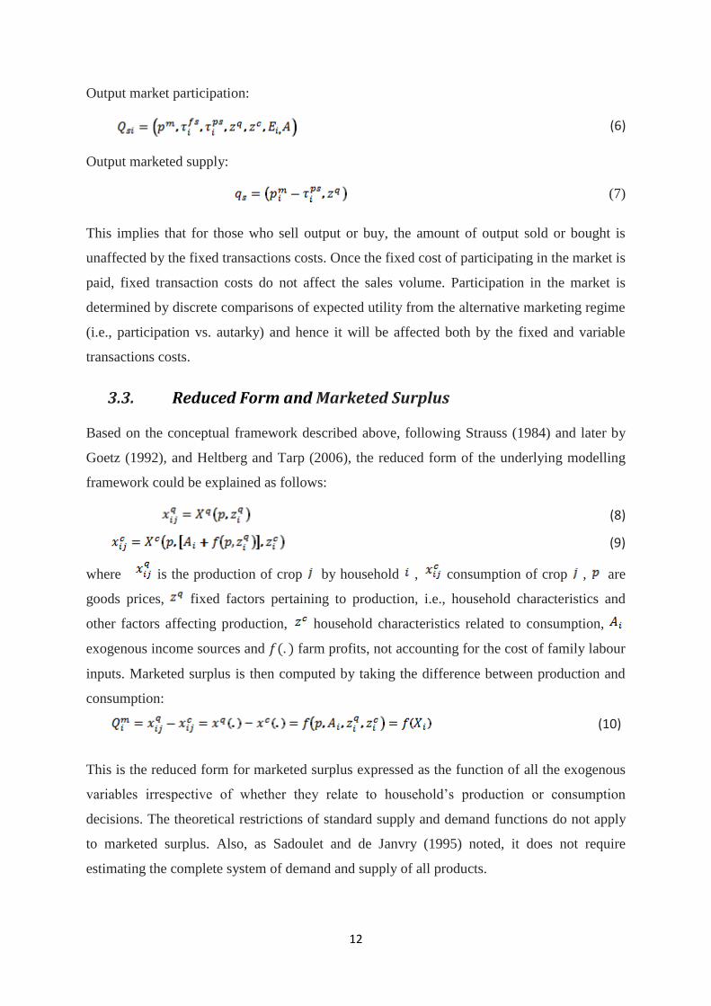
Output market participation:

(6)

Output marketed supply:

(7)

This implies that for those who sell output or buy, the amount of output sold or bought is

unaffected by the fixed transactions costs. Once the fixed cost of participating in the market is

paid, fixed transaction costs do not affect the sales volume. Participation in the market is

determined by discrete comparisons of expected utility from the alternative marketing regime

(i.e., participation vs. autarky) and hence it will be affected both by the fixed and variable

transactions costs.

3.3. Reduced Form and Marketed Surplus

Based on the conceptual framework described above, following Strauss (1984) and later by

Goetz (1992), and Heltberg and Tarp (2006), the reduced form of the underlying modelling

framework could be explained as follows:

(8)

(9)

where is the production of crop by household , consumption of crop , are

goods prices, fixed factors pertaining to production, i.e., household characteristics and

other factors affecting production, household characteristics related to consumption,

exogenous income sources and farm profits, not accounting for the cost of family labour

inputs. Marketed surplus is then computed by taking the difference between production and

consumption:

(10)

This is the reduced form for marketed surplus expressed as the function of all the exogenous

variables irrespective of whether they relate to household’s production or consumption

decisions. The theoretical restrictions of standard supply and demand functions do not apply

to marketed surplus. Also, as Sadoulet and de Janvry (1995) noted, it does not require

estimating the complete system of demand and supply of all products.

13

Using the results of equation (6 and 7), we further assume that both fixed and variable

transactions costs impact on market participation while supply decisions, conditional on

market participation, only depend on variable transactions costs. Technically, this implies that

we can use fixed transactions costs to identify market participation:

(11)

Finally, we postulate that variables that explain marketed quantities also explain the selection

of marketing regime, whereas fixed transaction costs help determine market participation, but

do not affect the amount traded conditional on being already in the market.

3.4. The Empirical Model and Estimation Strategy

While most empirical studies on output marketed supply or input demand have used

Heckman’s (1976) sample selection model or its variants of double hurdle and switching

regression models (e.g., Goetz, 1992; Winter-Nesson and Temu, 2005), some used the more

restrictive tobit model to analyse output marketed supply (e.g., Holloway et al., 2000). As

fixed transactions costs are expected to affect the decision to participate in a market, but not

the amount traded, the sample selection model has been considered more appropriate than the

restrictive tobit model. While tobit model assumes that “zero” values associated with non-

participation are outcomes of a rational choice (i.e., corner solutions), the sample selection

model explains non-participation using prohibitive transactions costs and other factors.

We estimate the econometric model using the framework of the standard Heckman sample

selection model, where the values of sales of agricultural outputs as well as the choice

between autarky and selling regime were determined jointly. Three sets of regressions are run

for: (i) total sales of all crops, (ii) sales value of marketed food crops, and (iii) sales value of

marketed cash crops, and each regression has both a selection and a value component. We

then split the sample into two parts: (a) a sample of small holders having operational land less

than or equal to one hectare, and (b) a sample of large holders having operational land greater

than one hectare and run each regression for them.

The econometric model is posited as follows:

(12)

(13)

(14)

14

where, is a vector of all the explanatory variables except fixed transaction costs ( ), and ,

, , and are parameters to be estimated. Subscript indexes households and crop

aggregation (total sales, sales of basic food crops, and sales of cash crops) is suppressed for

notational simplicity.

Sample selection model in marketed supply could be explained in two steps. In the first step,

selection into regimes i.e. selling, and autarky is modelled in separate probit type equation,

i.e., an equation for selling versus autarchy including fixed and proportional transaction costs

as well as all other explanatory variables. In the second step, the determinants of marketed

value conditional on market participation are analysed. Hence, both regressors and

parameters are allowed to vary across the two-steps and across regimes. In practice, however,

we estimate the model using maximum likelihood procedure which jointly estimates the

parameters of the selection and marketing equation. Standard errors are based on the Huber-

White estimator of variance and are considered robust against many types of misspecification

of the model. Covariance between the probability of participation and the quantity traded (the

’s) is captured by modelling the joint likelihood of market participation and marketed

values. However, interpretation of the coefficients is not straightforward as in the case of

OLS. Only those variables appear in the outcome equation (in this case, quantity equation)

but not in the selection equation, the coefficients of those could be interpreted as the marginal

effects of a unit change in the independent variables. If, on the other hand, the variables

appear in both the selection and outcome equations, the coefficients in the outcome equation

is affected by its presence in the selection equation as well. This is because both regressors as

well as the parameters are allowed to vary across the two-steps and across regimes (i.e.,

selling and autarky).

The other justification for employing Heckman sample selection model is to correct for

selectivity bias because selling households are non-random subsets of all sampled

households. Households might choose to participate in the market or not due to some

unobserved characteristics – risk aversion, farmer’s skill, or soil quality- and this is likely to

be the case where transactions cost barriers are important and a large segment of subsistence

farmers operate in autarky. Least squares without selectivity corrections would lead to invalid

estimates of the parameters for the full sample. Unconditional marginal effects (i.e., for the

full sample) cannot be derived from the least squares parameters and the possibility that

15

regressors might influence market regime and traded volume differently would completely

escape least squares analysis (Heltberg and Tarp, 2002).

3.5. Specification of the Model

Unlike some of the previous studies (Goetz, 1992; Key, Sadoulet and de Janvry, 2000), this

study uses aggregate value of sales as dependent variable. One of the major reasons for using

sales value rather than quantity marketed (i.e., in tons or kgs’) is to make most out of the data,

that is, to use all available information in the data, including those who produce and sell crops

other than rice or food crops. Moreover, due to substitution between crops, some exogenous

variables may increase individual crop sales at the expense of other crops. It is, however, now

well established that single crop supply is more elastic than the aggregate output supply.

Arguably, aggregate supply is what ultimately matters to policy makers (Binswanger, 1990).

Secondly, the choice of aggregating over multiple crops, on the other hand, makes it

impractical to work with quantities, because quantities produced or sold of different crops

cannot be aggregated directly. Values resolve this by using market prices as implicit weights

(Heltberg and Tarp, 2002). The greyer side of this kind of aggregation is that aggregation

conceals differences in the underlying causal mechanisms related to individual crop

decisions. Farmers may view differently in their portfolio of crop production, in which case

single crop estimation is necessary to provide the full picture. However, agriculture in

Cambodia is remarkably undiversified and characterized by mono-cropping (largely due to

its’ agro-climatic conditions), where paddy is being produced predominantly. Aggregation

over food crops is basically aggregation of paddy produced in dry and wet seasons.

Therefore, the aggregation bias discussed above is unlikely to pose serious problems in our

case.

Exogenous set of regressors include variables theoretically expected to affect quantities to be

sold as well as whether to participate in the market or not, that is, to select marketing regime.

Price of paddy is the most natural candidate to be included in the model. Paddy is the single

most important crop in relatively less diversified Cambodian agriculture. Over 90 per cent of

the cultivable land is devoted to paddy production. Hence, price of paddy is expected to be

the principal determinant of agricultural supply response in Cambodia.

Three variables are included in the model to capture the effect of household endowments:

land per worker, ownership of agricultural implements (plough, hand tractor, tractor or water

16

pump), and land title. Secured land ownership motivates farmers to invest in land

development and maintain soil quality. Theoretically, all these are expected to have positive

effects on marketed surplus and participation.

Ethnicity is included in the model to reflect the case that higher mutual trust and common

belief and understanding might affect the market participation through information sharing

thus reducing the fixed transaction costs. Theoretically, older and more experienced

household heads have greater contacts; allowing trading opportunities to be discovered at

lower costs; and this may also reflect increased trust gained through repeated exchange with

the same party. Among the other background characteristics of a household, a dummy for

households having any of its members employed in a paid job is included to take into account

non-farm earning opportunities.

Village level median rice yield is included in the model with a three- pronged objective of

capturing state of technology use, climatic condition, and past investment. A dummy for risky

region seeks to capture production risks posed by natural disasters - excessive rain, flood or

drought.

With a Heckman two-step approach, we first estimate a probit model of participation in the

relevant market as a function of both variables that are also likely to determine crop sales

volume, conditional on market participation as well as one or more variables that satisfy

exclusion restrictions (Wooldridge, 2006). Our exclusion restriction variables focus on the

factors affecting transactions costs. The exclusion restrictions we employ are similar to those

used by Heltberg and Tarp (2006) in their analysis of the determinants of market participation

in Mozambique.

Transaction costs are important determinants of market participation as well as the amount

traded, but they pose serious empirical challenges relating to measurement. First, when

transactions costs are too high to prevent exchanges to take place, then, by definition these

costs cannot be observed because no transaction has taken place. Second, even when a

transaction takes place, transaction costs cannot be easily recorded in a survey (Key, Sadoulet

and de Janvry, 2000). Transaction costs are thus unlikely to be observable in standard

household surveys. CSES-2004, 2007 data that we employ in our analysis is no exception in

this case. Hence, building on the past empirical works elsewhere (particularly Heltberg and

Tarp, 2002), this paper resorts to the observable exogenous variables that are theoretically

17

expected to capture or explain these transaction costs. Variables such as distance to market

outlets, ownership of transport equipments, and information/communication assets are

examples of exogenous determinants of transaction costs.

More specifically, variables used to capture transactions costs are: distance to nearest market,

distance to the nearest bus-stop, distance to the provincial capital, ownership of transport

equipments (cart, bi-cycle or motor-cycle), ownership of information/communication assets

(radio, television or telephone), village population density, and education of the head of the

households. By increasing travel time and transport cost, distance to market outlets (or bus-

stop, provincial capital) is expected to have a negative effect not only on market participation

but also on the amount traded. It is thus related to VTCs. The other VTCs – for example,

ownership of transport equipments- are expected to have positive influence on market

participation as well as quantity sold. Access to communication/information networks

essentially mitigates the fixed transactions costs and is thus likely to facilitate market

participation only. Other information variables included to capture fixed transactions costs

are education of head of household,5 and (log) of village population density. A better

educated head of household is assumed to be capable of higher level of information

processing and well- networked within the community. Similarly, in a densely populated

close-nit society information flow is assumed to be faster and better than in a sparsely

populated community. Both of these variables are expected to affect market participation

positively.

While ownership of transport equipments is also supposed to enhance market participation,

whether this is through its role in accessing information (FTCs) or in facilitating

transportation to market outlets (VTCs) is a question of empirical validation. This variable

might have dual roles: first, gathering market information by going physically to the nearest

market place; second, transporting farm outputs to the market. The empirical approach

proceeds by estimating and comparing the significance of two different versions of the

Heckman model, one with the variable used only in the selection (first stage) relating to

participation and another with the variable used in both participation and sales equations. The

preferred model would suggest the dominant attribute of transport equipment ownership –

information or transport attributes or both.

5 Alternatively, education could be included as an endowment variable as well.

18

Finally, the issue of endogeneity needs to be addressed. One might suspect potential

endogeneity of some of the variables used in the analysis; specifically ‘price of paddy’ and

‘land per worker’. The data on ‘price of paddy’ in our sample show considerable variation

both across villages and through the harvest season. As price varies depending on the place

and time of sale, it is potentially endogenous. Moreover, it is observed only for those farmers

who actually sold paddy during the period of the survey. Therefore, village level median

paddy price is derived and used in the analysis.

Cambodian land market is largely inactive and passing through a transitional phase from a

state-owned one to a market- based one. Land is largely state allocated and market turnover

of land is very low. In our data, land turnover is in fact less than 7 percent, which is

negligible from an analytical point of view. Hence, the variable ‘land per worker’ (defined as

total arable land holding divided by the number of economically active members of the

household) in our case is highly unlikely to be endogenous. In fact, the absence of an active

land market is the rationale given for the treatment of landownership as an exogenous

regressor in almost all the empirical works involving household behaviour in similar settings

in Africa and South Asia (Khandker, 2005).

4. Data, Variables and Descriptive Statistics

Data used for this study come from Cambodian Socio-economic Survey -2004 (CSES) and

CSES - 2007. Details about the data sets and variables used in the analysis are given below:

4.1. CSES - 2004

The CSES – 2004 is a standard LSMS type survey and is the first multi-objective household

survey undertaken in Cambodia. Data were collected over a 15 month period from November

2003 through January 2005. A total of 14842 households were interviewed in 900 villages

during a 15 month period The 2004 CSES is also the first household survey that covers the

entire country.

The 2004 CSES collected data on household consumption using two different data collection

methodologies, i.e., recall questions similar to those used in previous surveys and a calendar

month diary in which all household economic transactions were recorded. Consequently, the

CSES-2004 survey teams spent more than one month in each surveyed villages. In addition to

data on household consumption and a wide range of social indicators, the CSES collected

data on the daily time use of all household members, data on sources of household income,

19

village data on land use and access to community and social services (for examples, roads,

electricity, water, markets, school and health facilities), and data on up to three prices from

local markets for 93 food and non-food items.

2004 CSES sample was drawn from 45 strata (24 provinces, urban and rural) in three steps

using the 1998 population census as the sampling frame. First, 900 villages were selected

from the various strata using systematic random sampling. Second, one census enumeration

area was chosen randomly from each sample enumeration area, yielding a total sample of

15000 households (of which 14984 were actually interviewed). One thousand households

were interviewed each month of the survey in a randomly selected (and therefore nationally

representative) sample of 60 villages. The 2004 CSES is not self-weighting. Two sets of

adjusted sample design weight are provided, one for use with the calendar year 2004 sample

of 12000 households (of which 11993 households were actually interviewed) and the other

for use with the full sample of 15000 households (of which 14984 households were actually

interviewed). Estimates presented in this paper are based on the calendar year 2004 sample of

11993 households actually interviewed and are weighted to be representative of the

Cambodian population. Calendar year 2004 data are used to avoid introducing seasonal

biases. Table 1 provides all the variables used in the estimation of the model.

Table 1 Variables used in the Model

Variables Label Dependent

Log sales value food crops Natural log of Marketed Surplus of basic Food Crops Log sales value cash crops Natural log of Marketed Surplus of Cash Crops Log sales value-all crops Natural log of Marketed Surplus of all Crops Explanatory – Log price of paddy Natural log of village level median Price of Paddy Explanatory – households’ background Characteristics Log age of hhh Log age of head of the household in years Dependency ratio Dependency ratio Dummy for ethnicity Dummy for the Ethnicity (Khmer=1, 0 otherwise) Dummy for paid job Dummy for whether any member of the household has a

paid job or not Explanatory – households’ Endowments Log land per worker Natural log of farm size per worker Dummy for land title Dummy for whether household has land title or not Dummy for ownership of ag. Equip Dummy for ownership of agricultural Implement (Plough,

hand tractor, tractor or water pump) Explanatory – Geographical and technological Characteristics

Log rice yield (village level) Natural log of median village level rice yield Dummy for risky region Dummy for risky region – region reported most crop

damage due to excessive rain, flood or draught last year Explanatory – Variable Transaction Costs Log distance to market Natural log distance to nearest market Dummy for ownership of transport equipments Dummy for ownership of transport equipment – cart, van

etc. Log distance to bus stop Natural log distance to bus stop

20

Log distance to provincial capital Natural log distance to provincial capital Explanatory – Fixed Transaction Costs Log village population density Natural log of village population density per square

kilometre Dummy for ownership of radio, tv, or telephone Dummy for ownership of information equipment – radio,

TV, or Telephone Education of hhh Educational level of the head of the household

Table 2 Descriptive Statistics (CSES – 2004)

Variables Mean Standard deviation Minimum Maximum

Log sales value-all crops 12.746 1.52 5.7 18 Log sales value food crops 12.779 1.44 5.7 18 Log sales value cash crops 12.379 1.59 7.1 18 Log price of paddy 6.088 0.24 3.9 7 Log land per worker -1.240 1.22 -10.3 4 Log age of hhh 3.752 0.32 2.9 5 Dependency ratio 0.817 0.70 0.0 6 Dummy for land title 0.554 0.50 0.0 1 Dummy for paid job 0.283 0.45 0.0 1 Dummy for risky region 0.064 0.24 0.0 1 Log rice yield (village level) 7.340 0.56 6.2 12 Dummy for ownership of ag. Equip. 0.491 0.50 0.0 1 Dummy for ethnicity 0.961 0.19 0.0 1 Dummy for ownership of transport equipments 0.728 0.44 0.0 1 Log distance to market 1.528 1.20 -2.3 5 Log distance to bus stop 2.065 1.58 -2.3 6 Log distance to provincial capital 3.451 0.84 0.0 6 Dummy for ownership of radio, tv, or telephone 0.619 0.49 0.0 1 Log village population density 7.015 0.73 4.6 10 Education of hhh 5.729 10.54 0.0 19

Number of Observations 11862

4.2. CSES – 2007

The Cambodian Socio-economic Survey -2007 is similarly a standard LSMS type survey

comprising data from 3598 households from 360 villages. These villages are in fact

subsample of the CSES-2004, but the households are not necessarily the same as in 2004.

There are various modules containing detailed households and village characteristics

including households’ socio-economic characteristics, economic activities – crop production,

consumption of food and non-food items, health and education status, access to social and

community services. Table 3 gives descriptive statistics for all the variables used in the

estimation of the model for CSES-2007.

21

Table 3 Descriptive Statistics (CSES - 2007)

Variables Mean Standard deviation Minimum Maximum

Log sales value-all crops 13.46 1.60 -3.47 17.74 Log sales value food crops 13.54 1.57 8.51 17.77 Log sales value cash crops 13.08 1.58 -3.46 17.76 Log rice yield (village level) .93 .22 .39 1.34 Log price of paddy (village level) 4.38 2.93 0 7.17 Dummy for risky region .53 .50 0 1 Log land per worker -.92 1.19 6.50 3.91 Dummy for ethnicity .98 .16 0 1 Age of head of households in years 44.86 13.80 16 91 Dependency ratio .79 .68 0 5 Education of hhh 4.37 3.63 0 19 Dummy for land title .58 .49 0 1 Dummy for ownership of ag. Equip. .38 .49 0 1 Dummy for ownership of transport equipments .25 .43 0 1 Dummy for ownership of radio, tv, or telephone .74 .44 0 1 Log distance to market 1.58 1.20 -2.30 4.59 Log distance to bus stop 2.065 1.58 -2.3 6 Log distance to provincial capital 3.451 0.84 0.0 6 Dummy for paid job .41 .49 0 1 Log village population density 7.015 0.73 4.6 10

5. Results We estimated the model using two different sets of household survey data namely CSES –

2004 and CSES – 2007 for Cambodia as described in the previous section. CSES – 2004 is

the most comprehensive household data and more representative than the CSES – 2007 data

although they share same questionnaire and similar methodology in terms of sampling and

other attributes. Hence they are comparable and the results from the CSES – 2007 data should

provide some sense of validation of our initial estimates. In what follows, we first present the

results of our initial estimates based on CSES – 2004 data and then the results based on CSES

– 2007 in the next subsection.

5.1. Estimates Based on CSES - 2004

As noted earlier, the coefficients of the two stage selectivity models can not be interpreted as

marginal effects when the same set of exogenous variables appear in both the selection and

outcome equations. Accordingly, we have computed unconditional marginal effects

(computational procedure is given in Appendix 1) for all the models. The marginal effects6

for all households, large holders (farmers who have more than one hectare of operational

land) and small holders (farmers with one hectare or less operational land) across crop types

are presented in figure 1, 2, and 3 respectively along with the regression results (Table 4, 5,

and 6). For each model, there are two columns: first column reports the log of annual sales

6 For details about marginal effects of selectivity models please see Huang, Raunikar, and Mistra 199;

Hoffmann, and Kassouf 2005; Sigelman and Zeng 1999.

22

given market participation and the second column shows the results of market participation

probability model. However, our principal focus would be to disentangle distinctive (if any)

features of agricultural supply responses between small and large holders emanating from

their behavioural and other attributes and analyse welfare implications for

subsistence(mostly smallholders) farmers. Accordingly, we will touch upon some of the main

findings of the overall model in this section and then move on to the next section where we

compare the marginal effects as well as the regression results for the small and large holders.

Figure 1 Marginal Effects across Crop

23

Table 4 Regression Results (Heckman Sample Selection Model), Dependent Variable = log Sales value of

marketed Surplus Food Crops Cash Crops All Crops

Variables Quantity Select Quantity Select Quantity Select

Log median price of paddy (vill) 0.347** 0.784*** -0.369* 0.366*** 0.349*** 0.737***

(2.90) (10.74) (-2.09) (4.96) (3.38) (10.64)

Log land per worker 0.772*** 0.663*** 0.257*** 0.129*** 0.734*** 0.557***

(15.99) (33.28) (5.28) (7.08) (19.35) (30.21)

Log age of HH 0.420*** -0.0283 0.239 0.306*** 0.498*** 0.147*

(4.27) (-0.43) (1.45) (4.47) (5.72) (2.34)

Dependency ratio -0.00217*** 0.00345*** -0.000014 0.000181 -0.00209*** 0.00245***

(-4.59) (-12.48) (-0.02) (-0.67) (-5.43) (-9.56)

Dummy for land title -0.0699 -0.0122 -0.293*** 0.0776* -0.127** 0.0472

(-1.32) (-0.35) (-3.62) (2.17) (-2.73) (1.41)

Dummy for paid job 0.0825 -0.0573 0.0149 0.00889 0.0762 -0.0558

(1.15) (-1.23) (0.15) (0.19) (1.23) (-1.27)

Dummy for risky region -0.638*** -0.484*** -0.442** 0.345*** -0.426*** -0.111

(-5.01) (-6.99) (-2.99) (5.46) (-4.81) (-1.81)

Log median rice yield (vill) 1.075*** 0.787*** 0.331*** 0.0964** 0.932*** 0.644***

(15.87) (23.47) (4.80) (3.06) (17.66) (20.58)

Dummy for ownership of ag. Implements 0.417*** 0.220*** -0.139 0.244*** 0.301*** 0.264***

(6.75) (5.72) (-1.41) (6.15) (5.58) (7.33)

Dummy for ethnicity -0.171 0.0837 -0.503 0.202 -0.144 0.150

(-0.93) (0.76) (-1.91) (1.79) (-0.93) (1.48)

Dummy for ownership of transport

equipments

0.171* 0.0658 0.111 -0.00574 0.180** 0.0383

(2.56) (1.53) (1.13) (-0.13) (3.16) (0.95)

Log distance to market -0.0459 -0.0484** -0.108** 0.0663*** -0.0512* -0.00394

(-1.87) (-2.92) (-2.84) (3.90) (-2.39) (-0.25)

Log distance to bus stop 0.0613** 0.0565*** -0.0554 0.0925*** -0.0259 0.00425

(3.18) (4.55) (-1.81) (-7.52) (-1.64) (0.36)

Log distance to provincial capital -0.0236 -0.00821 -0.0772 0.0843*** -0.0255 0.0173

(-0.60) (-0.33) (-1.39) (3.43) (-0.78) (0.74)

Dummy for ownership of radio, TV, or

telephone

0.0677 0.0919* 0.103**

(1.83) (2.54) (2.89)

Log village population density 0.00501 0.179*** 0.0910**

(0.17) (6.22) (3.17)

Educational level of HH 0.00337* 0.00120 0.00216

(1.98) (0.73) (1.27)

Constant 1.259 -10.15 13.86 -6.644 2.470 -9.981

(1.10) (-15.84) (7.74) (-10.34) (2.54) (-16.48)

N 6978 6978

t statistics in parentheses * p < 0.05,

** p < 0.01,

*** p < 0.001

24

5.2. Summary of Results:

All Households

The price of paddy, the most important crop in Cambodian agriculture cultivated in

more than 80% of the arable land, has expected positive sign and significance in

almost all the equations. For all crops and food crops, price of paddy has significant

positive effect and for cash crops it has negative but significant effect. This is

theoretically consistent as higher paddy price induces households to produce more of

the product rather than producing crops that are relatively less profitable. The

marginal effect of price of paddy accordingly comes out to be highest in magnitude.

An interesting finding is that higher price of paddy not only results in higher marketed

surplus of rice, it also motivates households to diversify their portfolio of crop

production. As price increases so does profit and income of the farmers and better- off

farmers can now afford to produce more cash crops resulting in increased market

participation and commercialisation of agriculture.

Based on the CSES – 2004 data, except land title (which is very important for small

holders that we will discuss later), the coefficients for other capital endowment

variables, namely - land per worker, ownership of agricultural implements – are

positive and highly significant for both quantity and market participation equations,

indicating that relatively well-endowed farmers participate in the market and

commercialize. The marginal effects for these two variables are also among the

highest (3rd

and 4th

, respectively). This is even more important for the smallholders’

group (fig.2).So interventions that build households’ agricultural assets and intensify

cropping pattern (expansion of new arable land is constrained by cost of demining,

and redistribution is politically not feasible) could pay higher dividends in terms of

poverty reduction, through increased market participation and commercialisation of

agriculture by smallholders.

The dummy for risky region, as expected, has the largest (absolute) negative marginal

effect on food crop marketed surplus while the opposite is true for cash. This is an

interesting finding. Food crop is dominated overwhelmingly by paddy in Cambodia

which is susceptible to damage due to disasters such as excessive rain, flood, or

drought. Farmers in disaster prone region opt for safer but low return crops such as

mango/ or banana resulting in potential food insecurity/ persistent poverty and

vulnerability (or possibly a geographic poverty trap). This is particularly true in a

25

subsistence economy characterised by imperfect credit and insurance markets. Hence

living and farming in risky regions clearly does not help market integration and

commercialization of agriculture.

Marginal effect of village level median rice yield, a variable capturing combined

effect of geographic features, state of technology use and the effect of other inputs is

of considerable significance. Increased rice yield not only results in larger marketed

surplus of rice itself, it also helps generate larger marketed surplus of cash crops.

Improved rice/food productivity can drive commercialization of other crops as it

potentially could free up land and other resources tied up in subsistence farming. For

smallholders this has the highest marginal effect. This is true for both sets of estimates

based on CSES – 2004 and CSES – 2007.

Factors capturing variable transaction costs, except transport equipment ownership,

have in most cases (both in selection as well as sales/quantity equations) expected

signs and are significant. Thus variable transaction costs constitute one of the major

binding constraints to market participation and commercialisation of agriculture in

Cambodia which is an important finding with significant policy implications. This is

particularly important for smallholders. The coefficient of (log) distance to market for

this group is negative and highly significant in both participation and quantity

equations. So providing better access to markets is likely to induce smallholders to

commercialise.

Variables (i.e. ownership of radio, television or telephone, education level of the head

of the household, and the village population density) capturing fixed transaction costs

and information processing have expected signs and are significant in all the

specifications, suggesting that better access to information networks is likely to result

in increased agricultural outputs, enhanced market participation and

commercialisation.

5.3. Small Holders vs. Large Holders

Subsistence/semi-subsistence households might exhibit differential supply response for a

number of reasons: first, the assets, technologies and incentives available to the poor and the

non-poor may differ. This is, for example, the case if smallholders find themselves unable to

share in the market- based growth for lack of skill, labour or land. Or, second, the behavioural

responses (controlling for assets, technologies and incentives) may vary between small and

large land holders. This is, for example, the case of risk aversion or lack of skill/or ability

26

preventing the poor from taking advantage of market opportunities (Heltberg and Tarp,

2002). If the poor/vulnerable are to be able to reap benefits out of larger economic growth

process, it is important that their degree of market integration is increased.

Table 5 Regression Results (CSES – 2004; Small holders), Dependent Variable = log Sales value of

marketed Surplus Food Crops Cash Crops All Crops

Variables Quantity Select Quantity Select Quantity Select

Log median price of paddy (vill) 0.323 0.765***

-0.392 0.241* 0.231 0.634

***

(1.49) (7.66) (-1.55) (2.29) (1.32) (6.94)

Log land per worker 0.248* 0.474

*** 0.138

* 0.0426 0.242

*** 0.348

***

(2.53) (16.63) (2.02) (1.61) (3.50) (13.96)

Log age of HH 0.0669 -0.130 0.265 0.180 0.146 0.0375

(0.43) (-1.49) (1.10) (1.88) (1.10) (0.47)

Dependency ratio -0.00137 -0.0028***

-0.0000427 -0.00034 -0.00123 -0.002***

(-1.62) (-7.49) (-0.05) (-0.91) (-1.92) (-6.13)

Dummy for land title -0.103 -0.0262 -0.205 0.151**

-0.0843 0.0713

(-1.12) (-0.54) (-1.60) (2.95) (-1.12) (1.62)

Dummy for paid job 0.169 -0.115 0.147 -0.0303 0.152 -0.101

(1.35) (-1.82) (0.98) (-0.47) (1.56) (-1.78)

Dummy for risky region -0.674**

-0.338***

-0.616**

0.344***

-0.470***

-0.00313

(-3.16) (-3.50) (-2.81) (3.90) (-3.40) (-0.04)

Log median rice yield (vill) 0.787***

0.724***

0.0997 0.271***

0.668***

0.653***

(5.26) (16.51) (0.83) (6.20) (5.51) (16.21)

Dummy for ownership of ag. Implements 0.265**

0.159**

-0.165 0.230***

0.207* 0.199

***

(2.73) (3.24) (-1.27) (4.41) (2.55) (4.49)

Dummy for ethnicity 0.322 0.0356 -0.551 0.277 0.200 0.208

(1.02) (0.23) (-1.28) (1.66) (0.76) (1.50)

Dummy for transport equipments 0.0691 0.0419 0.264 -0.0404 0.119 0.00553

(0.64) (0.74) (1.90) (-0.68) (1.38) (0.11)

Log distance to market -0.139**

-0.0768***

-0.146* 0.0208 -0.148

*** -0.0460

*

(-3.10) (-3.30) (-2.52) (0.84) (-4.10) (-2.17)

Log distance to bus stop 0.0343 0.0718***

0.0312 -0.067***

0.000900 0.0118

(0.96) (4.13) (0.73) (-3.83) (0.04) (0.76)

Log distance to provincial capital -0.0390 -0.0517 -0.117 0.0143 -0.0517 -0.0359

(-0.61) (-1.53) (-1.50) (0.42) (-1.04) (-1.19)

Dummy for radio, TV, or telephone 3.746 -0.00274 15.58***

0.0771 5.372**

0.0393

(1.62) (-0.05) (5.94) (1.54) (2.75) (0.83)

Log village population density -0.0354 0.164***

0.0510

(-0.86) (4.07) (1.36)

Educational level of HH 0.000450 -0.00232 -0.00083

(0.17) (-0.84) (-0.34)

Constant -9.042 -6.661 -9.010

(-10.31) (-7.32) (-11.31)

N 3982 3982

t statistics in parentheses * p < 0.05,

** p < 0.01,

*** p < 0.001

27

Table 6 Regression Results (CSES 2004 – Large holders), Dependent Variable = log Sales value of

marketed Surplus Food Crops Cash Crops All Crops

Variables Quantity Select Quantity Select Quantity Select

Log median price of paddy (vill) -0.158 0.868*** -0.332 0.565*** 0.0525 1.001***

(-1.05) (8.19) (-1.31) (5.25) (0.39) (9.15)

Log land per worker 0.448*** 0.614*** 0.245** -0.140** 0.610*** 0.358***

(7.28) (14.28) (2.73) (-3.25) (11.42) (7.84)

Log age of HH 0.543*** -0.0396 0.251 0.221* 0.581*** -0.00541

(4.08) (-0.40) (1.20) (2.14) (5.01) (-0.05)

Dependency ratio 0.000801 -0.0036*** 0.0000552 0.00104* -0.00104* -0.002***

(1.37) (-8.53) (0.07) (2.46) (-2.09) (-4.14)

Dummy for land title -0.0744 0.00969 -0.343*** 0.0406 -0.192** 0.0398

(-1.12) (0.20) (-3.31) (0.79) (-3.27) (0.76)

Dummy for paid job 0.0404 0.0155 -0.124 0.0161 0.0270 -0.00188

(0.45) (0.23) (-0.92) (0.23) (0.34) (-0.03)

Dummy for risky region 0.204 -0.553*** -0.342 0.420*** -0.273* -0.195*

(1.33) (-5.68) (-1.72) (4.42) (-2.40) (-2.05)

Log median rice yield (vill) 0.568*** 0.771*** 0.531*** -0.0328 0.743*** 0.588***

(7.72) (15.49) (6.04) (-0.70) (11.65) (11.33)

Dummy for ownership of ag. Implements 0.118 0.148* -0.0874 0.0929 0.0504 0.118

(1.39) (2.38) (-0.64) (1.41) (0.67) (1.81)

Dummy for ethnicity -0.561* 0.236 -0.468 0.173 -0.362 0.156

(-2.50) (1.52) (-1.44) (1.08) (-1.92) (1.00)

Dummy for transport equipments 0.0539 -0.0217 -0.0500 -0.0562 0.0874 -0.103

(0.61) (-0.34) (-0.37) (-0.83) (1.15) (-1.52)

Log distance to market 0.0289 -0.0222 -0.0635 0.0796** 0.00174 0.0289

(0.94) (-0.96) (-1.27) (3.26) (0.06) (1.17)

Log distance to bus stop 0.0407 0.0309 -0.129** -0.120*** -0.0370 0.00123

(1.72) (1.76) (-3.04) (-6.70) (-1.82) (0.07)

Log distance to provincial capital -0.0913 0.0247 -0.0512 0.136*** -0.0780 0.0370

(-1.81) (0.67) (-0.65) (3.65) (-1.81) (0.98)

Dummy for ownership of radio, TV, or

telephone

0.179*** 0.0818 0.250***

(4.05) (1.53) (4.96)

Log village population density 0.0665 0.181*** 0.209***

(1.82) (4.19) (4.96)

Educational level of HH 0.00470* 0.00299 0.00344

(2.06) (1.34) (1.41)

Constant 9.32 -11.07 11.95 -6.613 6.615 -11.36

(7.05) (-11.91) (5.05) (-7.04) (5.44) (-11.62)

N 2996 2996

t statistics in parentheses* p < 0.05,

** p < 0.01,

*** p < 0.001

28

Hence it is vital to understand the factors underlying systematic differences in market

integration for various crops across farm households.

As revealed by regression results in table 5 and 6 and the corresponding marginal

effects in fig. 2 and 3, while price of paddy, rice yield capturing the state of

technology use, among other factors, farm size and ownership of agricultural

equipment have similar positive and significant marginal effects, there are notable

differences between small and large holders’ responses. For smallholders it is the rice

yield rather than the price of paddy which has the highest marginal effect. Similarly,

ownership of agricultural implements is far more important to smallholders than to

large holders. The implication is that interventions meant to build smallholders’

agricultural assets, provide access to technology through better extension services,

irrigation during dry season, among others, are likely to payoff in terms of increased

production (both food and cash crops) and greater market integration of smallholders.

The dummy for risky region affects large holders’ supply response more severely than

small holders’.

One of the major findings of this analysis is that for small/subsistence holders,

transaction costs turn out to be one of the main barriers for generating marketed

surplus of food crops. Variables capturing variable transaction costs, that is, distance

to market, distance to bus stop, distance to provincial capital and ownership of

transport equipments all have expected sign and significant marginal effects on supply

response. But the same is not true for large holders. This has far reaching policy

implications – developing rural infrastructures such as road networks connecting

markets and storage facilities and access to information networks- would potentially

pay high dividends in terms of increased food production resulting in higher marketed

surplus and commercialisation. This could potentially ensure better nutritional status

and food security of the poor and reduce vulnerability of small and subsistence

farmers.

Similarly, secure land ownership facilitates market integration of subsistence farmers.

For large holders group land title variable does not have significant marginal effect.

Obviously, large holders are likely to be powerful rural elites and would feel more

assured about their possession than smallholders.

Subsistence households having alternative earning sources (these are mostly paid

domestic workers as suggested by data) to meet their cash requirements produce food

29

crops only for their own consumption, not for sale. The intuition is that smallholders

do not need to commit forced sale of part of their produce to meet their

emergency/urgent obligation as they have alternative sources of cash.

Figure 2 Marginal Effects Across Crop types – Small Holders

Figure 3 Marginal Effects Across Crop Types – Large Holders

30

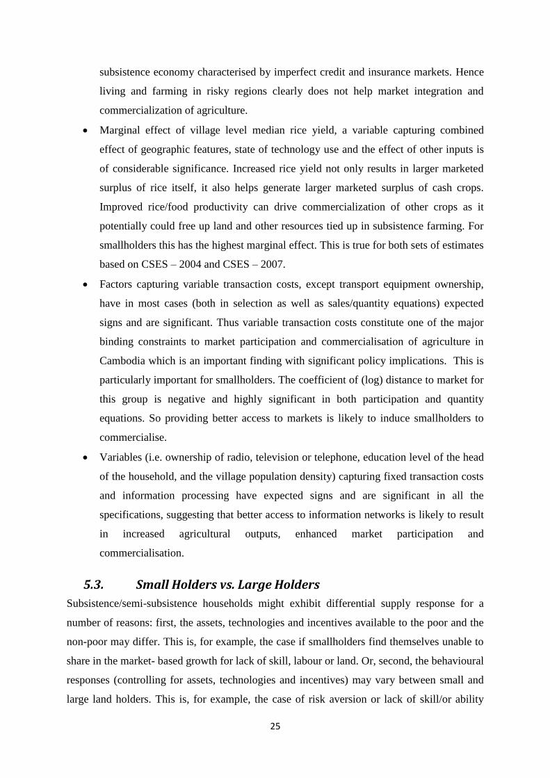
Figure 4 compares unconditional marginal effects of small and large holders for all crop

categories. Clearly, the differences between the marginal effects of small and large holders

are substantial.

Figure 4 Marginal Effects of Small vs Large Holders

5.4. Estimates Based on CSES – 2007 Data

Table 7 gives the regression results based on CSES – 2007 data for all households and the

corresponding unconditional marginal effects are reported in figure 5 and in appendix 2. As

before, for each model there are two columns – the first column (quantity) reports the log of

annual sales given market participation and the second column (select) shows the results of

market participation probability model.

31

Table 7 Regression Results (CSES-2007), Dependent Variable = log Sales value of marketed Surplus Food Crops Cash Crops All Crops

Variables Quantity Select Quantity Select Quantity Select

Log median price of paddy (vill) 0.0148 0.175***

-0.109* 0.0782

*** -0.0781

** 0.0640

**

(0.42) (8.04) (-2.37) (4.13) (-3.22) (3.16)

Log land per worker 0.687***

0.584***

0.181**

0.0404 0.635***

0.436***

(10.15) (15.86) (2.61) (1.33) (13.09) (13.40)

Log age of HH 0.00170 0.000336 -0.00669 0.00770**

0.00194 0.00267

(0.50) (0.13) (-1.08) (3.03) (0.64) (1.03)

Dependency ratio -0.513***

-0.421***

-0.143 -0.0392 -0.461***

-0.353***

(-6.46) (-8.00) (-1.22) (-0.77) (-6.86) (-6.93)

Dummy for land title 0.238* 0.0729 -0.170 0.123 0.148 0.139

(2.35) (1.00) (-0.99) (1.71) (1.69) (1.93)

Dummy for paid job 0.124 -0.142 -0.269 0.0622 0.0116 -0.108

(1.21) (-1.93) (-1.65) (0.87) (0.13) (-1.48)

Dummy for risky region -0.104 -0.0971 0.104 0.137 0.0728 0.0644

(-0.97) (-1.27) (0.59) (1.83) (0.80) (0.85)

Log median rice yield (vill) 1.388***

0.983***

0.157 0.0636 1.194***

0.809***

(10.49) (12.16) (0.96) (0.89) (11.41) (10.75)

Dummy for ownership of ag. Implements 0.134 -0.0260 -0.431* 0.177

* 0.150 -0.0389

(1.14) (-0.30) (-2.10) (2.06) (1.45) (-0.45)

Dummy for ethnicity 0.589 0.358 -1.519* 0.160 -0.487 0.507

*

(1.52) (1.42) (-2.34) (0.62) (-1.36) (2.15)

Dummy for transport equipments 0.0166 0.326***

0.162 0.126 0.0582 0.352***

(0.14) (3.55) (0.77) (1.41) (0.54) (3.77)

Log distance to provincial capital -0.120* -0.111

** 0.0811 -0.0719 -0.0565 -0.0764

(-2.48) (-3.17) (1.05) (-1.37) (-1.37) (-1.41)

Log distance to bus stop 0.178* 0.0586 -0.149 -0.145

** 0.0633 -0.0397

(2.38) (1.08) (-1.21) (-2.74) (0.98) (-0.74)

Log distance to market -0.0457 -0.0149 0.420***

0.0631 0.0164 -0.0251

(-0.61) (-0.27) (3.44) (1.84) (0.26) (-0.72)

Dummy for radio, TV, or telephone 0.273* -0.0710 0.155

(2.46) (-0.81) (1.39)

Log village population density -0.0956***

0.0610**

-0.0309

(-3.77) (3.10) (-1.24)

Educational level of HH 0.0236* 0.0132 0.0248

*

(2.08) (1.38) (2.21)

Constant 12.16 -0.570 16.46 -0.904 13.87 -0.0210

(20.15) (-1.32) (17.05) (-2.19) (27.51) (-0.05)

Number of Observations 1698 1698 1698

t statistics in parentheses* p < 0.05,

** p < 0.01,

*** p < 0.001

5.5. Summary of Results

All households:

For market participation decision – the coefficients for log price of rice are positive

and highly significant in all three models. However, for all quantity equations they are

32

negative and significant for cash crops. For food crops it is still positive but non-

significant. The marginal effects seem to be weaker compared to the estimates based on

CSES – 2004 data. This could be due to the fact that the sample size for CSES – 2007 is

much smaller than that of CSES – 2004 and that there is very little price variation in the

data.

The coefficients for the capital endowment variable – land per worker – are positive

and significant for both quantity and market participation equations indicating that

relatively well-endowed farmers participate in the market and commercialize. This is

completely in line with the initial estimates based on CSES – 2004 data. The marginal

effects for this variable are also the second largest, implying that for generating

marketable surpluses and commercialization of agriculture in Cambodia land

redistribution/allocation has significant policy implications.

Among the household background characteristic variables – dependency ratio has the

expected sign in all the models and is highly significant. The Cambodian population is

relatively young and the higher dependency ratio seems to be a deterrent for generating

marketable agricultural surpluses and commercialization as suggested by the size of the

marginal effect for this variable (largest negative). Other background variables such as

‘Log of age of head of household’ and ‘any member has paid job’ have the expected

signs, but are non-significant in most cases.

Geographical features such as median village rice yield per hectare, dummy for risky

region in most cases (in both market participation and quantity equations) have the

expected signs and are significant. So improved rice/food productivity can drive

commercialization of other crops as it potentially could free up land and other resources

tied up in subsistence farming.

Variables capturing transaction costs (both fixed and variable) have in most cases

similar estimates as with CSES – 2004 data in terms of the sign and size of the

coefficients and marginal effects. Ownership of transport equipment, and distance

variables have in most cases expected signs and are significant, indicating that measures

to reduce transactions costs could help farmers to produce beyond subsistence level.

Similarly, variables such as ownership of radio, TV or telephone, village population

density, and the educational level of head of household, which are expected to capture

fixed transaction costs and information processing, all have sizeable marginal effects.

33

Figure 5 Marginal Effects - All (CSES- 2007)

5.6. Small vs. Large Holders

As with the case of all households, regression results and the corresponding marginal effects

for small and large holders based on CSES – 2007 data are largely in line with our initial

estimates based on CSES – 2004 data. The main findings are highlighted below:

Results based on CSES – 2007 are largely similar to our initial estimates based on

CSES – 2004. As revealed by the regression results in table 8 and 9, and the

corresponding marginal effects in fig. 6 and 7, variables such as price of paddy, rice yield

(capturing the state of technology use), land per worker, and land title continue to have

similar positive and significant marginal effects, with notable differences between small

and large holders’ responses. Price of paddy is no longer the dominant determinant of

supply response; however, it remains the case that for small holders it is far less important

for commercial production of agricultural outputs than for large holders. Similarly, land

title, transaction costs variables, capital endowment and household background

characteristics such as land per worker and ethnicity are far more important to

smallholders than to large holders.

Transaction costs continue to be one of the main barriers for generating marketed

surplus of food crops for small/subsistence holders. Variables capturing variable

transaction costs, that is, distance to market, distance to bus stop, distance to provincial

capital and ownership of transport equipments all have the expected signs and significant

marginal effects on supply response. However, the same is not true for large holders.

34

Similarly, the land title variable has sizeable and significant positive marginal effects,

consistent with our earlier findings with CSES – 2004 data. Thus, it is safe to argue that

secure land ownership facilitates market integration of subsistence farmers in Cambodia.

Table 8 Regression Results (CSES – 2007; Small holders), Dependent Variable = log Sales value of

marketed Surplus Food Crops Cash Crops All Crops

Variables Quantity Select Quantity Select Quantity Select

Log median price of paddy (vill) -0.237*** 0.128*** -0.150* -0.0899*** -0.155*** 0.0153 (-3.40) (4.61) (-2.44) (-3.64) (-3.60) (0.66) Log land per worker 0.623*** 0.390*** 0.227* -0.0920 0.0700 0.19*** (4.46) (7.64) (2.34) (-1.91) (0.83) (4.35) Log age of HH 0.0113 -0.00114 -0.0094 0.00495 -0.000184 0.0028 (1.50) (-0.35) (-1.27) (1.35) (-0.03) (0.89) Dependency ratio 0.227 -0.291*** -0.179 0.00823 -0.00415 -0.20** (1.29) (-4.15) (-1.29) (0.11) (-0.03) (-3.13) Dummy for land title 0.0757 0.189 0.0879 0.213 0.217 0.150 (0.32) (1.90) (0.38) (1.96) (1.21) (1.63) Dummy for paid job -0.0222 -0.162 -0.0351 0.0940 -0.00477 -0.0874 (-0.10) (-1.69) (-0.18) (0.91) (-0.03) (-0.97) Dummy for risky region 0.185 -0.139 -0.426 0.195 -0.124 0.0221 (0.74) (-1.33) (-1.64) (1.68) (-0.64) (0.23) Log median rice yield (vill) 0.549 0.925*** 0.670* 0.329** 0.108 0.84*** (1.69) (7.68) (2.19) (2.69) (0.46) (7.86) Dummy for ownership of ag. Implements 0.350 -0.0671 -0.125 0.374** 0.254 -0.0021 (1.22) (-0.56) (-0.38) (2.87) (1.15) (-0.02) Dummy for ethnicity -0.125 1.126* -0.397 -0.183 -1.770* 0.590 (-0.08) (2.02) (-0.52) (-0.48) (-1.97) (1.57) Dummy for transport equipments -0.643* 0.299* 0.0533 -0.0582 -0.442 0.216 (-1.97) (2.20) (0.19) (-0.39) (-1.74) (1.66) Log distance to provincial capital 0.0900 -0.116* -0.0904 -0.0967 0.0291 -0.0621 (0.68) (-2.27) (-0.78) (-1.32) (0.30) (-1.31) Log distance to bus stop 0.367 0.0608 0.167 -0.176* 0.430** -0.0619 (1.95) (0.80) (0.88) (-2.08) (3.07) (-0.87) Log distance to market -0.0981 0.0111 0.363* 0.0996 0.0725 -0.0082 (-0.58) (0.16) (2.52) (1.75) (0.59) (-0.13) Dummy for radio, TV, or telephone 0.349** -0.202 0.165 (2.84) (-1.21) (1.40) Log village population density -0.0393 0.0403 -0.0084 (-1.39) (1.19) (-0.34) Educational level of HH 0.0203 0.0266 0.0259* (1.79) (1.79) (2.45) Constant 14.18 -1.936 13.71 -0.995 15.32 -0.879 (7.56) (-2.69) (10.20) (-1.60) (13.59) (-1.58)

Number of Observations 917 917 917

t statistics in parentheses * p < 0.05,

** p < 0.01,

*** p < 0.001

35

Table 9 Regression Results (CSES 2007 – Large holders), Dependent Variable = log Sales value of

marketed Surplus

Food Crops Cash Crops All Crops

Variables Quantity Select Quantity Select Quantity Select

Log median price of paddy (vill) 0.00844 0.216*** -0.123 -0.061* -0.0293 0.178***

(0.15) (6.32) (-1.67) (-1.97) (-0.91) (4.85)

Log land per worker 0.769*** 0.651*** 0.390 -0.128 0.782*** 0.496***

(6.50) (7.21) (1.90) (-1.61) (10.41) (5.06)

Log age of HH -0.00337 -0.00128 -0.00615 0.011** 0.00230 -0.00017

(-0.92) (-0.30) (-0.65) (2.74) (0.67) (-0.03)

Dependency ratio -0.435*** -0.434*** -0.136 0.0350 -0.471*** -0.429***

(-4.15) (-5.19) (-0.75) (0.46) (-6.20) (-4.76)

Dummy for land title 0.141 -0.0241 -0.195 0.0460 -0.0185 0.183

(1.40) (-0.22) (-0.80) (0.45) (-0.19) (1.53)

Dummy for paid job 0.242* -0.101 -0.395 -0.0509 0.0664 -0.170

(2.33) (-0.90) (-1.60) (-0.49) (0.67) (-1.36)

Dummy for risky region -0.00751 -0.0419 0.394 0.0693 0.240* 0.0964

(-0.07) (-0.37) (1.60) (0.67) (2.48) (0.75)

Log median rice yield (vill) 1.512*** 0.969*** 0.265 -0.0847 1.346*** 0.812***

(7.78) (8.45) (1.14) (-0.90) (13.64) (7.05)

Dummy for ag. Implements 0.0479 0.0166 -0.244 -0.0066 -0.0158 -0.243

(0.42) (0.13) (-0.82) (-0.05) (-0.14) (-1.57)

Dummy for ethnicity 0.387 -0.0247 -2.299* 0.425 -0.648 0.333

(1.20) (-0.07) (-2.40) (1.13) (-1.92) (0.96)

Dummy for transport equipments 0.0352 0.288* 0.194 0.0721 0.109 0.327*

(0.29) (2.26) (0.68) (0.62) (1.01) (2.28)

Log distance to provincial capital -0.0981* -0.0456 0.203* -0.0082 -0.0508 -0.101

(-2.19) (-0.52) (1.97) (-0.10) (-1.22) (-1.00)

Log distance to bus stop 0.00786 0.0221 -0.327 -0.181** -0.150* -0.141

(0.11) (0.29) (-1.93) (-2.58) (-2.22) (-1.64)

Log distance to market 0.00261 -0.0933 0.247 0.0708 0.0573 0.0445

(0.03) (-1.87) (1.28) (1.55) (0.78) (0.80)

Dummy for radio, TV, or telephone 0.218 -0.102 0.00289

(1.40) (-0.93) (0.02)

Log village population density -0.120** 0.098*** -0.0433

(-2.78) (3.63) (-0.95)

Educational level of HH 0.00625 0.0110 0.0129

(0.35) (0.78) (0.63)

Constant 12.93 0.175 18.15 -1.366 14.27 0.471

(19.26) (0.27) (13.00) (-2.31) (27.08) (0.68)

Number of Observations 781 781 781

t statistics in parentheses * p < 0.05,

** p < 0.01,

*** p < 0.001

36

Figure 6 Marginal Effects - Small Holders (CSES - 2007)

Figure 7 Marginal Effects - Large Holders (CSES - 2007)

37

6. Conclusion

Using household survey data of Cambodia (CSES – 2004 and CSES – 2007), this study

assessed the effects of transactions costs as well as price and non-price factors on market

participation and marketed surplus. A switching regression model was used that accounts not

only for the effects of fixed and variable transactions costs but also for the role of

heterogeneous endowments, technology, and other institutional factors in promoting market

participation and generating marketable surpluses. In doing so, we estimated the model for

three crop types and the same regressions for smallholders - who are most likely to be among

the poorest and the most vulnerable – as well as large holders. We estimated the

unconditional marginal effects, that is, the total change in quantities transacted unconditional

on market participation, for the full sample and for the samples of small and large holders.

Some of our findings we believe could be very useful for future policy design for poverty

alleviation and small/subsistence holder’s welfare.

Comparison between the marginal effects of the small and large holders reveals substantial

qualitative and quantitative differences between these two groups. By providing technical

support/ extension services and resolving land issues and land redistribution, targeted support

in the form of basic agricultural assets can have high payoffs in terms of poverty alleviation,

reduced vulnerability and increased food security. Furthermore, targeted support helps the

poor to participate in the growth process and to reap benefit out of the opportunities opened

up by the exchange economy. Having secure land title is important for poverty alleviation

and reducing vulnerability through increased participation of smallholders and subsistence

farmers in markets and commercial sales.

Integrating non-ethnic Khmers into the mainstream of economic activities is also likely to

payoff in terms of poverty alleviation and a vibrant rural economy. Another important finding

is the transaction cost barrier for smallholders’ market participation. Easier access of

smallholders to better rural infrastructure (e.g. road networks and other physical facilities) is

important for producing outputs to meet market demand. Evidence points to geographic

poverty traps that are exacerbated by risk aversion and low-return crops, causing poverty to

persist for generations. High yielding varieties, extension services along with insurance

would help in breaking out of the shackles of subsistence farming.

38

Overall, the findings suggest that policy options other than price policies are available to

promote commercialization and generate agricultural surpluses, particularly by the

smallholders. This is important because, in the short run, higher prices are likely to benefit

sellers (mostly large holders who are already in the market) only, impose costs on buying

households unable to respond to price incentives, and bypass those failing to participate in

markets because of high transactions costs and other barriers to market entry. Therefore, price

policies will have very different behavioural and welfare implications for different segments

of the farming population. In the face of the food price dilemma facing many countries

recently, policies that reduce transactions costs and induce smallholders to commercialize

could thus be important alternatives to price policies to promote marketed surplus and

commercialization of agriculture by smallholders and thereby reduce poverty and

vulnerability of this particular community of farmers.

39

References

Abdulai, A., and C. L. Delgado. “Determinants of Nonfarm Earnings of Farm-based Husband

and Wives in Northern Ghana.” American Journal of Agricultural Economics, 81 , 1999:

117-130.

Acker, Van Frank. Hitting a Stone with an Egg? Cambodia's Rural Economy and Land

Tenure in Transition. CAS Discussion Paper No. 23, Centre for Asian Studies, 1999.

ADB. Cambodia: Country Poverty Analysis. Manila: Asian Development Bank, 2011.

Askari H., and Cummings, J. “Output price response in agriculture: an evaluation.” Indian

Journal of Agricultural Economics, Vol.29, 1974: 165-174.

Askari, H., and J. T. Cummings. Agricultural Supply Response: A Survey of the Econometric

Evidence. London: Praeger, 1976.

Bardhan, K. “Price and output response of marketed surplus of foodgrains: a cross-sectional

study of some North Indian villages.” Ameriacal Journal of Agricultural Economics, Vol.52,

1970: 51-61.

Barnum, H. N., and L. Squire. A Model of an Agricultural Household: Theory and Evidence.

World Bank Staff Occasional Paper, No. 27 , Baltimore: Johns Hopkins University Press,

1979.

Barnum, H., and Squire, L. “An econometric application of the theory of the farm household.”

Journal of Development Economics, Vol.6, 1979: 79-102.

Barrett, C. B. “Smallholder Market Participation: Concepts and Evidence from Eastern and

Southern Africa.” Food Policy,33, 2008: 299-317.

Benjamin, Dwayne. “Household Composition, Labor Markets, and Labor Demand: Testing

for Separation in Agricultural Household Models.” Econometrica, 60(2), 1992: 287-322.

Brooks, Jonathan, George Dyer, and Ed Taylor. Modelling Agricultural Trade and Policy

Impacts in Less Developed Countries. OECD Food, Agriculture and Fisheries Working Paper,

No. 11, OECD Publishing, 2008.

Cadot, Olivier, L. Dutoit, and M. Olarreaga. The Cost of Moving Out of Subsistence. Mimeo,

University of Lausanne, 2006.

Carter, M. R., and Y. Yao. “Local versus Global Separability in Agricultural Household

Models: The Factor Price Equalization Effects of Land Transfer Rights.” American Journal

of Agricultural Economics, 69, 2002: 369-377.

Chayanov, A. V. The Theory of Peasant Economy. Translated by D. Thorner, B. Kerblay and

R. E. F. Smith. D. Irwin: Homewood, IL, 1925.

40

Christian H.C.A. Henning, and Arne Henningsen. “Modeling Farm Household's Price

Responses in the Presence of Transaction Costs and Heterogeneity in Labor Markets.”

American Journal of Agricultural Economics, Vol.89, No.3, 2007: 665-681.

de Janvry, A., and E. Sadoulet. “Progress in the Modeling of Rural Households' Behavior

under Market Failures .” In Poverty, Inequality and Development, Essays in Honor of Erik

Thorbecke, by A. de Janvry and R. Kanbur, Chapter 8. Kluwer Publishing, 2006.

de Janvry, Alain, Marcel Fafchamps, and Elisabeth Sadoulet. “Peasant Household Behavior

with Missing Markets: Some Paradoxes Explained.” Economic Journal, 101(409), 1991:

1400-17.

Enke, S. Economics for Development. Englewood Cliffs: Prentice Hall, 1963.

Eswaran, M., and A. Kotwal. “Implications of Credit Constraints for Risk Behaviour in less

Developed Economies.” Oxford Economics Papers, 42(2), 1990: 473-482.

Fafchamps, M, C Udry, and K Czukas. “Drought and Saving in West Africa: Are Livestock a

Buffer Stock?” Journal of Development Economics, 1998: 55(2): 273-305.

Goetz, Stephan J. “A Selectivity Model of Household Food Marketing Behaviour in Sub-

Saharan Africa.” American Journal of Agricultural Economics, Vol. 74, No. 2, May, 1992:

444-452.

Haessel, W. “The price and income elasticities of home consumption and marketed surplus of

food grains.” American Journal of Agricultural Economics, Vol.57, 1975: 111-115.

Heltberg, R., and F. Tarp. “Agricultural Supply response and poverty in Mozambique.” Food

Policy, Vol.27, 2002: 103-124.

Hoffmann, R., and A., L. Kassouf. “Deriving Conditional and Unconditional Marginal

Effects in log Earning Equations Estimated by Heckman's Procedure.” Taylor and Francis

Journasl, Vol.31(11), 2005: 1303-1311.

Huang, C.L., R. Raunikar, and Misra. “The application and economic interpretation of

selectivity models.” American Journal of Agricultutral Economics, Vol.73, No.2, 1991: 496-

501.

Jayne, T. S., D. Mather, and E. Mghenyi. “Principal Challenges Confronting Smallholder

Agricultural Households in Sub-Saharan Agriculture.” World Development, 38(10), 2010:

1384-1398.

Key, N., E. Sadoulet, and A. de Janvry. “Transaction Costs and Agricultural Household

Supply Response.” American Journal of Agricultural Economics, 82(May), 2000: 245-259.

Krishna, R. “Agricultural price policy and economic development.” In Agricutural

Development and Economic Growth, by H Southworth and B Johnston, 497-540. Ithaca, NY:

Cornell University Press, 1967.

41

Krishnan, T. N. “The Marketed Surplus of Foodgrains: Is it Inversely Related to Price?”

Economic Weekly, Annual No. 17, 1965.

Maddala, G. S. Limited Dependent and Qualitative Variables in Econometrics. Cambridge:

Cambridge University Press, 1983.

Mathur, P. N., and H. Ezekiel. “Marketable Surplus of Food and Price Fluctuations in a

Developing Economy.” Kyklos, 14, 1961: 396-408.

Nowshirvani, V. F. “A Note on the Fixed-cash-requirement Theory of Marketed Surplus in

Subsistence Agriculture.” Kyklos, 20, 1967: 772-773.

Olson, R. O. “Impact and Implications of Foreign Surplus Disposal on Underdeveloped

Countries.” Journal of Farm Economics, 42, 1960: 1042-1051.

Ozanne, Adam. “Perverse supply response in peasant agriculture: A review.” Oxford

Development Studies, Vol.27, No.2, 1999: 251-270.

Paxson, C. H. “Using Weather Variability to Estimate the Response of Savings to Transitory

Income in Thailand.” The American Economic Review, 82(1), 1992: 15-33.

Rao, J. Mohan. “Agricultural Supply Response: A Survey.” Agricultural Economics, Vol.3,

1989: 1-22.

Sadoulet, E., A. de Janvry, and C. Benjamin. “Household Behavior with Imperfect Labor

Market.” Industrial Relations, 37(1), 1998: 85-108.

Sadoulet, E., and A. de Janvry. Quantitative development policy analysis. Baltimore and

London: The Johns Hopkins University Press, 1995.

Sharma, K. L., and M. P. Gupta. “Study of Farm Factors Determining Marketed Surplus of

Bajra in Jaipur District.” Indian Journal of Agricultural Economics, No.25, 1970: 64-68.

Sigelman, L., and L. Zeng. “Analyzing censored and sampled-selected data with Tobit and

Heckit models.” Political Analysis, Vol. 8, 1999: 167-182.

Singh, I., Lynn Squire, and John Strauss. Agricultural Household Models. Baltimore. MD:

The Johns Hopkins University Press, 1986.

Singh, Inderjit, Lyn Squire, and John Strauss. “A Survey of Agricultural Household Models:

Recent Findings and Policy Implications.” The World Bank Economic Review, Vol.1, No.1,

1986: 149-179.

Skoufias, Emmanuel. “Using Shadow Wages to Estimate Labor Supply of Agricultural

Households.” American Journal of Agricultural Economics, 76(2), 1994: 215-227.

Strauss, John. “Does better Nutrition Raise Farm Productivity?” Journal of Political

Economy, 94(2), 1986: 297-320.

42

Strauss, John. “Marketed Surpluses of Agricultural Households in Sierra Leone.” American

Journal of Agricultural Economics, Vol.66 No.3, Aug. 1984: 321-331.

Vance, C., and J. Geoghehan. “Modeling the Determinants of Semi-Subsistent and

Commercial Land Uses in an Agricultural Frontier of Southern Mexico: A Switching

Regression Approach.” International Regional Science Review, 27, 2004: 326-347.

43

Appendix 1

Marginal Effects

There are four different responses of marketing behaviour to changes in explanatory variables

in selectivity models (Huang et al. 1991). These are: i) the change in probability of marketing

participation; ii) the change in desired quantities traded; iii) the change in actual quantities

traded conditional on market participation; and iv) the total change in quantities transacted

unconditional on market participation. The unconditional marginal effect, which is of

particular interest for this study, on actual quantities transacted ( ) per unit change in the

variable can be calculated as (Huang et al. 1991) follows:

(15)

where, and correspond to the estimated parameters for variable in the quantity and

selection equation of the model respectively; while, and stand for cumulative and

probability density functions of standard normal distribution respectively. The above

equation shows that the total unconditional marginal effect on quantities transacted equals the

sum of (1) the marginal effect on quantities transacted by participants weighted by the

probability of participation, and (2) the marginal effect on the probability of participation

weighted by the expected quantities transacted by participants. While the changes in the

quantities transacted by participants weighted by probability of participation represent the

total effects due to current participants, the changes in probability of participation weighted

by expected quantities transacted by participants represents total effects due to new

participants.

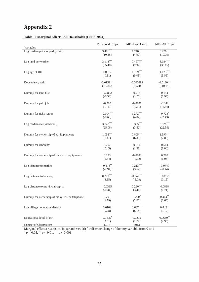
44

Appendix 2

Table 10 Marginal Effects: All Households (CSES-2004)

ME - Food Crops ME - Cash Crops ME - All Crops

Variables

Log median price of paddy (vill) 3.486*** 1.246*** 3.726***

(10.68) (4.90) (10.79)

Log land per worker 3.113*** 0.497*** 3.034***

(35.48) (7.97) (33.15)

Log age of HH 0.0912 1.199*** 1.123***

(0.31) (5.03) (3.56)

Dependency ratio -0.0159*** -0.000693 -0.0130***

(-12.85) (-0.74) (-10.19)

Dummy for land title -0.0832 0.216 0.154

(-0.53) (1.76) (0.93)

Dummy for paid job -0.290 -0.0181 -0.342

(-1.40) (-0.11) (-1.54)

Dummy for risky region -2.004*** 1.272*** -0.723*

(-8.68) (4.84) (-2.43)

Log median rice yield (vill) 3.748*** 0.385*** 3.528***

(25.06) (3.52) (22.59)

Dummy for ownership of ag. Implements 1.052*** 0.805*** 1.390***

(6.41) (6.33) (7.86)

Dummy for ethnicity 0.207 0.514 0.514

(0.43) (1.51) (1.00)

Dummy for ownership of transport equipments 0.293 -0.0188 0.210

(1.54) (-0.12) (1.04)

Log distance to market -0.218** 0.213*** -0.0349

(-2.94) (3.62) (-0.44)

Log distance to bus stop 0.270*** -0.342*** 0.00955

(4.85) (-8.09) (0.16)

Log distance to provincial capital -0.0385 0.290*** 0.0838

(-0.34) (3.41) (0.71)

Dummy for ownership of radio, TV, or telephone 0.291 0.290* 0.464**

(1.79) (2.26) (2.68)

Log village population density 0.0109 0.637*** 0.445**

(0.08) (6.14) (3.19)

Educational level of HH 0.0475* 0.0295 0.0630**

(2.31) (1.79) (2.90)

Number of Observations 6913 6913

Marginal effects; t statistics in parentheses (d) for discrete change of dummy variable from 0 to 1 * p < 0.05,

** p < 0.01,

*** p < 0.001

45

Table 11 Marginal Effects: Small Holders (CSES-2004)

ME - Food Crops ME - Cash Crops ME - All crops

Log median price of paddy (vill) 2.596*** 0.614* 2.832***

(7.71) (2.18) (7.01)

Log land per worker 1.619*** 0.139 1.594***

(17.15) (1.96) (14.51)

Log age of HH -0.417 0.539* 0.213

(-1.41) (2.10) (0.60)

Dependency ratio -0.00943*** -0.000958 -0.00912***

(-7.58) (-0.95) (-6.30)

Dummy for land title -0.107 0.389** 0.280

(-0.66) (2.88) (1.44)

Dummy for paid job -0.339 -0.0629 -0.382

(-1.67) (-0.37) (-1.55)

Dummy for risky region -1.080*** 0.985** -0.176

(-4.50) (3.28) (-0.51)

Log median rice yield (vill) 2.554*** 0.769*** 3.066***

(17.47) (6.58) (17.26)

Dummy for ownership of ag. Implements 0.575*** 0.609*** 0.932***

(3.52) (4.49) (4.79)

Dummy for ethnicity 0.178 0.609 0.920

(0.36) (1.82) (1.67)

Dummy for ownership of transport equipments 0.151 -0.0746 0.0651

(0.80) (-0.46) (0.29)

Log distance to market -0.282*** 0.0368 -0.251**

(-3.58) (0.56) (-2.67)

Log distance to bus stop 0.244*** -0.182*** 0.0514

(4.15) (-3.91) (0.75)

Log distance to provincial capital -0.179 0.0229 -0.174

(-1.56) (0.25) (-1.30)

Dummy for ownership of radio, TV, or telephone -0.00907 0.214 0.170

(-0.05) (1.55) (0.82)

Log village population density -0.117 0.457*** 0.221

(-0.86) (4.06) (1.36)

Educational level of HH 0.00149 -0.00646 -0.00360

(0.17) (-0.84) (-0.34)

Number of Observations 3982 3982

Marginal effects; t statistics in parentheses (d) for discrete change of dummy variable from 0 to 1 * p < 0.05,

** p < 0.01,

*** p < 0.001

46

Table 12 Marginal Effects: Large Holders (CSES – 2004)

ME - Food Crops ME - Cash Crops ME - All Crops

Log median price of paddy (vill) 4.697***

2.362***

4.683***

(8.58) (5.18) (9.78)

Log land per worker 3.623***

-0.541**

2.103***

(16.09) (-2.96) (10.43)

Log age of HH 0.0716 1.033* 0.397

(0.14) (2.36) (0.86)

Dependency ratio -0.0192***

0.00456* -0.00910

***

(-8.94) (2.53) (-4.79)

Dummy for land title 0.0137 0.0786 0.0456

(0.05) (0.36) (0.20)

Dummy for paid job 0.107 0.0341 0.0109

(0.31) (0.12) (0.03)

Dummy for risky region -2.854***

1.852***

-1.126*

(-6.27) (4.04) (-2.54)

Log median rice yield (vill) 4.552***

0.00944 3.270***

(17.52) (0.05) (14.37)

Dummy for ownership of ag. Implements 0.875**

0.373 0.591*

(2.75) (1.38) (2.00)

Dummy for ethnicity 1.039 0.604 0.505

(1.28) (0.96) (0.67)

Dummy for ownership of transport

equipments

-0.0906 -0.262 -0.405

(-0.27) (-0.90) (-1.42)

Log distance to market -0.107 0.328**

0.135

(-0.89) (3.17) (1.25)

Log distance to bus stop 0.192* -0.561

*** -0.0212

(2.12) (-7.36) (-0.26)

Log distance to provincial capital 0.0874 0.578***

0.115

(0.46) (3.66) (0.69)

Dummy for ownership of radio, TV, or

telephone

0.983***

0.353 1.179***

(4.07) (1.54) (4.90)

Log village population density 0.366 0.789***

0.969***

(1.82) (4.14) (4.96)

Educational level of HH 0.0259* 0.0130 0.0160

(2.06) (1.34) (1.41)

Number of Observations 2996 2996

Marginal effects; t statistics in parentheses (d) for discrete change of dummy variable from 0 to 1 * p < 0.05,

** p < 0.01,

*** p < 0.001

47

Table 13 Marginal Effects: All Households (CSES-2007)

ME - Food Crops ME- Cash Crops ME- All

Crops

Variables

Log median price of paddy (vill) 0.911***

-0.371***

0.249*

(8.03) (-4.73) (2.55)

Log land per worker 3.356***

0.223 2.484***

(17.58) (1.77) (16.07)

Log age of HH 0.00257 0.0322**

0.0139

(0.19) (3.07) (1.11)

Dependency ratio -2.427***

-0.209 -1.972***

(-8.86) (-0.99) (-8.07)

Dummy for land title 0.492 0.496 0.757*

(1.30) (1.69) (2.17)

Dummy for paid job -0.672 0.206 -0.502

(-1.76) (0.69) (-1.42)

Dummy for risky region -0.553 0.627* 0.353

(-1.38) (2.05) (0.96)

Log median rice yield (vill) 5.762***

0.319 4.616***

(13.70) (1.08) (12.88)

Dummy for ownership of ag. Implements -0.0691 0.667 -0.0819

(-0.15) (1.90) (-0.20)

Dummy for ethnicity 2.014 0.345 2.331

(1.72) (0.33) (1.80)

Dummy for ownership of transport equipments 1.686***

0.607 1.644***

(3.57) (1.59) (3.92)

Log distance to provincial capital -0.0995 -0.210 -0.349

(-0.34) (-0.97) (-1.33)

Log distance to bus stop 0.390 -0.673**

-0.144

(1.38) (-3.09) (-0.56)

Log distance to market -0.635***

0.298* -0.157

(-3.47) (2.11) (-0.93)

Dummy for ownership of radio, TV, or telephone 1.403* -0.305 0.710

(2.48) (-0.83) (1.43)

Log village population density -0.494***

0.268**

-0.145

(-3.75) (3.14) (-1.24)

Educational level of HH 0.122* 0.0582 0.117

*

(2.07) (1.39) (2.20)

Number of Observations 1698 1698 1698

Marginal effects; t statistics in parentheses (d) for discrete change of dummy variable from 0 to 1 * p < 0.05,

** p < 0.01,

*** p < 0.001

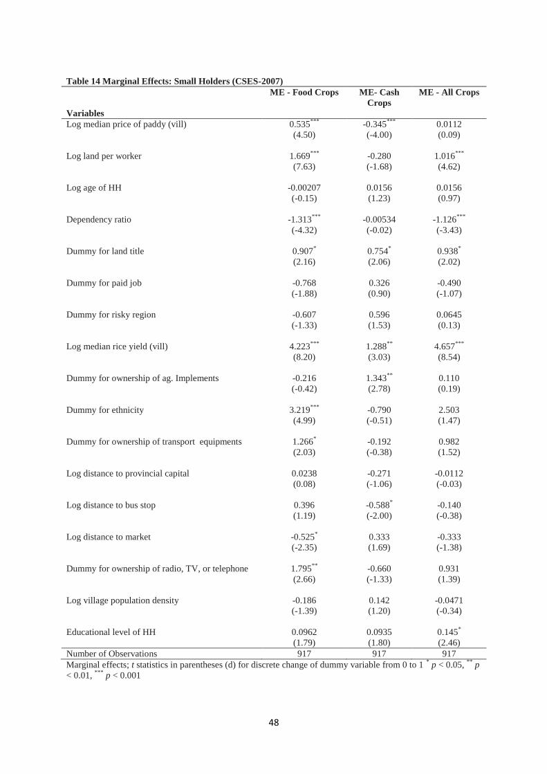
48

Table 14 Marginal Effects: Small Holders (CSES-2007)

ME - Food Crops ME- Cash

Crops

ME - All Crops

Variables

Log median price of paddy (vill) 0.535***

-0.345***

0.0112

(4.50) (-4.00) (0.09)

Log land per worker 1.669***

-0.280 1.016***

(7.63) (-1.68) (4.62)

Log age of HH -0.00207 0.0156 0.0156

(-0.15) (1.23) (0.97)

Dependency ratio -1.313***

-0.00534 -1.126***

(-4.32) (-0.02) (-3.43)

Dummy for land title 0.907* 0.754

* 0.938

*

(2.16) (2.06) (2.02)

Dummy for paid job -0.768 0.326 -0.490

(-1.88) (0.90) (-1.07)

Dummy for risky region -0.607 0.596 0.0645

(-1.33) (1.53) (0.13)

Log median rice yield (vill) 4.223***

1.288**

4.657***

(8.20) (3.03) (8.54)

Dummy for ownership of ag. Implements -0.216 1.343**

0.110

(-0.42) (2.78) (0.19)

Dummy for ethnicity 3.219***

-0.790 2.503

(4.99) (-0.51) (1.47)

Dummy for ownership of transport equipments 1.266* -0.192 0.982

(2.03) (-0.38) (1.52)

Log distance to provincial capital 0.0238 -0.271 -0.0112

(0.08) (-1.06) (-0.03)

Log distance to bus stop 0.396 -0.588* -0.140

(1.19) (-2.00) (-0.38)

Log distance to market -0.525* 0.333 -0.333

(-2.35) (1.69) (-1.38)

Dummy for ownership of radio, TV, or telephone 1.795**

-0.660 0.931

(2.66) (-1.33) (1.39)

Log village population density -0.186 0.142 -0.0471

(-1.39) (1.20) (-0.34)

Educational level of HH 0.0962 0.0935 0.145*

(1.79) (1.80) (2.46)

Number of Observations 917 917 917

Marginal effects; t statistics in parentheses (d) for discrete change of dummy variable from 0 to 1 * p < 0.05,

** p

< 0.01, ***

p < 0.001

49

Table 15 Marginal Effects: Large Holders (CSES-2007)

ME - Food Crops ME - Cash Crops ME- All Crops

Variables

Log median price of paddy (vill) 0.999***

-0.344* 0.487

***

(6.40) (-2.40) (4.45)

Log land per worker 3.547***

-0.521 2.110***

(8.58) (-1.40) (7.30)

Log age of HH -0.00834 0.0509**

0.00152

(-0.42) (2.87) (0.11)

Dependency ratio -2.310***

0.134 -1.647***

(-6.09) (0.38) (-6.10)

Dummy for land title -0.00792 0.170 0.520

(-0.02) (0.36) (1.41)

Dummy for paid job -0.299 -0.376 -0.451

(-0.56) (-0.80) (-1.12)

Dummy for risky region -0.198 0.472 0.486

(-0.38) (0.99) (1.26)

Log median rice yield (vill) 5.548***

-0.343 3.512***

(10.87) (-0.78) (10.53)

Dummy for ownership of ag. Implements 0.111 -0.110 -0.687

(0.18) (-0.19) (-1.60)

Dummy for ethnicity 0.171 1.412 0.627

(0.11) (0.97) (0.42)

Dummy for ownership of transport

equipments

1.334* 0.425 1.025

*

(2.33) (0.79) (2.44)

Log distance to provincial capital -0.208 0.0360 -0.242

(-0.51) (0.10) (-0.80)

Log distance to bus stop 0.107 -1.015**

-0.538*

(0.30) (-3.15) (-2.07)

Log distance to market -0.499* 0.420

* 0.0842

(-2.16) (2.00) (0.51)

Dummy for ownership of radio, TV, or

telephone

0.956 -0.501 0.00832

(1.47) (-0.95) (0.02)

Log village population density -0.553**

0.493***

-0.125

(-2.66) (3.71) (-0.96)

Educational level of HH 0.0287 0.0556 0.0374

(0.35) (0.78) (0.63)

Number of Observations 781 781 781

Marginal effects; t statistics in parentheses (d) for discrete change of dummy variable from 0 to 1 * p < 0.05,

** p < 0.01,

*** p < 0.001