Agricultural Performance in Uttar Pradesh: A Historical Account

Nirupam Bajpai and Nicole Volavka

CGSD Working Paper No. 23

April 2005

Working Papers Series Center on Globalization and Sustainable Development The Earth Institute at Columbia University www.earth.columbia.edu

2

Agricultural Performance in Uttar Pradesh: A Historical Account

Nirupam Bajpai and Nicole Volavka

Abstract In this paper, we attempt to identify and analyze the issues and problems associated with the agriculture sector of India’s most populous state, Uttar Pradesh (U.P.). We begin with the pre-Green Revolution period, from the early 1960s and examine the growth of agricultural outputs springing from the Green Revolution in U.P. and those in relation to Punjab and Haryana, India’s most successful states as far as the agriculture sector is concerned. Additionally, we study of the growth of agricultural inputs in U.P overtime to consider intrastate variations in patterns of agricultural development between western and eastern U.P. In order for U.P. to be able to attain and sustain higher levels of growth in its agriculture and allied sectors, the following areas will require much higher public investments and the state government’s attention: increased focus on irrigation; increased expenditure in agricultural research and development; capacity expansion in U.P.’s agricultural universities; diversification of crops; revamping of the agricultural extension system to assist farmers in adopting new technologies; building up rural infrastructure, and promotion of agro-based industries. Nirupam Bajpai is a Senior Development Advisor and Director of the South Asia Program at the Center on Globalization and Sustainable Development (CGSD), Columbia University. Nicole Volavka is a Research Coordinator with the South Asia Program at CGSD, Columbia University.

3

Agricultural Performance in Uttar Pradesh: A Historical Account

Nirupam Bajpai and Nicole Volavka1 I Introduction

Uttar Pradesh (henceforth U.P.) is the most populous state of India. According to the 2001 census, U.P.'s population was a little over 166 million accounting for 16.4 percent of the country's population, although the state accounts for only 7.5 percent of the country’s geographical area. Hence, U.P. has a very high population density - 689 persons per square kilometer - which is more than twice the national average, of 324. U.P.’s population has increased almost three times since 1947, the year of India's independence. It is increasing at the rate of 2.3 percent per year, up from 2.2 percent during 1981-91. That is, U.P. is now adding about 3.8 million people per year. If the population growth rate in the state continues at the current rate, in 30 years, U.P.’s population would have reached 340 million, which was the population of the entire country after partition in 1947. Interestingly, if U.P. were to be a separate country, it would be the sixth most populous country in the world after China, India, United States, Indonesia and Brazil. Given the size of its population, the lower house of the Indian Parliament (Lok Sabha) has a representation of 80 members from U.P., out of a total of 543 parliamentary constituencies in the country. Furthermore, given this large political representation that U.P. has on an all-India scale, it is not surprising therefore that of the 14 Prime Ministers’ that India has had since independence, eight of them have come from U.P., but more importantly, these eight have collectively governed the country for as many as 48 of the 57 years of post independent India.

U.P. is a landlocked state, mainly rural with an economy that is primarily agrarian. The industrialization pattern in the state is highly skewed with the western region of the state accounting for most of the industries of the state. The main agricultural crops in the state are wheat, rice, sugarcane, pulses and vegetables. The main industries in the state are cement, vegetable oils, textiles, cotton yarn, sugar, jute, and carpet. The sectoral break-up of the state's GSDP in 2002-03 was 32 percent from agriculture, 22 percent from industry, of which merely 11 percent came from manufacturing, and 41 percent from services.

In this paper, we attempt to identify and analyze the issues and problems associated with the agriculture sector of U.P. over the last four decades. In section II, we look at some of the economic and social aspects of the state and compare U.P.'s

1 The authors wish to thank Ravindra Dholakia, Upmanu Lall, William Masters, Alex Pfaff, Jeffrey Sachs, Pedro Sanchez and M.S. Swaminathan for discussions during the course of this study. The authors also thank the Office of the Resident Commissioner of Uttar Pradesh and the Department of Statistics, Government of Uttar Pradesh, and the Center for Monitoring Indian Economy for providing us disaggregated data for Uttar Pradesh. The authors also thank Nicholas Rees, Jason Stowe and Jasmine Ting for research assistance.

4

performance relative to some of the other major states of India. In section III, we examine the growth of agricultural outputs springing from the Green Revolution in U.P. in relation to Punjab and Haryana, followed by a study of the growth of agricultural inputs in section IV. In section V, we look within U.P to consider intrastate variations in patterns of agricultural development. In section VI, we conclude with some future directions for U.P. II Economic and Social Indicators in U.P.

Between 1991 and 2001, U.P.’s population grew at a rate of 25.8 percent, above the national decadal average growth of 21.3 percent and marginally above U.P.’s previous decadal rate of 25.5 percent. U.P. is primarily rural, with an urbanization rate of about 21 percent in 2001.

The net state domestic product of U.P. in 2001 was about 9 percent of India’s

total NDP. Per capita NSDP was 5770 rupees, roughly 40 percent below the average per capita NDP of 9508 rupees for the same year (Table 1). In 1999-2000, 31 percent of U.P. residents lived below poverty line (Table 3). This poverty ratio was the same for both rural and urban areas.

U.P. is among the most backward states in India, with high levels of poverty and low levels of social and economic development. Its rapidly expanding population makes it more difficult for development gains to be felt in the state. India as a whole is experiencing rapid economic growth, with a decadal growth rate of 6.2 percent between 1992 and 2002, and this has no doubt helped to reduce the country’s poverty ratio from 37.1 percent in 1990-91 to 26.1 percent in 1999-00 (GOI, 2002-03).

Poverty levels have been decreasing in U.P. over the years. In 1973-74, about 57

percent of U.P.’s population lived below poverty line and by 1983-84; this had decreased to 47 percent (Table 3). As mentioned above, in 1999-00, this had decreased further, but was still at a high level of 31 percent. The decline in poverty levels coincided with, inter alia, the increased agricultural production U.P. experienced during the Green Revolution, when HYVs were introduced in western U.P. and the following decades, when the new technology spread to the eastern part of the state. This point will be revisited later in the paper. In Punjab and Haryana, the two other states that experienced the Green Revolution of the 1960s, poverty levels have significantly decreased and in 1999-00, less than 10 percent of the population in either state lived below the poverty line.

Uttar Pradesh is divided into 70 districts. In a percentage-wise distribution of

districts ranked on the basis of a composite index of socio-economic and demographic indicators, none of U.P.’s districts fell in the best ranking of 0-100, while over 90 percent of districts in Kerala and Tamil Nadu fell into this ranking (Table 4). There are five divisions in the rankings, and about 83 percent of U.P.’s districts were in the lowest two levels, with over 55 percent falling in the lowest category. Of the major states, only Rajasthan and Bihar had a larger percentage of districts (72 percent and 93 percent respectively) in the lowest ranking category. In Punjab and Haryana, the two other Green

5

Revolution states, none of the districts fell into the bottom two categories. In Punjab, over 70 percent of districts were ranked in the top category and in Haryana; the bulk of districts fell in the second-highest category.

Health

Of the 15 major states in India, Uttar Pradesh has the highest maternal mortality ratio (MMR), the highest fertility rate, the second-highest infant mortality rate (IMR) and one of the lowest female to male ratios. In 1999, U.P.’s public expenditure on health as a percentage of GSDP was 0.7, the same level of spending as in 1981. India as a whole spends only 0.89 percent of its GDP on health, as compared to 3 percent spent by developing countries.

In 1998, the MMR in U.P. was 707 (per 100,000 births), well above the national

average of 407 (GOI, 2001). This is an improvement from the 1982-86 maternal mortality rate in the state, which was 931 (per 100,000 births), but the reduction of maternal mortality was greater in other states, such as Orissa, where MMR decreased by almost half, to 367 in 1998, from 778 in 1982-86 (UNDP,1997). Rajasthan and Madhya Pradesh also suffer from high maternal mortality rates, as theirs were 670 and 498 respectively in 1998. In Kerala and Tamil Nadu, the MMRs in 1998 were significantly lower, at 198 and 79 respectively.2 Gujarat’s MMR for the same year was 28 (per 100,000 births), the lowest in the country (RGI, April 2000).

Children between the ages of 12 to 23 months in U.P. are roughly four times less

likely to have been fully vaccinated than children in Kerala, Maharashtra and Tamil Nadu.3 Vaccination rates in 1998-99 were 21 percent in U.P., 79 percent in Kerala and 78 percent in both Maharashtra and Tamil Nadu. Within the major states, only children in Bihar and Rajasthan, where vaccination rates were about 11 percent and 16 percent, were less likely to be vaccinated than in U.P. (NFHS I & II).

The infant mortality rate (IMR) in U.P. is among the highest in India, at 82 deaths

per 1000 live births in 2000, while the average IMR in the country was 66 (per 1000 live births). The IMR in U.P. was higher in rural areas, at 86, than in urban areas, at 62. Of the major states, only Orissa, with an IMR of 90, and Madhya Pradesh with an IMR of 86, fared worse than U.P. in this regard. Kerala’s IMR was the lowest, at 11, and Tamil Nadu’s was 49 (RGI, October 2002).4

2 For comparison, the average maternal mortality ratio for high-income OECD countries was 12 (per 100,000) in 1995, and for developing countries the average was 463 (per 100,000) (HDR, 2003). 3 Children are fully vaccinated if they have received BCG, Measles and three doses of DPT and Polio vaccines. 4 For comparison, the average infant mortality rate for high-income OECD countries, developing countries and least developed countries was 5, 61 and 99 (per 1000 live births), respectively.

6

In 2001, fertility rates in India were highest in U.P., at a level of 4.7, while the national average was 3.2.5 Of the 15 major states, Bihar had the second-highest fertility rates, at 4.5 and Kerala and Tamil Nadu had the lowest fertility rates, at 1.8 and 2, respectively.6

Average life expectancy in U.P. in 1996-2001 was 61.2 years for males and 61.1

years for females. In only two other major states – Bihar and Orissa—was the female life expectancy lower than the male life expectancy. In Kerala, females could expect to live 4.3 years longer than males (75 years compared to 70.7 years). Typically, life expectancy for females is higher than for males.

Along with a lower life expectancy for women, another indicator of gender

disparity in the state is the low sex ratio. In 2001, there were 898 females per 1000 males, as against the national average of 933 females per 1000 males. India’s sex ratio is among the lowest in the world and U.P.’s sex ratio in this context is strikingly low.

(Dreze and Gazdar, 1998) attribute the low sex ratio in U.P. to female

disadvantage of survival from birth until the mid-thirties. In 1991, the female death rate in the age group of 0-4 years was 16 percent higher than the male death rate. Typically, female children in this age group have an advantage over males and the link between parental neglect of female children and their high mortality rates has been well documented in this region. High fertility rates, coupled with high maternal mortality rates negatively affect chances of female survival during child-bearing years and these factors taken together affect female life expectancy and in turn, the sex ratio, which reflects tangible anti-female discrimination in U.P. Education

Uttar Pradesh does not fare much better in terms of education than it does in health. Merely 57 percent of the population of U.P. was literate in 2001 (RGI, 2001). Of the 15 major states, only Bihar’s literacy rate was lower than U.P.’s, at about 47.5 percent. Kerala’s literacy rate was highest, at about 91 percent and Maharashtra’s was second to Kerala’s, at about 77 percent. Within U.P., literacy rates were higher in urban areas than in rural ones, at about 71 percent versus 54 percent.

Women in U.P. are about 40 percent less likely to be literate than men. In 2001, the overall literacy rate was 57 percent, with 70 percent literacy for males and 43 percent for females. Disparities in literacy rates can also be seen between and within scheduled castes and tribes (SC and ST). The literacy rate for SC in 1991 was 28 percent and within that, the literacy rate for females was only 11 percent, versus a 41 percent literacy rate for

5 In 1995-97, fertility rates in rural U.P. were higher than in urban areas, at 5.1 compared to 3.8. The total fertility rate in 1995-97 was 4.9. 6 For comparison, the average fertility rates for high-income OECD countries, developing countries and least developed countries were 1.7, 2.9 and 5.1, respectively (HDR, 2003).

7

SC males. The literacy rate for ST was 36 percent, with a male literacy rate of 50 percent and a female literacy rate of 20 percent (RGI, 1991).

Only about half of the children in Uttar Pradesh finished primary school in 1999-00, while over 90 percent of children in Kerala and over 80 percent of children in Maharahstra completed primary school. Madhya Pradesh and Rajasthan were slightly worse off than U.P. in this regard, with completion rates of below 50 percent (World Bank, 2004).

Dreze and Gazdar agree that high levels of poverty in U.P. contribute to its overwhelmingly poor levels of performance on social indicators of development, but they argue that apathy on the part of the state and its citizens has also hindered the situation from improving. Civil society, say the authors, has not challenged the oppressive system of class, caste and gender relations and this has enabled U.P. to remain in a state of relative inertia in terms of development. Infrastructure In 2002, U.P. had a total of 248,481 km. of roads, of which 67 percent were surfaced.7 This is a dramatic increase in the proportion of surfaced to unsurfaced roads in 1998, which was about 44 percent. At the same time though, the total road network in U.P. actually decreased by 11 percent between 1998 and 2002 and the increase in surfaced roads between those years was about 6 percent. Of the 15 major states, Haryana had the highest proportion of surfaced roads, 93 percent, but its road network is much smaller, at 28,203 km. Punjab, which is similar in size to Haryana, had a road network more than double Haryana’s (61,530 km.), of which 86 percent were surfaced (GOI, 2002). Electricity consumption per capita in U.P. in 2002-03 was only 175.80 kWh, which was almost 80 percent less than the per capita consumption in Punjab of 837 kWh. In Haryana, electricity consumption per capita was about 530 kWh and Maharashtra and Tamil Nadu both had per capita energy consumption of 586 kWh (Indian Infrastructure, 2003).

In terms of water and sanitation, about 33 percent of households in U.P. had access to toilet facilities in 1997, while the India average was 49 percent. About 62 percent of households had access to safe drinking water, the same as the all-India average. III Green Revolution in India: Growth in Agricultural Output

Agricultural growth rates accelerated in India after Independence, from a rate of less than .8 percent per year in the first half of the 20th Century to 2.7 percent per year in 7 Provisional data.

8

the years 1949-50 to 1996-1997. This growth came as a result of investments in rural infrastructure overtime, such as irrigation, roads and power and agricultural research and development and extension services.

The Green Revolution followed the introduction of high yielding varieties of

wheat and rice in the late 1960s and early 1970s and began in Punjab, Haryana and western Uttar Pradesh. The gains in agricultural production that went along with the introduction of new technology lifted India from the status of a food deficient country to a self sufficient one. Clearly, after a certain point, there is no way to increase land area under cultivation. The seed-fertilizer technology that came about via agricultural research and development made it possible to dramatically increase yields, making the use of existing land more efficient. The increase in yields and agricultural productivity in rural areas has translated into development gains for the rural poor.

(Datt and Ravaillion, 1998) found that higher agricultural yields reduce rural

poverty. The authors simultaneously studied the effects of higher wages and found that while higher agricultural wages and yields both diminish poverty with roughly the same elasticity, the gains to the poor from higher yields reach beyond those near poverty line. Rural poverty levels, as seen in Table 3, have been decreasing over time and in Punjab and Haryana — two states where yield levels have been consistently higher than U.P.’s and most other major states’—the incidence of rural poverty is among the lowest in India, at 6.35 and 8.27 percent, respectively, in 1999-00.8

(Fan, et al., 2000) found that government expenditure for rural poverty reduction

and increased productivity growth was most effective when spent on rural infrastructure and agricultural R&D.9 Investment in education had the third-largest marginal impact on rural poverty and investment in irrigation and water and soil conservation were found to have impacts, though lesser ones, on rural poverty and growth. Using state-level data from 1970-73 to construct a simultaneous equation model, the authors argue that for every 100 billion rupees spent at constant (1993) prices on rural roads, R&D and education, the proportion of the rural poor declined by 0.65 percent, 0.45 percent and 0.22 percent, respectively.

(Desai and Namboodiri, 1997) found that non-price factors had a greater influence

on growth in total factor productivity (i.e. technical change) of agriculture than price factors and that the single most important determinant of technical change in agriculture was government investment in agricultural R&D, education and extension services. Technical change includes new inputs like HYV seeds and fertilizers and services to ensure proper timing and application methods. The authors constructed an estimated multivariate model to test for various determinants and their effects on total factor

8 The average value of yield (Rupees/hectare) in 1992-95 was 13,597 in Punjab, 10,129 in Haryana and 8,656 in U.P. (Bhalla and Singh, 2001). Kerala and Tamil Nadu’s yields were highest during this period, at 15,626 and 14,074, respectively. 9 Dholakia and Dholakia (2004) argue that Fan et al’s model has more of a statistical than economic approach and question the validity of their conclusions about allocation of government expenditures among sectors.

9

productivity between 1966-67 to 1989-90, such as the share of canal-irrigated land, rural literacy ratio, rural road density and the Gini ratio of distribution of operational land.

It is significant that investment in agricultural R&D is among the most effective

instruments for reducing rural poverty. Currently, the Indian government spends less than 0.35 percent of agricultural GDP on agricultural R&D. Roads in rural areas clearly play a tremendous role in poverty reduction, as they provide access not only to schools and health centers, but to markets where agricultural products are bought and sold. As mentioned above, over 40 percent of U.P.’s roads are unsurfaced, as opposed to ratios of less than 20 and 10 percent of unsurfaced to surfaced roads in Punjab and Haryana, respectively. Additionally, irrigation levels in Punjab and Haryana far surpass those in U.P., as described in section IV. Given that the high yielding variety seeds grown in the Green Revolution states require more water than traditional seeds, it is possible that irrigation plays an even greater role there than in the India-wide Fan, Hazell and Thorat study. The role of soil conservation is gaining importance, as the loss of macro nutrients in soil has led to a slowing in yield growth, particularly in Punjab. 10 The significance of the management and conservation of water in agriculture has also been studied (Pant, 2004; Chopra, 2003, Iyer, 2001).

(Evenson et al., 1999) point out that since the 1940s, investment in agricultural research has been primarily devoted to major foodgrains. This is gauged from the number of publications by scientists that focus on the major foodgrain commodity. In the 1950’s, cotton was second to foodgrains in terms of attention from researchers, but this waned in the 1960s. The livestock commodity has also generated a fair amount of research publications, but not more than research on foodgrains. But overall, the lack of research into other types of crop commodities is indicative of the lack of diversification that persists in the Indian agricultural sector today.

As mentioned earlier, the Indian federal and state governments together spend less

than 0.35 percent of agricultural GDP on agricultural R&D. Much of this spending is reflected in the workings of the state agricultural universities. In 1975-76, there were three such institutions in U.P., and one each in Punjab and Haryana (Evenson et al).11 While Punjab had only one state agricultural university, it had 846 faculty members, versus 483 members at U.P.’s three universities and 187 at Haryana’s university. This changed dramatically over the next decade, as by 1986-87, the university in Haryana increased its faculty to 1,292 members, while the U.P. universities increased faculty members to 1,344. In Punjab, the increase was much less dramatic—faculty members increased by a mere16 percent, to 1,007, allowing Haryana and U.P. to catch up to Punjab in this regard.12 However, given the land sizes of the three states—U.P. is about six times larger than Punjab or Haryana, the distribution of scientists’ remains skewed.

10 M.S. Swaminathan emphasized the importance of soil conservation and management in discussions with the authors of this paper. 11 This remained the case until 1986-87. 12 1975-76 data include faculty members with MSc degrees and PhDs, while 1986-87 data include faculty members with a rank of assistant professor or higher.

10

The Green Revolution took hold in the Northwestern states for a variety of reasons. The areas of Punjab, Haryana and, to a lesser extent, western U.P., which were rich in natural resources and possessed good physical and institutional infrastructure, were natural entry points for the high-yielding varieties of wheat seeds, whose introduction in India preceded those of rice.

The spectacular growth in agricultural production in Punjab and Haryana during

the Green Revolution is attributed to several natural and man-made factors. Among the natural factors, (Roul, 2001) suggests the following: 1) nature’s bounty in fertile alluvial soil of the Indo-Gangetic river systems of northern India; 2) geographical and geomorphological advantage of perennial Himalayan rivers amenable for multipurpose dams supplying cheap power and water to the canal systems; and 3) topographical advantage to lay canal systems and road networks at considerably lower costs as against those in peninsular India. The man-made factors, on the other hand, included: 1) consolidation of landholdings13; 2) assured irrigation14; 3) rural electrification and of cheap power to agriculture15; 4) agricultural research and extension network16 and 5) less exploitative agrarian structure.

(Bhalla and Singh, 2001) analyze growth performance of Indian agriculture at the

state and district levels over four decades for 43 crops, and rupees per hectare (at 1990-93 prices) is the measurement they most often choose to use when they discuss yield levels. This measure is meaningful in that it allows for inter and intrastate comparisons over time, no matter which crops are produced where, assuming that prices of crops don’t vary across districts. With this assumption, the differences in value productivity per hectare can be (a) either due to differences in the quantity of output of a crop produced per hectare i.e., due to differences in physical yield (b) and/or due to differences in cropping pattern. Given this, the indicator can be seen as a measurement of income per unit of land. Districts and states that grow high-value crops but produce less in terms of quantity (kg/ha), can have higher yields when measured in rupees per hectare. For example, the average value of yield in 1992-95 was highest in Kerala, followed by Tamil Nadu. These states produce high-value cash crops. In Kerala, these cash crops are primarily comprised of rubber, cashew, cardamom, vegetables and mushrooms, while Tamil Nadu enjoys high yields (Rs/ha) from its production of cotton, groundnut, vegetables and high-quality rice.

13 With this, private investment for digging tubewells was made viable. With Cheap electricity from hydroelectric projects, as well as diesel-powered wells, Punjab could irrigate 60 percent of its net cropped area using tubewells. 14 In the mid-1960s, Punjab had already achieved 64.3 percent of irrigation of gross cropped area as against the 19.9 percent for all India. By 1983-84, Punjab had 90 percent of gross cropped area under assured irrigation (Chadha, 1986). 15 In the mid-1960’s, the per capita power consumption in Punjab was 98.3 kWh as against the all-India consumption of 61.4 kWh. By 1975, all villages in Punjab were electrified. 16 The Punjab Agricultural University (PAU) played a critical role in this area. Researchers at the university modified and further developed the Mexican dwarf wheat varieties and the Philippine high yielding rice varieties to suit local conditions and requirements. Since 1963, PAU has released 38 high yielding varieties of wheat and 19 varieties of rice.

11

Cropping patterns are largely determined by natural physical conditions, such as soil type, climate, rainfall patterns, elevation and topography (Bhalla and Singh, 2001). In each region, the combinations of crops grown are decided by relative prices and yield levels. New technologies, such as HYV seeds, can work with relative price levels to change cropping patterns. Bhalla and Singh note that the role of inputs, such as investment in irrigation infrastructure like tubewells, or the additional use of fertilizers and new seeds, make it possible to raise yield levels (Rs/ha). This highlights the importance of modern inputs and their role in raising value productivity by raising physical yield and also by bringing about changes in cropping patterns.

Wheat was such a driving force in the early Green Revolution years that the

beginning of the Green Revolution is often referred to as the “Wheat Revolution.” Between 1962-65 and 1970-73, the introduction of the new technology in the irrigated, wheat-producing northwest region of Punjab, Haryana and western U.P. had an intense impact on wheat production in this region and consequently, at the all-India level. At the India-wide level, wheat yield increased from 811 kg/ha in 1962-65 (pre HYV introduction) to 1322 kg/ha by 1970-73 (post HYV introduction) and wheat output rose from 10.9 million tons to 24.3 million tons within the same time period. In 1972-73, U.P.’s production of wheat made up 28 percent of the county’s wheat output, while Punjab contributed 22 percent and Haryana 9 percent to India’s wheat output. Combined, the three states provided 59 percent of India’s wheat. At this time, very little progress had been made with HYV rice introduction and rice yields increased only slightly between 1962-65 and 1970-73, from 1,105 kg/ha to 1,106 kg/ha and correspondingly, rice output rose marginally from 35.9 million tons to 37.8 million tons.17 Consequently, although some regions recorded high growth rates during this early phase of the Green Revolution, the increase in yield levels of wheat alone in a small, concentrated area of India did little to change agricultural growth across the country and the compound annual India-wide growth rate of yield was 1.6 percent between 1962-65 and 1970-73.

The annual compound rates of yield growth, with the introduction of the new seed

technology in Punjab, Haryana and U.P. during this period were higher than the national average, at 4.2 percent, 3.3 percent and 1.8 percent, respectively (Table 6). Similarly, the annual compound growth rate of output for India at this time was 2.1 percent, while in Punjab, Haryana and U.P., output growth was recorded above the national average at 4.6 percent, 6.6 percent and 2.5 percent, respectively.18 While U.P. registered lower rates of growth in terms of yield and output than Haryana and Punjab in this period, this changes in later periods, as described below.

Higher India-wide yield growth levels were seen between 1970-73 and 1980-83,

as HYV wheat, along with the introduction of HYV IR8 rice, continued to spread in the northwest. Wheat and rice technology spread to hitherto lagging eastern U.P. during this

17 In 1972-73, U.P. produced 7.5 percent of the country’s rice, Punjab produced 2.4 percent and Haryana produced 1.2 percent. 18 As above, output is measured in rupees. Output differs from yield in that it is not a per hectare measurement. In 1962-65, the average value of output was highest in the central region, followed by the southern, northwestern and eastern regions.

12

period and advances in rice technology spread southward as well. The all-India compound growth rate of yield (Rs/ha) per annum in this decade was 1.8 percent, up from 1.64 percent in the previous time period and the annual compound growth rate of average value of output (Rs) was 2.4 percent, up from 2.1 percent in the previous time period (Bhalla and Singh, 2001).

In Punjab and Haryana, the annual compound growth rates of yield in the period

of 1980-83 over 1970-73 declined to 2.6 percent and 2 percent, respectively, from 4.16 percent and 3.3 percent in the 1970-73 over 1962-65 period. Over the same period, this growth rate increased in U.P. from 1.8 percent per year to 2.4 percent per year. In terms of compound growth rate of output, U.P.’s rate increased from 2.5 percent per year in the period of 1970-73 over 1962-65 to 2.77 percent per year in the period of 1980-83 over 1962-65. Concurrently, Punjab’s growth rates in output declined to 4.7 percent per year from 6.6 percent and Haryana’s growth rates in output declined from 4.65 percent to 3 percent per year. The increase in U.P. in terms of growth of yield and output was, as mentioned above, a result of spreading of new technology to the eastern part of the state (Bhalla and Singh, 2001). The decline in the levels of yield and output in Haryana and Punjab does not continue in the next time period (1992-95 over 1980-83), but the initial levels of growth are not seen again in these two states, perhaps because soil potential, in terms of available nutrients, had reached its peak with the given technology. Growth rates again increase significantly in Haryana in the next period, as described below.

The most dramatic change in agricultural growth in India was registered in the

1992-95 over 1980-83 period. The compound growth rate of yield/ha for all-India increased from 1.8 percent per annum to 3.1 percent per annum, and the compound growth rate of output for all-India increased from 2.4 percent per annum to 3.4 percent per annum. During this time, the rice and wheat technology spread further eastward and a major breakthrough in oilseed technology spread southward, resulting in a change in cropping patterns from low-value coarse cereals towards the higher-value oilseeds (Table 7).19

In Punjab, the compound growth rate of yield/ha increased less than a quarter of a

percentage point in the 1992-95 over 1980-83 period from 2.6 percent per year to 2.8 percent per year, while the rate of output decreased from 4.7 percent to 3.9 percent per year. U.P.’s yield growth during this time was 3.39 percent per year, up over a percentage point from 2.4 percent per year, and its rate of output grew at an average of 2.8 percent per year, up marginally from 2.7 per year. This growth was a sign of the new seed technologies further taking deeper root in the east, as output in eastern districts increased during this period. This point will be discussed later in the paper. Between 1980-83 and 1992-95 in Haryana, the compound growth rate of yield/ha nearly doubled from 2.1 percent to 4 percent, while its growth rate of output also increased significantly from 3.02 percent to 4.7 percent.

19 M.S. Swaminathan, in his lecture at Columbia University on September 8, 2004, said that he disagreed with the classification of “coarse cereals,” as these cereals do contain nutrients and the word “coarse” sounds like a negative connotation.

13

In Haryana, there was a change in cropping patterns which coincided with the increased growth rates. The percent share of food grains in gross cropped area decreased dramatically from 79.8 percent to 71.8 percent between 1980-83 and 1992-95, while the share in oilseeds in gross cropped area increased from 4.61 percent to 12.4 percent (Table 7).20 This diversification to oilseeds most likely played a role in the significantly higher growth rates witnessed in Haryana. During this period in Punjab, there was a significant increase in the share of gross cropped area under rice, from 20.8 percent in 1980-83 to 31.2 percent in 1992-95. In U.P., there were slight increases in percent shares of rice and wheat, from 20.3 percent to 22.3 percent in rice and from 31.1 percent to 36.5 percent in wheat. Contrary to Haryana, U.P. and Punjab both increased shares in production of foodgrains in the 1980-83 to 1992-95 period.

The growth in output levels can be largely attributed to the use of HYV seeds and

modern inputs such as fertilizer, rather than to an increase in area under crops. Between 1962-65 and 1992-95, the all-India annual compound growth rate in net sown area was less than half a percent. In Haryana, the compound growth rate in net sown area was 0.01 percent, in Punjab it was 0.26 percent and in U.P., it was -0.01 percent.

While growth rates in terms of yield and output continued to increase in the three

time periods described above (1962-65 to 1970-73; 1970-73 to 1980-83; 1980-83 to 1992-95) in U.P., they fluctuated in Punjab and Haryana within these periods, as discussed above. However, it is important to point out that growth rates in output and yield over the entire 1962-65 to 1992-95 period were higher in Punjab and Haryana than they were in U.P. During this period, annual compound growth rate in yield in Punjab was 3 percent; in Haryana it was 3 percent and in U.P. it was 2.6 percent. The annual compound growth rate in output during this period was 4.9 percent in Punjab, 4.1 percent in Haryana and only 2.7 percent in U.P. In absolute terms, Punjab’s average value of yield was about 5396 Rs/ha in 1962-65, higher than Haryana’s 3927 Rs/ha and U.P.’s 3970 Rs/ha. By 1992-95, the average value of yield in Punjab was 13,597 Rs/ha, while Haryana’s average value of yield was 10,128 Rs/ha and U.P.’s was significantly less than both, at 8656 Rs/ha (Bhalla and Singh, 2001). Although Haryana’s average compound growth rate of yield was higher than Punjab’s, Punjab’s yield has been traditionally higher than Haryana’s.

The state of U.P. is about six times larger than Haryana and Punjab and has about

four times the net sown area, or between 75 and 80 percent more net sown area than Punjab or Haryana.21 In the benchmark triennium of 1962-65, U.P.’s average value of output (Rs 93.6 billion) was about 82.5 percent higher than Haryana’s (Rs 16.3 billion) and 76 percent higher than Punjab’s (Rs 22 billion), which roughly coincides with U.P.’s larger net sown area and shows that initially, U.P. may have had a slight advantage over

20 Data on foodgrains as a proportion of gross cropped area conflicts with data from CMIE (2004) for corresponding years. CMIE data indicates that the proportion of gross cropped area under foodgrains in Haryana in 1992-95 was 67.3, versus the above data from Bhalla and Singh (71.8 percent). 21 The state areas of U.P., Haryana and Punjab are 29.44 million hectares, 4.4 million hectares and 5 million hectares, respectively. The net sown areas of U.P., Haryana and Punjab in 1999-2000 were 16.8 million hectares, 3.6 million hectares and 4.2 million hectares, respectively (CMIE Agriculture, 2004).

14

Haryana in terms of average value of output (Table 5).22 In 1962-65, eastern U.P. was at least on par with western U.P. as far as rice was concerned, as water conditions (flooding) in that part of the state made it naturally suitable for growing rice. In 1970-73, the period that should reflect the introduction of HYV wheat in Punjab, Haryana and western U.P., the average value of output in U.P. was Rs 114.5 billion, or 79.5 percent higher than the average value of output in Haryana, down from 82.5 percent higher in the benchmark period, and only 68 percent higher than output in Punjab, down from 76 percent in the benchmark period. Since the HYVs of wheat were introduced mainly in only the western part of U.P. during this period, this may explain part of the decrease in output value, relative to Punjab and Haryana. In 1980-83, the period that should reflect the spread of wheat technology to lagging eastern U.P., along with HYV rice introduction in the region, the average value of output in U.P. was still about 79 percent higher than that of Haryana, but the average value of U.P.’s output was only 61 percent higher than Punjab’s, compared to 68 percent in 1970-73. Although technology was spreading in eastern U.P. and the compound growth rate of output decelerated in Punjab and accelerated in U.P. in the 1980-83 over 1970-73 period, as described above, the gap between Punjab and U.P. was growing wider in terms of average value of agricultural output. In the 1992-95 period, the gap widened further, as U.P.’s average value of output was only 56 percent greater than Punjab’s and 74 percent greater than Haryana’s.23

As discussed above, the value of U.P.’s yield in rupees per hectare is lower than

Punjab and Haryana’s. While U.P. has been India’s largest producer of wheat, followed by Punjab and Haryana, since the early 1970’s, its yield in terms of kg per hectare has been consistently lower than its western neighbors’ (Table 8). In 2001-02, U.P. produced almost 35 percent of the country’s wheat, 24.9 million tons, followed by Punjab at 21.6 percent and Haryana at 13.1 percent. In 1972-73, U.P. produced 28.4 percent of the country’s wheat, or 7 million tons, in an area of 5.7 million hectares, with a yield of 1229 kg/ha. In 2001-02, U.P. cultivated wheat in an area of about 9 million hectares and produced 2760 kg/ha. In comparison, Punjab’s 21.6 percent contribution to India’s wheat production was cultivated on an area of 3.4 million hectares with a yield of 4530 kg/ha. Haryana’s contribution of 13.1 percent of the country’s wheat was cultivated in an area of 2.3 million hectares, with a yield of 4100 kg/ha, which is again significantly higher than U.P.’s yield of 2760 kg/ha.

Since 1972-73, U.P. has increased the land area under wheat production by

roughly 37 percent, while Punjab and Haryana have increased land area under wheat production by 30 percent and 55 percent (Table 8). Increases in yield have been about the same for all three states; U.P.’s yield grew from 1229 kg/ha in 1972-73 to 2760 kg/ha in 2001-02, or by about 55 percent; Haryana’s yield increased from 1757 kg/ha in 1972-73 to 4100 kg/ha in 2001-02, or by about 57 percent, and Punjab’s yield increased from 2233 kg/ha in 1972-73 to 4503 kg/ha in 2001-02, or by about 51 percent. The quality of wheat produced in the three states, and regions within the states, is also likely to differ and prices may reflect this. It is clear, though, that U.P.’s initial lower yield in wheat as measured in kg/ha has persisted over time, and while its improvements are impressive, 22 As explained above, value of output assumes that prices of crops don’t vary between states. 23 Varying levels of quality, in addition to quantity, most likely plays a role in output and yield levels.

15

they have not been rapid enough to narrow the gap between U.P. and its western Green Revolution neighbors.

Along with its status of top producer of wheat in India, U.P. is the second-largest producer of rice in the country (Table 8), between West Bengal and Punjab, which are the first and third largest producers. Similar to U.P.’s low yield per hectare of wheat and other crops, the state makes up in area what it lacks in yield to become one of the country’s top producers. In 2001-02, U.P. produced 13.4 percent of the country’s rice, or 12.5 million tons, with a yield of 2120 kg/ha in an area of about 5.9 million hectares. At the same time, Punjab produced 9.5 percent of the country’s rice, or 8.8 million tons with a yield of 3540 kg/ha in an area of 2.5 million hectares.24 Haryana was not one of the major producers of rice, as its output of 2.7 million tons made up less than three percent of the country’s total production. However, Haryana’s yield in kg/ha was 2650 kg/ha, or 20 percent higher than U.P.’s yield. More strikingly, Punjab’s yield was 40 percent higher than U.P.’s. As with wheat and other crops, rice yield (kg/ha) has been increasing over time. Between 1972-73 and 1984-85, rice yields (kg/ha) in U.P. increased by 44 percent, from 712 kg/ha to 1275 kg/ha, and between 1984-85 and 2001-02, they increased by about 40 percent to 2120 kg/ha. Over the entire period, U.P.’s rice yields increased by about 66 percent. In Punjab, rice yields increased by about 35 percent between 1972-73 and 1984-85, from 2008 kg/ha to 3074 kg/ha, and between 1984-85 and 2001-02, they increased by 13 percent, to 3540 kg/ha. Between 1972-73 and 2001-02, Punjab’s rice yields increased by about 43 percent, compared to U.P.’s 66 percent increase. In Haryana, rice yields grew by 35 percent between the early 1970s and mid 1980s and then by less than 8 percent between 1984-85 and 2001-02. Overall, between 1972-73 and 2000-01, Haryana’s rice yield grew by 36 percent. It is noteworthy that although Punjab and Haryana’s rice yields are still distinctly higher than U.P.’s, their growth in yield slowed significantly between the mid 1980s and 2001-02 and this trend differs significantly from U.P.’s pattern of growth. This could be due to a number of factors, among them, the declining soil fertility in Punjab and Haryana.

As described in the first section of this paper, U.P. is among the most backward

states in India in terms of socioeconomic indicators. While Punjab, Haryana and western U.P. were at the forefront of the Green Revolution and eastern U.P. joined later with the introduction of HYV rice, large interstate disparities persist between U.P. and the other Green Revolution states in terms of agricultural production and output, largely as a result of lack of infrastructure, especially irrigation, in U.P. The next section of this paper discusses reasons for interstate disparities in agricultural output and production between U.P. and Punjab and Haryana, followed by an analysis of intrastate disparities in U.P. which have contributed to the persistence of these interstate disparities.

IV Growth in Agricultural Inputs in Punjab, Haryana and U.P. 24 West Bengal contributed 15.3 million tons, or 16.4 percent of total production of rice in India, with a yield of 2510 kg/ha in an area of about 6.1 million hectares.

16

As described above, Punjab has historically had higher agricultural yield and output levels than Haryana, and U.P. and Haryana’s outputs surpass those of U.P. Net sown area has changed very little in these three states and in India overall since the Green Revolution period, and increases in yield and output are therefore attributed to inputs and/or changing cropping patterns. In U.P., Punjab and Haryana, varying output and yield can be seen as a reflection of different levels of inputs. Therefore, given that Punjab has higher levels of output and yield than Haryana, and Haryana has higher levels of yield and output than U.P., it is not surprising that input levels and cropping intensity, a measure of the number of crops planted on a piece of land during the year, are highest in Punjab and lowest in U.P..25 The effects of higher levels of agricultural inputs in India as a whole and within different regions in India have been studied. (Bhalla and Singh, 2001) employ a ridge regression analysis in an attempt to overcome the problem of the high degree of multicollinearity among the explanatory variables included in their analysis.26 In their ridge regression analysis of the northwest region over three periods (1970-73, 1980-83, 1990-93), as well as in the pooled period (1970-93) they found that the coefficients of all the included input and infrastructure variables were positive and statistically significant.27 In relation to their all-India analysis, the authors found that the northwest region showed higher production elasticities for fertilizers, tubewells, tractors, irrigation and regulated markets, suggesting that production in the region was more responsive to modern inputs and infrastructure.

One of the main requirements for the HYV seeds that sparked the Green Revolution is assured and timely irrigation (Sharma and Poleman, 1991; Pant, 2003). In the pre-Green Revolution period (1962-65), the proportion of gross cropped area under irrigation was about twice as high in Punjab (58 percent) than in Haryana (31 percent) and U.P. (27 percent) (Table 9). By 1980-83, the proportion of gross cropped area under irrigation in Haryana had doubled to 62 percent and had increased significantly in U.P. to 47.5 percent and in Punjab to almost 87 percent. The narrowest increase between the 1980-83 and 1992-95 time period was witnessed by Punjab, as the proportion of gross cropped area rose less than 10 percentage points, to about 95 percent. But given the substantially higher level of gross cropped area under irrigation in Punjab than in Haryana and U.P. to begin with and the fact that only 5 percent of gross cropped area was not under irrigation in Punjab in 1992-95, the less dramatic increase seen there does not seem terribly significant. A small increase in the proportion of gross cropped area under irrigation was witnessed in Punjab over the better part of the 1990s, as it grew by .5

25 Land holding size and consolidation of land holdings is also an important factor in terms of outputs, but it will not be discussed in detail in this paper. In 1995-96 the proportion of marginal land holdings (< 1 hectare) was about 19 percent in Punjab and these holdings were confined to about 3 percent of the state’s agricultural area. In Haryana, about 47 percent of landholdings were marginal and they operated in about 11 percent of the state’s agricultural area. In U.P., about 75 percent of landholdings were marginal and they operated in about one third of the state’s operational agricultural area (CMIE, 2004). 26 This problem can lead to difficulty in estimation using ordinary least squares. 27 The northwest region includes Punjab, Haryana, U.P., Himachal Pradesh and Jammu & Kashmir.

17

percent by the 1996-99 triennium, to 95.5 percent. 28 In Haryana, between 1980-83 and 1992-95, the proportion of gross cropped irrigated area rose to 77 percent, a less dramatic increase than the initial doubling in the previous time period, but a significant increase nonetheless. As in Punjab, there was a slight increase in proportion of gross cropped irrigated area in Haryana over the 1990s, as it rose to 79 percent by 1996-99. Similar to the growth pattern in Haryana, the increase in U.P.’s proportion of gross cropped irrigated area in the 1980-83 to 1992-95 time period was less than in the 1962-65 to 1980-83 time period, as it rose from 47.5 percent to 62 percent, still lagging behind Haryana, with which it had been on almost equal footing with in the 1962-65 period in this regard. However, by the end of the 1990s, the gap between Haryana and U.P. seemed to be narrowing, as its gross cropped irrigated area rose to almost 70 percent in 1996-99, while growth in gross cropped irrigated area in Haryana seemed to stagnate.29 Within U.P., the development of irrigation infrastructure in the east has been slower than in the west, which exacerbates the large disparities seen between U.P. and Punjab in this respect, and to a lesser degree, Haryana. This will be discussed later in the paper.

Canal irrigation had been developed in Punjab, Haryana and western U.P. prior to

the Green Revolution and this irrigation infrastructure was a major factor in the introduction of HYVs in that region. Canal irrigation was an improvement over more traditional, labor-intensive forms of irrigation, like the Persian wheel. With the introduction of HYVs, irrigation via tubewells, which provide assured and timely irrigation for the seeds, experienced rapid growth. Tubewells for irrigation are powered by pumpsets and these pumpsets can be powered by electricity or by diesel fuel, and the following discussion relates to those pumpsets that rely on both.

In the pre-Green Revolution period (1962-65), the number of pumpsets per 1000

hectares of net sown area in Punjab, Haryana and U.P. was roughly 8, 2 and 1.5, respectively (Table 9). Between 1962-65 and 1980-83, there was tremendous growth in pumpsets in Punjab, as their number increased from 8 to 158 (per 1000 hectares of net sown area), while the number of pumpsets in Haryana and U.P. increased to 71.5 and 64, respectively.30 There was a slowdown in the addition of pumpsets in Punjab between 1980-83 and 1987, as their number increased marginally, from 158 to 159. During the same time period, the highest increase in the number of pumpsets was witnessed in Haryana as their numbers grew by about 45 percent, from 71.5 to 129. In U.P., the number of pumpsets increased by 67 percent, from 64 to 95. Between 1987 and 1992, Punjab again witnessed little growth in pumpsets, as their numbers increased by about 5 percent, from 159 to 169, while in Haryana, the number of pumpsets increased by about

28 Data for the 1996-99 triennium is from CMIE Agriculture 2004, while data used for previous years is from Bhalla and Singh 2001. The sources differ where corresponding years are available. In 1992-95, according to CMIE, the proportion of gross cropped irrigated area in Punjab, Haryana and U.P. was 94.9 percent, 81.5 percent and 67.2 percent, respectively. Bhalla and Singh’s data, which is used in the above text for this time period, indicate that the proportion of gross cropped irrigated area in Punjab, Haryana and U.P. was 77.14 percent, 94.58 percent and 62.29 percent, respectively. The largest discrepancy is in the data for Punjab. 29 This apparent narrowing may be misleading, as the latest year of data is from a different source, as described in the previous footnote. 30 Data for intervening years is not available.

18

11 percent, from 129 to 143.5 (Table 10). In U.P. during this time, the number of pumpsets increased by about 28 percent, from 95 to 132.

Punjab, Haryana and U.P. all employ both diesel-powered and electric-powered

pumpsets, at varying levels (Table 10). In U.P. in 1986-87, diesel pumpsets outnumbered electric pumpsets by an order of about 4, while in Punjab, the number of diesel pumpsets was double the number of electric ones. In Haryana, the ratio of diesel to electric pumpsets was roughly equal. In 1991-92, Punjab’s ratio of diesel to electric pumpsets remained about the same, while in U.P., the ratio of diesel to electric pumpsets increased from 4 to one to 5 to one.31 In Haryana in 1991-92, the ratio tilted in favor of electric pumpsets, after being roughly equal in 1986-87. Reliance on diesel versus electric power, or vice-versa, can partly be seen as a reflection of availability and level of subsidization of diesel fuel and the availability of electricity, in terms of power grids, generation capacity and level of subsidization.

In 2001, the number of electric pumpsets per 1000 hectares of net sown area in

Punjab, Haryana and U.P. was 191.5, 120 and 50, respectively (Table 10). Agricultural consumption of electricity as a proportion of total state electricity consumption was highest in Haryana, at 45 percent, while in Punjab and U.P., this proportion was about 28.5 percent and 21.5 percent, respectively. Haryana also had the highest average capacity per pumpset (4.8 KW) and the highest average consumption per pumpset (10,611 KWh). While U.P. had a higher average capacity per pumpset than Punjab, at 4.14 KW versus 3.53 KW, Punjab’s average consumption per pumpset was higher than U.P.’s, at 6822 KWh in Punjab, and 6255 KWh in U.P. If it is assumed that Punjab’s pumpsets did not run at overcapacity, it follows that U.P.’s pumpsets were not utilized to their maximum capacity and that power supply was a constraint in U.P. Indeed, in U.P. in 1989, World-Bank funded tubewells in the eastern districts of Basti and Deoria had 8.6 and 9.5 hours of available electricity, respectively, despite the fact they were connected to a dedicated power supply that was supposed to provide them with electricity for 18 hours per day (Pant, 2004). This will be further discussed in the next section of this paper.

Consumption of fertilizers was higher in Punjab than in Haryana and U.P. in the

early to mid-1960s, at almost 8 kg per hectare, or about twice the consumption in U.P. At this time, U.P.’s consumption of fertilizers was about 1 and a half times greater than consumption in Haryana (Table 9). Between 1962-65 and 1980-83, fertilizer consumption increased by about 91 percent in Haryana, to almost 69 kg per hectare and by about 95 percent in U.P., to just over 75 kg per hectare. At the same time, Punjab’s fertilizer consumption increased by about 96 percent, to 192 kg per hectare.32 Between 1980-83 and 1992-95, Haryana’s fertilizer consumption grew by 64 percent, while U.P.’s increase in consumption was 44 percent and Punjab’s was 35 percent. Even with this slowing of 31 Data for 1998-99 use of diesel pumpsets and electric tubewells for U.P. indicates that the ratio remained roughly the same, at about 5 to 1. Data for this year is not available for Punjab and Haryana. Diesel and electric pumpsets use can be further disaggregated within U.P., in terms of eastern and western use. This will be discussed later in the paper. Later data on the breakdown of diesel and electric pumpsets use in Punjab and Haryana was not available and available data (CMIE Agriculture 2004) accounted only for electric pumpsets, not diesel ones. 32 Data for intervening years is not available.

19

growth in fertilizer consumption in Punjab, the state still had the highest level of fertilizer use, at almost 297 kg per hectare, due to its higher benchmark level and its increase in the previous time period. However, between 1980-83 and 1992-95, Haryana, where fertilizer consumption had previously been lower than U.P., surged ahead of U.P., with 191 kg per hectare as opposed to U.P.’s 134 kg per hectare.33 In the mid to late 1980s, there was a distinct change in cropping pattern in Haryana, which may have necessitated the increased use of fertilizers. As mentioned earlier, there was a breakthrough in HYV oilseed technology in the mid 1980’s and between 1980 and 1990, Haryana increased the percent share of oilseeds almost three-fold, from 4.6 percent to 12.4 percent, while the percent share of coarse cereals decreased from about 25.5 percent to 14.2 percent.34

Tractor use in the three states has remained highest in Punjab since 1962-65. In

that triennium, there were 2.4 tractors (per 1000 hectares of net sown area), while in Haryana and U.P.; there were .7 tractors and .5 tractors respectively. By 1980-83, there were 25 tractors (per 1000 hectares of net sown area) in Punjab and 17 tractors (per 1000 hectares of net sown area) in Haryana. U.P. witnessed the smallest increase as the number of tractors there rose to only 8.25 (per 1000 hectares of net sown area), and thus fell behind Haryana, with which it was almost on par with in the mid 1960’s. Between 1980-83 and 1999-00, disparities between Punjab and Haryana decreased, while they continued to increase between U.P. and Haryana and Punjab. In 1999-2000, the number of tractors (per 1000 hectares of net sown area) was 102 in Punjab, 93 in Haryana and 39.5 in U.P.35

Cropping intensity, or the number of crops harvested on an area of land during the year, was almost equal in Punjab, Haryana and western U.P. in 1962-65, at 1.29, 1.31 and 1.28, respectively, indicating that the three states had roughly the same levels of multiple cropping (Table 9).36 By 1980-83, Punjab had taken the lead in cropping intensity, as it rose to 1.64, while in Haryana and U.P.; it rose to 1.53 and 1.43, respectively. Changes in cropping patterns in Punjab between these years showed a shift towards wheat between the 1960s and 1970s, as its share of gross cropped area increased from about 37.5 to 47.5 percent following HYV wheat introduction, and a major shift toward rice in the following decade, as its share in gross cropped area trebled, from about 9 percent to 28 percent between the 1970s and 1980s, following the breakthrough in HYV rice technology (Table 7). These shifts in Punjab were accompanied by a major drop in area under pulses and an initial marginal increase between the 1960s and 1970s in coarse cereals, followed by a 33 Data for consumption of fertilizers is available for later years from CMIE Agriculture, 2004, but CMIE’s data on fertilizer consumption for 1991-92 to 1994-95 heavily conflicts with the data used from Bhalla and Singh (2001) for the same period. CMIE data indicates that the average fertilizer use between 1991 and 1995 was 163 kg per hectare in Punjab, 113 kg per hectare in Haryana and 89.5 kg per hectare in U.P., as opposed to the levels described in the above text. Due to this discrepancy, later data is not presented in the text at this time, but the data that is available indicates that fertilizer consumption per hectare in 1999-00 remained highest in Punjab (191.5 kg per hectare), followed by Haryana (150 kg per hectare) and U.P. (125 kg per hectare). 34 Percent share here means the percent share of different crops in a particular state. 35 The narrowing of the gap between Haryana and Punjab was sudden. There was a dramatic increase in the number of tractors in Haryana between 1998-99 and 1999-2000, from 230,959 to 330,669, which translated into an increase of 64 to 93 tractors per 1000 hectares of net sown area. 36 Cropping intensity is measured by dividing gross cropped area by net sown area for a given year. It is an indicator of multiple cropping.

20

precipitous decline between the 1970s and 1980s. Haryana witnessed a shift towards wheat between the 1960s and 1970s, as its percent share in gross cropped area more than doubled, from almost 17 percent to 36 percent. Movement towards rice was not as dramatic in Haryana as in Punjab, as its share rose from just over 6 percent to almost 10 percent. As in Punjab, there was a decline in pulses and a decline in coarse cereals over the two decades. Between the 1960s and 1970s in U.P., the proportion of gross cropped area under wheat increased from 17 percent to 24 percent, a less remarkable increase than in Punjab or Haryana. In contrast with Punjab and Haryana, the share of rice under gross cropped area increased very little between the 1970s and 1980s, from just over 18 percent to just over 20 percent after a marginal decline in the previous decade.

The gap in cropping intensities widened further by 1992-95, by which time

Punjab’s had risen to 1.81, while Haryana’s cropping intensity had gone up to 1.65 and U.P.’s to 1.48. By 1997-2000, cropping intensity in Punjab had risen to 1.87, up from 1.81 in the early 1990’s. At the same time, Haryana’s cropping intensity rose to 1.71, up from 1.65 and U.P.’s cropping intensity slightly decreased, from 1.48 to 1.47, representing a decline in multiple cropping in the state. Between the 1980s and 1990s, area under rice cultivation continued to increase in Punjab, from about 21 percent of gross cropped area to 31 percent, while the proportion of area under wheat increased very little, to just below 49 percent. Pulses and coarse cereals continued their decline. In Haryana, a major shift was seen as the state moved towards oilseeds, as their proportion of gross cropped area increased from about 5 percent to 12 percent, following a breakthrough in HYV technology. Increases in the proportion of gross cropped area under wheat and rice were also registered, as wheat rose from about 31 percent to 36 percent and rice rose from about 10 percent to 16 percent. Meanwhile, area under coarse cereals and pulses declined. In U.P., very little change was seen in cropping patterns. Area under rice increased slightly, from about 20 percent to 22 percent, and area under wheat increased from about 31 percent to over 36.5 percent. Coarse cereals continued to decline, albeit more slowly than in between the 1970s and 1980s, while oilseeds dropped substantially, from about 14 percent of gross cropped area to about 7 percent. The decline in area under pulses stopped and even reversed slightly, as it increased from 11.43 percent to 11.92 percent.

Essentially, the shifts in cropping patterns have not been as dramatic in U.P. as

they have in Punjab and Haryana, especially in regard to rice. Even so, U.P. is the second-largest producer of rice in India, behind West Bengal and ahead of Tamil Nadu.37 With Levels of agricultural inputs, such as irrigation, fertilizer consumption, mechanization vis a vis tractors, have been consistently higher in Punjab than in Haryana and U.P. With breakthroughs in HYV technologies, increasing cropping intensities were witnessed, and more strongly so in states with greater shifts in cropping patterns reflecting adoption of the new seeds. The above-mentioned inputs, as well as soil and climate conditions, are all likely to have impacted the level of adoption and the ease with which the new technology was absorbed.

37 In 2001-02, West Bengal produced 16.4 percent of the country’s rice, U.P. produced 13.4 percent and Tamil Nadu produced 7.4 percent. Rice yields in West Bengal, U.P. and Tamil Nadu were 2510 kg/ha, 2120 kg/ha and 3260 kg/ha, respectively.

21

V Intrastate Variations in U.P.

As mentioned above, intrastate differences in U.P. have contributed to interstate differences between U.P., Punjab and Haryana. U.P. has a land area of 240,928 sq. km. after the carving out of Uttaranchal and is comprised of 70 districts. Over two-thirds of the state falls in the Gangetic Plain region, which can be subdivided into the western, central and eastern areas, due to their differing histories and economic status (Sharma and Poleman, 1993). In 2001, over three quarters of districts were located in Eastern and Western U.P.38 Western U.P. and eastern U.P.’s land areas are roughly the same, at 89,589 square km and 87,294 square km, respectively, and the regions have similar population sizes as well, with about 58.5 million western residents and 65.3 million eastern residents (Table 11). Given this, it is not surprising that population density in the eastern and western regions are similar, at about 843 in the west and 867 in the east. Combined, the populations of east and west U.P. make up roughly three fourths of U.P.’s total population of 166 million and eastern and western U.P.’s combined land area accounts for about three quarters of the state’s total land area.

As mentioned in the first section, U.P. is primarily rural, with an urbanization rate

of just under 21 percent in 2001. Levels of urbanization vary across the state and on average, are twice as high in the west, at over 26.3 percent, than in the east, at 11.6 percent (Pant, 2003). Within western U.P., urbanization rates range from a high of just over 46 percent in the district of Ghaziabad to a low of about 13 percent in Mainpuri district (CMIE, 2000). District-wise variations within the east are not as great, as urbanization is generally low across districts. Varanasi had the highest level of urbanization, at just over 27 percent, and Sidharthnagar the lowest, at just under 3.5 percent.

Schedule Caste population to total U.P. population in 1991 was 21 percent, and

this proportion was slightly higher in the east (20.7 percent) than in the west (18.6) (Table 11).39 In 2001, literacy rates were higher in the west than in the east, at 59.5 percent versus 53.8 percent, while the average literacy rate in U.P. was 57.4 percent. In 1998-99, residents of western U.P. consumed about 18 percent more electricity than those in the east, as per capita consumption in the west was almost 207 kwh, while in the east, consumers used about 169 kwh, less than the average 185 kwh per capita in all of U.P. In 2000, almost 90 percent of villages in the west were electrified, as opposed to less than 80 percent in the east and 79 percent in the entire state. The number of post offices per 100,000 people was 13.1 in the east and 9.8 in the west and similarly, there were 0.8 telegraph offices per 100,000 people in the east, while there were 0.4 such offices serving the same number of people in the west. At the same time though, the number of

38 After the carving out of Uttaranchal, western U.P. is made up of 26 districts and eastern U.P. of 27. 39 This is 1991 data that dates back to before the carving out of Uttaranchal. But land area, population size and population density in east and west U.P. in 1991 were very similar to each other, just as they are in 2001. In 1999, there were 49.5 million inhabitants in western U.P. and 52.7 million in eastern U.P.; the land area of western U.P. was 82,191 sq. km., slightly smaller than the 85,844 sq. km that comprised eastern U.P.; population density was 603 persons per km in the west and 614 in the east.

22

telephones (per 100,000 people) was about 50 percent higher in the west than in the east, as there were 1520 telephones (100,000 people) in the west, while there were only 778 in the east serving the same number of people. Metal road length under Public Works Department per 1000 sq km was slightly higher in the west than in the east, at 422 km versus 410 km, but both the east and west had more roads of this type than the national average of 370 km per 1000 sq. km.

The credit deposit ratio and number of scheduled commercial banks (per 1000

people) were roughly the same in 1998-99 (Table 11).40 The main differences in terms of credit facilities between east and west was seen in the number of cooperative agricultural marketing centers, as there were 3.1 (per 1000 people) in the west in 1999-2000, while there were only 1.8 in the east. Cooperative marketing societies and joint agricultural cooperative societies were slightly more prevalent in the west than in the east for same year.

Historically, eastern and western U.P. had different systems of landholdings, and although land reforms have been put in place, eastern U.P. still has a higher share of marginal land holdings. Under British rule, the Zamindari system of tenancy in eastern U.P. estranged cultivators from the land, as it further stratified rural society into layers of tenants, subtenants and rentier landlords. In western U.P., the bhaichara system allowed for peasant proprietorship, which gave tenants a greater incentive to invest in land and improve productivity, as is reflected by changes in cropping patterns, increases in yield and capital accumulation (Stokes, 1978). In 1960-61, marginal land holdings (<1 hectare) made up over 52 percent of land holdings in western U.P. in about 11 percent of operational agricultural area. At the same time in eastern U.P., 62 percent of land holdings were marginal, and they were contained in about 19 percent of agricultural area. By 1980-81, the share of marginal holdings had increased in the west to 62 percent in about 20 percent of agricultural area, and in the east marginal holdings increased to 79 percent in 34 percent of agricultural area. In 1995-96, the proportion of marginal holdings U.P.-wide was about 75 percent and they operated in about one third of the state’s operational agricultural area (CMIE, 2004).41

(Dreze and Gazdar, 1998) point out that in the eastern and central regions of U.P., more so than in the western region, land is predominantly owned by high-ranking castes. Female participation in the labor force is lacking throughout the state and the class and caste system are resilient, even in relation to the rest of northern India. The gap between landowning castes and the dispossessed is sizeable throughout the state and this, combined with U.P.’s patriarchal nature; continue the pattern of uneven development.

The fertile Gangetic plain in U.P. is characterized by alluvial soil and is

intensively cultivated. The perennial Ganga and Yamuna Rivers, rising from the Himalayas, flow roughly parallel to each other through the state until they join in Allahabad, in the southeast. The plain is also watered by the major tributaries of the

40 In western U.P., the credit deposit ratio (June 1999-2000) was 22.5 and in eastern U.P. it was 22. There were 5.2 scheduled commercial banks (per 1000 people) in the west and 5.3 in the east. 41 Disaggregated data for later years is not available.

23

Ganga and Yamuna, namely the Ramganga, Gomti, Ghagra, Saryu and Gandale (Pant, 2003). Rainfall varies throughout the state, from an annual 130 cm. in the north and north east plains to less than 70 cm. per year in the drier climes of the extreme southwest. Rainfall is generally abundant during the monsoon season between June and September, with about 80 percent of the yearly total occurring at that time (Sharma and Poleman, 1993). U.P. as a whole experiences higher levels of rainfall than Punjab and Haryana and within U.P., the eastern region has higher levels of rainfall than the west. Between the years 1996-97 to 2001-02, eastern U.P. had an average rainfall of 884 cm, while western U.P.’s average rainfall was 729 cm. During the same period, Punjab region had a regional average rainfall of 490 cm, as did the region of Haryana, Chandigarh and Delhi (CMIE, 2002). The average monsoon rainfall in 2002 was 891.3 mm in eastern U.P. and 765.7 in its western counterpart (Pant, 2003). The vagaries of monsoons, in addition to the need for year-round cultivation of crops, make irrigation a necessity for consistent, successful agricultural production.

Although eastern and western U.P. are both part of the same Gangetic plain, the

two regions are distinct from one another. Eastern U.P. is flood prone, less developed than the west, and experiences periodic occurrences of droughts. It has higher amounts of rainfall than its western counterpart, and in many areas lacks the capacity to cope with excess water via drainage systems. In 1999-00, less than 1 percent of kharif area was affected by floods in the west, while 8.5 percent was affected in the east. The frequent flooding in eastern U.P. can be largely attributed to deforestation in the upper catchment areas, leading to soil erosion and riverbed silting (Sharma and Poleman, 1993). Water logging in these areas during rainy season affects sowing and crop yields (Pant, 2003). While the east receives higher levels of rainfall than the west, as described above, the western region has been able to rely on, to a much greater extent than in the east on irrigation in the form of canal networks and the development of its groundwater resources.

Not only can flooding, which is seen more in the eastern region, damage and/or

destroy crops and waterlog swathes of land, but this problem makes it more difficult for farmers to effectively use fertilizers, as floods can easily wash away an application of fertilizers, leaving a farmer and his land without the benefits of his investment of this input. This can lessen the incentive for farmers to invest in fertilizers.42 Additionally, fertilizers that are washed off the land can lead to contamination of rivers and water sources, creating a host of environmental problems. Fertilizer consumption has been traditionally higher in the west than in the east, and over time, the gap, which was quite narrow in 1965-66, has been widening.

In 1965-66, fertilizer consumption per gross cropped hectare in the west was 6

kg/ha and in the east it was 4.2 kg/ha (Table 12). The gap between the two regions widened slowly from the mid-1960s to the mid-1980s with less than a 10 kg/ha difference in consumption in the two regions. By 1985-86, the west was consuming 94.6 kg/ha of fertilizer, while the east was consuming 82.9 kg/ha (Sharma and Poleman, 1993) and by

42 Discussions with M.S. Swaminathan brought this issue to light.

24

1998-99, fertilizer use had risen to 148.1 kg/ha in the west and 116.2 kg/ha in the east (Pant, 2004), a difference of almost 32 kg/ha.

Historically, one of the greatest advantages that western U.P. had over eastern U.P. was public investment in canal irrigation. In the 19th Century, the west received large amounts of public investment for irrigation, while the east received very little. Between 1830 and 1880, the eastern Yamuna, Lower Ganga and Agra canals were constructed in western U.P., allowing for larger tracts of land to be irrigated than via the traditional wells, ponds and tanks. As human and animal labor was freed up from more labor-intensive forms of irrigation, such as the Persian wheel, cultivators were able to produce crops more efficiently and work the land more intensively by engaging in multiple cropping, which allowed more crops to be produced without necessarily increasing the area under production. This resulted in greater levels of economic activity in the west than in the east, which was visible in the forms of better-developed markets and roads (Sharma and Poleman, 1993).

In 1950-51, the land area watered by canal irrigation in the west was 12 times

greater than in the east. The development of the Sharda Sahayak and Gandak irrigation projects improved canal irrigation in the east and the ratio of canal irrigated area between east and west decreased from 12:1 in the early 1950’s to about 5:1 in the early 1960’s.43 The ratio continued to decline in the mid 1970s, to 2.5:1 and by the mid-1980’s, it was almost equal. However, by the time the east caught up to the west in this regard, the expansion of tubewells – seen as a necessity for the timely irrigation for the new HYV’s—had taken off in the west (Sharma and Poleman, 1993) and canal irrigation was no longer the preferred mode of irrigation (Pant, 2004). The east again found itself behind the west in this form of irrigation. In 2001-02, the proportion of net irrigated area watered by canals was significantly higher in the east than in the west (Table 20).

In their estimated multivariate model of determinants of total factor productivity

(TFP) in agriculture, (Desai and Namboodiri, 1997) were surprised to find that the share of canal irrigated area in total irrigated land was negatively correlated with TFP growth. The authors posit that the explanation for this may be the inefficiency of canal irrigation management and expand this argument to include electricity generation at canal commands. These inefficiencies lead to the result that neither canal waters, nor electricity generated by them act as incentives for farmers to technologically enhance their agricultural practices.

At the beginning of the Green Revolution, the eastern and western region had roughly the same amount of irrigated area, but the difference between them was that over 90 percent of land under irrigation in the east was watered from wells, ponds and tanks, while over 50 percent of land under irrigation in the west received water via canal irrigation (Sharma and Poleman, 1993). Over time, not only has the net irrigated area as a percentage of net cropped area grown to a greater extent in the west than in the east, but the growth in tubewell irrigated area as a percentage of net cropped area has also been 43 Irrigation command areas of these projects suffer severely from water logging (Sharma and Poleman, 1993).

25

greater in the western region than in the eastern region. In 1964-65, the net irrigated area as a percentage of net cropped area was 38.7 percent in western U.P. and 36.3 percent in eastern U.P. (Table 13). At this time, tubewell irrigated area as a proportion of net cropped area in the west was almost double than in the east, at 7.8 percent and 3.9 percent, respectively. By 1975-76, the proportion of net cropped area under irrigation had increased significantly in the west, to 65.3 percent, while it rose to only 44 percent in the east. The proportion of net cropped area irrigated by tubewells was again almost double in the west than in the east, at 34 percent and 18.4 percent, respectively. By 1980-81, just under three fourths of net cropped area was irrigated in the west, while a little over half was irrigated in east. While tubewell irrigated area rose from 34 percent to 42.7 percent in the west, it nearly doubled in the east, from 18.4 to 31.2 percent. Although the east had not expanded its irrigation overall to the extent of the west, the expansion was significant in the east in terms of growth of tubewell irrigation. There was little change in the net irrigated area as a proportion of net cropped area from 1980-81 to 1985-86, as it rose by 5 percentage points in the west, to 77.4 percent, and by 3.5 percentage points in the east, to 56.2 percent. But, while the proportion of net cropped area irrigated by tubewells increased from 42.7 percent to 50 percent in the west, it rose very little in east, from 31.2 to 34.3 percent. By 1998-99, net irrigated area as a proportion of net cropped area was almost 90 percent in the western region, as opposed to about 61 percent in the eastern region. In 2001-02, about 80 percent of irrigated area was watered by tubewells in the west, while in the east; about 71 percent of irrigated area was watered by tubewells (Table 20).

Next to tubewell irrigation, which waters about 71 percent of U.P.’s net irrigated area, canal irrigation is the most prominent form of irrigation in the state, irrigating 21 percent of its net irrigated area in 2001-02 (Table 20). Canal irrigation was more prominent in the east than in the west, as 24.3 percent of area was irrigated by canals in the eastern region, versus 14.1 percent in the western region. The remainder of net irrigated area in U.P. is watered by other wells (5.8 percent), tanks and other means. The presence of other wells is more prevalent in the western region, where they water almost 6 percent of net irrigated area, than the eastern one, where they water less than 3 percent of net irrigated area. In the west, the district with the largest proportion of tubewell irrigation was in J.B. Fule Nagar (100 percent) and the lowest in Etawah (48.9 percent) (State Government of U.P., 2004). In Etawah, the lack of tubewell irrigation is compensated for by an abundance of canal irrigation, as the district has the highest proportion of canal irrigation in the region (50.1 percent), while, obviously, J.B. Fule Nagar employs the lowest proportion of canal irrigation in the region. Etawah’s position along the Yamuna River probably partially explains its high reliance on canal irrigation. In the eastern region, the highest level of tubewell irrigation was seen in Gonda (99 percent) and the lowest in Sondbhadra (0.3 percent). Not surprisingly, Sondbhadra had the highest level of canal irrigation as a proportion of net irrigated area. Canal irrigation in Allahabad, located at the confluence of the Ganga and Yamuna Rivers, watered about 52 percent of net irrigated area.

In absolute terms, in 2001-02, net irrigated area in the western region was about

5.4 million hectares and in the eastern region, it was about 4 million hectares (Table 19).

26

At the same time, gross irrigated area measured 7.8 million hectares in the west and 5.5 million hectares in the east. Among the districts with the highest net irrigated areas in the western region were Budaun (0.39 million hectares) and Muzaffarnagar (0.32 million hectares), while the districts with the lowest net irrigated areas were Etawah (0.12 million hectares) and Auraiya (0.11 million hectares). In the eastern region, net irrigated area was highest in the districts of Azamgarh (0.27 million hectares) and Juanpur (0.26 million hectares).

Using irrigation data from the beginning of the 1960’s through the mid-1980s,

(Sharma and Poleman, 1993) argue that although eastern U.P. had a late start in terms of irrigation and still lagged behind western U.P. in this regard, that government intervention and private enterprise in exploiting water resources had led to a marked improvement in irrigation in eastern U.P. in the decade after the mid-1970s. (Pant, 2003) also discounts the general impression held by policy makers and researchers that the development of groundwater has been slow in eastern U.P., and argues that its pace has actually been faster than in the west. However, this is true only if one looks at the tubewell irrigated area as a proportion of net irrigated area, not net cropped area. While there is no denying that irrigation has continued to grow in the east and neither author disputes the fact there is a lag between the two regions, the area under irrigation in the west has continued to expand as well, and so has the gap between irrigation in the eastern and western regions of U.P.

As one can see from above and from Table 13, in 1998-99, the difference between

east and west U.P. in terms of net irrigated area as a proportion of net cropped area was greater than it was in 1985-86. And the difference in 1985-86 was greater than it was in 1975-76. In the preceding decade, east and west had been almost equal in this regard. In terms of expansion of the proportion of area irrigated by tubewells, the story is a bit different, as this proportion was roughly double in the west than in the east in the early to mid-1960s, declined slightly in the 1970s, and then took a turn in eastern U.P.’s favor beginning in the early 1980’s. In 1998-99, as described above, 80 percent of area in the west was irrigated by tubewells, as opposed to 60 percent in the east. However, one must bear in mind that in the same year, net irrigated area as a proportion of net cropped area was substantially higher in the west, at almost 90 percent, compared to 60 percent in the east. While tubewells have become more pronounced in the east over time, they are still irrigating significantly less area than those in the west.

The overwhelming majority of tubewells in both eastern and western U.P. are

private. Public tubewells, which were first installed in western U.P. in 1930, spread to eastern U.P. after independence, but these wells contributed very little to net irrigated area throughout the states (about 8 percent in the mid-1980s). In the mid 1980s, the number of public tubewells in the east surpassed the number of such wells in the west, and this spurt in growth—from 0.77 state tubewells (per 1000 hectares of net sown area) in 1970-71 to 1.43 tubewells in 1980-81—may have played a significant role in the increase in tubewells in the east discussed above. However, public tubewells were plagued with mechanical problems and power shortages and as water discharge from these wells decreased and as the demand for assured and timely irrigation for the newly-

27

introduced HYVs increased, there was a surge in private tubewell expansion (Sharma and Poleman, 1993). In 2001-02, the proportion of area irrigated in U.P. by state tubewells was a mere 3.5 percent, while private tubewells provided water to 67.9 percent of irrigated area (Table 20). A higher proportion of public tubewells was found in the eastern region, as 5.6 percent of irrigated area there received water from state tubewells, while 2.4 percent of irrigated area in the west relied on state tubewells for irrigation. Private tubewells provided water to 77 percent of irrigated area in the west, and to 66 percent in the east.

The rapid expansion of tubewell irrigation took its toll on the power sector in both

the eastern and western regions. Up until the early 1980’s, rural power supply exceeded demand, but as large-scale groundwater development was taken on by the private sector, demand for power outstripped supply. Power generation and transmission capacity became a constraint for the rate at which electric tubewells could be connected (Pant, 2004).

In both the eastern and western regions, the proportion of electric tubewells to total tubewells has decreased significantly since 1979-80 (Table 15). At that time, the eastern region had a higher proportion of electric tubewells than the east, at about 59 percent to 41 percent. In the mid-1980s, the two regions had roughly the same proportion of electric tubewells, as in the west, this proportion increased to about 53 percent, while the east’s decreased to the same level. There was a dramatic drop in the proportion of electric tubewells to total tubewells between the mid-80s and the mid-90s and the drop was greater in the east than in the west, as the percentage plummeted to just over 13 percent in the east and to about 21 percent in the west. The decline in the absolute number of electric tubewells in both regions was accompanied by striking growth in the number of diesel pumpsets and this growth was more pronounced in the east than in west, which served to almost close the gap between the two regions in this respect. In 1998-99, there were approximately 1.14 million diesel pumpsets in the east and 1.15 million in the west. In terms of electric tubewells, the west still outnumbered the east by over one and three quarter times and, as mentioned above, 80 percent of irrigated area in the west relied on tubewells for water, versus 60 percent in the east. In 2003, in U.P. as a whole, there was an increase in the absolute numbers of both electric and diesel tubewells, but the proportion of electric tubewells declined to 15.5 percent, from 16 percent in 1998-99 (Government of U.P.).

(Pant, 2004) argues that the inevitable conclusion provided by the data is that a

declining supply of power was seen in the east between the mid 1980s and mid-1990s when many farmers abandoned their electric tubewells. As mentioned earlier in this paper, during two surveys conducted by Pant in eastern U.P. in 1990 and 2000, he found that while World-Bank funded tubewells in Basti and Deoria were connected to a dedicated power supply which was to provide them with an average of 18 hours a day of electricity, tubewells in Basti received power for only about 8.6 hours per day and those in Deoria for about 9.5 hours per day (Pant, 1989). In the villages included in his 2000 survey, Pant found that those in the eastern region had power supply available for 6.2 hours per day and those in west for 6.3 hours per day. From the data discussed above and

28

presented in Table 15, it can be said that the power situation not only weakened in the east, but it deteriorated in the west as well, though to a slightly lesser extent. The availability of power was not enough to sustain the use, and needless to say the growth of electric tubewells in either eastern or western U.P.

As mentioned above, a higher proportion of villages were electrified in the west

than in the east and per capita consumption of electricity was about 18 percent greater in the west. Agricultural consumption of electricity as a proportion of total consumption was about two thirds greater in western U.P. (43.4 percent) than in eastern U.P. (25 percent).

Not only can electricity be a constraint in irrigation, but so can the most important

part of the irrigation equation: water. Ground water is drawn from aquifers, whose rates of recharge are much lower than rates of withdrawal. In U.P., much of the western region is experiencing a fast depletion of groundwater, while areas in eastern U.P. remain waterlogged (Pant, 2003). There is a pressing need for the conjunctive use of ground and surface water for irrigation, but there has been no such strategy put in place in the state’s plan for agricultural development. While it has been argued that HYV crops need timely and assured irrigation provided by tubewells, it is possible that with further research and effective harnessing of surface water, a combination of irrigation via ground and surface water could be employed.44 Pant (2003) argues that if there were a shift in yield measurements, from the concept of yield per unit of land to yield per unit of water, appropriate cropping patterns could emerge.

In the early 1960s, eastern U.P. experienced higher cropping intensities than its

western counterpart (Table 16). As mentioned earlier, the percentage of irrigated area was roughly equal between the regions at this time and with higher levels of monsoon rains, the east was capable of cultivating a larger kharif area (Sharma and Poleman, 1993), especially in the form of rice crops. With the expansion of tubewell irrigation in the west following the introduction of HYV wheat in the region, the east lost its natural lead. Cropping intensity grew in the west, while it stagnated in the eastern region until the late 1970s to early 1980s.

Between 1975-76 and 1980-81, cropping intensity in eastern U.P. rose

dramatically, from 134 to 145.2 (Table 16). It was during this time, as mentioned above, that there was a significant increase in tubewell irrigation in the east. It is also likely that this time period captures the effects of the spread of HYVs to the eastern region. In the western part of the state, the greatest increases in cropping intensities were witnessed between 1964-65 and 1970-71 (from 129.3 to 139.4) and, as in eastern U.P., between 1975-76 and 1980-81 (from 134 to 145.2). The combination of expansion of irrigation and other inputs, accompanied by the introduction of HYV wheat in the earlier period and its continued spread reflected by cropping pattern changes in the later period, may explain these significant increases. The spread of HYV rice in the later period was not reflected by cropping pattern changes, but there were significant increases in rice yield in 44 The level of groundwater development in the Ganga Basin overall is only about 31 percent, and within eastern and western U.P., levels of development are 37 percent and 48 percent, respectively (Pant, 2003).

29

both regions. By 1998-99, cropping intensity had crept up to 156 in the west and 150.8 in the east.

It is interesting that eastern U.P. has not seemed to capitalize on the only major

crop that it produced at the same yield level (kg/ha) as the west in the pre-Green Revolution time—rice.45 The eastern region’s high levels of rainfall were suitable to rice and its proportion of area under rice cultivation was over three times as large as the west’s. But the introduction of HYV rice did not bring about a significant shift toward rice in cropping patterns in the east or the west. Rather, both regions, and obviously the state as a whole, experienced an ever-expanding shift towards wheat. Between 1960-61 and 1985-86, eastern U.P. expanded the percentage of gross cropped area under wheat cultivation almost 3-fold, from 11.7 percent to 33.1 percent, while its area under rice—the crop which played a large part in its initial edge over the western region—increased marginally, from 31.1 percent to 35 percent (Table 18). By 1985-86, wheat and rice enjoyed roughly the same presence in eastern U.P. and this continued as recently as 2001-02 (Table 21). It has been argued that since wheat was the first HYV to be introduced in western U.P., it was adopted quickly and thus its subsequent rise to the status of the primary staple crop in that region (Sharma and Poleman, 1993). It is possible that this argument applies to the east as well, even though rice and wheat may hold equal footing in that region.

As mentioned above, there was barely any growth in proportion of area under rice

in eastern U.P. between the early 1960s and the mid-1980s. Meanwhile, the most dramatic change in the increase in percentage of gross cropped area under wheat in eastern U.P. came between 1975-76 and 1980-81 (22.2 percent to 31.7 percent); the change witnessed in this five-year cropping period was almost of same order of that seen in the 15-year cropping period between 1960-61 and 1975-76 (11.7 percent to 22.2 percent). HYVs of rice require more water than HYVs of wheat, so this may explain the lack of growth in area under rice in both the eastern and western regions of U.P. As mentioned earlier, Punjab and Haryana experienced shifts in cropping patterns towards wheat between the 1960s and 1970s, followed by shifts towards rice in the next decade.

Accompanying the increase in the percentage of gross cropped area under wheat

in the east was a sharp decline in the proportion of gross cropped area under coarse cereals. The precipitous decline of coarse cereals began between 1970-71 and 1975-76, slightly earlier than the rise of wheat. Between 1970-71 and 1985-86, the proportion of gross cropped area under coarse cereals declined from 29.6 percent to 10 percent. The area under pulses and oilseeds has also decreased in the east.

In the west, the most significant change in cropping patterns was seen between

1964-65 and 1970-71, with the introduction of HYV wheat. Between these years, the proportion of gross cropped area under wheat increased from 21.6 percent to 31.6 percent. By 1985-86, this proportion had risen to 33 percent. Similar to the situation in the east, the area under rice cultivation increased slightly between 1964-65 and 1985-86, 45 In 1962-65, eastern U.P.’s wheat yields were 726 kg/ha, versus western U.P.’s 907 kg/ha. Both regions produced 635 kg/ha of wheat during that time.

30

from 10.1 percent to 12.5 percent. As in the east, the share of pulses and coarse cereals declined, as rabi pulses and oilseeds compete with wheat (Sharma and Poleman, 1993).

However, the declining trend in pulses in U.P. as whole seems to have slowed, if not slightly reversed. Between the 1980s and 1990s, the share of pulses in gross cropped area increased for the first time since the 1960s, from 11.43 percent to 11.92 percent (Table 8). Although earlier cropping patterns in U.P. show a shift away from pulses and now show possible movement back towards them, U.P. has long been the largest producer of this crop in India and compared to the other top producers, Maharashtra and Andhra Pradesh, its yields in kg/ha are higher. In 2000-01, U.P. produced almost 21 percent of the country’s pulses, while Maharashtra and Andhra Pradesh contributed 18 percent and 10.5 percent, respectively. Pulses in U.P. were produced at 796 kg/ha, in Maharashtra at 447 kg/ha and in Andhra Pradesh at 461 kg/ha.

In terms of cash crops, U.P. is the top producer of sugarcane, contributing almost

40 percent, or 116 million tons to India’s overall sugarcane production in 2001-02, and the second-largest producer of vegetables, roots and tubers, contributing about 14 percent, or 13 million tons, to India’s overall production in 2000-01 (Table 8).46 .The proportion of gross cropped area under sugarcane has changed little since the 1960s, as its presence has increased from 5.48 percent to 7.63 percent overall in U.P. Within the west, in 1960-61, the area under sugarcane was 10.4 percent of gross cropped area and this fluctuated slightly until 1985-86, when it was 10.3 percent. In the east, the area under sugarcane in 1960-61 was 4.4 percent and, after several fluctuations, the proportion of area under sugarcane in 1985-86 in the east was 3.3 percent (Sharma and Poleman, 1993).

As previously discussed, U.P. is the top producer of wheat in India, but its yield in

kg/ha is lower than that of Punjab and Haryana; the other top two producers of this crop (Table 8). Within U.P., western U.P. has had consistently higher yields in terms of kg/ha in wheat and both regions have improved over time (Table 17). In 1964-65, prior to the introduction of HYV wheat, the crop was produced at 907 kg/ha in the west and 726 kg/ha in the east. Yields increased by about 30 percent in the west by 1970-71 to 1270 kg/ha, and similarly, by about 27 percent in the east, to 998 kg/ha. In the next five years, yields decreased marginally in the west and stagnated in the east. Between the periods of 1975-76 and 1980-81 wheat yield in western U.P. increased by 28 percent and between 1980-81 and 1985-86, yield again increased by 28 percent, to 2268 kg/ha. In the east, there was a 15 percent increase in yield between 1975-76 and 1980-81, followed by a 28 percent increase in yield between 1980-81 to 1985-86, bringing yield up to 1633 kg/ha and its pace of yield increase up to the west’s level. Between 1985-86 and 1995-96, wheat yield increased by 23 percent in the east and by 22 percent in the west, showing that the east is still on par with, if not doing slightly better, than the west’s rate of increase. In 2001-02, wheat yields were still substantially higher in the western region, at 3236 kg/ha, than in the eastern region, at 2377 kg/ha. This is not surprising, considering

46 West Bengal contributed almost 19 percent of India’s total production of vegetables, roots and tubers, making it the top producer of vegetables, roots and tubers in 2001-01 (latest available year of data).

31

the benchmark yield levels, along with the east’s slower growth between 1975-76 and 1980-81.

In 1995-96, the gross cropped area under wheat cultivation in western U.P. was 3.4 million hectares, of which 98.7 percent was irrigated. The total output of wheat in the region was 9.9 million tons. In the eastern region, gross cropped area under wheat was 2.9 million hectares, of which 91.9 percent was irrigated and production of wheat was 6.5 million tons or a third lower than in the west. In 2001-02, western U.P. marginally expanded gross cropped wheat area to 3.5 million hectares, while its eastern counterpart expanded its gross cropped wheat area to 3.4 million hectares, putting the two regions on almost equal footing in this respect. Irrigated area as a proportion of gross cropped area under wheat also improved in the east, to 95.7 percent, while it rose to 99.6 percent in the west. As mentioned above though, yields in the west were higher and therefore, it is not surprising that the west produced 11.4 million tons of wheat in 2001-02, while the east produced 8.2 million. While it is true that irrigation is slightly higher in the western region, it is likely that other factors are playing a role in higher yield and output levels of wheat in the west. Perhaps higher levels of inputs were put to use in the high income and high soil fertility areas of western U.P., relative to the eastern region.

In the case of rice, eastern and western U.P. started out with equal yield levels in 1964-65 — 635 kg/ha (Table 17). While the east stagnated, the west’s yield grew by 22 percent, to 816 kg/ha between 1964-65 and 1970-71. The east then picked up growth and had slightly higher levels of increase in the following 5 years and yield grew by 12.5 percent, while yield in the west grew by 10 percent. The east again stagnated, while the west’s yield levels continued to increase by 17 percent, to 1089 kg/ha. Between 1980-81 and 1985-86, yields in the east took off again and grew by a whopping 43 percent, to 1270 kg/ha, while yields in the west grew by 33 percent, to 1633 kg/ha. Between 1985-86 and 1995-96, growth rate in yield levels slowed significantly in the east, to 23 percent, while growth rate in yield took a surprising negative turn in the west, to -5.5 percent. By 2001-02, rice yield was 2203 kg/ha in the west and 2125 kg/ha in the east.

Rice yields in the east, after initially stagnating and falling behind western yields, have improved over time to the point where yields in the two regions are almost on par once again, as they were on the eve of the Green Revolution. Since the east cultivates rice on larger land areas than the west, its total output in tons is higher. In 1995-96, the west produced 2.9 million tons of rice in a gross cropped area of 1.2 hectares, while the east produced 4.6 millions tons in a gross cropped area of 2.8 million hectares (Table 21). In 2001-02, gross cropped area under rice in the western region increased by 25 percent, to 1.6 million hectares, and by 12.5 percent in the east, to 3.2 million hectares. Output increased by 20 percent in the west, to 3.6 million tons, and by 32 percent in the east, to 6.8 million tons. The eastern region’s growth in yield and output between 1995-96 and 2001-02 was accompanied not only by an increase in gross cropped area under rice, but also by an increase in irrigated area under rice cultivation as well. In 1995-96, 40 percent of gross cropped area under rice in the east was irrigated and by 2001-02, this had risen to 49.6 percent. Interestingly, a much higher proportion of gross cropped area under rice was irrigated in the west (96 percent in 1995-96 and 97.9 percent in 2001-02), but yield

32

levels among the two regions, as mentioned above, were almost equal in 2001-02. The increase in irrigation levels in the east between 1995-96 and 2001-02 may have helped eastern U.P.’s rice yields improve to almost equal levels with its western counterpart, but given that irrigation levels, despite the increase, are so much higher in the west than in the east, this near-equality is surprising. It leads to questions regarding the use of other inputs, such as fertilizer, as well as the possibility that rainfall in the east, which is higher than in the west, as well as flood patterns, provide an atmosphere in which rice can thrive with lower levels of irrigation than in the west. Pulses thrived in both the eastern and western regions with relatively low levels of irrigation. As previously mentioned, U.P. is the top producer of pulses, contributing over 20 percent to India’s overall production and among the top three producers, U.P. has the highest yield (kg/ha) (Table 8).47In the eastern region in 1995-96, only 22.5 percent of 0.81 million hectares of gross cropped area under pulses was irrigated. Despite this, the region produced 0.62 million tons of pulses with a yield of 737 kg/ha (Table 21). The western region had higher yield (860 kg/ha) and irrigation levels (62 percent of gross cropped area under pulses was irrigated), but cultivated pulses on about 44 percent of the area used in the eastern region and thus produced 0.38 million tons of pulses, or a third less than the eastern region. In 2001-02, yield levels increased to 869 kg/ha in the eastern region, surpassing yield levels in the west, which declined to 810 kg/ha. Due to increased yield levels, the east’s total output of pulses increased slightly, to 0.64 million tons, despite a decrease in gross cropped area under pulses in the region. It is interesting that while the proportion of gross cropped area under irrigation declined, albeit marginally, from 22.5 percent to 20 percent, yield levels increased. The western region saw a decline not only in yield levels, but in area under cultivation of pulses, as well as irrigated area as a proportion of area under pulses. Therefore, it is not surprising that output declined in the west by almost 30 percent, to 0.27 million tons.

In 2001-02, U.P. was India’s largest producer of sugarcane, contributing almost 40 percent of the nation’s total output of the crop (Table 8). Within U.P., the western region is the dominant producer of sugarcane. In 1995-96, it produced over 80 million tons of sugarcane, while the eastern region produced under 13 million tons (Table 21). This is not unexpected, given that the western region cultivated sugarcane in an area almost five times the size of the area under sugarcane cultivation in the eastern region (1.2 million hectares vs. 0.25 million hectares), and that about 97 percent of this area in the west was irrigated, while less than 90 percent was irrigated in the east. Lower yield levels accompanied the lower proportion of irrigated area in the east; yield in the eastern region was about 49,000 kg/ha, while yield in the west was 66,000 kg/ha. In 2001-02, the western region increased its area under sugarcane cultivation marginally, by about 4 percent, as well an almost imperceptible increase in irrigation levels, but yield levels declined, nonetheless, to about 58,000 kg/ha and output declined marginally, to 77 million tons. In the eastern region, area under sugarcane increased by 32 percent, but the proportion of irrigated area declined to 72 percent, from 87 percent in 1995-96. Yield

47 Pulses is the only crop that U.P. grows at higher yield levels (kg/ha) than other top producers. In 2001-02, pulses were grown in U.P. at 796 kg/ha. The other top producers, Maharashtra and Andhra Pradesh produced pulses at 447 kg/ha and 461 kg/ha, respectively.

33

levels decreased very slightly, to about 48,500 kg/ha but because of the large increase in area under cultivation, output in the eastern region increased by 35 percent, to over 19 million tons. It is noteworthy that the decline in the proportion of gross cropped irrigated area in the east did not lead to the same level of decline in yield levels, indicating that in addition to irrigation, other inputs, such as fertilizer, and natural features, such as soil, flooding, rainfall and climate probably play a large role in sugarcane production.

The adoption of HYVs in U.P. necessitated an expansion in irrigation and the additional use of other key inputs, such as fertilizer. As previously mentioned, upon examining cropping patterns in the state, major shifts were made with the spread of high yielding varieties of wheat in both the eastern and western regions, as the proportion of area under rice cultivation increased marginally in the west and declined in the east. This is not to say that HYV rice was not adopted in the state, but that wheat took a stronger hold, perhaps due to irrigation constraints.

With its more evolved infrastructure, especially in regard to irrigation, western U.P. was quicker to adopt HYV technology and disaggregated output growth rates (rupees per hectare) reflect this. In their 2001 study, Bhalla and Singh analyze output growth rates in 55 U.P. districts between two time periods: 1962 -65 to 1980-83 and 1980-83 to 1990-93. Growth rates are divided into 3 categories: high (greater than 3.5 percent), medium (1.5 to 3.5 percent) and low (less than 1.5 percent). Within these categories, there are subcategories of value of output, which are divided into high output districts (over 8000 rupees/ha), medium output districts (5000-8000 rupees/ha) and low output districts (less than 5000 rupees/ha).48

Of the 18 western U.P. districts included in this analysis, 10 of them, or over 55

percent, had medium growth rates, while the remaining 8 experienced high growth rates. Over three quarters of the districts were in the low output category; over 20 percent were in the medium output category, and the remaining in the high-output category. Of the 14 eastern districts included in the analysis, all of them had medium growth rates and all districts were in the low-output category of less than 5000 rupees.

In the second time period, growth swelled in the eastern districts, as 11 of 14, or

almost 80 percent of them graduated from the category of medium growth to high growth. In the west, the number of districts in this category remained at 55 percent, as three districts in the medium-growth category rose to achieve high growth, while three districts with high growth grates in the first period moved down into the medium-growth category in the second. In the east, where none of the districts had an output of over Rs 5000 in the first period, 64 percent of them elevated output levels to between Rs 5000 and Rs 8000, and the remainder of the districts stayed at output levels of less than Rs. 5000. In the western region, the three quarters of districts which were in the low-output category in the first period, all graduated to the classes of medium and high-output. Whereas only one district experienced high output levels in the first period, 7 districts, or almost 40 percent were in the high output-range in the second period and the remaining districts fell into the medium-output range. 48 Output is calculated using 1990-93 prices for all years.

34

Eastern U.P.’s growth in the second period is significant, as it demonstrates that

although the gap between eastern and western U.P. remains large, the east is making strides in the right direction. While the proportion of districts in the west with high output growth rates stagnated between the first and second time periods, there was a movement of 80 percent of eastern districts from the medium to high output growth rate class. The next step for the east is for districts to move into the high-output (over Rs 8000/ha) classes, as 40 percent of the western districts enjoyed this output level in the second time period, while none of the eastern districts did.

Stagnation in the western region may be due to the loss of soil nutrients, after

decades of intensive cultivation and fertilizer use. The increased planting of nutrient-rich legumes could help naturally replenish the soil with vital nutrients. In the east, large pockets of poor soil quality, as well as frequent flooding accompanied by poor irrigation infrastructure may be constraints to growth. A closer look at reasons for flooding, such as deforestation in catchment areas and poor drainage systems, as well as the harnessing of excess water for irrigation, would be essential in developing both a flood alleviation and irrigation expansion plan in the eastern region. In both regions, investments in research and development and extension services could have a tremendous impact on agricultural development and should be an integral part of an agricultural growth strategy for the state. The role of markets and access to them, in terms of basic infrastructure like roads and market information, should be analyzed. Landholding size and potential effects of consolidation needs further study as well.

VI Conclusion

Empirical analysis undertaken by (Bhalla and Singh, 2001) and several other authors along with descriptive statistics bear testimony to the fact that technical variables, such as use of fertilizers, irrigation, and HYV seeds or environmental variables, such as rainfall, soil fertility and economic variables, such as size of land holdings, size of the markets, availability of power for agricultural use are all significant variables for the determination of agricultural performance. The extent of variation in agricultural output is, to a large extent, explained by the use of inputs for modern agriculture. However, if one were to single out the most significant variable, from the ones listed above to explain the differential agricultural performance of U.P. relative to Punjab and Haryana is irrigation. Almost a quarter of the total net sown area of U.P. is without irrigation. Other variables that seem to make a difference are parts of rural infrastructure, such as availability of reliable power supply, and roads to the regional markets.

Over time, the agricultural performance seems to have been impacted by the level of public investment in the agricultural sector. Successive governments in the states of Punjab and Haryana since the pre-Green Revolution days had invested heavily in the rural infrastructure - roads, power, and irrigation networks and especially in the case of Punjab in agricultural R & D in the early Green Revolution period (Roul, 2001). It is important to highlight here the role played by the Punjab Agricultural University in

35

adapting the HYV seeds of Mexican wheat and Philippine rice to suit the local soil and climatic conditions of the region. Public investment in agricultural R & D has, and will continue to play, a very significant role in the years ahead.

This is certainly in stark contrast to the level of public investments made by the authorities in U.P. In this backdrop, Punjab and Haryana with their large tracts of very fertile alluvial soil were the ideal candidates to succeed in raising their agricultural productivity with the introduction of the HYV wheat seeds to begin with in the mid-1960s, followed by the HYV rice seeds in the early 1970s. The literature that focuses on analyzing the agricultural performance during the Green Revolution period is strongly suggestive of the fact that it is basically the level and composition of public investment that has determined the agricultural performance especially in canal and tube well irrigation, soil fertility, R & D, and initial endowments. In the subsequent period, however, inputs seem to have been concentrated in the high fertility and high income areas.

With regard to U.P., during the initial Green Revolution period, it was only the western region of the state that could make good use of HYV seeds as this region was, relative to other parts of the state, in better shape as far as irrigation, and to a lesser extent as far as roads and power availability were concerned.

Over time, eastern U.P. has made strides to help narrow the gap with its western counterpart. It has significantly stepped up irrigation infrastructure and improved crop yields, both in terms of value (rupees per hectare) and physical yield (kg. per hectare). This has played a key role in the growth of agricultural output in the east, and as Bhalla and Singh demonstrate in their analysis, the overwhelming majority of eastern districts have experienced high output growth rates.

In the case of rice, a crop which was naturally suited to the eastern region’s rainfall and flood patterns, yield (kg/ha) levels, which initially stagnated during the early Green Revolution period, have grown substantially. This growth, accompanied by a recent stagnation in levels of rice yields in the west, has helped to narrow the gap between the two regions, as far as rice is concerned. Given the eastern region’s natural tendency toward rice, it is surprising that there has not been a significant shift in cropping patterns towards rice, even after the introduction of HYV rice seeds.

While the improvements in the eastern region are encouraging, disparities between the two regions persist. Levels of irrigation are higher in the west. Within the larger irrigation picture, levels of tubewell irrigation—necessary for the assured and timely watering of HYVs—are higher in the western region as well. At the same time, the eastern region suffers from floods and water logging, necessitating a strategy for alleviation of these problems, as well as for the conjunctive use of land and surface water. The western region also continues to have more developed infrastructure, in terms of roads and electricity.

36

The regional differences within U.P. no doubt play a role in the wide interstate disparities that have persisted between U.P. and its Green Revolution neighbors. Punjab and Haryana continue to enjoy significantly higher levels of agricultural growth in the value of output (Rupees) and in value of yield (rupees per hectare). Physical yields (kg/hectare) have been consistently higher in Punjab and Haryana since the initial Green Revolution period as well. Punjab and Haryana’s irrigation infrastructure is still more developed than U.P.’s and irrigation levels have continued to be remarkably higher in the two states. Similar to the problem of lower benchmark levels in the eastern region of U.P. relative to its western counterpart, the effects of lower initial levels of both inputs and outputs in U.P, relative to Punjab and Haryana, are witnessed today.

Punjab and Haryana’s success stories come not only from their natural features, such as fertile soils and higher levels of inputs, such as irrigation and fertilizers, but from their willingness and capacity to adopt new varieties of seeds. This diversification is seen in the change of cropping patterns in the states, both of which have been more pronounced than the changes in U.P. It is possible that in U.P., where landholding size is predominantly marginal (less than one hectare), that farmers are more risk-averse and hesitant to diversify. One year of crop failure could wipe a small farmer out of business and thus, instead of trying something new, farmers play it safe by relying heavily on producing wheat and rice that benefit from the assured procurement of these foodgrains by the Food Cooperation of India. Additionally, with the scant investment in agricultural R&D and the breakdown of extension programs that train farmers to plant new seeds, it is likely that farmers, especially in the less-developed regions of eastern U.P., have fewer options for diversification.

To conclude, in order for U.P. to be able to attain and sustain higher levels of growth in its agriculture and allied sectors, the following areas will require much higher public investments and the state government’s attention:

Increased focus on irrigation; Increased expenditure in agricultural research and development; Capacity expansion in U.P.’s agricultural universities; Diversification of crops; Revamping of the agricultural extension system to assist farmers in adopting new technologies; Building up rural infrastructure, and Promotion of agro-based industries.

37

Bibliography Acharya, S.S. and D.P. Chaudhri (2001). Indian Agricultural Policy at the Crossroads: Priorities and Agenda, New Delhi: Rawat Publications. Balakrishnan, Pulapre (2000). “Agriculture and Economic Reforms; Growth and Welfare,” Economic and Political Weekly, vol. 35, no. 12, pp. 999-1004, March 18. Bhalla, G.S. and Peter Hazell, (2003). “Rural Employment and Poverty: Strategies to Eliminate Rural Poverty within a Generation,” Economic and Political Weekly, vol. 38, no. 33, pp. 3473-84, August 16. Bhalla, G.S. and Gurmail Singh, 2001. Indian Agriculture; Four Decades of Development, Sage Publications, New Delhi. Center for Monitoring Indian Economy, October 2000. Profiles of Districts. Center for Monitoring Indian Economy, February 2003. Infrastructure. Center for Monitoring Indian Economy, February 2004 and various years. Agriculture. Central Electricity Authority, General Review 2000-02. Chand, Ramesh (1999). “Emerging Crisis in Punjab Agriculture: Severity and Options for Future,” Economic and Political Weekly, vol. 34, no. 13, pp. A-2-10, March 27. Chandha, G.K. (1986). The State and Rural Economic Transformation—The Case of Punjab 1950-85, Sage Publications, New Delhi Chopra, Kanchan (2003). “Sustainable Use of Water: The Next Two Decades,” Economic and Political Weekly, vol. 38, no. 32, pp. 3360-65, August 9. Desai, Bhaput M. and N.V. Namboodiri (1997). “Determinants of Total Factor Productivity in Indian Agriculture,” Economic and Political Weekly, vol. 37, no. 53, pp. A165-171, December 27. Dholakia, Archana R. and Ravindra H. Dholakia, 2004. “Expenditure Allocation and Welfare Returns to Government. A Suggested Model,” Economic and Political Weekly, vol. 39, no. 23, pp. 2386-94, June 5. Dreze, Jean and Haris Gazdar, 1998. “Uttar Pradesh: The Burden of Inertia,” in Indian Development: Selected Regional Perspectives, eds. Jean Dreze and Amartya Sen. Delhi: Oxford University Press. D’Souza, Rohan (2003). “Supply-Side Hydrology in India: The Last Gasp,” Economic and Political Weekly, vol. 38, no. 36, pp. 3785-90, September 6.

38

Economic and Political Weekly Research Foundation, 2003. “Domestic Product of States of India 1960-61 to 2000-01,” Mumbai. Evenson, Robert E., Carl E.Pray and Mark W. Rosegrant, 1999. “Agricultural Research and Productivity Growth in India,” International Food Policy Research Institute, Washington, D.C. Fan, Shenggen, Peter Hazell and Sukhadeo Thorat (2000). “Impact of Public Expenditure on Poverty in Rural India,” Economic and Political Weekly, vol. 35, no. 40, pp. 3581-88, September 30. Government of India, Ministry of Road, Transport and Highways, “Basic Road Statistics.” Government of India, Department of Education. http://www.education.nic.in Government of India, Ministry of Finance, Economic Division. “Economic Survey 2001-2002.” Government of India, Ministry of Finance, Economic Division. “Economic Survey 2002-2003.” Government of India, 2001. “Districtwise Social Economic Demographic Indicators.” National Commission on Population Guilmoto, Christopher Z (2002). “Irrigation and the Great Indian Rural Database,” Economic and Political Weekly, vol. 37, no. 13, pp. 1223-28, March 30. Indian Infrastructure, August 2003. India National Family Health Survey 1992-93 and 1998-99 (NFHS I and II). Bombay: International Institute for Population Sciences. Iyer, Ramaswamy R. (2001). “Water: Charting a Course for the Future—I,” Economic and Political Weekly, vol. 36, no. 13, pp. 1115-22, March 31. Iyer, Ramaswamy R. (2001). “Water: Charting a Course for the Future—II,” Economic and Political Weekly, vol. 36, nos. 14-15, pp. 1235-45, April 14. Jain, R.C.A. (2004). “Policy Challenges in Indian Agriculture,” Power point presentation at Columbia University. Joshi, P.K. and Ashok Gulati (2004). “Agriculture Diversification in South Asia: Patterns, Determinants and Policy Implications,” Economic and Political Weekly, vol. 39, no. 24, pp. 2457-2467, June 12.

39

Kishore, Avinash (2004). “Understanding Agrarian Impasse in Bihar,” Economic and Political Weekly, vol. 39, no. 31, pp. 3484-3491, July 31. Misra, V.N. and M. Govinda Rao (2003). “Trade Policy, Agricultural Growth and Rural Poor: Indian Experience, 1978-79 to 1999-2000,” Economic and Political Weekly, vol. 38, no. 43, pp. 4588-4603, October 25. National Family Health Survey, India, I (1992-93) and II (1998/99) http://nfhsindia.org/index.html http://www.measuredhs.com/ Pant, Niranjan (2004). “Trends in Groundwater Irrigation in Eastern and Western U.P.,” Economic and Political Weekly, vol. 39, no. 31, pp. 3463-3468, July 31. Pant, Niranjan (2003). “Key Trends in Ground Water Irrigation in the Eastern and Western Regions of Uttar Pradesh,” IMWI-TATA Policy Research Program, Center for Development Studies, Lucknow. Radhakrishna, R. (2002). “Agricultural Growth, Employment and Poverty,” Economic and Political Weekly, vol. 37, no. 3, pp. 243-50, January 19. Rao, C.H. Hanumantha (1994). Agricultural Growth, Rural Poverty and Environmental Degradation in India, Dehli: Oxford University Press. Rao, Hanumantha C.H. (2003). “Reform Agenda for Agriculture,” Economic and Political Weekly, vol. 38, no. 7, pp. 615-620, February 15. Registrar General & Census Commissioner, India, 2001 (RGI). Census of India, 2001. Provisional Population Tables. Registrar General of India, 1999. “Compendium of India’s Fertility and Mortality Indicators 1971-1997,” based on the Sample Registration System, New Delhi. Roul, Chhabilendra, 2001. Bitter to Better Harvest; Post-Green Revolution, New Delhi: Northern Book Centre. Sharma, Rita (2002). “Reforms in Agricultural Extension: New Policy Framework,” Economic and Political Weekly, vol. 37, no. 30, pp. 3124-31, July 27. Singh, Ranbir. Director of Census Operations, Uttar Pradesh 2001. Census of India, 2001. Uttar Pradesh. Provisional Population Totals. State Government of Uttar Pradesh, 2004. Department of Statistics. State Government of Uttar Pradesh, 2004. Minor Irrigation Department.

40

Stokes, Eric 1978. The Peasant and the Raj: Studies in Agrarian Society and Peasant Rebellion in Colonial India, Cambridge: Cambridge University Press. UNDP, 1997. Human Development in India: Statistical Profile. The World Bank, June 2004. “Attaining the Millennium Development Goals in India: Role of Public Policy & Service Delivery.” Vyas, V.S. (1999). “Agricultural Trade Policy and Export Strategy,” Economic and Political Weekly, vol. 34, no. 13, pp. A-27-33, March 27. Vyas, V.S. (2001). “Agriculture: Second Round of Economic Reforms,” Economic and Political Weekly, vol. 36, no. 10, pp. 829-836, March 10. www.indiastat.com

41

Table 1 U.P. Basic Indicators 2001 Land Area (square km) (2001) 240,928Number of districts (2001) 70Population (millions) (2001) 166Population density 689

Population growth (decadal average rate, 1991-2001) 25.8Net State Domestic Product (Rupees) 2000-01 94,612Per Capita NSDP (Rupees) 2000-01 5,770Literacy Rate (2001) 43Sex Ratio (females per 1000 males) (2001) 898Proportion of population below poverty line (1999-00) 31.15Proportion of villages electrified (3/31/2000) 79Per capita electricity consumption (kwh) (2002-03) 175.8

Road length km. (2002) (P) 248,481

Proportion of surfaced to unsurfaced roads (2002) (P) 67Consumption of electricity in agriculture as percent of total consumption (1998-99) 31Note: (P): Provisional Source: Census of India, 2001: Uttar Pradesh; Economic and Political Weekly Research Foundation, 2003; Indian Infrastructure, August 2003; Pant, 2004; Ministry of Road, Transport and Highways, Government of India

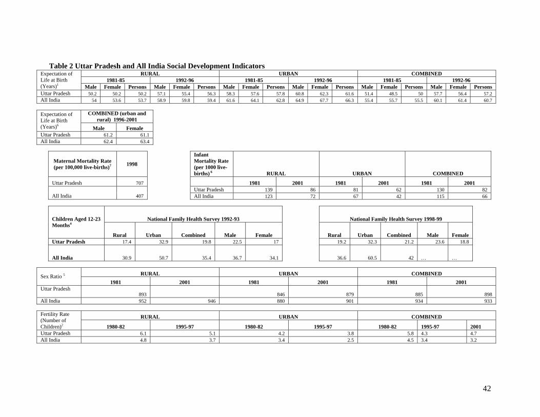
42

Table 2 Uttar Pradesh and All India Social Development Indicators RURAL URBAN COMBINED

1981-85 1992-96 1981-85 1992-96 1981-85 1992-96 Expectation of Life at Birth (Years)1 Male Female Persons Male Female Persons Male Female Persons Male Female Persons Male Female Persons Male Female Persons Uttar Pradesh 50.2 50.2 50.2 57.1 55.4 56.3 58.3 57.6 57.8 60.8 62.3 61.6 51.4 48.5 50 57.7 56.4 57.2 All India 54 53.6 53.7 58.9 59.8 59.4 61.6 64.1 62.8 64.9 67.7 66.3 55.4 55.7 55.5 60.1 61.4 60.7

COMBINED (urban and

rural) 1996-2001 Expectation of Life at Birth (Years)6 Male Female Uttar Pradesh 61.2 61.1 All India 62.4 63.4

Maternal Mortality Rate (per 100,000 live-births)7 1998

Infant Mortality Rate (per 1000 live-births) 6 RURAL URBAN COMBINED

Uttar Pradesh 707 1981 2001 1981 2001 1981 2001 Uttar Pradesh 139 86 81 62 130 82

All India 407

All India 123 72 67 42 115 66

National Family Health Survey 1992-93 National Family Health Survey 1998-99 Children Aged 12-23 Months4

Rural Urban Combined Male Female Rural Urban Combined Male Female Uttar Pradesh 17.4 32.9 19.8 22.5 17 19.2 32.3 21.2 23.6 18.8

All India 30.9 50.7 35.4 36.7 34.1 36.6 60.5 42 … …

RURAL URBAN COMBINED Sex Ratio 5 1981 2001 1981 2001 1981 2001

Uttar Pradesh 893

846 879 885 898

All India 952 946 880 901 934 933

RURAL URBAN COMBINED Fertility Rate (Number of Children)2 1980-82 1995-97 1980-82 1995-97 1980-82 1995-97 2001 Uttar Pradesh 6.1 5.1 4.2 3.8 5.8 4.3 4.7 All India 4.8 3.7 3.4 2.5 4.5 3.4 3.2

43

RURAL URBAN COMBINED 1981 2001 1981 2001 1981 2001 Literacy Rate 3

Male Female Persons Male Female Persons Male Female Persons Male Female Persons Male Female Persons Male Female Persons Uttar Pradesh 43.42 11.7 28.53 68.01 37.74 53.68 64.84 42.73 54.87 78.13 62.05 70.61 47.45 17.19 33.35 70.23 42.97 57.36 All India 49.59 21.7 36.1 71.18 46.58 59.21 … … … 86.42 72.99 80.06 56.38 29.76 43.57 75.64 54.03 65.2

Primary School Completion Rates (percent)8 2004

Uttar Pradesh 50 Notes: 2. Total Fertility Rate has been defined as the number of children a woman would have if hypothetically she lived through her reproductive years (i.e. 15 to 49) experiencing the age specific fertility rates prevailing in the population during a given period 3. Literacy Rate is defined as the proportion of literates to the population in the age group 7+ 3. For Census 1981, Literacy rate was defined for the population 6+. To ensure comparability in this exercise it has been re-estimated for the population 7+ 4. Children are fully vaccinated if they have received BCG, Measles, and 3 doses DPT & Polio Vaccine 5. Overall Sex ratio is defined as females per thousand males for the entire population Sources: 1. Compendium of India's Fertility and Mortality Indicators 1971 to 1997, based on Sample Registration System, RGI 1999 2. Compendium of India’s Fertility and Mortality Indicators, 1971-1997, RGI, New Delhi, 1999 3. 1981 - Census of India-Social and Cultural Tables; 2001 - Based on Preliminary Census 2001 estimates 4. National Family Health Survey I & II 5. Census of India, 1991 & 2001 - Provisional Population Totals, Paper 1, 2001 Statement 19 6. 1981 data: Occasional Paper No.1 of 1997, Table 3, page 112-113, Census of India 2001 data: Sample Registration System Bulletin, Registrar General India, October 2002 7. Sample Registration System Bulletin, Registrar General India, April 2000 8. Attaining the Millennium Development Goals in India: Role of Public Policy & Service Delivery, World Bank 2004

44

Table 3 Percentage of Population Below Poverty Line - Statewise

STATES 1973-74 1983-84 1999-2000

Rural Urban Combined Rural Urban Combined Rural Urban Combined High Income

1. Goa 1.35 7.52 4.402. Gujarat 46.35 52.57 48.15 29.80 39.14 35.78 13.17 15.59 14.073. Haryana 34.23 40.18 35.38 20.56 24.15 21.37 8.27 9.99 8.744. Maharashtra 57.71 43.87 53.24 45.23 40.26 43.44 23.72 26.81 25.025. Punjab 28.21 27.96 28.15 13.20 23.79 16.18 6.35 5.75 6.16

Middle Income 6. Andhra Pradesh 48.41 50.61 48.88 26.53 36.30 28.91 11.05 26.63 15.777. Karnataka 55.14 52.53 54.47 36.33 42.82 38.24 17.38 25.25 20.048. Kerala 59.19 62.74 59.79 39.03 45.68 40.42 9.38 20.27 12.729. Tamil Nadu 57.43 49.40 54.94 53.99 46.96 51.66 20.55 22.11 21.1210. West Bengal 73.16 34.67 63.43 63.05 32.32 54.85 31.85 14.86 27.02

Low Income 11. Bihar 62.99 52.96 61.91 64.37 47.33 62.22 44.30 32.91 42.6012. Madhya Pradesh 62.66 57.66 61.70 46.90 53.06 49.78 37.06 38.44 37.4313. Orissa 67.28 55.62 66.18 67.53 49.15 65.29 48.01 42.83 47.1514. Rajasthan 44.76 52.13 46.14 33.50 37.94 34.46 13.74 19.85 15.2815. Uttar Pradesh 56.53 60.09 57.07 46.45 49.82 47.07 31.22 30.89 31.15

Special Category 16. Arunachal Pradesh 52.67 36.92 51.93 42.60 21.73 40.88 40.04 7.47 33.4717. Assam 52.67 36.92 51.21 42.60 21.73 40.47 40.04 7.47 36.0918. Himachal Pradesh 27.42 13.17 26.39 17.00 9.43 16.40 7.94 4.63 7.6319. Jammu & Kashmir 45.51 21.32 40.83 26.04 17.76 24.24 3.97 1.98 3.4820. Manipur 52.67 36.92 49.96 42.60 21.73 37.02 40.04 7.47 28.5421. Meghalaya 52.67 36.92 50.20 42.60 21.73 36.81 40.04 7.47 33.8722. Mizoram 52.67 36.92 50.32 42.60 21.73 36.00 40.04 7.47 19.4723. Nagaland 52.67 36.92 50.81 42.60 21.73 39.25 40.04 7.47 32.6724. Sikkim 52.67 36.92 50.86 42.60 21.73 39.71 40.04 7.47 36.5525. Tripura 52.67 36.92 51.00 42.60 21.73 40.03 40.04 7.47 34.44All India (States & UTs) 56.44 49.01 54.88 45.65 40.79 44.48 27.09 23.62 26.10Source : Planning Commission in GOI Economic Survey 2001-02, p. 239.

45

Table 4: Percentage distribution of districts ranked on the basis of composite index of Socio-Economics Demographic Indicators

State Total No. of districts 0-100 101-200 201-300 301-400 401-569 All Group-I

1. Andhra Pradesh 23 8.7 47.8 39.1 4.3 0.0 100.0 2. Gujarat 25 8.0 60.0 16.0 12.0 4.0 100.0 3. Haryana 19 21.1 57.9 21.1 0.0 0.0 100.0 4. Karnataka 27 48.1 29.6 18.5 0.0 0.0 100.0 5. Kerala 14 92.9 7.1 0.0 0.0 0.0 100.0 6. Maharashtra 35 17.1 40.0 31.4 11.4 0.0 100.0 7. Punjab 17 70.6 29.4 0.0 0.0 0.0 100.0 8. Tamil Nadu 30 93.3 6.7 0.0 0.0 0.0 100.0 Sub-total (1 to 8) 190 42.1 35.3 17.4 4.7 0.5 100.0

Group-II 9. Assam 20 10.0 5.0 35.0 30.0 20.0 100.0 10. Bihar 55 0.0 0.0 0.0 7.3 92.7 100.0 11. M.P. 61 0.0 6.6 32.8 24.6 36.1 100.0 12. Orissa 30 0.0 6.7 46.7 43.3 3.3 100.0 13. Rajasthan 32 0.0 0.0 0.0 28.1 71.9 100.0 14. Uttar Pradesh 83 0.0 6.0 10.8 27.7 55.4 100.0 15. West Bengal 18 11.1 22.2 33.3 27.8 5.6 100.0 Sub-total (9 to 15) 29 1.3 5.3 18.7 25.1 49.5 100.0 Total 489 17.2 17.0 18.2 17.2 30.5 100.0

Source of basic data: District wise Social Economic Demographic Indicators, National Commission on Population, Government of India 2001. Table 5: Levels of Output and Growth in Punjab, Haryana and Uttar Pradesh during 1962-65, 1970-73, 1980-83 and 1992-95--43 Major Crops (at 1990-93 constant prices)

State Average Value of Output (in Rs million) Percent annual compound growth rate* 1962-65 1970-73 1980-83 1992-95 A B C D

Haryana 16,303.27 23,444.90 31,555.32 54,992.26 4.65 3.02 4.74 4.14 Punjab 22,078.87 36,897.73 58,654.10 92,549.04 6.63 4.74 3.87 4.89

Uttar Pradesh 93,627.51 114,460.68 150,372.86 210,249.47 2.54 2.77 2.83 2.73 All-India 565,642.79 666,706.24 843,474.10 1,260,430.47 2.08 2.38 3.40 2.71

Note:* Percent Annual Compound Growth rate: A) 1970-73 over 1962-65 B) 1980-83 over 1970-73 C) 1992-95 over 1980-83 D) 1992-95 over 1962-65 Source: Bhalla and Singh, 2001 Table 6: State-wise Levels of Growth of Crop Yield during 1962-65, 1970-73, 1980-83 and 1992-95, (at 1990-93 constant prices)

State Average Value of Yield (in Rs million) Percent annual compound growth rate* 1962-65 1970-73 1980-83 1992-95 A B C D

Haryana 3,927.21 5,091.01 6,229.13 10,128.73 3.30 2.04 4.13 3.21 Punjab 5,395.62 7,476.29 9,707.65 13,597.22 4.16 2.65 2.85 3.13 Uttar Pradesh 3,970.10 4,589.98 5,805.13 8,656.20 1.64 1.80 3.15 2.30 All-India 3,738.19 4,256.79 5,090.42 7,388.05 1.64 1.80 3.15 2.30

Note: * Average Yield = (Value output of 43 crop/area under 43 crops) A) 1970-73 over 1962-65 B) 1980-83 over 1970-73 C) 1992-95 over 1980-83 D) 1992-95 over 1962-65 Source: Bhalla and Singh, 2001

46

Table 7: Percent Share of Different Crops in Gross Cropped Area in Punjab, Haryana and U.P. during Trienniums Ending 1962-65, 1970-73, 1980-83 and 1992-95.

State/period Rice Wheat Coarse Cereals Pulses Food-

grains Non-

food grains Nine

Oilseeds Sugarcane Cotton

Haryana

1962-65 4.08 16.71 29.64 35.01 85.44 14.56 5.28 3.12 3.77

1970-73 6.16 25.88 28.49 24.71 85.24 14.76 3.90 2.93 5.02

1980-83 9.65 31.35 22.56 16.24 79.80 20.20 4.61 2.69 6.85

1992-95 13.15 36.16 14.18 8.34 71.83 28.17 12.44 2.55 10.06

Punjab

1962-65 6.43 37.52 13.86 20.5 78.31 21.69 5.26 2.82 11.97

1970-73 8.88 47.54 15.68 7.96 80.07 19.93 6.52 2.25 9.31

1980-83 20.78 48.42 7.9 4.78 81.88 18.12 3.57 1.55 11.34

1992-95 31.25 48.71 3.59 1.51 85.07 14.93 2.83 1.47 9.53

Uttar Pradesh

1962-65 18.48 16.85 22.63 19.65 77.61 22.39 15.29 5.48 0.34

1970-73 18.26 24.18 21.17 14.38 77.99 22.01 15.24 5.25 0.21

1980-83 20.26 31.12 15.32 11.43 78.12 21.88 13.98 6.17 0.14

1992-95 22.35 36.53 12.45 11.92 83.26 16.74 7.14 7.63 0.05

All-India

1962-65 23.78 8.92 29.2 15.93 77.85 22.15 10.59 1.56 5.36

1970-73 23.84 12.1 28.04 13.96 77.94 22.06 10.58 1.59 4.91

1980-83 23.96 13.68 25.08 13.91 76.63 23.37 10.92 1.85 4.78

1992-95 24.91 14.32 19.81 13.17 72.21 27.79 15.31 2.13 4.42 Note: Remaining percent shares are attributed to other crops. Source: Bhalla and Singh, 2001.

47

Table 8: Uttar Pradesh and Top Producing States of Major Crops; 1972-73, 1984-85 and 2001-02 Wheat

1972-73 1984-85 2001-02

Area Yield Production Area Yield Production Area Yield Production

('000 ha) (kg/ha) ('000 tons) % of all-

India production

('000 ha) (kg/ha) ('000 tons) % of all-

India production

('000 ha) (kg/ha) ('000 tons) % of all-

India production

Uttar Pradesh 5,715.8 1,229.0 7,024.9 28.4 8,003.1 1,897.0 15,179.1 34.4 9,089.0 2,760.0 25,018.5 34.8

Punjab 2,404.3 2,233.0 5,368.0 21.7 3,094.0 3,289.0 10,176.0 23.1 3,420.0 4,530.0 15,499.0 21.6

Haryana 1,270.0 1,757.0 2,231.0 9.0 1,704.7 2,593.0 4,421.0 10.0 2,300.0 4,100.0 9,437.0 13.1 Rice

1972-73 1984-85 2001-02

Area Yield Production Area Yield Production Area Yield Production

('000 ha) (kg/ha) ('000 tons) % of all-

India production

('000 ha) (kg/ha) ('000 tons) % of all-

India production

('000 ha) (kg/ha) ('000 tons) % of all-

India production

West Bengal 5,069.4 1,127.0 5,715.3 14.6 5,204.5 1,555.0 8,092.5 13.9 6,069.1 2,510.0 15,256.7 16.4 Uttar Pradesh 4,147.7 712.0 2,953.7 7.5 5,225.2 1,275.0 6,662.6 11.4 5,876.8 2,120.0 12,458.5 13.4

Punjab 475.5 2,008.0 955.0 2.4 1,644.0 3,074.0 5,054.0 8.7 2,487.0 3,540.0 8,816.0 9.5

Haryana* 291.0 1,588.0 462.0 1.2 557.3 2,446.0 1,363.0 2.3 1,027.0 2,650.0 2,724.0 2.9 Sugarcane

1972-73 1984-85 2001-02

Area Yield Production Area Yield Production Area Yield Production

('000 ha) (kg/ha) ('000 tons) % of all-

India production

('000 ha) (kg/ha) ('000 tons) % of all-

India production

('000 ha) (kg/ha) ('000 tons) % of all-

India production

Uttar Pradesh 1,270.5 43,433.0 55,169.3 44.2 1,504.8 45,884.0 69,046.9 40.5 2,035.0 57,110.0 116,218.5 38.6 Maharashtra 146.0 81,628.0 11,917.7 9.5 254.4 79,312.0 28,108.0 16.5 578.0 78,100.0 45,140.0 15.0

Tamil Nadu 144.0 84,118.0 12,113.0 9.7 169.5 95,236.0 16,139.4 9.5 326.1 111,430.0 36,335.7 12.1

48

Table 8 continued… Oilseeds

1972-73 1984-85 2001-02

Area Yield Production Area Yield Production Area Yield Production

('000 ha) (kg/ha) ('000 tons) % of all-

India production

('000 ha) (kg/ha) ('000 tons) % of all-

India production

('000 ha) (kg/ha) ('000 tons) % of all-

India production

Kerala 773.2 5,096.9 3,940.9 30.0 714.2 4,817.1 3,440.4 17.3 945.1 5,821.3 5,501.7 17.7 Tamil Nadu 1,389.7 1,544.8 2,146.8 16.3 1,237.2 2,085.9 2,580.7 13.0 1,378.7 3,439.8 4,742.4 15.3

Uttar Pradesh* 689.7 650.3 448.5 3.4 872.9 620.1 541.3 2.7 1,293.3 835.8 1,080.9 3.5 Vegetables, Roots & Tubers

1972-73 1984-85 2001-02

Area Yield Production Area Yield Production Area Yield Production

('000 ha) (kg/ha) ('000 tons) % of all-

India production

('000 ha) (kg/ha) ('000 tons) % of all-

India production

('000 ha) (kg/ha) ('000 tons) % of all-

India production

West Bengal 1,075.0 16,539.0 17,779.4 18.9 Uttar Pradesh 668.1 19,504.0 13,030.4 13.9

Bihar 707.8 14,439.0 10,219.7 10.9 Pulses

1972-73 1984-85 2001-02

Area Yield Production Area Yield Production Area Yield Production

('000 ha) (kg/ha) ('000 tons) % of all-

India production

('000 ha) (kg/ha) ('000 tons) % of all-

India production

('000 ha) (kg/ha) ('000 tons) % of all-

India production

Uttar Pradesh 505.3 1,469.2 742.4 13.8 2,006.5 1,123.3 2,254.0 30.5 1,857.9 796.2 1,479.3 20.7 Maharashtra 1,584.6 258.9 410.2 7.6 2,324.1 392.7 912.6 12.3 2,876.6 446.6 1,284.6 18.0

Andhra Pradesh 1,274.6 220.4 280.9 5.2 1,293.1 374.6 484.4 6.5 1,639.7 461.0 755.9 10.6 Note: *State is not among the top three producers of rice, but is included for comparison Data for U.P. varies from the data presented in Table 21, which is from a different source. Source: CMIE Agriculture, 2004.

49

Table 9: State-wise Level of Inputs used during 1962-65, 1980-83 and 1992-95 State Number of Tractors1 Number of pumpsets Consumption of fertilizers

(per 1000 ha of net sown area) (per 1000 ha of NSA) (kg/ha) 1962-65 1980-83 1987 1999-00 1962-65 1980-83* 1962-65 1980-83 1992-95 Haryana 0.7 17.07 55.5 93 2.32 71.5 2.53 68.99 191.19Punjab 2.41 25.35 81.78 102 8.2 157.69 7.84 192.07 296.68U.P. 0.5 8.25 20.88 39.5 1.45 63.93 4.06 75.36 134.27All-India 0.3 3.68 11.73 20.84 4.58 49.16 4.33 42.62 89.08

State % of GCA irrigated Cropping intensity2 (GCA/NSA)

1962-65 1980-83 1992-95 1962-65 1980-83 1992-95 1997-2000

Haryana 31.1 62.21 77.14 1.31 1.53 1.65 1.71Punjab 58.42 86.64 94.58 1.29 1.64 1.81 1.87U.P. 26.99 47.42 62.29 1.28 1.43 1.48 1.47All-India 19 29.29 35.66 1.15 1.24 1.3 1.3

1Data through 1987 is from Bhalla and Singh (2001). 1999-2000 data is from CMIE (2004). 2Data through 1995 is from Bhalla and Singh (2001). Later data is from CMIE (2004). *For later years, see table 10 below. NSA = net sown area Source: Bhalla and Singh (2001); CMIE (2004)

50

Table 10 State-wise Disaggregation of Electric and Diesel Pumpsets (per 1000 hectares of net sown area)

1986-87 1991-92 2001

State Electric Pumpsets

Diesel Pumpsets

Total Pumpsets

Electric Pumpsets

Diesel Pumpsets

Total Pumpsets

Electric Pumpsets

Haryana 66.12 63.28 129.40 89.08 54.50 143.59 120.00 Punjab 51.72 107.67 159.39 116.49 52.91 169.40 191.50 U.P. 18.16 77.19 95.36 22.01 109.87 131.88 50.00

Note: State-wise data for years later than 1992 that included diesel pumpsets was not obtainable. Later data, as shown here, consisted only of information on electric pumpsets. However, later disaggregated data for U.P. was available and is presented in Table 15. Source: Data through 1992 from CMIE (2004). 2001 data from Central Electricity Authority (2000-01).

51

Table 11: Indicators of Development in the Eastern and Western Alluviums of U.P. General Western Eastern U.P. Population in million (2001) 61 66.6 166 Geographical area sq km (2001) 89589a 87294a 240,928 Percent of urban population to total population (1991) 26.3 11.6 20.78* Population density (2001) 782 860 689 Percent of literacy (2001) 59.5 53.8 57.36 Sex ratio (2001) 862 978 898 Percent of SC to total population (1991) 18.6 20.7 21 Average monsoon rainfall (mm) (2002) 765.7 891.3 N.A.. Infrastructure Per capita electricity consumption (kwh 1998-99) 206.8 169.2 184.9 Percent of electrified villages (3/31/2000) 88.8 77 79 Telephones per lakh population (1999-2000) 1520 778 1248 Length of metalled road under PWD per 1,000 sq km (1999-2000) 1520 778 1246 Consumption of electricity in Ag as percent of total cons. (1998-99) 43.4 25 31 Credit Facilities Credit deposit ratio (June 1999-2000) 22.5 22 21.6 Scheduled commercial banks per lakh pop (1999-2000) 5.2 5.3 5.3 Cooperative agricultural marketing centers per lakh pop (1999-00) 3.1 1.8 2.2 Cooperative marketing societies per lakh pop (1999-2000) 0.17 0.11 0.16 Joint agricultural cooperative societies (1999-2000) 1 0.6 0.8 Agriculture-related Percent of marginal holdings (<1 ha, 1995-96) 66.8 83 75.4 Percent of area under marginal holdings (1995-96) 28.1 44.8 33.7 Average size of marginal holding (ha 1995-96) 0.42 0.35 0.39 Percent of small holdings (1-2 ha) (1995-96) 17.8 10.9 14.6 Percent of area under small holdings (1995-96) 24.9 22.8 23.8 Percent of farmers vs. main workers (1990-91) 47.9 54.8 53.3 Percent of agricultural laborers vs. main workers (1990-91) 18.5 22.5 18.9 Cultivable area as percent of reported area (1994-95) 82.7 77 70.9 Net cultivated area as percent of cultivable area (1998-99) 90.8 86.1 83.4 Net irrigated area as percent of net cropped area (1998-99) 89.7 61.4 72.2 Percent of area irrigated by state tubewells (2001-02) 2.4 5.6 305 Percent of area irrigated by private tubewells (1998-99) 77 65 68 Cropping intensity (1998-99) 156 150.8 148.8 Commercial crop area as percent of gross cropped area (1998-99) 32.1 10.4 20.5 Distribution of fertilizer per ha gross cropped area (in ha 1998-99) 148.1 116.2 118.2 Availability of tractor per gross cropped area (in ha 1998-99) 32.1 74.4 47.1 Value of agricultural produce per ha on current prices (1997-98) 21280 15677 17857 Productivity of foodgrains (kg/ha 1998-99) 2410 1920 1740 Productivity of wheat (kg/ha 2001-02) 3236 2377 2755 Productivity of rice (kg/ha 2001-02) 2203 2125 2117 Productivity of potatoes (kg/ha 1998-99) 25030 20050 22802 Productivity of oil seeds (kg/ha 1998-99) 890 550 700 Productivity of sugarcane (kg/ha 2001-02) 58094 48591 57980 Productivity of pulses (kg/ha 2001-02) 810 869 886 Percent of kharif area affected by floods (1999-2000) 0.92 8.5 3.9 Gross value of agricultural produce per rural person on current prices (1997-98) 3447 2435 3594 Income from primary sector as percent of net domestic output (1997-98) 38.6 36.3 36.9 * 2001 data a) Land area data does not include the districts of Kannauj and Auraiya in western U.P. and Kaushambi, Ambedaker Nagar and Basti in eastern U.P. Since some districts were divided, it is likely that the districts are accounted for in land area but were measured under a different name. Source: Pant (2004); Census of India: Uttar Pradesh (2001); State Government of U.P. (2004)

52

Table 13: Net Irrigated Area as Percentage of Net Cropped Area in Uttar Pradesh, by region, 1960-1961 through 1985-1986 Region 1960-61 1964-65 1970-71 1975-76 1980-81 1985-86 1998-99 Western U.P. 34.3 38.7 56.2 65.3 72.4 77.4 89.7 Eastern U.P. 35.5 36.3 40.8 44.0 52.7 56.2 61.4 Source: Sharma and Poleman (1993) for data through 1986. Later data from Pant (2003).

Table 12: Fertilizer Consumption Per Hectare of Gross Cropped Area in Uttar Pradesh, by region, 1965-1966 through 1985-1986 (kg/ha) Region 1965-66 1970-71 1975-76 1980-81 1985-86 1998-99 Western U.P. 6.0 22.7 27.0 58.5 94.6 148.1 Eastern U.P. 4.2 19.6 22.6 49.6 82.9 116.2 Source: Sharma and Poleman (1993) for data through 1986. Later data from Pant (2004).

53

Table 14: Tubewell Irrigated Area in Uttar Pradesh as Percentage of Net Irrigated Area (NIA), and as Percentage of Net Cropped Area (NCA) by region, 1960-1961 through 1998-99

1960-61 1964-65 1970-71 1975-76 1980-81 1985-86 1998-99 Region NIA NCA NIA NCA NIA NCA NIA NCA NIA NCA NIA NCA NIA

Western U.P. 17.6 6.1 20.1 7.8 40.9 23.0 52.0 34.0 59.0 42.7 64.6 50.0 79.4 Eastern U.P. 8.3 2.9 10.8 3.9 31.9 13.1 42.0 18.4 59.1 31.2 61.0 34.3 69.6 Source: Sharma and Poleman (1993) for data through 1986. Later data from Pant (2003). Table 15: Diesel and Electric Tubewells in Eastern and Western U.P., 1979-80 to 1998-99 Year Diesel Pumping Set Electric Tubewells Total Diesel and Electric East West U.P. East West U.P. East West U.P. 1979-80 128954 317028 581998 183083 217432 465969 312037 534460 1047967 1984-85 258727 526343 1030488 285902 290068 674753 544629 816411 1705241 1993-94 525389 710862 1624923 81431 194027 306978 606820 904889 1931901 1998-99 1138065 1149837 2965357 183623 325743 570748 1321688 1475580 3536105

Year Proportion of electric tubewells to

total tubewells

Proportion of tubewells located

in eastern U.P. East West U.P. Year 1979-80 58.67 40.68 44.46 1979-80 29.78 1984-85 52.49 53.26 39.57 1984-85 31.94 1993-94 13.42 21.44 15.89 1993-94 31.41 1998-99 13.89 22.08 16.14 1998-99 37.38 Source: Pant (2004). Proportions calculated by authors using Pant's data.

54

Table 16: Cropping Intensity in Uttar Pradesh by region, 1960-1961 through 1985-1986 (percentage)

Region 1960-61 1964-65 1970-71 1975-76 1980-81

1985-86

1998-99

Western U.P. 127.1 129.3 139.4 141.5 150.7 154.2 156 Eastern U.P. 131.7 132.8 134.0 134.0 145.2 150.0 150.8 Source: Sharma and Poleman (1993) for data through 1986. Later data from Pant (2003).

Table 17: Yields of Wheat and Rice in Uttar Pradesh, by region, 1964-1965 through 2001-02

(Kg/ha) Western U.P. Eastern U.P.

Year Wheat Rice Wheat Rice

1964-65 907 635

726

635

1970-71 1,270

817

998

635

1975-76 1,179

907

998

726

1980-81 1,633

1,088

1,179

726

1985-86 2,268

1,632

1,633 1270

1995-96 2,898 2,330

2,178 1642

2001-02 3236 2203 2377 2125 Source: Sharma and Poleman (1993) for data through 1986. Later data from Government of U.P. (2004).

55

Table 18 Percentage Area of Major Crops in Gross Cropped Area in

Uttar Pradesh, by region, 1960-61 through 1985-86 Western Uttar Pradesh Crop 1960-61 1964-65 1970-71 1975-76 1980-81 1985-86 Wheat 22.3 21.6 31.6 31.1 34 33 Rice 10.1 10.5 10.5 11.1 12.4 17.3 Coarse cereals 26 24.9 23.1 23.4 19.4 17.3 Pulses 18.5 18 11.5 9.3 7.4 7.9 Total foodgrains 76.9 75 76.7 74.8 73.1 70.7 Oilseeds 5 5 3.4 4.5 3.9 4.7 Sugarcane 10.4 10.3 9.3 10.9 9.8 10.3 Potato 0.6 0.6 0.8 1 1.4 1.5 Vegetables and fruits N.A. 1 1 1.5 2 2.7 Others 7.1 8.1 8.8 7.3 9.8 10.1 Eastern Uttar Pradesh Crop 1960-61 1964-65 1970-71 1975-76 1980-81 1985-86 Wheat 11.7 12.9 18.2 22.2 31.7 33.1 Rice 31.1 32.1 31.4 32.4 34.6 35 Coarse cereals 28.7 27.5 29.6 21 16.5 10 Pulses 16.5 15 11.2 13.5 11.2 11.1 Total foodgrains 88 87.5 90.4 89.1 91.1 89.7 Oilseeds 5 4.5 1.5 1.4 1.5 1.5 Sugarcane 4.4 4.2 4.2 4.6 3.3 3.3 Potato 0.5 0.5 0.8 0.9 1.1 1.1 Vegetables and fruits N.A. 0.6 0.6 0.8 1 3.1 Others 2.1 2.7 2.5 3.2 3 1.1 Source: Sharma and Poleman (1993).

56

Table 19: Net and Gross Irrigated Area (in '000 ha) by District in Eastern and Western U.P., 2001-02 Western U.P. Gross Irrigated Area Net Irrigated Area District SAHARANPUR 374 249 MUZAFFARNAGAR 483 324 MEERUT 312 192 BAGPAT 175 110 GHAZIABAD 227 140 G.BUDDHA NGR. 161 121 ALIGARH 415 294 HATHARAS 189 145 MATHURA 324 266 AGRA 251 236 FIROZABAD 208 177 MAINPURI 282 190 ETAH 438 312 BAREILLY 481 267 BUDAUN 503 387 SHAHJAHANPUR 552 357 PILIBHIT 345 214 BIJNOR 379 285 MORADABAD 472 251 J.B.FULE NAGAR 223 165 RAMPUR 339 188 FARRUKHABAD 168 131 KANNAUJ 167 129 ETAWAH 172 118 AURAIYA 173 109 Western U.P. 7813 5357

57

Table 19 Net and Gross Irrigated Area by District in E and W U.P., 2001-02 cont. Eastern U.P. Gross Irrigated Area Net Irrigated Area District ALLAHABAD 392 244 KAUSHAMBI 113 85 PRATAPGARH 284 195 VARANASI 130 99 CHANDAULI 202 129 GHAZIPUR 227 140 JAUNPUR 350 258 MIRZPUR 300 134 SONBHADRA 79 54 S. RAVI DAS NGR 75 57 AZAMGARH 385 267 MAU 152 114 BALLIA 236 177 GORAKHPUR 229 205 MHARAJGANJ 172 152 DEORIA 182 156 KUSHI NAGAR 242 171 BASTI 170 130 SIDDHARTH NAGAR 147 144 SANT KABIR NGR 105 103 FAIZABAD 237 148 AMBEDKAR NAGAR 271 155 SULTANPUR 309 213 GONDA 207 184 BALRAMPUR 99 82 BAHRAICH 155 142 SHRAVASTI 59 54 Eastern U.P. 5509 3992 UTTAR PRADESH 18220 12828 Source: CMIE (2004)

Table 20: Region-wise Irrigation Sources as a Proportion of Net Irrigated Area, 2001-02

Region Canal Government Tubewell

Private Tubewell

Total Tubewell

Other wells Tank

Other Means

Western U.P. 14.10 2.38 77.09 79.47 5.94 0.06 0.43 Eastern U.P. 24.27 5.55 65.85 71.40 2.84 1.07 0.42 U.P. 21.19 3.50 67.89 71.39 5.82 0.66 0.94 Source: Government of U.P. (2004)

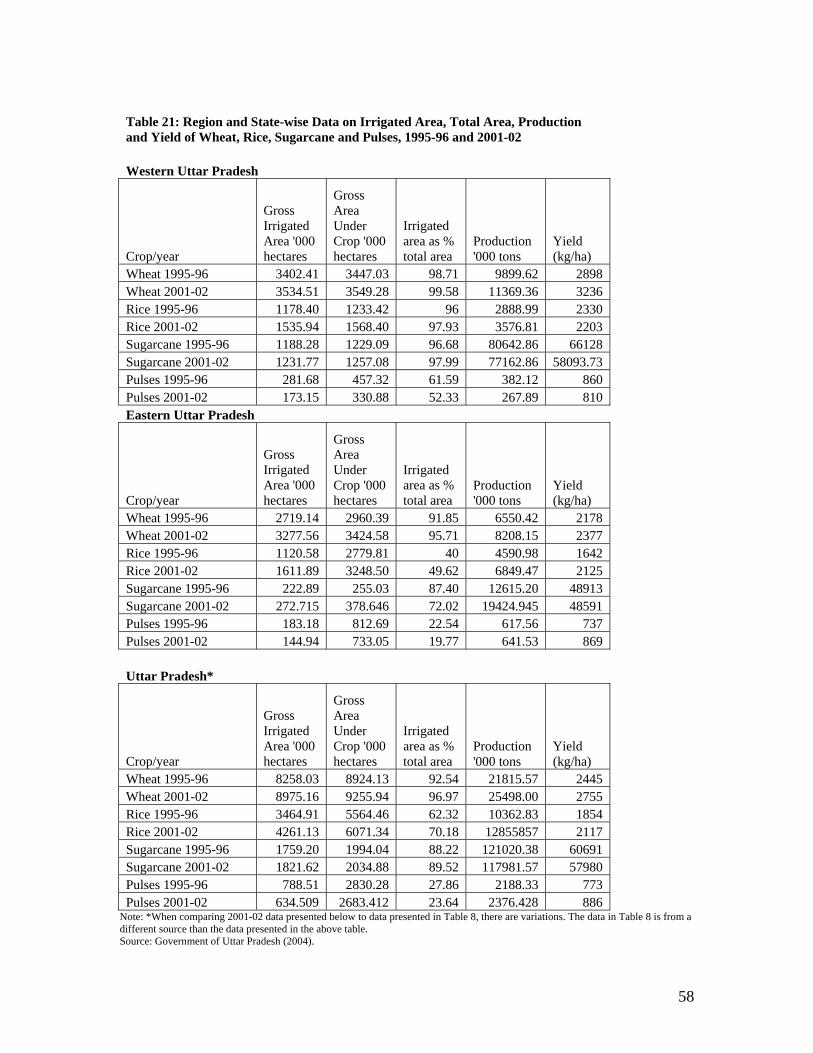
58

Table 21: Region and State-wise Data on Irrigated Area, Total Area, Production and Yield of Wheat, Rice, Sugarcane and Pulses, 1995-96 and 2001-02 Western Uttar Pradesh

Crop/year

Gross Irrigated Area '000 hectares

Gross Area Under Crop '000 hectares

Irrigated area as % total area

Production '000 tons

Yield (kg/ha)

Wheat 1995-96 3402.41 3447.03 98.71 9899.62 2898 Wheat 2001-02 3534.51 3549.28 99.58 11369.36 3236 Rice 1995-96 1178.40 1233.42 96 2888.99 2330 Rice 2001-02 1535.94 1568.40 97.93 3576.81 2203 Sugarcane 1995-96 1188.28 1229.09 96.68 80642.86 66128 Sugarcane 2001-02 1231.77 1257.08 97.99 77162.86 58093.73 Pulses 1995-96 281.68 457.32 61.59 382.12 860 Pulses 2001-02 173.15 330.88 52.33 267.89 810 Eastern Uttar Pradesh

Crop/year

Gross Irrigated Area '000 hectares

Gross Area Under Crop '000 hectares

Irrigated area as % total area

Production '000 tons

Yield (kg/ha)

Wheat 1995-96 2719.14 2960.39 91.85 6550.42 2178 Wheat 2001-02 3277.56 3424.58 95.71 8208.15 2377 Rice 1995-96 1120.58 2779.81 40 4590.98 1642 Rice 2001-02 1611.89 3248.50 49.62 6849.47 2125 Sugarcane 1995-96 222.89 255.03 87.40 12615.20 48913 Sugarcane 2001-02 272.715 378.646 72.02 19424.945 48591 Pulses 1995-96 183.18 812.69 22.54 617.56 737 Pulses 2001-02 144.94 733.05 19.77 641.53 869 Uttar Pradesh*

Crop/year

Gross Irrigated Area '000 hectares

Gross Area Under Crop '000 hectares

Irrigated area as % total area

Production '000 tons

Yield (kg/ha)

Wheat 1995-96 8258.03 8924.13 92.54 21815.57 2445 Wheat 2001-02 8975.16 9255.94 96.97 25498.00 2755 Rice 1995-96 3464.91 5564.46 62.32 10362.83 1854 Rice 2001-02 4261.13 6071.34 70.18 12855857 2117 Sugarcane 1995-96 1759.20 1994.04 88.22 121020.38 60691 Sugarcane 2001-02 1821.62 2034.88 89.52 117981.57 57980 Pulses 1995-96 788.51 2830.28 27.86 2188.33 773 Pulses 2001-02 634.509 2683.412 23.64 2376.428 886

Note: *When comparing 2001-02 data presented below to data presented in Table 8, there are variations. The data in Table 8 is from a different source than the data presented in the above table. Source: Government of Uttar Pradesh (2004).