agricultural exports from latin america and the caribbean ... · 4.1 challenges of sustainable food...

WORLD BANK

Agricultural Exports from Latin America and the

Caribbean: Harnessing Trade to Feed the World and Promote Development

Nabil Chaherli and John Nash

Pub

lic D

iscl

osur

e A

utho

rized

Pub

lic D

iscl

osur

e A

utho

rized

Pub

lic D

iscl

osur

e A

utho

rized

Pub

lic D

iscl

osur

e A

utho

rized

i

Contents

CONTENTS .............................................................................................................................................................. I

FIGURES ............................................................................................................................................................................ II

TABLES .................................................................................................................................................................. V

BOXES ................................................................................................................................................................... V

ACKNOWLEDGMENTS .......................................................................................................................................... VI

CHAPTER 1. INTRODUCTION AND SUMMARY .................................................................................................. 1

1.1 LATIN AMERICA AND THE CARIBBEAN’S RECENT PERFORMANCE IN AGRICULTURAL MARKETS: OVERALL GOOD NEWS ......................... 2

1.2 THE ENABLING ENVIRONMENT FOR AGRICULTURAL TRADE: POTENTIAL CONSTRAINTS AND WHAT CAN BE DONE TO OVERCOME THEM .. 6

1.2.1 Trade policy .......................................................................................................................................................... 6

1.2.2 Infrastructure and logistics ................................................................................................................................ 11

1.3 THE FUTURE: HOW CAN LAC HELP FEED THE WORLD? ....................................................................................................... 18

1.3.1 Removing the constraints: priorities for the future of Latin America and the Caribbean’s sustainable

agricultural trade ........................................................................................................................................................ 19

CHAPTER 2. LATIN AMERICA AND THE CARIBBEAN’S RECENT PERFORMANCE IN AGRICULTURAL TRADE ...... 21

2.1 AGRICULTURAL PRODUCTION AND CONSUMPTION PATTERNS .............................................................................................. 21

2.2 WORLD AND LATIN AMERICA AND THE CARIBBEAN TRADE: TRENDS AND CHANGES .................................................................. 24

2.2.1 World merchandise trade: general patterns ...................................................................................................... 24

2.2.2 Structure of trade in Latin America and the Caribbean ..................................................................................... 24

2.2.3 The anatomy of Latin America and the Caribbean’s agriculture export growth ................................................ 29

2.2.4 Sector composition of Latin America and the Caribbean’s agricultural trade ................................................... 31

2.2.5 Origins of Latin America and the Caribbean’s agricultural exports ................................................................... 34

2.2.6 Destination markets ........................................................................................................................................... 35

2.3 DIVERSIFICATION AND MOVING UP THE QUALITY LADDER .................................................................................................... 37

2.3.1 Changes in export concentration: Is Latin America and the Caribbean’s agricultural trade becoming more

diversified? .................................................................................................................................................................. 37

2.3.2 Value adding and moving up the value chain .................................................................................................... 43

2.4 WHAT HAS BEEN DRIVING THE DYNAMOS? ...................................................................................................................... 48

2.4.1 Argentina ........................................................................................................................................................... 48

2.4.2 Brazil .................................................................................................................................................................. 52

CHAPTER 3. THE ENABLING ENVIRONMENT FOR AGRICULTURAL TRADE: POTENTIAL CONSTRAINTS AND

WHAT CAN BE DONE TO OVERCOME THEM ........................................................................................................ 58

3.1 EXTERNAL ENVIRONMENT: BARRIERS TO EXPORTS FROM LATIN AMERICA AND THE CARIBBEAN COUNTRIES .................................. 58

3.2 TRADE POLICIES OF LATIN AMERICA AND THE CARIBBEAN COUNTRIES ................................................................................... 61

3.3 TRADE AGREEMENTS: THE LATIN SPAGHETTI BOWL ............................................................................................................ 63

3.4 LOGISTICS AND TRADE FACILITATION ............................................................................................................................... 67

3.4.1 How important is trade facilitation? .................................................................................................................. 68

3.4.2 Agricultural trade logistics in Latin America and the Caribbean: benchmarking and breaking it down ............ 75

3.4.3 Drilling down: What are the most important logistics and trade facilitation challenges at the subregional and

country levels? ............................................................................................................................................................ 82

3.5 CONCLUSIONS AND POLICY IMPLICATIONS ........................................................................................................................ 99

3.5.1 Global trade policy ............................................................................................................................................. 99

ii

3.5.2 For Latin America and the Caribbean ................................................................................................................. 99

3.5.3 Policy recommendations for logistics and trade facilitation ............................................................................ 101

CHAPTER 4. ASSESSING LATIN AMERICA AND THE CARIBBEAN’S CONTRIBUTION TO GLOBAL FOOD AND FEED

SECURITY IN 2050 ...............................................................................................................................................104

4.1 CHALLENGES OF SUSTAINABLE FOOD SECURITY TOWARD 2050 .......................................................................................... 104

4.2 DEMAND DYNAMICS AND SUPPLY-SIDE CONSTRAINTS ...................................................................................................... 105

4.2.1 Demand dynamics ............................................................................................................................................ 105

4.2.2 Supply-side constraints..................................................................................................................................... 107

4.3 METHODOLOGY USED FOR THE ANALYSIS ...................................................................................................................... 109

4.4 AGRICULTURAL EXPORTS OUTLOOK TO 2050: THE CURRENT-PATH CASE .............................................................................. 110

4.5 EMERGING MARKET GROWTH AND THE RESHAPING OF THE GLOBAL FOOD ECONOMY ............................................................. 115

4.6 FOOD SECURITY, TRADE, AND CLIMATE CHANGE .............................................................................................................. 117

4.7 THE GLOBAL GRID, LATIN AMERICA AND THE CARIBBEAN’S BUSINESS ENVIRONMENT, AND THE FOOD CONNECTION ..................... 121

4.8 GREEN GROWTH AND AGRICULTURAL EXPORTS IN LATIN AMERICA AND THE CARIBBEAN ......................................................... 124

4.9 SUMMARY AND CONCLUSIONS .................................................................................................................................... 129

REFERENCES .......................................................................................................................................................132

Figures

FIGURE 1.1. SHARES (LEFT AXIS) AND CONTRIBUTION TO GROWTH BY ORIGIN OF LATIN AMERICA AND THE CARIBBEAN’S AGRICULTURAL

EXPORTERS, 1995 AND 2009 (PERCENT)................................................................................................................................ 3

FIGURE 1.2. SHARES (LEFT AXIS) AND CONTRIBUTION TO GROWTH BY EXPORT DESTINATION, 1995 AND 2009 (PERCENT) ..................... 4

FIGURE 1.3. TOP 10 LATIN AMERICA AND THE CARIBBEAN AGRICULTURAL EXPORTS TO DEVELOPED AND DEVELOPING ECONOMIES, 2009 4

FIGURE 1.4 ARGENTINE GRAIN PRODUCTION, 1979–2010 (MILLIONS OF TONS) ........................................................................... 5

FIGURE 1.5. MARKET ACCESS OVERALL TRADE RESTRICTIVENESS INDICES FOR AGRICULTURAL EXPORTS BY REGION, 2009 (PERCENT) ...... 7

FIGURE 1.6. RELATIVE RATES OF ASSISTANCE BY REGION, 1965–2009 ........................................................................................ 8

FIGURE 1.7. REAL EFFECTIVE EXCHANGE RATES, 1980–2010 (2005 = 100) ................................................................................ 9

FIGURE 1.8. INCREASE IN EXPORTS FROM AN IMPROVEMENT IN SOFT INFRASTRUCTURE TO THE LEVELS OF ORGANIZATION FOR ECONOMIC

CO-OPERATION AND DEVELOPMENT COUNTRIES .................................................................................................................... 12

FIGURE 1.9. LOGISTICS COST AS A PERCENTAGE OF FOOD PRODUCT VALUE, 2004 (PERCENT).......................................................... 13

FIGURE 1.10. TRADE FACILITATION: COMPARING LATIN AMERICA AND THE CARIBBEAN WITH OTHER REGIONS ................................... 14

FIGURE 1.11. COST TO EXPORT AND IMPORT—GLOBAL COMPARISON, 2011 ($ PER CONTAINER) ................................................... 15

FIGURE 1.12. PINEAPPLE SUPPLY CHAIN FROM COSTA RICA TO ST. LUCIA ................................................................................... 16

FIGURE 2.1 AGRICULTURAL NET PRODUCTION VALUE INDEX: LATIN AMERICA AND THE CARIBBEAN AND THE WORLD, 1980–2009 (1980

= 100) .......................................................................................................................................................................... 22

FIGURE 2.2. SHARE OF WORLD NET PRODUCTION VALUE IN 2004–06 INTERNATIONAL DOLLARS, 1980–2009 (PERCENT) .................. 22

FIGURE 2.3. EVOLUTION OF WORLD TRADE COMPOSITION, 1990–2009 (US$ MILLIONS) ............................................................. 24

FIGURE 2.4. LATIN AMERICA AND THE CARIBBEAN’S SHARE OF WORLD TRADE BY GROUP, 2009 (PERCENT) ...................................... 25

FIGURE 2.5. MERCHANDISE TRADE AS A SHARE OF GDP, (PERCENT) .......................................................................................... 25

FIGURE 2.6. LAC’S EXPORT STRUCTURE ($ BILLIONS) .............................................................................................................. 26

FIGURE 2.7. LATIN AMERICA AND THE CARIBBEAN’S IMPORT STRUCTURE (PERCENT) ..................................................................... 27

FIGURE 2.8. LAC’S INTRAREGIONAL TRADE STRUCTURE 2001, 2008, 2009 (US$ BILLIONS) ......................................................... 27

FIGURE 2.9. SHARE OF LATIN AMERICA AND THE CARIBBEAN INTRATRADE IN TOTAL TRADE BY GROUP (PERCENT) ............................... 28

FIGURE 2.10. ANNUAL GROWTH RATES OF LATIN AMERICA AND THE CARIBBEAN’S EXPORTS (PERCENT) ........................................... 28

FIGURE 2.11. SELECTED INDICATORS ON THE COMPOSITION OF TRADE, 2009 (PERCENT) ............................................................... 29

iii

FIGURE 2.12. VALUE OF LATIN AMERICA AND THE CARIBBEAN’S AGRICULTURAL EXPORTS, 1995–2009 .......................................... 30

(US$ BILLIONS) ............................................................................................................................................................... 30

FIGURE 2.13. LATIN AMERICA AND THE CARIBBEAN’S SHARE IN WORLD AGRICULTURAL EXPORTS (PERCENT) ..................................... 30

FIGURE 2.14. AGRICULTURAL AND FOOD MERCHANDISE TRADE AS SHARE OF AGRICULTURAL GDP (PERCENT) .................................... 31

FIGURE 2.15. LATIN AMERICA AND THE CARIBBEAN’S SHARE OF WORLD AGRICULTURAL EXPORTS .................................................... 31

FIGURE 2.16. SHARES OF GROWTH (LEFT AXIS) AND CONTRIBUTION TO GROWTH (RIGHT AXIS) BY PRODUCT GROUP (PERCENT) ............ 32

FIGURE 2.17. CONTRIBUTIONS TO EXPORT GROWTH BY PRODUCT CATEGORY AND SUBREGION, 1995–2009 (PERCENT) ..................... 33

FIGURE 2.18. SHARE OF TOP 10 PRODUCT GROUPS IN TOTAL AGRICULTURAL EXPORTS, 2001 AND 2009 (PERCENT) .......................... 34

FIGURE 2.19. SHARES OF GROWTH (LEFT AXIS) AND CONTRIBUTION TO GROWTH (RIGHT AXIS) BY ORIGIN OF LATIN AMERICA AND THE

CARIBBEAN’S AGRICULTURAL EXPORTS, 1995 AND 2009 (PERCENT) .......................................................................................... 35

FIGURE 2.20. SHARES AND CONTRIBUTION TO GROWTH ACCORDING TO EXPORT DESTINATION ........................................................ 36

FIGURE 2.21. TOP 10 LATIN AMERICA AND THE CARIBBEAN AGRICULTURAL EXPORTS TO DEVELOPED AND DEVELOPING ECONOMIES, 2009

.................................................................................................................................................................................... 36

FIGURE 2.22. LATIN AMERICAN AND THE CARIBBEAN’S EXPORT PRODUCT DIVERSIFICATION, 1995–2009 (HERFINDAHL-HIRSCHMAN

INDEX) ........................................................................................................................................................................... 38

FIGURE 2.23. CONCENTRATION OF LATIN AMERICA AND THE CARIBBEAN’S AGRICULTURAL EXPORTS BY DESTINATION, 1995–2009

(HERFINDAHL-HIRSCHMAN INDEX) ...................................................................................................................................... 39

FIGURE 2.24. SHARE OF THE TOP 3, TOP 5, AND TOP 10 COUNTRIES IN TOTAL LATIN AMERICAN AND THE CARIBBEAN AGRICULTURAL

EXPORTS, 1995 AND 2008 (PERCENT) ................................................................................................................................. 39

FIGURE 2.25. CONCENTRATION OF LATIN AMERICA AND THE CARIBBEAN AGRICULTURAL EXPORTS BY ORIGIN, 1995–2009 ................ 40

FIGURE 2.26. GINI COEFFICIENT FOR LATIN AMERICA AND THE CARIBBEAN’S AGRICULTURAL EXPORTS BY ORIGIN, 1994–2008 ............ 40

FIGURE 2.27. LATIN AMERICA AND THE CARIBBEAN’S SHARE OF WORLD AGRICULTURAL EXPORTS, 1994–2008 (PERCENT)\ ............... 43

FIGURE 2.28. AGRICULTURE’S SHARE OF GLOBAL AND LATIN AMERICA AND THE CARIBBEAN TRADE, 1994–2008 ............................. 44

FIGURE 2.29. LATIN AMERICA AND THE CARIBBEAN’S SHARE OF WORLD EXPORTS BY STAGE OF PRODUCTION, 1994–2008 (PERCENT) .. 46

FIGURE 2.30. LATIN AMERICA AND THE CARIBBEAN’S REVEALED COMPARATIVE ADVANTAGE BY TYPE CLASSIFICATION AND STAGE OF

PRODUCTION, 1994–2008 ............................................................................................................................................... 47

FIGURE 2.31. ARGENTINA’S SOWN AREA, 1979–2010 (HECTARES) .......................................................................................... 51

FIGURE 2.32. ARGENTINA’S GRAIN PRODUCTION, 1979–2010 (MILLIONS OF TONS).................................................................... 51

FIGURE 2.33. SHARE IN BRAZILIAN GDP (PERCENT) AND VALUE (R$) OF BRAZILIAN AGRICULTURAL GDP, 1994– 2010 .................... 53

FIGURE 2.34. SHARE IN BRAZILIAN GDP (PERCENT) AND VALUE (R$) OF BRAZILIAN AGRIBUSINESS GDP, 1994–2010 ...................... 53

FIGURE 2.35. TRADE BALANCE—TOTAL AND BRAZILIAN AGRIBUSINESS: 1989–2011 ($ BILLION)................................................... 53

FIGURE 3.1. MARKET ACCESS OVERALL TRADE RESTRICTIVENESS INDEX FOR LATIN AMERICA AND THE CARIBBEAN EXPORTS BY SECTOR

(PERCENT) ...................................................................................................................................................................... 59

FIGURE 3.2. MARKET ACCESS TARIFF TRADE RESTRICTIVENESS INDEX FOR LATIN AMERICA AND THE CARIBBEAN EXPORTS BY REGION

(PERCENT) ...................................................................................................................................................................... 59

FIGURE 3.3. MA-OTRI FOR AGRICULTURAL PRODUCTS BY REGION (PERCENT) ............................................................................. 60

FIGURE 3.4. RELATIVE RATES OF ASSISTANCE AT THE REGIONAL LEVEL, 1965–2009 ..................................................................... 61

FIGURE 3.5. NOMINAL RATES OF ASSISTANCE FOR AGRICULTURAL EXPORTABLES AND IMPORT SUBSTITUTES IN LATIN AMERICA AND THE

CARIBBEAN, 1965–2009 ................................................................................................................................................. 62

FIGURE 3.6. REAL EFFECTIVE EXCHANGE RATES, 1980–2010 (2005 = 100) .............................................................................. 63

FIGURE 3.7. LOGISTICS COSTS IN LATIN AMERICA AND THE CARIBBEAN AND IN ORGANIZATION FOR ECONOMIC CO-OPERATION AND

DEVELOPMENT COUNTRIES, 2004 ....................................................................................................................................... 67

FIGURE 3.8. INCREASE IN EXPORTS FROM AN IMPROVEMENT IN HARD INFRASTRUCTURE TO THE ORGANIZATION FOR ECONOMIC CO-

OPERATION AND DEVELOPMENT LEVEL (PERCENT) .................................................................................................................. 73

FIGURE 3.9. INCREASE IN EXPORTS FROM AN IMPROVEMENT IN SOFT INFRASTRUCTURE TO THE ORGANIZATION FOR ECONOMIC CO-

OPERATION AND DEVELOPMENT LEVEL ................................................................................................................................. 74

FIGURE 3.10. AD-VALOREM TARIFF-CUT EQUIVALENTS ............................................................................................................ 75

iv

FIGURE 3.11. TYPICAL LOGISTICS CHAIN FOR AGRICULTURE EXPORTS .......................................................................................... 76

FIGURE 3.12 LOGISTICS COST AS PERCENTAGE OF FOOD PRODUCT VALUE, 2004 (PERCENT) ........................................................... 76

FIGURE 3.13. AVERAGE LOGISTICS COSTS AS PERCENTAGE OF SALES, BY SALES VOLUME ................................................................. 77

FIGURE 3.14. REGIONAL COMPARISONS OF PHYSICAL INFRASTRUCTURE AND BUSINESS ENVIRONMENT ............................................. 78

FIGURE 3.15. GLOBAL COMPARISON OF RURAL ACCESS TO ROADS, 2003 (PERCENT) .................................................................... 79

FIGURE 3.16. COST TO EXPORT AND IMPORT—GLOBAL COMPARISON, 2011 ($ PER CONTAINER) ................................................... 81

FIGURE 3.17. COST TO EXPORT AND IMPORT—REGIONAL COMPARISON, 2011 ($ PER CONTAINER) ................................................ 82

FIGURE 3.18. RELATIONSHIP BETWEEN A CITY’S DISTANCE FROM PORT MANTA AND THE DELIVERED COST OF WHEAT.......................... 92

FIGURE 3.20 LINER SHIPPING CONNECTIVITY INDEX, 2011 ..................................................................................................... 96

FIGURE 4.1. STRUCTURE OF THE INTERNATIONAL MODEL FOR POLICY ANALYSIS OF AGRICULTURAL COMMODITIES AND TRADE MODEL 110

FIGURE 4.2. GLOBAL MEAT PRODUCTION IN A CURRENT-PATH CASE (THOUSANDS OF METRIC TONS) .............................................. 112

FIGURE 4.3. GLOBAL CEREAL PRODUCTION IN CURRENT-PATH CASE (THOUSANDS OF METRIC TONS) ............................................... 113

FIGURE 4.4. BUSINESS-AS-USUAL MEAT FOOD DEMAND (KILOGRAMS PER CAPITA) ...................................................................... 113

FIGURE 4.5. BUSINESS-AS-USUAL CEREAL FOOD DEMAND (KILOGRAMS PER CAPITA) .................................................................... 113

FIGURE 4.6. BUSINESS-AS-USUAL NET AGRICULTURAL EXPORT PATTERNS IN 2050 (THOUSANDS OF METRIC TONS) ........................... 114

FIGURE 4.7. BUSINESS-AS-USUAL ANNUAL GROWTH RATES FOR LATIN AMERICA AND THE CARIBBEAN COMMODITY EXPORTS, 2010–50

(PERCENT) .................................................................................................................................................................... 114

FIGURE 4.8. BUSINESS-AS-USUAL VOLUMES OF LATIN AMERICA AND THE CARIBBEAN EXPORTS, 2010 AND 2050 (THOUSANDS OF METRIC

TONS) .......................................................................................................................................................................... 115

FIGURE 4.9. SHARES IN GLOBAL TRADE IN THE OPTIMISTIC HARMONIOUS REBALANCING SCENARIO ................................................. 116

FIGURE 4.10. NET EXPORTS OF FRUITS AND VEGETABLES UNDER THE REBALANCING SCENARIO IN 2050 .......................................... 116

(THOUSANDS OF METRIC TONS) ......................................................................................................................................... 116

FIGURE 4.11. NET EXPORTS OF ANIMAL PRODUCTS UNDER THE REBALANCING SCENARIO IN 2050 ................................................. 116


FIGURE 4.12. NET EXPORTS OF CEREALS UNDER THE REBALANCING SCENARIO IN 2050 ............................................................... 117


FIGURE 4.13. NET EXPORTS FOR SELECTED LATIN AMERICA AND THE CARIBBEAN COUNTRIES UNDER THE REBALANCING SCENARIO IN 2050

(THOUSANDS OF METRIC TONS) ..................................................................................................................................... 117

FIGURE 4.14. SHARES IN GLOBAL TRADE IN A PESSIMISTIC WORLD VIEW BY COMMODITY GROUP (PERCENT)..................................... 120

FIGURE 4.15. LATIN AMERICA AND THE CARIBBEAN AGGREGATE EXPORTS BY COMMODITY (THOUSANDS OF METRIC TONS) ................ 120

FIGURE 4.16. CEREALS EXPORTS FROM LATIN AMERICA AND THE CARIBBEAN UNDER THE PESSIMISTIC SCENARIO (THOUSANDS OF METRIC

TONS) .......................................................................................................................................................................... 120

FIGURE 4.17. FRUITS AND VEGETABLES EXPORTS FROM LATIN AMERICA AND THE CARIBBEAN UNDER THE PESSIMISTIC SCENARIO


FIGURE 4.18. MEAT EXPORTS FROM LATIN AMERICA AND THE CARIBBEAN UNDER THE PESSIMISTIC SCENARIO (THOUSANDS OF METRIC

TONS) .......................................................................................................................................................................... 121

FIGURE 4.19. PREDICTED IMPACT OF BETTER BUSINESS AND LOGISTICS ON LATIN AMERICA AND THE CARIBBEAN’S NET EXPORTS ......... 123

FIGURE 4.20. ANNUAL GROWTH RATES IN EXPORTS AS A RESULT OF BETTER BUSINESS AND LOGISTICS ............................................ 123

FIGURE 4.21. COUNTRY IMPACT OF BETTER BUSINESS AND LOGISTICS BY MAIN COMMODITY GROUPINGS ........................................ 124

FIGURE 4.22. CEREALS NET EXPORTS IN 2050 UNDER A GREEN GROWTH SCENARIO (THOUSANDS OF METRIC TONS) .......................... 127

FIGURE 4.23. MEAT NET EXPORTS IN 2050 UNDER A GREEN GROWTH SCENARIO (THOUSANDS OF METRIC TONS) ............................. 127

FIGURE 4.24. FRUITS AND VEGETABLES NET EXPORTS UNDER A GREEN GROWTH SCENARIO IN 2050 .............................................. 128

(THOUSANDS METRIC TONS) ............................................................................................................................................. 128

FIGURE 4.25. ANNUAL GROWTH RATES IN LATIN AMERICA AND THE CARIBBEAN EXPORTS UNDER A GREEN GROWTH SCENARIO IN 2050

.................................................................................................................................................................................. 128

FIGURE 4.26. IMPACT OF GREEN GROWTH ON COUNTRIES IN LATIN AMERICA AND THE CARIBBEAN IN 2050 ................................... 129

v

Tables

TABLE 1.1 LOGISTICS PERFORMANCE INDEX INTERNATIONAL, REGIONAL, AND INCOME GROUP COMPARISONS ................................... 14

TABLE 1.2. SUMMARY OF LOGISTICS CHALLENGES FACED BY LATIN AMERICA AND THE CARIBBEAN SUBREGIONS ................................. 17

TABLE 1.3. REGIONAL SHARES IN WORLD NET EXPORTS IN BUSINESS-AS-USUAL AND ALTERNATIVE SCENARIOS FOR 2050 (PERCENT) ...... 19

TABLE 2.1. LATIN AMERICA AND THE CARIBBEAN’S CONTRIBUTION TO TOTAL CROP AREA AND YIELDS ............................................... 23

TABLE 2.2. PRODUCT AND DESTINATION DIVERSIFICATION ....................................................................................................... 42

TABLE 2.3. TRENDS IN REVEALED COMPARATIVE ADVANTAGE (RCA) BY STAGE IN LATIN AMERICA AND THE CARIBBEAN AND THE REST OF

THE WORLD ..................................................................................................................................................................... 48

TABLE 3.1. GRAVITY MODEL ESTIMATES ............................................................................................................................... 71

TABLE 3.2. AGRICULTURAL EXPORTS BY PRODUCT TYPE ........................................................................................................... 72

TABLE 3.3. LOGISTICS PERFORMANCE INDEX INTERNATIONAL REGIONAL COMPARISON, 2010 DATA ................................................ 80

TABLE 3.4. LATIN AMERICA AND THE CARIBBEAN SUBREGIONAL COMPARISON ON THE LOGISTICS PERFORMANCE INDEX, 2010 ............ 80

TABLE 3.5. SUBREGIONAL LOGISTICS PERFORMANCE INDEX SCORE TRENDS ................................................................................. 81

TABLE 3.6 BREAKDOWN OF OVER COSTS IN BEEF IMPORTS INTO CHILE........................................................................................ 88

TABLE 3.7 SUMMARY OF LOGISTICS CHALLENGES FACING LATIN AMERICA AND THE CARIBBEAN SUBREGIONS .................................... 97

TABLE 4.1 ANNUAL PERCENTAGE CHANGE IN GDP ............................................................................................................... 106

TABLE 4.2. ANNUAL PER CAPITA CONSUMPTION GROWTH RATES (2000–10) FOR MEAT AND MILK (PERCENT) ................................ 106

TABLE 4.3. ANNUAL AVERAGE GROWTH IN GDP BETWEEN 2010 AND 2050 (PERCENT) ............................................................. 112

TABLE 4.4. BUSINESS-AS-USUAL SHARE OF GLOBAL AGRICULTURAL TRADE, 2010 AND 2050 (PERCENT) ......................................... 114

TABLE 4.5. SHARES IN WORLD NET EXPORTS IN BUSINESS-AS-USUAL AND ALTERNATIVE SCENARIOS FOR 2050 (PERCENT) ................... 131

Boxes

BOX 2.1. THE SOYBEAN PRODUCTION CHAIN IN ARGENTINA ..................................................................................................... 52

BOX 2.2. RURAL FINANCE INNOVATION HAS IMPROVED COMPETITIVENESS .................................................................................. 55

BOX 3.1. LOGISTICS CHALLENGES IN WINE EXPORTS FROM MENDOZA ........................................................................................ 89

BOX 3.2. BETTER USE OF INFORMATION AND COMMUNICATION TECHNOLOGY COULD INCREASE COMPETITIVENESS IN AGRICULTURAL

PRODUCTION AND MARKETING ............................................................................................................................................ 98

vi

Acknowledgments

This report is a product of the Agriculture and Rural Development Cluster of the Sustainable

Development Department in the World Bank’s Latin America and the Caribbean region. It was prepared

by a team led by Nabil Chaherli and John Nash, under the overall guidance of Augusto de la Torre, Ethel

Sennhauser, and Laurent Msellati. Background analysis and papers were prepared by Simla Tokgoz,

Prapti Bhandary, and Mark Rosegrant (International Food Policy Research Institute); Jordan Schwartz,

Gwyneth Buchanan Fries, Darwin Marcelo, Adam Allan Stern, and Florencia Liporaci (World Bank);

Alberto Portugal-Perez and Esteban Ferro (World Bank); Benjamin Mandel (U.S. Federal Reserve);

Ernesto A. O’Çonnor (FAO/TCI); Antônio Márcio Buainain, Junior Ruiz Garcia, and Pedro Abel Vieira

(FAO/TCI); Aparajita Goyal (World Bank); and Hiau Looi Kee (World Bank). Michelle Friedman and

Carmine Paolo de Salvo provided excellent research support, and Andrea Patten and Erika Salamanca

helped organize and format the report. The report has benefited greatly from the wise counsel of our peer

reviewers Marc Juhel (World Bank), Ian Gillson (World Bank), Will Martin (World Bank), and Alberto

Valdes (Research Associate, Catholic University of Chile) and guidance from Francisco Ferreira (World

Bank), Jamele Rigolini (World Bank), and Maurice Schiff (World Bank).

The team acknowledges with gratitude the generous financial support provided by the Spanish Trust Fund

for Latin America.

1

Chapter 1. Introduction and Summary

With the global population expected to exceed 9 billion by 2050, food security—how to produce 1.1

enough food of sufficient quality and make it accessible and affordable for consumers around the world—

is one of the most important challenges of our time. The United Nations estimates that global food

demand will double by 2050, with much of that growth in developing countries. The world will have 2.3

billion more people, and given the deep transformation of growth trajectories in low-income countries,

they will be increasingly affluent, with demands for more, different, and better food. But how will that

additional demand be met? Without large increases in exports to world markets, the recent food crisis

could be just an omen of continual future crises.

On top of changes in food demand, production patterns will adjust to climate change and 1.2

technological innovations. As demand and supply both shift, countries will have to rely more on the

international food trading system to move food from countries with a surplus to those with a deficit, and

trade patterns will need to change—perhaps dramatically. We can already see evidence of these

transformations. Just 20 years ago, the world’s top 10 food exporters did not include a developing nation.

Today, Brazil (5th) and China (8th) are members of the club, bringing substantial changes in the world

food market. In less than 30 years, Brazil has turned itself from a net food importer to an agricultural

trade powerhouse, emerging as the global leader in increasing food exports in the past decade.

China has sent shockwaves through the global food market since it entered the World Trade 1.3

Organization (WTO), shifting from a net food exporter to a net food importer, notwithstanding its 8th

position. With 20 percent of the world’s population and income rising more than 10 percent over the last

decade and projected to grow at 5.6 percent over the next four,1 China is demanding not only agricultural

products but also different food items, a pattern affecting Brazil and the rest of Latin America. New

trends in agricultural and food trade are also emerging today as a result of positive developments in

transportation, logistics, and information and communication technology. At the same time, poor

agricultural and trade policies continue to hold back further improvements in global agricultural trade

rules, and food export restrictions remain a serious threat to long-term food security, as evidenced by

some nations’ behavior during the recent food price crisis.

While countries in Latin America and the Caribbean (LAC) are quite heterogeneous in their 1.4

production potential, overall they are well equipped to contribute to meeting this challenge. LAC has

always maintained a strong comparative advantage in agricultural production, as indicated not only by its

position as a net food exporter but also by its high comparative advantage. In a study of many countries

worldwide, the eight LAC countries in the global sample (Argentina, Brazil, Chile, Colombia, the

Dominican Republic, Ecuador, Mexico, and Nicaragua) displayed a revealed comparative advantage2 in

1 Dadush and Shaw 2011. 2 The revealed comparative advantage is an index used in international economics to calculate a country’s relative advantage or

disadvantage in a class of goods or services as evidenced by trade flows. It most commonly refers to an index introduced by Bela

Balassa (1965)[AQ: Please add reference.]: RCA = (Eij/Eit) / (Enj/Ent), where E = exports; i = country index; n = set of countries; j

= commodity index; and t = set of commodities. A comparative advantage is “revealed” if RCA > 1. If RCA is less than unity,

the country is said to have a comparative disadvantage in the commodity or industry.

2

agricultural production of 2.2 on average, well above the 1.0 global average.3 LAC’s high potential for

scaling up its agricultural output owes largely to its natural endowments, especially land and water. Of the

445.6 million hectares of land potentially suitable for sustainable expansion of cultivated area, about 28

percent is in LAC, more than in any region but Sub-Saharan Africa.4 Accessibility considerations magnify

this potential: the region has 36 percent of the 262.9 million hectares of such land situated within six

hours of the closest market. Further, this potential is not confined to Brazil and the powerhouse countries

in the Southern Cone. In expansion potential as a percentage of area, Bolivia, Belize, and Venezuela all

rank higher than Brazil and the Southern Cone countries (excluding Uruguay), and Nicaragua and

Colombia come close. LAC is also well endowed in renewable water resources, with about a third of the

42,000 cubic kilometers worldwide. Per capita, LAC has the highest endowment of renewable water

among developing regions, though some subregions in LAC face higher than average scarcity.5

But how great is LAC’s potential contribution? What key obstacles could prevent the region from 1.5

fulfilling its promise, and what will it take to overcome them? How can LAC do well while doing good?

That is, how can it leverage its increased trade opportunities to boost rural growth and reduce poverty?

This report begins to answer these questions. While we focus primarily on exports from LAC countries—

“feeding the world”—we also consider food imports, “feeding LAC.” Following this chapter’s summary

of our main messages, the report is organized in three chapters. Chapter 2 looks at recent developments in

global agricultural trade and, particularly, at how LAC food exports have evolved in relation to those of

other regions. Chapter 3 considers the role of the enabling environment—domestic, regional, and external

trade policies and logistics—in shaping the region’s trade patterns and future opportunities. Chapter 4

looks into the future to examine how climate change, superimposed on expected demographic and

economic trends, could affect LAC’s agricultural trade opportunities.

1.1 Latin America and the Caribbean’s recent performance in agricultural

markets: overall good news

Over the last two decades, there has been much good news for agriculture and agricultural trade 1.6

in LAC. Although trade in agricultural products has declined as a percentage of overall trade worldwide,

its value has grown substantially. The LAC region has captured an increasing share of this growing

market and currently holds a much larger portion of world trade in agriculture (13 percent, up from about

8 percent in the mid-1990s) than in minerals and metals (8 percent) and manufactures (3 percent).

Agriculture and food now represent about 23 percent of the region’s exports and 10 percent of global

trade

Over 1995–2009, export growth averaged 8 percent a year. Temperate products (cereals, oilseeds, 1.7

and livestock products) accounted for more than half of this growth. Seafood and fruits and vegetables

made up around 15 percent, followed by processed products like beverages and tobacco. Of course, this

pattern varies by subregion, with, for example, fruits and vegetables the dominant contributor in Mexico

and the Andean region. Almost all LAC countries contributed to the export growth, but Brazil made the

largest contribution by far (more than 35 percent), followed by the Southern Cone (around 30 percent;

figure 1.1). Except Colombia, the region’s largest exporters have all increased their global market shares.

Among the second tier of exporters, Peru, Ecuador, Paraguay, and Uruguay have also increased their

3 Anderson and Valdes 2008 4 Deininger and others 2011. 5 Bruinsma 2009.

3

market share. Central American and Caribbean countries, except Costa Rica and Guatemala, have

maintained or lost their market shares.

Figure 1.1. Shares (left axis) and contribution to growth by origin of Latin America and the

Caribbean’s agricultural exporters, 1995 and 2009 (percent)

Source: Computations by authors based on UN COMTRADE data.

Both primary and processed products have contributed meaningfully to export growth. However, 1.8

a study for this report showed that LAC exporters have been tilting their specialization from upstream

industries to downstream (more highly processed). LAC appears to be deepening trade in processed

products more quickly than other regions, benefiting from these higher value-added products.

Further, LAC has diversified its exports by country of destination.6 The concentration of LAC 1.9

export products increased on average over 1995–2009. But behind this regional trend lie two tendencies.

Many major exporters of traditional tropical products have diversified exports, while producers of

temperate products have become less diversified, especially over the last few years, due largely to the

food price spike and consequent policy responses. The first category includes Colombia, Costa Rica,

Guatemala, Ecuador, and Mexico; the second includes Brazil, Argentina, Uruguay, Paraguay, and

Bolivia. To some extent, the diversification of destination markets insulates LAC from price shocks

emanating from country-specific demand fluctuations. LAC countries that have increased their product

concentrations are more exposed to price shocks in these markets, though this is less of a concern for

larger economies like Brazil, with their highly diversified export baskets outside agriculture.

Though the EU and the United States remain LAC’s most important destinations—accounting for 1.10

a combined 45 percent of LAC’s exports in 2009, down from 57 percent in 1995—developing countries

are becoming the most dynamic destination for the region’s exports (figure 1.2). Over 1995–2009, China

and the rest of the world, with a combined 30 percent of the market share, contributed 36 percent of the

growth of exports from the region, nearly the 38 percent contribution of the EU (20 percent) and the

6 A notable exception is Mexico, which continues to export mainly to its North American Free Trade Agreement partners,

reflecting its locational and climatic comparative advantage, as well as the agreement.

0

5

10

15

20

25

30

35

40

45

0

5

10

15

20

25

30

35

40

Southern Cone Brazil Andean region Mexico Central America Caribbean

Share 1995 Share 2009 Contribution to growth

4

United States (18 percent). Also, the composition of the basket traded with developed economies tends to

differ (figure 1.3). While developed economies imported primarily fruits, animal fodder, coffee,

beverages, and seafood from LAC, products from the soybean complex (seeds, oil, and cake), meat, and

sugar represented almost 60 percent of the trade with developing economies.

Figure 1.2. Shares (left axis) and contribution to growth by export destination, 1995 and 2009

(percent)


Figure 1.3. Top 10 Latin America and the Caribbean agricultural exports to developed and

developing economies, 2009

Developing economies, total exports $77.2 billion

Developed economic total exports: $75.4 billion


This report’s in-depth look at Argentina and Brazil identifies looming logistics and policy issues 1.11

that threaten to derail these locomotives of agricultural growth and some policy choices that have

contributed to their success and that might be worth emulating. In Argentina, macroeconomic and

structural adjustment in the early 1990s created a propitious environment for agricultural growth that laid

0

5

10

15

20

25

30

0

5

10

15

20

25

30

35

EU-27 US-Canada LAC (intratrade) Rest of the world Asia (without China) China


Meat, 15

Oliseeds, 14

Sugar, 13

Animal fodder, 10

Vegetable oils, 9

Cereals, 8 Fruits, 3

Beverages, 3

Tobacco, 2

Seafood, 2

Others, 20

Fruits, 15

Animal fodder, 12

Coffee, 10

Beverages, 7 Seafood, 7 Oilseeds, 6

Vegetables, 6

Meat, 5

Food preparatio

ns, 5

Wood, 4

Others, 22

5

the groundwork for the subsequent production and export boom. Figure 1.4 shows the real take-off to date

from the 1997/98 season. Trade reforms in 1991 lowered export taxes and encouraged technology transfer

by lowering barriers to importing technology embedded in inputs. They also encouraged the development

of a competitive farm services industry and attracted investment that improved the infrastructure for

moving and storing grains. Innovative commercial arrangements emerged to attract nontraditional

financing into the sector, take advantage of economies of scale, and vertically integrate the production

chain to improve efficiency. As a result, aggregate factor productivity growth in this sector—1.1 percent a

year in agriculture and 0.9 percent in livestock—was higher than in others. Much more than is generally

understood, the export-driven expansion of agricultural production after 1990 boosted employment and

value added in upstream and downstream industries, more than import-substituting industries that

traditionally have received high protection, like the auto industry.

In recent years, however, some of these reforms—particularly trade policies—have been partially 1.12

reversed, shifting relative production incentives. The uncertainty and high export tax equivalent have

induced farmers to reduce the area planted with corn and wheat and expand the area planted with

soybeans, undermining production sustainability. Export restrictions on beef and milk have slowed these

sectors’ development. Agricultural growth has continued, stimulated by extremely high international

prices, but the sector’s full potential has gone unrealized.

Figure 1.4 Argentine grain production, 1979–2010 (millions of tons)

Source: Ministerio de Agricultura y Ganadería Agritrend and Fundación Producir Conservando (est).

Note: 2009/10 data are estimated

Further increases in production and exports will depend on resolving policy issues and improving 1.13

logistics and infrastructure, as most of the current infrastructure was completed in the 1990s, with little

improvement in the 2000s. Argentina shows that both technical innovation and innovation in commercial

organizations can be important drivers of competitiveness in the right policy environment.

Argentine Production of Grains (1979-2010)

0,0

10,0

20,0

30,0

40,0

50,0

60,0

70,0

80,0

90,0

100,0

1979

/80

1981

/82

1983

/84

1985

/86

1987

/88

1989

/90

1991

/92

1993

/94

1995

/96

1997

/98

1999

/00

2001

/02

2003

/04

2005

/06

2007

/08

2009

/201

0 e

Source: Ministerio de Agricultura y Ganadería,

Agritrend and Fundación Producir Conservando (est)

mill

ion

tn

Corn Wheat Soybean Total

6

As in Argentina, Brazil’s rapid growth in production and exports was stimulated by 1.14

macroeconomic stability and sector reforms put in place in the early to mid-1990s. These included trade

liberalization (including the elimination of export taxes) to improve incentive structure; virtual

elimination of direct government purchase (including marketing boards); privatization of important state-

owned enterprises; and deregulation of markets for sugarcane, wheat, and coffee. Agriculture’s share of

public spending fell from 5.65 percent in the 1980s to 2.11 percent in 1995–99, but its composition

improved. Although considerably less interventionist than in the past, government agricultural policy

continues to be activist in some areas, including rural finance. Commercial banks are required by law to

lend 25 percent of their sight deposits to agriculture. And the government has put in place two rather

innovative programs to help farmers with finance and price risk management.

In addition to policy reform, technological innovation plays a huge role in Brazil. The federal 1.15

research institute, EMBRAPA, was the most significant actor, but many other private companies,

universities, and state research institutes also played important parts. EMBRAPA is credited by many

with developing the soil enhancement technology that transformed the vast area of the cerrado from an

agricultural wasteland to one of the country’s most productive areas. Further, the recent expansion of

agricultural production in no way compares to the dominant predatory pattern of the 1960s and 1970s,

when growth was sustained by the continual incorporation of new land into production through

deforestation, with cut-and-burn, shifting, and extensive production systems. It is based mostly on high

investments and the application of advanced cultivation techniques, making it less land intensive and

more sustainable.

Yet the geographic diversification of Brazilian agriculture during the last 35 years—and the 1.16

legacy of a closed economy, which did not require efficient links to external markets—has created some

bottlenecks to the sector’s competitiveness, particularly for grain crops, which will need to be loosened

for Brazil to continue to supply a large share of world markets. The country’s transport efficiency remains

inferior to that of Argentina and the United States, its two main competitors, because of the fairly large

average distance (more than 1,000 kilometers) between ports and producer areas in the Center-West. The

high dependence on road transport accounts for 60 percent of the total transported cost, exacerbated by

the excessive number of transshipments (three or more before reaching the port). Other important

potential bottlenecks are a deficit of rural storage capacity (estimated at 7–20 percent in static capacity

terms) and inadequate port capacity.

1.2 The enabling environment for agricultural trade: potential constraints and

what can be done to overcome them

LAC clearly has done very well in global markets for food and agricultural products. But could it 1.17

do better? What will it take for LAC to and maximize its contribution to meeting future food demands?

This report considers from several angles how improving both external and internal enabling

environments can support growth in productivity and trade.

1.2.1 Trade policy

In the external environment, as measured by the Market Access Overall Trade Restrictiveness 1.18

Indices (MA-OTRIs) calculated for this report, LAC agricultural exports face fairly high market access

barriers, particularly to low-income countries and South Asia. On average, agricultural exports from LAC

face barriers (including nontariff and tariff) higher than those from any other region except East Asia and

7

the Pacific (figure 1.5). Further, a comparison of tariff indices with the MA-OTRIs shows that the most

significant barriers are nontariff barriers (NTBs). Manufactured products from LAC face lower barriers,

indicating that agricultural exports suffer from an anti-agricultural bias in the external trade regime. The

restrictions facing LAC agricultural exports even to other LAC countries are high. This suggests that—at

least in agricultural products—regional agreements have not lowered the barriers, corroborating one

conclusion of the discussion of regional trade agreements below.

Figure 1.5. Market Access Overall Trade Restrictiveness Indices for agricultural exports by region,

2009 (percent)

Note: Hi = high income; EAP = East Asia and Pacific; ECA = Transition Europe and Central Asia; MENA = Middle East and

North Africa; SAS = South Asia; SSA = Sub-Saharan Africa

Source: Authors’ calculations, based on Kee, et. al., 2009

Note: Each bar is an index of the barriers to exports from the region represented by the bar to the region or group of countries

named below the bar.

In their own trade policies, LAC countries have made great strides since the 1960s and 1970s, 1.19

when highly protectionist trade policies and exchange rate regimes promoted industry-led development.

This created in LAC and most other developing countries a strong anti-export and anti-agriculture

incentive structure. Relative rates of assistance show the protection of manufacturing compared with that

of agriculture, with negative values indicating an anti-agricultural bias (figure 1.6). In LAC, the overall

incentive structure has been close to neutral since the early 1990s. By contrast, some developing regions

(including Africa) still maintain a net taxation of agriculture, while others have moved to the agricultural

subsidization model of the high-income countries. This does not imply, however, that there is no need for

further reform in LAC. The overall neutral structure masks a greater protection of import substitutes than

of exportables, creating an anti-export bias for agricultural production. Nonetheless, this difference has

greatly diminished since the 1980s, indicating that this anti-export bias has lessened. While biases and

distortions persist in some LAC countries, the overall incentive structure is fairly conducive to an efficient

agricultural supply response to higher prices and appropriate investments.

0.0%

20.0%

40.0%

60.0%

80.0%

100.0%

120.0%

ALL HI EAP ECA LAC MENA SAS SSA

HI

EAP

ECA

LAC

MENA

SAS

SSA

8

Figure 1.6. Relative rates of assistance by region, 1965–2009

Source: Anderson and others for 1965–2004; own calculations for 2005–09, based on updated database for Anderson and others

(http://go.worldbank.org/5XY7A7LH40).

Note: Five-year weighted averages with value of production at undistorted prices as weights. LAC countries in the study were

Argentina, Brazil, Chile, Colombia, the Dominican Republic, Ecuador, Mexico, and Nicaragua. The 2005–09 relative rate of

assistance for Africa was heavily influenced by several countries that provided high positive protection to agriculture

(particularly Ethiopia), but this is not representative of the continent as a whole. A majority of countries had negative relative

rates of assistance, as in earlier periods.

An emerging—or rather reemerging—issue for the region’s agricultural exports is the potential 1.20

for Dutch disease effects from the boom in commodity prices and recent hydrocarbon and mineral

discoveries. As Krueger and others’ large study of agricultural policy underscores, macroeconomic

policy in many countries greatly influences the incentive structure for agricultural production. Exchange

rate policy has often implicitly taxed the sector. In the 2000s, good macroeconomic policy in many LAC

countries generally maintained real exchange rates at levels much more stable than in the past, avoiding

large appreciations (figure 1.7). In recent years, however, exchange rates have begun to appreciate in

important exporters (particularly Brazil and Colombia), threatening the sector’s competitiveness. This

trend may become more pronounced as production from the new discoveries ramps up, making good

management of the boom critical for agricultural (and other) trade.

-50

-40

-30

-20

-10

0

10

20

30

1965-69 1970-74 1975-79 1980-84 1985-89 1990-94 1995-99 2000-04 2005-09AFRICA

LAC

ASIA

http://go.worldbank.org/5XY7A7LH40

9

Figure 1.7. Real effective exchange rates, 1980–2010 (2005 = 100)

Source: For Argentina, authors’ calculations using data from the Bank for International Settlements; for the others, data from the

International Monetary Fund database.

Preferential trade agreements (PTAs) affect both the external trade environment and each member 1.21

country’s own trade regime. Since the 1992 North American Free Trade Agreement, Latin American

countries have negotiated and notified to the WTO almost three dozen PTAs, both bilateral and

multilateral.7 As long as the Doha Round negotiations remain stalled, PTAs are the only game in town for

negotiating mutual trade barrier reduction. Mexico and Chile have been most prolific in this area: each

has agreements with several LAC countries, as well as with the United States, the EU, and some Asian

countries (Chile has a PTA with China). Many of these agreements go beyond tariff reductions to other

trade issues, including some relevant to agriculture, such as sanitary and phytosanitary (SPS) measures.

Virtually all agreements have a phase-in period of progressively reducing tariffs and subjecting more

products to tariff reduction or elimination. By any measure, most of these agreements liberalize

agricultural trade less than nonagricultural trade. Other research confirms the MA-OTRIs cited above:

notwithstanding the spaghetti bowl of agreements among the LAC countries and with extraregional

partners, agricultural trade barriers remain fairly high. But in some cases, PTAs have had important

positive effects, more so in processed and higher value-added products than in commodities. The gravity

model distinguishing product groups clearly demonstrates this: PTAs are positively associated with

exports of all product groups but more so for agroindustrial goods than for others. It appears that more

recent agreements have had more positive impacts than earlier ones, such as Mercosur, and that PTAs can

reduce NTBs. And one thing is clear from theory and practice: PTAs yield larger benefits when member

countries have lower trade barriers with partners outside the preferential area, because this reduces

potential trade diversion.

Improving the trade environment. Clearly, the global trade reform agenda is highly relevant, 1.22

especially for agricultural products, for which trade barriers remain much higher than for manufactured

goods. Given agricultural trade’s importance to LAC and LAC’s importance as a world food supplier, it is

in everyone’s best interest to lower the barriers as quickly as possible. And as we saw comparing tariffs

7 Although most of these agreements have the term “free trade” in their names, even when they are fully phased in, trade is not

completely free. It is more accurate, then, to refer to them generically as PTAs, though when referring to specific agreements, we

use their official designation, free trade agreement (FTA).

0.000

50.000

100.000

150.000

200.000

250.000

Brazil

LAC(mean)

Colombia

Mexico

Argentine

Chile

10

with NTBs, the agenda should accord high priority to NTBs. Global gains from implementing the

proposals on the table in the Doha Round could produce gains of $160 billion a year—and even higher

true gains from reducing the uncertainty associated with gaps between bound and applied tariffs.8

While LAC countries have substantially reduced the anti-export and anti-agricultural biases in 1.23

their trade regimes, this bias remains significant in some countries. Argentina, a major food exporter,

imposes export taxes and quantitative controls, with considerable adverse consequences for the sector and

the global food trade system. The motivations behind this policy are understandable: these taxes make up

a substantial part of the government’s revenue (rising from about 1 percent of GDP in 2004 to 4.1 percent

in 2011) and keep domestic prices low for consumers when international prices spike. Yet quantitative

controls produce no revenue, contribute to policy uncertainty, and, along with taxes, reduce domestic

production in the medium term, potentially raising prices. Export controls are one explanation for the

recent drop in Argentina’s beef production. And they can create the need for further controls, as in

Ecuador, where export bans had to be accompanied by price controls and government purchases to

support producers. Further, if several major exporters impose export taxes simultaneously, the effect on

international prices will at least partly offset the first-round impact of the taxes in lowering domestic

prices in those countries. In any case, alternative instruments could meet these objectives at lower costs

than either taxes or controls. We hope future trade negotiations will address disciplining export taxes and

controls, but until then, countries can act unilaterally to limit their use.

But the LAC region comprises more than big exporters. Numerous countries—especially the 1.24

small economies of Central America and the Caribbean—are net food importers and impose tariffs or

NTBs on food imports, especially items also produced locally. These countries should consider the costs

of responding to price movements in international markets with policies that insulate their domestic

economies while exacerbating international price volatility. These policy responses include reducing

tariffs on food imports when prices are high and raising them when prices fall. Such policies not only

magnify world price movements but also are inefficient for the country involved, because they encourage

overconsumption and underproduction when prices are high and vice versa. To the extent that traders and

processors anticipate such adjustments, they can adjust the timing of their own storage and import

behavior, resulting in sharp import flow fluctuations and supply chain congestion. A better solution would

lower tariffs permanently, reducing the anti-export bias that persists in the current trade and support

regimes, as shown above, as well as benefiting poor consumers. Another option, implemented by Mexico

and Brazil, is to ramp up safety net payments to compensate the poor when food prices rise. Nonetheless,

it is clear from the frequency of ad hoc tariff reductions that strong political pressures encourage this

response when food prices spike. But this should be considered a policy of last resort.

While working within the multilateral system for further reforms, LAC countries (and countries 1.25

in other regions) could take more advantage of the opportunities provided by negotiating PTAs to address

issues not handled well in WTO commitments9—particularly, to reduce the effects of NTBs, as Chile has

with its bilateral agreements. Some ways to use PTAs include:

Removing the exemption of agricultural products from the “general tolerance” or de minims

exceptions in rules of origin, so that producers of agricultural products (primary and processed) could

take as much advantage of low-cost imported inputs as producers in other sectors can. A second-best

8 Martin and Matoo 2011. 9 This section draws from Shearer and others (2009), which discusses these recommendations and others in considerable detail.

11

alternative would be to exclude only especially sensitive agricultural products without excluding the

whole sector, as many PTAs currently do.

Improving the agreements’ treatment of SPS issues. This could include clarifying the rules under the

multilateral SPS agreement to improve transparency or, even better, committing countries not to

impose more stringent protection than that recommended by international scientific organizations.

Harmonization and mutual recognition of standards would also enhance trade. Some of these issues

might be handled through current committees and working groups.

Harmonizing PTAs through gradually converging their commitments.

Exploring agreements with countries with especially high trade barriers for LAC agricultural exports,

especially in South Asia, the Middle East, and North Africa.

For LAC countries’ agricultural sectors to stay competitive, it is important to appropriately 1.26

manage the real exchange rate to minimize Dutch disease. Here, Chile is instructive. Notwithstanding

large revenue increases from copper in recent years, its real exchange rate has not appreciated as much as

that of other countries, due largely to its macroeconomic policies, including a restrained fiscal response

during the commodity boom and its use of stabilization and sovereign funds. The threat of Dutch disease

magnifies the importance of national innovation and competitiveness policy. Here, policy should focus on

incentives for technology generation and adoption that are fairly neutral toward specific products or

sectors,10

rather than on what Justin Lin (2012) calls comparative advantage–defying strategies, which

single out new industries for special favors.

1.2.2 Infrastructure and logistics

In addition to trade policy, the quality of logistics and infrastructure critically influences trade’s 1.27

enabling environment. Portugal-Perez and Ferro (2012) estimate the potential importance for LAC’s

agricultural trade of improving logistics and several kinds of infrastructure. The study distinguishes the

effects of “hard infrastructure,” “soft infrastructure” (institutions and regulations), and days required to

export.11

Using these variables’ estimated impacts, it carries out a simulation of the effect if all LAC

countries improve these indicators to the levels of Organization for Economic Co-operation and

Development (OECD) countries.

The average increase in LAC exports from improving hard infrastructure to OECD levels is 130 1.28

percent for total exports, 157 percent for industrial exports, and 49 percent for agricultural exports.

Clearly, the benefit of this improvement is greater for industrial exports than for agricultural exports.

Across LAC, the average impact on agricultural exports would equal a tariff reduction of 24.7 percent in

the destination importing countries.

Upgrading LAC’s soft infrastructure to OECD levels would increase agricultural exports 158 1.29

percent,12

a much larger effect than on manufactured exports (figure 1.8). Even though improving soft

infrastructure has less impact for total exports than does improving hard infrastructure, it is

10 Sinnott and others 2010. 11 It used a gravity model and a novel factor analysis approach to overcome problems with multi-collinearity that are common to

this kind of econometric estimation due to the high correlation across countries in the quality of many logistics-related variables. 12 The large effect of facilitation is not due to our assumption of a linear effect in the model. Because these effects at first blush

seemed extremely large, we tested for the possibility of diminishing returns to trade facilitation by including a squared term for

each trade facilitation variable. The coefficient on each squared term was positive (negative for days to export), indicating

increasing rather than diminishing returns to trade facilitation. Thus, though large, the results of our simulations do not have an

upward statistical bias.

12

overwhelmingly important for agricultural exports. Across LAC, the average impact on agricultural

exports would equal a tariff reduction of 79.3 percent in the destination importing countries. For many

countries, the tariff concessions needed for such export levels are more than 100 percent, which would be

equivalent to exporters receiving an import subsidy from trading partners!

Figure 1.8. Increase in exports from an improvement in soft infrastructure to the levels of

Organization for Economic Co-operation and Development countries

Source: By Ferro and Portugal-Perez (2012)

Further, this study found that some logistics issues matter more to particular kinds of products. 1.30

Exports of heavier products, such as industrial and “bulk” agricultural items, depend more on hard

infrastructure, whereas time-sensitive products depend more on soft infrastructure. For agricultural

exports overall, and for all countries, this soft infrastructure is much more important than hard

infrastructure.

The big picture is that trade logistics—both hard and soft infrastructure—matter a lot for 1.31

agriculture and deserve to be at or near the top of trade policy priorities. But to transform this overarching

policy message into an actionable agenda requires seeing how close the region is to best practice

elsewhere to assess its potential for improvement and looking at logistics at a more granular level, both

more country-specific and more focused on specific logistics and facilitation measures. Another paper for

this report used a case study approach and value chain analysis to look in more detail at specific logistics

and infrastructure problems faced by particular countries and regions, especially for agricultural trade.

Where aggregate indicators were available, it benchmarked LAC’s performance against that of other

regions and countries. The objective was to diagnose priority areas for improvement.

LAC’s poor infrastructure is a major factor underlying its consistently poor global 1.32

competitiveness. The World Economic Forum’s Growth and Business Competitiveness Index and the

World Bank’s investment climate assessments, for instance, have found that most surveyed firms regard

poor infrastructure as a main obstacle to the operation and growth of their businesses. One measure of

0%

100%

200%

300%

400%

500%

600%

700%

800%

Total Exports Industrial Exports Agro Exports

13

particular interest to agriculture—the Rural Access Index, which measures the percentage of the rural

population living within 2 kilometers of an all-season road13

—shows LAC lagging behind East Asia and

middle-income countries along this dimension. Inadequate access to the road network translates into

increased costs, losses, and delays; consequences are especially severe for perishable goods. Food

logistics costs for Peru, Argentina, and Brazil are greater than 25 percent of product value, while Chile, a

regional leader in logistics, has costs of about 18 percent, still double that of the OECD (figure 1.9).

Figure 1.9. Logistics cost as a percentage of food product value, 2004 (percent)

Source: Gonzales and others 2008.

On the production side, small firms, which make up the majority of firms in LAC countries and 1.33

are the region’s employment and growth engines, also suffer disproportionately from high logistics

costs.14

Perishable agricultural products have unique characteristics that require specialized logistics

systems, including remote production zones, temperature control, and special sanitary inspection

procedures. Because of the time sensitivity of perishable agricultural goods, bottlenecks in the logistics

system directly impact the quality and quantity of goods delivered. For nonperishable products, delays

often result in increased logistics expenses for labor, fuel, and storage, as well as fees or fines for delays

and demurrage. Remote production zones incur higher costs and greater losses for the first actors along

the supply chain, the farmers themselves. Most perishable products cannot be easily consolidated with

other types of cargo, including other refrigerated cargo. SPS systems are necessarily complex, involving

coordination with customs agencies and other inspection and regulatory agents operating at borders and

ports. As a result of these characteristics, smaller producers and local agriculture traders are often heavily

affected by poor-quality roads and uncompetitive trucking services. By contrast, large shippers benefit

from integrated supply chains, greater access to the primary trade corridors, and better berth access at

ports.

On average, LAC performs better than only Sub-Saharan Africa in physical infrastructure (figure 1.34

1.10). Even among LAC countries, there is great variability: Panama and Chile have infrastructure levels

that reach those of OECD countries, whereas the region’s landlocked countries are the worst performers.

LAC also underperforms in its business environment, which is only half as good as that of OECD

13 A road that is passable year-round by the existing means of rural transport, normally a pick-up truck or truck without four-

wheel drive. 14 Schwartz and others 2009.

14

countries and better than only Sub-Saharan Africa and South Asia. Within the region, the best performer

is Chile and the worst is Venezuela.

Figure 1.10. Trade facilitation: comparing Latin America and the Caribbean with other regions

Source: Portugal-Perez and Ferro (2012)

The Logistics Performance Index (LPI) shows that LAC’s logistics performance fares poorly 1.35

compared with that of high- and upper middle-income countries, though reasonably well with that of

other developing regions.15

As seen in table 1.1, LAC’s overall LPI score of 2.74 (on a 5-point scale) is

similar to those of Europe and Central Asia and East Asia and the Pacific. LAC performs poorly

compared with the upper middle-income group and many Asian countries, including China (3.5),

Thailand (3.3), Indonesia (2.8), and Singapore (4.1).

Table 1.1 Logistics Performance Index international, regional, and income group comparisons

Note; MIC = middle income; MENA = Middle East and North Africa

Source: World Bank 2011.

The LPI also illustrates that overall logistics performance has improved in LAC region, though 1.36

more so over 2007–10 than over 2010–12. Mexico, the Southern Cone, and Andean countries have made

the most progress, while the Central America and Caribbean subregions have fallen back since 2010.

15 The LPI provides both quantitative and qualitative evaluations of a country in six areas: (a) efficiency of the clearance process

(speed, simplicity, and predictability of formalities) by border control agencies; (b) quality of trade and transport-related

infrastructure (ports, railroads, roads, and information technology); (c) ease of arranging competitively priced shipments; (d)

competence and quality of logistics services (transport operators, customs brokers); (e) ability to track and trace consignments;

and (f) timeliness of shipments.

0.2

.4.6

.8

me

an

of p

_tf

_in

fra

stru

ctu

re

SSA LAC ECA SAS EAP MNA OECD

Physical Infrastructure by Region

0.2

.4.6

.8

mea

n of

p_t

f_bu

sine

ss

SAS SSA LAC ECA EAP MNA OECD

Business Environment by Region

Region LPI Customs InfrastructureInternational

Shipments

Logistics

Competence

Tracking

& TracingTimeliness

Europe & Central Asia 2.74 2.35 2.41 2.92 2.6 2.75 3.33

LAC 2.74 2.38 2.46 2.7 2.62 2.84 3.41

East Asia & Pacific 2.73 2.41 2.46 2.79 2.58 2.74 3.33

MENA 2.6 2.33 2.36 2.65 2.53 2.46 3.22

South Asia 2.49 2.22 2.13 2.61 2.33 2.53 3.04

Sub-Saharan Africa 2.42 2.18 2.05 2.51 2.28 2.49 2.94

High income: all 3.55 3.36 3.56 3.28 3.5 3.65 3.98

Upper MIC (except LAC) 2.95 2.49 2.54 2.86 2.71 2.89 3.36

Lower MIC 2.59 2.23 2.27 2.66 2.48 2.58 3.24

Low income 2.43 2.19 2.06 2.54 2.25 2.47 2.98

15

In all business survey-based reviews, LAC performs considerably worse than OECD standards of 1.37

export and import costs. The required export and import procedures include the costs for documents,

administrative fees for customs clearance and technical control, customs broker fees, terminal handling

charges, and inland transport. The Doing Business indicators reveal that LAC’s average cost to export a

container is $1,257 and that the cost to import one is $1,546 (figure 1.11). These costs are lower than in

Sub-Saharan Africa, Eastern Europe, and South Asia, though still higher than in other developing regions,

such as East Asia, and the OECD average. Within LAC, costs to export a container are lowest in Central

America and highest in the Andean region, at $1,720 to export and $1,951 to import.

Figure 1.11. Cost to export and import—global comparison, 2011 ($ per container)

Source: World Bank LPI 2012. http://go.worldbank.org/7TEVSUEAR0

Developing an infrastructure and logistics strategy. Quantitative estimates of potential cost 1.38

reductions show substantial heterogeneity in how transport and logistics costs affect LAC countries,

depending on the shares of different types of agriculture exports and imports. However, supply chain

analyses indicate that logistics costs generally constitute a very high proportion of the final price of food

products (see figure 1.12 for an example in which land and ocean transport and port costs were found to

account for 43 percent of the final retail price of pineapples imported into St. Lucia from Costa Rica). So,

heterogeneity notwithstanding, port efficiency gains, road haulage improvements, expedited customs

clearance and border crossings, better inventory practices, and increased capacity and competition in

storage and warehousing could reduce logistics costs 20–50 percent. This could mean a permanent 5–25

percent reduction in the baseline cost of food and agriculture imports—and increased profits for

exporters.

A trade supply chain is only as strong as its weakest link: poor performance in just one or two 1.39

areas can have serious repercussions for overall competitiveness. The multidimensionality of logistics

necessitates a coordinated strategy, developed with input from public and private sector stakeholders

alike, for improvements to result in lower costs, higher trade volumes, and increased reliability and

competitiveness. Countries can ensure that all logistics constraints are identified and monitored by

designating a national logistics entity to coordinate efforts and manage dialogue. For example, through

the Plan Mesoamericana, as well as other regional organizations, Central America is moving toward

strategic regional infrastructure planning, but it has encountered considerable difficulties harmonizing

500 1,000 1,500 2,000 2,500

East Asia & Pacific

Middle East & North Africa

Latin America & Caribbean

South Asia

Eastern Europe & Central Asia

Sub-Saharan Africa

OECD high income

US$

Cost to import Cost to export

16

procedures and standards. Chile, Argentina, and Brazil are also engaging in regional coordination to

improve intraregional trade.

An analysis of the breakdown in food types suggests that for net food importers, costs associated 1.40

with refrigerated cargo capacity and services are the critical bottlenecks, as meat, fish, and dairy represent

the largest share of all food imports by value (26 percent). On the other hand, for LAC countries that are

net food exporters, bulk storage, handling, and transporting are the primary concerns, because on a

weighted-average basis dry bulk items make up the largest share of food imports by value (31 percent).

Thus, Organization of Eastern Caribbean States (OECS) island countries, for example, should work on

reducing the costs of refrigerated containerized traffic. Peru, Brazil, Bolivia, and Colombia, however,

would benefit from improving the importing and distribution process for dry bulk goods. (See table 1.2

for a diagnosis of critical constraints organized by major country and region.)

Figure 1.12. Pineapple supply chain from Costa Rica to St. Lucia

Source: Authors, freight forwarder and shipper interviews, and World Bank (2008).

Price Decomposition

10%

Producer

Price

Land

Transport

Ocean

Transport

+ Port CRPort

Miami

Wholesale

Consolidated

Cost

Other Costs

Ocean

Transport

+ Port SL

Duties

Land

Transport

& Handling

Land

Transport

+ Storage

Retail Profits

+ Other Costs

8%

35%

17%

15%

15%

0

0.2

0.4

0.6

0.8

1

1.2

1.4

1.6

1.8

2

Farm Gate

(CR)

CR FAS Ocean to

Miami

Miami Port Miami

Warehouse

Miami FOB

Price

Ocean to St.

Lucia

St. Lucia Port Wholesale Distribution Retail Price Final

Decomposition

Costa Rica (CR) ------------> --------------> St. Lucia (SL)

US

$/lb

Total Transport -Land Total Transport - Ocean+Port Wholesale -profits, logistics and other costs

Import Duties Retail - profits, logistics and other costs

Table 1.2. Summary of logistics challenges faced by Latin America and the Caribbean subregions

Central America and Mexico Caribbean Andean region Southern Cone

Lan

d t

ran

spo

rt

* Low road density and access,

especially in rural areas (NIC, GTM, HND)

* Empty backhaul in the DR * Low road density and access, especially in rural areas (PER,

COL, BOL)

* Relatively high access to roads but high

transportation costs (general problem) * Losses while merchandise is in transport due

to spoilage or breakage (NIC, GTM, HND, CRI)

* Poor quality of roads, especially in rural

areas (PER, COL, BOL, ECU)

* Inadequate road maintenance investment

has led to poor-quality roads, especially

provincial and rural roads (general problem) * High domestic transport costs (NIC, GTM,

HND, CRI, MEX)

* Low speed circulation due to heavy

traffic and congestion in roads leading

to ports (PER)

* Traffic congestion near border points

delays border crossings and thus increases

costs (BRA, ARG) * Lack of truck competition due to monopolies

(NIC, GTM, HND, CRI, MEX)

* Lack of appropriate infrastructure in

land border-crossing points (general problem)

* Low competition among truck companies in

some areas (south BRA)

* Lack of enforcement and adequate trucking

regulations for vehicle and driver operations (NIC, GTM, HND, CRI, MEX)

* High transportation costs (general

problem)

* High inventory costs due to the lack of

sufficient warehousing capacity (BRA)

* Lack of appropriate infrastructure in land

border-crossing points (C.A.)

* Rail freight transport is limited (general

problem)

* Empty backhaul due to trade laws (MEX) * Increasing operating costs of trucking

services (BRA)

Mar

itim

e tr

ansp

ort

* Inefficient port entry procedures such as long

waiting times for processing of documentation

for imports (NIC, GTM, HND, CRI, SLV)

* Maritime and logistics costs depend

heavily on countries’ geographical

location within the Caribbean

* Higher maritime transport costs than

Southern Cone countries (general

problem)

* Lack of intermodal transfer terminals

(general problem)

* Bottlenecks due to deterioration of access

roads to ports and delays in the loading

process caused by a lack of port assets such as cranes (NIC, GTM, HND, CRI, SLV)

* On average, maritime transport costs to

the Caribbean are much higher than in

other regions in LAC (especially OECS)


(general problem)

* Declining competition, high entrance

barriers, and collusive behavior among

existing players (BRA)

* Economies of scale disadvantage require

small islands to consolidate cargo (especially OECS)

* Bottlenecks at ports due to a lack of

container handling capacity (BRA, ARG)

Bo

rder

pro

ced

ure

s

* Burdensome customs inspections and heavy

fines (NIC, GTM, HND)

* Long time for customs clearing in

comparison with LAC regions (especially OECS)

* Inefficiencies at customs clearance

(general problem)

* Lack of coordination between customs and

border management agencies (general problem)

* Delays due to heavy traffic and congestion

(NIC, GTM, SLV, HND, CRI)

* Lack of information technology and

electronic documentation (especially OECS)

* Delays due to heavy traffic and

congestion (general problem)


delays border crossings (general problem)


border management agencies (NIC, GTM, HND)

* Informal payments (general problem) * Lack of coordination between customs

and border management agencies (general problem)

* Informal payments (general problem)

* Delays and increased costs due to onerous

sanitary and phytosanitary controls,

such as duplicate fumigation procedure

(NIC, GTM, SLV, HND)

* Significant difference of customs

performance within the Caribbean region

(OECS are worst performers)

* Informal payments (general problem) * Inventory costs and losses of profit from

incurred delays of 24 hours at the border

crossing (general problem)

* Informal payments (NIC, GTM, SLV, HND, CRI, MEX)

MEX)

1.3 The future: How can LAC help feed the world?

This report concludes with a look at the future. With the need to increase food, fiber, and fuel 1.41

production about 80 percent by 2050 to meet global demand, how will LAC contribute? A background

study for this report by the International Food Policy Research Institute assessed global and regional

drivers of LAC food exports through 2050.16

The drivers are natural or human-induced factors that

directly or indirectly cause changes in food demand and supply in domestic and global markets and in the

global trading system. The major issues explored are whether the world can feed itself into the future, the

role that LAC could play, and how that role might change depending on developments in climate change

and other drivers.

The background study found that if current trends continue in income and population growth, use 1.42

of technology and resources to produce food and fiber, distortions in agricultural and trade policies, and

investments in irrigation and infrastructure (the baseline or “business-as-usual” scenario), LAC’s share in

global trade will probably grow in all four main food categories in the model—cereals, oilseeds, meats,

and fruits and vegetables. By 2050, in this scenario LAC would be supplying more than a third of meat

exports, a third of fruit and vegetable exports, half of oilseeds exports, and about a tenth of cereal exports

(table 1.3). In a “better business and logistics” scenario with greater emerging market growth, agricultural

trade liberalization, investment in irrigation and improved agricultural technology, better infrastructure,

and lower marketing costs (proxied by lower wedges between border and domestic prices), LAC could

play an even greater role in meeting global food, fiber, and biofuel demand. In two other simulated

scenarios—“green growth” (with more efficient water and fertilizer use and earlier development of

efficient biofuel technologies) and “harmonious rebalancing” (with higher growth of incomes and meat

consumption but lower population growth in developing countries, higher productivity growth, and earlier

adoption of efficient biofuels)—LAC’s share would grow lesser but still be greater than in 2010 for all

product groups.

The report also considered a more pessimistic but plausible forecast. This future pathway includes 1.43

less rapid growth in emerging markets, high population growth, and a wetter and warmer climate. LAC’s

share in 2050 would stay almost the same as in 2010 for meats, decline sharply to 13 percent for fruits

and vegetables, and increase to 16 percent for cereals. Argentina and Brazil would expand their trade in

cereals, while Mexico would increase its dependence on the world market. Except for Chile, LAC

countries would see their potential for fruits and vegetables exports curtailed significantly, with Brazil hit

the hardest. These shares would reflect an important switch in trade status for the region. This pessimistic

scenario underscores trade’s importance as a climate change adjustment mechanism. Protectionism could

pose a food security threat by preventing trade from compensating for surplus disappearance in developed

countries. This is important for Argentina and Brazil, two countries called on to increase their cereal

exports to regions facing large grain deficits.

16 The study used IMPACT, a global multimarket, partial equilibrium model that provides long-term projections of global food

supply, demand, trade, prices, and food security, balancing water availability and uses within economic sectors at the global and

regional levels. IMPACT uses 281 “food-producing units,” which represent the spatial intersection of 115 economic regions and

126 river basins. The model generates projections for agricultural crop area and crop yields as a function of global market drivers

(such as commodity demand and prices) and local availability of water resources. Crop area and yields also depend on the

projected rate of exogenous (nonprice) growth trends, labeled intrinsic growth rates. A detailed description can be found in

Rosegrant and others (2008).

19

Table 1.3. Regional shares in world net exports in business-as-usual and alternative scenarios for

2050 (percent)

2010

Business as

usual

Harmonious

rebalancing

Pessimistic

view

Green

growth

Better

business

and

logistics

Latin America and the

Caribbean

Meat 30 36 30 29 33 41

Cereals 8 11 9 16 9 13

Fruits and vegetables 25 34 33 13 33 38

Oilseeds 42 50 49 55 50 56

Developed

Meat 38 36 39 29 40 33

Cereals 63 45 45 33 47 44


Oilseeds 31 29 30 9 30 25

Rest of developing (non–Latin

America and the Caribbean)

Meat 32 28 31 42 27 26

Cereals 29 44 46 51 44 43


Oilseeds 27 21 21 36 20 19

Source: Tokgoz, Bhandary and Rosegrant (2012)

1.3.1 Removing the constraints: priorities for the future of Latin America and the Caribbean’s

sustainable agricultural trade

Consonant with this report’s findings, the background study underscored infrastructure’s 1.44

importance as a potential barrier to increasing production and trade in LAC. Improving LAC

infrastructure and participation in the global grid could vastly improve agricultural production efficiency

and volume, essential to meet rising global food demand, especially in developing markets. Improving its

business environment and logistics could provide LAC with much greater opportunities for meeting

global food and fiber needs. LAC could thus capture an estimated 5–15 percent more market share than

under a business-as-usual scenario. LAC would be capturing this extra market share from developed

countries in meat and oilseeds and from other developing countries in fruits and vegetables and cereals.

LAC’s export profile could also be restructured in this scenario, with a greater increase in exports of bulk

commodities and of more processed items, such as soybean oil instead of beans. Exports of soybean meal

would grow slower, as higher livestock production in LAC requires less meal to be available for trade.

Another potential constraint to ramping up production worldwide to meet future demand is 1.45

inefficient water use. Agriculture consumes about 70 percent of the world’s freshwater supply. While

LAC currently has fairly abundant supplies, water scarcity poses problems for increasing agricultural

production in some parts of the region and in other parts of the world. The tension between rapidly rising

natural resource consumption and environmental sustainability will be a critical pressure point over the

next decades in all regions, including LAC. Pricing resource use and adopting more sustainable practices

20

in water and land management could help LAC green its growth and agricultural exports. If all regions

use water more efficiently (as in a green growth scenario), LAC’s comparative advantage from its

abundant resources would shrink (as reflected in a reduced market share compared with some other

scenarios) but its current share would increase.

Final constraints, as argued above, are trade barriers. Maintaining an open, efficient trading 1.46

system is critical if LAC is to continue—and even increase—its contributions to feeding the world. And

the looming threat of climate change magnifies the importance of increasing the trade system’s

flexibility—for two reasons. First, in the long run, as patterns of comparative advantage in food

production change, moving food from countries where it is produced efficiently to food-deficit countries

will require new trade patterns. Second, on a year-to-year basis, greater weather variability will create

short-term local shocks to food supply that will require rapidly adjusting food trade to avoid shortages.

The recent precipitous food price increases demonstrated that when shortages arise, countries tend to react

with “beggar thy neighbor” trade policies that insulate domestic consumers and producers from

international price movements. In so doing, they increase global price volatility and shift the adjustment

costs to others. Such actions included increases in export barriers (including in some LAC countries),

which amplified the spike. Export bans accounted for an estimated 40 percent of the world price increase

for rice and 25 percent of that for wheat. Less commonly understood, the ad hoc reductions in import

barriers in many countries had a similar effect, reducing price fluctuations domestically while magnifying

international price variability.

Global trade reform in biofuels is especially important in ensuring that LAC can sustainably ramp 1.47

up its contribution to the global food supply while minimizing global greenhouse gas emissions.

Liberalizing trade in biofuels could increase sector competition, improve efficiency, lower costs, and

enable the world’s most efficient producers to expand their share of the biofuels market. For example,

producing a liter of ethanol from sugarcane in Brazil requires only about half the land area needed to

produce the same liter from corn in the United States. Transferring production from the United States to

Brazil would thus reduce the amount of land diverted from growing food. But currently, biofuel

promotion policies and trade barriers distort international trade patterns and impede this shift while

imposing large costs on the populations of the countries employing them. Of course, to fully realize these

benefits, Brazil would need to expand its production without deforesting land, but as argued earlier, the

country has plenty of degraded pasturelands that could be used more productively for these crops.

21

Chapter 2. Latin America and the Caribbean’s Recent Performance

in Agricultural Trade

2.1 Latin American and the Caribbean (LAC) agriculture has shared in the large trade expansion of

the past several decades. While trade in agricultural products accounts for just 7 percent of world trade,

LAC has contributed to deepening global food market integration and has steadily increased its market

share. LAC agro-food exports have more than doubled in real terms and tripled in nominal terms over the

past 15 years, significantly boosting developing countries’ contribution to agro-food trade growth. This

section looks at features of this important growth. In particular, how has LAC’s export structure changed?

Has the export sector become more specialized, focusing on particular groups of goods, or has it

diversified as it has grown? Has there been an upgrading process in this export growth? Where is LAC’s

food surplus heading? How homogeneous has LAC’s export growth been in products, destinations, and

origins? The answers have important implications for the global consequences of LAC’s export expansion

and for the future growth of the region’s agro-food export subsectors.

2.2 This chapter reviews changes in the production, consumption, and trade of key agricultural

commodities since 1990 and summarizes trends in production and consumption of agricultural products in

LAC, benchmarking the region’s performance against that of other regions (section 2.1). Section 2.2

looks at LAC’s overall trade performance, including the evolution of its trade composition, and then

focuses on its agricultural trade. Section 2.3 assesses how agricultural trade diversification has changed in

origins, destinations, and quality and sophistication. And section 2.4 discusses what has driven the rapid

growth of exports in the two main growth engines, Argentina and Brazil.

2.1 Agricultural production and consumption patterns

2.3 LAC’s aggregate net agricultural output17

grew to $262 billion (2004–06 prices) in 2009. This

represented average growth of 2.9 percent a year since 1980. Yet LAC output performance, while above

the 2.4 percent world average, has been lagging well behind China’s 5.0 percent (figure 2.1). LAC

increased its market share of world production from 11 percent in 1980 to 12.6 percent in 2009, about the

same rate as India’s and Africa’s. But this performance has been unremarkable when compared with that

of China, which had about the same share as LAC in 1980 but moved to almost a quarter of world

production in 2009 (figure 2.2).

17 The analysis uses data for net production value (2004–06 1,000 international dollars) from FAOSTAT (2012). Value of gross

production has been compiled by multiplying gross production in physical terms by output prices at farm gate. Value of

production thus measures production in monetary terms at the farm-gate level. Value of net production is obtained by subtracting

from production data intermediate uses within the agricultural sector (seed and feed). Value of production in constant terms is

derived using a base period. Constant price series are used to show how the quantity or volume of products has changed. U.S.

dollar figures for value of gross production are converted from local currencies using official exchange rates as prevailing in the

respective years.

22

Figure 2.1 Agricultural net production value index: Latin America and the Caribbean and the

world, 1980–2009 (1980 = 100)

Source: Compiled by authors from FAOSTAT (2012).

Figure 2.2. Share of world net production value in 2004–06 international dollars, 1980–2009

(percent)

Source: Compiled by authors from FAOSTAT (2012).

2.4 LAC agricultural production is spatially concentrated, with Brazil, Argentina, and Mexico alone

producing more than 70 percent of the region’s agricultural output since 1980 (see figure A1.1 in annex

1). The top five countries accounted for 82 percent of the LAC total in 2009. Brazil is the only country to

0

50

100

150

200

250

300

350

400

450

19

80

19

81

19

82

19

83

19

84

19

85

19

86

19

87

19

88

19

89

19

90

19

91

19

92

19

93

19

94

19

95

19

96

19

97

19

98

19

99

20

00

20

01

20

02

20

03

20

04

20

05

20

06

20

07

20

08

20

09

United States and Canada Africa

Latin America and the Caribbean China

India Rest of Asia

Europe Oceania

0

5

10

15

20

25

30

35

United Statesand Canada

Africa Latin Americaand the

Caribbean

China India Rest of Asia Europe Oceania

1980

2009

23

have significantly increased its share of the region’s total value of agriculture production (growing from

36 percent in 1980 to 48 percent in 2009). Value shares for Peru, Chile, and Paraguay saw a slight

increase while shares of Argentina, Mexico, Colombia, and the countries of Central America and the

Caribbean all fell. For most crops, average yields in LAC countries are above world average yields (table

2.1).

Table 2.1. Latin America and the Caribbean’s contribution to total crop area and yields

(percent

Commodity or group


Caribbean’s share of world

crop area (2010)

Ratio of Latin America

and the Caribbean yields

to world average yields

Rice 4 92

Wheat 4 90

Maize 19 78

Other grains 3 111

Sorghum 9 229

Soybeans 45 100

Sugarcane 46 113

Sunflower 17 124

Vegetables 5 129

Tropical and subtropical fruits 18 104

Temperate fruits 6 135

Source: Tokgoz and others 2012.

2.5 LAC was home to 590 million people in 2010,18

with more than half in just Brazil (33 percent)

and Mexico (19 percent). Only 20 percent of the population lives in rural areas. Changes in food

consumption patterns are important for food trade prospects in the region. The commodity composition of

consumption is affected not only by taste and culture but also by prices and per capita incomes. People in

high-income LAC countries—Brazil, Mexico, Argentina, Chile—tend to consume more than 2,950

calories a day,19

more than the world average of 2,780. For lower income LAC countries—Guatemala,

Bolivia, Haiti—the figure was less than 2,200. Where do these calories come from? According to Pardey

Wood and Herford (2010), LAC diets have changed substantially since the early 1960s. Maize, once

accounting for about 16 percent of the average calorie intake, has been displaced by sugar as the primary

calorie source, as in the West. Beans, potatoes, bananas, and cassava are secondary sources, overtaken by

18 Population data is derived from UN (2010) as downloaded from FAOSTAT (2012). 19 Consumption here is defined as the per capita calorie equivalent per day of [production + imports – exports + change in

stocks].

24

soybean oil and poultry. More generally, the share of daily calorie intake coming from animal products

has grown substantially to more than 20 percent.

2.2 World and Latin America and the Caribbean trade: trends and changes

2.6 The massive increase in global trade over the past decades is well known. While falling as a

percentage of all trade, agriculture has participated in that trade expansion, and LAC agriculture has

captured a growing market share.

2.2.1 World merchandise trade: general patterns

2.7 World merchandise trade grew from $3,395 billion in 1990 to $15,763 billion in 2008 (figure 2.3)

before falling sharply to $12,177 billion in 2009.20

But global merchandise trade flows rebounded

strongly in 2010, up 22 percent from the year before. The rise in the volume of goods exports was the

largest on record, enabling world trade to return to its pre-2009 level but not to its long-term trend.21

Figure 2.3. Evolution of world trade composition, 1990–2009 (US$ millions)

Source: Calculations by authors based on UN Commodity Trade Statistics..

2.8 Over 1990–2008, manufacturing and fuel and mining products trade expanded at 9 percent and 12

percent a year, respectively, with agricultural export growth at 7 percent a year. In 2008, agriculture trade

represented 9 percent of total trade, down from 13 percent in 1990, while fuel and mining product trade

represented 23 percent, up from 15 percent. World agricultural trade in 2009 was $1,169 billion, up from

$415 billion in 1990 but down from $1,340 billion in 2008.

2.2.2 Structure of trade in Latin America and the Caribbean

2.9 LAC increased its exports from $330 billion in 2001 to $860 billion [in 2009], before falling to

$675 billion during the global financial crisis. In 2009, LAC trade made up 5 percent of world trade, but

20 WTO 2011. 21 WTO 2011.

0

2000

4000

6000

8000

10000

12000

14000

16000

18000

1990 1995 2000 2008 2009

Agricultural products Fuels and mining products Manufactures

25

agriculture held a disproportionate share. While $1 of every $8 of world agricultural trade comes from a

LAC country, only $1 of every $33 of world manufactures trade does (figure 2.4).

Figure 2.4. Latin America and the Caribbean’s share of world trade by group, 2009 (percent)


2.10 LAC is not as integrated with the rest of the world as are other regions, as measured by the trade

to GDP ratio (averaging 42 percent for LAC and 53 percent for the world).22

However, the combined

importance of merchandise exports and imports for the region increased from 32.5 to 37 percent over

2001–08 before falling to 34 percent in 2009 (figure 2.5).

Figure 2.5. Merchandise trade as a share of GDP, (percent)

Source: Calculations by authors based on UN Commodity Trade Statistics.

2.11 Although manufacturing product exports continue to represent the most important export group

for LAC, their share dropped from 57 percent in 2001 to 43 percent in 2008, rebounding to 44 percent in

2009 (figure 2.6). Minerals and metals (including petroleum) saw the largest increase, from 24 percent of

the total to 37 percent, before dropping to 34 percent in 2009. Agricultural and food products slightly

increased their share of the total, from 19 percent in 2001 to 20 percent in 2008, and benefited

substantially from high food prices in 2009 to reach 23 percent.

22 World Bank 2011b.

13

8

3 5

0

2

4

6

8

10

12

14

Agricultural and food Minerals and metals Manufacturing Total

14

15

16

17

18

19

20

2001 2008 2009

Imports Exports

26

2.12 Manufacturing is also the region’s most important import group, despite its share dropping from

76 percent in 2001 to 68 percent in 2008 before rebounding to 72 percent in 2009 (figure 2.7). The share

of agricultural products remained stable over the decade, at 9–10 percent of the total. Imports of minerals

and fuels surged from 15 percent in 2001 to 23 percent in 2008 before dropping to 18 percent in 2009.

Figure 2.6. LAC’s export structure ($ billions)


2.13 The value of intraregional trade in LAC increased from $50 billion in 2001 to $160 billion in

2008 before falling to $115 billion in 2009 (figure 2.8). Of every $1 of intratrade between LAC countries,

about 20 cents were agricultural or food-related and 53 cents were in manufactured products.

2.14 Between 2001 and 2009, about 17 cents of every $1 of agricultural exports from LAC went to

another LAC country (figure 2.9). The share of this intratrade for minerals and metals dropped from 17

cents to 13 cents. LAC countries bought more manufacturing products from each other over the period,

the share rising from 15 cents for each $ exported to 22 cents.

63 173 153 80

319 227 188

365

293

0

100

200

300

400

500

600

700

800

900

1000

2001 2008 2009

Agriculture and food Minerals and metals Manufacturing

27

Figure 2.7. Latin America and the Caribbean’s import structure (percent)


Figure 2.8. LAC’s intraregional trade structure 2001, 2008, 2009 (US$ billions)


2.15 LAC exports of minerals and metals grew the most over 2001–08, at 22 percent annually,

followed by agriculture, at 15 percent. Manufacturing, the largest item in value, grew 10 percent. But the

global financial crisis led to the sharpest and deepest trade contraction since the Great Depression, with

world merchandise imports falling 36 percent between the end of 2007Q4 and 2009Q2.23

The crisis

affected all three groups, with minerals hit the most (down 29 percent) and agricultural exports hit the

least (12 percent; figure 2.10).

23 World Bank 2010.

9 9 10

15 23 18

76 68 72

0

10

20

30

40

50

60

70

80

90

100

2001 2008 2009


11 31 25

14

45

29 28

82

62

0

20

40

60

80

100

120

140

160

180

2001 2008 2009


28

Figure 2.9. Share of Latin America and the Caribbean intratrade in total trade by group (percent)


Figure 2.10. Annual growth rates of Latin America and the Caribbean’s exports (percent)


0

5

10

15

20

25

2001 2008 2009


15

22

10

-12

-29

-20

-40

-30

-20

-10

0

10

20

30


2001-08 2008-09

29

Figure 2.11. Selected indicators on the composition of trade, 2009 (percent)


2.16 One characteristic distinguishing LAC trade from global trade is the importance of commodities

(agriculture, mineral, and mining). While commodity trade represents only 32 percent of world trade, it

accounts for about 57 percent of LAC trade (figure 2.11). The emphasis on commodities is even more

pronounced in trade between LAC and developing market economies. While commodity exports

represent only 45 percent of LAC’s trade with developed economies, the share jumps to 70 percent for

trade with developing countries. Because developed and developing economies do not tend to differ in

their total share of commodity imports (about a third of total imports), this new pattern of trade reflects

new South-South commerce patterns.

2.2.3 The anatomy of Latin America and the Caribbean’s agriculture export growth

2.17 Exports of agricultural goods from LAC rose nearly threefold over 1995–2009, with the fastest

growth in the 2000s (figure 2.12). Agricultural exports peaked at $170 billion in 2008. Prices for

commodities also peaked in 2008, and when accounting for price fluctuations through the Food and

Agriculture Organization’s Food Price Index, 2008 no longer stands out. Instead, it falls in line with the

pace of increasing agricultural exports since 1995. In 2009, LAC exported $153 billion in agricultural

goods, highlighting agriculture’s importance to the region’s GDP. In 2009, agriculture accounted for

about 11 percent of GDP on average across the region. LAC increased its agricultural exports market

share from 11 percent in 2001 to 13 percent in 2009 (figure 2.13).

28

9

23

20

10

9

42

26

34

25

22

22

30

65

44

55

68

68

0 10 20 30 40 50 60 70 80 90 100

Latin America and Caribbean's exports to developing marketeconomies

Developing market economies' imports from world

Latin America and Caribbean's exports to world

Latin America and Caribbean's exports to developed marketeconomies

Developed market economies' imports from world

Total world trade


30

Figure 2.12. Value of Latin America and the Caribbean’s agricultural exports, 1995–2009

(US$ billions)

Source: UN Commodity Trade Statistics and authors’calculations.

Figure 2.13. Latin America and the Caribbean’s share in world agricultural exports (percent)

Source: UN Commodity Trade Statistics and authors’ calculations.

2.18 Agricultural and food exports account for about 60 percent of LAC agricultural GDP, while

imports account for less than 30 percent (figure 2.14). In world merchandise trade, about 10 cents of

every $1 are agriculture-related. This group of commodities represents a higher share for LAC trade,

almost 23 cents for every $1 exported by the region, and this difference has been growing (figure 2.15).

0

20

40

60

80

100

120

140

160

180

1995 1996 1997 1998 1999 2000 2001 2002 2003 2004 2005 2006 2007 2008 2009

Exports of LAC LAC Exports, price deflated, 2002-2004 average=100

10

11

11

12

12

13

13

14

2001 2008 2009

31

Figure 2.14. Agricultural and food merchandise trade as share of agricultural GDP (percent)


Figure 2.15. Latin America and the Caribbean’s share of world agricultural exports

Source: UN Commodity Trade Statistics and World Bank staff calculations.

2.2.4 Sector composition of Latin America and the Caribbean’s agricultural trade

2.19 To get a sense of trends and changes in trade, it is important to measure the contributions of

different product groups. Agricultural products can be separated into five groups: tropical products;

temperate products; seafood, fruits, and vegetables; other processed products; and other agricultural

products, such as wood and cork. Tropical products consist mainly of traditional developing-country

products, such as coffee, cocoa, tea, nuts, spices, textile fibers (mostly cotton), and sugar and

confectionary products. The temperate group includes highly protected temperate zone products grown in

many industrial countries, such as meats, milk and milk products, grains, and oilseeds.

0

10

20

30

40

50

60

70

2001 2008 2009

Imports

Exports

0

5

10

15

20

25

2001 2008 2009

Share of Agriculture in World Exports Share of Agriculture in LAC Exports

32

Figure 2.16. Shares of growth (left axis) and contribution to growth (right axis) by product group

(percent)


2.20 Over 1995–2009, agricultural exports grew 8 percent a year. This growth can be disaggregated by

product group. Temperate products accounted for most of the growth, at nearly 45 percent, followed by

seafood, fruits, and vegetables (around 15 percent)and processed products, such as beverages and tobacco

(around 14 percent). Other agricultural products, including wood, cork, and live animals, contributed 10

percent. Tropical goods contributed least to the region’s agricultural export growth, most likely because

the industry for these products is more mature than for the other product groups, limiting room for

growth. Of course, this pattern varies by subregion—for example, with seafood, fruits, and vegetables the

dominant contributor in Mexico and the Andean region (figure 2.17).

0

10

20

30

40

50

60

0

5

10

15

20

25

30

35

40

45

50

Temperate products Seafood, fruits, andvegetables

Tropical products Other processedproducts

Other agriculturalproducts


33

Figure 2.17. Contributions to export growth by product category and subregion, 1995–2009

(percent)


Note: TRO = tropical products; TEM = temperate products; SFV = seafood, fruits, and vegetables; OPP = other processed

products; OAP = other agricultural products. LAC = Latin America and Caribbean.

0

10

20

30

40

50

60

70

80

90

100

Brazil Southern Cone LAC Andean region CentralAmerica

Mexico Caribbean

OAP

OPP

SFV

TEM

TRO

34

Figure 2.18. Share of top 10 product groups in total agricultural exports, 2001 and 2009 (percent)

Source: UN Commodity Trade Statistics and authors calculations.

2.21 Using a more disaggregated scheme of grouping temperate products, meat products increased

their market share more than oilseeds products, and both increased their shares much more than any other

group in the 2000s (figure 2.18).

2.2.5 Origins of Latin America and the Caribbean’s agricultural exports

2.22 Which countries are LAC’s major exporters? And what are the predominant spatial patterns of the

region’s exports? As expected, Brazil, Argentina, and Mexico feature prominently in most aspects of

agricultural exports—but not uniformly so. These countries accounted for 65 percent of the region’s 2009

agricultural exports, up from 59 percent in 1995. Brazil is the biggest exporter, with around 36 percent of

the LAC total (figure 2.19). Argentina, Chile, Uruguay, and Paraguay combined for another 35 percent

while Mexico and the countries in the Andean region added about 10 percent each. Most of the action

over 1995–2009 came from the Southern Cone countries and Brazil, contributing about 75 percent of the

export growth. More specifically, the region’s largest exporters all increased their market share, except

Colombia. Among the second tier of exporters, Peru, Ecuador, Paraguay, and Uruguay also increased

their market share. Central American and Caribbean countries tended to maintain or lose market share,

except Costa Rica and Guatemala.

0

2

4

6

8

10

12

2001

2009

35

Figure 2.19. Shares of growth (left axis) and contribution to growth (right axis) by origin of Latin

America and the Caribbean’s agricultural exports, 1995 and 2009 (percent)

Source: Computations by authors based on UN COMTRADE data..

2.2.6 Destination markets

2.23 The past two decades have seen important changes in the destination of LAC’s exports. Though

the EU and the United States remain LAC’s most important destinations—accounting for a combined 45

percent of LAC’s exports in 2009 but down from 57 percent in 1995 (figure 2.20)—developing countries

are becoming the most dynamic destination for the region’s exports. Over 1995–2009, China and the rest

of the world, with a combined 30 percent of the market share, accounted for almost 36 percent of the

growth in LAC exports, nearly the combined 38 percent contribution of the EU (20 percent) and the

United States (18 percent).

0

5

10

15

20

25

30

35

40

45

0

5

10

15

20

25

30

35

40

Southern Cone Brazil Andean region Mexico Central America Caribbean


36

Figure 2.20. Shares and contribution to growth according to export destination


2.24 Trade composition with developed economies tends to differ. While developed economies

imported primarily fruits, animal fodder, coffee, beverages, and seafood from LAC, products from the

soybean complex (seeds, oil, and cake), meat, and sugar accounted for almost 60 percent of the trade with

developing economies (figure 2.21).

Figure 2.21. Top 10 Latin America and the Caribbean agricultural exports to developed and

developing economies, 2009

To developing economies, total exports: $77.2 billion To developed economies, total exports: $75.4 billion

Source: Authors’ calculations based on UN Commodity Trade Statistics.

0

5

10

15

20

25

30

0

5

10

15

20

25

30

35

EU-27 US-Canada LAC (intratrade) Rest of theworld

Asia (withoutChina)

China


Meat, 15

Oliseeds, 14

Sugar, 13

Animal fodder, 10

Vegetable oils, 9

Cereals, 8

Fruits, 3

Beverages, 3

Tobacco, 2

Seafood, 2

Others, 20

Fruits, 15

Animal fodder, 12

Coffee, 10

Beverages, 7 Seafood, 7 Oilseeds, 6

Vegetables, 6

Meat, 5

Food preparation

s, 5

Wood, 4

Others, 22

37

2.3 Diversification and moving up the quality ladder

2.3.1 Changes in export concentration: Is Latin America and the Caribbean’s agricultural trade

becoming more diversified?

2.25 Specializing in products in which a country has comparative advantage maximizes trade benefits.

And geographical proximity and cultural and linguistic affinity create similar advantages in trading with a

limited number of partners. However, putting all the eggs in one basket increases risks in an uncertain

world. Concentration in products exposes the exporting economy to price fluctuations, and concentration

in destination markets exposes it to importer countries’ business cycles or changes in tastes, whereas a

more diversified basket reduces these risks. There are thus tradeoffs between advantages of specialization

(concentration) and advantages of diversification.

2.26 One strand of research has characterized sector diversification along the development path. Imbs

and Wacziarg (2003), using data on sector-level employment and value added and covering a wide cross-

section of countries at various levels of disaggregation, provide evidence that economies tend to grow

through two stages of diversification. At first, sector diversification increases, but beyond a certain level

of per capita income, the sector distribution of economic activity starts concentrating again. In other

words, sector concentration follows a U-shaped pattern in relation to per capita income. Klinger and

Lederman (2004, 2005) followed with a similar result on export data. They built on Hausmann and

Rodrik (2003) to explore a causal link from market failures to insufficient diversification. Essentially,

they find that opening new export markets is an entrepreneurial gamble that, if successful, is quickly

imitated. The inability of export entrepreneurs to keep private the benefits of their activity leads to a

classic public-good problem. Klinger and Lederman show that poor institutions appear empirically to

compound the problem, supporting the Hausmann-Rodrik view. Cadot, Carrere, and Strauss-Kahn (2011)

using a methodology different from that of Klinger and Lederman (2005), explore the evolution of export

diversification patterns along the economic development path. They find a hump-shaped pattern of export

diversification similar to what Imbs and Wacziarg (2003) found for production and employment. Low-

and middle-income countries diversify mostly along the extensive margin, whereas high-income countries

diversify along the intensive margin and ultimately re-concentrate their exports on fewer products. This

hump-shaped pattern aligns with the conjecture that countries travel across diversification cones, as

discussed in Schott (2003, 2004) and Xiang (2007).

2.27 Given these concerns and tradeoffs, it is worth looking empirically at how LAC exports have

evolved in product and market diversification or concentration. We do this using the Herfindahl-

Hirschman Index (HHI).24

Of interest are three HHIs: the HHI-product, the HHI-origin, and the HHI-

destination.

The HHI-product is calculated using the share of the value of each two-digit-level product export with

respect to all agricultural exports for one LAC exporter country and period.

The HHI-origin considers the share of the value of all agricultural exports from one country with

respect to all agricultural exports from LAC.

24 The HHI is calculated as follows: given a group divided into n categories, the share of each n category with respect to the

group is squared, and the HHI results from the sum of the squared shares. Hence, the index varies from 0 (highly diversified) to 1

(highly concentrated).

38

The HHI-destination compares the share of agricultural exports to a group of countries with total

agricultural exports for one LAC exporter and period.

2.28 Taking the inverse of the HHI provides an equivalent in numbers of products, destination, or

origins. The HHI measures by origin, destination, and products provide different movements for

concentration figures over 1995–2009. The main findings on the HHIs are as follows.

LAC’s agricultural export structure is becoming more concentrated (figure 2.22). The 1.49

concentration of LAC exports increased consistently over 1995–2009, but behind this regional trend are

two tendencies. The countries that have historically based their agriculture on one or two traditional crops

for export (coffee, bananas, pineapple, and so forth) have also made great efforts over the past two

decades to encourage local producers and exporters to diversify so that they can reduce their dependency

on the main products. Most of the countries that depended heavily on traditional exports have diversified

their export basket, as reflected in the considerably lower values of the HHI-product in 1995 than in 2009.

By contrast, countries highly specialized in the production of cereals, oilseeds, or meats (Brazil,

Argentina, Uruguay, Paraguay, and Bolivia) saw their share of these products in total exports increase.

This has translated into a greater concentration of their agricultural export baskets (greater values of the

HHI-product).

Figure 2.22. Latin American and the Caribbean’s export product diversification, 1995–2009

(Herfindahl-Hirschman Index)


2.29 LAC’s agricultural export destination structure is becoming more diversified. Figure 2.23

presents the destination country concentration of LAC’s total agricultural exports to its trading partners.

The country concentration increased over 1995–2000, after which the concentration decreased until 2009,

reflecting an expansion to more markets. LAC countries, especially those that had depended less on a few

traditional markets, generally focused on diversifying the destination markets. Although a few of the

region’s countries increased their dependence on certain markets, most reduced their dependence in

comparison with 1995 (especially Paraguay, Bolivia, and Costa Rica).

R² = 0.7726

0

0.05

0.1

0.15

0.2

0.25

0.3

0.35

1995 1996 1997 1998 1999 2000 2001 2002 2003 2004 2005 2006 2007 2008 2009

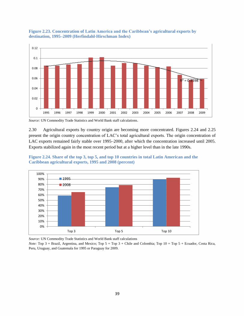
39

Figure 2.23. Concentration of Latin America and the Caribbean’s agricultural exports by

destination, 1995–2009 (Herfindahl-Hirschman Index)


2.30 Agricultural exports by country origin are becoming more concentrated. Figures 2.24 and 2.25

present the origin country concentration of LAC’s total agricultural exports. The origin concentration of

LAC exports remained fairly stable over 1995–2000, after which the concentration increased until 2005.

Exports stabilized again in the most recent period but at a higher level than in the late 1990s.

Figure 2.24. Share of the top 3, top 5, and top 10 countries in total Latin American and the

Caribbean agricultural exports, 1995 and 2008 (percent)

Source: UN Commodity Trade Statistics and World Bank staff calculations

Note: Top 3 = Brazil, Argentina, and Mexico; Top 5 = Top 3 + Chile and Colombia; Top 10 = Top 5 + Ecuador, Costa Rica,

Peru, Uruguay, and Guatemala for 1995 or Paraguay for 2009.

R² = 0.8598

0

0.02

0.04

0.06

0.08

0.1

0.12

1995 1996 1997 1998 1999 2000 2001 2002 2003 2004 2005 2006 2007 2008 2009

0%

10%

20%

30%

40%

50%

60%

70%

80%

90%

100%

Top 3 Top 5 Top 10

1995

2008

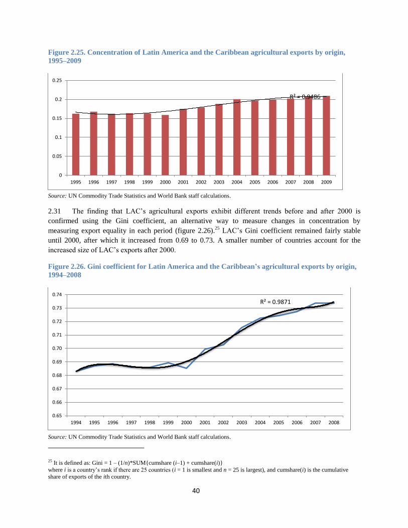
40

Figure 2.25. Concentration of Latin America and the Caribbean agricultural exports by origin,

1995–2009


2.31 The finding that LAC’s agricultural exports exhibit different trends before and after 2000 is

confirmed using the Gini coefficient, an alternative way to measure changes in concentration by

measuring export equality in each period (figure 2.26).25

LAC’s Gini coefficient remained fairly stable

until 2000, after which it increased from 0.69 to 0.73. A smaller number of countries account for the

increased size of LAC’s exports after 2000.

Figure 2.26. Gini coefficient for Latin America and the Caribbean’s agricultural exports by origin,

1994–2008


25 It is defined as: Gini = 1 – (1/n)*SUM{cumshare (i–1) + cumshare(i)}

where i is a country’s rank if there are 25 countries (i = 1 is smallest and n = 25 is largest), and cumshare(i) is the cumulative

share of exports of the ith country.

R² = 0.9486

0

0.05

0.1

0.15

0.2

0.25

1995 1996 1997 1998 1999 2000 2001 2002 2003 2004 2005 2006 2007 2008 2009

R² = 0.9871

0.65

0.66

0.67

0.68

0.69

0.70

0.71

0.72

0.73

0.74

1994 1995 1996 1997 1998 1999 2000 2001 2002 2003 2004 2005 2006 2007 2008

41

2.32 The product and destination trends over 1995–2009 reflect the strong growth of Brazilian and

Argentinean exports with an increasing concentration in products and a higher diversification in export

destination, a pattern shared by Chile, Uruguay, and Paraguay (table 2.2). Brazil and Argentina had the

most market equivalents and consistently increased the number of destinations over the period. Mexico,

however, kept a limited number of destinations, owing to its strong integration with its North American

Free Trade Agreement partners (the United States and Canada), and tended to have a stable and fairly

large set of products exported. Between these two extremes, the other LAC countries exhibited various

patterns in export diversification. Guatemala and Ecuador simultaneously increased their number of

products exported and markets reached; Colombia and Peru reduced their span of destination but slightly

increased product diversification.

42

Table 2.2. Product and destination diversification

Product

diversification

equivalent

number (1995)

(1)

Product

diversification

equivalent

number (2009)

(2)

Destination

diversification

equivalent

number (1995)

(3)

Destination

diversificatio

n equivalent

number

(2009) (4)

Product-destination

index equivalent

(1995)

(5) = (1)*(3)

Product-

destination

index

equivalent

(2009)

(6) = (2)*(4)

Latin

America

and the

Caribbean

4.1 3.4 11.7 17.0 48.3 56.9

Brazil 3.8 2.7 19.0 23.8 72.9 64.3

Argentina 2.1 1.7 15.8 27.1 33.6 45.0

Peru 3.0 3.3 12.4 11.3 37.7 36.9

Chile 3.2 2.9 9.4 10.1 30.4 29.0

Guatemala 2.2 3.2 5.8 6.7 12.6 21.4

Colombia 2.2 3.2 7.3 6.5 15.8 20.7

Uruguay 2.6 1.6 7.0 12.4 18.2 20.3

Ecuador 1.8 2.0 5.4 8.8 9.8 17.8

Bolivia 3.3 2.0 6.3 6.8 20.6 13.7

Costa Rica 2.3 2.3 5.4 5.9 12.3 13.5

Paraguay 2.7 1.2 3.7 9.9 10.0 11.6

Mexico 3.3 3.4 1.4 1.7 4.7 5.7


Note: The equivalent number is a theoretical value that represents the number of categories (product or destination markets) of identical size that

would lead to the degree of export concentration exactly equal to the one observed. It is defined as the inverse of the Hirschman-Herfindahl

Index. Calculating product differentiation through the equivalent number distinguishes for each country the equivalent number of exported goods

of equal importance (within the agricultural exports sector) leading to the same concentration of agricultural exports. The equivalent number

takes values between 0 and +∞. The larger the index value, the greater the export diversification in products or in destinations. Columns 5 and 6

are basically the product equivalent number multiplied by the destination equivalent number for 1995 and 2008, respectively. The index captures

developments in both the product and destination space. The data in columns 1–4 have been sorted according to the product destination index in

column 6.

2.33 Even though LAC’s overall agricultural exports showed greater market diversification but further

product concentration, there were great disparities among LAC countries. While the Southern Cone

countries deepened their specialization in producing meat, cereals, and oilseeds and reached more

markets, countries in Central America and the Andean regions reached more markets and diversified from

their original concentration in a few traditional products, especially coffee, bananas, and tropical fruits.

43

2.3.2 Value adding and moving up the value chain

2.34 Over 1994–2008, the share of world agricultural exports supplied by LAC countries increased by

about half, from 8 percent to almost 12 percent (figure 2.27).26

Figure 2.27. Latin America and the Caribbean’s share of world agricultural exports, 1994–2008

(percent)\

Source: Mandel (2012), based on UN Commodity Trade Statistics.

2.35 At the same time, the contribution of agricultural products to overall LAC exports fell by a third,

or about 10 percentage points, in line with the shrinking global share of agricultural trade (figure 2.28).

Dividing the agriculture share for LAC by that of the rest of the world yields a measure very close to the

revealed comparative advantage (RCA) index by Balassa (1965); the flatness of the ratio of the two series

(that is, LAC’s agriculture share is always about twice that of the rest of the world) indicates that LAC’s

overall RCA in agricultural goods remained fairly stable. Thus, overall LAC agricultural exports

consolidated global market share without a corresponding deepening in specialization.

26 This statistic was tabulated using the aggregates of a bilateral product-level trade dataset described below and includes trade

between countries within LAC.

VEGETABLES AND FRUIT (5)

COFFEE, TEA, COCOA,

SPICES AND

MANUFACTURES (7)

FEEDING STUFF FOR

ANIMALS (8)

FISH AND CRUSTACEANS

AND PREPARATIONS (3)

OIL SEEDS AND

OLEAGINOUS FRUITS (22)

TEXTILE YARN, FABRICS

AND RELATED PRODUCTS

(65)

MEAT AND MEAT

PREPARATIONS (1)

FIXED VEGETABLE FATS

AND OILS, CRUDE, REFINED

OR FRACTIONATED (42)

SUGARS, SUGAR

PREPARATIONS AND HONEY

(6)

0%

2%

4%

6%

8%

10%

12%

14%

1994 1995 1996 1997 1998 1999 2000 2001 2002 2003 2004 2005 2006 2007 2008

Sh

are

of

Wo

rld

Ag

ricu

ltu

ral E

xp

ort

s (%

)

44

Figure 2.28. Agriculture’s share of global and Latin America and the Caribbean trade, 1994–2008


Note: LAC = Latin America and the Caribbean.

2.36 But how could LAC’s share of agricultural markets rise and agriculture’s share in LAC and

global exports fall more or less in line with each other? One explanation could be that productivity (and

competitiveness) in LAC improved across the board in agriculture and nonagriculture sectors. Recent

research found that more productive and competitive exporters expand their market share by selling better

products, raising the question of whether quality upgrading could be behind the rise in LAC market share

for agricultural products.27

In a background paper for this study, Mandel (2012) addresses this question by

measuring agricultural export differentiation at the level of detailed products and finds limited evidence of

differentiated varieties within agriculture product groups. In other words, consistent with conventional

wisdom, agricultural exports are fairly homogeneous, and consequently there is limited space for

increasing value added by producing the same products but of better quality. Mandel then investigates a

second type of product upgrading, the manufacture of product groups with fairly high degrees of

processing and value added, to see whether interproduct upgrading accounts for part of LAC’s recent

market share increases. This study quantifies upstream and downstream specialization by defining which

industries are more input-intensive. It uses two methods to allocate industries to stages of production,

each with assumptions about agricultural industries’ input-output structure.

2.37 Conditional on the definitions of upstream and downstream industries, as well as on global trends

in specialization, LAC exporters have been tilting their specialization from upstream to downstream (that

is, more highly processed) industries. Specifically, LAC’s specialization in early-stage products is

growing more slowly than in the rest of the world, and its specialization in stage 2 products is growing

more rapidly. First, the textual descriptions of agricultural export products using Standard International

Trade Classification (Rev. 4) categories are used to infer their level of processing according to a set of

27 See Manova and Zhang (2012) and Harrigan and Baldwin (2011).

5%

7%

9%

11%

13%

15%

17%

19%

21%

23%

25%

27%

29%

31%

33%

35%

1994 1995 1996 1997 1998 1999 2000 2001 2002 2003 2004 2005 2006 2007 2008

Shar

e of L

AC

Exp

orts

Acc

ount

ed fo

r by

Agr

icul

tura

l Pro

duct

s

LAC Rest of World

45

keywords. For example, categories containing the words “prepared” or “processed” are assumed to be

farther downstream in the value chain of production than those containing the words “raw” or “fresh.”

Using these categories, LAC agriculture exports are more specialized in less processed, upstream stages

of production and there have been no consequential changes in specialization across stages over 1994–

2008. Figure 2.29 illustrates that both stage 1 and stage 2 categories contributed meaningfully to LAC

market share and LAC market share growth during that period. Stage 1 products accounted for 4.8

percent, or roughly 60 percent, of LAC’s agricultural market share in 1994, growing 2.3 percentage points

thereafter. Stage 2 products accounted for 3.2 percent of LAC’s market share in 1994, growing 1.2

percentage points thereafter. The relative growth contribution of products in the two stages maintained the

60/40 split between upstream and downstream export sales throughout the sample.

The second categorization scheme takes a more holistic approach of the input-output structure of

production by assigning stages to the entire set of industries from an input-output table, both agricultural

and nonagricultural. It utilizes the concept of forward flow, which is the amount of output from upstream

stages used as inputs to downstream stages minus the reverse flows of outputs from upstream stages used

as inputs to downstream stages. Industries are assigned to stages to maximize the overall forward flow

across all industries in the economy.28

These categories are applied to LAC export products. Interestingly,

and in contrast with the keywords classification, the net forward flow classification scheme indicates that

LAC is already more specialized in downstream products than in upstream products, though the extent of

downstream specialization has been declining (see figure 2.29). Over the course of the sample period,

stage 1 goods classified by net forward flow added 1.7 percentage points to LAC’s share of world

agricultural exports, similar to the 1.8 percentage points contributed by stage 1 products.

28 The ideal choice of input-output data to measure the net forward flow of LAC exports would be a set of industry-level matrices

for each LAC country. Unfortunately, input-output matrices at a level of detail close to the Standard International Trade

Classification 4-digit products used in the keywords classification are not publicly available for any LAC country. For this

analysis, two other input-output tables, for the United States and Thailand, are used to approximate the structure of production in

LAC. For each country, we use the input-output table to define stages of production, with industries allocated to stages to

maximize the economywide value of the net forward flow expression above. The key data used to define the production stages

are the 2002 benchmark input-output tables from the Bureau of Economic Analysis and the 2005 input-output table for Thailand.

46

Figure 2.29. Latin America and the Caribbean’s share of world exports by stage of production,

1994–2008 (percent)

Keywords classification Forward flow classification using a U.S. input-output table


2.38 The extent to which LAC exporters specialize in upstream or downstream products can be

examined by computing a Balassa RCA index of the following form for the nominal exports (X) for each

country (k) and each stage:

(

)

( )

2.39 This index is simply the country’s global market share in a stage divided by that country’s global

market share of total agricultural exports. According to classification of stages by keywords, because

LAC’s market share of stage 1 products is greater that its market share of stage 2 products, LAC’s stage 1

RCA will be greater than 1 and its stage 2 RCA will be less than 1; this is illustrated by the hatched lines

in figure 2.30. The market share of stage 1 products grew in line with their proportion, which made the

LAC RCA in each stage fairly stable over the sample period. Using the keywords classification, the

estimated degree of specialization is consistent with a standard narrative about resource-abundant

developing countries: their level of output depends heavily on primary goods with lower value added and

sophistication. Moreover, this classification does not indicate that specialization in stage 1 products has

given rise to an increasing proportion of exports of stage 2 products. Such a trend would be reflected in

the increasing RCA of stage 2 products and the decreasing RCA of stage 1 products. Using the forward

flow classification based on the U.S. input-output table, the slow growth of stage 2 products relative to

the level of their share means that stage 2 RCA fell from more than 1.45 in 1994 to 1.2 in 2008. Thus,

LAC specialization in downstream products according to this classification was high and decreasing. In

figure 2.30, this high level of stage 2 market share is almost exactly the opposite of LAC RCA as

measured by the keyword classification. But despite the different findings in the relative values of RCA

indices, the dynamics of comparative advantage by production stage remained consistent for LAC over

the study period. Using various structures of input-output relations, LAC increased its specialization in

upstream industries and reduced it for downstream industries.

Stage 1

Stage 2

0%

2%

4%

6%

8%

10%

12%

14%

1994 1995 1996 1997 1998 1999 2000 2001 2002 2003 2004 2005 2006 2007 2008

Sh

are

of

Wo

rld

Ag

ricu

ltu

ral E

xp

ort

s (%

)

Stage 1

Stage 2

0%

2%

4%

6%

8%

10%

12%

14%

1994 1995 1996 1997 1998 1999 2000 2001 2002 2003 2004 2005 2006 2007 2008

Sh

are

of

Wo

rld

Ag

ricu

ltu

ral E

xp

ort

s (%

)

47

Figure 2.30. Latin America and the Caribbean’s revealed comparative advantage by type

classification and stage of production, 1994–2008


2.40 The study also compared trends in LAC RCA in each stage of production with RCA trends in the

rest of the world. A common keywords classification and common (U.S.- and Thai-based) forward flow

classification to export products from all countries was uniformly applied. An important reason to

compare LAC trends with those of other exporters is to control for global trends in demand that can vary

by stage. For example, if China increases its imports of raw materials from all sources, all exporters

would appear more specialized in stage 1 products; this would not be very informative about the value

chain (production) dynamics that we seek to describe. The changes in RCA over time for each stage and

classification scheme are measured with the following panel regression:

∑

2.41 where LAC is a dummy for LAC countries and is an exporter fixed effect. can be

interpreted as the rate of specialization deepening in a given stage, while can be interpreted as the

relative rate of specialization deepening of exporters conditional on being a LAC country.

2.42 The estimated RCA trends for agricultural export products over 1994–2008 are shown in table

2.3. For stage 1, the estimates for are negative and significant regardless of the classification scheme.

This means that LAC RCA in stage 1 grew more slowly than RCA for stage 1 industries in the rest of the

world. Similarly, the point estimates for LAC’s specialization deepening in stage 2 are positive, though

only statistically significant for two of the three classifications. This indicates a faster rate of

specialization in stage 2 industries than that in the rest of the world. Together, these results suggest that

despite trends in LAC specialization toward upstream products, the composition of LAC exports relative

to other exporters has tilted toward downstream products. In contrast with , the estimates for are

sensitive to the classification scheme. While the keywords classification indicates that overall

specialization in stage 2 increased, both net forward flow classifications indicate the opposite.

Stage 1 (keywords)

Stage 2 (keywords)

Stage 1 (forward flow

- U.S. I-O table)


- U.S. I-O table)


- Thai I-O table)


- Thai I-O table)

0.6

0.7

0.8

0.9

1

1.1

1.2

1.3

1.4

1.5

1994 1995 1996 1997 1998 1999 2000 2001 2002 2003 2004 2005 2006 2007 2008

LAC'

s Rev

ealed

Com

para

tive A

dvan

tage

in St

age 1

& 2

Prod

ucts

48

Table 2.3. Trends in revealed comparative advantage (RCA) by stage in Latin America and the

Caribbean and the rest of the world

Source: Mandel 2012.

* significant at 5 percent; ** significant at 1 percent.

FE = Fixed Effect;

2.43 In this section, we analyzed the composition of LAC’s specialization patterns among products

with different degrees of processing. Using various methods to classify products as either upstream or

downstream, we show that both types of products have contributed meaningfully to LAC’s recent

increases in market share. Controlling for global specialization trends among upstream and downstream

products, LAC exporters are found to have deepened specialization in downstream products.

2.4 What has been driving the dynamos?29

2.44 LAC’s two biggest powerhouses, Argentina and Brazil, together accounted for around two-thirds

of the region’s export growth over 1995–2010. Both have lessons for other countries within LAC and

outside the region.

2.4.1 Argentina

2.45 Because of its favorable climate and natural endowments of land and water, Argentina has a

strong comparative advantage in temperate agricultural products and has long been a major producer and

exporter of grains and meat. Nonetheless, recurring macroeconomic mismanagement and anti-export and

anti-agricultural biases—created by import-substitution policies and export taxes and restrictions—led to

fairly stagnant production in the five decades leading up to the 1990s.

2.46 In the early 1990s, however, a package of reforms dramatically changed the policy environment

for agriculture. This was followed by a rapid expansion of agricultural area—grain and soybean area

increased by about half from crop years 1995/96 to 2005/06—and much more rapid expansion of

production, which increased around 225 percent (figures 2.31 and 2.32). General economic reforms that

affected agriculture and other sectors included:

29 This section is drawn principally from two papers sponsored by the FAO/CP program—O’Çonnor (2011) and Buanain and

others (2011)—and from Regúnaga 2010, commissioned as a background paper for this study.

Year -0.008 ** 0.005 ** 0.008 ** -0.011 ** 0.008 ** -0.007 **

(0.001) (0.001) (0.001) (0.001) (0.001) (0.001)

Year*LAC -0.010 * 0.008 ** -0.007 * 0.001 -0.009 **\ 0.010 **

(0.004) (0.003) (0.003) (0.004) (0.003) (0.003)

Exporter FE Yes Yes Yes Yes Yes Yes

Observations 3,559 3,565 3,567 3,558 3,564 3,566

R-squared 0.79 0.77 0.75 0.77 0.73 0.73

Net Forward Flow (Thai)

Stage 1 Stage 2

Dependent variable: RCA by exporter-stage-year

Keywords Net Forward Flow (U.S.)

Stage 1 Stage 2 Stage 1 Stage 2

49

Stabilizing domestic prices associated with the free convertibility of the currency and other sound

macroeconomic and fiscal policies implemented since 1991.

Implementing tax reform, including the elimination of taxes on production and trade.

Passing new legislation promoting foreign investment (no discrimination, bilateral investment

agreements with the main countries).

Eliminating quantitative restrictions on trade, price controls, and other nontariff barriers.

Privatizing public services, through the sale concession to the private sector of port and country

elevators, ports, highways, railways, energy, and other government-owned firms.

2.47 Other reforms were aimed specifically at the agricultural sector:30

Eliminating export taxes for most agricultural products. Export taxes were reduced from 41 percent

for soybeans in May 1989 to 20 percent in March 1990 with the new administration. In 1992, a 1.5

percent export tax earmarked for the National Institute for Agricultural Technology was eliminated.

Eliminating government intervention through the National Grain Board.

Promoting future markets for grains and oilseeds.

Opening the economy, including the reduction of import taxes on agricultural inputs and the

elimination of import taxes on capital goods. Elimination of quantitative restrictions on imports.

Creating the National Seed Institute (for intellectual property rights and seed quality controls) and the

new Seed Law to adapt to the International Union for the Protection of New Varieties of Plants

intellectual property principles.

Developing biotechnology policy to promote the development and use of genetically modified seeds,

including the creation of the CONABIA (Biotech and Biosafety National Organization) within the

Ministry of Livestock, Agriculture, and Fishing.

Strengthening the biotechnology programs in the National Institute of Agricultural Technology31

and

SENASA to improve food health issues.

Promoting (public and private) the use of no-till practices.

2.48 These reforms encouraged technology transfer by lowering barriers to importation of technology

embedded in inputs. It also spurred a competitive farm services industry and attracted investment that

improved the infrastructure for moving and storing grains. Innovative commercial arrangements emerged

to attract nontraditional financing into the sector, take advantage of economies of scale, and vertically

integrate the production chain to improve efficiency. As a result, aggregate factor productivity

increased—1.1 percent a year in agriculture and 0.9 percent in livestock—much more than in other

sectors, which increased 0.6 percent a year over 1990–2006.32

2.49 In recent years, however, some of these reforms—particularly trade policies—have been partly

reversed, shifting relative production incentives. Restrictions on corn and wheat exports combined with

30 Regúnaga 2010. 31 The National Institute of Agricultural Technology was created in 1956 to promote and strengthen the development of

agricultural research and extension and accelerate the benefits of these core functions: modernizing and improving agricultural

companies and rural life. It depends on the Ministry of Agriculture, Livestock, and Fisheries, with operational and financial

autarky. The institute’s main objective is to contribute to the competitiveness of agriculture, forestry, and agribusiness across the

country within a framework of ecological and social sustainability, generating information and technologies for processes and

products and putting them in the service of rural producers through the extension system. 32 Coremburg (2008), as cited in O’Çonnor (2011).

50

export taxes now create an effective tax rate higher than the soybean export tax. The uncertainty and high

level of export tax equivalent have induced farmers to reduce the area planted with corn and wheat and to

expand the area planted with soybeans. This is not good for soil rotation and conservation and increases

the risk of plant diseases associated with monoculture. The real impact on farms is much higher than the

nominal rate would suggest, because the prices at the farm level are much lower than at the ports.33

The

wedge between the farm-gate and free-on-board price is higher for products that are packaged or

processed off-farm than for those shipped in bulk. The export taxes thus create a special bias against these

high-value products and their associated processing industries, which can be significant sources of rural

employment. For example, the nominal tax rate of 10 percent on apple exports translates into a tax rate of

27 percent on apple production. And because the effective rate at the farm gate is magnified for regions

with higher transport costs to the ports, these taxes discriminate against the development of the regions far

from the ports. For example, under reasonable assumptions about prices and transport costs, a tax rate of

35 percent on soybean exports in Rosario could translate into a tax of 45 percent on production in Salta.34

2.50 Further increases in production and exports will depend on improving logistics and infrastructure.

Indeed, while most of the current infrastructure was built in the 1990s with little improvement in the

2000s, production has grown from 67 million tons in 2000/01 to around 102 million in 2010/11 (see

figure 2.32).

2.51 Export prohibitions on beef have likewise led to large reductions in the herd, from 56 million

head to 47 million in the last four years. Restrictions on milk exports and commercial controls have held

production at around 10 billion liters since 2000—after it increased 70 percent over the previous nine

years—despite a booming demand in world markets that generated rapid growth in production in Brazil

and Uruguay in the 2000s.

33 This is because the latter includes all the expenses needed for the transportation, conditioning, packaging, refrigeration, and

other expenditures associated with the added value. 34 Regúnaga 2011.

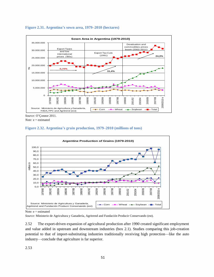
51

Figure 2.31. Argentina’s sown area, 1979–2010 (hectares)

Source: O’Çonnor 2011.

Note: e = estimated

Figure 2.32. Argentina’s grain production, 1979–2010 (millions of tons)

Note: e = estimated

Source: Ministerio de Agricultura y Ganadería, Agritrend and Fundación Producir Conservando (est).

2.52 The export-driven expansion of agricultural production after 1990 created significant employment

and value added in upstream and downstream industries (box 2.1). Studies comparing this job-creation

potential to that of import-substituting industries traditionally receiving high protection—like the auto

industry—conclude that agriculture is far superior.

2.53

Sown Area in Argentina (1979-2010)

0

5.000.000

10.000.000

15.000.000

20.000.000

25.000.000

30.000.000

35.000.000

1979

/80

1981

/82

1983

/84

1985

/86

1987

/88

1989

/90

1991

/92

1993

/94

1995

/96

1997

/98

1999

/00

2001

/02

2003

/04

2005

/06

2007

/08

2009

/201

0 e


FADA, FPC and Agritrend (est)

Ha


Export Tax Cuts

(1991)

Devaluation and

commodities prices

boom (2002-2011)Export Taxes

and low

international

prices ('80s)

-5,70%

31,4%

24,3%

Argentine Production of Grains (1979-2010)

0,0

10,0

20,0

30,0

40,0

50,0

60,0

70,0

80,0

90,0

100,0

1979

/80

1981

/82

1983

/84

1985

/86

1987

/88

1989

/90

1991

/92

1993

/94

1995

/96

1997

/98

1999

/00

2001

/02

2003

/04

2005

/06

2007

/08

2009

/201

0 e


Agritrend and Fundación Producir Conservando (est)

mill

ion

tn


52

Box 2.1. The soybean production chain in Argentina

The soybean production chain, with many different stages and participants, strongly influences employment and

regional consumption, especially for service providers. In recent years, the agroindustrial chain has become more

sophisticated and has promoted the development of several specialized industries. Some of them are high-tech, like

biotechnology and precision farming, and have created opportunities for new and more specialized jobs.

Several studies have estimated employment in the agribusiness sector and in specific value chains. Bisang and

Sztulwark (2007) studied employment in the soybean chain, from input providers to crushers (but excluding exports

and such related services as financing, quality services, and technical services). Using various assumptions, they

estimated a range of maximum and minimum jobs for each step and total direct employment of 215,000–304,000

jobs (box table 1). Most jobs are associated with total soybean acreage (14.5 million hectares) and production (32

million tons in 2003/04).

Using similar assumptions, our estimates for the 2007/08 crop (16.6 million hectares and 46.2 million tons) range

from 266,000 jobs to 381,000. This is several times the direct and indirect employment effects in protected

manufacturing industries, such as the automotive and spare parts value chain (from auto parts to distributors).

Following an approach similar to Bisang and Sztulwark’s, Castillo and others (2007) estimated total direct

employment in 2006 at 90,000: 57,600 for auto parts and vehicles, 18,400 for spare parts, and 14,000 for official

distributors.

Box table 1. Employment in the Argentine soybean chain, 2003/04

(number of jobs)

Most of the employment in the soybean

value chain involves small and medium-size

firms (primary producers, contractors,

country dealers, and carriers) based in towns

and small cities in the interior. Despite the

concentration of primary production and

crushing, the recent evolution of the industry

organization has been positive, providing

opportunities for the emergence and

development of local services and input

providers, members of an emerging middle class who live in small cities and towns in the main producing areas.

The regional distribution of firm owners and employees has been important to social and regional development,

stimulating local demand for products and services and improving regional welfare.

Source: Regúnaga 2010.

2.4.2 Brazil

2.54 Brazil is the world’s third-largest food exporter, after the United States and the EU. Even in a

period of rapid growth for the economy as a whole, there was no discernible declining trend in

agriculture’s contribution over 1994–2010 (figure 2.33); although highly variable from year to year, the

share remained around 6–8 percent. The share of agribusiness is much higher than that of primary

agricultural production and increased rapidly in the 2000s (figure 2.34), as did exports from the sector

(figure 2.35).

Steps / Participants Minimum estimate Maximum estimate

Seeds 1,250 1,250

Fertilizers and chemicals 1,878 10,500

Agricultural Machinery 19,350 23,000

Primary producers 91,498 108,500

Contractors 37,700 56,500

Country dealers - coops 36,961 55,035

Carriers 19,000 38,000

Crushers 7,000 11,000

TOTAL JOBS 214,641 303,786

53

Figure 2.33. Share in Brazilian GDP (percent) and value (R$) of Brazilian agricultural GDP, 1994–

2010

Source: Buainain and others (2011), based on Ipeadata.

Figure 2.34. Share in Brazilian GDP (percent) and value (R$) of Brazilian agribusiness GDP, 1994–

2010

Source: Buainain and others (2011), based on Cepea/USP/CNA 2011.

Figure 2.35. Trade balance—total and Brazilian agribusiness: 1989–2011 ($ billion)

Source: Buainain and others (2011), based on AgroStat.

54

2.55 As in Argentina, this rapid growth was stimulated by macroeconomic stability and sector reforms

put in place in the early to mid-1990s, which included trade liberalization (including elimination of export

taxes); virtual elimination of direct government purchase (including marketing boards); and deregulation

of markets for sugarcane, wheat, and coffee. Overall public spending in agriculture fell from 5.65 percent

of federal spending in the 1980s to 2.11 percent in 1995–99, but its composition improved as research

spending increased. Overall, Brazil’s Producer Support Estimate (as estimated by standard Organisation

for Economic Co-operation and Development methodology) rose from 0.92 in 1995–97 (indicating a net

tax of 8 percent on agriculture) to 1.03 (a 3 percent protection rate) in 2010.35

While overall support levels

are quite low, much of that support is provided through relatively distortionary instruments (price

supports, credit subsidies, and directed credit). The potential negative effects, however, are minimized by

limiting the support per farmer and targeting some payments (for example, making purchases from

“family farmers” at relatively high prices). While considerably less interventionist than in the past,

government agricultural policy continues to be activist in some areas, including rural finance.

Commercial banks are required by law to lend 25 percent of their sight deposits to agriculture. In

addition, the government has put in place two innovative programs to help farmers with finance and price

risk management (box 2.2). Increasingly in recent years, Brazil’s support programs are oriented toward

environmental goals: farmers qualify for some payments only if they respect agricultural zoning laws, and

support is planned for environmentally friendly cultivation practices. Even without special subsidies, a

very large fraction of Brazil’s land is cultivated using no- or low-till technology.

2.56 While Brazil has a large commercial farming sector that has received much government attention,

it also has many small family farms. Reforms in the mid-1990s initiated programs aimed at this sector.

The most important of these is the National Program to Strengthen Family Farms. The program includes a

number of subprograms, including a Harvest Guarantee Program, which provides farmers a minimum

payment in case of catastrophic crop loss due to weather. The guarantee covers only farmers in the

poorest regions. The government also started another weather insurance program for family farms in

2004, with wider coverage.

35 OECD 2011.

55

Box 2.2. Rural finance innovation has improved competitiveness

The Rural Producer Note (Cédula do Produtor Rural, CPR) was created by Law nº 8.929, August 22, 1994. It is a

private bond (promissory note) issued by farmers, farmers’ associations, and cooperatives. Through this note,

producers or farmers’ associations sell forward their production at a fixed price and agree to deliver the production

according to specifications defined in the note for quality, quantity, data, and place of delivery. The note is

endorsable and, if duly registered, fully negotiable. For countries at early stages of the development of commodity

exchange and derivatives markets—such as Brazil—investor acceptance of producers’ notes, commodity and

commercial papers, and other financial assets usually requires the intermediation (intervention) of a well-known

financial institution. Bank of Brazil is so far the only financial institution operating with CPR. It is not only helping

its clients issue and sell CPR but also guaranteeing the note itself. The bank charges its clients for the endorsement

and carries out regular auctions of CPR. Apparently, CPR has enormous potential to mobilize resources to finance

agricultural activities. It can be competitive with alternative financial assets and attract foreign investors familiar

with this type of operation. So far, however, its extent has been very limited, due to its expense and the fact that

producers bear all price risk.

In 1996, the government introduced options contracts, which may provide in the medium run an efficient instrument

for hedging against price risks. To introduce the option contract as an alternative for minimum price, the

government, through the Companhia Nacional de Abastecimento, or National Supply Company, is taking the role of

the speculator, technically called writer or seller of the option contract. While the buyer has the right to exercise the

option to buy or sell the commodity, the seller is the opposite party, which must stand ready to honor the contract in

case the buyer decides to exercise the option. In any case, the seller gets the premium paid for the option contract.

The supply company is selling options contracts for rice, maize, and wheat.

2.57 In addition to policy reform, technological innovation played a huge role in the Brazilian

experience. The federal research institute, EMBRAPA, was the most significant actor in this, but many

other private companies, universities, and research institutes also played important parts. EMBRAPA is

credited by many with developing the soil enhancement technology that transformed the vast area of the

cerrado from an agricultural wasteland to one of the country’s most productive areas.

2.58 The recent expansion of agricultural production differs from the dominant predatory pattern of

the 1960s and 1970s, when growth was sustained by the continual incorporation of new land into

production through deforestation.36

The occupation of the new frontier moved away from the traditional

cut-and-burn, shifting, and extensive production systems. It instead uses high investments and advanced

cultivation techniques that are more sustainable and environmentally friendly than traditional occupation

patterns, in which downgraded subsistence crops areas were replaced by pasture after three to five years

of cultivation.

2.59 Can Brazil maintain its position as the foremost developing country food supplier to world

markets? It has the resource base to do so. Brazil has 90–150 million hectares of unused arable land (a

conservative estimate) to sustain the increase in agricultural production without further deforestation. This

comprises mostly degraded pastures and savannah land with high potential for sustainable production.

Under the right production systems, its exploitation would have minor negative environmental impacts.

Besides, as Brazilian agricultural production is very heterogeneous, with many producers far from the

technological frontier, good opportunities for efficiency gains and productivity increases abound, in

systems from sugar cane to cattle breeding and even traditionally extractive crops.

36 Silveira and others 2005.

56

2.60 Notwithstanding the technical potential, sustainable growth depends fundamentally on the

availability of four additional factors: technology to sustain a vigorous innovation process and, in

particular, to cope with the threat of climate change; institutions to ensure appropriate incentives and

conditions for sustainable growth; infrastructure to reduce production costs, ensure favorable market

access, and create better conditions for integrating small and medium-size farmers in dynamic agrochains;

and microeconomic incentives and financial capital to fund investments at the farm level.

2.61 The geographic diversification of Brazilian agriculture during the last 35 years—and the legacy

of a closed economy that did not require efficient links to external markets—has created some bottlenecks

to agriculture competitiveness (particularly for grain crops) that the country will need to resolve to

continue supplying a large share of world markets. According to Barbosa and Nogueira Junior (2007), in

2005, road transport was responsible for 60 percent of the total volume of soybeans moved in the country,

rail for 33 percent, and waterways for 7 percent, while trucks were used to transport other grains. Silveira

and others (2005) highlight the stark differences among the main soybean-exporting countries in transport

efficiency and show that Brazil’s remains inferior to those of Argentina and the United States, its two

main competitors—because of the large average distance (more than 1,000 kilometers) between ports and

producer areas in the Center-West. According to estimates by Abiove, the high dependence on road

transport accounts for 60 percent of the total transported costs,37

exacerbated by the excessive number of

transshipments (three or more before reaching the port).

2.62 Another difference between main worldwide grain export countries relates to the storage facilities

network. Today’s deficit in bulk storage dynamic capacity in Brazil is an estimated 36 percent. With an

estimated 5 percent annual expansion of Brazilian agriculture by 2012, the need to expand port capacity is

estimated to be 560,000 tons a year, due to the need to increase moving capacity to 46.5 million tons of

grains.38

In Brazil, the storage network includes many intermediate storage facilities, private or owned by

cooperatives, outside of farm properties. According to Oliveira (2007), only 11 percent of Brazilian grain

storage facilities are located on-farm (40 percent in Argentina and 60 percent in the United States), with

53 percent in towns, 32 percent in rural villages and 5 percent in ports. These off-farm facilities have

substantial capacities, ranging from 30,000 to 60,000 metric tons. This generates economies of scale but

higher transaction costs between producers and intermediates and losses due to an excessive number of

transshipments. Additionally, more than 60 percent of the Brazilian logistics system is in the hands of a

few international corporations, like Cargill, Dreyfuss, and ADM.39

The poor quality of Brazil’s roads, the

deficit of rural storage capacity (estimated at 7–20 percent in static capacity terms), and the seasonal

nature of exports reduce Brazilian grain competitiveness, especially when prices are low.

2.63 Brazil places 61st on the Logistic Performance Index, which takes into account not only direct

transportation costs—freights, ports, and handling charges, fees, and side payments—but also induced

37 Silveira and others 2005. 38 Borges and others 2006. 39

These efforts would be counteracted by reducing the dynamic/static capacity relationship from seven a year to four, on

average, through an identity conservation system based on tests by the Cartagena Protocol on Biosafety to control live transgenic

transboundary flow between grain exporters and importers (Silveira and others 2005). Imposing unfriendly export procedures

leads to overregulation rents, inadequate market structure, and a lack of incentive to invest, resulting in low-quality, fragmented

services and frauds, though requiring new regulations. This consolidates the vicious logistic circle characterized by the World

Bank study (Arvis and others 2007).

57

costs, “hedging for the lack of predictability and reliability of the supply chain.”40

These costs stem

mostly from nondelivery or expensive measures to meet delivery schedules. Resolving this infrastructure

deficit is critical for the competitiveness of Brazilian agribusiness. This situation creates investment

opportunities for the private sector, but providing incentives to undertake them will require addressing

regulatory and institutional issues.

40 Arvis and others 2007, 16.

58

Chapter 3. The Enabling Environment for Agricultural Trade:

Potential Constraints and What Can Be Done to Overcome

Them

3.1. A region’s or country’s relative trade performance provides a summary measure of its global

market competitiveness. Chapter 2 looked at Latin America and the Caribbean’s (LAC’s) performance

indicators. But we also want to understand the underlying determinants of competitiveness, the most

constraining factors, and the policy levers that might overcome these constraints. Of course, many factors

determine competitiveness—including natural endowments and policies and investments that make on-

farm and in-factory production more or less efficient—some of which we considered in chapter 2. In this

chapter, we analyze determinants of trade competitiveness focusing on four areas directly connected to

trade policy: external market access (section 3.1); countries’ own trade policies, which may create anti-

agricultural and anti-export biases (section 3.2); regional trade agreements (section 3.3); and trade

logistics and infrastructure (section 3.4). We conclude in section 3.5 with policy recommendations

derived from the analysis.

3.1 External environment: barriers to exports from Latin America and the

Caribbean countries

3.2. An important determinant of the overall incentive structure for production and trade is the level of

barriers that a country’s exports face in trade partners’ markets. As with many developing countries, the

tariffs levied on exports of manufactured products from most LAC countries are lower than those on

agricultural exports. This creates an effective anti-export bias in the external environment for agriculture.

For some countries, the difference can be substantial.

3.3. But tariffs are not the whole story. Actual protection rates are sometimes lower than tariffs would

indicate because of “water” in the tariffs or exemptions and sometimes higher because of nontariff

barriers (NTBs). To take these factors into account, a background study for this report computed a Market

Access Overall Trade Restrictiveness Index (MA-OTRI).41

The MA-OTRI summarizes the impact of

other countries’ trade policies on each country’s exports. The index answers the following question: What

is the uniform tariff that, if imposed by all trading partners on exports of country c instead of their current

structure of protection, would leave exports of country c at their current level? The partial equilibrium

MA-OTRI is the weighted sum of protection levels (including tariffs and the ad valorem tariff equivalent

of domestic support payments and other NTBs) facing the exports of country c in other countries, where

weights are given by the elasticities of import demand in other countries and their imports from country c.

To obtain the ad valorem tariff equivalent of NTBs, the study first estimated the quantity impact of NTBs

on imports and then translated the quantity impacts into price effects, using the import demand elasticities

in Kee and others (forthcoming). This methodology can be used to estimate the real effect of tariffs

without the effect of NTBs. This measure is reported as the Market Access Tariff Trade Restrictiveness

Index (MATTRI).

41 See Kee and others (2009) for a detailed description and literature survey of trade restrictiveness indices.

59

Figure 3.1. Market Access Overall Trade Restrictiveness Index for Latin America and the

Caribbean exports by sector (percent)

Each bar is an index of the barriers to exports from the Latin America and the Caribbean to the region named below the bar.



AG = agricultural exports; MF = manufacturing exports; ALL = all exports


Figure 3.2. Market Access Tariff Trade Restrictiveness Index for Latin America and the Caribbean

exports by region (percent)

Each bar is an index of the barriers to exports from the Latin America and the Caribbean to the region named below the bar.



AG = agricultural exports; MF = manufacturing exports; ALL = all exports


3.4. Figures 3.1 and 3.2 show the trade restrictiveness indices (indicating market access barriers)

facing exports from LAC to regions on the horizontal axis, while figure 3.3 indicates the barriers facing

0.0%

20.0%

40.0%

60.0%

80.0%

100.0%

120.0%


LAC-All

LAC-AG

LAC-MF

0.0%

10.0%

20.0%

30.0%

40.0%

50.0%

60.0%


LAC-All

LAC-AG

LAC-MF

60

exports from each region (the bars) being imported into each region or country grouping on the horizontal

axis. Several conclusions can be drawn from these figures:

As comparing the MA-TTRI with the MA-OTRI demonstrates, NTBs have a substantial effect—in

many cases, more than doubling the effects of tariffs alone. For this reason, we focus on the MA-

OTRI in the subsequent discussion.

LAC agricultural exports face fairly high market access barriers, particularly in low-income countries

and South Asia. LAC manufactured products face lower barriers, indicating that agricultural exports

suffer from an anti-agricultural bias in external trade.

Figure 3.3. MA-OTRI for agricultural products by region (percent)

Each bar is an index of the barriers to exports from the region represented by the bar to the region or group of countries named

below the bar.




Globally, on average LAC’s agricultural exports face higher barriers (green bar above “All” in figure

3.3) than those of any other region except East Asia and the Pacific. While tariff barriers are relatively

low to agricultural trade within LAC, the overall restrictions facing LAC exports to other LAC

countries are relatively high (the green bar above LAC), indicating significant NTBs. This

corroborates the point made earlier that at least in agricultural products, regional—even

intraregional—agreements have not succeeded in reducing barriers to low levels.

LAC agricultural exports face the most severe market access restrictions in South Asia, followed by

the Middle East and North Africa, the EU, Europe and Central Asia, LAC, Sub-Saharan Africa, and

East Asia and the Pacific. The extremely high restrictiveness in South Asia mainly results from the

high tariffs and NTBs levied by India on Brazilian exports of raw cane sugar (with tariff of 60

percent) and undenatured ethyl alcohol (with tariff of 150 percent). LAC countries face significant

market access restrictions on their main agricultural exports of sugar, bananas, and rice, which are

among the most protected agricultural products in the world market.

Some of the Caribbean states (especially Guyana, St. Lucia, Dominica, and Cuba) face the highest

barriers—50–55 percent. Among the major exporters, Uruguay faces the highest barriers (close to 50

percent), followed by Brazil (about 35 percent). For country details, see the annexes.

0.0%

20.0%

40.0%

60.0%

80.0%

100.0%

120.0%


HI

EAP

ECA

LAC

MENA

SAS

SSA

61

3.2 Trade policies of Latin America and the Caribbean countries

3.5. An economy’s overall incentive structure for agriculture depends on its own policies as well as

those of its trading partners. LAC, along with other developing regions, followed an industrial-led import-

substitution strategy in the 1960s and 1970s, with high trade barriers protecting domestic manufacturing

industries and implicit or explicit taxation of agriculture. This created a significant anti-agricultural—and

anti-export—bias in these countries’ incentive structures. A careful multicountry study calculated the

relative rates of assistance42

to agriculture yearly since the mid-1960s. It found very negative rates in all

developing regions in the 1960s and 1970s (figure 3.4). However, in the 1980s many countries embarked

on structural reforms that began steadily eroding the anti-export and anti-agricultural biases. After several

decades of reforms, the incentive framework is now perhaps the least distorted in the world. Meanwhile,

many countries in Africa have continued to tax the sector, while developing countries in Asia have

followed the industrialized world in subsidizing agricultural production, though not to the same degree as

high-income countries. LAC stands out as the region in which the overall incentive structure has been

close to neutral since the early 1990s.

Figure 3.4. Relative rates of assistance at the regional level, 1965–2009

Source: Anderson and others for 1965–2004; authors’ own calculations for 2005–09, based on updated database for Anderson

and others (http://go.worldbank.org/5XY7A7LH40).

Note: The 2005–09 relative rate of assistance for Africa was heavily influenced by several countries (particularly Ethiopia) that

provided high positive protection to agriculture, but this is not representative of the continent. A majority of countries had

negative relative rates of assistance, as in earlier periods. Five-year weighted averages with value of production at undistorted

prices as weights. Latin America and Caribbean countries in the study were Argentina, Brazil, Chile, Colombia, the Dominican

Republic, Ecuador, Mexico, and Nicaragua.

3.6. But this is not the whole story. In many developing countries, trade policies and support programs

have been much more protective of import-substitute products than of exportables. The Anderson study

calculated the nominal rates of assistance to these two classes of goods and found a large and persistent

difference in almost all regions, creating an anti-export bias within agricultural policy (figure 3.5). LAC is

42 Relative rates of assistance measure the support through trade and exchange rate policy and budget support accorded to

agriculture, relative to similar support accorded to nonagriculture in the economy.

-50

-40

-30

-20

-10

0

10

20

30

1965-69 1970-74 1975-79 1980-84 1985-89 1990-94 1995-99 2000-04 2005-09 AFRICA

LAC

ASIA


62

no exception. Further, while nominal rates of assistance on exports have become less negative over time,

those for import-substitute products have grown more positive. Nonetheless, in LAC, this difference has

greatly diminished since the 1980s, indicating that the anti-export bias has been reduced. On balance,

while biases and distortions persist in some LAC countries—mainly favoring import substitutes over

export crops—the overall incentive structure is relatively conducive to an efficient agricultural supply

response to higher prices and appropriate investments.

Figure 3.5. Nominal rates of assistance for agricultural exportables and import substitutes in Latin

America and the Caribbean, 1965–2009

Source: Anderson and Valdes for 1965–2004; authors’ own calculations for 2005–09, based on updated database for Anderson

and others (http://go.worldbank.org/5XY7A7LH40).

Note: Five-year weighted averages with value of production at undistorted prices as weights. Latin America and Caribbean

countries in the study were Argentina, Brazil, Chile, Colombia, the Dominican Republic, Ecuador, Mexico, and Nicaragua.

3.7. As Krueger and others’ large study of agricultural policy underscores, macroeconomic policy in

many countries strongly influences the incentive structure facing agricultural production. Exchange rate

policy has often been used to implicitly tax the sector. In the 2000s, good macroeconomic policy in many

LAC countries generally maintained real exchange rates at levels much more stable than in the past,

avoiding large appreciations. In recent years, however, with booming commodity prices and recent

resource discoveries, exchange rates have begun to appreciate in important exporters (figure 3.6),

threatening the sector’s competitiveness. This trend may become more pronounced as resource production

ramps up.

-30.0

-20.0

-10.0

0.0

10.0

20.0

30.0

1965-69 1970-74 1975-79 1980-84 1985-89 1990-94 1995-99 2000-04 2005-09

Import-competing

Total

Exportables


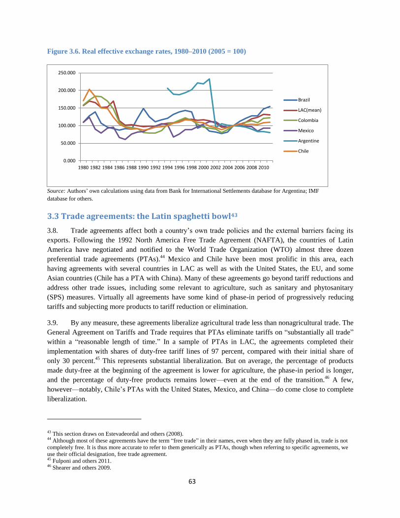
63

Figure 3.6. Real effective exchange rates, 1980–2010 (2005 = 100)

Source: Authors’ own calculations using data from Bank for International Settlements database for Argentina; IMF

database for others.

3.3 Trade agreements: the Latin spaghetti bowl43

3.8. Trade agreements affect both a country’s own trade policies and the external barriers facing its

exports. Following the 1992 North America Free Trade Agreement (NAFTA), the countries of Latin

America have negotiated and notified to the World Trade Organization (WTO) almost three dozen

preferential trade agreements (PTAs).44

Mexico and Chile have been most prolific in this area, each

having agreements with several countries in LAC as well as with the United States, the EU, and some

Asian countries (Chile has a PTA with China). Many of these agreements go beyond tariff reductions and

address other trade issues, including some relevant to agriculture, such as sanitary and phytosanitary

(SPS) measures. Virtually all agreements have some kind of phase-in period of progressively reducing

tariffs and subjecting more products to tariff reduction or elimination.

3.9. By any measure, these agreements liberalize agricultural trade less than nonagricultural trade. The

General Agreement on Tariffs and Trade requires that PTAs eliminate tariffs on “substantially all trade”

within a “reasonable length of time.” In a sample of PTAs in LAC, the agreements completed their

implementation with shares of duty-free tariff lines of 97 percent, compared with their initial share of

only 30 percent.45

This represents substantial liberalization. But on average, the percentage of products

made duty-free at the beginning of the agreement is lower for agriculture, the phase-in period is longer,

and the percentage of duty-free products remains lower—even at the end of the transition.46

A few,

however—notably, Chile’s PTAs with the United States, Mexico, and China—do come close to complete

liberalization.

43 This section draws on Estevadeordal and others (2008). 44 Although most of these agreements have the term “free trade” in their names, even when they are fully phased in, trade is not

completely free. It is thus more accurate to refer to them generically as PTAs, though when referring to specific agreements, we

use their official designation, free trade agreement. 45 Fulponi and others 2011. 46 Shearer and others 2009.

0.000

50.000

100.000

150.000

200.000

250.000

1980 1982 1984 1986 1988 1990 1992 1994 1996 1998 2000 2002 2004 2006 2008 2010

Brazil

LAC(mean)

Colombia

Mexico

Argentine

Chile

64

3.10. The dairy and sugar subsectors are particularly noteworthy for their very limited liberalization. In

general, PTAs with countries in Asia and Europe tend to have more exceptions to liberalization, though

this is not the case in the Chile–China and Transpacific (Chile–New Zealand–Singapore–Brunei) free

trade agreements. Many products exempt from duty-free status are subject to tariff-rate quotas, whereby

some limited quantity may be imported at a low or zero rate, with imports over this quota subject to a

higher—often the most favored nation—rate.

3.11. Most of these PTAs also have different rules of origin for agriculture. All PTAs have rules of

origin that exclude from preferential treatment goods not made with local inputs in the country exporting

them, so that exporters cannot import cheap products (or inputs) from a country outside the PTA and re-

export products (or products made with the imported inputs with only negligible value added) to a partner

in the PTA, taking advantage of the low duty. But these rules generally contain an exclusion granting

preferential treatment for products made with some imported inputs, as long as these inputs do not exceed

a threshold percentage of the good’s final value. (for most PTAs, 7–10 percent). However, many

agreements exclude agricultural products from this “general tolerance rule”—that is, they do not allow

agricultural products to benefit from the de minimis exemption.

3.12. SPS standards have become more stringent, a trend driven by consumer concern over chemicals

in the food chain and transmission of food-borne disease, as well as their potential for providing

nontransparent protection that is less constrained by WTO rules than other measures. As a result, these

standards are perhaps the most serious barrier to agricultural trade worldwide, making PTAs’ handling of

them highly relevant. A PTA provides an opportunity for partners to go beyond the minimal WTO

measures, particularly by operationalizing some core principles of the SPS Agreement: harmonization,

equivalence, regionalization, evaluation of risk and appropriate protection level, and transparency. Yet, in

a sample of recent PTAs involving LAC countries, 48 percent contained no provisions beyond the basic

WTO commitments, with only 52 percent categorized as “WTO Plus.”47

(For a summary of the details of

each country’s PTAs, see table A2.3 in annex 2.) Many WTO Plus agreements reside not in the PTA’s

basic text but in ad hoc agreements signed during its negotiation. But even some of these do not take full

advantage of the opportunity. For example, in an ad hoc agreement accompanying the Colombia–U.S.

free trade agreement, Colombia commits to recognizing as equivalent the U.S. inspection system for meat

and poultry and accepting the United States Department of Agriculture/Food Safety and Inspection

Service Export Certificate, notwithstanding U.S. outbreaks of mad cow disease. (The Peru–United States

agreement also did this.) Yet it did not provide similar benefits for Colombia, which had been trying for

two years to get the United States to accept regionalization, allowing meat exports to the United States

from regions of Colombia that had been declared free of foot-and-mouth disease.

3.13. A few agreements do include reciprocal commitments on other technical barriers to trade in

agriculture. NAFTA and the U.S. agreements with Chile and Panama, as well as Mexico’s agreements

with Costa Rica, Bolivia, and Nicaragua, commit both parties to respecting the principle of national

treatment on marketing requirements for packaging, grading, and sizes. NAFTA and Mexico’s other

agreements mentioned here also establish a committee or working group to review how these standards

affect trade and to resolve problems arising from them. Chile’s agreement with the United States is the

47 Shearer and others 2009.

65

only one in which a Latin American country receives a detailed commitment for mutual recognition of a

specific program— in this case, the grading program for beef.

3.14. Most PTAs call for phasing out export subsidies on agricultural products, with the conspicuous

exceptions of those with European countries, Israel, the Republic of Korea, and Japan, and those signed in

the 1990s with Mercosur and Central America. Many, however, do not specify a timetable for the phase

out. Slightly more than a third of the agreements regulate trade-distorting domestic support (for example,

from government budgets) to the agricultural sector. Also, more than a third of the agreements (all those

involving the United States and most involving Mexico and Chile) include provisions for safeguard

actions for some products, allowing the importing country, when faced with high import levels of a

product, to impose additional, temporary protection. Products most commonly mentioned in safeguards

are beef, pork, dairy, poultry, fruits, and vegetables.

3.15. So, have PTAs liberalized trade in agricultural products and improved member states’ welfare?

Notwithstanding the large number of PTAs, few robust (that is, generally applicable) answers have

emerged from research attempting to answer this question. This is due to several factors: the highly

specific nature of each agreement; difficulty establishing a counterfactual (what would have happened to

trade without the agreement) and thus causality; and the lengthy phase-in periods of many agreements

(especially for agricultural products), which delay their full implementation. Determining effects on

welfare is also complicated by the fact that even if a PTA clearly increased trade, it may have actually

reduced welfare if the trade was diverted—that is, if imports previously sourced from a very efficient

producer outside the PTA now come from a less efficient PTA member because tariffs were lowered with

PTA partners. This potential for diversion is one reason trade economists prefer multilateral trade

liberalization (WTO) and are skeptical of preferential agreements. In general, the higher the trade barriers

with countries outside the preferential area, the more serious the problem of trade diversion. Conversely,

the more globally competitive the trade partners within the agreement, the more trade will increase, not be

diverted.

3.16. One recent Organization for Economic Co-operation and Development (OECD) study of three

fairly long-standing PTAs—Mercosur, AFTA [the ASEAN Free Trade Agreement], and the Common

Market for Eastern and Southern Africa—concluded that they stimulated agricultural trade among

members and that the increased trade was not due to trade diversion. On the other hand, the agreements

did not increase trade with nonmember countries,48

a fact the study attributes at least in part to poor

infrastructure and supply constraints. Thus, the agreements have limited value. Another interesting study

of PTAs’ impact in LAC concluded that they have been building blocks to multilateral liberalization, with

a reduction of one percentage point in the preferential tariff in a free trade agreement, inducing a

reduction of almost 0.2 percentage point in the most favored nation tariff in the subsequent year.49

This

paper did not, however, look separately at agricultural products, which often receive special treatment in

PTAs.

48 Korinek and Melatos 2009. 49 Estevadeordal and others 2008.

66

3.17. A few in-depth studies have looked at PTAs’ effects on specific agricultural products. After

NAFTA took effect, corn exports from the United States to Mexico boomed, as expected.50

But, contrary

to predictions that low-cost imports would crush the domestic growers, production in Mexico (mostly

white corn) also grew substantially.51

This outcome arose partly because the imports, rather than

competing with domestic production, were absorbed by robust demand for yellow corn to use as livestock

feed; Mexican consumers consumed more meat, and exports of beef from Mexico to the United States

grew from around $274,000 in 1993 to $2 million in 1995 to $89 million by 2007.52

While this was

dwarfed by the growth in U.S. meat exports to Mexico, it nonetheless increased Mexican use of feed corn

substantially. And it is also clear that the agreement stimulated exports of fruits and vegetables from

Mexico to the United States. The effect of NAFTA-induced liberalization in the beans market was less

significant, due to the nature of bean demand in Mexico.53

And in the sugar market, NAFTA’s liberalizing

impact was attenuated, or at least delayed, by disputes and countermeasures.54

3.18. A case study of the Dominican Republic–Central America Free Trade Agreement (CAFTA-DR)

and the United States showed that the agreement greatly expanded fruit exports from the United States

and likewise greatly expanded exports from the CAFTA-DR countries to the United States of fresh fruits

and vegetables, some sweeteners, nursery products and flowers, and dairy products. On the other hand,

domestic political pressure from U.S. sugar producers resulted in severe constraints on liberalization in

that market, so the agreement is unlikely ever to have a significant impact on trade.

3.19. On balance, these case studies confirm the MA-OTRIs: notwithstanding the spaghetti bowl of

agreements among the LAC countries and with extraregional partners, agricultural trade barriers remain

relatively high for LAC exports, including within the region. For both intra- and extraregional trade,

NTBs are more significant than tariffs. PTAs will likely be more important for differentiated products

(processed products, fruits and vegetables, meats) than for standardized commodities—for two reasons.

First, for commodities, the price received by the exporter does not depend much on where (that is, in

which specific national market) the product is sold; what matters is the world market price. So

commodities blocked from one country by high tariffs or NTBs are still saleable to buyers in other

countries at the same price. For differentiated products, on the other hand, the price and the ability to sell

the product may depend heavily on market characteristics, so accessing the markets of specific countries

could be quite important. Second, tariff structures in most countries are escalated—that is, tariffs on more

processed products are higher—so there is more space for PTAs to improve access for the more processed

goods. The results of the gravity model reported in subsection 3.4.1 suggest this: while all subcategories

of agricultural exports show a significant positive effect of PTAs, the two with the highest coefficients are

processed products and meats. (The fact that bulks have a slightly higher coefficient than fruits and

vegetables seems odd, however.)

50 It is not entirely clear to what extent this can be attributed to NAFTA, because the government reduced barriers much faster

than required under the agreement. 51 World Bank/IMCO 2007a. 52 Shearer and others 2009. 53 World Bank/IMCO 2007b. 54 World Bank/IMCO 2007c.

67

3.4 Logistics and trade facilitation

3.20. Agricultural products’ competitiveness depends on many factors, from the field to the port. But

one critical area is the efficiency of the related logistics systems and the ability to connect effectively and

reliably to global supply chains. This section overviews the logistics challenges facing LAC countries and

corresponding recommendations for how to tackle them. Much of this report focuses on export products,

for which low logistics costs and good trade facilitation mean higher producer prices and greater

competitiveness in world markets. But given food’s importance to the poor, improving logistics and

facilitation can also help reduce poverty by keeping prices lower for imported foods. This is especially

critical in an era of very high prices for many staples.

3.21. In the past, when formal agricultural trade barriers were high, logistics costs were often

considered of secondary importance. But now that many of these formal barriers have been reduced—

though not nearly as much for agriculture as for manufactures—these “behind the border” and

international transport costs are increasingly being recognized as impediments to trade. For LAC in

particular, logistics and transport costs are two to three times greater than tariffs and duties. Average

import tariffs for LAC have declined since the early 1990s and remain at an average of about 11 percent.

National average logistics costs, however, represent a share of product value of 18–32 percent, well above

the OECD benchmark of around 9 percent (figure 3.7). The international maritime and road haulage

components alone can total about 20 percent of the free-on-board value of goods. By the time products

are transferred, handled, stored, and distributed domestically, the logistics component of the delivered

good is often more than 50 percent of the final price to consumers, twice the levels of OECD countries.

Figure 3.7. Logistics costs in Latin America and the Caribbean and in Organization for Economic

Co-operation and Development countries, 2004

Source: Guasch, 2011

3.22. In this section, we look at the importance of trade facilitation and logistics from two perspectives.

Subsection 3.4.1 takes a macro or “bird’s-eye” look at the importance of these factors in agricultural

trade. It uses an augmented gravity model of trade to quantify the impact of various trade facilitation

indicators on countries’ export performance, with a focus on LAC agricultural exports. It also looks

broadly at what improvements would be most useful for agricultural and nonagricultural trade and for

particular kinds of agricultural products. And finally, relying on the findings from the gravity model, it

quantifies what impacts on trade would result from improving LAC policies and infrastructure to OECD

standards. Subsection 3.4.2 then delves deeper at a more micro level to look at specific challenges faced

by different LAC countries, benchmarking them against each other and against other regions. For this, the

68

analysis relies on a variety of micro-level studies and surveys, including some very detailed studies of

supply chains in Latin American countries. Subsection 3.4.3 concludes this chapter with policy

implications.

3.4.1 How important is trade facilitation?55

3.23. Trade facilitation consists of policies to reduce trade costs so that firms can expand their export

volumes and reach new markets. We use two aggregate indicators developed by Portugal-Perez and

Wilson (2012) to measure the trade facilitation environment in each country. The first indicator quantifies

the quality of the physical infrastructure, such as ports and roads, also known as hard infrastructure. The

second indicator measures the overall quality of the regulatory and business environment, or soft

infrastructure. In addition, we use the number of days to export as a proxy for the overall logistics in each

country. The number of days to export is a good measure of both inside-the-border and at-the-border

obstacles and controls for possible complementarities between hard and soft infrastructure.

3.24. Using the estimates in the gravity model described below, we simulate the impact of enhanced

trade facilitation, measured by higher indicators, on exports expansion in each LAC country. The results

are clear: if LAC countries could achieve the trade facilitation levels of the average OECD country, the

region could increase agricultural exports around 140 percent and total exports nearly 100 percent. This

finding is consistent with a broad range of other studies that have shown the value of both hard and soft

infrastructure.56

By distinguishing soft infrastructure from hard infrastructure we can compare the benefits

of investment or policy reform along both dimensions.

3.25. Constructing trade facilitation indicators. Recent empirical research has used many trade

facilitation indicators at the country level and with extensive geographic coverage to estimate their impact

on trade. From an econometric point of view, including variables of trade facilitation, measuring similar

aspects on the right-hand side of a model, such as a gravity specification, can be conducive to

multicollinearity. To circumvent multicollinearity, we can reduce the dimension of the data by

aggregating highly correlated indicators into a single indicator. With this in mind, a background study for

this report borrowed two aggregate trade facilitation indicators derived by Portugal-Perez and Wilson

(2012)57

using factor analysis: physical infrastructure and business and regulatory environment. Both

indicators are standardized on a scale ranging from 0 to 1, with 1 being the best-performing country.

3.26. As a proxy for hard infrastructure, physical infrastructure measures overall infrastructure

development and quality and is derived from four primary variables compiled from the World Economic

55 This section is drawn largely from a background paper for this study, “Trade Facilitation in Latin America and Agricultural

Exports,” by Esteban Ferro and Alberto Portugal-Perez, both of the World Bank. 56 On the value of institutional quality in improving trade performance, see Levchenko (2004), Anderson and Marcoullier (2002),

Ranjay and Lee (2003), and Depken and Sonora (2005). On the role of infrastructure and business environment, see Limao and

Venables (2001), Wilson and others (2003, 2005), Djankov and others (2006), Francois and Manchin (2007), and Portugal-Perez

and Wilson (2012). 57 Portugal-Perez and Wilson (2012) derive four new aggregate indicators of trade facilitation from a wide range of primary

indicators using factor analysis, a statistical modeling technique that explains the correlation among a set of observed variables

through an unobserved “common factor.” The new aggregate indicators contain the information of a wider range of individual

indicators than previous studies and focus on factors related to the hard or soft dimension of trade facilitation. The indicators are

derived for 101 countries over 2004–07, greater and more recent coverage than previous indicators. The indicators are derived

from a pool of 20 primary indicators collected from different sources: Doing Business, the World Development Indicators, the

World Economic Forum, and Transparency International.

69

Forum: quality of ports infrastructure, quality of airports infrastructure, quality of road infrastructure, and

quality of railroad infrastructure.

3.27. As a proxy for soft infrastructure, business and regulatory environment measures the

development level of regulations and transparency. The synthetic indicator is derived from five simple

indicators from the World Economic Forum and one indicator from Transparency International. The

World Economic Forum indicators are public trust for governments, irregular payments in exports and

imports, irregular payments in public contracts, measures to combat corruption, and favoritism of

government to well-connected firms. The Transparency International indicator is government

transparency.

3.28. Gravity model. The study used a gravity model to assess the impact of trade facilitation on trade

flows.58

The gravity model of international trade flows is a common approach to model determinants of

bilateral trade flows. The standard gravity formulation includes measures of market size (that is, GDP,

population), measures of remoteness (distance and adjacency), and measures of kinship (regional trade

arrangements and language or ethnic similarities). The study augmented the basic model to include tariffs

as well as the trade facilitation indicators and some additional controls. More precisely, it estimated the

following specification:

ijjijijijij

ijijii

ijiiiij

PTAceDisPopulationGDPpc

tdaysExportInfraSoftInfraHardX

ColonizerCommonColonyLanguageBorderREER

LACtanln)ln()ln(

1ln)ln()ln()ln(ln

111098ij7

i65432

13210

(1)

3.29. where Xij is country i’s exports to country j; Hard Infrai and Soft Infrai are our two infrastructure

indicators for country i with higher values representing better performance; Export daysi is the number of

days it takes a standard cargo to move from the factory gate to the ship; tij, are tariffs on imports of

country j from country i; REER is the real exchange rate; PTAij is a dummy equal to 1 when countries i

and j have an active preferential trade agreement; LAC is a dummy equal to 1 when the export is a LAC

country; Borderij, Common Languageij, Colonyij, and Common Colonizerij are dummy variables that are

equal to one if countries i and j, respectively, have common border, common language, same colonizers,

and common colonizers post-1945. Finally, j is a vector of importer-specific fixed effects, whereas Ɛ ij

is a random error term.59

58 Gravity models are mathematical models based on an analogy with Newton’s gravitational law and used to account for

aggregate human behaviors related to spatial interaction, such as migrations, traffic, and trade flows. The gravity model states

that the volume of trade can be estimated as an increasing function of the national incomes of trading partners and a decreasing

function of the distance between them. Although the model’s ability to predict trade flows has been popular for several decades,

only recently has it been supported with theoretical foundations. These studies show that estimates can be derived from various

theoretical frameworks, such as the Ricardian, Heckscher–Ohlin, and increasing returns to scale models. Theoretical foundations

for estimating gravity equations were developed by Anderson (1979) and enhanced in Anderson and van Wincoop (2003, 2004). 59 A complete specification would also require fixed effects for exporters to control for multilateral resistance terms, but their

inclusion would wipe out the effect of exporter-specific variables, including our variables of interest, hard and soft infrastructure.

70

3.30. Data. The dataset covers 100 exporting countries and 137 importing countries over the period

2005–08, as most of our trade facilitation indicators only cover this period.60

Aggregate trade flows were

compiled from the United Nations Commodity and Trade Database (COMTRADE), whereas applied

tariffs were compiled from the UNCTAD Trade Analysis and Information System (TRAINS) database.

Core gravity variables, such as bilateral distances, colonial ties, and common language dummies were

obtained from the Centre d’Etudes Prospectives et d’Informations Internationales website. Compiled

from Penn World Tables, the real exchange rate is defined as the exporter’s nominal exchange rate

deflated by the country’s consumer price index over the importer’s nominal exchange rate deflated by its

consumer price index. Other relevant variables, such as GDP and population, were available from the

World Bank’s World Development Indicators. As mentioned, the aggregate trade facilitation indicators

for each exporter were taken from Portugal-Perez and Wilson (2012) and the days to export in each

country were taken from the World Bank’s Doing Business survey.

3.31. Estimation and results. Table 3.1 reports estimates for the gravity model defined by equation (1),

with each regression having three dependent variables—total exports, industrial exports, and agricultural

exports—to evaluate the differentiated impact of each type of export to changes in the trade facilitation

environment. In column 1, both hard and soft infrastructure have positive and significant coefficients, as

improving both areas of trade facilitation would result in greater exports. The coefficient on the number

of days to export is negative and significant, as a reduction in the time that a shipment takes from factory

release to board shipment is associated with higher exports. The coefficient of the real exchange rate

(REER) is positive, as depreciation in the currency is associated with exports surge. The positive and

significant coefficient for the LAC dummy means that, all else equal, LAC countries export more than the

average country.

3.32. The remaining traditional variables in gravity models have signs and magnitudes consistent with

the literature. Indeed, higher tariffs, as well as longer distances between partners, discourage trade. By

contrast, the trade volume is higher between partners in a regional trade agreement, as well as between

richer and more populous countries. Contiguous partners, countries with a common official language, and

countries having had a common colonizer or a colonial relationship are also likely to trade more

intensively.

3.33. Estimates for specifications explaining industrial exports and agricultural exports reported in

columns 2 and 3 of table 3.1 are fairly similar to estimates explaining total exports in column 1. Yet the

greater difference is in the magnitude of coefficients for trade facilitation, as hard infrastructure has a

greater impact on industrial exports, whereas soft infrastructure has a greater impact on agricultural

exports.61

In addition, increasing the number of days to export has a higher impact on agricultural exports

than on industrial exports, because most agricultural products are perishable. Preferential tariff

agreements have a greater impact on agricultural exports, whereas real exchange rates have a greater

60 Because there is almost no variation across time for the explanatory variables, we decided to aggregate data across time and do

a cross-section analysis in which the variation comes from the difference between countries in trade flows and explanatory

variables. 61 The coefficients estimated in the industrial and agricultural regressions (that is, columns 2 and 3 of table 3.1) are statistically

different from each other with the exception of days to export.

71

impact on industrial exports. The LAC coefficient is higher for agricultural exports than for industrial

exports, which indicates LAC’s comparative advantage in agriculture.62

Table 3.1. Gravity model estimates

Gravity Model Estimates (1) (2) (3)

Dependent Variable ln(total_exp) ln(indus_exp) ln(agro_exp)

ln (hard infra) 1.077 1.304 0.408

[0.067]*** [0.070]*** [0.109]***

ln (soft infra) 0.163 0.12 1.079

[0.052]*** [0.055]** [0.080]***

ln (1+tariff) -1.028 -1.646 -1.998

[0.341]*** [0.349]*** [0.341]***

PTA (d) 0.235 0.276 1.296

[0.064]*** [0.067]*** [0.096]***

REER 0.021 0.024 -0.011

[0.004]*** [0.005]*** [0.007]

LAC (d) 0.568 0.171 1.571

[0.053]*** [0.055]*** [0.078]***

ln (exp gdpcap) 1.026 1.224 0.432

[0.022]*** [0.023]*** [0.033]***

ln (exp population) 1.273 1.297 1.180

[0.012]*** [0.013]*** [0.019]***

ln (distance) -1.348 -1.460 -1.021

[0.032]*** [0.032]*** [0.049]***

Border (d) 0.916 0.900 1.130

[0.126]*** [0.131]*** [0.154]***

Language (d) 0.610 0.560 0.837

[0.058]*** [0.058]*** [0.083]***

Colony (d) 0.422 0.422 0.895

[0.107]*** [0.114]*** [0.135]***

Common Colony (d) 0.835 0.964 0.347

[0.084]*** [0.083]*** [0.117]***

Constant -12.857 -13.190 -10.012

[0.538]*** [0.591]*** [1.591]***

Observations 12,948 12,814 9,641

R-squared 0.776 0.782 0.524

Robust standard errors in brackets clustered by exporter-importer pairs.

* significant at 10%; ** significant at 5%; *** significant at 1%. (d) for dummy

variable. All regressions include importer fixed effects.

62 As there is no control for zero-trade in these regressions, any existing selection bias would tend to be greater in the agroexport

regression, because only 70 percent of the possible importer-exporter combinations actually trade, whereas for total and industrial

exports almost 94 percent of the possible country pairs have nonzero trade flows. We tested for the seriousness of this bias. A

partial correction for selection and firm heterogeneity bias shows that the results are nearly identical to the ones reported—

evidence that the bias is small for our sample.

72

Table 3.2. Agricultural exports by product type

Agricultural Exports by Product

(1) (2) (3) (4) (5) (6)

Total Agro Meat Bulks

Fruits &

Veg Agro-ind Other Agro

ln (hard infra) 0.778 0.855 0.931 0.942 0.829 0.299

[0.113]*** [0.162]*** [0.163]*** [0.154]*** [0.132]*** [0.138]**

ln (soft infra) 1.011 0.628 0.586 0.845 0.693 1.017

[0.080]*** [0.117]*** [0.120]*** [0.138]*** [0.091]*** [0.108]***

ln (arable land) 0.198 0.246 0.743 0.072 0.049 -0.062

[0.029]*** [0.038]*** [0.042]*** [0.041]* [0.031] [0.038]

ln (water reserves) 0.225 0.338 0.124 0.092 0.138 0.297

[0.022]*** [0.028]*** [0.032]*** [0.028]*** [0.023]*** [0.027]***

ln (1+tariff) -2.089 -1.554 0.587 -0.145 -2.300 -1.930

[0.347]*** [0.621]** [0.576] [0.567] [0.434]*** [0.426]***

PTA (d) 1.044 0.844 0.778 0.719 1.262 0.714

[0.099]*** [0.126]*** [0.136]*** [0.130]*** [0.100]*** [0.119]***

REER -0.011 -0.048 0.019 -0.012 -0.020 -0.032

[0.007] [0.012]*** [0.010]* [0.009] [0.009]** [0.009]***

LAC (d) 1.290 1.114 1.071 1.407 1.336 1.097

[0.083]*** [0.122]*** [0.131]*** [0.116]*** [0.088]*** [0.106]***

Observations 9,297 5,383 5,377 5,495 7,220 6,514

R-squared 0.541 0.431 0.415 0.437 0.531 0.432 Dependent variable is the natural logarithm of exports for the group of products in each column header.

Robust standard errors in brackets clustered by exporter-importer pairs. * significant at 10%; ** significant at 5%;

*** significant at 1%. (d) for dummy variable. All regressions include importer fixed effects. All regressions include

all gravity variables but are omitted from the table due to space constraints.

3.34. Table 3.2 shows the results of a gravity model of trade in which the dependent variables are

exports of several subcategories of agricultural products.63

As the dependent variables are exports of

agricultural goods, we include two additional controls—hectares of arable land and total renewable water

sources available in a country—as proxies for factor endowments intensively employed in agricultural

production.64

As a benchmark, we report estimates for total agricultural exports in column 1 of table 3.2.

Estimates show that trade facilitation is relevant for exports of all agricultural categories. Indeed, the

coefficients of hard and soft infrastructure are positive and statistically significant in all regressions,

whereas number of days to export is always negative and statistically significant. The results are fairly

consistent with previous findings: exports of heavier products such as industrial products and “bulks”

depend more on the quality of hard infrastructure, whereas time-sensitive products depend more on soft

63 The subcategories of agricultural products are defined by the following harmonized system categories. Meats: HS 02-04.

Bulks: HS 10-12. Fruits and vegetables: HS 06-08. Agro industry: HS 16-24. Other agro: HS: 05, 09, 13–15. 64 Arable land was taken from the World Development Indicators and total renewable water source from FAO Aquastat.

73

infrastructure and clearly on number of days to export. For example, exports of meats, a highly perishable

product, are extremely sensitive to time delays.

3.35. Simulations. The study also assessed the impact of a potential improvement of trade facilitation

indicators for each LAC country to the level of the average OECD on total exports, industrial exports, and

agricultural exports by simulating the gravity models estimated in table 3.1.

Figure 3.8. Increase in exports from an improvement in hard infrastructure to the Organization for

Economic Co-operation and Development level (percent)

Source: Background paper for this study by Ferro and Portugal

3.36. The average OECD measure of hard infrastructure in our sample is 0.77, compared with the

average LAC hard infrastructure measure of 0.35. The exercise performed for figure 3.8 is to assume that

each country in LAC improves its quality of hard infrastructure to receive a mark of 0.77. Every country

in LAC would benefit from such an improvement. The average increase in LAC exports from an

improvement in hard infrastructure to the level of OECD countries is 106 percent for total exports, 133

percent for industrial exports, and 28 percent for agricultural exports. While the specific quantitative

estimates cannot be taken too seriously, clearly the benefit of an improvement in hard infrastructure

would be greater for industrial exports than for agricultural exports.

0%

100%

200%

300%

400%

500%

600%

ARG BOL BRA CHL COL CRI ECU GTM GUY HND JAM MEX NIC PAN PER PRY SLV URY VEN LAC


74

Figure 3.9. Increase in exports from an improvement in soft infrastructure to the Organization for

Economic Co-operation and Development level

Source: Background paper for this study by Ferro and Portugal-Perez

3.37. Figure 3.9 shows the results of an improvement in the soft infrastructure indicator to the level of

the OECD average. The average soft infrastructure measure for LAC is 0.31, whereas the average grade

for the OECD countries is 0.76. Achieving a grade in soft infrastructure as good as that available in

OECD countries will more than double LAC’s agricultural exports. Again, the specific numbers cannot be

taken too seriously, but the exercise indicates that even though the impact of improving soft infrastructure

is not as strong as that of improving hard infrastructure in total exports, it proves to be overwhelmingly

important for agricultural exports. These estimates illustrate trade facilitation’s importance. However, two

points should be kept in mind. First, the gravity model does not consider any cost variable; therefore, we

cannot base any policy recommendation that would flow from a cost-benefit analysis on this type of

model. Clearly, the cost of improving, for example, Bolivia’s hard infrastructure to the level of the

average OECD country will be exorbitant and bring diminishing returns to investment. The main purpose

of this exercise is to identify trade constraints in LAC countries relative to other countries. Second, the

large effect of trade facilitation on trade does not result from mistaking the relationship between

facilitation and trade as linear. Because these effects seemed quite large, we tested for the possibility of

diminishing returns to trade facilitation by including a squared term for each trade facilitation variable.

The coefficient on each squared term was positive (negative for days to export), indicating increasing

rather than diminishing returns to trade facilitation. Thus, though large, our simulations’ results are

statistically conservative.

3.38. Another way to measure this effect is to estimate the tariff concessions that LAC countries would

need to obtain from their trading partners to achieve a level of agricultural exports equal to those reached

with the improvement in the trade facilitation measures simulated above. To illustrate how these

counterfactuals are estimated, suppose that an investment in port infrastructure of an exporter country

leads to a 1 percent increase in the hard infrastructure indicator. This leads to a change in trade flows of

0%

100%

200%

300%

400%

500%

600%

700%

800%


75

about ̂ percent, according to the gravity estimates.65

The same change in trade flows would be

brought about if all importers were to cut the tariffs applied to imports from the country by an equivalent

value ̂ ̂ .. Therefore, the latter ratio roughly represents the “ad-valorem tariff-cut

equivalent” or “ad-valorem equivalent” of a 1 percent change in the cost of export procedures inferred

from gravity model estimates.

Figure 3.10. Ad-valorem tariff-cut equivalents

Source: Background paper for this study by Ferro and Portugal-Perez

3.39. The results are reported in figure 3.10. Expansion of agricultural exports from improving hard

infrastructure quality to the level of the average OECD country would also be feasible with a reduction of

13.5 percent in tariffs in importing countries. If the improvement is made in soft infrastructure quality, the

ensuing expansion of agricultural exports would be feasible with a tariff reduction of 68.7 percent.

However, for many countries the tariff concessions needed to achieve the levels of exports achieved by

improvements in soft infrastructure are more than 100 percent, which would be equivalent to an import

subsidy from trading partners.

3.4.2 Agricultural trade logistics in Latin America and the Caribbean: benchmarking and

breaking it down66

3.40. As we saw in subsection 3.4.1, the big picture is that trade logistics—both hard and soft

infrastructure—matter a lot for agriculture and deserve to be at or near the top of the trade policy priority

list. But to transform this overarching policy message into an actionable agenda requires seeing how close

the region is to best practice elsewhere to assess the potential for improvement and looking at logistics at

a more granular level, both more focused on specific logistics and facilitation measures and more country-

65 For notation purposes, let ̂ be the estimated elasticity of imports with respect to the variable X entering in the gravity

equation. In the case of Doing Business days to export, the estimates should be negative. 66 This subsection is drawn largely from a background paper by Gwyn Fries, Jordan Schwartz, and Adam Stern.

0%

50%

100%

150%

200%

250%

300%

350%

400%

ARG BOL BRA CHL COL CRI ECU GTM GUY HND JAM MEX NIC PAN PER PRY SLV URY VEN LAC

TF Infrastructure TF Business

76

specific. In this subsection, we compare LAC countries to other regions and countries in overall

performance and identify priority areas for improvement according to subregion and country.

3.41. The logistics chain has many links, and inefficiencies in any of them fall disproportionately on

poor consumers and small producers. There are many aspects to logistics and trade facilitation—services,

physical infrastructure, and procedures. The main logistics components discussed in this chapter are

illustrated in figure 3.11.

Figure 3.11. Typical logistics chain for agriculture exports

Source: Adapted from Schwartz and others (2009).

3.42. And, while we saw in subsection 3.4.1 that LAC does not stack up well to the OECD countries,

there is a wide range among LAC countries. For example, food logistics costs for Peru, Argentina, and

Brazil are greater than 26 percent of product value, while Chile, a regional leader in logistics, has costs of

about 18 percent, still double that of the OECD (figure 3.12).

Figure 3.12 Logistics cost as percentage of food product value, 2004 (percent)

Source: Gonzales and others 2008.

3.43. Although the logistics burden affects consumers, importers, and the competitiveness of LAC’s

firms across the region, the impact is greatest on the region’s poor consumers and on small producers.

Food expenditures make up a large part of the disposable income of the region’s poor. Across income

Services

Infrastructure

Trucking from farm

gates and production

zones to ports/airports

Cargo handling, storage, consolidating and forwarding

Ocean shipping: bulk and containerized

Procedures Transit regulation, municipal taxes, and letters of credit

Roads, rail roads, airports,

silos, refrigeration

storage, and warehousing

Customs, inspections,

phytosanitary

clearances and

fumigation

Border crossing:

lanes, scanners,

storage area

Ports: berth, cranes, apron, wharf, container storage

Container security,

insurance

1. Inland transport

2. Points of import/export

3. Maritime transport

77

levels in LAC, food is the primary purchase of households, accounting for 20–30 percent of all spending.

The poor, however, spend up to 70 percent of household income on food. Further, about half the region’s

poor are now urban dwellers, no longer able to rely on subsistence farming.

3.44. Small firms, which are the majority of firms in LAC countries and the region’s employment and

growth engines, also suffer disproportionately from high logistics costs.67

Perishable agricultural products

have unique characteristics that require specialized logistics systems, including remote production zones,

temperature control, and special sanitary inspection procedures. Because of the time sensitivity of

perishable agricultural goods, bottlenecks in the logistics system directly affect the quality and quantity of

goods delivered. For nonperishable products, delays often result in increased logistics expenses for labor,

fuel, and storage, as well as fees or fines for delays and demurrage. Remote production zones incur higher

costs and greater losses for the first actors along the supply chain, the farmers themselves. Most

perishable products cannot be consolidated easily with other types of cargo, including other refrigerated

cargo. SPS systems are necessarily complex, involving coordination with customs agencies and other

inspection and regulatory agents operating at borders and ports. As a result of these characteristics,

smaller producers and local agriculture traders are often most heavily affected by poor-quality roads and

uncompetitive trucking services. By contrast, large shippers benefit from integrated supply chains, greater

access to the primary trade corridors, and better berth access at ports.

3.45. While food products moving from producer to consumer incur a number of costs outside the

logistics chain, such as profits, customs duties, and taxes, the transport and logistics components of the

cost of delivered food products can be staggeringly high. For some products, domestic logistics costs in

LAC may be the largest single cost element of a good’s final price. While there are important variances

by subregion and type of firm, LAC’s logistics costs are very sensitive to the firm’s size. For small mills,

markets, and retailers of foods in towns and secondary cities around LAC, the implications are clear:

domestic logistics costs can total more than 42 percent of the price of a firm’s sales (figure 3.13). By

comparison, larger firms spend 15–18 percent of sales on logistics. This is driven by such factors as lack

of access to warehousing, storage, and transfer facilities and the quality of the infrastructure and trucking

services that link rural markets, smaller towns, and secondary cities to large production and consumption

centers.68

Figure 3.13. Average logistics costs as percentage of sales, by sales volume

Source: Centro Logistica de Latinoamerica, 2007.

67 Schwartz and others 2009. 68 Schwartz and others 2009.

29.4

19.6

8.3 11 10.3 8.8 6.9

12.7

5.4

6.66.8 8 8.7 11

0

5

10

15

20

25

30

35

40

45

Les s than US$

5 M

US$ 5 M to

US$ 10 M

US$ 10 M to

US$ 50 M

US$ 50 M to

US$ 100 M

US$ 100 M to

US$ 300 M

US$ 300 M to

US$ 500 M

Mo re than US$

500 M

Invento ry Management & Wareho us ing Trans po rt & Dis tributio n

78

3.46. Transport costs tend to rise and fall with food prices. For example, while commodity prices rose

sharply in the decade leading to the 2008–09 global recession, freight rates as a share of the value of food

products remained fairly steady. Over 2000–07, trucking costs relating specifically to food products

imported into LAC rose 40 percent, while maritime costs doubled and air shipment costs of high value

food products rose even more.69

Even though transport rates dropped sharply during the last recession due

to reduced demand for transport and logistics services, the cost of logistics has historically risen along

with international price changes for major food indices.

3.47. LAC logistics performance in a global perspective. Most LAC countries have significantly

improved their trade facilitation environments. However, exporting firms in the region still face high trade

costs. According to the Global Competitiveness Report 2011–2012, the two persistent challenges that

affect the region are poor infrastructure development and weak institutions with high costs from lack of

physical security. The World Bank’s Doing Business 2012 places LAC well behind the global best

practice for trading across borders. According to the survey, the region takes, on average, nearly twice the

number of days to export than high-income OECD economies.

3.48. Figure 3.14 depicts LAC’s performance relative to other regions as measured by physical

infrastructure and business environment. LAC’s physical infrastructure indicator is better only than Sub-

Saharan Africa’s. Even among LAC countries, however, there is great variability—Panama and Chile

have infrastructure levels that reach those of OECD countries, whereas the region’s landlocked countries

are the worst performers. The region also underperforms in its business environment indicator. According

to the indicator depicted on the right panel of figure 3.14, LAC’s business environment is only half as

good as that of OECD countries, and better only than those of Sub-Saharan Africa and South Asia among

developing regions. The region’s best performer is Chile.

Figure 3.14. Regional comparisons of physical infrastructure and business environment

Note: EAP = East Asia and Pacific; ECA = Transition Europe and Central Asia; MENA = Middle East and North Africa; SAS =

South Asia; SSA = Sub-Saharan Africa

Source: Logistics Performance Index 2010. http://go.worldbank.org/OLLQVB8NQ0

3.49. LAC’s inadequate infrastructure is a major factor underlying its consistently poor performance in

global competitiveness. The World Economic Forum’s Growth and Business Competitiveness Index and

the World Bank’s investment climate assessments, for instance, have found that the majority of surveyed

69 UNECLAC 2012.

0.2

.4.6

.8

me

an

of p

_tf

_in

fra

stru

ctu

re

SSA LAC ECA SAS EAP MNA OECD

Physical Infrastructure by Region

0.2

.4.6

.8

me

an

of p

_tf

_b

usi

ne

ss

SAS SSA LAC ECA EAP MNA OECD

Business Environment by Region

79

firms identify poor infrastructure as a main obstacle to their operation and growth. One measure of

particular interest to agriculture—the Rural Access Index, which measures the percentage of the rural

population living within 2 kilometers of an all-season road70

—shows LAC lagging behind East Asia and

other middle-income countries along this dimension (figure 3.15). Inadequate access to the road network

translates into increased costs, losses, and delays; consequences are especially severe for perishable

goods.

Figure 3.15. Global comparison of rural access to roads, 2003 (percent)

Source: Roberts and others 2006.

3.50. There is evidence of an infrastructure gap in road quantity (road density) and quality (percentage

of paved roads) between LAC and other regions since 1990. In 2005, less than 25 percent of the road

network in an average LAC country was paved, far lower than the non-LAC middle-income country

average of close to 50 percent. This gap has likely affected the logistics performance and competitiveness

of the LAC region. LAC’s road density in 2005 had hardly increased since the early 1980s, and it is

therefore well below that of non-LAC middle-income countries. Road density in the Andean region is

below the LAC-wide norm.71

3.51. The Logistics Performance Index (LPI) shows that LAC’s logistics performance fares poorly

compared with those of high- and upper middle-income countries, though reasonably well in comparison

with those of other developing regions.72

As table 3.3 shows, LAC’s overall LPI score of 2.74 (on a 5-

point scale) is similar to those of Europe and Central Asia and East Asia and the Pacific. When comparing

LAC’s LPI score with those of other income groups, we see that LAC is closest to the lower middle-

income (2.59) group. LAC performs poorly compared with the upper middle-income group and many

Asian countries, including China (3.5), Thailand (3.3), Indonesia (2.8), and Singapore (4.1).

70 A road that is passable year-round by the existing means of rural transport, normally a pick-up truck or truck without four-

wheel drive. 71 Calderón and Servén 2010. 72 The LPI provides both quantitative and qualitative evaluations of a country in six areas: efficiency of the clearance process

(speed, simplicity, and predictability of formalities) by border control agencies; quality of trade- and transport-related

infrastructure (ports, railroads, roads, and information technology); ease of arranging competitively priced shipments;

competence and quality of logistics services (transport operators, customs brokers); ability to track and trace consignments; and

timeliness of shipments.

80

Table 3.3. Logistics Performance Index international regional comparison, 2010 data

Region or

income group

Logistics

Performanc

e Index Customs Infrastructure

Internationa

l shipments

Logistics

competence

Tracking

and

tracing Timeliness

Europe and

Central Asia 2.74 2.35 2.41 2.92 2.6 2.75 3.33

Latin America

and the

Caribbean 2.74 2.38 2.46 2.7 2.62 2.84 3.41

East Asia and

the Pacific 2.73 2.41 2.46 2.79 2.58 2.74 3.33

Middle East and

North Africa 2.60 2.33 2.36 2.65 2.53 2.46 3.22

South Asia 2.49 2.22 2.13 2.61 2.33 2.53 3.04

Sub-Saharan

Africa 2.42 2.18 2.05 2.51 2.28 2.49 2.94

High income: all 3.55 3.36 3.56 3.28 3.5 3.65 3.98

Upper middle

income (except

LAC) 2.95 2.49 2.54 2.86 2.71 2.89 3.36

Lower middle

income 2.59 2.23 2.27 2.66 2.48 2.58 3.24

Low income 2.43 2.19 2.06 2.54 2.25 2.47 2.98

Source: World Bank Logistics Performance Index. http://go.worldbank.org/OLLQVB8NQ0

3.52. The LPI also reveals that logistics performance is quite heterogeneous within LAC. Table 3.4

shows Mexico obtaining the highest LPI score (3.05), while the Caribbean scores lowest (2.46). While the

regional average for clearance time with physical inspection is 3.5 days, for instance, it takes 13 days in

Venezuela, 5.5 days in Brazil, and 2 days in the Dominican Republic. Another example is a typical charge

for a 40-foot export container or a semitrailer, which costs $1,500 in Bolivia, $884 in Mexico, and $383

in Panama. Taking a closer look at individual indicators, we see no big surprises. Poorly performing

regions tend to maintain their low ranking across indicators. Mexico is a top performer and scores

particularly well when it comes to logistics competence and infrastructure.

Table 3.4. Latin America and the Caribbean subregional comparison on the Logistics Performance

Index, 2010

Subregion Logistics

Performance

Index Customs

Infrastructur

e

Internationa

l shipments

Logistics

competence

Tracking

and

tracing Timelines

Mexico 3.05 2.55 2.95 2.83 3.04 3.28 3.66

Southern Cone 2.98 2.60 2.75 2.89 2.89 3.08 3.66

Central America 2.76 2.47 2.42 2.53 2.65 2.85 3.61

Andean region 2.71 2.33 2.46 2.75 2.57 2.74 3.34

Caribbean 2.46 2.09 2.09 2.64 2.27 2.60 2.96

Regional average 2.74 2.38 2.45 2.70 2.62 2.84 3.41

Source: World Bank Logistics Performance Index (LPI). http://go.worldbank.org/OLLQVB8NQ0

81

3.53. The LPI also illustrates that overall logistics performance has improved in the LAC region,

though more so over 2007–10 than over 2010–12. Mexico and the Southern Cone and Andean countries

have made the most progress, while the Central America and Caribbean subregions have fallen back since

2010 (table 3.5).

Table 3.5. Subregional Logistics Performance Index score trends

Subregion 2007 2010 2012

Mexico 2.87 3.05 3.06

Southern Cone 2.81 2.98 2.96

Andean region 2.56 2.71 2.73

Central America 2.56 2.76 2.72

Caribbean 2.33 2.51 2.41

Regional average 2.63 2.80 2.78

Source: Authors’ calculations based on the World Bank Logistics Performance Index (LPI).

http://go.worldbank.org/OLLQVB8NQ0

3.54. In all business survey-based reviews, LAC performs considerably worse than OECD standards

when it comes to export and import costs. Costs associated with required export and import procedures

include the costs for documents, administrative fees for customs clearance and technical control, customs

broker fees, terminal handling charges, and inland transport. The Doing Business indicators reveal that

LAC’s average cost to export a container is $1,257, and the average cost to import one is $1,546 (figure

3.16). These costs are lower than their equivalents in Sub-Saharan Africa, Europe and Central Asia, and

South Asia, though still higher than those of other developing regions, such as East Asia and the Pacific,

and the OECD average.

Figure 3.16. Cost to export and import—global comparison, 2011 ($ per container)

Source: World Bank LPI 2012. http://go.worldbank.org/OLLQVB8NQ0

3.55. Within LAC, costs to export a container are lowest in Central America and highest in the Andean

region, with cost to export at $1,720 and cost to import at $1,951 (figure 3.17).

500 1,000 1,500 2,000 2,500

East Asia & Pacific

Middle East & North Africa

Latin America & Caribbean

South Asia

Eastern Europe & Central Asia

Sub-Saharan Africa

OECD high income

US$


82

Figure 3.17. Cost to export and import—regional comparison, 2011 ($ per container)

Source: World Bank LPI 2012. http://go.worldbank.org/OLLQVB8NQ0

3.4.3 Drilling down: What are the most important logistics and trade facilitation challenges at

the subregional and country levels?

3.56. LAC subregions demonstrate tremendous heterogeneity in logistics burdens, with different food

and agricultural products and different trading modalities. This subsection identifies key logistics

challenges that impact agricultural trade, focusing on those that available literature and expert opinion

have identified and measured over the past 20 years. The challenges presented here are by no means

exhaustive, but they suggest some priority areas.

3.57. Logistics constraints can be loosely organized into ground transport, maritime transport, and

export procedures. Ground transport and maritime transport correspond roughly to the hard infrastructure

categories in the previous discussion, though they include some aspects of logistics services. Export

procedures correspond to soft infrastructure. By ground transport, we refer to the transport of goods by

trucks from farm gates and production zones to ports and airports. Maritime transport refers to the

transport of goods from the port of the exporting country to the port of the importing country. While the

cost of shipping may not appear to have much policy relevance, reforms that increase a country’s

connectivity can actually reduce these costs. Finally, border procedures refer to the various procedures of

exporting products outside LAC countries. Below is a brief description of the various components of

export procedures:

Customs is the authority responsible for collecting customs duties and controlling the flow of goods

in and out of the country. Customs procedures include the completion of required documentation and

payment of duties.

Customs brokers are experienced with local customs regulations and trade practices and are thus able

to assist with the customs process by preparing customs documentation, calculating duties, and

communicating with customs authorities.

SPS measures are taken to ensure that goods entering a country are safe for consumers, and that

exported products are free of contaminants and abide by The Codex Alimentarius Commission (the

international framework for food safety, operated by the Food and Agriculture Organization and the

1,000 1,200 1,400 1,600 1,800 2,000

Central America

LAC Average

Southern Cone

Caribbean

Mexico

Andean Pact

US$


83

World Health Organization). SPS procedures include documentation, sampling, testing, and

fumigation (and sometimes treatment and quarantine).

Information and communication technology enables users to access, create, and transmit information,

promoting virtual integration of supply chains. Information and communication technology services

include Internet-based tools for transport and logistics services and assist customs authorities with

their clearance operations through computer systems that provide duty assessments, transit control,

and risk management.

3.58. Central America and Mexico. As global indicators show, Central America performs poorly in

logistics infrastructure and services. Primary logistics challenges for agricultural trade in Central America

include the overall poor quality of the road network, including principal trade corridors, secondary and

rural roads, and overly burdensome export procedures. Many ports are inefficient due to poor

management and lack of infrastructure and equipment. Mexico performs relatively well, though room for

improvement exists in rural connectivity and transport costs.

3.59. Road quality. Approximately 40 percent of all food imports into LAC are handled using road

transport. Moreover, most domestic shipments and a large share of inputs to food exports are transported

by road. Poor road quality is therefore emerging as the biggest threat to affordable and reliable delivery of

goods in LAC. High postharvest losses result from lack of road maintenance in the region, especially on

secondary and access roads (and from lack of cooling capacity). Access even to local markets is limited,

not to mention regional and national markets.73

3.60. Central American countries suffer from some of the worst roads in LAC. The Global

Competitiveness Index illustrates this clearly. 74

Figure A2.5 in annex 2 displays country-by-country

ratings. Of the 142 countries surveyed, none in Central America rank in the top 40 in road quality, while

some perform especially poorly, such as Honduras, Nicaragua, and Costa Rica.

3.61. In Costa Rica, logistics costs represent 24 percent of the price of domestically produced

processed foods. Among firms surveyed, 80 percent of respondents identified road quality as one of the

three main impediments for their business. The country’s poor-quality road network also causes direct

losses from delays in shipments and breakage of 8–12 percent of the sales value of exported goods. While

Costa Rica has 30 percent more paved roads per worker than the next most densely paved country in

LAC, only 32 percent of its paved roads are of good quality.75

3.62. The impact of transport interruptions is particularly significant for firms whose main market is

within Central America: they face a loss of about 5.3 percent of their consignment value. In Honduras,

close to 40 percent of local firms incur losses while merchandise is in transport due to spoilage or

breakage resulting from poor road quality and lack of enforcement of trucking regulations. In Guatemala,

the local trucking industry’s aged fleet, discrimination of foreign trucks, and lack of adequate regulations

73 Guasch 2011. 74 This index combines quantitative and qualitative measures and is the largest poll of its kind; in 2011 insights from over 15,000

individuals were collected to examine their business operating environment. Respondents were asked, “How would you assess

roads in your country (from 0 to 7, with 7 being the best possible score)?” 75 Schwartz and others 2009.

84

for vehicle and driver operations result in transport interruptions for about 30 percent of firms, which

consequently incur losses of an average of 1.6 percent of sales.76

3.63. Poor road quality leads to high domestic transport costs. Supply chain analyses of grain imports

into Nicaragua and Honduras reveal that within total transport costs, domestic transport costs represented

the largest share as a percentage of goods’ final price. For corn chains particularly, domestic transport

costs in Nicaragua are higher than the U.S. transport, ocean transport, and other logistics costs combined

(30 percent versus 18 percent). This analysis also suggests that transportation and logistics costs for

wheat, rice, and corn represent a large share of the final price of goods sold at wholesale, ranging from 29

percent to 48 percent.77

3.64. These supply chain analyses also suggest that market size and distance are not main drivers of

transport costs; infrastructure quality and competition among transport providers contribute more.

Surveys of local mills point out that the cost difference results mainly from trucks’ turnaround times,

which are determined, in turn, by road quality and access.78

3.65. In Mexico, transportation costs are significant. In the case of tomato exports to the United States,

for instance, transportation costs represent 15.3 percent of the selling price in Chicago, while tariffs

represent only 2.3 percent. Transaction costs associated with the commercialization of tomatoes from the

state of Sinaloa (located in Mexico’s northwest) represent 34.1 percent of the final price of the good sold

in Chicago. Domestic transport costs alone from Sinaloa to Mexico City represent 17.9 percent of the

final price of tomatoes.79

3.66. Export procedures. Poor interagency coordination of border management procedures, including

documentation, monitoring, and inspection, puts LAC at a disadvantage just as monitoring and

traceability requirements for international trade are becoming stricter. At entry points, multiple agencies

have overlapping mandates to protect domestic security and inspect for microbiological contaminants,

pests, diseases and public health risks, illegal drugs, and money. Where information capture and

inspection responsibilities are not coordinated, they are multiplied, sometimes adding three days to total

transit times. Unique sanitary inspection procedures make this duplication especially taxing on the times

and costs for agricultural trade. Central American countries, in particular, may be losing international

buyers for fresh agricultural exports because of the uncertainties and time delays that result from this poor

interagency coordination at the border.

3.67. Customs in many LAC countries still impose heavy fines for minor errors. In the Port of Santo

Tomás in Guatemala, for instance, customs inspection consists of a light indicator system that randomly

determines the cargo to be inspected. The system was designed to allow for a 15 percent inspection rate,

but the actual rate is 90–100 percent. Consequently, containers spend 7 days beyond the 5-day free

storage period, after which the shipper must incur storage charges. In addition, customs finds that about

50 percent of the containers have discrepancies, which translates into the shipper having to pay a bond for

76 Schwartz and others 2009. 77 LCSSD Economics Unit 2010. 78 The majority of food producers and traders in Central America are required to use unpaved roads, some of which become

inaccessible to vehicles of five tons or more during the rainy season. Since only pick-up trucks are useful during the rainy season,

food transport from field to market becomes slow and costly. 79 Kjöllerström 2004.

85

the amount of the discrepancy. Until the bond is paid and the administrative process to resolve the

discrepancy is finalized, the shipper has to continue paying the storage charges.80

3.68. SPS procedures for imports often imply unnecessary delays and administrative hassles that can

raise overall logistics costs and make product delivery unreliable. A supply chain analysis of grain

imports from the United States to Nicaragua and Honduras illustrates that reception at the port and

customs clearance and fumigation costs represent the most important subcomponent, together with silage

and warehousing costs at the mill for wheat and corn imports into both Honduras and Nicaragua. These

costs occupy the largest share as a percentage of the final wholesale price of these goods. In Nicaragua,

milled rice importers criticize the SPS process they are required to go through, whereby a sample of their

imported product is sent to be examined in Managua and takes up to a day for results to arrive. This often

results in a delay of up to 48 hours, at a cost of $110 per metric ton per day while the product is held up

at the border.81

3.69. An Honduras dairy export supply chain analysis found that by the time a refrigerated dairy

container undergoes a duplicate inspection at the El Salvador border, logistics expenses may increase by

up to $900—and the time in transit from two days to nine. One exporter reported that phytosanitary

inspection duplication at the Amatillo border with El Salvador repeatedly added seven days and $400 in

additional expenses to the logistics costs to export a container. In addition, dairy exporters and customs

brokers report charges of $400–$500 per lot to take a sample, transport it to the laboratory in San

Salvador, and perform the relevant sanitary exams; this estimated cost increase does not factor in

increased fees for the customs broker or losses that may result from exposure to open air while samples

are taken.

3.70. Reforms in border procedures can incease efficiency. In El Salvador, for instance, an ongoing

World Bank project has been attempting to consolidate all border control agencies into a single office and

implement information and communication technology systems. This project has already resulted in

improved agency coordination and increased efficiency. In Mexico, customs operations were improved by

implementing a single window. These examples show that measures can be taken to improve border

procedures, which in turn facilitate trade and increase competitiveness.

3.71. Port infrastructure and services. Maritime shipping costs are related to logistics conditions

through the connectivity of ports and the time in port. In Central America, time of port stay is the

important driver of transportation costs. A comparison of total ship costs for a port stay of a similar ship

between Limón, Costa Rica, and Cartagena, Colombia, highlights time’s importance. The Port of Limón

posts a $28 per 20-foot-equivalent unit cost advantage over Cartagena based solely on port fees to cargo

and vessel. However, this cost advantage disappears when time is considered in the cost equation, leaving

Limón with a cost per 20-foot-equivalent unit $111 higher than that for Cartagena.

3.72. Within Central America, quality of port infrastructure varies greatly. While Panama is considered

to have world-class port infrastructure, Nicaragua and Costa Rica exhibit some of the lowest scores when

80 Schwartz and others 2009. 81 LCSSD Economics Unit 2010.

86

it comes to quality of port infrastructure (see figure A2.6 in annex 2, which shows the ratings of each

Central American country and Mexico). 82

3.73. As relative efficiency declines at a port, cargo is chased away to other ports. This, in turn, sends a

port into a downward spiral, affecting cargo agglomeration and diminishing connectivity or regularity of

ocean service. In 2005, approximately 60,000 containers of Costa Rican origin or destination—equaling

100,000 20-foot-equivalent units, or 15 percent of the country’s container cargo—traveled an extra 200

kilometers over poor-condition roads to avoid the Port of Limón’s congestion and inefficiency and to seek

better services through Panama’s ports. This represented about $1,500 of extra road haulage fees per

container for Costa Rican importers and exporters, for a yearly total of $70–$100 million in additional

trucking costs. In the case of Limón, firms surveyed mentioned as main bottlenecks the deterioration of

access roads and delays in the loading process caused by the availability of only one crane. Costa Rica’s

liner shipping connectivity is below the potential of a country with its income level, which both causes

and results from the Costa Rican cargo slipping away to Panama.83

3.74. The supply chain analyses of grain imports into Central America reveal challenges concerning

port-of-entry requirements and procedures. For instance, rather than shipping grain imports from New

Orleans through Puerto Cortes on the Atlantic side of Honduras and then by land to Nicaragua, a three-

day journey, Nicaraguan importers choose to ship their goods through the Panama Canal to Puerto

Corinto on the Pacific Ocean—a trip that takes 12 days—all to avoid unnecessary administrative hassles

related with entry at Puerto Cortés and crossing the land border. These bottlenecks include waiting times

for the receipt of the bill of lading from the United States (3–5 days), processing of import documentation

(5–7 days), and delays at the El Guasaule border point (up to 2 days).

3.75. Southern Cone and Brazil. Within LAC, the Southern Cone is the best performer across many

indicators, particularly in export and import procedures for agricultural products. Chile is a regional

benchmark for the exportation of fresh agricultural products, including highly perishable products like

fish and grapes. Argentina, Uruguay, and some southern states of Brazil also show fairly strong

performance, while Paraguay seems to lag. For Southern Cone countries, the literature singles out high

costs for trucking services as the primary constraint for ground transport, though Brazil has room for

improvement with road network density and rural connectivity. Specific examples from this region point

to a common problem throughout LAC: high costs are exacerbated by “over costs,” or logistics costs that

are not actual, paid-out expenses. These include time delays, losses, and bribes, particularly for

intraregional trade. In addition, as noted in chapter 2, Argentina and Brazil will face problems from

insufficient port and storage capacity if their high growth rates continue uninterrupted.

3.76. Ground transport. A heavy reliance on road transport, coupled with a poor record of maintenance

and rehabilitation, characterizes the region. Although a number of South American countries have

doubled their length of paved roads in the past three decades (Argentina and Brazil tripled their road

network), the regional transport system as a whole did not improve. Not only did the main existing

highways receive the bulk of the investment, but there was insufficient emphasis on connectivity between

82 Quality of port infrastructure is based on business executives’ perceptions of their country’s port facilities. 83 Schwartz and others 2009.

87

countries.84

Main roads receive most of the paving investment and are usually in good condition, while

provincial and rural roads are often unpaved or simply neglected and in need of rehabilitation.85

Due to

the decline in road maintenance investment since the 1980s, merely 25 percent of Brazil’s road network

in 2007 was rated as in good or very good condition. Consequently, the operating costs of trucking

services in Brazil have increased 10–30 percent, depending on the region.86

3.77. Dependence on ground transport increases transport costs for commodities from rural production

zones in Brazil. A recent corn supply chain analysis conducted in western Bahia state showed how a

multimodel transport system, using the San Francisco waterway as opposed to relying solely on ground

transport, could reduce per ton transport costs at least 9 percent. Though large exporters have been aware

of the benefits for more than a decade, costly investments in small river port improvements and storage

capacity appear to make the switch cost-prohibitive. As it stands, bulk shipment trucks are in short supply

during harvest season, making shipments unreliable.87

3.78. Competition among trucking companies represents a particular challenge. Brazil, for instance, can

be seen as different countries inside one country due to its varying infrastructure and markets. While the

south and southeast regions of Brazil have a relatively large number of providers, promoting competition

and lower costs, the Central-West, North, and Northeast Regions lack providers and infrastructure,

leading to higher transportation costs. In these areas, many farmers employ drivers who use their own

trucks for transporting low-cost products, such as seeds, but these independent truck drivers struggle to

secure a steady volume.88

3.79. The need for additional storage is also a consequence of the shortage of efficient intermodal

transfer terminals. For instance, Brazil’s warehousing shortage alone is about 40 million tons a year. If

Brazil were to double its number of intermodal transfer terminals from the current 250, it could reduce its

total inventory and warehousing as much as $1 billion a year. Warehousing shortages in the region can be

mitigated through third-party logistics providers (3PLs), which have played a growing role in providing

complex logistics and transport services.89

3.80. Rail freight transport in the region is limited. In Brazil, only 20 percent of freight is shipped by

rail, and most railways are concentrated in the south and southeastern parts of the country; in Chile, the

figure is 5 percent. In these countries, the vast majority of freight is transported by road (62 percent in

84 FAO 2008. In Brazil, highways in good condition are concentrated in the south and southeastern areas. 85 The only quality indicator widely available for road quality—the percentage of paved roads in the total road network—is not a

completely accurate or appropriate measure for a number of reasons: many countries in the region do not keep full count of their

unpaved roads, distorting the measurement; many paved roads are poorly maintained and thus of poor quality; many nonpaved

roads are well maintained and thus of high quality; sometimes it is appropriate not to pave a road. Another measure of road

quality is the international roughness index, which evaluates pavement roughness by calculating the ratio of a standard vehicle’s

accumulated suspension motion divided by the distance traveled by the vehicle during the measurement. But data for this

indicator are very limited. 86 Schwartz and others 2009. 87 LCSSD Economics Unit 2012. 88 Langley and Capgemini, 2012. 89 Langley 2012: In a 2012 study of 3PLs, a large percentage of survey respondents claimed to use 3PLs in LAC for warehousing

(63 percent), international transportation (84 percent), domestic transportation (69 percent), freight forwarding (65 percent), and

customs brokerage (45 percent; see annex 1). In 2010, 3PL revenues in LAC were $27.5 billion (of global 3PL revenue of $541.6

billion).

88

Brazil and 92 percent in Chile).90

The chronic lack of investment in transport infrastructure other than

roads translates into lack of competition among modes, fewer alternatives for shippers, higher levels of

congestion on the road network, fewer scale economies in shipping, and higher emissions from transport.

3.81. Customs clearance and border crossings. A 2006 study of intraregional food trade quantified the

logistics costs associated with meat imports into Chile and soybean imports into Brazil from Paraguay.

Besides the anticipated logistics costs, this study revealed inefficiencies and added cost burdens resulting

from losses, delays, and bribery. Those costs amounted to 20–25 percent of the total domestic shipping,

inventory, and clearance costs—or a 25–35 percent cost over the “legitimate” logistics costs. These costs

represent around 20 percent of the total costs incurred in the import of soybeans into Brazil and beef into

Chile. The unnecessary logistics costs related to beef are equivalent to $14.01 per ton, 93 percent of it

($13.02) related to the public sector. Table 3.6 lists these over costs.

Table 3.6 Breakdown of over costs in beef imports into Chile

Over costs $ per ton Percent

Informal payment

7.93 56 Inventory costs

Losses due to delays

Inefficiencies at customs clearance 4.41 32

Delays in collection of payments 0.57 4

Source: CARANA Corporation 2006.

3.82. Some inland border crossings in the Southern Cone are poorly operated, leading to time delays

similar to those common in Central America. This, in turn, translates into congestion problems at many

border crossings in the region. For instance, Argentina’s Paso de los Libres border crossing (the busiest in

South America) experiences severe traffic problems: it takes 30–36 hours for most trucks to cross the

border.91

According to Brazilian firms surveyed for the LPI, deficiencies in the country’s customs

performance present greater challenges to business operations than those related to infrastructure or to

logistics operators.

3.83. According to the LPI, customs is the weakest component of overall logistics performance for

LAC’s five largest agricultural exporters (Brazil, Argentina, Chile, Mexico, and Colombia). Chile

outperforms all countries in customs and infrastructure indicators but falls behind Brazil in the four other

categories. Interestingly, poor customs performance does not seem to lead to delays and unreliability for

the region’s largest exporters. Though customs indicators are relatively weak, most of the countries

receive relatively high scores for timeliness. This may be related to years of experience exporting large

volumes of agricultural products.

90 FAO 2008. 91 Schwartz and others 2009.

89

Box 3.1. Logistics challenges in wine exports from Mendoza

Wine trade logistics exemplify some key constraints for Southern Cone exports. Wine exportation from the

Mendoza region in Argentina is a booming business. Over 1995–2010, the free-on-board value of total wine exports

from the region increased an average of 19 percent annually, reaching more than $631 million in 2010.92

In recent

years, 25–35 percent of total wine exports have been destined for the United States.

Most wine leaves Argentina through the Port of Buenos Aires and arrives at port in New York or Texas. One

thousand boxes, each with 12 bottles of wine, travel 1,200 kilometers over land from Mendoza to the port in

approximately 15 hours. The inland transport segment costs $2,500 per trip, an estimated 7.3 percent of the free-on-

board price of most wines. Though the distance is much greater, maritime freight costs from the Port of Buenos

Aires to New York are only slightly higher than ground transport, at $3,000.

Congestion and the ever-present threat of workers’ strikes make the Port of Buenos Aires unreliable and inefficient.

To address this constraint, Mendoza inaugurated a “dry port” in 2007, a multimodel customs zone where exporters

can process documentation prior to leaving the region, and long before arriving at the port. A dry port, of which

there is another example in Mexico, helps facilitate export procedures but does little to address port bottlenecks

related to operations, infrastructure, and technical capacity for maritime-bound goods.

During many months, containers may travel an alternative route over the Andes Mountains to the Port of Valparaiso

located just beyond Santiago de Chile on the Pacific Ocean. Although this route cuts actual travel time in half, and

the distance is a mere third of the other, the comparable cost and high possibility of extended wait times (even

exceeding 10 hours for processing) at the border make this option unpopular. Seasonal and geographical factors play

a role as well. Though the road is reported to be in good condition, heavy snowfall makes it impassable in the winter

months, and the Andes Mountains slow truck speeds, increasing travel times. Since 2007, the governments of

Argentina and Chile have been discussing the $3 billion construction of a cross-county low-altitude tunnel,

including the rehabilitation of a railroad network from the 1800s, referred to as the Corredor Bioceánico

Aconcagua. Several private sector businesses avidly support the project, which would address a major geographical

barrier to trade among Southern Cone countries and Brazil.

Taking into account these constraints, exporting wine from Mendoza should take 25 days from the moment a sale is

made until the wine arrives at its destination in the United States, but inefficiencies along the supply chain can easily

double export times.

Source: Fundación ProMendoza, various publications.

3.84. Maritime transport. Leading global shipping carriers are using regional shipping lines to

overcome the existing sabotage restrictions and regulations prevalent in South America, especially on its

east coast. While capacity supply expanded over 2000–08, effective competition fell, and high entrance

barriers and collusive behavior among existing players in the market prevail, as evidenced by the almost

complete absence of new entries in the market.

3.85. Port efficiency affects not only the cost of ocean shipping but also the costs incurred by cargo

owners and consignees.93

A poorly run or otherwise inefficient port will serve as a tax on cargo because

storage, warehousing, inventory, and demurrage charges are accrued when ports hold up cargo and delay

delivery. Brazilian ports, for example, suffer from serious dredging backlogs and lack container handling

capacity and post-Panamax facilities. The low container capacity presents a significant bottleneck for the

sector: four of five main ports in Brazil reached their capacity in 2007. According to ship owners, Brazil’s

92 Fundación ProMendoza. 93 Various indicators are measured when evaluating port capacity and technical efficiency, including the number of terminals,

open office hours 24/7, quay operation 24/7, reception and delivery 24/7, total port area, storage capacity, reefer points, number

of berths, average berth length, maximum draught, and maximum berth length.

90

ports in 2007 lacked a total of 1.1 million square meters. To maintain their current operating levels, 5.4

million square meters will have to be added by 2012.94

Despite Brazil’s continued port investments of

around $1 billion since 1995, the increase in trade has increased port congestion, forcing many ship

owners to cancel ship calls.95

3.86. Port modernization has reduced average export and import costs. The concessioning of general

cargo port terminals throughout the region starting in the early 1980s liberalized labor practices and

privatized port services.96

This, in turn, drove competition among private stevedores, improved

management of stevedores, and led to investments in container-handling equipment by port operators and

investments in shoreside equipment by stevedore companies. These changes boosted productivity and

lowered fees for port users, prompting many exporters to use the newly privatized ports rather than roads,

vertically integrated ports, or more efficient neighboring ports. This was the case for Chilean fruit

exporters after port concessioning in Chile started in the 1980s, as well as for Brazilian soy exporters and

Colombian banana and coffee exporters. In Argentina, the concessioning of the country’s four main ports

starting in 1990 significantly improved port efficiency, reduced port charges, and increased cargo volume.

Shipping charges for containers, grain, and other bulk goods decreased, reducing the average shipping

costs for imports and exports.97

3.87. Andean region. Poor rural connectivity is a common logistics challenge for Andean countries. In

Colombia and Peru, recent investments have attempted to address challenges in port infrastructure and

border management integration. Landlocked Bolivia has a fairly high-quality national road network, while

Colombia has notoriously poor roads, due partly to its history of violent conflict and a decentralization

program that complicated earlier improvement efforts.

3.88. Ground transport. Andean countries exhibit poor road network quality and density. Venezuela

and Ecuador retain the largest percentage of paved road network in the region, with an index of

occupation of 101 kilometers of roadway for each 1,000 square kilometers of area in Venezuela, and 159

kilometers of roadway for each 1,000 square kilometers of area in Ecuador. Peru and Bolivia, on the other

hand, contain the lowest percentage of paved road network, with approximately 50 kilometers of roadway

for each 1,000 square kilometers of land area. By the density measure, Peru and Colombia have the

fewest kilometers of roads per inhabitant.98

A series of three World Bank–funded projects have improved

an estimated 15,000 kilometers of rural roads in Peru over the past decade.

3.89. Rural roads in the Andean countries are especially important. In this region, a large percentage of

the population lives in rural areas, many of which are extremely poor. Therefore, the lack of adequate

94 Schwartz and others 2009. 95 UNCTAD 2011. 96 Concessions are long-term contracts between the government and a private investor that bundle investment and service

provision. Unlike privatization, concessions do not entail sale of assets; they last for a limited time and entail government

supervision. 97 Estache 1996: By 1995, the port of Buenos Aires saw a capacity increase of 250 percent and a productivity increase of close to

400 percent. Modernizing ports has thus facilitated the growing quantities of food products being exported from Argentina. 98 FAO 2008.

91

road infrastructure in rural areas makes trade especially difficult, driving up transportation and production

costs and reducing export products’ competitive potential.99

3.90. A dairy production study in rural Peru (2008) concluded that the price structure of dairy products

is directly related to poor road conditions. Local roads and footpaths often become impassable during the

rainy season (June through August), hampering transportation efforts. Further, roads are usually

maintained by local farmers who lack adequate road maintenance equipment. Due to poor road quality,

milk producers reported a loss of milk amounting to 1.5 percent; in addition, souring resulted from the

longer time required for the product to be transported.100

3.91. Peru also has one of the lowest road densities in LAC, increasing transportation costs. As a result

of its underdeveloped road network, transportation costs are almost double those in Chile, and the

country’s average circulation speed is among the lowest in the world, at 17 kilometers per hour. In

addition, logistics costs in Peru are high, accounting for 34 percent of total operating costs, compared

with 25 percent in Brazil, 20 percent in Mexico, and 8–10 percent in OECD countries.101

3.92. A supply chain analysis of wheat flour imports into Ecuador reveals that by the time the wheat

arrives at the mill, logistics costs constitute more than 30 percent of the mill’s purchase price. Once the

cargo is unloaded in Ecuador, the cost of domestic transportation to Quito is minimal due to the high

degree of competition in the Quito market and the availability of good roads linking Quito to the coast.

However, domestic trucking costs from transporting the wheat flour to other cities are more significant.

The delivered cost to a city like Ambato adds another 20–25 percent onto the product’s cost. The large

price difference is a result of road quality and the ability of trucks to make a return trip within a day when

traveling to and from Quito, even though Quito is further from the port than Ambato. Calculations for 11

cities in Ecuador show a strong correlation between domestic transport costs and flour price, meaning that

higher domestic transport costs in Ambato, for example, explain the flour price difference relative to

Quito.102

3.93. The findings of an analysis of Ecuadorian wheat transport costs illustrate that distance may not be

a central driver of costs. The trend line in figure 3.18 shows a slight upward incline in the relationship

between distance and cost. Yet, even with only 11 data points, the high dispersion is evident, as are the

exceptions to the trend.

99 FAO 2008. 100 FAO 2008. 101 Fretes-Cibils and others 2007. 102 Schwartz and others 2009.

92

Figure 3.18. Relationship between a city’s distance from Port Manta and the delivered cost of wheat

Source: Schwartz and others 2009.

3.94. Maritime transport. Maritime costs may be much higher for the Andean countries than for the

Southern Cone countries. A study assessing maritime transport costs for food imports shipped from the

EU found that Brazil and Argentina had clear cost advantage (with marine transport costs at 4.9 percent

and 6.53 percent of free-on-board value, respectively), while Peru and Ecuador exhibited the highest costs

(with 9.97 percent and 7.47 percent of free-on-board value).103

3.95. Recent port reforms are changing the story for the Andean region’s underperforming ports.

Colombia’s public ports, once inefficient and costly to run, experienced a 45 percent increase in general

cargo throughput a year after the concessioning of their ports in the early 1990s.104

In addition, container

movements per ship hour increased from 7 to 52, and the average time for cargo to sit at the port dropped

to 2 days from 30+ days before private operations. In Cartagena, average ship waiting times dropped from

10 days to 0, and ship turnaround time fell from 72 hours to 24. These improvements were accompanied

by a reduction of the terminal handling charge, from $984 to $222, and prompted many global shipping

lines to begin including port calls in Colombia. In Peru, implementing electronic information processing

at the Port of Callao in Peru in 2008 reduced cargo clearance time about 70 percent.105

3.96. Caribbean. Maritime transport is the protagonist of the logistics story in the Caribbean. In this

region, countries’ geographical location has played a key role in trade and logistics costs. While some

countries, such as Jamaica and the Bahamas, have leveraged their geographical positioning in the main

East-West global trade routes to increase trade and develop their ports, smaller Caribbean islands that are

more remote from main trade routes suffer from higher transportation costs and have not been able to

103 Kjöllerstrom 2004. 104 Gaviria 1998. 105 Schwartz and others 2009.

40

45

50

55

60

65

0 100 200 300 400 500 600 700

Distance to Manta (km)

Pric

e/kg

whe

at fl

our (

US$

cen

ts)

93

develop their ports.106

Countries in key shipping routes become regional hubs and enjoy lower maritime

freight costs than other Caribbean destinations.107

3.97. Shipping costs to the Caribbean are considerably higher than in other areas worldwide (13 percent

of the free-on-board price versus the world average of 6.64 percent). Following the reduction of tariff

barriers, transport costs are one of the most significant NTBs. Exports from CARICOM to the United

States in 2003 averaged freight and insurance charges ranging from 7.6 percent (Jamaica) to 16 percent

(Antigua) as a percentage of the free-on-board price.108

3.98. The degree of competition among service providers is a related factor driving shipping costs. In a

study on ocean shipping rates for a sample of 189 routes within the Caribbean basin, Wilmsmeier and

Hoffmann (2008) show statistical evidence that around two-fifths of the variance of the freight rate can be

explained by the number of carriers operating on the given route. That is, the oligopolistic market

structures in many Caribbean routes due to dispersed markets with low trade volumes imply higher costs

for shippers.

3.99. Countries’ positions within the network have a more significant impact than distance. Figure 3.19

shows a statistically significant correlation between connectivity and ocean freight rates, which has

important implications for the price of delivered food imports. Since the islands’ shipping structures

provide for little direct service, goods are often consolidated in Miami and shipped on small carriers with

relatively infrequent services that travel to multiple islands on each voyage. The results are low

economies of scale in shipping; infrequent port calls; and large numbers of middlemen buying,

repackaging, and reselling produce. Further, because volumes of imports to and exports from the

Caribbean islands are relatively small, importers and exporters typically attempt to consolidate cargo to

reduce shipping costs. However, this is still more costly than shipping full containers.

106 Sanchez and Wilmsmeier 2009. 107 Jha 2005: Countries importing higher volumes of goods typically incur lower freight rates and, in turn, lower prices for their

imports and lower costs for exports. 108 Sanchez and Wilmsmeier 2009.

94

Figure 3.19 Relationship between freight rates and connectivity, container shipping, Caribbean

Source: Sanchez and Wilmsmeier 2009.

3.100. The maritime transport component represents a significant part of transport costs in the

Caribbean. Pineapples imported into St. Lucia are grown in Costa Rica and consolidated in Miami. With

all that traveling and handling, the producer price of the pineapple itself accounts for only about 10

percent of the final delivered price, whereas transport (land and ocean) costs and handling reach 43

percent. Further, warehousing, consolidation, and retail and wholesale profits collectively account for 33

percent—about half of which is also logistics. Because of the consolidation in Miami and the need for two

ocean movements, ocean shipping represents a significantly large part of the transport costs: 3.5 times as

much as the producer price for the pineapple itself.109

3.101. Costs for exports and imports are further increased by higher logistics costs arising from

inefficiencies in customs. Studies of customs clearing conclude that CARICOM experiences considerably

longer average times for customs clearing than other regions. The lack of information technology and

electronic documentation in customs, for instance, was identified as a common constraint among

Caribbean countries. At the same time, there is also a significant difference in customs performance

within the Caribbean region. Because many agricultural products are perishable and time sensitive, delays

are particularly costly. Importing goods into an Organizaion of Eastern Caribbean States (OECS) country

takes on average 19 days and requires seven documents, while exporting goods takes an average of 17

days. All OECS countries require that a bill of lading, invoice, certificate of origin, and customs

declaration be completed to import goods.110

3.102. CARICOM ports vary widely in efficiency of movements of 20-foot-equivalent units, storage and

handling, and customs. Gaps exist between ports with gantry cranes, which achieve high levels of quay-

side efficiency, and smaller ports with mobile cranes or no cranes at all, reducing a port’s productivity

considerably. The ports in Guyana and Suriname, for instance, lack sufficient infrastructure, navigational

aids, and regulatory framework, increasing the overall costs and time for services calling in these ports,

109 Guasch 2011; this is an assessment of a supply chain analysis of pineapples imported into St. Lucia. 110 Sanchez and Wilmsmeier 2009.

0

0

00

000

00

01

0 0 0 0 0 0 0 0 0 0 1

F r e i g h t

Freight

rate

index t e x

Connectivity index

95

which leads to higher maritime transport costs.111

Lower levels of port efficiency lead to higher import

costs and reduced export returns, hurting countries’ competitiveness.

3.103. CARICOM countries also suffer from a number of logistics challenges that reduce their

exporters’ competitiveness. A 2011 study carried out by the Caribbean Integration Support Program

identified that poor postharvest capability, including lack of refrigerated trucks, and the absence or poor

quality of distribution and cold chain facilities are leading to high levels of product loss and periods of

glut and shortage. This study also mentioned connectivity as a challenge in the region. For instance, in

one reported case, Belize could not secure the necessary transport for a 10,000-ton corn shipment to

Guyana and could not ship the product due to lack of reliable and cost-effective maritime transport

services to that part of the region.

3.104. According to the Liner Shipping Connectivity Index, Caribbean countries, on average, are the

least integrated into the liner shipping network, when compared with other LAC countries (figure 3.20).112

This is especially unfortunate for Caribbean countries, given that maritime transport is their most

important freight transport mode. Mexico and the Southern Cone countries score highest on this

dimension. Transshipment ports are excluded from the subregional comparison as they handle mostly

foreign traffic, which requires specialized equipment and processes; consequently, they are largely

independent of the national economy.113

Even when excluding transshipment ports, there appears to be

variation within the LAC subregions. Within the Caribbean region, Trinidad and Tobago appears much

more connected than the rest of the region’s countries. Within Central America, it appears that Guatemala

is the most connected country while Nicaragua is the least connected.

111 Sanchez and Wilmsmeier 2009. 112 The Liner Shipping Connectivity Index is an indicator for the supply of liner shipping services and can be considered a proxy

for trade accessibility. It is calculated by five components: number of ships; 20-foot-equivalent unit capacity; number of shipping

companies; number of services; and maximum vessel size. The index aims at capturing a country’s level of integration into the

existing liner shipping network. The higher the index, the easier it is to access a high-capacity and frequency global maritime

freight transport system and thus effectively participate in international trade. 113 Kingston, for instance, handles a very high number of 20-foot-equivalent units as a result of it being used by ZIM Line as a

principal transshipment hub. Still, Jamaica’s GDP per capita is lower than that of many other LAC countries.

96

Figure 3.20 Liner Shipping Connectivity Index, 2011

Source: UNCTAD 2011.

3.105. Table 3.7 summarizes the logistics challenges facing the various LAC subregions, broken down

by the three logistics subsectors: ground transport, maritime transport, and border procedures. The

challenges presented here are not exhaustive; the table focuses on challenges that available literature and

expert opinion have identified in recent years. Though individual countries vary in the logistics challenges

they face and the degree of those challenges, this table presents a summary of logistics performance by

region.

36

29

28

23

21

12

5

0 5 10 15 20 25 30 35 40

Mexico

Southern Cone

Transshipments

Andean Region

LAC Average

Central America

Caribbean

Mexico Southern Cone Transshipments Andean Region

LAC Average Central America Caribbean

Table 3.7 Summary of logistics challenges facing Latin America and the Caribbean subregions

Central America & Mexico Caribbean Andean region Southern Cone

Lan

d t

ran

spo

rt

* Low road density and access,

especially in rural areas ((NIC, GTM, HND)

* Empty backhaul in the DR * Low road density and access, especially

in rural areas (PER,

COL, BOL)

* Relatively high access to roads but high

transportation costs (general problem)

* Losses while merchandise is in transport due

to spoilage or breakage (NIC, GTM, HND, CRI)

* Poor road quality, especially in rural

areas (PER, COL, BOL, ECU)

* Inadequate road maintenance investment

has led to poor road quality, especially of

provincial and rural roads (general problem)

* High domestic transport costs (NIC, GTM,

HND, CRI, MEX)

* Low speed circulation due to heavy

traffic and congestion in roads leading

to ports (PER)


delays border crossings and thus increases

costs (BRA, ARG)

* Lack of truck competition due to monopolies


* Lack of appropriate infrastructure in

land border-crossing points (general

problem)

* Low competition among truck companies

in

some areas (south BRA)

* Lack of enforcement and adequate trucking

regulations for vehicle and driver operations


* High transportation costs (general

problem)

* High inventory costs due to the lack of

sufficient warehousing capacity (BRA)

* Lack of appropriate infrastructure in land

border-crossing points (C.A.)

* Rail freight transport is limited (General

problem)

* Empty backhaul due to trade laws (MEX) * Increasing operating costs of trucking

services (BRA)

Mar

itim

e tr

ansp

ort

* Inefficient port entry procedures such as long

waiting times for processing of documentation

for imports (NIC, GTM, HND, CRI, SLV)

* Maritime and logistics costs depend

heavily on countries’ geographical

location within the Caribbean

* Higher maritime transport costs than in

Southern Cone countries (general

problem)


(general problem)

* Bottlenecks due to deterioration of access

roads to ports and delays in the loading

process caused by a lack of port assets such as

cranes (NIC, GTM, HND, CRI, SLV)

* On average, maritime transport costs to

the Caribbean are much higher than in

other regions in LAC (especially OECS)


(general problem)

* Declining competition, high entrance

barriers, and collusive behavior among

existing players (BRA)

* Economies of scale disadvantage require

small islands to consolidate cargo

(especially OECS)

* Bottlenecks at ports due to a lack of

container-handling capacity (BRA, ARG)

Bo

rder

pro

ced

ure

s

* Burdensome customs inspections and heavy

fines (NIC, GTM, HND)

* Long time for customs clearing in

comparison to LAC regions (especially

OECS)

* Inefficiencies at customs clearance

(general problem)


border management agencies (general

problem)

* Delays due to heavy traffic and congestion

(NIC, GTM, SLV, HND, CRI)

* Lack of information technology and

electronic documentation (especially

OECS)

* Delays due to heavy traffic and

congestion (general problem)


delays border crossings (general problem)


border management agencies (NIC, GTM, HND)

* Informal payments (general problem) * Lack of coordination between customs

and border management agencies

(general problem)

* Informal payments (general problem)

* Delays and increased costs due to onerous SPS

controls such as duplicate fumigation

procedure (NIC, GTM, SLV, HND)

* Significant difference in customs

performance within the Caribbean region

(OECS are worst performers)

* Informal payments (general problem) * Inventory costs and losses of profit from

incurred delays of 24 hours at the border

crossing (general problem)

* Informal payments (NIC, GTM, SLV, HND,

CRI, MEX)

MEX)

98

98

Box 3.2. Better use of information and communication technology could increase competitiveness in

agricultural production and marketing

The rapid spread of information and communication technology (ICT) in developing countries offers an opportunity to tackle

some of the problems afflicting LAC agricultural economies to increase productivity, overcome logistics problems, and enhance

global competitiveness.

Increasing farmers’ access to markets

ICT can reduce the costs of acquiring relevant market information for potential buyers, prices of inputs and outputs, and

alternative marketing channels. The efficiency gains from introducing ICT can translate into an increase in the welfare of

agricultural producers. Camacho and Conover (2010) found that the farmers who received price and weather information

through text messages (SMS technology) in Boyacá, Colombia, faced lower dispersion in the expected crop price and a large

reduction in crop loss. Beuermann (2010) examines the impact of an intervention that provided at least one public (satellite)

payphone to villages in rural Peru that previously had neither landlines nor cellphones. Results show a sizable increase in

agricultural profitability and incomes as the improved information access increased farmers’ bargaining power. .

Supporting logistics and quality control

ICT can help farmers meet the escalating demands in distribution and quality control posed by modern supply chains. An

interesting example is the TRAZ.AR program in Argentina. This program provided small and medium-size cattle farmers with

Internet-connected software that allowed them to track each animal from the time of its delivery until the meat is distributed and

thus follow the stock’s evolution and the animals’ sanitary situation. Because tracking is required by quality standards in many

international value chains, the use of TRAZ.AR strengthened cattle farmers’ competitiveness in the global meat market.114

Moreover, through this program, farmers improved reproduction selection, reduced animal stress, and improved sanitation.

Galiani and Jaitman (2010) find that farmers in the TRAZ.AR program were less affected by a severe drought experienced

during the period and were able to sell at better prices.

Strengthening financial services and mitigating risk

Mobile financial applications have facilitated financial transactions, such as bill payment and money transfer among bank

accounts, and have reduced the cost of providing public services to the rural poor. In Colombia, coffee growers are increasingly

performing financial transactions, including input purchases, by mobile phones.115 Subsidies in the conditional cash transfer

programs in Colombia and Mexico (Familias en Acción and Oportunidades) are now being transferred through electronic

payments to individual and collective bank accounts,116 as are payments to farmers from the Procampo program of area-based

support payments. ICT has been shown to influence risk faced by agricultural households. To the extent that ICT improves

communications among the social network, it can increase the effectiveness of informal insurance arrangements. ICT also

facilitates the transmission of information on potential shocks. This was the goal of the intervention in Boyacá, Colombia, in

which farmers were provided with price- and weather-related information through text messages.117 An improved system of

alerts for natural disasters is also a good example of ICT’s role in reducing risks. In response to the 2010 earthquake, the

Chilean government initiated an SMS earthquake alert system program that, by 2012 would be incorporated in all mobile

phones in the country.

Improving the adoption of agricultural technologies

One of the main channels for promoting adoption of agricultural technologies is agricultural extension. Traditional ICT, such as

television and regular radio broadcasts, has long been used to support the extension service. Governments around the world are

now incorporating new versions of extension services that are supported by modern forms of ICT, such as voice-based

information systems, SMS, and e-learning. ICT can improve the diffusion of private information on technologies. The adoption

of productive technologies can be sped up with increased communication between farmers and other technological adopters.

Anecdotal evidence from the Huaral Valley in Perú indicates that installing telecommunication information centers improved

the distribution of water from irrigation sources and helped the communities coordinate its use in times of water scarcity.118

Source: Goyal and González-Velosa 2012.

114 IDB 2011. 115 IDB 2011. 116 IDB 2011. 117 Camacho and Conover 2010. 118 IDB 2011.

99

99

3.5 Conclusions and policy implications

3.5.1 Global trade policy

3.106. This chapter’s findings underscore the relevance of the global trade reform agenda, especially in

agricultural products, for which trade barriers are still significantly higher than for manufactured goods.

And NTBs are more important than tariffs, especially for agriculture. Given agricultural trade’s

importance to LAC, and LAC’s importance as a world food supplier, it is in everyone’s best interest to

reduce remaining barriers as quickly as possible. And as we saw comparing tariffs with NTBs, the

remaining agenda should focus on NTBs.

3.107. The looming threat of climate change magnifies the importance of increasing the trade system’s

flexibility, for two reasons. First, in the long run, as patterns of comparative advantage in food

production change, moving food from countries where it is produced efficiently to food-deficit countries

will require new trade patterns. Second, on a year-to-year basis, greater weather variability will create

short-term local shocks to food supply that will require rapid food trade adjustment to avoid shortages.

One of the lessons of the recent precipitous increases in food prices is that when shortages arise,

countries tend to react with “beggar thy neighbor” trade policies that insulate domestic consumers and

producers from international price movements. In so doing, they increase global price volatility and shift

the adjustment costs onto others. Such actions include increases in export barriers, which are now widely

understood to have amplified the spike. Export bans accounted for an estimated 40 percent of the world

price increase for rice and 25 percent of the increase for wheat.119

But, less well understood, the ad hoc

reductions in import barriers in many countries had a similar effect—they reduced price fluctuations

domestically while magnifying international price variability. The impact of these import tariff

reductions has not been quantified, but given their frequency, the aggregate impact could have been quite

significant. Neither of these measures is effectively disciplined under current WTO rules.

3.108. The three-way connection among climate change, food trade, and global trade policy is also

important. Part of the solution to reducing greenhouse gas emissions from transportation will inevitably

involve increasing substitution of biofuels for gasoline and diesel. However, while the quantitative

significance is debated, increased cultivation of crops for biofuels will clearly have a greater and greater

impact on land available for food crops. To minimize this tradeoff, crops for biofuels must be grown in

the most land-efficient way possible. And here is where the trade connection comes in: liberalizing trade

in biofuels could increase competition in the sector, thus helping improve efficiency, bring down costs,

and enable the world’s most efficient producers to expand their share of the biofuel market. For example,

producing a liter of ethanol from sugarcane in Brazil requires only about half the land area needed to

produce the same liter from corn in the United States. Transferring production from the United States to

Brazil would thus reduce the amount of land diverted from growing foods. But currently, biofuel

promotion policies distort international trade patterns and impede this shift—and at the same time

impose large costs on the populations of the countries employing them. Of course, to fully realize these

benefits, Brazil must ramp up its production without deforesting land, but the country has plenty of

degraded pasturelands that could be used more productively for these crops.

3.5.2 For Latin America and the Caribbean

3.109. While LAC countries have come a long way in reducing the anti-export and anti-agricultural

biases in their trade regimes, the biases remains significant in some countries. Argentina, a major food

119 Martin and. Andersen 2010.

100

100

exporter, imposes export taxes and quantitative controls, with considerable adverse consequences for the

sector and the global food trade system. The motivations behind this policy are understandable: these

taxes are a substantial part of the government’s revenue base (rising from about 1 percent of GDP in

2004 to 4.1 percent in 2011) and serve to keep domestic prices low for consumers in periods of

international price spikes. Yet the quantitative controls produce no revenue, and in the medium term,

these controls, along with taxes, reduce domestic production, potentially raising prices. Export controls

are one explanation for the reduction in Argentina’s beef production in recent years. Further, if several

major exporters impose export taxes simultaneously, the effect on international prices will at least partly

offset the first-round impact of the taxes in lowering domestic prices in each of those countries. In any

case, alternative instruments may meet these objectives at lower costs than either taxes or controls.

3.110. Other countries that are net food importers should also consider the costs of responding to price

movements in international markets with policies that insulate their domestic economies while

exacerbating international price volatility. These policy responses include reducing tariffs on food

imports when prices are high and raising them when prices fall. Such policies not only magnify world

price movements but also are inefficient for the country involved, because they encourage

overconsumption and underproduction when prices are high and vice versa. To the extent that traders

and processors anticipate such adjustments, they can adjust the timing of their own storage and import

behavior, resulting in sharp import flow fluctuations and supply chain congestion. A better solution

would be to permanently lower tariffs, which would reduce the anti-export bias in the current trade and

support regimes, as shown above, and benefit poor consumers. Another option is to ramp up safety net

payments to compensate the poor when food prices rise. Nonetheless, it is clear from the frequency of ad

hoc tariff reductions that strong political pressures encourage this response in times of spiking food

prices. But this should be considered a policy of last resort.

3.111. While working within the multilateral system for further reforms, countries in LAC, as well as in

other regions, could take better advantage of the opportunities provided by negotiating PTAs to address

some issues not handled well in WTO commitments,120

particularly to reduce the effects of NTBs, as

Chile has with its bilateral agreements. Some issues that could be addressed in PTAs include:

Removing the exemption of agricultural products from the “general tolerance” or de minimis

exceptions in rules of origin, so that producers of agricultural products (primary and processed) can

take as much advantage of low-cost imported inputs as can producers in other sectors. A second-best

alternative would be to exclude only especially sensitive agricultural products, without excluding the

whole sector, as many regional trade agreements currently do.

Improving the treatment of SPS issues in the agreements. At a minimum, this could include

clarifying the rules under the multilateral SPS agreement to improve transparency. Even better, the

agreements could commit countries not to impose protection more stringent than the measures

recommended by relevant international scientific organizations. This could be especially useful in

implementing the concept of regionalization of risk. Harmonization and mutual recognition of

standards would also enhance trade. Some of these issues might be handled without negotiating new

agreements through current committees and working groups.

Although the process would undoubtedly be complex, there could be great benefits in harmonizing

PTAs by gradually converging their commitments. A first step would be to agree on the scope of the

efforts (all sectors, all PTAs; specific sectors, only some PTAs; and so forth), followed by

120 This section draws from Shearer and others (2009), which discusses these recommendations and others in considerable

detail.

101

101

establishing a technical group to study how to improve the selected PTAs and make them more

effective in expanding trade both inside and outside the region.121

Given the high trade barriers

facing LAC agricultural exports to some developing regions, it could be worthwhile to explore

agreements with those countries, especially in South Asia, the Middle East, and North Africa.

3.112. For LAC countries’ agricultural sectors to stay competitive, they must manage the real exchange

rate to minimize Dutch disease. This will become more important as revenues from recent resource

discoveries begin to increase in countries like Brazil, Argentina, and Colombia. Here, Chile is

instructive. Notwithstanding large revenue increases from copper in recent years, its real exchange rate

has not appreciated as much as that of other countries, due largely to its macroeconomic policies,

including a restrained fiscal response during the commodity boom and use of stabilization and sovereign

funds.122

The threat of Dutch disease also magnifies the importance of national innovation policy. Here,

policy should focus on incentives for technology generation and adoption that are fairly neutral with

respect to products or sectors,123

rather than on what Justin Lin (2012) calls comparative advantage–

defying strategies, which single out new industries for special favors.

3.5.3 Policy recommendations for logistics and trade facilitation

3.113. Overall policy guidance. First and foremost, as we saw in subsection 3.5.1, improving logistics

and trade facilitation is hugely important. Further, some logistics issues matter more to particular kinds

of products. Exports of heavier products, such as industrial products and “bulks,” depend more on the

quality of hard infrastructure, whereas time-sensitive products depend more on soft infrastructure and

clearly on number of days to export. For example, exports of meats, a highly perishable product, are

extremely sensitive to time delays. For agricultural exports overall, and for all countries, this soft

infrastructure is much more important than hard infrastructure. Improving the region’s performance to

OECD levels would double agricultural exports.

3.114. Quantitative estimates of potential cost reductions indicate substantial heterogeneity in the

impact of transport and logistics costs on LAC countries, depending on the relative shares of various

agricultural exports and imports. However, overall, reducing logistics costs from port efficiency gains,

improving road haulage, expediting customs clearance and border crossings, improving inventory

practices, and increasing capacity and competition in storage and warehousing could reduce logistics

costs 20–50 percent. This could permanently reduce the baseline cost of food and agricultural imports

about 5–25 percent and increase profits for exporters.124

3.115. A trade supply chain is only as strong as its weakest link: poor performance in just one or two

areas can have serious repercussions for overall competitiveness.125

The multidimensionality of logistics

necessitates a coordinated strategy, developed with input from public and private sector stakeholders

alike, for improvements to result in lower costs, higher trade volumes, and increased reliability and

competitiveness. Countries can ensure that all logistics constraints are identified and monitored by

designating a national logistics entity to coordinate efforts and manage dialogue. Through the Plan

Mesoamericana, as well as other regional organizations, Central America is moving toward strategic

regional infrastructure planning but has encountered considerable difficulties harmonizing procedures

121 Estevedeordal and others 2009. 122 Sinnott and others 2010. 123 Sinnott and others 2010. 124 Schwartz and others 2009. 125 World Bank, Doing Business 2012. http://www.doingbusiness.org/

102

102

and standards. Chile, Argentina, and Brazil are also engaging in regional coordination to improve

intraregional trade.

3.116. An analysis of the breakdown in food types suggests that for net food importers, costs associated

with refrigerated cargo capacity and services are the critical bottlenecks, as meat, fish, and dairy

represent the largest share of all food imports by value (26 percent). For LAC net food exporters,

however, bulk storage, handling, and transport are the primary concerns, as, on a weighted-average

basis, dry bulk items make up the biggest share of food imports by value (31 percent). Thus, OECS

island countries, for example, should work on reducing the cost of refrigerated containerized traffic.

Peru, Brazil, Bolivia, and Colombia, on the other hand, would benefit from improving the importing and

distribution process for dry bulk goods.126

3.117. Policy guidance for ground transport and distribution—improve road quality. Better road

maintenance would lower vehicle operating costs, reduce losses and damages, and increase producer and

consumer surplus. In addition, road maintenance is cost-efficient: the present value of maintaining a road

regularly is less than rehabilitating it once every 10 years. As LAC enters a period of fiscal constraint, it

may be worth reiterating the importance of road quality and its effects on food prices.

3.118. Policy guidance for customs and border reform—improve intraregional trade through better

cross-border collaboration and greater coordination between national customs services and harmonizing

regional SPS standards. In Central America, across Mercosur, and across the U.S.-Mexico borders, for

instance, customs harmonization to facilitate the transport of goods and to reduce clearance costs could

be addressed as an issue of regional integration and trade facilitation. For countries that are partners in

trade agreements, the duplication of phytosanitary inspections can be avoided by initiating a common set

of testing procedures. These may be applied only once on one side of a border crossing, using officials

from both countries. This could save considerable time and costs, particularly for perishable goods.127

3.119. Improve customs coordination with phytosanitary services. Customs clerks are often not

available when phytosanitary inspectors are available and vice versa, making import and export

approvals doubly complicated and time-consuming. Addressing this frustration may require extending

the operating hours of both agencies, colocating offices, or even hiring additional staff, but it is

particularly important for reducing the cost of traded foods.128

3.120. Employ risk-based selectivity processes for inspections. This will help ensure fair selection of

inspections, minimize opportunities for corruption, and reduce the need for high-percentage inspections.

Haiti reduced export time by one day by introducing risk-based inspections.

3.121. Harmonize customs standards for subregions. Particular logistics-related challenges to imports

and exports can best be addressed at the regional or subregional level. In Central America, for instance,

customs harmonization to facilitate the transport of goods and to reduce the costs of doing so is a

regional issue.129

3.122. Policy guidance for maritime service and port reform—develop coherent port strategies.

Agriculture and food ocean shipping costs are affected by port efficiencies, port capacity, cargo

agglomeration, and the level of connectivity and competition in the global liner shipping network.

126 Schwartz and others 2009. 127 Schwartz and others 2009. 128 Schwartz and others 2009. 129 Schwartz and others 2009.

103

103

Countries with coherent port development strategies that link to inland networks, allow for cargo

agglomeration, provide for fast turnaround of large vessels, and use antitrust regulations to ensure

competition among carriers can benefit from faster services, economies of scale, and lower prices in the

shipping of their food products.

3.123. Introduce modern port-operating practices. LAC ports can be found in a heterogeneous state of

evolution. At the most problematic levels, many Central American ports remain mired in 1980s

practices. They are yet to introduce private terminal operators, which bring modern electronic tracking of

containers, links to global shipping networks, investments in labor-reducing and time-saving gantry

cranes, transtainers, and other modern cargo handling equipment. The vessels that call those ports

generally carry their own “gear” or cranes and are old, small, and inefficient. The cost of poor shipping

services willing to call these inefficient port conditions is passed on to consumers and local producers.130

3.124. Anticipate growth and invest in landside and waterside capacity. In concessioning and

decentralizing the region’s ports, many LAC countries washed their hands of all port-related

investments. While private operators made quick gains in efficiency and turnaround with

“superstructure” investments— such as cranes, handling equipment, and refrigerated storage—larger

investments in greater yard capacity, deeper channels, wider turning basins, on-dock railroads, and better

landside access for roads was beyond the capacity and contractual commitments of individual private

operators. Moreover, ports with multiple private operators suffer from a prisoner’s dilemma when

individually considering their incentives for port investments. Many of these investments require a

public commitment and regulatory function to coordinate the shared commitment and benefits.131

3.125. Encourage consolidation or coordination of small private operators. While decentralization and

competition have helped many of the region’s ports, atomization is a regressive curve of problems for

port operations. Several island countries in the Caribbean, as well as Guyana and Belize, have many

small private terminals, often controlled by vertically integrated operators. Most of these countries do

not have a unifying port authority, a national transport plan, an active port regulator, or any way of

monitoring private operators’ anticompetitive practices. Given the importance of cargo agglomeration,

planned development, competition in carrier services, and access of third-party cargo to port facilities,

governments may benefit from establishing or strengthening the regulatory oversight of these facilities

and, in some cases, encouraging their consolidation.132

130 Schwartz and others 2009. 131 Schwartz and others 2009. 132 Schwartz and others 2009.

104

104

Chapter 4. Assessing Latin America and the Caribbean’s

Contribution to Global Food and Feed Security in 2050133

4.1 Food, fiber, and fuel production needs to increase about 80 percent by 2050 to meet global

demand. How will Latin America and the Caribbean (LAC) address regional and global food and fiber

security concerns? This chapter summarizes the assessment of global and regional drivers of LAC food

exports—natural or human-induced factors that directly or indirectly cause changes in demand and

supply of food, in domestic and global markets and in the global trading system. This assessment

contributes to the debate on whether the world can feed itself and the role that LAC could play.

4.2 Message 1: If current trends continue in income and population growth, use of technology and

resources to produce food and fiber, distortions in agricultural and trade policies, and investments in

irrigation and infrastructure, LAC’s share in global trade will probably be even bigger than it is today.

4.3 Message 2: As markets grow, agricultural and trade liberalization, investment in irrigation, and

improved agricultural technology could help LAC play a larger role in meeting global food, fiber, and

biofuel demand.

4.4 Message 3: A major barrier to increasing production and trade in LAC is poor infrastructure.

Logistics expenses to move products are greater in LAC than in most developed countries. Improving

LAC’s infrastructure and its participation in the global grid could vastly improve the efficiency and

volume of agricultural production, which is essential to meet rising global demand for food, especially in

developing markets.

4.5 Message 4: Agriculture consumes approximately 70 percent of the world’s freshwater supply.

Water scarcity poses problems for increasing agricultural production in several parts of the world, and

climate change poses challenges to increasing agricultural production. The tension between rapidly

rising natural resource consumption and environmental sustainability will be a critical pressure point

over the next decades. Pricing resource use and adopting more sustainable practices in water and land

management could help LAC green its growth and agricultural exports, though it could come with a

lower increase in its market shares.

4.6 Message 5: With few exceptions, LAC’s global market share in all four major food categories is

forecast to be higher than at present under all scenarios considered here—in most cases substantially

higher. The exceptions are a very small drop in LAC’s share of meat and a large drop in fruits and

vegetables under the pessimistic scenario, which includes the potential impacts of global warming and a

stable share in meat under the rebalancing scenario.

4.1 Challenges of sustainable food security toward 2050

4.7 Sustainable production of agricultural commodities and growth of international trade in these

goods are challenged as never before by supply-side constraints (such as climate change and natural

resource exploitation) and by demand-side dynamics (volatility in food and energy markets, population

growth, urbanization, and income growth). There will be billions of new customers, and new market

opportunities are set to emerge. Yet there are many threats to a sufficient response by the supply side to

133 This chapter is drawn largely from a background paper describing the results of research carried out for this report by Simla

Tokgoz, Prapti Bhandary, and Mark Rosegrant of the International Food Policy Research Institute, “Forces shaping present and

future agricultural trade trends in Latin America and the Caribbean: alternative scenarios.”

105

105

meet this growing and changing demand. Agricultural production systems in many countries are neither

resource-efficient nor producing to their full potential. The stock of natural resources like land, water,

and energy is shrinking relative to demand. This requires their use to become more efficient to reduce

environmental impacts and preserve the planet’s productive capacity. Moreover, as one of the major

contributors to climate change, the agricultural sector must reduce greenhouse gas emissions

substantially. These changes are reflected in the prices of major agricultural commodities. Starting in

2007, the prices of major grains increased dramatically in real terms and peaked in 2008. Real prices of

these commodities declined in 2009 and 2010; they did not rebound to their previous levels but increased

again in 2011.

4.8 This study uses the International Food Policy and Research Institute’s (IFPRI’s) International

Model for Policy Analysis of Agricultural Commodities and Trade (IMPACT) global agricultural model

to assess long-term agricultural supply and demand relations. This chapter’s main objective is to project

the global food supply gap, analyze various factors that contribute to this gap, and assess LAC countries’

role in filling this gap through agricultural exports. This assessment of long-term projections uses the

trade outcome analysis conducted in earlier chapters.

4.2 Demand dynamics and supply-side constraints

4.2.1 Demand dynamics

4.9 Demand for agricultural commodities is increasing worldwide, due to population growth in low-

income countries that have limited potential to increase domestic supply and thus are net food importers;

income growth in East and South Asia that allows consumers to shift to protein-rich goods (meat and

dairy products) away from staples (cereals); and various biofuel initiatives that increase demand for

agricultural feedstocks.

4.10 China and India have in recent years had very high GDP growth rates, with no slowdown

expected in the near future (table 4.1). The Chinese economy grew at more than 9 percent annually over

the last seven years, with double-digit growth rates in most. India’s annual GDP growth rate averaged

more than 7 percent over the last eight years. LAC countries also had high GDP growth rates in the past

decade, though not as high as in China and India. Argentina’s GDP growth rate was more than 7 percent

after the 2002 economic crisis. The Brazilian GDP growth rate averaged 3.7 percent over the last eight

years. Similarly, the Peruvian and Uruguay economies also grew substantially.

106

106

Table 4.1 Annual percentage change in GDP

Source: World Bank 2009.

Note: GDP is computed using 2000 dollars

4.11 Table 4.2 shows the change in emerging economies’ consumption patterns brought about by

income growth. China and India have significantly higher growth rates of milk and meat consumption

than higher income countries that have already completed this transformation or lower income countries

that do not have the means to purchase these protein-rich goods.134

Table 4.2. Annual per capita consumption growth rates (2000–10) for meat and milk (percent)

Country Total meata Total fluid milk

BRICs

Brazil 2.61 1.70

China 1.88 13.14

India 4.76 2.29

Russian Federation 4.87 0.51

Higher income countries

Australia 1.27 –2.82

Canada –0.72 –0.53

EU-27 0.49 0.11

United States –0.43 0.52

Lower income countries

Egypt –2.18 –0.29

Philippines 1.01 1.27

Peru 0.70 2.24

Source: Calculated by authors using U.S. Department of Agriculture (2011).

a. Total meat consumption includes beef, veal, swine, broiler, and turkey.

4.12 The other source of demand growth for agricultural feedstocks is the expanding biofuel sector.135

The Renewable Fuel Standard, renewed under the Energy Independence and Security Act of 2007, sets

134 USDA 2011. 135 Oxfam International 2008; Runge and Senauer 2008.

Country Name 2000 2001 2002 2003 2004 2005 2006 2007 2008

Argentina -0.8% -4.4% -10.9% 8.8% 9.0% 9.2% 8.5% 8.7% 7.0%

Brazil 4.3% 1.3% 2.7% 1.2% 5.7% 3.2% 4.0% 5.7% 5.1%

Chile 4.5% 3.4% 2.2% 3.9% 6.0% 5.6% 4.6% 4.7% 3.2%

Colombia 2.9% 2.2% 2.5% 4.6% 4.7% 5.7% 6.9% 7.6% 2.5%

China 8.4% 8.3% 9.1% 10.0% 10.1% 10.4% 11.6% 13.0% 9.0%

Ecuador 2.8% 5.3% 4.3% 3.6% 8.0% 6.0% 3.9% 2.5% 6.5%

Mexico 6.6% -0.2% 0.8% 1.4% 4.0% 3.2% 4.8% 3.2% 1.8%

India 4.0% 5.2% 3.8% 8.4% 8.3% 9.4% 9.7% 9.1% 7.1%

Peru 3.0% 0.2% 5.0% 4.0% 5.0% 6.8% 7.7% 8.9% 9.8%

Uruguay -1.4% -3.4% -11.0% 2.2% 11.8% 6.6% 4.7% 7.6% 8.9%

107

107

out new mandates for the use of biofuels in the United States.136

To achieve this mandate, more

agricultural land may be diverted to the production of first-generation biofuels, resulting in a competition

between fuel and food. The European Council has laid out similar initiatives.137

Such directives and

biofuel policy initiatives in both the United States and the EU have led to increased production of

biofuels and diversion of agricultural feedstocks for the production of such fuels as ethanol and

biodiesel.

4.13 These changes in demand dynamics also affected trade patterns of agricultural commodities.

China and India have become important LAC customers, though they are not the only countries that have

increased their LAC imports. These developments have contributed to growth of agribusiness in LAC

and created new opportunities for these economies.

4.2.2 Supply-side constraints

4.14 The long-term increase in food demand driven by increasing population and economic growth

will have to be matched by subsequent increases in food production. But how can food production be

increased to meet the new food demand levels? The three main sources of growth in crop production are

increased exploitation of worldwide arable land and water resources, yield increases, and increases in

cropping intensity.

4.15 Long-term studies suggest that there is as much potentially arable land available as the amount

of land currently under cultivation. However, a number of steps, including land reclamation,

construction, farm infrastructure, and investment capital, have to be undertaken before the available

arable land is ready for production. In practice, the amount of arable land worldwide has grown by a net

average of 5 million hectares a year over the last two decades.138

This means that it could take a number

of years to prepare all the potential new arable land for agricultural production.

4.16 But in the long run, much of the land for future production is likely to come from LAC.

Deininger and others (2011) estimate that of the approximately 445.6 million hectares of land worldwide

potentially suitable for sustainable expansion of cultivated area, about 28 percent is in Latin America,

more than in any other region except Sub-Saharan Africa.139

Accessibility considerations magnify this

potential: the region has 36 percent of the 262.9 million hectares of such land situated within six hours’

of the closest market. Similarly, Rabobank (2010) finds that two-thirds of potentially suitable new arable

land is in developing countries and some 80 percent of this amount is found in Latin America and Sub-

Saharan Africa. By contrast, there is virtually no spare land available for agricultural expansion in South

Asia and the Middle East and North Africa, the regions with the highest population growth.

4.17 Productivity growth is the other critical component of agricultural supply increase. A number of

key factors affect crop yields, including climatic, environmental, technological, economic, and policy

conditions. The factors that increase crop yields include the development of new varieties, technological

diffusion, input use (fertilizer), land improvements, adoption of conservation tillage techniques, denser

planting, earlier planting, irrigation, pest control, and weed control. The factors that hurt crop yields

include land degradation, adverse climate conditions, and limited resource conditions. Further, many

countries may have reached a yield plateau. However, for many developing economies, there is still

room for yield growth through increased input use, technological change, and better farm management.

136 EPA 2011. 137 EUROPA 2011. 138 FAOSTAT 2011. 139 Deininger and others 2011.

108

108

4.18 Since agriculture is a major consumer of the world’s fresh water, water scarcity is a critical

problem affecting food security. Water scarcity is severe in an increasing number of regions, such as the

Middle East and North Africa and East and South Asia. LAC is also well endowed in renewable water

resources, with about a third of the 42,000 cubic kilometers available worldwide. Per capita, LAC has

the highest endowment in this resource among developing regions, though some subregions face higher

than average scarcity.140

Precipitation changes that accompany climate change will exacerbate water

shortages in some parts of the world while increasing water availability in others. As agriculture is the

largest user of fresh water, improving irrigation efficiency will be essential for sustainable food

production as well as for meeting increased demands for drinking water and industrial needs.

4.19 Climate change adds further pressure to the dramatic transformation of global agricultural

markets, due to its effect on local temperature and precipitation conditions. A recent IFPRI report

(Nelson and others 2010) projected that world crop prices will increase significantly due to climate

change, income growth, and population growth. It also emphasized that climate change adds a further

challenge to food security and agricultural productivity. One main message of the report is that “trade

flows can partially offset local climate change productivity effects, allowing regions of the world with

positive (or less negative) effects to supply those with more negative effects.”141

4.20 With the need to almost double food, fiber, and fuel production by 2050 to meet global demand,

we ask in this chapter the following questions: What role can LAC play? How can it achieve its full

potential? This chapter will provide a selective assessment of global and regional drivers of LAC food

exports based on the diagnostic analysis conducted in earlier chapters. The drivers explored are natural

or human-induced factors that directly or indirectly cause changes in demand and supply of food, in

domestic and global markets and in the global trading system. This assessment thus contributes to the

debate on what will the world will need to feed itself in the future. Through LAC-focused lenses and

based on the demand dynamics and supply-side constraints discussed above, we will examine the three

directions of change that could restructure the world food economy for the foreseeable future. The

stresses and tensions will be great, offering not only the richest opportunities for LAC to improve its

contribution to feeding the world but also representing the biggest threat to the sustainable management

of its resource base.

4.21 Key driver 1: Emerging market growth and the “global harmonious rebalancing. As markets

grow, agricultural trade liberalization, investment in irrigation, and improved agricultural technology

could help LAC play a larger role in meeting global food, fiber, and biofuel demand.

4.22 Key driver 2: Climate change, trade, and food security. With climate change adding further

pressure on food production systems to meet the challenge of feeding an increasing world population,

could trade flows partially offset local climate change shocks by allowing regions with positive effects to

supply those with more negative effects or to step in for regions with falling productivity, reducing their

export potential?

4.23 Key driver 3: Infrastructure and logistics deficit in LAC. A major barrier to increasing

production and trade in LAC is poor infrastructure, as shown in chapter 3. Logistics expenses to move

products are greater in LAC than in most developed countries. Improving LAC’s infrastructure and its

participation in the global grid could vastly improve the efficiency and volume of agricultural

production, which is essential to meet rising global food demand, especially in developing markets.

140 Bruinsma 2009. 141 P. xviii.

109

109

4.24 Key driver 4: Greening growth and trade. Agriculture consumes approximately 70 percent of the

world’s freshwater supply. Water scarcity poses problems for increasing agricultural production in

several parts of the world, and climate change poses growing challenges to increasing agricultural

production. The tension between rapidly rising natural resource consumption and environmental

sustainability will be a critical pressure point in the next decades. Pricing resource use and adopting

more sustainable practices in water and land management could help LAC green its growth and

agricultural exports.

4.25 The remainder of the chapter is structured as follows:

Section 4.3 outlines the methodology used for this analysis.

Section 4.4 assesses projected long-term global food demand and supply in a business-as-usual or

current-path case scenario.

Section 4.5 presents outcomes from a scenario emphasizing higher emerging market growth under a

more harmonious global rebalancing scenario.

Section 4.6 presents outcomes from a pessimistic view of the world economy characterized by low

income growth, high population growth, and climate change.

Section 4.7 looks at outcomes of a greater focus on improving LAC’s business environment and

logistics.

Section 4.8 analyzes the consequences of a greener growth path on LAC’s agricultural trade

contribution.

Section 4.9 summarizes the main findings and concludes the chapter.

4.3 Methodology used for the analysis

4.26 IMPACT is a global multimarket, partial-equilibrium model that provides long-term projections

of global food supply, demand, trade, prices, and food security. It is integrated with a Water Simulation

Model that balances water availability and uses within various economic sectors at the global and

regional scale. IMPACT uses a finer disaggregation of 281 “food-producing units,” which represent the

spatial intersection of 115 economic regions and 126 river basins out of recognition that significant

climate and hydrologic variations within regions make using large spatial units inappropriate for water

resource assessment and modeling.

4.27 IMPACT generates projections for agricultural crop area and crop yields as a function of global

market drivers (such as commodity demand and prices) and local availability of water resources. Crop

area and yields also depend on projected rate of exogenous (nonprice) growth trends, labeled “intrinsic

growth rates.” Further, in IMPACT, food security indicators, such as the percentage and number of

malnourished children younger than age five and per capita calorie consumption, are also projected

based on various indicators. IMPACT uses a system of supply and demand elasticities, incorporated into

a series of linear and nonlinear equations, to approximate the underlying production and demand

functions. World agricultural commodity prices are determined annually at levels that clear the

international markets. Growth in crop production in each country is determined by crop and input prices,

exogenous rates of productivity growth and area expansion, investment in irrigation, and water

availability. Demand is a function of prices, income, and population growth and contains five categories

of commodity demand—food, feed, biofuel feedstock, crushing demand, and other uses. In IMPACT,

extensive market links exist, reflecting derived demand for feed in livestock and dairy sectors,

competition for land in production, and consumer substitution possibilities for close substitutes.

110

110

IMPACT is an agricultural model with 46 crop and livestock commodities, including cereals, oilseeds,

oilcakes, vegetable oils, roots and tubers, meats, milk, sugar, fruits, and vegetables.142

4.28 In addition, IMPACT incorporates all Latin American countries either individually or as part of

a regional aggregate. Argentina, Brazil, Chile, Colombia, Ecuador, Mexico, Peru, and Uruguay

submodels are included individually for all commodities. IMPACT also includes the United States,

China, India, the EU, and Middle East and North African countries, which allows for incorporating fast-

changing food demand dynamics and income growth in these regions.

4.29 The structure of this model is outlined in figure 4.1, with the following key inputs:

GDP projections to 2050.

Base-year data (2010) for supply and demand levels, input, and resource use in agricultural

production.

Assumptions for different scenarios involving GDP growth rates, population growth rates, and

consumption patterns for high-income countries and the fast-developing economies of Brazil, the

Russian Federation, India, and China (BRICs); second-generation biofuel agricultural and trade

policy wedges on the demand side; and fertilizer prices, agricultural productivity growth rates for

crops, productivity growth for livestock producers, irrigated area growth rates, and climate change

on the supply side.

Figure 4.1. Structure of the International Model for Policy Analysis of Agricultural Commodities

and Trade model

Urban growth & changes in food habits

Income growth projections

Populations projections

Area elasticities

Yield elasticities

Area and yield growth

Net Trade

Demand projections

Domestic prices

Supply projections

LAC

World Trade

Emerging markets

Technology

Climate Change

Source: based on model description in Rosegrant et al (2008).

4.4 Agricultural exports outlook to 2050: the current-path case

4.30 In the current-path case, our future world results from current patterns of economic, social, and

environmental activity, with an increasing population and economic growth driving the long-term

increase in food demand. Based on United Nations projections, the world population is expected to grow

142 A detailed description can be found in Rosegrant and others (2008) or at www.ifpri.org/book-751/ourwork/program/impact-

model.

111

111

approximately 34 percent from 2010 to more than 9 billion in 2050. While this represents a considerable

slowdown in population growth compared with the last 45 years—in which the world population

doubled—it marks an increase of some 2.4 billion people on top of this already high number. The

majority of this growth will, moreover, take place in developing countries, while the populations of high-

income countries will fall. The world will continue to undergo rapid urbanization over the next decades.

Approximately 67 percent of the world’s population will live in urban areas by 2050, compared with

today’s 52 percent. Average income is expected to grow in the coming decades (table 4.3). Income

growth rates are also assumed to be much higher in developing countries than in developed countries,

with emerging economies having the highest economic growth worldwide. As incomes rise, more

consumers move from a cereal-based diet to an animal protein diet and a higher consumption of fruits

and vegetables. For incentives on the agricultural supply side, current patterns of fertilizer use, growth of

second-generation biofuels, agricultural productivity, and investment in irrigation will continue to 2050.

4.31 What are the consequences of this differential in world population and income growth rates with

current patterns of resource use in agricultural systems? First, we could witness an important shift in the

share of global food demand and supply among regions. For meat and cereals, the world would need to

be producing 65 percent more meat and 50 percent more cereals to meet expected demand arising from

the combined population and income growth. East Asia and the Pacific, the biggest meat- and cereal-

producing region after the group of developed countries, will see its shares fall. By contrast, LAC will be

substantially increasing its share of production. Overall, LAC’s contribution to global production growth

will be around 22 percent for meat and 14 percent for cereals (figures 4.2 and 4.3). Developments on the

demand side (figures 4.4 and 4.5) —substantial increases in meat and cereal per capita consumption and

that of other food items—will result in a reconfigured structure of the global agricultural commodity

trade. Figure 4.6 shows the regional trade flows for cereals, animal products, and fruits and vegetables

projected for 2050. LAC will continue to be a leading exporting region for fruits and vegetables and

animal products, while Europe and Central Asia is one of the most important surplus regions for cereals

along with the developed country group. Also, increasingly over the next decades, the traditionally

dominant North-South trade from developed to developing countries will continue to lose ground in

favor of South-South trade from developing to developing countries, a pattern largely driven by LAC’s

increasing role in trade. In 2050, LAC is expected to be a bigger player than it is today, with its share of

global exports rising from 8 percent to 11 percent in cereals, from 25 percent to 34 percent in fruits and

vegetables, and from 30 percent to 36 percent in meat (table 4.4). Figures 4.7 and 4.8 show the

commodity composition of LAC’s increasing role with export growth rates and volumes. A broad

spectrum of commodities contributes to this growth with—most notably—beef and poultry on the animal

side and soybeans, fruits, and vegetables on the vegetal side.

112

112

Table 4.3. Annual average growth in GDP between 2010 and 2050 (percent)

Region Business as usual

East Asia and the Pacific 5.4

Europe and Central Asia 3.5

Latin America and the Caribbean 3.7

Middle East and North Africa 3.8

South Asia 6.1

Sub-Saharan Africa 4.9

Developed 2.5

Developing 4.7

World 3.2


Figure 4.2. Global meat production in a current-path case (thousands of metric tons)


0

20,000

40,000

60,000

80,000

100,000

120,000

140,000

160,000

East Asia andPacific

Developed Latin Americaand the

Caribbean

Europe andCentral Asia

South Asia Sub-SaharanAfrica

Middle East andNorth Africa

2010 2050

113

113

Figure 4.3. Global cereal production in current-path case (thousands of metric tons)


Figure 4.4. Business-as-usual meat food demand (kilograms per capita)


Figure 4.5. Business-as-usual cereal food demand (kilograms per capita)


0

200,000

400,000

600,000

800,000

1,000,000

1,200,000

Developed East Asia andPacific

South Asia Europe andCentral Asia

Latin Americaand the

Caribbean

Sub-SaharanAfrica


2010 2050

50 48 58

26

7 12

90

32 40

74

56

74

39

16 19

99

41 49



Latin Americaand the

Caribbean

Middle Eastand North

Africa

South Asia Sub-SaharanAfrica

Developed Developing World

2010 2050

215

176 165 152 121 118 116

223

171 171 149

116 144 132




South Asia Latin America andthe Caribbean

Sub-SaharanAfrica

Developed

2010 2050

114

114

Figure 4.6. Business-as-usual net agricultural export patterns in 2050 (thousands of metric tons)

Source: Tokgoz, Bhandary and Rosegrant (2012).

Note: SSA = Sub-saharanAfrica; EAP = East Asia and Pacific; SA = South Asia; MENA = Middle East and North Africa; LAC

= Latin America and the Caribbean; DEV = Developed economies; ECA = Easter Europe and Central Asia.

Table 4.4. Business-as-usual share of global agricultural trade, 2010 and 2050 (percent)

Cereals Fruits and vegetables Meat

2010 2050 2010 2050 2010 2050

Developed countries 63.0 45.0 17.0 19.0 38.0 36.0


Caribbean

8.0 11.0 25.0 34.0 30.0 36.0

Rest of developing

countries

29.0 44.0 58.0 47.0 32.0 28.0


Figure 4.7. Business-as-usual annual growth rates for Latin America and the Caribbean

commodity exports, 2010–50 (percent)


-200000

-150000

-100000

-50000

0

50000

100000

150000

200000

250000

SSA EAP SA MENA LAC DEV ECA

a. Cereals

-20000

-15000

-10000

-5000

0

5000

10000

15000

20000

25000

30000

EAP SSA SA MENA ECA DEV LAC

b. Animal Products

-80000

-60000

-40000

-20000

0

20000

40000

60000

80000

100000

120000c. Fruits and Vegetables

-10.0%

-8.0%

-6.0%

-4.0%

-2.0%

0.0%

2.0%

4.0%

6.0%

8.0%

10.0%

115

115

Figure 4.8. Business-as-usual volumes of Latin America and the Caribbean exports, 2010 and 2050

(thousands of metric tons)


4.5 Emerging market growth and the reshaping of the global food economy

4.32 A first alternative to the current-path case explored in the previous section is an optimistic

harmonious global rebalancing scenario in which:

The center of economic growth shifts at a more rapid pace from developed to developing countries

characterized by higher growth rates in developing countries and lower population growth rates.

As incomes rise, more consumers move from a grain-based diet to an animal protein diet but become

more concerned about the origin and quality of the products; in particular, consumers in high-income

countries and BRICs adopt a healthier diet by reducing their meat consumption.

Second-generation biofuels start earlier than assumed in the current-path case.

Farmers have better access to inputs, irrigation investments are increased, and improvements of crop

technologies lead to higher growth rates of yield adoption.

Policy distortions in world markets are further reduced.

Climate change is perfectly mitigated.

4.33 One consequence of these potential developments in food demand and on the supply side is that

LAC remains a big contributor to global food security despite a slightly slower growth in its animal

products and cereal exports (figure 4.9). As consumers in the high-income countries and BRICs shift to a

healthier, less meaty diet, LAC’s exports of fruits and vegetables may compensate for the less

pronounced increase in the share of animal products and cereals (figures 4.10–4.12). For fruits and

vegetables, the biggest market that could open for LAC is in East Asia and the Pacific. For animal

products, LAC could be competing against exports from high-income countries, while countries in

Europe and Central Asia increase their cereal exports arising from higher needs in Sub-Saharan Africa

and East Asia. A more harmonious rebalancing would translate into lower cereals exports for the

region’s main cereal exporters (Argentina and Brazil); expanded opportunities for fruits and vegetables

exports for such countries as Mexico, Chile, and Argentina; and still higher meat exports for Brazil and

Uruguay (figure 4.13).

-20,000

-10,000

0

10,000

20,000

30,000

40,000

50,000

60,000

70,000

80,000

Net Exports in 2010 Net Exports in 2050

116

116

Figure 4.9. Shares in global trade in the optimistic harmonious rebalancing scenario


Note: BAU = Business as usual.

Figure 4.10. Net exports of fruits and vegetables under the rebalancing scenario in 2050




Figure 4.11. Net exports of animal products under the rebalancing scenario in 2050




63% 45% 45%

29% 44% 46%

8% 11% 9%

Share in WorldNet Exports in

2010

BAU-2050 OptimisticScenario

Cereals

Latin America and the Caribbean

Developing

Developed

38% 36% 39%

32% 28% 31%

30% 36% 30%


2010


Animal Products


Developing

Developed

38% 36% 39%

32% 28% 31%

30% 36% 30%


2010


Animal Products


Developing

Developed

-100000

-50000

0

50000

100000

150000

SSA SA EAP DEV MENA ECA LAC

Fruits & Vegetables

BAU Optimistic Scenario

-30000

-20000

-10000

0

10000

20000

30000


Animal Products


117

117

Figure 4.12. Net exports of cereals under the rebalancing scenario in 2050




Figure 4.13. Net exports for selected Latin America and the Caribbean countries under the

rebalancing scenario in 2050 (thousands of metric tons)



4.6 Food security, trade, and climate change

4.34 The first decade of the 21st century has brought signs of a troubled future for global food

security. The food price spikes have prevented millions of people from escaping extreme poverty.143

The record prices in 2008 kept or pushed 105 million people below the poverty line in the short run.

They hit urban poor and female-headed households hardest. While food prices dropped sharply in 2009

with the financial crisis, they quickly rebounded and by early 2011 were almost back to 2008 levels.

Sudden, unexpected increases in food prices impose particularly severe hardship on many households

because they need time to adjust to higher prices. The large, initial impact on poverty of a rise in food

prices tends to decline as production increases and the income of the poor in rural areas rises, but it is

usually not large enough to offset the initial negative impact on poverty in the short run.

4.35 The factors that caused the price spikes can also make prices more volatile and thus less

predictable. Biofuel mandates, which have boosted demand for grains despite slowing global food

demand, have reduced the price elasticity of demand for grains. Sharp increases in fertilizer prices,

143 World Bank 2012a.

-250000

-200000

-150000

-100000

-50000

0

50000

100000

150000

200000

250000


Cereals


0

5,000

10,000

15,000

20,000

25,000

30,000

35,000

40,000

45,000

Argentina Brazil Uruguay

Cereals


0

5,000

10,000

15,000

20,000

25,000

30,000

35,000

40,000

45,000

Fruits & Vegetables


0

2,000

4,000

6,000

8,000

10,000

12,000

14,000

16,000

18,000

Animal Products


118

118

linked to energy prices, have made production costs more volatile and, to the extent that higher prices

have reduced the use of fertilizers, have made yields less stable. Low global stocks have contributed to

price volatility at time-of-production shortfalls. Moreover, trade interventions meant to stabilize

domestic prices often have had the opposite effect and increased price volatility globally.144

4.36 To these already daunting challenges, climate change adds further pressure, with adverse

weather patterns becoming more frequent and more variable. Because food production depends on local

temperature and precipitation conditions, any changes require farmers to adapt their practices, and this

adaptation requires resources that could be used for other purposes. Farmers everywhere will need to

adapt to climate change. For a few, the changes might ultimately be beneficial, but for many farmers,

analyses—for example, Nelson and others (2010)—point to major challenges to productivity and more

difficulties in managing risk. The agricultural system will struggle to supply adequate quantities of food

to maintain constant real prices. And the challenges extend further: to national governments, which must

provide the supporting policy and infrastructure environment, and to the global trading regime, which

must ensure that changes in comparative advantage translate into unimpeded trade flows to balance

world supply and demand. But this balancing might prove not to be a straightforward task today, as the

global recovery in the second decade of the 21st century shows signs of stalling amid deteriorating

financial conditions. Global growth slowed to 3.9 percent in 2011 and was projected to decline further to

3.5 percent in 2012. The strongest slowdown is being felt in advanced economies, but the worsening

external environment and some weakening in internal demand is expected to lead to lower growth in

emerging and developing countries as well. This outlook is subject to downside risks, such as a much

larger and more protracted bank deleveraging in the Eurozone or a hard landing by key emerging

economies.145

But how big are the food security challenges caused by a combination of slow global

growth and climate change, and who will be most affected?

4.37 A second alternative to the current-path case presented in section 4.4 is offered in a pessimistic

view of the world economy, characterized by low income growth, high population growth, and climate

change. One main difference between this scenario and business as usual is that it incorporates climate

change. Specifically, it implements the MIROC A1B climate change scenario based on Nelson and

others (2010). MIROC A1B assumes a wetter and warmer future. It also assumes that BRICs increase

their meat consumption and become more like high-income countries and that second-generation

biofuels start five years later than assumed in the business-as-usual scenario (2035 rather than 2030),

thus increasing demand for agricultural feedstock. On the supply side, a pessimistic view assumes

constraints in access to inputs, lower agricultural productivity growth, and difficulties expanding land

area and access to water.146 The pessimistic view also includes lower GDP growth rates and higher

population growth rates for all countries in IMPACT.

4.38 International trade flows provide a balancing mechanism for world agricultural markets.

Countries with a comparative advantage in a crop or livestock activity can produce it more efficiently

and exchange it for other goods with other countries whose comparative advantage lies elsewhere. But

comparative advantage is clearly not fixed. Climate change on the supply side and changing consumer

preferences on the demand side alter comparative advantage. While income growth itself changes the

144 World Bank 2012a. 145 World Bank 2012a. 146 We also capture the effect of farmers’ difficulty accessing inputs by increasing fertilizer prices in the world market. This is

achieved by increasing the growth rate of fertilizer prices 25 percent. We analyze the importance of crop productivity, lowering

the intrinsic productivity growth rates for crop yields using the same rate of change from the global rebalancing scenario. We

also reduce the productivity growth rate for livestock producers (beef, pork, poultry, lamb, eggs, and milk) by 0.25 units. And

we reduce intrinsic area growth rates for irrigated crop area for all crops in all countries by 0.15 units.

119

119

mix of goods demanded by consumers, population growth changes consumption volume and resulting

trade levels. Agricultural trade flows depend on the interaction between comparative advantage in

agriculture (as determined by agroecological conditions and resource endowments) and a context-

specific set of local, regional, national, and international production and trade policies. In the

combination of changes in agricultural supply and demand conditions explored in a pessimistic view, the

interest is in how the LAC region could contribute to meeting the challenge of achieving sustainable

food production by 2050, a challenge made more difficult by a growing world population and

increasingly negative productivity effects from climate change.

4.39 First, we found that trade flows are a potentially important climate change adjustment

mechanism. Production effects of a wetter and warmer climate result in a dramatic decline in developed

country exports—particularly those from big agricultural exporters like the United States. In all product

categories included in the simulations, the developed country market shares fall substantially. This

contrasts with findings in studies suggesting that agricultural exports from developed to developing

countries could increase as a result of climate change (for example, Parry and others 2004). While

developed countries are responsible for two-thirds of cereal trade today and expected to have about 45

percent of that trade in 2050, a scenario with climate change and lower growth prospects leads to a

reversal of contribution, with the developing countries, including those in LAC capturing about 67

percent. A pessimistic view would also predict significantly lesser flows in oilseeds, fruits and

vegetables, and meat from developed countries.

4.40 Second, climate change and less bright economic development prospects make LAC adjust its

agricultural trade flows by contributing a bigger share of global cereal and oilseed exports and a lower

share of meat exports (figure 4.14). LAC’s share in global trade of fruits and vegetables takes a big hit,

mainly as a result of changes in weather conditions. Maintaining a business-as-usual approach allows

LAC to increase its contribution from its current share of 25 percent to about one-third. Climate change

and lower income growth reduce this share significantly to a mere 13 percent. Figure 4.15 shows that

the region’s surpluses in vegetables and tropical fruits are curtailed to a large extent; maize is the only

major product that shows an increase in exports. Figures 4.16–4.18 show by commodity the adjustment

by LAC countries as a result of the climate change and economic development prospects in a pessimistic

view. Argentina and Brazil expand their trade in cereals, while Mexico increases its dependence on the

world market (see figure 4.16). Except for Chile, LAC countries will see their potential for fruits and

vegetables exports significantly curtailed, with Brazil hit the hardest (see figure 4.17). LAC’s loss is a

gain principally for South Asia, a region that could step into the trade as a result of climate change

yielding more productivity for it than for LAC. Exports of livestock products by the biggest LAC

producers will fall almost a third, and Mexico will have to rely on the world market to fill its

population’s higher meat needs.

4.41 The findings above are particularly important for Argentina and Brazil. A global trading system

with limited protectionism allows comparative advantage to be more fully exploited. Restrictions on

trade risk worsen the effects of climate change by reducing the ability of producers and consumers to

adjust. If climate change reduces the productivity of certain crops in some regions and does not increase

productivity adequately in others, trade cannot fully compensate for the global reduction in productivity.

Given the increasing role that LAC’s top Argentina and Brazil could be called on to play in cereals trade,

reducing restrictions becomes a priority. Trade flows can partially offset local climate change

productivity effects, allowing world regions with positive (or less negative) effects to supply those with

more negative effects.

120

120

Figure 4.14. Shares in global trade in a pessimistic world view by commodity group (percent)



Figure 4.15. Latin America and the Caribbean aggregate exports by commodity (thousands of

metric tons)


Figure 4.16. Cereals exports from Latin America and the Caribbean under the pessimistic scenario



0%

10%

20%

30%

40%

50%

60%

70%

80%

90%

100%

BAU in 2050(Cereals)

Pessimistic(Cereals)

BAU in 2050(F&V)

Pessimistic(F&V)

BAU in 2050(Meat)

Pessimistic(Meat)

BAU in 2050(Oilseeds)

Pessimistic(Oilseeds)

Developed LAC Rest of Developing

-40,000

-20,000

0

20,000

40,000

60,000

80,000

Net Exports in 2050 Pessimistic Scenario

-40,000

-20,000

0

20,000

40,000

60,000

Argentina Brazil Uruguay CentralSouth

America

Ecuador Chile NorthernSouth

America

Colombia Peru Mexico Caribbeanand

CentralAmerica

BAU 2050 Pessimistic Scenario

121

121

Figure 4.17. Fruits and vegetables exports from Latin America and the Caribbean under the

pessimistic scenario (thousands of metric tons)



Figure 4.18. Meat exports from Latin America and the Caribbean under the pessimistic scenario




4.7 The global grid, Latin America and the Caribbean’s business environment,

and the food connection

4.42 With the important developments in crop and livestock technology, some argue that the problem

of feeding the planet’s population does not arise from insufficient food production; the world currently

produces more than enough food to feed the globe’s entire population. Rather, the problem is inadequate

distribution: food insecurity arises simply because the world’s food supply is not distributed equitably

among the human population, due to distortions from faulty logistics infrastructure and inadequate

business environments to move goods efficiently. For LAC, this argument has some merit.

4.43 Farming developments in Brazil substantiate the prioritization of moving goods over producing

them. In the 1990/91 crop year, Brazil had around 9.7 million hectares in cultivation, producing more

-20,000

-10,000

0

10,000

20,000

30,000

40,000

50,000

Brazil Mexico Caribbeanand

CentralAmerica

Chile Argentina Ecuador Peru Uruguay Colombia NorthernSouth

America

CentralSouth

America


-4,000

-2,000

0

2,000

4,000

6,000

8,000

10,000

12,000

14,000

16,000

18,000

Brazil Argentina Uruguay Chile Peru Ecuador Caribbeanand

CentralAmerica

CentralSouth

America

NorthernSouth

America

Colombia Mexico


122

122

than 15.4 million tons of cereals. In 2010/11, land under cultivation reached 24.2 hectares, while

production grew to 72.2 million tons. According to government data, productivity almost doubled from

1.58 tons a hectare to 3 tons a hectare.147 Thanks to investments in land and research and development,

better water management, and the expansion of productive agriculture in the savannah-like cerrado,

farmers in Brazil are very efficient but lose out to competitors for reasons not necessarily related to

productivity. Brazil and other LAC countries, except for Bolivia, all have coastlines and seaports that

provide outlets to international markets. However, as chapter 2 discusses, the costs of getting products to

overseas markets are a major concern, because producers tend to be far from their principal markets and

face internal logistics systems that are less developed than those of their main agrofood rivals for export

markets (mostly developed countries).

4.44 In a better business and trade logistics scenario, we offer a perspective on LAC country

economies and trade potentials if institutional reforms and infrastructure developments to improve their

business environment and trade logistics take place,148 assuming they reach the standards of

Organisation for Economic Co-operation and Development (OECD) countries by 2050. In the IMPACT

model, these improvements are incorporated by reducing the marketing margins—which indicate the

wedges between border prices and domestic producer prices—for agricultural products. The marketing

margin is an aggregate measure of all the factors that create a divergence between border and domestic

prices, including transport costs, intermediary markups, and regulatory costs. It thus combines the hard

and soft infrastructure discussed in chapter 3 and cannot distinguish between the effects of the two. The

effects of reducing these costs through the IMPACT model provide an important reality check on the

estimates in chapter 3, because the methodology used there cannot account for market links, supply-side

constraints, or the effects of climate change. Using IMPACT, we can check to see, for example, whether

water availability or the effects of global warming might limit the ability of LAC countries to respond to

reduced logistics costs.

4.45 Reassuringly, and consistent with the findings in chapter 3, lower marketing margins are found

to have a substantial impact on the region, expanding trade potential with a 100 percent increase in

cereals and about a 20 percent increase in animal products and fruits and vegetables over the business-

as-usual scenario (figure 4.19). Net LAC exports could increase significantly for beef, pork, lamb,

poultry, milk, maize, other grains, vegetables, temperate fruits, and tropical and subtropical fruits (figure

4.20). The change in several important global markets is noteworthy. LAC switches from a net importer

to a net exporter for rice and significantly improves its wheat trade position. LAC significantly increases

its soybean oil exports and reduces soybean meal exports, as meal production gets reallocated to meet

the higher needs of the livestock industry driven by the increase in meat exports.

4.46 The importance of providing better logistics will vary by country and by current comparative

advantage. The country results (figure 4.21), when compared with a business-as-usual scenario, show

that Argentina could increase its exports of cereals and meat more than 20 percent and those of fruits and

vegetables about 15 percent. Brazil could increase its exports by 40 percent for cereals, 30 percent for

fruits, and 20 percent for meat. The Caribbean and Central American countries could increase their fruits

and vegetables exports around 25 percent, while Colombia (not shown) could see them rise at least 200

percent. Chile, because of its already good logistics platform, sees less pronounced improvements but

147 Financial Times, Investing in Brazil Supplement May 17, 2012. 148 This is simulated in the IMPACT model by incorporating lower marketing margins for LAC countries for the agricultural

commodities. Specifically, comparisons are made between the weighted-average marketing margins in IMPACT for LAC and

for the OECD regions. Marketing margins in LAC countries are reduced to the average OECD levels starting in 2001 and

ending in 2050.

123

123

still could reap 15 percent more meat exports and 5 percent more fruit and vegetable exports. Peru’s

improvement in logistics makes its exports of fruits and vegetables jump 25 percent. The potential for

capturing a higher share in global markets is thus substantial across a wide range of the region’s

commodities and countries.

Figure 4.19. Predicted impact of better business and logistics on Latin America and the

Caribbean’s net exports



Figure 4.20. Annual growth rates in exports as a result of better business and logistics



0

20000

40000

60000

80000

100000

120000

140000

Cereals Livestock Fruits and Vegetables

BAU Better Business & Logistics

-8.0%

-6.0%

-4.0%

-2.0%

0.0%

2.0%

4.0%

6.0%

8.0%

10.0%

12.0%

BAU Better Business & Logistics

124

124

Figure 4.21. Country impact of better business and logistics by main commodity groupings



4.8 Green growth and agricultural exports in Latin America and the

Caribbean

4.47 Over the past 20 years, economic growth has lifted more than 660 million people out of poverty

and has raised the incomes of millions more, but growth has too often come at the environment’s

expense. Due to market, policy, and institutional failures, Earth’s natural capital tends to be used in

economically inefficient and wasteful ways, without sufficient reckoning of the social costs of resource

depletion and without adequate reinvestment in other forms of wealth. These failures threaten the long-

term sustainability of growth as well as progress on social welfare. Moreover, despite the gains from

growth, 1.3 billion people still have no access to electricity; 2.6 billion still have no access to sanitation;

900 million lack safe, clean drinking water; and more than 100 million children younger than age five

remain underweight.149 Malnutrition prevalence in 2010 remained highest in low- and lower middle-

income countries (23 percent and 24.6 percent, respectively). Growth has not been inclusive enough.150

In this context, the tension between rapidly rising resource consumption and environmental sustainability

will continue to be one of the next decades’ critical pressure points. Natural resources and commodities

account for approximately 10 percent of global GDP, support every sector in the economy, and are a

major contributor to goods trade. For agricultural goods, the interplay of three powerful forces will

determine what resources we use, how we use them, and what we pay for them: growing demand;

149 World Bank 2012a. 150 World Bank 2012a.

0

10000

20000

30000

40000

50000

60000

Argentina Brazil Uruguay CentralSouth

America

Cereals

BAU Better Business

0

5000

10000

15000

20000

25000

Meat

BAU Better Business

0100002000030000400005000060000

Brazil Mexico Caribbean andCentral America

Chile Argentina Ecuador Peru

Fruits

BAU Better Business

125

125

constrained supply; and increased regulatory and social scrutiny on how we produce agricultural goods

and how we use human, physical, and natural capital in the process.

4.48 Demand for food and fibers will continue to grow, particularly in emerging markets. As easy-to-

tap water resources and high-quality land are depleted, supply of agricultural goods will come from

harder-to-access, more costly, and probably more politically unstable environments. Around the world,

political leadership, regulatory and scientific communities, and consumers are gravitating to a new

consensus based on reconciling the rapid growth required to bring developing countries to their aspired

prosperity level and the need to better manage the environment. Climate change may be the most

contentious issue, but other issues come into view: depletion of global fishing stocks, water scarcity,

pollution, and food safety, and more.

4.49 To stay on its trajectory of high output growth and poverty reduction and realize its full potential

to ramp up production in the face of climate change without increasing its environmental footprint,

agriculture in LAC must become greener and more “climate smart,” in several significant ways.

4.50 First, it must recognize that, more so than in other regions, land-use change—mainly

deforestation and forest degradation—has been the major contributor to greenhouse gas emissions in

LAC. Land-use change accounts for 62 percent of total emissions in LAC, versus 16 percent worldwide

(in 2005 and for CO2 emissions only). Agricultural expansion remains the main cause of deforestation.

An estimated 85 percent of deforestation in Brazil is caused by the creation of new pasture land for

livestock. Deforestation also threatens the region’s vast biodiversity. Of the world’s 10 most biodiverse

countries, 5 are in LAC: Brazil, Colombia, Ecuador, Mexico, and Peru. This list also includes 5 of the 15

countries whose fauna are most threatened with extinction.151

4.51 Apart from deforestation, agricultural production itself is a significant source of other important

greenhouse gases. These include methane (about 25 times more powerful per metric ton as a greenhouse

gas than CO2),152 from livestock and irrigated rice production, and nitrous oxide (about 298 times more

powerful), mainly from fertilizer. A large percentage of methane emissions (62 percent for LAC,

compared with 51 percent worldwide) and almost all nitrous oxide emissions come from agriculture.

Over 1990–2005 (the latest data available), LAC’s agricultural emissions of these two gases grew 35

percent, versus 16 percent worldwide, with most of the increase attributable to nitrous oxide. Emissions

per dollar of agricultural GDP, however, declined 21 percent, compared with 15 percent worldwide. This

indicates that the region’s growing share of world food markets has not been matched by a proportionate

increase in emissions.

4.52 The most important pillar of a strategy to reduce agriculture’s environmental footprint is to

preserve existing forest cover and encourage reforestation with native species where feasible. Substantial

progress on this is the key to lowering the emissions trajectory, conserving biodiversity, and reducing

erosion. Success will depend largely on discouraging unsustainable livestock production. Some notable

successes have been achieved. Costa Rica, for example, has gone from having high deforestation rates to

net forest increases. Uruguay also has achieved a net increase. Deforestation has dropped significantly in

Mexico. But in many other parts of LAC, forest degradation rates remain high, though both their extent

and impact remain poorly documented.

151 www.usaid.gov/locations/latin_america_caribbean/issues/biodiversity_issue.html. [AQ: 152 Data come from the National Council for Air and Stream Improvement (other estimates differ slightly).

http://www.usaid.gov/locations/latin_america_caribbean/issues/biodiversity_issue.html.%20%5bAQ

126

126

4.53 Many LAC countries have eliminated the most egregious policies that encouraged deforestation,

such as giving possession or land titles to those who “improve” forests by cutting down trees. Indeed,

many have formally banned deforestation, though enforcement of such bans has been limited. Brazil, the

most important country in the fight against deforestation, has developed forest protection policies and

projects to counter the rising pressure on forests at the expansion frontier and now has considerable

experience in economic activity compatible with forest sustainability. Brazil’s rate of deforestation has

fallen 80 percent over the past six years, as the government carved out about 150 million acres for

conservation—an area roughly the size of France.

4.54 Apart from reducing and reversing deforestation, other pillars of a climate-smart strategy for

agriculture in LAC include153

Making production and distribution more efficient, by making better use of information and

communication technology to increase efficiency and reduce postharvest losses and by developing

more ecological inputs industries.

Managing water resources more efficiently, ensuring that energy plans make the best use of each

country’s hydroelectric potential and designing dams for dual use (energy and irrigation) wherever

feasible.

4.55 With these resource-related challenges, the question that arises for LAC is whether a greener

path of growth brings expanded or reduced opportunities for trade. We investigate this question in this

part of the assessment.

4.56 In the green-growth scenario, we present a view of the world economy that combines

sustainability and environmental goals with development. This view includes higher GDP growth rates

for both developing and developed countries. In line with the environmental objectives, efficiency in

irrigation increases, as do domestic and industrial use of water resources. Second-generation biofuels are

assumed to start 5 years earlier than in the business-as-usual scenario (2025 rather than 2030), thus

lowering demand for agricultural feedstocks for the first-generation biofuels. We also include the effect

of more efficient fertilizer use, meaning less nitrogen per kilogram of food production. We assume

effective mitigation, so crop area and yields are not affected by climate change for this scenario.

4.57 Figures 4.22–4.24 compare the regional net exports expected under a green-growth scenario

with those under a business-as-usual scenario for 2050. We see the effect of multiple factors on net trade

patterns. Higher productivity increases supply LAC, as well as its net exports, for some commodities,

including beef, lamb, other grains, soybean meal, soybeans, and subtropical fruits. Maize net exports

decline due to a reduction in global demand when second-generation biofuels eliminate some of the need

for maize in ethanol production. For some commodities, lower global prices shrink the market for LAC.

If countries can meet domestic demand with domestic supply, they import less from LAC. This is the

case for pork, poultry, soybean oil, vegetables, and temperate fruits. Exports of processed products, such

as soybean oil, will grow faster than the raw materials from which they are derived, showing a more

rapid move toward specialization in downstream products in the soybean complex. Soybean oil could

grow 8 percent annually.

4.58 In figure 4.26, we provide a more detailed picture for the LAC countries. In the green-growth

scenario, Brazil and Argentina increase their meat, fruit, and vegetable net exports while slightly

reducing their cereal exports. The Caribbean, Central America, and Central South America switch from

153 See World Bank (2012b).

127

127

net exporter to net importer of meat with higher domestic demand. Central South America and Uruguay

increase their cereal net exports. Chile increases its meat and fruit and vegetable net exports while

Uruguay exports more of all commodities.

4.59 Overall, in the green-growth scenario, LAC’s share in 2050 is expected to decline (relative to

business as usual) from 36 percent to 33 percent for meat, from 34 percent to 33 percent for fruits and

vegetables, and from 11 percent to 9 percent for cereals. Even in the green-growth scenario, however,

LAC’s shares in all these markets are forecast to increase over actual 2010 levels.

Figure 4.22. cereals net exports in 2050 under a green growth scenario (thousands of metric tons)



Figure 4.23. meat net exports in 2050 under a green growth scenario (thousands of metric tons)



-300000

-200000

-100000

0

100000

200000

300000


BAU Greener Growth

-30000

-20000

-10000

0

10000

20000

30000


BAU Greener Growth

128

128

Figure 4.24. Fruits and vegetables net exports under a green growth scenario in 2050

(thousands metric tons)



Figure 4.25. Annual growth rates in Latin America and the Caribbean exports under a green

growth scenario in 2050



-100000

-50000

0

50000

100000

150000

SSA SA EAP DEV MENA ECA LAC

BAU Greener Growth

-10.0%

-8.0%

-6.0%

-4.0%

-2.0%

0.0%

2.0%

4.0%

6.0%

8.0%

10.0%

BAU Green Growth

129

129

Figure 4.26. Impact of green growth on countries in Latin America and the Caribbean in 2050



4.9 Summary and conclusions

4.60 This chapter profiles world agricultural trade in 2050 and quantifies the impacts of shifts in the

global economy representing various future pathways. With the rapid growth of the emerging markets

contrasting with high unemployment in rich countries, and threats of economic weaknesses and climate

change adding further pressure, the global economy is experiencing a seismic shift. This shift will have

important implications for production and consumption of agricultural commodities and trade flows

between regions and countries. By 2050, the collective size of the economies deemed emerging will be

larger than the developed world. At the same time, there could be a marked decline in the economic

power of many rich economies in the West.154

By 2050, the world’s population is likely to reach 9

billion. Most of these people are expected to live in developing countries and have higher incomes than

today, which will result in increased demand for food and feed. In the best of circumstances, the

challenge of meeting this demand sustainably will be huge. When one accounts for the effects of climate

change (higher temperatures, shifting seasons, more frequent and extreme weather events, flooding,

drought) on food production, the challenge grows even more overwhelming. Signs of disturbing

prospects for global food security include the 2010 floods in Pakistan and excessive heat and drought in

the Russian Federation resulting in wildfires and protectionist actions, including tariff increases and

export restrictions like those implemented by Argentina.

154 HSBC 2011.

0

5,000

10,000

15,000

20,000

25,000

30,000

35,000

40,000

45,000

Argentina Brazil Uruguay Central SouthAmerica

Cereals

BAU Greener Growth

0

5,000

10,000

15,000

20,000

25,000

30,000

35,000

40,000

45,000

Brazil Mexico Caribbeanand

CentralAmerica

Chile Argentina Ecuador Peru

Fruits & Vegetables

BAU Greener Growth

0

2,000

4,000

6,000

8,000

10,000

12,000

14,000

16,000

18,000

20,000

Brazil Argentina Uruguay Chile Peru Ecuador

Animal Products

BAU Greener Growth

130

130

4.61 This research uses a detailed global agriculture model to analyze crop growth under perfect

mitigation and a simulated future climate scenario. It takes advantage of and expands on IFPRI’s cutting-

edge climate modeling expertise to address the climate change threat in the context of larger food

security challenges. It provides a comprehensive analysis of the scope of infrastructure investment in

logistics and a better business environment in LAC as well as the adoption of greener growth-enhancing

mechanisms worldwide.

4.62 The analysis shows LAC’s importance today in agricultural trade and emphasizes the continuing

increasing role the region could play in meeting global food and fiber needs. Table 4.5 summarizes

current and future trade outcomes under various scenarios, showing LAC’s projected share in global net

exports of meat, cereals, fruits and vegetables, and oilseeds.

4.63 If current trends continue in income and population growth, use of technology and resources to

produce food and fiber, distortions in agricultural and trade policies, and current investments in irrigation

and infrastructure, LAC’s share in global trade will probably be even bigger than it is today. As table 4.5

illustrates, this is a robust result that holds across all the scenarios modeled for this study, except for

LAC’s share of meat and fruits and vegetables under a pessimistic view including climate change.

4.64 By 2050, in a business-as-usual scenario, LAC would be supplying more than a third of meat

exports, a third of fruit and vegetable exports, half of oilseeds exports, and about a tenth of cereal

exports. Developed countries would be increasing their exports of fruits and vegetables but substantially

decreasing those of cereals, creating a gap that developing countries not in LAC would be filling. Higher

needs for animal products and oilseeds as a result of higher demand in East Asia and the Pacific could be

met only by a higher contribution from LAC.

4.65 Larger food and fiber needs resulting from more sustained emerging market growth under a

harmonious rebalancing could be accommodated with agricultural and trade liberalization, higher

investment in irrigation, and improved agricultural technology. In a more harmonious scenario with

higher incomes and healthier diets in high-income and BRICs countries, LAC continues to play a

significant role in meeting global food, fiber, and biofuel demand, though its expansion of meat and

cereals is not as pronounced as in the business-as-usual case.

4.66 In contrast with the optimistic harmonious rebalancing scenario, a more pessimistic plausible

scenario has been considered. In this scenario, the future includes less rapid growth in emerging markets,

high population growth, and an explicit impact of climate change on agricultural productivity as a result

of a wetter and warmer climate. LAC’s share in 2050 is expected to decline to 29 percent for meat and to

13 percent for fruits and vegetables and increase to 16 percent for cereals. These shares reflect an

important switch in trade status for the region as a result of lower global consumption of meats and the

rise of South Asia as a major fruits and vegetables provider due to positive impacts of a wetter and

warmer climate on productivity. But the pessimistic scenario still underscores trade’s importance as a

climate change adjustment mechanism and the threat that protectionism could pose by not allowing trade

to soften the blow to consumers of grains affected by surplus disappearance in developed countries. This

is an important result for Argentina and Brazil, two countries that could increase their cereal exports to

regions facing large grain deficits.

4.67 Poor infrastructure is a major barrier to increasing production and trade in LAC. Logistics

expenses to move products are greater than in most developed countries. A focus on improving LAC’s

business environment and logistics could provide LAC with more opportunities for meeting global food

and fiber needs. LAC could thereby capture 5–15 percent more market share than under a business-as-

131

131

usual scenario. LAC would be capturing this extra market share from developed countries in meat and

oilseeds and from developing countries for fruits and vegetables and cereals. There could also be a

restructuring of LAC’s export profile, with a greater increase in exports of bulk commodities and those

of more processed items, such as soybean oil instead of beans. Soybean meal exports are expected to

grow less rapidly, as higher livestock production in LAC requires less meal to be available for trade.

4.68 Agriculture consumes approximately 70 percent of the world’s freshwater supply. Water scarcity

poses problems for increasing agricultural production in several parts of the world, and climate change

poses growing challenges to increasing agricultural production. The tension between rapidly rising

natural resource consumption and environmental sustainability will be a critical pressure point over the

next decades. Pricing resource use and adopting more sustainable practices in water and land

management have implications for global supply and resulting trade flows among world regions. Higher

income growth globally and more efficient input use patterns lead to slightly lower market share

increases for LAC than under the business-as-usual scenario. A greener incentive framework in

agriculture worldwide coupled with higher global demand, particularly in developing countries,

generates lowers surpluses to be traded. Only developed countries can increase their market share in the

better business and logistics scenario for most commodity groupings.

4.69 Overall, LAC’s potential to increase its market share will depend not only on demand trends in

fast-growing developing countries (particularly emerging countries) and global supply conditions but

also on improving its own supply environment. Depending on what driving force exerts the most

pressure, LAC will be called on to increase its trade to meet the higher food and fiber needs of the

rapidly growing East Asia and Pacific region or to step in to fill the lower surpluses generated in

developed countries, particularly the United States, for cereals trade.

Table 4.5. Shares in world net exports in business-as-usual and alternative scenarios for 2050

(percent)

2010

Business as

usual

Harmonious

rebalancing

Pessimistic

view of the

world

Green

growth

Better

business and

logistics


Caribbean

Meat 30 36 30 29 33 41

Cereals 8 11 9 16 9 13


Oilseeds 42 50 49 55 50 56

Developed

Meat 38 36 39 29 40 33

Cereals 63 45 45 33 47 44


Oilseeds 31 29 30 9 30 25

Rest of developing (non–Latin

America and the Caribbean)

Meat 32 28 31 42 27 26

Cereals 29 44 46 51 44 43


Oilseeds 27 21 21 36 20 19

132

132

References

Anderson, J.E. 1979. “A Theoretical Foundation for the Gravity Equation.” American Economic Review

69: 106–16.

Anderson, J.E, and D. Marcouiller. 2002. “Insecurity and the Pattern of Trade: An Empirical

Investigation.” The Review of Economics and Statistics 84: 342–52.

Anderson, J.E., and E. van Wincoop. 2003. “Gravity with Gravitas: A Solution to the Border Puzzle.”

American Economic Review 93:170–92.

———. 2004. “Trade Costs.” Journal of Economic Literature 42 (3): 691–751.

Anderson, K and A. Valdés. 2008. Distortions to Agricultural Incentives in Latin America. Washington,

DC: World Bank.

Anderson, K. (ed.). 2009. Distortions to Agricultural Incenticves: A Global Perspective, 1955- 2007.

Washington, DC: Palgrave MacMillan and World Bank.

Arvis, J.F., .M. A. Mustra,L. Ojala,B. Shepherd, and D. Saslavsky2007. “Connecting to Compete: Trade

Logistics in the Global Economy.

http://siteresources.worldbank.org/INTTLF/Resources/lpireport.pdf.

Balassa, B. (1965), Trade Liberalisation and “Revealed” Comparative Advantage. The Manchester

School, 33: 99–123. doi: 10.1111/j.1467-9957.1965.tb00050.xBarbosa, M. Z. and Nogueira Junior, S.

(2007). Agroindústria da Soja: Competição entre Brasil e Argentina. Available in:

<http://www.pucsp.br/eitt>

Bisang, R. “ El Desarrollo Agropecuario en las Ultimas Décadas: Volver a Creer?” in Crisis,

Recuperación y Nuevos Dilemas. La Economía Argentina 2002-2007. CEPAL. Santiago de Chile,

2007.

Bisang. R., G. Anlló, et al. “Una Revolución No Tan Silenciosa. Claves para Repensar el Agro en

Argentina”. Desarrollo Económico No. 190-191 Vol 48. Buenos Aires, 2008.

Bisang, R. y S. Sztulwark. “Tramas Productivas de Alta Tecnología y Ocupación. El Caso de la Soja

Transgénica en la Argentina”. In Estructura Productiva y Empleo. Un Enfoque Transversal.

Ministerio de Trabajo, Empleo y Seguridad Social. Buenos Aires, 2007.

Borges, I.C., et. al. 2006. “Impactos do protocolo de Cartagena sobre o comércio de commodities

agrícolas.” Sociedade Brasileira de Economia e Sociologia Rural (Sober), Fortaleza, July 23–27.

www.sober.org.br.

Bruinsma, J. 2009. “The Resource Outlook to 2050: By How Much Do Land, Water, and Crop Yields

Need to Increase by 2050?” In Proceedings of FAO Expert Meeting on How to Feed the World in

2050.

http://siteresources.worldbank.org/INTTLF/Resources/lpireport.pdf

133

133

Buainain, A.M., J.R. Ruiz, and P.A. Viera. 2011. “Recent Development Patterns and Challenges of

Brazilian Agriculture.” FAO/CP Programme, TCI Division, background paper for the current report.

Cadot, Olivier, Céline Carrère, and Vanessa Strauss-Kahn. 2011. “Export Diversification: What's Behind

the Hump?” Review of Economics & Statistics 93: 590–605.

Calderón, C., and L. Servén. 2004. “The Effects of Infrastructure Development on Growth and Income.”

www-

wds.worldbank.org/external/default/WDSContentServer/IW3P/IB/2004/09/21/000012009_20040921

105044/Rendered/PDF/WPS3400.pdf

———. 2010. “Infrastructure in Latin America.” Policy Research Working Paper 5317. World Bank,

Washington, DC. www-

wds.worldbank.org/servlet/WDSContentServer/WDSP/IB/2010/05/24/000158349_20100524133508/

Rendered/PDF/WPS5317.pdf.

CARANA Corporation. 2006. “Supply Chain Analysis of Chile, Paraguay and Brazil, Land Shipments of

Beef and Soy.”, mimeo

http://siteresources.worldbank.org/INTOECS/Resources/InstitutionsPerformanceandtheFinancingofInfras

tructureintheCaribbean.pdf.

Castillo, V., S. Rojo et al. “La Trama Automotriz, Dinámica del Empleo y Trayectorias Laborales desde

Mediados de los Noventa”. In Estructura Productiva y Empleo. Un Enfoque Transversal. Ministerio

de Trabajo, Empleo y Seguridad Social. Buenos Aires, 2007.

Centro Logistics de Latinoamerica, Bogota, Colombia. Benchmarking 2007: Estado de la Logistica en

America Latina. Anexo Maria Rey Logistic Summit 2008. Presentation at:

http://www.authorstream.com/Presentation/MariaRey-85542-benchmarking-logistica-latinoamerica-

2007-lalc-maria-rey-indicadores-bmk-entertainment-ppt-powerpoint/

CISP (Caribbean Integration Support Program). “Agribusiness Sector and Targeted Commodity

Enterprises.”

Coremberg, Ariel (2009). Origen sectorial y factorial del declive de la productividad argentina. Seminario

internacional. Inversión, productividad y crecimiento en el nuevo escenario global. 17 de noviembre

de 2009. Cancillería argentina- Prosperar-CEPAL.

Dadush U. and W. Shaw. Juggernaut: How Emerging Powers Are Reshaping Globalization.

Washington, DC: Carnegie Endowment for International Peace (June 1, 2011).

Deininger, K.. D. Byerlee, with J. Linsay, A. Norton, H. Selod, and M. Stickler. 2011. “Rising Global

Interest in Farmland: Can It Yield Sustainable and Equitable Benefits?” Washington, DC: World

Bank.

Depken II, C.A., and Sonora, R.J. 2005. “Asymmetric Effects of Economic Freedom on International

Trade Flows.” International Journal of Business and Economics 4 (2): 141–55.

http://www-wds.worldbank.org/external/default/WDSContentServer/IW3P/IB/2004/09/21/000012009_20040921105044/Rendered/PDF/WPS3400.pdf



http://www-wds.worldbank.org/servlet/WDSContentServer/WDSP/IB/2010/05/24/000158349_20100524133508/Rendered/PDF/WPS5317.pdf



http://siteresources.worldbank.org/INTOECS/Resources/InstitutionsPerformanceandtheFinancingofInfrastructureintheCaribbean.pdf

http://siteresources.worldbank.org/INTOECS/Resources/InstitutionsPerformanceandtheFinancingofInfrastructureintheCaribbean.pdf

http://www.amazon.com/s/ref=ntt_athr_dp_sr_1?_encoding=UTF8&field-author=Uri%20Dadush&search-alias=books&sort=relevancerank

http://www.amazon.com/s/ref=ntt_athr_dp_sr_2?_encoding=UTF8&field-author=William%20Shaw&search-alias=books&sort=relevancerank

134

134

Djankov, S., C. Freund, and C. Pham. 2010. “Trading on Time.” Review of Economics and Statistics

92(1): 166–73.

Doing Business 2012. “Trading across Borders.” http://www.doingbusiness.org/reports/global-

reports/~/media/FPDKM/Doing%20Business/Documents/Annual-Reports/English/DB12-

Chapters/Trading-Across-Borders.pdf.

EPA (Environmental Protection Agency). 2011. Renewable Fuel Standards. Washington, DC.

www.epa.gov/otaq/fuels/renewablefuels/index.htm.

Estevadeordal, A., Caroline Freund, and Emanuel Ornelas. 2008. “Does Regionalism Affect Trade

Liberalization towards Non-Members?” Discussion Paper 868. London School for Economics Centre

for Economic Performance. http://cep.lse.ac.uk/pubs/download/dp0868.pdf

Estevadeordal, A., M. Shearer, and K. Suominen. 2009 “Multilateralizing RTAs in the Americas: State of

Play and Ways Forward.” In Multilateralizing Regionalism, eds. R. Baldwin and P. Low. Cambridge,

UK: Cambridge University Press.

Etache, A., and Jose Carbajo. 1996. “Competing Private Ports—Lessons from Argentina.” Note 100.

World Bank, Washington, DC.

http://www.ppiaf.org/ppiaf/sites/ppiaf.org/files/documents/toolkits/Cross-Border-Infrastructure-

Toolkit/Cross-

Border%20Compilation%20ver%2029%20Jan%2007/Resources/Estache%20Carbajo%20-

%20Competing%20Private%20Ports.pdf

EUROPA. 2011. EUR – Lex 32009L0028. http://eur-

lex.europa.eu/LexUriServ/LexUriServ.do?uri=CELEX:32009L0028:EN:NOT.

FAO (Food and Agriculture Organization). 2008. “Rural Transport of Food in Latin America and the

Caribbean.” Agriculture Service Bulletin 155. Rome.

ftp://ftp.fao.org/docrep/fao/010/y5711e/y5711e00.pdf.

FAOSTAT (Food and Agriculture Organization Statistics Division). 2011. http://faostat.fao.org/.

Ferro, E. and A. Portugal-Perez. 2012. “Trade Facilitation in Latin America and Agricultural Exports”

Background paper for this report.

Francois, J., and M. Manchin. 2007. “Institutions, Infrastructure, and Trade.” Working Paper 4152. World

Bank, Washington, DC.

Fretes-Cibils, V., Giugale, M., and J. Newman. 2007. An Opportunity for a Different Peru. Washington,

DC: World Bank. http://books.google.com/books?id=0-

y_xY1L9yQC&pg=PR15&lpg=PR15&dq=An+Opportunity+for+a+Different+Peru&source=bl&ots=

JK5NqXF2h_&sig=RmhrI3J7vOzjVI0hxCk3ZcbEZkE&hl=en#v=onepage&q=An%20Opportunity%

20for%20a%20Different%20Peru&f=false

Fulponi, L., M. Shearer, and J. Almeida. 2011. “Regional Trade Agreements: Treatment of Agriculture.”

OECD Food, Agriculture, and Fisheries Working Paper 44. OECD Publishing, Paris.

http://www.doingbusiness.org/reports/global-reports/~/media/FPDKM/Doing%20Business/Documents/Annual-Reports/English/DB12-Chapters/Trading-Across-Borders.pdf



http://www.epa.gov/otaq/fuels/renewablefuels/index.htm

http://cep.lse.ac.uk/pubs/download/dp0868.pdf

http://www.ppiaf.org/ppiaf/sites/ppiaf.org/files/documents/toolkits/Cross-Border-Infrastructure-Toolkit/Cross-Border%20Compilation%20ver%2029%20Jan%2007/Resources/Estache%20Carbajo%20-%20Competing%20Private%20Ports.pdf




http://eur-lex.europa.eu/LexUriServ/LexUriServ.do?uri=CELEX:32009L0028:EN:NOT

http://eur-lex.europa.eu/LexUriServ/LexUriServ.do?uri=CELEX:32009L0028:EN:NOT

ftp://ftp.fao.org/docrep/fao/010/y5711e/y5711e00.pdf

http://faostat.fao.org/

http://books.google.com/books?id=0-y_xY1L9yQC&pg=PR15&lpg=PR15&dq=An+Opportunity+for+a+Different+Peru&source=bl&ots=JK5NqXF2h_&sig=RmhrI3J7vOzjVI0hxCk3ZcbEZkE&hl=en#v=onepage&q=An%20Opportunity%20for%20a%20Different%20Peru&f=false




135

135

Gaviria, Juan. 1998. “Port Privatization and Competition in Colombia.” Note 167. World Bank,

Washington, DC. http://cdi.mecon.gov.ar/biblio/docelec/bm/ppps/N167.pdf

Wilson, J., C. Mann and T. Otsuki. 2005. "Assessing the Benefits of Trade Facilitation: A Global

Perspective,”, The World Economy 28(6): 841-871,.

Gonzales, J., J. Guasch, and T. Serebrisky. 2008. “Improving Logistics Costs for Transportation and

Trade Facilitation.” Policy Research Working Paper 4558. World Bank, Washington, DC. www-

wds.worldbank.org/external/default/WDSContentServer/IW3P/IB/2008/03/13/000158349_20080313

132618/Rendered/PDF/wps4558.pdf

Goyal, A., and C. González-Velosa. 2012. “Improving Agricultural Productivity and Market Efficiency in

Latin America and the Caribbean: How ICTs Can Make a Difference.” LCSSD Report 68255.

Guasch, Jose Luis. 2011. “Logistics as a Driver for Competitiveness in Latin America and the

Caribbean.” Inter-American Development Bank Americas Competitiveness Forum V, October.

www.competecaribbean.org/content/JL_Guasch_final_Logistics%20as%20a%20Driver%20for%20C

ompetitiveness%20%28english%29.pdf

Harrigan, James and Richard Baldwin (2011). “Zeros, Quality, and Space: Trade Theory and Trade

Evidence.” American Economic Journal: Microeconomics. 3, pp. 60–88.

Hausmann, R., and D. Rodrik. 2003. “Economic Development as Self-Discovery.” Journal of

Development Economics 72: 603–33.HSBC. 2011. “The World in 2050: Quantifying the Shift in the

Global Economy.” http://globalconnections.hsbc.com/assets/docs/hsbc-the-world-in-2050.pdf.

Imbs, J and R. Wacziarg. 2003. “Stages of Diversification.” American Economic Review 93 (1): pages 63-

86, March.

Jha, Abhas Kumar, ed. 2005. “Institutions, Performance, and the Financing of Infrastructure Services in

the Caribbean.” Working Paper 58, World Bank, Washington, DC. Kee, Hiau Looi, Alessandro

Nicita, and Marcelo Olarreaga. 2009. “Estimating Trade Restrictiveness Indices.” The Economic

Journal 119 (1): 172–99.

Kee, H. L., A. Nicita and M. Olarreaga. "Estimating trade restrictiveness indices", Economic Journal,

2009, vol. 119, p. 172--199.

Kjöllerström, Monica. 2004. “Liberalización commercial agrícola con costos de transporte y transacción

elevados: evidencia para América Latina.” CEPAL.

www.eclac.org/publicaciones/xml/4/20994/DP160.pdf

Klinger, B. and D. Lederman 2004. “Discovery and Development: An Empirical Exploration of ‘New’

Products.” Mimeo.

———. 2005. “Diversification, Innovation, and Imitation off the Global Technology Frontier.” Mimeo.

Korinek, J., and M. Melatos. 2009. “Trade Impacts of Selected Regional Trade Agreements in

Agriculture.” OECD Trade Policy Working Paper 87. OECD Publishing, Paris.

http://cdi.mecon.gov.ar/biblio/docelec/bm/ppps/N167.pdf

http://www-wds.worldbank.org/external/default/WDSContentServer/IW3P/IB/2008/03/13/000158349_20080313132618/Rendered/PDF/wps4558.pdf



http://www.competecaribbean.org/content/JL_Guasch_final_Logistics%20as%20a%20Driver%20for%20Competitiveness%20%28english%29.pdf

http://www.competecaribbean.org/content/JL_Guasch_final_Logistics%20as%20a%20Driver%20for%20Competitiveness%20%28english%29.pdf

http://globalconnections.hsbc.com/assets/docs/hsbc-the-world-in-2050.pdf

http://www.eclac.org/publicaciones/xml/4/20994/DP160.pdf

136

136

Krueger, Anne O., Maurice Schiff and Alberto Valdés (1988), ‘Agricultural Incentives in Developing

Countries: Measuring the Effect of Sectoral and Economy-wide Policies’, World Bank Economic

Review 2(3): 255-72, September.

Krueger, Anne O., Maurice Schiff and Alberto Valdés (1991), The Political Economy of Agricultural

Pricing Policy, Volume 1: Latin America, Volume 2: Asia, and Volume 3: Africa and the

Mediterranean, Baltimore: Johns Hopkins University Press for the World Bank.

Landell Mills Development Consultants (2011): “Developing an Action Plan for Promotion of a Regional

Agribusiness Sector and Targeted Commodity Enterprises.” Caribbean Integration Support Program

(CISP)

Langley, John, and Capgemini. 2012. “ Third-Party Logistics Study: The State of Logistics Outsourcing.”

http://www.outreach.psu.edu/programs/hadly-waters/files/2012_3pl_study.pdf. [AQ: Please update

link]

LCSSD Economics Unit. 2010. “Understanding the Impact of Transport and Logistics Costs on Food

Prices in LAC: Supply Chain Analyses of Grain Imports into Nicaragua, Honduras, and Ecuador.”

World Bank, Sustainable Development Department, Latin America and the Caribbean.

Levchenko, A. 2004. “Institutional Quality and International Trade.” IMF Working Paper 04/231.

International Monetary Fund, Washington, DC.

Limao, N., and A.J. Venables. 2001. “Infrastructure, Geographical Disadvantage, Transport Costs and

Trade.” World Bank Economic Review 15: 451–79.

Lin, J.Y. 2012. The Quest for Prosperity: How Developing Economies Can Take Off. Princeton, NJ:

Princeton University Press.

Mandel, B. 2012. “The Differentiation and Dynamics of Latin American and Caribbean Agricultural

Exports.” Background paper for this report.

Manova, Kalina B. and Zhang, Zhiwei, Export Prices across Firms and Destinations (2012). Quarterly

Journal of Economics, 127 (2012), p.379-436. Available at SSRN: http://ssrn.com/abstract=1326712

Martin, W., and K. Andersen. 2010. “Trade Distortions and Food Price Surges.” American Journal of

Agricultural Economics (forthcoming).

Martin, W., and A. Matoo. 2011. Unfinished Business? The WTO’s Doha Agenda. Washington, DC:

World Bank. http://go.worldbank.org/L8904MG5A0.

MEA (Millennium Ecosystem Assessment). 2005. Ecosystems and Human Well-Being: General

Synthesis. Washington, DC: Island Press.

www.millenniumassessment.org/documents/document.356.aspx.pdf.

Nelson, G., M. Rosegrant, A. Palazzo, I. Gray, C. Ingersoll, R. Robertson, S. Tokgoz, T. Zhu, T. Sulser,

C. Ringler, S. Msangi, and L. You. 2010. “Food Security, Farming, and Climate Change to 2050:

http://www.outreach.psu.edu/programs/hadly-waters/files/2012_3pl_study.pdf.%20%5bAQ

http://ssrn.com/abstract=1326712

137

137

Scenarios, Results, Policy Options.” IFPRI Research Monograph. International Food Policy Research

Institute, Washington, DC.

OECD (Organisation for Economic Co-operation and Development). 2011. Agricultural Policy

Monitoring and Evaluation 2011. Paris.

O’Çonnor, E. 2011. :The Agricultural Economy of Argentina: Recent Trends and Prospects.” FAO/CP

Programme, TCI Division. Background paper for this report.

Oliveira, A.L.R. 2005. Panorama mundial e nacional da soja, Safras 2004/05 e 2005/06. Informações

Econômicas 35 (11): 57–61.

———. 2007. Transporte de soja do estado do Mato Grosso para exportação: uma aplicação de

programação linear. Revista de Economia Agrícola 54: 33–41.

Oxfam International. 2008. “Another Inconvenient Truth: How Biofuels Policies Are Deepening Poverty

and Accelerating Climate Change.” Briefing Paper 114. Oxford, UK.

PAM/IBGE. 2010. Pesquisa Agrícola Municipal. www.ibge.gov.br.

Pardey, P.G., S. Wood, and R. Herford, eds. 2010. Research Futures: Projecting Agricultural R&D

Potentials for Latin America and the Caribbean. Washington, DC and St. Paul, MN: IFPRI, IDB, and

InSTePP.

Parry, M.L., C. Rosenzweig, A. Iglesias, M. Livermore, and G. Fischer. 2004. “Effects of Climate

Change on Global Food Production under SRES Emissions and Socioeconomic Scenarios.” Global

Environmental Change 14 (1): 53–67.

Perrotti, D.E., and R.J. Sánchez. 2011. La brecha de infrastructura en America Latina y el Caribe.

Santiago: CEPAL. www.iadb.org/intal/intalcdi/PE/2011/09214.pdf

Portugal-Perez, A., and J.S. Wilson. 2012. “Export Performance and Trade Facilitation Reform: Hard and

Soft Infrastructure.” World Development (forthcoming).

Rabobank. 2010a. “Sustainability and Security of the Global Food Supply Chain.” Report prepared for

the Duisenberg Lecture, October.

Rabobank. 2010b. “Sustainability and security of the global food supply chain.” Economic Research

Department of Rabobank Nederland.

Ranjan, P. and J. Y. Lee. 2003. “Contract Enforcement and the Volume of International Trade in

Different Types of Goods.” Mimeo, University of California–Irvine.

Regúnaga, M. 2010. “Implications of the Organization of the Commodity Production and Processing

Industry: The Soybean Chain in Argentina.” Background paper for Sinnott, Nash, and de la Torre,

2010.

Regúnaga, M. 2011 “Agricultural Policy Note for Argentina.” Unpublished Report Prepared for World

Bank, LCSAR.

http://www.iadb.org/intal/intalcdi/PE/2011/09214.pdf

138

138

Roberts, Peter, Shyam KC, and Cordula Rastogi. 2006. “Rural Access Index: A Key Development

Indicator.” World Bank Transport Papers. World Bank, Washington DC.

www.worldbank.org/transport/transportresults/headline/rural-access/tp-10-final.pdf

Rosegrant, M.W., S. Msangi, C. Ringler, T.B. Sulser, T. Zhu, and S.A. Cline. 2008. International Model

for Policy Analysis of Agricultural Commodities and Trade (IMPACT): Model description.

Washington, DC: International Food Policy Research Institute.

Runge, C.F., and B. Senauer. 2008. “How ethanol fuels the food crisis.” Updated May 28, 2008, Foreign

Affairs. www.foreignaffairs.com/articles/64909/c-ford-runge-and-benjamin-senauer/how-ethanol-

fuels-the-food-crisis.

Sánchez, Ricardo J., and G. Wilmsmeier. 2009. “Maritime Sector and Ports in the Caribbean: The Case of

CARICOM Countries.” www.eclac.org/publicaciones/xml/6/36706/lcl3008i.pdf.

Schott, P. 2003. “One Size Fits All? Heckscher-Ohlin Specialization in Global Production.” American

Economic Review 93: 686–708.

Schott, P. 2004. “Across-Product versus Within-Product Specialization in International Trade.” Quarterly

Journal of Economics 119: 647–78.

Schwartz, J., J. Guasch, and G. Wilmsmeier. 2009. “Logistics, Transport and Food Prices in LAC: Policy

Guidance for Improving Efficiency and Reducing Costs.” World Bank Policy Guidance Paper, LAC

Ministerial Meetings, Chile.

Shearer, M., J.S. Almeida, and C.M. Gutierrez, Jr. 2009. “The Treatment of Agriculture in Regional

Trade Agreements in the Americas.” Washington, DC: Inter-American Development Bank (Vice

Presidency for Sectors and Knowledge, Integration and Trade Sector) and International Food and

Agricultural Trade Policy Council.

Silveira, Borges, and E.M.M.Q. Buainain. 1983. Regulamentação do mercado de leite e laticínios no

Brasil. São Paulo: Universidade de São Paulo..

Silveira, J.M.F.J., I.C., Borges, and A. M. Buainain. 2005. “Biotecnologia e agricultura: da ciência e

tecnologia aos impactos da inovação.” São Paulo em Perspectiva 19 (2): 101–14.

Sinnott, E., J. Nash, and A. de la Torre. 2010. Natural Resources in Latin America and the Caribbean:

Beyond Booms and Busts? Washington, DC: World Bank.

Tokgoz, Simla, Prapti Bhandary, and Mark Rosegrant. 2012 “Forces shaping present and future

agricultural trade trends in Latin America and the Caribbean: Alternative Scenarios.” Background

study prepared for this report.

U.S. Department of Agriculture. 2011. “Production, Supply, and Distribution Online.”

www.fas.usda.gov/psdonline/psdHome.aspx.

UN (United Nations). 2011. World Population Prospects: The 2010 Revision. New York.

http://www.worldbank.org/transport/transportresults/headline/rural-access/tp-10-final.pdf

http://www.foreignaffairs.com/articles/64909/c-ford-runge-and-benjamin-senauer/how-ethanol-fuels-the-food-crisis

http://www.foreignaffairs.com/articles/64909/c-ford-runge-and-benjamin-senauer/how-ethanol-fuels-the-food-crisis

http://www.eclac.org/publicaciones/xml/6/36706/lcl3008i.pdf

http://www.fas.usda.gov/psdonline/psdHome.aspx

139

139

UNECLAC (UN Economic Commission for Latin America). 2012. “International Transport Database

(BTI).” Santiago.

UNCTAD (United Nations Conference on Trade and Development). 2011. “Review of Maritime

Transport 2011.” http://unctad.org/en/docs/rmt2011_en.pdf.

Wilson, J.S., C. Mann, and T. Otsuki. 2003. “Trade Facilitation and Economic Development: A New

Approach to Measuring the Impact.” World Bank Economic Review 17 (3): 367–89.

———. 2005. “Assessing the Benefits of Trade Facilitation: A [AQ: Please complete]

World Bank. 2008. Organization of Eastern Caribbean States: Increasing Linkages of Tourism

with the Agriculture, Manufacturing and Service Sectors. Report No. 44060-LAC.

Washington, D.C.

———2009. World Development Indicators on CD-Rom. Washington, DC.

———.2010. Export-Led Growth v2.0. Economic Premise, Number 3. Washington, DC.

———. 2011a. World Development Indicators. Washington, DC.

———. 2011b. Trade Competitiveness Diagnostic Toolkit. International Trade Department. Washington,

DC.

———. 2012a. Global Monitoring Report 2012: Food Prices, Nutrition, and the Millennium

Development Goals. Washington, DC: World Bank.

———. 2012b. Inclusive Green Growth: The Pathway to Sustainable Development. Washington, DC.

World Bank/Instituto Mexicano para la Competitividad. 2007a. “United Mexican States: Integration of

the North American Market for Sensitive Agricultural Commodities/ Policy Notes Overview and

Corn Market: Implications for Mexican Producers and Consumers.” Washington, DC: Agriculture

and Rural Development Team, Sustainable Development Department, Latin America and the

Caribbean Vice Presidency.

World Bank/Instituto Mexicano para la Competitividad. 2007b. “United Mexican States: Integration of


Bean Market: Implications for Mexican Producers and Consumers.” Washington, DC: Agriculture



World Bank/Instituto Mexicano para la Competitividad. 2007c. “United Mexican States: Integration of


Sugar Market: Implications for Mexican Producers and Consumers.” Washington, DC: Agriculture



http://unctad.org/en/docs/rmt2011_en.pdf

140

140

WTO (World Trade Organization). 2011. World Trade Report 2011. Geneva.

Xiang, C. 2007. “Diversification Cones, Trade Costs, and Factor Market Linkages.” Journal of

International Economics 71: 448–66.