agilent 85190a ic-cap 2008
TRANSCRIPT

Agilent 85190A IC-CAP 2008
Reference
Agilent Technologies

Notices© Agilent Technologies, Inc. 2000-2008
No part of this manual may be reproduced in any form or by any means (including elec-tronic storage and retrieval or translation into a foreign language) without prior agree-ment and written consent from Agilent Technologies, Inc. as governed by United States and international copyright laws.
EditionMarch 2008
Printed in USA
Agilent Technologies, Inc.5301 Stevens Creek Blvd. Santa Clara, CA 95052 USA
WarrantyThe material contained in this docu-ment is provided “as is,” and is sub-ject to being changed, without notice, in future editions. Further, to the max-imum extent permitted by applicable law, Agilent disclaims all warranties, either express or implied, with regard to this manual and any information contained herein, including but not limited to the implied warranties of merchantability and fitness for a par-ticular purpose. Agilent shall not be liable for errors or for incidental or consequential damages in connec-tion with the furnishing, use, or per-formance of this document or of any information contained herein. Should Agilent and the user have a separate written agreement with warranty terms covering the material in this document that conflict with these terms, the warranty terms in the sep-arate agreement shall control.
Technology Licenses The hardware and/or software described in this document are furnished under a license and may be used or copied only in accor-dance with the terms of such license.
Restricted Rights LegendU.S. Government Restricted Rights. Soft-ware and technical data rights granted to the federal government include only those rights customarily provided to end user cus-tomers. Agilent provides this customary commercial license in Software and techni-cal data pursuant to FAR 12.211 (Technical Data) and 12.212 (Computer Software) and, for the Department of Defense, DFARS 252.227-7015 (Technical Data - Commercial Items) and DFARS 227.7202-3 (Rights in Commercial Computer Software or Com-puter Software Documentation).
Safety Notices
CAUTION
A CAUTION notice denotes a haz-ard. It calls attention to an operat-ing procedure, practice, or the like that, if not correctly performed or adhered to, could result in damage to the product or loss of important data. Do not proceed beyond a CAUTION notice until the indicated conditions are fully understood and met.
WARNING
A WARNING notice denotes a hazard. It calls attention to an operating procedure, practice, or the like that, if not correctly per-formed or adhered to, could result in personal injury or death. Do not proceed beyond a WARNING notice until the indicated condi-tions are fully understood and met.
AcknowledgmentsUNIX ® is a registered trademark of the Open Group.
Windows ®, MS Windows ® and Windows NT ® are U.S. registered trademarks of Microsoft Corporation.
Mentor Graphics is a trademark of Mentor Graphics Corporation in the U.S. and other countries.
ErrataThe IC-CAP product may contain references to “HP” or “HPEESOF” such as in file names and directory names. The business entity formerly known as “HP EEsof” is now part of Agilent Technologies and is known as “Agilent EEsof.” To avoid broken functional-ity and to maintain backward compatibility for our customers, we did not change all the names and labels that contain “HP” or “HPEESOF” references.
2 IC-CAP Reference

Contents
1 Supported Instruments
IC-CAP Reference
DC Analyzers 24
HP 4071A Semiconductor Parametric Tester 25HP 4140 pA Meter/DC Voltage Source 35HP 4141 DC Source/Monitor 37HP/Agilent 4142 Modular DC Source/Monitor 38HP 4145 Semiconductor Parameter Analyzer 43HP/Agilent 4155 Semiconductor Parameter Analyzer 46HP/Agilent 4156 Precision Semiconductor Parameter Analyzer
49Agilent E5260 Series Parametric Measurement Solutions 50Agilent E5270 Series Parametric Measurement Solutions 55Agilent B1500A Semiconductor Device Analyzer 61
Capacitance-Voltage Meters 67
HP 4194 Impedance Analyzer 68HP 4271 1 MHz Digital Capacitance Meter 70HP 4275 Multi-Frequency LCR Meter 71HP 4280 1 MHz Capacitance Meter 73HP/Agilent 4284 Precision LCR Meter 75HP/Agilent 4285 Precision LCR Meter 77Agilent E4980A Precision LCR Meter 79Agilent 4294A Precision Impedance Analyzer 82Agilent E4991A RF Impedance/Material Analyzer 84
Network Analyzers 86
Agilent E5071C ENA Series Network Analyzer 90Agilent PNA Series Vector Network Analyzer 95HP 3577 Network Analyzer 102
3

4
HP/Agilent 8510 Network Analyzer 106HP/Agilent 8702 Network Analyzer 110HP/Agilent 8719 Network Analyzer 111HP/Agilent 8720 Network Analyzer 111HP/Agilent 8722 Network Analyzer 113HP/Agilent 8753 Network Analyzer 114Wiltron360 Network Analyzer 122
Oscilloscopes 126
HP 54120T Series Digitizing Oscilloscopes 126HP 54510 Digitizing Oscilloscope 131Agilent Infiniium Oscilloscope 135HP 54750 Series Digitizing Oscilloscopes 140Differential TDR/TDT Capability 144
Pulse Generators 149
HP 8130 Pulse Generator 149HP 8131 Pulse Generator 150
Dynamic Signal Analyzer 153
HP/Agilent 35670A Dynamic Signal Analyzer 153
2 Drivers
Prober Drivers 156
External Prober User Functions 157Internal Prober Functions 161Prober Settings and Commands 162
Prober Driver Test Program 166
Matrix Drivers 168
External Matrix Driver User Functions 168
Internal Matrix Driver Functions 170
Using IC-CAP with B2200A/B2201 Low-Leakage Mainframe Driver 172
Utility Functions 172
IC-CAP Reference

IC-CAP Reference
Initialization and General Configuration 173Transforms Governing the Bias Mode 174Transforms Governing the Ground Mode 176Transforms Governing the Couple Mode 178Transforms Governing the Switching 179
Using IC-CAP with the HP 5250A Matrix Driver 180
Utility Functions 181Initialization and General Configuration 183Transforms Governing the Bias Mode 184Transforms Governing the Couple Mode 185Transforms Governing the Switching 186
Using IC-CAP with HP 4062UX and Prober/Matrix Drivers 187
Writing a Macro 187Prober Control 189Special Conditions 189
Adding Instrument Drivers to IC-CAP 191
Using the Open Measurement Interface 191Driver Development Concepts 192Adding a Driver 196Debugging 205Alternatives to Creating New Drivers 208What Makes up an IC-CAP Driver 209Programming with C++ 221
Class Hierarchy for User-Contributed Drivers 228
Order in Which User-Supplied Functions are Called 231
During Rebuild 231During Calibrate 232During Measure 233
Handling Signals and Exceptions 238
5

3 SPICE Simulators
6
SPICE Simulation Example 244
Piped and Non-Piped Simulations 246
Piped and Non-Piped SPICE Simulations 246Non-Piped HSPICE Simulations 249Non-Piped ELDO Simulations 250
Output Data Formats 252
SPICE Parameter Sweeps 254
Circuit Model Descriptions 256
Specifying Simulator Options 256Describing the Device Model 257Describing Subcircuits 259Assigning Node Names 260Test Circuits and Hierarchical Simulation 260
Circuit Description Syntax 263
SPICE Simulators 263HSPICE Simulator 265ELDO Simulator 265
SPICE Simulator Differences 267
Using the PRECISE Simulator with IC-CAP 269
Using the PSPICE Simulator with IC-CAP 272
4 SPECTRE Simulator
SPECTRE Interfaces 276
SPECTRE Interface 276SPECTRE443 Interface 276SPECTRE442 Interface 277Open Simulator Interface (OSI) 277
Circuit Model Descriptions 278
IC-CAP Reference
IC-CAP Reference
Specifying Simulator Options 278Valid SPECTRE Netlist Syntax for IC-CAP 279Describing a Device 280Describing the Model 281Describing Subcircuits 281Using a Device Statement and Model Card Configuration 283Using a Single Subcircuit Block Configuration 283Using a Device Statement Followed by a Subcircuit Block 284Test Circuits and Hierarchical Simulation 285
Piped and Non-Piped SPECTRE Simulations 288
Using SPECTRE Simulator Templates with CANNOT_PIPE 288Using SPECTRE Simulator Templates with CAN_PIPE 289Using Template SPICE3 and the Open Simulator Interface
spectre3.c 290
5 Saber Simulator
Saber Simulation Example 295Piped and Non-Piped Saber Simulations 297
Saber Parameter Sweeps 300
The Alter Command 302
Circuit Model Description 303
Selecting Simulator Options 303Entering Circuit Descriptions 304
6 MNS Simulator
MNS Simulation Example 313
The Simulation Debugger 314
Piped MNS Simulations 316
Non-Piped MNS Simulations 317
MNS Parameter Sweeps 318
7

8
Example Circuit Simulation Parameter Sweep 321
Circuit Model Description 323
Selecting Simulator Options 323Entering Circuit Descriptions 323Device Model Descriptions 324Subcircuit Model Descriptions 325
MNS Input Language 328
MNS Libraries 328
7 ADS Simulator
ADS Interfaces 332
Hardware and Operating System Requirements 333
Codewording and Security 333
Setting Environment Variables 334
ADS Simulation Example 335
The Simulation Debugger 336
Piped ADS Simulations 338
Non-Piped ADS Simulations 340
Circuit Model Description 340
Selecting Simulator Options 340Entering Circuit Descriptions 340Device Model Descriptions 342Subcircuit Model Descriptions 343
ADS Parameter Sweeps 347
Example Circuit Simulation Parameter Sweep 349
Interpreting this Chapter 354
General Syntax 357
The ADS Simulator Syntax 358
IC-CAP Reference

IC-CAP Reference
Field Separators 358Continuation Characters 358Name Fields 358Parameter Fields 359Node Names 359Lower/Upper Case 359Units and Scale Factors 359Booleans 362Ground Nodes 363Global Nodes 363Comments 363Statement Order 363Naming Conventions 364Currents 364
Instance Statements 366
Model Statements 367
Subcircuit Definitions 368
Expression Capability 370
Constants 370Variables 371Expressions 373Functions 374Conditional Expressions 389
VarEqn Data Types 392
Type conversion 392
“C-Preprocessor” 393
File Inclusion 393Library Inclusion 393Macro Definitions 394Conditional Inclusion 394
9

10
Data Access Component 396
Reserved Words 398
8 IC-CAP Functions
9 Parameter Extraction Language
Fundamental Concepts 688
Keywords 688Identifiers 688Numeric Precision 689Statements 693Data Types 710Built-in Functions 714Built-In Constants 747
Expressions 748
Calls to the Function Library 752
10 File Structure and Format
File Structure 756
Example File 758
11 Variables
12 GPIB Analyzer
Menu Commands 788
Macro Files 788
Macro File Example 788Macro Commands 789Macro File Syntax Rules 791
IC-CAP Reference

A OMI and C++ Glossary
B Agilent EEBJT2 Model Equations
IC-CAP Reference
Constants 800
Base-Emitter and Base-Collector Current 800
Collector-Emitter Current 802
Base-Emitter and Base-Collector Capacitances 804
References 808
C Agilent EEFET3 Model Equations
Drain-Source Current 810
Dispersion Current (Idb) 816
Gate Charge Model 820
Output Charge and Delay 826
Gate Forward Conduction and Breakdown 827
Scaling Relations 828
References 831
D Agilent EEHEMT1 Model Equations
Drain-Source Current 834
Dispersion Current (Idb) 842
Gate Charge Model 846
Output Charge and Delay 852
Gate Forward Conduction and Breakdown 853
Scaling Relations 854
References 857
11

E Controlling IC-CAP from Another Application
12
To Compile Using the Library 860
Solaris Examples 861
Details of Function Calls 862
launch_iccap 862initialize_session() 863terminate_session() 864send_PEL 864get_PEL_response 865send_map 866
Details of the LinkReturnS Structure 868
F ICCAP_FUNC Statement
Objects 872
IC-CAP 872Variables 873GUI Items 873GUI Item 873Simulation Debugger 874Hardware 874HPIB Analyzer 875MODEL 876Circuit 876PlotOptimizer 877PlotOptions 877Parameter Set 879MACRO 879DUT 881
Test Circuit 882Device Parameter Set 882SETUP 883Instrument Options 884
IC-CAP Reference

IC-CAP Reference
INPUT 884OUTPUT 885TRANSFORM 885PLOT 886
Actions 889
Add Active Instr 899Add Global Region 899Add GUI 900Add Interface File 900Add Trace Region 901Area Tools 901Area Tools Off 901Area Tools On 902Autoconfigure or Autoconfigure And Enable 902Autoscale 902Auto Set Min Max 903Auto Set Optimize or Auto Set And Optimize 903Bus status 903Calibrate 904Change Address 904Change Directory 905Change Interface File 905Check Active Address 906Clear Active List 906Clear Data/Simulated/Measured/Both 906Clear Plot Optimizer 907Clear Status Errors 907Clear Status Output 907Clear Table or Clear Parameter Table 907Close 908Close All 908Close Branch 908
13

14
Close Error Log 909Close GUI 909Close Hardware 910Close License Window 910Close Output Log 910Close Single GUI 910Color 911Copy 911Copy to Clipboard 912Copy to Variables 912Create Variable Table Variable 912Data Markers 913Delete 913Delete Active Instr 914Delete Interface File 914Delete Global Regions 915Delete Trace Regions 915Delete All User Regions 916Delete User Region 916Destroy GUI 916Destroy Single GUI 917Diagnostics 917Diagnostics 918Disable All 918Disable All Traces 918Disable Plot 919Disable Supplies 919Disable Trace 919Display Found Instrs 920Display Modal GUI 920Display Modeless GUI 920Display Plot 921Display Plots 921
IC-CAP Reference

IC-CAP Reference
Display Single Modal GUI 921Display Single Modeless GUI 922Draw Diag Line 922Dump To Plotter 923Dump To Printer 923Dump To Stdout 924Dump Via Server 924Dump Via Server UI 925Edit 925Enable All 926Enable Plot 926Exchange Black-White 927Execute 927Exit/Exit! 927Export Data Measured 928Export Dataset 928Export Data Simulated 929Extract 929File Debug On 929File/Screen Debug Off 930Footer 930Footer Off 931Footer On 931Full Page Plot 931Header 932Header Off 932Header On 932Hide Highlighted Curves 932I-O_Lock 933I-O_Reset 934I-O_Screen Debug OFF 934I-O_Screen Debug ON 934I-O_Unlock 935
15

16
Import Create 935Import Create Header Only 935Import Create Measured 936Import Create Measured or Simulated 936Import Create Simulated 937Import Create Simulated or Measured 937Import Data 938Import Delete 939Import Measured Data 939Import Measured or Simulated Data 940Import Simulated Data 940Import Simulated or Measured Data 941Import Text 942Legend 942Legend Off 943Legend On 943License Status 943Listen Active Address 944Macro File Execute 944Macro File Specify 946Manual Rescale 947Manual Simulation 947Mark Curve Highlighted 947Measure 948Memory Recall 948Memory Store 949New DUT 949New Input/Output/Transform/Plot 949New Macro 950New Model 950New Setup 950Open 951Open Branch 951
IC-CAP Reference

IC-CAP Reference
Open DUT 951Open Error Log 952Open Hardware 952Open Input/Output/Transform/Plot 952Open Macro 953Open Model 953Open Output Log 953Open Plot Optimizer 954Open Setup 954Optimize 954Parse 955Print Read Buffer 955Print Via Server 956Read from File 956ReadOnlyValues 957Read String 957Read String for Experts 958Rebuild Active List 958Recall Parameters 958Redisplay 959Refresh Dataset 959Release License 959Rename 960Replace Interface File 960Replot 960Rescale 961Reset 961Reset Global Region 961Reset Min Max 962Reset Option Table 962Reset to Saved Options 962Reset Trace Region 963Run Self-Tests 963
17

18
Save All 964Save All No Data 964Save As 964Save As No Data 965Save Extracted Deck 965Save Image 966Save Input/Command/Output File 966Scale Plot/Scale Plot Preview 967Scale RI Plot/Scale RI Plot Preview 968Screen Debug On 969Search for Instruments 969Select Error Region 970Select Plot 970Select Whole Plot 971Send Command Byte 971Send, Receive, and Print 972Send String 973Send To Printer 973Serial Poll 974Set Active Address 974Set Algorithm 974Set Error 975Set GUI Callbacks 975Set GUI Options 976Set Instrument Option Value 977Set Speed 977Set Table Field Value 978Set Target Vs Simulated 979Set Timeout 979Set Trace As Both 980Set User Region 980Set Variable Table Value 981Show Absolute Error 981
IC-CAP Reference

IC-CAP Reference
Show Highlighted Curves 982Show Relative Error 982Simulate 983Simulate All 983Simulate Plot Inputs 983Simulation Debugger 983Status Window 984Stop Simulator 984Store Parameters 984Talk Active Address 985Text Annotation 985Text Annotation Off 985Text Annotation On 986Toggle Zoom 986Tune Fast 986Tune Slow 987Turn Off Marker 987Undo Optim 988Undo Zoom 988Unmark All Highlighted Curves 988Unmark Highlighted Curve 989Unselect All 989Update Annotation 990View 990Who Are You 990Write to File 991Zoom Plot 991
G 54120 Demo
TDR Example 994
Measurement/Instrument Setup 994Simulation 994Setup specifics 995
19

20
Standard Time-Domain Example 997
Measurement/Instrument Setup 997Simulation 998Setup specifics 998
Controlled Pulse Generator Example 1001
Measurement/Instrument Setup 1001Simulation 1002Setup specifics 1002
Calibration 1005
Tips 1006
Aligning Measured and Simulated Data 1007
H User C Functions
Example 1 1010
Example 2 1011
Function Descriptions 1012
USERC_open 1012USERC_close 1013USERC_write 1013USERC_readnum 1014USERC_readstr 1015USERC_seek 1015USERC_tell 1016USERC_read_reals 1016
Hints 1018
Hints for Instruments 1018
Hints for Timeouts 1018Hints for Reading/Writing Same File 1019Hints for Carriage Returns, Line Feeds, etc. 1019
IC-CAP Reference

I icedil Functions
IC-CAP Reference
DIL-related Functions 1022
Other Functions 1023
Index
21

22
IC-CAP Reference

Agilent 85190A IC-CAP 2008Reference
1Supported Instruments
DC Analyzers 24
Capacitance-Voltage Meters 67
Network Analyzers 86
Oscilloscopes 126
Pulse Generators 149
Dynamic Signal Analyzer 153
This chapter discusses the instruments supported by IC-CAP and describes the options for each instrument. The instruments are divided into basic groups:
• DC analyzers
• Capacitance-Voltage meters
• Network analyzers
• Oscilloscopes
• Pulse generators
• Dynamic signal analyzers
23Agilent Technologies
1 Supported Instruments
DC Analyzers
24
DC analyzers source and monitor voltages and currents and return data representing DC characteristics. IC-CAP supports the following DC analyzers:
• HP 4071A Semiconductor Parametric Tester
• HP 4140 pA Meter/DC Voltage Source
• HP 4141 DC Source/Monitor
• HP/Agilent 4142 Modular DC Source/Monitor
• HP 4145 Semiconductor Parameter Analyzer
• HP/Agilent 4155 Semiconductor Parameter Analyzer
• HP/Agilent 4156 Precision Semiconductor Parameter Analyzer
• Agilent E5260 Series Parametric Measurement Solutions
• Agilent E5270 Series Parametric Measurement Solutions
• Agilent B1500A Semiconductor Device Analyzer
CAUTION IC-CAP does not restrict bias magnitude. When using a DC analyzer as a bias source for other instruments such as capacitance-voltage meters or network analyzers, check the limit on external bias voltage or current for each instrument. Excessive voltage or current may damage other instruments.
IC-CAP Reference

Supported Instruments 1
HP 4071A Semiconductor Parametric Tester
IC-CAP Reference
The HP 4071A IC-CAP driver enables you to control the HP 4071A Semiconductor Parametric Tester from within IC-CAP.
NOTE IC-CAP requires the Agilent 4070 System Software (also referred to as TIS), version B.02.00, or higher, to drive the Agilent 4071 Semiconductor Parametric Tester.
The Agilent 4071 Semiconductor Parametric Tester is only supported on the HP-UX 11i platform.
For assistance using the Agilent 4070 System Software (TIS), please contact your local Agilent Instrument Support Team.
GPIB Interface
The HP 4071A does not have a GPIB interface available by which you can control measurements. However, in keeping within the IC-CAP framework, an interface is required by the hardware manager in IC-CAP. The interface choices for the HP 4071 are limited to tis_offline, and tis_online. tis_offline runs the HP 4071 driver in a mode that does not require that the HP 4071 system be connected. tis_online runs the HP4071 driver in a mode that communicates with the HP 4071 system when one is available. You can add an interface in the Hardware Setup window using Tools > Hardware Setup in the IC-CAP/Main window, then click on Rebuild to set up the tester.
IC-CAP will invoke the hp4070 executable if it is not already running or is shutdown during an IC-CAP function. Therefore, in the window where you start IC-CAP, you must set the PATH environment variable to the directory where the hp4070 executable is located. The typical installation directory for the hp4070 executable is /opt/hp4070/bin.
25

26
1 Supported Instruments
Pin Connections
The HP 4071A switch matrix is controlled by the values entered for each of the Pins options in the Instrument Options Table. You can view the instrument options in the Model window after setting up the HP 4071 hardware, and creating an input for a setup. Highlight the setup name, then click on the Instrument Options tab. The values for the Pins option describes which PORT is connected to the available test head pins. Generally, each SMU has the same options implemented in the driver. One exception is that the Guard Pins option available for SMU1 and SMU2 are not available for SMU3. See the available instrument options in Table 1.
The following table shows examples of valid entries for Pins and the resulting connections:
Notice that valid entries include a series of numbers separated by commas, and a range of numbers using a dash. A 0 appearing anywhere in a Pins field disconnects the PORT from the switch matrix. This is an easy way to disconnect the PORT without having to erase the pin numbers. The Pins field also can be left blank.
If the Pins field is left blank, then ICCAP will search for a pre-defined IC-CAP variable. The string value of the pre-defined IC-CAP variable becomes the Pins entry for the corresponding PORT. You can view the pre-defined IC-CAP variables by clicking on the Model Variables tab in the Model window.
Valid Pins Field Entry Resulting Pin Connections
10 10
1,5,7,9 1, 5, 7, 9
2,4-7,9 2, 4, 5, 6, 7, 9
2,4-7,9,0 Not connected
35,5,2-4 35, 5, 2, 3, 4
12-16 12, 13, 14, 15,16
IC-CAP Reference
Supported Instruments 1
IC-CAP Reference
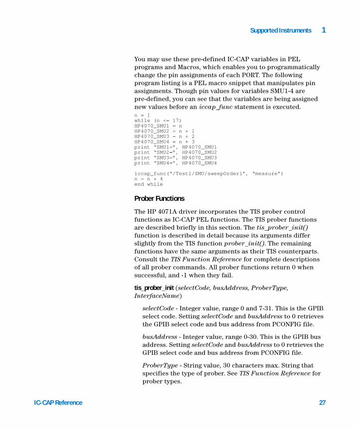
You may use these pre-defined IC-CAP variables in PEL programs and Macros, which enables you to programmatically change the pin assignments of each PORT. The following program listing is a PEL macro snippet that manipulates pin assignments. Though pin values for variables SMU1-4 are pre-defined, you can see that the variables are being assigned new values before an iccap_func statement is executed.n = 1while (n <= 17)HP4070_SMU1 = nHP4070_SMU2 = n + 1HP4070_SMU3 = n + 2HP4070_SMU4 = n + 3print “SMU1=”, HP4070_SMU1print “SMU2=”, HP4070_SMU2print “SMU3=”, HP4070_SMU3print “SMU4=”, HP4070_SMU4
iccap_func(“/Test1/SMU/sweepOrder1”, “measure”)n = n + 4end while
Prober Functions
The HP 4071A driver incorporates the TIS prober control functions as IC-CAP PEL functions. The TIS prober functions are described briefly in this section. The tis_prober_init() function is described in detail because its arguments differ slightly from the TIS function prober_init(). The remaining functions have the same arguments as their TIS counterparts. Consult the TIS Function Reference for complete descriptions of all prober commands. All prober functions return 0 when successful, and -1 when they fail.
tis_prober_init (selectCode, busAddress, ProberType, InterfaceName)
selectCode - Integer value, range 0 and 7-31. This is the GPIB select code. Setting selectCode and busAddress to 0 retrieves the GPIB select code and bus address from PCONFIG file.
busAddress - Integer value, range 0-30. This is the GPIB bus address. Setting selectCode and busAddress to 0 retrieves the GPIB select code and bus address from PCONFIG file.
ProberType - String value, 30 characters max. String that specifies the type of prober. See TIS Function Reference for prober types.
27

28
1 Supported Instruments
InterfaceName - String value. This is the interface name, either TIS_OFFLINE or TIS_ONLINE.
tis_p_home ()
Used for loading a wafer onto the chuck and moving it to the home position.
tis_p_up ()
Moves the chuck of the wafer prober up.
tis_p_down ()
Lowers the chuck of the wafer prober.
tis_p_scale (xIndex, yIndex)
Defines the X & Y stepping dimensions that are used by the tis_p_move and tis_p_imove functions.
tis_p_move (xCoordinate, yCoordinate)
Moves the chuck to an absolute position.
tis_p_imove (xDisplacement, yDisplacement)
Moves the chuck a relative increment from its current position.
tis_p_orig (xCoordinate, yCoordinate)
Defines the current X & Y position of the chuck. Must be called before calling the tis_p_move or tis_p_imove functions.
tis_p_pos (xPosition, yPosition)
Returns the current X & Y position of the chuck.
tis_p_ink (inkCode)
Calls the inker function of the prober if it is supported.
tis_prober_reset ()
Sends a device clear command to the prober.
tis_prober_status (isRemote, onWafer, lastWafer)
IC-CAP Reference

Supported Instruments 1
IC-CAP Reference
Sends a query to the prober to obtain the Remote/Local control state and the edge sensor contact state. The prober should be initialized with tis_prober_init before this function.
tis_prober_get_name (proberModeName)
Sends query to prober to read name of current mode.
tis_prober_get_ba (proberBusAddress)
Sends query to prober to read its bus address.
tis_prober_read_sysconfig (proberType, scba)
Sends query to prober to read its complete interface address including instrument type, select code, and bus address.
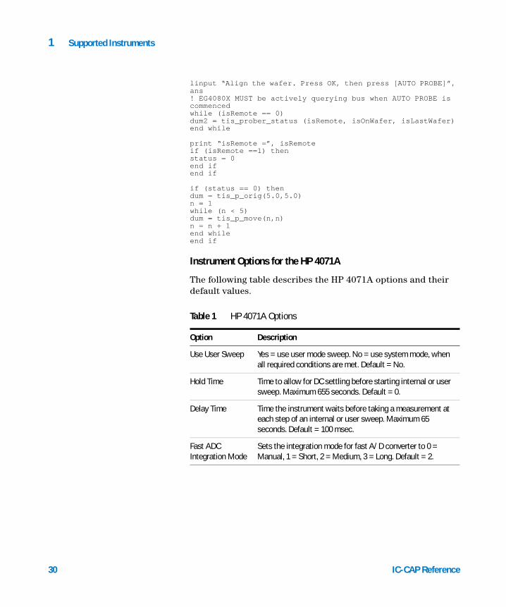
The following PEL macro example uses the prober functions. For the prober used in this example, notice that the operator must manually place the prober into AUTO PROBE mode while the program is actively querying the prober and it is in remote mode. Also notice that isRemote, isOnWafer, and isLastWafer must be parameters that appear in a variable list such as Model Variables.status = -1busAddress = 0selectCode = 0proberType = “EG4080X”interfaceName = “TIS_ONLINE”stepSizeX = 500stepSizeY = 300isRemote = 0isOnWafer = 0isLastWafer = 0dum = 1
! Prober Commands return 0 for success, -1 for failuredum = tis_prober_reset()status=tis_prober_init(selectCode,busAddress,proberType,interfaceName)if (status == 0) thenstatus = tis_p_scale(stepSizeX, stepSizeY)print “status =”, statusend if
if (status == 0) thenstatus = tis_prober_status(isRemote, isOnWafer, isLastWafer)print “status =”, statusprint “isRemote =”, isRemoteend if
if (status == 0) then
29
30
1 Supported Instruments
linput “Align the wafer. Press OK, then press [AUTO PROBE]”, ans! EG4080X MUST be actively querying bus when AUTO PROBE is commencedwhile (isRemote == 0)dum2 = tis_prober_status (isRemote, isOnWafer, isLastWafer)end while
print “isRemote =”, isRemoteif (isRemote ==1) thenstatus = 0end ifend if
if (status == 0) thendum = tis_p_orig(5.0,5.0)n = 1while (n < 5)dum = tis_p_move(n,n)n = n + 1end whileend if
Instrument Options for the HP 4071A
The following table describes the HP 4071A options and their default values.
Table 1 HP 4071A Options
Option Description
Use User Sweep Yes = use user mode sweep. No = use system mode, when all required conditions are met. Default = No.
Hold Time Time to allow for DC settling before starting internal or user sweep. Maximum 655 seconds. Default = 0.
Delay Time Time the instrument waits before taking a measurement at each step of an internal or user sweep. Maximum 65 seconds. Default = 100 msec.
Fast ADC Integration Mode
Sets the integration mode for fast A/D converter to 0 = Manual, 1 = Short, 2 = Medium, 3 = Long. Default = 2.
IC-CAP Reference

Supported Instruments 1
IC-CAP Reference
Fast ADC Integration Value
Sets the integration time in Power Line Cycles (PLC) or number of samples to average for integration. Allowed values depend on setting for Fast ADC Integration Mode:If Integration Mode = 0 or 1, samples = 0, 1 to 4096. Default = 1.If Integration Mode = 2, values are ignored, time is fixed to 1 PLC.If Integration Mode = 3, time = 0, 1 to 100 PLC. Default = 16.If 0 is entered as the value, the default value is used.
Use Smart Fast ADC Integ Mode
Yes/No, default = No. Specifying Yes will use Smart mode integration for fast A/D converter for current measurements. Fast ADC Integ Mode and Fast ADC Integ Value will still be used for voltage measurements.
Smart Fast ADC Integ Value
Sets the integration time in Power Line Cycles (PLC) for integration on current measurements when Use Smart Fast ADC Integ Mode is Yes. Values can be 0, or 1 to 100 PLC. If 0 is entered as the value, the default of 16 PLC will be used.
Slow ADC Integration Mode
Sets the integration mode for high-resolution (slow) A/D converter to 0 = Manual, 1 = Short, 2 = Medium, 3 = Long. Default = 2.
Slow ADC Integration Value
Sets the integration time in Power Line Cycles (PLC) or number of samples to average for integration. Allowed values depend on setting for Slow ADC Integration Mode:If Integration Mode = 0, time = 0, 80E-6 to 20E-3 seconds, or 1 to 100 PLC. Default = 240E-6If Integration Mode = 1, time = 0, 80E-6 to 20E-3 seconds. Default = 480E-6.If Integration Mode = 2, values are ignored, time is fixed to 1 PLC.If Integration Mode = 3, time = 0, 1 to 100 PLC. Default = 16.If 0 is entered as the value, the default value is used.
Slow ADC Auto Zero On
Sets SMU auto zero function to 0 = Off or 1= On. When turned on, the offset error is canceled at each measurement. Default = last valid value.
Table 1 HP 4071A Options (continued)
Option Description
31

32
1 Supported Instruments
Use Smart Slow ADC Integ Mode
Yes/No, default = No. Specifying Yes will use Smart mode integration for high-resolution (slow) A/D converter for current measurements. Slow ADC Integ Mode and Slow ADC Integ Value will still be used for voltage measurements.
Smart Fast ADC Integ Value
Sets the integration time in Power Line Cycles (PLC) for integration on current measurements when Use Smart Slow ADC Integ Mode is Yes. Values can be 0, or 1 to 100 PLC. If 0 is entered as the value, the default of 16 PLC will be used.
Ground Open Guard Terminals
Connects guard terminals of unused measurement pins to circuit common. 0 = Disconnects terminals, any other value connects them.Default = 0.
Pins Sets the PORT that is connected to the test head pins.
Guard Pins Sets the pins to use for guard terminal. Available only for SMU1 and 2.
Fast/Slow ADC Selects ADC. F = high speed (fast), S = high resolution (slow).
Port Filter On Sets the SMU output filter mode, 0 = Off, 1 = On. Higher speed measurement is used when filter is off. Overshoot voltage or current is reduced when filter is on. Default = 0.
V Range(0.0 = Auto)
Sets the SMU voltage range. For MPSMU, allowed range is -100 to 100, with recommended range of 0, 2, 20, 40, 100. For HPSMU, allowed range is -200 to 200, with recommended range of 0, 2, 20, 40, 100, 200.Default = 0 (auto range).
I Range(0.0 = Auto)
Sets the SMU current range. For MPSMU, allowed range is -0.1 to 0.1, with recommended range of 0, 1E-9, 1E-8, 1E-7, 1E-6, 1E-5, 1E-4, 1E-3, 1E-2, 1E-1. For HPSMU, allowed range is -1 to 1, with recommended range of 0, 1E-9, 1E-8, 1E-7, 1E-6, 1E-5, 1E-4, 1E-3, 1E-2, 1E-1, 1.Default = 0 (auto range).
Table 1 HP 4071A Options (continued)
Option Description
IC-CAP Reference

Supported Instruments 1
IC-CAP Reference
Power Compliance
Sets SMU power compliance in Watts. Allowed range for MPSMU is 0, 0.001 to 2. Allowed range for HPSMU is 0, 0.001 to 14.
Pulse Mode On Sets pulse mode. NO = off, YES = on.
Pulse Base Sets level of waveform’s base for pulsed spot measurements. For MPSMU, allowed range is -0.1 to 0.1. For HPSMU, allowed range is -1 to 1. See Figure 1 for pulse waveform characteristics.
Pulse Width Sets width of pulse for pulsed spot measurements. Allowed range is 0.0005 to 2.0000 seconds. Default = 0.005. See Figure 1 for pulse waveform characteristics.
Pulse Period Sets period of pulse for pulsed spot measurements. Allowed range is 0, 0.0050 to 5.0000 seconds. Default = 0.2. See Figure 1 for pulse waveform characteristics.
Perform Cal? TRUE = IC-CAP invokes calibration routine if a calibration is needed.FALSE = IC-CAP does not invoke calibration routine if a calibration is needed.
Cal Type Sets the type of calibration routine to perform. Values are OPEN, SHORT, BOTH. BOTH invokes the OPEN and SHORT calibration routines.
High Pin High voltage pin connection.
Low Pin Low voltage pin connection.
Guard Pins Guard pin connection.
Integ Time Sets the CMU measurement’s integration time. Allowed values are 1 = Short, 2 = Medium, 3 = Long.
Hold Time Sets the sweep hold time for C-G-V measurement by the CMU. Allowed range is 0 to 650.000 seconds. Default = 0.
Delay Time Sets the sweep delay time for C-G-V measurement by the CMU. Allowed range is 0 to 650.000 seconds. Default = 0.
Freq Sets the CMU measurement frequency. Allowed values are 1E+3, 1E+4, 1E+5, 1E+6 Hz.
Table 1 HP 4071A Options (continued)
Option Description
33

34
1 Supported Instruments
The following figure is a diagram of the pulse waveform used in pulsed spot measurements showing Pulse Base, Pulse Width, and Pulse Period.
Signal Level Sets the CMU measurement’s test signal level. Allowed range is 0 to 2.0 volts (standard), and 0 to 20.0 volts (option 001). Default = last valid setting, or 0.03.
High Pins High voltage pin connection.
Low Pins Low voltage pin connection.
Auto Zero On Sets auto zero mode for DVM. 0 = disable, 1 = enable. Default = last valid setting.
Integ Time Sets integration time for DVM. Allowed range is 0, 0.5E-6 to 999999.9E-6 seconds; 1 to 10 PLC and 10 to 100 PLC. If set to 0, integration time is set to default value. Default = 0.5E-6.
Figure 1 Pulse Base, Width, and Period in Pulsed Spot Measurements
Table 1 HP 4071A Options (continued)
Option Description
IC-CAP Reference

Supported Instruments 1
HP 4140 pA Meter/DC Voltage Source
IC-CAP Reference
The HP 4140 is equipped with 2 DC voltage source units and 1 low current measurement unit. The units take measurements in either the internal system or user sweep mode.
IC-CAP assigns the following names to the units:
The HP 4140 driver is an example of a driver created using the Open Measurement Interface. The driver’s source code can be found in the files user_meas2.h and user_meas2.C in the directory $ICCAP_ROOT/src. For information, refer to Chapter 2, “Drivers.”
To recognize which data delimiter (CR/LF or Comma) is used, IC-CAP performs a spot I measurement only when an HP 4140 is first accessed (when the Measure command is issued). When the data delimiter is changed, choose Rebuild in the Hardware Setup window so that IC-CAP will note the change.
With a ramp sweep, measured current I can be translated into quasi-static C by the following equation. Use a transform to perform this calculation.
The following table describes the HP 4140 options and their default values, where applicable.
VA DC Voltage Source Unit. VA supports internal linear sweeps using step or ramp sweep mode. This unit can also be used in user sweep mode.
VB DC Voltage Source Unit. VB only sources a constant voltage. If VB is assigned to the main sweep, user sweep mode is required.
LCU pA Current Monitor Unit.
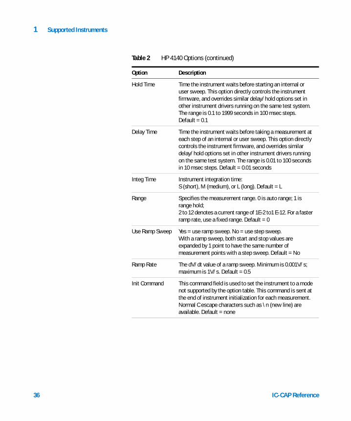
Table 2 HP 4140 Options
Option Description
Use User Sweep Yes = use user sweep.No = use the instrument’s internal sweep. Default = No
CI
RampRate--------------------------- Farads[ ]=
35
36
1 Supported Instruments
Hold Time Time the instrument waits before starting an internal or user sweep. This option directly controls the instrument firmware, and overrides similar delay/hold options set in other instrument drivers running on the same test system. The range is 0.1 to 1999 seconds in 100 msec steps. Default = 0.1
Delay Time Time the instrument waits before taking a measurement at each step of an internal or user sweep. This option directly controls the instrument firmware, and overrides similar delay/hold options set in other instrument drivers running on the same test system. The range is 0.01 to 100 seconds in 10 msec steps. Default = 0.01 seconds
Integ Time Instrument integration time: S (short), M (medium), or L (long). Default = L
Range Specifies the measurement range. 0 is auto range; 1 is range hold; 2 to 12 denotes a current range of 1E-2 to1 E-12. For a faster ramp rate, use a fixed range. Default = 0
Use Ramp Sweep Yes = use ramp sweep. No = use step sweep.With a ramp sweep, both start and stop values are expanded by 1 point to have the same number of measurement points with a step sweep. Default = No
Ramp Rate The dV/dt value of a ramp sweep. Minimum is 0.001V/s; maximum is 1V/s. Default = 0.5
Init Command This command field is used to set the instrument to a mode not supported by the option table. This command is sent at the end of instrument initialization for each measurement. Normal C escape characters such as \n (new line) are available. Default = none
Table 2 HP 4140 Options (continued)
Option Description
IC-CAP Reference
Supported Instruments 1
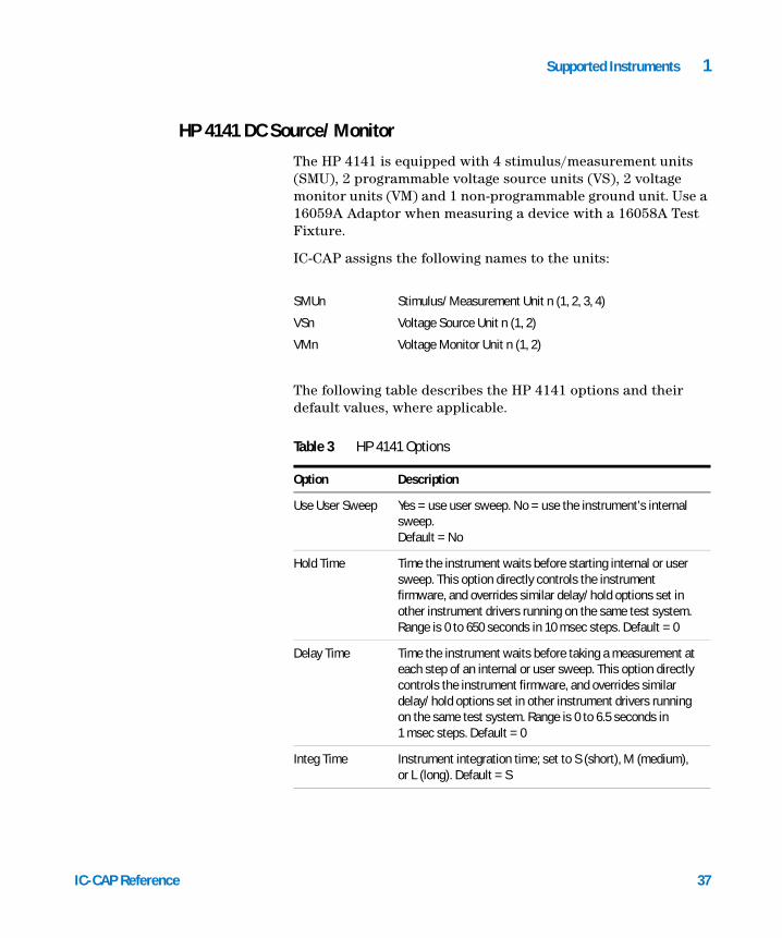
HP 4141 DC Source/Monitor
IC-CAP Reference
The HP 4141 is equipped with 4 stimulus/measurement units (SMU), 2 programmable voltage source units (VS), 2 voltage monitor units (VM) and 1 non-programmable ground unit. Use a 16059A Adaptor when measuring a device with a 16058A Test Fixture.
IC-CAP assigns the following names to the units:
The following table describes the HP 4141 options and their default values, where applicable.
SMUn Stimulus/Measurement Unit n (1, 2, 3, 4)
VSn Voltage Source Unit n (1, 2)
VMn Voltage Monitor Unit n (1, 2)
Table 3 HP 4141 Options
Option Description
Use User Sweep Yes = use user sweep. No = use the instrument’s internal sweep.Default = No
Hold Time Time the instrument waits before starting internal or user sweep. This option directly controls the instrument firmware, and overrides similar delay/hold options set in other instrument drivers running on the same test system. Range is 0 to 650 seconds in 10 msec steps. Default = 0
Delay Time Time the instrument waits before taking a measurement at each step of an internal or user sweep. This option directly controls the instrument firmware, and overrides similar delay/hold options set in other instrument drivers running on the same test system. Range is 0 to 6.5 seconds in 1 msec steps. Default = 0
Integ Time Instrument integration time; set to S (short), M (medium), or L (long). Default = S
37

38
1 Supported Instruments
Init Command Command field to set the instrument to a mode not supported by the option table. This command is sent at the end of instrument initialization for each measurement. Normal C escape characters such as \n (new line) are available. Default = none
Table 3 HP 4141 Options (continued)
Option Description
HP/Agilent 4142 Modular DC Source/Monitor
The 4142 contains 8 configurable plug-in slots for:
• High-power stimulus/measurement units (HPSMU)
• Medium-power stimulus/measurement units (MPSMU)
• High current unit (HCU), high voltage unit (HVU)
• Voltage source units (VS)
• Voltage monitor units (VM)
• Analog Feedback units (AFU—not supported by IC-CAP)
The 4142 ground unit (GND) provides a means for connecting device terminals to a ground reference and can sink current up to 1.6A. This ground unit cannot be programmed or monitored.
Unit names are dependent on the slot they occupy. An SMU (except MPSMU) uses 2 slots in the mainframe; the value of slot number n is the higher of the 2 slots. IC-CAP assigns the following names to the units:
MPSMUn Medium Powered Stimulus/Measurement Unit in slot n
HPSMUn High Powered Stimulus/Measurement Unit in slot n
HCUn High Current Stimulus/Measurement Unit in slot n
HVUn High Voltage Stimulus/Measurement Unit in slot n
VSmn Voltage Source Unit m (1 or 2) in slot n
VMmn Voltage Monitor Unit m (1 or 2) in slot n
IC-CAP Reference

Supported Instruments 1
IC-CAP Reference
The 4142 has a total maximum power consumption of 32W for HPSMU, MPSMU, HCU, HVU and VS/VM. If a measurement is performed and the 32W limit is exceeded, the measurement will not be attempted and IC-CAP will issue an error message. Power consumed by the VS/VM unit (HP/Agilent 41424A) is 2.2W at the 20V range and 0.88W at the 40V range. When using SMUs to source either voltage or current, refer to the Agilent 4142 Operation Manual for the actual SMU power calculations.
NOTE To save power, IC-CAP disconnects output switches of unused HCUs and HVUs when they are not used with the current Setup.
In the user and the internal system mode, voltage and current pulsed measurements are supported. Quasi-pulsed spot measurement is not supported by IC-CAP. For information on how to set up a pulsed measurement, refer to the Pulse entries in Table 5.
HCU and 2-channel pulsed measurements are supported with ROM version 3.0 and later; HVU is supported with version 4.0 and later; Module Selector requires version 4.1.
SMU
Current-forced SMUs of the same type can be connected in parallel to increase the output current. Use SYNC sweep if you want double current at each sweep point. System Sweep can be used for 2 HPSMUs; however, User Sweep must be used for 2 HCUs. To avoid a warning message, set the system variable PARALLEL_INPUT_UNITS_OK to True.
HCU
An HCU can force up to 10A with 10V in the pulse mode only. Its pulse base is fixed to zero and it cannot force a constant value. Both 1- and 2-channel measurements are supported with an HCU.
39

40
1 Supported Instruments
1-Channel Pulse Because an HCU can force only a pulse, an HCU can be used without placing its name in the pulse unit field in the Instrument Options folder. This is called an implicit pulse channel and its pulse width and period are taken from the Instrument Options folder. The pulse base is always set to zero for an implicit pulse channel (HCU). The pulse width and pulse period of an HCU have a different specification from other units. The pulse width must be 0.1 to 1 msec; the pulse period must be 10 to 500 msec; the pulse duty must be 10 percent or less when its output or compliance current is 1A or less, and must be 1 percent or less when its current is more than 1A.
If an HCU is specified as the pulse unit explicitly in the Instrument Options folder, this is called an explicit pulse channel and the pulse base in the Instrument Options folder must be set to zero.
2-Channel Pulse When 2 pulsed channels are used, the primary channel must be an HCU; the secondary channel can be an HCU, SMU, or VS—it cannot be an HVU. For information on the 2-channel configuration, refer to the following table.
HVU
An HVU can force up to 1000V with 10 mA in either the constant or the pulsed mode. This unit has the same specification about the pulse width, pulse period, and pulse duty as other SMUs.
Table 4 2-Channel Options
Channel Primary Secondary
Pulse Unit HCU only HCU/SMU/VS
Pulse Width 0.1 to 0.8 msec; from Instrument Options folder
approximately 1 msec
Pulse Period from Instrument Options folder from Instrument Options folder
Pulse Base 0 only from Instrument Options folder
Declared implicit from Instrument Options folder
IC-CAP Reference

Supported Instruments 1
IC-CAP Reference
An HVU is a unipolar source that requires the output polarity be set before you set its output value. An internal sweep from the minus-to-plus or from the plus-to-minus region is impossible; set the Use User Sweep option to Yes, if such a sweep range is necessary.
To perform the self test and calibration, the INTLK switch must be closed for an HVU. At the start and end of each measurement, IC-CAP instructs all used units to force zero for safety reasons. The shock hazard lamp of the HP/Agilent 16088B test fixture remains on after each measurement because the output switch of the used HVU has been closed to force zero.
VM
A differential voltage measurement of a VM unit is supported by supplying a command string to the Init Command field in the Instrument Options folder. If a VM unit is in slot 8, add the command string “VM 8,2;” to the Init Command field. This sets the VM unit at slot 8 to a differential mode where it measures the differential voltage of VM18 versus VM28. Then add an output for VM18 (not VM28) to the Setup. When simulating this differential mode VM, VM18 should correspond to the + Node to have the same polarity between measurement and simulation.
The following table describes the HP/Agilent 4142 options and their default values, where applicable.
41

42
1 Supported Instruments
Table 5 HP/Agilent 4l42 Options
Option Description
Use User Sweep Yes = use user mode sweep. No = use system mode, when all required conditions are met. Default = No
Hold Time Time to allow for DC settling before starting internal or user sweep. This option directly controls the instrument firmware, and overrides similar delay/hold options set in other instrument drivers running on the same test system. Maximum 655 seconds. Default = 0
Delay Time Time the instrument waits before taking a measurement at each step of an internal or user sweep. This option directly controls the instrument firmware, and overrides similar delay/hold options set in other instrument drivers running on the same test system. Maximum 65 seconds. Default = 100 msec
Integ Time Instrument’s integration time; can be set to S (short), M (medium), or L (long). Default = S
Range Specifies the measurement range. 0 specifies auto range. Applies to all SMUs in this 4142. Refer to the Agilent 4142 Operation Manual for definitions of other ranges. Default = 0
SMU Filters ON Yes = filters ON. No = filters OFF.Applies to all SMUs in this 4142. A pulsed unit is automatically set to filter off. Default = Yes
Pulse Unit Enter name of a pulsed unit when taking pulsed measurements.
Pulse Base Enter value of pulse base.
Pulse Width Enter value of pulse width.
Pulse Period Enter value of pulse period.
Module Control Enter SMU, HCU, or HVU for module selection with option 300. For user relays, enter an exact argument for the ERC command (for example, 2,1,0). When blank, no unit is connected by the module selector. Refer to the 4142 GPIB Command Reference Manual for the ERC command.
IC-CAP Reference

Supported Instruments 1
IC-CAP Reference
† Supported for internal sweep mode only (USE USER SWEEP = NO) and DC only measurement setups.
This option applies to SMUs only. The allowable range of power compliance depends on the sweep source (SMU type) and is not monitored by IC-CAP. Refer to instrument's documentation for more details.
IC-CAP requires rectangular datasets, thus when a power compliance is specified, the instrument concludes the measurement at the power compliance limit, but IC-CAP fills the datasets with the last point measured below power compliance.
Init Command Command field used to set the instrument to a mode not supported by the option table. Command is sent at the end of instrument initialization for each measurement. Normal C escape characters such as \n (new line) are available. Default = none
Power Compliance †
Specify power compliance in Watts with 1mW resolution. Specifying 0 (zero) disables power compliance mode (default).
Table 5 HP/Agilent 4l42 Options (continued)
Option Description
HP 4145 Semiconductor Parameter Analyzer
The HP 4145 is equipped with the following units:
• Four programmable stimulus/measurement units (SMU)
• Two programmable voltage source units (VS)
• Two voltage monitor units (VM)
Time-domain measurement is not supported by IC-CAP.
NOTE A user-defined function may cause an error E07 in the HP 4145 when the function refers to non-existing source names. Clear any user-defined functions in the HP 4145 before making a measurement with IC-CAP.
IC-CAP assigns the following names to the units:
SMUn Stimulus/Measurement Unit n (1, 2, 3, 4)
43

44
1 Supported Instruments
To recognize which data delimiter (CR/LF or Comma) is used, IC-CAP performs a 2-point VM measurement only when an HP 4145 is first accessed (when the Measure command is issued). When the data delimiter is changed, choose Rebuild in the Hardware Setup window so that IC-CAP will note the change.
VSn Voltage Source Unit n (1, 2)
VMn Voltage Monitor Unit n (1, 2)
NOTE The HP 4145 performs an internal logarithmic sweep only if the number of points per decade is 10, 25 or 50; otherwise IC-CAP will force the measurement into User Sweep. If a Setup contains only a single Input with a sweep order of 1, IC-CAP will force the measurement into User Sweep.
HP 4145 requires its test fixture lid be closed in User Sweep mode for safety reasons, even though output is low. A Shorting Connector (P/N 04145-61623) can be used to bypass this lid closure check.
NOTE The HP 4145 offers the internal secondary sweep capability known as VAR2. However, the internal SYNC sweep always depends on the primary sweep source VAR1. When a secondary SYNC sweep is desired, use User Sweep.
NOTE Always fill the Node Name field of each Input in a Setup because the HP 4145 needs a channel name generated from a Node Name. The channel names must be unique within a Setup for the HP 4145 internal sweep mode.
The following table describes the HP 4145 options and their default values, where applicable.
IC-CAP Reference

Supported Instruments 1
IC-CAP Reference
Table 6 HP 4145 Options
Option Description
Use User Sweep Yes = use user sweep. No = use the instrument’s internal sweep. Default = No
Hold Time Time the instrument waits before starting an internal or user sweep. This option directly controls the instrument firmware, and overrides similar delay/hold options set in other instrument drivers running on the same test system. Range is 0 to 650 sec in 10 msec steps. Default = 0
Delay Time Time the instrument waits before taking a measurement at each step of an internal or user sweep. This option directly controls the instrument firmware, and overrides similar delay/hold options set in other instrument drivers running on the same test system. The range is 0 to 6.5 sec in 1 msec steps. Default = 0
Integ Time Instrument integration time; set to S (short), M (medium), or L (long). Default = S
Init Command This command field is used to set the instrument to a mode not supported by the option table. This command is sent at the end of instrument initialization for each measurement. Normal C escape characters such as \n (new line) are available. Default = none
45

1 Supported Instruments
HP/Agilent 4155 Semiconductor Parameter Analyzer
46
The HP/Agilent 4155 is equipped with the following units:
• Four programmable medium power stimulus/measurement units (MPSMU)
• Two programmable voltage source units (VS)
• Two voltage monitor units (VM)
IC-CAP assigns the following names to the units:
The HP 41501A is an optional SMU and pulse generator expander box that can be attached to and controlled by the 4155. The HP 41501A can be equipped with a high power stimulus/measurement unit (HPSMU), medium power stimulus/measurement units (MPSMU), and pulse generator units (PGU) (IC-CAP does not support PGUs). The availability and combination of these units depends on the expander box option.
MPSMUn Medium Power Stimulus/Measurement Unit n (1, 2, 3, 4)
VSUx Voltage Source Unit n (1, 2)
VMUx Voltage Monitor Unit n (1, 2)
NOTE When making pulsed mode measurements, if you specify an SMU as the unit for an Output, and there is no corresponding SMU unit for an Input, compliance errors will result. The same problem occurs if you specify Voltage Monitor units. To prevent this from happening, you should define a compliance value for Output-only SMUs and a measurement range for Voltage Monitor units (VMs) through system variables, as follows, using the unit name:
HRSMUx_COMP HPSMUx_COMP MPSMUx_COMPwhere x = 1, 2, 3, 4, 5, 6
VMU1_RANGE_VALUE VMU2_RANGE_VALUE
IC-CAP assigns the following names to the units of the optional HP 41501A:
IC-CAP Reference

Supported Instruments 1
IC-CAP Reference
• MPSMUn Medium Power Stimulus/Measurement Unit n (5, 6)
• HPSMU5 High Power Stimulus/Measurement Unit
A ground unit (GNDU) provides a means for connecting device terminals to a ground reference and can sink up to 1.6A. The ground unit is supported by IC-CAP but will not appear in the Hardware Editor Configuration dialog box. For information on how to use the ground unit, refer to the section “Adding a Ground Unit" in the User’s Guide.
In both the user and internal sweep mode, voltage and current pulsed measurements are supported. Only the SMUs can be specified as pulse units because the PGUs are not currently supported. For information on how to set up a pulsed measurement, refer to the Pulse options in Table 7.
NOTE The HP/Agilent 4155 offers the internal secondary sweep capability known as VAR2. However, the internal SYNC sweep always depends on the primary sweep source VAR1. When a secondary SYNC sweep is desired, use User Sweep.
NOTE To execute a user sweep measurement, IC-CAP sets the HP/Agilent 4155 to the Sampling mode with the number of samples equal to 1. The front panel screen activity is turned off at the start of the measurement and is turned back on after the measurement is completed.
Although the 4155 performs an internal logarithmic sweep if the number of points per decade is 10, 25 or 50, IC-CAP will force the measurement into the User Sweep for all specified logarithmic sweeps. If a Setup specification contains a single Input with a sweep order of 1, IC-CAP will force the measurement into User Sweep.
The following table describes the 4155 options and their default values, where applicable.
47

48
1 Supported Instruments
Notes:† Supported for internal sweep mode only (USE USER SWEEP = NO) and DC only measurement setups.
Table 7 HP/Agilent 4155 (and HP/Agilent 4156) Option
Option Description
Use User Sweep Yes = use user mode sweep. No = use system mode, when required conditions are met. Default = No
Hold Time Time delay before starting an internal or user sweep to allow for DC settling. This option directly controls the instrument firmware, and overrides similar delay/hold options set in other instrument drivers running on the same test system. Maximum is 655 seconds. Default = 0
Delay Time Time the instrument waits before taking a measurement at each step of an internal or user sweep. This option directly controls the instrument firmware, and overrides similar delay/hold options set in other instrument drivers running on the same test system. This value is not used for pulsed sweeps. Maximum is 65 seconds. Default = 0
Delay for Timeouts
For long-running measurements (that use a high number of averages, for example) use this option to avoid measurement timeouts. Default=0
Integ Time Instrument integration time; set to S (short), M (medium), or L (long). Default = S
Pulse Unit Enter the name of a pulsed unit when taking pulsed measurements.
Pulse Base Enter the value of the pulse base.
Pulse Width Enter the value of the pulse width.
Pulse Period Enter the value of the pulse period.
Init Command Command field to set the instrument to a mode not supported by the option table. This command is sent at the end of instrument initialization for each measurement. Normal C escape characters such as \n (new line) are available. Default = none
Power Compliance †
Specify power compliance in Watts with 1mW resolution. Specifying 0 (zero) disables power compliance mode (default).
IC-CAP Reference

Supported Instruments 1
IC-CAP Reference
This option applies to SMUs only. The allowable range of power compliance depends on the sweep source (SMU type) and is not monitored by IC-CAP. Refer to instrument's documentation for more details.
IC-CAP requires rectangular datasets, thus when a power compliance is specified, the instrument concludes the measurement at the power compliance limit, but IC-CAP fills the datasets with the last point measured below power compliance.
HP/Agilent 4156 Precision Semiconductor Parameter Analyzer
The HP/Agilent 4156 is equipped with the following units:
• Four programmable high-resolution stimulus/measurement units (HRSMU)
• Two programmable voltage source units (VS)
• Two voltage monitor units (VM)
This instrument is designed for Kelvin connections and is capable of low- resistance and low-current measurements.
IC-CAP assigns the following names to the units:
The HP 41501A is an optional SMU and pulse generator expander box that can be attached to and controlled by the 4156. The HP 41501A can be equipped with the following units:
• High-power stimulus/measurement unit (HPSMU)
• Medium power stimulus/measurement units (MPSMU)
• Pulse generator units (PGU—not supported by IC-CAP)
IC-CAP assigns the following names to the units of the optional HP 41501A:
HRSMUn High Resolution Stimulus/Measurement Unit n (1, 2, 3, 4)
VSUx Voltage Source Unit n (1, 2)
VMUx Voltage Monitor Unit n (1, 2)
MPSMUn Medium Power Stimulus/Measurement Unit n (5, 6)
HPSMU5 High Power Stimulus/Measurement Unit
49

50
1 Supported Instruments
A ground unit (GNDU) provides a means for connecting device terminals to a ground reference and can sink up to 1.6A. The ground unit is supported by IC-CAP but will not appear in the Hardware Editor Configuration dialog box. For information on how to use the ground unit, refer to the section “Adding a Ground Unit" in the User’s Guide.
In both the user and internal sweep mode, voltage and current pulsed measurements are supported. Only the SMUs can be specified as pulse units because PGUs are not currently supported. For information on how to set up a pulsed measurement, refer to the Pulse options in Table 7.
NOTE The HP/Agilent 4156 offers the internal secondary sweep capability known as VAR2. However, the internal SYNC sweep always depends on the primary sweep source VAR1. When a secondary SYNC sweep is desired, use User Sweep.
NOTE To execute a user sweep measurement, IC-CAP sets the HP/Agilent 4156 to the Sampling mode with the number of samples equal to 1. The front panel screen activity is turned off at the start of the measurement and is turned back on after the measurement is completed.
NOTE Although the HP/Agilent 4156 performs an internal logarithmic sweep if the number of points per decade is 10, 25 or 50, IC-CAP will force the measurement into the user sweep for all specified logarithmic sweeps. If a Setup specification contains a single Input with a sweep order of 1, IC-CAP forces the measurement into user sweep.
Options for the HP 4156 are the same as for the HP 4155; refer to Table 7.
Agilent E5260 Series Parametric Measurement Solutions
Agilent E5260 Series High Speed Measurement Solutions are built around the following:
• E5260A 8-slot parametric measurement mainframe
IC-CAP Reference

Supported Instruments 1
IC-CAP Reference
• E5262A/3A 2-channel source/monitor units
Available Source/Monitor Units (SMUs):
• E5290A High Power source/monitor unit (HPSMU)
• E5291A Medium Power source/monitor unit (MPSMU)
The E5260A 8-slot parametric measurement mainframe holds up to 8 single-slot modules, such as a medium power source/monitor unit (MPSMU), or up to 4 dual-slot modules, such as a high power source/monitor unit (HPSMU).
The E5262A 2-channel source/monitor unit contains 2 medium power source/monitor units (SMUs).
The E5263A 2-channel source/monitor unit contains 1 high power and 1 medium power SMU.
If you install 4 HPSMUs into the E5260A mainframe, you can output 1 Amp of current from each of these units simultaneously.
The E5260A/B mainframe's ground unit (GNDU) provides a means for connecting device terminals to a ground reference. The GNDU will sink 4 amps of current without having to worry about any resistive ground rise issues. This ground unit cannot be programmed or monitored.
Unit names are dependent on the slot they occupy. A high power SMU occupies 2 slots in the mainframe, a medium or a high resolution SMU occupies 1 slot; the value of slot number n is the higher of the 2 slots. IC-CAP assigns the following names to the units:
The E5260A 8-slot parametric measurement mainframe has a total maximum power consumption of 80W for all plug-in modules. The total maximum power consumption limits for the E5262A and E5263A are 8W and 24W respectively. If a
MPSMUn Medium Powered Stimulus/Measurement Unit in slot n
HPSMUn High Powered Stimulus/Measurement Unit in slot n
51

52
1 Supported Instruments
measurement is performed and the power limitation is exceeded, the measurement will not be attempted and IC-CAP will issue an error message.
HPSMU
The high power source monitor units will provide up to 50 milliamps of current at ±200 volts and 1 amp of current at ±40 volts. Up to 4 HPSMUs can be used at one time in the E5260A mainframe. See manual for complete measurement and force ranges specifications such as resolution and measurement accuracy.
MPSMU
The medium power source monitor units will provide up to 20 milliamps of current at ±200 volts and 200 milliamps of current at ±20 volts. Up to 8 MPSMUs can be used at one time in the E5260A. See manual for complete measurement and force ranges specifications such as resolution and measurement accuracy.
Instrument Options
The following table describes the Agilent E5260A options and their default values, where applicable.
Table 8 Agilent E5260A Options
Option Description
Use User Sweep Yes = use user mode sweep. No = use internal sweep, when all required conditions are met. Default = No
Hold Time Time to allow for DC settling before starting internal or user sweep. This option directly controls the instrument firmware, and overrides similar delay/hold options set in other instrument drivers running on the same test system. Maximum 655 seconds. Default = 0
IC-CAP Reference

Supported Instruments 1
IC-CAP Reference
Delay Time Time the instrument waits before taking a measurement at each step of an internal or user sweep. This option directly controls the instrument firmware, and overrides similar delay/hold options set in other instrument drivers running on the same test system. Maximum 65 seconds. Default = 100 msec
Integ Time Instrument’s integration time; can be set to S (short), M (medium), or L (long). Default = S
Power Compliance †
Specify power compliance in Watts with 1mW resolution. Specifying 0 (zero) disables power compliance mode (default).
SMU Filters ON Yes = filters ON, No = filters OFF.Applies to all SMUs in this E5260. Default = No
Range Manager Mode
Specify Range Manager mode: 1, 2, or 3. 1 = deactivate Range Manager (default)2 = set Range Manager to mode 23 = set Range Manager to mode 3The Range Manager command is used to avoid potential voltage spikes during current range switching when using autorange. See Instrument Programming Guide††† under RM command for details.
Range Manager Setting
Set the rate of the Range Manager command.Allowed values are between 11 and 100.This option is only active when Range Manager Mode is set to 2 or 3.
Enable <SMU name> Range Manager
Enables Range Manager at the setting values entered above for the named SMU. Default = No.
Table 8 Agilent E5260A Options (continued)
Option Description
53

54
1 Supported Instruments
<SMU name> In/Out Range
Specify force (Input Sweep) and Output measurement ranges. Default is autorange (0 or 0/0) for both Input and Output measurement ranges.When an SMU is used in an IC-CAP input definition to force voltage or current, a specific force range may be selected. The force resolution†† will depend on the selected range. When an SMU is used in an IC-CAP output definition to monitor voltage or current, a specific measurement range may be selected. The measurement resolution will depend on the selected range. Both fixed (negative range number) and limited auto (positive numbers) ranges are supported. Allowed ranges are SMU dependent and are forced by IC-CAP during initial measurement setup. See instrument manual††† for allowed values for each SMU. When instrument supports 2 values for setting the same range, IC-CAP only supports the smaller of the 2. For example, to select a 20 V range, the manual suggests using 12 or 200. Use the value 12, to select that range.Ranges must be in the format ForceRange/OutRange, e.g., 13/15 for a voltage SMU monitoring current means Force Voltage Range=13 (40 V, 2mV resolution), Output Current Measurement Range=15 (10 uA limited autorange).
Pulse Unit Enter name of a pulsed unit when taking pulsed measurements.
Pulse Base Enter value of pulse base.
Pulse Width Enter value of pulse width.
Pulse Period Enter value of pulse period.
Disable Self-Cal Controls the status of the E5260A self-calibration routine during measurements. Yes = self-cal disabled. No= self-cal enabled. Default = No.
Output I/O Port (ERC Command)
Send the user string with the ERC command
Output I/O Port (ERM Command)
Send the user string with the ERM command
Delay for timeouts Sets the delay before a measurement attempt times out.
Table 8 Agilent E5260A Options (continued)
Option Description
IC-CAP Reference

Supported Instruments 1
IC-CAP Reference
† Supported for internal sweep mode only (USE USER SWEEP = NO) and DC only measurement setups.
The allowable range of power compliance depends on the sweep source (SMU type) and is not monitored by IC-CAP. Refer to instrument's documentation for more details.
IC-CAP requires rectangular datasets, thus when a power compliance is specified, the instrument concludes the measurement at the power compliance limit, but IC-CAP fills the datasets with the last point measured below power compliance.†† Agilent E5260A, E5262A, E5263A Technical Overview—see Medium and High Power SMUs technical specifications.††† Agilent E5260A series Programming Guide—Chapter 4 “Command Reference”—Section “Command Parameters”
Init Command Command field used to set the instrument to a mode not supported by the option table. Command is sent at the end of instrument initialization for each measurement. Normal C escape characters such as \n (new line) are available. Default = none
Table 8 Agilent E5260A Options (continued)
Option Description
Agilent E5270 Series Parametric Measurement Solutions
Agilent E5270 Series Parametric Measurement Solutions are built around the following:
• E5270A 8-slot parametric measurement mainframe (obsolete)
• E5270B 8-slot parametric measurement mainframe
• E5272A/3A 2-channel source/monitor units (obsolete)
Available Source/Monitor Units (SMUs):
• E5280A High Power source/monitor unit (HPSMU) for E5270A only
• E5280B High Power source/monitor unit (HPSMU) for E5270B only
• E5281A Medium Power source/monitor unit (MPSMU) for E5270A only
• E5281B Medium Power source/monitor unit (MPSMU) for E5270B only
55

56
1 Supported Instruments
• E5287A High Resolution source/monitor unit (HRSMU) for E5270B only
The E5270A 8-slot parametric measurement mainframe holds up to 8 single-slot modules, such as a medium power source/monitor unit (MPSMU), or up to 4 dual-slot modules, such as a high power source/monitor unit (HPSMU).
The E5270B 8-slot parametric measurement mainframe holds up to 8 single-slot modules, such as a medium power source/monitor unit (MPSMU, HRSMU), or up to 4 dual-slot modules, such as a high power source/monitor unit (HPSMU).
The E5272A 2-channel source/monitor unit contains 2 medium power source/monitor units (SMUs).
The E5273A 2-channel source/monitor unit contains 1 high power and 1 medium power SMU.
If you install 4 HPSMUs into E5270A/B mainframes, you can output 1 Amp of current from each of these units simultaneously.
The E5270A/B mainframe's ground unit (GNDU) provides a means for connecting device terminals to a ground reference. The GNDU will sink 4 amps of current without having to worry about any resistive ground rise issues. This ground unit cannot be programmed or monitored.
Unit names are dependent on the slot they occupy. A high power SMU occupies 2 slots in the mainframe, a medium or a high resolution occupies 1 slot; the value of slot number n is the higher of the 2 slots. IC-CAP assigns the following names to the units:
The E5270A and E5270B 8-slot parametric measurement mainframes have a total maximum power consumption of 80W for all plug-in modules. The total maximum power consumption
MPSMUn Medium Powered Stimulus/Measurement Unit in slot n
HPSMUn High Powered Stimulus/Measurement Unit in slot n
HRSMUn High Resolution Source/Monitor Unit in slot n (E5270B only)
IC-CAP Reference

Supported Instruments 1
IC-CAP Reference
limits for the E5272A and E5273A are 8W and 24W respectively. If a measurement is performed and the power limitation is exceeded, the measurement will not be attempted and IC-CAP will issue an error message.
HPSMU
The high power source monitor units will provide up to 50 milliamps of current at ±200 volts and 1 amp of current at ±40 volts. Up to 4 HPSMUs can be used at one time in the E5270A mainframe. Since SMUs characteristic may vary with version, see manual for complete measurement and force ranges specifications such as resolution and measurement accuracy.
MPSMU
The medium power source monitor units will provide up to 20 milliamps of current at ±100 volts and 100 milliamps of current at ±20 volts (200 mA for the E5281A). Up to 8 MPSMUs can be used at one time in the E5270A and E5270B mainframes. Since SMUs characteristic may vary with version, see manual for complete measurement and force ranges specifications such as resolution and measurement accuracy.
HRSMU
The medium power/high resolution source monitor units provide up to 20 milliamps of current at ±100 volts and 100 milliamps of current at ±20 volts. Up to 8 HRSMUs can be used at one time in the E5270B mainframe. In the lowest current range, 10 pA, HRSMU's current force resolution can be as low as 5 fA with a measurement resolution as low as 1 fA.
Instrument Options
The following table describes the Agilent E5270A/B options and their default values, where applicable.
57
58
1 Supported Instruments
Table 9 Agilent E5270A/B Options
Option Description
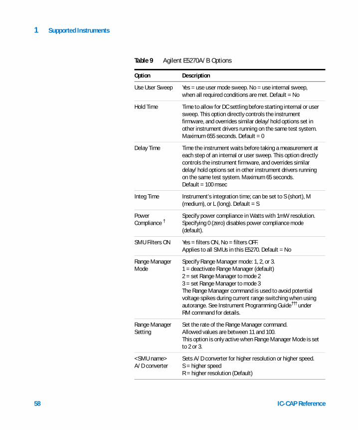
Use User Sweep Yes = use user mode sweep. No = use internal sweep, when all required conditions are met. Default = No
Hold Time Time to allow for DC settling before starting internal or user sweep. This option directly controls the instrument firmware, and overrides similar delay/hold options set in other instrument drivers running on the same test system. Maximum 655 seconds. Default = 0
Delay Time Time the instrument waits before taking a measurement at each step of an internal or user sweep. This option directly controls the instrument firmware, and overrides similar delay/hold options set in other instrument drivers running on the same test system. Maximum 65 seconds. Default = 100 msec
Integ Time Instrument’s integration time; can be set to S (short), M (medium), or L (long). Default = S
Power Compliance †
Specify power compliance in Watts with 1mW resolution. Specifying 0 (zero) disables power compliance mode (default).
SMU Filters ON Yes = filters ON, No = filters OFF.Applies to all SMUs in this E5270. Default = No
Range Manager Mode
Specify Range Manager mode: 1, 2, or 3. 1 = deactivate Range Manager (default)2 = set Range Manager to mode 23 = set Range Manager to mode 3The Range Manager command is used to avoid potential voltage spikes during current range switching when using autorange. See Instrument Programming Guide††† under RM command for details.
Range Manager Setting
Set the rate of the Range Manager command. Allowed values are between 11 and 100.This option is only active when Range Manager Mode is set to 2 or 3.
<SMU name> A/D converter
Sets A/D converter for higher resolution or higher speed.S = higher speedR = higher resolution (Default)
IC-CAP Reference

Supported Instruments 1
IC-CAP Reference
Enable <SMU name> Range Manager
Enables Range Manager at the setting values entered above for the named SMU. Default = No.
<SMU name> In/Out Range
Specify force (Input Sweep) and Output measurement ranges. Default is autorange (0 or 0/0) for both Input and Output measurement ranges.When an SMU is used in an IC-CAP input definition to force voltage or current, a specific force range may be selected. The force resolution†† will depend on the selected range. When an SMU is used in an IC-CAP output definition to monitor voltage or current, a specific measurement range may be selected. The measurement resolution will depend on the selected range. Both fixed (negative range number) and limited auto (positive numbers) ranges are supported. Allowed ranges are SMU dependent and are forced by IC-CAP during initial measurement setup. See instrument manual††† for allowed values for each SMU. When instrument supports 2 values for setting the same range, IC-CAP only supports the smaller of the 2. For example, to select a 20 V range, the manual suggests using 12 or 200. Use the value 12, to select that range.Ranges must be in the format ForceRange/OutRange, e.g., 13/15 for a voltage SMU monitoring current means Force Voltage Range=13 (40 V, 2mV resolution), Output Current Measurement Range=15 (10 uA limited autorange).
Pulse Unit Enter name of a pulsed unit when taking pulsed measurements.
Pulse Base Enter value of pulse base.
Pulse Width Enter value of pulse width.
Pulse Period Enter value of pulse period.
Disable Self-Cal Controls the status of the E5270A self-calibration routine during measurements. Yes = self-cal disabled. No= self-cal enabled. Default = No.
Output I/O Port (ERC Command)
Send the user string with the ERC command
Table 9 Agilent E5270A/B Options (continued)
Option Description
59

60
1 Supported Instruments
† Supported for internal sweep mode only (USE USER SWEEP = NO) and DC only measurement setups.
The allowable range of power compliance depends on the sweep source (SMU type) and is not monitored by IC-CAP. Refer to instrument's documentation for more details.
IC-CAP requires rectangular datasets, thus when a power compliance is specified, the instrument concludes the measurement at the power compliance limit, but IC-CAP fills the datasets with the last point measured below power compliance.†† Agilent E5270A, E5272A, E5273A Technical Overview—see Medium and High Power SMUs technical specifications.††† Agilent E5270A series Programming Guide—Chapter 4 “Command Reference”—Section “Command Parameters”
Output I/O Port (ERM Command)
Send the user string with the ERM command
Delay for timeouts Sets the delay before a measurement attempt times out.
Init Command Command field used to set the instrument to a mode not supported by the option table. Command is sent at the end of instrument initialization for each measurement. Normal C escape characters such as \n (new line) are available. Default = none
Table 9 Agilent E5270A/B Options (continued)
Option Description
IC-CAP Reference

Supported Instruments 1
Agilent B1500A Semiconductor Device Analyzer
IC-CAP Reference
The Agilent B1500A Semiconductor Device Analyzer is a modular instrument with a ten-slot configuration that supports both IV and CV measurements.
The B1500A driver supports the following plug-in modules:
• B1510A High Power Source Monitor Unit Module (HPSMU) for B1500
• B1511A Medium Power Source Monitor Unit Module (MPSMU) for B1500
• B1517A High Resolution Source Monitor Unit Module (HRSMU) for B1500
The B1500A driver does NOT support the following plug-in modules:
• B1520A Multi-Frequency Capacitance Measurement Unit Module for B1500 (combined DC-CV measurements not supported)
• E5288A Auto Sense and Switch Unit for B1500
HPSMU
The high power source monitor units will provide up to 1 amp of current at ±200 volts. Up to 4 HPSMUs can be used at one time in the B1500A. Since SMUs characteristic may vary with version, see manual for complete measurement and force ranges specifications such as resolution and measurement accuracy.
MPSMU
The medium power source monitor units will provide up to 100 milliamps of current at ±100 volts. Up to 10 MPSMUs can be used at one time in the B1500A. Since SMUs characteristic may vary with version, see manual for complete measurement and force ranges specifications such as resolution and measurement accuracy.
61

62
1 Supported Instruments
HRSMU
The medium power/high resolution source monitor units provide up to 100 milliamps of current at ±100 volts. Up to 10 HRSMUs can be used at one time in the B1500A. Since SMUs characteristic may vary with version, see manual for complete measurement and force ranges specifications such as resolution and measurement accuracy.
Instrument Options
The following table describes the Agilent B1500A options and their default values, where applicable.
Table 10 Agilent B1500A Options
Option Description
Use User Sweep Yes = use user mode sweep. No = use internal sweep, when all required conditions are met. Default = No
Hold Time Time to allow for DC settling before starting internal or user sweep. This option directly controls the instrument firmware, and overrides similar delay/hold options set in other instrument drivers running on the same test system. Maximum 655 seconds. Default = 0
Delay Time Time the instrument waits before taking a measurement at each step of an internal or user sweep. This option directly controls the instrument firmware, and overrides similar delay/hold options set in other instrument drivers running on the same test system. Maximum 65 seconds. Default = 100 msec
Integ Time Instrument’s integration time; can be set to S (short), M (medium), or L (long). Default = S
Power Compliance †
Specify power compliance in Watts with 1mW resolution. Specifying 0 (zero) disables power compliance mode (default).
SMU Filters ON Yes = filters ON, No = filters OFF.Applies to all SMUs in this E5270. Default = No
IC-CAP Reference

Supported Instruments 1
IC-CAP Reference
Range Manager Mode
Specify Range Manager mode: 1, 2, or 3. 1 = deactivate Range Manager (default)2 = set Range Manager to mode 23 = set Range Manager to mode 3The Range Manager command is used to avoid potential voltage spikes during current range switching when using autorange. See Instrument Programming Guide††† under RM command for details.
Range Manager Setting
Set the rate of the Range Manager command. Allowed values are between 11 and 100.This option is only active when Range Manager Mode is set to 2 or 3.
<SMU name> A/D converter
Sets A/D converter for higher resolution or higher speed.S = higher speedR = higher resolution (Default)
Enable <SMU name> Range Manager
Enables Range Manager at the setting values entered above for the named SMU. Default = No.
Table 10 Agilent B1500A Options (continued)
Option Description
63

64
1 Supported Instruments
<SMU name> In/Out Range
Specify force (Input Sweep) and Output measurement ranges. Default is autorange (0 or 0/0) for both Input and Output measurement ranges.When an SMU is used in an IC-CAP input definition to force voltage or current, a specific force range may be selected. The force resolution†† will depend on the selected range. When an SMU is used in an IC-CAP output definition to monitor voltage or current, a specific measurement range may be selected. The measurement resolution will depend on the selected range. Both fixed (negative range number) and limited auto (positive numbers) ranges are supported. Allowed ranges are SMU dependent and are forced by IC-CAP during initial measurement setup. See instrument manual††† for allowed values for each SMU. When instrument supports 2 values for setting the same range, IC-CAP only supports the smaller of the 2. For example, to select a 20 V range, the manual suggests using 12 or 200. Use the value 12, to select that range.Ranges must be in the format ForceRange/OutRange, e.g., 13/15 for a voltage SMU monitoring current means Force Voltage Range=13 (40 V, 2mV resolution), Output Current Measurement Range=15 (10 uA limited autorange).
Pulse Unit Enter name of a pulsed unit when taking pulsed measurements.
Pulse Base Enter value of pulse base.
Pulse Width Enter value of pulse width.
Pulse Period Enter value of pulse period.
Disable Self-Cal Controls the status of the E5270A self-calibration routine during measurements. Yes = self-cal disabled. No= self-cal enabled. Default = No.
Output I/O Port (ERC Command)
Send the user string with the ERC command
Output I/O Port (ERM Command)
Send the user string with the ERM command
Delay for timeouts Sets the delay before a measurement attempt times out.
Table 10 Agilent B1500A Options (continued)
Option Description
IC-CAP Reference

Supported Instruments 1
IC-CAP Reference
† Supported for internal sweep mode only (USE USER SWEEP = NO) and DC only measurement setups.
The allowable range of power compliance depends on the sweep source (SMU type) and is not monitored by IC-CAP. Refer to instrument's documentation for more details.
IC-CAP requires rectangular datasets, thus when a power compliance is specified, the instrument concludes the measurement at the power compliance limit, but IC-CAP fills the datasets with the last point measured below power compliance.†† Agilent B1500A Technical Overview—see Medium and High Power SMUs technical specifications.††† Agilent B1500A series Programming Guide—Chapter 4 “Command Reference”—Section “Command Parameters”
Configuring the B1500A for IC-CAP Remote Contol
1 Turn on the B1500.
2 Login into Windows but do not start the EasyExpert software.
3 Start the Agilent_Connection_Expert:
Select Start > Programs > Agilent_IO_Library_Suites > Agilent_Connection_Expert.
4 Select GPIB0 > Change_Properties, then uncheck the following checkboxes:
• System_Controller
• Auto-Discover_Instruments_Connected_To_The_Interface
Select OK and exit the dialog.
5 Reboot the B1500A when prompted.
6 Start the EasyExpert software:
Select Start > Start_EasyExpert.
Init Command Command field used to set the instrument to a mode not supported by the option table. Command is sent at the end of instrument initialization for each measurement. Normal C escape characters such as \n (new line) are available. Default = none
Table 10 Agilent B1500A Options (continued)
Option Description
65

66
1 Supported Instruments
Do not press the B1500A Start button, but leave the B1500A Start button on the screen.
NOTE Fully starting the EasyExpert application would prevent IC-CAP from controlling the B1500A.
7 Connect the B1500A instrument to the IC-CAP computer via GPIB interface.
8 From IC-CAP, rebuild the active instrument list:
Select Tools > Hardware Setup > Rebuild.
9 After rebuild is completed, check that the B1500A is in the Active Instrument List.
10 Select the instrument and configure its SMU names according to the names used in your measurement setups.
IC-CAP Reference

Supported Instruments 1
Capacitance-Voltage Meters
IC-CAP Reference
Capacitance-voltage meters supported by IC-CAP are:
• HP 4194 Impedance Analyzer
• HP 4271 1 MHz Digital Capacitance Meter
• HP 4275 Multi-Frequency LCR Meter
• HP 4280 1 MHz Capacitance Meter
• HP/Agilent 4284 Precision LCR Meter
• HP/Agilent 4285 Precision LCR Meter
• Agilent E4980A Precision LCR Meter
• Agilent 4294A Precision Impedance Analyzer
• Agilent E4991A RF Impedance/Material Analyzer
For all capacitance-voltage meters, issue the Calibrate command before starting a measurement, otherwise calibration is carried out automatically at the start of the measurement.
This option directly controls the instrument firmware, and overrides similar delay/hold options set in other instruments’ drivers running on the same test system.
Defining the Reset State
Using the prepare_CV_meter.mdl example model file, you can easily define the reset state for the following instruments:
• HP/Agilent 4284
• HP/Agilent 4285
• Agilent E4980
The IC-CAP drivers reset instruments to known states prior to configuring them for the current measurement. For the 4284, 4285 and E4980, it sends the *RST command, which resets the instruments to a known factory state. However, this default state (1V, 1KHz signal) may cause damage to certain devices between the time the $RST is requested and the time the requested signal level is set.
67

68
1 Supported Instruments
To avoid this problem, you can set the variable LCR_RST_MEM or LCR_RST_MEM_<unit> (e.g., LCR_RST_MEM_CM). The 4284, 4285, and E4980A instruments will use the value of this variable to set the instrument state. For example, if set to 1, the driver will recall instrument state 1 instead of *RST.
Using the prepare_CV_meter.mdl example model file, you can programatically set any state to be the *RST state with a zero signal level. It will also set the variable for you such that when a measurement is performed, this programatically set state is recalled instead of sending *RST.
To prepare a memory location, open and Auto Execute model_files/misc/prepare_CV_meter.mdl, then enter the 3 values below and click OK.
1 Name the unit associated with your instrument.
2 Identify the memory location (0-9 recommended, but you can use any number from 0-19 that your instrument supports.)
3 Indicate if you want the unit number to apply to any 4284, 4284, or E4980A, or only to those with the specified unit name. This selection essentially chooses between setting LCR_RST_MEM or LCR_RST_MEM_<unit>.
HP 4194 Impedance Analyzer
The HP 4194 offers 2 measurement types: impedance analysis and gain-phase measurement. These occupy different test connectors on the test set. IC-CAP supports the impedance analysis type, offering capacitance-voltage and conductance-versus-voltage measurements.
The frequency range is 100 Hz to 40 MHz; to extend this to 100 MHz use the impedance probe kit. An internal DC bias unit can deliver biases between −40V and +40V. An internal oscillator can deliver between 10 mV and 1V rms.
The HP 4194 driver is an example of a driver created using the Open Measurement Interface. The driver source code can be found in the files user_meas.hxx and user_meas.cxx in the directory $ICCAP_ROOT/src. For information, refer to Chapter 2, “Drivers.”
IC-CAP Reference

Supported Instruments 1
IC-CAP Reference
IC-CAP assigns the following name to the unit:
CM Capacitance Meter Unit
NOTE The short calibration of the HP 4194 driver is disabled by default because the CV measurement rarely needs this compensation. However, the SHORT_CAL4194 system variable may be defined and set to Yes to enable the short calibration.
NOTE After a CV measurement is finished, you may notice that a DC bias light on the HP 4194 stays on. This indicates that a bias voltage is still being applied to the test setup. However, the IC-CAP driver sets the DC sweep mode’s bias voltage for the measurement so the DC bias is set to 0 V when the sweep starts and stops.
There are 2 ways you can verify the bias voltage is set to zero. One way is to measure the test setup with a DMM. Another way is to enable IC-CAP’s Screen Debug (Tools > Options > Screen Debug) and see that the following commands are being sent to the CV meter:
START=0.0;STOP=0.0;NOP=2;MANUAL=0.0;OSC=0.01SWM3;TRGM2TRIG
The following table describes the HP 4194 options and their default values, where applicable.
Table 11 HP 4194 Options
Option Description
Use User Sweep Yes = use user sweep. No = use the instrument’s internal sweep.Default = No
Hold Time Time the instrument waits before starting an internal or user sweep. Default = 0
69

70
1 Supported Instruments
Delay Time Time delay, in seconds, the instrument waits before taking a measurement at each step of an internal or user sweep. When biasing the device with an external DC source (e.g., an Agilent 4142B or 4156C), the DC source’s delay/hold options override this option. Default = 0
Meas Freq Oscillator frequency range 100 Hz to 40 MHz. The 41941A/B impedance probe kit extends this to 100 MHz. If the CV_FREQ system variable is defined, it must be set equal to this frequency, otherwise an error is reported. Default = 1 MHz
Integ Time Instrument integration time: S (short), M (medium), or L (long). Default = S
Osc Level Test signal level. Allowable voltage levels and resolutions are: Minimum = 10 mV; Maximum = 1V. Default = 10mV
Averages Number of averages. Maximum = 256. Default = 1
Delay for Timeouts
For long-running measurements (that use a high number of averages, for example) use this option to avoid measurement timeouts. Default=0
Init Command Command field to set the instrument to a mode not supported by the option table. This command is sent at the end of instrument initialization for each measurement. Normal C escape characters such as \n (new line) are available. Default = none
Table 11 HP 4194 Options (continued)
Option Description
HP 4271 1 MHz Digital Capacitance Meter
IC-CAP supports only external bias sources when performing measurements using the HP 4271. Both hardware and software calibrations are available. The instrument makes measurements in user sweep only. If the CV_FREQ system variable is defined, it must be set equal to 1 MHz before making a measurement with the HP 4271, otherwise an error is reported.
IC-CAP Reference

Supported Instruments 1
IC-CAP Reference
IC-CAP assigns the following name to this unit:
CM Capacitance Meter Unit
The following table describes the HP 4271 options and their default values, where applicable.
Table 12 HP 4271 Options
Option Description
Hold Time Time the instrument waits before starting an internal or user sweep. Default = 0
Delay Time Time, in seconds, the instrument waits before taking a measurement at each step of an internal or user sweep. When biasing the device with an external DC source (e.g., an Agilent 4142B or 4156C), the DC source’s delay/hold options override this option. Default = 0
Init Command This is a command field to set the instrument to a mode not supported by the option table. This command is sent at the end of instrument initialization for each measurement. Normal C escape characters such as \n (new line) are available. Default = none
HP 4275 Multi-Frequency LCR Meter
The HP 4275 includes an optional internal DC bias source. IC-CAP checks for this internal bias source when you issue the Rebuild command in the Hardware Setup window. For the internal DC bias to be recognized, the DC BIAS selector switch must be set to Internal. Only hardware calibration is available and the instrument makes measurements in user sweep only.
IC-CAP assigns the following name to this unit:
CM Capacitance Meter Unit
The test signal level on the HP 4275 can only be set manually with the OSC LEVEL dial and MULTIPLIER switches. This signal level must be set by the user to a reasonable value such as 10 mV to obtain accurate results, since a high signal level can
71

72
1 Supported Instruments
modulate the DC operating point. The MULTIPLIER is set to 1 when the instrument is powered up; a different setting must be selected manually.
When using the internal DC bias, the bias unit is also included in the CM unit. Therefore, the unit name of this CM unit should also be entered in the Unit fields of both the voltage bias Input and the capacitance Output specifications of the Setup.
The following table describes the HP 4275 options and their default values, where applicable.
Table 13 HP 4275 Options
Option Description
Hold Time Time the instrument waits before starting an internal or user sweep. Range is 0 to 650 seconds in 10 msec steps. Default = 0
Delay Time Time the instrument waits before taking a measurement at each step of an internal or user sweep. Range is 3 msec to 650 sec. Resolution is in 1 msec steps for the 3 to 65 msec range; 10 msec for the 65.01 to 99.99 msec range; and, 100 msec for the 100 msec to 650 sec range. When biasing the device with an external DC source (e.g., an Agilent 4142B or 4156C), the DC source’s delay/hold options override this option.Default = 3 msec
Meas Freq Measurement Frequencies. When the instrument is not equipped with option 004, it accepts frequency measurements at 10K, 20K, 40K, 100K, 200K, 400K, 1M, 2M, 4M, and 10M. When equipped with option 004, it accepts measurements at 10K, 30K, 50K, 100K, 300K, 500K, 1M, 3M, 5M, and 10M. Enter valid frequencies only. If the CV_FREQ system variable is defined, it must be set equal to this frequency, otherwise an error is reported. Because the unit of CV_FREQ is Hz, divide it by 1K for this field. Default = 1 MHz
High Res Enables or disables high resolution mode. Yes = enabled; No = disabled. Default = No
IC-CAP Reference

Supported Instruments 1
IC-CAP Reference
Init Command Command field to set the instrument to a mode not supported by the option table. This command is sent at the end of instrument initialization for each measurement. Normal C escape characters such as \n (new line) are available. Default = none
Table 13 HP 4275 Options (continued)
Option Description
HP 4280 1 MHz Capacitance Meter
The HP 4280 measures the capacitance-voltage characteristics of semiconductor devices. The test signal of the instrument is a 1 MHz sine wave. The HP 4280 also contains a built-in DC bias source with an output capability of 0 to ±100V and a maximum setting resolution of 1 mV. Capacitance-voltage measurements can be taken using this internal voltage source or an external bias unit. The HP 4280 includes an internal calibration capability. Measurements can be made in either internal or user sweep. If the CV_FREQ system variable is defined, it must be set to 1 MHz before making a measurement with the HP 4280, otherwise an error is reported.
IC-CAP assigns the following name to this unit:
CM Capacitance Meter Unit
When using the internal DC bias, this bias unit is also included in the CM unit. Therefore, the unit name of this CM unit should also be entered in the Unit fields of both the voltage bias Input and the capacitance Output specifications of the Setup.
The following table describes the HP 4280 options and their default values, where applicable.
Table 14 HP 4280 Options
Option Description
Use User Sweep Yes = use user sweep. No = use the instrument’s internal sweep. Default = No
73

74
1 Supported Instruments
Hold Time Time the instrument waits before starting internal or user sweep. Range is 0 to 650 seconds in 10 msec steps. Default = 3 msec
Delay Time Time delay before each measurement is taken when using internal sweep. Range is 3 msec to 650 seconds. Resolution is in 1 msec steps for the 3 to 65 msec range, 10 msec for the 65.01 to 99.99 msec range, and 100 msec for the 100 msec to 650 second range. When biasing the device with an external DC source (e.g., an Agilent 4142B or 4156C), the DC source’s delay/hold options override this option.Default = 3 msec
Delay for Timeouts
For long-running measurements (that use a high number of averages, for example) use this option to avoid measurement timeouts. Default=0
Meas Speed Measuring speed: S (slow), M (medium), or F (fast). Default = S
Sig Level (10, 30) Signal level: 10 or 30 mV rms. Default = 10
High Res Enables or disables high resolution mode. Yes = enabled. No = disabled. Default = No
Conn Mode Connection mode. When using the HP 4280 internal bias source, set to 10. When using an external bias source, connect the source to the EXT-SLOW connector on the HP 4280 rear panel and set the connection mode to 12. Default = 10
Init Command Command field to set the instrument to a mode not supported by the option table. This command is sent at the end of instrument initialization for each measurement. Normal C escape characters such as \n (new line) are available. Default = none
Table 14 HP 4280 Options (continued)
Option Description
IC-CAP Reference

Supported Instruments 1
HP/Agilent 4284 Precision LCR Meter
IC-CAP Reference
The HP/Agilent 4284 is a general purpose LCR meter with a frequency range of 20 Hz to 1 MHz. The instrument includes an internal calibration. Options 001 and 006 are supported by IC-CAP. Option 001 includes a built-in internal bias source. Standard cable lengths are 0 and 1 meter; option 006 supports 2 and 4 meter lengths as well. Measurements can be made in user sweep mode only.
IC-CAP assigns the following name to this unit:
CM Capacitance Meter Unit
When using the internal DC bias, the bias unit is also included in the CM unit. Therefore, the unit name of this CM unit should also be entered in the Unit fields of both the voltage bias Input and the capacitance Output specifications of the Setup.
CAUTION Prior to configuring the HP/Agilent 4284 for the current measurement, the IC-CAP driver resets the 4284 to a known state by sending the *RST command. The default reset state (1V, 1KHz signal) may cause damage to certain devices between the time the $RST is requested and the time the requested signal level is set. To avoid this problem, you can define the reset state. See “Defining the Reset State” on page 67.
The following table describes the HP/Agilent 4284 options and their default values, where applicable.
Table 15 HP/Agilent 4284 Options
Option Description
Hold Time Time the instrument waits before starting an internal or user sweep. Range is 0 to 650 seconds in 10 msec steps. Default = 0
75

76
1 Supported Instruments
Delay Time Time the instrument waits before each sweep point is measured. The range is 0 to 60 seconds. When biasing the device with an external DC source (e.g., an Agilent 4142B or 4156C), the DC source’s delay/hold options override this option.Default = 0
Meas Freq Measuring frequency. Only a set of frequencies are available. The range is 20 Hz to 1 MHz. If the CV_FREQ system variable is defined, it must be set equal to this frequency, otherwise an error is reported. Default = 1 MHz
Integ Time Instrument integration time: S (short), M (medium), or L (long). Default = M
Osc Level Test signal level in volts or amps. Allowable voltage levels and resolutions are:Minimum = 5 mVMaximum = 20V with opt 001, 2V otherwiseBetween 5 mV and 200 mV: resolution = 1 mVBetween 200 mV and 2V: resolution = 10 mVBetween 2V and 20V: resolution = 100 mV (Opt. 001 only)Allowable current levels and resolutions are:Minimum level = 50 µA rmsMaximum level = 200 mA rms with opt 001, 20 mA otherwiseBetween 50 µA and 2 mA: resolution = 10 µABetween 2 mA and 20 mA: resolution = 100 µABetween 20 mA and 200 mA: resolution = 1 mA (Opt. 001 only)
The Instrument Options folder accepts test signal levels outside these ranges. However, if a measurement is attempted, an error message is issued and the measurement is not performed. Default = 10m
Osc Mode [V,I] Specify V (voltage) or I (current). Automatic Level Control (ALC) is not supported. Default = V
Table 15 HP/Agilent 4284 Options (continued)
Option Description
IC-CAP Reference

Supported Instruments 1
IC-CAP Reference
Averaging[1-256]
The averaging rate of the instrument. Default = 1
Cable Length Cable length, in meters: 0, 1, 2, or 4. Default = 1M
Delay for Timeouts
For long-running measurements (that use a high number of averages, for example) use this option to avoid measurement timeouts. Default=0
Init Command Command field to set the instrument to a mode not supported by the option table. This command is sent at the end of instrument initialization for each measurement. Normal C escape characters such as \n (new line) are available. Default = none
Table 15 HP/Agilent 4284 Options (continued)
Option Description
HP/Agilent 4285 Precision LCR Meter
The HP/Agilent 4285 is a general purpose LCR meter with a frequency range of 75 kHz to 30 MHz. The instrument includes an internal calibration. Option 001, which adds a built-in internal bias source, is supported by IC-CAP. Measurements can be made in user sweep only.
IC-CAP assigns the following name to this unit:
CM Capacitance Meter Unit
When using the internal DC bias, the bias unit is also included in the CM unit. Therefore, the unit name of this CM unit should also be entered in the Unit fields of both the voltage bias Input and the capacitance Output specifications of the Setup.
CAUTION Prior to configuring the HP/Agilent 4285 for the current measurement, the IC-CAP driver resets the 4285 to a known state by sending the *RST command. The default reset state (1V, 1KHz signal) may cause damage to certain devices between the time the $RST is requested and the time the requested signal level is set. To avoid this problem, you can define the reset state. See “Defining the Reset State” on page 67.
77

78
1 Supported Instruments
The following table describes the HP/Agilent 4285 options and their default values, where applicable.
Table 16 HP/Agilent 4285 Options
Option Description
Hold Time Time the instrument waits before starting an internal or user sweep. Default = 0
Delay Time Time the instrument waits before each sweep point is measured. Range is 0 to 60 seconds in 1 msec steps. When biasing the device with an external DC source (e.g., an Agilent 4142B or 4156C), the DC source’s delay/hold options override this option.Default = 0
Meas Freq Measuring frequency. Range is 75 kHz to 30 MHz with 100 Hz resolution. If the CV_FREQ system variable is defined, it must be set equal to this frequency, otherwise an error is reported. Default = 1 MHz
Integ Time Instrument integration time: S (short), M (medium), or L (long). Default = M
Osc Level Test signal level in volts or amps. The allowable voltage levels and resolutions are:Minimum level = 5 mV rmsMaximum level = 2V rmsBetween 5 mV and 200 mV: resolution = 1 mVBetween 200 mV and 2V: resolution = 10 mV
The allowable current levels and resolutions are:Minimum level = 200 µA rmsMaximum level = 20 mA rmsBetween 200 µA and 2 mA: resolution = 20 µABetween 2 mA and 20 mA: resolution = 200 µA
The Instrument Options folder accepts test signal levels outside these ranges. However, if a measurement is attempted, an error message is issued and the measurement is not performed.Default = 10m
IC-CAP Reference

Supported Instruments 1
IC-CAP Reference
Osc Mode [V,I] Specify V (voltage) or I (current). Automatic Level Control (ALC) is not supported. Default = V
Averaging[1-256]
The averaging rate of the instrument. Default = 1
Cable Length Cable length, in meters: 0, 1, or 2. Default = 1
Delay for Timeouts
For long-running measurements (that use a high number of averages, for example) use this option to avoid measurement timeouts. Default=0
Init Command Command field to set the instrument to a mode not supported by the option table. This command is sent at the end of instrument initialization for each measurement. Normal C escape characters such as \n (new line) are available. Default = none
Table 16 HP/Agilent 4285 Options (continued)
Option Description
Agilent E4980A Precision LCR MeterThe Agilent E4980A is a general-purpose LCR meter. The Agilent E4980A is used for evaluating LCR components, materials, and semiconductor devices over a wide range of frequencies (20 Hz to 20 MHz) and test signal levels (0.1 mVrms to 2 Vrms, 50 µA to 20 mArms). With Option 001, the E4980A’s test signal level range spans 0.1 mV to 20 Vrms, and 50 µA to 200 mArms. Also, the E4980A with Option 001 enables up to ±40 Vrms DC bias measurements (without Option 001, up to ±2 Vrms), DCR measurements, and DC source measurements using the internal voltage source.
IC-CAP assigns the following name to this unit:
CM Capacitance Meter Unit
When using the internal DC bias, the bias unit is also included in the CM unit. Therefore, the unit name of this CM unit should also be entered in the Unit fields of both the voltage bias Input and the capacitance Output specifications of the Setup.
79

1 Supported Instruments
CAUTION Prior to configuring the Agilent E4980A for the current measurement, the IC-CAP driver resets the E4980 to a known state by sending the *RST command. The default reset state (1V, 1KHz signal) may cause damage to certain devices between the time the $RST is requested and the time the requested signal level is set. To avoid this problem, you can define the reset state. See “Defining the Reset State” on page 67.
80
The following table describes the Agilent E4980A options and their default values, where applicable.
Table 17 Agilent E4980A Options
Option Description
Hold Time Time the instrument waits before starting an internal or user sweep. Range is 0 to 650 seconds in 10 msec steps.Default = 0
Delay Time Time the instrument waits before each sweep point is measured. The range is 0 to 60 seconds. When biasing the device with an external DC source (e.g., an Agilent 4142B or 4156C), the DC source’s delay/hold options override this option.Default = 0
Meas Freq Measuring frequency. Only a set of frequencies are available. The range is 20 Hz to 1 MHz. If the CV_FREQ system variable is defined, it must be set equal to this frequency, otherwise an error is reported. Default = 1 MHz
Integ Time Instrument integration time: S (short), M (medium), or L (long). Default = M
IC-CAP Reference

Supported Instruments 1
IC-CAP Reference
Osc Level Test signal level in volts or amps. Allowable voltage levels and resolutions are:Minimum = 0 mVrmsMaximum = 20 Vrms with opt 001, 2Vrms otherwiseBetween 0 mVrms and 200 mVrms: resolution = 100 µVrmsBetween 200 mVrms and 500 mVrms:
resolution = 200 µVrmsBetween 500mVrms and 1Vrms: resolution = 500 µVrmsBetween 1 Vrms and 2 Vrms: resolution = 1 mVrmsBetween 2 Vrms and 5 Vrms: resolution = 2 mVrms
(Opt. 001 only)Between 5 Vrms and 10 Vrms: resolution = 5 mVrms
(Opt. 001 only)Between 10 Vrms and 20 Vrms†: resolution = 10 mVrms
(Opt. 001 only)† When the test frequency is more than 1 MHz, the
maximum oscillator voltage level that can be set is15 Vrms.
Allowable current levels and resolutions are:Minimum level = 0 ArmsMaximum level = 100 mArms with opt 001, 20 mA
otherwiseBetween 0 µArms and 2 mArms: resolution = 1 µArmsBetween 2 mArms and 5 mArms: resolution = 2 µArmsBetween 5 mArms and 10 mArms: resolution = 5 µArms Between 10 µArms and 20 mArms: resolution = 10 µArmsBetween 20 mArms and 50 mArms: resolution = 20 µArms
(Opt. 001 only)Between 50 mArms and 100 mArms:
resolution = 50 µArms (Opt. 001 only)
The Instrument Options folder accepts test signal levels outside these ranges. However, if a measurement is attempted, an error message is issued and the measurement is not performed. Default = 10m
Osc Mode [V,I] Specify V (voltage) or I (current). Automatic Level Control (ALC) is not supported. Default = V
Table 17 Agilent E4980A Options (continued)
Option Description
81

82
1 Supported Instruments
Averaging[1-256]
The averaging rate of the instrument. Default = 1
Cable Length Cable length, in meters: 0, 1, 2, or 4. Default = 1M
Delay for Timeouts
For long-running measurements (that use a high number of averages, for example) use this option to avoid measurement timeouts. Default=0
Init Command Command field to set the instrument to a mode not supported by the option table. This command is sent at the end of instrument initialization for each measurement. Normal C escape characters such as \n (new line) are available. Default = none
Table 17 Agilent E4980A Options (continued)
Option Description
Agilent 4294A Precision Impedance Analyzer
The Agilent 4294A is a precision impedance analyzer designed to measure impedance (inductance, capacitance, and resistance) at frequencies between 40 Hz and 110 MHz. The instrument includes an internal calibration.
IC-CAP assigns the following name to this unit:
CM Capacitance Meter Unit
When using the internal DC bias, the bias unit is also included in the CM unit. Therefore, the unit name of this CM unit should also be entered in the Unit fields of both the voltage bias Input and the capacitance Output specifications of the Setup.
Frequency cannot be swept using IC-CAP.
The following table describes the Agilent 4294A options and their default values, where applicable.
IC-CAP Reference

Supported Instruments 1
IC-CAP Reference
Table 18 Agilent 4294A Options
Option Description
Use User Sweep Yes = use user sweep. No = use the instrument’s internal sweep. Default = No.
Hold Time Time the instrument waits before starting an internal or user sweep. Default = 0.
Delay Time Time the instrument waits before each sweep point is measured. Range is 0 to 30 seconds. Resolution is 1 msec. Default = 0.
Meas Freq Measuring frequency. Only a set of frequencies are available. Range is 40 Hz to 110 MHz. Resolution is 1 mHz at 40 Hz and 1 kHz at 110 MHz. If the CV_FREQ system variable is defined, it must be set equal to this frequency, otherwise an error is reported. Default = 1 MHz.
Bandwidth Measurement bandwidth. 1 FAST (fastest measurement), 2, 3, 4, 5 PRECISE (highest accuracy measurement). Default = 1.
Osc Level Test signal level. Allowable voltage levels and resolutions are: minimum = 5 mV, maximum = 1 V. Default = 500 mV. Resolution = 1 mV.
Averages [1-256] Point Averages, minimum 1, maximum = 256. Default = 1
Delay for Timeouts
For long-running measurements (that use a high number of averages, for example) use this option to avoid measurement timeouts. Default=0.
Meas Range Selects DC bias range. Three ranges: 1 mA, 10 mA, and 100 mA. Default = 1 mA.
Init Command Command field to set the instrument to a mode not supported by the option table. This command is sent at the end of instrument initialization for each measurement. Normal C escape characters such as \n (new line) are available. Default = no entry.
83

1 Supported Instruments
Agilent E4991A RF Impedance/Material Analyzer
84
The Agilent E4991A is an RF impedance/material analyzer designed to measure impedance (inductance, capacitance, and resistance) at frequencies between 1 MHz and 3 GHz. Measurements can be made in internal sweep mode only.
IC-CAP assigns the following name to this unit:
CM Capacitance Meter Unit
When using the internal DC bias, the bias unit is also included in the CM unit. Therefore, the unit name of this CM unit should also be entered in the Unit fields of both the voltage bias Input and the capacitance Output specifications of the Setup.
Frequency cannot be swept using IC-CAP.
The following table describes the Agilent E4991A options and their default values, where applicable.
Table 19 Agilent E4991A Options
Option Description
Use User Sweep Yes = use user sweep, No = use the instrument’s internal sweep, default = No.
Hold Time Time the instrument waits before starting an internal or user sweep, default = 0.
Delay Time Time the instrument waits before each sweep point is measured. Range is 0 to 20 seconds, default = 0.
Meas Freq Measuring frequency. Only a set of frequencies are available. Range is 1 MHz to 3 GHz with 1 kHz resolution. If the CV_FREQ system variable is defined, it must be set equal to this frequency, otherwise an error is reported, default = 1 MHz.
Osc Level Test signal level in volts. Allowable voltage levels and resolutions are: minimum = 5 mV; maximum = 502 mV, default = 100 mV, resolution = 1 mV. The Instrument Options dialog accepts test signal levels outside these ranges. However, if a measurement is attempted, an error message is issued and the measurement is not performed.
IC-CAP Reference
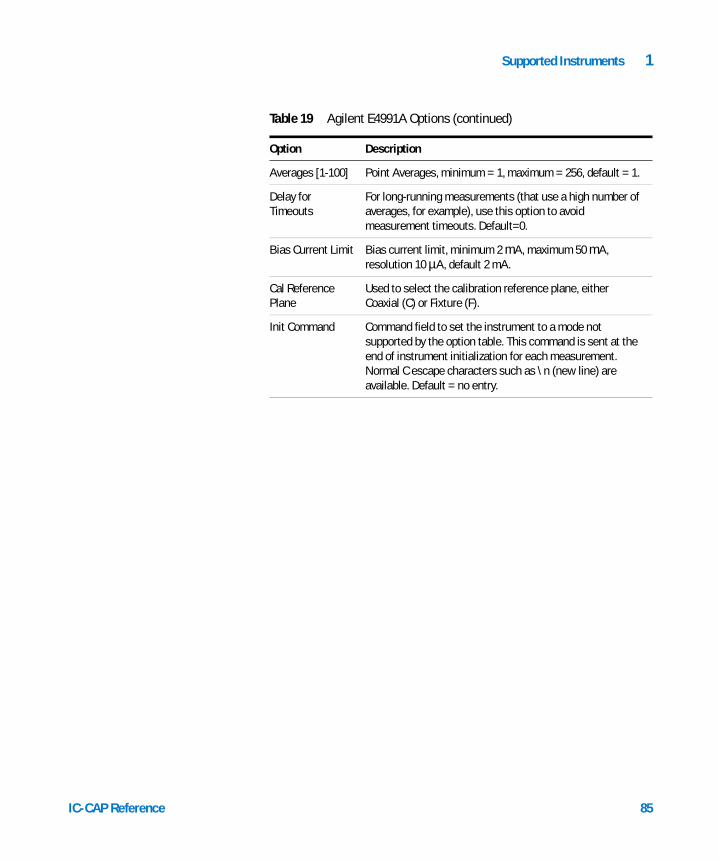
Supported Instruments 1
IC-CAP Reference
Averages [1-100] Point Averages, minimum = 1, maximum = 256, default = 1.
Delay for Timeouts
For long-running measurements (that use a high number of averages, for example), use this option to avoid measurement timeouts. Default=0.
Bias Current Limit Bias current limit, minimum 2 mA, maximum 50 mA, resolution 10 µA, default 2 mA.
Cal Reference Plane
Used to select the calibration reference plane, either Coaxial (C) or Fixture (F).
Init Command Command field to set the instrument to a mode not supported by the option table. This command is sent at the end of instrument initialization for each measurement. Normal C escape characters such as \n (new line) are available. Default = no entry.
Table 19 Agilent E4991A Options (continued)
Option Description
85

1 Supported Instruments
Network Analyzers
86
A network analyzer is an integrated stimulus/response test system that measures the magnitude and phase characteristics of a 1-port or multi-port network by comparing the incident signal with the signal transmitted through the device or reflected from its inputs. A network analyzer provides a waveform with a specified attenuation and frequency as inputs to the network or device under test. It then measures the magnitude and the phase information of both the reflected and transmitted waves.
The network analyzers supported by IC-CAP are:
• Agilent E5071C ENA Series Network Analyzer
• Agilent PNA Series Vector Network Analyzer
• HP 3577 Network Analyzer
• HP/Agilent 8510 Network Analyzer
• HP/Agilent 8702 Network Analyzer
• HP/Agilent 8719 Network Analyzer
• HP/Agilent 8720 Network Analyzer
• HP/Agilent 8722 Network Analyzer
• HP/Agilent 8753 Network Analyzer
• Wiltron360 Network Analyzer
A network analyzer contains an S-parameter test set that allows automatic selection of S11, S21, S12, and S22 measurements. S-parameters are used to quantify the signals involved in microwave design. S, for scattering, describes the act of an energy wave front entering, exiting, or reflecting off the 2-port network being characterized. Physically, the wave is an electromagnetic flow of energy, a traveling complex voltage wave. Mathematically, the S-parameter is a voltage normalized by the impedance of the environment so that its expression relates all information about voltage, current, and impedance at the same time.
IC-CAP Reference

Supported Instruments 1
IC-CAP Reference
The primary advantage of characterization with S-parameters is that they can be measured by terminating a network in its characteristic impedance instead of a short or open. The following figure mathematically illustrates how S-parameters are defined.
Referring to the previous figure, when a network port is terminated so that there is no reflected energy, it is said to be terminated in its characteristic impedance Z0. If at port 2, a2 = 0 because b2 looked into a Z0 load and was not reflected, then
b1 = S11 • a1+S12 • 0 or
This defines an input reflection coefficient with the output terminated by a matched load (Z0). Similarly,
defines an output reflection coefficient with the input terminated by Z0.
Figure 2 Mathematical Description of S-parameters
S11
b1a1------=
a2 0=
S22
b2a2------=
a1 0=
87

88
1 Supported Instruments
defines the forward transmission (insertion) gain with the output port terminated in Z0.
defines the reverse transmission (insertion) gain with the input port terminated in Z0.
The following figure is a graphic description of how S-parameters are defined.
S21
b2a1------=
a2 0=
S12
b1a2------=
a1 0=
IC-CAP Reference

Supported Instruments 1
IC-CAP Reference
Figure 3 Graphic Description of S-parameters
The smaller S11, the less energy is reflected (better source match.
S21 is gain. Usually, the larger the better.
The smaller S22, the less energy is reflected (better load match.
The smaller S12, the more isolation the source has from the load.
89

1 Supported Instruments
Agilent E5071C ENA Series Network AnalyzerNOTE The error terms saved to file during a network analyzer software calibration are not identified by error code.
The order shown below represents the order in which they are saved and displayed in IC-CAP:
0. EDF [directivity] 1. EDR [directivity] 2. EXF [isolation] 3. EXR [isolation] 4. ESF [source match] 5. ERF [ref freq response] 6. ESR [source match] 7. ERR [ref freq response] 8. ELF [load match] 9. ETF [trans freq response] 10. ELR [load match] 11. ETR [trans freq response]
90
IC-CAP supports the Agilent E5071C ENA Series RF network analyzer. The following table lists each analyzer and its frequency range:
IC-CAP assigns the following name to this unit:
NWA Network Analyzer Unit
Table 20 Supported ENA Series Network Analyzers
Instrument Name Low Frequency High Frequency
Agilent E5071C-240/440 9 kHz 4.5 GHz
Agilent E5071C-245/445 100 kHz 4.5 GHz
Agilent E5071C-280/480 9 kHz 8.5 GHz
Agilent E5071C-285/485 100 kHz 8.5 GHz
IC-CAP Reference

Supported Instruments 1
NOTE IC-CAP loads the Instrument Options parameters, including Source Power, Sweep Time, and so on, during an ENA measurement. Since this involves setting values critical to the calibration, an error or warning may be issued.
IC-CAP Reference
The ENA Series network analyzers are recognized when you issue the Rebuild, Measure, or Calibrate command.
This driver only supports Frequency mode with sweep types of Linear, List, Log, and Constant.
• Linear sweep mode allows you to specify the start/stop frequencies, number of points, and step size.
• List sweep mode allows you to sweep up to 202 individual frequencies.
• Log sweep mode allows you to specify start/stop frequencies, number of decades, and points per decade. The points are log spaced and you can specify a total of 202 points.
• Constant mode allows you to measure 1 individual frequency.
Table 21 on page 92 describes the E5071C ENA options and their default values, where applicable. For more information on options, refer to the E5071C ENA Series Network Analyzer Help file located in the analyzer.
A self-test function is not provided for this instrument.
Calibration
The IC-CAP Calibrate command loads Setup information into the ENA prior to calibrating. When running a measurement afterwards, the calibration set must match IC-CAP's Setup and it must be valid.
Only hardware calibration is supported. The calibration must be either manually executed or executed using dedicated calibration software and saved in a directory in the ENA. The calibration and state file must have extension .sta. To measure calibrated data, set the instrument option Cal Type to H (Hardware) and specify a file name with a .sta extension in the Instrument Option field Cal/State File Name.
91

92
1 Supported Instruments
On the ENA mainframe, the default directory for saving and reading calibration and state files is D:\State. You can save the calibration file in a different directory and still recall it from IC-CAP by setting the system variable ENA_CAL_FILE_PATH to the new directory (use full path such us D:\my_dir\).
When running a measurement recalling a calibration set, the frequency sweep and the instrument options should be consistent with the calibration set. Warnings will be issued in the IC-CAP Status window when relevant ENA measurement settings (such as IF Bandwidth or Port Power) differ from the calibration settings.
NOTE The .sta file type should be a save state file that includes the instrument state and the calibration data. So when saving the .sta file inside the instrument for further use, make sure to use the State & Cal save type in the Save/Recall menu.
The ENA has the capability to interpolate between points. Therefore, you can specify a different frequency range and number of points during a measurement as long as the measured frequency range is within the calibrated frequency range. However, be aware that a loss in accuracy occurs due to interpolation.
Table 21 Agilent E5071C ENA Options
Option Description
Use User Sweep [Yes/No]
Yes = use user sweep. No = use instrument's internal sweep.Default = No
Hold Time (sec) Time, in seconds, the instrument waits before each sweep to allow for DC settling.Default = 0
Delay Time (sec) Time the instrument waits before setting each frequency in user sweep mode.Default = 0
Sweep Time (sec) Time the instrument takes for each sweep. 0 = AutoDefault = 0
IC-CAP Reference

Supported Instruments 1
IC-CAP Reference
Sweep Type [SA] S = Stepped mode. A = Analog (ramp) modeDefault = S
Port Power Coupled [Yes/No]
Yes = Coupled mode. No = Non-Coupled mode.Default = Yes.When ports are coupled, the Port1 Src Power value is used for both Port 1 and 2. Port2 Src Power is ignored.
Port1 Src Power (dBm)
Defines the source Power for Port 1 and 2 when ports are coupled or the source power for Port 1 when ports are uncoupled. The power range depends on the ENA model and options.
Port2 Src Power (dBm)
Defines the source power for Port 2 when ports are uncoupled. This option field is ignored when ports are coupled. The power range depends on the ENA model and options.
Power Slope (db/GHz)
Can be any value between −2 and +2 dB/GHzDefault = 0
IF Bandwidth (Hz) Range 10 Hz to 500 kHzNominal settings are: 10, 15, 20, 30, 40, 50, 70, 100, 150, 200, 300, 400, 500, 700, 1k, 1.5k, 2k, 3k, 4k, 5k, 7k, 10k, 15k, 20k, 30k, 40k, 50k, 70k, 100k, 150k, 200k, 300k, 400k, 500kHzDefault = 1000 HzNote: If a invalid value is specified, the ENA will not round it to the nearest available value. It will round up to the next higher value.
Avg Factor [1-1024]
Number of averages per measurement. [1-1024]Default = 1
Cal Type [HN] H = Hardware calibration. N = No calibrationDefault = N
Cal/State File Name [ .sta only]
Name of .sta file (with stored calibration and instrument state) to be used.Default = none
Table 21 Agilent E5071C ENA Options (continued)
Option Description
93

94
1 Supported Instruments
Technical Notes
• You can perform averaging by increasing the number of averages or decreasing the IF filter bandwidth. Both methods result in more samples taken at each frequency point. Decreasing the IF filter bandwidth not only increases the number of samples but also the time at each frequency point resulting in a longer sweep time. Increasing the number of averages, increases the number of sweeps. Although the driver supports both modes, using IF bandwidth for averaging is generally more efficient.
Use ENA Calibration Settings [Yes/No]
This setting can be set to Yes only if a calibration file is available and Calibration Type is set to H (Hardware).Default = NoWhen set to Yes, IC-CAP loads the calibration and runs the measurement without further initializing the instrument (i.e. without downloading the current Instrument Table settings). Although IC-CAP uses the calibration settings for measurements, it still sets the sweep settings (e.g. Start, Stop, Sweep Type, etc.). Therefore, make sure the requested sweep setting is consistent with the calibration settings as IC-CAP attempts to run the measurement without performing any frequency range checking. Also note that when this option is set to Yes, the driver responds as if MEASURE_FAST=Yes (i.e., calibration is loaded only when the measurement is first run or after errors or warnings occur).
Delay for timeouts (sec)
For long-running measurements (that use a high number of averages, for example) use this option to avoid measurement timeouts.Default = 0
Init Command Command field to set the instrument to a mode not supported by the option table. Command is sent at the end of instrument initialization for each measurement. Normal C escape characters such as \n (new line) are available.Default = none
Table 21 Agilent E5071C ENA Options (continued)
Option Description
IC-CAP Reference

Supported Instruments 1
IC-CAP Reference
• Coupled ports have the same source power connected to Port 1 and Port 2 for forward and reverse S-parameter measurements.
• If you have significant insertion loss due to cables or bias networks, use power slope. Using the appropriate power slope can compensate for insertion loss as the frequency increases. However, if the network's return loss is too high, increasing the power slope will not compensate because the power is reflected back.
• Step sweep mode is more accurate than analog (ramp) mode, but analog mode is typically faster than step sweep mode. In step sweep mode, RF phase locking is performed at each frequency, which ensures that the frequency value is very accurate. This results in a longer transition time from 1 frequency point to the next and a longer total sweep time. In analog mode, the RF frequency is swept across the frequency range and its frequency accuracy depends on the linearity of the VCO (Voltage Controlled Oscillator).
• Sweep time is the total time to sweep from Start to Stop frequency. Several factors contribute to sweep time. For example at each point in step mode, sweep time is the summation of transient time due to phase locking, settling time, and measurement time, which depends on the IF Bandwidth filter. Although you can specify a sweep time, you should use auto mode (Sweep Time field = 0). This allows the ENA to determine the fastest sweep time based on the other settings. To view the actual sweep time, select Sweep Setup/Sweep Time on the ENA application's main window. For additional details on sweep time, see the E5071C ENA's online help.
Agilent PNA Series Vector Network Analyzer
IC-CAP supports the Agilent PNA Series vector network analyzers grouped as the Agilent PNA. The following table lists each analyzer and its frequency range:
95
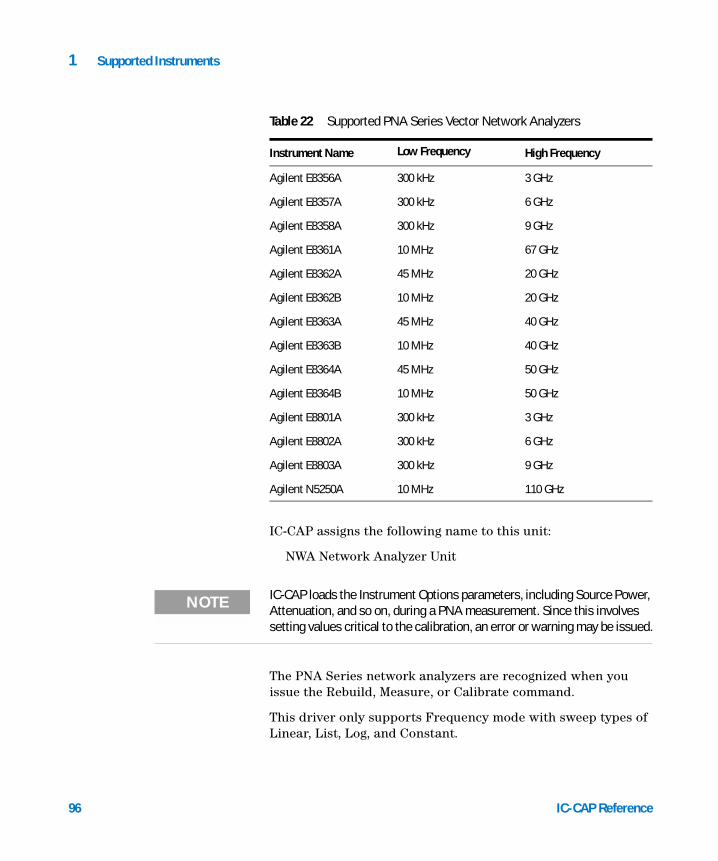
96
1 Supported Instruments
IC-CAP assigns the following name to this unit:
NWA Network Analyzer Unit
Table 22 Supported PNA Series Vector Network Analyzers
Instrument Name Low Frequency High Frequency
Agilent E8356A 300 kHz 3 GHz
Agilent E8357A 300 kHz 6 GHz
Agilent E8358A 300 kHz 9 GHz
Agilent E8361A 10 MHz 67 GHz
Agilent E8362A 45 MHz 20 GHz
Agilent E8362B 10 MHz 20 GHz
Agilent E8363A 45 MHz 40 GHz
Agilent E8363B 10 MHz 40 GHz
Agilent E8364A 45 MHz 50 GHz
Agilent E8364B 10 MHz 50 GHz
Agilent E8801A 300 kHz 3 GHz
Agilent E8802A 300 kHz 6 GHz
Agilent E8803A 300 kHz 9 GHz
Agilent N5250A 10 MHz 110 GHz
NOTE IC-CAP loads the Instrument Options parameters, including Source Power, Attenuation, and so on, during a PNA measurement. Since this involves setting values critical to the calibration, an error or warning may be issued.
The PNA Series network analyzers are recognized when you issue the Rebuild, Measure, or Calibrate command.
This driver only supports Frequency mode with sweep types of Linear, List, Log, and Constant.
IC-CAP Reference

Supported Instruments 1
IC-CAP Reference
• Linear sweep mode allows you to specify the start/stop frequencies, number of points, and step size.
• List sweep mode allows you to sweep up to 202 individual frequencies.
• Log sweep mode allows you to specify start/stop frequencies, number of decades and points per decade. The points are log spaced and you can specify a total of 202 points.
• Constant mode allows you to measure 1 individual frequency.
Table 23 describes the PNA options and their default values, where applicable. For more information on options, refer to the PNA Series Network Analyzer Help file located in the analyzer.
A self-test function is not provided for this instrument.
Calibration
The IC-CAP Calibrate command loads Setup information into the PNA prior to calibrating. When running a measurement afterwards, the calibration set must match IC-CAP’s Setup and it must be valid.
Only hardware calibration is supported. The calibration must be either manually executed or executed using dedicated calibration software and saved in a directory in the PNA. The calibration file must have extension .cst.
NOTE The .cst file type includes the instrument state and a pointer to the internal calset. The .cst file does not save the calibration coefficients (the internal calset). Do not delete the internal calset referenced by the .cst file otherwise the IC-CAP measurement will issue an error.
If you wish to save the calibration coefficients, save the active calset using a .cal file extension. If the internal calset is accidentally deleted, you can reinstate it by loading the .cal file from the front panel. Do this BEFORE running an IC-CAP measurement that uses the .cst file.
To measure calibrated data, set the instrument option Cal Type to H (Hardware) and specify a file name with a .cst extension in the Instrument Option field Cal/State File Name.
97

98
1 Supported Instruments
On the PNA mainframe, the default directory for saving and reading calibration and state file is C:\Program Files\Agilent\Network Analyzer\Documents. You can save the calibration file in a different directory and still recall it from IC-CAP by setting the System Variable PNA_CAL_FILE_PATH to the new directory (use full path such us C:\my_dir\).
When running a measurement recalling a calibration set, the frequency sweep and the instrument options should be consistent with the calibration set. Warnings will be issued in the IC-CAP Status Window when relevant PNA measurement settings (such as IF Bandwidth or Port Power) differ from the calibration settings.
NOTE The PNA has the capability to interpolate between points. Therefore, you can specify a different frequency range and number of points during a measurement as long as the measured frequency range is within the calibrated frequency range. However, be aware that a loss in accuracy occurs due to interpolation.
Table 23 Agilent PNA Options
Option Description
Use User Sweep Yes = use user sweep. No = use instrument’s internal sweep.Default = No
Hold Time Time, in seconds, the instrument waits before each sweep to allow for DC settling.Default = 0
Delay Time Time the instrument waits before setting each frequency in user sweep mode.Default = 0
Sweep Time Time the instrument takes for each sweep. 0 = AutoDefault = 0
Sweep Type[SA] S = Stepped mode. A = Analog (ramp) modeDefault = S
IC-CAP Reference

Supported Instruments 1
IC-CAP Reference
Port Power Coupled Yes = Coupled mode. No = Non-Coupled mode.Default = Yes. When ports are coupled, the Port Src Power value is used for both Port 1 and 2. Port 2 Src Power is ignored. Attenuators are also coupled so that Port Src Atten is used for both ports and Port 2 Src Atten is ignored.
Port Src Power Defines the source Power for Port 1 and 2 when ports are coupled or the source power for Port 1 when ports are uncoupled. The power range depends on the attenuator settings and the PNA model and options.
Port 2 Src Power Defines the source power for Port 2 when ports are uncoupled. This option field is ignored when ports are coupled. The power range depends on the attenuator settings and the PNA model and options.
Port Atten Auto Yes = Auto mode. No = Non-Auto mode.Default = No. When attenuators are in auto-mode, the PNA will set the most efficient values for the attenuators to obtain the requested output power at the port. In auto-mode, the full power range is directly available at the output port. In auto-mode, the instrument options Port Src Atten and Port 2 Src Atten are ignored.
Port Src Atten Possible Values: 0, 10, 20, 30, 40, 50, 60, 70 dBDefault = 0The available range depends on the PNA model. For example, the E8364A attenuator range is 0-60 dB. This option is ignored when attenuators are in auto-mode.
Port 2 Src Atten Possible Values: 0, 10, 20, 30, 40, 50, 60, 70 dBDefault = 0The available range depends on the PNA model. For example, the E8364A attenuator range is 0-60 dB. This option is ignored when attenuators are in auto-mode.
Power Slope Can be any value between –2 and +2 dB/GHzDefault = 0
Dwell Time Sets the dwell time, in seconds, between each sweep point. Only available in Stepped sweep type.Default = 0 (Auto - PNA will minimize dwell time)
Table 23 Agilent PNA Options (continued)
Option Description
99

100
1 Supported Instruments
IF Bandwidth Possible Values: 1, 2, 3, 5, 7, 10, 15, 20, 30, 50, 70, 100, 150, 200, 300, 500, 700, 1k, 1.5k, 2k, 3k, 5k, 7k, 10k, 15k, 20k, 30k, 35k, 40kDefault = 1000 HzNote: If a invalid value is specified, the PNA will not round it to the nearest available value. It will round up to the next higher value.
Avg Factor Number of averages per measurement. [1-1024]Default = 1
Cal Type[HN] H = Hardware calibration. N = No calibrationDefault = N
Cal/State File Name
Name of .cst file (cal file and instrument state) to be used.Default = none
Use PNA Calibration Settings [Yes/No]
This setting can be set to Yes only if a calibration file is available and Calibration Type is set to H (Hardware).Default = NoWhen set to Yes, IC-CAP loads the calibration and runs the measurement without further initializing the instrument (i.e., without downloading the current Instrument Table settings). Although IC-CAP uses the calibration settings for measurements, it still sets the sweep settings (e.g., Start, Stop, Sweep Type, e.t.c.). Therefore, make sure the requested sweep setting is consistent with the calibration settings as IC-CAP attempts to run the measurement without performing any frequency range checking. Also note that when this option is set to Yes, the driver responds as if MEASURE_FAST=Yes (i.e., calibration is loaded only when the measurement is first run or after errors or warnings occur).
Delay for timeouts For long-running measurements (that use a high number of averages, for example) use this option to avoid measurement timeouts.Default = 0
Table 23 Agilent PNA Options (continued)
Option Description
IC-CAP Reference

Supported Instruments 1
IC-CAP Reference
Technical Notes
• You can perform averaging by increasing the number of averages or decreasing the IF filter bandwidth. Both methods result in more samples taken at each frequency point. Decreasing the IF filter bandwidth not only increases the number of samples but also the time at each frequency point resulting in a longer sweep time. Increasing the number of averages, increases the number of sweeps. Although the driver supports both modes, using IF bandwidth for averaging is generally more efficient.
• Coupled ports have the same source power connected to Port 1 and Port 2 for forward and reverse S-parameter measurements. In addition, the attenuator settings are coupled.
• When port attenuators are set to auto mode, the PNA automatically chooses the attenuator value that provides the requested power level at the output port. Accurate S-parameter calibration requires that the attenuator settings do not change during measurements or calibration, therefore auto mode is not recommended.
• If you have significant insertion loss due to cables or bias networks, use power slope. Using the appropriate power slope can compensate for insertion loss as the frequency increases. However, if the network’s return loss is too high, increasing the power slope will not compensate because the power is reflected back.
Init Command Command field to set the instrument to a mode not supported by the option table. Command is sent at the end of instrument initialization for each measurement. Normal C escape characters such as \n (new line) are available.Default = none
Table 23 Agilent PNA Options (continued)
Option Description
101

102
1 Supported Instruments
• Step sweep mode is more accurate than analog (ramp) mode, but analog mode is typically faster than step sweep mode. In step sweep mode, RF phase locking is performed at each frequency, which ensures that the frequency value is very accurate. This results in a longer transition time from 1 frequency point to the next and a longer total sweep time. In analog mode, the RF frequency is swept across the frequency range and its frequency accuracy depends on the linearity of the VCO (Voltage Controlled Oscillator).
• Sweep time is the total time to sweep from Start to Stop frequency. Several factors contribute to sweep time. For example at each point in step mode, sweep time is the summation of transient time due to phase locking, settling time, dwell time, and measurement time, which depends on the IF Bandwidth filter. Although you can specify a sweep time, you should use auto mode (Sweep Time field = 0). This allows the PNA to determine the fastest sweep time based on the other settings. To view the actual sweep time, select Sweep/Sweep Time on the PNA application’s main window. For additional details on sweep time, see the PNA’s online help.
• Dwell time is the time spent at each frequency point before sampling starts. For most applications, you should set dwell time to auto mode. In auto mode, the PNA increases the dwell time as the sweep time increases to comply the total sweep time. If long delays are present in the circuit and additional settling time is needed, set the dwell time to an appropriate value.
Dwell time is not active in analog mode—only in step mode. If the sweep time in analog mode is increased significantly (because of a setting), the PNA can internally switch to step mode and set an optimum value for the dwell time.
HP 3577 Network Analyzer
The HP 3577 has a frequency range of 5 Hz to 200 MHz (100 kHz to 200 MHz with HP 35677A/B S-Parameter Test Set). The RF source is an integral part of this instrument; DC bias levels must be supplied from external sources.
IC-CAP Reference

Supported Instruments 1
IC-CAP Reference
IC-CAP assigns the following name to this unit:
NWA Network Analyzer Unit
Because this instrument does not offer full 2-port calibration, IC-CAP provides a popular 12-term correction for this instrument that is widely used for 2-port measurements. Manual operation is required to measure standards interactively. Separate calibration data can be obtained for each Setup; the data is saved and retrieved when Setups are written to or read from files.
Though IC-CAP supports the HP 3577A and B models, the Discrete Sweep capability of HP 3577B is not available with IC-CAP. Therefore, the log and list frequency sweeps must be performed as a User Sweep.
For most 2-port AC measurements, the network analyzer units must be biased with a current or voltage source to supply DC power to the DUT. A DC analyzer can be used for this. Therefore, a typical S-parameter measurement Setup specification would use the unit name of the network analyzer unit (NWA) in the Unit field of the Output and the unit names of the DC analyzer units in the Unit fields of the biasing Inputs.
NOTE The HP 35677A/B S-Parameter Test Set has a maximum DC bias range of ±30V and ±20mA with some degradation of RF specifications; ±200mA damage level.
The measurement methods, listed in the following table, are selected by setting the Use User Sweep and Use Fast CW flags in the HP 3577 Instrument Options folder.
Table 24 HP 3577 Measurement Modes
Mode Description
Slow CW Sweep Mode
Use User Sweep = Yes. Use Fast CW = NoThe instrument sets each frequency then measures all 4 S-Parameters. Although somewhat slow, this method has the advantage of gathering all of the parameters for a frequency at approximately the same time.
103

104
1 Supported Instruments
The following table describes the HP 3577 options and their default values, where applicable. For more information on options, refer to the HP 3577 Operating and Programming Manual.
Fast CW Sweep Mode
Use User Sweep = Yes. Use Fast CW = YesThis mode is faster than Slow CW Sweep because it performs just 2 user sweeps. The instrument first measures the forward parameters (S11 and S21), then changes the test set direction and measures the reverse parameters (S12 and S22).
Single Freq CW Mode
Use User Sweep = Yes. Use Fast CW = NoThe instrument performs a spot frequency measurement. Except for the number of frequencies, this mode is the same as the Slow CW Sweep Mode.
Internal Sweep Mode
Use User Sweep = NoFastest available sweep type. Sweep must be linear. Values for start, stop, and number of points are stored in the instrument. The number of points in the linear sweep must match 1 of the HP 3577’s allowed number of points choices. When IC-CAP is unable to fit an internal sweep, it attempts to use the Fast CW Mode.
Table 25 HP 3577 Options
Option Description
Use User Sweep Yes = use user sweep. No = use instrument’s internal sweep. Default = No
Hold Time Time, in seconds, the instrument waits before each sweep to allow for DC settling. Default = 0
Delay Time Time the instrument waits before setting each frequency in user sweep mode. Default = 100 msec
Input A Attn Sets Input A attenuation. Choices are 0 or 20 dB. Default = 20 dB
Table 24 HP 3577 Measurement Modes (continued)
Mode Description
IC-CAP Reference

Supported Instruments 1
IC-CAP Reference
The system variables used by the 12-term software calibration are listed in the following table. They primarily affect S11 and S22 corrections at high frequencies. Load and Short standards are assumed ideal in the calibration frequency range. These variables can be defined at Setup or higher levels.Input B Attn Sets Input B attenuation. Choices are 0 or 20 dB. Default = 20 dB
Input R Attn Sets Input R attenuation: 0 or 20 dB. Default = 20 dB
Source Power Source signal level. Range is −45 to 15 dBm. Default = −10 dBm
Sweep Time [.05 - 16]
Instrument internal sweep time, in seconds.Default = 100 msec.
IF Bandwidth Instrument receiver resolution, in Hz. Default = 1000 Hz
Use Fast CW Enables Fast CW mode. Default = Yes
Avg Factor[1-256]
Number of averages per measurement.Default = 1
Cal Type[SN] S = Software calibration. N = No calibration. Default = S
Soft Cal Sequence Software calibration requires measurement of (L)oad, (O)pen, (S)hort, (T)hru, and optionally (I)solation in a certain order. This string defines the sequence of these standard measurements by these letters (L, O, S, T, I). Default = LOST
Delay for Timeouts
For long-running measurements (that use a high number of averages, for example) use this option to avoid measurement timeouts. Default=0
Init Command Command field to set the instrument to a mode not supported by the option table. This command is sent at the end of instrument initialization for each measurement. Normal C escape characters such as \n (new line) are available. Default = none
Table 25 HP 3577 Options (continued)
Option Description
105

106
1 Supported Instruments
Note: CAL_OPEN_C is replaced by CAL_OPEN_C0; CAL_Z0 is replaced by TWOPORT_Z0. Use the new variables when possible; the old variables are effective for the software calibration when the new variables are undefined.
Table 26 System variables
Variable Description
CAL_OPEN_C0CAL_OPEN_C1CAL_OPEN_C2
Define a capacitance of an Open standard in Farads. This value applied to port 1 and port 2. A second-order polynomial is assumed for its frequency response. Copen = C0 + C1 • F + C2 • F2. Default = 0 (for C0, C1, and C2)
TWOPORT_Z0 Defines impedance of port 1 and port 2, in Ohms. This and the open capacitance value are used to calculate open gamma correction data. Also used by TwoPort function. Default = 50 Ohms
HP/Agilent 8510 Network Analyzer
The HP/Agilent 8510 is identical to the HP 8753 except:
• The 8510A has a frequency range of 45 MHz to 26.5 GHz.
• The 8510B options can source frequencies up to 100 GHz.
• The RF source is a separate external instrument.
• The 8510A does not support frequency list mode—it cannot run internal log and list sweeps.
IC-CAP assumes an A model if the instrument is manually added to the Instrument List (in the Hardware Setup window) by selecting it and clicking the Add button. For IC-CAP to recognize a newer model, use the Rebuild command or perform a dummy measurement: use a linear sweep with the Use Linear List option set to No. Note that the 8510C is treated as the B model.
IC-CAP assigns the following name to this unit:
NWA Network Analyzer Unit
IC-CAP Reference

Supported Instruments 1
NOTE IC-CAP loads the Instrument Options parameters, including Source Power, Attenuation, and so on, during an 8510 measurement. Because this involves setting values critical to the calibration, the following warning may be issued: Calibration may be invalid.
If the IC-CAP Calibrate command is used to load Setup information to the 8510 prior to calibrating, the calibration set must match IC-CAP’s Setup and be valid.
IC-CAP Reference
For information on the processes listed below, refer to the section, “HP 3577 Network Analyzer” on page 102.
• Use of DC bias sources
• Available measurement modes
• System variables used in software calibration
NOTE Use the 12-term software calibration carefully at very high frequencies where accuracy of the Load termination generally degrades.
The following table describes the 8510 options and their default values, where applicable. For more information on options, refer to the HP 8510 Operating and Programming Manual.
Table 27 HP/Agilent 8510 Options
Option Description
Use User Sweep Yes = use user sweep. No = use instrument’s internal sweep. Default = Yes
Hold Time Time, in seconds, the instrument waits before each sweep to allow for DC settling. Default = 0
Delay Time Time the instrument waits before setting each frequency in user sweep mode. Default = 100 msec
Port 1 Attn Sets Port 1 attenuation. This option is ignored by the 8510XF. Range is 0 to 90 dB. Default = 20 dB
107
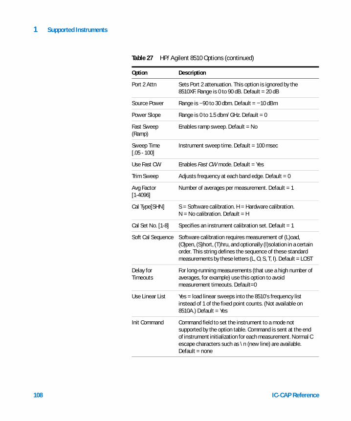
108
1 Supported Instruments
Port 2 Attn Sets Port 2 attenuation. This option is ignored by the 8510XF. Range is 0 to 90 dB. Default = 20 dB
Source Power Range is −90 to 30 dbm. Default = −10 dBm
Power Slope Range is 0 to 1.5 dbm/GHz. Default = 0
Fast Sweep (Ramp)
Enables ramp sweep. Default = No
Sweep Time[.05 - 100]
Instrument sweep time. Default = 100 msec
Use Fast CW Enables Fast CW mode. Default = Yes
Trim Sweep Adjusts frequency at each band edge. Default = 0
Avg Factor [1-4096]
Number of averages per measurement. Default = 1
Cal Type[SHN] S = Software calibration. H = Hardware calibration.N = No calibration. Default = H
Cal Set No. [1-8] Specifies an instrument calibration set. Default = 1
Soft Cal Sequence Software calibration requires measurement of (L)oad, (O)pen, (S)hort, (T)hru, and optionally (I)solation in a certain order. This string defines the sequence of these standard measurements by these letters (L, O, S, T, I). Default = LOST
Delay for Timeouts
For long-running measurements (that use a high number of averages, for example) use this option to avoid measurement timeouts. Default=0
Use Linear List Yes = load linear sweeps into the 8510’s frequency list instead of 1 of the fixed point counts. (Not available on 8510A.) Default = Yes
Init Command Command field to set the instrument to a mode not supported by the option table. Command is sent at the end of instrument initialization for each measurement. Normal C escape characters such as \n (new line) are available. Default = none
Table 27 HP/Agilent 8510 Options (continued)
Option Description
IC-CAP Reference

Supported Instruments 1
IC-CAP Reference
When performing 2 sequential CW measurements that use different CW cal subsets, the 8510 may report the error RF UNLOCKED. A system variable is available in IC-CAP, in the Measurement Options group, to ignore this error:
IGNORE_8510_RF_UNLOCK
When defined as Yes, IC-CAP ignores a temporary and benign RF UNLOCKED error from the 8510.
Making Measurements with Uncoupled Ports
To calibrate using the 8510XF driver:
1 Set input sweeps and instrument options. To set port 1 power, set Source Power. To set port 1 power slope, set Power Slope. Set averaging. Ignore the Port 1 and 2 Attenuators fields as the 8510XF does not have attenuators.
2 In the Init Command field, type the following command string to set port 2 power and slope:PPCOUPLEOFF;POWP2 <power>SLPP2ON <slope>
Example:PPCOUPLEOFF;POWP2 -20;SLPP2ON 0.05;
sets P2=-20 dB and Power slope 2 to 0.05 dB/GHz
3 Click Calibrate. This downloads the sweep settings, the instrument option settings, and sets the 8510XF with uncoupled ports.
4 Perform RF Calibration and save the results in one of the Calsets.
When making a measurement using the 8510XF driver, the driver recalls the calibration data and the setting used during calibration. If you want to use the same power level and slope, you do not need to make any changes. If you want to change the port 2 power setting, use the Init Command field as in step 2 (you do not need PPCOUPLEOFF since the ports are already off when calibration is recalled). Be aware that the 8510XF will issue a warning if you set a different port power for the measurements.
109

1 Supported Instruments
HP/Agilent 8702 Network Analyzer
110
The HP/Agilent 8702 network analyzer has a frequency range of 300 kHz to 3 GHz (IC-CAP does not support the lightwave analyzer features). Use Option 006 and turn on the frequency doubler from the front panel if 6 GHz is desired. The RF source is an integral part of this instrument. For other features, refer to the section, “HP/Agilent 8753 Network Analyzer” on page 114 because the HP/Agilent 8702 is almost identical to the HP/Agilent 8753 in the E/E mode. IC-CAP supports both HP/Agilent 85046A and HP/Agilent 85047A S-Parameter Test Sets for the HP/Agilent 8702.
IC-CAP assigns the following name to this unit:
NWA Network Analyzer Unit
For most 2-port AC measurements, the network analyzer units must be biased with a current or voltage source to supply DC power to the DUT. A DC analyzer can be used to supply this current or voltage source. Therefore, a typical S-parameter measurement Setup specification would use the unit name of the network analyzer unit (NWA) in the Unit field of the Output and the unit names of the DC analyzer units in the Unit fields of the biasing Inputs.
For information on the topics listed below, refer to the section, “HP/Agilent 8753 Network Analyzer” on page 114.
• Measurement modes
• Options
NOTE The 8702 occupies 2 GPIB addresses, the instrument itself and the display. The display address is derived from the instrument address by complementing the least significant bit. Hence, if the instrument is at an even address, the display occupies the next higher address; if the instrument is at an odd address, the display occupies the next lower address.
IC-CAP Reference

Supported Instruments 1
HP/Agilent 8719 Network Analyzer
IC-CAP Reference
The HP/Agilent 8719 is identical to the HP/Agilent 8720 except the 8719 has a frequency range of 50 MHz to 13.5 GHz. For information, refer to the next section, “HP/Agilent 8720 Network Analyzer.”
HP/Agilent 8720 Network Analyzer
The HP/Agilent 8720 network analyzer has a frequency range of 50 MHz to 20 GHz. The RF source and S-parameter test set are an integral part of this instrument. IC-CAP supports the HP/Agilent 8720 A, B, C, and D models. (The 8720 D is the only model that supports uncoupled port power.)
IC-CAP assigns the following name to this unit:
NWA Network Analyzer Unit
NOTE The 8720 occupies 2 GPIB addresses, the instrument itself and the display. The display address is derived from the instrument address by complementing the least significant bit. Hence, if the instrument is at an even address, the display occupies the next higher address; if the instrument is at an odd address, the display occupies the next lower address.
For most 2-port AC measurements, the network analyzer units must be biased with a current or voltage source to supply DC power to the DUT. A DC analyzer can be used to supply this current or voltage source. Therefore, a typical S-parameter measurement Setup specification would use the unit name of the network analyzer unit (NWA) in the Unit field of the Output and the unit names of the DC analyzer units in the Unit fields of the biasing Inputs.
Measurement modes for the 8720 are the same as for the 8753; refer to Table 29 for this information.
For system variables used in the software calibration, refer to Table 26 in the HP 3577 section.
111

112
1 Supported Instruments
The following table describes the 8720 options and their default values, where applicable.
Table 28 HP/Agilent 8720 Options
Option Description
Use User Sweep Yes = use user sweep. No = use instrument’s internal sweepDefault = No
Hold Time Time, in seconds, that the instrument waits before each sweep to allow for DC settling. Default = 0
Delay Time Time the instrument waits before setting each frequency. Default = 100 msec
Port 1 Source Power
Range is −65 to 10 dBm. Default = −10.00 dBm
Port 1 Power Range
Specifies which instrument power range to use. Range is 1 to 12 for models A, B, and C; range is 0 to 11 for model D. (The Hardware calibration is turned off by the instrument when calibrated Power Range and requested Power Range don’t match.) Default = 1
Port 1 Auto Power Range†
Enables auto power ranging on port 1. Default = Yes
Coupled Port Power†
Enables/disables coupled test port power. When disabled, Port 2 options are ignored. Default = Yes
Port 2 Source Power†
Range is −65 to 10 dBm. Default = −10.00
Port 2 Power Range†
Specifies which instrument power range to use. Range is 1 to 12 for models A, B, and C; range is 0 to 11 for model D. (The Hardware calibration is turned off by the instrument when calibrated Power Range and requested Power Range don’t match.) Default = 1
Port 2 Auto Power Range†
Enables auto power ranging on port 2. Default = Yes
Sweep Time Instrument sweep time. A zero sweep time turns on the Auto Sweep Time, which ensures the minimum sweep time. Default = 100 msec
IC-CAP Reference

Supported Instruments 1
IC-CAP Reference
† These options apply only when using built-in test set (Model D).IF Bandwidth (Avg)
Instrument’s receiver IF bandwidth. Default = 1000 Hz
Use Fast CW Enables Fast CW mode. Default = Yes
Avg Factor [1-999] Number of averages per measurement. Default = 1
Cal Type[SHN] S = Software calibration. H = Hardware calibration.N = No calibration. Default = H
Cal Set No. Models A, B, and C: 1 through 5 specifies which instrument calibration sets to use; 6 specifies the active instrument state. Model D: 1 through 32 specifies which instrument calibration sets to use; 33 specifies the active instrument state. Default = 1
Soft Cal Sequence Software calibration requires measurement of (L)oad, (O)pen, (S)hort, (T)hru, and optionally (I)solation in a certain order. This string defines the sequence of these standard measurements by these letters (L, O, S, T, I). Default = LOST
Delay for Timeouts
For long-running measurements (that use a high number of averages, for example) use this option to avoid measurement timeouts. Default=0
Use Linear List Yes = load linear sweeps into the HP/Agilent 8720’s frequency list instead of one of the fixed point counts. This mode should be faster than using the instruments linear frequency sweep. Default = Yes
Init Command Command field to set the instrument to a mode not supported by the option table. This command is sent at the end of instrument initialization for each measurement. Normal C escape characters such as \n (new line) are available. Default = none
Table 28 HP/Agilent 8720 Options (continued)
Option Description
HP/Agilent 8722 Network Analyzer
The HP/Agilent 8722 is identical to the HP/Agilent 8720 except for its frequency range—the HP/Agilent 8722 has a frequency range of 50 MHz to 40 GHz.
113

1 Supported Instruments
HP/Agilent 8753 Network Analyzer
114
The HP/Agilent 8753 network analyzer has a frequency range of 300 kHz to 3 GHz (6 GHz with Option 006). The instrument contains an RF source for frequency sweeps, but DC bias must be supplied from external sources to acquire biased RF data.
IC-CAP assigns the following name to this unit:
NWA Network Analyzer Unit
IC-CAP supports the HP/Agilent 8753 A, B, C, D, E, and D opt 011 models (D models must be firmware revision 6.14 or higher). The standard D and E models have a built-in test set; the A, B, C, and D opt 011 models are used in conjunction with an external test set. IC-CAP supports both the HP/Agilent 85046A and HP/Agilent 85047A S-Parameter Test Sets.
NOTE IC-CAP cannot differentiate between model D and D opt 011. When using the 8753D with an external test set, alias it as an 8753C in the instraliases file in the $ICCAP_ROOT/iccap/lib directory.
NOTE The 8753 occupies 2 GPIB addresses, the instrument itself and the display. The display address is derived from the instrument address by complementing the least significant bit. Hence, if the instrument is at an even address, the display occupies the next higher address; if the instrument is at an odd address, the display occupies the next lower address.
The model is recognized when you issue the Rebuild, Measure, or Calibrate command. If you manually add the instrument to the active instrument list (by clicking the Add button), IC-CAP assumes the instrument is an A model until one of the previously described commands is issued.
IC-CAP Reference

Supported Instruments 1
NOTE Some early models of the 8753C (ROM 4.00 and 4.01) have GPIB problems that prevent IC-CAP from finding this instrument during Rebuild. Add the instrument manually after PRESET when IC-CAP ignores this instrument. The model is recognized when Measure or Calibrate is performed.
IC-CAP Reference
A self-test function is not provided for this instrument.
For most 2-port AC measurements, the network analyzer units must be biased with a current or voltage source to supply DC power to the DUT. A DC analyzer can be used to supply this current or voltage source. Therefore, a typical S-parameter measurement Setup specification would use the unit name of the network analyzer unit (NWA) in the Unit field of the Output and the unit names of the DC analyzer units in the Unit fields of the biasing Inputs.
Hardware calibration is only supported when using Internal Sweep mode or Single Freq CW mode. For measurement modes that do not support internal instrument calibration, software calibration is provided. When software calibration is set in the instrument options, use the Calibrate command to initiate the calibration. IC-CAP will load the frequency values and options into the instrument and then direct you to connect the various calibration standards required to perform the calibration.
The Calibrate command can also be used to download the desired instrument state when requesting a hardware calibration You must then calibrate the instrument manually (refer to the instrument manual) and store the results in one of the instrument’s state registers. With this method there is no need to manually input the instrument state to match the IC-CAP settings.
The measurement modes listed in Table 29 are selected by setting a combination of the following fields (details follow) in the 8753 Instrument Options folder:
• Use User Sweep
• Use Fast CW
• Use Linear List
• Cal Type field
115

116
1 Supported Instruments
IC-CAP contains routines that compare its sweep values with those stored in the 8753. In case of discrepancies, IC-CAP prompts you to specify whether the sweeps should be modified to match the instrument. This may not be practical when variables are included in the sweep specifications.
Error checking ensures a valid measurement mode. When discrepancies are found, the following changes are made:
• For CON frequency, Use User Sweep is set to Yes and Use Fast CW is set to No.
• For internally calibrated sweeps, Use User Sweep is set to No.
• When frequency is not the main sweep, Use Fast CW is set to No, Cal Type is set to N, and Use User Sweep is set to Yes.
Refer to “HP 3577 Network Analyzer” on page 102 for system variables used in the software calibration.
Table 30 describes the 8753 options and their default values, where applicable. Differences in options when using the 8753 with an external test set versus a built-in test set are noted.
For optimum performance of the HP/Agilent 85047 test set, 6 GHz mode requires Source Power to be +20dBm. The Instrument Options folder should show 20 as the Source Power level when the Freq Range is 6 GHz. Setting Source Power to less than 20 can cause No IF Found errors in the 8753. Further information on the power requirements for 6 GHz operation can be found in the instrument’s operation manual.
When the test set switches between 3 and 6 GHz operation, the 8753 automatically changes Source Power level.
• 3 to 6 GHz Switching: 20 dBm.
• 6 to 3 GHz Switching: 0 dBm.
When Hardware calibration is used, a specified calibration set recalls the original calibration power level. When Software or no calibration is used, the Source Power will be forced to one of the default levels if the test set has to switch modes. When a Source Power level other than the above forced values is required, perform one of the following:
• Make a dummy measurement first to switch the test set to the desired frequency mode
IC-CAP Reference

Supported Instruments 1
IC-CAP Reference
• Manually switch the test set to the desired frequency mode
• Use the Calibrate command to download the desired instrument state
NOTE The 8753 may not reflect the power level specified in the Instrument Options folder if the analyzer is in HOLD mode. When the 8753 is in HOLD mode and receives a remote command to switch the frequency mode of the test set, it postpones switching modes until an actual measurement sweep is triggered. When the Measure or Calibrate command is issued, IC-CAP initializes the state before triggering a measurement. Thus IC-CAP will download the power level specified in the Instrument Options folder and the analyzer will force it to its default value when the measurement is triggered.
For descriptions of the variables used in software calibration, refer to Table 26 in the HP 3577 Network Analyzer section.
Table 29 Supported Measurement Modes
Mode Description Use User Sweep
Use Fast CW
Use Linear List
Cal Type
Slow CW Sweep
IC-CAP performs a spot measurement of 2-port data by setting the instrument to each frequency point individually and measuring all 4 S-parameters. Although slow, this method has the advantage of gathering all of the parameters for a frequency at approximately the same time. Only uncalibrated data can be obtained from this type of measurement since each frequency point is measured in CW mode. Typically used when frequency is not the primary sweep (Sweep Order ≠ 1).
Yes No Ignored S, N
117

118
1 Supported Instruments
Notes:† For linear sweeps, the number of points requested must fit one of the 8753's predefined number of points. If the desired number of points is not one of the legal set values, IC-CAP checks to see if it still can make a valid measurement by increasing the number of points on the instrument such that data at the desired frequencies can be acquired. For example, a 300 to 500 kHz sweep in 6 steps internally requires IC-CAP to set the instrument to 11 points because 11 is a legal value. When IC- CAP is unable to fit an internal sweep, it attempts to use the Fast CW mode. If CW mode is not desired, set Use Linear List = Yes.
For log and list sweeps, set Use Linear List = Yes. This uses the instrument's frequency list capability. Because the 8753 is limited to thirty sub-sweeps, it can
Fast CW Sweep
Similar to Slow CW Sweep, this mode is faster because it first measures the forward parameters (S11 and S21) with a single sweep, then the reverse parameters (S12 and S22). This is accomplished by using the dual channel feature of the instrument. As with Slow CW Sweep, instrument calibration is not possible and only uncalibrated data can be obtained.
Yes Yes Ignored S, N
Single Freq CW
This is the only user sweep mode capable of acquiring 2-port data using hardware calibration. A CW mode calibration can be performed and saved in one of the state registers to be recalled when a measurement is executed.
Yes No Ignored H,S,N
Internal Sweep
Fastest available sweep type. Sweeps can be linear, log, or list.
†
Since this is an internal sweep, hardware calibration is possible. IC-CAP expects that the calibration over the appropriate frequencies has been completed before the measurement is performed.
No No Yes or No
H,S,N
Table 29 Supported Measurement Modes (continued)
Mode Description Use User Sweep
Use Fast CW
Use Linear List
Cal Type
IC-CAP Reference

Supported Instruments 1
IC-CAP Reference
store no more than sixty frequencies.Instrument options must match those for which the 8753 was calibrated.
Table 30 Options for the HP/Agilent 8753
Option Description
Use User Sweep Yes = use user sweep. No = use instrument's internal sweep Default = No
Hold Time Time, in seconds, the instrument waits before each sweep to allow for DC settling. Default = 0
Delay Time Time the instrument waits before setting each frequency. Default = 100 msec
Port 1 Atten† Sets Port 1 attenuation. Range is 0 to 70 dB. Default = 20 dB
Port 2 Atten† Sets Port 2 attenuation. Range is 0 to 70 dB. Default = 20 dB
Source Power† Range is −10 to 25 dbm. Default = −10
Power Slope Models A, B, C, and D opt 11: Range is 0 to 2 dbm/GHz. Default = 0Models D and E: Range is −2 to +2dBm/GHz. Default = 0 dBm/GHz
Port 1 Source Power††
Sets Port 1 source power level. Range is −85 to +10 dBm. Default = −10 dBm
Port 1 Power Range[0-7]††
Sets Port 1 source power range. The valid range is 0 to 7. Default = 0
Port 1 Auto Power Range††
Enables auto power ranging on port 1. Default = No
Coupled Port Power††
Enables/disables coupled test port power. When disabled, Port 2 options are ignored. Default = Yes
Port 2 Source Power††
Sets Port 2 source power level. Range is −85 to +10 dBm. Default = −10 dBm
Port 2 Power Range[0-7]††
Sets Port 2 source power range. The valid range is 0 to 7. Default = 0
119

120
1 Supported Instruments
Port 2 Auto Power Range††
Enables auto power ranging on port 2. Default = No
Sweep Time Instrument sweep time. Zero sweep time turns on the Auto Sweep Time, which ensures the minimum sweep time. Default = 100 msec
IF Bandwidth (Avg)
Instrument receiver IF bandwidth setting in the Averaging menu. Default = 1000 Hz
Use Fast CW Enables Fast CW mode. Default = Yes
Avg Factor [1-999]
Number of averages per measurement. Default = 1
Cal Type [SHN] S = Software calibration. H = Hardware calibration. N = No calibration. Default = H
Cal Set No. Models A, B, C, and D opt 11: 1 through 5 specifies which instrument calibration sets to use; 6 specifies the active instrument state. Models D and E: 1 through 32 specifies which instrument calibration sets to use; 33 specifies the active instrument state. Default = 1
Soft Cal Sequence Software calibration requires measurement of (L)oad, (O)pen, (S)hort, (T)hru, and optionally (I)solation in a certain order. This string defines the sequence of these standard measurements by these letters (L, O, S, T, I). Default = LOST
Delay for Timeouts
For long-running measurements (that use a high number of averages, for example) use this option to avoid measurement timeouts. Default=0
Use Linear List Yes = load linear sweeps into the 8753 frequency list instead of one of the fixed point counts. This mode should be faster than using the instrument’s linear frequency sweep. Default = Yes
Freq Range [36N]† This option sets Frequency Range to 3 GHz, 6 GHz, or No change. Default = N
Table 30 Options for the HP/Agilent 8753 (continued)
Option Description
IC-CAP Reference

Supported Instruments 1
IC-CAP Reference
Notes:† These options apply only when using external test set (Models A, B, C, and D opt 11).†† These options apply only when using built-in test set (Models D and E).
Init Command This command field sets the instrument to a mode that is not supported by the option table. This command is sent at the end of instrument initialization for each measurement. Normal C escape characters such as \n (new line) are available. Default = none
Table 30 Options for the HP/Agilent 8753 (continued)
Option Description
121

1 Supported Instruments
Wiltron360 Network Analyzer
122
The Wiltron360 network analyzer has a frequency range of 10 MHz to 60 GHz depending on the RF source. If the frequency sweep requested exceeds the limits of the source, IC-CAP issues an error message, Parameter Out of Range. Check Inputs. The RF source is an integral component of the system for frequency sweeps, but DC bias must be supplied from external sources to acquire biased RF data.
The Wiltron360 can be added to the active instrument list by issuing the Rebuild command from the Hardware Setup window. If the Wiltron360 is manually added to the active instrument list using the Add button, IC-CAP verifies that the instrument is available on the bus when either the Measure or Calibrate command is first issued.
IC-CAP assigns the following name to this unit:
NWA Network Analyzer Unit
IC-CAP supports only hardware calibration for this instrument. After a broadband calibration, the 360 can perform a spot measurement of swept calibrated data—software calibration is not required. This capability also allows a CON frequency input defined in an IC-CAP setup to be used with a broadband calibration. For either measurement method, the requested frequency points must be a subset of the frequency sweep currently set up on the instrument. If the requested frequency point is not part of the instrument sweep, IC-CAP will issue an error message.
The measurement modes listed in Table 31 are selected by setting the following fields in the Wiltron360 Instrument Options folder:
• Use User Sweep
• CW Mode Setup
• Cal Type
IC-CAP Reference

Supported Instruments 1
IC-CAP Reference
IC-CAP supports recalling calibration sets from the Wiltron360 internal disk drive. The Cal File Name option is provided to recall the desired calibration state from disk. If no calibration file name is supplied, the current active instrument state is used.
IC-CAP loads the Instrument Options parameters during a measurement. Because this involves setting stimulus values sensitive to the calibration, instrument options must match those for which the Wiltron360 was calibrated; otherwise, the Wiltron360 will issue a Calibration may be invalid message if any of the downloaded stimulus values are different from the current calibration. If this message is displayed, check the Instrument Options folder to verify which value is different and modify as appropriate. Use the Calibrate command from the Setup menu to download the options information to the Wiltron360 prior to calibrating. This ensures that the calibration will match IC-CAP’s Setup and be valid.
Table 31 Measurement Modes
Mode Description Use User Sweep
CW Mode Setup
Cal Type
CW Sweep
Used when frequency is not the primary sweep (Sweep Order = 1). IC-CAP performs a spot measurement of 2-port data by setting the instrument to each frequency point individually and measuring all S-parameters. A broadband hardware calibration can be performed. The calibration does not have to match the IC-CAP sweep exactly; however, the desired swept frequency points must be a subset of the calibrated frequencies.
Yes No H or N
Single Freq CW
Used when a CW mode hardware calibration is performed.
Yes Yes H
123

124
1 Supported Instruments
The following table describes the Wiltron360 options and their default values, where applicable.
Internal Sweep
Linear, log, or list sweeps. Hardware calibration over requested frequencies is completed before an IC-CAP measurement is performed. Unlike CW Sweep, the calibration frequencies must match the setup.
No No H or N
Table 32 Wiltron360 options
Option Description
Use User Sweep Yes = Use user sweep No = use instrument's internal sweep. Default = No
Hold Time Time, in seconds, the instrument waits before each sweep to allow for DC settling. Default = 0
Delay Time Time the instrument waits before setting each frequency in user sweep mode. Default = 50 msec
Port 1 Src Atten
Sets Port 1 source attenuation. Range is 0 to 70 dB, in 10 dB increments. Default = 0 dB
Port 2 Src Atten
Sets Port 2 source attenuation. Range is 0 to 70 dB, in 10 dB increments. Default = 0 dB
Port 2 Test Atten
Sets test port attenuation (port 2). Range is 0 to 40 dB, in 10 dB increments. Default = 0 dB
Source Power Range is dependent on test set used. Default = 0 dBm
IF Bandwidth [NRM]
Sets instrument's receiver IF Bandwidth. N = NormalR = Reduced M = Minimum. Default = N
Avg Factor [1-4095]
Sets number of averages per measurement Default = 1
Use CW Mode Setup
Indicates to IC-CAP that NWA has been set up in single point (CW) measurement mode. Default = No
Table 31 Measurement Modes
Mode Description Use User Sweep
CW Mode Setup
Cal Type
IC-CAP Reference

Supported Instruments 1
IC-CAP Reference
Cal Type[HN] H = Hardware calibration N = No calibration Default = H
Cal File Name Specifies instrument calibration file to recall. If hardware calibration is requested and this option is empty, IC-CAP will use the current active instrument state. Default = Null
Soft Cal Sequence Software calibration requires measurement of (L)oad, (O)pen, (S)hort, (T)hru, and optionally (I)solation in a certain order. This string defines the sequence of these standard measurements by these letters (L, O, S, T, I). Default = LOST
Delay for Timeouts
For long-running measurements (that use a high number of averages, for example) use this option to avoid measurement timeouts. Default=0
Init Command Command field to set to a mode not supported by the option table. This command is sent at the end of instrument initialization for each measurement. Normal C escape characters such as \n (new line) are available. Default = none
System Variables None. Software calibration is not provided for the Wiltron360.
Table 32 Wiltron360 options (continued)
Option Description
125

1 Supported Instruments
Oscilloscopes
126
The oscilloscopes supported by IC-CAP are:
• HP 54120T Series Digitizing Oscilloscopes
• HP 54510 Digitizing Oscilloscope
• Agilent Infiniium Oscilloscope
• HP 54750 Series Digitizing Oscilloscopes
HP 54120T Series Digitizing Oscilloscopes
The HP 54120 Series of digitizing oscilloscopes measure time-domain responses, including TDR (time-domain reflectometry).
• HP 54121T measures signals from DC through 20 GHz.
• HP 54122T (does not have a step generator and cannot perform TDR measurements) provides programmable input attenuation. Bandwidth is reduced to 12.4 GHz due to the input attenuators.
• HP 54123T operates up to 34 GHz; it operates up to 20 GHz on channel 1 (the channel on which the step generator is available).
IC-CAP assigns the following names to the units:
CHn Channel Unit n (1, 2, 3, and 4)
A Setup configured for measurements using an HP 54120 Series is in the model file 54120.demo.mdl. See Appendix G, “54120 Demo” for additional information about this demonstration file. These files also include examples using an HP 54120 Series oscilloscope with an HP 8130 pulse generator and provides hints for obtaining good alignment between measured and simulated waveforms when a pulse generator is used.
The following instrument capabilities are supported by IC-CAP:
• Time-domain measurements nested within DC bias settings provided by DC SMUs.
• 4-channel concurrent data acquisition.
IC-CAP Reference

Supported Instruments 1
IC-CAP Reference
• Offset, range, and probe attenuation adjustment for each channel. HP 54122T includes options to set internal attenuation for each channel (refer to Table 33).
• Averaging of between 1 and 2048 waveform acquisitions on each channel.
• Automatic Pulse Parameter Measurements, such as risetime and peak-to-peak voltage. These are requested in Outputs of Mode T. For help on the available choices, click the middle mouse button over the Pulse Param field and see the Status window.
• Square-wave generation (except HP 54122T) on CH1, the left-most connector on the test set. Frequency can be adjusted from 15.3 Hz to 500 kHz. To activate the step generator, the Setup should include an Input with Mode V and Type TDR. In the absence of a type TDR Input, the step generator is not activated.
The instruments do not support some of the fields present in a TDR Input. For example, it is not possible for the instrument to offer other than a 50-ohm source impedance. The one field that is of consequence to oscilloscope measurements is Period. IC-CAP directs the instrument to use the closest value supported.
The other TDR Input fields are ignored during measurement, and the following hardware-imposed values of the instrument’s step function apply:
• Initial value of 0V
• Pulsed value of 200 mV into 50 ohms; 400 mV into an open-circuit
• Delay of approximately 17 nsec
• Risetime of approximately 40 psec
• Pulse width equal to about 50 percent of the specified period
• Source impedance of 50 ohms
• Time-Domain Reflectometry (except HP 54122T). When a type TDR Input is present in the Setup, the reflected signal is available on the unit designated CH1.
127

128
1 Supported Instruments
To make a time-domain measurement, a Setup must have these inputs and outputs:
• An Input with Mode T and Type LIN. Here, the values of Start, Stop, and Number of Points govern the time axis of the measurement. Start and Stop values define the time viewing window, and are relative to the trigger event used by the oscilloscope.
• Optionally, an Input of Mode V and Type TDR or PULSE. The Period field in this Input controls the rate of the oscilloscope’s internal square-wave generator. If Period is set to 0, or if this Input is absent from the Setup, the oscilloscope’s internal square-wave generator is not activated for the measurement. In this case, a trigger signal must be provided on the oscilloscope’s trigger input.
If the Input’s Unit field is set to ground, IC-CAP ignores the Input during the measurement. In this manner, measurements can be performed using a pulse generator controlled by its front panel. If the Input’s Unit field is set to the pulse unit of a supported pulse generator (for example, PULSE1 for an HP 8130 generator), then IC-CAP will control the pulse generator to provide stimulus to the DUT and oscilloscope.
Refer to the HP 8130 Pulse Generator documentation provided with IC-CAP.
• To capture a waveform from any of the instrument’s 4 channels requires an Output of Mode V. The Output Editor permits you to specify from which channel a waveform is desired. Define an Output for each channel of interest.
• To obtain automatically extracted pulse parameters at any of the 4 channels requires an Output of Mode T.
The following pulse parameters can be requested: DUTYCYCLE, FALLTIME, FREQ, OVERSHOOT, PERIOD, PRESHOOT, RISETIME, VPP, VRMS, +WIDTH, and -WIDTH. Consult the instrument’s Front Panel Operation Reference for definitions of these parameters or information on the process by which the instrument computes them.
IC-CAP Reference
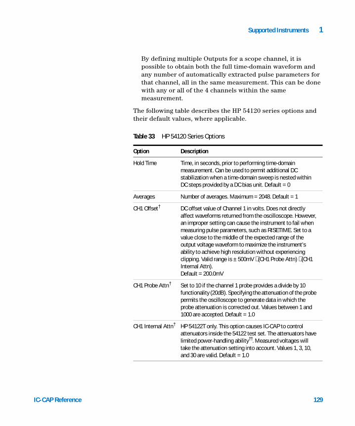
Supported Instruments 1
IC-CAP Reference
By defining multiple Outputs for a scope channel, it is possible to obtain both the full time-domain waveform and any number of automatically extracted pulse parameters for that channel, all in the same measurement. This can be done with any or all of the 4 channels within the same measurement.
The following table describes the HP 54120 series options and their default values, where applicable.
Table 33 HP 54120 Series Options
Option Description
Hold Time Time, in seconds, prior to performing time-domain measurement. Can be used to permit additional DC stabilization when a time-domain sweep is nested within DC steps provided by a DC bias unit. Default = 0
Averages Number of averages. Maximum = 2048. Default = 1
CH1 Offset† DC offset value of Channel 1 in volts. Does not directly affect waveforms returned from the oscilloscope. However, an improper setting can cause the instrument to fail when measuring pulse parameters, such as RISETIME. Set to a value close to the middle of the expected range of the output voltage waveform to maximize the instrument’s ability to achieve high resolution without experiencing clipping. Valid range is ± 500mV ⋅ (CH1 Probe Attn) ⋅ (CH1 Internal Attn). Default = 200.0mV
CH1 Probe Attn† Set to 10 if the channel 1 probe provides a divide by 10 functionality (20dB). Specifying the attenuation of the probe permits the oscilloscope to generate data in which the probe attenuation is corrected out. Values between 1 and 1000 are accepted. Default = 1.0
CH1 Internal Attn† HP 54122T only. This option causes IC-CAP to control attenuators inside the 54122 test set. The attenuators have limited power-handling ability††. Measured voltages will take the attenuation setting into account. Values 1, 3, 10, and 30 are valid. Default = 1.0
129

130
1 Supported Instruments
Notes:† Option table entries are also provided for Offset, Probe Attn, Internal Attn, and Range on channels CH2, CH3, and CH4.††Changing the Probe Attn options for CH1-CH4 and the trigger input does not attenuate the input signals. It only changes the results reported by the instrument. To deliver signals exceeding 2V DC or 16 dBm AC peak, use an external attenuator.
By using the internal attenuators of the HP 54122T (via the Internal Attn options), larger voltages can be accepted. Limitations on attenuator voltage and power handling are described in the Internal Atten documentation in the Channels Menu chapter of the HP 54122T Front Panel Reference.
CH1 Range† Set in excess of the maximum anticipated signal swing for this channel. Does not affect waveforms returned from the oscilloscope. However, an improper setting can cause the instrument to fail when measuring pulse parameters, such as RISETIME. Specify a Range value between
CH1 Range†
(cont’d)8mV ⋅ (CH1 Probe Attn) ⋅ (CH1 Internal Attn) and 640mV ⋅ (CH1 Probe Attn) ⋅ (CH1 Internal Attn). Default = 640.0 mV
Table 33 HP 54120 Series Options (continued)
Option Description
NOTE The external trigger is ignored if a TDR type Input is defined in the Setup. In the presence of a TDR type Input, the scope is triggered by its internal TDR step generator.
The TRG options listed in the following table apply when driving the trigger input of the oscilloscope with an external signal. This is typically done with the trigger output from a signal generator.
Table 34 Trigger Options for the HP 54120T Series
Option Description
TRG Probe Attn Set to 10 if the trigger probe is fitted with a 10X (20dB) divider. Values between 1 and 1000 are accepted. Default = 1.0
IC-CAP Reference

Supported Instruments 1
IC-CAP Reference
TRG Slope Specify triggering on a rising (+) or falling (−) edge. Default = +
TRG Level Voltage threshold at which triggering occurs. Valid range is ±1V ⋅ (TRG Probe Attn). Default = 100.0mV
Normalize TDR If Yes, TDR waveform data from CH1 is subject to the HP 54120 series reflection normalization process. This can substantially improve waveform integrity when cabling and test fixtures have impedance mismatches. Prior to using this option perform calibration of the network reflection path via the front panel Network page. Default = No (This option is not supported by the HP 54122.)
Delay for Timeouts
For long-running measurements (that use a high number of averages, for example) use this option to avoid measurement timeouts. Default=0
Init Command Command field to set the instrument to a mode not supported by the option table. This command is sent at the end of instrument initialization for each measurement. Normal C escape characters such as \n (new line) are available. Default = none
Table 34 Trigger Options for the HP 54120T Series (continued)
Option Description
HP 54510 Digitizing Oscilloscope
The HP 54510 is a 1 giga-sample/second, 2-channel digitizing oscilloscope. The HP 54510 driver is an example of a driver created using the Open Measurement Interface. The driver’s source code can be found in the files user_meas3.hxx and user_meas3.cxx in the directory $ICCAP_ROOT/src. For information, refer to Chapter 2, “Drivers.”
IC-CAP assigns the following names to the units:
CHn Channel Unit n (1 and 2)
The following instrument capabilities are supported by IC-CAP:
• Time-domain measurements nested within DC bias settings provided by DC SMUs.
• 2-channel concurrent data acquisition.
131

132
1 Supported Instruments
• Offset, range, and probe attenuation adjustment for each channel. (Refer to Table 35.)
• Averaging 1 to 2048 waveform acquisitions on each channel.
• Automatic Pulse Parameter Measurements, such as risetime and peak-to-peak voltage. These are requested in Outputs of Mode T. For help on the available choices, click the middle mouse button over the Pulse Param field and see the Status window.
To make a time-domain measurement, a Setup must contain these Inputs and Outputs:
• An Input with Mode T and Type LIN. Here, the values of Start, Stop, and Number of Points govern the time axis of the measurement. Start and Stop values define the time viewing window, and are relative to the trigger event used by the oscilloscope. The HP 54510 driver uses the repetitive sampling mode and therefore always measures 501 points. The timebase range is set to 500 × step size of the input sweep. The timebase requires a value in the sequence 1-2-5, that is, 1 nsec, 2 nsec, 5 nsec, 10 nsec, ... , 1 sec, 2 sec, or 5 sec. If the Input step size does not correspond to a valid timebase, the driver aborts the measurement and recommends new stop and step values for the input sweep.
• Optionally, an Input of Mode V and Type PULSE. A trigger signal must be provided on the oscilloscope’s trigger input. If the Input Unit field is set to ground, IC-CAP ignores the Input during the measurement. In this manner, you may perform measurements using a pulse generator controlled by its front panel. If the Input Unit field is set to the pulse unit of a supported pulse generator (for example, PULSE1 for an HP 8130 generator), then IC-CAP will control the pulse generator to provide stimulus to the DUT and oscilloscope. For more information, refer to “HP 8130 Pulse Generator” on page 149. Also refer to the documentation for the HP 54120 in the 54120.demo.mdl file as well as Appendix G, “54120 Demo.”
• To capture a waveform from either of the instrument’s 2 channels requires an Output of Mode V. The Output Editor permits you to specify from which channel a waveform is desired. Define one such Output for each channel of interest.
IC-CAP Reference

Supported Instruments 1
IC-CAP Reference
• To obtain automatically extracted pulse parameters at either of the 2 channels, the Setup must include an Output of Mode T.
The following pulse parameters can be requested: DUTYCYCLE, FALLTIME, FREQ, OVERSHOOT, PERIOD, PRESHOOT, RISETIME, VPP, VRMS, +WIDTH, and -WIDTH. Consult the instrument’s Front Panel Operation Reference for definitions of these parameters, or information on the process by which the instrument computes them.
By defining multiple Outputs for a scope channel, both the full time-domain waveform and any number of automatically extracted pulse parameters for that channel can be obtained, all in the same measurement. This can be done with either or both of the channels in the same measurement.
The following table describes the HP 54510 options and default values, where applicable.
Table 35 HP 54510 Options
Option Description
Hold Time Time, in seconds, prior to performing time-domain measurement. Can be used to permit additional DC stabilization when a time-domain sweep is nested within DC steps provided by a DC bias unit. Default = 0.0
Averages Number of averages. Maximum = 2048. The HP 54510 rounds the number of averages to the nearest power of 2. If the value is exactly halfway between, it takes the higher value. Default = 1
CH1 Offset† DC offset value of Channel 1, in volts. This does not directly affect waveforms returned from the oscilloscope. However, an improper setting can cause the instrument to fail when measuring pulse parameters, such as RISETIME. Set this to a value close to the middle of the expected range of the output voltage waveform; this will maximize the instrument’s ability to achieve high resolution without experiencing clipping. Valid range is ±250V • (CH1 Probe Attn). Default = 0.0
133

134
1 Supported Instruments
Notes:† Option table entries are also provided for Offset, Probe Attn, and Range for CH2.††Changing Probe Attn options for CH1, CH2 and the External Trigger input does not attenuate the input signals. It only changes the results reported by the instrument. To deliver signals exceeding 5V rms (50 ohm) or 250V (1 Mohm), an external attenuator should be used.
Refer to the following table for oscilloscope trigger options. The TRG/TRIG options apply to the trigger input. This is typically done with the trigger output from a signal generator. When using the EXT TRIG channel, be sure the TRG Source option is set to “E” (External Trigger).
CH1 Probe Attn†,
††Set to 10 if the Channel 1 probe provides a divide by 10 functionality (20 dB) and 50 ohm input impedance is selected. Specifying the attenuation of the probe permits the oscilloscope to generate data in which the probe attenuation is corrected out. Values between 0.9 and 1000 are accepted.Default = 1.0
CH1 Range† Set in excess of the maximum anticipated signal swing for this channel. This option does not affect waveforms returned from the oscilloscope. However, an improper setting can cause the instrument to fail when measuring pulse parameters, such as RISETIME. Default = 2.0
Table 35 HP 54510 Options (continued)
Option Description
NOTE Instrument settings not included in the Instrument Options folder, such as input impedance, can be set manually before executing Measure.
Table 36 Oscilloscope Trigger Options for the HP 54510
Option Description
EXT TRIG Attn Attenuation of the EXT TRIG channel. Set to 10 if the trigger probe is fitted with a 10X (20dB) divider and the EXT TRIG channel is set to 50 ohms. Values between 0.9 and 1000 are accepted. Default = 1.0
IC-CAP Reference

Supported Instruments 1
IC-CAP Reference
TRG Source Specify the trigger source channel: 1 (CH1), 2 (CH2) or E (External Trigger). Default = E
TRG Slope Specify + (rising edge) or − (falling edge). Default = +
TRG Level Voltage threshold at which triggering occurs. Valid range is ±2V • (TRG Probe Attn) for the EXT TRIG channel and±1.5 • (full scale from center of screen) for channels CH1 and CH2. Default = 0.0
Delay for Timeouts
For long-running measurements (that use a high number of averages, for example), use this option to avoid measurement timeouts. Default = 0.0
Init Command Use to set the instrument to a mode not supported by the option table. This command is sent at the end of instrument initialization for each measurement. Normal C escape characters such as \n (new line) are available. Default = none
Table 36 Oscilloscope Trigger Options for the HP 54510 (continued)
Option Description
Agilent Infiniium Oscilloscope
The Agilent Infiniium scopes are available as 2 or 4-channel digitizing oscilloscopes. IC-CAP supports the following Infiniium scopes:
• 54810A, 54815A, 54820A, 54825A 500 MHz bandwidth, 1 GSa/s sample rate and 32K of memory width.
• 54835A, 1 GHz bandwidth, 4 GSa/s sample rate, 62K memory width.
• 54845A, 1.5 GHz bandwidth, 8 GSa/s sample rate, 64K memory width.
The IC-CAP driver supports acquisition only from Channels 1 and 2.
IC-CAP assigns the following names to the units:
CHn Channel Unit n (1 and 2)
135

136
1 Supported Instruments
The following instrument capabilities are supported by IC-CAP:
• Time-domain measurements nested within DC bias settings provided by DC SMUs.
• 2-channel concurrent data acquisition (Channel 1 and 2 only).
• Offset, range, and probe attenuation adjustment for each channel. (Refer to Table 37.)
• Averaging 1 to 2048 waveform acquisitions on each channel.
• Automatic Pulse Parameter Measurements, such as risetime and peak-to-peak voltage. These are requested in Outputs of Mode T. For help on the available choices, click the middle mouse button over the Pulse Param field and see the Status window.
To make a time-domain measurement, a Setup must contain these Inputs and Outputs:
• An Input with Mode T and Type LIN. Here, the values of Start, Stop, and Number of Points govern the time axis of the measurement. Start and Stop values define the time viewing window, and are relative to the trigger event used by the oscilloscope. The Infiniium acquisition range is given by the number of acquisition points multiplied by the sampling period (1/Acquisition Rate). Acquisition points and frequency are set in the instrument option table. If the time viewing window set by the Start and Stop values is wider than the acquisition range, the driver aborts the measurement. The Acquisition rate must be in the 1, 2.5, 5, 10 sequence, that is, 1MSa/s, 2.5 MSa/s, 5 MSa/s, etc. The maximum acquisition rate depends on the scope model. The acquisition mode may be Real or Equivalent Time. Real time mode usually is used for single events, such as transients, while equivalent time may be used for periodic signals.
IC-CAP Reference

Supported Instruments 1
IC-CAP Reference
• Optionally, an Input of Mode V and Type PULSE. A trigger signal must be provided on the oscilloscope’s trigger input. If the Input Unit field is set to ground, IC-CAP ignores the Input during the measurement. In this manner, you may perform measurements using a pulse generator controlled by its front panel. If the Input Unit field is set to the pulse unit of a supported pulse generator (for example, PULSE1 for an HP 8130 generator), then IC-CAP will control the pulse generator to provide stimulus to the DUT and oscilloscope. For more information, refer to “HP 8130 Pulse Generator” on page 149.
• To capture a waveform from either of the instrument’s 2 channels requires an Output of Mode V. The Output Editor permits you to specify from which channel a waveform is desired. Define one such Output for each channel of interest. When acquisition range and points differ from sweep time interval and points, the waveform is actually interpolated by the actual measured data. It is a good practice to use an acquisition range that is slightly greater than the time window, but not too much greater.
• To obtain automatically extracted pulse parameters at either of the 2 channels, the Setup must include an Output of Mode T.
The following pulse parameters can be requested: DUTYCYCLE, FALLTIME, FREQ, OVERSHOOT, PERIOD, PRESHOOT, RISETIME, VPP, VRMS, +WIDTH, and -WIDTH. Consult the instrument’s Front Panel Operation Reference for definitions of these parameters, or information on the process by which the instrument computes them.
By defining multiple Outputs for a scope channel, both the full time-domain waveform and any number of automatically extracted pulse parameters for that channel can be obtained, all in the same measurement. This can be done with either or both of the channels in the same measurement.
As shown in the following instrument options table, the trigger source may be set to Channel 1 or 2, or to EXT or AUX. The trigger sweep may be Auto, Triggered or Single. Trigger level and slope are also specified.
137

138
1 Supported Instruments
The following table describes the Infiniium options and default values, where applicable.
Table 37 Infiniium Options
Option Description
Hold Time Time, in seconds, prior to performing time-domain measurement. Can be used to permit additional DC stabilization when a time-domain sweep is nested within DC steps provided by a DC bias unit. Default = 0.0
Sample Rate The internal sample frequency. It must be in the 1, 2.5, 5, 10 sequence. In real-time mode the maximum sample rate is 1 GSa for the 54810A/15A, 2GSa for the 54820A/25A, 4 GSa for the 54835A and 8 GSa for the 54845A (2 channel mode). Default = 1 GSa.
AcquisitionMode
Can be real time (R) or equivalent time (E). Real time is used for single events such as transients while equivalent time may be used to increase the “equivalent” sampling rate when the waveform is periodical. Default = R.
AcquisitionCount
Turns averaging on or off, and (when on) sets the number of averages. Allowed range is 1 through 4096. Use 1 to turn averaging off. Use 2 through 4096 to turn on averaging and set the count. Default = 1.
Acquisition Points
Number of acquired points at the sample rate. The acquisition range is defined as the acquisition period 1/(Sample rate) multiplied by the number of points. The number of points is limited by the memory depth: 32,768 points for the 54810A/15A/20A/25A and 65,536 points for the 54835A/45A.
CH1 Scale†
[V/div.]DC vertical sensitivity in Volts per division. When probe attenuation is 1 maximum sensitivity is 5 V/div. Minimum sensitivity is 1 mV/div for 54810A/15A/20A/25A and 2 mV/div for 54835A and 54845A. Default = 500 mV/div.
CH1 Offset†
[V]DC available offset. It depends on the scale. Maximum offset is ±250V when CHn Scale = 5 V/div.
CH1 Input† Channel input impedance: DC 50 ohm (DC50),1 Mohm (DC), AC. LFR1 and LFR2 are also possible when using the Agilent 1153A differential probe. Default is DC.
IC-CAP Reference

Supported Instruments 1
IC-CAP Reference
Notes:† Option table entries are also provided for Scale, Offset, Input and Probe Attn, for CH2.††Changing Probe Attn options for CH1, CH2 and the External Trigger input does not attenuate the input signals. It only changes the results reported by the instrument. To deliver signals exceeding 5V rms (50 ohm) or 250V (1 Mohm), an external attenuator should be used.
CH1 Probe Attn†
††Set to 10 if the Channel 1 probe provides a divide-by-10 functionality (20 dB) and 50 ohm input impedance is selected. Specifying the attenuation of the probe permits the oscilloscope to generate data in which the probe attenuation is corrected out. Values between 0.9 and 1000 are accepted. Default = 10.0.
Trigger Input Set trigger input source (1, 2, AUX or EXT). Default is 1 for Channel 1.
Trigger Sweep Set trigger sweep Modes to Auto (A), Triggered (T), or Single (S). Default is Auto (A).
Trigger Slope The only supported trigger mode is Edge. Trigger slope may be positive (+) or negative (-). Default is positive (+).
Trigger Level [V] Sets voltage level at which trigger occurs. Level range depends on sweep mode and scope type. Default is 500 mV.
Delay for Timeouts
For long-running measurements, such as collecting a high number of averages, use this option to avoid measurement timeouts. Default = 0.0
Init Command Sets the instrument to a mode not supported by the option table. This command is sent at the end of instrument initialization for each measurement. Normal C escape characters such as \n (new line) are available. Default = none
Table 37 Infiniium Options (continued)
Option Description
139

1 Supported Instruments
HP 54750 Series Digitizing Oscilloscopes
140
The IC-CAP driver for the HP 54750 supports the following plug-in modules:
• HP 54753A. This module is a 2-channel vertical plug-in with a TDR step generator built into channel one. The bandwidth of the TDR/vertical channel is 18 GHz. The bandwidth of channel 2 is 20 GHz.
• HP/Agilent 54754A. This module has 2 independent vertical channels and 2 independent step generators. The bandwidth of both channels is 18 GHz.
• HP 54752A and HP 54752B. The 54752A has two 50 GHz bandwidth channels and 54752B provides a single cost-effective channel.
• HP 54751A. This module has two 20 GHz bandwidth channels.
Since the instrument is configurable, the insertion of the instrument in the active instrument table must be done using rebuild active list. Plug-in modules must be placed starting from slot 1 without discontinuities. IC-CAP assigns the following names to the units:
• TDRn for TDR channels
• CHn for normal scope acquisition channels
Example files: A Setup configured for measurements using the HP 54750, is in the model file /examples/model_files/misc/hp54750.mdl.
The following instrument capabilities are supported by IC-CAP:
• Time domain acquisition for each channel (TDR or CH).
• Offset, Scale, and Probe Attenuation adjustment for each channel.
• Averaging of between 1 and 4096 waveform acquisition.
• Automatic Pulsed/Waveform parameter measurements for each TDR or CH type channel.
• Trigger Probe Attenuation, Slope, Level, Mode as well as the trigger slot (2 or 4 in case 2 plug-ins are present) can be set in the instrument table.
IC-CAP Reference

Supported Instruments 1
IC-CAP Reference
• Start time, Stop time, and number of points are set in the Input Time sweep.
• Step generator on TDR channels. Frequency rate can be adjusted between 50 and 250 kHz. To activate the step generator the setup should include an Input with mode V and Type TDR. Note that only one TDR step generator can be active per setup (differential TDR is not supported). The period on the TDR input is used to calculate frequency for TDR/TDT measurements.
• TDR normalized measurements are supported for each of the TDR channels. To acquire a normalized TDR response, perform either software or hardware calibration, then set Normalize to Y in the TDR channel and measure. To perform software TDR calibration, first set the normalization option to TDR, then run Calibrate and follow the steps.
• TDT normalized measurements are supported for each plug-in. Plug-in channel 1 must be the TDR source, and channel 2 must be the TDT sink. To acquire a normalized TDT measurement on channel 2, perform either software or hardware TDT calibration, then set Normalize to Y on channel 2 (sink) and measure. To perform software TDT, set the normalization option to TDT, run Calibrate, and follow the steps.
You must be sure to insert the oscilloscope into IC-CAP’s instrument table. Connect the instrument, switch it on, and perform Rebuild in the Hardware Setup. The HP 54750 should be now present in the Instrument List. Select HP 54750 in the list and select Configure. The units should reflect the hardware configuration and the plug-in type in the Unit Table. Here are examples of what should appear in the table:
• If module HP/Agilent 54754 occupies slots 1 and 2, TDR1 and TDR2 units should appear in the Unit Table.
• If module HP 54753 occupies slots 1 and 2, TDR1 and CH2 units should appear in the Unit Table.
To make time-domain measurements (acquisition only), a setup must contain these Inputs and Outputs:
141

142
1 Supported Instruments
• An Input with Mode T, and Type LIN. Minimum start time is 20 nsec; max start time is 10 sec. The minimum time range is 100 psec while the maximum range is 10 sec. During acquisition (no internal TDR) the number of acquired points can be set to any number between 16 and 4096.
• A trigger signal must be provided at the trigger input (slot 2 or 4) to acquire any waveform. Trigger Mode can be selected in the instrument option. Use trigger mode FREErun or TRIGgered for periodic waveforms. Use option TRIGgered when using external trigger for example for acquiring transients or when using external TDR step generator.
• To capture a waveform, an Output of Mode V is required. Define an output for each channel of interest.
• To obtain automatically-extracted pulse parameters, the setup must include an output of mode T that specifies the unit and the requested parameter. Examples of parameter values are VPP and VRMS.
To make TDR or TDT measurements, a setup must contain these Inputs and Outputs:
• An Input with Mode T and Type LIN. Minimum start time is 20 nsec, max start time is 10 sec. The minimum time range is 100 psec while the maximum range is 10 sec. When the instrument’s Normalize option is turned OFF, the number of acquired points can be set to any number between 16 and 4096. When the Normalize option is ON, the number of points can be set to any number between 16 and 4096 that is a multiple of 2, such as 512 or 1024.
• An Input with Mode V and Sweep Type TDR. The unit is set to the TDR source channel. Only the value of the Period is used during measurement for setting the frequency of the internal step generator. Use a value between 50 Hz (20 msec) and 250 kHz (4 usec). The other fields, such as Delay and Width, are used only by the simulator. If an external TDR step generator is used, then Unit must be set to GND, and all parameters (including Period) are used only by the simulator.
IC-CAP Reference

Supported Instruments 1
IC-CAP Reference
• To capture the output waveforms, insert 1 or 2 Outputs of mode V referring to the TDR source channel for TDR measurements, or to the sink channel for TDT measurements.
• (Optional). To measure waveform parameters such as VPP and RISETIME, insert 1 or more Outputs of mode T.
TDR or TDT measurements can be done with or without normalization. Normalization establishes a reference plane different from the oscilloscope output. The reflection and ohm measurements are based on the actual measured step height. Also, from this information, the scope builds a filter, which can be applied to any reflected signal. The risetime of the filtered step can be selected. The filtered step removes any losses or discontinuities from the reference plane generated by the plug-in.
To measure without normalization, simply set the Normalize flag to N in the instrument options for any channel involved in the TDR or TDT measurement.
To make normalized TDR measurements, either hardware or software normalization must be performed prior to measurement. To perform software calibration, set the Normalization mode to TDR in the Instrument Option Table. Then run Calibrate. This routine will load current sweeps (start, stop and period) in the instruments and then will ask the operator to insert the calibration standards (short and load) at the reference plane.
Once the instrument has been successfully calibrated, set the Normalize flag of the TDR source channel to ‘Y’ before running a measurement to acquire normalized data. Set the normalized response Unit to VOLT (default), REF or OHM in the Instrument Options Table. When setting response scale to VOLT, IC-CAP will acquire the actual normalized response. When the response scale is OHM, IC-CAP will acquire the normalized-to-50 ohm response. This is particularly useful when evaluating characteristic impedance of different line series. Setting the scale to REF will acquire the reflection due to a change of impedance. The normalized rise time can also be set in the instrument option table. The minimum settable rise time
143

144
1 Supported Instruments
actually depends on the number of points. Generally speaking, increasing the number of points allows a smaller rise time and therefore improves the space resolution (minimum distance between 2 discontinuities to distinguish them in the space/time domain).
To make normalized TDT measurements, either hardware or software normalization must be performed prior to measurement. To perform software calibration, set Normalization mode to TDT in the Instrument Option Table. Then connect source and sink together (without DUT) and run Calibrate.
Once the instrument has been successfully calibrated, set the Normalize flag of the TDT sink channel to ‘Y’ before running a measurement to acquire normalized data. Normalized Response unit can be set to VOLT (default) or GAIN. The normalize risetime can also be varied with the same limitation described above.
Differential TDR/TDT Capability
New addition to TDR driver: Differential TDR/TDT capabilities.
Two new entries have been added to the Agilent 54750 Instrument table:
Differential Mode
Set the instrument in differential mode.
Channel 1 and 2 are the TDR channels.
The differential stimulus on channel 1 and 2 can be Differential (DIFF) or Common (COMM).
Default is no differential stimulus (NONE).
Once the instrument has been calibrated in differential Response mode, the response reading can be set to Differential (DIFF) Mode or Common (COMM).
Note that this field is active only when the Normalize Flag of the response channels is set to yes.
Default is DIFF.
IC-CAP Reference

Supported Instruments 1
IC-CAP Reference
To make TDR differential measurements, place the Agilent 54754A plug-in in the first 2 instrument slots (channel 1 and 2).
In the IC-CAP measurement page insert 1 input of type TDR (Unit TDR1 or CH1).
Insert 1 input of Mode T (Type LIN) and set the time interval and the number of points.
Insert 2 outputs of Mode V monitoring channel 1 and 2.
In the 54750 Instrument Option Table, set the Differential Mode to DIFF or COMM.
To measure raw data simply set the Normalize flags of CH1 and CH2 to N and run the measurements.
To measure normalized data, perform the TDR normalization before running the measurements. Follow the instructions in the 54754 manual to calibrate in differential TDR mode.
Once the instrument has been successfully calibrated, set the Normalize Mode to TDR, set Differential Response Mode to DIFF or COMM. To measure the normalized response simply set the Normalize flag of channel 1 and 2 to yes.
Summary differential TDR
To make TDT differential measurements place 1 Agilent 54754A plug-in in the first 2 instrument slots (channel 1 and 2) and second 54754 plug-in in the third and fourth slots. When measuring differential TDT, the driver assumes that Channel 1 and 2 supply the differential stimulus (input).
In the IC-CAP measurement setup page insert 1 input of type TDR (Unit TDR1 or CH1).
Differential Mode Differential Response Mode Response Mode CH1 CH2
Raw DIFF/COMM
Not Relevant Nor relevant N N
Norm DIFF/COMM
DIFF/COMM TDR Y Y
145

146
1 Supported Instruments
Insert 1 input of Mode T (Type LIN) and set the time interval and the number of points.
Insert 4 outputs of Mode V monitoring channel 1 to 4. In the 54750 Instrument Option Table, set the Differential Mode to DIFF or COMM.
To measure raw data simply set the Normalize Flags of CH1,CH2,CH3 and CH4 to N and run the measurements.
To measure normalized data, the user needs to perform the TDT normalization before running the measurements.
Follow the instructions in the 54754 manual on how to calibrate in differential TDT mode.
Once the instrument has been successfully calibrated, set the Normalize Mode to TDT, set Differential Response Mode to DIFF or COMM.
To measure the normalized response simply set the normalized flag of channels 3 and 4 to yes.
Summary differential TDT:
The following table describes the HP 54750 options and default values, where applicable.
Differential Mode Differential Response Mode
Response Mode CH1 CH2 CH3 CH4
Raw DIFF/COMM
Not Relevant Not relevant N N N N
Norm DIFF/COMM
DIFF/COMM TDT N N Y Y
Table 38 HP 54750 Options Table
Option Description
Hold Time Time, in seconds, prior to performing time-domain measurements. Default = 0
IC-CAP Reference

Supported Instruments 1
IC-CAP Reference
Averages Number of averages per sample. Min = 1 (off), Max = 4096. Default = 16
Normalization Mode
Two modes supported for calibration and measurements: TDR or TDT. Default = TDR
Normalized Response Unit
Sets the type of unit for the acquired normalized response. Possible choices are VOLT, REF or OHM for TDR type measurements and VOLT or GAIN for TDT measurements. Default = VOLT
Normalized Response Risetime
Set the risetime for the normalized response. Minimum risetime depends on number of points. In case specified rise time is greater than the minimum allowed for that number of points, IC-CAP will set the minimum possible value. Default = 40 psec
CHn Probe Attenuation
Probe Input impedance is always 50 ohm. Specifying the attenuation of the probe permits the oscilloscope to generate data in which the probe attenuation is corrected out. For example, set it to 10 if the channel 1 probe provides a divide by 10 functionality. Values between 0.9 and 1000 are accepted. Default = 1.0
CHn Offset DC offset value of Channel 1, in volts. This does not directly affect waveforms returned from the oscilloscope. However, an improper setting can cause the instrument to fail when measuring pulse parameters, such as RISETIME. Set this to a value close to the middle of the expected range of the output voltage waveform; this will maximize the instrument’s ability to achieve high resolution without experiencing clipping. Valid range is ±250V. Default = 200.0 mV
CHn Scale Default = 100.0 mV/div.
CHn Normalize Normalization Flag. When set to ‘Y’, IC-CAP acquires the normalized response with unit as specified in The Normalized Response Unit. Default = N
TRG Probe Attenuation
Default = 1.0
Table 38 HP 54750 Options Table (continued)
Option Description
147

148
1 Supported Instruments
TRG Slope Specifies triggering on a rising (+) or falling (−) edge. Default = +
TRG Level Voltage threshold at which triggering occurs. Range depends on attenuation. Default = 0.0 mV
TRG Slot Choose the input trigger channel. For example, when 54754 plug-in is present on slot 1 and 2, trigger will be on slot 2. When another TDR plug-in is present on slot 3 and 4, slot 4 is another possible choice for trigger. Default = 2
TRG Mode Used when acquiring a waveform not in TDR mode (internal trigger is used in that case). Possible choices are freerun (FREE) usually used for periodic waveform or triggered (TRIG) for transients. Default = FREE
Delay for timeout Increase this delay when acquiring a large number of points or averages. This gives more time for the instrument to digitize the waveform and save it into memory. Default = 3
Init Command Use to set the instrument to a mode not supported by the option table. This command is sent at the end of instrument initialization for each measurement. Normal C escape characters such as \n (new line) are available. Default = None
Table 38 HP 54750 Options Table (continued)
Option Description
IC-CAP Reference

Supported Instruments 1
Pulse Generators
IC-CAP Reference
This section describes the HP 8130 and the HP 8131 pulse generators.
HP 8130 Pulse Generator
The HP 8130 is a programmable pulse generator controllable by IC-CAP. It provides excellent features for time-domain characterization using pulse stimuli. The following pulse characteristics are programmable:
• Period, Width, and Delay
• Risetime and Falltime
• Initial and Pulsed Voltage Levels
IC-CAP assigns the following name to the channel 1 output unit:
• PULSE1
The HP 8130 offers a fixed source impedance of 50 ohms. Pulse period can be varied from 3 nsec to 99.9 msec. Rise and falltimes can be varied from 670 psec to 100 µsec. The output voltage range is from −5.2 to +5.2V, but the maximum voltage swing must be less than or equal to 5.2V. A complementary output signal is available (refer to the following table).
A Setup configured for measurements using the HP 8130, along with HP 54120 Series digitizing oscilloscopes is in the model file 54120.demo.mdl. Additional information about this demonstration file is available in Appendix G, “54120 Demo.” These files also include examples using an HP 54120 Series oscilloscope with no pulse generator, or with a manually controlled pulse generator. The “54120 Demo” also provides hints for obtaining good alignment between measured and simulated waveforms.
The following table describes the HP 8131 options and their default values, where applicable.
149

150
1 Supported Instruments
Table 39 HP 8130 Options
Option Description
Width at Top Flag provided to aid simulator compatibility. The HP 8130 defines pulse width to include the top section of the pulse plus one-half of the rising and falling edges. SPICE defines pulse width to include the top of the pulse only. For compatibility with SPICE, set this option to Yes (the 8130 pulse will become wider). Default = No
Enable Comp Out If Yes, complementary data can be obtained by cabling to the complementary output connector on the HP 8130. Default = No
Pulse Delay Offset The HP 8130 has a delay between its trigger output and signal output (SPICE has nothing like this). The value is added to the TDR or PULSE sweep Delay value. Positive values will shift the waveform to the right; negative values will shift the waveform to the left. This option permits one to align the simulated and measured waveforms. The option may need adjustment if the period is changed. Additional hints about the use of this option are provided in Appendix G, “54120 Demo,” in the section Aligning Data. Default = 0
Init Command Command field to set the instrument to a mode not supported by the option table. This command is sent at the end of instrument initialization for each measurement. Normal C escape characters such as \n (new line) are available. Default = none
HP 8131 Pulse Generator
The HP 8131 is a programmable pulse generator controllable by IC-CAP. It provides excellent features for time-domain characterization using pulse stimuli. The following pulse characteristics are programmable:
• Period, Width, and Delay
• Initial and Pulsed Voltage Levels
IC-CAP assigns the following name to the channel 1 output unit:
PULSE1
IC-CAP Reference

Supported Instruments 1
IC-CAP Reference
The HP 8131 offers a fixed source impedance of 50 ohms. Pulse period can be varied from 2 nsec to 99.9 msec. Rise and fall times are fixed <200 psec; if >200 psec, IC-CAP will issue a warning PULSE1 Rise/Fall time fixed at less than 200ps.
The output voltage range is from −5.0 to +5.0V; the maximum voltage swing must be less than or equal to 5.0V. The offset voltage is from -4.95V to +4.95V. A complementary output signal is available (refer to the following table).
A Setup configured for measurements using the HP 8131, along with HP 54120 Series digitizing oscilloscopes is in the model file 54120.demo.mdl. Additional information about this demonstration file is available Appendix G, “54120 Demo.” These files also include examples using a HP 54120 Series oscilloscope without a pulse generator, or with a manually controlled pulse generator. The “54120 Demo” also provides hints for obtaining good alignment between measured and simulated waveforms.
The following table describes the HP 8131 options and their default values, where applicable.
Table 40 Options for the HP 8131
Option Description
Width at Top Flag provided to aid compatibility with SPICE and other simulators. The HP 8131 defines pulse width to include the top section of the pulse plus one-half of the rising and falling edges. SPICE defines pulse width to include only the top of the pulse; as a result, SPICE pulses are wider. For SPICE compatibility, set this option to Yes. Default = No
Enable Comp Out If Yes, complementary data can be obtained by cabling to the complementary output connector on the HP 8131. Default = No
151

152
1 Supported Instruments
Pulse Delay Offset The HP 8131 has a delay between its trigger output and signal output (SPICE does not). The value is added to the TDR or PULSE sweep Delay value. Positive values will shift the waveform to the right; negative values will shift the waveform to the left. This option permits alignment of simulated and measured waveforms. The option may need adjustment if the period is changed. Additional hints about the use of this option are provided in Appendix G, “54120 Demo,” in the section Aligning Data. Default = 0
Init Command Command field to set the instrument to a mode not supported by the option table. This command is sent at the end of instrument initialization for each measurement. Normal C escape characters such as \n (new line) are available. Default = none
Table 40 Options for the HP 8131 (continued)
Option Description
IC-CAP Reference

Supported Instruments 1
Dynamic Signal Analyzer
IC-CAP Reference
IC-CAP supports the HP/Agilent 35670A dynamic signal analyzer.
HP/Agilent 35670A Dynamic Signal Analyzer
The HP/Agilent 35670A portable 2- or 4-channel dynamic signal analyzer evaluates signals and devices under 102.4 kHz real-time rate at 800 lines of resolution. It provides spectrum, network, and time- and amplitude-domain measurements from virtually DC to slightly over 100 kHz.
IC-CAP assigns the following names to the units:
The following table describes the HP/Agilent 35670A options and their default values, where applicable.
CHn Channel Unit (1 and 2)
SRC Source Unit
Table 41 HP/Agilent 35670A Options
Option Description
Hold Time Time delay, in seconds, before each primary sweep begins.
Delay Time Time delay, in seconds, before each sweep point is measured.
Averages Defines the averaging of the instrument. Maximum is 9,999,999.
Source Mode Source waveforms: (R) random noise, (B) burst random, (P) periodic chirp, or (S) fixed sine.
DC Offset Specifies a DC offset for the source output.
Source Freq Sets the frequency of the sine source.
Window Type Type of windowing function: (H) Hanning, (U) uniform, (F) flat or (E) exponential.
153
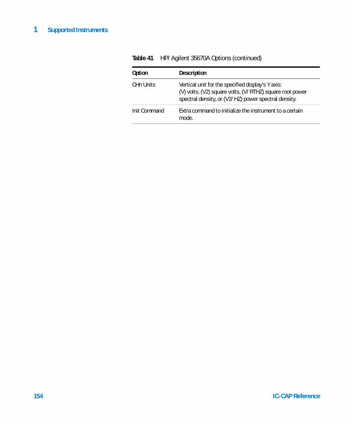
154
1 Supported Instruments
CHn Units Vertical unit for the specified display’s Y axis: (V) volts, (V2) square volts, (V/RTHZ) square root power spectral density, or (V2/HZ) power spectral density.
Init Command Extra command to initialize the instrument to a certain mode.
Table 41 HP/Agilent 35670A Options (continued)
Option Description
IC-CAP Reference

Agilent 85190A IC-CAP 2008Reference
2Drivers
Prober Drivers 156
Prober Driver Test Program 166
Matrix Drivers 168
Using IC-CAP with the HP 5250A Matrix Driver 180
Using IC-CAP with HP 4062UX and Prober/Matrix Drivers 187
Adding Instrument Drivers to IC-CAP 191
Class Hierarchy for User-Contributed Drivers 228
Order in Which User-Supplied Functions are Called 231
Handling Signals and Exceptions 238
This chapter describes prober and matrix driver functions, prober settings and commands, the prober driver test program, and using OMI to add drivers.
155Agilent Technologies

2 Drivers
Prober Drivers
156
A prober driver is a set of USERC functions designed to control an IC wafer prober from an IC-CAP macro program. There are 3 types of probers (an initial call declares which type is in use) with these symbolic names:
• EG1034X (ElectroGlas 1034X), EG2001X (ElectroGlas 2001X)
• APM3000A (and APM6000A and APM7000A) (TSK APM models)
• SUMMIT10K (Cascade SUMMIT 10000)
These probers share the same driver functions. External user functions and internal design functions, as well as prober settings and commands, are described in this section.
Additional TIS prober drivers required the renaming of native IC-CAP prober functions from prober_xxxx() to icprober_xxxx(). This only affects systems where the prober.c file has been customized in the OMI environment, and will not affect previously-written macros. See the Readme file in $ICCAP_ROOT/src/README for information about these functions.
To provide easier manipulation of a raw GPIB device file, IC-CAP offers a set of low-level I/O functions named ice_hpib_xxxx. The declarations of these functions are found in icedil.h; their definitions are in icedil.c. Both files are provided as C source files. For more information on these I/O functions, see Appendix I, “icedil Functions” in online help. Driver functions are contained in the directory $ICCAP_ROOT/src in the files shown in the following table.
Table 42 Prober Driver Source Files
File Name Description
prober.h Prober call prototypes for userc.c
prober.c Actual code for each prober function
icedil.h Low level I/O call prototypes for prober.c
IC-CAP Reference

Drivers 2
IC-CAP Reference
A custom driver can be added by editing prober.c in $ICCAP_ROOT/src and generating a new shared library file, libicuserc.<ext> (where ext is a platform-specific extension) because all prober drivers are written in C and treated as library functions.
• For information on libicuserc, refer to “Creating a New Shared Library” on page 203.
• For details regarding adding library functions, refer to “Creating C Language Functions in IC-CAP" in the IC-CAP User’s Guide.
Source code is provided with this open interface. Recompilation and relinking are necessary if this driver is user-modified.
icedil.c Actual code for each ice_hpib_xxxx call
testprob.c Small interactive program to test the driver
run_testprob Properly sets your shared library lookup path and runs ./testprob if it exists, otherwise it runs $ICCAP_ROOT/bin/testprob. ICCAP_ROOT must be properly set in your environment for run_testprob to work.
Table 42 Prober Driver Source Files
File Name Description
External Prober User Functions
This section describes the external user functions.
Prober_debug This function takes 2 arguments and sets the internal flags. The first argument defines the debug flag; when it is 1, all debugging information is displayed in the Status window. The second argument defines the stop flag; when it is 1, the Macro execution stops when an error is detected. After Prober_init(), the debug flag is off (0) and the stop flag is on (1). This function does not exist in TIS. This function always returns 0. An example call is:x = Prober_debug (1, 0);
157

158
2 Drivers
Every function looks at this internal debug flag and prints out any GPIB commands it is going to send, or a string it just received from the prober.
Prober_init This function must be called before any other prober calls are made in a Macro program. This function takes a GPIB address of the prober, flat orientation, prober type name, and a raw GPIB interface name to which the prober is connected. The flat orientation is usually 0, 90, 180, or 270. The function returns 0 when prober initialization is successful and −1 when it fails. The following table lists the GPIB configuration recommended for HP 4062UX.
NOTE A raw GPIB interface name is different for each platform. Refer to the following table for this name. A separate GPIB interface may be necessary if the given prober does not conform to IEEE 488 standard.
For a Sun SPARC computer, use the following call because a National Instruments GPIB card has this name by default:x = Prober_init (1, 0, “EG1034X”, “/dev/gpib0”);
For an HP 700 Series computer, use the following call because it involves a symbolic name rather than a GPIB interface filename:x = Prober_init (1, 0, “EG1034X”, “hpib”);
This function also checks the prober type and sets the internal prober type flag for subsequent driver calls. It closes its private unit descriptor from any previous prober access, opens the given GPIB interface file and keeps a new entity id. It then calls an appropriate subfunction, which does the prober-dependent initialization.
Table 43 Standard HP 4062UX Configuration
Select Code Devices
7 or 27 Instruments and Switching Matrix
25 Wafer Prober
IC-CAP Reference

Drivers 2
IC-CAP Reference
Prober_reset This function takes no arguments and sets the prober to Local mode. It returns 0 when successful and 1 when it fails. This function is not available for EG1034X (for which it is a no-operation). An example call is:x = Prober_reset ();
This function clears the interface file and sends a selected device clear command to the prober.
Prober_status This function takes no arguments and returns 3 Real values in 1 array. The first element of the array indicates whether the prober is Remote (1) or Local (0). The second element indicates whether the edge contact is detected (1) or not (0). The last element indicates whether the Cassette is empty (1) or not (0). An example call is:status = Prober_status ();if (status[0] == 1) then ...
This function sends a query command to the prober and receives information about Remote/Local state as well as the edge sensor output. The Cassette Empty error is detected in the function Phome and referred by this function, which keeps these states and returns them back in an array of Real values.
Pdown This function takes no arguments and lowers the chuck of the wafer prober. It returns 0 when successful and −1 when it fails. An example call is: x = Pdown ();
Phome This function takes no arguments and performs several tasks depending on the prober type. It returns 0 when successful and −1 when it fails. When it detects a Cassette Empty error, it returns 1. An example call is: x = Phome ();
This function calls a subfunction based on the prober type. A subfunction actually does the prober-dependent operation appropriate for Phome.
NOTE Set the SUMMIT 10000 prober to Remote manually after this function to move the chuck to its Load position and turn the mode to Manual for wafer alignment.
159
160
2 Drivers
Pimove Like Pmove, this function takes 2 arguments and moves the chuck relative to the current position. It returns 0 when successful and −1 when it fails. An example call is:x = Pimove (1, 0);
Pink This function takes 1 argument and triggers the specified inker. It returns 0 when successful or −1 when it fails. EG1034X and SUMMIT10K probers do not support an inker, so this function is a no-operation for them. An example call is:x = Pink (1);
Pmove This function takes 2 arguments and moves the chuck to the specified absolute coordinates established by Pscale and Porig. The first argument specifies the new X position and the second specifies the new Y position. It returns 0 when successful and −1 when it fails. An example call is:x = Pmove (2, 4);
This function calculates how many machine units the chuck must move relative to the current position, and sends an appropriate GPIB command to move the chuck. It also updates its internal variables to keep track of the position.
Porig This function takes 2 numbers and defines these numbers as X and Y coordinates of the current chuck position. This function must be called before any Pmove or Pimove functions. It always returns 0. An example call is:x = Porig (0, 0);
This function stores the given numbers in its private variables.
Ppos This function takes no arguments and returns 2 Real values in an array, indicating the current die X and Y position being probed. The first element of the array is the X coordinate and the second is the Y coordinate. An example call is:position = Ppos ();print “X = “; position[0], “Y = “; position[1];
This function copies its private variables (which indicate the current position) and returns them.
IC-CAP Reference

Drivers 2
IC-CAP Reference
Pscale This function takes the die X and Y dimensions in micrometers. These numbers are later used in Pmove, Porig, and Pimove functions. It always returns 0. An example call is:x = Pscale (5000, 5000);
This function stores the given numbers in its private variables.
Pup This function takes no arguments and raises the chuck of the wafer prober so that probe pins come in contact with the wafer. It returns 0 when successful and −1 when it fails. An example call is:x = Pup ();
Internal Prober Functions
Several internal functions support the user functions to customize the prober driver. For each algorithm, refer to the prober.c source file.
prober_get_err This function takes 1 argument and calls a subfunction depending on the prober type. Each subfunction reads any error status from the prober. If it encounters an unknown error, it prints out the given number with an error message to the Status window. It always returns 0. An example call is:ret = prober_get_err(n);
prober_get_srq This function takes no arguments and returns 0 (no SRQ) or 1 (SRQ) depending on the SRQ line of the device file. An example call is:ret = prober_get_srq();
prober_message This function takes 1 argument, a pointer to a string, and prints an error message to the Status window such as <name>: unknown prober type, where <name> is replaced with the given string. An example call is:ret = prober_message(“Prober_reset”);
prober_precheck This function takes no arguments and checks prober state such as Remote/Local and SRQ. It returns 0 when successful and −1 when it fails. An example call is:ret = prober_precheck();
161

162
2 Drivers
prober_response This function takes 1 argument that is either a pointer to a character array or null. It calls a subfunction depending on the prober type and each subfunction reads any status information from the prober. Internal flags are set according to the status and any errors are reported. It returns 0 if there is no error. If a non-null pointer is given, a received string from the prober is returned using this pointer. An example call is:char buffer[PSIZE];ret = prober_response(buffer);
prober_spoll This function takes no arguments and performs serial polls in a prober-dependent way that may be different from the standard IEEE 488 implementation. It returns a status byte from the prober. An example call is: ret = prober_spoll();
prober_wait_srq This function takes 1 argument that is a timeout value in seconds, and waits for SRQ to be asserted. It returns 0 when SRQ is detected and −1 when a timeout or error occurs. An example call is:ret = prober_wait_srq(60.0); /* 60 sec */
Prober Settings and Commands
This section describes the correct IC-CAP wafer prober settings and their associated GPIB commands.
EG1034X
This simple manual prober uses 2 settings. (Note that IC-CAP uses SRQ whereas HP 4062UX does not.)
• GPIB Address: Any
• SRQ Switch: Enabled
The following table lists the EG1034X GPIB commands. (Note that IC-CAP uses the MM command to move the chuck; HP 4062UX uses the MO commands for the EG1034X.)
IC-CAP Reference

Drivers 2
IC-CAP Reference
EG2001X
This driver is tested with a prober software version called AC. The parameters listed in the following table must be set to control this prober. Note that the I/O PROTOCOL is different from the one for HP 4062UX. The Die Size is optional, but is included because IC-CAP does not set the size for manual operations.
The following table lists the EG2001X GPIB commands. Note that Chuck Home uses both UL and LO commands (HP 4062UX uses LO).
Table 44 EG1034X GPIB Commands
Item Command Reply Item Command Reply
Move Chuck MM MC Chuck Home HO MC
Chuck Up ZU MC Chuck Status ?S SZ...
Chuck Down ZD MC
Table 45 EG2001X Settings
Parameter Value Parameter Value
METRIC/ENGLISH METRIC AUTO LOAD ENB if available
DIE X and Y SIZE Any AUTO ALIGN ENB if available
AUTO PROBER PAT. EXTERNAL AUTO PROFILE ENB if available
AUTO DIAMETER ENB MF/MC on X-Y ENB
Z-TRAVELING MODE EDGE-SEN MF/MC on Z DIS
I/O PROTOCOL ENHANCED MF/MC on OPT. ENB
I/O PORT GPIB-SP MF/MC on others DIS
GPIB ADDRESS Any
SRQ SWITCH ENB
163

164
2 Drivers
APM3000A, APM6000A, APM7000A
This prober uses the following settings:
• GPIB Address: Any
• Mode Switches: 3-4 OFF, 3-5 ON, 23-4 ON
The following table lists the commands.
SUMMIT10K
This driver waits for an SRQ for an operation completed. With Summit Software version 2.10, the F10 key enables Remote mode. This prober uses the following settings.
• COMMUNICATION PROTOCOL: GPIB
• COMMAND SET: native
• DISP REMOTE CMDS: off
• BUS ADDRESS: any
• TIMEOUT: 30.0
• CONTROL MODE: remote
Table 46 EG2001X GPIB Commands
Item Command Reply Item Command Reply
Move Chuck MM MC or MF Auto Profile PZ MC or MF
Chuck Up ZU Auto Align AA MC or MF
Chuck Down ZD Trigger Inker IK MC or MF
Chuck Home UL/LO MC or MF Chuck Status ?S SZ...
Table 47 APM3000A, APM6000A, and APM7000ACommands
Item Command Reply Item Command Reply
Move Chuck A 65 CPU Halt T
Chuck Up Z 67 or 73 Trigger Inker M 69
Chuck Down D 68 Chuck Home L 70 or 76
IC-CAP Reference

Drivers 2
IC-CAP Reference
SUSS PA 150, PA 200
The SUSS ProberBench Interface developed by Karl Suss for IC-CAP is provided as a convenience, but is not supported by Agilent Technologies. The prober driver supports all functions described in “External Prober User Functions” on page 157 and “Internal Prober Functions” on page 161 except prober_spoll(), prober_get_srq(), and prober_wait_srq(). In addition to these IC-CAP functions, you can use the complete ProberBench command set (150 functions) to enhance operation. For information on these functions, refer to the ProberBench User Manual. For information on writing macros to control the prober, refer to “Writing a Macro” on page 187.
The SUSS PA 150 and PA 200 Semiautomatic Probers utilize a Microsoft Windows-based user interface running on an IBM-compatible PC. The IC-CAP environment communicates with the prober via a macro over the IEEE 488 bus.
The required PC IEEE488 control hardware is: IOtech Personal488/AT.
The PC configuration must use the following values for the settings shown; all other settings use default values:
Interface Type: GP488B
Name: IEEE
IEEE Bus Address: 22
System Controller: Off
Time-out (ms): 3000
Interface Bus Address: 02E1
DMA Channel: None
Interrupt: None
165

2 Drivers
Prober Driver Test Program
166
This section describes the prober test program testprob, which is provided with C source code. This program runs independently from IC-CAP and interactively calls driver functions to test an Agilent-supplied or a custom driver.
The file for this program is located in $ICCAP_ROOT/src and is called testprob.c. It includes the test program main. The Makefile offers an option to build this test program. This program is linked with prober.o, iceswn.o, icedil.o, a GPIB library to exercise both prober and switching matrix drivers. If testprob has been rebuilt with a custom driver, use an absolute path to specify the new testprob because $ICCAP_ROOT/bin has another, original testprob executable.
The testprob executable is an interactive program that gets user input from its stdin and calls an appropriate driver function, then prints out the return value(s) of the driver function to the Status window.
The run_testprob script properly sets your shared library lookup path and runs ./testprob if it exists, otherwise it runs $ICCAP_ROOT/bin/testprob. Therefore, you should use the run_testprob script to run testprob. Make sure $ICCAP_ROOT is properly set in your environment, then type run_testprob.
An actual prober (matrix) must be connected to a raw GPIB device file in order to perform driver (matrix) tests. Off-line testing is not available with this program.
This program expects to see a function name and its arguments as if they appeared in an IC-CAP Macro program. However an argument list cannot include another function, that is, nesting is not allowed.
A command example is:Prober_init(1, 0, “EG1034X”, “hpib”)
IC-CAP Reference

Drivers 2
IC-CAP Reference
The currently supported functions are shown next.
Connect Prober_debug
FNPort Prober_init
Pdown Prober_reset
Phome Prober_status
Pimove Pscale
Pink Pup
Pmove SWM_debug
Porig SWM_init
Ppos Wait
NOTE Any line starting with # is treated as a comment and is ignored. A blank line is skipped (this is helpful when a file is used to supply input to this program).
Because this test program is not a real Macro interpreter, it has the following restrictions:• No control constructs
• No variables
• No nesting of functions
• No function library other than the prober and matrix driver
• No capability to execute IC-CAP Macro programs.
Because nesting is not supported, the Connect function needs a port address such as 32701 instead of FNPort(1). Refer to the HP 4062UX Programming Reference for more information about port addresses.
167

2 Drivers
Matrix Drivers
168
A matrix driver is a set of USERC functions designed to control the switching matrices through an HP 4084 controller from an IC-CAP Macro program. The matrix driver supports the matrices listed in the following table.
External user functions and internal design functions are described in this section. They are designed to be compatible with HP 4062UX TIS where possible.
Source files for this matrix driver are iceswm.h and iceswm.c. The header file iceswm.h is included in userc.c so that the function names can appear in the Function List of IC-CAP.
Source code is provided with this open interface.
Table 48 Types of Matrix Drivers
Matrix Controller Pins Device
HP 4085A HP 4084A 48 HP 4062A and HP 4062B
HP 4085B HP 4084B 48 HP 4062C and HP 4062UX
HP 4089A HP 4084B 96 same as above, with 2 controllers
External Matrix Driver User Functions
This section describes the matrix driver external user functions.
SWM_debug This function takes 1 argument and sets the internal debug flag. When the argument is 1, debugging information is printed out to the Status window; when the argument is 0, printing is turned off. It always returns 0. This function does not exist in TIS. An example call is:x = SWM_debug(1)
Every function looks at this flag and prints out any GPIB commands it is going to send, or a string it just received from a matrix controller.
IC-CAP Reference

Drivers 2
IC-CAP Reference
SWM_init This function takes 2 GPIB addresses, a matrix name, and a raw GPIB interface name to which the matrix is connected. The first GPIB address is for the block 1 (usually 19) and the second is for the block 2 (22). However, a different address can be assigned for each matrix controller. For the HP 4085A and HP 4085B (both 48-pin systems), the second address is used as the controller address, and the first address is ignored. It returns 0 when successful and −1 when it fails. This function does not exist in TIS. An example call is: x = SWM_init (19, 22, “HP4089A”, “hpib”); ! for 96-pin
or x = SWM_init (0, 22, “HP4085B”, “hpib”); ! for 48-pin
This function checks the matrix type and sets the internal type flag for subsequent matrix calls. It closes its private entity id from a previous matrix access (when it exists), and opens the given raw GPIB device file. Then it calls an internal function swm_init_unit to reset a controller. This clears all pins and ports.
Connect This function takes a port address and a pin number and connects the given port to the pin. The port address is either 0 or from 32701 to 32711, inclusive. The pin number is 0 or from 1 to 48/96 inclusive. When a pin card does not exist for the given pin number, it gives an error message and aborts the Macro execution.
An example call is: x = Connect(32701, 25);
This function sends GPIB commands to the matrix controller and either connects or disconnects the specified port and pin. The following table lists argument combinations.
Table 49 Argument Combinations
Port Address Pin Number Description
0 0 Disconnect all pins from all ports.
0 X Disconnect pin X from its connected port.
X 0 Disconnect all pins connected to port X.
169

170
2 Drivers
As in TIS, multiple pins can be connected to 1 port by calling this function several times. Pin numbers 1 through 48 belong to block 1; pin numbers 49 through 96 belong to block 2. When a 96-pin matrix is used, do not connect block 1 and block 2 pins to 1 single port. Because this function does not include switching delay, allow enough wait time before and after measurement to prevent relay damage. Virtual Front Panel (VFP) is not supported.
FNPort This function takes a port number and returns a port address for Connect. This allows compatibility with the HP 4062UX. An example call is:port = FNPort(1);
Wait This function takes a wait time, in seconds, to give a necessary delay to wait until SMU outputs become zero for dry switching. This function does not exist in TIS. It returns 0 when successful or −1 when it fails. An example call is:x = Wait (0.1) ! 100ms delay;
X Y Connect port X to pin Y.
Table 49 Argument Combinations
Port Address Pin Number Description
Internal Matrix Driver Functions
The internal functions described next support the user functions. Refer to the source file for each algorithm.
swm_connect_pin This function takes a GPIB address of a controller, a port number, and a pin number. It sends a Pin Connect command to the controller, and is called from swm_connect (Connect) to actually perform the pin connection and disconnection.
swm_connect_port This function takes a GPIB address and a port number to send a Port Connect command to the controller, which manages input relays of an HP 4089A matrix.
IC-CAP Reference

Drivers 2
IC-CAP Reference
swm_cut_port_pin This function takes a GPIB address and a pin number to cut the pin connection when a 96-pin matrix is used. It also checks if the port to which the pin was connected can be turned off; if it can (both Force and Guard are off), it turns off this port.
NOTE When a switching matrix controller shares a single GPIB with other instruments, set the system variable INST_START_ADDR to a value greater than the matrix controller’s GPIB address. This prevents IC-CAP from accessing the controller while performing Rebuild (instrument list).
swm_init_unit This function takes a file designator (or eid, a small integer usually obtained by calling the open system function) and a GPIB address of a matrix controller. It is called from swm_init to initialize a controller and clear all pins and ports for which the controller is responsible.
swm_parse_err This function takes a status byte sent from a matrix controller and determines the cause of an SRQ. If there is no error, it returns 0 to allow the caller to keep running. If there is an error, it returns −1 to abort the execution of the caller.
swm_release_port This function takes a GPIB address and a port number to send a Port Disconnect command to the controller only when a 96-pin matrix is used. Because block 1 and block 2 pins should not be connected to a single port, a disconnect request such as Connect(32701, 0) not only cuts the connection between a port and a pin, but also disconnects the input relays of the port.
171

2 Drivers
Using IC-CAP with B2200A/B2201 Low-Leakage Mainframe Driver
172
This section describes the transforms implemented for the B2200A/B2201 Low-Leakage Mainframe Driver.
List of the transforms:
• B2200_bias_card_enable
• B2200_bias_ch_enable
• B2200_bias_enable
• B2200_bias_init
• B2200_close_interface
• B2200_connect
• B2200_couple_enable
• B2200_couple_setup
• B2200_debug
• B2200_disconnect_card
• B2200_GPIB_handler
• B2200_ground_card_enable
• B2200_ground_enable
• B2200_ground_init
• B2200_ground_outch_enable
• B2200_ground_unused_inputs
• B2200_init
• B2200_open_interface
The following sections describe these transforms. For more details about the Agilent B2200A/B2201A, see its User Guide.
Utility Functions
B2200_debug When set to 1, prints out all command strings sent to the instrument. This flag is common to all B2200A’s on the bus, regardless of their GPIB address.B2200_debug(<flag>)
IC-CAP Reference

Drivers 2
IC-CAP Reference
where:
<flag> is "1", "0", "Yes", or "No".
B2200_close_interface Closes the current interface, which was opened by calling B2200_open_interface().
B2200_GPIB_handler Returns -1 if the interface has not been initialized (invalid handler). Returns a positive integer (handler) if the interface has been opened.
Returns the current interface handler. The function is provided as a utility function, which enables you to write advanced PEL code to write and read data to the B2200A using the HPIB_write and HPIB_read functions. Initializing the handler using B2200_open_interface enables you to use B2200A's built-in driver functions as well as writing PEL code to support other features that are not currently supported by the built-in functions, all in the same PEL code.
Initialization and General ConfigurationB2200_open_interface Opens and initializes the GPIB interface and must be run first in the PEL program. The interface handler is saved in a static variable so that the interface will be shared by all the other B2200's function calls. You can drive multiple B2200 instruments as long as they are on the same interface bus (obviously, they must have different addresses).B2200_open_interface(<Interface Name>)
where:
<Interface Name> is the name of the GPIB interface.
B2200_init Must be run first in the PEL program to initialize the instrument and set the configuration mode. When the instrument is in AUTO configuration mode and multiple plug-in cards are installed in the B2200 slots from
173

174
2 Drivers
slot 1 continuously, the installed cards are then treated as one card (numbered 0). This function resets all the settings to factory default before setting the configuration mode.
This function also sets the default connection rule for the specified card. When the connection rule is FREE (default mode), each input port can be connected to multiple output ports and each output port can be connected to multiple input ports. When the connection is SINGLE, each input port can be connected to only one output. Connection sequence specifies the open/close sequence of the relays when changing from an existing connection to a new connection.B2200_init(<addr>,<cardNumber>,<config>,<connectionRule>, <connectionSequence>)
where:
<addr> is the GPIB address of the Mainframe (must be a positive number from 1 to 30).
<cardNumber> is 0(auto), 1, 2, 3, or 4.
<config> is "AUTO" or "NORMAL" (string input).
<connectionRule> is "FREE" or "SINGLE".
<connectionSequence> is "NSEQ", "BBM", or "MBBR".
• NSEQ (No SEQuence): Disconnect old route, connect new route.
• BBM (Break Before Make): Disconnect old route, wait, connect new route.
• MBBR (Make Before BReak): Connect new route, wait, disconnect old route.
Transforms Governing the Bias Mode
B2200_bias_init Selects the Input Bias Port for the specified card. The Input Bias Port is the dedicated bias port.B2200_bias_init(<addr>, <CardNumber>, <InputBiasPort>)
where:
<addr> is the GPIB address of the Mainframe (must be a positive number from 1 to 30).
IC-CAP Reference

Drivers 2
IC-CAP Reference
<CardNumber> is 0(auto), 1, 2, 3, or 4.
<InputBiasPort> is 1 to 14 (numeric input) or −1 to disable bias port.
B2200_bias_ch_enable This function bias-enables specific output ports in the channel list for the specified card. The input ports specified in the channel list are ignored since the input port is always the Bias Input Port. By default, all the outputs are bias-enabled after a reset.B2200_bias_ch_enable(<addr>,<CardNumber>,<State>,<Channel list>)
where:
<addr> is the GPIB address of the Mainframe (must be a positive number from 1 to 30).
<CardNumber> is 0(auto), 1, 2, 3, or 4.
<State> is the output port's state (allowed values are "ENABLE", "DISABLE", "E", or "D")
<Channel list> is the list of channels, known as connection routes. Example channel list: (@10102, 10203, 10305:10307)
B2200_bias_card_enable This function bias-enables all the output ports of the specified card. By default, all ports are bias-enabled after a reset.B2200_bias_card_enable(<addr>, <CardNumber>, <CardState>)
where:
<addr> is the GPIB address of the Mainframe (must be a positive number from 1 to 30).
<CardNumber> is 0(auto), 1, 2, 3, or 4.
<CardState> is the card output port's state (allowed values are "ENABLE", "DISABLE", "E", or "D").
B2200_bias_enable Enables the bias mode for the specified card once Input Bias Port and Enabled Output ports are specified. When Bias Mode is ON, the Input Bias Port is connected to all Bias Enabled output ports that are not
175

176
2 Drivers
connected to any other input ports. Bias Disabled output ports are never connected to an Input Bias Port when Bias Mode is ON.
If another input port is disconnected from a bias enabled output port, this port is automatically connected to the Input Bias Port.
If another input port is connected to a Bias Enabled output port, the output port is automatically disconnected from the Bias Input Port. When Bias Mode is OFF, the Input Bias Port is the same as the other ports.B2200_bias_enable(<addr>, <CardNumber>, <mode>)
where:
<addr> is the GPIB address of the Mainframe (must be a positive number from 1 to 30).
<CardNumber> is 0(auto), 1, 2, 3, or 4.
<mode> is "On", "Off", "1", or "0".
Transforms Governing the Ground Mode
B2200_ground_init Selects the input Ground Port for the specified card. For each card, you can specify the same or a different Ground Port. By default, the input Ground Port is port 12. The ground port should be connected to 0 V output voltage. See the Agilent B2200 User's Guide for details.B2200_ground_init(<addr>,<CardNumber>,<InputGroundPort>)
where:
<addr> is the GPIB address of the Mainframe (must be a positive number from 1 to 30).
<CardNumber> is 0(auto), 1, 2, 3, or 4.
<InputGroundPort> is 1 to 14 (numeric input) or −1 to disable ground port.
B2200_ground_outch_enable Ground-enables or ground-disables output ports. When Ground Mode is turned ON, the ground-enabled output ports that have not been
IC-CAP Reference

Drivers 2
IC-CAP Reference
connected to any other input port are connected to the input ground port. The input ports specified in channel lists are ignored since the input port is always the Input Ground Port. By default, all the outputs are ground-disabled after a reset.B2200_ground _outch_enable(<addr>,<CardNumber>,<State>, <Channel list>)
where:
<addr> is the GPIB address of the Mainframe (must be a positive number from 1 to 30).
<CardNumber> is 0(auto), 1, 2, 3, or 4.
<State> is the port's state (allowed values are "ENABLE", "DISABLE", "E", or "D").
<Channel list> is the list of channels, known as connection routes. Example channel list: (@10102, 10203, 10305:10307)
B2200_ground_unused_inputs Specifies the ground-enabled (or unused) input ports for the specified card. When Ground Mode is turned ON, the ground-enabled input ports that have not been connected to any other port are connected to the input Ground Port. By default, all the inputs are ground-disabled after a reset.B2200_ground _unused_inputs(<addr>,<CardNumber>,<Input Channels>)
where:
<addr> is the GPIB address of the Mainframe (must be a positive number from 1 to 30).
<CardNumber> is 0(auto), 1, 2, 3, 4.
<Input Channels> is the list of input channels (e.g., "1, 2, 5"). Only input ports 1 to 8 can be defined as unused (these are the input Kelvin Ports).
B2200_ground_card_enable Enables ground-enabling for all the output ports of the specified card. By default, all ports are ground-disabled.B2200_ground_card_enable(<addr>,<CardNumber>,<CardState>)
where:
177

178
2 Drivers
<addr> is the GPIB address of the Mainframe (must be a positive number from 1 to 30).
<CardNumber> is 0(auto), 1, 2, 3, or 4.
<CardState> is the card output port's state (allowed values are "ENABLE", "DISABLE", "E", or "D").
B2200_ground_enable Enables the bias mode for the specified card. When Ground Mode is turned ON, the Input Ground Port (default is 12) is connected to all the Ground Enabled input/output ports that have not been connected to any other port. At Reset, Ground Mode is OFF. Ground Mode cannot be turned ON when Bias Mode is ON.
See the Agilent B2200 User's Guide for additional comments and restrictions.B2200_ground_enable(<addr>, <CardNumber>, <mode>)
where:
<addr> is the GPIB address of the Mainframe (must be a positive number from 1 to 30).
<CardNumber> is 0(auto), 1, 2, 3, 4.
<mode> is "On", "Off", "1", or "0".
Transforms Governing the Couple Mode
B2200_couple_enable Use this function to enable or disable Couple Port mode. Couple Port mode allows synchronized connection of two adjacent input ports to two adjacent output ports.B2200_couple_enable(<addr>, <CardNumber>, <Mode>)
where:
<addr> is the GPIB address of the Mainframe (must be a positive number from 1 to 30).
<CardNumber> is 0(auto), 1, 2, 3, or 4.
<mode> is "On", "Off", "1", or "0".
IC-CAP Reference

Drivers 2
IC-CAP Reference
B2200_couple_setup Selects the couple ports for Kelvin connections. At Reset, no input ports are coupled.B2200_couple_setup(<addr>,<CardNumber>,<ListOfCoupledPorts>)
where:
<addr> is the GPIB address of the Mainframe (must be a positive number from 1 to 30).
<CardNumber> is 0(auto), 1, 2, 3, or 4.
<ListOfCoupledPorts> is the list of odd number input channels (e.g., "1, 3, 5" means coupled ports are 1-2, 3-4, 5-6).
Transforms Governing the Switching
B2200_connect Connects or disconnects specified channels. Bias Mode and coupling Mode are also taken into account when a channel is closed or opened.
For example, in the list (@10102, 10203:10205), the following channels are connected or disconnected on card 1. Input port 1 to output port 2. Input port 2 to output port 3 and 5.B2200_connect(<addr>,<Connect/Disconnect>,<ChannelList>)
where:
<addr> is the GPIB address of the Mainframe (must be a positive number from 1 to 30).
<Connect/Disconnect> is C or D.
<ChannelList> is the list of connections to close.
B2200_disconnect_card Opens all relays or channels in the specified cards.B2200_disconnect_card(<addr>, <CardNumber>)
where:
<addr> is the GPIB address of the Mainframe (must be a positive number from 1 to 30).
<CardNumber> is 0(auto), 1, 2, 3, or 4.
179

2 Drivers
Using IC-CAP with the HP 5250A Matrix Driver
180
This section describes the transforms implemented for the HP 5250A Switching Matrix.
NOTE The old switching box transforms that were implemented for the HP 40XX series are not compatible with the new ones. The instruments have different commands for switching and the 5250A has new features such as BIAS and COUPLE modes, which were not available for the old 40XX series.
List of the transforms:
• HP5250_debug
• HP5250_init
• HP5250_card_config
• HP5250_bias_init
• HP5250_bias_card
• HP5250_bias_channel
• HP5250_bias_setmode
• HP5250_couple_setup
• HP5250_couple_enable
• HP5250_connect
• HP5250_disconnect_card
• HP5250_compensate_cap
• HP5250_show()
The following sections describe these transforms. For more details about the HP 5250A, see its User Guide.
IC-CAP Reference
Drivers 2
Utility Functions
IC-CAP Reference
HP5250_debug This transform is only for debugging. When the debug flag is set to 1, all the functions print out all the command strings that are sent to the instruments. Set flag using the values 1 or 0, or use YES or NO. HP5250_debug(<flag>)
HP5250_compensate_cap This transform is the equivalent IC-CAP C routine for the HP BASIC capacitance compensation routine called Ccompen_5250 supplied with the HP 5250A. It returns a 2 by 1 matrix (2 rows, 1 column) defined as follows:
• output.11 represents compensated capacitance data [F].
• output.21 represents compensated conductance data [S].HP5250_compensate_cap (RawCap, RawCond, Freq, HPTriaxLenght,UserTriaxLenghtHigh, UserTriaxLenghtLow, UserCoaxLenghtHigh,UserCoaxLenghtLow)
where:
RawCap is Input Dataset containing raw capacitance data [F]
RawCond is the Input Dataset containing raw conductance data [S]
Freq is the measured frequency [Hz]
HPTriaxLenght is the HP Triax Cable Length [m]
UserTriaxLenghtHighis the user Triax Cable Length (High) [m]
UserTriaxLenghtLow is the user Triax Cable Length (Low) [m]
UserCoaxLenghtHigh is the user Coax Cable Length (High) [m]
UserCoaxLenghtLow is the user Coax Cable Length (Low) [m]
181

182
2 Drivers
HP5250_show() This transform has no inputs. It returns to the standard output (screen or file) the following data about the instrument status:
• Instrument Name
• Instrument Configuration (AUTO/NORMAL).
The following information is output for each card installed in the instrument (card 0 if the instrument is in auto configuration mode):
• Connection mode
• Connection sequence
• Input Bias Port
• Enabled Output Bias Ports
• Bias Sate (ON/OFF)
• Coupled Input Ports (only lower number is listed, e.g., “3,5” means ports 3 and 4 are coupled
• Couple Port Mode (ON/OFF)
• Connection Matrix Inputs(10)xOutputs(12,24,36, or48). The following table shows an output example of the Channel Matrix State where Card 1 is a 10x12 matrix switch. A “1” in a matrix cell means the connection is closed.
Output Ports
1 2 3 4 5 6 7 8 9 10 11 12
1 0 0 0 1 0 0 0 0 0 0 0 0
2 1 1 1 1 1 0 0 0 0 0 0 0
3 0 1 0 0 0 0 0 0 0 0 0 0
Input 4 0 0 0 0 0 0 0 0 0 0 0 0
Ports 5 0 0 0 0 0 0 0 0 0 0 0 0
6 0 0 0 0 0 0 0 0 0 0 0 0
7 0 0 0 0 0 0 0 0 0 0 0 0
8 0 0 0 0 0 0 0 0 0 0 0 0
9 0 0 0 0 0 0 0 0 0 0 0 0
10 0 0 0 0 0 0 0 0 0 0 0 0
IC-CAP Reference

Drivers 2
Initialization and General Configuration
IC-CAP Reference
HP5250_init This transform must be run first to initialize the instrument with the address and interface. Using this transform the configuration mode can be set to AUTO. When the instrument is in AUTO configuration mode the same type of card must be installed in the HP 5250 slots from slot 1 continuously. The installed cards are then treated as 1 card (numbered 0).HP5250_init (BusAddress, "Interface", "Configuration")
where
BusAddress is interface bus address (default is 22)
"Interface" is interface name (default is hpib)
"Configuration" is AUTO/NORMAL A/N (default is NORMAL)
HP5250_card_config This transform is used to change the default configuration for the specified card. When the connection rule is FREE (default mode), each input port can be connected to multiple output ports and each output port can be connected to multiple input ports. When the connection is SINGLE, each input port can be connected to only 1 output. Connection sequence specifies the open/close sequence of the relays when changing from an existing connection to a new connection.HP5250_card_config (CardNumber, "ConnRule", "ConnSequence")
where
CardNumber specifies the card (0 for AUTO configuration mode)
"ConnRule" is FREE/SINGLE (default is FREE)
"ConnSequence" is NSEQ/BBM/MBBR (default is BBM)
• NSEQ (No SEQuence): Disconnect old route, connect new route.
• BBM (Break Before Make): Disconnect old route, wait, connect new route.
183

184
2 Drivers
• MBBR (Make Before BReak): Connect new route, wait, disconnect old route.
Transforms Governing the Bias Mode
HP5250_bias_init This transform selects the bias port. When using the HP/Agilent E5255A card, the Input Bias Port is the dedicated bias port; however, for the HP/Agilent E5252A the Input Bias Port must be selected using this function.HP5250_bias_init(CardNumber, InputBiasPort)
where
Card Number specifies the card (allowed values 0-4, 0 = auto configuration mode)
InputBiasPort specifies the input bias port number (allowed values are 1-10)
HP5250_bias_card This transform bias-enables all the output ports for the specified card.HP5250_bias_card(CardNumber, "CardState")
where
CardNumber specifies the card (allowed values 0-4, 0 = auto configuration mode)
"CardState" is the card’s state (allowed values are ENABLE/DISABLE or E/D)
HP5250_bias_channel This transform bias-enables the specified output ports in the channel list. Note that the input ports are ignored since the input port is always the Bias Input Port.HP5250_bias_channel ("State", "Channel list")
where
"State" is the output port’s state (allowed values are ENABLE/DISABLE or E/D)
"Channel list" is the list of channels, known as connection routes
IC-CAP Reference

Drivers 2
IC-CAP Reference
Example channel list: (@10102, 10203, 10305:10307)
HP5250_bias_setmode This transform enables the bias mode for the specified card once Input Bias Port and Enabled Output ports have been specified.HP5250_bias_setmode (CardNumber, "BiasMode")
where
CardNumber specifies the card (allowed values 0-4, 0 = auto configuration mode)
"BiasMode" sets the bias mode on or off (allowed values are ON/OFF or 1/0)
When Bias Mode is ON, the Input Bias Port is connected to all the Bias Enabled output ports that are not connected to any other input ports. Bias Disabled output ports are never connected to an Input Bias Port when Bias Mode is ON.
• If another input port is disconnected from a bias enabled output port, this port is automatically connected to the Input Bias Port.
• If another input port is connected to a Bias Enabled output port, the output port is automatically disconnected from the Bias Input port.
When Bias Mode is OFF, the Input Bias Port is the same as the other ports.
Transforms Governing the Couple Mode
HP5250_couple_setup This transform sets up couple ports for making kelvin connections.HP5250_couple_setup (CardNumber, "InputPorts")
where
CardNumber specifies the card (allowed values 0-4, 0 = auto configuration mode)
"InputPorts" is the list of coupled ports
Example: In the list "1,3,5,7,9" the coupled ports are 1-2, 3-4, 5-6, 7-8, 9-10
185

186
2 Drivers
HP5250_couple_enable This transform enables couple port mode. Couple port allows synchronized connection of 2 adjacent input ports to 2 adjacent output ports.HP5250_couple_enable (CardNumber, "CoupleState")
where
CardNumber specifies the card (allowed values 0-4, 0 = auto configuration mode)
"CoupleState" is the coupled state (allowed values are ON/OFF or 1/0)
Transforms Governing the Switching
HP5250_connect This transform connects or disconnects specified channels. Note that Bias Mode and/or coupling Mode are also taken into account when a channel is closed or opened.HP5250_connect ("Action", "Channel list")
where
"Action" connects or disconnects channels (allowed values are C and D)
"Channel list" is the list of connection routes to be switched
Example: In the list (@10102, 10203:10205), the following channels are connected or disconnected on card 1:
Input port 1 to output port 2.
Input port 2 to output port 3, 4, and 5.
HP5250_disconnect_card This transform simply opens all relays or channels in the specified cards.HP5250_disconnect_card (CardNumber)
where
CardNumber specifies the card (allowed values 0-4, 0 = auto configuration mode)
IC-CAP Reference

Drivers 2
Using IC-CAP with HP 4062UX and Prober/Matrix Drivers
IC-CAP Reference
This section describes how to use HP 4062UX instruments and the prober/matrix from IC-CAP for wafer device characterization. Also included in this section is information about writing a macro, controlling the prober, and conditions of which to be aware.
While the HP 4062UX is an ideal instrument for performing device characterization with IC-CAP, it is necessary to understand IC-CAP, probers, matrices, and the instruments under control. IC-CAP is an independent program from HP 4062UX TIS or VFP. It is not necessary, and can be damaging, to run the START program before running IC-CAP. To run IC-CAP after running the START program, the HP/Agilent 4142B must first be reset manually.
After running the HP 4062UX START program, the HP/Agilent 4142B is put into its binary mode. Because IC-CAP assumes that all the instruments to which IC-CAP is connected accept ASCII commands, IC-CAP cannot recognize the 4142B. Reset the 4142B by sending a Device Clear or by turning the instrument off and on again. To send a Device Clear to the 4142B, use the IC-CAP GPIB analyzer (Tools menu):
1 In the Instrument Setup Window, choose Tools > Send Byte.
2 Enter the default value 20 and choose OK.
Writing a Macro
NOTE Execute the START program to run TIS applications on the HP 4062UX, similar to a normal power-up.
While instruments like the HP/Agilent 4142B and the HP 4280A are controlled by IC-CAP with Setup tables, both the wafer prober and the switching matrix must be controlled through macro programs using the Pxxxxx() and
187

188
2 Drivers
Connect() functions. The Setup table defines which measurement unit is going to force certain output. Users must perform the following actions:
1 Determine which matrix port needs to be connected to which matrix pin.
2 Write several Connect() functions in a macro program that invokes this Setup measurement with a iccap_func() statement.
The example shown in the following figure involves 4 SMUs of an HP/Agilent 4142B and measures Id_vs_Vg characteristics of an NMOS device on a wafer.
! Prober and Matrix Test Programx = swm_init(19, 22, "HP4085B", "/dev/ice_raw_hpib")x = connect(fnport(1), 15) ! SMU1 - Drainx = connect(fnport(2), 7) ! SMU2 - Gatex = connect(fnport(3), 8) ! SMU3 - Sourcex = connect(fnport(4), 6) ! SMU4 - Bulkx = prober_init(2, 0, "EG2001X", "/dev/ice_raw_hpib")!linput "Load Cassette and Press OK", msgstatus = prober_status() ! wait until Remotewhile (not status[0])
status = prober_status()endwhileiccap_func("/nmos2/large/idvg", "Display Plots")!x = pscale(8200, 8200) ! test chip die sizex = phome() ! goes to the first diewhile (x == 0)
x = porig(0, 0) ! first die coordinatesi = 0while (i < 5) ! test diagonal 5 dies
x = pdown()x = pmove(i, i)x = pup()printprint "Die Position X=";i;" Y=";i;iccap_func("/nmos2/large/idvg", "Measure")iccap_func("/nmos2/large/idvg", "Extract")i = i + 1
endwhilex = phome() ! load next wafer
endwhileif (x == 1) then linput "Cassette Empty. Test End.", msgx = connect(0, 0) ! disconnect matrix pins
Figure 4 Sample Wafer Test Program
IC-CAP Reference

Drivers 2
Prober Control
IC-CAP Reference
Prober control is determined by the number of test modules, which is either single or multiple per die.
With the Pxxxx functions, it is assumed that there is a single test module on each die and every test module exists in the same place relative to its die origin. In this case, it is easy to control the wafer prober.
The example in Figure 4 shows the size of each die to be 8200 µm × 8200 µm. The operator first indicates to the prober where the test module is on the first die. Once the prober is set to find this test module, Pmove() or Pimove() can step to any die and probe the same test module.
When there are multiple modules per die, every module position must be calculated in microns and Pscale(1,1) must be called. You must know each module position relative to its die origin, and each die position relative to its wafer origin. You must calculate these numbers to move the wafer chuck to its correct probing position.
Special Conditions
When using probers and matrices, be aware of the following conditions:
Interface File A dedicated GPIB interface for a prober is recommended to avoid unknown effects on other instruments. However, if the given prober conforms to the IEEE 488 standard, it is possible to put the prober on the same GPIB with other instruments. Set the INST_START_ADDR system variable high enough to protect the prober from being accessed by the Rebuild (instrument list) operation.
Interrupt Both prober and matrix functions are simple C functions called from the Macro interpreter of IC-CAP. It is possible to interrupt any one of these functions during its GPIB communication. Therefore, whenever you interrupt the execution of a Macro program that involves prober or matrix control, it might be necessary to reset the bus. Prober_init()
189

190
2 Drivers
resets its interface bus to clear any pending GPIB communications with the prober. However, SWM_init() only sends a Selected Device Clear to the matrix controller. If necessary, you can reset the measurement bus by choosing Tools > Interface > Reset.
Bus Lock The HP 4062UX can lock the measurement bus even when a TIS program is not running. Be sure that the GPIB for measurement instruments is unlocked when IC-CAP starts up. The easiest way to ensure this unlocked condition is to exit the HP BASIC process from which any HP 4062UX program has been executed. IC-CAP also locks the measurement bus only during a measurement, which is similar to “Implicit Locking” of the HP 4062UX.
Measurement Accuracy While the HP 4062UX performs certain error corrections for its 48- and 96-pin matrices, IC-CAP does not know about these internal parameters. Therefore the capacitance measurement accuracy is not specified when IC-CAP measures a capacitance through a switching matrix. However, performing a calibration at the matrix pins should reduce these errors introduced by the matrix.
NOTE HCU and HVU are not supported by HP 4062UX. Do not use HCU or HVU with HP 4062UX because their output range exceeds the maximum ratings of the switching matrix and may cause damage to the switching matrix.
IC-CAP Reference

Drivers 2
Adding Instrument Drivers to IC-CAP
IC-CAP Reference
Many instruments can measure a device or a circuit. While IC-CAP supports major HP/Agilent instruments, other instruments manufactured by HP/Agilent or other vendors could be used for characterization work within IC-CAP. The Open Measurement Interface (OMI) is part of IC-CAP’s open system philosophy that allows the addition of new instrument drivers.
NOTE Because creating new drivers requires using C++, you must obtain C++ software that will compile with both your operating system and with IC-CAP. To determine appropriate software media options and to obtain the most up-to-date part numbers, consult an appropriate pricing and configuration guide, or contact your sales representative.
This section provides information about OMI and the basic form of an OMI driver. Alternatives to creating a new driver are also addressed.
Using the Open Measurement Interface
The Open Measurement Interface enables you to add drivers for other instruments. User-added drivers can be full-featured, fully integrated, and indistinguishable from the Agilent-provided drivers. Like the Agilent-provided drivers, they are written using C++. OMI was designed to ensure that C Language programmers do not experience language barriers when creating new drivers.
Much of the work necessary to lay out the required code is performed by a tool kit comprised of Driver Generation Scripts described in “Adding a Driver” on page 196. These scripts also write all necessary code for the Instrument Options editors for a new driver, and all necessary code for the driver to be included in the Instruments Library shown in the Hardware Setup window.
191

192
2 Drivers
The user is responsible for filling in the bodies of a set of functions that IC-CAP calls during measurements. A set of reusable software constructs is provided for accomplishing common programming tasks; refer to “Programming with C++” on page 221.
With the first version of the Open Measurement Interface (IC-CAP version 4.00), only GPIB based instrument I/O is formally supported.
OMI Guidelines
To use the Open Measurement Interface, the following qualifications are recommended.
• One year of C programming experience or recent completion of a good course in C. Familiarity with the use of struct data types in C (or record data types in PASCAL) is essential, because C++ classes build upon the struct concept.
• Experience writing code to control an instrument.
• Familiarity with the particular instrument’s features and operation.
• A willingness to learn the details of the requests IC-CAP places on drivers, and the order in which they occur during principal operations: Measure, Calibrate, and Rebuild (instrument list).
• A copy of the C++ language system provided by your computer vendor, including manuals and a license.
Driver Development Concepts
The basic form of user-added drivers involves 1 file with declarations of data types and functions, and 1 file with implementations of functions. Because Driver Generation Scripts are provided, very few modifications to the declarations file are necessary; work is largely confined to the function implementations file. The separation of declarations and implementations is common practice, and
IC-CAP Reference

Drivers 2
IC-CAP Reference
has been used with User C Functions. The source directory $ICCAP_ROOT/src is used for OMI compilation, just as it is for User C Functions.
The default source files for new drivers already contain example drivers:
• HP 4194: user_meas.hxx and user_meas.cxx
• HP 4140: user_meas2.hxx and user_meas2.cxx
• HP 54510: user_meas3.hxx and user_meas3.cxx
Unless you choose to add files to optimize your compilation process, the $ICCAP_ROOT/src/Makefile permits the make(1) command to create an up-to-date IC-CAP executable file with your latest modifications. This Makefile accounts for the distinct compilation needs of the C++ and C source files by invoking the appropriate compiler. By default, make(1) understands a .cxx suffix to mean C++ compilation, and .c to mean C compilation; the Open Measurement Interface follows this convention.
The process for building the shared libraries libicuserc.<ext> and libicusercxx.<ext> is demonstrated in the following figure. It is not necessary to know the details; the make(1) command can perform the entire process (provided the $ICCAP_ROOT/src/Makefile is correct).
The user driver files, user_meas.hxx and user_meas.cxx, to which your driver is added by default, already contain an example driver. This keeps the facility simple but could slow your compilation. If you choose to add your code to other files, adjust the Makefile. Otherwise, do not modify the Makefile.
193

194
2 Drivers
Figure 5 Flow Diagram for the User Build Process
s:
d)
uild Process
icedil.oiceswm.oprober.ouserc.ouserc_io.opbench.o
ources (e.g.):
my_extr.o
libicuserc.sl (or .so)
cccc
cccc
cc
cc
cc
le Sources:xxxxx
user_meas.ouser_meas2.ouser_meas3.o
nstrument drivers (e.g.):
my_meter.o
libicusercxx.sl (or .so)
iled with the C++ compiler (Open Measurement Interface)
CC
CC
CCCC
CC
iled with the C compiler
EN_DIR=<path to libicuserc.sl and/or libicusercxx.sl>EN_DIR=<path to libicuserc.sl and/or libicusercxx.sl>
al.
NOTE The pbench.o file is supplied since it is required to build the shared library. However, the source is not provided, so you cannot modify it.
Additional information is available online in example drivers, header files, and comments inside the code generated by the driver generation scripts.
Agilent Sourceicedil.ciceswm.cprober.cuserc.cuserc_io.c(.o file provide
Overall C and C++ B
User-Defined Smy_extr.c
Agilent Exampuser_meas.cxuser_meas2.cuser_meas3.c
User-Defined imy_meter.cxx
Modules comp
Modules comp
ksh: export ICCAP_OPcsh: setenv ICCAP_OP
Launch IC-CAP as norm
IC-CAP Reference

Drivers 2
IC-CAP Reference
Example Drivers Three example drivers HP 4194, HP 4140, and HP 54510 can be seen in the Instrument Library in the Hardware Setup window.
• Source files for the HP 4194 are user_meas.hxx and user_meas.cxx
• Source files for the HP 4140 are user_meas2.hxx and user_meas2.cxx
• Source files for the HP 54510 are user_meas3.hxx and user_meas3.cxx
The information provided by these example drivers should serve as valuable reference material for adding a new driver.
Header Files Files that are normally modified and re-compiled, user_meas.hxx and user_meas.cxx, use include (or header) files. The most important header files are unit.hxx, user_unit.hxx, instr.hxx, and user_instr.hxx. These files declare all of the virtual functions for each driver, and provide information to write (or avoid writing) each function.
Generated Code and Comments The driver generation scripts generate both code and comments. Generally, the comments state what each required function must return, when it is invoked, and its purpose. Code examples are often provided that you can use as the basis for the code you must provide. To access this information, run the scripts. For information, refer to “Driver Generation Scripts” on page 196.
Binary Byte Order
For information on transferring binary data between an instrument and IC-CAP, see the README.byteorder file in the source directory $ICCAP_ROOT/src. It contains important information with respect to the order of bytes in a multi-byte number.
195

2 Drivers
Adding a Driver
196
The basic steps (details are provided in the paragraphs that follow) for adding a driver are:
1 Run the Driver Generation Scripts.
2 Fill in functions that control your instrument.
3 Inform IC-CAP of the new instrument type.
4 Build the IC-CAP executable file.
5 Debug the new driver.
Driver Generation Scripts
The driver generation scripts provide a framework of functions into which a user’s driver code is placed.
mk_unit This script generates code for units in an instrument. In the case of an HP 4141, for example, there are 8 units, including 4 DC SMUs, 2 VS and 2 VM units. The HP 4194 example has just 1 unit, which is typical for a CV driver.
A transcript of the mk_unit session used for the HP 4194 driver is as follows: $ mk_unitEnter a name for the unit class for which you want code:cvu_4194 Enter a name for the instrument class that will use this unitclass: hp4194 Enter the full name of the .hxx file that will declare hp4194default: user_meas.hxx]:Enter a name of twelve characters or less; the emitted codewill be appended to .cxx and .hxx files with this basename[default: user_meas]:Done. C++ code was added to user_meas.hxx and user_meas.cxx.You should re-run mk_unit if more unit types are needed.Otherwise, you probably need to run mk_instr now.
You must supply the name of 2 C++ classes. A class is a name for a user-defined C++ type and is like a struct in C. The mk_unit script uses your chosen class names throughout the generated code. In this example a unit class name (cvu_4194) was chosen to denote CV Unit in a 4194, and an instrument class name (hp4194) was chosen to reflect the name of the instrument. Try to select class names in the same style. Class names should be meaningful and specific, since this helps to avoid name collisions during compilation. Use, for example, a suffix relating
IC-CAP Reference

Drivers 2
IC-CAP Reference
to the instrument or company. Do not hesitate to take advantage of the fact that the C and C++ compilers generally accept very long names. The use of long descriptive names helps prevent compilation or linking problems due to name collisions.
If the instrument has more than 1 kind of unit to drive, like the HP 4141, run mk_unit repeatedly. If it has several identical units, do not re-run mk_unit. Identical units can be taken into account after running mk_instr.
mk_instr This script generates code for instrument-wide functionality in a driver, such as calibration, self-test, and getting the instrument recognized during Rebuild (instrument list).
A transcript of the mk_instr session used for the HP 4194 driver is: $ mk_instrEnter the name of the instrument class for which you wantcode: hp4194 Enter a name of twelve characters or less; the emitted codewill be appended to .cxx and .hxx files with this basename[default: user_meas]: Done. C++ code was added to user_meas.hxx and user_meas.cxx.Now you can go take a look at user_meas.cxx, and start doingthe real work. NOTE: in user_meas.cxx you may eventually need to add#include statements to ensure that user_meas.cxx sees theclass declarations of any unit classes used by hp4194.Disregard this if the necessary unit declarations appear atthe beginning of user_meas.hxx.(The mk_unit script shouldgenerally have put them there.) You WILL need to declare some units in the class declarationof hp4194 in user_meas.hxx (see comments therein).After running this script, you generally need to runmk_instr_ui next.
This script requires the class name hp4194 to be repeated again, exactly as it was entered in mk_unit. (In your own driver, use another class name besides hp4194, but repeat the same instrument class name when each script asks for it.)
The script mentions the need to declare some units, which is accomplished by manual edits to the user_meas.hxx file; for examplecvu_4194* cv_unit ;
197

198
2 Drivers
accomplishes that for the HP 4194 driver in the file user_meas.hxx file. If the HP 4194 had 2 identical CV units available, this declaration might have beencvu_4194* cv_unit_1 ;cvu_4194* cv_unit_2 ;
mk_instr_ui This script generates code that fully implements the Instrument Options tables appearing in Setups that use the instrument driver. Within these tables, an IC-CAP operator can specify such things as Delay Time, Integration Time, and other instrument-specific options. Because this script completely writes out the necessary C++ code for this user interface functionality, it asks more questions than the previous scripts.
A transcript of the mk_instr_ui session used for the HP 4194 driver is: $ mk_instr_uiNOTE: valid types for editor fields are these:{ real | int | char | boolean | string }Enter the name of the instrument class for which you want UI
code: hp4194Enter a name of twelve characters or less; the emitted code
will be appended to .cxx and .hxx files with this basename[default: user_meas]:
Enter the label for an editor field (or enter a null stringif no more fields are desired): Use User Sweep
Enter a type for editor field ’Use User Sweep’ [h for help] :boolean
Enter an initial value for this field [ 0 or 1 ] : 0 Enter the label for an editor field (or enter a null string
if no more fields are desired): Hold TimeEnter a type for editor field "Hold Time" [h for help] : realEnter the minimum legal value for this field: 0Enter the maximum legal value for this field: HUGEEnter a granularity value (for rounding this field; 0 for no
rounding): 0Enter an initial value for this field: 0 Enter the label for an editor field (or enter a null string
if no more fields are desired): Delay TimeEnter a type for editor field "Delay Time" [h for help] :
realEnter the minimum legal value for this field: 0Enter the maximum legal value for this field: 3600Enter a granularity value (for rounding this field; 0 for no
rounding): 0Enter an initial value for this field: 0 Enter the label for an editor field (or enter a null string
if no more fields are desired): Meas Freq Enter a type for editor field "Meas Freq" [h for help] :Sorry, "" is not a valid type.The valid types are: { real | int | char | boolean | string } Enter a type for editor field "Meas Freq" [h for help] : realEnter the minimum legal value for this field: 100Enter the maximum legal value for this field: 100e6
IC-CAP Reference

Drivers 2
IC-CAP Reference
Enter a granularity value (for rounding this field; 0 for norounding): 1
Enter an initial value for this field: 1e6 Enter the label for an editor field (or enter a null string
if no more fields are desired): Integ TimeEnter a type for editor field "Integ Time" [h for help] :
char This field will force the user to enter one character, from
within a set of valid characters you will specify now.Example set of valid characters: TFYNEnter the set of character values that this field can take
on: SMLEnter whether this field should force user input to
uppercase [y/n]: yEnter an initial value for this field: S Enter the label for an editor field (or enter a null string
if no more fields are desired): Osc Level [.01-1Vrms]Enter a type for editor field "Osc Level [.01-1Vrms]"
[h for help] : realEnter the minimum legal value for this field: .01Enter the maximum legal value for this field: 1 Enter a granularity value (for rounding this field; 0 for norounding): 0 Enter an initial value for this field: .01 Enter the label for an editor field (or enter a null string
if no more fields are desired): Averages [1-256]Enter a type for editor field "Averages [1-256]" [h for help]
: intEnter the minimum legal value for this field: 1Enter the maximum legal value for this field: 256Enter an initial value for this field: 1 Enter the label for an editor field (or enter a null string
if no more fields are desired): Delay for TimeoutsEnter a type for editor field "Delay for Timeouts"
[h for help] : realEnter the minimum legal value for this field: 0Enter the maximum legal value for this field: HUGEEnter a granularity value (for rounding this field; 0 for no
rounding): 0Enter an initial value for this field: 0 Enter the label for an editor field (or enter a null string
if no more fields are desired): Done. All necessary C++ UI code was added to user_meas.hxx
and user_meas.cxx.
From the nature of the questions in this script, this process defines an editor table for the instrument. The table offers some advanced features, such as constraining the type and the range of values that an operator can enter in each field.
Running the Scripts on Windows
To run the mk_instr, mk_unit, and mk_instr_ui scripts on Windows, first edit the file $ICCAP_ROOT/bin/icrun.bat. You must set ICCAP_ROOT accordingly by modifying the line:
SET ICCAP_ROOT=<Path to IC-CAP>
199
200
2 Drivers
for example if you installed IC-CAP at C:\Agilent\ICCAP_2006B, edit the file to read
SET ICCAP_ROOT=C:\Agilent\ICCAP_2006B
Once this is set, simply change <name> below to mk_instr, mk_unit, or mk_instr_ui to run those scripts.
icrun <name>
Running the Scripts on UNIX
This section contains information about running the scripts, questions asked by the script, and the form of user responses.
• They are invoked as UNIX commands. Execute cd $ICCAP_ROOT/src unless you just want to experiment with the scripts in another directory like /tmp. The cd command ensures that the code goes where the Makefile expects.
• Make backup copies of user_meas.hxx and user_meas.cxx before starting to use the scripts.
• The scripts are run in order: mk_unit, mk_instr, and mk_instr_ui. Running the scripts out of order may cause compilation errors when the compiler encounters types, classes, or variables before they are properly declared.
• All the scripts prompt you with a series of questions. The effect of the scripts is to write C++ code onto the end of the user_meas.hxx header file and the user_meas.cxx implementation file.
Plan your response by reviewing the transcripts and comments presented previously for each script to avoid re-running the script. Multiple passes by the scripts could put declarations into user_meas.hxx more than once causing error messages from the scripts or a compile-time message such as error 1113: class <some_class_name> defined twice. To re-run the script, restore user_meas.hxx and user_meas.cxx to the same state as they appear on the IC-CAP product media.
IC-CAP Reference

Drivers 2
IC-CAP Reference
• When providing real number values to mk_instr_ui supply values that a C compiler will accept. The engineering notation accepted by IC-CAP’s PEL interpreter, such as 15meg, or 2k, is not accepted by the compiler. Examples of acceptable real numbers are:
1.010.5e6HUGE (a constant from /usr/include/math.h)
• granularity as used in real fields, refers to a flexible rounding feature. For example, if your instrument has an option Osc Level for which the instrument has only 10 mV resolution, enter granularity as 10e-3. The Instrument Options editor then protects the IC-CAP operator from entering values the instrument can’t support.
The scripts require you to fill in functions in user_meas.cxx. They also require a few minor adjustments in user_meas.hxx. These adjustments are:
• The instrument class should declare any units owned by the instrument. This is discussed under mk_instr.
• You may encounter compilation errors when unit and instrument functions attempt access to each other’s data members, since this violates normal C++ access rules. For example, in user_meas.cxx, in hp4194::init_instr(), a function of the hp4194 class accesses a data member of the cvu_4194 class with this statement: cv_unit -> oscillator_on = 1 ;
A typical compiler error message would be: error 1299: init_instr() cannot accesscvu_4194::oscillator_on:private member
One way to remedy this is to let the unit and instrument class declare each other as friends. For example, the declarations friend class cvu_4194 ;
and friend class hp4194 ;
201

202
2 Drivers
in user_meas.hxx, permit the hp4194 functions to access the cvu_4194 data members, and vice-versa.
Filling in Necessary Functions
After running the scripts, you must write the body portions of the functions added to user_meas.cxx. This section provides hints to help you accomplish this.
For help filling in a function body, look at the declarations and functions generated by the scripts. These provide comments explaining the purpose, return value, and invocation time of each function.
Next look at the declarations and functions of the HP 4194 example driver. This section contains examples of code accomplishing required tasks. The following manual sections may also be helpful.
• “Programming with C++” on page 221
• “Order in Which User-Supplied Functions are Called” on page 231. Provides useful information about the sequence in which functions are invoked. Decisions must often be made about which function should perform particular instrument manipulations; these decisions can be aided by seeing when each function runs.
• “What Makes up an IC-CAP Driver” on page 209. Explains the functionality expected in areas such as Calibration and Hardware Setup Operations. The functions whose bodies you need to write are grouped in that section by functional category.
You may want to proceed in stages. For example, start with Hardware Setup Operations to demonstrate that Rebuild (instrument list) can find the instrument and display the driver and instrument in the Hardware window. Then implement the functions that support Measure. Address those functions that support Calibrate, if desired. During the time your driver is partially implemented, compiler warnings serve as a rough indication of functions not yet implemented.
IC-CAP Reference

Drivers 2
IC-CAP Reference
The GPIB analyzer (Tools menu), and especially its macro features (described elsewhere in this chapter), are helpful when developing the appropriate sequence of commands to use with the instrument.
Making a New Instrument Type Known to IC-CAP
Running the mk_instr script makes a new instrument type known to IC-CAP. The code involves an add_user_driver() function call, placed in user_meas.cxx by the mk_instr script.
Creating a New Shared Library
After any series of edits to the source files, you must generate 1 or 2 new shared libraries to pick up the modified files. The shared library names are libicuserc.<ext> and libicusercxx.<ext> where ext is a platform-specific extension. Use the extension .so for Solaris. The library libicuserc.<ext> holds C code and is used to add user C functions. The library libicusercxx.<ext> holds C++ code and is used to add instruments. The default location of these files on SUN Solaris 2.X is $ICCAP_ROOT/lib/sun2x. When you issue the make command, you will create a local version of the same file that includes your modifications. By setting an environment variable, you can direct IC-CAP to use your new shared library instead of the default library.
To generate the new shared library:
1 Create a work directory for the source files (for example, mkdir my_source, and change it to (cd my_source).
2 Copy the set of source files from $ICCAP_ROOT/src to the new work directory (cp $ICCAP_ROOT/src/* . ).
3 Use the touch command on the *.o files so that all *.c and *.o files appear to have been created at the same time (touch *.o). (This step is important for the make procedure.)
203

2 Drivers
NOTE If the drive you’re copying to is NFS mounted, clock skews can result if the NFS drive’s system has a slightly different system time than the local system. If you think this might apply to you, first, execute touch * then execute touch *.o. The first touch synchronizes all files to your local system’s time; the following touch causes the make system to believe that all of the .o files were generated later than the source files, so it will not attempt to rebuild any unnecessary files.
204
4 Copy your source code to the working directory. Modify the function add_users_c_funcs() in userc.c to add your C functions to IC-CAP’s list of functions, and/or modify the function add_users_drivers() in user_meas.cxx to add your drivers to IC-CAP’s library of instrument drivers. Modify the Makefile to add your source code modules to the list of objects.
5 Issue the make command and debug any compiler errors.
6 Set the environment variable ICCAP_OPEN_DIR to point to the directory containing the libicuserc.<ext> or libicusercxx.<ext> file where ext is a platform-specific file extension (ext is .so on Solaris).
Alternately, if you want to use the new files site wide, you can replace the original files (after copying to another name to preserve them) under $ICCAP_ROOT/lib/<platform>.
7 Start IC-CAP as usual.
Troubleshooting Compiler Errors
The definitive authority on compiler errors is your compiler documentation. This section offers assistance with some of the common messages you may encounter when compiling OMI drivers.
The message CC: “user_meas.cxx”, line 899: warning: outptr not used (117)
usually indicates that you have not yet filled in a function, with the result that the function is not using all of its arguments. In some cases the function may not use all of its arguments, so the message may not be important.
IC-CAP Reference

Drivers 2
IC-CAP Reference
Resolution of the messageerror 1299: some_unit_func cannot accesssome_instr_class_name::some_member: private member
is discussed in “Running the Scripts on Windows” on page 199.
The message CC: “user_meas.hxx”, line 9: error: class x defined twice (1113)
indicates that the Driver Generation Scripts were probably run twice.
For help, refer to “Running the Scripts on Windows” on page 199.
Debugging
This section provides information about debugging driver code, after iccap.new has been compiled, including the xdb debugger and GPIB analyzer (Tools menu).
Using the xdb Debugger
The default Makefile arranges for debug information to be available after linking the executable file. This is done with the -g flag among the CFLAGS in the Makefile.
The debugger commands described in the following table should be tried in the order presented.
Table 50 Debugger commands for the xdb debugger
Command Action
cd $ICCAP_ROOT/src Changes directories. Debugging works best when the current directory contains the source files and the binary.
xdb iccap.new Starts the debugger.
z 8 isr; z 16 isr ; z 18 isr Tells the debugger not to interfere with 3 signals managed by other parts of iccap.new.
205

206
2 Drivers
r bjt_npn.mdl Runs iccap.new, specifying bjt_npn.mdl as a command line argument. If the debugger stops with a message such as bad access to child process, ignore it and enter c to continue.
BREAK or CTRL-C Suspends iccap.new, to give further debugger commands. xdb does not execute commands unless iccap.new is suspended.
v user_meas.cxx Enables you to view and edit a source file. This command is helpful for setting breakpoints.
td Toggle display. Toggles the display mode between assembly code and C/C++. Use this if the preceding command displays assembly code on the screen, or if no code is displayed.
/hp4194::find Searches forward (as in vi) to view the source for the function hp4194::find_instr().
v nnn Enables you to view line nnn at the center of the screen where nnn is the line number you want to view.
b Sets a breakpoint at the line currently centered on the screen. Sometimes the debugger chooses another nearby line, especially if the currently centered line is blank, or is only a declaration statement. When iccap.new resumes running, the debugger stops iccap.new whenever this line of code is about to be executed. You may set several breakpoints.
b nnn Similar to the last command. Sets a breakpoint at line nnn where nnn is the line number you specify. Sometimes the debugger chooses another nearby line, especially if you chose a blank line, or a line with only a declaration statement.
S Big step. Steps through 1 line of source code without stopping inside any procedure calls encountered.
Little Like S, but this stops inside any debuggable procedure that is encountered while executing the line of code.
Table 50 Debugger commands for the xdb debugger
Command Action
IC-CAP Reference

Drivers 2
IC-CAP Reference
GPIB Analyzer (Tools menu) and IC-CAP Diagnostics
In addition to xdb, debugging capabilities are built into IC-CAP.
The GPIB analyzer (Tools menu) in the Hardware Setup window includes the following features.
• The I-O Screen Debug On menu selection can monitor all activity on the GPIB bus. Observe the GPIB commands and responses associated with your driver, as well as other IC-CAP drivers.
• The analyzer can be used for interactive I/O activities, to force an instrument state, poll the instrument, or test the effect of a command.
• Analyzer operations can be collected into a file for macros for rapidly prototyping the GPIB commands to be used in a driver. For more information about macro files of this sort, refer to “GPIB Analyzer” on page 787.
c Continues execution of iccap.new.
Execute a menu function
To reach breakpoints in the driver code, use Measure, Calibrate, or Rebuild as appropriate. For help in making this choice, refer to “Order in Which User-Supplied Functions are Called” on page 231. Be sure that the function will actually be called if you want the breakpoint reached.
p address When the debugger hits a breakpoint in a procedure, this command prints the value of an argument passed to the procedure, or a local variable in the procedure. In this example, the argument/variable is named address.
p address=23 To assign a new value to an integer variable named address, employ this special form of the p (print) command.
p *this\K Prints the member data of the C++ object in whose member function the current breakpoint is located.
Table 50 Debugger commands for the xdb debugger
Command Action
207
208
2 Drivers
The generation of IC-CAP diagnostic messages can be activated by menu functions under Tools in the IC-CAP Main window.
Alternatives to Creating New Drivers
If you don’t need an instrument driver to be as fully integrated as HP/Agilent-provided drivers, it may be worthwhile to consider controlling the instrument by means less formal than creating a driver using the Open Measurement Interface.
NOTE There is an important shortcoming with these suggestions. An IC-CAP measurement currently provides no mechanism for Program Transforms or Macros to be invoked at critical times in the interior of the measurement (for example, at the instant when DC bias levels have just been established by SMUs, and it is time for a main sweep instrument to stimulate the DUT and collect data). Use of the Open Measurement Interface overcomes such limitations.
• Use the PRINT statement in an IC-CAP Macro to direct commands to an instrument, when a suitable device file has been established using the mknod command.
• Use the functions listed with USERC_write and USERC_read in a Program Transform or Macro to provide limited instrument control. For descriptions of the User C functions in general, refer to Chapter 8, “IC-CAP Functions.” For details and examples of the input/output functions, refer to Appendix H, “User C Functions.”
• Rather than using the Measure menu selection directly, construct Macros in the following style to enclose the measurement between operations controlling other hardware:
! Steps 1, 2, and 3 are assumed to be implemented by PRINT.! 1) Force next desired set point on temperature chamber.! 2) Enable waveform generator.iccap_func(“/opamp/time_domain/positive_slew”,”Measure”)! 3) Disable waveform generator.! One way to control the values desired for temperature and! frequency is to access IC-CAP system variables.
IC-CAP Reference

Drivers 2
What Makes up an IC-CAP Driver
IC-CAP Reference
In addition to measurement capabilities, each IC-CAP driver possesses other capabilities, such as the user interface functionality provided in Instrument Options folder and the ability to participate in Input, Output and Setup Checking prior to measuring. Each of these essential areas is discussed in this section. In each area, information is provided about the specific functions necessary to complete that part of a driver.
In the tables throughout this section, the prefix unit:: means the class name(s) you provided for units when you ran the mk_unit script. The prefix instr:: should be considered to mean the class name you provided for the instrument when you ran the mk_instr script. The column Importance indicates whether you typically need to write any code for the function. Because of the inheritance features of C++, you must often rely on inherited default functions. Functions important to write, typical return values, and other information can be determined from the comments for the function in $ICCAP_ROOT/src/user_meas.cxx.
Instrument Options
The Instrument Options folder provides a method for selecting certain instrument conditions for a measurement. Certain instrument conditions are separated into different groups of instrument options (rather than appearing in Input sweep editors) because they are highly instrument specific, and play no role in simulation. The options displayed in the Instrument Options folder typically vary with each setup that participates in the measurement involving a particular instrument.
The Driver Generation Scripts, described in Procedure for Adding a Driver, can write all the C++ code that is necessary to establish appropriate instrument options tables for a new driver. The driver generation script named mk_instr_ui prompts for the desired contents of the instrument options tables, after which it proceeds to generate the necessary declarations and implementations in
209

210
2 Drivers
C++. The generated code will contain data structures in which options are stored, as well as the user interface linkages that display the options for editing.
Input, Output and Setup Checking
When you initiate Measure or Calibrate for a Setup, IC-CAP first verifies the validity of the measurement Setup. This permits many operator errors to be detected and reported before IC-CAP undertakes instrument I/O.
IC-CAP performs the following 3 kinds of checks:
• Checks Input (Sweep) specifications; for example, does a Start or Stop value exceed the instrument’s range?
• Checks Output specifications; for example, can the instrument measure the type of data desired, such as capacitance?
• Checks overall Setup structure; for example, is there more than 1 time or frequency sweep being requested?
The following table describes the functions related to input (sweep) checking.
Table 52 shows a summary of the supported Input (Sweep) modes in IC-CAP. The column Character Used in Driver Functions shows the character passed when an Input Mode is passed to a function, such as unit::can_source.
Table 53 describes the functions related to output checking.
Table 54 shows a summary of the supported Output modes in IC-CAP. The column Character Used in Driver Functions shows the character passed when an Output Mode is passed to a function, such as unit::can_measure.
Table 51 Functions for Input Checking
Function Name Purpose Importance
instr::use_second_sweep tells if unit has 2 internal sweeps
default usually OK
IC-CAP Reference

Drivers 2
IC-CAP Reference
unit::can_source tells if unit can source a given Mode
important
unit::can_source_vs_time tells if unit can source time-domain signals
important for pulse generators
unit::check_bias_swp reserved for future use default is OK
unit::check_sweep lets unit check/preview Input data set
important
unit::check_sync checks sync sweep spec. important if implementing sync sweeps
Table 52 IC-CAP Input (Sweep) Modes
Character Used in Driver Functions Meaning
V Voltage
I Current
F Frequency
T Time
P Parameter
U User (refer to “User-Defined Input and Output Modes” on page 213)
Table 53 Functions for Output Checking
Function Name Purpose Importance
unit::can_measure tells if unit can measure a given Mode
important
unit::can_measure_vs_time tells if unit can measure time-domain signals
important for oscilloscopes
Table 51 Functions for Input Checking (continued)
Function Name Purpose Importance
211

212
2 Drivers
Setup checking is performed primarily by logic embedded in IC-CAP. A limited amount of the checking is accomplished with user-supplied functions. The following table describes the user functions related to overall Setup checking.
unit::check_out lets unit check/preview Output data set
important if measures multiple data sets
Table 54 IC-CAP Output Modes
Character Used in Driver Functions Meaning
V Voltage
I Current
C Capacitance
G Conductance
T Time Domain Pulse Parameter (like RISETIME)
S, H, Z, Y, K, A Two-Port
U User (refer to “User-Defined Input and Output Modes” on page 213)
Table 55 Functions for Overall Setup Checking
Function Name Purpose Importance
instr::find_instr checks GPIB for instrument
necessary
instr::find_units locates optional units default usually OK
instr::set_found remembers instrument was found; could set internal flags concerning presence of optional hardware modules
default usually OK
Table 53 Functions for Output Checking (continued)
Function Name Purpose Importance
IC-CAP Reference

Drivers 2
IC-CAP Reference
User-Defined Input and Output Modes
Mode U is a reserved user-defined mode that allows some flexibility for safely checking any new signal modes to be sourced or measured. This feature is for situations where it is not practical or safe to use existing Input or Output modes (such as voltage or capacitance).
The following considerations apply:
• Units associated with existing drivers are likely to reject U. For example, a HP 4141 VM unit will not force or measure U. In such a case the measurement is disallowed. (It does not make sense for the IC-CAP HP 4141 driver to try to force or measure U-Mode data, since it does not know what U-Mode means.)
• The unit functions associated with the new driver can enforce any desired policy for a U-mode Input or Output, as well as the other Input and Output Modes.
• With a U-Mode Input or Output in an IC-CAP Setup, do not expect the Simulate menu function to work on that Setup.
instr::use_second_sweep tells if unit has 2 internal sweeps
default usually OK
unit::bias_compatible checks if this unit can tolerate signal or bias from another unit
could potentially save fuses.
unit::can_do_second_sweep tells if another sweep and unit can be an internal sweep secondary to the sweep for this unit
default is OK
Table 55 Functions for Overall Setup Checking (continued)
Function Name Purpose Importance
213

214
2 Drivers
Calibration
Calibration functions are associated with the instrument, not its units. To perform calibration procedures initiated from the IC-CAP program, implement the functions shown in the following table.
Several of the functions required for Measure are also used during Calibrate. Refer to “Order in Which User-Supplied Functions are Called” on page 231 in this chapter for a list of functions called during Calibrate.
Storage is provided in the instr_options class for limited calibration data for a particular instrument in a particular Setup. The instr_options class is declared in instr.hxx.
The data members in instr_options for holding calibration results are:
• String cal_data ; // declare your own data if String is not an appropriate type
• calib_status last_cal_status ; // calib_status is an enumeration with these possible values:
• CAL_OK
• CAL_ERROR
• CAL_ABORTED
• CAL_NEVER_DONE
Table 56 Functions for Calibration
Function Name Purpose Importance
cal_possible tells if the other 2 functions do anything
These functions are necessary if IC-CAP is to calibrate the instrument.
do_cal downloads Setup, leads operator through calibration procedure
recall_n_chk_calib activates calibration during Measure; checks sweep
IC-CAP Reference

Drivers 2
IC-CAP Reference
Set calib_status during do_cal() and test it during recall_n_chk_calib(). Recall that cal_possible() and do_cal() are invoked (in that order) during Calibrate, while recall_n_chk_calib() is later called during Measure, with the purpose of enabling the desired calibration set.
Derived from the class instr_options (declared in instr.hxx) is user_instr_options, declared in user_instr.hxx. For the new driver, a further derived class will have been declared in user_meas.hxx by the mk_instr_ui script. The section Class Hierarchy for User-Contributed Drivers clarifies the relationships of these classes.
The class in user_meas.hxx that is derived from user_instr_options is an appropriate place to declare additional calibration data the workstation should retain, because a distinct object (or data structure) of this type exists in every situation where distinct instrument calibration data might be needed. In other words, an instrument has a distinct user_instr_options object in every Setup where the instrument is used. For the example of the HP 4194 driver, such data (if any) would be declared in the class named hp4194_table in user_meas.hxx. You might declare several double numbers, to keep a record of sweep limits that were in effect at the time of Calibrate, so that they can be verified during Measurement. (With many instruments, calibration is not valid unless measurements employ the same sweep limits that were in effect during calibration.)
NOTE To simplify an initial pass at implementing calibration, do not declare additional data structures for remembering sweep parameters, and do not perform much verification during recall_n_chk_calib().
If you choose to declare additional calibration-related data in the class derived from user_instr_options, it is possible for this data to be archived and re-loaded with IC-CAP Model(.mdl), DUT(.dut), and Setup(.set) files. Note that the
215

216
2 Drivers
archiving of user-defined calibration data is an advanced feature that most implementations can probably avoid considering.
To archive user-defined calibration data, your class derived from user_instr_options must redeclare and implement 2 virtual functions. These functions are read_from_file and write_from_file, declared for the class instr_options, in the file instr.hxx. When called, these functions receive an open stdio FILE*, which provides read or write access to the IC-CAP archive file at the appropriate time during a Read From File or Write to File menu function.
Measurement: Initialization, Control and Data Acquisition
The functions in this area perform the real work of the instrument driver; this area accounts for the largest number of functions present in each driver.
Initialization functions are listed in the following table.
Table 57 Initialization Functions
Function Name Purpose Importance
instr::init_instr downloads information from the Instrument Option Table
necessary
instr::reset_instr_info clears flags in driver, refer to instr.hxx
default usually OK
instr::reset_outptrs nulls out output data set pointers, refer to instr.hxx
default usually OK
instr::zero_supplies puts instrument to safe state, turns off sources
necessary
unit::enable_output enables any output unit needing explicit enabling (refer to user_meas.cxx)
necessary with some instruments, such as the HP 4141
unit::init_unit reserved for future use default is OK
IC-CAP Reference

Drivers 2
IC-CAP Reference
Control and data acquisition functions are shown in the following table.
Because many of the functions in this category must perform non-trivial work, such as instrument communication and error reporting, refer to “Programming with C++” on page 221, where such operations are explained. The examples for the cvu_4194 member functions and the hp4194 member functions in user_meas.cxx are also helpful.
A few of the functions in this area are provided for the support of a particular instrument, for example, the HP 4145. The intermediate classes user_unit and user_instr do not redeclare some of these low-usage functions, though their declarations are inherited from the unit and instr classes, so they could be used in a new driver if needed. For example, instr::use_second_sweep() is re-declared and used only by the HP 4145 driver.
unit::reset_inassign reserved for use by 4142 and 4145
default is OK
unit::reset_outassign reserved for use by 4142 and 4145
default is OK
unit::set_2_internal_sweeps downloads specifications for 2 nested internal sweeps
default usually OK
unit::set_internal_sweep downloads specifications for internal sweep
necessary
unit::set_sync downloads specifications for sync sweeps
default usually OK
unit::zero_supply puts unit to safe state, suppresses bias and so on
necessary, if the unit can source bias or other signal
Table 57 Initialization Functions (continued)
Function Name Purpose Importance
217

218
2 Drivers
Table 58 Control and Data Acquisition Functions
Function Name Purpose Importance
instr::copy_outds does delayed data set stuffing (refer to instr.hxx)
default usually OK
instr::fill_outds similar to copy_outds (refer to instr.hxx)
default usually OK
instr::get_outptr gives pointer to Output data set
default usually OK
instr::keep_mdata keeps 1 data point default is OK
instr::out_count tells number of output pointers in instr class
default usually OK
unit::can_do_second_sweep
tells if 2 internal sweeps OK (refer to unit.hxx)
default is OK
unit::define_channel reserved for 4145 default is OK
unit::enable_sync reserved for future use default is OK
unit::fill_outds any data this unit has kept internally, or in data structures of the instrument or unit driver, that belong in outptr, should be saved there now (refer to user_meas.cxx)
default usually OK
unit::get_data gets data from the instrument(Refer to user_meas.cxx)
necessary
unit::get_int_bias reserved for future use default is OK
unit::get_scalar_data reserved for 54120 series default is OK
unit::list_chan_num reserved for 4142 default is OK
unit::list_output_name reserved for 4145 default is OK
unit::meas_err used by some drivers to make error messages
default is OK
IC-CAP Reference

Drivers 2
IC-CAP Reference
Hardware Setup OperationsThe Hardware Setup functions, listed in the following table, are used in the following operations:
• Maintaining lists of instruments and units
unit::set_bias forces a bias value necessary for user sweep
unit::set_data_out reserved for 4145 default is OK
unit::set_scalar reserved for 54120 series default is OK
unit::source_const_unit reserved for 4145 default is OK
unit::source_unit reserved for 4145 default is OK
unit::trigger directs a unit to perform the measurement specified earlier via set_internal_sweep
necessary
unit::turn_chan_OFF reserved for 4145 default is OK
unit::wait_data_ready allows the instrument to finish measurement before trying to get data after trigger. In the cvu_4194 code, this wait is accomplished in the trigger function.
default usually OK
unit::wait_delay_time implements Delay Time prior to a spot measurement. Refer to cvu_4194 case in user_meas.cxx.
necessary
unit::wait_hold_time implements Hold Time prior to a User Main Sweep. Refer to cvu_4194 case in user_meas.cxx.
necessary
Table 58 Control and Data Acquisition Functions (continued)
Function Name Purpose Importance
219

220
2 Drivers
• Adding and deleting instruments
• Maintaining the unit table, including the addition of entries due to newly added instruments
• The Rebuild (instrument list) function
• Self-testing the instruments
• Polling the instruments
Table 59 Hardware Setup Functions
Function Name Purpose Importance
instr::addl_addr_label reserved for 8510 and 8753
default is OK
instr::build_units creates unit objects. Refer to hp4194::build_units in user_meas.cxx.
necessary
instr::find_instr checks GPIB for instrument
necessary
instr::find_units locates optional units default usually OK
instr::get_addl_addr reserved for 8510 and 8753
default is OK
instr::get_ID gets instrument ID string. Refer to user_meas.cxx.
necessary
instr::get_unit_by_name finds a unit in the instrument
default is OK
instr::instr * initializes data members of instrument object
necessary
~instr::instr * cleans up members of instrument object
necessary
instr::read_units reserved for 4142 default is OK
instr::rebuild_units reserved for 4142 default is OK
IC-CAP Reference

Drivers 2
IC-CAP Reference
* denotes a constructor or destructor function for which the actual name is the unit or instr class name chosen when the mk_unit and mk_instr scripts were run. For example, hp4194::hp4194, in user_meas.cxx.
instr::set_found remembers that instr found; may test and set internal flags concerning presence of optional hardware modules
default usually OK
instr::test_instr supports the Run Self Tests menu function in the Hardware Setup window
default is OK (no self-test)
instr::unit_count tells how many units the instrument has
necessary
instr::units_configurable reserved for 4142 default is OK
instr::write_units reserved for 4142 default is OK
unit::unit * initializes data members of unit object
necessary
~unit::unit * cleans up members of unit object
necessary
Table 59 Hardware Setup Functions (continued)
Function Name Purpose Importance
Programming with C++
This section provides examples of code for common Open Measurement Interface programming tasks.
• Access to Inputs (Sweeps) and Outputs
• Error and Warning Messages
• Reading from an Instrument
• Serial Poll of an Instrument
• String Handling
• Time Delay
• User Input with a Dialog Box
221

222
2 Drivers
• Writing to an Instrument
Access to Inputs (Sweeps) and Outputs
In user_meas.cxx the function cvu_4194::check_sweep demonstrates how to determine sweep properties like Mode (V, for example), Type (LOG, for example), compliance, and start and stop values.
IC-CAP computes all necessary step values. Do not attempt to compute them from start, stop, and so on, because simulations will use the values IC-CAP computes. Instead, access individual sweep steps with the get_point function.
Following are statements from cvu_4194::check_sweep that determine sweep properties and get sweep values. These statements are isolated examples and are not necessarily to be used in the order shown.int cvu_4194::check_sweep(sweep* swp)// header of the function used heresweep_def *swpdef = swp->get_sweep_def();// a sweep uses sweep_def for valuesswitch(swpdef->get_esweep_type())// to see if it’s CON, LOG, LIN, ...compval = swp->get_compliance();// compliance case CON:
val1 = ((con_sweep *)swpdef)->get_value();// value of CON sweepcase LIN:
val1 = ((lin_sweep *)swpdef)->get_start();// start value of LIN sweep
val2 = ((lin_sweep *)swpdef)->get_stop();// stop value((lin_sweep *)swpdef)->get_stepsize()// step size // next 2 are taken from cvu_4194::set_internal_sweep: linswp = (lin_sweep*)swpdef ;// to enable lin_sweep functionsnumpoints = linswp -> get_num_points();// number of points if (swp->get_sweep_order() == 1)// sweep order; 1 => main sweepswitch (swp->get_mode())// Mode: ’V’, ’I’, ’F’, ...swp->get_size() // Number of pointsswp->get_point(step_num)// get one point (indexed from 0)
IC-CAP Reference
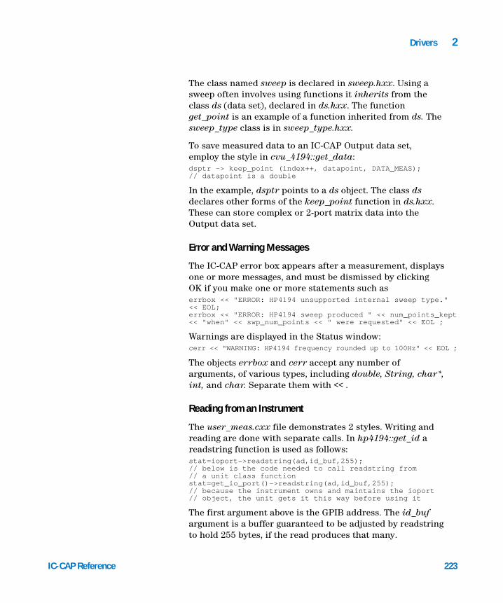
Drivers 2
IC-CAP Reference
The class named sweep is declared in sweep.hxx. Using a sweep often involves using functions it inherits from the class ds (data set), declared in ds.hxx. The function get_point is an example of a function inherited from ds. The sweep_type class is in sweep_type.hxx.
To save measured data to an IC-CAP Output data set, employ the style in cvu_4194::get_data:dsptr -> keep_point (index++, datapoint, DATA_MEAS); // datapoint is a double
In the example, dsptr points to a ds object. The class ds declares other forms of the keep_point function in ds.hxx. These can store complex or 2-port matrix data into the Output data set.
Error and Warning Messages
The IC-CAP error box appears after a measurement, displays one or more messages, and must be dismissed by clicking OK if you make one or more statements such aserrbox << "ERROR: HP4194 unsupported internal sweep type."<< EOL;errbox << "ERROR: HP4194 sweep produced " << num_points_kept<< "when" << swp_num_points << " were requested" << EOL ;
Warnings are displayed in the Status window:cerr << "WARNING: HP4194 frequency rounded up to 100Hz" << EOL ;
The objects errbox and cerr accept any number of arguments, of various types, including double, String, char*, int, and char. Separate them with << .
Reading from an Instrument
The user_meas.cxx file demonstrates 2 styles. Writing and reading are done with separate calls. In hp4194::get_id a readstring function is used as follows: stat=ioport->readstring(ad,id_buf,255);// below is the code needed to call readstring from// a unit class functionstat=get_io_port()->readstring(ad,id_buf,255);// because the instrument owns and maintains the ioport // object, the unit gets it this way before using it
The first argument above is the GPIB address. The id_buf argument is a buffer guaranteed to be adjusted by readstring to hold 255 bytes, if the read produces that many.
223

224
2 Drivers
A function is also provided to write a query and then read an answer: if ( ioport->write_n_read(addr,"MKRB?", urbuf, 80) == -1 )
The first argument above is the GPIB address. The second argument is a char* to be written. The third argument is a buffer guaranteed to be adjusted by readstring to hold 80 bytes, if the read produces that many.
The above functions are 2 of many available for an hpib_io_port. Complete declarations of its functions are in io_port.hxx.
Serial Poll of an Instrument
The following functions are 2 of many available for an hpib_io_port. Complete declarations of its functions are in io_port.hxx.
Serial polling is done as follows: int status_byte = ioport->spoll(addr); // this example not from user_meas.cxx int status_byte = get_io_port()->spoll(addr); // call from a unit function
To wait for a particular serial poll bit: // from cvu_4194::zero_supply:hpib_io_port *ioport = get_ioport();// bit-weight 1 below is to await ’measurement complete bit’if ( ioport -> poll_wait(addr, 1, 0, 10.0) == -1 )
The arguments are: GPIB address, bit-weight to wait for, a flag reserved for future use, and maximum time that poll_wait should try (10 seconds).
String Handling
C++ offers a substantial improvement over C for handling String type data. In the file String.h a number of String functions are declared. The following code demonstrates several.
IC-CAP Reference

Drivers 2
String str_hello = "hello" ; // declare and initialize a string String str_world ; // just declarestr_world = "world" ; // assignmentString hello_world = str_hello + " " + str_world ;// concatenationerrbox << hello_world + "0 ; // writing to errboxif ( "hello world" == hello_world ) // test for equalityString instr_cmd = "*RST" ; // initialize for next statement: if ioport->writestring(addr,instr_cmd) == -1 ) // String to instrument
IC-CAP Reference
In the final example, a char* is expected by writestring, and C++ automatically extracts it from the String. Do not pass a String to printf or scanf. The declarations of these functions in /usr/include/stdio.h use the ellipsis notation (...), so C++ does not know that a char* should be passed to them.
Time Delay
An example of a time delay is: delay ( 10E-3 ) ; // 10 millisecond delay
User Input with a Dialog Box
A number of functions for this purpose are declared in dialog.hxx. Examples to get data from dialog boxes are:
// These use the versions of get_double and get_String that// each take 3 arguments.double double_result ;String String_result ;int ok_or_cancel ; // 0 => OK pressed by user, and -1 => CANCELok_or_cancel = get_double ("Give a double:",default_dbl_val,&double_result);ok_or_cancel = get_String ("Give a string:",default_string,&String_result);
Writing to an Instrument
An example of writing to an instrument is:if ( ioport->writestring(addr,"TRIG") == -1 ) // cvu_4194::zero_supply
The arguments are the GPIB address and a char* string to send. You can also write a query and read a response with 1 call, write_n_read, discussed in Reading from an Instrument. Writestring and write_n_read are 2 of many functions available for an hpib_io_port. Complete declarations of its functions are in io_port.hxx.
225

226
2 Drivers
Syntax
This section provides help with reading the IC-CAP source code in user_meas.hxx, user_meas.cxx, and the various include files. Follow the example code in user_meas.hxx and user_meas.cxx when implementing a new driver.
NOTE For best results when using the vi editor to browse the source files, execute the command :set tabstop=3
The C++ language introduces several keywords to help understand OMI programming, for example, class, new, delete, and virtual. Terms that are peculiar to OMI programming, for example, Measurer, sweep type, sweep order, main sweep, internal sweep, user sweep, unit function, and instrument data, are used in this chapter and in the source files.
Function declarations in C++ use the improved function prototypes of ANSI/C. For example, int mult_by_2(int input);// style for forward declaration int y=2 ;int y = 2 ;int x = mult_by_2(y) ; // example of invocationint mult_by_2(int input)// style for implementation (SAME AS DECLARATION){
return 2*input ;}
This is an area of incompatibility with original (Kernighan and Ritchie) C. However, it is easier to read, and write, and is the emerging new standard. It also gives the compiler information with which function call argument lists can be checked, saving run-time aggravation.
Sometimes in class declarations you will see the function body present: const char *class_name() // this code from user_meas.hxx{ return “cvu_4194” ; }
IC-CAP Reference

Drivers 2
IC-CAP Reference
These cases are called inline functions. They behave like normal functions, but the C++ compiler emits code inline, without normal function call overhead. For short functions this reduces both execution time and code size.
New Symbols and Operators
This section defines new symbols and operators in C++.
// A pair of slashes introduces an end-of-line comment. ( /* and */ can still be used for C-style comments.)
& Appearing after a type name or class name, & usually indicates that an argument to a function is passed by reference. Although C can pass arguments by address, the C++ notion of reference arguments eliminates many error-prone uses of * (pointer de-reference) and & (address) operators used with pointer handling in C. In the following example, the called function increments the callers variable:// ’input’ passed by reference:void increment(int& input) {
input++ ; // need not use *input}int x=3;increment(x); // Need not pass &x// Now x is equal to 4
object. member_function( ) In C, the . operator is used to access data members in a struct object. In C++, . is also used to access (execute) function members.
ptr_to_object->member_function() In C, the -> operator is used to access data members in a struct object to which one holds a pointer. In C++, -> is also used to access (execute) function members of a class type object to which you hold a pointer.
227

2 Drivers
Class Hierarchy for User-Contributed Drivers
228
cvu_4194
user_unit
unit
inherits
inherits
The diagram in the following figure depicts the relationships of the classes that are of principle interest to a user creating a driver. The arrows without labels indicate pointers held in the objects.
At the top of the hierarchy are classes named unit, instr, and instr_options. All instrument drivers in IC-CAP consist of classes derived from these 3 classes. When Agilent Technologies adds a driver to IC-CAP, one new class is derived from instr, one or more new classes are derived from unit, and one new class is derived from instr_options. The process of deriving new classes from these base classes permits the new driver to efficiently reuse generic
Figure 6 Classes Involved in the HP 4194 Example of a User Driver
user_instr_options
hp4194_table
instr_options
hp4194
user_instr
instr
inherits inherits
inheritsinherits
IC-CAP Reference

Drivers 2
IC-CAP Reference
functionality present in the base classes, while also introducing new code where necessary to accommodate the specialized needs of the new instrument.
The division of a driver into unit, instr, and instr_options components helps modularity. Generally, the role of each of these parts is as follows:
• instr - manages operations associated with the whole instrument, such as self-test and initialization.
• instr_options - presents a user interface for and stores the values of options unique to each Setup in which an instrument is used. For example, the option Use User Sweep determines whether an instrument does or does not use its internal sweep capability during measurement in a particular Setup.
• unit - manages operations on a single SMU for example, in the case of a DC analyzer, or on a single oscilloscope input, in the case of a multi-channel digitizing oscilloscope like the 54120 series. Operations undertaken at this level include the application of DC and other signals to the DUT, as well as the acquisition of the measured data.
Intermediate in the hierarchy are 3 classes named user_unit, user_instr, and user_instr_options. These serve the following purposes:
• Hide any virtual functions of unit and instr that are unlikely to be necessary to override in new driver classes. This allows the critical function declarations to be concentrated in one location, with comments close at hand.
• Introduce new member functions provided for Instrument Options management or for convenience.
At the bottom of the hierarchy are examples of classes introduced by the Driver Generation Scripts. When a user adds a driver to IC-CAP, the Driver Generation Scripts add a class derived from user_instr, one or more classes derived from user_unit, and a class derived from user_instr_options. The class derived from user_instr_options, which is hp4194_table in the example driver, is completely declared
229

230
2 Drivers
and implemented when the user runs the mk_instr_ui script. In other words, a programmer using the Open Measurement Interface need not become involved with any coding that pertains to this user interface component of the driver. The programmer also does not need to provide declarations for any new classes needed for the driver, since these are completely written out when the driver generation scripts mk_unit, mk_instr, and mk_instr_ui are run. However, the programmer is required to fill-in the implementations of several functions that ultimately perform the work done by the driver.
IC-CAP Reference

Drivers 2
Order in Which User-Supplied Functions are Called
IC-CAP Reference
Table 60 through Table 63 illustrate the following 3 essential instrument operations:
• Rebuild (instrument list)
• Calibrate
• Measure
These tables are representative of a typical order of invocation. Some functions may be used more than once, particularly since Measure involves looping through different bias levels. The column Function Category indicates the location of further information about the function in “What Makes up an IC-CAP Driver” on page 209. Other valuable information is located in the comments for each function, provided in user_instr.hxx, user_unit.hxx, user_meas.hxx, and user_meas.cxx.
During RebuildDuring this operation, the Hardware Manager locates addresses that respond to a serial poll. At each such address, available drivers determine if they own the instrument, until 1 driver succeeds. They try in the order shown in the Instrument Library list. Note that unless find_instr() is successful, none of the ensuing functions are called.
The functions called during Rebuild (instrument list) are shown in the following table.
231
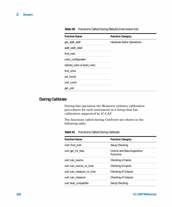
232
2 Drivers
Table 60 Functions Called During Rebuild (instrument list)
Function Name Function Category
get_addl_addr Hardware Editor Operations
addl_addr_label
find_instr
units_configurable
rebuild_units or build_units
find_units
set_found
unit_count
get_unit
During Calibrate
During this operation the Measurer initiates calibration procedures for each instrument in a Setup that has calibration supported by IC-CAP.
The functions called during Calibrate are shown in the following table.
Table 61 Functions Called During Calibrate
Function Name Function Category
instr::find_instr Setup Checking
unit::get_int_bias Control and Data Acquisition Functions
unit::can_source Checking of Inputs
unit::can_source_vs_time Checking of Inputs
unit::can_measure_vs_time Checking of Outputs
unit::can_measure Checking of Outputs
unit::bias_compatible Setup Checking
IC-CAP Reference

Drivers 2
IC-CAP Reference
unit::check_sweep Checking of Inputs
unit::check_sync Checking of Inputs
instr::cal_possible Calibration
instr::find_instr Setup Checking
instr::do_cal Calibration
Table 61 Functions Called During Calibrate (continued)
Function Name Function Category
During Measure
This operation undertakes a potentially complex series of operations on the instruments used by a Setup. The exact functions called vary, depending on whether calibration is available for particular instruments, and whether the main sweep instrument operates in an internally swept fashion, or in a stepped/spot-mode fashion (the case when the instrument option Use User Sweep is set to Yes for the main sweep instrument).
The functions called during Measure are shown in the following table (user main sweep) and Table 63 (internal main sweep).
Table 62 Functions Called During Measure (with User Main Sweep)
Function Name Function Category Notes
instr::find_instr Setup Checking
instr::find_units Hardware Editor Operations
instr::set_found Hardware Editor Operations
unit::get_int_bias Control and Data Acquisition Functions
unit::can_source Checking of Inputs
unit::can_source_vs_time Checking of Inputs
233

234
2 Drivers
unit::can_measure_vs_time Checking of Outputs
unit::can_measure Checking of Outputs
unit::bias_compatible Setup Checking
instr::reset_instr_info Initialization
unit::check_sweep Checking of Inputs
unit::check_sync Checking of Inputs
instr::reset_outptrs Initialization
unit::check_out Checking of Outputs
unit::can_do_second_sweep Control and Data Acquisition Functions
instr::cal_possible Calibration
instr::recall_n_chk_calib Calibration
instr::init_instr Initialization
instr::zero_supplies Initialization
BEGIN BIAS LOOP Loop to END BIAS LOOP
unit::set_bias Control and Data Acquisition
unit::enable_output Initialization
unit::set_scalar Control and Data Acquisition
BEGIN USER MAIN SWEEP LOOP
Loop to END MAIN SWEEP
unit::wait_hold_time Control and Data Acquisition
unit::set_bias Control and Data Acquisition
Table 62 Functions Called During Measure (with User Main Sweep)
Function Name Function Category Notes
IC-CAP Reference

Drivers 2
IC-CAP Reference
unit::set_sync Control and Data Acquisition
unit::wait_delay_time Control and Data Acquisition
unit::get_data Control and Data Acquisition
unit::get_scalar_data Control and Data Acquisition
END MAIN SWEEP LOOP
END BIAS LOOP
instr::zero_supplies Initialization
unit::fill_outds Control and Data Acquisition
Table 63 Functions Called During Measure (with Internal Main Sweep)
Function Name Function Category Notes
instr::find_instr Setup Checking
instr::find_units Hardware Editor Operations
instr::set_found Hardware Editor Operations
unit::get_int_bias Control and Data Acquisition Functions
unit::can_source Checking of Inputs
unit::can_source_vs_time Checking of Inputs
unit::can_measure_vs_time Checking of Outputs
unit::can_measure Checking of Outputs
unit::bias_compatible Setup Checking
Table 62 Functions Called During Measure (with User Main Sweep)
Function Name Function Category Notes
235

236
2 Drivers
instr::reset_instr_info Initialization
unit::check_sweep Checking of Inputs
unit::check_sync Checking of Inputs
instr::reset_outptrs Initialization
unit::check_out Checking of Outputs
unit::can_do_second_sweep Control and Data Acquisition Functions
instr::cal_possible Calibration
instr::recall_n_chk_calib Calibration
instr::init_instr Initialization
instr::zero_supplies Initialization
BEGIN BIAS LOOP Loop through ENDBIAS LOOP below
unit::set_bias Control and Data Acquisition
unit::enable_output Initialization
unit::set_scalar Control and Data Acquisition
unit::enable_sync Control and Data Acquisition
unit::set_2_internal_sweeps Initialization
unit::set_internal_sweep Initialization
unit::set_bias Control and Data Acquisition
unit::set_sync Control and Data Acquisition
unit::trigger Control and Data Acquisition
Table 63 Functions Called During Measure (with Internal Main Sweep)
Function Name Function Category Notes
IC-CAP Reference

Drivers 2
IC-CAP Reference
unit::wait_data_ready Control and Data Acquisition
unit::get_data Control and Data Acquisition
unit::get_scalar_data Control and Data Acquisition
END BIAS LOOP
instr::zero_supplies Initialization
unit::fill_outds Control and Data Acquisition
Table 63 Functions Called During Measure (with Internal Main Sweep)
Function Name Function Category Notes
237

2 Drivers
Handling Signals and Exceptions
238
A variety of conditions may result in termination of a measurement. Among the most common exceptions for a driver is an I/O timeout. Timeouts usually occur when one or more of the following conditions is present:
• Instruments are turned off
• Cabling is incorrect
• The driver software makes errors with respect to instrument protocol or the time required by the instrument’s operations
There are numerous examples in the hp4194 and cvu_4194 functions code that demonstrate setting the timeout before making different queries to the instrument. A timeout is usually detected as a value of -1, returned from the spoll, readstring, or writestring functions of the hpib_io_port used by the driver software.
In addition to instrument I/O problems, either of the following signals may be generated:
• SIGFPE This signal occurs when the code executes an operation like a divide by zero. By default, there is no provision in IC-CAP for trapping this signal.
NOTE If this signal occurs during Measure, the default handling of SIGFPE terminates the measurement; if it occurs during the execution of a transform, the function or macro will continue to execute and upon completion, an error message is displayed indicating a floating point error occurred.
• SIGINT This signal is generated when you issue the Interrupt command. By default, there is no provision in IC-CAP for trapping this signal. The measurement is terminated immediately. Note: For complex operations, it may take several minutes before control is returned.
IC-CAP Reference

Drivers 2
IC-CAP Reference
If your application requires special error recovery for these signals, it is possible to trap them. For details, refer to “Handling Signals and Exceptions" in the User’s Guide.
NOTE Do not alter the handling of SIGUSR1 and SIGUSR2; both signals are used internally by IC-CAP for error trap and recovery purposes.
239

2 Drivers
240 IC-CAP Reference

Agilent 85190A IC-CAP 2008Reference
3SPICE Simulators
SPICE Simulation Example 244
Piped and Non-Piped Simulations 246
Output Data Formats 252
SPICE Parameter Sweeps 254
Circuit Model Descriptions 256
Circuit Description Syntax 263
SPICE Simulator Differences 267
Using the PRECISE Simulator with IC-CAP 269
Using the PSPICE Simulator with IC-CAP 272
This chapter describes the details of using the SPICE simulators with IC-CAP. For general information on IC-CAP simulation, refer to Chapter 6, “Simulating,” in the User’s Guide.
NOTE The Solaris OS must include the cpp utility, which IC-CAP uses to manage output from SPICE simulators. See “System Requirements" in the Installation and Configuration Guide for more details.
IC-CAP can interface with the following SPICE simulators. They are provided as a courtesy to IC-CAP users (though not supported by Agilent Technologies), and you must purchase a license to use them.
• SPICE2 The SPICE2G.6 simulator developed at U.C. Berkeley.
• SPICE3 The SPICE3E2 simulator developed at U.C. Berkeley.
241Agilent Technologies

242
3 SPICE Simulators
• HPSPICE The Agilent Technologies implementation of SPICE2. Although there are some differences between this version and the SPICE2G.6 version from U.C. Berkeley, these 2 simulators are compatible. For more information refer to “SPICE Simulator Differences” on page 267. The version of HPSPICE provided with IC-CAP can be run only from within the IC-CAP program—it cannot be run stand-alone.
NOTE The HSPICE simulator, developed by Cadence, uses input deck syntax similar to that of the SPICE-type simulators; thus, it is referred to as a SPICE-type simulator in this manual. IC-CAP currently supports only the features of HSPICE also available in the U.C. Berkeley SPICE simulators.
The SPICE simulators support the following analysis types:
• DC
• AC
• Transient
• Noise
• Capacitance Voltage (CV)
• 2-Port (S,H,Y,Z,K,A parameter)
• Time-Domain Reflectometry (TDR)
NOTE The latter 3 simulation types are not directly available in the SPICE simulators; IC-CAP builds the additional circuitry required in the simulator input files to perform the simulation.
IC-CAP supports the features of ELDO that are also available in the UCB SPICE simulators but also provides limited support for models written in either ELDO-FAS or HDL-A. ELDO is an analog simulator developed by Mentor Graphics Corp. ELDO input deck syntax is compatible with that of the SPICE type simulators; therefore, in ELDO is categorized as a SPICE-type simulator this manual.
IC-CAP Reference

SPICE Simulators 3
IC-CAP Reference
The IC-CAP version of SPICE3 supports the following models:
The following additional SPICE-like simulators are also discussed in this chapter:
• PRECISE
• PSPICE
Model Group Supported Models Model Files
MOSFET Level 1, Level 2, Level 3 nmos/pmos2nmos3/pmos3
BSIM3, BSIM4 BSIM3_DC_CV_MeasureBSIM3_DC_CV_ExtractBSIM3_RF_MeasureBSIM3_RF_ExtractBSIM3_AC_Noise_TutorialBSIM3_CV_TutorialBSIM3_DC_TutorialBSIM3_Temp_TutorialBSIM3_DC_CV_FinetuneBSIM4_DC_CV_MeasureBSIM4_DC_CV_ExtractBSIM4_RF_MeasureBSIM4_RF_ExtractBSIM4_DC_CV_TutorialBSIM4_DC_CV_Finetune
MOS Model 9 mm9mm9_demo
BJT Gummel Poon bjt_npn/bjt_pnpbjt_nhfbjt_ncehfbjt_ftmnsnpnsabernpn
GaAs Statz UCBGaasUGaashf
Diode PN Diode pn_diode
Philips JUNCAP juncap
243

3 SPICE Simulators
SPICE Simulation Example
244
The circuit description is predefined for all IC-CAP configuration files. Enter this description if a new model is being defined; edit the description to fit specific needs. The syntax is identical to the syntax used for describing circuits in a typical SPICE simulation deck.
This simulation example will use the IC-CAP supplied Model bjt_npn.mdl.
1 Select the simulator by choosing Tools > Options > Select Simulator > spice2. Choose OK.
2 Choose File > Open > bjt_npn.mdl. Choose OK.
3 View the circuit description by clicking the Circuit tab.
The circuit description is shown in Figure 7. This deck describes the circuit (in this case, a single device) to be used in the simulation.
4 To view input and output for the fearly setup, click the DUTs-Setups tab and select fearly.
The Measure/Simulate folder appears with the inputs vb, vc, ve, and vs, and the output ic. The vc input specifies a voltage source at node C that sweeps linearly from 0 to 5V in 21 steps. The ic output specifies that current at node C be monitored.
In the Plots folder, icvsvc is specified so that the results of the simulation can be viewed graphically.
5 To simulate, click the Simulate button in the Measure/Simulate folder. The Status line displays Simulate in progress.
When the simulation is complete, the Status line displays IC-CAP Ready.
6 To view the results of the simulation, display the Plots folder and click Display Plot. The plot displays measured data represented by solid lines and simulated data represented by dashed lines.
IC-CAP Reference

SPICE Simulators 3
NOTE For syntax examples of running a remote simulation, refer to “Remote Simulation Examples" in the User’s Guide.
IC-CAP Reference
Q1 1 = C 2 = B 3 = E 4 = S NPN AREA = 1.0.MODEL NPN NPN+ IS = 36.76e-18 + BF = 336.1 + NF = 1.003 + VAF = 35.25+ IKF = 22.07m + ISE = 1.882f + NE = 1.932 + BR = 4.103+ NR = 1.005 + VAR = 1.651 + IKR = 147.3u + ISC = 15.69f+ NC = 1.857 + RB = 522.0 + IRB = 61.43u + RBM = 1.000m+ RE = 8.435 + RC = 57.05 + XTB = 1.700 + EG = 1.110+ XTI = 3.000 + CJE = 44.06f + VJE = 871.7m + MJE = 429.9m+ TF = 10.49p + TR = 1.700m + XTF = 247.4 + VTF = 1.622+ ITF = 140.6m + PTF = 218.8 + CJC = 68.94f + VJC = 603.8m+ MJC = 290.6m + XCJC = 300.0m + TR = 1.700n + CJS = 111.9f+ VJS = 465.0m + MJS = 241.9m + FC = 500.0m
Figure 7 Circuit Description Deck for an NPN Bipolar Transistor
245
3 SPICE Simulators
Piped and Non-Piped Simulations
246
The following sections describe the differences in piped and non-piped simulations for the various SPICE simulators. Each section also describes the argument syntax required to invoke each of the template simulators. This information is needed when writing the user translation module, since these are the arguments supplied by IC-CAP when it calls the translation module. For information on the translation module and adding a simulator, refer to the section “Adding a Simulator" in the User’s Guide.
Piped and Non-Piped SPICE Simulations
A non-piped simulation receives the input deck information from a file, performs the simulation and sends the binary output data and resulting text output to other files. The simulator process is restarted for every simulation.
A piped simulation receives the input deck information from a pipe connected to standard input, performs the simulation and sends the output data to a pipe connected to standard output. The simulator process will remain on until another simulator is selected. Setting the RETAIN_SIMU variable to TRUE overrides this behavior and allows multiple simulators to remain running. This uses additional memory but increases speed when frequently switching between simulators. In all cases, a piped simulator process will be turned off when the Simulation Debugger is turned on.
The text output from a simulation usually contains an explanation of any errors which may have been encountered during the simulation. Piped simulations do not save any text output from the simulation. If an error occurs during a piped simulation, IC-CAP issues a message in an error box stating that an error has occurred and recommending that the simulation be repeated with the Simulation Debugger turned on. IC-CAP performs non-piped simulations when the Simulation Debugger is ON.
IC-CAP Reference
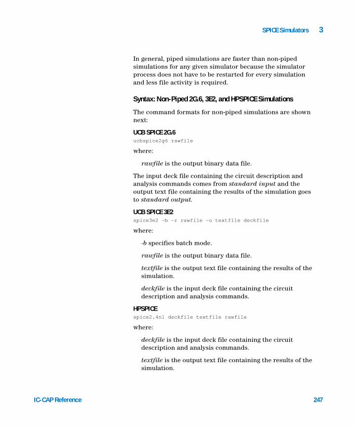
SPICE Simulators 3
IC-CAP Reference
In general, piped simulations are faster than non-piped simulations for any given simulator because the simulator process does not have to be restarted for every simulation and less file activity is required.
Syntax: Non-Piped 2G.6, 3E2, and HPSPICE Simulations
The command formats for non-piped simulations are shown next:
UCB SPICE 2G.6 ucbspice2g6 rawfile
where:
rawfile is the output binary data file.
The input deck file containing the circuit description and analysis commands comes from standard input and the output text file containing the results of the simulation goes to standard output.
UCB SPICE 3E2 spice3e2 -b -r rawfile -o textfile deckfile
where:
-b specifies batch mode.
rawfile is the output binary data file.
textfile is the output text file containing the results of the simulation.
deckfile is the input deck file containing the circuit description and analysis commands.
HPSPICE spice2.4n1 deckfile textfile rawfile
where:
deckfile is the input deck file containing the circuit description and analysis commands.
textfile is the output text file containing the results of the simulation.
247

248
3 SPICE Simulators
rawfile is the output binary data file.
Syntax: Piped 2G.6, 3E2, and HPSPICE Simulations
The command formats for piped simulations are shown next:
UCB SPICE 2G.6 ucbspice2g6 -
where:
The "-" denotes that the binary data output is going to the standard output pipe. The input deck information comes from the standard input pipe and the output text is sent to the file /dev/null.
UCB SPICE 3E2 spice3e2 -s
where:
The -s option specifies that the input deck information is coming from standard input and the binary data output is going to standard output.
HPSPICE spice2.4n1 - /dev/null -
where:
The first "-" denotes that the input deck information is coming from the standard input pipe.
The output text is sent to the file /dev/null.
The last "-" denotes that the binary data output is going to the standard output pipe.
IC-CAP Reference
SPICE Simulators 3
Non-Piped HSPICE Simulations
NOTE Starting with the IC-CAP 2008 release, the CAN_PIPE token for HSPICE in usersimulators is supported. This token can now be used on local HSPICE and local Solaris HSPICE simulations with HSPICE-2007.03.SP1. It is not a true piped mode (netlists and raw files are still written to disk), but provides substantial performance improvement by using an interactive mode that avoids restarting HSPICE for every simulation. Beginning in HSPICE 2008.03-SP1, HSPICE license will time out in 1800 seconds for CAN_PIPE mode. You can customize the license timeout by setting variable HSPICE_LICENSE_TIMEOUT (unit by second).
IC-CAP Reference
Non-piped HSPICE simulations are identical to non-piped SPICE simulations. This type of simulation is performed when the Simulation Debugger is set to ON. If CANNOT_PIPE is specified for HSPICE, even when the Simulation Debugger is OFF, it still performs a non-piped simulation. This means that HSPICE must be restarted for every simulation. Because of this, there is no noticeable difference in simulation speed when the Simulation Debugger is set to ON or OFF.
Syntax: Piped HSPICE Simulations
The command format for an HSPICE piped simulation is as follows:
hspice -I
load deckname and run commands are then passed to the running HSPICE process.
Syntax: Non-Piped HSPICE Simulations
The command format for an HSPICE non-piped simulation is as follows:
hspice -i deckfile -o logfile
where
deckfile is the input deck file containing the circuit description and analysis commands.
249

250
3 SPICE Simulators
logfile is the listing of information about the simulation generated by HSPICE. If the simulation debugger is open, this file will be displayed in the Output Text portion of the simulation debugger.
The output binary data file is written to a file named deckfile.suffix where suffix depends on the type of analysis being performed. Refer to the HSPICE User's Manual for more information.
Syntax: Client/Server mode HSPICE Simulations
On Windows, provides a method of invoking a standing server process to access HSPICE licenses. If this was launched via the hspui program, IC-CAP can simulate faster by launching HSPICE with the followin syntax:
hspice -C deckfile -o logfile
where
deckfile is the input deck file containing the circuit description and analysis commands.
logfile is the listing of information about the simulation generated by HSPICE. If the simulation debugger is open, this file will be displayed in the Output Text portion of the simulation debugger.
However, if the server has not been started, the simulation still occurs but at a slower speed.
To configure IC-CAP to send the -C instead of -i, specify the template name hspice-C as the second field in your usersimulators line example:hspiceC hspice-C c:\synopsys\Z-2007.09\bin\hspice.exe "" CANNOT_PIPE
Non-Piped ELDO Simulations
Non-piped ELDO simulations are identical to non-piped SPICE simulations. This type of simulation is performed when the Simulation Debugger is set to ON. ELDO is not capable of performing a piped simulation, so even when the Simulation Debugger is OFF, it still performs a non-piped simulation. This
IC-CAP Reference

SPICE Simulators 3
IC-CAP Reference
means that ELDO must be restarted for every simulation. Because of this, a there is no noticeable difference in simulation speed when the Simulation Debugger is set to ON or OFF.
Syntax: Non-Piped ELDO Simulations
The command format for an ELDO non-piped simulation is as follows:eldo deckfile
where
deckfile is the input deck file containing the circuit description and analysis commands. The name of this deckfile is in the form <circuit_name>.cir.
The output binary data file is written to a file named <circuit_name>.spi3. This output binary data format is similar to the output binary format of the UCB SPICE3 simulator and is generated when you specify the option .option spi3bin
Refer to the ELDO User’s Manual for more information.
The output text file, is sent to the file named <circuit_name>.chi This file is displayed in the Output table of the Simulation Debugger if it is on.
251

3 SPICE Simulators
Output Data Formats
252
The example in the following figure shows the output data format of the spice2 template simulator supported in IC-CAP.
Record 1: Title card (80 bytes), date (8 bytes), time (8 bytes) TOTAL-96 BYTESRecord 2: Number of output variables (including "sweep" variable) (2 bytes)Record 3: Integer ’4’ (2 bytes)Record 4: Names of each output variable (8 bytes each)Record 5: Type of each output (2 bytes each) 0 = no type 1 = time 2 = frequency 3 = voltage 4 = current 5 = output noise 6 = input noise 7 = HD2 8 = HD3 9 = DIM2 10 = SIM2 11 = DIM3 Outputs 7 through 11 are distortion outputs.Record 6: The location of each variable within each sweep point. (2-bytes each) (Normally just 1,2,3,4,...but needed if outputs are mixed up)Record 6a: 24 characters that are the plot sub-title if Record 3 is a ’4’.Record 7: Outputs at first sweep pointRecord 8: Outputs at second sweep pointRecord 9: . . .last recordAll real data are 8-byte quantities.All complex data are single precision reals, that is 4-byte quantities. (4-byte quantity for the real part, 4-byte quantity for the imaginary part)EOF A special "end-of-file" indicator: 9.87654321D+27 for real data (9.876E+0,5.432E+0) for complex dataEOI A 4 byte integer zero indicates the end of all raw data
Figure 8 Output File Format Used For spice2
The binary format output by the spice3 template simulator is shown in the following figure.
IC-CAP Reference

SPICE Simulators 3
Title Card (Newline (\n) terminated string)Date and Time (Newline (\n) terminated string)Plot Title (Newline (\n) terminated string)Flags (Newline (\n) terminated string)Number of Variables (No. Variables: [an integer])Number of Points (No. Points: [an integer])Version (Newline (\n) terminated string)Variables List (Variables:
[tab] (index) [tab] (name) [tab] (type).
. . { repeated num_var times } where: index = variable index [integer] name = variable name [string] type = variable type [string (that is, "current" or "voltage")] num_var = number of variablesBinary: ( Newline (\n) terminated string indicating the start of the binary data )Each data point is listed in the order listed in the variables list.Each real data point is represented by 8 bytes.Each complex data point consists of the real part and the imaginary part of 8 bytes each.There are no separators between data points.
IC-CAP Reference
Figure 9 Output File Format Used For spice3
253

3 SPICE Simulators
SPICE Parameter Sweeps
NOTE Parameter sweeps should always be the outer most sweep.
LSYNC sweeps should have master sweeps that are also parameter sweeps.
254
For SPICE-type simulators, specifying parameter sweeps for devices and circuits requires an input added to the setup (in this example, nmos2/short/idvd) with Mode P.
Figure 10 SPICE Parameter Sweep Setup Example
IC-CAP performs a simulation for each value of the parameter sweep. The following figure shows the resulting plot.
IC-CAP Reference
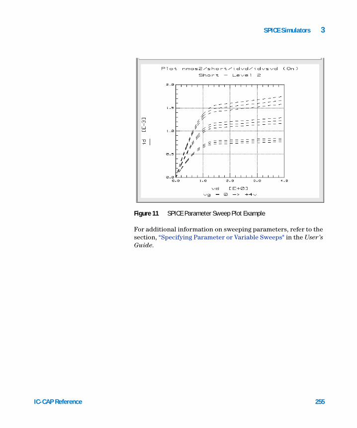
SPICE Simulators 3
IC-CAP Reference
Figure 11 SPICE Parameter Sweep Plot ExampleFor additional information on sweeping parameters, refer to the section, “Specifying Parameter or Variable Sweeps" in the User’s Guide.
255

3 SPICE Simulators
Circuit Model Descriptions
256
The circuit description for the HSPICE and ELDO simulators is similar to the UCB SPICE simulator circuit description. The details in the following sections also apply to HSPICE and ELDO.
Specifying Simulator Options
For information on available options and their syntax, refer to the User’s Manual for that simulator. Simulator options are specified in the first line of the circuit definition using the following syntax: .OPTIONS OPT1 = OPTVAL1 OPT2 = OPTVAL2 ... OPTN = OPTVALN
where
OPTs denote the option keywords used by the simulator
OPTVALs are the corresponding option values. Some options do not require a value; this field may or may not be specified, depending on the option.
A space is the only delimiter required between options.
The nominal and operating temperatures, TNOM and TEMP, are commonly used options; they can also be specified by entering a value (in °C) for the global variables TNOM and TEMP. To do this, enter the variable and its value in the System Variables table in the Utilities application.
• TNOM is the temperature at which the model parameters are extracted; TEMP is the temperature at which the simulation is performed. When performing an optimization to extract model parameters, TEMP and TNOM should be set to the same value so that simulations during optimization are performed at TNOM. TNOM must be defined to guarantee consistency between simulation and extraction.
IC-CAP Reference

SPICE Simulators 3
IC-CAP Reference
• In general, TNOM and TEMP can be in any variable table, allowing different Models, DUTs or Setups to use different nominal and operating temperatures. IC-CAP checks for these global variables before running a simulation. If the variable is not found, the value of the option set in the .OPTIONS statement in the Circuit Editor is used when it exists. Otherwise, the circuit is analyzed using the simulator’s default values.
IC-CAP automatically adds the option POST=1 to the options list when the selected simulator is hspice. Specifying this option causes hspice to return the binary raw data file, which IC-CAP requires for reading back the simulated data. This option is not necessary when performing a Manual Simulation from the Simulation Debugger command menu because the data is not read back into IC-CAP.
Describing the Device Model
A device model is used to characterize a single SPICE element of any type. This description requires 2 parts:
• An element statement that calls a defined model
• A .MODEL definition, which is identical to a .MODEL card in SPICE
The general form of the element statement that calls the device model is:DNAME NNUM1 = NNAME1 NNUM2 = NNAME2 ...NNUMN = NNAMEN MNAME+ DPAR1 = DVAL1 DPAR2 = DVAL2 ...DPARN = DVALN
where
DNAME is the device name with the first letter being a simulator defined key letter denoting the type of model being specified.
NNUM denotes the node number connections.
NNAME denotes node names corresponding to the node numbers.
DPAR is a predefined DUT parameter name.
257

258
3 SPICE Simulators
DVAL is the specified DUT parameter value. Refer to the SPICE Reference manual for DUT parameter names available for each model.
MNAME is the model name being referenced. This is the same MNAME specified in the .MODEL definition described below
A .MODEL definition specifies the parameters of a device model that describe a particular element. When a parameter is not specified, the default value in the model is used. The general form of the .MODEL definition is: .MODEL MNAME TYPE PNAME1=PVAL1 PNAME2=PVAL2 ...PNAMEN=PVALN
where
MNAME is the model name. Regardless of the model name entered in the MNAME field of the .MODEL definition statement, IC-CAP substitutes the name of the Model as it is called in the Model List when the simulator input deck is built.
TYPE is a valid SPICE component type
PNAME is a parameter name for the particular model type
PVAL is the parameter value
As in SPICE, a plus sign ( + ) that appears as the first character of a line denotes a continuation of the previous line. This continuation character is often used for easier readability when specifying the .MODEL card.
NOTE When using the SPECTRE simulator with either the OSI, SPECTRE442, or SPECTRE443 interfaces (see “SPECTRE Interfaces” on page 276), the LEVEL parameter for a MOS .MODEL card may not translate properly. IC-CAP outputs the value as a real number in the netlist, but SPECTRE requires an integer. To work around this issue, use the model type BSIM3 instead of MOS and omit the LEVEL parameter. Alternatively, enclose the LEVEL parameter with parentheses, for example, LEVEL = (11). By doing the later, IC-CAP does not flag it as a model parameter and leaves the expression alone when passing the netlist to SPECTRE.
IC-CAP Reference
SPICE Simulators 3
Describing Subcircuits
IC-CAP Reference
A subcircuit model is used to describe a circuit that contains more than 1 element.
The syntax is similar to the syntax in SPICE. The subcircuit description must begin with a .SUBCKT and end with a .ENDS declaration. Statements between these 2 declarations describe the subcircuit components.
The general form of the first line of a subcircuit definition is:.SUBCKT SUBNAME NNUM1 = NNAME1 NNUM2 = NNAME2 ...NNUMN =NNAMEN + (PAR1=PARVAL1 PAR2=PARVAL2 ...PARN=PARVALN)
where
SUBNAME is the name you give to the subcircuit. Regardless of the subcircuit name entered in the SUBNAME field of the .SUBCKT definition statement, IC-CAP substitutes the name of the Model being simulated when the simulator input deck is built.
NNUM are the numbers of the external nodes of the subcircuit. These external nodes are used to connect the subcircuit to another circuit. External nodes in the .SUBCKT declaration cannot be 0 (ground), but internal nodes can be connected to ground and any external node to ground in a surrounding circuit.
NNAME is a node name assigned to a node number. As in the device model description, IC-CAP allows the option of equating node numbers to node names. If you assign node names, use these names when specifying the Inputs and Outputs in the Setup.
PAR1 ... PARN are subcircuit parameters that can be passed through subcircuit calls. These parameters are added to the DUT parameter table in IC-CAP.
PARVAL1 ... PARVALN are the corresponding parameter values. These subcircuit parameters become DUT parameters and can be modified in the DUT Parameter Editor.
(While the syntax shown here is correct, passed parameters are ignored by IC-CAP.)
259

260
3 SPICE Simulators
The body of the subcircuit model description contains the components of the subcircuit using element and .MODEL statements.
Assigning Node Names
IC-CAP allows the option of equating node numbers to node names in circuit descriptions because it is typically easier to refer to a node by a meaningful name rather than a number. If node numbers only are specified, these node numbers must be used when specifying inputs and outputs. Node identities can also be specified with the format %<name>. For example:Q1 1=C 2=B 3=E 4=S NPN or Q1 %C %B %E %S NPN
Although HSPICE and ELDO allow alphanumeric characters for node names, node numbers must still be associated with node names because IC-CAP parses HSPICE as a SPICE-type simulator.
When using this format, all node names within the circuit or device must be referenced using the %[nodename] syntax.
Test Circuits and Hierarchical Simulation
When characterizing a circuit, it is often necessary to add circuitry around a circuit or device to model the actual measurement Setup. IC-CAP provides a Test Circuit Editor to allow modeling of this additional bias circuitry. Select the DUT from the DUT/Setup panel. Click the Test Circuit tab and enter the test circuit description in the same manner you would enter a Circuit Description. The test circuit definition should include a call to the device or subcircuit defined in the Circuit Editor, as well as the additional circuitry needed to model the external parasitics of the measurement Setup.
NOTE When you define a test circuit, the DUT parameter table contains the values specified in the test circuit specification. Regardless of the subcircuit name entered in the SUBNAME field of the .SUBCKT declaration, IC-CAP uses the name of the DUT being simulated when the simulator input deck is built.
IC-CAP Reference

SPICE Simulators 3
IC-CAP Reference
Subcircuit and device model specifications can be called from inside another Model. This enables you to perform hierarchical simulations to study a circuit at different levels.
When making reference to another model, the model name must be used as it appears in the IC-CAP Model List. For example, assume you have defined 3 Models, model1, model2, and model3. model1 has a circuit model description that is a device definition. The circuit model description for model2 is a subcircuit definition at the gate level that includes a call to model1 in a device call statement. And, the circuit model description for model3 is a subcircuit definition that includes a call to model2 in a subcircuit call statement. When you simulate a Setup in model3, IC-CAP traverses the Model hierarchy and uses the circuit model description defined in model3, which includes calls to model1 and model2. The syntax for calling a device model is identical to that described in the Device Model Description section.
The general form of the device call is: DNAME NNUM1 = NNAME1 NNUM2 = NNAME2 ...NNUMN = NNAMEN MNAME+ DPAR1 = DVAL1 DPAR2 = DVAL2 ...DPARN = DVALN
Calling a subcircuit specification allows you to insert an entire subcircuit into a circuit as if it were a single component. The call requires a syntax identical to that used in SPICE. The general form of the subcircuit call is: XNAME NNUM1 NNUM2 ...NNUMN SUBNAME (PARVAL1 PARVAL2 ... PARVALN)
where
XNAME is the name of the subcircuit call statement. The only requirement for this name is that it must start with the letter X.
NNUM are the node numbers of the calling circuit that connect to the external nodes of the subcircuit. The calling circuit node numbers need not be the same as the external nodes of the subcircuit. The nodes are connected in the order specified. Specify the same number of nodes declared in the subcircuit definition.
261

262
3 SPICE Simulators
SUBNAME is the name of the subcircuit, previously described by a .SUBCKT definition. This must have the name of the model as it appears in the Model List if it is in a different model.
PARVAL are subcircuit parameter values. The order in which they are listed in the subcircuit call statement must match the parameters list in the subcircuit definition.
(While the syntax shown here is correct, passed parameters are ignored by IC-CAP.)
NOTE When a test circuit is included in the Model, IC-CAP uses the test circuit description as the top level circuit definition. The node number connections defined in the test circuit description, not the circuit description, are used as the external nodes. Because of this, any node-number-to-node-name cross-referencing in the circuit description is not used. Only node names equated to node numbers in the test circuit description can be used when specifying Inputs and Outputs in the Setup Editor. When only node numbers are specified in the test circuit description, (that is, they are not equated to node names) these same node numbers must be used in the Input and Output node fields.
IC-CAP Reference

SPICE Simulators 3
Circuit Description Syntax
IC-CAP Reference
This section describes basic syntax rules for creating a circuit description.
SPICE Simulators
Start an input line with * to denote a comment in the circuit model description or in the input file of the simulation debugger. Although some simulators accept # and * , IC-CAP accepts * only. (# is recognized as a preprocessor directive when the simulator input deck is built. Adding a comment using # causes a simulation generated from a DUT or Setup to fail.)
The following table lists the SPICE element component specifications. For information on available options and their syntax, refer to the SPICE Reference manual.
Table 65 lists the semiconductor device specifications. For information on available options and their syntax, refer to the SPICE Reference manual.
Table 64 SPICE Element Component Specifications
Component General Form Example
Resistor RXXXXXXX N1 N2 VALUE <TC=TC1<TC2>>
R1 1 2 1000 TC=0.001,0.015
Capacitor CXXXXXXX N+ N- VALUE <IC=INCOND>
COSC 15 2 10U IC=3
Inductor LXXXXXXX N+ N- VALUE <IC=INCOND>
LSHUNT 3 29 10U IC=15.7m
Mutual Inductor KXXXXXXX LYYYYYYY LZZZZZZZ VALUE
K43 LAA LBB 0.999
Transmission Line
TXXXXXXX N1 N2 N3 N4 Z0=VALUE<TD=VALUE>+ <F=FREQ <NL=NRMLEN>> <IC=V1,I1,V2,I2>
T1 1 0 2 0 Z0=50 TD=10NS
263

264
3 SPICE Simulators
Linear Voltage- Controlled Current Source
GXXXXXXX N+ N- NC+ NC- VALUE G1 2 0 5 0 0.1M
Linear Voltage- Controlled Voltage Source
EXXXXXXX N+ N- NC+ NC- VALUE E1 2 3 14 1 2.0
Linear Current- Controlled Current Source
FXXXXXXX N+ N- VNAM VALUE F1 13 5 VSENS 5
Linear Current- Controlled Voltage Source
HXXXXXXX N+ N- VNAM VALUE HX 5 17 VZ 0.5K
Independent Voltage Source
VXXXXXXX N+ N- <<DC> DC/TRAN VALUE> + <AC <ACMAG <ACPHASE>>>
VIN 12 0 DC 6
Independent Current Source
IXXXXXXX N+ N- <<DC> DC/TRAN VALUE> + <AC <ACMAG <ACPHASE>>>+ SFFM(0 1 10K 5 1K)
ISRC 23 21 AC0.333 45.0
Table 65 SPICE Semiconductor Component Specifications
Component General Form Example
Junction Diode
DXXXXXXX N1 N2 MNAME+ <AREA><OFF><IC=VD>
DCLAMP 3 7 DMOD 3.0 IC=0.2
BJT QXXXXXXX NC NB NE <NS> MNAME+ <AREA> <OFF> <IC=VBE,VCE>
Q2A 11 26 4 20 MOD1
JFET JXXXXXXX ND NG NS MNAME+ <AREA> <OFF> <IC=VDS,VGS>
J1 7 2 3 JM1 OFF
Table 64 SPICE Element Component Specifications (continued)
Component General Form Example
IC-CAP Reference

SPICE Simulators 3
IC-CAP Reference
MOSFET MXXXXXXX ND NG NS NB MNAME+ <L=VAL><W=VAL><AD=VAL><AS=VAL>+<PD=VAL><PS=VAL><NRD=VAL><NRS=VAL>+ <OFF> <IC=VDS,VGS,VBS
M1 2 9 3 0 MOD1 L=10U W=5U
Table 65 SPICE Semiconductor Component Specifications (continued)
Component General Form Example
HSPICE Simulator
Basic HSPICE syntax rules are the same as SPICE-type simulators. Refer to the HSPICE User’s Manual for complete syntax and rules.
ELDO Simulator
NOTE Before performing HSPICE simulations, specify the HSPICE version name in the System Variable HSPICE_VERSION. If this variable is not specified, IC-CAP will assume the latest version of HSPICE is being used.
Basic ELDO syntax rules are the same as SPICE-type simulators. In addition to the SPICE-type syntax, FAS user-defined models can be defined and instantiated in the IC-CAP Circuit Editor. An FAS model is defined as:amodel name(pin1,pin2..).<model body> . endmodel
(smodel and fmodel are also accepted).
The above model is instantiated in a circuit as:yxx name [pin:] 1 2 ... [param: par1 = var1 ...] [model: ...]
In addition, the parser accepts the following ELDO constructs:.ADDLIB number pathname#com . . #endcom
265
266
3 SPICE Simulators
FIDEL models (oxx p1:typ p2:typ ... mod=modelname) and transfer functions (FNS, FNZ) are not currently supported by the IC-CAP parser. However, the #echo keyword can be used to insert these statements into a circuit in the IC-CAP Circuit Editor.
The #echo keyword is available in the IC-CAP Circuit Editor for all supported simulators. #echo can be used to pass a deck card or command directly through to the simulator without any parsing by IC-CAP. For example, the line#echo <something that the IC-CAP parser doesn't understand>
is sent to the simulator as<something that the IC-CAP parser doesn't understand>
The following analog model instantiation syntax is supported for HDL-A:
HDL-A user-defined models with the following syntax can also be instantiated in the IC-CAP Circuit Editor.yxx name(xx) [pin:] 1 2 ... [param: par1 = var1 ...]
andyxx name(xx) [pin:] 1 2 ... [generic: par1 = var1 ...]
NOTE Before performing ELDO simulations specify the ELDO version name in the System Variable ELDO_VERSION. If this variable is not specified, IC-CAP will use the version name specified in the environment variable eldover, if it exists. If neither ELDO_VERSION or eldover are specified, IC-CAP assumes that the latest version of ELDO is being used.
IC-CAP Reference

SPICE Simulators 3
SPICE Simulator Differences
IC-CAP Reference
Subtle differences in syntax, behavior, error handling and calculation of data between the simulators must be considered when creating a circuit description.
• SPICE2 simulations will fail if an underscore is used in the Model name. An error message will appear in the output text file generated by the Simulation Debugger:
0*ERROR*: MODEL TYPE IS MISSING
• SPICE2 simulations will fail if an underscore is used in a test circuit and DUT name because the simulation input deck uses the DUT name as a model name. An error message will appear in the output text file:
0*ERROR*: SUBCIRCUIT NODES MISSING
• When attempting a SPICE2 or SPICE3 simulation in the BJT model, if the ideal maximum forward beta parameter BF=0 or the transport saturation current parameter IS=0, the simulation will fail without an error message. (Other parameters may yield similar results when set to zero.)
• SPICE3 is the only simulator that supports the UCB GaAs model. Refer to “Simulators" in the Nonlinear Device Models, Volume 1 manual for details on the syntax required to simulate this model.
• HPSPICE is the only simulator that supports the Curtice GaAs model. Refer to “Simulators" in the Nonlinear Device Models, Volume 1 manual for details on the syntax required to simulate this model.
• When using HPSPICE to simulate a UC Berkeley MOSFET model, specify the ucb option in the .OPTIONS statement of the circuit description:
.OPTIONS ucb
267

268
3 SPICE Simulators
• When using SPICE3 with the Simulation Debugger to perform an IC-CAP simulation (as opposed to a manual simulation), an output text file with the following message results: print card ignored since rawfile was produced. To generate a more informative output text file, perform a manual simulation. The manual simulation results in an output text file that includes the requested output data values.
IC-CAP Reference

SPICE Simulators 3
Using the PRECISE Simulator with IC-CAP
IC-CAP Reference
PRECISE is a UCB SPICE-based simulator developed by Mentor Graphics Corp. Using IC-CAP’s Open Simulator Interface, a C-language Translation Module is provided that makes PRECISE simulation capability available in IC-CAP. This module and instructions for performing PRECISE simulations in IC-CAP are described here. For general information on the Open Simulator Interface, refer to the section “Adding a Simulator" in the User’s Guide.
The IC-CAP/PRECISE link uses UCB SPICE2G.6 as the template simulator. When performing a PRECISE simulation in IC-CAP, IC-CAP behaves as if it is performing a SPICE2 simulation. Therefore it generates an input deck in SPICE2 format, calls the simulator and reads back a binary raw data file in SPICE2 format. Through the Open Simulator Interface, the call to the simulator is actually calling the executable version of the C-language Translation Module, precise.c. This executable, called precise, translates the SPICE2 input deck to a PRECISE input format, calls PRECISE to perform the simulation, then translates the PRECISE format binary raw data file to SPICE2 format which is read by IC-CAP. The source code file precise.c is located in the $ICCAP_ROOT/src directory.
To set up PRECISE simulation capability in IC-CAP:
1 Add the precise simulator to the usersimulators file in the directory $ICCAP_ROOT/iccap/lib, as shown next: precise spice2 /<your path>/precise "<host_machine_name>"CANNOT_PIPE
2 The host_machine_name is the host computer for the PRECISE simulations. This name can be left blank ("") if PRECISE and IC-CAP are running on the same computer. Since PRECISE does not have the ability to perform piped simulations in IC-CAP, the CANNOT_PIPE flag must always be set, as shown in the above example.
269

3 SPICE Simulators
NOTE The IC-CAP/PRECISE interface is only supported for the HP 9000 Series 700 version of PRECISE. Therefore the host computer must be a Series 700 workstation.
270
3 Make the following changes to the precise.c program to customize it for your environment:
• In the main routine, specify the full pathname of the actual PRECISE simulator on your system.
• In the spice2_to_precise routine, specify the full pathname of the Mentor Graphics supplied program ppphp700.exe, which translates a SPICE2 input deck to the equivalent PRECISE input deck.
4 Compile the translation module using the following command: cc -o precise precise.c -lm
5 Move the executable file, precise to a permanent location such as $ICCAP_ROOT/bin The location must match the path specified in the usersimulators file.
6 In IC-CAP, set the SIMULATOR variable to precise or specify precise with the Select Simulator command on the IC-CAP Tools Menu.
The following files are generated in your home directory when running PRECISE simulations in IC-CAP:
• namefile - File that contains the name of the spice input deck file indeck.spi.
• indeck.spi - SPICE 2G.6 format input deck file that is the input to the input deck translator program ppphp700.exe provided by Mentor Graphics.
• indeck.ckt - PRECISE format circuit description deck output from the input deck translator program ppphp700.exe.
• indeck.use - PRECISE format analysis command deck output from the input deck translator program ppphp700.exe.
• xndeck.use - PRECISE format analysis command deck referenced by indeck.use. Also generated by the input deck translation.
IC-CAP Reference

SPICE Simulators 3
IC-CAP Reference
• rawout - PRECISE formatted binary raw data output file generated by a PRECISE simulation.
271

3 SPICE Simulators
Using the PSPICE Simulator with IC-CAP
272
PSPICE is a SPICE-based circuit simulator developed by MicroSim Corporation. PSPICE uses the same basic numeric algorithms as the UCB SPICE2 simulator but claims superior convergence and performance. Using IC-CAP’s Open Simulator Interface, a C-language Translation Module is provided that makes PSPICE simulation capability available in IC-CAP. This module and instructions for performing PSPICE simulations in IC-CAP are described here. For general information on the Open Simulator Interface, refer to the section “Adding a Simulator" in the User’s Guide.
The IC-CAP/PSPICE link uses UCB SPICE2 as the template simulator. When performing a PSPICE simulation in IC-CAP, IC-CAP behaves as if it is performing a SPICE2 simulation. Therefore it generates an input deck in SPICE2 format, calls the simulator and reads back a binary raw data file in SPICE2 format. Through the Open Simulator Interface, the call to the simulator is actually calling the executable version of the C-language Translation Module, pspice.c. This executable, called pspice, translates the SPICE2 input deck to a PSPICE input format, calls PSPICE to perform the simulation, then translates the PSPICE format binary raw data file to SPICE2 format which is read by IC-CAP. The source code file pspice.c is located in the $ICCAP_ROOT/src directory.
NOTE The IC-CAP/PSPICE translation module pspice.c has been updated in IC-CAP 5.0 to support the output binary data format of PSPICE 6.3. Only PSPICE versions with the identical output binary data format will work with this translation module. For older PSPICE versions, use the translation module pspice5_4.c, also supplied with this release.
To set up PSPICE simulation capability in IC-CAP:
1 Add the pspice simulator to the usersimulators file in the directory $ICCAP_ROOT/iccap/lib, as shown next.pspice spice2 /<your path>/pspice "<host_machine_name>"CANNOT_PIPE
IC-CAP Reference

SPICE Simulators 3
IC-CAP Reference
2 The host_machine_name is the host computer for the PSPICE simulations. This name can be left blank ("") if PSPICE and IC-CAP are running on the same computer. Since PSPICE does not have the ability to perform piped simulations in IC-CAP, the CANNOT_PIPE flag must always be set, as shown in the above example.
3 Make the following change to the pspice.c program to customize it for your environment:
• In the main routine, specify the full pathname of the actual PSPICE simulator on your system.
4 Compile the translation module using the following command: cc -o pspice pspice.c -lm
5 Move the executable file, pspice to a permanent location such as ICCAP_ROOT/bin. The location must match the path specified in the usersimulators file.
6 In IC-CAP, set the SIMULATOR variable to pspice or specify pspice with the Select Simulator command in the IC-CAP Tools Menu.
The following files are generated in your home directory when running PSPICE simulations in IC-CAP:
• psp.cir - PSPICE format circuit description deck file translated from the SPICE2 circuit description deck.
• psp.raw - PSPICE formatted binary raw data output file generated by a PSPICE simulation.
• psp.out - Output print file generated by a PSPICE simulation.
psp.raw and psp.out are automatically removed from your home directory after the simulation is completed in IC-CAP.
NOTE When using PSPICE, the LM_LICENSE_FILE environment variable must be set. This variable contains the directory path for the license file required by the PSPICE simulator. Refer to the PSPICE Reference Manual for detailed procedures on installing the PSPICE simulator.
273

3 SPICE Simulators
274 IC-CAP Reference

Agilent 85190A IC-CAP 2008Reference
4SPECTRE Simulator
SPECTRE Interfaces 276
Circuit Model Descriptions 278
Piped and Non-Piped SPECTRE Simulations 288
This chapter describes the details of using the SPECTRE simulator with IC-CAP. For general information on IC-CAP simulation, refer to Chapter 6, “Simulating,” in the User’s Guide.
275Agilent Technologies

4 SPECTRE Simulator
SPECTRE Interfaces
276
SPECTRE is a SPICE-like circuit simulator developed by Cadence Design Systems that simulates analog and digital circuits at the differential equation level using direct methods.
SPECTRE uses the same basic algorithms used in UCB SPICE but the implementation of these algorithms uses the most up-to-date methods currently available.
IC-CAP offers 3 different interfaces for use with the SPECTRE simulator:
• SPECTRE
• SPECTRE443
• SPECTRE442
SPECTRE Interface
The SPECTRE interface is compatible with SPECTRE version 4.4.3 simulators and later. Unlike the SPECTRE443 and SPECTRE442 interfaces which invoke the SPICE netlist parser, this interface uses native SPECTRE netlist syntax to parse data from the circuit page. This alleviates the need to translate SPECTRE netlists to SPICE syntax prior to entering the netlists on the circuit page. See the following section, “Valid SPECTRE Netlist Syntax for IC-CAP” on page 279.”
SPECTRE443 Interface
This interface is compatible with SPECTRE versions up to 5.0.0. The SPECTRE443 interface invokes a SPICE netlist parser, unlike the SPECTRE implementation which uses native SPECTRE netlist syntax to parse data from the circuit page. This interface requires that SPECTRE netlists are first converted to SPICE syntax prior to entering them on the circuit page.
IC-CAP Reference

SPECTRE Simulator 4
SPECTRE442 Interface
IC-CAP Reference
This interface is compatible with SPECTRE simulator version 4.2.2 only. The SPECTRE442 interface invokes the SPICE netlist parser, unlike the SPECTRE interface which uses native SPECTRE netlist syntax to parse data from the circuit page. This interface requires that SPECTRE netlists are first converted to SPICE syntax prior to entering them on the circuit page.
Open Simulator Interface (OSI)
CAUTION The SPECTRE442 interface is no longer recommended. IC-CAP is only tested against the latest version of SPECTRE. The SPECTRE442 interface is documented only to assist in migrating to the SPECTRE443 or SPECTRE interface.
This interface requires the compilation of a translation module (see spectre3.c in $ICCAP_ROOT/src). This translation module allows IC-CAP to operate as though it is interfacing to SPICE 3. This interface is no longer recommended, but is documented to help migration efforts from the old interface to the new SPECTRE interface template. For details, see “Using Template SPICE3 and the Open Simulator Interface spectre3.c” on page 290.
277
4 SPECTRE Simulator
Circuit Model Descriptions
278
The following section describes the type of circuit page netlists required when using the SPECTRE interface. Please refer to “Circuit Model Descriptions” on page 256 for the netlist requirements for the SPECTRE443, SPECTRE442, or the SPICE3 OSI interfaces.
For valid circuit syntax descriptions, see the Cadence SPECTRE simulator user’s documentation.
Specifying Simulator Options
For information on available simulator options and their syntax, refer to the Cadence SPECTRE simulator user’s documentation.
Simulator options are specified in the first line of the circuit definition using the following syntax: options OPT1 = OPTVAL1 OPT2 = OPTVAL2 ... OPTN = OPTVALN
where
OPT denotes the option keyword used by the simulator.
OPTVAL is the corresponding option value. Some options do not require a value. This field may or may not be specified, depending on the option.
A space is the only delimiter required between options.
The nominal and operating temperatures, TNOM and TEMP, are commonly used options. TNOM is the temperature at which the model parameters are extracted. TEMP is the temperature at which the simulation is performed.
NOTE When performing an optimization to extract model parameters, TEMP and TNOM should be set to the same value so that simulations during optimization are performed at TNOM. TNOM must be defined to guarantee consistency between simulation and extraction.
IC-CAP Reference

SPECTRE Simulator 4
IC-CAP Reference
You can also specify these variables by entering a value (in °C) for the global variables TNOM and TEMP in the System Variables table in the Utilities application.
In general, TNOM and TEMP can be in any variable table, allowing different Models, DUTs or Setups to use different nominal and operating temperatures.
IC-CAP checks for these global variables before running a simulation. If it does not find the variable, IC-CAP uses the value set in the Circuit Editor options statement. Otherwise, IC-CAP analyzes the circuit using the simulator’s default values.
Valid SPECTRE Netlist Syntax for IC-CAP
The SPECTRE interface parses netlists written in native SPECTRE syntax.
During a simulation using the SPECTRE template, IC-CAP examines the netlist entered on the Circuit page for:
• The name of the device to be modelled
• The external nodes of the device
• The model-level parameters
• The device-level parameters
IC-CAP is intended for single-device model extractions. Therefore, not all valid SPECTRE netlists are accepted by IC-CAP.
Valid SPECTRE Constructs
IC-CAP uses 3 SPECTRE constructs:
• the device statement
• the subcircuit (subckt) block
• the model statement
Valid SPECTRE Circuit Page Configurations
There are 3 valid Circuit page configurations:
279
280
4 SPECTRE Simulator
• A single device statement and a single model card
• A single subcircuit block
• A single device statement followed by a single subcircuit block
Describing a Device
NOTE Other supporting statements can be added in and around the configurations mentioned above. This includes all valid SPECTRE syntax statements other than the device, subckt, and model statements. These 3 constructs are limited in number and combination as described above.
A device statement describes a single SPECTRE element of any type. The general form of device statement is:DNAME NODE1 NODE2...NODEN MNAME DPAR1=DVAL1 DPAR2=DVAL2
where
DNAME is the device name with the first letter being a simulator-defined key letter, denoting the type of model being specified.
NODE denotes the node name for the device connection.
MNAME is the name of a built-in device, or the name of a model or subcircuit definition. This is the same MNAME specified in the model definition described below.
DPAR is a predefined DUT parameter name.
DVAL is the specified DUT parameter value. Refer to the MNS and SPICE Reference for the DUT parameter names available for each model.
A plus sign ( + ) that appears as the first character of a line or a back slash ( \ ) that appears as the last character in a previous line denotes a continuation of the previous line. This continuation character is often used for easier readability when specifying the model card.
IC-CAP Reference

SPECTRE Simulator 4
Describing the Model
IC-CAP Reference
A model definition specifies the parameters of a particular model that is referenced by a device statement (see “Describing a Device” on page 280). When a parameter is not specified, the default value in the model is used. The general form of the model definition is: model MNAME TYPE PNAME1=PVAL1 PNAME2=PVAL2 ...PNAMEN=PVALN
where
MNAME is the model name. Regardless of the model name entered in the MNAME field of the model definition statement, IC-CAP substitutes the name of the Model as it is called in the Model List when the simulator input deck is built.
NOTE Noise is a reserved word in SPECTRE and must not be used in naming components of the netlist. Do not use the name “noise” for DUTs or Models. IC-CAP substitutes the Model/DUT name for the name in the Circuit or Test Circuit folders respectively.
TYPE is a valid SPECTRE component type.
PNAME is a parameter name for the particular model type.
PVAL is the parameter value.
A plus sign ( + ) that appears as the first character of a line or a back slash ( \ ) that appears as the last character in a previous line denotes a continuation of the previous line. This continuation character is often used for easier readability when specifying the model card.
Describing Subcircuits
A subcircuit model is used to describe a circuit that contains more than 1 element.
281

282
4 SPECTRE Simulator
The syntax is similar to the syntax in SPICE. The subcircuit description must begin with a subckt and end with an ends declaration. Statements between these 2 declarations describe the subcircuit components.
The general form of a subcircuit definition is:subckt SUBNAME (NODE1 NODE2...NODEN)
parameters PAR1=PARVAL1 PAR2=PARVAL2 ...PARN=PARVALN
<subcircuit devices and/or models listed here>
ends SUBNAME
where
SUBNAME is the subcircuit name. Regardless of the subcircuit name entered in the SUBNAME field of the subckt definition statement, IC-CAP substitutes the name of the Model being simulated when the simulator input deck is built.
NOTE Noise is a reserved word in SPECTRE and must not be used in naming components of the netlist. Do not use the name “noise” for DUTs or Models. IC-CAP substitutes the Model/DUT name for the name in the Circuit or Test Circuit folders respectively.
NODE denotes the node name for the device connection.
PAR1 ... PARN are subcircuit parameters that can be passed through subcircuit calls. If a subcircuit is used in conjunction with a device statement, then the parameters specified on the device line will also need to be listed here. In this case, those parameters are added to the DUT Parameters table. All other parameters not listed in the device statement will be added to the Model Parameters table. If the subcircuit description is used without an associated device statement, then all parameters listed here will be entered in the DUT Parameters table.
IC-CAP Reference

SPECTRE Simulator 4
IC-CAP Reference
PARVAL1 ... PARVALN are the corresponding parameter values. Depending on the context (see previous paragraph), these parameters become either DUT parameters or model parameters which can be modified in the DUT Parameters table of the Model Parameters table.
The body of the subcircuit model description contains the components of the subcircuit using element and model statements.
Using a Device Statement and Model Card Configuration
The device statement and model card is the simplest circuit page configuration. The template parses the model card into the Model Parameters page and the device parameters into the DUT Parameters page. The device statement provides the external nodes.
Example syntax:
q1 C B E S NPN area = 1.0model NPN bjt+ is = 1E-16+ bf = 100
In this case, is and bf will appear on the Model Parameters page, and area will appear in the DUT Parameters page.
Using a Single Subcircuit Block Configuration
NOTE The device statement and model card may appear in any order.
This circuit page configuration interprets the subcircuit as a single device. If the subcircuit includes a Parameters statement, the template parses these parameters as device parameters, where they appear in the DUT Parameter Table. All parameters on model or device statements within the subcircuit appear in the Model Parameter Table in the form:
<inst/model>.<parameter>
283

284
4 SPECTRE Simulator
Example syntax:
subckt realnpn (C B E)parameters area=1LE E 4 inductor l=.35nLB B 5 inductor l=.2nCC C 0 capacitor c=.255pQ1 C 5 4 NPN area = areamodel NPN bjt+ is = 1E-16+ bf = 100ends realnpn
In this case, LE.l, LB.l, CC.c, NPN.is, and NPN.bf will appear in the Model Parameters table and area will appear in each DUT Parameters table.
NOTE Note, Q1.area does not appear because its value is not a simple number. IC-CAP only identifies parameters with simple numbers for extraction.
When this circuit is simulated, IC-CAP outputs the subcircuit as well as an device statement to call the subcircuit.
See the example file model_files/bjt/spectre_ncehf.mdl for a working model.
Using a Device Statement Followed by a Subcircuit Block
In some situations, you must extract parameters from a device defined by a subcircuit whose parameters listed in the Parameters statement within the subcircuit are your model parameters and not your device parameters. Use the “device statement followed by a subcircuit block” configuration.
In this configuration, all parameters listed with the subcircuit parameters statement are parsed as model parameters, unless they are referenced on the device statement, in which case they are treated as device parameters.
IC-CAP Reference

SPECTRE Simulator 4
IC-CAP Reference
Example syntax:
q1 C B E S realnpn area=1.0subckt realnpn C B E Sparameters area=1.0 is=1e-16 bf=100 lb=1lb1 B 1 inductor l=lbq1 C 1 E S NPN area=areamodel NPN bjt is=is bf=bfends realnpn
In the this example, there are 3 model parameters, is, bf and lb, and 1 device parameter, area.
Note the difference between this configuration and the single-subcircuit configuration which has only a subckt definition and no device.
Test Circuits and Hierarchical Simulation
When characterizing a circuit, it is often necessary to add circuitry around a circuit or device to model the actual measurement Setup. IC-CAP provides a Test Circuit Editor to allow modeling of this additional bias circuitry. Select the DUT from the DUT/Setup panel. Click the Test Circuit tab and enter the test circuit description in the same manner you would enter a Circuit Description. The test circuit definition should include a call to the device or subcircuit defined in the Circuit Editor, as well as the additional circuitry needed to model the external parasitics of the measurement Setup.
NOTE When you define a test circuit, the DUT Parameter table contains the values specified in the test circuit specification. Regardless of the subcircuit name entered in the SUBNAME field of the subckt declaration, IC-CAP uses the name of the DUT being simulated when the simulator input deck is built.
NOTE Noise is a reserved word in SPECTRE and must not be used in naming components of the netlist. Do not use the name “noise” for DUTs or Models. IC-CAP substitutes the Model/DUT name for the name in the Circuit or Test Circuit folders respectively.
285

286
4 SPECTRE Simulator
Subcircuit and device model specifications can be called from inside another model. This enables you to perform hierarchical simulations to study a circuit at different levels.
When making reference to another model, the model name must be used as it appears in the IC-CAP Model List. For example, assume you have defined 3 models, model1, model2, and model3. model1 has a circuit model description that is a device definition. The circuit model description for model2 is a subcircuit definition at the gate level that includes a call to model1 in a device call statement. And, the circuit model description for model3 is a subcircuit definition that includes a call to model2 in a subcircuit call statement. When you simulate a Setup in model3, IC-CAP traverses the Model hierarchy and uses the circuit model description defined in model3, which includes calls to model1 and model2. The syntax for calling a device model is identical to that described in the Device Model Description section.
The general form of the device call is: DNAME NODE1 NODE2...NODEN MNAME DPAR1=DVAL1 DPAR2=DVAL2
Calling a subcircuit specification allows you to insert an entire subcircuit into a circuit as if it were a single component. The call requires a syntax identical to that used in SPECTRE. The general form of the subcircuit call is: DNAME NODE1 NODE2...NODEN SUBNAME DPAR1=DVAL1 DPAR2=DVAL2
where
DNAME is the name of the subcircuit call statement. The only requirement for this name is that it must start with the letter D.
NODE denotes the node name for the device connection.
SUBNAME is the name of the subcircuit, previously described by a subckt definition. This must have the name of the model as it appears in the Model List if it is in a different model.
DPAR are passed in the parameter names.
IC-CAP Reference

SPECTRE Simulator 4
IC-CAP Reference
DVAL are subcircuit parameter values. The order in which they are listed in the subcircuit call statement must match the parameters list in the subcircuit definition.
NOTE When a test circuit is included in the Model, IC-CAP uses the test circuit description as the top level circuit definition. The node number connections defined in the test circuit description, not the circuit description, are used as the external nodes. Because of this, any node-number-to-node-name cross-referencing in the circuit description is not used. Only node names equated to node numbers in the test circuit description can be used when specifying Inputs and Outputs in the Setup Editor. When only node numbers are specified in the test circuit description, (that is, they are not equated to node names) these same node numbers must be used in the Input and Output node fields.
287

4 SPECTRE Simulator
Piped and Non-Piped SPECTRE Simulations
288
The following sections describe the differences in piped and non-piped simulations for the various SPECTRE simulators. Each section also describes the argument syntax required to invoke each of the template simulators. This information is needed when writing the user translation module, since these are the arguments supplied by IC-CAP when it calls the translation module. For information on the translation module and adding a simulator, refer to the section “Adding a Simulator" in the User’s Guide.
There are 3 methods you can use to link to the SPECTRE simulator interface:
• Use template SPECTRE, SPECTRE443, or SPECTRE442 with CANNOT_PIPE.
• Use template SPECTRE, SPECTRE443, or SPECTRE442 with CAN_PIPE.
• Use template SPICE3 and the Open Simulator Interface spectre3.c.
Using SPECTRE Simulator Templates with CANNOT_PIPE
NOTE The methods using SPECTRE or SPECTRE442/443 offer significant speed enhancements with some minor features that will not work properly. Be sure to read the following sections describing their limitations.
NOTE The method using SPICE3 is fully supported, but offers the slowest speed. It is not recommended, except when methods using SPECTRE or SPECTRE442/443 do not work, or are unavailable.
If you specify the template SPECTRE, SPECTRE442 or SPECTRE443, you can greatly speed up your simulations. This template will use the SPECTRE alter command to simulate multiple bias steps in 1 simulation. This improves
IC-CAP Reference

SPECTRE Simulator 4
IC-CAP Reference
many multi-sweep simulations such as an S-parameter setup with 2 sweeps. Using the Open Simulator Interface method, each of these bias steps would require a separate simulation.
The one known limitation with this method is that parameter sweeps will not work properly with certain parameters that are declared in a subcircuit at the Circuit page level when a Test circuit is being used. Parameters that are declared with an “=” sign will work even under this configuration, but parameters that are declared without an “=” sign will not work. In the following example, parameter sweeps will work for IS, but not for R1.
Circuit Page: subckt CIRC 1=A 2=CR1 1 2 50Q1 1 2 1 2 NPN model NPN BJT IS=10e-15.ENDS
Test Circuit: subckt CIRC2 1=A 2=CXTEST 1 2 CIRC.ENDS
Using SPECTRE Simulator Templates with CAN_PIPE
IC-CAP may not work properly with parameters defined using $mpar() in #echo lines. If using such a circuit, Agilent Technologies does not recommend using CAN_PIPE. Use CANNOT_PIPE instead.
Specifying CAN_PIPE with SPECTRE, SPECTRE442 or SPECTRE443 templates will use a mode that will allow the simulator to stay up for multiple simulations of the same setup as long as the only thing changing are parameters. This is what happens during an optimization which has all targets within 1 setup. This mode is not officially supported by Cadence, so use the link at your own risk. Our testing has shown it to provide significant performance improvements.
Limitations of this method include:
• This mode has the same limitation described in the previous section.
289

290
4 SPECTRE Simulator
• If a Test circuit is used, this mode offers no performance enhancement.
• This mode does not work with remote hosts.
Using Template SPICE3 and the Open Simulator Interface spectre3.c
NOTE Using Template SPICE3 requires more processing time than the other SPECTRE templates. Using Template SPICE3 is not recommended, except when methods using SPECTRE, SPECTRE442, or SPECTRE443 are unavailable.
Using IC-CAP’s Open Simulator Interface, a C-language Translation Module is provided that makes SPECTRE simulation capability available in IC-CAP. This module and instructions for performing SPECTRE simulations in IC-CAP are described here. For general information on the Open Simulator Interface, refer to the section “Adding a Simulator" in the User’s Guide.
The IC-CAP/SPECTRE link uses UCB SPICE3 as the template simulator. When performing a SPECTRE simulation in IC-CAP, IC-CAP behaves as if it is performing a SPICE3 simulation. Therefore it generates an input deck in SPICE3 format, calls the simulator and reads back a binary raw data file in SPICE3 format. Through the Open Simulator Interface, the call to the simulator is actually calling the executable version of the C-language Translation Module, spectre3.c. This executable, called spectre3, translates the SPICE3 input deck to a SPECTRE input format, calls SPECTRE to perform the simulation, then translates the SPECTRE format binary raw data file to SPICE3 format which is read by IC-CAP. The source code file spectre3.c is located in the $ICCAP_ROOT/src directory.
NOTE When using SPECTRE, the CDS_LICENSE_DIR environment variable must be set. This variable contains the directory path for the license file required by the SPECTRE simulator. Refer to the SPECTRE Reference Manual for detailed procedures on installing the SPECTRE simulator.
IC-CAP Reference

SPECTRE Simulator 4
NOTE SPECTRE does not support a secondary sweep in the DC specification. For DC simulations, set the System Variable MAX_DC_SWEEPS to 1 so that IC-CAP generates a separate input deck for every point in the secondary sweep, if it exists.
NOTE If you set the SPECTRE variable SPECTRE_DEFAULTS in your system startup file, for example, the .profile file, do not use the −E option. Use the following syntax:
SPECTRE_DEFAULTS +l %C.r.out -f psfascii
IC-CAP Reference
To set up SPECTRE simulation capability in IC-CAP:
1 Add the spectre simulator to the usersimulators file in the directory $ICCAP_ROOT/iccap/lib, as shown next.spectre spice3 /<your path>/spectre3"<host_machine_name>" CANNOT_PIPE
2 The host_machine_name is the host computer for the SPECTRE simulations. This name can be left blank ("") if SPECTRE and IC-CAP are running on the same computer. Since SPECTRE does not have the ability to perform piped simulations in IC-CAP, the CANNOT_PIPE flag must always be set, as shown in the above example.
3 Make the following change to the spectre3.c program to customize it for your environment:
• In the main routine, specify the full pathname of the actual SPECTRE simulator on your system.
4 Compile the translation module using the following command: cc -o spectre3 spectre3.c -lm
5 Move the executable file, spectre3 to a permanent location such as $ICCAP_ROOT/bin. The location must match the path specified in the usersimulators file.
6 In IC-CAP, set the SIMULATOR variable to spectre or specify spectre with the Select Simulator command in the IC-CAP Tools Menu.
The following files are generated in your home directory when running SPECTRE simulations in IC-CAP:
291

292
4 SPECTRE Simulator
• spectre.cki - SPECTRE format circuit description deck file translated from the SPICE3 circuit description deck.
• spectre.raw - SPECTRE formatted binary raw data output file generated by a SPECTRE simulation.
• spectre.log - Output print file generated by a SPECTRE simulation.
spectre.raw and spectre.log are automatically removed from your home directory after the simulation is completed in IC-CAP.
NOTE Some of the new models implemented in SPECTRE use slightly different syntax for the model statement than they would for SPICE3. This difference will not be accounted for by the translator; you must change the model statement in the Circuit Description folder before simulating. The following examples show how the model statement would read for the MM9 and BSIM3 models:
model <name> mos902 type=n <parameters>model <name> bsim3 type=n <parameters>
IC-CAP Reference

Agilent 85190A IC-CAP 2008Reference
5Saber Simulator
Saber Simulation Example 295
Piped and Non-Piped Saber Simulations 297
Saber Parameter Sweeps 300
The Alter Command 302
Circuit Model Description 303
This chapter describes the details of using the Saber simulator with IC-CAP. For general information on IC-CAP simulation, refer to Chapter 6, “Simulating,” in the User’s Guide.
The Saber simulator, developed by Analogy, Inc., analyzes analog, digital, event-driven analog and mixed-mode systems.
IC-CAP supports these Saber simulator features:
• Vary command for unlimited sweeps and simulation at multiple operating points
• DC Operating Point Analysis used with DC Transfer, AC Frequency, and Transient Analysis
• Options for each type of analysis (these options must be specified in the IC-CAP Variables Table)
• Parameter sweeps
• Alter command (For details, refer to “The Alter Command” on page 302)
• Hierarchical simulation
• Remote simulation
293Agilent Technologies
294
5 Saber Simulator
IC-CAP supports other Saber features as follows. (Limited support includes workarounds to achieve desired results that may not be in an ideal format.)
• MAST capabilities.
• Limited support for the syntax required for model and element development. This can be done in a separate file and included in the Circuit Description using the MAST syntax:
<filename
where filename is the name of the file that contains the template description of the model or element under development.
• IC-CAP does not support stimulus conversion to collect data on non-electrical nodes
• Limited support for noise analysis, Fourier analysis, distortion analysis, mixed-mode simulation, and mixed technology simulation. This includes simulations involving non-electrical types such as pressure, revolutions per minute, and torque.
IC-CAP does not support digital state type stimulus and response for mixed-mode simulation. Hypermodels must be used to convert digital states to analog signals.
The Saber simulator supports the following analysis types:
• DC
• AC
• Transient
• Capacitance Voltage (CV)
• 2-Port (S,H,Y,Z,K,A parameter)
• Time-Domain Reflectometry (TDR)
IC-CAP Reference

Saber Simulator 5
Saber Simulation Example
IC-CAP Reference
The circuit description is predefined for all IC-CAP configuration files. Enter this description if a new model is being defined; edit the description to fit specific needs. The syntax is identical to the syntax used for describing circuits in a typical Saber simulation deck.
This simulation example will use the IC-CAP supplied Model sabernpn.mdl.
1 Select the simulator by choosing Tools > Options > Select Simulator > saber. Choose OK.
2 Choose File > Open > sabernpn.mdl. Choose OK.
3 View the circuit description by clicking the Circuit tab.
The circuit description is shown in Figure 12. This deck describes the circuit (in this case, a single device) to be used in the simulation.
4 To view the input and output for the fearly setup, click the DUTs-Setups tab and select fearly;
The Measure/Simulate folder appears with the inputs vb, vc, ve, and vs, and the output ic. The vc input specifies a voltage source at node C that sweeps linearly from 0 to 5V in 21 steps. The ic output specifies that current at node C be monitored.
In the Plots folder, icvsvc is specified so that the results of the simulation can be viewed graphically.
5 To simulate, click the Simulate button in the Measure/Simulate folder. The Status line displays Simulate in progress.
When the simulation is complete, the Status line displays IC-CAP Ready.
6 To view the results of the simulation, display the Plots folder and click Display Plot. The plot displays measured data represented by solid lines and simulated data represented by dashed lines.
295
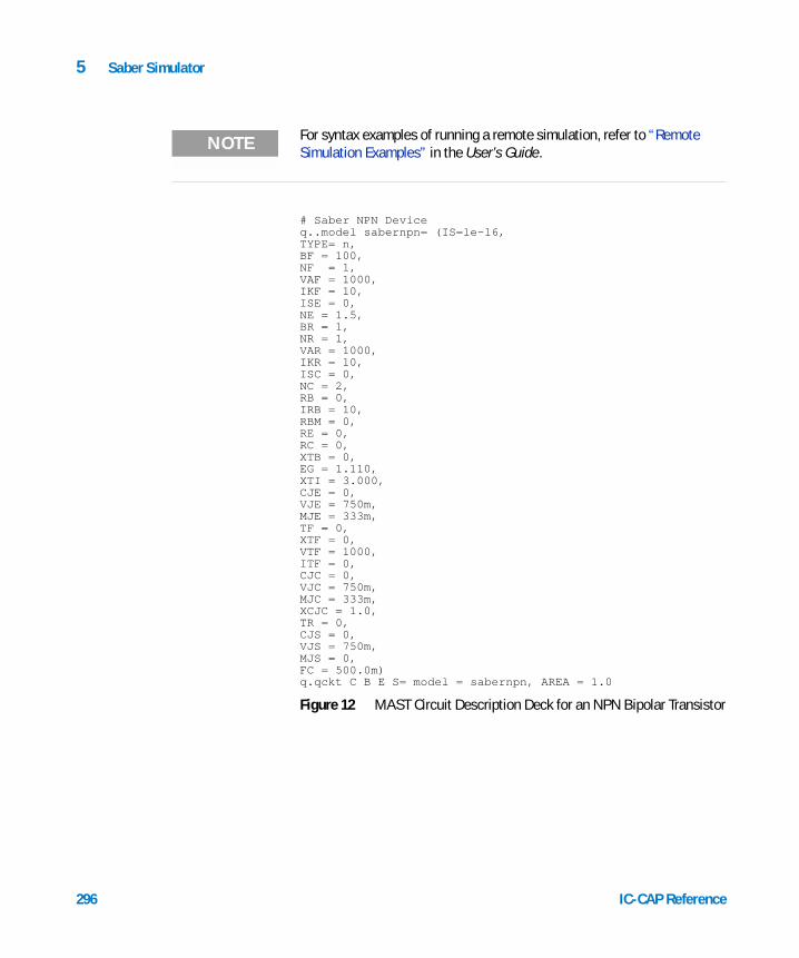
5 Saber Simulator
NOTE For syntax examples of running a remote simulation, refer to “Remote Simulation Examples” in the User’s Guide.
296
# Saber NPN Deviceq..model sabernpn= (IS=le-16,TYPE= n,BF = 100,NF = 1,VAF = 1000,IKF = 10,ISE = 0,NE = 1.5,BR = 1,NR = 1,VAR = 1000,IKR = 10,ISC = 0,NC = 2,RB = 0,IRB = 10,RBM = 0,RE = 0,RC = 0,XTB = 0,EG = 1.110,XTI = 3.000,CJE = 0,VJE = 750m,MJE = 333m,TF = 0,XTF = 0,VTF = 1000,ITF = 0,CJC = 0,VJC = 750m,MJC = 333m,XCJC = 1.0,TR = 0,CJS = 0,VJS = 750m,MJS = 0,FC = 500.0m)q.qckt C B E S= model = sabernpn, AREA = 1.0
Figure 12 MAST Circuit Description Deck for an NPN Bipolar Transistor
IC-CAP Reference

Saber Simulator 5
Piped and Non-Piped Saber Simulations
IC-CAP Reference
Non-piped Saber simulations are identical to non-piped SPICE simulations. However, there are differences between the 2 types of piped simulation. A piped simulation in Saber does the following:
1 Read the input deck from a file upon start up of the simulator
2 Read in the analysis commands from a pipe connected to standard input
3 Perform the simulation
4 Send the text output to a pipe connected to standard output
5 Save the output data to files
Saber is restarted if any topological changes are made to the circuit description. If changes are made which do not affect the topology of the circuit, such as changed parameter values, then alter commands are used and the simulator is not restarted.
NOTE The path of the AIM shell interpreter (aimsh) must be specified in usersimulators. IC-CAP uses this utility from the saber installation to interpret the simulation results and read them into IC-CAP. (AIM is a high-level, embedded scripting language that controls and manages user input and other kinds of analyses and processes in SaberDesigner applications.) The default saber specification in $ICCAP_ROOT\iccap\lib\usersimulators is as follows:
saber saber $SABER_HOME/bin/saber "" CAN_PIPE "" $SABER_HOME/bin/aimsh
Therefore, no modifications to usersimulators are required if SABER_HOME is properly set in your environment before launching IC-CAP.
297

298
5 Saber Simulator
Syntax: Non-Piped simulations
This section describes the argument syntax required to invoke the template simulator. This information is needed when writing the user translation module, since these are the arguments supplied by IC-CAP when it calls the translation module. For information on the translation module and adding a simulator, refer to “Adding a Simulator” in the User’s Guide.
The command format for a Saber non-piped simulation is as follows: saber -b deckfile
where:
-b specifies batch mode.
deckfile is the input file name. Saber will read deckfile as the input deck file containing the circuit description and deckfile as the command file containing the analysis statements.
The textfile is written to a file called deckfile.out.
The rawfile information is written to 2 files, called the control file and the data file. The control file is named deckfile.p1.suffix and the data file is named deckfile.p2.suffix where suffix is a keyword assigned by Saber according to the analysis being performed. Refer to the Saber User’s Manual for more information.
Syntax: Piped simulations
The command format for a Saber piped simulation is as follows: saber -c deckfile
where:
-c specifies the Saber command mode.
deckfile is the input deck file containing the circuit description.
Saber reads the analysis commands through standard input.
The textfile is written to a file called <deckfile>.out.
IC-CAP Reference

Saber Simulator 5
IC-CAP Reference
The rawfile is written to a file called <deckfile>.p1.<suffix> where suffix is a keyword assigned by Saber according to the analysis being performed. Refer to the Saber User’s Manual for more information.
299

5 Saber Simulator
Saber Parameter Sweeps
NOTE The LSYNC sweep is not supported with the Saber simulator.
300
When using the Saber simulator, IC-CAP allows parameter sweeps of only parameters and Saber global variables, such as the global variable for temperature called TEMP. Like SPICE-type simulators, specifying parameter sweeps for devices and circuits is done the same way. Parameter names must be entered in the Name field of the Input table exactly as they appear in the Parameters table. An input for vto, with Mode set to P, is added to the nmos2/short/idvd setup, as shown in the following figure.
The following figure shows the resulting plot.
Figure 13 Saber Parameter Sweep Setup Example
IC-CAP Reference
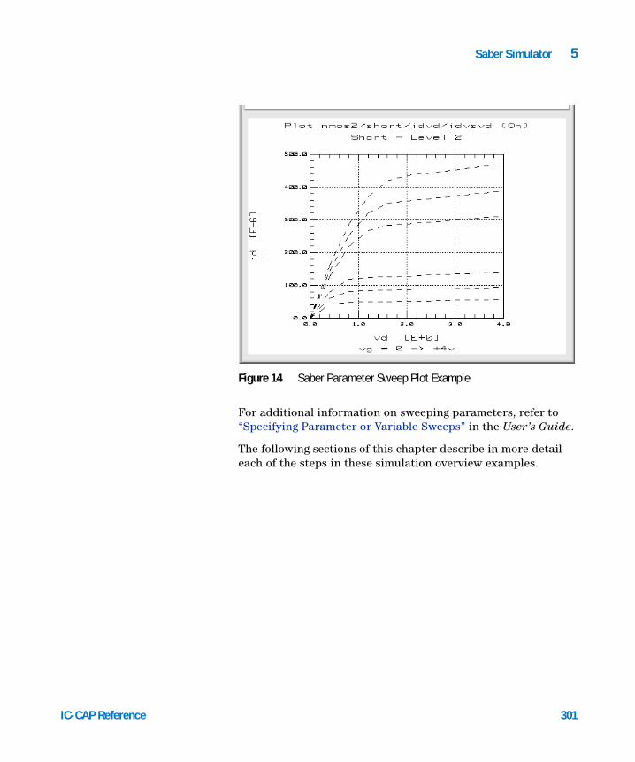
Saber Simulator 5
IC-CAP Reference
For additional information on sweeping parameters, refer to “Specifying Parameter or Variable Sweeps” in the User’s Guide.
The following sections of this chapter describe in more detail each of the steps in these simulation overview examples.
Figure 14 Saber Parameter Sweep Plot Example
301

5 Saber Simulator
The Alter Command
302
An alter command temporarily changes the value of any element or parameter in a MAST template. It is used to make a change in a template description so that a simulation can be re-executed without reloading the original circuit. The alter command cannot be used to make a change that modifies the topology of a design.
Alter commands are used in IC-CAP Saber simulations when the Circuit Description and Setup information, other than the sweep limits, remain unchanged from the previous simulation.
If only parameter values in the Device Parameters table or Model Parameters table are changed, IC-CAP will not restart the Saber simulator and reload the circuit. Instead, IC-CAP generates alter commands for every parameter, then re-executes the simulation commands. The USE_ALTER variable can be specified and set to No to override this behavior. In this case, Saber is restarted with every simulation whether or not the Circuit Description or Setup was changed. If the USE_ALTER variable does not exist, IC-CAP behaves as if the variable were set to Yes.
After a successful simulation, if a resistor is changed from a non-zero to zero value, Saber collapses the nodes. This causes an implicit topological change in the circuit that is not recognized by IC-CAP since the Circuit Description or Setup information has not been changed. Turn the USE_ALTER variable off by setting it to NO to allow IC-CAP to restart the Saber simulator and reload the altered circuit.
IC-CAP Reference

Saber Simulator 5
Circuit Model Description
IC-CAP Reference
This section discusses the circuit description for the Saber simulator.
Selecting Simulator Options
Saber simulation options are not specified in the circuit description, but rather in the analysis command line. Saber simulator options are set using the SABER_OPTIONS variable in the Setup, DUT or System variable tables.
Enter the options in the Value section of the variable exactly as they should appear in the Saber command string. For example, to perform a transient simulation from 0 to 0.8 nsec in 10 psec steps, the Saber command generated in IC-CAP is:tr(ts le-11, te 8e-10, tb 0)
To specify that all step sizes be fixed instead of variable, append the following option to the Saber command:steps fix
To do this in IC-CAP, specify the options command steps fix in the value field of the SABER_OPTIONS variable. Simulation now performs the following transient analysis command:tr(ts le-11, te 8e-10, tb 0, steps fix)
The SABER_OPTIONS variable can be specified in a variable table at any level. However, it is important to note that a SABER_OPTIONS variable specified in the DUT, Model or System variable tables is used by all simulations executed below that level. For example, if a SABER_OPTIONS variable is specified in the DUT variable table, every Setup under that DUT will use the specified option. This may result in simulation errors because 1 particular option may not be valid for every type of analysis being specified in the DUT.
Any number of options can be specified in the SABER_OPTIONS variable; they must be separated by a comma.
303

304
5 Saber Simulator
A Saber analysis in IC-CAP is always preceded by a DC operating point analysis. This DC command can also contain options and can be specified using the SABER_DC_OPTIONS variable.
Refer to Saber manuals for available options and corresponding syntax for each simulation type. Invalid options entered into the SABER_DC_OPTIONS and SABER_OPTIONS variables cause the simulation to fail.
Entering Circuit Descriptions
Circuit descriptions contain templates of devices and components, as well as node connections and model descriptions written in the MAST modeling language. All model parameter names must be specified when defining models. Circuit descriptions can also be read into the IC-CAP Circuit Editor from a file that already contains a description. You must enter circuit descriptions using valid model names and valid parameter names for the particular model being used.
Enter circuit descriptions for a Saber input deck with the Circuit Editor. IC-CAP contains a parser for descriptions written in the MAST modeling language.
There are 2 types of Saber circuit editor descriptions: devices and templates. Syntax rules for each type are described in the following sections.
Device Model Descriptions
A device model is used to characterize a single element of any type. This element can be predefined in the Saber library or defined by the user using the MAST modeling language.
A device model description requires a model definition written in the MAST modeling language and an element statement that calls a defined model.
IC-CAP Reference

Saber Simulator 5
IC-CAP Reference
A model description specifies the values of a device model that describes a particular element. When a parameter is not specified, the default value in the model template is used and the parameter does not appear in the IC-CAP Parameters table. The general form of the model definition is:ENAME..model MNAME = (PNAME1=PVAL1, PNAME2=PVAL2, ...PNAMEX=PVALX)
where
ENAME is the name of the element template
MNAME is the user-specified name of the model being defined
PNAME is a parameter name for the particular model type
PVALs are the corresponding parameter values
The general form of the element statement that calls the device model is:ENAME.DNAME NNAME1 NNAME2 ...NNAMEN = model = MNAME, DPAR1 = DVAL1, DPAR2 = DVAL2 ...DPARN = DVALN
where
ENAME is the element template name
DNAME is the device name
NNAME specifies a node name
MNAME is the name of the model being referenced
DPAR is a predefined DUT parameter name
DVAL is the corresponding DUT parameter value
A sample element statement in the MAST modeling language is: q.qckt C B E S = model = sabernpn,AREA = 1.0
where
q is the element template name defined in the Saber component library
qckt is the user-specified device name
C, B, E, and S are the node names
305

306
5 Saber Simulator
sabernpn is the model name. The model corresponding to this model name must be defined in the circuit description before the reference is made.
AREA is a DUT parameter of this model with an assigned value of 1.0
As in Saber, a line ending with a comma is continued on the next line.
Template Descriptions
A template is used to characterize a circuit that contains more than 1 device. The syntax for defining a template is identical to that of the MAST modeling language. A template can be defined as either an element template or a model template. The general form of the first line of a template element definition is:element template TEMPNAME NNAME1 NNAME2 ...NNAMEN = PAR1,PAR2, ...PARN
where
TEMPNAME is the template name
NNAME is a node name of the external node of the template. External nodes are used to connect the template to another circuit.
PAR is the name of the parameter passed into the template
The general form of the first line of a template model definition is:element template TEMPNAME NNAME1 NNAME2 ...NNAMEN = model
where
TEMPNAME is the template name
NNAME is the node name of the external node of the template. External nodes are used to connect the template to another circuit.
The body of a model definition defines the model parameters. For more information on writing templates, refer to the Saber MAST Reference manual.
IC-CAP Reference

Saber Simulator 5
IC-CAP Reference
When writing a template for model development within IC-CAP, the recommended procedure is to define the template in an external file and include this file in the IC-CAP circuit description using the MAST nomenclature <filename> to include a file. This minimizes the changes to be made in the IC-CAP Circuit Description and thereby increases the rate of model development because changes in the external template file will immediately be recognized in IC-CAP.
Non-Numeric Parameter Values
Saber allows non-numeric values for a number of parameters in predefined templates. The MOS model parameter type is 1 example. This parameter can take on the value of _n for an nmos device and _p for a pmos device.
When a Saber input parameter is in alpha format, it does not appear in the IC-CAP Parameters table but is still present in the input deck and passed to the simulator for analysis.
Node Names
Saber accepts alphanumeric names as well as numbers to represent nodes. There is no limit to the number of characters allowed in a node name (the command line has a limit of 1024 characters).
Test Circuits and Hierarchical Simulations
When characterizing a circuit, it is often necessary to add circuitry around a circuit or device to model the actual measurement Setup. IC-CAP provides a Test Circuit Editor to allow modeling of this additional bias circuitry. Select the DUT from the DUT/Setup panel. Click the Test Circuit tab and enter the test circuit description in the same manner you would enter a Circuit Description. The test circuit definition should include a call to the device or template
307

308
5 Saber Simulator
circuit defined in the Circuit Editor, as well as the additional circuitry needed to model the external parasitics of the measurement Setup.
NOTE When you define a test circuit, the DUT Parameters table contains the values specified in the test circuit specification. Regardless of the name entered in the TEMPNAME field of the template definition statement, IC-CAP uses the name of the DUT being simulated when the simulator input deck is built.
Template circuit and device model specifications can be called from inside another Model. This allows you to perform hierarchical simulations to study a circuit at different levels. For example, assume you have defined 3 Models, model1, model2, and model3. Model1 has a circuit model description that is a device definition. The circuit model description for model2 is a template circuit definition at the gate level that includes a call to model1 in a device call statement. And, the circuit model description for model3 is a template circuit definition that includes a call to model2 in a subcircuit call statement. When you simulate a Setup in model3, IC-CAP traverses the Model hierarchy and uses the circuit model description defined in model3, which includes calls to model1 and model2. The syntax for calling a device model is identical to that described in the Device Model Specifications section above.
The general form of the device call is: ENAME.DNAME NNAME1 NNAME2 ...NNAMEN = model MNAME, DPAR1 = DPAR1, DPAR2 = DVAL2 ...DPARN = DVALN
Calling a template specification allows you to insert an entire template into a circuit as if it were a single component. The call requires a syntax identical to that used in the MAST modeling language. The general form of the template element call is: TEMPNAME.TNAME NNAME1 NNAME2 ...NNAMEN = TPAR1 = TPARVAL1,TPAR2 = TPARVAL2, ...TPARN = TPARVALN
where
IC-CAP Reference

Saber Simulator 5
IC-CAP Reference
TEMPNAME is the name of the template previously described by a template definition. This template definition could exist in a different Model.
TNAME is the user specified name given to this particular instance of the template described by TEMPNAME.
NNAMEs represent the node names of the calling circuit that connect to the external nodes of the template. The calling circuit’s node names need not be the same as the external nodes of the template. The order in which you specify these nodes is the order in which they are connected. The same number of nodes as declared in the template definition must be specified.
TPARs are predefined template parameter names. These parameters are defined in the template definition. TPARVALs are the corresponding values of the template parameters.
A hierarchical simulation, in which a template in 1 model references a device defined in a different model, requires the use of a MAST external declaration in the template definition. For example, assume a MOS device model (Saber template m named nmos2), which is called in the body of a circuit template called inverter in another model. This inverter template must include the following declaration in order for the nmos2 device model to be recognized. external m..model nmos2
The complete template for the inverter circuit is:template inv A B C D E Felectrical A, B, C, D, E, F{external m..model nmos2m.minv A B C D = model = nmos2, l = 10u, w = 10um.mload E F A D = model = nmos2, l = 10u, w = 10u}
The external declaration does not need to be added when a template calls another template.
Refer to the Saber manuals for complete syntax and rules of the MAST modeling language.
309

310
5 Saber Simulator
Saber Libraries
The Saber library of components and templates includes the SPICE components as well as the components developed by Analogy, Inc. Refer to the Saber manuals for a list of supported simulator components, higher level templates and the required specification formats.
Saber Input Deck Comments
To indicate comments in the Saber simulator input deck, start an input line with the pound symbol (#). This denotes a comment in the circuit model description or in the input file of the Simulation Debugger.
NOTE The SABER_DATA_PATH environment variable must be set. This variable contains the directory paths for the executable files and libraries required by the Saber simulator. Refer to the Saber Reference Manual for installation procedures.
IC-CAP Reference

Agilent 85190A IC-CAP 2008Reference
6MNS Simulator
MNS Simulation Example 313
Piped MNS Simulations 316
Non-Piped MNS Simulations 317
MNS Parameter Sweeps 318
Circuit Model Description 323
MNS Input Language 328
MNS Libraries 328
This chapter describes the details of using the MNS simulator with IC-CAP. For general information on IC-CAP simulation, refer to Chapter 6, “Simulating,” in the User’s Guide.
IC-CAP supports the following Microwave Nonlinear Simulator (MNS) features:
• DC, Small Signal AC, Small Signal S-Parameter, and Transient analysis options
• Parameter sweeps for device and circuit simulation
• Temperature sweeps
• Hierarchical simulation
• Variables
• Constants
• Expressions
The MNS Optimizer features are not currently supported in IC-CAP. IC-CAP optimization (different from the MNS Optimizer) of simulated data to target data is supported.
311Agilent Technologies

312
6 MNS Simulator
The MNS simulator supports the following analysis types:
• DC
• AC
• 2-port
• Transient
• Noise
• Capacitance Voltage (CV)
• Time-Domain Reflectometry (TDR)
• Harmonic Balance
NOTE IC-CAP does not add extra circuitry in order to perform a 2-port simulation since this is a standard type in MNS.
IC-CAP Reference

MNS Simulator 6
MNS Simulation Example
IC-CAP Reference
The circuit description is predefined for all IC-CAP configuration files. Enter this description if a new model is being defined; edit the description to fit specific needs. The syntax is identical to the syntax used for describing circuits in a typical MNS simulation deck.
This MNS simulation example will use the IC-CAP supplied Model mnsnpn.mdl.
1 Select the simulator by choosing Tools > Options > Select Simulator > mns. Choose OK.
2 Choose File > Open > mnsnpn.mdl. Choose OK.
3 View the description by clicking the Circuit tab.
The circuit description is shown in the following figure. This deck describes the circuit (in this case, a single device) to be used in the simulation.
4 To view the input and output for the fearly setup, click the DUTs-Setups tab and select fearly.
options ascii=nomodel npnbjt bjt NPN=yes \IS=4.015e-16 BF = 87.01 \NF = 0.9955 VAF = 84.56 \IKF = 0.01195 ISE = 3.405E-14 \NE = 1.594 BR = 10.79 \NR = 1.002 VAR = 9.759 \IKR = 0.0237 ISC = 1.095E-15 \NC = 1.1 RB = 9.117 \IRB = 0.001613 RBM = 5.62 \RE = 1.385 RC = 9.292 \XTB = 1.7 EG = 1.11 \XTI = 3 CJE = 1.312E-12 \VJE = 1.11 MJE = 0.3475 \TF = 5.274E-11 XTF = 5.625 \VTF = 2.678 ITF = 0.02382 \PTF = 154.1 CJC = 1.396E-12 \VJC = 0.4511 MJC = 0.1924 \XCJC = 0.3 TR = 1E-09 \CJC = 9.985E-14 VJS = 0.8137 \MJS = 0.3509 FC = 0.5 npnbjt:qckt C B E S
Figure 15 MNS Circuit Description Deck for an NPN Bipolar Transistor
313
314
6 MNS Simulator
The Measure/Simulate folder appears with the inputs vb, vc, ve, and vs, and the output ic. The vc input specifies a voltage source at node C that sweeps linearly from 0 to 5V in 21 steps. The ic output specifies that current at node C be monitored.
In the Plots folder, icvsvc is specified so that the results of the simulation can be viewed graphically.
5 To simulate, click the Simulate button in the Measure/Simulate folder. The Status line displays Simulate in progress.
When the simulation is complete, the Status line displays IC-CAP Ready.
6 To view the results of the simulation, display the Plots folder and click Display Plot. The plot displays measured data represented by solid lines and simulated data represented by dashed lines.
The Simulation Debugger
NOTE Phase information from the sin input cannot be included in the netlist.
NOTE For syntax examples of running a remote simulation, refer to “Remote Simulation Examples” in the User’s Guide.
When using MNS with the Simulation Debugger to perform an IC-CAP simulation (as opposed to a manual simulation), an output text file consists of only the computational analysis information. An example of a typical AC analysis output text file is as follows: MNS (ver. 03.00 -- 12 Feb 2004)Copyright Agilent Technologies, 2004AC ac1[1] <baaa07774> freq=(1 kHz->10 MHz)Time required for ac1[1] was 0.30 seconds.
IC-CAP Reference

MNS Simulator 6
IC-CAP Reference
This file does not include the resulting data. To generate a more informative output text file, change the ascii option in the Input File from ascii=no to ascii=yes and perform a manual simulation. An output text file that includes the simulated output data values is produced. The ascii option is set to no by IC-CAP before every simulation so that the binary raw data file is generated by MNS. IC-CAP needs the binary raw data file to read the resulting simulation data. However, this data is not needed for a manual simulation.
MNS version 4.0 requires that the option nutmeg be set to yes to cause MNS to generate the binary raw data file required by IC-CAP. If the nutmeg option is not specified, the default is nutmeg = yes. If you set nutmeg = no, MNS will generate an output data format that IC-CAP cannot understand.
315

6 MNS Simulator
Piped MNS Simulations
316
Specifying CAN_PIPE (the default) in your usersimulators file for MNS enables IC-CAP to take advantage of the tune mode built into the MNS simulator. This mode permits changing parameters of a simulation without requiring the simulator to be relaunched. This greatly reduces the time required for an optimization which has all simulated targets within 1 setup. Whenever the setup is changed, the simulator is stopped and restarted with the new resulting netlist. Thus, an optimization that has multiple simulated targets from different setups must stop the simulator and restart it at each iteration as it switches between setups. The performance of this second scenario is the same as if the non-piped mode were used.
IC-CAP Reference

MNS Simulator 6
Non-Piped MNS Simulations
IC-CAP Reference
Non-piped MNS simulations are identical to non-piped SPICE simulations. Execute a simulation with the Simulation Debugger ON to perform a non-piped simulation. MNS is capable of performing piped simulations, which enables you to turn the Simulation Debugger OFF without requiring that MNS be restarted for every simulation.
Syntax: Non-piped simulation
This section describes the argument syntax required to invoke the template simulator. This information is needed when writing the user translation module, since these are the arguments supplied by IC-CAP when it calls the translation module. For information on the translation module and adding a simulator, refer to “Adding a Simulator” in the User’s Guide.
The command format for an MNS non-piped simulation is as follows: mns -r rawfile deckfile
where:
deckfile is the input deck file containing the circuit description and analysis commands.
rawfile is the output binary data file.
The output text file, which normally is sent to standard output is redirected by IC-CAP to a file. This file is displayed in the Output table of the Simulation Debugger if it is on.
317

6 MNS Simulator
MNS Parameter Sweeps
318
When using the MNS simulator in IC-CAP, the method of specifying parameter sweeps differs between performing single device simulations and circuit simulations.
NOTE When performing parameter sweeps, the name of the parameter to be swept must be recognized by MNS, since the analysis is performed from within the simulator. This means that the global declaration must be used within the MNS circuit description. Simply adding the parameter name to the Variables table results in a failed simulation.
Device Simulation Parameter Sweep
To sweep a parameter in an MNS device simulation:
1 Add an input specification of mode P to the Setup. Enter the name of the parameter as it appears in the Parameters table.
2 Enter the sweep type and values.
The Device Simulation Parameter Sweep example uses the mnsnpn.mdl model with an input of mode P to the fearly setup. This input specifies a linear sweep of the parameter from 200.0e−15 to 230.0e−15 amperes in steps of 15.0e−15 amperes.
Figure 16 MNS Device Simulation Parameter Sweep Setup Example
IC-CAP Reference

MNS Simulator 6
IC-CAP Reference
During the simulation, IC-CAP generates the following input deck.; Simulation Input File options ascii=no model mnsnpn bjt npn=yes\is=4.015E-16\ bf = 60 \ nf = 0.9955\ vaf = 84.56\ ikf = 0.01195 \ ise = 3.405E-14 \ ne = 1.594 \ br = 10.79 \ nr = 1.002 \ var = 9.759 \ ikr = 0.00237 \ isc = 1.095E-15 \ nc = 1.1 \ rb = 9.117 \ irb = 0.001613 \ rbm =5.62 \ re = 1.385 \ rc = 9.292 \ xtb = 1.7 \ eg = 1.11 \ xti = 3 \ cje = 1.312E-12 \ vje = 1.11 \ mje = 0.3475 \ tf = 5.274E-11 \ xtf = 5.625 \ vtf = 2.678 \ itf = 0.02382 \ ptf = 154.1 \ cjc = 1.396E-12 \ vjc = 0.4511 \ mjc = 0.1924 \ xcjc = 0.3 \ tr = 1E-09 \ cjs = 9.985E-14 \ vjs = 0.8137 \ mjs = 0.3509 \ fc = 0.5mnsnpn:devckt 1 2 3 4 \area = 1; START SOURCESivs:V2GROUND 2 0 vdc=0ivs:V1GROUND 3 0 vdc=0ivs:V3GROUND 3 0 vdc=0ivs:V4GROUND 4 0 vdc=0; END SOURCESstim:swp1 start=0 stop=5 step=0.25stim:swp2 start=0.7 stop=0.72 step=0.01stim:swp3 start=200a stop=230a step=15adc:dc1 stim=swp1 var="V1GROUND.vdc"ct:ct1 an="dc1" stim=swp2 var="V2GROUND.vdc"ct:ct2 an="ct1" stim=swp3 var="mnsnpn.is"
319

320
6 MNS Simulator
Circuit Simulation Parameter Sweep
Specifying a parameter sweep for a circuit simulation requires a different approach from a parameter sweep for a device simulation.
To sweep a parameter in an MNS circuit simulation:
1 Specify a global variable in the MNS circuit description and set it to an initial value.
2 Set the value of the parameter in the circuit description equal to the global variable name.
3 Add a variable in IC-CAP with the same name as the global MNS parameter.
4 Add an input specification of mode P to the Setup.
5 Enter the global variable name in the Name field of the Input table.
6 Enter the sweep type and values.
IC-CAP Reference

MNS Simulator 6
Example Circuit Simulation Parameter Sweep
IC-CAP Reference
The Circuit Simulation Parameter Sweep example, uses the model mnsopamp.mdl. The following line is added to the circuit description:
global RC1_r=4352
This complete circuit description is shown below. ; Simulation Input File in MNS Input Deck Formatoptions ascii=no define opamp1 (2 3 4 6 7 )global RC1_r=4352;Internal OpAmp circuit;using Boyle-Pederson Macro Model;Input differential amplifiernpn1:Q1 10 2 12npn2:Q2 11 3 13model npn1 bjt npn=yes is = 8E-16 bf = 52.81model npn2 bjt npn=yes is = 8.093E-16 bf = 52.66r:RC1 7 10 r=RC1_rr:RC2 7 11 r=4352c:C1 10 11 c=4.529E-12r:RE1 12 14 r=2392r:RE2 13 14 r=2392r:RE 14 0 r+7.27E+06c:CE 14 0 c=7.5E-12; Power dissipation modeling resistorr:RP 7 4 r=1.515E+04; 1st gain stagevccs:GCM 0 15 14 0 gm=1.152E-09vccs:GA 15 0 10 11 gm=0.0002298r:R2 15 0 r=1E+05; Compensation capacitorc:C2 15 16 c=1E-11; 2nd gain stagevccs:GB 16 0 15 0 gm=37.1r:RO2 16 0 r=489.2dmod1:D1 16 17dmod1:D2 17 16model dmod1 diode is = 3.822E-32r:RC 17 0 r=0.0001986vccs:GC 0 17 6 0 gm=5034; Output circuitr:RO1 16 6 r=76.8dmod2:D3 6 18dmod2:D4 19 6model dmod2 diode is = 3.822E-32ivs:VC 7 18 vdc=1.604ivs:VE 19 4 vdc=3.104; Input diff amp bias sourceics:IEE 14 4 idc=2.751E-05end opamp1
In this example, the value of r:RC1 is set to RC1_r. You must also add a variable called RC1_r to the IC-CAP model variables table and set the variable to a value, such as,
321

322
6 MNS Simulator
4.000K. In the setup mnsopamp/inv_amp/B_P_macro add an input called RC1_r. The Inputs table is shown in the following figure.
For additional information on sweeping parameters, refer to “Specifying Parameter or Variable Sweeps” in the User’s Guide.
The following sections of this chapter describe in more detail each of the steps in these simulation overview examples.
Figure 17 MNS Circuit Parameter Sweep Setup Example
IC-CAP Reference

MNS Simulator 6
Circuit Model Description
IC-CAP Reference
This section explains the circuit descriptions for the MNS simulator.
Selecting Simulator Options
MNS simulation options are specified using the MNS_OPTIONS variable in the Setup DUT or System Variable tables. Enter the options in the value section of the variable exactly as they should appear in the MNS options command.
Entering Circuit Descriptions
The circuit description is entered into the IC-CAP Circuit Editor or the Test Circuit Editor. The circuit description includes the necessary definitions of devices, sources and components, as well as node connections and model descriptions. MNS accepts a netlist description that is different from SPICE and Saber simulators.
Parameter Table Generation
The circuit description is parsed by IC-CAP and specific model information (such as parameters and their corresponding values) as well as circuit component values are reflected in the Parameters table. Model parameters and component values specified in the circuit description entered in the Circuit Editor are saved in the Parameters table. Device parameters specified in the model call statement are saved in the DUT Parameters table—unless a Test Circuit is specified, in which case, parameter values specified in the test circuit description are saved in the DUT Parameters table.
Non-numeric Parameter Values
MNS allows non-numeric values for a number of parameters in predefined component definitions. One example is the BJT model parameter npn. This parameter can take on the value
323

324
6 MNS Simulator
of yes if it is an nmos device. Alpha format parameters do not appear in the IC-CAP Parameters table but do appear in the simulation input decks.
Circuit descriptions must be entered with valid model and parameter names for the particular model being used.
Node Names
MNS accepts alphanumeric names as well as numbers to represent nodes. There is no limit on the number of characters allowed in a node name; however, delimiters or non-alphanumeric characters are not allowed. Also, a node name that begins with a digit must consist only of digits.
Comments
To indicate comments in an MNS input deck, start an input line with a semicolon (;). All text on the line following the semicolon will be ignored.
Device Model Descriptions
NOTE MNS will treat the suffix M as MEG and m as milli, whereas IC-CAP parses both M and m as milli. When specifying a value multiplied by10-3 use m; when specifying a value multiplied by 106 use MEG.
A device model is used to characterize a single MNS-defined element of any type. This specification requires a model definition that describes the device and an instance statement that calls the model definition.
The model description specifies the value of a device model that describes a particular element. When a parameter is not specified, the default value in the model is used. The general form of the model definition is: model MNAME TYPE PNAME1 = PVAL1 PNAME2 = PVAL2...
where
IC-CAP Reference

MNS Simulator 6
IC-CAP Reference
MNAME is the model name. (Regardless of the model name entered into the MNAME field of the MNS model definition statement, IC-CAP substitutes this field with the name of the Model as it is called in the Model List when the simulator input deck is built.)
TYPE is a valid MNS element type.
PNAMEs are parameter names available for the particular model type.
PVALs are the parameter values.
A backslash immediately followed by a return (no space between the backslash and the return) at the end of a line indicates that the statement is continued on the next line This continuation character is often used for easier readability when specifying the model description.
The general form of the instance statement that calls the device model is:TYPE :DNAME NNAME1 NNAME2...NNAMEN DPAR1 = DVAL1 DPAR2 = DVAL2...DPARN = DVALN
where
TYPE is the instance type descriptor. This field can contain either the MNS instance type name or a user-supplied model or subcircuit name.
DNAME is the device name.
NNAMEs denote node names.
DPAR is a predefined DUT parameter name.
DVAL is the specified DUT parameter value. Refer to the MNS User’s Guide for DUT parameter names available for each model.
Subcircuit Model Descriptions
A subcircuit definition represents a circuit that contains more than 1 device. The syntax for defining a subcircuit is identical to the syntax used for the MNS input language.
The general form of the subcircuit definition is:
325

326
6 MNS Simulator
define SUBCKTNAME (NNAME1 NNAME2 ...NNAMEN)parameters PAR1 = VAL1 PAR2 = VAL2 ...PARN = VALN< body of subcircuit >end SUBCKTNAME
where
SUBCKTNAME is the name of the subcircuit.
NNAMEs are the node names of the external nodes of the subcircuit. These external nodes are used to connect the subcircuit to another circuit.
PARs are the names of the parameters passed into the subcircuit. These parameters are optional in a subcircuit definition.
If parameters are specified, the assigned default values VAL are also optional. A parameter is assigned to this default value if the parameter is not specified in the subcircuit call.
The body of the subcircuit contains element statements. It can contain calls to other subcircuits but it cannot contain other subcircuit definitions.
The subcircuit definition is completed using the end SUBCKTNAME statement.
Calling a subcircuit definition allows you to insert all instances specified within the subcircuit into the circuit. The call requires a syntax identical to the syntax used in the MNS input language for any instance statement. The general form of the instance statement is: TYPE :INAME NNAME1 NNAME2....NNAMEN PAR1 = VAL1 PAR2 = VAL2......PARN = VALN
(While the syntax shown here is correct, passed parameters are ignored by IC-CAP.)
where
TYPE is the instance type descriptor. If a subcircuit is being called, this field would contain the subcircuit name denoted by SUBCKTNAME.
INAME is the instantiated name of the subcircuit.
NNAMEs denote node names.
IC-CAP Reference

MNS Simulator 6
IC-CAP Reference
PARs are the subcircuit parameter names.
VALs are the specified subcircuit parameter values.
The following is an example of a complete subcircuit definition and subcircuit call.
• Defined by the user in the Circuit folder:options ascii=no define opamp1 (2 3 4 6 7); Internal OpAmp circuit; using Boyle-Pederson Macro Model; Input differential amplifiernpn1:Q1 10 2 12npn2:Q2 11 3 13model npn1 bjt npn=yes is = 8E-16 bf = 52.81model npn2 bjt npn=yes is = 8.093E-16 bf = 52.66r:RC1 7 10 r=4352r:RC2 7 11 r=4352c:C1 10 11 c=4.529E-12r:RE1 12 14 r=2392r:RE2 13 14 r=2392r:RE 14 0 r=7.27E+06c:CE 14 0 c=7.5E-12: Power dissipation modeling resistorr:RP 7 4 r=1.515E+04: 1st gain stagevccs:GCM 0 15 14 0 gm=1.152E-09vccs:GA 15 0 10 11 gm=0.0002298r:R2 15 0 r=1E+05; Compensation capacitorc:C2 15 16 c=1E-11; 2nd gain stagevccs:GB 16 0 15 0 gm=37.1r:RO2 16 0 r=489.2dmod1:D1 16 17dmod1:D2 17 16model dmod1 diode is = 3.822E-32r:RC 17 0 r=0.0001986vccs:GC 0 17 6 0 gm=5034; Output circuitr:RO1 16 6 r=76.8dmod2:D3 6 18dmod2:D4 19 6model dmod2 diode is = 3.822E-32ivs:VC 7 18 vdc=1.604ivs:VE 19 4 vdc=3.104; Input diff amp bias sourceics:IEE 14 4 idc=2.751E-05end opamp1
327
328
6 MNS Simulator
• Defined by the user in the Test Circuit folder:;Inverting Amplifierdefine inv_amp (1 2 3 4 6 7 )opamp1:X1 2 3 4 6 7r:Rf 6 2 r=1E+04r:Rin 2 1 r=2000r:Rgnd 3 0 r=0.001end inv_amp
• Added by IC-CAP to the circuit description:inv_amp:XCKT 1 2 3 4 5 6; START SOURCESivs:V1GROUND 10 vdc=0 vac=1 ivs:V7GROUND 6 0 vdc=15ivs:V5GROUND 4 0 vdc=-15 ; END SOURCESr:RO2 2 0 100000r:RO3 3 0 100000r:RO5 5 0 100000stim:swpfreq start=1000 stop=1e=07 dec=3ac:ac1 stim=swpfreq var="freq"
For more information on MNS subcircuit definitions, refer to the MNS User’s Guide.
MNS Input Language
The MNS Input Language, which describes circuit and simulator control statements, is different from the SPICE Input Language and the Saber Input Language (MAST). For information about the MNS input language, refer to the MNS User’s Guide.
MNS Libraries
MNS contains a library of elements and components. For information about the MNS Libraries, refer to the MNS User’s Guide.
IC-CAP Reference

Agilent 85190A IC-CAP 2008Reference
7ADS Simulator
ADS Interfaces 332
Hardware and Operating System Requirements 333
Codewording and Security 333
Setting Environment Variables 334
ADS Simulation Example 335
Piped ADS Simulations 338
Non-Piped ADS Simulations 340
Circuit Model Description 340
ADS Parameter Sweeps 347
Interpreting this Chapter 354
General Syntax 357
The ADS Simulator Syntax 358
Instance Statements 366
Model Statements 367
Subcircuit Definitions 368
Expression Capability 370
VarEqn Data Types 392
“C-Preprocessor” 393
Data Access Component 396
Reserved Words 398
This chapter describes the details of using the Advanced Design System (ADS) Simulator with IC-CAP. For general information on IC-CAP simulation, refer to Chapter 6, “Simulating,” in the User’s Guide.
329Agilent Technologies
7 ADS Simulator
NOTE The PC version of IC-CAP supports ADS version 2002 or newer. Older versions of ADS can not be used with the PC version of IC-CAP.
330
IC-CAP supports the following ADS features:
• DC, Small Signal AC, Small Signal S-Parameter, and Transient analysis options
• Parameter sweeps for device and circuit simulation
• Temperature sweeps
• Hierarchical simulation
• Variables
• Constants
• Expressions
• Spectre circuit page
The ADS Optimizer features are not currently supported in IC-CAP. IC-CAP optimization (different from the ADS Optimizer) of simulated data to target data is supported.
The ADS simulator supports the following analysis types:
• DC
• AC
• 2-port
• Transient
• Noise
• Capacitance Voltage (CV)
• Time-Domain Reflectometry (TDR)
• Steady State Harmonic Balance
IC-CAP Reference

ADS Simulator 7
NOTE 2-port simulation with high frequency noise is supported to extract noise parameters such as noise figure, optimum source reflection coefficients, equivalent noise resistance data, minimum noise figure data, and equivalent noise temperature data.
IC-CAP does not add extra circuitry in order to perform a 2-port simulation since this is a standard type in ADS.
IC-CAP Reference 331

7 ADS Simulator
ADS Interfaces
332
IC-CAP provides two template names to interface to the ADS simulator’s Circuit and Test Circuit pages—hpeesofsim uses native ADS simulator syntax and spmodeads uses spectre simulator syntax. Both interfaces use native ADS simulator syntax to specify the sweep and output requests.
To specify the hpeesofsim or spmodeads interface, usersimulators should have a line similar to the following:hpeesofsim hpeesofsim $ADS_DIR/bin/iccapinterface "" CAN_PIPE
orspmodeads spmodeads $ADS_DIR/bin/iccapinterface "" CAN_PIPE
The first field can be any name you choose, it will show up in your simulator list, and it can be used with the SIMULATOR variable.
Both the hpeesofsim and spmodeads lines shown above are in the usersimulators file by default.
When using the spmodeads interface, refer to “Circuit Model Descriptions” on page 278 in Chapter 4, “SPECTRE Simulator” for spectre syntax for the Circuit and Test Circuit pages.
IC-CAP Reference

ADS Simulator 7
Hardware and Operating System Requirements
IC-CAP Reference
The ADS Simulator on IC-CAP is supported on the following platforms:
• Linux RedHat Enterprise 4.0 or Linux Novell SUSE SLES 9
• Solaris 10
• Microsoft Windows XP or Microsoft Windows Vista.
Codewording and Security
The ADS Simulator is a secured program that requires, at a minimum, a license for the E8881 Linear Simulator to run. Depending on the type of simulation, additional licenses may be required.
333

7 ADS Simulator
Setting Environment Variables
334
Before running the ADS Simulator, set the environment variable HPEESOF_DIR on UNIX or ADS_DIR on Windows to point to the ADS Simulator’s installation location.
• To set HPEESOF_DIR using the Korn Shell, add the following to your ~/.profile. export HPEESOF_DIR=<ADS_install_directory>
• To set HPEESOF_DIR using the C Shell, add the following to your ~/.cshrc. setenv HPEESOF_DIR <ADS_install_directory>
• To set ADS_DIR for Windows 2000, right click on My Computer and select Properties. Click on the Advanced tab. Then select Environment Variables and set ADS_DIR either for the local user or system wide, depending on your needs.
• To set ADS_DIR for Windows NT 4.0, right click on My Computer and select Properties. Click on the Environment tab. Then set ADS_DIR either for the local user or system wide, depending on your needs. You may need to log off and log back onto the computer for the new variable to be found by IC-CAP.
IC-CAP Reference
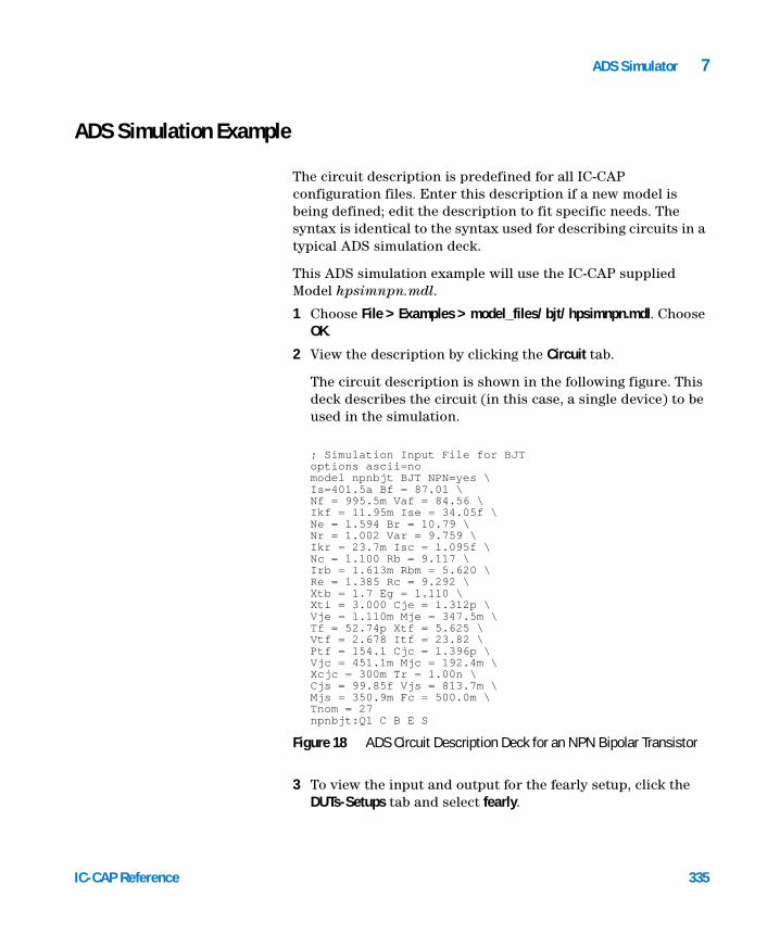
ADS Simulator 7
ADS Simulation Example
IC-CAP Reference
The circuit description is predefined for all IC-CAP configuration files. Enter this description if a new model is being defined; edit the description to fit specific needs. The syntax is identical to the syntax used for describing circuits in a typical ADS simulation deck.
This ADS simulation example will use the IC-CAP supplied Model hpsimnpn.mdl.
1 Choose File > Examples > model_files/bjt/hpsimnpn.mdl. Choose OK.
2 View the description by clicking the Circuit tab.
The circuit description is shown in the following figure. This deck describes the circuit (in this case, a single device) to be used in the simulation.
3 To view the input and output for the fearly setup, click the DUTs-Setups tab and select fearly.
; Simulation Input File for BJToptions ascii=nomodel npnbjt BJT NPN=yes \Is=401.5a Bf = 87.01 \Nf = 995.5m Vaf = 84.56 \Ikf = 11.95m Ise = 34.05f \Ne = 1.594 Br = 10.79 \Nr = 1.002 Var = 9.759 \Ikr = 23.7m Isc = 1.095f \Nc = 1.100 Rb = 9.117 \Irb = 1.613m Rbm = 5.620 \Re = 1.385 Rc = 9.292 \Xtb = 1.7 Eg = 1.110 \Xti = 3.000 Cje = 1.312p \Vje = 1.110m Mje = 347.5m \Tf = 52.74p Xtf = 5.625 \Vtf = 2.678 Itf = 23.82 \Ptf = 154.1 Cjc = 1.396p \Vjc = 451.1m Mjc = 192.4m \Xcjc = 300m Tr = 1.00n \Cjs = 99.85f Vjs = 813.7m \Mjs = 350.9m Fc = 500.0m \Tnom = 27npnbjt:Q1 C B E S
Figure 18 ADS Circuit Description Deck for an NPN Bipolar Transistor
335

336
7 ADS Simulator
The Measure/Simulate folder appears with the inputs vb, vc, ve, and vs, and the output ic. The vc input specifies a voltage source at node C that sweeps linearly from 0 to 5V in 21 steps. The ic output specifies that current at node C be monitored.
In the Plots folder, icvsvc is specified so that the results of the simulation can be viewed graphically.
4 To simulate, click the Simulate button in the Measure/Simulate folder. The Status line displays Simulate in progress. Under most configurations, the ADS status window will appear. For more information about these configurations, see “Piped ADS Simulations” on page 338.
When the simulation is complete, the Status line displays Simulate Complete.
5 To view the results of the simulation, right-click on fearly, then choose Plots > icvsvc. (This is a shortcut for displaying the plot from the Plots folder.) The plot displays measured data represented by solid lines and simulated data represented by dashed lines.
The Simulation Debugger
NOTE For syntax examples of running a remote simulation, refer to “Remote Simulation Examples" in the User’s Guide.
When using ADS with the Simulation Debugger to perform an IC-CAP simulation (as opposed to a manual simulation), an output text file consists of only the computational analysis information. An example of a typical AC analysis output text file is as follows:
IC-CAP Reference

ADS Simulator 7
HPEESOFSIM (ver. 03.00 -- 12/14/01 09:28:45)Copyright Agilent Technologies, 2004
CT ct1[1] </var/tmp/ICCAAa18727> VBGROUND.Vdc=(700 mV->720 mV)
DC ct1[1].dc1[1/3] </var/tmp/ICCAAa18727> VBGROUND.Vdc=700 mV VCGROUND.Vdc=(0 V->5 V)
DC ct1[1].dc1[2/3] </var/tmp/ICCAAa18727> VBGROUND.Vdc=710 mV VCGROUND.Vdc=(0 V->5 V)
DC ct1[1].dc1[3/3] </var/tmp/ICCAAa18727> VBGROUND.Vdc=720 mV VCGROUND.Vdc=(0 V->5 V)
-------------------Simulation finished.-------------------
IC-CAP Reference
This file does not include the resulting data. To generate a more informative output text file, change the ASCII_Rawfile option in the Input File from ASCII_Rawfile=no to ASCII_Rawfile=yes and perform a manual simulation. An output text file that includes the simulated output data values is produced. The ASCII_Rawfile option is set to no by IC-CAP before every simulation so that the binary raw data file is generated by ADS. IC-CAP needs the binary raw data file to read the resulting simulation data. However, this data is not needed for a manual simulation.
ADS version 1.3 requires that the option UseNutmegFormat be set to yes to cause ADS to generate the binary raw data file required by IC-CAP. If the UseNutmegFormat option is not specified, the default is UseNutmegFormat = yes. If you set UseNutmegFormat = no, ADS will generate an output data format that IC-CAP cannot understand.
337

7 ADS Simulator
Piped ADS Simulations
338
Specifying CAN_PIPE (the default) in your usersimulators file for the ADS simulator enables IC-CAP to take advantage of the tune mode built into the ADS simulator. This mode permits changing parameters of a simulation without requiring the simulator to be relaunched. This greatly reduces the time required for optimizations to run. However, each setup requires a new simulator to be launched. By default, IC-CAP permits up to 3 ADS simulators to be running at once so that an optimization across as many as 3 setups can be completed in the fastest time possible. Certain large simulations may require a great deal of system resources and having 3 simulations currently active can degrade system performance. If you encounter this problem, you can set the MAX_PARALLEL_SIMULATORS system variable to 1 or 2. If your system can handle more than 3 simulators in parallel and you need to optimize across more than 3 setups at a time, the value of MAX_PARALLEL_SIMULATORS can be increased.
When CAN_PIPE mode is used, the ADS simulator will bring up a status window during simulation. The first time the simulator is launched it can take several seconds for this window to appear. Once it is open, successive simulations will attach to the same status window. Each time a new setup is simulated, a new simulator must be started. There is a certain start-up delay associated with each invocation. This will be much shorter than the very first invocation which needed to launch the status window. Successive simulations of a setup which has been previously simulated will return in the shortest time as the simulator does not need to be reinvoked.
Opening the Simulation Debugger will terminate all running simulators, and close the ADS status window. Simulations done with the Simulation Debugger window open are performed in non-piped mode and thus the ADS status window is not opened.
In situations when you want to use the $mpar or $dpar feature in #echo lines for MNS and ADS netlists, you must enter names properly. The proper ADS name syntax is a dot-separated name, such as NPN.Bf. If you fail to use a proper name, simulations
IC-CAP Reference

ADS Simulator 7
IC-CAP Reference
will yield incorrect results when you try to use the simulator in CAN_PIPE mode. If names cannot be revised, use CANNOT_PIPE.
This was especially problematic for userdefined models requiring many #echo lines using the $mpar feature in order for IC-CAP to parse it properly. This problem occurs when the technique used to implement userdefined models in ADS is declaring 2 new components, 1 a modelform and another an instance. This implementation of user-defined models led to the requirement for #echo lines. The modelform component looked like any other ADS netlist component, but it had no nodes. The parser is modified for IC-CAP 2001 to recognize a nodeless component as a userdefined model; however, only in the context of a subcircuit. If you want to create this type of userdefined model in ADS, then you must use a subcircuit. Doing so eliminates the need for #echo lines in the netlist and the subcircuit will parse and simulate properly.
339

7 ADS Simulator
Non-Piped ADS Simulations
340
Non-piped ADS simulations are identical to non-piped MNS simulations. Execute a simulation with the Simulation Debugger ON to perform a non-piped simulation. ADS is capable of performing piped simulations, which enables you to turn the Simulation Debugger OFF without requiring that ADS be restarted for every simulation.
Circuit Model Description
This section explains the circuit descriptions for the ADS simulator.
Selecting Simulator Options
ADS simulation options are specified using the HPEESOFSIM_OPTIONS variable in the Setup DUT or System Variable tables. Enter the options in the value section of the variable exactly as they should appear in the ADS options command.
Entering Circuit Descriptions
The circuit description is entered into the IC-CAP Circuit Editor or the Test Circuit Editor. The circuit description includes the necessary definitions of devices, sources and components, as well as node connections and model descriptions. ADS accepts a netlist description that is different from SPICE and Saber simulators.
NOTE IC-CAP accepts a modified form of a netlist that enables you to use binning. To simulate a netlist with binned models from IC-CAP, you must declare the bin model (and only the bin model) immediately following the subcircuit definition. You must declare each Model[x]= to be a name of the form XCKT.modname since that is how IC-CAP netlists the bin model.
IC-CAP Reference

ADS Simulator 7
IC-CAP Reference
Parameter Table Generation
The circuit description is parsed by IC-CAP and specific model information (such as parameters and their corresponding values) as well as circuit component values are reflected in the Parameters table. Model parameters and component values specified in the circuit description entered in the Circuit Editor are saved in the Parameters table. Device parameters specified in the model call statement are saved in the DUT Parameters table—unless a Test Circuit is specified, in which case, parameter values specified in the test circuit description are saved in the DUT Parameters table.
By default, all parameter names will be converted to uppercase, since most extraction routines look for parameters named with all uppercase letters. Some extraction routines (e.g., Root models and EExxx models) require all lowercase letters. In these .mdl files, the variable HPEESOFSIM_USE_LOWER_CASE_PARAMS is declared to override the default behavior. If you want to write extraction routines using the native mixed case parameters, declare the variable HPEESOFSIM_USE_MIXED_CASE_PARAMS in your model file. For a description of these functions, see the System Variables.
Non-numeric Parameter Values
ADS allows non-numeric values for a number of parameters in predefined component definitions. One example is the BJT model parameter npn. This parameter can take on the value of yes if it is an nmos device. Alpha format parameters do not appear in the IC-CAP Parameters table but do appear in the simulation input decks.
Circuit descriptions must be entered with valid model and parameter names for the particular model being used.
341
342
7 ADS Simulator
Node Names
ADS accepts alphanumeric names as well as numbers to represent nodes. There is no limit on the number of characters allowed in a node name; however, delimiters or non-alphanumeric characters are not allowed. Also, a node name that begins with a digit must consist only of digits.
Numeric node names are discouraged as they will result in warnings during simulation that the results will not be displayed properly in ADS Data Display Server (DDS). However, these warnings are of no consequence to ICCap.
Comments
To indicate comments in an ADS input deck, start an input line with a semicolon (;). All text on the line following the semicolon will be ignored.
Device Model Descriptions
NOTE ADS will treat the suffix M as MEG and m as milli, whereas IC-CAP parses both M and m as milli. When specifying a value multiplied by10-3 use m; when specifying a value multiplied by 106 use MEG.
A device model is used to characterize a single ADS-defined element of any type. This specification requires a model definition that describes the device and an instance statement that calls the model definition.
The model description specifies the value of a device model that describes a particular element. When a parameter is not specified, the default value in the model is used. The general form of the model definition is: model MNAME TYPE PNAME1 = PVAL1 PNAME2 = PVAL2...
where
IC-CAP Reference

ADS Simulator 7
IC-CAP Reference
MNAME is the model name. (Regardless of the model name entered into the MNAME field of the ADS model definition statement, IC-CAP substitutes this field with the name of the Model as it is called in the Main window when the simulator input deck is built.)
TYPE is a valid ADS element type.
PNAMEs are parameter names available for the particular model type.
PVALs are the parameter values.
A backslash immediately followed by a return (no space between the backslash and the return) at the end of a line indicates that the statement is continued on the next line This continuation character is often used for easier readability when specifying the model description.
The general form of the instance statement that calls the device model is:TYPE :DNAME NNAME1 NNAME2...NNAMEN DPAR1 = DVAL1 DPAR2 = DVAL2...DPARN = DVALN
where
TYPE is the instance type descriptor. This field can contain either the ADS instance type name or a user-supplied model or subcircuit name.
DNAME is the device name.
NNAMEs denote node names.
DPAR is a predefined DUT parameter name.
DVAL is the specified DUT parameter value. Refer to “General Syntax” on page 357 for DUT parameter names available for each model.
Subcircuit Model Descriptions
A subcircuit definition represents a circuit that contains more than 1 device. The syntax for defining a subcircuit is identical to the syntax used for the ADS input language.
The general form of the subcircuit definition is:
343

344
7 ADS Simulator
define SUBCKTNAME (NNAME1 NNAME2 ...NNAMEN)parameters PAR1 = VAL1 PAR2 = VAL2 ...PARN = VALN< body of subcircuit >end SUBCKTNAME
where
SUBCKTNAME is the name of the subcircuit.
NNAMEs are the node names of the external nodes of the subcircuit. These external nodes are used to connect the subcircuit to another circuit.
PARs are the names of the parameters passed into the subcircuit. These parameters are optional in a subcircuit definition.
If parameters are specified, the assigned default values VAL are also optional. A parameter is assigned to this default value if the parameter is not specified in the subcircuit call.
The body of the subcircuit contains element statements. It can contain calls to other subcircuits but it cannot contain other subcircuit definitions.
The subcircuit definition is completed using the end SUBCKTNAME statement.
Calling a subcircuit definition allows you to insert all instances specified within the subcircuit into the circuit. The call requires a syntax identical to the syntax used in the ADS input language for any instance statement. The general form of the instance statement is: TYPE :INAME NNAME1 NNAME2....NNAMEN PAR1 = VAL1 PAR2 =VAL2......PARN = VALN
(While the syntax shown here is correct, passed parameters are ignored by IC-CAP.)
where
TYPE is the instance type descriptor. If a subcircuit is being called, this field would contain the subcircuit name denoted by SUBCKTNAME.
INAME is the instantiated name of the subcircuit.
NNAMEs denote node names.
IC-CAP Reference

ADS Simulator 7
IC-CAP Reference
PARs are the subcircuit parameter names.
VALs are the specified subcircuit parameter values.
The following is an example of a complete subcircuit definition and subcircuit call.
• Added by IC-CAP for output format/etc.Options ASCII_Rawfile=no UseNutmegFormat=yes
• Defined by the user in the Circuit folder:;Simulation Input File in hpeesofsim Input Deck Format
global RC1_r=4352
define hpsimopamp (2 3 4 6 7 ); Internal OpAmp circuit; using Boyle-Pederson Macro Model; Input differential amplifierNPN1:Q1 10 2 12 NPN2:Q2 11 3 13 model NPN1 BJT NPN=yes \Is = 8E-16 \Bf = 52.81 model NPN2 BJT NPN=yes \Is = 8.093E-16 \Bf = 52.66 R:RC1 7 10 R=RC1_r R:RC2 7 11 R=4352 C:C1 10 11 C=4.529E-12 R:RE1 12 14 R=2392 R:RE2 13 14 R=2392 R:RE 14 0 R=7.27E+06 C:CE 14 0 C=7.5E-12 ; Power dissipation modeling resistorR:RP 7 4 R=1.515E+04 ; 1st gain stage #uselib "ckt", "VCCS"VCCS:GCM 14 0 0 15 G=1.152E-09 VCCS:GA 10 11 15 0 G=0.0002298 R:R2 15 0 R=1E+05 ; Compensation capacitorC:C2 15 16 C=3E-11 ; 2nd gain stageVCCS:GB 15 0 16 0 G=37.1 R:RO2 16 0 R=489.2 DMOD1:D1 16 17 DMOD1:D2 17 16 model DMOD1 Diode \Is = 3.822E-32 R:RC 17 0 R=0.0001986 VCCS:GC 6 0 0 17 G=5034 ; Output circuitR:RO1 16 6 R=76.8 DMOD2:D3 6 18 DMOD2:D4 19 6 model DMOD2 Diode \Is = 3.822E-32 V_Source:VC 7 18 Vdc=1.604 V_Source:VE 19 4 Vdc=3.104
345

346
7 ADS Simulator
; Input diff amp bias sourceI_Source:IEE 14 4 Idc=2.751E-05 end hpsimopamp
• Defined by the user in the Test Circuit folder:; Inverting Amplifierdefine inv_amp (1 2 3 4 6 7 )hpsimopamp:X1 2 3 4 6 7 R:Rf 6 2 R=1E+04 R:Rin 2 1 R=2000 R:Rgnd 3 0 R=0.001 end inv_amp
• Added by IC-CAP to the circuit description:inv_amp:XCKT n1 n2 n3 n4 n5 n6 ; START SOURCESV_Source:V1GROUND n1 0 Vdc=0 Vac=1V_Source:V7GROUND n6 0 Vdc=15V_Source:V4GROUND n4 0 Vdc=-15; END SOURCESR:RO2 n2 0 R=100MEGR:RO3 n3 0 R=100MEGR:RO5 n5 0 R=100MEGSweepPlan:swpfreq Start = 1000 Stop = 1e+07 Dec = 3AC:ac1 SweepPlan=swpfreq SweepVar="freq"
IC-CAP Reference

ADS Simulator 7
ADS Parameter Sweeps
IC-CAP Reference
When using the ADS simulator in IC-CAP, the method of specifying parameter sweeps differs between performing single device simulations and circuit simulations.
NOTE When performing parameter sweeps, the name of the parameter to be swept must be recognized by ADS, since the analysis is performed from within the simulator. This means that the global declaration must be used within the ADS circuit description. Simply adding the parameter name to the Variables table results in a failed simulation.
Device Simulation Parameter Sweep
To sweep a parameter in an ADS device simulation:
1 Add an input specification of mode P to the Setup. Enter the name of the parameter as it appears in the Parameters table.
2 Enter the sweep type and values.
The Device Simulation Parameter Sweep example uses the hpsimnpn.mdl model with an input of mode P to the fearly setup. This input specifies a linear sweep of the parameter from 200.0e−15 to 230.0e−15 amperes in steps of 15.0e−15 amperes.
During the simulation, IC-CAP generates the following input deck.
Figure 19 ADS Device Simulation Parameter Sweep Setup Example
347

348
7 ADS Simulator
Options\ ASCII_Rawfile=no UseNutmegFormat=yes; Simulation Input File for BJT
model npn BJT NPN=yes \Is = 2.704E-16 \Bf = 86.16 \Nf = 0.979 \Vaf = 86.95 \Ikf = 0.01491 \Ise = 1.886E-14 \Ne = 1.522 \Br = 8.799 \Nr = 0.9967 \Var = 9.757 \Ikr = 0.02369 \Isc = 1.095E-15 \Nc = 1.1 \Rb = 8.706 \Irb = 0.001509 \Rbm = 5.833 \Re = 1.385 \Rc = 10.68 \Xtb = 0 \Eg = 1.11 \Xti = 3 \Cje = 1.312E-12 \Vje = 0.6151 \Mje = 0.2052 \Tf = 4.781E-11 \Xtf = 4.359 \Vtf = 3.237 \Itf = 0.01753 \Ptf = 176.2 \Cjc = 1.394E-12 \Vjc = 0.5428 \Mjc = 0.2254 \Xcjc = 1 \Tr = 5.099E-09 \Cjs = 1.004E-13 \Vjs = 0.5668 \Mjs = 0.2696 \Fc = 0.5 \Tnom = 27npn:devckt 1 2 3 4; START SOURCESV_Source:VBGROUND 2 0 Vdc=0V_Source:VCGROUND 1 0 Vdc=0V_Source:VEGROUND 3 0 Vdc=0V_Source:VSGROUND 4 0 Vdc=-3; END SOURCESSweepPlan:swp1 Start=0 Stop=5 Step=0.25SweepPlan:swp2 Start=0.7 Stop=0.72 Step=0.01DC:dc1 SweepPlan=swp1 SweepVar=”VCGROUND.Vdc”ParamSweep:ct1 SimInstanceName=”dc1” SweepPlan=swp2SweepVar=”VBGROUND.Vdc”
IC-CAP Reference

ADS Simulator 7
IC-CAP Reference
Circuit Simulation Parameter Sweep
Specifying a parameter sweep for a circuit simulation requires a different approach from a parameter sweep for a device simulation.
To sweep a parameter in an ADS circuit simulation:
1 Specify a global variable in the ADS circuit description and set it to an initial value.
2 Set the value of the parameter in the circuit description equal to the global variable name.
3 Add a variable in IC-CAP with the same name as the global ADS parameter.
4 Add an input specification of mode P to the Setup.
5 Enter the global variable name in the Name field of the Input table.
6 Enter the sweep type and values.
Example Circuit Simulation Parameter SweepThe Circuit Simulation Parameter Sweep example, uses a model for opamp simulation. The following line is included with the circuit description:
global RC1_r=4352
This complete circuit description is shown below. ;Simulation Input File in hpeesofsim Input Deck Format
global RC1_r=4352
define opamp1 (2 3 4 6 7); Internal OpAmp circuit; using Boyle-Pederson Macro Model; Input differential amplifierNPN1:Q1 10 2 12NPN2:Q2 11 3 13model NPN1 BJT NPN=yes \Is = 8E-16 \Bf = 52.81 model NPN2 BJT NPN=yes \Is = 8.093E-16 \Bf = 52.66 R:RC1 7 10 R=RC1_rR:RC2 7 11 R=4352 C:C1 10 11 C=4.529E-12 R:RE1 12 14 R=2392
349

350
7 ADS Simulator
R:RE2 13 14 R=2392 R:RE 14 0 R=7.27E+06 C:CE 14 0 C=7.5E-12 ; Power dissipation modeling resistorR:RP 7 4 R=1.515E+04 ; 1st gain stage#uselib "ckt", "VCCS"VCCS:GCM 14 0 0 15 G=1.152E-09 VCCS:GA 10 11 15 0 G=0.0002298 R:R2 15 0 R=1E+05 ; Compensation capacitorC:C2 15 16 C=1E-11 ; 2nd gain stageVCCS:GB 15 0 16 0 G=37.1 R:RO2 16 0 R=489.2 DMOD1:D1 16 17 DMOD1:D2 17 16 model DMOD1 Diode \Is = 3.822E-32 R:RC 17 0 R=0.0001986 VCCS:GC 6 0 0 17 G=5034 ; Output circuitR:RO1 16 6 R=76.8 DMOD2:D3 6 18 DMOD2:D4 19 6 model DMOD2 Diode \Is = 3.822E-32 V_Source:VC 7 18 Vdc=1.604 V_Source:VE 19 4 Vdc=3.104 ; Input diff amp bias sourceI_Source:IEE 14 4 Idc=2.751E-05 end opamp1
define inv_amp (1 2 3 4 6 7 )opamp1:X1 2 3 4 6 7R:Rf 6 2 R=1E+004R:Rin 2 1 R=2000R:Rgnd 3 0 R=0.001end inv_amp
inv_amp:XCKT n1 n2 n3 n4 n5 n6; START SOURCESV_Source:V1GROUND n1 0 Vdc=0 Vac=polar(1,0) V_Source:V7GROUND n6 0 Vdc=15 V_Source:V4GROUND n4 0 Vdc=-15 ; END SOURCESR:RO2 n2 0 R=100MEGR:RO3 n3 0 R=100MEGR:RO5 n5 0 R=100MEGSweepPlan:swpfreq Start=1000 Stop=1e+07 Dec=3SweepPlan:swp1 Start=4 Stop=10 Step=6AC:ac1 SweepPlan=swpfreq SweepVar="freq"ParamSweep:ct1 SimInstanceName="ac1" SweepPlan=swp1 SweepVar="RC1_r"
In this example, the value of R:RC1 is set to RC1_r. You must also add a variable called RC1_r to the IC-CAP model variables table and set the variable to a value, such as, 4.000K. In the example model, you must then add an input call RC1_r to the setup . The Inputs table is shown in the following figure.
IC-CAP Reference
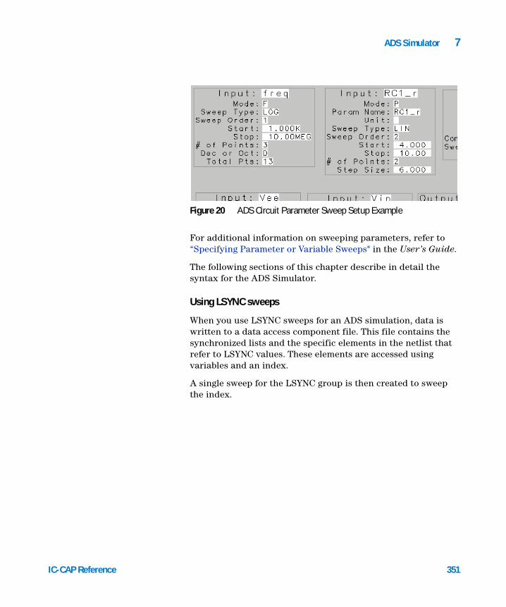
ADS Simulator 7
IC-CAP Reference
For additional information on sweeping parameters, refer to “Specifying Parameter or Variable Sweeps" in the User’s Guide.
The following sections of this chapter describe in detail the syntax for the ADS Simulator.
Using LSYNC sweeps
When you use LSYNC sweeps for an ADS simulation, data is written to a data access component file. This file contains the synchronized lists and the specific elements in the netlist that refer to LSYNC values. These elements are accessed using variables and an index.
A single sweep for the LSYNC group is then created to sweep the index.
Figure 20 ADS Circuit Parameter Sweep Setup Example
351

352
7 ADS Simulator
Example Netlist:Options ASCII_Rawfile=no UseNutmegFormat=yes
model nmos3 MOSFET nmos=yes \ UO = 1000 \Vto = 1.136 \Nfs = 0 \Tox = 1E-007 \Nsub = 5.31E+015 \Nss = 0 \Vmax = 1E+006 \Rs = 0 \Rd = 0 \Rsh = 0 \Cbd = 0 \Cbs = 0 \Cj = 0 \Mj = 0.5 \Cjsw = 0 \Mjsw = 0.33 \Is = 1E-014 \Pb = 0.8 \Fc = 0.5 \Xj = 9.438E-008 \Ld = 2.955E-007 \Delta = 0.9338 \
IC-CAP Reference

ADS Simulator 7
IC-CAP Reference
Theta = 0.04124 \Eta = 0 \Kappa = 0.2
nmos3:devckt n1 n2 n3 n4 L = lsync0_0 W = lsync0_1 Ad = 1e-10 As = 1e-10 Pd = 0.000104 Ps = 0.000104 ; START SOURCES V_Source:VGGROUND n2 0 Vdc=0 V_Source:VBGROUND n4 0 Vdc=0 V_Source:VDGROUND n1 0 Vdc=0.1 V_Source:VSGROUND n3 0 Vdc=0 ; END SOURCES
INDEX0=0#uselib "ckt" , "DAC"DAC:DAC0 File="c:\ictmp\IC19_lsync0" Type="dscr" InterpMode="index_lookup" iVar1=1 iVal1=INDEX0
lsync0_0=file {DAC0, "lval0"}lsync0_1 = file {DAC0, "lval1"}SweepPlan:swp1 Start=0 Stop=5 Step=0.2SweepPlan:swp2 Start=-3 Stop=0 Step=1.5 Reverse=yesSweepPlan:swp3 Start=0 Stop=2 Step=1DC:dc1 SweepPlan=swp1 SweepVar="VGGROUND.Vdc"ParamSweep:ct1 SimInstanceName="dc1" SweepPlan=swp2 SweepVar="VBGROUND.Vdc"ParamSweep:ct2 SimInstanceName="ct1" SweepPlan=swp3 SweepVar="INDEX0"
And the contents of IC19_lsync0 will be:BEGIN DSCRDATA% INDEX0 lval0 lval10 5e-05 5e-051 5e-05 5e-062 2.5e-06 5e-05
353

7 ADS Simulator
Interpreting this Chapter
354
To make this chapter more accurate and easier to update, much of the information in it is derived directly from the help facility in the ADS Simulator. The parameter information in the help facility has the following format.
Parameters: name (units) attributes description
Attributes: field 1: settable. s = settable. S = settable and required. field 2: modifiable. m = modifiable. field 3: optimizable. o = optimizable. field 4: readable. r = readable. field 5: type. b = boolean. i = integer. r = real number. c = complex number. d = device instance. s = character string.
Table 66 Model Parameter Attribute Definitions
Attribute Meaning Example
settable Can be defined in the instance or model statement. Most parameters are settable, there are a few cases where a parameter is calculated internally and could be used either in an equation or sent to the dataset via the OutVar parameter on the simulation component. The parameter must have its full address.
Gbe (Small signal Base-Emitter Conductance) in the BJT model can be sent to the dataset by setting OutVar=”MySubCkt.X1.Gbe” on the simulation component.
required Has no default value; must be set to some value, otherwise the simulator will return an error.
modifiable The parameter value can be swept in simulation.
IC-CAP Reference

ADS Simulator 7
IC-CAP Reference
optimizable The parameter value can be optimized.
readable Can be queried for value in simulation using the OutVar parameter. See settable.
boolean Valid values are 1, 0, True, and False.
integer The maximum value allowed for an integer type is 32767, values between 32767 and 2147483646 are still valid, but will be netlisted as real numbers. In some cases the value of a parameter is restricted to a certain number of legal values.
The Region parameter in the BJT model is defined as integer but the only valid values are 0, 1, 2, and 3.
real number The maximum value allowed is 1.79769313486231e308+.
complex number
The maximum value allowed for the real and imaginary parts is 1.79769313486231e308+.
device instance
The parameter value must be set to the name of one of the instances present in the circuit.
The mutual inductance component (Mutual), where the parameters Inductor1 and Inductor2 are defined by instance names of inductors present in the circuit or by a variable pointing to the instance names.Inductor1=”L1” or Inductor1=Xyzwhere Xyz=”L1”
character string
Used typically for file names. Must be in double quotes.
Filename=”MyFileName”
Table 66 Model Parameter Attribute Definitions
Attribute Meaning Example
355

356
7 ADS Simulator
There are 2 other identifiers not in flag format. One is [ ] next to a parameter name and it means that the parameter is structured as an array. The other is (repeatable) appended to the parameter description and it means that the parameter can appear more than once in the same instance. An example is OutVar.
IC-CAP Reference

ADS Simulator 7
General Syntax
IC-CAP Reference
In this chapter, the following typographical conventions apply:
Table 67 Typographic Conventions
Type Style Used For
[. . .] Data or character fields enclosed in brackets are optional.
italics Names and values in italics must be supplied
bold Words in bold are ADS simulator keywords and are also required.
357

7 ADS Simulator
The ADS Simulator Syntax
358
The following sections outline the basic language rules.
Field Separators
A delimiter is one or more blanks or tabs.
Continuation Characters
A statement may be continued on the next line by ending the current line with a backslash and continuing on the next line.
Name Fields
A name may have any number of letters or digits in it but must not contain any delimiters or non alphanumeric characters. The name must begin with a letter or an underscore ( _ ).
Table 68 Fundamental Units
Dimension Fundamental Unit
Frequency Hertz
Resistance Ohms
Conductance Siemens
Capacitance Farads
Inductance Henries
Length meters
Time seconds
Voltage Volts
Current Amperes
Power Watts
Distance meters
Temperature Celsius
IC-CAP Reference

ADS Simulator 7
Parameter Fields
IC-CAP Reference
A parameter field takes the form name = value, where name is a parameter keyword and value is either a numeric expression, the name of a device instance, the name of a model or a character string surrounded by double quotes. Some parameters can be indexed, in which case the name is followed by [i], [i,j], or [i,j,k]. i, j, and k must be integer constants or variables.
Node Names
A node name may have any number of letters or digits in it but must not contain any delimiters or non alphanumeric characters. If a node name begins with a digit, then it must consist only of digits.
Lower/Upper Case
The ADS Simulator is case sensitive.
Units and Scale Factors
An integer or floating point number may be scaled by following it with either an e or E and an integer exponent (e.g., 2.65e3, 1e-14).
An ADS Simulator parameter with a given dimension assumes its value has the corresponding units. For example, for a resistance, R=10 is assumed to be 10 Ohms. The fundamental units for the ADS Simulator are shown in Table 68.
A number or expression can be scaled by following it with a scale factor. A scale factor is a single word that begins with a letter or an underscore. The remaining characters, if any, consist of letters, digits, and underscores. Note that ‘‘/’’ cannot be used to represent ‘‘per’’. The value of a scale factor is resolved using the following rule: If the scale factor exactly matches one of the predefined scale-factors (Table 69), then use the numerical equivalent; otherwise, if the first character of the scale factor is one of the legal scale-factor prefixes (Table 70), the corresponding scaling is applied.
359

360
7 ADS Simulator
Predefined Scale Factors
This type of scale factor is a predefined sequence of characters which the ADS Simulator parses as a single token. The predefined scale factors are listed in the previous table.
Table 69 Predefined Scale Factors
Scale Factor Scaling Meaning
A 1 Amperes
F 1 Farads
ft 0.3048 feet
H 1 Henries
Hz 1 Hertz
in 0.0254 inches
meter 1 meters
meters 1 meters
metre 1 meters
metres 1 meters
mi 1609.344 miles
mil 2.54*10-5 mils
mils 2.54*10-5 mils
nmi 1852 nautical miles
Ohm 1 Ohms
Ohms 1 Ohms
S 1 Siemens
sec 1 seconds
V 1 Volts
W 1 Watts
IC-CAP Reference

ADS Simulator 7
IC-CAP Reference
Single-character prefixes
If the first character of the scale factor is one of the legal scale-factor prefixes, the corresponding scaling is applied.The single-character prefixes are based on the metric system of scaling prefixes and are listed in the following table
For example, 3.5 GHz is equivalent to 3.5*109 and 12 nF is equivalent to 1.2*10-8. Note that most of the time, the ADS Simulator ignores any characters that follow the single-character prefix. The exceptions are noted in “Unrecognized Scale Factors” on page 362.
Most of these scale factors can be used without any additional characters (e.g., 3.5 G, 12n). This means that m, when used alone, stands for ‘‘milli’’.
The underscore _ is provided to turn off scaling. For example, 1e-9 _farad is equivalent to 10-9, and 1e-9 farad is equivalent to 10-24.
Predefined scale factors are case sensitive.
Unless otherwise noted, additional characters can be appended to a predefined scale factor prefix without affecting its scaling value.
Table 70 Single-character prefixes
Prefix Scaling Meaning
T 1012 tera
G 109 giga
M 106 mega
K 103 kilo
k 103 kilo
- 1
m 10-3 milli
u 10-6 micro
n 10-9 nano
361

362
7 ADS Simulator
A predefined scale factor overrides any corresponding single-character-prefix scale factor. For example, 3 mm is equivalent to 3*10-3, not 3*106. In particular, note that M does not stand for milli, m does not stand for mega, and F does not stand for femto.
There are no scale factors for dBm, dBW, or temperature, see section on “Functions” on page 374 for conversion functions.
Unrecognized Scale Factors
The ADS Simulator treats unrecognizable scale factors as equal to 1 and generates a warning message.
Scale-Factor Binding
More than one scale factor may appear in an expression, so expressions like x in + y mil are valid and behave properly.
Scale factors bind tightly to the preceding variable. For instance, 6 + 9 MHz is equal to 9000006. Use parentheses to extend the scope of a scale factor (e.g., (6 + 9) MHz).
p 10-12 pico
f 10-15 femto
a 10-18 atto
Table 70 Single-character prefixes (continued)
Prefix Scaling Meaning
Booleans
Many devices, models, and analyses have parameters that are boolean valued. Zero is used to represent false or no, whereas any number besides zero represents true or yes. The keywords yes and no can also be used.
IC-CAP Reference

ADS Simulator 7
Ground Nodes
IC-CAP Reference
Node 0 is assumed to be the ground node. Additional ground node aliases can be defined using the ground statement. Multiple ground statements can be used to define any number of ground aliases, but they must all occur at the top-level hierarchy in the netlist.
General Form:
Ground [ :name ] node1 [... nodeN]
Example:Ground gnd
Global Nodes
Global nodes are user-defined nodes which exist throughout the hierarchy. The global nodes must be defined on the first lines in the netlist. They must be defined before they are used.
General Form:
globalnode nodename1 [ nodename2 ] [... nodenameN ]
Example:globalnode sumnode my_internal_node
Comments
Comments are introduced into an ADS Simulator file with a semicolon; they terminate at the end of the line. Any text on a line that follows a semicolon is ignored. Also, all blank lines are ignored.
Statement Order
Models can appear anywhere in the netlist. They do not have to be defined before a model instance is defined.
363

364
7 ADS Simulator
Some parameters expect a device instance name as the parameter value. In these cases, the device instance must already have been defined before it is referenced. If not, the device instance name can be entered as a quoted string using double quotes (").
Naming Conventions
The full name for an instance parameter is of the form:
[pathName].instanceName.parameterName[index]
where pathName is a hierarchical name of the form
[pathName].subcircuitInstanceName
The same naming convention is used to reference nodes, variables, expressions, functions, device terminals, and device ports.
For device terminals, the terminal name can be either the terminal name given in the device description, or tn where n is the terminal number (the first terminal in the description is terminal 1, etc.). Device ports are referenced by using the name pm, where m is the port number (the first pair of terminals in the device description is port 1, etc.).
Note that t1 and p1 both correspond to the current flowing into the first terminal of a device, and that t2 corresponds to the current flowing into the second terminal. If terminals 1 and 2 define a port, then the current specified by t2 is equal and opposite to the current specified by t1 and p1.
Currents
The only currents that can be accessed for simulation, optimization, or output purposes are the state currents.
State currents
Most devices are voltage controlled, that is, their terminal currents can be calculated given their terminal voltages. Circuits that contain only voltage-controlled devices can be solved using node analysis. Some devices, however, such as
IC-CAP Reference

ADS Simulator 7
IC-CAP Reference
voltage sources, are not voltage controlled. Since the only unknowns in node analysis are the node voltages, circuits that contain non-voltage-controlled devices cannot be solved using node analysis. Instead, modified node analysis is used. In modified node analysis, the unknown vector is enlarged. It contains not only the node voltages but the branch currents of the non-voltage-controlled devices as well. The branch currents that appear in the vector of unknowns are called state currents. Since the ADS Simulator uses modified node analysis, the values of the state currents are available for output.
If the value of a particular current is desired but the current is not a state current, insert a short in series with the desired terminal. The short does not affect the behavior of the circuit but does create a state current corresponding to the desired current.
To reference a state current, use the device instance name followed by either a terminal or port name. If the terminal or port name is not specified, the state current defaults to the first state current of the specified device. Note that this does not correspond to the current through the first port of the device whenever the current through the first port is not a state current. For some applications, the positive state current must be referenced, so a terminal name of t1 or t3 is acceptable but not t2. Using port names avoids this problem. The convention for current polarity is that positive current flows into the positive terminal.
365

7 ADS Simulator
Instance Statements
366
General Form:
type [ :name ] node1 ... nodeN [ [ param=value ] ... ]
type [ :name ] [ [ param=value] ... ]
Examples:ua741:OpAmp in out outC:C1 2 3 C=10pfHB:Distortion1 Freq=10GHz
The instance statement is used to define to the ADS Simulator the information unique to a particular instance of a device or an analysis. The instance statement consists of the instance type descriptor and an optional name preceded by a colon. If it is a device instance with terminals, the nodes to which the terminals of the instance are connected come next. Then the parameter fields for the instance are defined. The parameters can be in any order. The nodes, though, must appear in the same order as in the device or subcircuit definition.
The type field may contain either the ADS Simulator instance type name, or a user-supplied model or subcircuit name. The name can be any valid name, which means it must begin with a letter, can contain any number of letters and digits, must not contain any delimiters or non alphanumeric characters, and must not conflict with other names including node names.
IC-CAP Reference

ADS Simulator 7
Model Statements
IC-CAP Reference
General Form:
model name type [ [ param = value ] ... ]
Examples:model NPNbjt bjt NPN=yes Bf=100 Js=0.1fa
Often characteristics of a particular type of element are common to a large number of instances. For example, the saturation current of a diode is a function of the process used to construct the diode and also of the area of the diode. Rather than describing the process on each diode instantiation, that description is done once in a model statement and many diode instances refer to it. The area, which may be different for each device, is included on each instance statement. Though it is possible to have several model statements for a particular type of device, each instance may only reference at most one model. Not all device types support model statements.
The name in the model statement becomes the type in the instance statement. The type field is the ADS Simulator-defined model name. Any parameter value not supplied will be set to the model’s default value.
Most models, such as the diode or bjt models, can be instantiated with an instance statement. There are exceptions. For instance, the Substrate model cannot be instantiated. Its name, though, can be used as a parameter value for the Subst parameter of certain transmission line devices.
367

7 ADS Simulator
Subcircuit Definitions
368
General Form:define subcircuitName ( node1 ... nodeN )
[ parameters name1 = [ value1 ] ... name n = [ value n ] ] ...
elementStatements...
end [ subcircuitName ]
Examples:define DoubleTuner (top bottom left right)parameters vel=0.95 r=1.0 l1=.25 l2=.25 tline:tuner1 top bottom left left len=l1 vel=vel r=r tline:tuner2 top bottom right right len=l2 vel=2*vel r=rend DoubleTunerDoubleTuner:InputTuner t1 b2 3 4 l1=0.5
A subcircuit is a named collection of instances connected in a particular way that can be instantiated as a group any number of times by subcircuit calls. The subcircuit call is in effect and form, an instance statement. Subcircuit definitions are simply circuit macros that can be expanded anywhere in the circuit any number of times. When an instance in the input file refers to a subcircuit definition, the instances specified within the subcircuit are inserted into the circuit. Subcircuits may be nested. Thus a subcircuit definition may contain other subcircuits. However, a subcircuit definition cannot contain another subcircuit definition. All the definitions must occur at the top level.
An instance statement that instantiates a subcircuit definition is referred to as a subcircuit call. The node names (or numbers) specified in the subcircuit call are substituted, in order, for the node names given in the subcircuit definition. All instances that refer to a subcircuit definition must have the same number of nodes as are specified in the subcircuit definition and in the same order. Node names inside the subcircuit definition are strictly local unless they are a global ground defined with a ground statement or global nodes defined with a globalnode statement. A subcircuit definition with no nodes must still include the parentheses ( ).
IC-CAP Reference

ADS Simulator 7
IC-CAP Reference
Parameter specification in subcircuit definitions is optional. Any parameters that are specified are referred to by name followed by an equals sign and then an optional default value. If, when making a subcircuit call in your input file, you do not specify a particular parameter, then this default value is used in that instance. Subcircuit parameters can be used in expressions within the subcircuit just as any other variable.
Subcircuits are a flexible and powerful way of developing and maintaining hierarchical circuits. Parameters can be used to modify one instance of a subcircuit from another. Names within a subcircuit can be assigned without worrying about conflicting with the same name in another subcircuit definition. The full name for a node or instance include its path name in addition to its instance name. For example, if the above subcircuit is included in subckt2 which is itself included in subckt1, then the full path name of the length of the first transmission line is subckt1.subckt2.tuner1.len.
Only enough of the path name has to be specified to unambiguously identify the parameter. For example, an analysis inside subckt1 can reference the length by subckt2.tuner1.len since the name search starts from the current level in the hierarchy. If a reference to a name cannot be resolved in the local level of hierarchy, then the parent is searched for the name, and so on until the top level is searched. In this way, a sibling can either inherit its parent’s attributes or define its own.
369

7 ADS Simulator
Expression Capability
370
The ADS Simulator has a powerful and flexible symbolic expression capability, called VarEqn, which allows the user to define variables, expressions, and functions in the netlist. These can then be used to define other VarEqn expressions and functions, to specify device parameters and optimization goals, etc.
The names for VarEqn variables, expressions, and functions follow the same hierarchy rules that instance and node names do. Thus, local variables in a subcircuit definition can assume values that differ from one instance of the subcircuit to the next.
Functions and expressions can be defined either globally or locally anywhere in the hierarchy. All variables are local by default. Local variables are known in the subcircuit in which they are defined, and all lower subcircuits; they are not known at higher levels. Expressions defined at the root (the top level) are known everywhere within the circuit. To specify an expression to be global the global keyword must precede the expression. The global keyword causes the variable to be defined at the root of the hierarchy tree regardless of the lexical location.
Examples:global exp1 = 2.718
The expression capability includes the standard math operations of + - / * ^ in addition to parenthesis grouping. Scale factors are also allowed in general expressions and have higher precedence than any of the math operators (see “Units and Scale Factors” on page 359).
Constants
An integer constant is represented by a sequence of digits optionally preceded by a negative sign (e.g, 14, -3).
A real number contains a decimal point and/or an exponential suffix using the e notation (e.g, 14.0, -13e-10).
IC-CAP Reference

ADS Simulator 7
IC-CAP Reference
The only complex constant is the predefined constant j which is equal to the square root of -1. It can be used to generate complex constants from real and integer constants (e.g., j*3, 9.1 + j*1.2e-2). The predefined functions complex() and polar() can also be used to enter complex constants into an expression.
A string constant is delimited by single quotes (e.g.,’string’,’this is a string’).
Predefined Constants
Table 71 Predefined Constants
Constant Definition Constant Definition
boltzmann Boltzmann’s constant ln10 2.30...
c0 Speed of light in a vacuum
j Square root of -1
DF_DefaultInt Reference to default int value defined in Data Flow controller
pi 3.14...
DF_ZERO_OHMS Symbol for use as zero ohms
planck Planck’s constant
e 2.718... qelectron Charge of an electron
e0 Permittivity of a vacuum
tinyReal Smallest real number
hugeReal Largest real number u0 Permeability of a vacuum
Variables
General Form:
variableName = constantExpression
Examples:x1 = 4.3inches + 3milssyc_a = cos(1.0+sin(pi*3))Zin = 7.8k - j*3.2k
371

372
7 ADS Simulator
The type of a variable is determined by the type of its value. For example, x=1 is an integer, x=1+j is complex, and x = “tuesday” is a string.
Predefined Variables
In addition to the predefined constants, there are several predefined global variables. Since they are variables, they can be modified and swept.
__fdd Flag to indicate a new FDD instance
__fdd_v Flag to indicate updated FDD state vars
_ac_state Is analyses in AC state
_c1 to _c30 Symbolic controlling current
_dc_state Is analyses in DC state
_freq1 to _freq12 Fundamental frequency
_harm Harmonic number index for sources and FDD
_hb_state Is analyses in harmonic balance state
_p2dInputPower Port input power for P2D simulation
_sigproc_state Is analyses in signal processing state
_sm_state Is analyses in sm state
_sp_state Is analyses in sparameter analysis state
_tr_state Is analyses in transient state
CostIndex Index for optimization cost plots
DF_Value Reference to corresponding value defined in Data Flow controller
DefaultValue Signal processing default parameter value
DeviceIndex Device Index used for noise contribution or DC OP output
dcSourceLevel used for DC source-level sweeping
doeindex Index for Design of Experiment sweeps
freq The frequency in Hertz of the present simulation
(1MHz)
logNodesetScale Used for DC nodeset simulation
logRshunt Used for DC Rshunt sweeping
IC-CAP Reference

ADS Simulator 7
IC-CAP Reference
The sourcelevel variable is used by the spectral analysis when it needs to gradually increase source power from 0 to full scale to obtain convergence. It can be used by the user to sweep the level of ALL spectral source components, but is not recommended. The _v and _i variables should only be used in the context of the sdd device.mcTrial Trial counter for Monte Carlo based simulations
noisefreq The spectral noise analysis frequency
Nsample Signal processing analysis sample number
optIter Optimization job iteration counter
temp The ambient temperature, in degrees Celsius. (25 degrees)
time The analysis time
timestep The analysis time step
tranorder The transient analysis integration order
ScheduleCycle Signal processing schedule cycle number
sourcelevel The relative attenuation of the spectral sources (1.0)
ssfreq The small-signal mixer analysis frequency
_v1 to _v19 State variable voltages used by the sdd device
_i1 to _i19 State variable currents used by the sdd device
mc_index Index variable used by Monte Carlo controller
Expressions
General Form:
expressionName = nonconstantExpression
Examples:x1 = 4.3 + freq;syc_a = cos(1.0+sin(pi*3 + 2.0*x1))Zin = 7.8 ohm + j*freq * 1.9 phy = if (x equals 0) then 1.0e100 else 1/x endif
The main difference between expressions and variables is that a variable can be directly swept and modified by an analysis but an expression cannot. Note however, that any instance
373

374
7 ADS Simulator
parameter that depends on an expression is updated whenever one of the variables that the expression depends upon is changed (e.g., by a sweep).
Predefined Expressions
gaussian = _gaussian_tol(10.0) default gaussian distribution
nfmin = _nfmin() the minimum noise figure
omega = 2.0*pi*freq the analysis frequency
rn = _rn() the noise resistance
sopt = _sopt the optimum noise match
tempkelvin = temp + 273.15 the analysis temperature
uniform = _uniform_tol(10.0) default uniform distribution
Functions
General Form:
functionName( [ arg1, ..., argn ] ) = expression
Examples:y_srl(freq, r, l) = 1.0/(r + j*freq*l)expl(a,b) = exp(a)*step(b-a) + exp(b)*(a-b-1)*step(a-b)
In expression, the function’s arguments can be used, as can any other VarEqn variables, expressions, or functions.
Predefined Functions
_discrete_density(...) user-defined discrete density function
_gaussian( [mean, sigma, lower_n_sigmas, upper_n_sigmas, lower_n_sigmas_del,upper_n_sigmas_del] )
gaussian density function
IC-CAP Reference

ADS Simulator 7
IC-CAP Reference
_gaussian_tol[percent_tol,lower_n_sigmas, upper_n_sigmas, lower_percent_tol, upper_percent_tol, lower_n_sigmas_del,upper_n_sigmas_del] )
gaussian density function (tolerance version)
_get_fnom_freq(...) Get analysis frequency for FDD carrier frequency index and harmonic
_lfsr(x, y, z) linear feedback shift register (trigger, seed, taps)
_mvgaussian(...) multivariate gaussian density function (correlation version)
_mvgaussian_cov(...) multivariate gaussian density function (covariance version)
_n_state(x, y) _n_state(arr, val) array index nearest value
_pwl_density(...) user-defined piecewise-linear density function
_pwl_distribution(...) user-defined piecewise-linear distribution function
_randvar(distribution, mcindex, [nominal, tol_percent, x_min, x_max, lower_tol, upper_tol, delta_tol, tol_factor] )
random variable function
_shift_reg(x, y, z, t) (trigger, mode(ParIn:MSB1st), length, input)
_uniform( [lower_bound, upper_bound] )
uniform density function
_uniform_tol([percent_tol,lower_tol, upper_tol] )
uniform density function (tolerance version)
abs(x) absolute value function
access_all_data(...) datafile indep+dep lookup/interpolation function
access_data(...) datafile dependents’ lookup/interpolation function
arcsinh(x) arcsinh function
arctan(x) arctan function
atan2(y, x) arctangent function (2 real arguments)
awg_dia(x) wire gauge to diameter in meters
bin(x) function convert a binary to integer
375

376
7 ADS Simulator
bitseq(time, [clockfreq, trise, tfall, vlow, vhigh, bitseq] )
bitsequence function
complex(x, y) real-to-complex conversion function
conj(x) complex-conjugate function
cos(x) cosine function
cos_pulse(time, [low, high, delay, rise, fall, width, period] )
periodic cosine shaped pulse function
cosh(x) hyperbolic cosine function
cot(x) cotangent function
coth(x) hyperbolic cotangent function
ctof(x) convert Celsius to Fahrenheit
ctok(x) convert Celsius to Kelvin
cxform(x, y, z) transform complex data
damped_sin(time, [offset, amplitude, freq, delay, damping, phase] )
damped sin function
db(x) decibel function
dbm(x, y) convert voltage and impedance into dbm
dbmtoa(x, y) convert dbm and impedance into short circuit current
dbmtov(x, y) convert dbm and impedance into open circuit voltage
dbmtow(x) convert dBm to Watts
dbpolar(x, y) (dB,angle)-to-rectangular conversion function
dbwtow(x) convert dBW to Watts
deembed(x) deembedding function
deg(x) radian-to-degree conversion function
dep_data(x, y, [z] ) dependent variable value
dphase(x, y) Continuous phase difference (radians) between x and y
dsexpr(x, y) Evaluate a dataset expression to an hpvar
dstoarray(x, [y] ) Convert an hpvar to an array
echo(x) echo-arguments function
IC-CAP Reference

ADS Simulator 7
IC-CAP Reference
erf_pulse(time, [low, high, delay, rise, fall, width, period] )
periodic error function shaped pulse function
eval_poly(x, y, z) polynomial evaluation function
exp(x) exponential function
exp_pulse(time, [low, high, delay1, tau1, delay2, tau2] )
exponential pulse function
fread(x) raw-file reading function
ftoc(x) convert Fahrenheit to Celsius
ftok(x) convert Fahrenheit to Kelvin
get_array_size(x) Get the size of the array
get_attribute(...) value of attribute of a set of data
get_block(x, y) HPvar tree from block name function
get_fund_freq(x) Get the frequency associated with a specified fundamental index
get_max_points(x, y) maximum points of independent variable
imag(x) imaginary-part function
index(x, y, [z, t] ) get index of name in array
innerprod(...) inner-product function
int(x) convert-to-integer function
itob(x, [y] ) convert integer to binary
jn(x, y) bessel function
ktoc(x) convert Kelvin to Celsius
ktof(x) convert Kelvin to Fahrenheit
length(x) returns number of elements in array
limit_warn( [x, y, z, t, u] ) limit, default and warn function
list(...)
ln(x) natural log function
log(x) log base 10 function
mag(x) magnitude function
makearray(...) (1:real-2:complex-3:string, y, z..) or (array, startIndex, stopIndex)
max(x, y) maximum function
377

378
7 ADS Simulator
min(x, y) minimum function
multi_freq(time,amplitude, freq1, freq2, n, [seed] )
multifrequency function
names(x, y) array of names of indepVars and/or depVars in dataset
norm(x) norm function
phase(x) phase (in degrees) function
phase_noise_pwl(...) piecewise-linear function for computing phase noise
phasedeg(x) phase (in degrees) function
phaserad(x) phase (in radians) function
polar(x, y) polar-to-rectangular conversion function
polarcpx(...) polar to rectangular conversion function
pulse(time, [low, high, delay, rise, fall, width, period] )
periodic pulse function
pwl(...) piecewise-linear function
pwlr(...) piecewise-linear-repeated function
rad(x) degree-to-radian conversion function
ramp(x) ramp function
read_data(...) read_data("file-dataset", "locName", "fileType")
read_lib(...) read_lib("libName", "item", "fileType")
real(x) real-part function
rect(x, y, z) rectangular pulse function
rem(...) remainder function
ripple(x, y, z, v) ripple(amplitude, intercept, period, variable) sinusoidal ripple function
rms(...) root-mean-square function
rpsmooth(x) rectangular-to-polar smoothing function
scalearray(x, y) scalar times a vector (array) function
setDT(x) Turns on discrete time transient mode (returns argument)
IC-CAP Reference

ADS Simulator 7
IC-CAP Reference
sffm(time, [offset, amplitude, carrier_freq, mod_index,signal_freq] )
signal frequency FM
sgn(x) signum function
sin(x) sine function
sinc(x) sin(x)/x function
sinh(x) hyperbolic sine function
sprintf(x, y) formatted print utility
sqrt(x) square root function
step(x) step function
tan(x) tangent function
tanh(x) hyperbolic tangent function
vswrpolar(x, y) (VSWR,angle)-to-rectangular conversion function
NOTE The VarEqn trigonometric functions always expect the argument to be specified in radians. If the user wants to specify the angle in degrees then the VarEqn function deg() can be used to convert radians to degrees or the VarEqn function rad() can be used to convert degrees to radians.
Detailed Descriptions of the Predefined Functions
_discrete_density (x1, p1, x2, p2, …) allows the user to define a discrete density distribution: returns x1 with probability p1, x2 with probability p2, etc. The xn, pn pairs needn’t be sorted. The pns will be normalized automatically.
_gaussian( [mean, sigma, lower_n_sigmas, upper_n_sigmas, lower_n_sigmas_del, upper_n_sigmas_del] ) returns a value randomly distributed according to the standard bell-shaped curve. mean defaults to 0. sigma defaults to 1. lower_n_sigmas, upper_n_sigmas define truncation limits (default to 3). lower_n_sigmas_del and upper_n_sigmas_del define a range in which the probability is zero (a bimodal distribution). _gaussian_tol( [percent_tol, lower_n_sigmas, upper_n_sigmas, lower_percent_tol, upper_percent_tol, lower_n_sigmas_del, upper_n_sigmas_del]
379
380
7 ADS Simulator
) is similar, but percent_tol defines the percentage tolerance about the nominal value (which comes from the RANDVAR expression).
_get_fnom_freq(x) returns the actual analysis frequency associated with the carrier frequency specified in the surrounding FDD context. If x is negative, it is the carrier frequency index. If x is positive, it is the harmonic index.
_mvgaussian(N, mean1, … meanN, sigma1, … sigmaN, correlation1,2, …, correlation1,N, …, correlationN-1,N) multivariate gaussian density function (correlation version). Returns an N dimensional vector. The correlation coefficient matrix must be positive definite. _mvgaussian_cov(N, mean1, … meanN, sigma1, … sigmaN, covariance1,2, ..., covariance1,N, ..., covarianceN-1,N) is similar, but defined in terms of covariance. The covariance matrix must be positive definite.
_pwl_density(x1, p1, x2, p2, …) returns a value randomly distributed according to the piecewise-linear density function with values pn at xn, i.e. it will return xn with probability pn and return
The xn, pn pairs needn’t be sorted. The pns will be normalized automatically. _pwl_distribution(x1, p1, x2, p2, …) is similar, but is defined in terms of the distribution values. It will return a value less than or equal to xn with probability pn. The xn, pn pairs will be sorted in increasing xn order. After sorting, the pns should never decrease. The pns will be normalized so that pN=1.
_randvar(distribution, mcindex, [nominal, tol_percent, x_min, x_max, lower_tol, upper_tol, delta_tol, tol_factor] ) returns a value randomly distributed according to the distribution. The value will be the same for a given value of mcindex. The other parameters are interpreted according to the distribution.
xn ε with probability pn εpn 1+ pn–
xn 1+ xn–---------------------------++
IC-CAP Reference
ADS Simulator 7
IC-CAP Reference
_shift_reg(x, y, z, t) implements a z-bit shift register. x specifies the trigger. y = 0 means LSB First, Serial To Parallel, 1 means MSB First, Serial To Parallel, 2 means LSB First, Parallel to Serial, 3 means MSB First, Parallel to Serial. t is the input (output) value.
_uniform( [lower_bound, upper_bound] ) returns a value between lower_bound and upper_bound. All such values are equally probable. _uniform_tol( [percent_tol, lower_tol, upper_tol] ) is similar, but tolerance version.
access_all_data(InterpMode, source, indep1, dep1 …) datafile independent and dependent lookup/interpolation function.
access_data(InterpMode, nData, source, dep1 …) datafile dependents’ lookup/interpolation function.
bin(String) calculates the integer value of a sequence of 1’s and 0’s. For example bin(’11001100’) = 204. The argument of the bin function must be a string denoted by single quotes. The main use of the bin function is with the System Model Library to define an integer which corresponds to a digital word.
cxform(x, OutFormat, InFormat) transform complex data x from format InFormat to format OutFormat. The values for OutFormat and InFormat are 0: real and imaginary, 1: magnitude (linear) and phase (degrees), 2: magnitude (linear) and phase (radians), 3: magnitude (dB) and phase (degrees), 4: magnitude (dB) and phase (radians), 5: magnitude (SWR) and phase (degrees), 6: magnitude (SWR) and phase (radians). For example, to convert linear magnitude and phase in degrees to real and imaginary parts:result = cxform(invar, 0, 1)
damped_sin(time, [offset, amplitude, freq, delay, damping, phase]). See “Transient Source Functions” on page 386.
The function db(x) is a shorthand form for the expression: 20log(mag(x)).
The deembed(x) function takes an array, x, of 4 complex numbers (the 2-port S-parameter array returned from the VarEqn interp() function) and returns an array of equivalent
381

382
7 ADS Simulator
de-embedding S-parameters for that network. The array must be of length 4 (2 x 2--two-port data only), or an error message will result. The transformation used is:
where det is the determinant of the 2 x 2 array.
S111– S11
det---------=
S211– S21
det---------=
S121– S12
det---------=
S221– S22
det---------=
CAUTION This transformation assumes that the S-parameters are derived from equal port termination impedances. This transformation does not work when the port impedances are unequal.
The function deg(x) converts from radians to degrees.
dphase(x, y) Calculates phase difference phase(x)-phase(y) (in radians).
dsexpr(x, y) Evaluate x, a DDS expression, to an hpvar. y is the default location data directory.
echo(x) prints argument on terminal and returns it as a value.
erf_pulse(time, [low, high, delay, rise, fall, width, period] ) periodic pulse function, edges are error function (integral of Gaussian) shaped.
IC-CAP Reference

ADS Simulator 7
IC-CAP Reference
eval_poly(x, y, z) y is a real number. z is an integer that describes what to evaluate: -1 means the integral of the polynomial, 0 means the polynomial itself, +1 means the derivative of the polynomial. x is a VarEqn array that contains real numbers. The polynomial is
exp_pulse(time, [low, high, delay1, tau1, delay2, tau2]) See “Transient Source Functions” on page 386.
get_fund_freq(fund) returns the value of frequency (in Hertz) of a given fundamental defined by fund.
index(nameArray, "varName", [caseSense, length] ) returns position of "varName" in nameArray, -1 if not found. caseSense sets case-sensitivity, defaults to yes. length sets how many characters to check, defaults to 0 (all).
innerprod(x, y) forms the inner product of the vectors x and y:
j and k are optional integers which specify a range of harmonics to include in the calculation:
j defaults to 0 and k defaults to infinity.
int(x) Truncates the fractional part of x.
itob(x, [bits] ) convert integer x to bits-bit binary string.
The function jn(n, x) is the n-th order bessel function evaluated at x.
limit_warn( [Value, Min, Max, default, Name] ) sets Value to default, if not set. Limits it to Min and Max and generates a warning if the value is limited.
x0 x1y x2y2 x3y3…+ + +
innerprod x y,( ) xi∗ yi
i 0=
n
∑=
innerprod x y j k, , ,( ) xi∗ yi
i j=
k
∑=
383

384
7 ADS Simulator
makearray(arg1[,arg2,..] creates an array with elements defined by arg1 to argN where N can be any number of arguments. The data type of args must be Integer, Real, or Complex and the same for all args.word = bin(’1101’)fibo = makearray(0,1,1,2,3,5,8,word)foo = fibo[0]
multi_freq(time, amplitude, freq1, freq2, n, [seed] ) seed defaults to 1. If it is 0, phase is set to 0, otherwise it is used as a seed for a randomly-generated phase.
norm(x) returns the L-2 norm of the spectrum x:
j and k are optional integers which specify a range of harmonics to include in the calculation:
j defaults to 0 and k defaults to infinity.
phase(x) is the same as phasedeg(x).
The function phasedeg(x) returns phase in degrees.
The function phaserad(x) returns phase in radians.
The function polarcpx(x[,leave_as_real]) takes a complex argument, assumes that the real and complex part of the argument represents mag and phase (in radians) information, and converts it to real/imaginary. If the argument is real or integer instead of complex, the imaginary part is assumed to be zero. However, if the optional leave_as_real variable is specified, and is the value ‘‘1’’ (note that the legal values are ‘‘0’’ and ‘‘1’’ only), a real argument will be not be converted to a complex one.
pulse(time, [low, high, delay, rise, fall, width, period]) See “Transient Source Functions” on page 386.
pwl(...) piecewise-linear function. See “Transient Source Functions” on page 386.
pwlr(...) piecewise-linear-repeated function.
norm x( ) innerprod x x,( )=
norm x j k, ,( ) innerprod x x j k, , ,( )=
IC-CAP Reference

ADS Simulator 7
IC-CAP Reference
The function rect(t, tc, tp) is pulse function of variable t centered at time tc with duration tp.
The function rad(x) converts from degrees to radians.
ramp(x) 0 for , x for
read_data(source, locName, [fileType]) returns data from a file or dataset. source = “file” --- “dataset”. locName is the name of the source. fileType specifies the file type.
read_lib(libName, locName, [fileType]) returns data from a library. libName is the name of the library. locName is the name of the source. fileType specifies the file type. read_lib("libName", "item", "fileType")
rect(x, y, z) Returns:
rem(x, [y]) Returns remainder of dividing x/y. y defaults to 0 (which returns x).
rms(x) returns the RMS value (including DC) of the spectrum x:
j and k are optional integers which specify a range of harmonics to include in the calculation:
j defaults to 0 and k defaults to infinity.
The function rpsmooth(x) takes a VarEqn pointer (one returned by readraw()), converts to polar format the rectangular data given by the VarEqn pointer, and smooths out ‘phase discontinuities’.
z |x - y| < |z| |x - y| > |z|
> 0 1 0
< 0 0 1
x 0< x 0≥
rms x( ) norm x( )2.0
---------------------=
rms x j k, ,( ) norm x j k, ,( )2.0
-------------------------------=
385

7 ADS Simulator
CAUTION This function uses an algorithm that assumes that the first point is correct (i.e., not off by some multiple of ) and that the change in phase between any 2 adjacent points is less than . This interpolation will not work well with noisy data or with data within roundoff error of zero. It should be used only with S-parameters in preparation for interpolation or extrapolation by one of the interpolation functions like interp1(). Also note that the result is left in a polar ‘mag/phase’ format stored in a complex number; the real part is magnitude, and the imaginary part is phase. The polarcpx() function must be used to convert the result of the rpsmooth() function back into a real/imaginary format.
2ππ
386
sffm(time, [offset, amplitude, carrier_freq, mod_index, signal_freq]) See “Transient Source Functions” on page 386.
The sprintf() function is similar to the C function which takes a format string for argument s and a print argument x (x must be a string, an integer, or a real number) and returns a formatted string. This string then may be written to the console using the system function with an echo command.
Transient Source Functions
There are several built-in functions that mimic Spice transient sources. They are:
There functions are typically used with the vt parameter of the voltage source and the it parameter of the current source.
SPICE source ADS Simulator function
exponential exp_pulse(time, low, high, tdelay1, tau1, tdelay2, tau2)
single-frequency FM sffm(time, offset, amplitude, carrier_freq, mod_index, signal_freq)
damped sine damped_sin(time, offset, amplitude, freq, delay, damping)
pulse pulse(time, low, high, delay, rise, fall, width, period)
piecewise linear pwl(time, t1, x1, ..., tn, xn)
IC-CAP Reference

ADS Simulator 7
IC-CAP Reference
exp_pulse
Examples:ivs:vin n1 0 vt=exp_pulse(time)ics:iin n1 0 it=exp_pulse(time, -0.5mA, 0.5mA, 10ns, 5ns,20ns, 8ns)
TSTEP is the output step-time time specified on the TRAN analysis.
sffm
Examples:ivs:vin n1 0 vt=sffm(time, , , , 0.5)ics:iin n1 0 it=sffm(time, 0, 2, 1GHz, 1.2, 99MHz)
TSTOP is the stop time specified on the TRAN analysis.
Arguments for exp_pulse
Name Optional Default
TIME NO
LOW YES 0
HIGH YES 1
TDELAY1 YES 0
TAU1 YES TSTEP
TDELAY2 YES TDELAY1 + TSTEP
TAU2 YES TSTEP
Arguments for sffm
Name Optional Default
TIME NO
OFFSET YES 0
AMPLITUDE YES 1
CARRIER_FREQ YES 1/TSTOP
MOD_INDEX YES 0
SIGNAL_FREQ YES 1/TSTOP
387

388
7 ADS Simulator
damped_sin
Examples:ivs:vin n1 0 vt=damped_sin(time)ics:iin n1 0 it=damped_sin(time, 0, 5V, 500MHz, 50ns, 200ns)
TSTOP is the stop time specified on the TRAN analysis.
pulse
Examples:ivs:vin n1 0 vt=pulse(time)ics:iin n1 0 it=pulse(time, -5V, 5V, 500MHz, 50ns, 200ns)
TSTEP is the output step-time time specified on the TRAN analysis. TSTOP is the stop time specified on the TRAN analysis.
Arguments for damped_sin
Name Optional Default
TIME NO
OFFSET YES 0
AMPLITUDE YES 1
FREQ YES 1/TSTOP
DELAY YES 0
DAMPING YES 1/TSTOP
Arguments for pulse
Name Optional Default
TIME NO
LOW YES 0
HIGH YES 1
DELAY YES 0
RISE YES TSTEP
FALL YES TSTEP
WIDTH YES TSTOP
PERIOD YES TSTOP
IC-CAP Reference
ADS Simulator 7
IC-CAP Reference
pwl
Examples:ivs:vin n1 0 vt=pulse(time, 0, 0, 1ns, 1, 10ns, 1, 15ns, 0)ics:iin n1 0 it=pwl(time, 0, 0, 1ns, 1, 5ns, 1, 5ns, 0.5,10ns,0.5, 15ns, 0)
Arguments for pwl
Name Optional Default
TIME NO
T1 NO
X1 NO
T2 YES NONE
X2 YES NONE
.
.
.
.
.
.
.
.
.
TN YES NONE
XN YES NONE
Conditional Expressions
The ADS Simulator supports simple in-line conditional expressions:if boolExpr then expr else expr endifif boolExpr then expr elseif boolExpr then expr else exprendif
boolExpr is a boolean expression, that is, an expression that evaluates to TRUE or FALSE.
expr is any non-boolean expression.
The else is required (because the conditional expression must always evaluate to some value).
There can be any number of occurrences of elseif expr then expr.
A conditional expression can legally occur as the right-hand side of an expression or function definition or, if parenthesized, anywhere in an expression that a variable can occur.
389

390
7 ADS Simulator
Boolean operators
Boolean expressions
A boolean expression must evaluate to TRUE or FALSE and, therefore, must contain a relational operator (equals, =, ==, notequals, !=, <, >, <=, or >=).
The only legal place for a boolean expression is directly after an if or an elseif.
A boolean expression cannot stand alone, that is,x = a > b
is illegal.
Precedence
Tightest binding: equals, =, ==, notequals, !=, >, <, >=, <=
NOT, !
equals logical equals
= logical equals
== logical equals
notequals logical not equals
!= logical not equals
not logical negative
! logical negative
and logical and
&& logical and
or logical or
|| logical or
< less than
> greater than
<= less than or equals
>= greater than or equals
IC-CAP Reference
ADS Simulator 7
IC-CAP Reference
AND,
Loosest binding: OR, ||
All arithmetic operators have tighter binding than the boolean operators.
Evaluation
Boolean expressions are short-circuit evaluated. For example, if when evaluating a and b, expression a evaluates to FALSE, expression b will not be evaluated.
During evaluation of boolean expressions with arithmetic operands, the operand with the lower type is promoted to the type of the other operand. For example, in 3 equals x +j*b, 3 is promoted to complex.
A complex number cannot be used with <, >, <=, or >=. Nor can an array (and remember that strings are arrays). This will cause an evaluation-time error.
Pointers can be compared only with pointers.
Examples:
Protect against divide by zero:f(a) = if a equals 0 then 1.0e100 else 1.0/a endif
Nested if’s #1:f(mode) = if mode equals 0 then 1-a else f2(mode) endiff2(mode) = if mode equals 1 then log(1-a) else f3(mode) endiff3(mode) = if mode equals 2 then exp(1-a) else 0.0 endif
Nested if’s #2:f(mode) = if mode equals 0 then 1-a elseif mode equals 1 then \log(1-a) elseif mode equals 2 then exp(1-a) else 0.0 endif
Soft exponential:exp_max = 1.0e16x_max = ln(exp_max)exp_soft(x) = if x<x_max then exp(x) else
(x+1-x_max)*exp_max endif
391

7 ADS Simulator
VarEqn Data Types
392
The 4 basic data types that VarEqn supports are integer, real, complex, and string. There is a fifth data type, pointer, that is also supported. Pointers are not allowed in an algebraic expression, except as an argument to a function that is expecting a pointer. Strings are not allowed in algebraic expressions either except that addition of strings is equivalent to catenation of the strings. String catenation is not commutative, and since VarEqn’s simplification routines can internally change the order of operands of commutative operators, this feature should be used cautiously. It will most likely be replaced by an explicit catenation function.
Type conversion
The data type of a VarEqn expression is determined at the time the expression is evaluated and depends on the data types of the terms in the expression. For example, let y=3*x^2. If x is an integer, then y is integer-valued. If x is real, then y is real-valued. If x is complex, then y is complex-valued.
As another example, let y=sqrt(2.5*x). If x is a positive integer, then y evaluates to a real number. If, however, x is a negative integer, then y evaluates to a complex number.
There are some special cases of type conversion:
• If either operand of a division is integer-valued, it is promoted to a real before the division occurs. Thus, 2/3 evaluates to 0.6666....
• The built-in trigonometric, hyperbolic, and logarithmic functions never return an integer, only a real or complex number.
IC-CAP Reference

ADS Simulator 7
“C-Preprocessor”
IC-CAP Reference
Before being interpreted by the ADS Simulator, all input files are run through a built-in preprocessor based upon a C preprocessor. This brings several useful features to the ADS Simulator, such as the ability to define macro constants and functions, to include the contents of another file, and to conditionally remove statements from the input. All C preprocessor statements begin with # as the first character.
Unfortunately, for reasons of backward compatibility, there is no way to specify include directories. The standard C preprocessor “-I” option is not supported; instead, “-I” is used to specify a file for inclusion into the netlist.
File Inclusion
Any source line of the form#include "filename"
is replaced by the contents of the file filename. The file must be specified with an absolute path or must reside in either the current working directory or in /$HPEESOF_DIR/circuit/components/.
Library Inclusion
The C preprocessor automatically includes a library file if the -N command line option is not specified and if such a file exists. The first file found in the following list is included as the library:$HPEESOF_DIR/circuit/components/gemlib$EESOF_DIR/circuit/components/gemlib$GEMLIB.gemlib~/.gemlib~/gemini/gemlib
A library file is specified by the user using the -Ifilename command line option. More than 1 library may be specified. Specifying a library file prevents the ADS Simulator from including any of the above library files.
393

7 ADS Simulator
Macro Definitions
394
A macro definition has the form;#define name replacement-text
It defines a macro substitution of the simplest kind--subsequent occurrences of the token name are replaced by replacement-text. The name consists of alphanumeric characters and underscores, but must not begin with a numeric character; the replacement text is arbitrary. Normally the replacement text is the rest of the line, but a long definition may be continued by placing a “\” at the end of each line to be continued. Substitutions do not occur within quoted strings. Names may be undefined with#undef name
It is also possible to define macros with parameters. For example,#define to_celcius(t) (((t)-32)/1.8)
is a macro with the formal parameter t that is replaced with the corresponding actual parameters when invoked. Thus the lineoptions temp=to_celcius(77)
is replaced by the lineoptions temp=(((77)-32)/1.8)
Macro functions may have more than 1 parameter, but the number of formal and actual parameters must match.
Macros may also be defined using the -D command line option.
Conditional Inclusion
It is possible to conditionally discard portions of the source file. The #if line evaluates a constant integer expression, and if the expression is non-zero, subsequent lines are retained until an #else or #endif line is found. If an #else line is found, any lines between it and the corresponding #endif are discarded. If the expression evaluates to zero, lines between the #if and #else are discarded, while those between the #else and #endif are retained. The conditional inclusion statements nest to an arbitrary level of hierarchy. The following operators and functions can be used in the constant expression;
IC-CAP Reference

ADS Simulator 7
IC-CAP Reference
The #ifdef and #ifndef lines are specialized forms of #if that test whether a name is defined.
! Logical negation.
|| Logical or.
&& Logical and.
== Equal to.
!= Not equal to.
> Greater than.
< Less than.
>= Greater than or equal to.
<= Less than or equal to.
+ Addition.
defined(x) 1 if x defined, 0 otherwise.
CAUTION Execution of preprocessor instructions depend on the order in which they appear on the netlist. When using preprocessor statements make sure that they are in the proper order. For example, if an #ifdef statement is used to conditionally include part of a netlist, the corresponding #define statement is contained in a separate file and #include is used to include the content of the file into the netlist, the #include statement will have to appear before the #ifdef statement for the expression to evaluate correctly.395

7 ADS Simulator
Data Access Component
396
The Data Access Component provides a clean, unified way to access tabular data from within a simulation. The data may reside in either a text file of a supported, documented format (e.g. discrete MDIF, model MDIF, Touchstone, CITIfile), or a dataset. It provides a variety of access methods, including lookup by index/value, as well as linear, cubic spline and cubic interpolation modes, with support for derivatives.
The Data Access Component provides a "handle" with which one may access data from either a text file or dataset for use in a simulation. The DAC is implemented as a cktlib subcircuit fragment with internally known expressions names (e.g. _DAC, _TREE) that are assigned via VarEqn calls such as read_data() and access_all_data(). The accessed data can be used by other components (including models, devices, variables, subcircuit calls and other DAC instances) in the netlist, either by the specific file syntax or via the VarEqn function dep_data().
The DAC can also be used to supply parameters to device and model components from text files and datasets. In this case, the AllParams device/model parameter is used to refer to a DAC component. The component’s parameters will then be accessed from the DAC and supplied to the instance. Care is taken to ensure that only matching (between parameter names in the component definition and DAC dependent column names) data is used. Also, parameter data can be assigned "inline" - as is usually done - in which case the inline data takes precedence over the DAC data.
As the DAC component is composed of just a parameterized subcircuit, it allows alterations (sweep, tune, optimize, yield) of its parameters. Consequently any component that uses DAC data via file, dep_data() or AllParams will automatically be updated when a DAC parameter is altered. A caveat with sweeping over files using AllParams is that all the files must contain the same number of dependent columns of data.
Below is an example definition of a simple DAC component that accesses discrete values from a text file:
IC-CAP Reference

ADS Simulator 7
IC-CAP Reference
#uselib "ckt" , "DAC"DAC:DAC1 File="C:\jeffm\ADS_testing\ADS13_test_prj/.\data\SweptData.ds"Type="dataset" Block="S" InterpMode="linear" InterpDom="ri"iVar1="X" iVal1=X iVar2="freq" iVal2=freqS_Port:S2P1 _net1 0 _net6 0 S[1,1]=file{DAC1, "S[1,1]"}S[1,2]=file{DAC1,"S[1,2]"} S[2,1]=1 S[2,2]=0 Recip=no
dindex = 1DAC:atc1 File="vdcr.mdf" Type="dscr" \ InterpMode="index_lookup" iVar1=1 iVal1=dindex
And its use to provide the resistance value to a pair of circuit components:R:R1 n1 0 R=file{atc1, "R"} kOhmR:R2 n1 0 R=dep_data(atc1, "R") kOhmHere, it provides the value to a variable:V1 = file{atc1, "Vdc"}
V1 could be used elsewhere in the circuit, as expected.
In this example, a scaling factor applied to the result of a DAC access is shown:File = "atc.mdf"Type = "dscr"Mode="index_lookup"Cnom = "Cnom" DAC:atc_s File=File Type=Type InterpMode=Mode iVar1=1 iVal1 = Cs_rowC:Cs n1 n2 C=file{atc_s, Cnom} Pf
In this example, a use of AllParams is shown to enter model parameters from a text file:File = "c:\gemini\vdcr.mdf"Type = "dscr"Mode="index_lookup"DAC:dac1 File=File Type=Type InterpMode=Mode iVar1=1 iVal1 = ixmodel rm1 R_Model R=0 AllParams = dac1._DACrm1:rm1i1 n3 0
397

7 ADS Simulator
Reserved Words
398
The words on the following pages have built-in meaning and should not be defined or used in a way not consistent with their pre-defined meaning:
AC CPWCPL4
ACPWDS CPWCTL
ACPWDTL CPWDS
AIRIND1 CPWEF
Alter CPWEGAP
Amplifier CPWG
AmplifierP2D CPWOC
AntLoad CPWSC
BFINL CPWSUB
BFINLT CPWTL
BJT CPWTLFG
BR3CTL CTL
BR4CTL C_Model
BRCTL Chain
BROCTL Chebyshev
Bessel Connector
BudLinearization CostIndex
Butterworth Crossover
C DC
CAPP2 DF
CAPQ DFDevice1
CIND2 DFDevice2
CLIN DF_DefaultInt
CLINP DF_Value
COAX DF_ZERO_OHMS
COAXTL DICAP
CPW DILABMLC
IC-CAP Reference
ADS Simulator 7
IC-CAP Reference
CPWCGAP DOE
CPWCPL2 DRC
DefaultValue JFET
DeviceIndex L
Diode LineCalcTest
EE_BJT2 MACLIN
EE_FET3 MACLIN3
EE_HEMT1 MBEND
EE_MOS1 MBEND2
ETAPER MBEND3
Elliptic MBSTUB
FDD MCFIL
FINLINE MCLIN
FSUB MCORN
GCPWTL MCROS
GMSK_Lowpass MCROSO
GaAs MCURVE
Gaussian MCUREVE2
Goal MGAP
HB MICAP1
HP_Diode MICAP2
HP_FET MICAP3
HP_FET2 MICAP4
HP_MOSFET MLANG
Hybrid MLANG6
IFINL MLANG8
IFINLT MLEF
INDQ MLIN
I_Source MLOC
InitCond MLSC
InoiseBD MLYRSUB
MOS9 MSRTL
MOSFET MSSLIT
399
400
7 ADS Simulator
MRIND MSSPLC
MRINDELA MSSPLR
MRINDELM MSSPLS
MRINDNBR MSSTEP
MRINDSBR MSSVIA
MRINDWNR MSTAPER
MRSTUB MSTEE
MS2CTL MSTEP
MS3CTL MSTL
MS4CTL MSUB
MS5CTL MSVIA
MSABND MSWRAP
MSACTL MTAPER
MSAGAP MTEE
MSBEND MTEEO
MSCRNR MTFC
MSCROSS MextramBJT
MSCTL Mixer
MSGAP MixerIMT
MSIDC Multipath
MSIDCF Mutual
MSLANGE NodeSet
MSLIT NoiseCorr2Port
MSOBND Noisey2Port
MSOC Nsample
MSOP OldMonteCarlo
MSRBND OldOpt
OldOptim PC_Corner
OldYield PC_CrossJunction
Optim PC_Crossover
OptimGoal PC_Gap
Options PC_Line
OscPort PC_OpenStub
IC-CAP Reference

ADS Simulator 7
IC-CAP Reference
OutSelector PC_Pad
PCBEND PC_Slanted
PCCORN PC_Taper
PCCROS PC_Tee
PCCURVE PC_Via
PCILC PIN
PCLIN1 PIN2
PCLIN10 PLCQ
PCLIN2 ParamSweep
PCLIN3 PinDiode
PCLIN4 PoleZero
PCLIN5 Polynomial
PCLIN6 Port
PCLIN7 PowerBounce
PCLIN8 PowerGroundPlane
PCLIN9 R
PCSTEP RCLIN
PCSUB RIBBON
PCTAPER RIBBON_MDS
PCTEE RIND
PCTRACE RWG
PC_Bend RWGINDF
PC_Clear RWGT
RWGTL SLSTEP
R_Model SLTEE
RaisedCos SLTL
SAGELIN SLUCTL
SAGEPAC SLUTL
SBCLIN SMITER
SBEND SOCLIN
SBEND2 SPIND
SCLIN SS3CTL
SCROS SS4CTL
401

402
7 ADS Simulator
SCURVE SS5CTL
SDD SSACTL
SL3CTL SSCLIN
SL4CTL SSCTL
SL5CTL SSLANGE
SLABND SSLIN
SLCQ SSSPLC
SLCRNR SSSPLR
SLCTL SSSPLS
SLEF SSSUB
SLGAP SSTEP
SLIN SSTFR
SLINO SSTL
SLOBND SSUB
SLOC SSUBO
SLOC_MDS STEE
SLOTTL S_Param
SLRBND S_Port
SLSC ScheduleCycle
Short VBIC
Substrate VIA
SweepPlan VIA2
SwitchV V_Source
SwitchV_Model VnoiseBD
TAPIND1 WIRE
TFC WIRE_MDS
TFC_MDS Y_Port
TFR Yield
TFR_MDS YieldOptim
TL YieldSpec
TLIN YieldSpecOld
TLIN4 Z_Port
TLINP __fdd
IC-CAP Reference

ADS Simulator 7
IC-CAP Reference
TLINP4 __fdd_v
TL_New _ac_state
TQAVIA _c1
TQCAP _c10
TQFET _c11
TQFET2 _c12
TQIND _c13
TQRES _c14
TQSVIA _c15
TQSWH _c16
TQTL _c17
Tran _c18
UFINL _c19
UFINLT _c2
Unalter _c20
_c21 _freq6
_c22 _freq7
_c23 _freq8
_c24 _freq9
_c25 _gaussian
_c26 _gaussian_tol
_c27 _get_fnom_freq
_c28 _get_fund_freq_for_fdd
_c29 _harm
_c3 _hb_state
_c30 _i1
_c4 _i10
_c5 _i11
_c6 _i12
_c7 _i13
_c8 _i14
_c9 _i15
_dc_state _i16
403

404
7 ADS Simulator
_default _i17
_discrete_density _i18
_divn _i19
_freq1 _i2
_freq10 _i20
_freq11 _i21
_freq12 _i22
_freq2 _i23
_freq3 _i24
_freq4 _i25
_freq5 _i26
_i27 _sopt
_i28 _sp_state
_i29 _sv
_i3 _sv_bb
_i30 _sv_d
_i4 _sv_e
_i5 _tn
_i6 _to
_i7 _tr_state
_i8 _tt
_i9 _uniform
_lfsr _uniform_tol
_mvgaussian _v1
_mvgaussian_cov _v10
_n_state _v11
_nfmin _v12
_p2dInputPower _v13
_phase_freq _v14
_pwl_density _v15
_pwl_distribution _v16
_randvar _v17
_rn _v18
IC-CAP Reference

ADS Simulator 7
IC-CAP Reference
_shift_reg _v19
_si _v2
_si_bb _v20
_si_d _v21
_si_e _v22
_sigproc_state _v23
_sm_state _v24
_v25 conj
_v26 cos
_v27 cos_pulse
_v28 cosh
_v29 cot
_v3 coth
_v30 coupling
_v4 ctof
_v5 ctok
_v6 cxform
_v7 d_atan2
_v8 damped_sin
_v9 db
_xcross dbm
abs dbmtoa
access_all_data dbmtov
access_data dbmtow
aele dbpolar
and dbwtow
arcsinh dcSourceLevel
arctan deembed
atan2 define
awg_dia deg
bin delay
bitseq dep_data
boltzmann deriv
405

406
7 ADS Simulator
by discrete
c0 distcompname
complex doe
doeindex generate_qam16_spectra
dphase generate_qpsk_pulse_spectra
dsexpr get_array_size
dstoarray get_attribute
e get_block
e0 get_fund_freq
echo get_max_points
else global
elseif globalnode
end ground
endif hugereal
equals i
erf_pulse if
eval_poly ilsb
exp imag
exp_pulse index
file innerprod
fread inoise
freq int
freq_mult_coef internal_generate_gmsk_iq_spectra
freq_mult_poly internal_generate_gmsk_pulse_spectra
ftoc internal_generate_piqpsk_spectra
ftok internal_generate_pulse_train_spectra
gauss internal_generate_qam16_spectra
gaussian internal_generate_qpsk_pulse_spectra
generate_gmsk_iq_spectra internal_get_fund_freq
generate_gmsk_pulse_spectra internal_window
generate_piqpsk_spectra interp
generate_pulse_train_spectra interp1
interp2 names
IC-CAP Reference

ADS Simulator 7
IC-CAP Reference
interp3 nested
interp4 nf
iss nfmin
itob no
iusb nodoe
jn noisefreq
ktoc noopt
ktof norm
lbtran nostat
length not
limit_warn notequals
list omega
ln opt
ln10 optIter
local or
log parameters
logNodesetScale phase
logRshunt phase_noise_pwl
log_amp phasedeg
log_amp_cas phaserad
mag planck
makearray polar
max polarcpx
mcTrial ppt
mcindex pulse
min pwl
model pwlr
multi_freq qelectron
qinterp sprintf
rad sqrt
ramp ssfreq
randtime stat
rawtoarray step
407
408
7 ADS Simulator
read_data strcat
read_lib stypexform
readdata sym_set
readlib system
readraw tan
real tanh
rect temp
rem tempkelvin
ripple thd
rms then
rn time
rpsmooth timestep
scalearray tinyreal
sens to
setDT toi
sffm tranorder
sgn transform
sin u0
sinc unconst
sine unicap
sinh uniform
sink v
sopt value
sourceLevel vlsb
vnoise
vss
vswrpolar
vusb
window
yes
IC-CAP Reference

Agilent 85190A IC-CAP 2008Reference
8IC-CAP Functions
This chapter describes the IC-CAP functions. They appear in alphabetical order.
When reviewing the functions, keep in mind the following points:
• Many functions can be called from within a Program or Macro. Several examples are provided here; additional examples can be found in “Calls to the Function Library” on page 752.
• The list does not represent all the functions available in a Program or Macro. Additional built-in functions are available in the Parameter Extraction Language. Refer to “Built-in Functions” on page 714.
• For consistency, the argument names listed for each function reflect the descriptive labels these arguments would get in a standalone Transform editor.
• The Input Arguments referred to as Strings/Pars/Vars can be any of the following alternatives: string expressions, Model parameter names, DUT parameter names, or IC-CAP system variable names.
The tables that follow list the available functions by category, as they appear in the program.
409Agilent Technologies

410
8 IC-CAP Functions
Table 72 IC-CAP FunctionsAHBT
AgilentHBT_ABCX_extract AgilentHBT_calculate_ccb AgilentHBT_calculate_rbb
AgilentHBT_CCMAX_extract AgilentHBT_CEMAX_extract AgilentHBT_CJC_extract
AgilentHBT_CJE_extract AgilentHBT_IS_NF_extract AgilentHBT_ISC_NC_extract
AgilentHBT_ISE_NE_extract AgilentHBT_ISH_NH_extract AgilentHBT_ISR_NR_extract
AgilentHBT_ISRH_NRH_extract AgilentHBT_ITC_ITC2_extract AgilentHBT_Param_Init
AgilentHBT_TFC0_extract AgilentHBT_VJC_extract AgilentHBT_VJE_extract
ATFT (obsolete)
HPTFTCV_model_cgd HPTFTDC_lin HPTFTDC_sat
HPTFTCV_model_cgs HPTFTDC_model_id HPTFT_param
B2200
B2200_bias_card_enable B2200_bias_ch_enable B2200_bias_enable
B2200_bias_init B2200_close_interface B2200_connect
B2200_couple_enable B2200_couple_setup B2200_debug
B2200_disconnect_card B2200_GPIB_handler B2200_ground_card_enable
B2200_ground_enable B2200_ground_init B2200_ground _outch_enable
B2200_ground _unused_inputs B2200_init B2200_open_interface
BJT
BJTAC_high_freq BJTDC_rc BJTCV_stoc
BJTAC_rb_rbm_irb BJTDC_rcfb RBBcalc
BJTDC_fwd_gummel BJTDC_re H11corr
BJTDC_is_nf BJTDC_rev_gummel BJT_dc_model
BJTDC_nr BJTDC_vaf_var HFBJT_linear_ssmod_sim
HFBJT_linear_elem_extr
BPOPAMP
BPOPAMP_macro_model
BSIM1 (obsolete)
BSIM1DC_geom_indep BSIM1DC_sub BSIMCV_total_cap
BSIM1DC_lin_sat
BSIM2 (obsolete)
BSIM2DC_geom_indep BSIM2_save_dev_pars BSIM2_lin_plot
BSIM2DC_lin_sat BSIMCV_total_cap
IC-CAP Reference

IC-CAP Functions 8
BSIM3
BSIM3_set_opt BSIM3DC_sat_narrow BSIM3DC_vth
BSIM3DC_bulk_short BSIM3DC_sat_short BSIM3DC_vth_sim
BSIM3DC_lin_large BSIM3DC_sat_short2 BSIM3DC_vth_versus
BSIM3DC_lin_narrow BSIM3DC_sub_short BSIM3CVmodCBD
BSIM3DC_lin_short BSIM3DC_sub_short2 BSIM3CVmodCBS
BSIM3DC_lin_small BSIM3DC_model BSIM3CV_total_cap
BSIM3_calculate BSIM3_toolkit_vth BSIM3_check_par
BSIM3_DC_vth BSIM3_DC_calculate BSIM3_DC_get_parameter
BSIM3_DC_calc_bin_parameter BSIM3_error
BSIM4
BSIM4_check_par BSIM4_DC_get_parameter BSIM4_error
BSIM4_DC_calculate BSIM4_DC_extr_A0_AGS_KETA BSIM4_set_opt
BSIM430_DC_calculate BSIM4_DC_vth
BSIM450_DC_calculate BSIM430_DC_vth
BSIM4_DC_calc_bin_parameter BSIM450_DC_vth
Data Exchange
ICMSarray ICMSpin SPECSSpin
ICMSchar ICMSreal LINKarray
ICMSint ICMSstr LINKchar
LINKint LINKpin LINKreal
LINKstr
Data Export
icdb_add_comment icdb_close icdb_export_data
icdb_get_sweep_value icdb_open icdb_register_con_sweep
icdb_register_lin_sweep icdb_register_list_sweep icdbf_add_comment
icdbf_close icdbf_export_data icdbf_get_sweep_value
icdbf_open icdbf_register_con_sweep icdbf_register_lin_sweep
icdbf_register_list_sweep icdb_register_lsync_sweep icdbf_register_lsync_sweep
Data Fit
autofit circlefit linfit
fit_line
Table 72 IC-CAP Functions (continued)
IC-CAP Reference 411

8 IC-CAP Functions
Diode
DIODEDCmod_ia
EEBJT
EEbjt2_Is_N EEbjt2_ce_dc_iv EEbjt2_ce_ss_elements
EEbjt2_extrinsic_ckt EEbjt2_mdl HFMOD_get_bias_size
HFMOD_get_freq_index HFMOD_get_freq_value HFMOD_remove_freq_dbl
HFMOD_remove_freq_mat
EEFET
EEfet3_ckt EEfet3_model_name EEfet3_Rs_delta_s
EEfet3_cs_dc_iv EEfet3_package EEfet3_s2ckt
EEfet3_lecp EEfet3_ResCheck EEfet3_spars
EEfet3_mdl EEfet3_Rs_delta_m
EEMOS (obsolete)
EEmos1_ckt EEmos1_mdl EEmos1_ResCheck
EEmos1_cs_dc_iv EEmos1_model_name EEmos1_s2ckt
EEmos1_lecp EEmos1_package EEmos1_spars
Flicker Noise
NOISE_1f_bjt_1Hz NOISE_1f_bjt_calc NOISE_1f_bjt_extract
NOISE_1f_force_bias NOISE_1f_get_Af NOISE_1f_get_Bf
NOISE_1f_get_Ef NOISE_1f_get_Kf NOISE_1f_mos_1Hz
NOISE_1f_set_Af NOISE_1f_set_Bf NOISE_1f_set_Ef
NOISE_1f_set_Kf NOISE_1f_stop_bias
GAAS
GAASAC_cur GAASDC_lev1 GAASmod_cgd
GAASAC_l_and_r GAASDC_lev2 GAASmod_cgs
GAASAC_r_and_c GAASDC_rd GAASmod_id
GAASCV_cgs_cgd GAASDC_rs GAASmod_ig
GAASDC_cur1 GAASAC_calc_rc GAASAC_calc_rl
GAASDC_cur2
General Math
RMSerror conjg log10
TwoPort correlation mean
Table 72 IC-CAP Functions (continued)
412 IC-CAP Reference

IC-CAP Functions 8
TwoPort2 cos random
abs cosh sin
acs derivative sinh
acsh derivative2 smooth3
arg equation sqrt
asn exp tan
asnh log tanh
atn floor variance
atnh integral0 mem_diag
ceil integral3
HF MOS Level3 (obsolete)
HFMOS3_capas HFMOS3_paras HFMOS3_StoC
HFMOS3_lin_large HFMOS3_sat_short HFMOS3_StoZ
HFMOS3_lin_narrow HFMOS3_sub_large HFMOS3_modcap
HFMOS3_lin_short HFMOS3_total_cap
HiSIM2
HiSIM2_DC_vth
HiSIM_HV
HiSIM_HV_DC_vth
HPIB
HPIB_abort HPIB_open HPIB_spoll
HPIB_clear HPIB_read_reals HPIB_srq
HPIB_close HPIB_readnum HPIB_timeout
HPIB_command HPIB_readstr HPIB_write
HPIB_eoi HPIB_fwrite HPIB_read
HPMOS
HPMOSDC_lin_large HPMOSDC_lin_short HPMOS_process_pars
HPMOSDC_lin_narrow HPMOSDC_sat_short
HPRoot Diode
HPdiode_C HPdiode_S11i HPdiode_para_at_f
HPdiode_C2 HPdiode_S11r HPdiode_para_f
HPdiode_I HPdiode_V HPdiode_wr
Table 72 IC-CAP Functions (continued)
IC-CAP Reference 413

8 IC-CAP Functions
HPdiode_Q HPdiode_data_acqu HPRoot_n
HPdiode_R HPdiode_mdl HPdiode_fgrt
HPdiode_fless HPdiode_iextr
HPRoot Fet
HPRoot_data_acqu HPRoot_Qd HPRoot_Y12r
HPRoot_FET HPRoot_Qg HPRoot_Y21i
HPRoot_initial HPRoot_Vd HPRoot_Y21r
HPRoot_parasitic HPRoot_Vg HPRoot_Y22i
HPRoot_Id HPRoot_Y11i HPRoot_Y22r
HPRoot_Idh HPRoot_Y11r HPRoot_FET_t
HPRoot_Ig HPRoot_Y12i HPRoot_fet_acqu
HPRoot_n HPRoot_para_cal HPRoot_wr
HPRoot Mos
HPRoot_Id HPRoot_Vd HPRoot_Y12r
HPRoot_Idh HPRoot_Vg HPRoot_Y21i
HPRoot_Ig HPRoot_Y11i HPRoot_Y21r
HPRoot_Qd HPRoot_Y11r HPRoot_Y22i
HPRoot_Qg HPRoot_Y12i HPRoot_Y22r
HPRoot_MOSFET HPRoot_mos_acqu HPRoot_mos_para
HPRoot_para_cal
JUNCAP
JUNCAP JUNCAP_TR
MEXTRAM
MXT_I0 MEXTRAM_stoc MXT_cbc
MXT_cbe MXT_cj0 MXT_csc
MXT_forward_hfe MXT_forward_ic MXT_forward_vbe
MXT_ft MXT_VEF MXT_ic_vce
MXT_VER MXT_hard_sat_isub MXT_reverse_isub
MXT_jun_cap MXT_reverse_currents MXT_reverse_hfc
MXT_reverse_hfc_sub MXT_veaf_ib MXT_veaf_ic
MXT_vear_ie MXT_show_parms
MEXTRAM 503 (obsolete)
Table 72 IC-CAP Functions (continued)
414 IC-CAP Reference

IC-CAP Functions 8
mxt_smooth mxt3t_cbc mxt3t_cbe
mxt3t_cj0 mxt3t_ft_ic mxt3t_ft_ic_new
mxt3t_fwd_early_ib mxt3t_fwd_early_ic mxt3t_fwd_gummel_hfe
mxt3t_fwd_gummel_ib mxt3t_fwd_gummel_ic mxt3t_fwd_gummel_vbe
mxt3t_i0 mxt3t_linear_range mxt3t_output_ic
mxt3t_output_vbe mxt3t_rev_early_ie mxt3t_rev_early_qb0_guess
mxt3t_rev_gummel_hfc mxt3t_rev_gummel_ib mxt3t_rev_gummel_ie
mxt4t_cbc mxt4t_cbe mxt4t_cj0
mxt4t_csc mxt4t_ft_ic mxt4t_ft_ic_new
mxt4t_fwd_early_ib mxt4t_fwd_early_ic mxt4t_fwd_gummel_hfe
mxt4t_fwd_gummel_ib mxt4t_fwd_gummel_ic mxt4t_fwd_gummel_vbe
mxt4t_i0 mxt4t_linear_range mxt4t_output_ic
mxt4t_output_vbe mxt4t_rev_early_ie mxt4t_rev_early_qb0_guess
mxt4t_rev_gummel_hfc mxt4t_rev_gummel_hfc_sub mxt4t_rev_gummel_ib
mxt4t_rev_gummel_ie mxt4t_rev_gummel_is
MM9
MM9_LIN_EXT MM9_COPY MM9_SAVE_SPARS
MM9_SAT_EXT MM9_DATA MM9_SETUP
MM9_STH_EXT MM9_GEOMPAR MM9_TEMPPAR
MM9_WEAVAL_EXT MM9_GEOMSCAL MM9_TEMPSCAL
MM9 MM9_KEEP
MOS Level1
MOSmodel MOSmodel2
MOS Level2
MOSCV_total_cap MOSDC_lev2_lin_short MOSCVmodCBS
MOSDC_lev2_lin_large MOSDC_lev2_sat_short MOSmodel
MOSDC_lev2_lin_narrow MOSCVmodCBD MOSmodel2
MOS Level3
MOSCV_total_cap MOSDC_lev3_lin_short MOSCVmodCBS
MOSDC_lev3_lin_large MOSDC_lev3_sat_short MOSmodel2
MOSDC_lev3_lin_narrow MOSCVmodCBD
MOS Level6
Table 72 IC-CAP Functions (continued)
IC-CAP Reference 415

8 IC-CAP Functions
MOSCV_total_cap MOSDC_lev6_lin_narrow MOSCVmodCBD
MOSDC_lev6_lin_large MOSDC_lev6_lin_short MOSCVmodCBS
MOS Process
MOS_process_pars
Optimization
Optimize
PEL
Program or Program2
PN Capacitance
PNCAPsimu
PSP
PSP_DC_vth PSP_check_par PSP_DC_calc_bin_parameter
PSP_set_opt
PTFT (obsolete)
PTFTCV_cgd PTFTDC_lin PTFTDC_sat
PTFTCV_cgs
Random Functions
rand_flat rand_gauss rand_seed
Statistical Analysis
icstat_get_column icstat_deactivate icstat_set_text_cell
icstat_set_column icstat_attribute_2_parameter icstat_open
icstat_num_columns icstat_parameter_2_attribute icstat_write_to_status_window
icstat_num_rows icstat_analysis icstat_exit
icstat_get_cell icstat_correlation icstat_open_sdf_file
icstat_set_cell icstat_stat_summary icstat_close_sdf_file
icstat_num_deactivated icstat_factor_analysis icstat_save_sdf_file
icstat_num_filtered icstat_parametric_models icstat_to_partable
icstat_num_attributes icstat_equations icstat_from_partable
icstat_get_deactivated icstat_plot_graph icstat_set_param_column_labels
icstat_get_filtered_rows icstat_set_row iicstat_nonparametric_models
icstat_get_attribute_columns icstat_get_row icstat_clear
icstat_activate icstat_get_text_cell icstat_delete
Table 72 IC-CAP Functions (continued)
416 IC-CAP Reference

IC-CAP Functions 8
icstat_insert
Switching Matrix
Connect SWM_debug Wait
FNPort SWM_init HP5250_bias_card
HP5250_card_config HP5250_bias_channel HP5250_bias_init
HP5250_bias_setmode HP5250_compensate_cap HP5250_connect
HP5250_couple_enable HP5250_couple_setup HP5250_debug
HP5250_disconnect_card HP5250_init HP5250_show
K707_init K708a_init K70X_clear_setup
K70X_close_crosspoints K70X_config_trigger K70X_connect_sequence
K70X_copy_setup K70X_debug K70X_delete_setup
K70X_edit_setup K70X_init_interface K70X_open_crosspoints
K70X_trigger_disable K70X_trigger_enable
Target
TARGET_DC_vth
TRL Calibration
8753_TRL_Cal TRL_Cal
USERC
USERC_init_param USERC_open USERC_sweep_start
USERC_avg_2 USERC_read_reals USERC_sweep_stepsize
USERC_avg_3 USERC_readnum USERC_sweep_stop
USERC_conjg USERC_readstr USERC_system
USERC_transpose USERC_seek USERC_tell
USERC_close USERC_set_param USERC_write
USERC_data_w_check USERC_size USERC_sweep_name
USERC_num_of_points USERC_set_param_quiet USERC_sweep_mode
USERC_get_object_name
User Defined
Holding place for user-defined functions. For details, refer to “Adding Functions to the Function Browser" in the User’s Guide.
Utility
Table 72 IC-CAP Functions (continued)
IC-CAP Reference 417

8 IC-CAP Functions
check_error_log copy2output Package
dataset lookup_par lookup_var
ascii$
VBIC
VBIC_ac_solver VBIC_avc VBIC_cbc
VBIC_cbe VBIC_cj0 VBIC_clean_data
VBIC_csc VBIC_dc_approx VBIC_dci_solver
VBIC_dcv_solver VBIC_fg_currents VBIC_ibci_nci
VBIC_ibei_nei VBIC_ikf VBIC_stoc
VBIC_ikr VBIC_is_nf VBIC_isp_nfp
VBIC_nr VBIC_qcdepl VBIC_rcx
VBIC_rg_currents VBIC_vef_ver
Wafer Prober
Pdown Porig Prober_status
Phome Ppos Pscale
Pimove Prober_debug Pup
Pink Prober_init PB_bindex
Pmove Prober_reset PB_gsite_xy
PB_abort PB_bincode PB_msite_xy
PB_bindex_cr PB_index_cr PBench_CMD
PB_index PB_gindex_cr tis_p_down
tis_p_home tis_p_imove tis_p_ink
tis_p_move tis_p_orig tis_p_pos
tis_p_scale tis_p_up tis_prober_get_ba
tis_prober_get_name tis_prober_init tis_prober_read_sysconfig
tis_prober_reset tis_prober_status
Wire Functions
wirexfX wirexfY wirexfYX
wirexfXY
Table 72 IC-CAP Functions (continued)
418 IC-CAP Reference

IC-CAP Functions 8
IC-CAP Reference
8753_TRL_Cal Deembed the raw measured data using measured data of TRL (thru-reflect-line) calibration standards. The function calculates and downloads the error coefficients to the 8753. The reference plane is defined at the middle of the thru standard, or at the interface to the DUT when it is installed in the compatible carrier.
abs Absolute value function (magnitude when input data is complex)
Inputs:
Freq Data: Frequency Inputs
Thru: measured S-parameters of the Thru standard
Short: measured S-parameters of the Short standard
Line A: measured S-parameters of Line A standard
Line B: measured S-parameters of Line B standard
Line C: measured S-parameters of Line C standard
Freq 1 Trans: transition frequency Line A to Line B
Freq 1 Trans: transition frequency Line B to Line C
Outputs: None
Input Arguments:
Data Sets: Input 1
Output: Real number, matrix, real array, or matrix array (depends on input argument)
Automatic Invocation: On Data Set Input Change
419

420
8 IC-CAP Functions
acs Inverse cosine in radians.
acsh Inverse hyperbolic cosine.
AgilentHBT_ABCX_extract This function extracts model parameter ABCX.
AgilentHBT_calculate_ccb This function calculates Cbc in an alternative method from the specified Z-parameters.
Input Arguments:
Data Sets: Input 1
Output: Complex number, matrix, complex array, or matrix array (depends on input argument)
Automatic Invocation: On Data Set Input Change
Input Arguments:
Data Sets: Input 1
Output: Complex number, matrix, complex array, or matrix array (depends on input argument)
Automatic Invocation: On Data Set Input Change
Input Arguments:
Variables: Emitter Area, Total Area
Parameters: Parameter(ABCX)
Extracts: ABCX
Input Arguments:
Inputs: freq, Z11, Z12, Z21, Z22
Output: Complex data sets.
IC-CAP Reference
IC-CAP Functions 8
IC-CAP Reference
AgilentHBT_calculate_rbb This function calculates Rb in an alternative method from the specified H-parameters.
AgilentHBT_CCMAX_extract This function extracts model parameter CCMAX.
AgilentHBT_CEMAX_extract This function extracts model parameter CEMAX.
AgilentHBT_CJC_extract This function extracts model parameter CJC.
Input Arguments:
Inputs: freq, H11, H12, H21, H22
Variables: Mode (0:ignore RE effect, 1:include RE effect)
Parameters: Parameter(RE)
Output: Complex data sets
Input Arguments:
Inputs: Vbc (as positive value), Cbc
Parameters: Parameter(CCMAX), Parameter(VJC)
Extracts: CCMAX
Input Arguments:
Inputs: Vbe, Cbe
Parameters: Parameter(CEMAX), Parameter(VJE)
Extracts: CEMAX
Input Arguments:
Inputs: Vbc (as positive value), Cbc
421

422
8 IC-CAP Functions
AgilentHBT_CJE_extract This function extracts model parameter CJE.
AgilentHBT_IS_NF_extract This function extracts model parameters IS, NF.
AgilentHBT_ISC_NC_extract This function extracts model parameters ISC, NC.
Parameters: Parameter(CJC), Parameter(CPBC)
Extracts: CJC
Input Arguments:
Inputs: Vbe, Cbe
Parameters: Parameter(CJE), Parameter(CPBE)
Extracts: CJE
Input Arguments:
Inputs: Vbe, Ic
Variables: X Low, X High, Y Low, Y High, TEMP
Parameters: Parameter(IS), Parameter(NF)
Extracts: IS, NF
Input Arguments:
Inputs: Vcb (as positive value), Ib
Variables: X Low, X High, Y Low, Y High, TEMP
Parameters: Parameter(ISC), Parameter(NC)
Extracts: ISC, NC
IC-CAP Reference
IC-CAP Functions 8
IC-CAP Reference
AgilentHBT_ISE_NE_extract This function extracts model parameters ISE, NE.
AgilentHBT_ISH_NH_extract This function extracts model parameters ISH, NH.
AgilentHBT_ISR_NR_extract This function extracts model parameters ISR, NR.
AgilentHBT_ISRH_NRH_extract This function extracts model parameters ISRH, NRH.
Input Arguments:
Inputs: Vbe, Ib
Variables: X Low, X High, Y Low, Y High, TEMP
Parameters: Parameter(ISE), Parameter(NE)
Extracts: ISE, NE
Input Arguments:
Inputs: Vbe, Ib
Variables: X Low, X High, Y Low, Y High, TEMP
Parameters: Parameter(ISH), Parameter(NH)
Extracts: ISH, NH
Input Arguments:
Inputs: Vcb (as positive value), Ie
Variables: X Low, X High, Y Low, Y High, TEMP
Parameters: Parameter(ISR), Parameter(NR)
Extracts: ISR, NR
423
424
8 IC-CAP Functions
AgilentHBT_ITC_ITC2_extract This function extracts model parameters ITC, ITC2.
AgilentHBT_Param_Init This function initializes the model parameters for the extraction.
AgilentHBT_TFC0_extract This function extracts model parameter TFC0.
Input Arguments:
Inputs: Vcb (as positive value), Ib
Variables: X Low, X High, Y Low, Y High, TEMP
Parameters: Parameter(ISRH), Parameter(NRH)
Extracts: ISRH, NRH
Input Arguments:
Inputs: Ic, Ft, Vc, Vb
Variables: X Low, X High, Y Low, Y High
Parameters: Parameter(ITC), Parameter(ITC2)
Extracts: ITC, ITC2
Input Arguments:
Variables: Emitter Width (W) [um]Emitter Length (L) [um]# of Emitter Fingers (NF)Total Area [um^2]
Parameters: Parameter(hbt.TNOM)
Extracts: All Agilent-HBT model parameters
Input Arguments:
Inputs: Ic or Ic-1, Tau, Vc, Vb
IC-CAP Reference

IC-CAP Functions 8
IC-CAP Reference
AgilentHBT_VJC_extract This function extracts model parameter VJC.
AgilentHBT_VJE_extract This function extracts model parameter VJE.
arg Argument (phase angle), in radians, for a complex number.
Variables: X Low, X High, Y Low, Y High
Parameters: Parameter(TFC0)
Extracts: TFC0
Input Arguments:
Inputs: Vbc (as positive value), Cbc, Cdiff
Parameters: Parameter(VJC), Parameter(CJC), Parameter(CPBC)
Extracts: VJC
Input Arguments:
Inputs: Vbe, Cbe, Cdiff
Parameters: Parameter(VJE), Parameter(CJE), Parameter(CPBE)
Extracts: VJE
Input Arguments:
Data Sets: Input 1
Output: Real number, matrix, real array, or matrix array (depends on input argument)
Automatic Invocation: On Data Set Input Change
425

426
8 IC-CAP Functions
ascii$ Converts ascii-coded characters into literal characters as entered into a text box.
If certain characters are entered in a text box, they must be encoded so they are compatible with the .mdl file format used in variable tables. These characters include double quotes (“) and newlines (\n). Such characters may be entered in a GUI’s edit box and tracked by a variable table variable. IC-CAP must encode these characters before storing them in a .mdl file to avoid undesirable effects.
After the characters are encoded, they appear as encoded characters if you choose to print them from the .mdl file to an output such as the Status window. To translate the encoding, call the function ascii$() in PEL and the string will be output exactly as it was typed into the text box.
asn Inverse sine in radians.
asnh Inverse hyperbolic sine.
atn Inverse tangent in radians.
Input Arguments:
Data Sets: Input 1
Output: Complex number, matrix, complex array, or matrix array (depends on input argument)
Automatic Invocation: On Data Set Input Change
Input Arguments:
Data Sets: Input 1
Output: Complex number, matrix, complex array, or matrix array (depends on input argument)
Automatic Invocation: On Data Set Input Change
IC-CAP Reference

IC-CAP Functions 8
IC-CAP Reference
atnh Inverse hyperbolic tangent.
autofit Performs an automatic line fit to a set of X and Y data sets. This function finds the largest region of the line that fits with less than the specified error from the RMS limit field. A buffer can be specified that removes a certain percentage of the data from each end of the curve. This eliminates data points that may throw off the line fit. The percentages should be specified out of 1. For example, 0.01 = 1%. If the OVERRIDE_LIMITS variable is TRUE, the limits can be specified manually with the X_LOW and X_HIGH variables, which can be set from the Plot menu.
This function should only be used on data with a single sweep variable. A 3 point data set, containing slope and intercept data and the regression coefficient, is returned.
Input Arguments:
Data Sets: Input 1
Output: Complex number, matrix, complex array, or matrix array (depends on input argument)
Automatic Invocation: On Data Set Input Change
Input Arguments:
Data Sets: Input 1
Output: Complex number, matrix, complex array, or matrix array (depends on input argument)
Automatic Invocation: On Data Set Input Change
Input Arguments:
Data Sets: X Data, Y Data
Reals or Integers: RMS limit, Buffer
427

428
8 IC-CAP Functions
Example PEL Statement:fit_data = autofit(-ve,log(ic.m),0.01,0.1)
B2200_bias_card_enable Bias-enables all the output ports of the specified card. By default, all ports are bias-enabled after a reset.
SyntaxB2200_bias_card_enable(<addr>, <CardNumber>, <CardState>)
Where
<addr> is the GPIB address of the Mainframe (must be a positive number from 1 to 30).
<CardNumber> is 0(auto), 1, 2, 3, or 4.
<CardState> is the card output port's state (allowed values are "ENABLE", "DISABLE", "E", or "D").
B2200_bias_ch_enable Bias-enables specific output ports in the channel list for the specified card. The input ports specified in the channel list are ignored since the input port is always the Bias Input Port. By default, all the outputs are bias-enabled after a reset.
SyntaxB2200_bias_ch_enable(<addr>,<CardNumber>,<State>, <Channel list>)
Where
<addr> is the GPIB address of the Mainframe (must be a positive number from 1 to 30).
<CardNumber> is 0(auto), 1, 2, 3, or 4.
<State> is the output port's state (allowed values are "ENABLE", "DISABLE", "E", or "D")
Output: Array of 2 points: slope then intercept
Automatic Invocation: None
IC-CAP Reference

IC-CAP Functions 8
IC-CAP Reference
<Channel list> is the list of channels, known as connection routes. Example channel list: (@10102, 10203, 10305:10307)
B2200_bias_enable Enables the bias mode for the specified card once Input Bias Port and Enabled Output ports are specified. When Bias Mode is ON, the Input Bias Port is connected to all Bias Enabled output ports that are not connected to any other input ports. Bias Disabled output ports are never connected to an Input Bias Port when Bias Mode is ON.
If another input port is disconnected from a bias enabled output port, this port is automatically connected to the Input Bias Port.
If another input port is connected to a Bias Enabled output port, the output port is automatically disconnected from the Bias Input Port. When Bias Mode is OFF, the Input Bias Port is the same as the other ports.
SyntaxB2200_bias_enable(<addr>, <CardNumber>, <mode>)
Where
<addr> is the GPIB address of the Mainframe (must be a positive number from 1 to 30).
<CardNumber> is 0(auto), 1, 2, 3, or 4.
<mode> is "On", "Off", "1", or "0".
B2200_bias_init Selects the Input Bias Port for the specified card. The Input Bias Port is the dedicated bias port.
SyntaxB2200_bias_init(<addr>, <CardNumber>, <InputBiasPort>)
Where
<addr> is the GPIB address of the Mainframe (must be a positive number from 1 to 30).
<CardNumber> is 0(auto), 1, 2, 3, or 4.
429

430
8 IC-CAP Functions
<InputBiasPort> is 1 to 14 (numeric input) or −1 to disable bias port.
B2200_close_interface Closes the current interface, which was opened by calling B2200_open_interface().
B2200_connect Connects or disconnects specified channels. Bias Mode and coupling Mode are also taken into account when a channel is closed or opened.
For example, in the list (@10102, 10203:10205), the following channels are connected or disconnected on card 1. Input port 1 to output port 2. Input port 2 to output port 3 and 5.
SyntaxB2200_connect(<addr>,<Connect/Disconnect>,<ChannelList>)
Where
<addr> is the GPIB address of the Mainframe (must be a positive number from 1 to 30).
<Connect/Disconnect> is C or D.
<ChannelList> is the list of connections to close.
B2200_couple_enable Enables or disables Couple Port mode. Couple Port mode allows synchronized connection of two adjacent input ports to two adjacent output ports.
SyntaxB2200_couple_enable(<addr>, <CardNumber>, <Mode>)
Where
<addr> is the GPIB address of the Mainframe (must be a positive number from 1 to 30).
<CardNumber> is 0(auto), 1, 2, 3, or 4.
<mode> is "On", "Off", "1", or "0".
B2200_couple_setup Selects the couple ports for Kelvin connections. At Reset, no input ports are coupled.
Syntax
IC-CAP Reference

IC-CAP Functions 8
IC-CAP Reference
B2200_couple_setup( <addr>,<CardNumber>, <ListOfCoupledPorts>)
Where
<addr> is the GPIB address of the Mainframe (must be a positive number from 1 to 30).
<CardNumber> is 0(auto), 1, 2, 3, or 4.
<ListOfCoupledPorts> is the list of odd number input channels (e.g., "1, 3, 5" means coupled ports are 1-2, 3-4, 5-6).
B2200_debug Prints out all command strings sent to the instrument when set to 1. This flag is common to all B2200A’s on the bus, regardless of their GPIB address.
SyntaxB2200_debug(<flag>)
Where
<flag> is "1", "0", "Yes", or "No".
B2200_disconnect_card Opens all relays or channels in the specified cards.
SyntaxB2200_disconnect_card(<addr>, <CardNumber>)
Where
<addr> is the GPIB address of the Mainframe (must be a positive number from 1 to 30).
<CardNumber> is 0(auto), 1, 2, 3, or 4.
B2200_GPIB_handler Returns -1 if the interface has not been initialized (invalid handler). Returns a positive integer (handler) if the interface has been opened.
Returns the current interface handler. The function is provided as a utility function, which enables you to write advanced PEL code to write and read data to the B2200A using the HPIB_write and HPIB_read functions. Initializing the handler using B2200_open_interface enables you to use
431

432
8 IC-CAP Functions
B2200A's built-in driver functions as well as writing PEL code to support other features that are not currently supported by the built-in functions, all in the same PEL code.
B2200_ground_card_enable Enables ground-enabling for all the output ports of the specified card. By default, all ports are ground-disabled.
SyntaxB2200_ground_card_enable(<addr>,<CardNumber>,<CardState>)
Where
<addr> is the GPIB address of the Mainframe (must be a positive number from 1 to 30).
<CardNumber> is 0(auto), 1, 2, 3, or 4.
<CardState> is the card output port's state (allowed values are "ENABLE", "DISABLE", "E", or "D").
B2200_ground_enable Enables the bias mode for the specified card. When Ground Mode is turned ON, the Input Ground Port (default is 12) is connected to all the Ground Enabled input/output ports that have not been connected to any other port. At Reset, Ground Mode is OFF. Ground Mode cannot be turned ON when Bias Mode is ON.
See the Agilent B2200 User's Guide for additional comments and restrictions.
SyntaxB2200_ground_enable(<addr>, <CardNumber>, <mode>)
Where
<addr> is the GPIB address of the Mainframe (must be a positive number from 1 to 30).
<CardNumber> is 0(auto), 1, 2, 3, 4.
<mode> is "On", "Off", "1", or "0".
IC-CAP Reference

IC-CAP Functions 8
IC-CAP Reference
B2200_ground_init Selects the input Ground Port for the specified card. For each card, you can specify the same or a different Ground Port. By default, the input Ground Port is port 12. The ground port should be connected to 0 V output voltage. See the Agilent B2200 User's Guide for details.
SyntaxB2200_ground_init(<addr>,<CardNumber>,<InputGroundPort>)
Where
<addr> is the GPIB address of the Mainframe (must be a positive number from 1 to 30).
<CardNumber> is 0(auto), 1, 2, 3, or 4.
<InputGroundPort> is 1 to 14 (numeric input) or −1 to disable ground port.
B2200_ground _outch_enable Ground-enables or ground-disables output ports. When Ground Mode is turned ON, the ground-enabled output ports that have not been connected to any other input port are connected to the input ground port. The input ports specified in channel lists are ignored since the input port is always the Input Ground Port. By default, all the outputs are ground-disabled after a reset.
SyntaxB2200_ground _outch_enable(<addr>,<CardNumber>,<State>, <Channel list>)
Where
<addr> is the GPIB address of the Mainframe (must be a positive number from 1 to 30).
<CardNumber> is 0(auto), 1, 2, 3, or 4.
<State> is the port's state (allowed values are "ENABLE", "DISABLE", "E", or "D").
<Channel list> is the list of channels, known as connection routes. Example channel list: (@10102, 10203, 10305:10307)
433

434
8 IC-CAP Functions
B2200_ground _unused_inputs Specifies the ground-enabled (or unused) input ports for the specified card. When Ground Mode is turned ON, the ground-enabled input ports that have not been connected to any other port are connected to the input Ground Port. By default, all the inputs are ground-disabled after a reset.
SyntaxB2200_ground _unused_inputs(<addr>,<CardNumber>,<Input Channels>)
Where
<addr> is the GPIB address of the Mainframe (must be a positive number from 1 to 30).
<CardNumber> is 0(auto), 1, 2, 3, 4.
<Input Channels> is the list of input channels (e.g., "1, 2, 5"). Only input ports 1 to 8 can be defined as unused (these are the input Kelvin Ports).
B2200_init Must be run first in the PEL program to initialize the instrument and set the configuration mode. When the instrument is in AUTO configuration mode and multiple plug-in cards are installed in the B2200 slots from slot 1 continuously, the installed cards are then treated as one card (numbered 0). This function resets all the settings to factory default before setting the configuration mode.
This function also sets the default connection rule for the specified card. When the connection rule is FREE (default mode), each input port can be connected to multiple output ports and each output port can be connected to multiple input ports. When the connection is SINGLE, each input port can be connected to only one output. Connection sequence specifies the open/close sequence of the relays when changing from an existing connection to a new connection.
SyntaxB2200_init( <addr>, <cardNumber>, <config>, <connectionRule>, <connectionSequence>)
Where
IC-CAP Reference

IC-CAP Functions 8
IC-CAP Reference
<addr> is the GPIB address of the Mainframe (must be a positive number from 1 to 30).
<cardNumber> is 0(auto), 1, 2, 3, or 4.
<config> is "AUTO" or "NORMAL" (string input).
<connectionRule> is "FREE" or "SINGLE".
<connectionSequence> is "NSEQ", "BBM", or "MBBR".
• NSEQ (No SEQuence): Disconnect old route, connect new route.
• BBM (Break Before Make): Disconnect old route, wait, connect new route.
• MBBR (Make Before BReak): Connect new route, wait, disconnect old route.
B2200_open_interface Opens and initializes the GPIB interface and must be run first in the PEL program. The interface handler is saved in a static variable so that the interface will be shared by all the other B2200's function calls. You can drive multiple B2200 instruments as long as they are on the same interface bus (obviously, they must have different addresses).
SyntaxB2200_open_interface(<Interface Name>)
Where
<Interface Name> is the name of the GPIB interface.
BJT_dc_model Calculates collector current (IC), base current (IB) or gain (BETA) versus terminal voltages for a bipolar transistor using the UCB DC bipolar model. Set the Output field to IC, IB, or BETA. Use this function in place of an actual simulation for fast optimizations. The source code for this function is provided as an example in the userc.c file.
Input Arguments:
Data Sets: VC, VB, VE
Strings/Pars/Vars Output
435

436
8 IC-CAP Functions
BJTAC_high_freq Standard extraction for the UCB Bipolar model. Extracts AC parameters from a common emitter measurement of H-parameters. Requires the following setup:
H versus Vbe, with Vce = 1V and 3V, and Freq constant.
The frequency value must be past the pole frequency of the device. Optimization can be used to tune the parameter values; typically, it should not be required.
BJTAC_rb_rbm_irb Standard extraction for the UCB Bipolar model. Extracts base resistance parameters from a common emitter measurement of H11. Requires the following setups:
Ib versus Vbe, with Vce = constantH11 versus Freq versus Vbe, with Vce = constant
BJTCV_stoc Calculates capacitance data from S-parameter data using the following equations:
Output: Array of real numbers; size determined by inputs
Automatic Invocation: None
Input Arguments:
Data Sets: Base Voltage, Frequency, Col Voltage, Sub Voltage, H-Par Output
Output: None
Extracts: TF, ITF, XTF, VTF, PTF
Automatic Invocation: By Extract menu function
Input Arguments:
Data Sets: IB Data, RBB Data
Output: None
Extracts: RB, RBM, IRB
Automatic Invocation: By Extract menu function
IC-CAP Reference

IC-CAP Functions 8
IC-CAP Reference
Cbc(Vbc) = − imag(Y12)/(2*pi*freq)
Cbe(Vbe) = imag(Y11)/(2*pi*freq) - Cbc(Vbc)
This allows base-collector and base-emitter capacitance to be calculated from network analyzer measurements. The output of this function can be used in place of actual capacitance data to extract capacitance related parameters.
BJTDC_fwd_gummel Standard extraction for the UCB Bipolar model. Extracts forward Gummel parameters from forward Gummel plot measurements. Requires the following setup:
Ic and Ib versus Vbe, with Vcb = 0V.
The measured data should include high and low current roll-off effects in the gain. The Vbe lower limit for extraction is automatically selected. If the OVERRIDE_LIMITS variable is true, this limit can be specified manually with the X_LOW variable, which can be set from the Plot menu. Optimization can be used to tune the parameter values, but should not typically be required.
Input Arguments:
Data Sets: FREQ data, S data
Strings/Pars/Vars: Node (C/E)
Output: Array of real numbers; size determined by inputs
Automatic Invocation: On Data Set Input Change
Input Arguments:
Data Sets: Fwd VBE, Fwd IC, Fwd IB, Fwd Beta
Output: None
Extracts: ISE, NE, BF, IKF
Automatic Invocation: By Extract menu function
437

438
8 IC-CAP Functions
BJTDC_is_nf Standard extraction for the UCB Bipolar model. Extracts saturation current parameters from forward gummel plot measurements. Requires the following setup:
Ic and Ib versus Vbe, with Vcb = 0V.
The Vbe limits for extraction are automatically selected. If the OVERRIDE_LIMITS variable is true, these limits can be specified manually with the X_LOW and X_HIGH variables, which can be set from the Plot menu. Optimization can be used to tune the parameter values, but should not typically be required.
BJTDC_nr Standard extraction for the UCB Bipolar model. Extracts NR from reverse Gummel Plot measurements. Requires the following setup:
Ie and Ib versus Vbc, with Veb = 0V.
The Vbc limits for extraction are automatically selected. If the OVERRIDE_LIMITS variable is true, these limits can be specified manually with the X_LOW and X_HIGH variables, which can be set from the Plot menu. Optimization can be used to tune the parameter value, but should not typically be required.
Input Arguments:
Data Sets: Fwd VBE, Log10 Fwd IC
Output: None
Extracts: IS, NF
Automatic Invocation: By Extract menu function
Input Arguments:
Data Sets: Rev VBC, Log10 Rev IE
Output: None
Extracts: NR
Automatic Invocation: By Extract menu function
IC-CAP Reference

IC-CAP Functions 8
IC-CAP Reference
BJTDC_rc Standard extraction for the UCB Bipolar model. Extracts collector resistance in the saturation region. Requires the following setup:
Ic versus Vce, with Vbe = typical operating value.
Depending on the device, optimization to this and other DC measurements may be required to tune the parameter value.
BJTDC_rcfb Alternate extraction for the UCB Bipolar model. Extracts collector resistance using the flyback technique. Requires the following setup:
Vec versus Ib, with the emitter floating.
Depending on the device, optimization to this and other DC measurements may be required to tune the parameter value.
BJTDC_re Standard extraction for the UCB Bipolar model. Extracts emitter resistance using the flyback technique. Requires the following setup:
Vce versus Ib, with the collector floating.
Depending on the device, optimization to this and other DC measurements may be required to tune the parameter value.
Input Arguments:
Data Sets: VC Data, IC Data
Output: None
Extracts: RC
Automatic Invocation: By Extract menu function
Input Arguments:
Data Sets: IB Data, VE Data
Output: None
Extracts: RC
Automatic Invocation: By Extract menu function
439

440
8 IC-CAP Functions
BJTDC_rev_gummel Standard extraction for the UCB Bipolar model. Extracts reverse Gummel parameters from reverse Gummel plot measurements. Requires the following setup:
Ie and Ib versus Vbc, with Veb = 0V.
The measured data should include high and low current roll-off effects in the gain. The Vbc lower limit for extraction is automatically selected. If the OVERRIDE_LIMITS variable is true, this limit can be specified manually with the X_LOW variable, which can be set from the Plot menu. Optimization can be used to tune the parameter values, but should not typically be required.
BJTDC_vaf_var Standard extraction for the UCB Bipolar model. Extracts forward and reverse early voltages from common emitter and common collector curves. Requires the following setups:
Ic versus Vce versus Vbe. Ie versus Vec versus Vbc.
The setups should have the same number of base voltage steps. The base voltages should be chosen so that current levels correspond to the peak gain regions of the device. No more than 20 percent of the data should be in the saturation
Input Arguments:
Data Sets: IB Data, VC Data
Output: None
Extracts: RE
Automatic Invocation: By Extract menu function
Input Arguments:
Data Sets: Rev VBC, Rev IE, Rev IB, Rev Beta
Output: None
Extracts: ISC, NC, BR, IKR
Automatic Invocation: By Extract menu function
IC-CAP Reference

IC-CAP Functions 8
IC-CAP Reference
region. Optimization can be used to tune the parameter values, but should not typically be required. Optimization of these parameters should be performed only after extracting the complete DC model.
BPOPAMP_macro_model Extraction function for the Boyle-Pederson- Solomon-Cohn Opamp macromodel written in C code. (Refer to IEEE JSSC vol. SC-9, no. 6, Dec. 1974.) Extracts circuit element values for a specified set of opamp performance measurements. The data set inputs to the extraction function may be from outputs of Setups that measure the specific opamp performance or from values known via other sources such as specifications on a data sheet. The real and integer inputs are not generally measurable and are taken from the knowledge of the design of the opamp being modeled. An expanded description of the inputs is given in parentheses where applicable.
Input Arguments:
Data Sets: Forward VC, Forward VB, Forward IC, Reverse VE, Reverse VB, Reverse IE
Output: None
Extracts: VAF, VAR
Automatic Invocation: By Extract menu function
Input Arguments:
Data Sets: Slew Rate +(V/uS), Slew Rate -(V/uS), Bias Current(Amps), Bias Offset(Amps), Volt Offset(Volts), Av(DM) (gain-no unit), BW(Hz), Excess Phase(radians), CMRR (dB), Rout(ohms), Rout-ac(ohms), Isc +(Amps), Isc -(Amps), Vout_max +(Volts), Vout_min -(Volts), Power Diss(Watts), Vcc supply(Volts), Vee supply(Volts)
441

442
8 IC-CAP Functions
BSIM1DC_geom_indep This function is obsolete.
Generates the BSIM geometry independent parameters (all parameters scaled to channel length and width) from a device file generated either by the BSIM extraction routines in IC-CAP or from a compatible BSIM characterization system.
Reals or Integers: Nom. Q.IS(nominal input transistor saturation current), R2(mid-stage gain setting resistor), Comp. Cap.(compensation capacitance), Temp.(C), Inputs PNP?(=1 if input stage uses pnps), Debug?(=1 print debug information during extraction)
Output: None
Extracts: NPN1.BF, NPN1.IS, NPN2.BF, NPN2.IS, C1, RC1, RC2, RE1, RE2, RE, CE, RP, GCM, GA, R2, C2, GB, RO2, RC, RO1, DMOD1.IS, DMOD2.IS, VC, VE, IEE
Automatic Invocation: By Extract menu function
Input Arguments: None
Output: None
IC-CAP Reference

IC-CAP Functions 8
IC-CAP Reference
BSIM1DC_lin_sat This function is obsolete.
Extracts the linear and saturation region parameters of the BSIM model using Id versus Vg curves for a single device.
Extracts: VFB, LVFB, WVFB, PHI, LPHI, WPHI, K1, LK1, WK1, K2, LK2, WK2, ETA, LETA, WETA, MUZ, U1, LU1, WU1, DL, DW, X2E, LX2E, WX2E, X3D, LX3E, WX3E, X2MZ, LX2MZ, WX2MZ, MUS, LMUS, WMUS, X2MS, LX2MS, WX2MS, X3MS, LX3MS, WX3MS, X2U0, LX2U0, WX2U0, X2U1, LX2U1, WX2U1, X3U1, LX3U1, WX3U1
If subthreshold parameters are extracted, the following geometry independent parameters are also extracted: N0, LN0, WN0, NB, LNB, WNB, ND, LND, WND
Automatic Invocation: By Extract menu function
Input Arguments:
Data Sets: Gate V, Bulk V, Drain V, Drain I
Output: None
Extracts: The linear region parameters: VFB, PHI, K1, K2, U0, X2U0.
The saturation region parameters: ETA, MUZ, U1, X2MZ, X2E, X3E, X2U1, MUS, X2MS, X3MS, X3U1.
Automatic Invocation: By Extract menu function
443

444
8 IC-CAP Functions
BSIM1DC_sub This function is obsolete.
Extracts the BSIM subthreshold parameters for a single device using 4 Id versus Vg curves.
BSIM2_lin_plot This function is obsolete.
Acquires specified parameter value data versus 1/W or 1/L and displays plot.
BSIM2_save_dev_pars This function is obsolete.
Appends the set of BSIM2 extracted parameters for a single device to the device file in the user’s home directory.
Input Arguments:
Data Sets: Gate V, Bulk V, Drain V, Drain I 1, Drain I 2, Drain I 3, Drain I 4
Output: None
Extracts: N0, NB, ND
Automatic Invocation: By Extract menu function
Input Arguments:
Data Sets: Input an output data set with both measured and simulated data types set
Strings/Pars/Vars: Parameter name of parameter to be plotted against 1/W or 1/L, Sort Key - W or L
Output: Array of real numbers; size determined by inputs
Automatic Invocation: None
Input Arguments: None
Output: None
Automatic Invocation: By Extract menu function
IC-CAP Reference

IC-CAP Functions 8
IC-CAP Reference
BSIM2DC_geom_indep This function is obsolete.
Generates the BSIM2 geometry independent parameters (all parameters scaled to channel length and width) from a device file generated by the BSIM2 extraction routines in IC-CAP or from a compatible BSIM2 characterization system.
Input Arguments: None
Output: None
Extracts: VFB, LVFB, WVFB, PHI, LPHI, WPHI, K1, LK1, WK1, K2, LK2, WK2, ETA0, LETA0, WETA0, MU0, DL, DW, UA0, LUA0, WUA0, U10, LU10, WU10, MU0B, LMU0B, WMU0B, ETAB, LETAB, WETAB, UB0, LUB0, WUB0, UAB, LUAB, WUAB, U1B, LU1B, WU1B, MUS0, LMUS0, WMUS0, MUSB, LMUSB, WMUSB, UBB, LUBB, WUBB, U1D, LU1D, WU1D, N0, LN0, WN0, NB, LNB, WNB, ND, LND, WND, MU20, LMU20, WMU20,MU2B, LMU2B, WMU2B, MU2G, LMU2G, WMU2G, MU30, LMU30, WMU30, MU3B, LMU3B, WMU3B, MU3G, LMU3G, WMU3G, MU40, LMU40, WMU40, MU4B, LMU4B, WMU4B, MU4G, LMU4G, WMU4G, VOF0, LVOF0, WVOF0, VOFB, LVOFB, WVOFB, VOFD, LVOFD, WVOFD, AI0, LAI0, WAI0, AIB, LAIB, WAIB, BI0, LBI0, WBI0, BIB, LBIB, WBIB, VGHIGH, LVGHIGH, WVGHIGH, VGLOW, LVGLOW, WVGLOW
Automatic Invocation: By Extract menu function
445

446
8 IC-CAP Functions
BSIM2DC_lin_sat This function is obsolete.
Extracts the linear, saturation, and subthreshold region parameters of the BSIM2 model using 2 families of Id versus Vg curves for a single device. Also extracts the output resistance parameters of the BSIM2 model using 2 families of Id versus Vd curves for a single device.
BSIM3_calculate Calculates the drain current of the BSIM3v3.2 model and different internal states of the model for the given terminal voltages vd, vg, vs, and vb. The type of internal state, for example, the drain source resistance rds can be selected by the select output flag. In some cases it is necessary to use a measured value for the threshold voltage instead of the calculated. Use the select input flag to select measured or calculated. If this is not equal to zero, then the value in value input is used for vth instead of the calculated one.
Input Arguments:
Data Sets: Gate V, Bulk V, Drain V, Drain I vs Vg, Drain I vs Vd
Output: None
Extracts: The linear region parameters: VFB, PHI, K1, K2, MU0, MU0B, UA0, UAB, UB0, UBB, VGHIGH, VGLOW.
The saturation region parameters: MUS0, MUSB, U10, U1B, ETA0, ETAB, VOF0, VOFD, VOFB.
The subthreshold region parameters: N0, NB, ND.
The output resistance parameters: MU20, MU2B, MU2G, MU30, MU3B, MU3G, MU40, MU4B, MU4G, AI0, AIB, BI0, BIB, U1D
Automatic Invocation: By Extract menu function
IC-CAP Reference

IC-CAP Functions 8
IC-CAP Reference
Input Arguments:
Variables: vd Drain voltage vg Gate voltagevs Source voltagevb Bulk voltageLength (L) Gate length Width (W) Gate widthselect input (if 1 use value input for Vth)value input (value input for Vth if select input = 1)
Parameters: None
Output: Value to calculate or failure indicatoroutput[0] = lx;output[1] = wx;output[2] = vbseff;output[3] = vt0;output[4] = nonlat;output[5] = dvtx;output[6] = dvtx_w;output[7] = k3w0;output[8] = eta_vd;output[9] = vth;output[10] = vgsteff;output[11] = abulk;output[12] = ueff;output[13] = rds;output[14] = vdsat;output[15] = vdseff;output[16] = idlin;output[17] = idr;output[18] = vasat;output[19] = vaclm;output[20] = vadiblc;output[21] = inv_vascbe;output[22] = va;output[23] = idout;
Extracts: Nothing
447

448
8 IC-CAP Functions
BSIM3_check_par Checks whether a model parameter is in a predefined range. The range information for this parameter must be given in a variable in the referenced path. The range information is stored in a string in the following format:
range_A0>-1 0 10 - | | | |___ upper error condition ({operator(<,<=), value}{-)} | | |______ upper optimization boundary| |___________ lower optimization boundary|______________ lower error condition ({operator(>,>=), value}{-)}
Example call in PEL:check = BSIM3_check_par(prwg,"PRWG",
"/BSIM3_DC_CV/Extraction_configuration/Boundaries")
BSIM3_DC_calc_bin_parameter This function calculates from the input the 4 binning parameters P0, PL, PW, and PP. If the calculation is done correctly, outputs[0] will return 0. Otherwise, outputs[0] will result in a negative number. In such a case, the error will be printed in detail in the output window.
Input Arguments:
Variables: Actual value of parameter to check
Parameters: Parameter namePath to parameter range definition
Output: Flag for correct operation:0: parameter is in specified range−1: parameter is outside specified
range−2: error during function execution (e.g., variable 'range_xx' not found)
IC-CAP Reference

IC-CAP Functions 8
IC-CAP Reference
Example call in PEL:complex l[4]complex w[4]:
l[0]= 1u:par = BSIM3_DC_get_parameter()bin_par = BSIM3_DC_calc_bin_parameter(p, l, w, par)
BSIM3_DC_calculate Calculates the drain current of the BSIM3v3.2 model and different internal states of the model for the given terminal voltages vd, vg, vs, and vb. The type of internal state, for example, the drain source resistance rds can be selected by the select output flag. In some cases, it is necessary to use a measured value for the threshold voltage instead of the calculated. Use the select input flag to select measured or calculated. If this is not equal to zero, then the value in value input is used for vth instead of the calculated one.
Input Arguments:
Inputs: Array with 4 parameters P1 .. P4 of the bin corners
Array with 4 gate lengths L1 .. L4 of the bin corners
Array with 4 gate widths W1 .. W4 of the bin corners
Array with 4 values for the numberof gate fingers NF1 .. NF4 of the bin corners
Parameter set (get with'BSIM3_DC_get_parameter()')
Output: Array containing error condition and binning parametersoutputs[0] = error condition
(0=o.k., any other number indicates an error)
outputs[1] = P0outputs[2] = PLoutputs[3] = PWoutputs[4] = PP
Extracts: Binning parameters P0, PL, PW, PP
449

450
8 IC-CAP Functions
Input Arguments:
Variables: vd Drain voltage vg Gate voltagevs Source voltagevb Bulk voltageLength (L) Gate lengthWidth (W) Gate widthselect input (if 1 use value input for
Vth)value input (value input for Vth if
select input = 1)
IC-CAP Reference

IC-CAP Functions 8
IC-CAP Reference
Output: Vector with BSIM4 internal states for the given DC bias point. By setting debug = 1, this vector is printed with explanations:
0. leff1. weff2. -3. -4. dl5. dws6. vtm07. eg08. ni 9. vbi 10. vbc 11. xdep0 12. xdep13. cdep 14. cox15. - 16. -17. lt018. lt 19. ltw 20. phi21. phis22. VFB23. -
451

452
8 IC-CAP Functions
24. vgsteff25. vbseff26. vdseff27. vth028. -29. - 30. pocket implant =nonlat31. narrow channel effect = k3w0 32. short channel effect = dvtx33. small channel effect = dvtx_w34. high vds effect = eta_vd35. vth36. -37. abulk38. litl39. ueff40. esat41. rds42. -43. -44. vdsat45. ids0 (without resistance)46. idsr (with resistance)47. vasat48. vaclm49. va50. -51. -52. vadibl53. inv_vascbe54. ids (with output resistance)55. -56. n57. -58. actual version
Example call in PEL:erg = BSIM3_DC_calculate(par, point_vd, point_vg, 0,
point_vb, MAIN.L, MAIN.W, 0, 0, TEMP, TYPE, 0)
IC-CAP Reference
IC-CAP Functions 8
IC-CAP Reference
BSIM3_DC_get_parameter This function loads all BSIM3 model parameters from the actual model parameter set and checks them for consistency. Without finding errors, the function gives back an array with model parameters in a given order.
Output: Array of BSIM3 model parameters in the following order:
error = outputs[0]; ! in case of an ! error during the parameter
check! error would be set to 1e-99
LEVEL = outputs[1];VERSION = outputs[2];MOBMOD = outputs[3]; TOX = outputs[4] TOXM = outputs[5] XJ = outputs[6] NCH = outputs[7] NGATE = outputs[8] RSH = outputs[9] VTH0 = outputs[10] K1 = outputs[11] K2 = outputs[12] K3 = outputs[13] K3B = outputs[14] W0 = outputs[15] NLX = outputs[16] VBM = outputs[17] DVT0 = outputs[18] DVT1 = outputs[19] DVT2 = outputs[20] DVT0W = outputs[21] DVT1W = outputs[22] DVT2W = outputs[23] U0 = outputs[24] UA = outputs[25] UB = outputs[26] UC = outputs[27] VSAT = outputs[28]
453

454
8 IC-CAP Functions
A0 = outputs[29]AGS = outputs[30] B0 = outputs[31] B1 = outputs[32] KETA = outputs[33] A1 = outputs[34] A2 = outputs[35] WINT = outputs[36] LINT = outputs[37] DWG = outputs[38] DWB = outputs[39] VOFF = outputs[40] NFACTOR = outputs[41] ETA0 = outputs[42] ETAB = outputs[43] DSUB = outputs[44] CIT = outputs[45] CDSC = outputs[46] CDSCB = outputs[47] CDSCD = outputs[48] PCLM = outputs[49] PDIBLC1 = outputs[50] PDIBLC2 = outputs[51] PDIBLCB = outputs[52] DROUT = outputs[53] PSCBE1 = outputs[54] PSCBE2 = outputs[55] PVAG = outputs[56] DELTA = outputs[57] RDSW = outputs[58] PRWG = outputs[59] PRWB = outputs[60] WR = outputs[61] ALPHA0 = outputs[62] ALPHA1 = outputs[63] BETA0 = outputs[64] TNOM = outputs[65] UTE = outputs[66] KT1 = outputs[67] KT1L = outputs[68] KT2 = outputs[69]
IC-CAP Reference

IC-CAP Functions 8
IC-CAP Reference
Example call in PEL:par = BSIM3_DC_get_parameter()BSIM3_DC_vth Picks up 1 single sweep curve of id=f(vg) of a specified setup and extracts the threshold voltage vth. The setup is specified by the parameters path to vd, ... etc. This makes it easier to call the function with variable inputs inside the PEL programs.
The 'Flag' variable is used to define certain conditions, for example, the extraction of vth for the large device that does not need to calculate all the early voltage values.
UA1 = outputs[70] UB1 = outputs[71] UC1 = outputs[72] AT = outputs[73] PRT = outputs[74] WL = outputs[75] WLN = outputs[76] WW = outputs[77] WWN = outputs[78] WWL = outputs[79] LL = outputs[80] LLN = outputs[81] LW = outputs[82] LWN = outputs[83] LWL = outputs[84] WLC = outputs[85] WWC = outputs[86] WWLC = outputs[87] BINUNIT = outputs[88]
Input Arguments:
Input: parameter set (get with 'BSIM3_DC_get_parameter()')
455

456
8 IC-CAP Functions
Example call in PEL:erg = BSIM3_DC_vth(par, MAIN.L, MAIN.W, flag, i,
TEMP, TYPE, 0, ".", "vd","vg","vb","id","M")
BSIM3_error This function takes a set of measured and simulated data and calculates the error between simulation and measurement in the specified range (xmin, xmax, ymin, ymax). The error is given back as output. In addition, the maximum error and the root mean square (RMS) error are given back through an IC-CAP system variable.
Variables: Length (L)Width (W)Flag for extraction options
flag: 0 Large device @ low vds1 Short and small device @ low
vds 2 Short and small device @
high vds3 A constant reference current
Idref = ID_REF_VTH*W/L is used where ID_REF_VTH is a model variable.
# of curveTemperature (Degree C)Type (1=NMOS, -1=PMOS) Debug (1: show internal states of
the function 0: )
Parameters: path to setupvdvgvbidtype id
Output: Value vth or failure indicator
Extracts: Vth (1e99 indicates error)
IC-CAP Reference

IC-CAP Functions 8
IC-CAP Reference
Example call in PEL:error = BSIM3_error(vg,id.m,id.s,0,3,0,1e-6,"MAX_ERROR", "RMS_ERROR")
BSIM3_set_opt The function accepts a list of model parameters, separated by blanks (e.g., “A0 AGS KETA”) and searches the range information for these parameters in the range_<PARAMETER> variables in the referenced path.
After analyzing the range information for each parameter, the variables min_<PARAMETER> and max_<PARAMETER> in the local setup/DUT are set. These variables can be used as upper/lower limit in an optimizer call.
The range information is stored in a string in the following format:
Input Arguments:
Inputs: x-coordinate valuesmeasured y-coordinate valuessimulated y-coordinate values
Variables: x_minx_max y_miny_max
Parameters: IC-CAP Variable to write MAX_ERROR
IC-CAP Variable to writeRMS_ERROR
Output: error in the specified range, all other points of the output = 0
range_A0>-1 0 10 -
| | | |___ upper error condition ({operator(<,<=), value}{-)} | | |______ upper optimization boundary| |___________ lower optimization boundary|______________ lower error condition ({operator(>,>=), value}{-)}
457

458
8 IC-CAP Functions
Example call in PEL:erg = BSIM3_set_opt("RDSW PRWG
PRWB","Extraction_configuration/Boundaries")
BSIM3_toolkit_vth Picks up 1 single sweep curve of id=f(vg) of a specified setup and extracts the threshold voltage vth. The setup is specified by the parameters path to vd and so on. This makes it easier to call the function with variable inputs inside the PEL programs.
The Flag variable is used to define certain conditions. For example, the extraction of vth for the large device, which does not need to calculate all the early voltage values.
Input Arguments:
Parameters: Parameter names, separated by blanks
Path to parameter range definition
Output: Flag for correct operation:0: everything is ok-1: error during function
execution (e.g., variable 'range_xx' not found)
Input arguments
Variables:Length (L)Width (W)Flag for extraction options
flag: 0 Large device q low vds1 Short and small device
@ low vds
2 Short and small device @
high vds# of curve
Parameters: path to setup, vd, vg, vb, id, type id
Output: Value vth or failure indicator
IC-CAP Reference

IC-CAP Functions 8
IC-CAP Reference
BSIM3CV_total_cap Extracts the total PN junction capacitance parameters from the bottom and sidewall for the BSIM3 model. Requires C-V measurement on 2 different geometries. The first measurement should be on a device in which the bottom capacitance dominates. The second measurement should be on a device in which the sidewall capacitance dominates.
BSIM3CVmodCBD BSIM3 Bulk to Drain Capacitance model. Calculates CBD from the input voltage.
BSIM3CVmodCBS BSIM3 Bulk to Source Capacitance model. Calculates CBS from the input voltage.
BSIM3DC_bulk_short Standard extraction for the BSIM 3 model. Extracts substrate current parameters using Ib versus Vg measured on a set of devices with a large and fixed width and different length.
BSIM3DC_lin_large Standard extraction for the BSIM 3 model. Extracts linear region parameters using Id versus Vg measured on a large device.
BSIM3DC_lin_narrow Standard extraction for the BSIM 3 model. Extracts width effect parameters using Id versus Vg measured on a set of devices with a large and fixed length and different width.
Extracts: Vth (1e99 indicates error)
Extracts: CJ, MJ, CJSW, MJSW, PB
Extracts: ALPHA0, BETA0
Extracts: VTH0, K1, K2, U0, UA, UB, UC, VOFF
459

460
8 IC-CAP Functions
BSIM3DC_lin_short Standard extraction for the BSIM 3 model. Extracts length effect parameters using Id versus Vg measured on a set of devices with a large and fixed width and different length.
BSIM3DC_lin_small Standard extraction for the BSIM 3 model. Extracts small effect parameters using Id versus Vg measured on a set of devices with a short and fixed length and different width.
BSIM3DC_model UCB BSIM3 MOS model. Calculates Id, Gd, Rout, or Ib from voltages.
BSIM3DC_sat_narrow Standard extraction for the BSIM 3 model. Extracts saturation parameters using Id versus Vd measured on a set of devices with a large and fixed length and different width.
BSIM3DC_sat_short Standard extraction for the BSIM 3 model. Extracts saturation and output resistance parameters using Id versus Vd measured on a set of devices with a large and fixed width and different length.
Extracts: K3, W0, K3B, WINT, DWB
Extracts: DVT0, DVT1, DVT2, LINT, RDSW, NLX, PRWB
Extracts: WR, DVT0W, DVT1W, DVT2W
Extracts: B0, B1
Extracts: A0, A1, A2, DROUT, VSAT, PCLM, PDIBLC1, PDIBLC2, PSCBE1, PSCBE2, PVAG
IC-CAP Reference

IC-CAP Functions 8
IC-CAP Reference
BSIM3DC_sat_short2 Standard extraction for the BSIM 3 model. Extracts saturation parameters using Id versus Vd measured on a set of devices with a large and fixed width and different length.
BSIM3DC_sub_short Standard extraction for the BSIM 3 model. Extracts subthreshold parameters using Id versus Vg measured on a set of devices with a large and fixed width and different length.
BSIM3DC_sub_short2 Standard extraction for the BSIM 3 model. Extracts subthreshold parameters at high drain voltage using Id versus Vg measured on a set of devices with a large and fixed width and different length.
BSIM3DC_vth Calculates the threshold voltage from Id versus Vg measurements.
BSIM3DC_vth_sim Calculates the threshold voltage from the model parameters.
BSIM3DC_vth_versus Acquires threshold voltage data versus length or width to display in plot.
Extracts: KETA, PDIBLCB
Extracts: CDSC, CDSCB, NFACTOR
Extracts: ETA0, ETAB, CDSCD
461

462
8 IC-CAP Functions
BSIM4_check_par Checks whether a model parameter is in a predefined range. The range information for this parameter must be given in a variable in the referenced path. The range information is stored in a string in the following format:
range_A0>-1 0 10 - | | | |___ upper error condition ({operator(<,<=), value}{-)} | | |______ upper optimization boundary| |___________ lower optimization boundary|______________ lower error condition ({operator(>,>=), value}{-)}
Example call in PEL:check = BSIM4_check_par(prwg,"PRWG",
"/BSIM4_DC_CV/Extraction_configuration/Boundaries")
BSIM4_DC_calc_bin_parameter This function calculates from the input the 4 binning parameters P0, PL, PW, and PP. If the calculation is done correctly, outputs[0] will return 0. Otherwise, outputs[0] will result in a negative number. In such a case, the error will be printed in detail in the output window.
Input Arguments:
Variables: Actual value of parameter to check
Parameters: Parameter namePath to parameter range definition
Output: Flag for correct operation:0: parameter is in specified range−1: parameter is outside specified
range−2: error during function execution (e.g. variable 'range_xx' not found)
IC-CAP Reference

IC-CAP Functions 8
IC-CAP Reference
Example call in PEL:complex l[4]complex w[4]:l[0]= 1u:par = BSIM4_DC_get_parameter()bin_par = BSIM4_DC_calc_bin_parameter(p, l, w, nf, par)
Input Arguments:
Inputs: Array with 4 parameters P1 .. P4 of
the bin corners Array with 4 gate lengths L1 .. L4 of
the bin corners Array with 4 gate widths W1 .. W4 of
the bin corners Array with 4 values for the number
of gate fingers NF1 .. NF4 of the bin
corners Parameter set (get with
'BSIM4_DC_get_parameter()')
Output: Array containing error condition and binning parametersoutputs[0] = error condition (0=o.k.,
any other number indicates anerror)
outputs[1] = P0outputs[2] = PLoutputs[3] = PWoutputs[4] = PP
Extracts: Binning parameters P0, PL, PW, PW
463

464
8 IC-CAP Functions
BSIM4_DC_calculate Calculates the drain current of the BSIM4.2.0 model and different internal states of the model for the given terminal voltages vd, vg, vs, and vb. The type of internal state, for example, the drain source resistance rds can be selected by the select output flag. In some cases, it is necessary to use a measured value for the threshold voltage instead of the calculated. Use the select input flag to select measured or calculated. If this is not equal to zero, then the value in value input is used for vth instead of the calculated one.
Input Arguments:
Input: Parameter set (get with 'BSIM4_DC_get_parameter()')
Variables: vd Drain voltage vg Gate voltagevs Source voltagevb Bulk voltageLength (L) Gate lengthWidth (W) Gate widthNumber fingers (NF) Number of gate
fingersselect input (if 1 use value input for
Vth)value input (value input for Vth if
select input = 1)
IC-CAP Reference

IC-CAP Functions 8
IC-CAP Reference
Output: Vector with BSIM4 internal states for the given DC bias point. By setting debug = 1, this vector is printed with explanations:
0. leff1. weff2. weffs3. weffcj4. dl5. dws6. vtm07. eg08. ni 9. vbi 10. vbc 11. xdep0 12. xdep13. cdep 14. coxe15. coxp 16. coxeff17. lt018. lt 19. ltw 20. phi21. phis22. VFB23. vgse 24. vgsteff25. vbseff26. vdseff27. vth028. bulk effect k1 = term[0]29. bulk effect k2 = term[1] 30. pocket implant = term[2]31. narrow channel effect = term[3] 32. short channel effect = term[4]33. small channel effect = term[5]34. high vds effect = term[6]35. vth
465

466
8 IC-CAP Functions
Example call in PEL:erg = BSIM4_DC_calculate(par, point_vd, point_vg, 0,
point_vb, MAIN.L, MAIN.W, MAIN.NF, 0, 0, TEMP, TYPE, 0)
36. f_doping37. abulk38. litl39. ueff40. esat41. rds42. rd43. rs44. vdsat45. ids0 (without resistance)46. idsr (with resistance)47. vasat48. vaclm49. va50. cclm51. vadits52. vadibl53. inv_vascbe54. ids (with output resistance)55. vth_dits56. n57. vfbsd58. actual version
IC-CAP Reference

IC-CAP Functions 8
IC-CAP Reference
BSIM430_DC_calculate Calculates the drain current of the BSIM4.3.0 model and different internal states of the model for the given terminal voltages vd, vg, vs and vb. The type of internal state, for example, the drain source resistance rds can be selected by the select output flag. In some cases, it is necessary to use a measured value for the threshold voltage instead of the calculated. Use the select input flag to select measured or calculated. If this is not equal to zero, then the value in value input is used for vth instead of the calculated one.
Input arguments:
Input: Parameter set (get with 'BSIM4_DC_get_parameter()')
Variables: vd Drain voltage vg Gate voltagevs Source voltagevb Bulk voltageLength (L) Gate lengthWidth (W) Gate widthSA Distance between OD edge to
poly from one sideSB Distance between OD edge to
poly from other sideSD Distance between neighboring
fingersNumber fingers (NF) Number of
gate fingers select input (if 1 use value input
for Vth)value input (value input for Vth if
select input = 1)
Parameters: -
467

468
8 IC-CAP Functions
Output: Vector with BSIM4 internal states for the given DC bias point. By setting debug = 1, this vector is printed with explanations: 0. leff1. weff2. weffs3. weffcj4. dl5. dws6. vtm07. eg08. ni9. vbi10. vbc11. xdep012. xdep13. cdep14. coxe15. coxp16. coxeff17. lt018. lt 19. ltw20. phi21. phis22. VFB23. vgse24. vgsteff25. vbseff26. vdseff27. vth028. bulk effect k1 = term[0]29. bulk effect k2 = term[1] 30. pocket implant = term[2]31. narrow channel effect = term[3] 32. short channel effect = term[4]33. small channel effect = term[5]34. high vds effect = term[6]35. vth36. f_doping
IC-CAP Reference

IC-CAP Functions 8
IC-CAP Reference
Example call in PEL:erg = BSIM430_DC_calculate(par, point_vd, point_vg, 0,point_vb, MAIN.L, MAIN.W, MAIN.NF, MAIN.SA, MAIN.SB,MAIN.SD, 0, 0, TEMP, TYPE, 0)
BSIM450_DC_calculate Calculates the drain current of the BSIM4.3.0 model and different internal states of the model for the given terminal voltages vd, vg, vs and vb. The type of internal state, e.g. the drain source resistance rds can be selected by the select output flag. In some cases, it is necessary to use a measured value for the threshold voltage instead of the calculated. Use the select input flag to select measured or calculated. If this is not equal to zero, then the value in value input is used for vth instead of the calculated one.
37. abulk38. litl39. ueff40. esat41. rds42. rd43. rs44. vdsat45. ids0 (without resistance)46. idsr (with resistance)47. vasat48. vaclm49. va50. cclm51. vadits52. vadibl53. inv_vascbe54. ids (with output resistance)55 vth_dits56. n57. vfbsd58. actual version
469

470
8 IC-CAP Functions
Input Arguments:
Input: Parameter set (get with 'BSIM4_DC_get_parameter()')
Variables: vd Drain voltage vg Gate voltagevs Source voltagevb Bulk voltageLength (L) Gate lengthWidth (W) Gate widthSA Distance between OD edge to poly from one sideSB Distance between OD edge to poly from other sideSD Distance between neighboring fingersSCA Integral of the first distribution function for scattered well dopantSCB Integral of the second distribution function for scattered well dopantSCC Integral of the third distribution function for scattered well dopantSC Distance to a single well edgeNumber fingers (NF) Number of gate fingersselect input (if 1 use value input for Vth)value input (value input for Vth if select input = 1)
IC-CAP Reference

IC-CAP Functions 8
IC-CAP Reference
Parameters: -
Output: Vector with BSIM4 internal states for the given DC bias point. By setting debug = 1, this vector is printed with explanations: 0. leff1. weff2. weffs3. weffcj4. dl5. dws6. vtm07. eg08. ni9. vbi10. vbc11. xdep012. xdep13. cdep14. coxe15. coxp16. coxeff17. lt018. lt19. ltw20. phi21. phis22. VFB23. vgse24. vgsteff25. vbseff26. vdseff27. vth028. bulk effect k1 = term[0]29. bulk effect k2 = term[1] 30. pocket implant = term[2]31. narrow channel effect = term[3] 32. short channel effect = term[4]33. small channel effect = term[5]34. high vds effect = term[6]
471

472
8 IC-CAP Functions
Example call in PEL:erg = BSIM450_DC_calculate(par, point_vd, point_vg, 0,point_vb, MAIN.L, MAIN.W, MAIN.NF, MAIN.SA, MAIN.SB,MAIN.SD, MAIN.SCA, MAIN.SCB, MAIN.SCC, MAIN.SC, 0, 0,TEMP, TYPE, 0)
BSIM4_DC_extr_A0_AGS_KETA Extract model parameters A0, AGS, KETA from the measurement:
id = f(Vgs) @ diff. Vbs @ high Vds
from a transistor with large and wide gate length.
35. vth36. f_doping37. abulk38. litl39. ueff40. esat41. rds42. rd43. rs44. vdsat45. ids0 (without resistance)46. idsr (with resistance)47. vasat48. vaclm49. va50. cclm51. vadits52. vadibl53. inv_vascbe54. ids (with output resistance)55 vth_dits56. n57. vfbsd58. actual version
IC-CAP Reference

IC-CAP Functions 8
IC-CAP Reference
Example call in PEL:erg = BSIM4_DC_extr_A0_AGS_KETA(par, MAIN.L, MAIN.W,
MAIN.NF, TEMP, TYPE, 0,".","vd","vg","vb","id")
BSIM4_DC_get_parameter This function loads all BSIM4 model parameters from the actual model parameter set and checks them for consistency. Without finding errors, the function gives back an array with model parameters in a given order.
Input Arguments:
Input: parameter set (get with 'BSIM4_DC_get_parameter()')
Variables: Length (L) Width (W)Number fingers (NF)Temperature (Degree C)Type (1=NMOS, -1=PMOS) Debug (1: show internal states of the function 0: )
Parameters: path to setupvdvgvbidtype id
Output: Value of:output[0] = a0output[1] = agsoutput[2] = keta
In the case of an error, all 3 outputs are set to 1e99
Extracts: A0, AGS, KETA
473

474
8 IC-CAP Functions
Output: Array of BSIM4 model parameters in the following order:
error = outputs[0]; ! in case of an ! error during the parameter
check! error would be set to 1e-99
LEVEL = outputs[1];VERSION = outputs[2];MOBMOD = outputs[3]; RDSMOD = outputs[4]; IGCMOD = outputs[5]; IGBMOD = outputs[6]; GEOMOD = outputs[7]; EPSROX = outputs[8]; TOXE = outputs[9]; TOXP = outputs[10]; TOXM = outputs[11]; DTOX = outputs[12]; XJ = outputs[13]; NDEP = outputs[14]; NGATE = outputs[15]; NSD = outputs[16]; XT = outputs[17]; RSH = outputs[18]; RSHG = outputs[19]; VTH0 = outputs[20]; PHIN = outputs[21]; K1 = outputs[22]; K2 = outputs[23]; K3 = outputs[24]; K3B = outputs[25]; W0 = outputs[26]; LPE0 = outputs[27]; LPEB = outputs[28]; VBM = outputs[29]; DVT0 = outputs[30]; DVT1 = outputs[31]; DVT2 = outputs[32]; DVTP0 = outputs[33]; DVTP1 = outputs[34];
IC-CAP Reference

IC-CAP Functions 8
IC-CAP Reference
DVT0W = outputs[35]; DVT1W = outputs[36]; DVT2W = outputs[37]; U0 = outputs[38]; UA = outputs[39]; UB = outputs[40]; UC = outputs[41]; EU = outputs[42]; VSAT = outputs[43]; A0 = outputs[44]; AGS = outputs[45]; B0 = outputs[46]; B1 = outputs[47]; KETA = outputs[48]; A1 = outputs[49]; A2 = outputs[50]; WINT = outputs[51]; LINT = outputs[52]; DWG = outputs[53]; DWB = outputs[54]; VOFF = outputs[55]; VOFFL = outputs[56]; MINV = outputs[57]; NFACTOR = outputs[58]; ETA0 = outputs[59]; ETAB = outputs[60]; DSUB = outputs[61]; CIT = outputs[62]; CDSC = outputs[63]; CDSCB = outputs[64]; CDSCD = outputs[65]; PCLM = outputs[66]; PDIBLC1 = outputs[67]; PDIBLC2 = outputs[68]; PDIBLCB = outputs[69]; DROUT = outputs[70]; PSCBE1 = outputs[71]; PSCBE2 = outputs[72]; PVAG = outputs[73]; DELTA = outputs[74];FPROUT = outputs[75];
475

476
8 IC-CAP Functions
PDITS = outputs[76]; PDITSL = outputs[77]; PDITSD = outputs[78]; RDSW = outputs[79]; RDSWMIN = outputs[80]; RDW = outputs[81]; RDWMIN = outputs[82]; RSW = outputs[83]; RSWMIN = outputs[84]; PRWG = outputs[85]; PRWB = outputs[86]; WR = outputs[87]; ALPHA0 = outputs[88]; ALPHA1 = outputs[89]; BETA0 = outputs[90]; AGIDL = outputs[91]; BGIDL = outputs[92]; CGIDL = outputs[93]; EGIDL = outputs[94]; AIGBACC = outputs[95]; BIGBACC = outputs[96]; CIGBACC = outputs[97]; NIGBACC = outputs[98]; AIGBINV = outputs[99]; BIGBINV = outputs[100]; CIGBINV = outputs[101]; EIGBINV = outputs[102]; NIGBINV = outputs[103]; AIGC = outputs[104]; BIGC = outputs[105]; CIGC = outputs[106]; AIGSD = outputs[107]; BIGSD = outputs[108]; CIGSD = outputs[109]; DLCIG = outputs[110]; NIGC = outputs[111]; POXEDGE = outputs[112]; PIGCD = outputs[113]; NTOX = outputs[114]; TOXREF = outputs[115];DWJ = outputs[116];
IC-CAP Reference

IC-CAP Functions 8
IC-CAP Reference
TNOM = outputs[117]; UTE = outputs[118]; KT1 = outputs[119]; KT1L = outputs[120]; KT2 = outputs[121]; UA1 = outputs[122]; UB1 = outputs[123]; UC1 = outputs[124]; AT = outputs[125]; PRT = outputs[126]; WL = outputs[127]; WLN = outputs[128]; WW = outputs[129]; WWN = outputs[130]; WWL = outputs[131]; LL = outputs[132]; LLN = outputs[133]; LW = outputs[134]; LWN = outputs[135]; LWL = outputs[136];WLC = outputs[137]; WWC = outputs[138]; WWLC = outputs[139];XL = outputs[140];XW = outputs[141];BINUNIT = outputs[142];LAMBDA = outputs[143];VTL = outputs[144];XN = outputs[145];LC = outputs[146];SAREF = outputs[147];SBREF = outputs[148];WLOD = outputs[149];KU0 = outputs[150];KVSAT = outputs[151];TKU0 = outputs[152];LKU0 = outputs[153];WKU0 = outputs[154];PKU0 = outputs[155];
477

478
8 IC-CAP Functions
Example call in PEL:par = BSIM4_DC_get_parameter()
BSIM4_DC_vth Picks up 1 single sweep curve of id=f(vg) of a specified setup and extracts the threshold voltage vth. The setup is specified by the parameters path to vd, ... etc. This makes it easier to call the function with variable inputs inside the PEL programs.
The 'Flag' variable is used to define certain conditions, for example, the extraction of vth for the large device that does not need to calculate all the early voltage values.
LLODKU0 = outputs[156];WLODKU0 = outputs[157];KVTH0 = outputs[158];LKVTH0 = outputs[159];WKVTH0 = outputs[160];PKVTH0 = outputs[161];LLODVTH = outputs[162];WLODVTH = outputs[163];STK2 = outputs[164];LODK2 = outputs[165];STETA0 = outputs[166];LODETA0 = outputs[167];TEMPMOD = outputs[168];UD = outputs[169];UP = outputs[170];LP = outputs[171];UD1 = outputs[172];TVFBSDOFF = outputs[173];TVOFF = outputs[174];WEB = outputs[175];WEC = outputs[176];KVTH0WE = outputs[177];K2WE = outputs[178];KU0WE = outputs[179];SCREF = outputs[180];WPEMOD = outputs[181];
Input Arguments:
IC-CAP Reference

IC-CAP Functions 8
IC-CAP Reference
Example call in PEL:erg = BSIM4_DC_vth(par, MAIN.L, MAIN.W, flag, i, MAIN.NF,
TEMP, TYPE, 0, ".", "vd","vg","vb","id","M")
BSIM430_DC_vth "Picks up one single sweep curve of id=f(vg) of a specified setup and extracts the threshold voltage Vth. The setup is specified by the parameters path to vd, ... etc. This function should only be used with model versions BSIM4.3 and higher.
Input: parameter set (get with 'BSIM4_DC_get_parameter()')
Variables: Length (L)Width (W)Flag for extraction options
flag: 0 Large device @ low vds1 Short and small device @
low vds 2 Short and small device @
high vds3 A constant reference
current Idref = ID_REF_VTH*W/L is used where ID_REF_VTH is a model variable.
# of curveNumber fingers (NF)Temperature (Degree C)Type (1=NMOS, -1=PMOS) Debug (1: show internal states of
the function 0: nothing)
Parameters: path to setupvdvgvbidtype id
Output: Value vth or failure indicator
Extracts: Vth (1e99 indicates error)
479

480
8 IC-CAP Functions
Example call in PEL:erg = BSIM430_DC_vth(par, MAIN.L, MAIN.W, MAIN.NF,MAIN.SA, MAIN.SB, MAIN.SD, flag, ID_REF_VHT, i, TEMP,TYPE, 0, ".", "vd","vg","vb","id","M")
Input Arguments:
Input: Parameter set (get with 'BSIM4_DC_get_parameter()')
Variables: Length(L)Width (W)Number fingers (NF)SASBSDFlag for extraction options
flag: 0 Large device @ low vds1 Short and small device @
low vds 2 Short and small device @
high vds3 A constant reference
current Idref = ID_REF_VTH*W/L is usedReference current ID_REF_VTH for extraction options 3 # of curveTemperature (Degree C)Type (1=NMOS, -1=PMOS) Debug (1: show internal states of the function 0: nothing)
Parameters: path to setupvdvgvbidtype id
Output: Value vth or failure indicator
Extracts: Vth (1e99 indicates error)
IC-CAP Reference

IC-CAP Functions 8
IC-CAP Reference
BSIM450_DC_vth Picks up one single sweep curve of id=f(vg) of a specified setup and extracts the threshold voltage Vth. The setup is specified by the parameters path to vd, ... etc. This function should only be used with model versions BSIM4.5 and higher.
Input Arguments:
Input: Parameter set (get with 'BSIM4_DC_get_parameter()')
Variables: Length(L) Width (W)Number fingers (NF)SASBSDSCASCBSCCSCFlag for extraction options
flag: 0 Large device @ low vds1 Short and small device @
low vds 2 Short and small device @
high vds3 A constant reference
current Idref = ID_REF_VTH*W/L is used
4 A constant reference current Idref = ID_REF_VTH*(W-2*Delta W)/(L-2*Delta L)
481

482
8 IC-CAP Functions
Example call in PEL:erg = BSIM450_DC_vth(par, MAIN.L, MAIN.W, MAIN.NF,MAIN.SA, MAIN.SB, MAIN.SD, MAIN.SC, MAIN.SCA, MAIN.SCB,MAIN.SCC, flag, i, TEMP, TYPE, 0, ".","vd","vg","vb","id","M")
BSIM4_error This function takes a set of measured and simulated data and calculates the error between simulation and measurement in the specified range (xmin, xmax, ymin, ymax). The error is given back as output. In addition, the maximum error and the root mean square (RMS) error are given back through an IC-CAP system variable.
Reference current ID_REF_VTH for extraction options 3,4
Delta L (one side) for extraction options 4
Delta W (one side) for extraction options 4
# of curveTemperature (Degree C)Type (1=NMOS, -1=PMOS) Debug (1: show internal states of
the function 0: nothing)
Parameters: path to setupvdvgvbidtype id
Output: Value vth or failure indicator
Extracts: Vth (1e99 indicates error)
Input Arguments:
Inputs: x-coordinate valuesmeasured y-coordinate valuessimulated y-coordinate values
IC-CAP Reference

IC-CAP Functions 8
IC-CAP Reference
Example call in PEL:error = BSIM4_error(vg,id.m,id.s,0,3,0,1e-6,"MAX_ERROR", "RMS_ERROR")
BSIM4_set_opt The function accepts a list of model parameters, separated by blanks (e.g., “A0 AGS KETA”) and searches the range information for these parameters in the range_<PARAMETER> variables in the referenced path.
After analyzing the range information for each parameter, the variables min_<PARAMETER> and max_<PARAMETER> in the local setup/DUT are set. These variables can be used as upper/lower limit in an optimizer call.
The range information is stored in a string in the following format:
Variables: x_minx_max y_miny_max
Parameters: IC-CAP Variable to write MAX_ERROR
IC-CAP Variable to writeRMS_ERROR
Output: error in the specified range, all other points of the output = 0
range_A0>-1 0 10 -
| | | |___ upper error condition ({operator(<,<=), value}{-)} | | |______ upper optimization boundary| |___________ lower optimization boundary|______________ lower error condition ({operator(>,>=), value}{-)}
Input Arguments:
Parameters: Parameter names, separated by blanks
Path to parameter range definition
483

484
8 IC-CAP Functions
Example call in PEL:erg = BSIM4_set_opt("RDSW PRWG
PRWB","Extraction_configuration/Boundaries")
BSIMCV_total_cap This function is obsolete.
Extracts the total PN junction capacitance parameters from the bottom and sidewall for the BSIM1 and BSIM2 models. Requires C-V measurement on 2 different geometries. The first measurement should be on a device in which the bottom capacitance dominates. The second measurement should be on a device in which the sidewall capacitance dominates.
ceil Returns the smallest integer not less than the given value.
Output: Flag for correct operation:0: everything is ok-1: error during function
execution (e.g., variable 'range_xx' not found)
Input Arguments:
Data Sets: Cap 1, Cap 2, Junction V
Reals or Integers: Cap 1 Area, Cap 1 Perim, Cap 2 Area, Cap 2 Perim
Output: None
Extracts: CJ, MJ, CJSW, MJSW, PB
Automatic Invocation: By Extract menu function
Input Arguments:
Reals: Number
Output: Single real
Automatic Invocation: On Input Change
IC-CAP Reference

IC-CAP Functions 8
IC-CAP Reference
check_error_log Checks the .icerrlog file to see if any error messages were logged during the execution of the previous function. The log file can be viewed using any text editor (or in a terminal window using more .icerrlog). Note: the .icerrlog file is cleared each time you start IC-CAP.
PEL Examplex = check_error_log()
circlefit Performs a circlefit on a set of complex data centered on the REAL axis. Returns a 2 point data set containing the center and radius. If the OVERRIDE_LIMITS variable is TRUE, the limits can be specified manually with the X_LOW and X_HIGH variables. These limits will always apply to the first Sweep in the Setup.
conjg Complex conjugate function.
Input Arguments:
Strings/Pars/Vars: mpme
Output: Returns 0 if no errors; non-zero if errors are logged.
Automatic Invocation: MANUAL
Input Arguments:
Data Sets: Input
Reals or Integers: Step Number (0 is first)
Output: Array of 2 points: center then radius
Automatic Invocation: None
Input Arguments:
Data Sets: Input 1
Output: Complex number, matrix, complex array, or matrix array (depends on input argument)
485

486
8 IC-CAP Functions
Connect Switching matrix function. Used to connect or disconnect the specified port and pin. Initialize the switching matrix with SWM_init before this function. For more information regarding this function, refer to “External Matrix Driver User Functions” on page 168.
copy2output Copies the input data set to a measured or simulated output data set.
correlation Calculates the correlation coefficient for 1 data set versus another, at a particular curve (step number). Indicates the degree to which the 2 data sets share a linear dependence.
cos Cosine of an angle in radians.
Automatic Invocation: On Data Set Input Change
Input Arguments:
Reals or Integers: Port Addr, Pin Number
Output: Single number with exit status.
Automatic Invocation: None
Input Arguments:
Data Sets: Input 1, Input 2
Reals or Integers: Step Number (0 is first)
Output: single value in the interval [-1,1]
Automatic Invocation: On Data Set Input Change
Input Arguments:
Data Sets: Input 1
Output: Complex number, matrix, complex array, or matrix array (depends on input argument)
IC-CAP Reference

IC-CAP Functions 8
IC-CAP Reference
cosh Hyperbolic cosine.
dataset Enables you to access the dataset referred to by a string. A second argument may be specified that is a variable to receive any error string normally going to a red error box.
Example:x=dataset("/npn/dc/fgummel/vb")print x[4]x=dataset("/npn/dc/fgummel/badname",errstr)if errstr<>"" then print errstr
If you try to run a transform that uses the dataset() function, a warning message appears in the Status window. The message appears since you are creating a transform that depends on data in another output or transform. However, each time you run the transform, you could depend on a different set of data because the argument to dataset() is only known at run-time and could change each time you run the transform.
IC-CAP can’t track this dependency as it does all other dependencies. Since it can’t track the dependency, it cannot automatically execute the transform, and it sends the warning message to the Status window.
To prevent the error message from appearing, you can set up a transform that does not require automatic updating when the argument in dataset() is updated. If automatic updating is not needed, you can suppress the warning by prepending the word quiet to the dataset() argument as shown in this example:
Automatic Invocation: On Data Set Input Change
Input Arguments:
Data Sets: Input 1
Output: Complex number, matrix, complex array, or matrix array (depends on input argument)
Automatic Invocation: On Data Set Input Change
487

488
8 IC-CAP Functions
x=dataset("quiet "&mydata)
where mydata is the string containing the name of the data you want to access.
derivative This function has been deprecated. Use the derivative2 function instead for calculating derivatives.
Calculates the derivative of data set Y relative to data set X. The order can be specified. A 3-point numerical derivative formula is used, except for the endpoints, where a 2-point formula is used.
derivative2 Calculates the derivative of data set Y relative to data set X. The order can be specified. The number of points per sweep can be specified. If number of points per sweep is set to 0, then the data is assumed to be a single curve. If number of points per sweep is set to -1, then the function will act as the same derivative function, requiring the local setup to determine the number of points per curve. If number of points is >=0 then the function may be called on any arbitrary sets of data of the same size, even from a macro.
A 3-point numerical derivative formula is used, except for the endpoints, where a 2-point formula is used.
Input Arguments:
Data Sets: X Data, Y Data
Reals or Integers: Order
Output: Array of real numbers; size determined by number of points in setup
Automatic Invocation: On Data Set Input Change
Input Arguments:
Data Sets: X Data, Y Data
Reals or Integers: Order, Points per sweep
IC-CAP Reference

IC-CAP Functions 8
IC-CAP Reference
DIODEDCmod_ia Given the forward diode voltage, the anode current is calculated according to the UCB diode model.
EEbjt2_ce_dc_iv Solves for the dependent terminal characteristic (current or voltage) at the input or output port given any combination of independent variables.
Example PEL statement:icf_gummel = EEbjt2_ce_dc_iv(vb, vc, "V", "V", "2")
Output: Array of real numbers; size determined by inputs
Automatic Invocation: On Data Set Input Change
Input Arguments:
Data Sets: Diode V
Output: Array of real numbers; size determined by inputs
Automatic Invocation: None
Usage: EEbjt2_ce_dc_iv(<Port 1 Input>, <Port 2 Input>, <Port 1 Mode>, <Port 2 Mode>, <Output Port>)
Input Arguments:
<Port 1 Input> Current or voltage dataset for port 1
<Port 2 Input> Current or voltage dataset for port 2
<Port 1 Mode> Port 1 mode, “V” for voltage or “I” for current
<Port 2 Mode> Port 2 mode, “V” for voltage or “I” for current
<Output Port> Port number for output dataset (“1” or “2”)
489

490
8 IC-CAP Functions
EEbjt2_ce_ss_elements Computes the intrinsic conductance, transconductance, capacitance or transcapacitance at the input or output port of the bjt2 model.
Example PEL statement:g11 = EEbjt2_ce_ss_elements(ibase, vce, "I", "V", "G11")
EEbjt2_extrinsic_ckt Embeds the effect of the extrinsic elements onto s-parameter data, or de-embeds the effect of the extrinsic elements from s-parameter data. Resistances and inductances are series elements separated by the shunt capacitances Cxbc, Cxbe and Cxce. If the input s-parameter dataset is of the same size as the frequency dataset in the referenced setup, then it is assumed that the s-parameters vary over the frequencies specified and these frequencies will be used in the embedding or de-embedding operation. In this case, the <Frequency> parameter is not used. If however, the input s-parameter dataset has a size which differs from that of the frequency dataset in the referenced
Usage: EEbjt2_ce_ss_elements(<Port 1 Input>, <Port 2 Input>, <Port 1 Mode>, <Port 2 Mode>, <Element Name>)
Input Arguments:
<Port 1 Input> Current or voltage dataset for port 1
<Port 2 Input> Current or voltage dataset for port 2
<Port 1 Mode> Port 1 mode, “V” for voltage or “I” for current
<Port 2 Mode> Port 2 mode, “V” for voltage or “I” for current
<Element Name> Desired linear conductance (“G11”, “G12”, “G21”, “G22”) or capacitance (“C11”, “C12”, “C21”, “C22”)
IC-CAP Reference

IC-CAP Functions 8
IC-CAP Reference
setup, the data points is assumed to be at a single frequency. This frequency value is specified by the <Frequency> parameter.
Example PEL statement:s_mod = EEbjt2_extrinsic_ckt(s_mod_int, "no", FREQ_CAP,
PATH, Lb, Lc, Le, C1, C2, C3, Rb, Rc, Re)
EEbjt2_Is_N Extracts saturation current and ideality factor for diodes or Gummel-Poon type BJTs. For extraction of Gummel-Poon collector currents, the value of the early
Usage: EEbjt2_extrinsic_ckt(<S-pars>, <de-embed ?>, <Frequency>, <Setup path>, <Lb>, <Lc>, <Le>, <Cxbc>, <Cxbe>, <Cxce>, <Rb>, <Rc>, <Re>)
Input Arguments:
<S-pars> S-parameter dataset name to be embedded or de-embedded
<de_embed ?> Controls whether the function embeds (“no”) or de-embeds (“yes”)
<Frequency> Variable containing the frequency value of the s-parameter data
<Setup path> Variable containing the setup path of the frequency dataset
<Lb> Parameter for base inductance
<Lc> Parameter for collector inductance
<Le> Parameter for emitter inductance
<Cxbc> Parameter for base-collector capacitance
<Cxbe> Parameter for base-emitter capacitance
<Cxce> Parameter for collector-emitter capacitance
<Rb> Parameter for base resistance
<Rc> Parameter for collector resistance
<Re> Parameter for emitter resistance
491

492
8 IC-CAP Functions
voltage can be input. For standard diodes or Gummel-Poon base currents, a large value for <Fwd/Rev Va> should be used so as to remove this effect from the extraction.
EEbjt2_mdl Saves model parameters to a Series IV formatted file.
Example PEL statement:dummy_result = EEbjt2_mdl("generic_bjt.txt")
Usage: EEbjt2_Is_N(<Vj>, <Ij>, <Fwd/Rev Is>, <Fwd/Rev N>, <Fwd/Rev Va>, <Vmin>, <Vmax>)
Input Arguments:
<Vj> Input dataset containing voltage data
<Ij> Input dataset containing current data
<Fwd/Rev Is> Model parameter to be assigned the extracted Is value
<Fwd/Rev N> Model parameter to be assigned the extracted N value
<Fwd/Rev Va> Parameter or variable that contains the early voltage value
<Vmin> Variable that contains the minimum voltage value of data to be used in the extraction
<Vmax> Variable that contains the maximum voltage value of data to be used in the extraction
Usage: EEbjt2_mdl(<Mdl File Name>)
Input Arguments:
<Mdl File Name> The file name that will contain the “MDIF” formatted data
IC-CAP Reference

IC-CAP Functions 8
IC-CAP Reference
EEfet3_ckt Returns the value of the selected linear equivalent circuit element.
Usage: EEfet3_ckt(Vg, Vd, <ckt_par_name>)
Vg and Vd are data sets that contain the bias conditions where the linear equivalent circuit is computed. The desired equivalent circuit element name is supplied in the third parameter as a text string. Equivalent circuit element names are: cgs, cgd, cds, ris, rid, gm and gds. The conductances gma and gds are AC values and should be compared with those extracted from S-parameter data.
PEL example that returns the computed requested element value.Cgs_data = EEfet3_ckt(Vg, Vd, “cgs”)Cgd_data = EEfet3_ckt(Vg, Vd, “cgd”)Cds_data = EEfet3_ckt(Vg, Vd, “cds”)Ris_data = EEfet3_ckt(Vg, Vd, “ris”)Rid_data = EEfet3_ckt(Vg, Vd, “rid”)Gm_data = EEfet3_ckt(Vg, Vd, “gm”)Tau_data = EEfet3_ckt(Vg, Vd, “tau”)Gds_data = EEfet3_ckt(Vg, Vd, “gds”)
EEfet3_cs_dc_iv Computes the model’s common source bias response.
This function returns a data set containing the bias response at the port specified by the fifth parameter (response_port). The first 2 parameters are data sets that contain the bias conditions forced at the respective ports. The next 2 parameters are strings that indicate whether current “I” or voltage “V” is being forced. The fifth parameter is an index that specifies which port’s (1 or 2) bias response will be contained in the data set returned.
PEL Example:Ids = EEfet3_cs_dc_iv(Vg, Vd, “V”, “V”, 2)Igs = EEfet3_cs_dc_iv(Vg, Vd, “V”, “V”, 1)Vds = EEfet3_cs_dc_iv(Vg, Id, “V”, “I”, 2)Vgs = EEfet3_cs_dc_iv(Ig, Vd, “I”, “V”, 1)
Usage: EEfet3_cs_dc_iv (Data_port_1, Data_port_2, Mode_port_1, Mode_port_2, response_port)
493

494
8 IC-CAP Functions
EEfet3_lecp Returns the requested linear equivalent circuit parameter value extracted from measured S-parameter data.
Usage: EEfet3_lecp (Vg, Vd, <ckt_par_name>)
This function is used in conjunction with EEfet3_s2ckt() to extract and display linear equivalent circuit parameters from measured S-parameter data. EEfet3_s2ckt does the extraction of linear equivalent circuit parameters from measured S-parameters and stores them internally to ICCAP. EEfet3_lecp retrieves the linear equivalent circuit parameter values. The specific element returned is requested by the string in the third field of the function call. Valid equivalent circuit element names are cgs, cdg, cds, ris, rid, gm, and gds. An error condition will be flagged if a bias condition is specified in EEfet3_lecp that was not in the data stored by a previous call to EEfet3_s2ckt.
PEL example that returns the computed requested element value.Cgs_data = EEfet3_lecp(Vg, Vd, “cgs”)Cgd_data = EEfet3_lecp(Vg, Vd, “cgd”)Cds_data = EEfet3_lecp(Vg, Vd, “cds”)Ris_data = EEfet3_lecp(Vg, Vd, “ris”)Rid_data = EEfet3_lecp(Vg, Vd, “rid”)Gm_data = EEfet3_lecp(Vg, Vd, “gm”)Tau_data = EEfet3_lecp(Vg, Vd, “tau”)Gds_data = EEfet3_lecp(Vg, Vd, “gds”)
EEfet3_mdl Saves model parameters to a Series IV formatted file.
Usage: EEfet3_mdl(“file_name.txt”)
This function returns no data or result code. Upon execution, an “MDIF” formatted data file containing the existing set of model parameters is written to the current working directory.
PEL example that saves a data file that can be read by Series IV simulators.dummy_result = EEfet3_mdl(“MRF_901.par”)
EEfet3_model_name A utility function that copies the model name into the variable passed in as the argument.
Usage: EEfet3_model_name(variable):
IC-CAP Reference

IC-CAP Functions 8
IC-CAP Reference
Since PEL only has direct access to the relative path name of local transforms and variables, this function parses out the model’s “root” name and copies it as a string to the variable specified as the argument. After execution, the argument variable will contain a string containing the model name.
Note: This function can be used with any model file; it is not restricted to EEfet3.
PEL example that copies the model name into the variable “MyName.”dummy_result = EEfet3_modle_name(MyName)
EEfet3_package A utility function that can either “embed or de-embed” the effects of a package from S-parameter data provided as input. The resultant set of S-parameters is returned as a data set with the same frequency and bias conditions as the input S-parameter data set.
This function either embeds or de-embeds the S-parameters provided as input. The package topology used here is a very simple series shunt representation of a component’s package. The elements represented in the argument list work from the intrinsic device to the outside wall of the package. The bond wire and contact resistances are represented by the arguments: Rg, Rd, Rs, Lg, Ld, Ls. The arguments Rg and Lg are the input port’s (gate) series inductance and resistance. Rs and Ls are the common lead’s inductance and resistance. Rd and Ld are the output lead’s contact resistance and bond inductance.
Usage: Efet3_package(S_parameter_data_set, embed/deembed_flag, Rg, Rd, Rs, Lg, Ld, Ls, Cxgs, Cxds, Cxgd, Z0_gate, length, effective_velocity, Z0_drain, length, effective_velocity, Z0_source, length, effective_velocity)
495

496
8 IC-CAP Functions
Three shunt capacitances are next and represent stray capacitance of the package. Cxgs is connected from the outside of the series impedances from gate-to-source nodes just described. Cxgd is connected from the outside of the series impedance from the gate to drain nodes just described. Cxds is connected from the outside of the series impedance from drain to source as just described.
The final series elements of the package model are transmission lines. Z0_gate, length and effective velocity describe the input transmission line connected at the gate terminal of the package to the modified gate node just outlined above. Z0_drain, length and effective velocity describe the output transmission line connected at the drain terminal of the package to the modified drain node just outlined above. There is no common lead transmission line in this package model.
Because you must use the same values for each of these arguments in many places in the IC-CAP model file, this function is constructed to use model variables as arguments. First: create 1 variable, in the model variable table, for each of the function arguments (thus making it global to the entire model in use). Then use the variables each time the function is used. In this manner you can ensure that the same values are being used to embed the model as were extracted from measurements.
The first argument is the data set upon which the function will operate. The second argument is a text string or variable containing a text string “embed” or “deembed.” The function will operate on the input data set as indicated by the second argument.
PEL example that de-embeds a package from a measurement:s_intrinsic = EEfet3_package(measured_s, “deembed”, Rin,Rout, Rcommon, Lin, Lout, Lcommon, Cx_InToCommon, CxInToOut,CxOutToCommon, Z0_in, L_in, Evel, Z0_out, L_out, Evel)
EEfet3_ResCheck Verifies and adjusts variables that are used to control swept measurements.
IC-CAP Reference

IC-CAP Functions 8
IC-CAP Reference
Each argument of EEfet3_ResCheck is a model variable. These variables are used in DUT/Setups to control measurements. Each type of measurement equipment has resolution limitations. Start, stop, and step size must be within the equipment’s resolution before a measurement can be successful. For example, the HP/Agilent 4142 cannot resolve voltages with greater accuracy than 1 millivolt. There are several conditions that must be accounted for to guarantee proper control of the measurement equipment in use.
The following sequence of steps should be followed to ensure that equipment limitations are not violated. First, the start value is rounded to a “resolvable” measurement value as specified by the argument “resolution.” The end point is then rounded. The step size is then calculated [step = (stop-start) / points] and rounded to the proper resolution. The end point is then re-computed and adjusted to exactly fit the number of steps requested [stop = start + step * points]. Because of this adjustment, you may see the “stop” point change after this function is called. The last case is where the step size is below the minimum resolution. In this case, the step size is set to the minimum resolution and the starting point is placed that number of points away and the number of points is adjusted. The “resolution” argument is the only value that will not change upon execution of this function.
PEL Example:dummy_result = EEfet3ResCheck(Vstart, Vstop, NumPoints,
v_res)
EEfet3_Rs_delta_m Returns a data set that contains the change in measured Vgs when very specific bias currents are forced at the gate and drain terminals.*
Usage: EEfet3_Rs_delta_m (Ig, Id, Vg, Vd)
Usage: EEfet3_ResCheck(Start, Stop, Number_of_Points, resolution)
497

498
8 IC-CAP Functions
Vgs is measured at 2 values of Ids while Igs is swept. Ids is chosen such that Vds is on the order of 2 tenths of a volt (the FET must be in the region of linear operation). Igs is fifty to one hundred times smaller than Ids. The change in Vgs is then proportional to Rs.
The expressions for the change in Vgs are a complicated function of Rs. Since these expressions cannot be solved for Rs directly, optimization is used to find a value of Rs that makes measured and simulated values of delta Vgs match.
PEL Example:Delta_Vgs = EEfet3_Rs_delta_m(Ig,Id,Vg,Vd)
*This method of extracting Rs is based on: “New Method to Measure the Source and Drain Resistance of the GaAs MESFET” Long Yang and Steven Long, IEEE Electron Device Letters Vol EDL-7 No. 2, February 1986.
EEfet3_Rs_delta_s Returns a data set that contains the change in simulated Vgs given the same bias conditions specified when EEfet3_Rs_delta_m was extracted.*
Usage: EEfet3_Rs_delta_s (Ig, Id, Vg, Vd)
This simulation function for delta Vgs uses EEfet3 model parameters Rs and N, the gate diode's emission coefficient. Since these expressions cannot be solved for Rs directly, optimization is used to find a value of Rs that makes measured and simulated values of delta Vgs match. Note that N must be accurately determined before this method of extracting Rs can be successful.
PEL Example:Delta_Vgs_Simulated = EEfet3_Rs_delta_s(Ig,Id,Vg,Vd)
*This method of extracting Rs is based on: “New Method to Measure the Source and Drain Resistance of the GaAs MESFET” Long Yang and Steven Long, IEEE Electron Device Letters Vol EDL-7 No. 2, February 1986.
EEfet3_s2ckt Converts S-parameters to a table of linear equivalent circuit element values.
IC-CAP Reference

IC-CAP Functions 8
IC-CAP Reference
This function returns a data set containing S-parameters computed from a linear equivalent circuit model. Element values for the linear equivalent circuit model are extracted from the input S-parameter data set. The table of element values for the linear equivalent circuit model are stored internally to IC-CAP and can be accessed using EEfet3_lecp(). In this manner, you can both examine how well the linear equivalent circuit model fits measured S-parameter data over frequency and see how the element values behave over bias.
The reason for this 2-step process is that each IC-CAP function can only return a data set of the same type and dimension as the input data set. In the first step (EEfet3_s2ckt) S-parameters are input (over frequency and bias) and a computed set of S-parameters is returned (over frequency and bias). The values of the linear equivalent circuit model extracted are saved in a special internal structure. The second step is to create a DUT/Setup that only sweeps bias, not frequency. The function EEfet3_lecp is then used to access the internal data structure and return the linear equivalent circuit element value requested. The output is then of the same type and array size as the bias range. Element values can then be plotted against bias.
PEL Example:computed_s_parameters = EEfet3_s2ckt(s_data, freq, Vg, Vd,
FG, FC, Ftau)
and in another DUT/Setup the next function recalls Cgs savedCgs_data = EEfet3_lecp(Vg, Vd, “cgs”)
EEfet3_spars Computes modeled S-parameters based on the current set of model parameters.
Usage: EEfet3_ s2ckt (S_parameter, Frequency, Vg, Vd, Conductance_Frequency, Capacitance_Frequency, Delay_Frequency)
499

500
8 IC-CAP Functions
Computes the bias-dependent model's intrinsic S-parameters at each bias and frequency specified. The S-parameter data set used as an input is only for the purpose of defining the type and quantity of data this function will supply as an output. Typical use would be comparing the computed set of S-parameters to a set of measured data and using that measured data as the S-parameter data set supplied as input to this function
PEL Example:computed_s_parameters = EEfet3_spars(s_data, freq, Vg, Vd)
EEmos1_ckt This function is obsolete.
Returns the value of the selected linear equivalent circuit element
Usage: EEmos1_ckt(Vg, Vd, <ckt_par_name>)
Vg and Vd are data sets that contain the bias conditions where the linear equivalent circuit is computed. The desired equivalent circuit element name is supplied in the third parameter as a text string. Equivalent circuit element names are: cgs, cgd, cds, ris, rid, gm and gds. The conductances gma and gds are AC values and should be compared with those extracted from S-parameter data.
PEL example that returns the computed requested element value.Cgs_data = EEmos1_ckt(Vg, Vd, “cgs”)Cgd_data = EEmos1_ckt(Vg, Vd, “cgd”)Cds_data = EEmos1_ckt(Vg, Vd, “cds”)Ris_data = EEmos1_ckt(Vg, Vd, “ris”)Rid_data = EEmos1_ckt(Vg, Vd, “rid”)Gm_data = EEmos1_ckt(Vg, Vd, “gm”)Tau_data = EEmos1_ckt(Vg, Vd, “tau”)Gds_data = EEmos1_ckt(Vg, Vd, “gds”)
EEmos1_cs_dc_iv This function is obsolete.
Computes the model’s common source bias response.
Usage: EEfet3_ spars (measured_S_parameter_data_set, Frequency, Vg, Vd)
IC-CAP Reference
IC-CAP Functions 8
IC-CAP Reference
This function returns a data set containing the bias response at the port specified by the fifth parameter (response_port). The first 2 parameters are data sets that contain the bias conditions forced at the respective ports. The next 2 parameters are strings that indicate whether current “I” or voltage “V” is being forced. The fifth parameter is an index that specifies which port’s (1 or 2) bias response will be contained in the data set returned.
PEL Example:Ids = EEmos1_cs_dc_iv(Vg, Vd, “V”, “V”, 2)Igs = EEmos1_cs_dc_iv(Vg, Vd, “V”, “V”, 1)Vds = EEmos1_cs_dc_iv(Vg, Id, “V”, “I”, 2)Vgs = EEmos1_cs_dc_iv(Ig, Vd, “I”, “V”, 1)
EEmos1_lecp This function is obsolete.
Returns the requested linear equivalent circuit parameter value extracted from measured S-parameter data.
Usage: EEmos1_lecp (Vg, Vd, <ckt_par_name>)
This function is used in conjunction with EEmos1_s2ckt() to extract and display linear equivalent circuit parameters from measured S-parameter data. EEmos1_s2ckt does the extraction of linear equivalent circuit parameters from measured S-parameters and stores them internally to ICCAP. EEmos1_lecp retrieves the linear equivalent circuit parameter values. The specific element returned is requested by the string in the third field of the function call. Valid equivalent circuit element names are cgs, cdg, cds, ris, rid, gm, and gds. An error condition will be flagged if a bias condition is specified in EEmos1_lecp that was not in the data stored by a previous call to EEmos1_s2ckt.
PEL example that returns the computed requested element value.Cgs_data = EEmos1_lecp(Vg, Vd, “cgs”)Cgd_data = EEmos1_lecp(Vg, Vd, “cgd”)Cds_data = EEmos1_lecp(Vg, Vd, “cds”)
Usage: EEmos1_cs_dc_iv (Data_port_1, Data_port_2, Mode_port_1, Mode_port_2, response_port)
501

502
8 IC-CAP Functions
Ris_data = EEmos1_lecp(Vg, Vd, “ris”)Rid_data = EEmos1_lecp(Vg, Vd, “rid”)Gm_data = EEmos1_lecp(Vg, Vd, “gm”)Tau_data = EEmos1_lecp(Vg, Vd, “tau”)Gds_data = EEmos1_lecp(Vg, Vd, “gds”)
EEmos1_mdl This function is obsolete.
Saves model parameters to a Series IV formatted file.
Usage: EEmos1_mdl(“file_name.txt”)
This function returns no data or result code. Upon execution, an “MDIF” formatted data file containing the existing set of model parameters is written to the current working directory.
PEL example that saves a data file that can be read by Series IV simulators.dummy_result = EEmos1_mdl(“MRF_901.par”)
EEmos1_model_name This function is obsolete.
A utility function that copies the model name into the variable passed in as the argument.
Usage: EEmos1_model_name(variable):
Since PEL only has direct access to the relative path name of local transforms and variables, this function parses out the model’s “root” name and copies it as a string to the variable specified as the argument. After execution, the argument variable will contain a string containing the model name.
Note: This function can be used with any model file; it is not restricted to EEmos1.
PEL example that copies the model name into the variable “MyName.”dummy_result = EEmos1_modle_name(MyName)
IC-CAP Reference

IC-CAP Functions 8
IC-CAP Reference
EEmos1_package This function is obsolete.
A utility function that can either “embed or de-embed” the effects of a package from S-parameter data provided as input. The resultant set of S-parameters is returned as a data set with the same frequency and bias conditions as the input S-parameter data set.
This function either embeds or de-embeds the S-parameters provided as input. The package topology used here is a very simple series shunt representation of a component’s package. The elements represented in the argument list work from the intrinsic device to the outside wall of the package. The bond wire and contact resistances are represented by the arguments: Rg, Rd, Rs, Lg, Ld, Ls. The arguments Rg and Lg are the input port’s (gate) series inductance and resistance. Rs and Ls are the common lead’s inductance and resistance. Rd and Ld are the output lead’s contact resistance and bond inductance.
Three shunt capacitances are next and represent stray capacitance of the package. Cxgs is connected from the outside of the series impedances from gate-to-source nodes just described. Cxgd is connected from the outside of the series impedance from the gate to drain nodes just described. Cxds is connected from the outside of the series impedance from drain to source as just described.
The final series elements of the package model are transmission lines. Z0_gate, length and effective velocity describe the input transmission line connected at the gate terminal of the package to the modified gate node just outlined above. Z0_drain, length and effective velocity describe the output transmission line connected at the drain
Usage: Efet3_package(S_parameter_data_set, embed/deembed_flag, Rg, Rd, Rs, Lg, Ld, Ls, Cxgs, Cxds, Cxgd, Z0_gate, length, effective_velocity, Z0_drain, length, effective_velocity)
503

504
8 IC-CAP Functions
terminal of the package to the modified drain node just outlined above. There is no common lead transmission line in this package model.
Because you must use the same values for each of these arguments in many places in the IC-CAP model file, this function is constructed to use model variables as arguments. First: create 1 variable, in the model variable table, for each of the function arguments (thus making it global to the entire model in use). Then use the variables each time the function is used. In this manner you can ensure that the same values are being used to embed the model as were extracted from measurements.
The first argument is the data set upon which the function will operate. The second argument is a text string or variable containing a text string “embed” or “deembed.” The function will operate on the input data set as indicated by the second argument.
PEL example that de-embeds a package from a measurement:s_intrinsic = EEmos1_package(measured_s, “deembed”, Rin,Rout, Rcommon, Lin, Lout, Lcommon, Cx_InToCommon, CxInToOut,CxOutToCommon, Z0_in, L_in, Evel, Z0_out, L_out, Evel)
EEmos1_ResCheck This function is obsolete.
Verifies and adjusts variables that are used to control swept measurements.
Each argument of EEmos1_ResCheck is a model variable. These variables are used in DUT/Setups to control measurements. Each type of measurement equipment has resolution limitations. Start, stop, and step size must be within the equipment’s resolution before a measurement can be successful. For example, the HP/Agilent 4142 cannot resolve voltages with greater accuracy than 1 millivolt. There
Usage: EEmos1_ResCheck(Start, Stop, Number_of_Points, resolution)
IC-CAP Reference

IC-CAP Functions 8
IC-CAP Reference
are several conditions that must be accounted for to guarantee proper control of the measurement equipment in use.
The following sequence of steps should be followed to ensure that equipment limitations are not violated. First, the start value is rounded to a “resolvable” measurement value as specified by the argument “resolution.” The end point is then rounded. The step size is then calculated [step = (stop-start) / points] and rounded to the proper resolution. The end point is then re-computed and adjusted to exactly fit the number of steps requested [stop = start + step * points]. Because of this adjustment, you may see the “stop” point change after this function is called. The last case is where the step size is below the minimum resolution. In this case, the step size is set to the minimum resolution and the starting point is placed that number of points away and the number of points is adjusted. The “resolution” argument is the only value that will not change upon execution of this function.
PEL Example:dummy_result = EEmos1ResCheck(Vstart, Vstop, NumPoints,
v_res)
505

506
8 IC-CAP Functions
EEmos1_s2ckt This function is obsolete.
Converts S-parameters to a table of linear equivalent circuit element values.
This function returns a data set containing S-parameters computed from a linear equivalent circuit model. Element values for the linear equivalent circuit model are extracted from the input S-parameter data set. The table of element values for the linear equivalent circuit model are stored internally to IC-CAP and can be accessed using EEmos1_lecp(). In this manner, you can both examine how well the linear equivalent circuit model fits measured S-parameter data over frequency and see how the element values behave over bias.
The reason for this 2-step process is that each IC-CAP function can only return a data set of the same type and dimension as the input data set. In the first step (EEmos1_s2ckt) S-parameters are input (over frequency and bias) and a computed set of S-parameters is returned (over frequency and bias). The values of the linear equivalent circuit model extracted are saved in a special internal structure. The second step is to create a DUT/Setup that only sweeps bias, not frequency. The function EEmos1_lecp is then used to access the internal data structure and return the linear equivalent circuit element value requested. The output is then of the same type and array size as the bias range. Element values can then be plotted against bias.
PEL Example:computed_s_parameters = EEmos1_s2ckt(s_data, freq, Vg, Vd,
FG, FC, Ftau)
and in another DUT/Setup the next function recalls Cgs savedCgs_data = EEmos1_lecp(Vg, Vd, “cgs”)
Usage: EEmos1_ s2ckt (S_parameter, Frequency, Vg, Vd, Conductance_Frequency, Capacitance_Frequency, Delay_Frequency)
IC-CAP Reference

IC-CAP Functions 8
IC-CAP Reference
EEmos1_spars This function is obsolete.
Computes modeled S-parameters based on the current set of model parameters.
Computes the bias-dependent model's intrinsic S-parameters at each bias and frequency specified. The S-parameter data set used as an input is only for the purpose of defining the type and quantity of data this function will supply as an output. Typical use would be comparing the computed set of S-parameters to a set of measured data and using that measured data as the S-parameter data set supplied as input to this function
PEL Example:computed_s_parameters = EEmos1_spars(s_data, freq, Vg, Vd)
equation Uses the Parameter Extraction Language interpreter to evaluate an expression and produce a data set. This function is rarely needed, since arithmetic expressions are directly accepted in plot definitions and in the input fields to all of the other functions listed here.
Usage: EEmos1_ spars (measured_S_parameter_data_set, Frequency, Vg, Vd)
Input Arguments:
Data Sets: Input (must be IC-CAP recognized data names and not strings in quote marks)
Output: Complex number, matrix, complex array, or matrix array (depends on input argument)
Automatic Invocation: On Data Set Input Change
507

508
8 IC-CAP Functions
exp The arithmetic exponential function; the inverse of the function log.
fit_line Calculates and returns a least-squares fitted line. Accepts an X data set followed by a Y data set. If the Y data has multiple curves (steps), fit_line yields multiple fitted lines, 1 for each curve. Use linfit for the slope and intercept, rather than a plottable data set. If the OVERRIDE_LIMITS variable is TRUE, the limits can be specified manually with the X_LOW and X_HIGH variables, which can be set from the Plot menu. Note: the imaginary part of the input data sets is disregarded.
floor Returns the largest integer not greater than the given value.
Input Arguments:
Data Sets: Input 1
Output: Complex number, matrix, complex array, or matrix array (depends on input argument)
Automatic Invocation: On Data Set Input Change
Input Arguments:
Data Sets: X Data, Y Data
Output: Array of real numbers; size determined by inputs
Automatic Invocation: On Data Set Input Change
Input Arguments:
Reals: Number
Output: Single real
Automatic Invocation: On Input Change
IC-CAP Reference

IC-CAP Functions 8
IC-CAP Reference
FNPort Switching matrix function. Returns the port address for the specified port number. The port address is used by the Connect function. For more information regarding this function, refer to “External Matrix Driver User Functions” on page 168 for more information.
GAASAC_calc_rc Calculates capacitance and AC parameters from S-parameter measurements. Requires the following setup:
S versus Freq, with Vds and Vgs = typical operating values
If S-parameter data from the parasitic_r_l setup is supplied as an input, this data is converted to Z-parameters and subtracted before calculating the intrinsic values for Zds. This function can be used to plot the data that is used for extraction in the GAASAC_r_and_c function. Output is a complex array that is controlled by the Mode input. Valid modes are:
GS - RGS in real array, CGS in complex array GD - RGD, CGD DS - RDS, CDS A5 - TAU, A5 G0 - CGS0, CGD0 GM - YGM
Input Arguments:
Reals or Integers: Port Number
Output: Single number with exit status
Automatic Invocation: None
Input Arguments:
Data Sets: F Swp, S Parameters, VG, VD, S Pars RL
Strings/Pars/Vars: Mode
Output: Array of complex numbers; size determined by inputs
509

510
8 IC-CAP Functions
GAASAC_calc_rl Calculates inductances and resistances from an S-parameter measurement made at a single bias. Requires the following setup:
S versus Freq, with high Vgs and Vds = 0
Determine the bias point by measuring the device with the gate strongly forward biased. Typically, Vd = Vs = 0 with Vg positive. Ig should be more than 100 mA/mm, with Id approximately equal to Ig/2 at a typical operating frequency. This function can be used to plot the resistance and inductance data that is used for extraction in the GAASAC_l_and_r function. Output is in the form of Z data for the G, D, or S Node. If IG is specified as an input, the dynamic resistance is subtracted during the calculation of RG. If Deembed is TRUE, the bond inductance and pad capacitance are used in the calculation of resistance and inductance.
GAASAC_cur Standard extraction for the Curtice GaAs model. Extracts the capacitance and AC parameters from S-parameter measurements. Requires the following setup:
S versus Freq, with Vds and Vgs = typical operating values
If the variables LINEAR_CGS, LINEAR_CGD, or CONSTANT_TAU are true, CGS, CGD, or TAU are extracted, respectively. Depending on the device, optimization may be required to tune the parameter values.
Automatic Invocation: On Data Set Input Change
Input Arguments:
Data Sets: F Swp, S Parameters, IG
Strings/Pars/Vars: Deembed, Node
Output: Array of complex numbers; size determined by inputs
Automatic Invocation: On Data Set Input Change
IC-CAP Reference

IC-CAP Functions 8
IC-CAP Reference
GAASAC_l_and_r Standard extraction for the UCB and Curtice GaAs models. Extracts inductances and resistances from an S-parameter measurement made at a single bias. Requires the following setup:
S versus Freq, with high Vgs and Vds = 0
Determine the bias point by measuring the device with the gate strongly forward biased. Typically, Vd = Vs = 0 with Vg positive. Ig should be more than 100 mA/mm, with Id approximately equal to Ig/2 at a typical operating frequency. The frequency can be either constant or swept. The extracted parameter values are averaged over a frequency range specified by the X_LOW and X_HIGH variables, which can be set from the Plot menu. If these variables are not set, the entire frequency range is used. If IG is specified as an input, the dynamic resistance is subtracted during the calculation of RG. If Deembed is true, the bond inductance and pad capacitance are used in the calculation of resistance and inductance. Optimization can be used to tune the parameter values, but should not typically be required.
Input Arguments:
Data Sets: Frequency, Gate V, Drain V, S Par Output
Output: None
Extracts: LD, LG, LS, RD, RG, RS
Automatic Invocation: By Extract menu function
Input Arguments:
Data Sets: Const F Swp, S Parameters, IG
Strings/Pars/Vars: Deembed
Output: None
Extracts: LD, LG, LS, RD, RG, RS
Automatic Invocation: By Extract menu function
511

512
8 IC-CAP Functions
GAASAC_r_and_c Alternate AC extraction for the UCB and Curtice GaAs models. Extracts the capacitance and AC parameters from S-parameter measurements. Requires the following Setup:
S versus Freq, with Vds and Vgs = typical operating values.
The extracted parameter values are averaged over a frequency range specified by the X_LOW and X_HIGH variables, which can be set from the Plot menu. If these variables are not set, the entire frequency range is used. For the Curtice model, if the variables LINEAR_CGS, LINEAR_CGD, or CONSTANT_TAU are TRUE, CGS, CGD, or TAU are extracted, respectively. Also for the Curtice Model, the parameters CGDN, RGDN, and RDS are extracted if they are defined as either parameters or variables. If CGDN is defined, then both CGD and CGDO are set to 0. For the UCB model, CDS is extracted if it is defined as a parameter or variable. For both models, YGM_MAG and YGM_PHASE are extracted if they are defined as variables. If S-parameter data from the parasitic_r_l Setup is supplied as an input, this data is converted to Z- parameters and subtracted before calculating the intrinsic values for Zds. Depending on the device, optimization may be required to tune the parameter values.
Input Arguments:
Data Sets: F Swp, S Parameters, VG, VD, S Pars RL
Output: None
Extracts: Curtice:
CGSO, CGDO, CDS, RIN, A5
Optionally - CGS, CGD, TAU, CGDN, RGDN, RDS, YGM_MAG, YGM_PHASE UCB: CGS, CGD
Optionally - CDS, YGM_MAG, YGM_PHASE
IC-CAP Reference

IC-CAP Functions 8
IC-CAP Reference
GAASCV_cgs_cgd Standard extraction for the UCB GaAs model. Extracts junction capacitances from S-parameter data measured with VGS and VDS held constant. Requires the following Setup:
S versus Freq, with Vds and Vgs = typical operating values.
Optimization can be used to tune the parameter values, but should not typically be required.
GAASDC_cur1 Standard extraction for the Curtice GaAs model. Extracts the threshold parameters from DC measurements. Requires the following Setup:
Id versus Vgs, with high Vds.
Depending on the device, optimization may be required to tune the parameter values. The optimization should not include too much of the pinch-off region.
Automatic Invocation: By Extract menu function
Input Arguments:
Data Sets: Freq Sweep, Const Vgs Sw, Const Vds Sw, S Par Output
Output: None
Extracts: CGD, CGS
Automatic Invocation: By Extract menu function
Input Arguments:
Data Sets: Gate V, Drain V, Drain I
Output: None
Extracts: Level 1: VTO Level 2: A0, A1, A2, A3
Automatic Invocation: By Extract menu function
513

514
8 IC-CAP Functions
GAASDC_cur2 Standard extraction for the Curtice GaAs model. Extracts the linear and saturation parameters from DC measurements. Requires the following Setup:
Id versus Vds versus Vgs.
Optimization is typically required to tune the parameter values.
GAASDC_lev1 Standard extraction for the UCB and Curtice GaAs models. Extracts diode (and optionally resistance) parameters from DC measurements. Requires the following Setups:
Ig versus Vg, with Vd = 0 and S floating.
Ig versus Vg, with Vd less than 50 mV.
Ig versus Vg, with Vs = 0 and D floating.
The Vg limits for the diode parameter extraction are automatically selected. If the OVERRIDE_LIMITS variable is TRUE, these limits can be specified manually with the X_LOW and X_HIGH variables, which can be set from the Plot menu. Omit the resistance extraction (useful if resistances were extracted using GAASAC_l_and_r) by specifying only the first Setup of the 3 listed above. Optimization can be used to tune the parameter values, but should not typically be required.
Input Arguments:
Data Sets: Drain V, Gate V, Drain I
Output: None
Extracts: Level 1: BETA, LAMBDA, ALPHA Level 2: BETA, GAMMA
Automatic Invocation: By Extract menu function
IC-CAP Reference

IC-CAP Functions 8
IC-CAP Reference
GAASDC_lev2 Standard extraction for the UCB GaAs model. Extracts the drain current parameters from DC measurements. Requires the following setups:
Id versus Vd versus VgId versus Vg, with Vd = constant
Depending on the device, the following parameters may require optimization: VTO, BETA, ALPHA, LAMBDA over Id versus Vd. VTO, BETA, B over Id versus Vg.
GAASDC_rd DC RD extraction for the UCB and Curtice GaAs models. Requires the following setup:
Vsd versus Ig, with the source floating and the drain grounded
This extraction can be used to extract RD when AC measurements are not available, or to verify the value extracted from the GAASAC_l_and_r function.
Input Arguments:
Data Sets: VG (S Flt), IG (S Flt), VG (low Vds), VD (low Vds), ID (low Vds), VG (D Flt), IG (D Flt)
Output: None
Extracts: UCB: PB, IS, XNCurtice: VBI, IS, NOptionally: RD, RS
Automatic Invocation: By Extract menu function
Input Arguments:
Data Sets: IdVg VG, IdVg VD, IdVg ID, IdVg IG, IdVd VD, IdVd VG, IdVd ID, IdVd IG
Output: None
Extracts: VTO, BETA, ALPHA, LAMBDA, B
Automatic Invocation: By Extract menu function
515

516
8 IC-CAP Functions
GAASDC_rs DC RS extraction for the UCB and Curtice GaAs models. Requires the following setup:
Vds versus Ig, with the drain floating and the source grounded
This extraction can be used to extract RS when AC measurements are not available, or to verify the value extracted from the GAASAC_l_and_r function.
GAASmod_cgd Given the drain, gate, and source voltages, calculates gate-drain capacitance according to the UCB GaAs model.
GAASmod_cgs Given the drain, gate, and source voltages, calculates gate-source capacitance according to the UCB GaAs model.
Input Arguments:
Data Sets: IG, VS
Output: None
Extracts: RD
Automatic Invocation: By Extract menu function
Input Arguments:
Data Sets: IG, VD
Output: None
Extracts: RS
Automatic Invocation: By Extract menu function
Input Arguments:
Data Sets: Drain V, Gate V, Source V
Output: Array of real numbers; size determined by inputs
Automatic Invocation: None
IC-CAP Reference

IC-CAP Functions 8
IC-CAP Reference
GAASmod_id Given the drain, gate, and source voltages, calculates drain current according to the UCB GaAs model.
GAASmod_ig Given the drain, gate, and source voltages, calculates gate current according to the UCB GaAs model.
H11corr Produces an input impedance curve corrected for the effects of base to collector feedthrough impedance. The corrected output is used as input to the RBBcalc function described below.
Input Arguments:
Data Sets: Drain V, Gate V, Source V
Output: Array of real numbers; size determined by inputs
Automatic Invocation: None
Input Arguments:
Data Sets: Drain V, Gate V, Source V
Output: Array of real numbers; size determined by inputs
Automatic Invocation: None
Input Arguments:
Data Sets: Drain V, Gate V, Source V
Output: Array of real numbers; size determined by inputs
Automatic Invocation: None
Input Arguments:
Data Sets: FREQ, VB, VC, H11
Output: Array of complex numbers; size determined by inputs
517

518
8 IC-CAP Functions
HFBJT_linear_elem_extr No documentation available at this time.
HFBJT_linear_ssmod_sim No documentation available at this time.
HFMOD_get_bias_size Finds the number of bias points in a data set. For sweeps that don't include a frequency sweep, this is the same as the total number of points in the dataset.
Usage: HFMOD_get_bias_size(<Dataset name>, <Setup path>)
Example PEL statement:data_size = HFMOD_get_bias_size("s", PATH)
HFMOD_get_freq_index Finds the array index of the frequency point nearest to (>=) the specified frequency value.
Example PEL statement:index_freq_cap = HFMOD_get_freq_index(PATH, FREQ_CAP)
Automatic Invocation: On Data Set Input Change
Input Arguments:
<Dataset name> Name if dataset to be checked
<Setup path> Variable containing path of dataset
Usage: HFMOD_get_freq_index(<Setup path>, <Freq value>)
Input Arguments:
<Setup path> Variable containing path of dataset
<Freq value> Variable containing frequency value
IC-CAP Reference

IC-CAP Functions 8
IC-CAP Reference
HFMOD_get_freq_value Finds a specific frequency value, given an index value.
Example PEL statement:freq_cap = HFMOD_get_freq_value(PATH, index_freq_cap)
HFMOD_remove_freq_dbl Reduces a matrix of bias and frequency dependent data (type double) down to a bias dependent matrix only.
HFMOD_remove_freq_mat Reduces a complex matrix of bias and frequency dependent 2-port parameters down to a bias dependent matrix only.
Usage: HFMOD_get_freq_value(<Setup path>, <Freq index>)
Input Arguments:
<Setup path> Variable containing path of dataset
<Freq index> Variable containing frequency index
Usage: HFMOD_remove_freq_dbl(<Input double>, <Dataset name>, <Setup path>)
Input Arguments:
<Input double> Dummy input matrix (must be dimensioned to desired size of output matrix)
<Dataset name> Name of dataset to be reduced
<Setup path> Variable containing path of dataset to be reduced
Usage: HFMOD_remove_freq_mat(<Input matrix>, <Freq Index>, <Dataset name>, <Setup path>)
Input Arguments:
519
520
8 IC-CAP Functions
Example PEL statement:s_cond = HFMOD_remove_freq_mat(dummy_mat, INDEX_FREQ_CAP,
"s", PATH)
HFMOS3_capas This function is obsolete.
Extracts the overlap capacitances CGSO and CGDO and the oxide thickness TOX from the capacitance data.
HFMOS3_lin_large This function is obsolete.
Standard extraction for the HF MOS Level 3 model. Extracts classical Level 3 parameters, using Id versus Vg data from a large device.
HFMOS3_lin_narrow This function is obsolete.
Standard extraction for the HF MOS Level 3 model. Extracts Level 3 width parameters, using Id versus Vg data from a narrow device.
<Input matrix> Dummy input matrix (must be dimensioned to desired size of output matrix)
<Freq Index> Variable containing frequency index of desired frequency point
<Dataset name> Name of dataset to be reduced
<Setup path> Variable containing path of dataset to be reduced
Extracts: CGDO, CGSO, TOX
Extracts: VTO, NSUB, UO, THETA, DELTA, RDS
Extracts: WD, DELTA
IC-CAP Reference

IC-CAP Functions 8
IC-CAP Reference
HFMOS3_lin_short This function is obsolete.
Standard extraction for the HF MOS Level 3 model. Extracts Level 3 length effect parameters, using Id versus Vg data from a short device.
HFMOS3_modcap This function is obsolete.
Calculates the Gate-Source and Gate-Drain capacitances according to the Meyer model or Bulk-Drain junction capacitance according to the UCB MOS model.
HFMOS3_paras This function is obsolete.
Extracts gate, drain and source parasitic resistances and inductances from the impedance data.
HFMOS3_sat_short This function is obsolete.
Standard extraction for the HF MOS Level 3 model. Extracts Level 3 saturation parameters, using Id versus Vd data from a short device.
HFMOS3_StoC This function is obsolete.
This function calculates capacitance data from S-parameter data, allowing gate-source , gate-drain, and junction capacitances to be calculated from network analyzer measurements. The output of this function can be used in place of actual capacitance data to extract capacitance related parameters.
Extracts: XJ, LD, RDS
Extracts: RS, RD, RG, LSS, LDD, LGG
Extracts: VMAX, KAPPA
521

522
8 IC-CAP Functions
HFMOS3_StoZ This function is obsolete.
This function calculates impedance data from S-parameter data, allowing gate, drain, and source impedances to be calculated from network analyzer measurements. The output of this function can be used in place of actual impedance data to extract the parasitics parameters.
HFMOS3_sub_large This function is obsolete.
Standard extraction for the HF MOS Level 3 model. Extracts Level 3 subthreshold parameters, using Id versus Vg data from a large device. Initializes ETA for later optimization.
HFMOS3_total_cap This function is obsolete.
Extracts the total PN junction capacitance parameters from the bottom and sidewall. Requires C-V measurement on 2 different geometries. The first measurement should be on a device in which the bottom capacitance dominates. The second measurement should be on a device in which the sidewall capacitance dominates.
HiSIM2_DC_vth The function picks up one single sweep curve of id=f(vg) of a specified setup and extracts the threshold voltage vth. The setup is specified by the parameters path to vd, ... etc. This makes it easier to call the function with variable inputs inside the PEL programs.
The Flag variable is used to define certain conditions, for example, the extraction of vth for the large, which does not need to calculate all the early voltage values.
Extracts: NFS, ETA
Extracts: CJ, MJ, CJSW, MJSW, PB
IC-CAP Reference

IC-CAP Functions 8
IC-CAP Reference
HiSIM_HV_DC_vth "The function picks up one single sweep curve of id=f(vg) of a specified setup and extracts the threshold voltage vth. The setup is specified by the parameters path to vd, ... etc. This makes it easier to call the function with variable inputs inside the PEL programs.
The Flag variable is used to define certain conditions, e.g., the extraction of vth for the large, which does not need to calculate all the early voltage values.
Input Arguments:
Variables: Length (L) Total gate width (W)Number fingers (NF)Flag for extraction options
flag: 1 Fixed Id(Vth) =Idref*L/W2 Fixed Id(Vth) =Idref*NF*
((W/NF)-2*Delta_W)/(L-2*Delta_L)Reference current Idref for extraction optionsDelta L (one side)Delta W (one side)# of curve Type (1=NMOS, -1=PMOS)Debug (1: show internal states of the function 0: nothing)
Parameters: path to setupvdvgvbidtype id (M,S)version
Output: Value vth or failure indicator
Extracts: Vth (1e99 indicates error)
523

524
8 IC-CAP Functions
HP5250_bias_card HP 5250A Switching Matrix function. Bias-enables all the output ports for the specified card.
SyntaxHP5250_bias_card(CardNumber, “CardState”)
Where
CardNumber specifies the card (allowed values 0-4, 0 = auto configuration mode)
“CardState” is the card's state (allowed values are ENABLE/DISABLE or E/D)
Input Arguments:
Variables: Length (L) Total gate width (W)Number fingers (NF)Flag for extraction options
flag: 1 Fixed Id(Vth) =Idref*L/W2 Fixed Id(Vth) =Idref*NF*
((W/NF)-2*Delta_W)/(L-2*Delta_L)Reference current Idref for extraction optionsDelta L (one side)Delta W (one side)# of curve Type (1=NMOS, -1=PMOS)Debug (1: show internal states of the function 0: nothing)
Parameters: path to setupvdvgvbidtype id (M,S)version
Output: Value vth or failure indicator
Extracts: Vth (1e99 indicates error)
IC-CAP Reference

IC-CAP Functions 8
IC-CAP Reference
HP5250_bias_channel HP 5250A Switching Matrix function. Bias-enables the specified output ports in the channel list. Note that the input ports are ignored since the input port is always the Bias Input Port.
SyntaxHP5250_bias_channel (“State”, “Channel list”)
Where
“State” is the output port's state (allowed values are ENABLE/DISABLE or E/D)
“Channel list” is the list of channels, known as connection routes. Example channel list: (@10102, 10203, 10305:10307)
HP5250_bias_init HP 5250A Switching Matrix function. Selects the bias port. When using the HP E5255A card, the Input Bias Port is the dedicated bias port; however, for the HP E5252A the Input Bias Port must be selected using this function.
SyntaxHP5250_bias_init(CardNumber, InputBiasPort)
Where
Card Number specifies the card (allowed values 0-4, 0 = auto configuration mode)
InputBiasPort specifies the input bias port number (allowed values are 1-10)
HP5250_bias_setmode HP 5250A Switching Matrix function. Enables the bias mode for the specified card once Input Bias Port and Enabled Output ports have been specified.
SyntaxHP5250_bias_setmode (CardNumber, “BiasMode”)
Where
CardNumber specifies the card (allowed values 0-4, 0 = auto configuration mode)
525

526
8 IC-CAP Functions
“BiasMode” sets the bias mode on or off (allowed values are ON/OFF or 1/0)
When Bias Mode is ON, the Input Bias Port is connected to all the Bias Enabled output ports that are not connected to any other input ports. Bias Disabled output ports are never connected to an Input Bias Port when Bias Mode is ON.
• If another input port is disconnected from a bias enabled output port, this port is automatically connected to the Input Bias Port.
• If another input port is connected to a Bias Enabled output port, the output port is automatically disconnected from the Bias Input port.
When Bias Mode is OFF, the Input Bias Port is the same as the other ports.
HP5250_card_config HP 5250A Switching Matrix function. Changes the default configuration for the specified card. When the connection rule is FREE (default mode), each input port can be connected to multiple output ports and each output port can be connected to multiple input ports. When the connection is SINGLE, each input port can be connected to only 1 output. Connection sequence specifies the open/close sequence of the relays when changing from an existing connection to a new connection.
SyntaxHP5250_card_config (CardNumber, “ConnRule”,
“ConnSequence”)
Where
CardNumber specifies the card (0 for AUTO configuration mode)
“ConnRule” is FREE/SINGLE (default is FREE)
“ConnSequence” is NSEQ/BBM/MBBR (default is BBM)NSEQ (No SEQuence): Disconnect old route, connect new route.BBM (Break Before Make): Disconnect old route, wait,
IC-CAP Reference

IC-CAP Functions 8
IC-CAP Reference
connect new route.MBBR (Make Before BReak): Connect new route, wait, disconnect old route.
HP5250_compensate_cap HP 5250A Switching Matrix function. Equivalent to IC-CAP C routine for the HP BASIC capacitance compensation routine called Ccompen_5250 supplied with the HP 5250A. It returns a 2 by 1 matrix (2 rows, 1 column) defined as follows:
output.11 represents compensated capacitance data [F].
output.21 represents compensated conductance data [S].
SyntaxHP5250_compensate_cap (RawCap, RawCond, Freq,
HPTriaxLength, UserTriaxLengthHigh,UserTriaxLengthLow,UserCoaxLengthHigh,UserCoaxLengthLow)
Where
RawCap is Input Dataset containing raw capacitance data [F]
RawCond is the Input Dataset containing raw conductance data [S]
Freq is the measured frequency [Hz]
HPTriaxLength is the Triax Cable Length [m]
UserTriaxLengthHigh is the user Triax Cable Length (High) [m]
UserTriaxLengthLow is the user Triax Cable Length (Low) [m]
UserCoaxLengthHigh is the user Coax Cable Length (High) [m]
UserCoaxLengthLow is the user Coax Cable Length (Low) [m]
527

528
8 IC-CAP Functions
HP5250_connect HP 5250A Switching Matrix function. Connects or disconnects specified channels. Note that Bias Mode and/or coupling Mode are also taken into account when a channel is closed or opened.
SyntaxHP5250_connect (“Action”, “Channel list”)
Where
“Action” connects or disconnects channels (allowed values are C and D)
“Channel list” is the list of connection routes to be switched Example: In the list (@10102, 10203:10205), the following channels are connected or disconnected on card 1:
• Input port 1 to output port 2.
• Input port 2 to output port 3, 4, and 5.
HP5250_couple_enable HP 5250A Switching Matrix function. Enables couple port mode. Couple port allows synchronized connection of 2 adjacent input ports to 2 adjacent output ports.
SyntaxHP5250_couple_enable (CardNumber, “CoupleState”)
Where
CardNumber specifies the card (allowed values 0-4, 0 = auto configuration mode)
“CoupleState” is the coupled state (allowed values are ON/OFF or 1/0)
HP5250_couple_setup HP 5250A Switching Matrix function. Sets up couple ports for making kelvin connections.
SyntaxHP5250_couple_setup (CardNumber, “InputPorts”)
Where
CardNumber specifies the card (allowed values 0-4, 0 = auto configuration mode)
IC-CAP Reference
IC-CAP Functions 8
IC-CAP Reference
“InputPorts” is the list of coupled ports Example: In the list “1,3,5,7,9” the coupled ports are 1-2, 3-4, 5-6, 7-8, 9-10
HP5250_debug HP 5250A Switching Matrix function. Used only for debugging. When the debug flag is set to 1, all the functions print out all the command strings that are sent to the instruments. Set flag using the values 1 or 0, or use YES or NO.
SyntaxHP5250_debug(<flag>)
HP5250_disconnect_card HP 5250A Switching Matrix function. Opens all relays or channels in the specified cards.
SyntaxHP5250_disconnect_card (CardNumber)
Where
CardNumber specifies the card (allowed values 0-4, 0 = auto configuration mode)
HP5250_init HP 5250A Switching Matrix function. Must be run first to initialize the instrument with the address and interface. Using this transform the configuration mode can be set to AUTO. When the instrument is in AUTO configuration mode the same type of card must be installed in the HP 5250 slots from slot 1 continuously. The installed cards are then treated as 1 card (numbered 0).
SyntaxHP5250_init (BusAddress, “Interface”, “Configuration”)
Where
BusAddress is interface bus address (default is 22)
“Interface” is interface name (default is hpib)
“Configuration” is AUTO/NORMAL A/N (default is NORMAL)
529

530
8 IC-CAP Functions
HP5250_show HP 5250A Switching Matrix function. Has no inputs. Returns to the standard output (screen or file) the following data about the instrument status:
Instrument Name
Instrument Configuration (AUTO/NORMAL).
The following information is output for each card installed in the instrument (card 0 if the instrument is in auto configuration mode):
Connection mode
Connection sequence
Input Bias Port
Enabled Output Bias Ports
Bias Sate (ON/OFF)
Coupled Input Ports (only lower number is listed, e.g., “3,5” means ports 3 and 4 are coupled)
Couple Port Mode (ON/OFF)
Connection Matrix Inputs(10)xOutputs(12,24,36, or48).
HPdiode_C Produces an array of data that contains the high-frequency intrinsic capacitance at measured bias points for the Agilent Root Diode model.
HPdiode_C2 Produces an array of data that contains the high-frequency intrinsic capacitance at measured bias points for the Agilent Root Diode model.
Output Array of real numbers; size determined by the setup
Output: Array of real numbers; size determined by the setup
Automatic Invocation: None
IC-CAP Reference

IC-CAP Functions 8
IC-CAP Reference
HPdiode_I Produces an array of data that contains the current values at measured bias points for the Agilent Root Diode model.
Output Array of real numbers; size determined by the setup
HPdiode_Q Produces an array of data that contains the charge values at measured bias points for the Agilent Root Diode model.
Output Array of real numbers; size determined by the setup
HPdiode_R Produces an array of data that contains the intrinsic resistance at measured bias points for the Agilent Root Diode model.
Output Array of real numbers; size determined by the setup
HPdiode_S11i Produces an array of data that contains the imaginary part of S11 at measured bias points for the Agilent Root Diode model.
Output Array of real numbers; size determined by the setup
HPdiode_S11r Produces an array of data that contains the real part of S11 at measured bias points for the Agilent Root Diode model.
Output Array of real numbers, size determined by the setup
HPdiode_V Produces an array of data that contains the voltage values at measured bias points for the Agilent Root Diode model.
HPdiode_data_acqu Extraction function for acquiring data for the Agilent Root Diode model. Adaptively takes data throughout the safe operating range of the device.
531

532
8 IC-CAP Functions
HPdiode_fgrt No documentation available at this time
HPdiode_fless No documentation available at this time
HPdiode_iextr No documentation available at this time
HPdiode_mdl Extraction function for generating the Agilent Root Diode model.
HPdiode_para_at_f Calculates parasitics at the specified frequency for the Agilent Root Diode model.
HPdiode_para_f Extracts parasitic elements and writes them to the Para.data file.
Input Arguments:
Reals or Integers: Vmax, Vmin, Max step, Min step, Noise level, Eps
Automatic Invocation: By Extract menu function
Input Arguments:
Reals or Integers: LowBound V, HighBound V, Extraction f
Extracts: Generates the model function and look-up table
Automatic Invocation: By Extract menu function
Input Arguments:
Reals or Integers: Extraction f
Extracts: cac, cag, ccg, R, L_tot
Input Arguments:
Data Sets: Freq, S param, I
Reals or Integers: Ideality
IC-CAP Reference

IC-CAP Functions 8
IC-CAP Reference
HPdiode_wr Writes the inputs to the Measured.data file.
HPIB_abort Breaks GPIB communication and resets the bus.
Example PEL Statement:x = HPIB_abort(file_num)
HPIB_clear Sends a Device Clear command to an instrument.
Example PEL Statement:x = HPIB_clear(file_num, 16)
HPIB_close Terminates GPIB communication and releases resources.
Output: None
Input Arguments:
Data Sets: Freq, S param, I, V
Input Arguments:
Reals or Integers: File descriptor returned from HPIB_open()
Output: 0 for success, -1 for error.
Automatic Invocation: None
Input Arguments:
Reals or Integers: File descriptor returned from HPIB_open(), target GPIB address.
Output: 0 for success, -1 for error.
Automatic Invocation: None
Input Arguments:
Reals or Integers: File descriptor returned from HPIB_open().
533

534
8 IC-CAP Functions
Example PEL Statement:x = HPIB_close(file_num)
HPIB_command Sends a single GPIB command byte on the bus.
Example PEL Statement:x = HPIB_command(file_num, 20) ! DCL
HPIB_eoi Enables or disables if eoi is sent with last byte transmitted.
HPIB_fwrite Formatted write to GPIB. Writes a variety of formats to the designated instrument.
Output: 0 for success, -1 for error.
Automatic Invocation: None
Input Arguments:
Reals or Integers: File descriptor returned from HPIB_open(), command byte.
Output: 0 for success, −1 for error.
Automatic Invocation: None
Usage: HPIB_eio(EID,eoiFlag)
Input Arguments:
EID Specifies the descriptor returned from HPIB_open()
eoiFlag 0 for disable, 1 for enable
Output: 0 for success, −1 for error
Usage: HPIB_fwrite(EID,Address,numBytes,numericalData,convertChar)
Input Arguments:
EID Specifies the descriptor returned from HPIB_open()
IC-CAP Reference
IC-CAP Functions 8
IC-CAP Reference
HPIB_open Initiates GPIB communication and reserves resources. Instrument control through GPIB should use this function family to be portable across platforms. Defined in userc_io.c.
Example PEL Statement:file_num = HPIB_open("hpib") ! for s700file_num = HPIB_open("/dev/gpib0") ! for Sun
Address Specifies the address of the instrument
numBytes Specifies how many bytes to read from the bus
numericalData Specifies the number to be written out
convertChar Specifies how to interpret the bytes as follows:
“F” Must request numBytes=4 or numBytes=8Numerical data will be converted to a single or double precision number and sent across the bus.
“I” Must request numBytes=2 or numBytes=4Numerical data will be converted to a 2’s complement number of the specified size and sent across the bus.
Output: 0 for success, −1 for error
Input Arguments:
Reals or Integers: Interface file name. Refer to Measurement chapter.
Output: File descriptor.
Automatic Invocation: None
535

536
8 IC-CAP Functions
HPIB_read Reads a variety of formats from the designated instrument.
Usage: HPIB_read(EID,Address,numBytes,Format,Variable)
Input Arguments:
EID Specifies the descriptor returned from HPIB_open()
Address Specifies the address of the instrument
numBytes Specifies how many bytes to read from the bus
Format Specifies how to interpret the bytes as follows:
“A” Return an ASCII string less than or equal to numBytes in length (depending on EOI and Null characters read.) Allow for a terminator in your numBytes length, but this terminator will be stripped from the return.
“F” Must request numBytes=4 or numBytes=8 Result will be these bytes interpreted as a normal ordered single or double precision number.
“I” Must request numBytes=2 or numBytes=4 Result will be these bytes interpreted as a normal ordered 2’s complement integer.
“C” Must request numBytes=1. Result will be this byte interpreted as a normal ordered unsigned integer.
IC-CAP Reference

IC-CAP Functions 8
IC-CAP Reference
HPIB_read_reals This function was obsoleted and replaced by “HPIB_read” on page 536.
Reads multiple real numbers from a designated instrument.
Example PEL Statement:x = HPIB_read_reals(file_num, 16, "%lf\n")
“H” Interprets a string of characters as a hexadecimal number and outputs the decimal equivalent. NumBytes may be any length. Hexadecimal interpretation will continue until a non hexadecimal character or NULL byte is encountered. hexadecimal character set [0-9, a-f, A-F].
“O” Interprets a string of characters as an octal number and outputs the decimal equivalent. NumBytes may be any length. Octal interpretation will continue until a non-octal character or NULL byte is encountered. octal character set [0-7].
Variable Specifies the name of a variable in a variable table will receive the read data.
Output: 0 for success, −1 for error
Input Arguments:
Reals or Integers: File descriptor returned from HPIB_open(), target GPIB address, an optional scanf() format to pick up a real number. If the format is blank, “%lf” is used.
Output: Array of real numbers.
Automatic Invocation: None
537

538
8 IC-CAP Functions
HPIB_readnum This function was obsoleted and replaced by “HPIB_read” on page 536.
Reads a single real number from a designated instrument.
Example PEL Statement:data = HPIB_readnum(file_num, 16, "")
HPIB_readstr This function was obsoleted and replaced by “HPIB_read” on page 536.
Reads a single character string from a designated instrument.
Example PEL Statement:x = HPIB_readstr(file_num, 16, "%s\n", "IC-CAP_variable")
Input Arguments:
Reals or Integers: File descriptor returned from HPIB_open(), target GPIB address, an optional scanf() format to pick up a real number. If the format is blank, “%lf” is used.
Output: a real number (the value 9.99998E+37 means an error occurred).
Automatic Invocation: None
Input Arguments:
Reals or Integers: File descriptor returned from HPIB_open(), target GPIB address, an optional scanf() format to pick up a real number, a variable name that receives the character string. If the format is blank, “%[^\r\n]*” is used to exclude CR/LF.
Output: 0 for success, -1 for error.
Automatic Invocation: None
IC-CAP Reference

IC-CAP Functions 8
IC-CAP Reference
HPIB_spoll Reads a status byte from a designated instrument.
Example PEL Statement:status = HPIB_spoll(file_num, 16)
HPIB_srq Tests if SRQ line of the bus is True or False.
Example PEL Statement:srq = HPIB_srq(file_num)
HPIB_timeout Sets the GPIB timeout.
Example PEL Statement:x = HPIB_timeout(file_num, 10) ! timeout on 10 sec
HPIB_write This function was obsoleted and replaced by “HPIB_fwrite” on page 534.
Sends a character string to a designated instrument.
Input Arguments:
Reals or Integers: File descriptor returned from HPIB_open(), target GPIB address.
Output: status byte (real number)
Automatic Invocation: None
Input Arguments:
Reals or Integers: File descriptor returned from HPIB_open().
Output: 1 for True, 0 for False, −1 for error
Automatic Invocation: None
Input Arguments:
Reals or Integers: File descriptor returned from HPIB_open(), timeout in seconds.
Output: 0 for success, −1 for error
Automatic Invocation: None
539

540
8 IC-CAP Functions
Example PEL Statement:x = HPIB_write(file_num, 16, "*IDN?\n")
HPMOS_process_pars Allows specification of initial values for the Agilent MOS process related parameters LD, RS, RSH, TOX, WD, and XJ. The drain resistance RD is set equal to the specified value of RS.
HPMOSDC_lin_large Standard extraction for the Agilent MOS model. Extracts classical parameters using Id versus Vg measured on a large device.
Input Arguments:
Reals or Integers: File descriptor returned from HPIB_open(), target GPIB address, a character string to be sent that allows normal C escapes.
Output: 0 for success, −1 for error
Automatic Invocation: None
Input Arguments:
Data Sets: Lateral Diffusion, Source Resistance, Sheet Resistance, Oxide Thickness, Width Reduction
Output: None
Extracts: (not applicable)
Automatic Invocation: By Extract menu function
Input Arguments:
Data Sets: Gate V, Bulk V, Drain V, Drain I
Output: None
Extracts: VTO, NSUB, UO, VNORM
Automatic Invocation: By Extract menu function
IC-CAP Reference

IC-CAP Functions 8
IC-CAP Reference
HPMOSDC_lin_narrow Standard extraction for the Agilent MOS model. Extracts width effect parameters using Id versus Vg measured on a narrow device.
HPMOSDC_lin_short Standard extraction for the Agilent MOS model. Extracts length effect parameters using Id versus Vg measured on a short device.
HPMOSDC_sat_short Standard extraction for the Agilent MOS model. Extracts saturation parameters using Id versus Vd measured on a short device.
HPRoot_data_acqu Extraction function for acquiring data for the Agilent Root model. Adaptively takes data throughout the safe operating range of the device.
Input Arguments:
Data Sets: Gate V, Bulk V, Drain V, Drain I
Output: None
Extracts: WD, VWFF, WFF
Automatic Invocation: By Extract menu function
Input Arguments:
Data Sets: Gate V, Bulk V, Drain V, Drain I
Output: None
Extracts: LD, VDFF, LFF
Automatic Invocation: By Extract menu function
Input Arguments:
Data Sets: Gate V, Bulk V, Drain V, Drain I
Output: None
Extracts: ETRA, ECRIT, DESAT
Automatic Invocation: By Extract menu function
541
542
8 IC-CAP Functions
HPRoot_FET Extraction function for generating the Agilent Root FET model.
HPRoot_fet_acqu Extraction function for acquiring data for the Agilent Root FET model. Adaptively takes data throughout the safe operating range of the device.
HPRoot_FET_t Extraction function for generating the Agilent Root FET model.
Input Arguments: None
Output: None
Automatic Invocation: By Extract menu function
Input Arguments: None
Output: None
Extracts: Generates the model functions and look-up table.
Automatic Invocation: By Extract menu function
Input Arguments:
Reals or Integers: Power level, I_Brk, I_Fwd, Min Vd, Max Vd, Min Vg, Max Vg, Min step, Max step, Vp, Delta, Vdiode. Eps, Noise thresh, SMU Compl
Output: None
Automatic Invocation: By Extract menu function
Input Arguments:
Reals or Integers: vd_start, vg_start, t_dispersion
Extracts: Generates the model function and look-up table
Automatic Invocation: By Extract menu function
IC-CAP Reference

IC-CAP Functions 8
IC-CAP Reference
HPRoot_Id Produces array of data that contains the drain current values at measured bias points for Agilent Root FET model.
HPRoot_Idh Produces array of data that contains the high frequency current values at measured bias points for Agilent Root FET model.
HPRoot_Ig Produces array of data that contains the gate current values at measured bias points for Agilent Root FET model.
HPRoot_initial Initializes plots displayed with the Agilent Root FET model.
Input Arguments: None
Output: Array of real numbers; size determined by setup
Automatic Invocation: None
Input Arguments: None
Output: Array of real numbers; size determined by setup
Automatic Invocation: None
Input Arguments: None
Output: Array of real numbers; size determined by setup
Automatic Invocation: None
Input Arguments: None
Output: None
Automatic Invocation: By Extract menu function
543

544
8 IC-CAP Functions
HPRoot_mos_acqu Extraction function for acquiring data for the Agilent Root MOSFET model. Adaptively takes data throughout the safe operating range of the device.
HPRoot_mos_para Calculates Z matrix from S parameter input and extracts the parasitic elements for the Agilent Root MOS model.
HPRoot_MOSFET Extraction function for generating the Agilent Root FET model.
HPRoot_n Extracts the ideality parameter for the Agilent Root FET and Agilent Root Diode models.
Input Arguments:
Reals or Integers: Power level, I Breakdown, Min Vd, Max Vd, Min Vg, Max Vg, Min step, Max step, Vth, Delta, Eps, Noise thresh, SMU Compl
Automatic Invocation: By Extract menu function
Input Arguments:
Data Sets: S param, Freq
Strings/Pars/Vars: Mode ( Z / EXTR )
Output: Matrix array, size determined by inputs
Input Arguments:
Reals or Integers: vd_start, vg_start, t_dispersion
Extracts: Generates the model function and look-up table
Automatic Invocation: By Extract menu function
Input Arguments:
IC-CAP Reference

IC-CAP Functions 8
IC-CAP Reference
HPRoot_parasitic Measures the parasitic elements of a device for the Agilent Root FET model.
HPRoot_para_cal Calculates the parasitic elements of a device for the Agilent Root FET and Agilent Root MOS models.
HPRoot_Qd Produces array of data that contains the drain charge values at measured bias points for Agilent Root FET model.
Data Sets: V, N array
Reals or Integers: LowBound V, HighBound V, Max
Output: None
Extracts: N
Automatic Invocation: None
Input Arguments: None
Output: None
Extracts: The parasitic resistors Rs, Rd, and Rg, and the parasitic inductors Ls_tot, Ld_tot, and Lg_tot.
Automatic Invocation: By Extract menu function
Input Arguments:
Strings/Pars/Vars: Mode ( Mesfet / Mosfet)
Extracts: Rg, Rs, Rd, Lg_tot, Ls_tot, Ld_tot
Automatic Invocation: None
Input Arguments: None
Output: Array of real numbers; size determined by setup
Automatic Invocation: None
545

546
8 IC-CAP Functions
HPRoot_Qg Produces array of data that contains the gate charge values at measured bias points for Agilent Root FET model.
HPRoot_Vd Produces array of data that contains the drain voltage values of the bias distribution of the whole operating range of the device for Agilent Root FET model.
HPRoot_Vg Produces array of data that contains the gate voltage values of the bias distribution of the whole operating range of the device for Agilent Root FET model.
HPRoot_wr Reads measured parasitic data and extracted frequency and calculates parasitic resistances, inductances and computes the intrinsic matrix Zp and Yp for linear AC de-embedding.
Input Arguments: None
Output: Array of real numbers; size determined by setup
Automatic Invocation: None
Input Arguments: None
Output: Array of real numbers; size determined by setup
Automatic Invocation: None
Input Arguments: None
Output: Array of real numbers; size determined by setup
Automatic Invocation: None
Input Arguments:
Data Sets: Freq, S param, IG, ID, VG, VD
IC-CAP Reference

IC-CAP Functions 8
IC-CAP Reference
HPRoot_Y11i Produces array of data that contains the imaginary part of Y11 at measured bias points for Agilent Root FET model.
HPRoot_Y11r Produces array of data that contains the real part of Y11 at measured bias points for Agilent Root FET model.
HPRoot_Y12i Produces array of data that contains the imaginary part of Y12 at measured bias points for Agilent Root FET model.
HPRoot_Y12r Produces array of data that contains the real part of Y12 at measured bias points for Agilent Root FET model.
trings/Pars/Vars: S Mode ( s / p )
Input Arguments: None
Output: Array of real numbers; size determined by setup
Automatic Invocation: None
Input Arguments: None
Output: Array of real numbers; size determined by setup
Automatic Invocation: None
Input Arguments: None
Output: Array of real numbers; size determined by setup
Automatic Invocation: None
Input Arguments: None
547

548
8 IC-CAP Functions
HPRoot_Y21i Produces array of data that contains the imaginary part of Y21 at measured bias points for Agilent Root FET model.
HPRoot_Y21r Produces array of data that contains the real part of Y21 at measured bias points for Agilent Root FET model.
HPRoot_Y22i Produces array of data that contains the imaginary part of Y22 at measured bias points for Agilent Root FET model.
HPRoot_Y22r Produces array of data that contains the real part of Y22 at measured bias points for Agilent Root FET model.
Output: Array of real numbers; size determined by setup
Automatic Invocation: None
Input Arguments: None
Output: Array of real numbers; size determined by setup
Automatic Invocation: None
Input Arguments: None
Output: Array of real numbers; size determined by setup
Automatic Invocation: None
Input Arguments: None
Output: Array of real numbers; size determined by setup
Automatic Invocation: None
IC-CAP Reference

IC-CAP Functions 8
IC-CAP Reference
HPTFT_param This function is obsolete.
The dielectric constant of oxide film in the Agilent A-Si:H TFT model is calculated.
HPTFTCV_model_cgd This function is obsolete.
Agilent A-Si:H TFT Gate to Drain Capacitance model. Calculates Cgd from voltages.
HPTFTCV_model_cgs This function is obsolete.
Agilent A-Si:H TFT Gate to Source Capacitance model. Calculates Cgs from voltages.
Input Arguments: None
Output: Array of real numbers; size determined by setup
Automatic Invocation: None
Input Arguments:
Data Sets: EPSFM
Output: The value of EPSFM
Automatic Invocation: None
Input Arguments:
Data Sets: Drain V, Gate V, Source V
Output: Gate to Drain C
Automatic Invocation: None
Input Arguments:
Data Sets: Drain V, Gate V, Source V
Output: Gate to Source C
Automatic Invocation: None
549

550
8 IC-CAP Functions
HPTFTDC_model_id This function is obsolete.
Agilent A-Si:H TFT DC model. Calculates Id from voltages.
HPTFTDC_lin This function is obsolete.
Standard extraction for the Agilent a-Si TFT model. Extracts linear region parameters using Id versus Vg measured on a-Si TFT device.
HPTFTDC_sat This function is obsolete.
Standard extraction for the Agilent A-Si:H TFT model. Extracts saturation region parameters using Id versus Vd measured on a-Si:H TFT device.
icdb_add_comment Writes an arbitrary comment string to the opened file.
Input Arguments:
Data Sets: Drain V, Gate V, Source V
Output: Drain I
Automatic Invocation: None
Input Arguments:
Data Sets: Drain V, Gate V, Source V, Drain I
Output: None
Extracts: VTO, UO, PHI, THETA, NFS, GO
Automatic Invocation: By Extract menu function
Input Arguments:
Data Sets: Drain V, Gate V, Source V, Drain I
Output: None
Extracts: VMAX, ETA
Automatic Invocation: By Extract menu function
IC-CAP Reference

IC-CAP Functions 8
IC-CAP Reference
Syntaxx=icdb_add_comment(strVal)
Where
strVal is an arbitrary string.
The return value (x) is undefined.
icdb_close Closes a file that has been opened with icdb_open.
Syntaxx=icdb_close()
Where
The return value (x) is not defined.
icdb_export_data Exports the measured or simulated data from the specified setup to the opened file. Header information containing current information about the values of the registered sweep parameters is automatically appended to the file.
Syntaxx=icdb_export_data(setupName,dataType)
Where
setupName is a string giving a proper path to the setup that contains data to export.
dataType exports simulated data if dataType is "S". Exports measured data for any other value, but "M" recommended.
The return value (x) is undefined.
icdb_get_sweep_value Returns the current value of the specified user sweep at any point in the export loop.
SyntaxcurVal=icdb_get_sweep_value(index,swpName)
Where
551

8 IC-CAP Functions
index is the point number requested
swpName is the name of the registered sweep
552
icdb_open Opens a file for exporting measured data in IC-CAP's data management file format (.mdm).
Syntaxx=icdb_open(filename)
Where
filename is a string pointing at the MDM file to be opened.
The return value (x) is not defined.
icdb_register_con_sweep Creates a CON type sweep of an arbitrary parameter in the exported file. Intended primarily to create sweeps of parameters that cannot be swept during a measurement. Returns the total number of points in all the registered sweeps.
SyntaxnumPts=icdb_register_con_sweep(conValue,swpName)
Where
conValue is the constant value to use for this con sweep
swpName is the name of the 'User Input' as it will appear in the MDM file, or how it will be referenced when reading the MDM back in
icdb_register_lin_sweep Creates a LIN type sweep of an arbitrary parameter in the exported file. Intended primarily to create sweeps of parameters that cannot be swept during a measurement. Returns the total number of points in all the registered sweeps.
Syntax
IC-CAP Reference

IC-CAP Functions 8
IC-CAP Reference
numPts=icdb_register_lin_sweep(swpOrder,start,stop,numSwpPts,swpName)
Where
swpOrder is the sweep order for the registered sweep
start is the start value for the linear sweep
stop is the stopping value for the linear sweep
numSwpPts is the number of points for this sweep
swpName is the name of the 'User Input' as it will appear in the MDM file, or how it will be referenced when reading the MDM back in
icdb_register_list_sweep Creates a LIST type sweep of an arbitrary parameter in the exported file. Intended primarily to create sweeps of parameters that cannot be swept during a measurement. Returns the total number of points in all the registered sweeps.
SyntaxnumPts=icdb_register_list_sweep(swpOrder,swpName,arrayName)
Where
swpOrder is the sweep order for the registered sweep
swpName is the name of the 'User Input' as it will appear in the MDM file, or how it will be referenced when reading the MDM back in
arrayName is a string naming a variable in a Variable table that has been set to an ICCAP_ARRAY[]. This array declares the points that will be used for the list sweep.
553

554
8 IC-CAP Functions
icdb_register_lsync_sweep Creates an LSYNC type sweep of an arbitrary parameter in the exported file. Intended primarily to create sweeps of parameters that cannot be swept during a measurement. Returns the total number of points in all registered sweeps.
Syntax numPts=icdb_register_lsync_sweep(swpName,masterSweepName, arrayName)
Where
swpName is the name of the 'User Input' as it will appear in the MDM file, or how it will be referenced when reading the MDM back in.
masterSweepName is the name of a previously registered sweep to which this sweep will be synchronized.
arrayName is a string naming a variable in a Variable table that has been set to an ICCAP_ARRAY[]. This array declares the points that will be used for the list sweep. This array should have the same number of points as the already registered Master Sweep.
icdbf_add_comment Writes an arbitrary comment string to the opened file.
Syntaxx=icdbf_add_comment(fNum,strVal)
Where
fNum is the number returned from an icdbf_open() call.
strVal is an arbitrary string.
The return value (x) is undefined.
IC-CAP Reference

IC-CAP Functions 8
IC-CAP Reference
icdbf_close Closes a file that has been opened with icdbf_open.
Syntaxx=icdbf_close(fNum)
Where
fNum is the number returned from an icdbf_open() call.
The return value (x) is not defined.
icdbf_export_data Exports the measured or simulated data from the specified setup to the opened file. Header information containing current information about the values of the registered sweep parameters is automatically appended to the file.
Syntaxx=icdbf_export_data(fNum,setupName,dataType)
Where
fNum is the number returned from an icdbf_open() call.
setupName is a string giving a proper path to the setup that contains data to export.
dataType exports simulated data if dataType is "S". Exports measured data for any other value, but "M" recommended.
The return value (x) is undefined.
icdbf_get_sweep_value Returns the current value of the specified user sweep at any point in the export loop.
SyntaxcurVal=icdbf_get_sweep_value(fNum,index,swpName)
Where
555

8 IC-CAP Functions
fNum is the number returned from an icdbf_open() call.
index is the point number requested
swpName is the name of the registered sweep
556
icdbf_open Opens a file for exporting measured data in IC-CAP's data management file format (.mdm).
SyntaxfNum=icdbf_open(filename)
Where
The return value (fNum) is a unique number associated with this file. This number is valid during the current run of PEL or until icdbf_close is called.
icdbf_register_con_sweep Creates a CON type sweep of an arbitrary parameter in the exported file. Intended primarily to create sweeps of parameters that cannot be swept during a measurement. Returns the total number of points in all the registered sweeps.
SyntaxnumPts=icdbf_register_lin_sweep(fNum,conValue,swpName)
Where
filename is a string pointing at the MDM file to be opened.
fNum is the number returned from an icdbf_open() call.
conValue is the constant value to use for this con sweep
swpName is the name of the 'User Input' as it will appear in the MDM file, or how it will be referenced when reading the MDM back in
IC-CAP Reference
IC-CAP Functions 8
IC-CAP Reference
icdbf_register_lin_sweep Creates a LIN type sweep of an arbitrary parameter in the exported file. Intended primarily to create sweeps of parameters that cannot be swept during a measurement. Returns the total number of points in all the registered sweeps.
SyntaxnumPts=icdbf_register_lin_sweep(fNum,swpOrder,start,stop,numSwpPts,swpName)
Where
fNum is the number returned from an icdbf_open() call.
swpOrder is the sweep order for the registered sweep
start is the start value for the linear sweep
stop is the stopping value for the linear sweep
numSwpPts is the number of points for this sweep
swpName is the name of the 'User Input' as it will appear in the MDM file, or how it will be referenced when reading the MDM back in
icdbf_register_list_sweep Creates a LIST type sweep of an arbitrary parameter in the exported file. Intended primarily to create sweeps of parameters that cannot be swept during a measurement. Returns the total number of points in all the registered sweeps.
SyntaxnumPts=icdbf_register_list_sweep(fNum,swpOrder,swpName,arrayName)
Where
fNum is the number returned from an icdbf_open() call.
swpOrder is the sweep order for the registered sweep
557

8 IC-CAP Functions
swpName is the name of the 'User Input' as it will appear in the MDM file, or how it will be referenced when reading the MDM back in
arrayName is a string naming a variable in a Variable table that has been set to an ICCAP_ARRAY[]. This array declares the points that will be used for the list sweep.
558
icdbf_register_lsync_sweep Creates an LSYNC type sweep of an arbitrary parameter in the exported file. Intended primarily to create sweeps of parameters that cannot be swept during a measurement. Returns the total number of points in all the registered sweeps.
Syntax numPts=icdbf_register_lsync_sweep(fNum,swpName, masterSweepName,arrayName)
Where
fNum is the number returned from an icdbf_open() call.
swpName is the name of the 'User Input' as it will appear in the MDM file, or how it will be referenced when reading the MDM back in.
masterSweepName is the name of a previously registered sweep to which this sweep will be synchronized.
arrayName is a string naming a variable in a Variable table that has been set to an ICCAP_ARRAY[]. This array declares the points that will be used for the list sweep. This array should have the same number of points as the already registered Master Sweep.
IC-CAP Reference

IC-CAP Functions 8
IC-CAP Reference
ICMSarray Returns an array result from an IC-CAP Macro algorithm to the IC-MS result array during test execution. This function is used internally by IC-MS and should never be called directly by the user.
ICMSchar Returns a single character result from an IC-CAP Macro algorithm to the IC-MS result array during test execution. This function is used internally by IC-MS and should never be called directly by the user.
ICMSint Returns an integer result from an IC-CAP Macro algorithm to the IC-MS result array during test execution. This function is used internally by IC-MS and should never be called directly by the user.
Input Arguments:
Data Sets: Array Result
Reals or Integers: Array Size, Result Data Index
Output: None
Automatic Invocation: None
Input Arguments:
Reals or Integers: Result Data Index
Strings/Pars/Vars: Character Result
Output: None
Automatic Invocation: None
Input Arguments:
Reals or Integers: Integer Result, Result Data Index
Output: None
Automatic Invocation: None
559

560
8 IC-CAP Functions
ICMSpin Used in an IC-CAP Macro to determine the matrix connections of the device under test. ICMSpin returns the matrix pin number that corresponds to a specified terminal index on the device. This function only returns valid data when IC-MS test execution is running. Refer to the IC-MS User’s Manual for more information on using ICMSpin.
Example PEL Statement:pin_num = ICMSpin(1)
ICMSreal Returns a floating point result from an IC-CAP Macro algorithm to the IC-MS result array during test execution. This function is used internally by IC-MS and should never be called directly by the user.
ICMSstr Returns a character string result from an IC-CAP Macro algorithm to the IC-MS result array during test execution. This function is used internally by IC-MS and should never be called directly by the user.
Input Arguments:
Reals or Integers: Terminal Index
Output: Matrix pin number corresponding to the specified device terminal index
Automatic Invocation: None
Input Arguments:
Reals or Integers: Real Result, Result Data Index
Output: None
Automatic Invocation: None
Input Arguments:
Result Data Index: String Result
Output: None
Automatic Invocation: None
IC-CAP Reference

IC-CAP Functions 8
IC-CAP Reference
icstat_activate Activates a deactivated row or column in the PARAMETERS spreadsheet.
Example:retVal = icstat_activate(4, "ROW")return
icstat_analysis Emulates the Analysis command on the Analysis menu. This function generates the “active data” that is, data devoid of the attribute, deactivated, filtered and constant values column. Displays the results in the ANALYSIS spreadsheet.
Example:retVal = icstat_analysis()return
icstat_attribute_2_parameter Changes the Attribute column to a Parameters column in the PARAMETERS spreadsheet.
Example:retVal = icstat_attribute_2_parameter(4)return
icstat_clear Clears rows or columns in the PARAMETERS spreadsheet.
Synopsis: icstat_activate(<Number>, <Mode>)
Arguments:
Number: Row or column number to be activated
Mode: “ROW” or “COLUMN”
Synopsis: icstat_analysis()
Arguments: NONE
Synopsis: icstat_attribute_2_parameter (<Number>)
Arguments: Number: attribute column number to be changed to parameter type
561

562
8 IC-CAP Functions
Example (clears 4 rows from the 4th row onward):retVal = icstat_clear(4, 4, "ROW")return
icstat_close_sdf_file Closes the SDF file.
Example:retVal = icstat_close_sdf_file ("/tmp/examples/icstat/bsim3.sdf")return
icstat_correlation Emulates the Correlation command on the Analysis menu. This function generates the correlation matrix from the data in the PARAMETERS spreadsheet. Displays the results in the CORRELATION spreadsheet.
Example:retVal = icstat_correlation()return
icstat_deactivate Deactivates an activated row or column in the PARAMETERS spreadsheet.
Synopsis: icstat_clear(<Start>, <Number>, <Mode>)
Arguments:
Start Row/Column number Row or column from which to clear
Number of rows/columns Number of rows/columns to be cleared
Mode: “ROW” or “COLUMN”
Synopsis: icstat_close_sdf_file(<Filename>)
Arguments:
Filename: Name of the SDF file to close.
Synopsis: icstat_correlation()
Argument: NONE
IC-CAP Reference

IC-CAP Functions 8
IC-CAP Reference
Example:retVal = icstat_deactivate(4, "ROW")return
icstat_delete Deletes rows or columns in the PARAMETERS spreadsheet.
Example (deletes 4 rows from the 4th row onward):retVal = icstat_delete(4, 4, "ROW")return
icstat_equations Emulates the Equations command on the Analysis menu. This function either generates the equations from the factors or the parameters. The results are displayed in the respective spreadsheets: FACTOR EQUATIONS or PARAMETER EQUATIONS.
Example:retVal = icstat_equations("FACTORS")return
Synopsis: icstat_deactivate(<Number>, <Mode>)
Input Arguments:
Number: Row or column number to be deactivated
Mode: “ROW” or “COLUMN”
Synopsis: icstat_delete(<Start>, <Number>, <Mode>)
Arguments:
Start Row/Column number Row or column from which to delete
Number of rows/columns Number of rows/columns to be deleted
Mode: “ROW” or “COLUMN”
Synopsis: icstat_equations(<Type>)
Arguments:
Type: Either FACTORS or DOMINANT
563

564
8 IC-CAP Functions
icstat_exit Exits the Statistical Analysis program.
Example:retVal = icstat_exit()return
icstat_factor_analysis Emulates the Factor Analysis command on the Analysis menu. This function performs the factor analysis. The results are displayed in the FACTOR LOADINGS and PARAMETER VARIANCE spreadsheets.
Synopsis: icstat_exit()
Arguments: None
Synopsis: icstat_factor_analysis(<Number-of-factors>, <Method-index>, <Rotation-Index>, <Maximum Iterations>, <Maximum Steps>, <Convergence Iteration>, <Convergence - 2nd derivative>
Arguments:
Number of factors: Number of factors
Method Index: 0 = Principal Component 1 = Principal Factor2 = Unweighted Least Squares
Rotation Index: 0 = Varimax1 = Quartimax2 = Equamax3 = None
Maximum Iterations: Maximum number of iterations(default = 30)
Maximum Steps: Maximum number of steps(default = 8)
Convergence Iteration: Convergence criterion iterations(default = 0.0001)
Convergence2nd derivative Convergence criterion
2nd derivative (default = 0.1)
IC-CAP Reference

IC-CAP Functions 8
IC-CAP Reference
Example:retVal = icstat_factor_analysis(8, 0, 0, 30, 8, 0.0001,
0.1)return
icstat_from_partable Updates the PARAMETERS spreadsheet with values from the Parameters table. If a particular spreadsheet parameter is not found in the Parameters table or the Parameters table parameter is not found in the spreadsheet, then the value is not updated.
Example:retVal = icstat_from_partable(2, "/CGaas1", "MODEL
PARAMETERS")return
icstat_get_attribute_columns Returns an array of attribute column numbers in the PARAMETERS spreadsheet.
Synopsis: icstat_from_partable(<Number>, <Path>, <From Parameter Table>)
Arguments:
Row Number: Row number to get the data from
Path: The name of the model or DUT from which you want to get parameters. Specify <“model_name”> to get parameters from the Model Parameters table; specify <“model_name/DUT_name”> to get parameters from the DUT Parameters table.(To specify the current DUT, “.” is sufficient.)
From: Specify 1 of the following parameter tables from which to get the data: “MODEL PARAMETERS”, “DUT PARAMETERS“If left blank, “MODEL PARAMETERS” is used.
565
566
8 IC-CAP Functions
Example:arrSize = icstat_num_attributes()
complex colArr[arrSize]retArr = icstat_get_attribute_columns(colArr)PRINT retArr
icstat_get_cell Returns the values in the cell. If the cell contains text, a 0 is returned. Note: To get cells with text, use the icstat_get_text_cell function. To get values from a large number of cells, use icstat_get_column or icstat_get_row.
Example:rCell = icstat_get_cell(8, 8, "PARAMETERS")PRINT rCellreturn
Synopsis: icstat_get_attribute_columns(<input-array>)
Arguments:
Input: Array containing the values to be returned
Synopsis: icstat_get_cell(<row-number>, <column-number>, <Spreadsheet-name>)
Arguments:
Row Number: Integer
Column Number: Integer
Spreadsheet Name: One of the Spreadsheet Names
Spreadsheet Names: PARAMETERS, ANALYSIS, STATSUMM, CORRELATION, FACTOR LOADINGS, PARAMETER VARIANCE, FACTOR EQUATIONS, PARAMETER EQUATIONS, PARAMETRIC, NON PARAMETRIC
IC-CAP Reference

IC-CAP Functions 8
IC-CAP Reference
icstat_get_column Returns the values in the column. If the cell contains text, a 0 is returned. Typically the first column for any spreadsheet is of string type. For the PARAMETERS spreadsheet, the values returned include the deactivated and filtered cells.
Example:arrSize = icstat_num_rows("PARAMETERS")
complex colArr[arrSize]retArr = icstat_get_column(colArr, 7, "PARAMETERS")PRINT retArr
icstat_get_deactivated Returns an array of deactivated rows or columns in the PARAMETERS spreadsheet.
Example:arrSize = icstat_num_deactivated("ROW")
complex rowArr[arrSize]retArr = icstat_get_deactivated(rowArr, "ROW")PRINT retArr
Synopsis: icstat_get_column(<Input-array>, <Column number>, <Spreadsheet Name>)
Arguments:
Input: Array for the returned value
Column Number: Integer
Spreadsheet Name: One of the Spreadsheet Names
Spreadsheet Names: PARAMETERS, ANALYSIS, STATSUMM, CORRELATION, FACTOR LOADINGS, PARAMETER VARIANCE, FACTOR EQUATIONS, PARAMETER EQUATIONS, PARAMETRIC, NON PARAMETRIC
Synopsis: icstat_get_deactivated(<input-array>, <Mode>)
Arguments:
Input: Array containing the values to be returned
Mode: “ROW” or “COLUMN”
567

568
8 IC-CAP Functions
icstat_get_filtered_rows Returns an array of filtered rows in the PARAMETERS spreadsheet.
Example:arrSize = icstat_num_filtered()
complex rowArr[arrSize]retArr = icstat_get_filtered_rows(rowArr)PRINT retArr
icstat_get_row Returns the values in the row. If any cells contain text, a 0 is returned. Typically the first column for any spreadsheet contain labels, that is, text. For the PARAMETERS spreadsheet, the first several columns could be attribute parameters that is, text. The function excludes the cells in these columns, and returns only real values.
Example:iNumAttribs = icstat_num_attributes()iNumCols = icstat_num_columns("PARAMETERS")iNumCells = iNumCols - iNumAttribs
complex rowArr[iNumCells]retArr = icstat_get_row(rowArr, 4, "PARAMETERS")PRINT retArr
Synopsis: icstat_get_filtered_rows (<input-array>)
Arguments:
Input: Array containing the values to be returned
Synopsis: icstat_get_row(<Input-array>, <Number>, <Spreadsheet Name>)
Arguments:
Input: Array for the returned value
Row Number Integer
Spreadsheet Name: One of the Spreadsheet Names
Spreadsheet Names: PARAMETERS, ANALYSIS, STATSUMM, CORRELATION, FACTOR LOADINGS, PARAMETER VARIANCE, FACTOR EQUATIONS, PARAMETER EQUATIONS, PARAMETRIC, NON PARAMETRIC
IC-CAP Reference

IC-CAP Functions 8
IC-CAP Reference
icstat_get_text_cell Gets the text in the specified cell and sets the referenced variable with the text.
Example:sString = "Hi, I am a string" dummy = icstat_set_text_cell(2, 1, sString)dummy = icstat_get_text_cell(2, 2, "PARAMETERS", "CELLVAL")PRINT CELLVALreturn
icstat_insert Insert rows or columns in the PARAMETERS spreadsheet.
Synopsis: icstat_get_text_cell(<Row-Number>, <Column-Number>, <Spreadsheet Name>, <Variable Name>)
Arguments:
Row Number Integer
Column Number: Integer
Spreadsheet Name: One of the Spreadsheet Names
Variable Name: Variable name from the variable table
Spreadsheet Names: PARAMETERS, ANALYSIS, STATSUMM, CORRELATION, FACTOR LOADINGS, PARAMETER VARIANCE, FACTOR EQUATIONS, PARAMETER EQUATIONS, PARAMETRIC, NON PARAMETRIC
Synopsis: icstat_insert(<Start>, <Number>, <Mode>)
Arguments:
Start Row/Column number Row or column from which to insert
Number of rows/columns Number of rows/columns to be inserted
Mode “ROW” or “COLUMN”
569

570
8 IC-CAP Functions
Example (inserts 4 rows from the 4th row onward):retVal = icstat_insert(4, 4, "ROW")return
icstat_nonparametric_models Emulates the non-parametric analysis function.
Example:retVal = icstat_open()retVal = icstat_open_sdf_file
("/tmp/examples/icstat/bsim3.sdf")retVal = icstat_nonparametric_models(8, 80, 2, 98, "EUCLIDEAN")return
icstat_num_attributes Returns the number of attribute columns in the PARAMETERS spreadsheet.
Example:iNumAttrCols = icstat_num_attributes()PRINT iNumAttrCols
Synopsis: icstat_nonparametric_models(<Boundary Points>, <% Enclosed>, <Diversity Oversampling>, <Density Estimator %>, <Distance Metric>)
Arguments:
Number of BoundaryPoints:
Number of boundary models (integer)
Percent Enclosed: Integer
Diversity Oversampling:
Real number
Density Estimator %: Integer
Distance Metric: “EUCLIDEAN” or “L_1” or “L_INFINITY”
Synopsis: icstat_num_attributes()
Argument: None
IC-CAP Reference

IC-CAP Functions 8
IC-CAP Reference
icstat_num_columns Returns the number of columns in the spreadsheet. For the PARAMETERS spreadsheet, that includes the attribute and deactivated columns.
Example:iNumCols = icstat_num_columns("PARAMETERS")PRINT iNumCols
icstat_num_deactivated Returns the number of deactivated rows or columns in the PARAMETERS spreadsheet.
Example:iNumDeactRows = icstat_num_deactivated("ROW")PRINT iNumDeactRows
icstat_num_filtered Returns the number of filtered rows in the PARAMETERS spreadsheet.
Example:iNumFilteredRows = icstat_num_filtered()PRINT iNumFilteredRows
Synopsis: icstat_num_columns(<Spreadsheet -name>)
Argument:
Spreadsheet Name: One of the Spreadsheet Names
Spreadsheet Names: PARAMETERS, ANALYSIS, STATSUMM, CORRELATION, FACTOR LOADINGS, PARAMETER VARIANCE, FACTOR EQUATIONS, PARAMETER EQUATIONS, PARAMETRIC, NON PARAMETRIC
Synopsis: icstat_num_deactivated(<mode>)
Argument:
Mode: “ROW” or “COLUMN”
Synopsis: icstat_num_filtered(<mode>)
Argument: None
571

572
8 IC-CAP Functions
icstat_num_rows Returns the number of rows in the spreadsheet, excluding the Label row (which is usually R1). For the PARAMETERS spreadsheet, it includes the filtered and deactivated rows.
Example:iNumRows = icstat_num_rows("PARAMETERS")PRINT iNumRows
icstat_open Opens the Statistical Analysis window.
Example:retVal = icstat_open()return
icstat_open_sdf_file Opens the SDF file.
Example:retVal = icstat_open_sdf_file
("/tmp/examples/icstat/bsim3.sdf")return
Synopsis: icstat_num_rows(<Spreadsheet -name>)
Argument:
Spreadsheet Name: One of the Spreadsheet Names
Spreadsheet Names: PARAMETERS, ANALYSIS, STATSUMM, CORRELATION, FACTOR LOADINGS, PARAMETER VARIANCE, FACTOR EQUATIONS, PARAMETER EQUATIONS, PARAMETRIC, NON PARAMETRIC
Synopsis: icstat_open()
Argument: None
Synopsis: icstat_open_sdf_file(<Filename>)
Arguments:
Filename: name of the SDF file to open.
IC-CAP Reference

IC-CAP Functions 8
IC-CAP Reference
icstat_parameter_2_attribute Changes the Parameters column to an Attribute column in the PARAMETERS spreadsheet.
Example:retVal = icstat_parameter_2_attribute(4)return
icstat_parametric_models Emulates the Parametric Models command on the Analysis menu. This function either performs the Monte Carlo, corner or boundary modeling analysis. The results are displayed in the PARAMETRIC spreadsheet.
Example:retVal = icstat_parametric_models(200, "MONTE CARLO")return
icstat_plot_graph Emulates the Plot Graph command on the Graph menu. For the HISTOGRAM or CDF, multiple graphs can be plotted with a single call. For the scatter plot, only 1 graph can be plotted. The scatter plot requires the column numbers of 2 parameters that are to be plotted.
Synopsis: icstat_parameter_2_attribute (<Number>)
Argument: parameters column number to be changed to attribute type
Synopsis: icstat_parametric_models(<Number Models/Sigma>, <Type>)
Arguments:
# Models/Sigma: If Monte Carlo analysis, the value represents the number of Models. If CORNER or BOUNDARY, the value is the +/-sigma.
Type: One of MONTE CARLO, CORNER or BOUNDARY
Synopsis: icstat_plot_graph
573

574
8 IC-CAP Functions
Example:complex colArr[2]colArr[0] = 7colArr[1] = 9retVal = icstat_plot_graph(colArr, "PARAMETERS",
"SCATTER")retVal = icstat_plot_graph(colArr, "PARAMETERS",
"HISTOGRAM")retVal = icstat_plot_graph(colArr, "PARAMETERS", "CDF")return
icstat_save_sdf_file Saves the data in the PARAMETERS, CORRELATION, FACTOR LOADINGS, PARAMETER VARIANCE, FACTOR EQUATIONS and PARAMETER EQUATIONS analysis spreadsheets to the named SDF file.
Example:retVal = icstat_open()sFileName = "/tmp/examples/icstat/bsim3.sdf"retVal = icstat_open_sdf_file(sFileName)retVal = icstat_save_sdf_file(sFileName, "TRUE, FALSE,
FALSE, FALSE, FALSE, FALSE")retVal = icstat_close()return
icstat_set_cell Sets the value of the particular cell in the PARAMETERS spreadsheet. Note: To set values in a large number of cells, use icstat_set_column or icstat_set_row.
Arguments:
Input: Array of column numbers to plot
Spreadsheet Name: One of the Spreadsheet Names
Plot Type: HISTOGRAM, CDF or SCATTER
Spreadsheet Names: PARAMETERS, PARAMETRIC
Synopsis: icstat_save_sdf_file(<Filename>, <Options>)
Arguments:
Filename: Name of the SDF file to save the data.
Options: comma separated value TRUE|FALSE for the spreadsheets. For example: TRUE, TRUE, FALSE, FALSE, FALSE, FALSE
IC-CAP Reference

IC-CAP Functions 8
IC-CAP Reference
Example:rVal = 0.6dummy = icstat_set_cell(rVal, 8, 8)return
icstat_set_column Updates the real values in the particular column of the PARAMETERS spreadsheet with new values. The first row (R1), which is usually the label row, is not updated.
Example:arrSize = icstat_num_rows("PARAMETERS")
complex colArr[arrSize]retArr = icstat_get_column(colArr, 9, "PARAMETERS")dummy = icstat_set_column(retArr, 8, "OVERWRITE")return
icstat_set_param_column_labels Updates the PARAMETERS spreadsheet column labels with parameter names from the Parameters table.
Synopsis: icstat_set_cell(<number>, <row-number>, <column-number>)
Arguments:
Input: Value to set
Row Number: Integer
Column Number: Integer
Synopsis: icstat_set_column(<Input-array>, <Column number>, <Mode>)
Arguments:
Input: Array containing the values to be set
Column Number: Integer
Mode: Mode for updating the spreadsheet column“INSERT” inserts a new column“OVERWRITE” overwrites the existing values
575

576
8 IC-CAP Functions
Example:retVal = icstat_set_param_column_labels("/CGaas1", "MODELPARAMETERS")
return
icstat_set_row Updates the real values in the specified row of the PARAMETERS spreadsheet with new values. The cells in the attribute columns (the first several columns), which typically contain text, are not updated. To update the cells in the attribute columns, use the icstat_set_text_cell function.
Synopsis: icstat_set_param_column_labels( <Path>, <From Parameter Table>)
Arguments:
Path: The name of the model or DUT from which you want to get parameter names. Specify <“model_name”> to get parameters from the Model Parameters table; specify <“model_name/DUT_name”> to get parameters from the DUT Parameters table.(To specify the current DUT, “.” is sufficient.)
From: Specify 1 of the following parameter tables from which to get the data: “MODEL PARAMETERS”, “DUT PARAMETERS“. If left blank, “MODEL PARAMETERS” is used.
Synopsis: icstat_set_row(<Input-array>, <Number>, <Mode>)
Arguments:
Input: Array containing the values to be set
Row Number: Integer
IC-CAP Reference

IC-CAP Functions 8
IC-CAP Reference
Example:iNumAttribs = icstat_num_attributes()iNumCols = icstat_num_columns("PARAMETERS")iNumCells = iNumCols - iNumAttribs
complex rowArr[iNumCells]retArr = icstat_get_row(rowArr, 4, "PARAMETERS")PRINT retArr! set the 5th rowdummy = icstat_set_row(retArr, 4, "INSERT")return
icstat_set_text_cell Sets the particular cell in the PARAMETERS spreadsheet with the text in the PARAMETERS spreadsheet.
Example:sString = "Hi, I am a string"retVal = icstat_set_text_cell(2, 1, sString)retVal = icstat_get_text_cell(2, 2, "PARAMETERS",
"CELLVAL")PRINT CELLVALreturn
icstat_stat_summary Emulates the Statistical Summary command on the Analysis menu. This function generates the statistical summary from the data in the PARAMETERS spreadsheet. Displays the results in the STATSUMM spreadsheet.
Mode: Mode for updating the spreadsheet row“INSERT” inserts a new row“OVERWRITE” overwrites the existing values
Synopsis: icstat_set_text_cell(<Row-Number>, <Column-Number>, <Text>)
Arguments:
Row Number: Integer
Column Number: Integer
Text: Value to be set in the cell
Synopsis: icstat_stat_summary()
577

578
8 IC-CAP Functions
Example:retVal = icstat_stat_summary()return
icstat_to_partable Updates the Parameters table with the corresponding parameter value from the spreadsheet. If a particular spreadsheet parameter is not found in the Parameters table or the Parameters table parameter is not found in the spreadsheet, then the value is not updated.
Example:retVal = icstat_to_partable(4, "/CGaas1", "PARAMETERS",
"MODEL PARAMETERS")return
Argument: None
Synopsis: icstat_to_partable(<Row_Number>, <Path>, <From Spreadsheet Name>, <To Parameter Table>)
Arguments:
Row Number: Row number to get the data from
Path: The name of the model or DUT you want to update. Specify <“model_name”> to update the Model Parameters table; specify <“model_name/DUT_name”> to update the DUT Parameters table. (To specify the current DUT, “.” is sufficient.)
From: Specify 1 of the following parameter tables from which to get the data: PARAMETERS, ANALYSIS, PARAMETRIC, NON PARAMETRIC
To: Specify 1 of the following parameter tables to update: “MODEL PARAMETERS”, “DUT PARAMETERS”
IC-CAP Reference

IC-CAP Functions 8
IC-CAP Reference
icstat_write_to_status_window Writes the input message to the Statistical Analysis Status window.
Example:sString = "Setting row number 1"retVal = icstat_write_to_status_window(sString)return
integral0 Returns an integral of the given Y data set against the X data set using a simple trapezoid algorithm. The Y data set should not cross the zero point. If the Y data set has multiple curves, use integral3. Defined in userc.c.
integral3 Returns an integral of the given Y data set against the X data set using a simple trapezoid algorithm. Each curve is reported separately in the Output array. A zero cross is allowed by interpolation. Defined in userc.c.
JUNCAP Philips JUNCAP (Junction Capacitance) Model. Calculates the currents and capacitances from voltages.
Synopsis: icstat_write_to_status_window (<Text>)
Arguments:
Message Text: Text to write to the Statistical Analysis Status window.
Input Arguments:
Data Sets: X Data, Y Data
Output: Single real
Automatic Invocation: On Data Set Input Change
Input Arguments:
Data Sets: X Data, Y Data
Output: Real array
Automatic Invocation: On Data Set Input Change
579

580
8 IC-CAP Functions
JUNCAP_TR Allows the reference temperature of the model TR in the JUNCAP model to be modified.
K707_init Keithley 707 Switch Matrix function. Initialize the 707 matrix. Do not use this function with the 708a matrix.
Syntaxint ret = K707_init(MatrixGPIBAddr)
Where
MatrixGPIBAddr is the GPIB address of the matrix
Examples:
ret = K707_init(6) // Init matrix at address 6
K708a_init Keithley 708a Switch Matrix function. Initialize the 708a matrix. Do not use this function with the 707 matrix.
Syntaxint ret = K708a_init(MatrixGPIBAddr)
Where
MatrixGPIBAddr is the GPIB address of the matrix
Examples:
ret = K708a_init(6) // Init matrix at address 6
K70X_clear_setup Keithley 707 Switch Matrix function. Clears setup (opens all relays).
Input Arguments:
Data Sets: Anode V, Cathode V
Strings/Pars/Vars: Output ( I / IB / IS / IG / C / CB / CS / CG / Q / QB / QS / QG )
Output: Array of complex, size determined by inputs
Extracts: N/A
IC-CAP Reference

IC-CAP Functions 8
IC-CAP Reference
Syntaxint ret = K70X_clear_setup(MatrixGPIBAddr, Setup)
Where
MatrixGPIBAddr is the GPIB address of the matrix
Setup: setup to be cleared (all crosspoints are opened) SetUp can be a memory setup or the actual relays configuration 0 <= SetUp < 100.
Examples:
ret = K70X_clear_setup(6, 0) open all relays in the actual matrix configuration
ret = K70X_clear_setup(6, 1) open all relays in the memory setup number 2
K70X_close_crosspoints Keithley 707 Switch Matrix function. Closes crosspoints in the matrix.
Syntaxint ret = K70X_close_crosspoints(MatrixGPIBAddr,
CrosspointList)
Where
MatrixGPIBAddr is the GPIB address of the matrix
CrosspointList: List of the crosspoint to be close (string).
Example:
ret = K70X_close_crosspoints(6, “A1,C12”) opens the crosspoints specified in the list in the current edited setup specified by the K70X_edit_setup function.
K70X_config_trigger Keithley 707 Switch Matrix function. Configures trigger.
Syntaxint ret = K70X_config_trigger(MatrixGPIBAddr,
TriggerEdge, TriggerSource)
Where
MatrixGPIBAddr is the GPIB address of the matrix.
581

582
8 IC-CAP Functions
TriggerEdge: “+” or “-”
TriggerSource: Possible configurations: “TALK” “GET” “X” “EXT” “MAN”
Example:
ret = K70X_config_trigger(6, “+”, “EXT”) sets the switch matrix to execute when receiving a positive edge from an external trigger. See 70X manual for a more detailed explanation about triggering the matrix.
K70X_connect_sequence Keithley 707 Switch Matrix function. Sets the connection rule and the row connection sequence.
Syntaxint ret = K70X_connect_sequence(MatrixGPIBAddr,
ConnectionRule,RowConnectionSequence)
Where
MatrixGPIBAddr is the GPIB address of the matrix
ConnectionRule: Break before Make “BM” or “MB”
RowConnectionSequence: byte row enable. Ex.: “11110011”
Example:
ret = K70X_connect_sequence(6,“BM”,“11110011”)
K70X_copy_setup Keithley 707 Switch Matrix function. Copy setup into a new memory or actual location.
Syntaxint ret = K70X_copy_setup(MatrixGPIBAddr, Source,
Destination)
Where
MatrixGPIBAddr is the GPIB address of the matrix
Source: Setup to be copied from.
Destination: Setup to be copied to.
Example:
IC-CAP Reference

IC-CAP Functions 8
IC-CAP Reference
ret = K70X_copy_setup(6, 3, 0) copies the memory setup 3 into the setup 0 (actual matrix configuration). In other words, it executes setup 3.
K70X_debug Keithley 707 Switch Matrix function. Sets debug flag on or off. When the debug mode is on, the functions will print debug information in the Warning/Error window
Syntaxint ret = K70X_debug(Debugflag)
Where
DebugFlag: 1/0 (Default is 0)
K70X_delete_setup Keithley 707 Switch Matrix function. Deletes setup from memory.
Syntaxint ret = K70X_delete_setup(MatrixGPIBAddr, MemSetup)
Where
MatrixGPIBAddr is the GPIB address of the matrix
MemSetup: memory setup to be deleted. 1< MemSetup < 100
Example:
ret = K70X_delete_setup(6, 3) deletes memory setup number 3.
K70X_edit_setup Keithley 707 Switch Matrix function. Sets the setup number to be edited with the following close and open commands. Note that setup number 0 represents the matrix actual configuration while Setup 1 to 100 represents memory setups.
Syntaxint ret = K70X_edit_setup(MatrixGPIBAddr, SetUp)
Where
MatrixGPIBAddr is the GPIB address of the matrix
583

584
8 IC-CAP Functions
SetUp: Number of the setup to edit with the next close and open commands.
Example:
ret = K70X_edit_setup(6, 1) sets to edit the memory setup number 1.
K70X_init_interface Keithley 708a and 707 Switch Matrix function. Initialize the interface card or lan. It must be executed prior to any other Keithley transform.
Syntaxint ret = K70X_init_interface(InterfaceName)
Where
InterfaceName is the hardware interface.
Examples:
ret = K70X_init_interface(“hpib”)
ret = K70X_init_interface(“gpib0”)
ret = K70X_init_interface(“lan[xx.xx.xx.xx]:hpib”)
K70X_open_crosspoints Keithley 707 Switch Matrix function. Opens crosspoints in the matrix.
Syntaxint ret = K70X_open_crosspoints(MatrixGPIBAddr,
CrosspointList)
Where
MatrixGPIBAddr is the GPIB address of the matrix
CrosspointList: List of the crosspoint to be open (string).
Example:
ret = K70X_open_crosspoints(6, “A1,C12,D1”) opens the crosspoints specified in the list in the current edited setup specified by the K70X_edit_setup function.
K70X_trigger_disable Keithley 707 Switch Matrix function. Disables trigger.
IC-CAP Reference

IC-CAP Functions 8
IC-CAP Reference
Syntaxint ret = K70X_trigger_disable(MatrixGPIBAddr)
Where
MatrixGPIBAddr is the GPIB address of the matrix.
Example:
ret = K70X_trigger_disable(6)
K70X_trigger_enable Keithley 707 Switch Matrix function. Enables trigger.
Syntaxint ret = K70X_trigger_enable(MatrixGPIBAddr)
Where
MatrixGPIBAddr is the GPIB address of the matrix.
Example:
ret = K70X_trigger_enable(6)
linfit Fits a line to a specified curve (step) in a data set (X versus Y). Returns a 3 point data set that defines slope, intercept and regression coefficient. The index of steps starts at 0. If the OVERRIDE_LIMITS variable is TRUE, the limits can be specified manually with the X_LOW and X_HIGH variables, which can be set from the Plot menu. (Use the fit_line function to enable plotting of the data set, rather than the slope and intercept.)
Example PEL Statement:fit_data = linfit(vc,ic.m,0)
Input Arguments:
Data Sets: X Data, Y Data
Reals or Integers: Step Number (0 is first)
Output: Array of 2 points: slope then intercept
Automatic Invocation: None
585

586
8 IC-CAP Functions
LINKarray Returns an array result from an IC-CAP Macro algorithm to an IPC Link program during linked mode execution. This function is used internally by IPC Link programs and should never be called directly when using IC-CAP interactively.
LINKchar Returns a single character result from an IC-CAP Macro algorithm to an IPC Link program during linked mode execution. This function is used internally by IPC Link programs and should never be called directly when using IC-CAP interactively.
LINKint Returns an integer result from an IC-CAP Macro algorithm to an IPC Link program during linked mode execution. This function is used internally by IPC Link programs and should never be called directly when using IC-CAP interactively.
Input Arguments:
Data Sets: Array Result
Reals or Integers: Array Size, Result Data Index
Output: None
Automatic Invocation: None
Input Arguments:
Reals or Integers: Result Data Index
Strings/Pars/Vars: Character Result
Output: None
Automatic Invocation: None
Input Arguments:
Reals or Integers: Integer Result, Result Data Index
Output: None
Automatic Invocation: None
IC-CAP Reference

IC-CAP Functions 8
IC-CAP Reference
LINKpin Used in an IC-CAP Macro to determine the matrix connections of the device under test. LINKpin returns the matrix pin number that corresponds to a specified terminal index on the device. This function only returns valid data when an IPC Link program has provided a pin mapping.
Example PEL Statement:pin_num = LINKpin(1)
LINKreal Returns a floating point result from an IC-CAP Macro algorithm to an IPC Link program during linked mode execution. This function is used internally by IPC Link programs and should never be called directly when using IC-CAP interactively.
LINKstr Used to return a character string result from an IC-CAP Macro algorithm to an IPC Link program during linked mode execution. This function is used internally by IPC Link programs and should never be called directly when using IC-CAP interactively.
Input Arguments:
Reals or Integers: Terminal Index
Output: Matrix pin number corresponding to the specified device terminal index
Automatic Invocation: None
Input Arguments:
Reals or Integers: Real Result, Result Data Index
Output: None
Automatic Invocation: None
Input Arguments:
Result Data Index: String Result
Output: None
587

588
8 IC-CAP Functions
log Natural logarithm.
log10 Base 10 logarithm.
lookup_par Enables you to access the value of a parameter referenced by a string. A second argument may be specified that is a variable to receive any error string normally going to a red error box.
Example — looking up value for model parameter:x=lookup_par("/npn.IS")
Example — looking up value for DUT parameter:x=lookup_par(“/NPN/dc.rgate”)
Example — checking existence of parameter:x=lookup_par("nonexistantparam",errstr)if errstr<>"" then print errstr
Automatic Invocation: None
Input Arguments:
Data Sets: Input 1
Output: Complex number, matrix, complex array, or matrix array (depends on input argument)
Automatic Invocation: On Data Set Input Change
Input Arguments:
Data Sets: Input 1
Output: Complex number, matrix, complex array, or matrix array (depends on input argument)
Automatic Invocation: On Data Set Input Change
IC-CAP Reference

IC-CAP Functions 8
IC-CAP Reference
lookup_var Enables you to access the value of a variable referenced by a string. A second argument may be specified that is a variable to receive any error string normally going to a red error box.
Example — looking up value for model variable:x=lookup_var("/npn/SIMULATOR")
Example — looking up value for DUT variable:x=lookup_var(“/NPN/dc/TEMP”)
Example — looking up value for Setup variable:x=lookup_var(“/NPN/dc/fgummel/Vdmax”)
Example — checking existence of variable:x=lookup_var("nonexistantvar",errstr)if errstr<>"" then print errstr
mean Calculates the arithmetic mean of a data set. Returns a single value. Adequate for a real or complex data set, but if a data set of matrices is received, only the 1,1 data is considered. A data set specification like S.21 is adequate, since this is a data set of complex numbers.
mem_diag This function is reserved for factory use; it is used in memory utilization regression tests, as part of the IC-CAP quality assurance process.
MEXTRAM_stoc Mextram model version: 504
Input Arguments:
Data Sets: Input 1
Output: Single real or complex number
Automatic Invocation: On Data Set Input Change
Output: A 12-point data set containing memory utilization statistics
Automatic Invocation: None
589

590
8 IC-CAP Functions
This function calculates capacitance data from S-parameter data, allowing base-collector and base-emitter capacitance to be calculated from network analyzer measurements. The output of this function can be used in place of actual capacitance data to extract capacitance-related parameters.
MM9 Calculates Id, Is or Ib from voltages.
MM9_COPY Copies an input array to a measured or simulated output dataset.
Input Arguments:
FREQ data Frequency
S data s-parameter data (de-embedded)
Node (C/E/S) Code to indicate type of extraction:E base-emitter capacitanceC base-collector capacitanceS substrate-collector capacitance
Output: Capacitance versus frequency data
Extracts: Nothing
Input Arguments:
Data Sets: Drain V, Gate V, Bulk V, Source V
Strings/Pars/Vars: Output ( D / S / B )
Output: Drain I / Source I / Bulk I - array of complex, size determined by inputs
Extracts: None
Input Arguments:
Data Sets: Copy from ( Dataset Name)
Strings/Pars/Vars: Copy to (Dataset Name) M or S
Output: None
IC-CAP Reference

IC-CAP Functions 8
IC-CAP Reference
MM9_DATA Enables printing of the data measured for quick extraction.
Example:x = MM9_DATA(““)orx = MM9_DATA(“mm9_print“)
If no argument is supplied, the data will be printed to the Status window; if a filename is supplied, the data will be appended to that file.
MM9_GEOMPAR Updates the simulated values of the miniset parameters in the setups extract/par_vs_L, extract/par_vs_W and extract/par_vs_R in the MOS Model 9.
MM9_GEOMSCAL Determines a first guess for the maxiset parameters of a MOS Model 9 by regression.
MM9_KEEP Accepts an input array and copies it directly to the transform output.
MM9_LIN_EXT Extracts the linear region parameters for the MOS Model 9.
MM9_SAT_EXT Extracts the saturation region parameters for the MOS Model 9.
Input Arguments: “” or “<filename>”
Input Arguments:
Data Sets: Keep array (Dataset name)
Output: Array of complex, size determined by inputs
Input Arguments: None
Extracts: VTO, KO, K, VSBX, BET, THE1, THE2
591

592
8 IC-CAP Functions
MM9_SAVE_SPARS Saves the MOS Model 9 parameters of a single device (miniset) to a file.
MM9_SETUP Allows you to specify the setups for the MOS Model 9 parameter extraction.
MM9_STH_EXT Extracts the subthreshold region parameters for the MOS Model 9.
MM9_TEMPPAR Updates the simulated values of the miniset parameters in the setups extract/par_vs_T in the MOS Model 9.
MM9_TEMPSCAL Determines a first guess for the maxiset temperature parameters of a MOS Model 9 by regression.
MM9_WEAVAL_EXT Extracts the weak avalanche region (substrate current) parameters for the MOS Model 9.
MOS_process_pars Allows you to specify initial values for the MOS process related parameters LD, RS, RSH, TOX, WD, and XJ. The drain resistance RD is set equal to the specified value of RS.
Input Arguments: None
Extracts: THE3, GAM1, ETADS, ALP, VP
Input Arguments: None
Extracts: GAMOO, MO, ZET1, VSBT
Input Arguments: None
Extracts: A1, A2, A3
Input Arguments:
IC-CAP Reference

IC-CAP Functions 8
IC-CAP Reference
MOSCV_total_cap Extracts the total PN junction capacitance parameters from the bottom and sidewall. Requires C-V measurement on 2 different geometries. The first measurement should be on a device in which the bottom capacitance dominates. The second measurement should be on a device in which the sidewall capacitance dominates.
MOSCVmodCBD Calculates the Bulk-Drain junction capacitance according to the UCB MOS model.
MOSCVmodCBS Calculates the Bulk-Source junction capacitance according to the UCB MOS model.
Data Sets: Lateral Diffusion, Source Resistance, Sheet Resistance, Oxide Thickness, Width Reduction, Junction Depth
Output: None
Extracts: (not applicable)
Automatic Invocation: By Extract menu function
Input Arguments:
Data Sets: Cap 1, Cap 2, Junction V
Reals or Integers: Cap 1 Area, Cap 1 Perim, Cap 2 Area, Cap 2 Perim
Output: None
Extracts: CJ, MJ, CJSW, MJSW, PB
Automatic Invocation: By Extract menu function
Input Arguments:
Data Sets: Junction V
Output: Array of complex; size determined by inputs
Automatic Invocation: None
593

594
8 IC-CAP Functions
MOSDC_lev2_lin_large Standard extraction for the UCB MOS model. Extracts classical Level 2 parameters, using Id versus Vg data from a large device. Initializes the parameter NFS for later optimization.
MOSDC_lev2_lin_narrow Standard extraction for the UCB MOS model. Extracts Level 2 width parameters, using Id versus Vg data from a narrow device.
MOSDC_lev2_lin_short Standard extraction for the UCB MOS model. Extracts Level 2 length effect parameters, using Id versus Vg data from a short-channel device.
Input Arguments:
Data Sets: Junction V
Output: Array of complex; size determined by inputs
Automatic Invocation: None
Input Arguments:
Data Sets: Gate V, Bulk V, Drain V, Drain I
Output: None
Extracts: VTO, NSUB, UO, UEXP, VMAX
Automatic Invocation: By Extract menu function
Input Arguments:
Data Sets: Gate V, Bulk V, Drain V, Drain I
Output: None
Extracts: WD, DELTA
Automatic Invocation: By Extract menu function
Input Arguments:
Data Sets: Gate V, Bulk V, Drain V, Drain I
IC-CAP Reference

IC-CAP Functions 8
IC-CAP Reference
MOSDC_lev2_sat_short Standard extraction for the UCB MOS model. Extracts Level 2 saturation parameters, using Id versus Vd data from a short-channel device.
MOSDC_lev3_lin_large Standard extraction for the UCB MOS Level 3 model. Extracts classical Level 3 parameters, using Id versus Vg data from a large device. Initializes the parameter NFS for later optimization.
MOSDC_lev3_lin_narrow Standard extraction for the UCB MOS Level 3 model. Extracts Level 3 width parameters, using Id versus Vg data from a narrow device.
Output: None
Extracts: XJ, LD
Automatic Invocation: By Extract menu function
Input Arguments:
Data Sets: Gate V, Bulk V, Drain V, Drain I
Output: None
Extracts: VMAX, NEFF
Automatic Invocation: By Extract menu function
Input Arguments:
Data Sets: Gate V, Bulk V, Drain V, Drain I
Output: None
Extracts: VTO, NSUB, UO, THETA, VMAX
Automatic Invocation: By Extract menu function
Input Arguments:
Data Sets: Gate V, Bulk V, Drain V, Drain I
Output: None
595

596
8 IC-CAP Functions
MOSDC_lev3_lin_short Standard extraction for the UCB MOS Level 3 model. Extracts Level 3 length effect parameters, using Id versus Vg data from a short device.
MOSDC_lev3_sat_short Standard extraction for the UCB MOS Level 3 model. Extracts Level 3 saturation parameters, using Id versus Vd data from a short device.
MOSDC_lev6_lin_large Standard extraction for the HSPICE MOS Level 6 model. Extracts classical Level 6 parameters, using Id versus Vg data from a large device. Initializes the parameter NFS for later optimization.
Extracts: WD, DELTA
Automatic Invocation: By Extract menu function
Input Arguments:
Data Sets: Gate V, Bulk V, Drain V, Drain I
Output: None
Extracts: RS, RD, LD, XJ
Automatic Invocation: By Extract menu function
Input Arguments:
Data Sets: Gate V, Bulk V, Drain V, Drain I
Output: None
Extracts: VMAX, KAPPA, ETA
Automatic Invocation: By Extract menu function
Input Arguments:
Data Sets: Gate V, Bulk V, Drain V, Drain I
Output: None
Extracts: PHI, VT, LGAMMA, GAMMA, VBO, LAMBDA, UB, NFS
IC-CAP Reference
IC-CAP Functions 8
IC-CAP Reference
MOSDC_lev6_lin_narrow Standard extraction for the HSPICE MOS Level 6 model. Extracts Level 6 width parameters, using Id versus Vg data from a narrow device.
MOSDC_lev6_lin_short Standard extraction for the HSPICE MOS Level 6 model. Extracts Level 6 length effect parameters, using Id versus Vg data from a short device.
MOSmodel Simple, level 1 UCB MOS model. Calculates Id from voltages.
MOSmodel2 Complete UCB MOS model, containing levels 1, 2, and 3. Calculates Id from voltages.
Automatic Invocation: By Extract menu function
Input Arguments:
Data Sets: Gate V, Bulk V, Drain V, Drain I
Output: None
Extracts: NWM, WDEL, DELTA
Automatic Invocation: By Extract menu function
Input Arguments:
Data Sets: Gate V, Bulk V, Drain V, Drain I
Output: None
Extracts: SCM, XJ, LDEL
Automatic Invocation: By Extract menu function
Input Arguments:
Data Sets: Drain V, Gate V, Bulk V, Source V
Output: Array of complex; size determined by inputs
Automatic Invocation: None
597
598
8 IC-CAP Functions
MXT_cbc Mextram model version: 504
This function calculates the total base-collector depletion capacitance Cbc vs. bias given vbc.
See Philips Report NL-UR 2001/801, section 2.5.2 for more details.
MXT_cbe Mextram model version: 504
This function calculates the total base-emitter depletion capacitance Cbe vs. bias given vbe.
See Philips Report NL-UR 2001/801, section 2.5.1 for more details.
MXT_cj0 Mextram model version: 504
Input Arguments:
Data Sets: Drain V, Gate V, Bulk V, Source V
Output: Array of complex; size determined by inputs
Automatic Invocation: None
Inputs:
VBC: base-collector voltage
Output: calculated total base-collector capacitance.
Inputs:
VBE: base-emitter voltage
Output: calculated total base-emitter depletion capacitance.
IC-CAP Reference

IC-CAP Functions 8
IC-CAP Reference
This function extracts the zero-bias junction capacitance, Cje0, Cjc0 or Cjs0 depending on which Output mode is selected: E/C/S. The total bias range needs to include V = 0 V, but it is not necessary that one of the Vj value is indeed zero.
See Philips Report NL-UR 2001/801, sections 2.5.1-2.5.3 for more details.
MXT_csc Mextram model version: 504
This function calculates the total substrate-collector depletion capacitance Csc vs. bias given vsc.
See Philips Report NL-UR 2001/801, section 2.5.3 for more details.
MXT_forward_hfe Mextram model version: 504
This function calculates hfe given veb,vcb and ic.m. When the MODEL variable MXT_AUTO_RANGE is set to the value 1.0 the transform will use the measured collector current to determine the upper limit for extracting the parameters: BF, IBF and MLF. This limit is determined by the onset of high-injection. The function is used in the dc_gummel/Forward setup to extract the non ideal base current parameters IBF, MLF and the forward current gain BF.
Inputs:
VSC: substrate-collector voltage
Output: calculated total substrate-collector depletion capacitance.
Inputs:
VEB: emitter-base voltage.
VCB: collector-base voltage (it should be constant)
IC: measured collector current
599

600
8 IC-CAP Functions
See Philips Report NL-UR 2001/801, section 2.5.8 for more details.
MXT_forward_ic Mextram model version: 504
This function calculates ic given veb and vcb. When the MODEL variable MXT_AUTO_RANGE is set to the value 1.0 this transform will also require ic.m as an input. The transform uses the measured collector current to determine the upper limit for extracting the parameter: IS. This limit is set by the onset of high-injection. The function is used to extract IS in the setup dc_gummel/Forward.
See Philips Report NL-UR 2001/801, section 2.5.7 for more details.
MXT_forward_vbe Mextram model version: 504
This function calculates vbe given vcb, ic.m and ib.m. When the MODEL variable MXT_AUTO_RANGE is set to the value 1.0, the transform will also require veb (ve-vb) as an input. The transform is used to optimize RE in the setup dc_gummel/Forward.
Output: forward current gain Ic//Ib
Inputs:
VEB: emitter-base voltage.
VCB: collector-base voltage (this should be constant in a forward gummel plot )
IC: measured collector current (used for auto-ranging)
Output: calculated ideal forward collector current (DO NOT include series resistances, high injection, quasi-sat etc.)
IC-CAP Reference

IC-CAP Functions 8
IC-CAP Reference
See Philips Report NL-UR 2001/801, section 2.5.9 for more details.
MXT_ft Mextram model version: 504
This function calculates the cut-off frequency fT as a function of Ic, Vbe and Vce. The function is used to extract the transit time parameters as well as several other high current parameters.
See Philips Report NL-UR 2001/801, section 2.6 for more details.
MXT_hard_sat_isub Mextram model version: 504
This function calculates the substrate current in hard saturation. It is used in the dedicated setup dc_paras/Rc_active to extract the parameter RCC.
Inputs:
IC: measured collector current.
IB: measured base current.
VEB: external measured Veb (used for auto-ranging only)
Output: external voltage Vbe.
Inputs:
IC: measured collector current.
VBE: base-emitter voltage.
VCE: collector-emitter voltage.
Output: calculated fT.
Inputs:
VBC: base-collector voltage.
IC: measured collector current.
601

602
8 IC-CAP Functions
See Philips Report NL-UR 2001/801, section 2.5.10 for more details.
MXT_ic_vce Mextram model version: 504
This function calculates the collector current or the base emitter voltage (depending on the selected Output) as function of the voltage difference Vce and the base current Ib. Ic is used to correct for series resistances. Vbe and Is are used for setting initial values in the calculation and for auto-ranging.
IB: measured base current.
Output: calculated substrate current in hard saturation.
NOTE Auto-ranging is always ON for this function, regardless of the value of the variable MXT_AUTO_RANGE.
The function is used to extract the model variable RTH (thermal resistance) and several other parameters in combination with the MXT_ft transform. RTH along with Ic and Vce are used to calculate a new simulation temperature. To remove RTH’s influence on the simulation temperature, set RTH to zero.
IC-CAP Reference
IC-CAP Functions 8
IC-CAP Reference
See Philips Report NL-UR 2001/801, section 2.6 for more details.
MXT_I0 Mextram model version: 504
This function extracts either IE0, IC0, or IB0 depending on which Output mode is selected: E/C/B. The function requires a terminal current as input. This transform uses the array of current data Idata and takes the first value at index 0. The I0 value can be used in the forward-Early and reverse-Early measurements to get a first estimate of the current offset. The subsequent optimizations, which require either IE0, IB0 or IC0, provide more robust results. Sometimes the optimizer will have trouble converging to a proper solution if these currents are too far from their final values.
Inputs:
VCE: collector-emitter voltage.
IB: measured base current.
IC: measured collector current.
VBE: base-emitter voltage.
ISUB: measured substrate current.
Output [i/v]: choice of collector current (i) or base-emitter voltage (v)
Avalanche [y/n]: Yes/No flag.
Output: calculated collector current or base-emitter voltage.
Inputs:
Idata: dataset with current data
Choice of outputs: E/C/B
Output: Sets the value of the model variables IE0,IC0 or IB0
603

604
8 IC-CAP Functions
See Philips Report NL-UR 2001/801, section 2.5.4-2.5.6 for more details.
MXT_jun_cap Mextram model version: 504
This function calculates Cbe, Cbc, or Csc vs junction voltage given vbe, vbc, or vsc. This function combines the functionalities of the 3 functions: MXT_cbe, MXT_cbc, MXT_csc.
MXT_reverse_currents Mextram model version: 504
Selecting Output=B calculates ib given vbc, vbe and ie. When the MODEL variable MXT_AUTO_RANGE is set to the value 1.0, the transform will use the measured emitter current to determine the lower limit for extracting the parameters: XEXT and IKS. This limit is set by the onset of high-injection.
Selecting Output=S calculates is given vbc, vbe and ie. When the MODEL variable MXT_AUTO_RANGE is set to the value 1.0, the transform will use the measured emitter current to determine the lower limit for extracting the parameters: XEXT and IKS. This limit is set by the onset of high-injection.
Selecting Output=E calculates ie given vbc, vbe and ie. When the MODEL variable MXT_AUTO_RANGE is set to the value 1.0, the transform will use the measured emitter current to determine the lower limit for extracting the parameters: XEXT and IKS. This limit is set by the onset of high-injection.
Input Arguments:
VJUN junction voltage: vbe, vbc, or vsc
OUTPUT: E/C/S Code to indicate which junction to calculateE (default) Cbe: requires vbe as VJUN inputC Cbc: requires vbc as VJUN inputS Csc: requires vsc as VJUN input
Output: junction capacitance vs junction voltage data
IC-CAP Reference

IC-CAP Functions 8
IC-CAP Reference
See Philips Report NL-UR 2001/801, section 2.6.7 for more details.
MXT_reverse_hfc Mextram model version: 504
This function calculates HFC (ie/ib) given veb, vcb and ie.m. When the MODEL variable MXT_AUTO_RANGE is set to the value 1.0, the transform uses the measured emitter current to determine the upper limit for extracting the parameter BR, IBR, VLR. This limit is set by the onset of high-injection. This transform has an additional input: substrate (y/n). This is used to calculate the reverse beta with or without the addition of the substrate current.
Inputs:
VBC: base-collector voltage.
VBE: base-emitter voltage.
IE: measured emitter current (for auto-ranging only)
Output [E/B/S]: select:E for emitter currentB for base currentS for substrate current
Output: calculated reverse current (emitter/base or substrate).
Inputs:
VCB: collector-base voltage.
VEB: emitter-base voltage.
IE: measured emitter current (for auto-ranging only)
I Substrate [Y/N]: yes or no field.
Output: calculated reverse current gain Hfc= Ie//Ib = Ie/(Iex+Ib3+Isub)
605
606
8 IC-CAP Functions
See Philips Report NL-UR 2001/801, section 2.5.12 for more details.
MXT_reverse_hfc_sub Mextram model version: 504
This function calculates the substrate to emitter current gain: HFCsub (-ie/is) given veb and vcb. The function is used in the setup dc_gummel/Reverse to extract the parameter ISS. When the MODEL variable MXT_AUTO_RANGE is set to the value 1.0, the transform will require 2 additional inputs: emitter and substrate currents (ie) & (is). The transform uses the measured emitter & substrate currents to determine the upper limit for extracting the parameter ISS. This limit is set by the onset of high-injection in both the emitter and substrate currents.
See Philips Report NL-UR 2001/801, section 2.5.11 for more details.
MXT_reverse_isub Mextram model version: 504
This function calculates the substrate current for low reverse conditions. It can be used to extract the parameter ISS, however Philips recommends another method (see section 2.5.11).
Inputs:
VEB: emitter-base voltage.
VCB: collector-base voltage.
IE: measured emitter current
IS: measured substrate current.
Output: calculated substrate to emitter current gain Ie//Isub
Inputs:
VBC: base-collector voltage (positive as transistor reverse biased)
IC-CAP Reference

IC-CAP Functions 8
IC-CAP Reference
See Philips Report NL-UR 2001/801, section 2.5.11 for more details.
MXT_show_parms Mextram model version: 504
This function prints all the Mextram parameters at the actual ambient temperature set by the variable TEMP. The functions will use these parameters in their calculations.
See Philips Report NL-UR 2001/801, section 5.1.1 for more details.
mxt_smooth This function is obsolete.
This function performs a smoothing function on the data.
IS: measured Is (used for auto-ranging only)
Output: calculated substrate current Isub = ISS*(exp(Bbc/VT)-1) where VT is the thermal voltage.
Input Arguments:
Y Data unitless
Smooth Points number of points on either side of data point to be use for smoothing. 0 = disable
Smooth Iter number of iterations that smoothing algorithm is performed on data. 0 = disable
Output: Smoothed data.
607
608
8 IC-CAP Functions
MXT_veaf_ib Mextram model version: 504
This function calculates the base current in a forward early measurement. It is used in the setup dc_early_avl/Fwd_early to extract the avalanche parameters VAVL and WAVL.
See Philips Report NL-UR 2001/801, section 2.5.4 for more details.
MXT_veaf_ic Mextram model version: 504
This function calculates forward current ic given vcb, veb and the model variable IC0. When the MODEL variable MXT_AUTO_RANGE is set to the value 1.0, the transform will require one additional input: base current ib. The transform uses the measured base current to determine the onset of weak avalanche breakdown. This sets the upper limit of the optimization, opt_Veaf.
Inputs:
VCB: collector-base voltage.
IC: measured collector current.
the function uses the model variable IB0
Output: calculated base current
Inputs:
VCB: collector-base voltage.
VEB: emitter-base voltage (this should be constant).
IB: measured base current, used for autorange only.
the function uses the model variable IC0
Output: calculated collector current Ic (transistor forward bias)
IC-CAP Reference

IC-CAP Functions 8
IC-CAP Reference
See Philips Report NL-UR 2001/801, section 2.5.6 for more details.
MXT_vear_ie Mextram model version: 504
This function calculates ie when the base emitter junction is reversed biased, and the base collector junction is forward biased. Vcb is assumed to be constant. The function is used in the setup dc_early_avl/Rev_early to extract the parameter VER.
See Philips Report NL-UR 2001/801, section 2.5.5 for more details.
MXT_VEF Mextram model version: 504
This function calculates a starting value for the parameter VEF. The Model Parameter list is updated and the extracted value is printed in the status window. To extract VEF, run this transform first and then optimization opt_VEF in the setup dc_early_avl/Fwd_early.
See Philips Report NL-UR 2001/801, section 2.5.6 for more details.
Inputs:
VEB: emitter-base voltage.
VCB: collector-base voltage (it should be constant and > 0).
the function uses the model variable IE0.
Output: emitter current Ie (transistor reverse biased)
Input Argument:
VCB: collector-base voltage.
IC: measured collector current
609

610
8 IC-CAP Functions
MXT_VER Mextram model version: 504
This function calculates a starting value for the parameter VER. The Model Parameter list is updated and the extracted value is printed in the status window. To extract VER, run this transform first and then optimization opt_VER in the setup dc_early_avl/Rev_early.
See Philips Report NL-UR 2001/801, section 2.5.5 for more details.
mxt3t_cbc This function is obsolete.
This function calculates Cbc verses base collector junction voltage.
mxt3t_cbe This function is obsolete.
This function calculates Cbe verses base emitter junction voltage.
Input Argument:
VCB: collector-base voltage.
IC: measured collector current
Input Arguments:
Vbc Vbc Voltage (V)
Output: Cbc
Input Arguments:
Vbe Vbe Voltage (V)
Output: Cbe
IC-CAP Reference

IC-CAP Functions 8
IC-CAP Reference
mxt3t_cj0 This function is obsolete.
This function extracts the zero-bias junction capacitance, Cje0, or Cjc0 depending on which Output mode is selected: E/C/S.
mxt3t_ft_ic This function is obsolete.
This function calculates FT given Ic, Vbe, and Vce.
Input Arguments:
Junction Voltage V
Junction Capacitance C
Junction: E, C
Output: Cje or Cjc depending on Junction argument
This function does not describe Ft when quasi saturation
NOTE kicks in. Use mxt3t_ft_ic_new instead.mxt3t_ft_ic_new This function is obsolete.
This function calculates FT given Ic, Vbe, and Vce.
Input Arguments:
Ic Collector Current (A)
Vbe Base Emitter Voltage (V)
Vce Vce Voltage (V)
Output: Ft
NOTE This new function now includes quasi but not heavy saturation.
611

612
8 IC-CAP Functions
mxt3t_fwd_early_ib This function is obsolete.
This function calculates the fwd early base current for a 3 terminal device given Vcb and Ic.
mxt3t_fwd_early_ic This function is obsolete.
This function calculates the fwd early collector current for a 3 terminal device given Vbe and Vbc.
mxt3t_fwd_gummel_hfe This function is obsolete.
This function calculates forward gummel HFE for a 3 terminal device given Vbe, Vbc, and Ic. The HFE limit input limits HFE to the value entered. This is used to limit HFE in the region outside of the function's applicable range.
Input Arguments:
Ic Collector Current (A)
Vbe Base Emitter Voltage (V)
Vce Vce Voltage (V)
Output: Ft
Input Arguments:
Vcb Vcb Voltage (V)
ic Ic current (A)
Output: Forward Early base current.
Input Arguments:
Vbe Vbe Voltage (V)
Vbc Vbc Voltage (V)
Output: Forward Early collector current.
IC-CAP Reference

IC-CAP Functions 8
IC-CAP Reference
mxt3t_fwd_gummel_ib This function is obsolete.
This function calculates the forward gummel base current for a 3 terminal device given Vbe, Vbc, and Ic.
mxt3t_fwd_gummel_ic This function is obsolete.
This function calculates forward gummel collector current for a 3 terminal device given Vbe, Vbc.
mxt3t_fwd_gummel_vbe This function is obsolete.
This function calculates forward gummel base-emitter voltage for a 3 terminal device given Ib and Ic.
Input Arguments:
Vbe Vbe Voltage (V)
Vbc Vbc Voltage (V)
Ic Collector Current (A)
HFE Limit Maximum HFE to be displayed.
Output: Forward Gummel HFE
Input Arguments:
Vbe Vbe Voltage (V)
Vbc Vbc Voltage (V)
Ic Collector Current (A)
Output: Forward Gummel Base current.
Input Arguments:
Vbe Vbe Voltage (V)
Vbc Vbc Voltage (V)
Output: Forward Gummel Collector current.
613

614
8 IC-CAP Functions
mxt3t_i0 This function is obsolete.
This function extracts either IE0, IC0 or IB0 depending on which Output mode is selected: E/C/B. The function requires a terminal current as input. This transform was written to make the subsequent optimizations, which require either IE0, IB0 or IC0, more robust. Sometimes the optimizer would have trouble converging to a proper solution if these currents were too far from their final values.
mxt3t_linear_range This function is obsolete.
This function calculates the 2nd derivative of a dataset. It enables the user to see where the data is linear. This is useful in determining the valid range of mextram functions.
Input Arguments:
ib Base current (A)
Ic Collector Current (A)
Output: Forward Gummel Vbe.
Input Arguments:
I Data (A)
Output: E, C, B
Output: IE0, IC0, IB0 depending on Output Argument
Input Arguments:
Y Data unitless
X Data unitless (must be uniform steps)
Smooth Points number of points on either side of data point to be use for smoothing. 0 = disable
IC-CAP Reference

IC-CAP Functions 8
IC-CAP Reference
mxt3t_output_ic This function is obsolete.
This function calculates collector current output characteristics given Vce, Ic, Ib, and Vb. It is intended to model the quasi-saturation region of the transistor.
mxt3t_output_vbe This function is obsolete.
This function calculates base-emitter voltage Vce, Ic, Ib, and Vb. It is used to estimate the thermal resistance of the device.
Smooth Iter number of iterations that smoothing algorithm is performed on data. 0 = disable
Log Data ? Log the data before the smoothing or derivative functions are applied
Output: 2nd derivative of the Y Data.
Input Arguments:
Vce Vce Voltage (V)
Ic Collector Current (A)
Ib Base Current (A)
Vb Base Voltage (V)
Output: Collector Current
Input Arguments:
Vce Vce Voltage (V)
Ic Collector Current (A)
Ib Base Current (A)
Vb Base Voltage (V)
Output: Base Emitter Voltage
615

616
8 IC-CAP Functions
mxt3t_rev_early_ie This function is obsolete.
This function calculates the reverse early emitter current for a 3 terminal device given Vbe and Vbc.
mxt3t_rev_early_qb0_guess This function is obsolete.
This function calculates QBO based on the following formula:
QBO = IE0*(1-XCJE)*CJE*(dvbe/die @ vbe=0)
The function requires ie and vbe as inputs and the model parameters mex.CJE, mex.XCJE and the model variable IE0.
This transform was written for 2 reasons: (1) the optimization used to determine its final value can get lost if the initial value is way off; (2) The value of QBO is used to determine the initial values of other parameters. Therefore, the more accurate the value of QBO the more accurate these other parameters will be.
mxt3t_rev_gummel_hfc This function is obsolete.
This function calculates the reverse gummel HFC for a 3 terminal device given Vbe, Vbc, and Ie.
Input Arguments:
Vbe Vbe Voltage (V)
Vbc Vbc Voltage (V)
Output: Reverse Early emitter current.
Input Arguments:
Vbe Vbe Voltage (V)
Ie Emitter Current (A)
Output: QB0
IC-CAP Reference

IC-CAP Functions 8
IC-CAP Reference
mxt3t_rev_gummel_ib This function is obsolete.
This function calculates the reverse gummel base current for a 3 terminal device given Vbe, Vbc, and Ie.
mxt3t_rev_gummel_ie This function is obsolete.
This function calculates the reverse gummel emitter current for a 3 terminal device given Vbe, Vbc, and Ie.
mxt4t_cbc This function is obsolete.
This function calculates Cbc verses base collector junction voltage.
Input Arguments:
Vbe Vbe Voltage (V)
Vbc Vbc Voltage (V)
Ie Emitter Current (A)
Output: Reverse Gummel HFC.
Input Arguments:
Vbe Vbe Voltage (V)
Vbc Vbc Voltage (V)
Ie Emitter Current (A)
Output: Reverse Gummel Base current.
Input Arguments:
Vbe Vbe Voltage (V)
Vbc Vbc Voltage (V)
Ie Emitter Current (A)
Output: Reverse Gummel Emitter current.
617

618
8 IC-CAP Functions
mxt4t_cbe This function is obsolete.
This function calculates Cbe verses base emitter junction voltage.
mxt4t_cj0 This function is obsolete.
This function extracts the zero-bias junction capacitance, Cje0, Cjc0 or Cjs0 depending on which Output mode is selected: E/C/S.
mxt4t_csc This function is obsolete.
This function calculates Csc verses collector junction voltage.
Input Arguments:
Vbc Vbc Voltage (V)
Output: Cbc
Input Arguments:
Vbe Vbe Voltage (V)
Output: Cbe
Input Arguments:
Junction Voltage V
Junction Capacitance C
Junction: E, C, S
Output: Cje, Cjc, or Cjs depending on Junction argument
Input Arguments:
Vsc Vsc Voltage (V)
Output: Csc
IC-CAP Reference

IC-CAP Functions 8
IC-CAP Reference
mxt4t_ft_ic This function is obsolete.
This function calculates FT given Ic, Vbe, and Vce.
NOTE This function does not describe Ft when quasi saturation kicks in. Use mxt4t_ft_ic_new instead.
mxt4t_ft_ic_new This function is obsolete.
This function calculates FT given Ic, Vbe, and Vce.
Input Arguments:
Ic Collector Current (A)
Vbe Base Emitter Voltage (V)
Vce Vce Voltage (V)
Output: Ft
NOTE This new function now includes quasi but not heavy saturation.
mxt4t_fwd_early_ib This function is obsolete.
This function calculates the fwd early base current for a 4 terminal device given Vcb and Ic.
Input Arguments:
Ic Collector Current (A)
Vbe Base Emitter Voltage (V)
Vce Vce Voltage (V)
Output: Ft
619

620
8 IC-CAP Functions
mxt4t_fwd_early_ic This function is obsolete.
This function calculates the fwd early collector current for a 4 terminal device given Vbe and Vbc.
mxt4t_fwd_gummel_hfe This function is obsolete.
This function calculates forward gummel HFE for a 4 terminal device given Vbe, Vbc, and Ic. The HFE limit input limits HFE to the value entered. This is used to limit HFE in the region outside of the function's applicable range.
mxt4t_fwd_gummel_ib This function is obsolete.
This function calculates the forward gummel base current for a 4 terminal device given Vbe, Vbc, and Ic.
Input Arguments:
Vcb Vcb Voltage (V)
ic Ic current (A)
Output: Forward Early base current.
Input Arguments:
Vbe Vbe Voltage (V
Vbc Vbc Voltage (V)
Output: Forward Early collector current.
Input Arguments:
Vbe Vbe Voltage (V)
Vbc Vbc Voltage (V)
Ic Collector Current (A)
HFE Limit Maximum HFE to be displayed.
Output: Forward Gummel HFE
IC-CAP Reference

IC-CAP Functions 8
IC-CAP Reference
mxt4t_fwd_gummel_ic This function is obsolete.
This function calculates forward gummel collector current for a 4 terminal device given Vbe and Vbc.
mxt4t_fwd_gummel_vbe This function is obsolete.
This function calculates forward gummel base-emitter voltage for a 4 terminal device given Ib and Ic.
mxt4t_i0 This function is obsolete.
This function extracts either IE0, IC0 or IB0 depending on which Output mode is selected: E/C/B. The function requires a terminal current as input. This transform was written to make the subsequent optimizations, which require either IE0, IB0 or IC0, more robust. Sometimes the optimizer would have trouble converging to a proper solution if these currents were too far from their final values.
Input Arguments:
Vbe Vbe Voltage (V)
Vbc Vbc Voltage (V)
Ic Collector Current (A)
Output: Forward Gummel Base current.
Input Arguments:
Vbe Vbe Voltage (V)
Vbc Vbc Voltage (V)
Output: Forward Gummel Collector current.
Input Arguments:
ib Base current (A)
Ic Collector Current (A)
Output: Forward Gummel Vbe.
621

622
8 IC-CAP Functions
mxt4t_linear_range This function is obsolete.
This function calculates the 2nd derivative of a dataset. It enables the user to see where the data is linear. This is useful in determining the valid range of mextram functions.
mxt4t_output_ic This function is obsolete.
This function calculates collector current output characteristics given Vce, Ic, Ib, and Vb. It is intended to model the quasi-saturation region of the transistor.
Input Arguments:
I Data (A)
Output: E, C, B
Output: IE0, IC0, IB0 depending on Output Argument
Input Arguments:
Y Data unitless
X Data unitless (must be uniform steps)
Smooth Points number of points on either side of data point to be use for smoothing. 0 = disable
Smooth Iter number of iterations that smoothing algorithm is performed on data. 0 = disable
Log Data ? Log the data before the smoothing or derivative functions are applied
Output: 2nd derivative of the Y Data.
IC-CAP Reference
IC-CAP Functions 8
IC-CAP Reference
mxt4t_output_vbe This function is obsolete.
This function calculates base-emitter voltage Vce, Ic, Ib, and Vb. It is used to estimate the thermal resistance of the device.
mxt4t_rev_early_ie This function is obsolete.
This function calculates the reverse early emitter current for a 4 terminal device given Vbe and Vbc.
mxt4t_rev_early_qb0_guess This function is obsolete.
This function calculates QBO based on the following formula:
QBO = IE0*(1-XCJE)*CJE*(dvbe/die @ vbe=0)
Input Arguments:
Vce Vce Voltage (V)
Ic Collector Current (A)
Ib Base Current (A)
Vb Base Voltage (V)
Output: Collector Current
Input Arguments:
Vce Vce Voltage (V)
Ic Collector Current (A)
Ib Base Current (A)
Vb Base Voltage (V)
Output: Base Emitter Voltage
Input Arguments:
Vbe Vbe Voltage (V)
Vbc Vbc Voltage (V)
Output: Reverse Early emitter current.
623

624
8 IC-CAP Functions
The function requires ie and vbe as inputs and the model parameters mex.CJE, mex.XCJE and the model variable IE0.
This transform was written for 2 reasons: (1) the optimization used to determine its final value can get lost if the initial value is way off; (2) The value of QBO is used to determine the initial values of other parameters. Therefore, the more accurate the value of QBO the more accurate these other parameters will be.
mxt4t_rev_gummel_hfc This function is obsolete.
This function calculates the reverse gummel HFC for a 4 terminal device given Vbe, Vbc, and Ie.
mxt4t_rev_gummel_hfc_sub This function is obsolete.
This function calculates the HFC of the parasitic substrate transistor for a 4 terminal device given Vbe and Vbc.
Input Arguments:
Vbe Vbe Voltage (V)
Ie Emitter Current (A)
Output: QB0
Input Arguments:
Vbe Vbe Voltage (V)
Vbc Vbc Voltage (V)
Ic Emitter Current (A)
Substrate (Y/N) Y -> Includes ibSub when Calculating hfc.N -> Excludes ibSub when Calculating hfc.
Output: Reverse Gummel HFC.
IC-CAP Reference

IC-CAP Functions 8
IC-CAP Reference
mxt4t_rev_gummel_ib This function is obsolete.
This function calculates the reverse gummel base current for a 4 terminal device given Vbe, Vbc, and Ie.
mxt4t_rev_gummel_ie This function is obsolete.
This function calculates the reverse gummel emitter current for a 4 terminal device given Vbe, Vbc, and Ie.
mxt4t_rev_gummel_is This function is obsolete.
This function calculates the reverse gummel substrate current for a 4 terminal device given Vbe, Vbc, and Ie.
Input Arguments:
Vbe Vbe Voltage (V)
Vbc Vbc Voltage (V)
Output: Reverse Gummel substrate HFC.
Input Arguments:
Vbe Vbe Voltage (V)
Vbc Vbc Voltage (V)
Ie Emitter Current (A)
Output: Reverse Gummel Base current.
Input Arguments:
Vbe Vbe Voltage (V)
Vbc Vbc Voltage (V)
Ie Emitter Current (A)
Output: Reverse Gummel Emitter current.
625

626
8 IC-CAP Functions
NOISE_1f_bjt_1Hz For each noise trace this function calculates the 1 Hz intercept point by calculating the average noise in the specified frequency range. The frequency range can be specified by using the variables X_LOW and X_HIGH. If N is the number of noise traces, the function returns an output dataset of size N filled with the N intercept points (one for each trace).
Examples:
This transform is used during 1/f noise parameters extraction for bipolar devices. See model file examples/model_files/noise/1_f_toolkit/bjt_1f_noise.mdl The transform is used in the setup modeling/extract
NOISE_1f_bjt_calc This function calculates the current noise density at the device output (collector) given the frequency range, the device current gain Beta, the base current and the parameters Af and Kf listed in the Parameters table. The Noise is calculated as follows:
<Sic>= Kf * (ib^Af)/f * Beta^2
Input Arguments:
Vbe Vbe Voltage (V)
Vbc Vbc Voltage (V)
Ie Emitter Current (A)
Output: Reverse Gummel substrate current.
Inputs:
Frequency: Frequency point dataset.Size: N*freqpoints.
Noise at constant Vc: dataset containing the noise for the N traces. Size: N*freqpoints
Output: Dataset filled with the N 1Hz interception points.Size: N.
IC-CAP Reference

IC-CAP Functions 8
IC-CAP Reference
If N is the number of traces (number of DC bias points) the inputs are defined as follows:
Examples:
This transform is used during 1/f noise parameters extraction for bipolar devices. See model file examples/model_files/noise/1_f_toolkit/bjt_1f_noise.mdl The transform is used in the setup modeling/extract
NOISE_1f_bjt_extract This function extracts the parameters Af and Kf. If N is the number of noise traces at a given Vc, inputs and output are as follows:
Examples:
Inputs:
Beta: Dc current gain dataset. Size: N
frequency: Frequency point dataset.Size: N*freqpoints.
Base Current: Base current dataset.Size: N.
Output: Dataset filled with the calculated noise.Size: N*freqpoints.
Inputs:
Beta: Dc current gain dataset. Size: N.
Ic noise 1 Hz: 1 Hz intercept dataset. Size: N.
Base Current: base current at each bias point.Size: N.
Output: Return a dataset of size N with the calculated 1 Hz values using the extracted Af and Kf.
Extracts: Af, Kf
627

628
8 IC-CAP Functions
This transform is used during 1/f noise parameters extraction for bipolar devices. See model file examples/model_files/noise/1_f_toolkit/bjt_1f_noise.mdl The transform is used in the setup modeling/extract
NOISE_1f_force_bias This function forces a current or a voltage from the specified unit of a 4142B or 4156B/C.
NOTE The instrument will continue to force the bias until the function NOISE_1f_stop_bias is called.
Examples:
ret = NOISE_1f_force_bias(29, 2, 25e-6, “4142”, “hpib”, “2”, “I”) this forces 25 µA of current from unit source on slot 2 of the 4142 at address 29. The interface name is “hpib” and the voltage compliance is 2 V.
This transform is used during 1/f noise parameters extraction for bipolar and MOS devices. See model file examples/model_files/noise/1_f_toolkit/bjt_1f_noise.mdl
Variables:
GPIB Address: instrument address.
Compliance: voltage or current compliance.
Value: voltage or current value to be forced.
Parameters:
Bias source: specify DC Bias Source Type (4142/4156).
GPIB Interface: interface name.
Unit Slot (4142) or SMU (4156)
Force Current (I) or Voltage (V).
IC-CAP Reference

IC-CAP Functions 8
IC-CAP Reference
The transform is used in the setup measure/Noise. It is called by the GUI interface function btMeasure located in the setup GuiDriver/MeasureNoise.
NOISE_1f_get_Af This function returns the value of the parameter Af/AF/af stored in the parameter list.
Syntaxx = NOISE_1f_get_Af()
NOISE_1f_get_Bf This function returns the value of the parameter Bf/BF/bf stored in the parameter list.
Syntaxx = NOISE_1f_get_Bf()
NOISE_1f_get_Kf This function returns the value of the parameter Kf/KF/kf stored in the parameter list.
Syntaxx = NOISE_1f_get_Kf()
NOISE_1f_get_Ef This function returns the value of the parameter Ef/EF/Ef stored in the parameter list.
Syntaxx = NOISE_1f_get_Ef()
NOISE_1f_mos_1Hz For each noise trace this function calculates the 1 Hz intercept point by calculating the average noise in the specified frequency range. The frequency range can be specified by using the variables X_LOW and X_HIGH. If N is the number of noise traces, the function returns an output dataset of size N filled with the N intercept points (one for each trace).
Inputs:
Frequency: Frequency point dataset.Size: N*freqpoints.
Noise at constant Vd:
dataset containing the noise for the N traces.Size: N*freqpoints
629

630
8 IC-CAP Functions
Examples:
This transform is used during 1/f noise parameters extraction for MOS devices. See model file examples/model_files/noise/1_f_toolkit/mos_1f_noise.mdl The transform is used in the setup modeling/extract
NOISE_1f_set_Af This function sets the value of the parameter Af/AF/af in the parameter list.
SyntaxNOISE_1f_set_Af(value)
NOISE_1f_set_Bf This function sets the value of the parameter Bf/BF/bf in the parameter list.
SyntaxNOISE_1f_set_Bf(value)
NOISE_1f_set_Ef This function sets the value of the parameter Ef/EF/ef in the parameter list.
SyntaxNOISE_1f_set_Ef(value)
NOISE_1f_set_Kf This function sets the value of the parameter Kf/KF/kf in the parameter list.
SyntaxNOISE_1f_set_Kf(value)
NOISE_1f_stop_bias This function stops the bias from the specified DC source. It is used in conjunction with the NOISE_1f_force_bias.
Output: Dataset filled with the N 1Hz interception points.Size: N.
Variables:
GPIB Address: instrument address.
Parameters:
IC-CAP Reference

IC-CAP Functions 8
IC-CAP Reference
Examples:
ret = NOISE_1f_force_bias(29, “4142”, “hpib”, “2”) the SMU unit at slot 2 of the 4142 at address 29 will stop any voltage or current bias.
This transform is used during 1/f noise parameters extraction for bipolar and MOS devices. See model file examples/model_files/noise/1_f_toolkit/bjt_1f_noise.mdl The transform is used in the setup measure/Noise. It is called by the GUI interface function btMeasure located in the setup GuiDriver/MeasureNoise.
Optimize The IC-CAP general purpose optimizer. Performs Levenberg-Marquardt optimization, random optimization, hybrid optimization, and sensitivity analysis. The optimizer is described in Chapter 7, “Optimizing,” in the User’s Guide.
Bias source: specify DC Bias Source Type (4142/4156).
GPIB Interface: interface name.
Unit Slot (4142) or SMU (4156).
Input Arguments: None
Output: Levenberg-Marquardt: array of real, length 2 (RMS error, max error)
Random or Hybrid: Array of real, length 1 (RMS error)
Sensitivity: Nx1 matrix of real numbers; size determined by inputs.
Automatic Invocation: By Optimize menu function (or Extract menu function when the Extract Flag option is set to Yes)
631

632
8 IC-CAP Functions
Package A utility function that can either “embed or de-embed” the effects of a package from S-parameter data provided as input. The resultant set of S-parameters is returned as a data set with the same frequency and bias conditions as the input S-parameter data set.
:
The package topology used here is a very simple series shunt representation of a component’s package. This package is more general purpose than EEfet3_package, EEbjt2_package, or EEmos1_package. Each port of this package has a transmission line that represents the package lead frame. Then a “T” network is defined on the input and output (port 1 and 2) that represents bond wires and can be used to model simple matching networks used in some pre-matched devices. This network is not included on the common lead. So working from the outside edge of the package’s input port (port 1) there is an ideal transmission line (Z1, D1), followed by the bonding/matching network.
L1a + L1b represent the bond inductance of the input port. The inductance is split into 2 parts. In a pre-matched device L1a is the bond inductance from the lead frame of port 1 to the shunt matching capacitor (modeled by L1m, C1m). L1b would be the bond wire from the top of the matching capacitor to the gate/base of the transistor. C1, C12, and C2 are fringing capacitors that encircle the intrinsic device (usually small values 20-30ff).
In the case of a transistor with no pre-matching, L1m, C1m and L1b would be set to zero. The “common” node of the input matching capacitor C1m and the output matching capacitor C2m is where transmission line and bond inductance of the common lead join.The intrinsic S-parameters used as input/output are connected at the “internal” side of L1b, L2b and L3.The output port (port 2)
Usage Package(S_parameter_data_set, embed/dEEmbed_flag, Z1, D1, L1a, L1b, L1m, C1m, C1, C12, Z3, D3, L3, Z2, D2, L2a, L2b, L2m, C2m, C2)
IC-CAP Reference

IC-CAP Functions 8
IC-CAP Reference
is an exact duplication of the input port. The transmission line (Z2, D2) represents the lead frame. The output matching/ bonding network is modeled with L2a, L2b and L2m, C2m.
All 3 of the transmission lines are ideal lines modeled with a characteristic impedance and length. The length is in units of meters.
Because you must use the same values for each of these arguments in many places in the IC-CAP model file, this function is constructed to use model variables as arguments. First: create 1 variable, in the model variable table, for each of the function arguments (thus making it global to the entire model in use). Then use the variables each time the function is used. In this manner you can ensure that the same values are being used to embed the model as were extracted from measurements.
The first argument is the data set upon which the function will operate. The second argument is a text string or variable containing a text string “embed” or “de-embed.” The function will operate on the input data set as indicated by the second argument.
PEL example that de-embeds a package from a measurement (based on first defining the following variables in the system variable table):
s_intrinsic = Package(meas_spars, flag, Z1, D1, L1a, L1b,L1m, C1m, C1, C12, Z3, D3, L3, Z2, D2, L2a, L2b, L2m, C2m,)
PB_abort Karl Suss Prober function. Returns prober to local mode.
flag = “deembed” Z1 = 50 D1 = 250e-6
L1a = 0.9e-9 L1b = 0 L1m = 0
C1m = 0 C1 = 20e-15 C12 = 20e-15
Z3 = 50 D3 = 0 L3 = 0.15e-9
Z2 = 25 D2 = 500e-6 L2a = 0.33e-9
L2b = 0 L2m = 0 C2m = 0
633

634
8 IC-CAP Functions
PB_bincode Karl Suss Prober function. Sets the Bincode of the current die location.
Example:result=PB_bincode(binvalue)
PB_bindex Karl Suss Prober function. Sets the Bincode of the current die location, then steps (index) to the next testable die location (as defined by the pbench wafer map).
Example:
Input Arguments: None
Output: Array of 3 values:output[0]= 0 if command succeeded, else returns error code.output[1]= Column of current die location, else returns -999.999output[2]= Row of current die location, else returns -999.999
Example:result = PB_abort()
Input Arguments:
Reals or Integers: binvalue
Output: Single valueoutput[0]= 0 if command succeeded, else returns error code.
Input Arguments:
Reals or Integers: bin value
Output: Array of 3 valuesoutput[0]= 0 if command succeeded, else returns error code.output[1]= Column of new die location, else returns -999.999output[2]= Row of new die location, else returns -999.999
IC-CAP Reference

IC-CAP Functions 8
IC-CAP Reference
result=PB_bindex(binvalue)
PB_bindex_cr Karl Suss Prober function. Sets the Bincode of the current die location, then moves the prober to the absolute column and row location specified.
Example:result=PB_bindex_cr(binvalue,column,row)
PB_gindex_cr Karl Suss Prober function. Return the current die index location from the wafer map.
PB_gsite_xy Karl Suss Prober function. Return the x and y location (in tenths of microns) of the current subsite.
Input Arguments:
Reals or Integers: bin value, column value, row value
Output: Array of 3 valuesoutput[0]= 0 if command succeeded, else returns error code.output[1]= Column of new die location, else returns -999.999output[2]= Row of new die location, else returns -999.999
Input Arguments: None
Output: Array of 4 valuesoutput[0]= column (die) if command succeeded, else returns error code.output[1]= row (die)output[2]= X location (from home, absolute)output[3]= Y location (from home, absolute)
Example:result=PB_gindex_cr()
635

636
8 IC-CAP Functions
PB_index Karl Suss Prober function. Steps (index) to the next testable die location (as defined by the pbench wafer map).
PB_index_cr Karl Suss Prober function. Moves the prober to the absolute column and row location specified.
Example:result=PB_index_cr(column,row)
Input Arguments: None
Output: Array of 2 valuesoutput[0]= Subsite x valueoutput[1]= Subsite y value
Example:result=PB_gindex_xy()
Input Arguments: None
Output: Array of 3 valuesoutput[0]= 0 if command succeeded, else returns error code.output[1]= Column of new die location, else returns -999.999output[2]= Row of new die location, else returns -999.999
Example:result = PB_index()
Input Arguments:
Reals or Integer: Column value, Row value
Output: Array of 3 valuesoutput[0]= 0 if command succeeded, else returns error code.output[1]= Column of new die location, else returns -999.999output[2]= Row of new die location, else returns -999.999
IC-CAP Reference
IC-CAP Functions 8
IC-CAP Reference
PB_msite_xy Karl Suss Prober function. Moves the prober to subsite location x, y (in tenths of microns).
Example:result=PB_msite_xy(x,y)
PBench_CMD Karl Suss Prober function. Sends a user-specified command to the prober.
Example:result=PBench_CMD("Myfunction", "StepNextDie")
Pdown Wafer prober function. Lowers the chuck of the wafer prober. For more information regarding this function, refer to “External Prober User Functions” on page 157.
Input Arguments:
Reals or Integer: x value, y value
Output: Output: Array of 3 valuesoutput[0]= 0 if command succeeded, else returns error code.output[1]= Subsite x coordinate, else returns -999.999output[2]= Subsite y coordinate, else returns -999.999
Input Arguments:
String: Arbitrary string name to identify calling function Suss Prober command
Output: output[0]= 0 if command succeeded, else returns error code.
Input Arguments: None
Output: Single number with exit status
Automatic Invocation: None
637

638
8 IC-CAP Functions
Phome Wafer prober function. Used for loading a wafer onto the chuck and moving it to the home position. For more information regarding this function, refer to “External Prober User Functions” on page 157.
Pimove Wafer prober function. Moves the chuck a relative increment from its current position. For more information regarding this function, refer to “External Prober User Functions” on page 157.
Pink Wafer prober function. Calls the inker function of the prober if it is supported. For more information regarding this function, refer to “External Prober User Functions” on page 157.
Pmove Wafer prober function. Moves the chuck to an absolute position. For more information regarding this function, refer to “External Prober User Functions” on page 157.
Input Arguments: None
Output: Single number with exit status
Automatic Invocation: None
Input Arguments:
Reals or Integers: X Delta, Y Delta
Output: Single number with exit status
Automatic Invocation: None
Input Arguments:
Reals or Integers: Inker Num
Output: Single number with exit status
Automatic Invocation: None
IC-CAP Reference

IC-CAP Functions 8
IC-CAP Reference
PNCAPsimu
Calculates P-N Junction capacitance versus voltage. Can be used as a quick simulation. The proper parameter names must be specified as inputs.
Porig Wafer prober function. Defines the current X & Y position of the chuck. Must be called before calling the Pmove or Pimove functions. For more information regarding this function, refer to “External Prober User Functions” on page 157.
Ppos Wafer prober function. Returns the current X & Y position of the chuck. For more information regarding this function, refer to “External Prober User Functions” on page 157.
Input Arguments:
Reals or Integers: X Position, Y Position
Output: Single number with exit status
Automatic Invocation: None
Input Arguments:
Data Sets: Junction V
Reals or Integers: CJ Param, VJ Param, MJ Param
Output: Array of real numbers; size determined by inputs
Input Arguments:
Reals or Integers: X Origin, Y Origin
Output: Single number with exit status
Automatic Invocation: None
Input Arguments: None
639

640
8 IC-CAP Functions
Prober_debug Wafer prober function. Used to turn the debug and macro stop (on error) flags on and off. For more information regarding this function, refer to “External Prober User Functions” on page 157.
Prober_init Wafer prober function. Initializes the prober for use. This function must be called before any other prober functions are used in the Macro. For more information regarding this function, refer to “External Prober User Functions” on page 157.
Prober_reset Wafer prober function. Sends a device clear command to the prober. For more information regarding this function, refer to “External Prober User Functions” on page 157.
Output: Array of 2 points: x and y
Automatic Invocation: None
Input Arguments:
Reals or Integers: Debug Flag, Stop Flag
Output: Single number with exit status
Automatic Invocation: None
Input Arguments:
Reals or Integers Bus Address, Orientation
Strings/Pars/Vars Prober Type, Device File
Output: Single number with exit status
Automatic Invocation: None
Input Arguments: None
Output: Single number with exit status
Automatic Invocation: None
IC-CAP Reference

IC-CAP Functions 8
IC-CAP Reference
Prober_status Wafer prober function. Sends a query to the prober to obtain the Remote/Local control state and the edge sensor contact state. The prober should be initialized with Prober_init before this function. For more information regarding this function, refer to “External Prober User Functions” on page 157.
Program or Program2 The Program2 function is the recommended way to define a program in IC-CAP's Parameter Extraction Language over the older Program function. Program2 provides improved function argument/parameter management and improves access to IC-CAP variables.
Both Program and Program2 functions provide a text editor in which a program can be written in IC-CAP’s Parameter Extraction Language to carry out simple or complicated computations. When a RETURN statement is used, the computed results are available for use in Plots, other Transforms, and table elements throughout IC-CAP. Both functions can also execute most IC-CAP menu functions using an iccap_func call. Both functions also provides features enabling users to write custom extraction routines and assign new Model parameter values.
Refer to Chapter 9, “Parameter Extraction Language,” in this manual, and to Chapter 9, “Using Transforms and Functions” in the User’s Guide, for more information.
If GET_INT, GET_REAL, GET_STRING or LINPUT is used in a Program or Macro to pass parameters, all GET_INT statements should be located immediately at the start of the Program or Macro along with any other GET_INT, GET_REAL, GET_STRING or LINPUT statements. Once any other ICCAP_FUNC statement is invoked, the list of anticipated arguments is reset, thereby
Input Arguments: None
Output: Array of 3 points: x and y and z
Automatic Invocation: None
641

642
8 IC-CAP Functions
removing all the extra arguments from the calling ICCAP_FUNC statement. The Program2 function does not have these limitations.
The statement GET_DATASET can be used to redirect passed Program2 function parameter dataset arguments to local variables of a Program2 function. GET_DATASET is not supported with Program or Macro functions—it is only currently supported with the Program2 function.
If GET_INT, GET_REAL, GET_STRING or LINPUT statements are used in a Program or Macro to pass parameters, those input statements search the passed parameter list until they find a valid passed parameter argument of the expected type. In the Program2 function, the GET_DATASET, GET_INT, GET_REAL, GET_STRING or LINPUT statements will only try to evaluate the next available passed function parameter as a value of the expected type, and will error out if the next passed function parameter is not able to be evaluated as a value of the expected type.
In the Program2 function, all variables are automatically treated as local variables unless those variables are first explicitly declared as global variables using the GLOBAL_VAR statement. Before using a variable from a variable table in Program2, you should declare the variable as global with the GLOBAL_VAR statement. In Program and Macro functions, all variables can be resolved globally or locally without needing to explicitly specify which variables are global using the GLOBAL_VAR statement.
Input Arguments: None (input statements and data are supplied interactively into a dedicated text editor)
IC-CAP Reference

IC-CAP Functions 8
IC-CAP Reference
• If a program uses the RETURN statement to generate a data set, and 1 of the data sets used within the program changes (due to a simulation, for example), then the program is automatically invoked, so that its returned data set is refreshed.
• If a program assigns new values to Model or DUT parameters, then the program is considered an extraction function, and Automatic Invocation occurs when the Extract command is issued for the associated Setup or DUT.
These rules are mutually exclusive, and the second one takes higher precedence. When neither rule is satisfied, no Automatic Invocation occurs. Some statements allow direct control over these rules, for example, UPDATE_MANUAL. For more information, refer to “Automatic Transform Execution" in the User’s Guide.
Pscale Wafer prober function. Defines the X & Y stepping dimensions used by the Pmove and Pimove functions. For more information regarding this function, refer to “External Prober User Functions” on page 157.
Output: Complex array or matrix array. Size and type depends on the arguments to a RETURN statement in program text. The size will be 1 if return data is returned by a RETURN_VALUE statement. In the absence of an appropriate RETURN statement there is no output data set.
Extracts: Both functions permit the extraction of any combination of Model parameters, DUT parameters, and IC-CAP system variables.
Automatic Invocation: For both functions, several possibilities exist
Input Arguments:
643

644
8 IC-CAP Functions
PSP_DC_vth Picks up one single sweep curve of id=f(vg) of a specified setup and extracts the threshold voltage vth. The setup is specified by the parameters path to vd, ... etc. This makes it easier to call the function with variable inputs inside the PEL programs.
The 'Flag' variable is used to define certain conditions, for example, the extraction of vth for the large device that does not need to calculate all the early voltage values.
Reals or Integers: X Size [um], Y Size [um]
Output: Single number with exit status
Automatic Invocation: None
Input Arguments:
Variables: Length (L)Total gate width (W)Number fingers (NF)Flag for extraction options
flag: 1 Fixed Id(Vth) = Idref*L/W2 Fixed Id(Vth) = Idref*NF*
((W/NF)-2*Delta_W)/ (L-2*Delta_L)
Reference current Idref for extraction options
Delta L (one side)Delta W (one side)# of curve Type (1=NMOS, -1=PMOS)Debug (1: show internal states
of the function 0: nothing)
IC-CAP Reference

IC-CAP Functions 8
IC-CAP Reference
PSP_check_par Checks whether a model parameter is in a predefined range. The range information for this parameters must be given in a variable in the referenced path. The range information is stored in a string in the following format:
Parameters: path to setupvdvgvbidtype id (M,S)version
Output: Value vth or failure indicator
Extracts: Vth (1e99 indicates error)
10 -
range_A0 >-1 0| | | |___ upper error condition ({operator(<,<=), value}{-)} | | |______ upper optimization boundary| |___________ lower optimization boundary|_______________ lower error condition ({operator(>,>=), value}{-)}
Input Arguments:
Variables: Actual value of parameter to check
Parameters: Parameter namePath to parameter range definition
Output: Flag for correct operation:0: parameter is in specified range−1: parameter is outside specified
range−2: error during function execution (e.g., variable 'range_xx' not found)
PSP_DC_calc_bin_parameter Calculates from the input the four binning parameters P0, PL, PW and PP. If the calculation is done correctly, outputs[0] will return 0. Otherwise, outputs[0] will result in a negative number. In such a case, the error will be printed in detail in the output window.
645

646
8 IC-CAP Functions
PSP_set_opt Accepts a list of model parameters, separated by blanks and searches the range information for these parameters in the range_<PARAMETER> variables in the referenced path.
After analyzing the range information for each parameter, the variables min_<PARAMETER> and max_<PARAMETER> in the local setup/DUT are set. These variables can be used as upper/lower limit in an optimizer call.
The range information is stored in a string in the following format:
Input Arguments:
Inputs: Array with 4 parameters P1 .. P4 of the bin corners
Array with 4 gate lengths L1 .. L4 of the bin corners
Array with 4 gate widths W1 .. W4 of the bin corners
Variables: PSP binning type
Output: Array containing error condition and binning parametersoutputs[0] = error condition
(0=o.k., any other numberindicates an error)
outputs[1] = P0<par>, e.g. POVFBoutputs[2] = PL<par>, e.g. PLVFBoutputs[3] = PW<par>, e.g. PWVFBoutputs[4] = PLW<par>, e.g.
PLWVFB
Extracts: Binning parameters P0<par>, PL<par>, PW<par>, PLW<par>
>-1 0 10 -
range_A0 | | | |___ upper error condition ({operator(<,<=), value}{-)} | | |______ upper optimization boundary| |___________ lower optimization boundary|_______________ lower error condition ({operator(>,>=), value}{-)}IC-CAP Reference

IC-CAP Functions 8
IC-CAP Reference
Example call in PEL:erg = PSP_set_opt("RDSW PRWG
PRWB","Extraction_configuration/Boundaries")
PTFTCV_cgd This function is obsolete.
Standard extraction for the UCB p-Si TFT model. Extracts p-Si TFT gate-to-drain overlap capacitance and a transition parameter.
PTFTCV_cgs This function is obsolete.
Standard extraction for the UCB p-Si TFT model. Extracts p-Si TFT gate-to-source overlap capacitance and transition parameters.
Input Arguments:
Parameters: Parameter names, separated by blanks
Path to parameter range definition
Output: Flag for correct operation:0: everything is ok-1: error during function
execution (e.g., variable 'range_xx' not found)
Input Arguments:
Data Sets: Gate-Drain V, Source-Drain V, Gate-Drain C
Output: None
Extracts: CGDO, ACGD
Automatic Invocation: By Extract menu function
Input Arguments:
Data Sets: Gate-Source V, Drain-Source V, Gate-Source C
Output: None
647

648
8 IC-CAP Functions
PTFTDC_lin This function is obsolete.
Standard extraction for the p-Si TFT model. Extracts linear region parameters using Id versus Vg data measured on a p-Si TFT device.
PTFTDC_sat This function is obsolete.
Standard extraction for the p-Si TFT model. Extracts saturation region parameters using Id versus Vd data measured on a p-Si TFT device.
Pup Wafer prober function. Moves up the chuck of the wafer prober. For more information regarding this function, refer to “External Prober User Functions” on page 157.
Extracts: CGSO, ACGS, VGTRANLC, VGTRANHC
Automatic Invocation: By Extract menu function
Input Arguments:
Data Sets: Drain V, Gate V, Source V, Drain I
Output: None
Extracts: VTO, U0, U1, U2, U3, U4, SUBSLOPE, VOFF, THERMALI, VGTRANL, VGTRANH, GIDLA, GIDLB
Automatic Invocation: By Extract menu function
Input Arguments:
Data Sets: Drain V, Gate V, Source V, Drain I
Output: None
Extracts: VMAX, L2, PHITA, S1, S2
Automatic Invocation: By Extract menu function
IC-CAP Reference

IC-CAP Functions 8
IC-CAP Reference
rand_flat Returns a single random number generated for each call between 0.0 and 1.0 inclusive. Use rand_seed() to set a seed value. This is a 32-bit random number generator of Park and Miller with Bays-Durham shuffle to exclude serial correlations. The period is larger than 1E08.
Example:
• Example PEL code:! create 100 random numbers between ! lower bound and upper bound! ex. 100 random real numbers from 1.0 to 10.0
complex num[100] ! sets a varying random seed for all successive calls! to rand_flat() x=rand_seed(val(system$("date +%s")))
lowerbound=1.0upperbound=10.0i=0while i<100
num[i]=rand_flat()*(upperbound-lowerbound)+lowerboundi=i+1
endwhile
• To view an example of the random functions used in a setup to generate random numbers, view the random_example.mdl example discussed in the User's Guide, Chapter 12, “Creating Graphic User Interfaces”, “Random Numbers (Example),” section.
rand_gauss Returns a random number generated for each call that follows a normal distribution with the given mean and sigma values. Use rand_seed() to set a seed value. This is a
Input Arguments: None
Output: Single number with exit status
Automatic Invocation: None
Input Arguments: None
Output: Single real number
Automatic Invocation: None
649

650
8 IC-CAP Functions
32-bit random number generator of Park and Miller with Bays-Durham shuffle to exclude serial correlations. The period is larger than 1E08.
Example:
• Example PEL code:! Creates 100 random numbers within a! gaussian distribution with a mean of ! approximately 5 and a standard deviation ! of approximately 1
complex num[100] ! sets a varying random seed for all successive calls! to rand_gauss(…) x=rand_seed(val(system$("date +%s")))
i=0while i<100
num[i]=rand_gauss(5,1)i=i+1
endwhile
• To view an example of the random functions used in a setup to generate random numbers, view the random_example.mdl example discussed in the User's Guide, Chapter 12, “Creating Graphic User Interfaces”, “Random Numbers (Example),” section.
rand_seed Sets a seed for the internal random number generator that has the initial seed of 3300. The rand_seed(seed) function should be used to set the seed for the internal random number generator for all successive calls to the rand_flat() or rand_gauss() functions. This is a 32-bit random number generator of Park and Miller with Bays-Durham shuffle to exclude serial correlations. The period is larger than 1E08.
Input Arguments:
Reals or Integers: Mean, Sigma
Output: Single real number
Automatic Invocation: None
Input Arguments:
Reals or Integers: Seed (must not be zero)
IC-CAP Reference

IC-CAP Functions 8
IC-CAP Reference
Example:
• Using a specific/fixed seed value with rand_flat() or rand_gauss().
You can input a fixed seed value for the rand_seed(seed) function.
For example: x=rand_seed(42)y1=rand_flat() or y1=rand_gauss(gaussMean, gaussSigma)y2=rand_flat() or y2=rand_gauss(gaussMean, gaussSigma)
where y1 will equal a first random number and y2 will equal a second random number and y1 may not necessarily equal y2.
If you set the same fixed seed value again and call rand_flat() or rand_gauss(gaussMean, gaussSigma) again.
For example:x= rand_seed(42)y1=rand_flat() or y1=rand_gauss(gaussMean, gaussSigma)x= rand_seed(42)y2=rand_flat() or y2=rand_gauss(gaussMean, gaussSigma)
where y1 == y2 since the seed was set to the same fixed seed before each call.
Since rand_flat() or rand_gauss() return a single random number, each time you call rand_seed(42) beforehand you will get the same single random number.
• Generating a varying seed value based on the current time with random().
Instead of using the same fixed seed number each time to generate a random number, another approach would be to create a varying real number seed out of the current time.
For example: x = rand_seed(val(system$("date + %s")))y1 = rand_flat() or y1 = rand_gauss(gaussMean, gaussSigma)y2 = rand_flat() or y2 = rand_gauss(gaussMean, gaussSigma)
Output: None
Automatic Invocation: None
651

652
8 IC-CAP Functions
where y1 will equal a first random number and y2 will equal a second random number and y1 may not necessarily equal y2.
If you were to call rand_seed(val(system$("date + %s"))) again later before another call to rand_flat() or rand_gauss(…) the random seed value would have been set differently each time so the calls to rand_flat() or rand_gauss() would still return different random values. x= rand_seed(val(system$("date + %s")))y1=rand_flat() or y1=rand_gauss(gaussMean, gaussSigma)x= rand_seed(val(system$("date + %s")))y2=rand_flat() or y2=rand_gauss(gaussMean, gaussSigma)
where y1 will equal a first random number and y2 will equal a second random number and y1 may not necessarily equal y2.
• To view an example of the random functions being used in a Setup to generate random numbers, view the random_example.mdl example discussed in the User's Guide, Chapter 12, “Creating Graphic User Interfaces”, “Random Numbers (Example),” section.
random Creates a data set of random numbers with values between 0 and 1. This function is based on the underlying C code for srand48 and rand48. This function will return a dataset of 'N' numbers where N is the size defined by the current Setup's input sweeps. This function is referred to data in an IC-CAP DUT Setup that includes a defined input set that evaluates to a specific number of points.
Example:
• Using a specific/fixed seed value with random(seed).
Input Arguments:
Reals or Integers: Seed
Output: Array of real numbers; size determined by setup
Automatic Invocation: On Data Set Input Change
IC-CAP Reference

IC-CAP Functions 8
IC-CAP Reference
You can call the random(seed) function with a specific seed value.
For example: random(49)
Also, say that the IC-CAP DUT Setup in which you are calling the IC-CAP "random" function (transform is defined in your DUT Setup's "Extract / Optimize" tab) has 100 points in your DUT Setup's "Measure / Simulate" tab, then the result of running the random(seed) function will also evaluate to 100 numbers in the resulting random number dataset. However, each time you call the random(49) function, you'll get the same 100 random numbers because they're all starting with the same seed number (example random(49) has seed = 49).
• Generating a varying seed value based on the current time with random(seed).
Instead of using the same seed number all the time to generate a random number, another approach would be to create a varying real number seed out of the current time.
For example: random(val(system$("date +%s")))
• To view an example of the random functions being used in a Setup to generate random numbers, view the random_example.mdl example discussed in the User's Guide, Chapter 12, “Creating Graphic User Interfaces”, “Random Numbers (Example),” section.
RBBcalc Used in extraction of base resistance parameters for the UCB Bipolar model. Calculates RBB from corrected H11 measurements generated with the H11corr function described above. A circle fit is performed on the complex data to extrapolate the high frequency real axis intercepts.
Input Arguments:
Data Sets: H11
Output: Array of complex numbers; size determined by inputs
Automatic Invocation: On Data Set Input Change
653

654
8 IC-CAP Functions
Example PEL Statement:rbbcalc_data = RBBcalc(H11)
RMSerror Calculates the RMS error between 2 data sets. The error of the second input is calculated with respect to the first input. Returns the error in percent or magnitude. Three formulations are available depending on the value of the third argument labeled % Err Flag.
Example PEL Statement:percent_error = RMSerror(ic.m,ic.s,1)
If 0 is passed as the third argument, the absolute value of the difference between the two datasets is returned.
If 1 or 2 is passed as the third argument, a relative (or percent) error is calculated. For a value of 1, the error of the second input is calculated with respect to the first input for each point. If any values in the first dataset are 0, the function returns an error.
Input Arguments:
Data Sets: Input 1, Input 2
Reals or Integers: % Err Flag
Output: Single real number
Automatic Invocation: On Data Set Input Change
simi measi–( )2[ ]
i 1=
N
∑ N⁄
simi measi–( ) measi⁄[ ] 2
i 1=
N
∑ N⁄
IC-CAP Reference
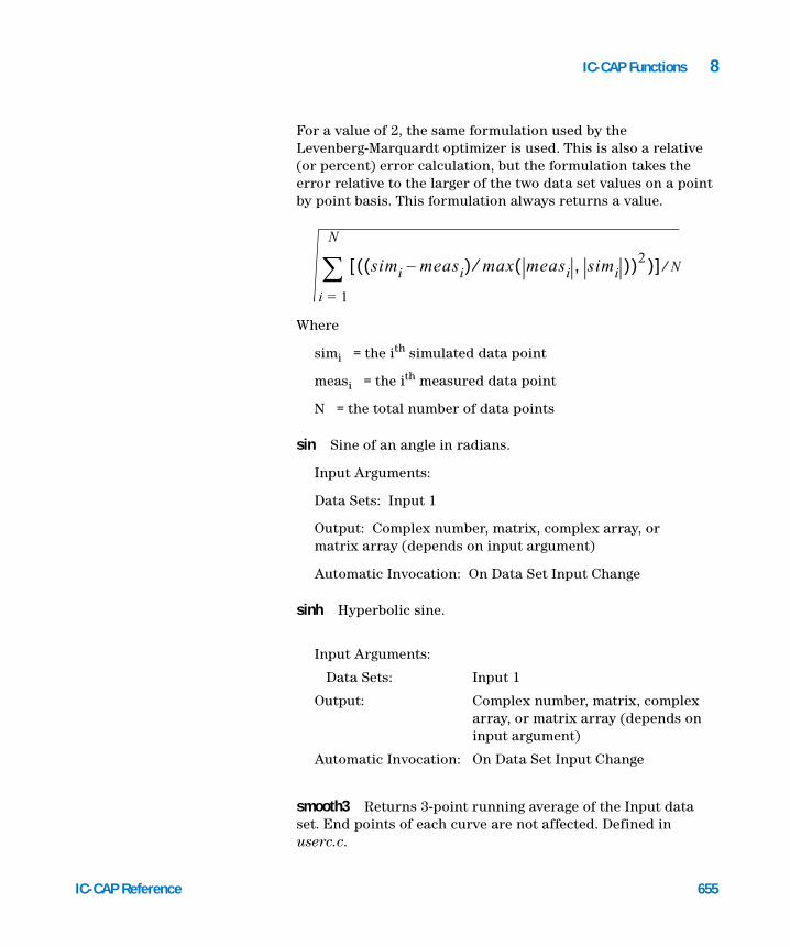
IC-CAP Functions 8
IC-CAP Reference
For a value of 2, the same formulation used by the Levenberg-Marquardt optimizer is used. This is also a relative (or percent) error calculation, but the formulation takes the error relative to the larger of the two data set values on a point by point basis. This formulation always returns a value.
Where
simi = the ith simulated data point
measi = the ith measured data point
N = the total number of data points
sin Sine of an angle in radians.
Input Arguments:
Data Sets: Input 1
Output: Complex number, matrix, complex array, or matrix array (depends on input argument)
Automatic Invocation: On Data Set Input Change
sinh Hyperbolic sine.
smooth3 Returns 3-point running average of the Input data set. End points of each curve are not affected. Defined in userc.c.
Input Arguments:
Data Sets: Input 1
Output: Complex number, matrix, complex array, or matrix array (depends on input argument)
Automatic Invocation: On Data Set Input Change
simi measi–( ) max measi simi,( )⁄( )2 )[ ]
i 1=
N
∑ N⁄
655

656
8 IC-CAP Functions
SPECSSpin Used in an IC-CAP Macro to determine the matrix connections of the device under test. ICMSpin returns the matrix pin number that corresponds to a specified terminal index on the device. This function only returns valid data when IC-MS test execution is running. Refer to the IC-MS User’s Manual for more information on using ICMSpin.
Example PEL Statement:pin_num = ICMSpin(1)
sqrt Square root function. Note that sqrt(-1) correctly produces an imaginary result.
Input Arguments:
Data Sets: Input
Output: Complex array or matrix array (depends on input argument)
Automatic Invocation: On Data Set Input Change
Input Arguments:
Reals or Integers: Terminal Index
Output: Matrix pin number corresponding to the specified device terminal index
Automatic Invocation: None
Input Arguments:
Data Sets: Input 1
Output: Complex number, matrix, complex array, or matrix array (depends on input argument)
Automatic Invocation: On Data Set Input Change
IC-CAP Reference

IC-CAP Functions 8
IC-CAP Reference
SWM_debug Switching matrix function. Turns the debug flag on and off. For more information regarding this function, refer to “External Matrix Driver User Functions” on page 168.
SWM_init Switching matrix function. Initializes the switching matrix and clears all port and pin connections. This must be called before any other switching matrix functions are used in the Macro. For more information regarding this function, refer to “External Matrix Driver User Functions” on page 168.
tan Tangent of an angle in radians.
tanh Hyperbolic tangent.
Input Arguments:
Reals or Integers: Debug Flag
Output: Single number with exit status
Automatic Invocation: None
Input Arguments:
Reals or Integers: Block 1 Addr, Block 2 Addr
Strings/Pars/Vars: Matrix Type, Device File
Output: Single number with exit status
Automatic Invocation: None
Input Arguments:
Data Sets: Input 1
Output: Complex number, matrix, complex array, or matrix array (depends on input argument)
Automatic Invocation: On Data Set Input Change
657

658
8 IC-CAP Functions
TARGET_DC_vth Picks up one single sweep curve of id=f(vg) of a specified setup and extracts the threshold voltage vth. The setup is specified by the parameters path to vd, and so on. This makes it easier to call the function with variable inputs inside the PEL programs.
The Flag variable defines certain conditions, for example, the extraction of vth for the large, which does not need to calculate all the early voltages.
Input Arguments:
Data Sets: Input 1
Output: Complex number, matrix, complex array, or matrix array (depends on input argument)
Automatic Invocation: On Data Set Input Change
Input Arguments:
Variable Length (L) Total gate width (W)Number fingers (NF)Flag for extraction options
flag: 1 Fixed Id(Vth) = Idref*L/W2 Fixed Id(Vth) = Idref*NF*
((W/NF)-2*Delta_W)/(L-2*Delta_L)
Reference current Idref forextraction options
Delta L (one side)Delta W (one side)# of curve Type (1=NMOS, -1=PMOS)Debug (1: show internal states of
the function 0: nothing)
IC-CAP Reference

IC-CAP Functions 8
IC-CAP Reference
tis_p_down HP 4071A wafer prober function. Lowers the chuck of the wafer prober.
tis_p_home HP 4071A wafer prober function. Used for loading a wafer onto the chuck and moving it to the home position.
tis_p_imove HP 4071A wafer prober function. Moves the chuck a relative increment from its current position.
tis_p_ink HP 4071A wafer prober function. Calls the inker function of the prober if it is supported.
tis_p_move HP 4071A wafer prober function. Moves the chuck to an absolute position.
tis_p_orig HP 4071A wafer prober function. Defines the current X & Y position of the chuck. Must be called before calling the tis_p_move or tis_p_imove functions.
tis_p_pos HP 4071A wafer prober function. Returns the current X & Y position of the chuck.
tis_p_scale HP 4071A wafer prober function. Defines the X and Y stepping dimensions that are used by the tis_p_move and tis_p_imove functions.
tis_p_up HP 4071A wafer prober function. Moves up the chuck of the wafer prober.
Parameters: path to setupvdvgvbidtype id (M,S)version
Output: Value vth or failure indicator
Automatic Invocation: Vth (1e99 indicates error)
659

660
8 IC-CAP Functions
tis_prober_get_ba HP 4071A wafer prober function. No Help Available.
tis_prober_get_name HP 4071A wafer prober function. No Help Available.
tis_prober_init HP 4071A wafer prober function. Initializes the prober for use. This function must be called before any other prober functions are used in the Macro.
tis_prober_read_sysconfig HP 4071A wafer prober function. No Help Available.
tis_prober_reset HP 4071A wafer prober function. Sends a device clear command to the prober.
tis_prober_status HP 4071A wafer prober function. Sends a query to the prober to obtain the Remote/Local control state and the edge sensor contact state. The prober should be initialized with tis_prober_init before this function.
TRL_Cal Deembed the raw measured data using measured data of TRL (thru-reflect-line) calibration standards. The function calculates the error coefficients and returns the corrected S-parameters data. The reference plane is defined at the middle of the thru standard, or at the interface to the DUT when it is installed in the compatible carrier.
IC-CAP Reference

IC-CAP Functions 8
IC-CAP Reference
TwoPort Converts the data in a data set from one 2-port parameter type (S, Y, H, Z, K, A) to another. Enter the name of the data set that is to be converted, the old 2-port type, and the new 2-port type. Use K for Cascaded Scattering Matrix and A for ABCD Matrix. Note: TWOPORT does not read TWOPORT_Z0 at execution time, only at measurement and simulation time.
Example PEL Statement:h_dataset = TwoPort(s_dataset,"S","H")
Inputs:
Freq Data: S data: Thru:
Short:
Line A:
Line B:
Line C:
Freq 1 Trans: Freq 2 Trans:
Frequency InputsRaw (uncalibrated) S-parametersmeasured S-parameters of the Thru standardmeasured S-parameters of the Short standardmeasured S-parameters of Line A standardmeasured S-parameters of Line B standardmeasured S-parameters of Line C standardtransition frequency Line A to Line Btransition frequency Line B to Line C
Output: Corrected (calibrated) S-parameters data
Input Arguments:
Data Sets: Input
Strings/Pars/Vars: From [SYHZKA], To [SYHZKA]
Output: Matrix array; size determined by inputs
Automatic Invocation: On Data Set Input Change
661

662
8 IC-CAP Functions
TwoPort2 Same as TwoPort function except the characteristic impedance, Z0, is an input parameter. This allows execution-time conversion of 2-port data to a new Z0.
Example PEL Statement:h_dataset = TwoPort2(s_dataset,75,"S","H")
USERC_avg_2 Averages 2 DC data sets, point-by-point. Provided as an example of a math function implemented in User C code. The source code is in $ICCAP_ROOT/src/userc.c.
USERC_avg_3 Averages 3 DC data sets, point-by-point. Provided as an example of a math function implemented in User C code. The source code is in $ICCAP_ROOT/src/userc.c.
Input Arguments:
Data Sets: Input
Reals or Integers: Z0
Strings/Pars/Vars: From (SYHZKA) To (SYHZKA)
Output: Matrix array; size determined by inputs
Automatic Invocation: On Data Set Input Change
Input Arguments:
Data Sets: Data 1, Data 2
Output: Array of real numbers; size determined by inputs
Automatic Invocation: On Data Set Input Change
Input Arguments:
Data Sets: Data 1, Data 2, Data 3
Output: Array of real numbers; size determined by inputs
Automatic Invocation: On Data Set Input Change
IC-CAP Reference

IC-CAP Functions 8
IC-CAP Reference
USERC_close Closes an open file. See USERC_open for essential additional information about this function.
USERC_conjg Produces the conjugate of the input data set. This function is similar to the function named conjg, but is provided as an example of a User C math function manipulating complex numbers. The source code is in $ICCAP_ROOT/src/userc.c.
USERC_data_w_check Returns a complex number designated by a name, row, and column. Example of C library function data_w_check() in userc.c.
Input Arguments:
Reals or Integers: File Descriptor (generated by earlier USERC_open call)
Output: 0 or -1 (-1 indicates an error)
Automatic Invocation: None
Input Arguments:
Data Sets: Cplx DS
Output: Complex number or array of complex numbers; size determined by inputs
Automatic Invocation: On Data Set Input Change
Input Arguments:
Reals or Integers: Row, Col, Index, Data Set name, Type
Output: A single complex number.
Automatic Invocation: None
663

664
8 IC-CAP Functions
USERC_get_object_name If the variable name exists, returns the name of the calling Transform or Macro. Note that the leading / in the name is not returned.
SyntaxUSERC_get_object_name(<varname>)
Where
<varname> is a string naming a variable in the variable table within the scope of the caller. This variable returns the names of the calling Transform or Macro.
Examples:
If macro /npn/tester contains the following line:x=USERC_get_object_name("objname")
And if objname is in the Model Variables or system variables, then it returns npn/tester.
If Transform /npn/dc/fgummel/tester contains the following line:
x=USERC_get_object_name("xformName")
And if xformName exists in the Setup Variables, DUT Variables, Model Variables, or System Variables, then it returns npn/dc/fgummel/tester.
USERC_init_param Demonstrates in C code how to assign a value to a model parameter, a DUT parameter, or an IC-CAP system variable. Demonstrates use of the User C utility function named set_par_or_var(). The source code is in the set_param function in $ICCAP_ROOT/src/userc.c.
Input Arguments:
Reals or Integers: New Value
Strings/Pars/Vars: Parameter to set (this should be the name of a model parameter, a DUT parameter, or an IC-CAP system variable)
Output: None
Extracts: N/A
IC-CAP Reference
IC-CAP Functions 8
IC-CAP Reference
USERC_num_of_points Returns the number of points for a given sweep. Example of C library function get_num_of_points() in userc.c.
Example PEL Statement:nop = USERC_num_of_points(1, "") ! A blank path is current Setup
USERC_open Accesses a disk file for reading, writing or both. For instrument control, use HPIB_open() and related HPIB functions. This function can be used in conjunction with USERC_readnum, USERC_readstr, USERC_read_reals, USERC_seek, USERC_tell, USERC_write, and USERC_close to perform I/O operations. A more complete description of these functions and examples of their use in performing I/O operations with disk files are available in Appendix H, “User C Functions.” The source code for these functions is provided in $ICCAP_ROOT/src/userc_io.c.
Example PEL Statement:file_num = USERC_open("datafile","r") ! read access
Automatic Invocation: By Extract menu function
Input Arguments:
Reals or Integers: Sweep order, Sweep path
Output: A positive real number, or -1 for error.
Automatic Invocation: None
Input Arguments:
Strings/Pars/Vars: Filename, Access Mode
Output: -1 on failure, or else a positive integer file designator that you should save to use with the other User C I/O functions mentioned in the description.
Automatic Invocation: None
665
666
8 IC-CAP Functions
USERC_read_reals Opens a file, reads and returns an array of real numbers, and closes the file. For additional information about this function, see Appendix H, “User C Functions.”
Example PEL Statement:data_array = USERC_read_reals("datafile")
USERC_readnum Reads 1 real number from an open file, 1.0E6, for example. See USERC_open for essential additional information about this function.
Example PEL Statement:VTO = USERC_readnum(file_num,0,"VTO = %lf")
USERC_readstr Reads a string from an open file and sets the specified IC-CAP variable equal to it. See USERC_open for essential additional information about this function.
Input Arguments:
Strings/Pars/Vars: Filename
Output: Array of real numbers, with size determined by the Setup
Automatic Invocation: None
Input Arguments:
Reals or Integers: File Descriptor (generated by earlier USERC_open call), Device File Flag
Strings/Pars/Vars: Scanf Format
Output: a real number (the value 9.99998E+37 means an error occurred)
Automatic Invocation: None
Input Arguments:
IC-CAP Reference

IC-CAP Functions 8
IC-CAP Reference
Example PEL Statement:! read and set SIMULATOR name from a file read_result = USERC_readstr(file_num,0,"%s",
IC-CAP_variable)
USERC_seek Goes to a particular byte offset in an open file. See USERC_open for essential additional information about this function.
USERC_set_param Sets the parameter specified by the second argument to the value of the first argument.
Example PEL Statement:
Reals or Integers: File Descriptor (generated by earlier USERC_open call), Device File Flag (use 1 if reading from an instrument driver device file, 0 if reading from an ASCII file)
Strings/Pars/Vars: Scanf Format, Var Name
Output: 0 on success, or -1 on failure
Automatic Invocation: None
Input Arguments:
Reals or Integers: File Descriptor (generated by earlier USERC_open call), Offset Value, Offset Type
Output: 0 on success, or -1 on failure
Automatic Invocation: None
Input Arguments:
Data Sets: None
Reals or Integers: Value of the parameter
Strings/Pars/Vars: Name of the parameter to set
Output: None
Automatic Invocation: MANUAL
667

668
8 IC-CAP Functions
x = USERC_set_param(100,NPN,BF)
USERC_set_param_quiet set the value of a parameter or variable referenced by a string. Unlike USERC_set_param(), this version makes no output to the status window.
Example PEL Statement:x=USERC_set_param_quiet(1e-15,"/npn/IS")
USERC_size Returns the array size of the data set whose name is given by a string.
Example PEL Statement:data_size = USERC_size("id")
USERC_sweep_mode Returns the sweep mode for the input with sweep order N.
Input Arguments:
Strings/Pars/Vars: Data Set name
Output: A positive real number.
Automatic Invocation: None
Usage: x=USERC_sweep_mode(N, <path>)
Returns: 0 for V1 for I2 for T3 for F4 for P5 for U6 for W
Extracts: Example C library function of get_sweep_mode() in userc.c. Use USERC_num_of_points() to check the existence of a sweep.
IC-CAP Reference

IC-CAP Functions 8
IC-CAP Reference
USERC_sweep_name Returns a sweep name through a variable. Example C library function of get_sweep_name() in userc.c. Use USERC_num_of_points() to check the existence of a sweep.
Example PEL Statement:x = USERC_sweep_name(1, "/npn/dc/fearly", "first_sweep")
USERC_sweep_start Returns a sweep start value. Example C library function of get_sweep_start() in userc.c. Use USERC_num_of_points() to check the existence of a sweep.
Example PEL Statement:x = USERC_sweep_start(1, "/npn/dc/fearly")
USERC_sweep_stepsize Returns a (LIN) sweep step value. Example C library function of get_sweep_stepsize() in userc.c. Use USERC_num_of_points() to check the existence of a sweep.
Example PEL Statement:x = USERC_sweep_stepsize(1, "/npn/dc/fearly")
Input Arguments:
Strings/Pars/Vars: Sweep order, Sweep path, Variable name
Output: 0 for success, -1 for error
Automatic Invocation: None
Input Arguments:
Strings/Pars/Vars: Sweep order, Sweep path
Output: 0 for error
Automatic Invocation: None
Input Arguments:
Strings/Pars/Vars: Sweep order, Sweep path
Output: 0 for error
Automatic Invocation: None
669

670
8 IC-CAP Functions
USERC_sweep_stop Returns a sweep stop value. Example C library function of get_sweep_stop() in userc.c. Use USERC_num_of_points() to check the existence of a sweep.
Example PEL Statement:x = USERC_sweep_stop(1, "") ! within current Setup
USERC_system Demonstrates the invocation of an operating system command from User C code.
USERC_tell Tells current byte offset in an open file. See USERC_open for essential additional information about this function.
Input Arguments:
Strings/Pars/Vars: Sweep order, Sweep path
Output: 0 for error.
Automatic Invocation: None
Input Arguments:
Strings/Pars/Vars: operating system command
Output: Single number with exit status of the operating system command
Automatic Invocation: None
Input Arguments:
Reals or Integers: File Descriptor (generated by earlier USERC_open call)
Output: −1 on error, or else current byte offset into file
Automatic Invocation: None
IC-CAP Reference

IC-CAP Functions 8
IC-CAP Reference
USERC_transpose Returns a data set of matrices, in which each of the input data set’s matrices has been transposed. Provided as an example of a matrix math function implemented in User C code. The source code is in $ICCAP_ROOT/src/userc.c.
USERC_write Prints any string expression into an open file, in ASCII. (To convert a number to a string expression, refer to the VAL$ function described in the “Built-in Functions” on page 714. Refer to USERC_open for additional essential information about this function.)
Example PEL Statement:write_result = USERC_write(file_num,0,"VTO="&VAL$(VTO))
variance Calculates the statistical variance of a data set. Adequate for a real or complex data set, but if a data set of matrices is received, only the 1,1 data is considered. A data set specification like S.21 is adequate, since this is a data set of complex numbers.
Input Arguments:
Data Sets: Matrix DS
Output: Matrix or matrix array; size determined by inputs
Automatic Invocation: On Data Set Input Change
Input Arguments:
Reals or Integers: File Descriptor (generated by USERC_open call), Device File Flag
Strings/Pars/Vars: String to Write
Output: 0 or −1 (−1 indicates an error)
Automatic Invocation: None
Input Arguments:
Data Sets: Input 1
671

672
8 IC-CAP Functions
VBIC_ac_solver Given the 4 terminal voltages, solves for 2-port network parameters. VE and VS are assumed to be 0.
VBIC_avc Calculates avalanche collector voltage (AVC1) based on the model parameter PC.
Where
For an NPN, a = 7.05E05 cm-1 and b = 1.23E06 V/cm
For a PNP, a = 1.58E06 cm-1 and b = 2.04E06 V/cm
PC = b-c grading coefficient
Output: Single real or complex number
Automatic Invocation: On Data Set Input Change
Input Arguments:
VC (Collector Voltage)
VB (Base Voltage)
FREQ (Cut-off Frequency])
Output {FT|BETA|Y|H|Z|S}
Output code specifying current gain, or parameters. This code should be placed in the Output field.
Outputs: The output depends on the code set in the Output field:
Code Output
FT Current gain cutoff frequency
BETA Current gain
Y The 2-port network y-parameters
H The 2-port network h-parameters
Z The 2-port network z-parameters
S The 2-port network s-parameters
AVC1a
b 1 PC–( )-------------------------=
IC-CAP Reference

IC-CAP Functions 8
IC-CAP Reference
VBIC_cbc Calculates the depletion capacitance versus bias.
VBIC_cbe Calculates the depletion capacitance versus bias.
VBIC_cj0 Calculates (extracts) the junction zero-bias capacitance.
Input Arguments: None
Output: Model parameter AVC1
Input Arguments:
VBC Base-Collector Voltage
Output: Depletion base-collector capacitance based on the VBIC formulation: SPICE model for AJC ≤ 0 and single-piece smooth model for AJC > 0.
Input Arguments:
VBE Base-Emitter Voltage
Output: Depletion base-emitter capacitance based on the VBIC formulation: SPICE model for AJC ≤ 0 and single-piece smooth model for AJC > 0.
Input Arguments:
VJ Junction voltage
CJ Capacitance
Output: E/C/S Junction {E|C|S} for CJE, CJC, or CJCP
Output: The zero-bias junction capacitance stored in CJE, CJC, or CJCP.
673

674
8 IC-CAP Functions
VBIC_clean_data This routine looks at each data point and scans ahead by the number of points specified by the input argument IN A ROW. If the data does not monotonically increase for the number of data points specified by IN A ROW, then zero is written to the output array. If the data does monotonically increase for the number of data points specified by IN A ROW, then from that data point onward, the INPUT DATA is written directly to the output (result) array.
VBIC_csc Calculates the depletion capacitance versus bias.
VBIC_dc_approx This function calculates Ic, Ib, beta, intrinsic and extrinsic base-emitter voltage, and base charge for a bipolar transistor, using the terminal voltages Ve, Vb, and Vc as inputs. Vs is assumed to be 0. The first parameter should be set to the output of interest, which defaults to Ic. This approximate solution does not take quasi-saturation effects into account.
Input Arguments:
INPUT DATA
IN A ROW
Output: Either the INPUT DATA or zero values.
Input Arguments:
VSC (Substrate-Collector Voltage)
Output: Depletion collector-substrate capacitance based on the VBIC formulation: SPICE model for AJC ≤ 0 and single-piece smooth model for AJC>0.
Input Arguments:
VC Collector Voltage
IC-CAP Reference

IC-CAP Functions 8
IC-CAP Reference
VBIC_dci_solver This function calculates Ic, Vb, Ie, Is, or beta for a bipolar transistor, using the terminal voltages Ve, Vc, and Vs and Ib as inputs. The first parameter should be set to the output of interest, which defaults to Ic.
VB Base Voltage
VE Emitter Voltage
Output:IC|IB|BETA|VBEI|VBEX|QB
Set this field to the output of interest
Output: The output depends on the setting of the Output field.
Code Output
IC Collector current
IB Base current
BETA Current gain
VBEI Intrinsic base-emitter voltage
VBEX Extrinsic base-emitter voltage
QB Base charge
Input Arguments:
VC Collector Voltage
IB Base Current
VE Emitter Voltage
VS Substrate Voltage
Output: IC|VB|IE|IS|BETA
Set this field to the output of interest.
Output: The output depends on the code set in the Output field.
Code Output
675

676
8 IC-CAP Functions
VBIC_dcv_solver This function calculates Ic, Ib, Ie, Is, or beta for a bipolar transistor, using the terminal voltages Ve, Vb, Vc, and Vs as inputs. The first parameter should be set to the output of interest, which defaults to Ic.
VBIC_fg_currents Given the 4 terminal voltages, calculates parameters related to forward current.
IC Collector current
VB Base voltage
IE Emitter current
IS Substrate current
BETA Current gain
Input Arguments:
VC Collector Voltage
VB Base Voltage
VE Emitter Voltage
VS Substrate Voltage
Output: IC|IB|IE|IS|BETA
Set this field to the output of interest.
Output: The output depends on the code set in the Output field:
Code Output
IC Collector current
VB Base voltage
IE Emitter current
IS Substrate current
BETA Current gain
IC-CAP Reference

IC-CAP Functions 8
IC-CAP Reference
Input Arguments:
Data Sets: VC Collector VoltageVB Base VoltageVE Emitter VoltageVS Substrate VoltageIC Collector CurrentIB Base Current
Parameters: The parameter indicates the region where the transform will limit its simulated output. VBIC_AUTO_RANGE must be set to 1.
IS|NF Calculate over the region dominated by NF
IBEI|NEI Calculate over the region dominated by NEI
IBEN|NEN Calculate over the region dominated by NEN
IKF Calculate over the region dominated by IKF
Output: {IB|B|IC|C|IE|E|IS|S}
Code to indicate which current to output.
Output: A subset of the current where zeros replace any range where data was not extracted (based on the auto-ranging algorithm). The output depends on the code set in the Output field:
Code Output
IB|B Base current
IC|C Collector current
IE|E Emitter current
IS|S Substrate current
677

678
8 IC-CAP Functions
VBIC_ibci_nci Calculates the parameters IBCI and NCI.
VBIC_ibei_nei Calculates the parameters IBEI and NEI.
VBIC_ikf Calculates the parameter IKF.
Extracts: Nothing
Input Arguments:
VB Base Voltage
VC Collector Voltage
IB Base Current
Output: NCI at each bias point (unaveraged).
Extracts: IBCI, NCI
Input Arguments:
VB Base Voltage
VE Emitter Voltage
IB Base Current
Output: NEI at each bias point (unaveraged).
Extracts: IBEI, NEI
Input Arguments:
VB Base Voltage
VE Emitter Voltage
IC Collector Current
IB Base Current
Output: IKF at each bias point
IC-CAP Reference

IC-CAP Functions 8
IC-CAP Reference
VBIC_ikr Calculates the parameter IKR.
VBIC_is_nf Calculates the parameters IS and NF.
VBIC_isp_nfp Calculates the parameters ISP and NFP.
Extracts: IKF (maximum value in range, 0.1 indicates failed extraction).
Input Arguments:
VB Base Voltage
VC Collector Voltage
IE Emitter Current
IB Base Current
Output: Reverse beta versus bias.
Extracts: IKR (maximum value in range, 0.1 indicates failed extraction).
Input Arguments:
VB Base Voltage
VE Emitter Voltage
IC Collector Current
Output: NF versus bias with 0’s where out of auto-range.
Extracts: IS, NF (average values in range).
Input Arguments:
VB Base Voltage
VC Collector Voltage
IS Substrate Current
Output: NFP versus bias with 0’s where out of auto-range.
679

680
8 IC-CAP Functions
VBIC_nr Calculates the parameter NR.
VBIC_qcdepl Calculates depletion charge or capacitance based on VBIC formulation using SPICE model for A ≤ 0 and single-piece, smooth model for A > 0.
VBIC_rcx Calculates RCX.
Extracts: ISP, NFP (average values in range).
Input Arguments:
VB Base Voltage
VC Collector Voltage
IE Emitter Current
Output: NR versus bias with 0’s where out of auto-range.
Extracts: NR (average value in range).
Input Arguments:
Junction V Junction voltage
P Param Built-in potential
M Param Grading coefficient
F Param Fwd bias depletion capacitance limit
A Param Smoothing factor
Mode : {Q|C} Charge or capacitance
Output: Charge or capacitance versus bias.
Extracts: Nothing
Input Arguments:
VB Base Voltage
VE Emitter Voltage
IC-CAP Reference

IC-CAP Functions 8
IC-CAP Reference
VBIC_rg_currents Given the 4 terminal voltages, calculates reverse currents.
IC Collector Current
IS Substrate Current
IB Base Current
Output: RCX versus bias with 0’s where out of auto-range.
Extracts: RCX (maximum value in auto-range, if failed, value of 60 set).
Input Arguments:
VC Collector Voltage
VB Base Voltage
VE Emitter Voltage
VS Substrate Voltage
IE Emitter Current
IB Base Current
IS Substrate Current
Parameters The parameter indicates the region where the transform will limit its simulated output. VBIC_AUTO_RANGE must be set to 1.
IS|NR Calculate over the region dominated by NR
IBCI|NCI Calculate over the region dominated by NCI
IBCN|NCN Calculate over the region dominated by NCN
IKR Calculate over the region dominated by IKR
681

682
8 IC-CAP Functions
VBIC_stoc This function calculates capacitance data from S-parameter data, allowing base-collector and base-emitter capacitance to be calculated from network analyzer measurements. The output of this function can be used in place of actual capacitance data to extract capacitance-related parameters.
ISP|NFP Calculate over the region dominated by NFP
IKP Calculate over the region dominated by IKP
Output: {IB|B|IC|C|IE|E|IS|S}
Code to indicate which current to output.
Output: A subset of the current where zeros replace any range where data was not extracted (based on the auto-ranging algorithm).
The output depends on the code set in the Output field:
Code Output
IB|B Base current
IC|C Collector current
IE|E Emitter current
IS|S Substrate current
Extracts: Nothing.
Input Arguments:
FREQ data Frequency
S data S-parameter data (de-embedded)
Node (C/E/S) Code to indicate type of extraction:E base-emitter capacitanceC base-collector capacitanceS substrate-collector capacitance
IC-CAP Reference

IC-CAP Functions 8
IC-CAP Reference
VBIC_vef_ver Calculates the forward and reverse early voltages given the collector, base, and emitter voltages in the forward and reverse modes, as well as the collector current in the forward mode and the emitter current in the reverse mode. The algorithm is based on the method described in “SPICE Early Modeling” by C. McAndrew & L. Nagel, BCTM 94, p. 144.
Wait Switching matrix function. Used to pause for a specified number of seconds to accomplish dry switching. Refer to Chapter 2, “MOSFET Characterization,” in the IC-CAP Nonlinear Device Models, Volume 1 manual for more information.
Output: Capacitance versus frequency data
Extracts: Nothing
Input Arguments:
Forward VC Collector Voltage
Forward VB Base Voltage
Forward VE Emitter Voltage
Forward IC Collector Current
Reverse VE Emitter Voltage
Reverse VB Base Voltage
Reverse VC Collector Voltage
Reverse IE Emitter Current
Forward IB Base Current
Output: VEF versus bias with 0’s where out of auto-range.
Extracts: VEF, VER (average values in auto-range).
Input Arguments:
Reals or Integers: Period [sec]
683

684
8 IC-CAP Functions
wirexfX A wire function. Wire functions permit optimization of time-domain measurements in the X and Y dimensions. Time-domain measurements involve effects specifically related to the Y axis (voltage or current level) or the X axis (when a pulse occurs).
Because X-axis data is typically the forced data set, it cannot normally be optimized. This makes it very difficult to optimize measured and simulated pulses that do not start with some amount of overlap in time. To solve this problem, the data can be transformed to create an independent X data set that can be optimized together with the Y data set. There are 2 ways of doing this.
• Generate the set of X values that would result if the Y values were evenly spaced. The wirexfX provides this data. The complementary wirexfY function provides the set of Y values that would result from evenly spaced X values, which is the default case.
• Generate the sets of X and Y values that would result if the X and Y axes are normalized and the curve is divided into segments of equal length. The wirexfXY and wirexfYX functions provide this data. This function calculates variably spaced X values for evenly spaced Y values.
wirexfXY One of the wire functions that permit optimization of time domain measurements in the X and Y dimensions; for more details, refer to the wirexfX function. This function calculates the X data set produced when the X and Y axes are
Output: Single number with exit status
Automatic Invocation: None
Input Arguments:
Data Sets: X Data, Y Data
Output: Array of real numbers; size determined by inputs
Automatic Invocation: On Data Set Input Change
IC-CAP Reference

IC-CAP Functions 8
IC-CAP Reference
normalized and the curve is divided into segments of equal length. This function should be used in conjunction with wirexfYX during an optimization.
wirexfY One of the wire functions that permit optimization of time domain measurements in the X and Y dimensions; for more details, refer to the wirexfX function. This function calculates the Y data set when X values are evenly spaced. This function is supplied for completeness because Y data sets are normally collected in this manner.
wirexfYX One of the wire functions that permit optimization of time domain measurements in the X and Y dimensions; for more details, refer to the wirexfX function. This function calculates the Y data set produced when the X and Y axes are normalized and the curve is divided into segments of equal length. This function should be used in conjunction with wirexfXY during an optimization.
Input Arguments:
Data Sets: X Data, Y Data
Output: Array of real numbers; size determined by inputs
Automatic Invocation: On Data Set Input Change
Input Arguments:
Data Sets: X Data, Y Data
Output: Array of real numbers; size determined by inputs
Automatic Invocation: On Data Set Input Change
Input Arguments:
Data Sets: X Data, Y Data
Output: Array of real numbers; size determined by inputs
685

686
8 IC-CAP Functions
Automatic Invocation: On Data Set Input Change
IC-CAP Reference

Agilent 85190A IC-CAP 2008Reference
9Parameter Extraction Language
Fundamental Concepts 688
Expressions 748
IC-CAP’s Parameter Extraction Language can be used to create new functions. This language is modeled on Rocky Mountain BASIC (rmb), the name adopted for HP BASIC or Workstation BASIC when HP introduced it on HP-UX. IC-CAP implements a subset that can aid in controlling the system and performing computations.
This chapter describes the syntax and operation of this interpreter. It is responsible for several IC-CAP system features:
• Numerical expressions in most editors in the system
• Transforms using the Program2 or Program function
• Macros that a Model can use
687Agilent Technologies

9 Parameter Extraction Language
Fundamental Concepts
688
The interpreter within IC-CAP can execute programs made up of statements that consist of keywords and expressions. Expressions are constructed from functions, identifiers, and operators. You enter these statements in the text editor that appears when you select Program2 or Program as the function name in the Extract/Optimize folder, or when you open the Macros folder (refer to Chapter 11, “Creating and Running Macros,” in the IC-CAP User’s Guide). The same interpreter is used to evaluate the expressions entered in various tables providing a consistent syntax throughout the system. Strictly speaking, the expressions appearing in tables are not statements.
Keywords
Keywords are reserved by the Parameter Extraction Language. A keyword can be one of the reserved words required for a statement, such as PRINT.
It can also be a built-in function or a built-in constant. For keyword descriptions, refer to “Built-in Functions” on page 714 and “Built-In Constants” on page 747.
Keywords are entered in all uppercase or all lowercase, but not upper and lower case. For example, to call the built-in function MAX:MAX(ic) or max(ic)
Although the functions in IC-CAP’s Function List can be invoked, those functions, such as RMSerror, are not language keywords. To be used in a Program, expression, or Macro, these functions must be spelled exactly as shown in the Function List.
Identifiers
Identifiers are Parameter Extraction Language variable names; they have the following properties:
• Identifiers can be of mixed case.
IC-CAP Reference

Parameter Extraction Language 9
IC-CAP Reference
• An identifier can be any length.
• An identifier starts with an alphabetic character or an underscore character ( _ ). It can include alphanumeric characters and underscore characters thereafter. Four notable exceptions to this are:
• A subcircuit parameter, like npn.BF, is a legitimate identifier; a period (.) is allowed in this case.
• A data set, like npn/dc/fgummel/ic is a legitimate identifier; a slash (/) is allowed in this case.
• The notations ../ and ../.. are allowed to indicate relative paths in the currently executing macro or transform for dataset access.
• In Programs and Macros, local variable names (identifiers) can end with a trailing dollar sign ($). Included for the convenience of BASIC programmers when using string variables, the only effect is that the program is easier to read. An example is: Hi$="hello world"
Numeric Precision
You can control numeric precision by setting the variables WORKING_PRECISION and/or PARAMETER_PRECISION or by using the PEL function val$().
• PARAMETER_PRECISION
This variable controls the precision of parameters stored in the Model or DUT Parameters table, as well as the precision of parameters passed to a simulator.
• WORKING_PRECISION
This variable controls the precision of numeric values when converted to text, but affects only those parts of a model for which the variable is defined. Depending on when and where the conversion occurs, precision can be actually lost or simply hidden. This conversion occurs in the following situations: any time the function val$() is called; the PRINT statement is used; a numeric value is
689

690
9 Parameter Extraction Language
assigned to a variable in the IC-CAP Variable Table; a number is displayed to the screen (e.g., in an input/output/plot definition or tabular data) or saved to a file. (Because all variables in the IC-CAP Variable Table are text by definition, assigning a numeric value to such a variable will implicitly call the val$() function.)
Although the numbers are truncated for display purposes according to the WORKING_PRECISION variable, IC-CAP uses the untruncated numbers for calculations until the file is saved. After the truncated numbers are saved in a file then reread, the truncated numbers are used in calculations. For example, if you type 1.23456 into an input field, 1.235 is displayed. However, 1.23456 is used for calculation. After the file is saved and reread, 1.235 is not only displayed but also used for calculations.
When you change the WORKING_PRECISION variable, the change is only apparent with subsequently edited or redisplayed fields.
The value of the WORKING_PRECISION variable applies to the precision of the Start/Stop/Stepsize fields of inputs, though not all instrumentation can support such resolution. Using higher precision involving these fields should be done with caution.
The range of values is 6 through 17. The default is 6.
Controlling precision through val$() calls
The function val$() has an optional second argument that can be used to control numeric precision. For example, the statement y=val$(x,12) will convert the number x to a string using up to 12 significant digits if required. Use this form of val$() when the current value of WORKING_PRECISION is acceptable for most of the work at hand, but greater control is required for isolated instances. In those instances, the second argument of val$() can be used to override the current working precision.
IC-CAP Reference

Parameter Extraction Language 9
IC-CAP Reference
The examples that follow show how the output varies based on whether or not the WORKING_PRECISION variable is defined, and how the WORKING_PRECISION variable, when defined, is overridden by using val$().
NOTE When doing comparisons on real numbers, you may see unexpected results (PEL printouts are rounded, although full precision is used internally). Using the new WORKING_PRECISION variable or the val$(xxx,y) function, you can verify the actual value.
For example, consider the following PEL clause:x=0.39999999999IF x < 0.4 THEN
PRINT x;“is less than 0.4”END IF
Since x=0.39999999999, the IF clause will be entered but it will print 0.4 is less than 0.4. To verify the actual value, change the x in the print statement to val$(x,15) . The output will then show 0.39999999999 is less than 0.4.PRINT val$(x,15);“is less than 0.4
Example, Scenario 1
This scenario shows the usefulness of the new argument in the val$() function.
Conditions: No WORKING_PRECISION variable is declared within current scope; var1, and var2 are variables in the Variable table within the current scope.
PEL
x=0.1234567890123 ! implicit val$() used behind the scenes usesvar1=x ! default working precision (6 digits)var2=val$(x,9) ! explicit val$() specifying 9 digits of precisiony=0+var1 ! implicit val() used on var1 to make numeric again z=0+var2 ! implicit val() used on var1 to make numeric again print “Default precision x=”,x ! default working precision used print “Default precision y=”,y ! default working precision used print “Default precision z=”,z ! default working precision used print “var1=”,var1 ! no conversion--var1 already textprint “var2=”,var2 ! no conversion--var2 already textprint “High precision x=”,val$(x,9) ! explicit working precision print “High precision y=”,val$(y,9) ! explicit working precision print “High precision z=”,val$(z,9) ! explicit working precision
691

692
9 Parameter Extraction Language
OutputDefault precision x= 0.1235Default precision y= 0.1235Default precision z= 0.1235var1= 0.1235var2= 0.123456789High precision x= 0.123456789High precision y= 0.1235High precision z= 0.123456789
Notice that y lost precision because var1 lost precision, however it is clear from the High precision lines that more information is available for x and z even though printing at the default precision did not reveal it.
Example, Scenario 2
This Scenario uses the same code as Scenario 1, except that the default working precision has been increased via the WORKING_PRECISION variable.
Conditions: WORKING_PRECISION variable in the current scope is set to 12; var1 and var2 are variables in the Variable Table within the current scope.
PEL
x=0.1234567890123 ! implicit val$() used behind the scenes usesvar1=x ! current working precision (12 digits)var2=val$(x,9) ! explicit val$() specifying 9 digits of precisiony=0+var1 ! implicit val() used on var1 to make numeric again z=0+var2 ! implicit val() used on var1 to make numeric again
print “Default precision x=”,x ! current working precision used print “Default precision y=”,y ! current working precision used print “Default precision z=”,z ! current working precision used print “var1=”,var1 ! no conversion--var1 already textprint “var2=”,var2 ! no conversion--var2 already textprint “High precision x=”,val$(x,9) ! explicit working precision print “High precision y=”,val$(y,9) ! explicit working precision print “High precision z=”,val$(z,9) ! explicit working precision
OutputDefault precision x= 0.123456789012 Default precision y= 0.123456789012 Default precision z= 0.123456789var1= 0.123456789012var2= 0.123456789High precision x= 0.123456789High precision y= 0.123456789High precision z= 0.123456789
IC-CAP Reference

Parameter Extraction Language 9
IC-CAP Reference
In this case, notice that the overriding val$() assignments actually lower the default precision since the default has been set to 12 digits via the WORKING_PRECISION variable.
Statements
This section describes how to write statements that make up Programs and Macros. The information in this section is not required to use expressions in the editor tables within IC-CAP.
Rules for Constructing Statements
As in BASIC, statements are generally contained in a single line of input. On the other hand, a quoted string can be as many lines long as needed and can contain CR-LFs (carriage return-line feeds).
Statements can be arbitrarily complex, and can use parentheses and white space to clarify precedence and improve readability.
Keywords must be all uppercase or all lowercase characters. Calls to functions in IC-CAP’s Function List must be spelled exactly as they are in the Function List.
Use an exclamation mark (!) to comment out a line or any part of a line.
Available Statements and Commands
The following statements are taken from HP BASIC. They are sensitive to the use of CR-LF, and must be written as shown. For example, the ELSE keyword should be followed by nothing on the same line, although a comment (starting with ! ) could follow it. In this section, the abbreviation expr denotes an expression. Expressions are described in “Expressions” on page 748. The abbreviation boolean_expr denotes a boolean expression, generally 0 or 1 (1, as well as any non-zero value, is considered TRUE). For more information, refer to “Boolean Expressions” on page 750.
693

694
9 Parameter Extraction Language
IF THEN with a single statementIF boolean_expr THEN statement
IF THEN with multiple statementsIF boolean_expr THEN statement1...statementNEND IF
IF THEN ELSE statementIF boolean_expr THEN statement1...statementNELSEstatement1...statementNEND IF
WHILE statementWHILE boolean_expr statement1...statementNEND WHILE
GET_DATASET statementGET_DATASET prompt_string, variable_nameGET_DATASET prompt_string, default_string, variable_name
GET_DATASET is currently only supported by the Program2 function. An error occurs if used with a Program function or Macro. GET_DATASET can redirect a Program2 dataset or array parameter argument into a named variable. The prompt_string and optional default_string parameters are currently unused and ignored. The variable_name argument is a variable that receives the redirected Program2 parameter argument. The named variable can be a variable local to the Program2 function. After the GET_DATASET statement finishes, it returns a dataset to the named variable. Currently the named variable can not represent a global variable or variable from an IC-CAP variable table.
IC-CAP Reference

Parameter Extraction Language 9
IC-CAP Reference
Example Program2 function transform using GET_DATASET: sub_prog{
PRINT "enter sub_prog"
! re-direct a dataset parameter argument passed into this
! function into local variable loc_xGET_DATASET "", loc_x
PRINT "loc_x == "PRINT loc_x
PRINT "leave sub_prog"RETURN
}
Example:! create a small dataset xCOMPLEX x[5]i = 0WHILE i < sizeof(x)
x[i] = i+2 + j*(i+1)i=i+1
ENDWHILE
! pass a small dataset x to the Program2 function sub_progiccap_func("sub_prog", "Execute", x)
Output:enter sub_progloc_x == Point Index R:measured I:measured
0 (1,1) 2.000000E+000 1.000000E+0001 (1,1) 3.000000E+000 2.000000E+0002 (1,1) 4.000000E+000 3.000000E+0003 (1,1) 5.000000E+000 4.000000E+0004 (1,1) 6.000000E+000 5.000000E+000
Point Index R:simulated I:simulated 0 (1,1) 2.000000E+000 1.000000E+0001 (1,1) 3.000000E+000 2.000000E+0002 (1,1) 4.000000E+000 3.000000E+0003 (1,1) 5.000000E+000 4.000000E+0004 (1,1) 6.000000E+000 5.000000E+000
leave sub_prog
GET_INT statementGET_INT prompt_string, variable_nameGET_INT prompt_string, default_string, variable_name
Uses a dialog box to request an integer input from the user, prompting with prompt_string, which should be a quoted string, an identifier, or an expression treated as an integer. Where applicable, default_string provides the user with a default answer, enabling the user to simply select OK and avoid typing any data. The prompt_string can be any valid
695

696
9 Parameter Extraction Language
string expression. The default_string can be any valid string expression representing an integer. The variable_name argument is a variable that receives the user's response. The variable can be an IC-CAP system variable, or a variable local to Program, Program2, or Macro. After the GET_INT statement finishes, it returns an integer value to the named variable. If the named variable is a global variable, the integer value will be stored in the variable table.
The GET_INT dialog box contains 2 buttons: CANCEL and OK. Choose CANCEL to terminate Program, Program2, or Macro immediately.
If GET_INT is used in a Program or Macro to pass parameters, all GET_INT statements should be located immediately at the start of the Program or Macro along with any other GET_INT, GET_REAL, GET_STRING or LINPUT statements. Once any other ICCAP_FUNC statement is invoked, the list of arguments is reset, thereby removing all the extra arguments from the calling ICCAP_FUNC statement. Program2 does not have this limitation.
If GET_INT is used in a Program or Macro to pass parameters, the GET_INT statement searches the passed parameter list until it finds a valid passed integer parameter argument. In the Program2 function, the GET_INT statement will only try to evaluate the next available passed function parameter as an integer value, and will error out if the next passed function parameter can not be evaluated as an integer value.
GET_REAL statementGET_REAL prompt_string, variable_name GET_REAL prompt_string, default_string, variable_name
Uses a dialog box to request a real input from the user, prompting with prompt_string, which should be a quoted string, an identifier, or an expression treated as a real value. Where applicable, default_string provides the user with a default answer, enabling the user to simply select OK and avoid typing any data. The prompt_string can be any valid string expression. The default_string can be any valid string expression representing a real value. The variable_name argument is a variable that receives the user's response. The
IC-CAP Reference

Parameter Extraction Language 9
IC-CAP Reference
variable can be an IC-CAP system variable, or a variable local to Program, Program2, or Macro. After the GET_REAL statement finishes, it returns a real value to the named variable. If the named variable is a global variable, the string value will be stored in the variable table.
The GET_REAL dialog box contains 2 buttons: CANCEL and OK. Choose CANCEL to terminate Program, Program2, or Macro immediately.
If GET_REAL is used in a Program or Macro to pass parameters, all GET_REAL statements should be located immediately at the start of the Program or Macro along with any other GET_INT, GET_REAL, GET_STRING or LINPUT statements. Once any other ICCAP_FUNC statement is invoked, the list of arguments is reset, thereby removing all the extra arguments from the calling ICCAP_FUNC statement. Program2 does not have this limitation.
If GET_REAL is used in a Program or Macro to pass parameters, the GET_REAL statement searches the passed parameter list until it finds a valid passed real parameter argument. In the Program2 function, the GET_REAL statement will only try to evaluate the next available passed function parameter as a real value, and will error out if the next passed function parameter can not be evaluated as a real value.
GET_STRING statement:
See “LINPUT or GET_STRING statement” on page 699. GET_STRING is simply an alternate name for the LINPUT command. The new name is consistent with GET_INT, GET_REAL, and GET_DATASET.
GLOBAL_VAR statementGLOBAL_VAR <variable_name>
Declares a variable as a global variable in a program. This statement is most useful for the Program2 function, because the Program2 function treats all variables as local variables unless those variables are first explicitly declared as global variables using the GLOBAL_VAR statement. In the Program
697

698
9 Parameter Extraction Language
function, all variables can be resolved globally or locally without needing to explicitly specify which variables are global using the GLOBAL_VAR statement.
The variable_name should refer to an IC-CAP variable in a variable table. Before using a variable from a variable table in Program2, you should declare the variable as global with GLOBAL_VAR. An error will occur if an IC-CAP variable could not be found.
GLOBAL_VAR varXy=varXRETURN y
ICCAP_FIND_CHILDREN statementICCAP_FIND_CHILDREN “/”,“Model”,loadedModels
Sets a variable to be the list of names of a particular child type of an IC-CAP object. This turns the variable loadedModels from a variable table into an ICCAP_ARRAY containing elements that are the names of the currently loaded models. Use the sizef() command to determine the size of the array.
Refer to the following table for valid names for the second argument given the type of the first argument.
First Argument References Second Argument may be
/ Model
any GUI Item Table or any GUI Item GUI Item
any model DUT
any DUT Setup
Any Setup Input, Output, Transform, or Plot
NOTE You should use sizeof() instead of size() because if no objects of the requested type are found, a null string ("") is returned instead of an ICCAP_ARRAY[0]. Since size() returns 1 for a null string, you would first test the result to make sure it is not a null string before using the size() command to determine the number of entries. The sizeof() function returns 0 for a variable that is not an ICCAP_ARRAY[].
IC-CAP Reference

Parameter Extraction Language 9
IC-CAP Reference
ICCAP_FUNC statementICCAP_FUNC (object_name, menu_function_name, dialog_answer1, ...)
Used primarily in macros for automating the operation of IC-CAP.
NOTE The ICCAP_FUNC statement replaced the MENU_FUNC statement in release 5.0. For backward compatibility, macros containing the MENU_FUNC statement will still work, but new macros should be written using the ICCAP_FUNC statement.
For an example on using the ICCAP_FUNC statement, refer to Chapter 11, “Creating and Running Macros,” in the IC-CAP User’s Guide.
LINPUT or GET_STRING statementLINPUT prompt_string, variable_name LINPUT prompt_string, default_string, variable_nameGET_STRING prompt_string, variable_nameGET_STRING prompt_string, default_string, variable_name
Uses a dialog box to request a string input from the user, prompting with prompt_string, which should be a quoted string, an identifier, or an expression treated as a string. Where applicable, default_string provides the user with a default answer, enabling the user to simply select OK and avoid typing any data. Like prompt_string, the default_string can be any valid string expression. The variable_name argument is a variable that receives the user’s response. The variable can be an IC-CAP system variable, or a variable local to the Program, Program2, or Macro. After the LINPUT or GET_STRING statement finishes, it returns a string to the named variable. This will either be the null string (""), or a string defining the text that would be typed in the LINPUT or GET_STRING dialog box. If the named variable is a global variable, the string value will be stored in the variable table. To interpret the results as a number, you must use val().
The LINPUT or GET_STRING dialog box contains 2 buttons: CANCEL and OK. Choose CANCEL to terminate Program, Program2, or Macro immediately.
699

700
9 Parameter Extraction Language
If LINPUT or GET_STRING is used in a Program or Macro to pass parameters, all LINPUT or GET_STRING statements should be located immediately at the start of the Program or Macro along with any other GET_INT, GET_REAL, GET_STRING or LINPUT statements. Once any other ICCAP_FUNC statement is invoked, the list of arguments is reset, thereby removing all the extra arguments from the calling ICCAP_FUNC statement. Program2 does not have this limitation.
PRINT statementPRINT expr
Writes an ASCII printout of the given expression to the Status window or location specified by a preceding PRINTER IS statement. As in HP BASIC, several arguments can be used, and these can be separated by a semicolon (;), comma (,), or a period (.). The semicolon separator results in no spacing between printed arguments, while the comma separator results in a tab character. When printing multiple arguments, the ampersand (&) operator and the VAL$ function may be useful. Refer to “Built-in Functions” on page 714 and “Expressions” on page 748.
PRINTER IS statementPRINTER IS <string>
Specifies where subsequent PRINT statements write. String specifies a path and filename for subsequent PRINT statements. A special token CRT specifies that subsequent PRINT statements write to the Status window. For example:
PRINTER IS “/tmp/tmpfile”PRINT “This text is going to tmpfile”PRINTER IS CRTPRINT "This text is going to the status window”
RETURN statementRETURN [expr]
Copies a data set expression into the local storage of the Transform, making the data available to Plots or other Transforms that may reference it. In both Program and Program2, it can be used to store data by including the
IC-CAP Reference

Parameter Extraction Language 9
IC-CAP Reference
optional argument. In a Macro, no argument can be present. In both cases, Program, Program2, or Macro terminates after this statement is executed. For example:
Id = IS * exp(vd / NF / vt)RETURN Id
RETURN_VALUE statementRETURN_VALUE expr
Interprets expr as a single real value. If expr is a dataset, the first value will be returned. If expr is a variable, it will interpret the value as a real value. If the variable is an ICCAP_ARRAY, it will interpret the string as a number, returning the dimension of the ICCAP_ARRAY, not the first value of the array. RETURN_VALUE copies a real value from an expression into the local storage of the Transform, making the data available to Plots or other Transforms that may reference it. Both Program and Program2 terminates after this statement is executed. Use RETURN_VALUE when only a single return value is required. This will avoid IC-CAP increasing the size of the return value to the size of the setup. The RETURN_VALUE statement's returned dataset will be size 1, whereas the RETURN statement's return dataset size will be determined by the size of the setup. RETURN_VALUE is unsupported with Macros.
For example:Id = 23.44RETURN_VALUE Id
TUNER statementTUNER pname, min, initValue, max, linLogScale, cbStyle, cbName
where:
pname: is a string (or variable array, refer to the section “Using Variable arrays”) containing the name of the variable or parameter you want automatically adjusted each time the tuner is adjusted.
701
702
9 Parameter Extraction Language
SLIDER statementSLIDER pname, min, initValue, max, OKFlag, retVal
where:
min: is a number (or variable array, refer to the section “Using Variable arrays”) that specifies the minimum end of the tuner scale.
initValue: initValue is a number (or variable array, refer to the section “Using Variable arrays”) that specifies the initial position of the slider.
max: is a number (or variable array, refer to the section “Using Variable arrays”) that specifies the maximum end of the tuner scale
linLogScale: is a number (or variable array, refer to the section “Using Variable arrays”) that specifies whether the tuner will have a log scale or not.
cbStyle: is a number (1 or 0) that specifies whether or not the callback is called continuously as the slider moves (while the user has the mouse button pressed) or only when the slider motion is complete (when the user releases the mouse button). 1 Specifies continuous callbacks; 0 specifies endpoint callbacks.
cbName: is a string that specifies a Macro or Transform in the same manner you would refer to a macro or transform using a ICCAP_FUNC statement. This Function will be called as indicated by cbStyle. For example, you may have a macro named cb in model m1 and you could specify this macro absolutely with “/m1/cb” or relatively by “cb” from any macro within m1.
IC-CAP Reference

Parameter Extraction Language 9
IC-CAP Reference
Using Variable Arrays
To specify multiple parameters or variables for tuning, you can use variable arrays. The arguments pname, min, initValue, and max must all be variable arrays of the same dimension. (A variable array is defined by setting the value of any variable in a variable table to ICCAP_ARRAY[dim] where dim is the dimension of the array.) For example, if names, mins, maxs, and currs were all variable arrays of dimension 4, and names was an array of param names and mins was an array of min values, etc, the statement
pname: is a string (or variable array, refer to the section “Using Variable arrays”) containing the name of the variable or parameter you want automatically adjusted each time the tuner is adjusted.
min: is a number (or variable array, refer to the section “Using Variable arrays”) that specifies the minimum end of the tuner scale.
initValue: initValue is a number (or variable array, refer to the section “Using Variable arrays”) that specifies the initial position of the slider.
max: is a number (or variable array, refer to the section “Using Variable arrays”) that specifies the maximum end of the tuner scale
okFlag is an expression. 0 means return as soon as the slider is adjusted; nonzero means return only when user clicks OK.
retVal If more than one slider is specified, using arrays, retVal returns the index of the modified slider and the new value is automatically updated to the initValue array. If only one slider is specified via means other than variable arrays, retVal returns the new value of the slider.
703
704
9 Parameter Extraction Language
TUNER names,mins,currs,maxs,0,1,"mycallback"
would invoke a TUNER with 4 sliders on it, one for each parameter in the names array.
NOTE Clicking OK on the tuner returns control to the Macro; clicking CANCEL on the tuner aborts the macro currently running.
You can set and access n-dimensional variable arrays. If you set the arraysa=ICCAP_ARRAY[2]a[0]=ICCAP_ARRAY[2]
you can then access and set a[0][1] in PEL.
UPDATE_EXPLICIT,
UPDATE_MANUAL,
UPDATE_AUTO,
UPDATE_EXTRACT, and
UPDATE_OPTIMIZE statements
Tell IC-CAP when to automatically run a Program. These statements do not affect the Program, as can be seen in the following examples:
UPDATE_EXPLICIT !suppress all auto-execution of the !transform
UPDATE_MANUAL !suppress all auto-execution of the!transform except during an optimization
UPDATE_AUTO !auto-execute the transform if a data set!input changes
UPDATE_OPTIMIZE !auto-execute upon selection of the !Optimize menu function
UPDATE_EXTRACT !auto-execute upon selection of the !Extract menu function
NOTE UPDATE_MANUAL will auto-execute a transform during an optimization only if it is a dependency on the simulated target of the optimization.
IC-CAP Reference

Parameter Extraction Language 9
IC-CAP Reference
Use only 1 statement per Program and place the statement first in the Program. They have no effect in a macro because macros are never automatically executed by IC-CAP. For more information about the automatic execution of Programs, refer to “Automatic Transform Execution” in the User’s Guide.
COMPLEX statementCOMPLEX <array_name>.<type>.<matrix_dimensions>[size_expr]
Declares a temporary variable as an array. The individual points of such an array can be manipulated, after which the RETURN statement can be used to save the contents. The array_name and size_expr arguments must be provided. The type specifier and matrix_dimensions specifier are optional. The matrix_dimensions can be either literal or an expression in ( ) up to 9999. Only a square matrix is currently supported.
The following examples demonstrate the various forms that the COMPLEX statement can take. For information on understanding the use of the M, S, and B specifiers, refer to “Measured, Simulated, and Common Data” in the IC-CAP User’s Guide. (These specifiers identify whether space is allocated for measured, simulated, both measured and simulated, or for data to be considered common.) “Data Types” on page 710 explains the M, S, and B specifiers. The matrix dimensions specifier should be equal to 22 for 2-port data. For DC data sets it is simplest to omit it; this results in a default value of 11 (1x1 data) suitable for DC, CV, TDR and other non-2-port data sets.
COMPLEX tmp_array[30+5] ! Common data; 35 complex points; !indexed 0 to 34
COMPLEX tmp_array.M[35] ! Measured data COMPLEX tmp_array.S[35] ! Simulated data COMPLEX tmp_array.B[35] ! Both measured and simulated data
! is allocatedCOMPLEX t_arr.22[30+5] ! Common data; 35 2x2 (i.e. 2-port)
!points COMPLEX t_arr.M.22[35] ! Measured data; 35 2x2 points COMPLEX t_arr.S.22[35] ! Simulated data; 35 2x2 points COMPLEX t_arr.B.22[35] ! Both measured and simulated data is
! allocatedCOMPLEX t_arr.B.1212[35] ! 12x12 matrixCOMPLEX t_arr.B.(r*10+c)[35] ! r, c up to 9x9COMPLEX t_arr.B.(r*100+c)[35] ! r, c up to 99x99
705
706
9 Parameter Extraction Language
After an array is declared using COMPLEX, all elements have a value of 0. Refer to “Assignment” on page 706 for a description of how to modify elements within the array. Examples of data set access are provided in “Data Types” on page 710. Those examples also apply to accessing the temporary arrays declared by COMPLEX and the points within them.
The COMPLEX statement is not always necessary when working with arrays. In many cases, assignment and other operations can be done implicitly on an array-wide basis. For example, the following statements produce the average of two 2-port S-parameter data sets:
x = (S1+S2) / 2RETURN x ! or, simply,RETURN (S1+S2) / 2
When individual points in the array require differing and non-trivial manipulations (thus making it necessary to assign to them on a point-wise basis), use the COMPLEX statement. Typical applications are filtering noise from data or producing a new data set that contains only a subset of another data set.
Assignment
Assignment is an important statement for complicated computations that require temporary variables or perform extractions. An assignment statement consists of a simple identifier on the left, an = sign, and any allowed expression to the right. It is possible to declare temporary arrays (using COMPLEX) and to assign values to individual points within these arrays.
NOTE A single equal sign (=) is used to indicate assignment; a double equal sign (==) is used to test for equality. HP BASIC uses = for both.
The valid forms for assignment are as follows: tempvar = <any expression> <Model parameter> = <REAL expression> <DUT parameter> = <REAL expression>
IC-CAP Reference

Parameter Extraction Language 9
IC-CAP Reference
<IC-CAP system variable> = <REAL expression><tmp_array>.<type>.<row_and_column>[index_expr] = <REAL orCOMPLEX expression>
In the last case, some fields are optional. The following examples show every legitimate case and demonstrate all valid forms of assignment.
BF = ic[0]//ib[0] Assigns the bjt Model parameter BF to the ratio of 2 points (ic[0] and ib[0]).
AREA = 1.2 Assigns (in a bjt Model) a value to the DUT parameter AREA.
npn2.BF = 100 Assigns a value to the Model parameter npn2.BF, if the current Model possesses such a parameter. Failing that, it assigns a value to a BF parameter in another Model named npn2.
npn2/dc.AREA = 100 Assigns a value to the DUT parameter AREA, within the DC DUT of a Model named npn2.
TNOM = 25 TNOM is generally defined as an IC-CAP system variable. Here it is assigned a value of 25.
x = 4 Declares x a temporary variable and assigns an integer. Recommended for loop counters. The maximum integer that you can set is 2147483647 (MAXINT). If you attempt to assign an integer in excess of MAXINT, unreported overflow errors will occur and the actual integer assigned will not be the value you attempted to assign. If you wish to use numbers larger than MAXINT, specify using a .0 at the end of the number (see x = 4.0) or use engineering notation.
707

708
9 Parameter Extraction Language
x = 4.0 Declares x a temporary variable and assigns a double precision floating point number. Not recommended for loop counters due to roundoff errors.
x = ic//ib Declares x a temporary variable and assigns it to the ratio of the 2 data sets (ic and ib). Refer to “Expressions” on page 748 for an explanation of the double slash (//).
x = S.21 Declares x a temporary variable and assigns to it all the 21 (forward transmission) data within a 2-port data set named S.
x = S.M.21 Declares x a temporary variable and assigns to it all the measured 21 (forward transmission) data within a 2-port data set named S.
x = ic orx = ic.m orx = ic.s
Declares x a temporary variable and assigns to it the data within an Output named ic. If ic only has measured data, only measured data is assigned to x. If ic only has simulated data, only simulated data is assigned to x. If ic has both measured and simulated data, both are assigned to x. If x is not the correct size for the requested data, x resizes to accommodate the data on the right side.
IC-CAP Reference

Parameter Extraction Language 9
IC-CAP Reference
x.m = ic or x.m = ic.s or x.m = ic.m
If x has never been assigned or was assigned some value other than a temporary dataset, adding .m to left side has no effect. See x=ic, x=ic.s, x=ic.m. If x was previously defined as a temporary dataset, assigns to its measured array the data within an output named ic. If ic contains just simulated data or if the right side is ic.s, x receives just the simulated data in its measured array. If ic contains common or measured data or if the right side is ic.m, x receives that data in its measured array. If x contains preexisting simulated data, that simulated data is not changed. If x is not the correct size for the requested data, an error occurs.
x.s = ic or x.s = ic.s or x.s = ic.m
If x has never been assigned or was assigned some value other than a temporary dataset, adding .s to left side has no effect. See x=ic, x=ic.s, x=ic.m. If x was previously defined as a temporary dataset, assigns to its simulated array the data within an output named ic. If ic contains just simulated data or if the right side is ic.s, x receives just the simulated data in its simulated array. If ic contains common or measured data or if the right side is ic.m, x receives that data in its simulated array. If x contains preexisting measured data, that measured data is not changed. If x is not the correct size for the requested data, an error occurs.
709

710
9 Parameter Extraction Language
The following statements demonstrate assignment to points in temporary arrays. They require prior use of the COMPLEX statement to declare the temporary array appearing to the left of the equal sign (=). An array index i is assumed in each case to be an integer or integer expression. It should have a value between 0 and size-1, where size was established in a COMPLEX statement. tmp_array.M[i] = 2+2 ! Measured data point assigned value of
! 4tmp_array.S[i] = 2+2 ! Simulated data point assigned value
! of 4tmp_array.B[i] = 2+2 ! Measured and simulated data points
! are BOTH assignedtmp_array_x[i] = 2+2 ! Common or measured data point
! assigned value of 4tmparr.M.21[i] = 2+j5 ! Measured ’21’ data point receives
! complextmparr.S.21[i] = 7+20 ! Simulated ’21’ data point receives
! realtmparr.B.21[i] = 2+j5 ! Measured and simulated ’21’ data
! points are BOTH assignedtmparr_x.21[i] = 2+j5 ! Common or measured ’21’ data point
! receives complex
The following assignment statements are not valid: COMPLEX x.m[size(beta.m)] x.m = beta.m ! left-side expression must be simple
! identifier, or individual point S = S + S
where S is an existing IC-CAP data set. You cannot overwrite an existing data set in this manner. (However, you could establish an IC-CAP data set with identical data using RETURN S+S .)
tmp_array[i] = S[i] ! not valid if S[i] is non-scalar (for ! example, 2-port data)
Data Types
This section describes the primitive data types supported in expressions, Programs, and Macros. These types of data represent the simplest possible expressions.
Because IC-CAP automatically assigns data types, it is not necessary to declare a data type for a variable. Thus, to declare and initialize a temporary variable in a Program Transform or Macro, assign a value to it. For example, entering tempvarx = S.m.21[3] automatically makes tempvarx a complex entity (S is assumed to be 2-port data). The variable tempvarx is known
IC-CAP Reference

Parameter Extraction Language 9
IC-CAP Reference
only to the Transform program being defined and is discarded when the program finishes. IC-CAP recognizes and operates on the following data types:
real (or double) For example:2.0, 2e-6, and 2.0k.
complex Engineering and scientific notation are accepted in any mix. For example: 2+j2, 2+j*2, and 2.05meg-j1.0e6.
pure imaginary j*2, j2, j, and j*1meg.
matrix The expression S.M[0] is a matrix example if S is 2-port data.
Model and DUT Parameters These are scalar real numbers. When IC-CAP encounters such an identifier (BF for example), it searches for a match in the following order until one is found:
1 DUT level parameter
2 Model level parameter
3 Setup level parameter
4 DUT level variable
5 Model level variable
6 System level variable
7 Datasets
Model parameters can be used in, or assigned to, expressions.
For example:BF = 100 x = 2 * BF npn1.BF = 100 !BF in another Model npn1/dc.AREA=1 !AREA in another DUT
IC-CAP variables Refer to Model Parameters for a description of how IC-CAP resolves the meaning of symbol names. Like Model Parameters, system variables can be used in, or assigned to, expressions. They have one enhanced capability not shared by the parameters—a string can be assigned to them. For example,EXTR_MODEL="opamp"
711

712
9 Parameter Extraction Language
Do not attempt to enter an expression when editing an IC-CAP system variable table. This will not be evaluated when you later reference the variable. If the system variable is used in a numeric expression, it is safest to enter only a single number in the system variable table. To obtain the text contents of a system variable, use the following:
VAL$(EXTR_MODEL)
where EXTR_MODEL is a system variable.
data set Arrays of matrices of complex numbers. In the most complex case (2-port S-parameter measured and simulated data), data sets hold an array of measured matrices and an array of simulated matrices. (Refer to “Measured, Simulated, and Common Data" in the IC-CAP User’s Guide.) IC-CAP entities considered to be data sets are Inputs, Outputs, and Transforms. The syntax for accessing all or part of a data set is described in the following paragraphs. Temporary arrays, such as those declared by the COMPLEX statement, can also be accessed using the syntax in the examples.
In the following examples of data set access, S denotes an existing data set of 2-port data; IC denotes an existing DC data set. Both data sets are type B (both)—they contain measured and simulated data.
NOTE These examples are valid for reading data in a temporary array in a Program or Macro, and for reading data in an IC-CAP data set. However, choices are more limited when assigning to (writing to) temporary arrays; also, no assignment can be done directly into IC-CAP data sets (outside of the RETURN statement). For details regarding assignment statement, refer to “Assignment” on page 706.
IC.M Produces a data set containing only measured data.
IC.S Produces a data set containing only simulated data. M (measured), S (simulated), and B(both) act as keywords and can be specified in either uppercase or lowercase.
IC-CAP Reference

Parameter Extraction Language 9
IC-CAP Reference
IC.B or IC Produces a data set containing both measured and simulated data.
S[2] or S.M[2] Produces a matrix of measured data. It is the third matrix in S.M, the first being S[0]. An expression can be substituted for 2. In the first case, the system selects measured data by default. Since 2 selects the third matrix, 0 would select the first matrix. This is consistent with HP BASIC, in which OPTION BASE 0 is the default when accessing array elements. The last matrix in S.M can be accessed with the built-in function SIZE: S[size(S)-1]. Results are undefined if you attempt to use indices that are negative or are beyond the end of the data set.
IC[0] or IC.M[0]
Produces a real number that is the first point in IC’s measured data. An expression can be substituted for 0. Note: Omitting the .M extension (IC[0]) defaults to measured data only, NOT both measured and simulated data.
S.s[2] Produces a matrix of simulated data that is the third point (the first is S.s[0]). An expression can be substituted for 2.
S.21 S.0201 S.9181 S.(row*10+column) S.(row*100+column)
Produces a measured and simulated data set with complex data. The term .21 specifies that the data at row 2, column 1 is to be extracted from data set S (this would be the data corresponding to the forward transfer coefficient). The term .21 can be expressed either literally or by an expression in parentheses ( ) up to 9999. (Note that S.21 and S.0201 are equivalent.) For data sets with more than 9 rows or columns, use the 4-digit row-column specification, for example, S.9902 (row 99, column 2).
713

714
9 Parameter Extraction Language
IC-CAP also has some limited string manipulation capabilities. The following are examples of the string type (note the 2 alternatives for including quotation marks in a string): "hello world""IC-CAP says ’hello world’ "’IC-CAP says "hello world" ’
The following is an example of a string used in a statement: PRINT "hello world"
Assign to x as follows:x = "hello"
and x will be of type string.
S.21[0] Produces a complex number. M (measured) is assumed by default. The result is the data for row 2, column 1 of S’s first measured data matrix. An expression can be substituted for 0.
S.S.21[2] Produces the same result as above, but for simulated rather than measured data.
Built-in Functions
The functions described in this section are built into the Parameter Extraction Language. They can be entered in all uppercase or all lowercase, as in HP BASIC.
Some are duplicated in the IC-CAP Function List, like log. Some functions were built in for efficiency with scalar data (the Function List has functions designed to operate best on data sets). Other built-in functions are for programming convenience, such as size and system$.
NOTE A function applied to a data set, unless otherwise noted, generates a new data set in which the specified function has been applied to every point. However, the functions max, min, and size each return single numbers only.
IC-CAP Reference

Parameter Extraction Language 9
IC-CAP Reference
abs
Absolute value of a single real number or magnitude of a complex number.
array_copy(x,yout)
Returns 0 if the ICCAP_ARRAY x is copied successfully to the ICCAP_ARRAY yout. For example:abc="ICCAP_ARRAY[6]"abc[0]="foo"abc[1]=1.235abc[2]=2.33abc[3]="foo"abc[4]=3abc[5]=-10.23919
! abc = {"foo", 1.235, 2.33, "foo", 3, -10.23919}
fgh="ICCAP_ARRAY[1]"fgh[0]="hello"
! fgh = {"hello"}print array_equal_str(abc, fgh)
print array_copy(abc, fgh)
! abc = {"foo", 1.235, 2.33, "foo", 3, -10.23919}! fgh = {"foo", 1.235, 2.33, "foo", 3, -10.23919}
print array_equal_str(abc, fgh)
Output:001
Example:fgh="ICCAP_ARRAY[2]"fgh[0]="ICCAP_ARRAY[3]"fgh[0][0]="foo"fgh[0][1]=1.235fgh[0][2]=2.33fgh[1]="ICCAP_ARRAY[2]"fgh[1][0]=0fgh[1][1]= "ICCAP_ARRAY[4]"fgh[1][1][0]="fee"fgh[1][1][1]=-10.23919fgh[1][1][2]=3fgh[1][1][3]="foo"
array_copy(abc, fgh)
Result:abc="ICCAP_ARRAY[2]"abc[0]="ICCAP_ARRAY[3]"
715

716
9 Parameter Extraction Language
abc[0][0]="foo"abc[0][1]=1.235abc[0][2]=2.33abc[1]="ICCAP_ARRAY[2]"abc[1][0]=0abc[1][1]= "ICCAP_ARRAY[4]"abc[1][1][0]="fee"abc[1][1][1]=-10.23919abc[1][1][2]=3abc[1][1][3]="foo"
Example:array_copy(abc[1], fgh)
Result:fgh="ICCAP_ARRAY[2]"fgh[0]=0fgh[1]= "ICCAP_ARRAY[4]"fgh[1][0]="fee"fgh[1][1]=-10.23919fgh[1][2]=3fgh[1][3]="foo"
Example:array_copy(abc[0], fgh[1][3])
Result:fgh="ICCAP_ARRAY[2]"fgh[0]=0fgh[1]= "ICCAP_ARRAY[4]"fgh[1][0]="fee"fgh[1][1]=-10.23919fgh[1][2]=3fgh[1][3]="ICCAP_ARRAY[3]"abc[1][3][0]="foo"abc[1][3][1]=1.235abc[1][3][2]=2.33
array_equal_num(x,y[,prec])
Returns 1 if the ICCAP_ARRAY x elements have the same double values as the corresponding elements of ICCAP_ARRAY y. Returns 0 if the ICCAP_ARRAY x and ICCAP_ARRAY y are not equivalent. The 3rd optional argument prec can be used to specify the double precision to compare the input arrays x and y with when determining their equivalency. For example:abc="ICCAP_ARRAY[4]"abc[0]=-4.23321abc[1]=1.235abc[2]=21abc[3]=-10.23919
! abc = {-4.23321, 1.235, 21, -10.23919}
abc2="ICCAP_ARRAY[5]"
IC-CAP Reference
Parameter Extraction Language 9
IC-CAP Reference
abc2[0]=-4.23321abc2[1]=1.235abc2[2]=21abc2[3]=-10.23919abc2[4]=0.3422
! abc = {-4.23321, 1.235, 21, -10.23919, 0.3422}
abc3="ICCAP_ARRAY[4]"abc3[0]=-4.23321abc3[1]=1.235abc3[2]=21abc3[3]=-10.24
! abc3 = {-4.23321, 1.235, 21, -10.24}
print array_equal_num(abc, abc2, 3)print array_equal_num(abc, abc3, 2)print array_equal_num(abc, abc3, 5)print array_equal_num(abc2, abc3, 3)
Output:0100
array_equal_str(x,y)
Returns 1 if the ICCAP_ARRAY x elements have the same string values as the corresponding elements of ICCAP_ARRAY y. Returns 0 if the ICCAP_ARRAY x and ICCAP_ARRAY y are not equivalent. For example:abc="ICCAP_ARRAY[4]"abc[0]="foo"abc[1]=1.235abc[2]="foo2"abc[3]=-10.23919
! abc = {"foo", 1.235, "foo2", -10.23919}
abc2="ICCAP_ARRAY[5]"abc2[0]="foo"abc2[1]=1.235abc2[2]="foo2"abc2[3]=-10.23919abc2[4]="foo3"
! abc2 = {"foo", 1.235, "foo2", -10.23919, "foo3"}
abc3="ICCAP_ARRAY[4]"abc3[0]="foo"abc3[1]=1.235abc3[2]="foo2"abc3[3]=-10.23919
! abc3 = {"foo", 1.235, "foo2", -10.23919}
717

718
9 Parameter Extraction Language
print array_equal_str(abc, abc2)print array_equal_str(abc, abc3)print array_equal_str(abc2, abc3)
Output:010
array_insert_at(x,y [,pos])
Returns 0 if successful and ICCAP_ARRAY x will be modified to include the data y inserted into the data array at the optional 3rd argument integer index pos. If the 3rd argument pos is not specified, the data y will be appended to the end of the ICCAP_ARRAY data array x. For example:abc="ICCAP_ARRAY[5]"abc[0]=1abc[1]=2abc[2]=3abc[3]=3abc[4]=12
print array_insert_at(abc,55,6)! abc = {1,2,3,3,12}print array_insert_at(abc,43,5)! abc = {1,2,3,3,12,43}print array_insert_at(abc,23.33,0)! abc = {23.33,1,2,3,3,12,43}print array_insert_at(abc,-55.34)! abc = {23.33,1,2,3,3,12,43, -55.34}print array_insert_at(abc,"foo",2)! abc = {23.33,1,"foo",2,3,3,12, 43,-55.34}
Output:-10000
array_remove_all(x,y[,prec])
Returns 0 if the value y is found and removed in the array x. Returns -1 if unsuccessful. The ICCAP_ARRAY x will be updated to no longer contain all elements found in the array with the value y. If value y is a double value, then the optional 3rd argument prec can be used to set what precision the function will use to search for the double value y in the array x. For example:abc="ICCAP_ARRAY[6]"abc[0]="foo"
IC-CAP Reference
Parameter Extraction Language 9
IC-CAP Reference
abc[1]=1.235abc[2]=2.33abc[3]="foo"abc[4]=3abc[5]=-10.23919
! abc = {"foo", 1.235, 2.33, "foo", 3, -10.23919}
print array_remove_all(abc, "unknown" )! abc = {"foo", 1.235, 2.33, "foo", 3, -10.23919}
print array_remove_all(abc, "5")! abc = {"foo", 1.235, 2.33, "foo", 3, -10.23919}
print array_remove_all(abc, "3")! abc = {"foo", 1.235, 2.33, "foo", -10.23919}
print array_remove_all(abc, 2.33)! abc = {"foo", 1.235, "foo", -10.23919}
print array_remove_all(abc, -10.239, 3)! abc = {"foo", 1.235, "foo"}
print array_remove_all(abc, "foo")! abc = {1.235}
Output:-1-10000
array_remove_at(x,pos)
Returns 0 if successful and the dataset, complex 1x1 array, or ICCAP_ARRAY x with the data removed from the data array at argument integer index pos. For example:abc="ICCAP_ARRAY[4]"abc[0]=1abc[1]=2abc[2]="foo"abc[3]=3! abc = {1, 2, foo, 3}
print array_remove_at(abc, 2)! abc = {1, 2, 3}
print array_remove_at(abc, 1)! abc = {1, 3}
print array_remove_at(abc, 0)! abc = {3}
print array_remove_at(abc, 0)! abc = ""! abc is no longer an ICCAP_ARRAY
719

720
9 Parameter Extraction Language
Output:0000
array_remove_first(x,y[,prec])
Returns the integer position of the first occurrence of value y that is found in the array x and removed, or returns -1 if unsuccessful. The ICCAP_ARRAY x will be updated to no longer contain the first element found in the array to contain the value y on return. If value y is a double value, then the optional 3rd argument prec can be used to set what precision the function will use to search for the double value y in the array x for removal. For example:abc="ICCAP_ARRAY[6]"abc[0]="foo"abc[1]=1.235abc[2]=2.33abc[3]="foo"abc[4]=3abc[5]=-10.23919
! abc = {"foo", 1.235, 2.33, "foo", 3, -10.23919}
print array_remove_first(abc, "unknown" )! abc = {"foo", 1.235, 2.33, "foo", 3, -10.23919}
print array_remove_first(abc, "5")! abc = {"foo", 1.235, 2.33, "foo", 3, -10.23919}
print array_remove_first(abc, "3")! abc = {"foo", 1.235, 2.33, "foo", -10.23919}
print array_remove_first(abc, 2.33)! abc = {"foo", 1.235, "foo", -10.23919}
print array_remove_first(abc, -10.239, 3)! abc = {"foo", 1.235, "foo"}
print array_remove_first(abc, "foo")! abc = {1.235, "foo"}
Output:-1-14230
IC-CAP Reference

Parameter Extraction Language 9
IC-CAP Reference
array_remove_last(x,y[,prec])
Returns the integer position of the last occurrence of value y that is found in the array x and removed, or returns -1 if unsuccessful. The ICCAP_ARRAY x will be updated to no longer contain the last element found in the array to contain the value y on return. If value y is a double value, then the optional 3rd argument prec can be used to set what precision the function will use to search for the double value y in the array x for removal. For example:abc="ICCAP_ARRAY[6]"abc[0]="foo"abc[1]=1.235abc[2]=2.33abc[3]="foo"abc[4]=3abc[5]=-10.23919
! abc = {"foo", 1.235, 2.33, "foo", 3, -10.23919}
print array_remove_last(abc, "unknown" )! abc = {"foo", 1.235, 2.33, "foo", 3, -10.23919}
print array_remove_last(abc, "5")! abc = {"foo", 1.235, 2.33, "foo", 3, -10.23919}
print array_remove_last(abc, "3")! abc = {"foo", 1.235, 2.33, "foo", -10.23919}
print array_remove_last(abc, 2.33)! abc = {"foo", 1.235, "foo", -10.23919}
print array_remove_last(abc, -10.239, 3)! abc = {"foo", 1.235, "foo"}
print array_remove_last(abc, "foo")! abc = {"foo", 1.235}
Output:-1-14232
array_reorder (x,idxarr)
Given an ICCAP_ARRAY x of values and an ICCAP_ARRAY idxarr of indices, this function reorders the elements of the ICCAP_ARRAY x using the array of indices idxarr. Returns 0 if array was successfully reordered. For example:
721

722
9 Parameter Extraction Language
abc="ICCAP_ARRAY[4]"abc[0]=-4.23321abc[1]=1.235abc[2]=21abc[3]=-10.23919
! abc = {-4.23321, 1.235, 21, -10.23919}
idxabc="ICCAP_ARRAY[4]"idxabc[0]=2idxabc[1]=3idxabc[2]=0idxabc[3]=1
print array_reorder(abc, idxabc)
! abc = {21, -10.23919, -4.23321, 1.235}
Output:0
array_rsort_num (x, prec[, idxArr])
Given an ICCAP_ARRAY x and no 3rd optional argument idxArr, this function will sort the ICCAP_ARRAY x in descending order using the given double precision, specified by the 2nd argument prec. The precision will be used to compare the array elements' double values during the sorting operation. If the 3rd optional argument idxArr is specified, then the ICCAP_ARRAY x will not be sorted but instead the function will return idxArr as an ICCAP_ARRAY with an array of sorted indices. Returns 0 if successful. For example:abc="ICCAP_ARRAY[4]"abc[0]=-4.23321abc[1]=1.235abc[2]=21abc[3]=-10.23919
! abc = {-4.23321, 1.235, 21, -10.23919}
print array_rsort_num(abc, 5)
! abc = {21, 1.2345, -4.23321, -10.23919}
abc2="ICCAP_ARRAY[4]"abc2[0]=-4.23321abc2[1]=1.235abc2[2]=21abc2[3]=-10.23919
! abc2 = {-4.23321, 1.235, 21, -10.23919}
idxabc2=""! idxabc2 =
IC-CAP Reference

Parameter Extraction Language 9
IC-CAP Reference
print array_rsort_num(abc2, 5, idxabc2)
! abc2 = {-4.23321, 1.235, 21, -10.23919}! idxabc2 = {2, 1, 0, 3}
Output:00
array_rsort_str (x[, idxArr])
Given an ICCAP_ARRAY x and no 2nd optional argument idxArr, this function sorts the ICCAP_ARRAY x in descending order comparing the array elements' string values. If the optional 2nd argument idxArr is specified, then the ICCAP_ARRAY x will not be sorted but instead the function returns idxArr as an ICCAP_ARRAY with an array of sorted indices. Returns 0 if successful. For example:abc="ICCAP_ARRAY[4]"abc[0]="foo"abc[1]="fee"abc[2]="foo2"abc[3]="faa"
! abc = {"foo", "fee", "foo2", "faa"}
print array_rsort_str(abc)
! abc = {"foo2", "foo", "fee", "faa"}
abc2="ICCAP_ARRAY[4]"abc2[0]="foo"abc2[1]="fee"abc2[2]="foo2"abc2[3]="faa"
! abc2 = {"foo", "fee", "foo2", "faa"}
idxabc2=""! idxabc2 =
print array_rsort_str(abc2, idxabc2)
! abc2 = {"foo", "fee", "foo2", "faa"}! idxabc2 = {2, 0, 1, 3}
Output:00
723

724
9 Parameter Extraction Language
array_sort_num (x, prec[, idxArr])
Given an ICCAP_ARRAY x and no 3rd optional argument idxArr, this function sorts the ICCAP_ARRAY x in ascending order using the given double precision, specified by the 2nd argument prec. The precision will be used to compare the array elements' double values during the sorting operation. If the 3rd optional argument idxArr is specified, then the ICCAP_ARRAY x will not be sorted but instead the function returns idxArr as an ICCAP_ARRAY with an array of sorted indices. Returns 0 if successful. For example:abc="ICCAP_ARRAY[4]"abc[0]=-4.23321abc[1]=1.235abc[2]=21abc[3]=-10.23919
! abc = {-4.23321, 1.235, 21, -10.23919}
print array_sort_num(abc, 5)
! abc = {-10.23919, -4.23321, 1.2345, 21}
abc2="ICCAP_ARRAY[4]"abc2[0]=-4.23321abc2[1]=1.235abc2[2]=21abc2[3]=-10.23919
! abc2 = {-4.23321, 1.235, 21, -10.23919}
idxabc2=""! idxabc2 =
print array_sort_num(abc2, 5, idxabc2)
! abc2 = {-4.23321, 1.235, 21, -10.23919}! idxabc2 = {3, 0, 1, 2}
Output:00
array_sort_str (x[, idxArr])
Given an ICCAP_ARRAY x and no 2nd optional argument idxArr, this function sorts the ICCAP_ARRAY x in ascending order comparing the array elements' string values. If the optional 2nd argument idxArr is specified, then the ICCAP_ARRAY x will not be sorted but instead the function returns idxArr as an ICCAP_ARRAY with an array of sorted indices. Returns 0 if successful. For example:
IC-CAP Reference

Parameter Extraction Language 9
IC-CAP Reference
abc="ICCAP_ARRAY[4]"abc[0]="foo"abc[1]="fee"abc[2]="foo2"abc[3]="faa"
! abc = {"foo", "fee", "foo2", "faa"}
print array_sort_str(abc)
! abc = {"faa", "fee", "foo", "foo2"}
abc2="ICCAP_ARRAY[4]"abc2[0]="foo"abc2[1]="fee"abc2[2]="foo2"abc2[3]="faa"
! abc2 = {"foo", "fee", "foo2", "faa"}
idxabc2=""! idxabc2 =
print array_sort_str(abc2, idxabc2)
! abc2 = {"foo", "fee", "foo2", "faa"}! idxabc2 = {3, 1, 0, 2}
Output:00
ascii$
Converts ascii-coded characters into literal characters as entered into a text box.
chr$(x)
Converts the integer x to its equivalent ASCII string character.
colsof(x)
Returns an integer number of columns in a matrix, complex array of matrix data, or a data set x. For example:complex def[4]complex ghi.55[4]
print colsof(def)print colsof(ghi)
Output:15
725

726
9 Parameter Extraction Language
complex_equal(x,y [,prec])
Returns 1 if the complex_array or dataset x elements have the same complex values as the corresponding elements of complex array or dataset y. Returns 0 if x and y are not equivalent. Use the 3rd optional argument prec to specify double precision when comparing the x and y data arrays. For example: complex def[5]def[0]=-3.23def[1]=1.000def[2]=3+j*5def[3]=2.3+j*1def[4]=3+j*5
!Point Index R:common I:common ! 0 (1,1) -3.230000E+000 0.000000E+000! 1 (1,1) 1.000000E+000 0.000000E+000! 2 (1,1) 3.000000E+000 5.000000E+000! 3 (1,1) 2.300000E+000 1.000000E+000! 4 (1,1) 3.000000E+000 5.000000E+000
complex jkl[5]jkl[0]=-3.23+j*6jkl[1]=1.000+j*2jkl[2]=3+j*5jkl[3]=2.3+j*1jkl[4]=3+j*5
!Point Index R:common I:common ! 0 (1,1) -3.230000E+000 6.000000E+000! 1 (1,1) 1.000000E+000 2.000000E+000! 2 (1,1) 3.000000E+000 5.000000E+000! 3 (1,1) 2.300000E+000 1.000000E+000! 4 (1,1) 3.000000E+000 5.000000E+000
x=complex_copy(def)print complex_equal(def, x)print complex_equal(def, jkl)
Output:10
complex_insert_at(x,y [,pos])
Returns a new complex array or dataset with the data y inserted into a copy of the dataset or complex array x. If pos, the optional 3rd argument integer position is specified, the data y will be inserted at the index in the copy of the dataset or complex array specified by the x that is returned. If the 3rd argument pos is not specified, the data y will be appended to the end of the returned copy of the data set or complex array x. Only 1x1 matrix complex array data or datasets are supported.
IC-CAP Reference

Parameter Extraction Language 9
IC-CAP Reference
The complex array or dataset x will not be modified by this function. For example:complex def[2]def[0]=1.000def[1]=2.3+j*1
!Point Index R:common I:common ! 0 (1,1) 1.000000E+000 0.000000E+000! 1 (1,1) 2.300000E+000 1.000000E+000
x=complex_insert_at(def, 3+j*5, 1)
!Point Index R:common I:common ! 0 (1,1) 1.000000E+000 0.000000E+000! 1 (1,1) 3.000000E+000 5.000000E+000! 2 (1,1) 2.300000E+000 1.000000E+000
y=complex_insert_at(x, 443.55)
!Point Index R:common I:common ! 0 (1,1) 1.000000E+000 0.000000E+000! 1 (1,1) 3.000000E+000 5.000000E+000! 2 (1,1) 2.300000E+000 1.000000E+000! 3 (1,1) 4.435500E+002 0.000000E+000
z=complex_insert_at(y, "-3.23", 0)
!Point Index R:common I:common ! 0 (1,1) -3.230000E+000 0.000000E+000! 1 (1,1) 1.000000E+000 0.000000E+000! 2 (1,1) 3.000000E+000 5.000000E+000! 3 (1,1) 2.300000E+000 1.000000E+000! 4 (1,1) 4.435500E+002 0.000000E+000
complex_remove_all(x,y[,prec])
Returns a copy of the dataset or complex array x with all occurrences of real value y removed, or returns just a copy of the dataset or complex array x if value y was not found. If value y is a double value, then the optional 3rd argument prec can be used to set what precision the function will use to search for the double value y in the magnitude real data of the complex array or dataset x. For example:complex def[5]def[0]=-3.23def[1]=1.000def[2]=3+j*5def[3]=2.3+j*1def[4]=3+j*5
!Point Index R:common I:common ! 0 (1,1) -3.230000E+000 0.000000E+000! 1 (1,1) 1.000000E+000 0.000000E+000! 2 (1,1) 3.000000E+000 5.000000E+000! 3 (1,1) 2.300000E+000 1.000000E+000! 4 (1,1) 3.000000E+000 5.000000E+000
727

728
9 Parameter Extraction Language
x=complex_remove_all(def, 3+j*5)
!Point Index R:common I:common ! 0 (1,1) -3.230000E+000 0.000000E+000! 1 (1,1) 1.000000E+000 0.000000E+000! 2 (1,1) 2.300000E+000 1.000000E+000
y=complex_remove_all(x, -3.23, 3)
!Point Index R:common I:common ! 0 (1,1) 1.000000E+000 0.000000E+000! 1 (1,1) 2.300000E+000 1.000000E+000
z=complex_remove_all(y, "2.3")
!Point Index R:common I:common ! 0 (1,1) 1.000000E+000 0.000000E+000
complex_remove_at(x,pos)
Returns a copy of the dataset or complex array x with the data removed at position x in the dataset or complex array. Only 1x1 matrix complex array data or datasets are supported. The complex array or dataset x will not be modified by this function. For example:complex def[4]def[0]=-3.23def[1]=1.000def[2]=3+j*5def[3]=2.3+j*1
!Point Index R:common I:common ! 0 (1,1) -3.230000E+000 0.000000E+000! 1 (1,1) 1.000000E+000 0.000000E+000! 2 (1,1) 3.000000E+000 5.000000E+000! 3 (1,1) 2.300000E+000 1.000000E+000
x=complex_remove_at(def, 0)
!Point Index R:common I:common ! 0 (1,1) 1.000000E+000 0.000000E+000! 1 (1,1) 3.000000E+000 5.000000E+000! 2 (1,1) 2.300000E+000 1.000000E+000
y=complex_remove_at(x, 2)
!Point Index R:common I:common ! 0 (1,1) 1.000000E+000 0.000000E+000! 1 (1,1) 3.000000E+000 5.000000E+000
z=complex_remove_at(y, 0)
!Point Index R:common I:common ! 1 (1,1) 3.000000E+000 5.000000E+000
IC-CAP Reference

Parameter Extraction Language 9
IC-CAP Reference
complex_remove_first(x,y[,prec])
Returns a copy of the dataset or complex array x with the first occurrence of real value y removed, or returns just a copy of the dataset or complex array x if value y was not found. If value y is a double value, then the optional 3rd argument prec can be used to set what precision the function will use to search for the double value y in the magnitude real data of the complex array or dataset x. For example:complex def[5]def[0]=-3.23def[1]=1.000def[2]=3+j*5def[3]=2.3+j*1def[4]=3+j*5
!Point Index R:common I:common ! 0 (1,1) -3.230000E+000 0.000000E+000! 1 (1,1) 1.000000E+000 0.000000E+000! 2 (1,1) 3.000000E+000 5.000000E+000! 3 (1,1) 2.300000E+000 1.000000E+000! 4 (1,1) 3.000000E+000 5.000000E+000
x=complex_remove_first(def, 3+j*5)
!Point Index R:common I:common ! 0 (1,1) -3.230000E+000 0.000000E+000! 1 (1,1) 1.000000E+000 0.000000E+000! 2 (1,1) 2.300000E+000 1.000000E+000! 3 (1,1) 3.000000E+000 5.000000E+000
y=complex_remove_first(x, -3.23, 3)
!Point Index R:common I:common ! 0 (1,1) 1.000000E+000 0.000000E+000! 1 (1,1) 2.300000E+000 1.000000E+000! 2 (1,1) 3.000000E+000 5.000000E+000
z=complex_remove_first(y, "2.3")
!Point Index R:common I:common ! 0 (1,1) 1.000000E+000 0.000000E+000! 1 (1,1) 3.000000E+000 5.000000E+000
a=complex_remove_first(z, 3)
!Point Index R:common I:common ! 0 (1,1) 1.000000E+000 0.000000E+000
complex_remove_last(x,y[,prec])
Returns a copy of the dataset or complex array x with the last occurrence of real value y removed, or returns just a copy of the dataset or complex array x if value y was not found. If value y is a double value, then the optional 3rd argument prec can be used
729
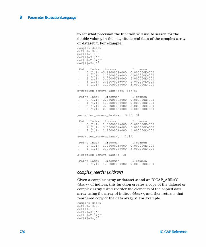
730
9 Parameter Extraction Language
to set what precision the function will use to search for the double value y in the magnitude real data of the complex array or dataset x. For example:complex def[5]def[0]=-3.23def[1]=1.000def[2]=3+j*5def[3]=2.3+j*1def[4]=3+j*5
!Point Index R:common I:common ! 0 (1,1) -3.230000E+000 0.000000E+000! 1 (1,1) 1.000000E+000 0.000000E+000! 2 (1,1) 3.000000E+000 5.000000E+000! 3 (1,1) 2.300000E+000 1.000000E+000! 4 (1,1) 3.000000E+000 5.000000E+000
x=complex_remove_last(def, 3+j*5)
!Point Index R:common I:common ! 0 (1,1) -3.230000E+000 0.000000E+000! 1 (1,1) 1.000000E+000 0.000000E+000! 2 (1,1) 3.000000E+000 5.000000E+000! 3 (1,1) 2.300000E+000 1.000000E+000
y=complex_remove_last(x, -3.23, 3)
!Point Index R:common I:common ! 0 (1,1) 1.000000E+000 0.000000E+000! 1 (1,1) 3.000000E+000 5.000000E+000! 2 (1,1) 2.300000E+000 1.000000E+000
z=complex_remove_last(y, "2.3")
!Point Index R:common I:common ! 0 (1,1) 1.000000E+000 0.000000E+000! 1 (1,1) 3.000000E+000 5.000000E+000
a=complex_remove_last(z, 3)
!Point Index R:common I:common ! 0 (1,1) 1.000000E+000 0.000000E+000
complex_reorder (x,idxarr)
Given a complex array or dataset x and an ICCAP_ARRAY idxarr of indices, this function creates a copy of the dataset or complex array x and reorder the elements of the copied data array using the array of indices idxarr, and then returns that reordered copy of the data array x. For example:complex def[5]def[0]=-3.23def[1]=1.000def[2]=3+j*5def[3]=2.3+j*1def[4]=3+j*5
IC-CAP Reference

Parameter Extraction Language 9
IC-CAP Reference
!Point Index R:common I:common ! 0 (1,1) -3.230000E+000 0.000000E+000! 1 (1,1) 1.000000E+000 0.000000E+000! 2 (1,1) 3.000000E+000 5.000000E+000! 3 (1,1) 2.300000E+000 1.000000E+000! 4 (1,1) 3.000000E+000 5.000000E+000
idxdef="ICCAP_ARRAY[5]"idxdef[0]=4idxdef[1]=3idxdef[2]=0idxdef[3]=2idxdef[4]=1
x=complex_reorder(def, idxdef)
!Point Index R:common I:common ! 0 (1,1) 3.000000E+000 5.000000E+000! 1 (1,1) 2.300000E+000 1.000000E+000! 2 (1,1) -3.230000E+000 0.000000E+000! 3 (1,1) 3.000000E+000 5.000000E+000! 4 (1,1) 1.000000E+000 0.000000E+000
complex_rsort (x,prec[,idxArr])
Given a complex array or dataset x, this function creates a copy of the dataset or complex array x, then sorts the elements in descending order, and then returns the sorted copy. The 2nd argument prec is used to specify the double precision to use when comparing elements during the sorting of the data array elements. The 3rd optional argument idxArr if specified, will be returned as an ICCAP_ARRAY of sorted integer indices. For example:complex def[5]def[0]=1.000def[1]=-3.23def[2]=3+j*5def[3]=2.3+j*1def[4]=3+j*5
!Point Index R:common I:common ! 0 (1,1) 1.000000E+000 0.000000E+000! 1 (1,1) -3.230000E+000 0.000000E+000! 2 (1,1) 3.000000E+000 5.000000E+000! 3 (1,1) 2.300000E+000 1.000000E+000! 4 (1,1) 3.000000E+000 5.000000E+000
x=complex_rsort(def,4)
!Point Index R:common I:common ! 0 (1,1) 3.000000E+000 5.000000E+000! 1 (1,1) 3.000000E+000 5.000000E+000! 2 (1,1) 2.300000E+000 1.000000E+000! 3 (1,1) 1.000000E+000 0.000000E+000! 4 (1,1) -3.230000E+000 0.000000E+000
731

732
9 Parameter Extraction Language
idxdef=""y=complex_rsort(def, 4, idxdef)
!Point Index R:common I:common ! 0 (1,1) 3.000000E+000 5.000000E+000! 1 (1,1) 3.000000E+000 5.000000E+000! 2 (1,1) 2.300000E+000 1.000000E+000! 3 (1,1) 1.000000E+000 0.000000E+000! 4 (1,1) -3.230000E+000 0.000000E+000
! idxdef = {2,4,3,0,1}
complex_sort (x,prec[,idxArr])
Given a complex array or dataset x, this function creates a copy of the dataset or complex array x, and sort the elements in ascending order, and then returns that sorted copy of the complex array or dataset x. The 2nd argument prec is used to specify the double precision to use when comparing elements during the sorting of the data array elements. The 3rd optional argument idxArr, if specified, will be returned as an ICCAP_ARRAY of sorted integer indices. For example:complex def[5]def[0]=1.000def[1]=-3.23def[2]=3+j*5def[3]=2.3+j*1def[4]=3+j*5
!Point Index R:common I:common ! 0 (1,1) 1.000000E+000 0.000000E+000! 1 (1,1) -3.230000E+000 0.000000E+000! 2 (1,1) 3.000000E+000 5.000000E+000! 3 (1,1) 2.300000E+000 1.000000E+000! 4 (1,1) 3.000000E+000 5.000000E+000
x=complex_sort(def,4)
!Point Index R:common I:common ! 0 (1,1) -3.230000E+000 0.000000E+000! 1 (1,1) 1.000000E+000 0.000000E+000! 2 (1,1) 2.300000E+000 1.000000E+000! 3 (1,1) 3.000000E+000 5.000000E+000! 4 (1,1) 3.000000E+000 5.000000E+000
idxdef=""y=complex_sort(def, 4, idxdef)
!Point Index R:common I:common ! 0 (1,1) -3.230000E+000 0.000000E+000! 1 (1,1) 1.000000E+000 0.000000E+000! 2 (1,1) 2.300000E+000 1.000000E+000! 3 (1,1) 3.000000E+000 5.000000E+000! 4 (1,1) 3.000000E+000 5.000000E+000
IC-CAP Reference

Parameter Extraction Language 9
IC-CAP Reference
! idxdef = {1, 0, 3, 2, 4}
cutstr(x,y[,delimiter])
Returns the size of ICCAP_ARRAY y. Divides a string x into substrings, saving the substrings in ICCAP_ARRAY y, using either whitespace substrings (tabs, spaces, newlines) or an explicitly passed 3rd argument as a delimiter. The leading space will be ignored when using the whitespace as a delimiter.x="a b c"print cutstr(x,y)! y = {"a", "b", "c"}
x="a b c"print cutstr(x,y)! y = {"a", "b", "c"}
x="a,b,c"print cutstr(x,y, ",")! y = {"a", "b", "c"}
x="a,,b,c"print cutstr(x,y, ",")! y = {"a", "", "b", "c"}
x="aspambspamc"print cutstr(x,y, "spam")! y = {"a", "b", "c"}
Output :33343
dataset
Enables you to access the dataset referred to by a string. A second argument may be specified which is a variable to receive any error string normally going to a red error box.
exp
e is raised to the power specified by the argument.
fix_path$
Guarantees a path appropriate for the current architecture.
733

734
9 Parameter Extraction Language
fix_path$(<path>)
Returns a string based on the passed in <path>, which is either a filename or a directory. The returned string will be the same filename or directory converted to the local architecture.
On UNIX, this converts Windows directory separators '\' to UNIX directory separators '/'. On the PC, it does the opposite and also takes care of any cygwin path dependencies.
Since IC-CAP uses the cygwin shell to execute the PEL system() and system$() commands, certain calls have cygwin dependencies. For example,print system$(“echo $HOME”)
may return something like /cygdrive/d/users/icuser, which does not have the Windows feel. Therefore, you may want to rewrite the PEL as follows:print fix_path$(system$(“echo $HOME”))
which returns d:\users\icuser using the above example.
get_user_region_names(x,y)
Returns the size of ICCAP_ARRAY y. Returns a list of names for the user defined regions of a plot (and a plot within a multiplot).x = get_user_region_names("<Object>", y)
For a multiplot, specify the plot number in brackets after the object:x = get_user_region_names("<Object>/Multiplot[1]", y)
imag
Extracts the imaginary part of a data set, matrix, or complex number.
imaginary
Extracts the imaginary part of a data set, matrix, or complex number.
IC-CAP Reference

Parameter Extraction Language 9
IC-CAP Reference
index_of(x,y,pos[,prec])
Returns the integer index of the first element found starting at position pos that has the same value as y in the ICCAP_ARRAY, dataset, or complex array x. If no elements are found in the data array x, then -1 is returned. The 2nd argument y can be a string or a double value. If value y is a double value, then the optional 4th argument prec can be used to set what precision the function will use to search for the element with the same double value y in the ICCAP_ARRAY, dataset, or complex array x. For example:abc="ICCAP_ARRAY[6]"abc[0]="foo"abc[1]=1.235abc[2]=2.33abc[3]="foo"abc[4]=3abc[5]=-10.23919
! abc = {"foo", 1.235, 2.33, "foo", 3, -10.23919}
print "ICCAP_ARRAY output:"print index_of(abc, "unknown", 0)print index_of(abc, 3, 0)print index_of(abc, 3, 5)print index_of(abc, -10.24, 0, 3)print index_of(abc, "foo", 0)print index_of(abc, "foo", 1)
complex def[5]def[0]=-3.23def[1]=1.000def[2]=3+j*5def[3]=2.3+j*1def[4]=3+j*5
!Point Index R:common I:common ! 0 (1,1) -3.230000E+000 0.000000E+000! 1 (1,1) 1.000000E+000 0.000000E+000! 2 (1,1) 3.000000E+000 5.000000E+000! 3 (1,1) 2.300000E+000 1.000000E+000! 4 (1,1) 3.000000E+000 5.000000E+000
print "Complex array output:"print index_of(def, "2.3", 4)print index_of(def, "2.3", 0)print index_of(def, 3, 0, 4)print index_of(def, 3, 3, 4)
Output:
ICCAP_ARRAY output:-14-15
735

736
9 Parameter Extraction Language
03
Complex array output:-1324
last_index_of(x,y[,prec])
Returns the integer index of the last element that has the same value as y in the ICCAP_ARRAY, dataset, or complex array x. If no elements are found in the data array x, then -1 is returned. The 2nd argument y can be a string or a double value. If value y is a double value, then the optional 3rd argument prec can be used to set what precision the function will use to search for the element with the same double value y in the ICCAP_ARRAY, dataset, or complex array x. For example:abc="ICCAP_ARRAY[6]"abc[0]="foo"abc[1]=1.235abc[2]=2.33abc[3]="foo"abc[4]=3abc[5]=-10.23919
! abc = {"foo", 1.235, 2.33, "foo", 3, -10.23919}
print "ICCAP_ARRAY output:"print last_index_of(abc, "unknown")print last_index_of(abc, 3)print last_index_of(abc, -10.24, 3)print last_index_of(abc, "foo")
complex def[5]def[0]=-3.23def[1]=1.000def[2]=3+j*5def[3]=2.3+j*1def[4]=3+j*5
!Point Index R:common I:common ! 0 (1,1) -3.230000E+000 0.000000E+000! 1 (1,1) 1.000000E+000 0.000000E+000! 2 (1,1) 3.000000E+000 5.000000E+000! 3 (1,1) 2.300000E+000 1.000000E+000! 4 (1,1) 3.000000E+000 5.000000E+000
print "Complex array output:"print last_index_of(def, 35.355, 4)print last_index_of(def, "2.3")print last_index_of(def, 3.0, 4)print last_index_of(def, "3.00")
Output:
IC-CAP Reference

Parameter Extraction Language 9
IC-CAP Reference
ICCAP_ARRAY output:-1453
Complex array output:-1344
log
Computes log base e.
log10 or lgt
Computes log base 10.
lookup_instr_table_val or lookup_instr_table_val_eval
Enables you to access the value of a field in an instrument options table. The first argument is the path to the table. The second argument is the field in the table (see “Set Table Field Value” on page 978 for syntax to specify the field name). An optional third argument may be specified which is a variable to receive any error string normally going to a red error box. lookup_instr_table_val returns NUMPTS if NUMPTS is a variable in # of Points. lookup_instr_table_val_eval returns 100 (presuming NUMPTS evaluates to 100).
lookup_obj_attribute
Enables you to access the state or attributes of a plot. The first argument is the object and the second argument is the keyword. The syntax is:X=lookup_obj_attribute("<Object>","Keyword")
For a Multiplot, specify the plot number in brackets after the object:X=lookup_obj_attribute("<Object>[N]", "Keyword")
For example:X=lookup_obj_attribute("/my_model/ my_dut/my_setup/my_multiplot/ Multiplot[1],"UserSelectedRegion")
737

738
9 Parameter Extraction Language
This example returns the coordinates of the white box that the user drew on the second plot (index=1) of the Multiplot my_multiplot.
The following table lists supported keywords.
Object Keyword Return Value
model POWindowOpen Int flag 0/1
plot POEnable Int flag 0/1
plot ErrorEnable Int flag 0/1
plot IsErrorRelative Int 1 is error is relative, 0 if error is absolute
plot ErrorRegion Data set array of 5 pointsX1,x2,y1,y2, color Color always returns 3 (green)
plot UserRegion/<Name> Data set array of 5 pointsX1,x2,y1,y2, color
plot PORegionNumber Number of Plot Optimizer regions
plot PORegion[N] Dataset array of 4 pointsX1,x2,y1,y2
plot UserSelectedRegion (white box)
Dataset array of 6 pointsReturns the coordinate of the white box:X1,x1,y1,y2,z1,z2Where z1,z2 are the coordinates with respect to the Y2 axis
plot UserSelectedPoint Dataset array of 4 points• selected point in the dataset• selected trace (0-8 with 8 being the
Y2 trace)• selected type:
0 (transform) 1(measured) 2 (simulated)
• selected curve
IC-CAP Reference

Parameter Extraction Language 9
IC-CAP Reference
lookup_par
Enables you to access the value of a parameter referenced by a string. A second argument may be specified which is a variable to receive any error string normally going to a red error box.
lookup_table_val or lookup_table_val_eval
Enables you to access the value of a field in an input, output, plot, parameter, or optimizer table. The first argument is the path to the table. The second argument is the field in the table (see “Set Table Field Value” on page 978 for syntax to specify the field name). An optional third argument may be specified which is a variable to receive any error string normally going to
plot NumHighlightedCurves Number of curves that were marked highlighted via PEL function: lookup_obj_attribute(plot_str&"/Trace[i]", "NumHighlightedCurves") ( i is the index of the trace that belong to the plot “plot_str”)
plot HighlightedCurveIndex The curve index of the highlighted curve that was marked highlighted via PEL function: lookup_obj_attribute(plot_str&"/Trace [i]/Hicurve[j]", "HighlightedCurveIndex") ( i is the index of the trace that belong to the plot plot_str, j is the index of the highlighted curve that belong to the trace plot_str&”/Trace[i]”)
plot GraphicMouseState Returns 2 if a white box is selected
plot XAxisDisplayType -1 (Unknown) 0 (Linear), 1(Log) or 2 (dB)
plot YAxisDisplayType -1 (Unknown) 0 (Linear), 1(Log) or 2 (dB)
plot Y2AxisDisplayType -1 (Unknown) 0 (Linear), 1(Log) or 2 (dB)
Multiplot only
SelectedPlot Returns selected plot
Object Keyword Return Value
739

740
9 Parameter Extraction Language
a red error box. lookup_table_val returns NUMPTS if NUMPTS is a variable in # of Points. lookup_table_val_eval returns 100 (presuming NUMPTS evaluates to 100).
lookup_var
Enables you to access the value of a variable referenced by a string. A second argument may be specified which is a variable to receive any error string normally going to a red error box.
lwc$(x)
Returns the lower case version of the string x. For example:print lwc$("Hello")
Output:
hello
mag or magnitude
Computes the magnitude for a complex number, or for each complex number in a matrix, data set, or data set of matrices.
max
Takes any number of arguments, as in HP BASIC. The argument list can be a mixture of scalars and data sets, and the function returns the maximum value found in any of them. This always returns a single real number, and only the real parts are considered. If matrices are received, only the 1,1 points are considered.
mdata(expr)
Returns the measured part of the argument expr.
min
Behaves like max, but returns the minimum value.
IC-CAP Reference

Parameter Extraction Language 9
IC-CAP Reference
ph or phase
Computes the phase angle in radians for a complex number, or for each complex number in a matrix, data set, or data set of matrices.
real
Extracts the real part of a data set, matrix, or complex number.
rowsof(x)
Returns an integer number of rows in a matrix, complex array of matrix data, or a data set x. For example:complex def[4]complex ghi.55[4]
print rowsof(def)print rowsof(ghi)
Output:
15
sdata(expr)
Returns the simulated part of the argument expr.
size
Returns the number of points in a data set, which is an integer.
sizeof(x)
Returns an integer number of elements in a variable ICCAP_ARRAY, or a complex array of data, or a data set. Returns 0 if x doesn't represent a data array or if the data array is empty or both. For example:abc="ICCAP_ARRAY[5]"abc[0]=1abc[1]=2abc[2]=3abc[3]=3abc[4]=12
complex def[4]def[0]=1.000def[1]=1+j*1
741

742
9 Parameter Extraction Language
def[2]=5def[3]=6
complex ghi.55[3]
x=1.354529
print sizeof(abc)print sizeof(def)print sizeof(ghi)print sizeof(x)
Output:
5
430
sqrt
Square root function. Complex and negative quantities produce correct complex or imaginary results.
strlen(x)
Returns the number of characters in the string x. For example:print strlen("Hello")
Output:
5
strpos(x,y)
Returns the index of the first occurrence of substring str2 found in string str1. An optional third argument may be specified which is an integer starting position that should be greater than or equal to 1. The starting position can be used to specify the starting index within the string str1 to start searching for substring str2. For example:print strpos("Hello","ell")print strpos("Hello","He")print strpos("Hello","dog")print strpos("Hello","l",1)print strpos("Hello","l",4)print strpos("Hello","l",5)
Output:210
IC-CAP Reference

Parameter Extraction Language 9
IC-CAP Reference
340
strrpos(str1,str2 [,endpos])
Returns the index of the last occurrence of substring str2 found in string str1. An optional third argument may be specified which is an integer end position that should be greater than or equal to 1. The end position can be used to specify the last index within the string str1 to search for the last occurrence of substring str2, using the search range of index 1 to endpos. For example:print strrpos("Hello","ell")print strrpos("Hello","He")print strrpos("Hello","dog")print strrpos("Hello","l",1)print strrpos("Hello","l",4)print strrpos("Hello","l",5)
Output:210044
substr$(x,start,stop)
Extracts the substring from the start index to the stop index from the string x. The value “1” refers to the first character in the string. If stop is omitted, substr$ returns the string from start to the end of the string. For example:x="Hello"print substr$(x,4)print substr$(x,2,4)
Output:loell
sys_path$
Guarantees a path appropriate for passing to the system$() or system() command.
743

744
9 Parameter Extraction Language
sys_path$(<path>)
Returns a string based on the passed in <path>, which is either a filename or a directory. The returned string will be the same filename or directory converted to the proper format for the system$() or system() function.
Since IC-CAP uses the cygwin shell to process the PEL system$ and system calls, PC style paths may not work properly when passed as arguments to system functions.
For example, if the user’s response toLINPUT “Enter a filename”,pathprint system$(“ls -al “ & path)
is:
foobar — the code functions properly.
/tmp/foobar — the code functions properly because IC-CAP insures /tmp and /var/tmp exist in the system call environment.
d:foobar — the code does not function properly.
However, the following rewriteLINPUT “Enter a filename”,pathprint system$(“ls -al “ & sys_path$(path))
insures that the system$() call actually sees /cygdrive/d/foobar even when the user types d:foobar.
system
Accepts a string argument, which is a shell command to invoke. You can employ all valid shell I/O redirection and other shell syntax within the string argument. It returns an integer, which is the exit status of the shell. If the shell command generates output, it is printed in the terminal window from which the IC-CAP program was started; refer to system$. On the PC, if a syntax error appears, turn on screen debug for additional information.
IC-CAP Reference

Parameter Extraction Language 9
IC-CAP Reference
system
Accepts a string argument, which is a shell command to invoke. You can employ all valid shell I/O redirection and other shell syntax within the string argument. It returns an integer, which is the exit status of the shell. If the shell command generates output, it is printed in the terminal window from which the IC-CAP program was started; refer to system$. On the PC, if a syntax error appears, turn on screen debug for additional information.
system$
Similar to system; it captures the command’s output, instead of letting it go to the terminal window. Instead of returning an integer, it returns the output that the shell command generated. For example:my_date$ = system$("date") ! get datecom$="echo "&my_date$&"|cut -c 5-7"month$ = system$(com$) ! substring 5-7
On the PC, if a syntax error appears, turn on screen debug for additional information.
trim$(x,chars)
Where x is a string and chars is a string containing characters to be trimmed from x. This function trims the unwanted characters from the beginning and end of the string. The parameter for chars is optional. If chars is omitted, the default is to remove spaces from the beginning and end of the string. For example:x=" stuff here "print trim$(x)y="////stuff here__//__//"print trim$(y)print trim$(y,"/_")
Output:stuff here////stuff here__//__//stiff here
745

746
9 Parameter Extraction Language
upc$(x)
Returns the string x with all upper case characters. For example:print upc$("Hello")
Output:HELLO
val
Generates a number, given a string representation of a simple (not expression) integer, floating point, or complex number. For example:linput "give a number",x$x = val(x$)
val$
Generates a string, given a numeric expression. In conjunction with the & operator (string concatenation), it can be useful for formatting. The optional second argument can either be an integer or a string.
• If no optional argument is given, the conversion uses the %g printf conversion (see printf() man page for details). The number is converted with WORKING_PRECISION digits of precision. If WORKING_PRECISION is not set, 6 digits are used.
• If the second argument is an integer, then the integer is interpreted as the number of digits of precision to use in a %g printf() conversion (see printf() man page for details).
• If the second argument is %nnICFMT where nn are optional integers, then the number is converted to a string according to IC-CAP default conversion routine, which uses unit multipliers (e.g., 1.23e-12 is converted to 1.23p). The optional nn specifies the number of digits of precision. If nn is less than 4, it is clamped to 4. If nn is omitted, then WORKING_PRECISION digits are used, if WORKING_PRECISION is not defined, 4 digits will be used.
IC-CAP Reference

Parameter Extraction Language 9
IC-CAP Reference
• If the second argument is any other string, it should contain exactly one of %e, %E, %g, %G, or %f. See the printf() man page for optional modifiers to these formats that specify the number of digits and spacing.
Examples:x=1.23456789e-12 print val$(x,"%ICFMT") ! 1.235p (Assuming WORKING_PRECISION not set) print val$(x,"%1ICFMT")! 1.235p (clamped to 4) print val$(x,"%8ICFMT") ! 1.2345679p (8 digits total) print val$(x,"abc %ICFMT") ! abc ICFMT (‘abc ’ on Linux) (uses printf syntax)print val$(x,"%e") ! 1.234568e-012 (printf format ignores WORKING_PRECISION)print val$(x,"%.3e") ! 1.235e-012 (specify 3 digits after decimal)print val$(x,"The number is %+12.4g.") !The number is +1.235e-012. (12 positions for entire number and +)print val$(x) ! 1.23457E-012 (6 digits of precision by default)print val$(x,7) ! 1.234568E-012
Built-In Constants
NOTE Real and complex scalars and data sets are accepted by all functions with the following exceptions: system, system$, and val expect to receive string data, and val$ expects a scalar number.
Several constants are recognized. Like statement names and built-in function names, these are reserved words (for example, you should not attempt to name a variable pi). The recognized constants are: PI or pi2PI or 2pi J or j (square root of -1)
747

9 Parameter Extraction Language
Expressions
748
As explained in the Data Types section, each type of data can be considered a simple expression. The primitive data types can make up more complex expressions by applying functions (such as log, or operators such as + ). In this section, expr denotes an expression; string_expr denotes a string expression.
(expr) expr + expr expr - expr expr * expr
Parentheses force precedence and group expressions.
expr / expr expr//expr
IC-CAP objects, including data sets, can be named using a slash (/). These same data sets can be used as arguments in a divide operation. To ensure the slash is understood as the divide operator, surround it with white space, or enter a double slash (//). If the slash is followed by a digit, divide is also understood, because a data set name in IC-CAP cannot start with a digit. The expression (ic)/(ib) is an example of another technique.
expr ^ expr expr ** expr
These operators express exponentiation, and are equivalents.
string_expr & string_expr
As in HP BASIC, this operator performs string concatenation.
log(expr) Performs a natural log function. For more information, refer to “Built-in Functions” on page 714 and “Calls to the Function Library” on page 752.
IC-CAP Reference

Parameter Extraction Language 9
IC-CAP Reference
To complete a computation, most operations make reasonable attempts to promote certain operands. For example, ib + 2e-6 promotes the scalar number 2e-6 to be a data set that, in turn, can be added to the data set ib.
For most arithmetic operations performed on a data set, the function or operator is applied point-by-point, producing a data set. The behavior of individual functions in this regard is clarified in their individual descriptions in “Built-in Functions” on page 714.
There are some limitations in the usage of the 5 basic arithmetic operators in working with data sets. For example:
• If ic is a data set, re-write 3//ic as 3*ic^ -1.
• The expression ic^ib is not supported when both operands are data sets.
• None of the binary operators * / + - ^ support an operation between a matrix and a data set.
The arithmetic in Programs is generally a complex floating point. Therefore, it is possible to see unexpected residue from integer or real arithmetic. For example: print (0+j)^2
may produce -1+j*1.22461E-16
rather than-1+j*0
This is due to finite precision in the library function that handles exponentiation of complex quantities.
Because complex arithmetic is used, success can occur where a function would be expected to fail in real arithmetic. For exampleacsh(.5)
yields 0+j*1.05
The complex arithmetic provides a wider domain of valid inputs, but in cases where a real input should produce a real output, the complex arithmetic is indistinguishable from real arithmetic.
749

9 Parameter Extraction Language
CAUTION Using the binary operators + and - (which have a higher precedence when used with the j notation) will produce unexpected results.
-1+j2 == -1-j*2(-1)+j2 == -1+j*2
750
Boolean Expressions
The expressions in this section can be used in the branching constructs (IF, IF...ENDIF, and WHILE...ENDWHILE), or can be used to generate the quantities 0 and 1. The abbreviation bool_expr denotes a boolean expression.
NOTE There is a distinction between the = operator (used for assignment) and the == operator. BASIC uses = for both assignment and comparison.
In some circumstances, == may not behave as expected. For example, if you repeatedly increment the quantity 0.3 by the amount 0.025, the results may be slightly less (in the 15th decimal place) than the expected sequence of values: 0.325, 0.350, ... , 0.4. Under these circumstances, == may yield FALSE unexpectedly. This is an inherent problem of expressing decimal numbers in binary floating point format.
expr == expr This operator tests for equality and can be used with string, integer, double, complex, and matrix types.
expr <> expr This operator tests for inequality and can be used with string, integer, double, complex, and matrix types.
expr > expr expr >= expr expr < expr expr <= expr
IC-CAP Reference
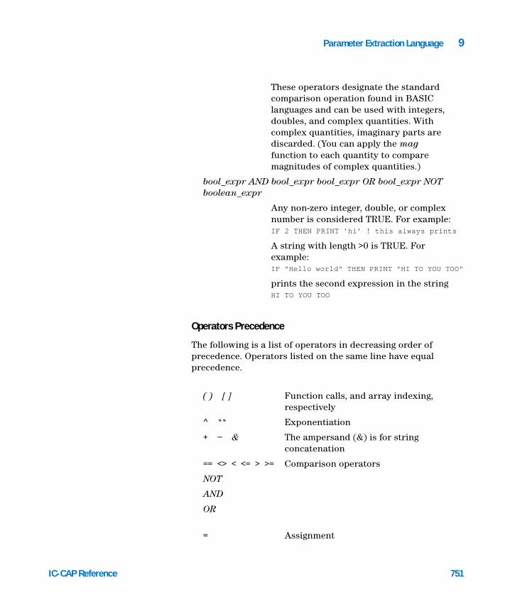
Parameter Extraction Language 9
IC-CAP Reference
Operators Precedence
The following is a list of operators in decreasing order of precedence. Operators listed on the same line have equal precedence.
These operators designate the standard comparison operation found in BASIC languages and can be used with integers, doubles, and complex quantities. With complex quantities, imaginary parts are discarded. (You can apply the mag function to each quantity to compare magnitudes of complex quantities.)
bool_expr AND bool_expr bool_expr OR bool_expr NOT boolean_expr
Any non-zero integer, double, or complex number is considered TRUE. For example: IF 2 THEN PRINT ’hi’ ! this always prints
A string with length >0 is TRUE. For example:IF "Hello world" THEN PRINT "HI TO YOU TOO"
prints the second expression in the stringHI TO YOU TOO
( ) [ ] Function calls, and array indexing, respectively
^ ** Exponentiation
+ − & The ampersand (&) is for string concatenation
== <> < <= > >= Comparison operators
NOT
AND
OR
= Assignment
751

752
9 Parameter Extraction Language
For example, it is TRUE that: -2^4 == -16
because the precedence of ^ exceeds that of − .
Calls to the Function Library
Any function in IC-CAP’s Function Browser can be called, such as sin, cos, and RMSerror. This greatly expands the availability of functions in expressions, Programs, and Macros. Some examples are:x = sin(pi/4) ! x takes on the value .707... x = linfit(ic,vc,0) ! x becomes a temporary data set with 2 pointsprint x[0] , x[1] ! slope and intercept are printed
To review the arguments used in a function, refer to Chapter 8, “IC-CAP Functions,” or create a stand-alone transform that uses the desired function and look at the resulting transform editor. For details on this procedure, refer to the section “Defining Transforms” in the User’s Guide. To call the library function in a Program, Macro, or table element, supply arguments in the same order shown in the editor.
The functions may expect some data set arguments, some real number arguments, and some strings or Model or DUT parameter names. Expressions can be used for the data set arguments and real number arguments. For the parameter names, use actual parameter names, IC-CAP system variable names, or quoted strings, string variables, or string expressions. If a function requires a string as a flag or switch of some sort, quote it. Otherwise the system thinks you are referring to an identifier such as a Model parameter, a system variable, or a temporary variable in a Program or Macro. The following example might clarify this point:! TwoPort requires strings as second and third arguments ! string argument dictates what type conversion to do x = TwoPort(S_out,"S","Y") ! this is OK x = TwoPort(S_out,S,Y) ! this is not, although... S = "S" ! initialize local variables S and Y Y = "Y" x = TwoPort(S_out,S,Y) ! now this is OK
IC-CAP Reference

Parameter Extraction Language 9
IC-CAP Reference
This point is mentioned because the quotation marks are not necessary if you use TwoPort as the function in a simple stand-alone Transform. The only other function that is like TwoPort in this regard is USERC_system, which requires a string to use as an operating system command.
Spell calls to functions contained in IC-CAP’s Function List must be spelled exactly as in the Function List.
The result from a call to a function in the library is usually a data set. For example:x = linfit(vc:log(ic.m),0)! get slope and intercept for log(ic.m)print x[0] ! print the slope of log(ic.m)
On the other hand, there are 2 cases in which the result of a library function is a single number or matrix, and not a data set. This makes library function calls more convenient, or usable within expressions in table elements. For example: x = sin(pi/4) ! x is now .70711 ...x = mean(ic.s) ! x is the average current value in ic.s
In the first example, sin is a function that can sometimes return a data set, if a data set is provided. In this example though, the input is a scalar number. Therefore, the system initializes x with a scalar number. A number of other functions behave like sin in this respect. They can be identified in the IC-CAP Functions List, because the Output of these functions is said to be a single number or an array, dependent on the Input Arguments.
In the second example, mean receives a data set as input. However, by definition it always produces a scalar, so x is initialized as a single number, and not a data set. A call to the variance, correlation, or RMSerror functions also produces a single number, and not a data set.
Some library functions, particularly extractions, yield null data sets; they do not appear to generate data, but they set parameters to new values.
753

754
9 Parameter Extraction Language
IC-CAP Reference

Agilent 85190A IC-CAP 2008Reference
10File Structure and Format
File Structure 756
This chapter describes the format of the IC-CAP .mdl file and associated files that can be written to and read from the system. When read into the system, these files restore IC-CAP to a previously saved state. Knowledge of the design of these files allows advanced users to perform many creative modifications to an IC-CAP configuration.
755Agilent Technologies

10 File Structure and Format
File Structure
756
All files used by IC-CAP are stored in an ASCII format that can be accessed by standard HP-UX tools and editors. IC-CAP Model files have a user-defined name; the extension is assigned by the system. The following table lists the file types and extensions.
The .mdl file is a combination of the file types listed below it. If all Models currently loaded are saved together, they are put in a single .mdl file. The complete Model file contains a circuit description, a model parameter set, Macros, and DUT descriptions. The DUT description in turn contains a DUT parameter set, a Test Circuit, and Setups. The Setups contain Inputs, Outputs, Transforms, and Plots.
The hardware description is global to IC-CAP and is not a part of a Model file. It can be saved in a .hdw file. It is also found in the .icconfig file in the user’s home directory. In
Table 73 IC-CAP File Types and Extensions
File Type Extension File Type Extension
Dataset .ds Data management .mdm
Hardware .hdw Setup .set
Model .mdl Input .inp
Circuit .cir Output .out
Model Parameters
.mps Transform .xfm
Macro .mac Plot .plt
DUT .dut Instrument Options .iot
DUT Parameters .dps Variables Table .vat
Test Circuit .tci Input .inp
Statistical data .sdf
IC-CAP Reference

File Structure and Format 10
IC-CAP Reference
addition to the hardware description, this file contains values of system variables, and status information for windows that are directly available from the Main Menu.
The individual major sections of the complete Model file begin with the word LINK followed by the type (for example, Model or DUT) and a name. The supporting information under this defines the appropriate configuration for IC-CAP. The hierarchy of related items in each file is defined by sets of braces { }. A major section title is followed by an open brace { and continues until the complementary closing brace }.
Within a section there are several key words that indicate the function of the associated information. When a single key word is on a line, the associated information is on the lines below. For some key words, their associated information is in fields to the right only, while for others, associated information is in fields to the right and lines below. These key words are summarized in the following table.
When editing an IC-CAP Model file, key words and braces must be in the correct locations for the file to be correctly read into IC-CAP. Editing the file with a text editor can be quite productive in some areas. When developing large Program Transforms or Macros, you may find it more convenient to create these with an editor outside of IC-CAP and read them in. When doing this, begin each line of text in your Program Transform or Macro with the pound sign (#).
Table 74 Key words in the IC-CAP File Structures
Key Word Definition
LINK major IC-CAP building block
applic application window that can be opened by IC-CAP
subapp title within an application
TABLE collection of user-modifiable elements
757

758
10 File Structure and Format
element user-programmable field (input box)
HYPTABLE table that is dynamically configured by IC-CAP
BLKEDIT block editor text follows (note: leading space in text)
CNTABLE connection table—not currently used in IC-CAP
PSTABLE parameter set table
param model parameter name and value
data configuration data follows belonging to the LINK item
dataset collection of numerical data
datasize dimensional information for a dataset
type MEASured, SIMUlated, or COMMON data points to follow
point individual data value—index, row, column, real value, imaginary value
list this item is dependent on the owning LINK item
member the owning LINK item is dependent on this item
Table 74 Key words in the IC-CAP File Structures (continued)
Key Word Definition
Example File
The following truncated Model file illustrates the structure described. Comments enclosed in angle brackets < > describe the file contents; they are not part of the actual IC-CAP file. Variable Tables or lines that start with applic or subapp are optional. It is not necessary for these lines to be present for a file to be successfully read by IC-CAP.
IC-CAP Reference

File Structure and Format 10
{ PSTABLE "Parameter Table" { } } } Link DAT "idvd" <DAT is internal name for Setup> { LINK MODEL "diode" <first line of an IC-CAP .mdl file> { applic "Edit" 1 83 194 <main model window is open & at pixels 83,194> subapp "dset_tile" 1 < DUT-Se tup tile is open>TABLE "Variable Table" <Variable Table for Model "diode"> { element 0 "Name" "SIMULATOR"element 0 "Value" "spice2" element 1 "Name" "" element 1 "Value" "" } LINK CIRC "Circuit" <circuit description starts here> { applic "Edit" 0 12 328 subapp "Circuit" 1 data { circuitdeck { D1 1 = A 2 = C DIODE <all lines in circuit have a leading space> .MODEL DIODE D + IS = 1E-14 + N = 1.0 } } } <circuit description ends here> Link PS "Parameter Set" { applic "Edit" 0 7 137 subapp "Parameter Table" 1data { PSTABLE "Parameter Table" { param IS 10.01f param N 999.7m } } } Link DUT "dc" { applic "Edit" 0 -1 -1 <DUT editor is closed, has not been opened yet> applic "Edit Variables" 0 -1 -1 subapp "setup_list" 1 Link TCIRC "Test Circuit" { subapp "Test Circuit" 0 data {
IC-CAP Reference 759

10 File Structure and Format
circuitdeck { } <end test circuit deck> } <end data section> } <end Test Circuit> Link DPS "Device Parameter Set" { subapp "Parameter Table" 1 data applic "Edit" 0 382 136 <Setup "idvd" is closed> applic "Instrument Options" 0 -1 -1 <instrument options table not opened yet> applic "Edit Variables" 0 -1 -1 <variables editor not opened yet> subapp "SWEEP" 1 subapp "OUT" 1 subapp "XFORM" 1 subapp "PLOT" 1 subapp "Instrument Table List" 1 subapp "Variable Table" 1 Link SWEEP "va" <Input sweep specification starts here> { applic "Display Data" 0 -1 -1 subapp "Edit Sweep Info" 1 subapp "Display Data" 1 data { HYPTABLE "Edit Sweep Info" <start of dynamic table definition> { element "Mode" "V" element "Sweep Type" "LIN" } HYPTABLE "Edit Sweep Mode Def" { element "+ Node" "A" element "- Node" "GROUND" element "Unit" "SMU1" element "Compliance" " 100.0m" } HYPTABLE "Edit Sweep Def" { element "Sweep Order" "1" element "Start" " 300.0m" element "Stop" " 1.000 " element "# of Points" "29" element "Step Size" " 25.00m" } } <end of dynamic table definition> list XFORM "extract" <Transform "extract" is dependent on this Input> list PLOT "i_vs_v" <Plot has similar dependency> } <Input specification "va" ends here> <repeat of similar Input not shown> Link OUT "ia" <Output specification starts here> { < file contents here similar to Input case & not shown>dataset <start of measured and simulated data> { datasize BOTH 29 1 1 <key: type #-of-points #-of-rows #-of-columns> type MEAS <measured data> <key: index row column real imaginary> point 0 1 1 1.09023e-09 0 <data point 0 has single value real number> point 1 1 1 2.86573e-09 0 <note: s-parameters would have 4 values per point> point 2 1 1 7.53339e-09 0 <corresponding to s11 s12 s21 and s22
760 IC-CAP Reference

File Structure and Format 10
point 3 1 1 1.98044e-08 0 <would be complex (real & imag) values> point 4 1 1 5.20644e-08 0 <other data points not shown> type SIMU <simulated data> point 0 1 1 1.09513e-09 0 point 1 1 1 2.87943e-09 0 <other data points not shown - same number as MEAS> } } list XFORM "optim_is_n" <Transform "optim_is_n" is dependent upon this Output> list PLOT "i_vs_v" <Plot has similar dependency> } Link XFORM "extract" <extraction Transform starts here> { data { HYPTABLE "Link Transform" { element "Function" "Program" } BLKEDIT "Program Body" <prog body starts here - note leading space> { ! Program Transform to extract IS, N, RS ! from forward diode I-V characteristics ! ! Note: print statements go to the ! window used to start IC-CAP
print "Example Program Transform to extract DC Diode Parameters"
index = 0 ! array index ! ! pick 2 low current points for IS & N ! to be extracted from
v1 = va[index] ! 1st voltage step WHILE v1 < 0.4 ! get first data
index = index + 1 ! point pair v1 = va[index]
END WHILE i1 = ia[index]
< more program exists but is not shown> print "... end of program Transform extraction ..."
} dataset { datasize COMMON 29 1 1 <key: type #-of-points #-of-rows #-of-columns> type COMMON <COMMON specification means that the same data is > point 0 1 1 0 0 <used to represent measured & simulated data. > point 1 1 1 0 0 <However, the data space is not used by this > point 2 1 1 0 0 <transform, which calculates parameter values only>
<more points not shown> }}member SWEEP "va" <this Transform is dependent on Input "va"> member OUT "ia" <this Transform is dependent on Output "ia"> }
IC-CAP Reference 761

10 File Structure and Format
Link PLOT "i_vs_v" <Plot definition starts here> { applic "Display Plot" 0 5 435 <Plot window is closed, but located at pixels 5,435> applic "Display Data" 0 -1 -1 <data window has never been opened> subapp "Edit plot Info" 0 subapp "Display Data" 1 data { plotsize 11960 8970 <Plot size is 11960x8970 (in 1/100 mm)> HYPTABLE "Edit plot Info" { element "Report Type" "XY GRAPH" } HYPTABLE "Edit Plot Def" { element "X Data" "va" element "Y Data 0" "ia" element "Y Data 1" "" element "Y Data 2" "" element "Y Data 3" "" element "Y Data 4" "" element "Header" "" element "Footer" "" element "X Axis Type" "LINEAR" element "Y Axis Type" "LINEAR" element "Y2 Axis Type" "LINEAR" element "Y2 Data" "" } } member INPUT "va" member OUT "ia" } data <data section for Setup - instrument options table information> { TABLE "HP4141.7.23" <HP4141 DC parameter measurement instrument> { element 0 "Use User Sweep" "No" element 0 "Hold Time[0-650s]" " 0.000 " element 0 "Delay Time[0-6.5s]" " 0.000 " element 0 "Integ Time" "S" } TABLE "HP4275.7.10" { element 0 "Hold Time[0-650]" " 0.000 " element 0 "Delay Time[0-650]" " 0.000 " element 0 "High Res" "No" element 0 "Meas Freq (KHz)" "10" } } } } } <end of complete Model file>
762 IC-CAP Reference

Agilent 85190A IC-CAP 2008Reference
11Variables
Several variable names are reserved by IC-CAP and cannot be used for user-defined variables. You can assign values to reserved variables and define your own variables at several different levels:
• Globally
• Model
• DUT
• Setup
These levels can be viewed as a hierarchy where variables at lower levels inherit their values from variables at some level above them.
You define global variables through the IC-CAP/Main window. These variables apply to all Models, DUTs, and Setups unless you explicitly set the variables differently at the Model, DUT, or Setup level.
You define Model, DUT, and Setup variables through the Model window:
• Model variables apply to all DUTs and Setups of that Model unless you explicitly set the variables differently for individual DUTs and/or Setups.
• DUT variables apply to all Setups of that DUT unless you explicitly set the variables differently for individual Setups.
• Setup variables apply only to that Setup.
763Agilent Technologies

11 Variables
CAUTION The maximum string length for a variable table is 15 K characters. Exceeding this limit may cause a core file to be generated when saving or reading a file.
764
Table 75 Plot Characteristics
Variable Description
ANNOTATE_AUTO Sets a flag to enable or disable automatic annotation update upon data changes. Default is No.
ANNOTATE_CSET Sets a Starbase character set to be used for annotation texts. Default value is determined by /usr/lib/starbase/defaults.
ANNOTATE_FILE Sets a file name from which a plot reads in an annotation text. Default is no file to read.
ANNOTATE_MACRO Sets a macro name that is executed by a Plot for generating an annotation text. Default is no macro to execute.
ANNOTATE_PLOTS Obsolete in IC-CAP 2006. Now to enable or disable annotation on a plot, use the Plot Options dialog box. See “Setting Plot Options” in the User’s Guide.
CDF_ERROR_FIT Can be set to TRUE or FALSE. TRUE will draw the Gaussian curve fitted to the Cumulative plot. Default is TRUE.
CHECK_PLOT_MATCH Lets IC-CAP check if a given XY pair belongs to the same Setup. If No, potentially mismatched XY pair can be shown in a tabular format with Display Data. Default is Yes.
DASH_DOT Sets the number of data points at which a simulated line changes from a dashed to a dotted line. Used in Plot. Default value is 32.
DYNAMIC_MULTIPLOT_MODE Sets the location where the manual scaling setting is saved for a Multiplot. If set to FALSE, the manual scaling setting for each subplot in a Multiplot is saved with the Multiplot, allowing different scaling to be saved for the same plot if opened as a single plot or on one or more Multiplot. If set to TRUE, the manual scaling setting for each subplot in a Mulitplot is saved with the subplot. In this mode, no matter where the plot is opened (as a single plot or on one or more Multiplots), it will use the same scaling information. However, if the same subplot appears on multiple Multiplots, or in multiple positions of the same Multiplot, then the settings for only the last subplot closed is saved. Default is FALSE.
IC-CAP Reference
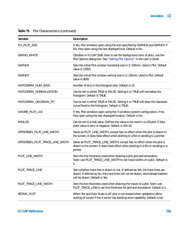
Variables 11
FIX_PLOT_SIZE If Yes, Plot windows open using the size specified by GWINDX and GWINDY. If No, they open using the last displayed size. Default is No.
GWIND_WHITE Obsolete in IC-CAP 2006. Now to set the background color of plots, use the Plot Options dialog box. See “Setting Plot Options” in the User’s Guide.
GWINDX Sets the initial Plot window horizontal size in 1/100mm. Used in Plot. Default value is 12500.
GWINDY Sets the initial Plot window vertical size in 1/100mm. Used in Plot. Default value is 9000.
HISTOGRAM_NUM_BINS Number of bins in the histogram plot. Default is 10.
HISTOGRAM_NORMALIZATION Can be set to either TRUE or FALSE. Setting it to TRUE will normalize the histogram. Default is TRUE.
HISTOGRAM_GAUSSIAN_FIT Can be set to either TRUE or FALSE. Setting it to TRUE will draw the Gaussian curve fitted to the histogram. Default is TRUE.
IGNORE_PLOT_LOC If Yes, Plot windows open using the X windows system configuration. If No, they open using the last displayed location. Default is No.
MINLOG Can be set to a real value. Defines the value to be used in a LOG plot, if data point value is zero or negative. Default is 10e-18.
OFFSCREEN_PLOT_LINE_WIDTH Same as PLOT_LINE_WIDTH, except has no effect when the plot is drawn to the screen. It does have effect when plotting to a file or sending to a printer.
OFFSCREEN_PLOT_TRACE_LINE_WIDTH Same as PLOT_TRACE_LINE_WIDTH, except has no effect when the plot is drawn to the screen. It does have effect when plotting to a file or sending to a printer.
PLOT_LINE_WIDTH Sets the line thickness used when drawing a plot grid and annotation. Note: use PLOT_TRACE_LINE_WIDTH to set trace widths on a plot. Default is 1.
PLOT_TRACE_LINE Sets whether trace line is drawn or not. If defined as Yes, the trace lines are drawn. If defined as No, the trace lines will not be drawn, and instead markers will be drawn. Default is Yes.
PLOT_TRACE_LINE_WIDTH Sets the line thickness used when drawing the traces of a plot. Note: use PLOT_TRACE_LINE to set line thickness for grid and annotation. Default is 1.
RETAIN_PLOT When Yes and Auto Scale is off, plot is not erased when updated to allow overlay of curves if the X server has backing store capability. Default is No.
Table 75 Plot Characteristics (continued)
Variable Description
IC-CAP Reference 765

11 Variables
RI_GRAPH_SYMMETRY When defined as Yes, the plot title is displayed. If defined as No, the plot title is not displayed. Default is Yes.
SCATTER_CONTOURS Can be set to either TRUE or FALSE. Setting it to TRUE will draw the contours. Default is TRUE.
SCATTER_NUM_SEGMENTS The number of segments with which to draw the contours. Default is 1500.
SHOW_GRID When No, plot eliminates XY grids and leaves tics. Default is Yes.
SHOW_PLOT_TITLE Obsolete in IC-CAP 2006. Now to show or hide the plot title, use the Plot Options dialog box. See “Setting Plot Options” in the User’s Guide.
USE_PLOT_LOOKUP Lets IC-CAP perform auto-lookup of X data from each Y data. Another way to disable auto-lookup is to use an arbitrary expression for an X data. Default is Yes.
Table 76 Plot Optimizer
Variable Description
AUTOSET_COEFF Sets the coefficient value used to calculate the Plot Optimizer's Min and Max parameter values. Min and Max parameter values are calculated as follows:if (value > 0) Min = value/coeff Max = value × coeffif (value < 0) Min = value × coeff Max = value/coeffif (value ==0) Min = -coeff Max = +coeffDefault is 5.
OPT_PARTABLE_SHOW_MODEL_ONLY If set to Yes, displays the model parameters in the parameter list shown in the parameter table tab of Plot Optimizer and normal Optimizer transforms. If set to No, displays all the model and DUT parameters found in the enable plots paths. Default is Yes for the Plot Optimizer and No for the Extract/Optimize folder.
Table 75 Plot Characteristics (continued)
Variable Description
766 IC-CAP Reference

Variables 11
OPT_PARTABLE_SHOW_PARS If set to Yes, displays all parameters, except model parameters, in the parameter list in the Plot Optimizer and Extract/Optimize folder. If set to No, hides the parameters. Default is Yes.
OPT_PARTABLE_SHOW_VARS If set to Yes, displays all variables in the parameter list in the Plot Optimizer and Extract/Optimize folder. If set to No, hides the variables. Default is Yes.
PLOTOPT_USE_YAXES_TYPE Sets whether the Plot Optimizer algorithm can use the LOG10() and DB() functions to insert the trace equations into the Plot Optimizer. If defined as Yes (Default), the Plot Optimizer algorithm uses the LOG10() function when the Y Axis Type is LOG10 and the DB() function when the Y Axis Type is DB.If defined as No, the Plot Optimizer algorithm does not use the LOG10() and DB() functions regardless of the Axis Type.Default is Yes.
PLOTOPT_AUTOCONFIG_WARNING Sets whether autoconfigure issues a warning to the Status window when one or more traces could not be autoconfigured. If defined as Yes (Default), a warning is issued when one or more traces could not be autoconfigured.If defined as No, no warning is issued when autoconfigure fails.Default is Yes.
Table 77 Calibration
Variable Description
CAL_OPEN_C Obsoleted and replaced by CAL_OPEN_C0.
CAL_OPEN_C0 CAL_OPEN_C1 CAL_OPEN_C2
Sets the open capacitance of an Open standard in farads that is used with Software Calibration. The combined value Copen applies to both port 1 and 2. A second-order polynomial represents its frequency dependence. Default value is 0. Copen = C0 + C1 * F + C2 * F^2
CAL_Z0 Obsoleted and replaced by TWOPORT_Z0.
Table 76 Plot Optimizer (continued)
Variable Description
IC-CAP Reference 767

768
11 Variables
Table 78 UI Options
Variable Description
DUT_TREE_COLS Controls the width of the tree list in the DUTs-Setups folder. The variable controls the folder in the scope of the variable table where it is defined. The variable’s value sets the list’s width in number of columns.
MACRO_LIST_COLS Controls the width of the Select Macro list in the Macros folder. The variable controls the folder in the scope of the variable table where it is defined. The variable’s value sets the list’s width in number of columns.
MAXIMUM_LIST_LENGTH The maximum number of value fields allowed for an input where LIST is the Sweep Type and a variable is used to specify ‘# of Values.’ If a constant is used to specify ‘# of Values,’ MAXIMUM_LIST_LENGTH is ignored. Default is 15.
MEAS_SIM_LIST_COLS Controls the width of the Input/Output Finder list in the Measure/Simulate folder. The variable, SHOW_INPUT_OUTPUT_FINDER, must be enabled to control the list width. The variable controls the folder in the scope of the variable table where it is defined. The variable’s value sets the list’s width in number of columns.
PARAMETER_PRECISION Specifies the number of digits used when displaying parameter values in the Parameters table and when sending the values to a simulator. Default is 4.
PLOT_LIST_COLS Controls the width of the Plot Finder list in the Plots folder. The variable controls the folder in the scope of the variable table where it is defined. The variable’s value sets the list’s width in number of columns.
RETAIN_DATA When Yes, data from a Setup is retained if a sweep limit changes but the number of points remains the same. Default is No, which causes the data to be zeroed.
RETAIN_SIMU A simulator run in piped mode is normally stopped if a new simulator is selected. If Yes, the old simulator is kept running, which will speed up simulations if there is frequent switching between simulators. Default is No.
SHOW_INPUT_OUTPUT_FINDER When Yes, enables the Input/Output Finder list in the Measure/Simulate folder. If you enable this variable or change its value after viewing the folder, you must close, then re-open the model for the change to take effect. Default is No.
IC-CAP Reference

Variables 11
WORKING_PRECISION Controls the precision of numeric values when converted to text. This precision setting affects only those parts of a model for which the variable is defined. Although all math in IC-CAP is performed using double precision, precision may be lost when a number is converted to text. This conversion occurs in the following situations: any time the function val$() is called; the PRINT statement is used; a numeric value is assigned to a variable in the IC-CAP Variable Table. Because all variables in the IC-CAP Variable Table are text by definition, assigning a numeric value to such a variable will implicitly call val$().
Range of values: 6 through 29. Default is 6.
Note: While settings above 17 are allowed, they seldom show any affect.
XFORM_LIST_COLS Controls the width of the Select Transform list in the Extract/Optimize folder. The variable controls the folder in the scope of the variable table where it is defined. The variable’s value sets the list’s width in number of columns
GUI_PAGE_SUPRESS_SUMMARY Normally, IC-CAP displays a short summary of each GUI Item on the GUI Items pages.To suppress this summary and display only the item name (for a cleaner look to the page), set this variable to anything but 0, F, FALSE, N, NO, or blank.
Table 79 PEL
Variable Description
ICCAP_MAXIMUM_CALL_CHAIN Sets the maximum number of transforms/macros (written in PEL) that can be
called (via iccap_func()) without returning. This limit may be set to protect
automations under development from infinitely recurring by accident. Without
this limit, such infinite recursions will cause IC-CAP to consume all the
memory available in your system and then crash. The default value is 0 which
means to permit any number of calls.
Table 78 UI Options (continued)
Variable Description
IC-CAP Reference 769
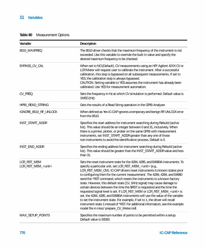
11 Variables
Table 80 Measurement Options
Variable Description
8510_MAXFREQ The 8510 driver checks that the maximum frequency of the instrument is not exceeded. Use this variable to override the built-in value and specify the desired maximum frequency to be checked.
BYPASS_CV_CAL When set to NO (Default), CV measurements using an HP/Agilent 42XX CV or LCR Meter will request user to calibrate the instrument. After a successful calibration, this step is bypassed on all subsequent measurements. If set to YES, the calibration step is always bypassed.CAUTION: Setting variable to YES assumes the instrument has already been calibrated. Use YES for measurement automation.
CV_FREQ Sets the frequency in Hz at which CV simulation is performed. Default value is 1MEG (Hz).
HPIB_READ_STRING Gets the results of a Read String operation in the GPIB Analyzer.
IGNORE_8510_RF_UNLOCK When defined as Yes IC-CAP ignores a temporary and benign RF UNLOCK error from the 8510.
INST_START_ADDR Specifies the start address for instrument searching during Rebuild (active list). This value should be an integer between 0 and 31, inclusively. When there is a printer, plotter, or prober on the same GPIB with measurement instruments, set INST_START_ADDR greater than any one of those non-instruments to avoid the identification process. Default is 0.
INST_END_ADDR Specifies the ending address for instrument searching during Rebuild (active list). This value should be greater than the INST_START_ADDR value and less than 31.
LCR_RST_MEMLCR_RST_MEM_<unit>
Sets the reset instrument state for the 4284, 4285, and E4980A instruments. To specify a particular unit, set LCR_RST_MEM_<unit> (e.g., LCR_RST_MEM_CM). IC-CAP drivers reset instruments to known states prior to configuring them for the current measurement. The 4284, 4284, and E4980 send the *RST command, which resets the instruments to a known factory state. However, this default state (1V, 1KHz signal) may cause damage to certain devices between the time the $RST is requested and the time the requested signal level is set. If LCR_RST_MEM or LCR_RST_MEM_<unit> is set, the 4284, 4285, and E4980A instruments will use the value of the variable to set the instrument state. For example, if set to 1, the driver will recall instrument state 1 instead of *RST. For additional information, see the example model file in misc/prepare_CV_Meter.mdl.
MAX_SETUP_POINTS Specifies the maximum number of points to be permitted within a setup. Default value is 50000.
770 IC-CAP Reference

Variables 11
MDS_MEASURE_FAST Flag reserved for use by the HPRoot model extraction in the High-Frequency IC-CAP software. Default is No.
MEASURE_FAST When Yes, IC-CAP will attempt to minimize instrument re-initialization during repeated measurements on the same Setup. Refer to Speeding Up Repetitive Measurements in the Measurement chapter. Default is No.
NO_ZEROING When Yes, IC-CAP will avoid a preliminary step of zeroing DC and other signal sources at the beginning of measurements. Refer to MEASURE_FAST. Default is No.
PARALLEL_INPUT_UNITS_OK Overrides a warning when multiple units share a single input node. Default value is No, to issue a warning.
PRE_5_8510_FIRMWARE For HP 8510B Network Analyzers with firmware revisions prior to HP8510B.05.00: Dec 5, 1988 only.
Declaring this variable prevents certain commands (DETENORB--set detector to normal bandwidth, and EXTTOFF--external triggr off) from being sent to the NWA. These commands are not supported in the above-referenced firmware and sending such commands causes a measurement failure. Declare this variable to prevent the failure.
No value assignment required.
8510_MAXFREQ The 8510 driver checks that the maximum frequency of the instrument is not exceeded. Use this variable to override the built-in value and specify desired maximum frequency to be checked.
Table 80 Measurement Options (continued)
Variable Description
IC-CAP Reference
ptions
Table 81 HP85124 Measurement OVariable Description
These variables are used to modify the source tuning process. Source tuning is specified with an entry in the options table. Source tuning process varies the supply voltage to compensate for I*R drop in getting to the device under test.
p1_step_size Type = REAL, Default = 0.0This variable sets a fixed step size for newton iterations when tuning the source voltage for port 1. Default is an auto step size, determined from dvm noise floor.
771

11 Variables
p2_step_size Type = REAL, Default = 0.0This variable sets a fixed step size for newton iterations when tuning the source voltage for port 2. Default is an auto step size, determined from dvm noise floor.
p1_step_scale Type = REAL, Default = 1.0This variable sets a scale factor to modify the auto step size in newton iterations when tuning the source voltage for port 1. The auto step size is multiplied by this value.
p2_step_scale Type = REAL, Default = 1.0This variable sets a scale factor to modify the auto step size in newton iterations when tuning the source voltage for port 2. The auto step size is multiplied by this value.
p1_tune_error Type = REAL, Default = 0.0This variable sets a fixed error goal for tuning the source voltage for port 1 instead of the default auto ranged error which is determined from the dvm noise floor.
p2_tune_error Type = REAL, Default = 0.0This variable sets a fixed error goal for tuning the source voltage for port 2 instead of the default auto ranged error which is determined from the dvm noise floor.
p1_error_scale Type = REAL, Default = 1.0This variable sets a scale factor to modify the auto ranged error goal for tuning the source voltage for port 1 The auto ranged error goal is multiplied by this value.
p2_error_scale Type = REAL, Default = 1.0This variable sets a scale factor to modify the auto ranged error goal for tuning the source voltage for port 2 The auto ranged error goal is multiplied by this value.
max_newton_iters Type = INT, Default = 6This variable sets the maximum number of newton iterations to complete before quitting the source tuning process.
pulse_rise_time Type = REAL, Default = 0.2E-6This variable specifies the average rise time for the pulse. This is used in determining if the measurement delay results in a measurement in the pulse. If the measurement for source tuning is not in the pulse then the resulting voltage will be very high.
pulse_fall_time Type = REAL, Default = 0.2E-6This variable specifies the average fall time for the pulse. This is used in determining if the measurement delay results in a measurement in the pulse. If the measurement for source tuning is not in the pulse then the resulting voltage will be very high.
These variables can be used to initiate printing of data to the status window. This data is useful in troubleshooting measurement problems and data accuracy questions.
Table 81 HP85124 Measurement Options
Variable Description
772 IC-CAP Reference

Variables 11
show_tuning Type = INT, Default = 0, Values 0 or 1When set to 1 measured values, tuning error, and next value to be tries are displayed for the source tuning process. These values are printed the status window.
show_samples Type = INT, Default = 0, Values 0 or 1When set to 1 all the dvm or adc measurements are displayed in the status window.
show_stats Type = INT, Default = 0, Values 0 or 1When set to 1 statistical information about the measured data is displayed. Data includes mean , min, and max. Data is displayed in the status window.
show_current_range Type = INT, Default = 0, Values 0 or 1When set to 1 the present current range is displayed to the status window when the measurement begins and any time the range changes.
show_voltage_range Type = INT, Default = 0, Values 0 or 1When set to 1 the present voltage range is displayed to the status window when the measurement begins and any time the range changes.
These variables are used to over-ride the offsets defined in the hp85124.cal file.
p1_meas_offset Type = REAL, Default = value in hp85124.calThis variable will over-ride the input_measurement_offset variable in the hp85124.cal file. This variable adjusts the delay for the port 1 voltage measurement.
p2_meas_offset Type = REAL, Default = value in hp85124.calThis variable will over-ride the output_measurement_offset variable in the hp85124.cal file. This variable adjusts the delay for the port 2 voltage measurement.
p1_meas_i_offset Type = REAL, Default = value in hp85124.calThis variable will over-ride the input_current_measurement_offset variable in the hp85124.cal file. This variable adjusts the delay for the port 1 current measurement. This offset is relative the voltage measurement.
p2_meas_i_offset Type = REAL, Default = value in hp85124.calThis variable will over-ride the output_current_measurement_offset variable in the hp85124.cal file. This variable adjusts the delay for the port 2 current measurement. This offset is relative the voltage measurement.
These variables are used to over-ride the instrument types specified in the hp85124.cfg file.
p1_v_type Type = STRING, Default = value in hp85124.cfgThis variable over-rides the value of dmm_vin in the hp85124.cfg file. This will also over-ride the automatic change for risetime mode. The default is to use the hp3458 dvm for slow mode and the internal adc (K49 only) for fast mode.
Table 81 HP85124 Measurement Options
Variable Description
IC-CAP Reference 773

11 Variables
p1_i_type Type = STRING, Default = value in hp85124.cfgThis variable over-rides the value of dmm_iin in the hp85124.cfg file. This will also over-ride the automatic change for risetime mode. The default is to use the hp3458 dvm for slow mode and the internal adc (K49 only) for fast mode.
p2_v_type Type = STRING, Default = value in hp85124.cfgThis variable over-rides the value of dmm_vout in the hp85124.cfg file. This will also over-ride the automatic change for risetime mode. The default is to use the hp3458 dvm for slow mode and the internal adc (K49 only) for fast mode.
p2_i_type Type = STRING, Default = value in hp85124.cfgThis variable over-rides the value of dmm_iout in the hp85124.cfg file. This will also over-ride the automatic change for risetime mode. The default is to use the hp3458 dvm for slow mode and the internal adc (K49 only) for fast mode.
These variables are used to make changes in the default settings used for the hp3458 dmms
dvm_terminals Type = CHAR, Default = R, Values = R or FThis variable will change which set of terminals the dmm will read. The choice is R for rear and F for front.
dvm_trigger_mode Type = CHAR, Default = E, Values = E or IThis variable will change the trigger mode of the dmm. E for external and I for internal.
dvm_aperture Type = REAL, Default = 1E-6This variable changes the value of the aperture for DCV mode of the dmms.
dvm_track_hold Type = INT, Default = 1, Values 0 or 1This variable sets either track and hold mode (DSDC) or integrated mode (DCV).
dvm_auto_zero Type = STRING, Default = ONCE, Values = OFF, ON, or ONCEThis variable sets the auto zero mode on the dmms.
allow_internal Type = INT , Default = 0, Values = 1/0This variable allows the dmm to take more samplings within the same pulse during time domain pulse profile measurements if the time interval is less than 20us.
Table 81 HP85124 Measurement Options
Variable Description
774 IC-CAP Reference

Variables 11
IC-CAP Reference
s
Table 82 General Extraction Option
Variable Description
EXTR_DUT Used internally in extractions. When a circuit or test circuit has been defined, set this variable to the name of the DUT whose parameters are either extracted or used by the IC-CAP device extraction functions.
EXTR_MODEL Used internally in extractions. When a circuit has been defined, set this variable to the name of the model whose parameters are either extracted or used by the IC-CAP device extraction functions.
POLARITY Specifies the device polarity of the device to be extracted. Allowed values for bipolar devices are NPN or PNP. Default is NPN for bipolar devices. Allowed values for MOS devices are NMOS or PMOS. Default is NMOS for MOS devices.
WORKING_PRECISION Controls the precision of numeric values when converted to text. This precision setting affects only those parts of a model for which the variable is defined. (Converting to text is done when: the function val$() is called; the PRINT statement is used; a numeric value is assigned to a variable in the IC-CAP Variable Table.) Range of values: 6 and higher. Default is 6.
Note: While settings above 17 are allowed, a double precision number cannot be expressed to this precision.
s
Table 83 General Simulation OptionVariable Description
DEFAULT_SIMU Sets the default simulator name. Used in Utilities.
MAX_DC_SWEEPS Specifies the maximum number of DC sweeps for a simulation. Default is simulator-dependent.
MAX_SETUP_POINTS Specifies the maximum number of points to be permitted within a setup. Default value is 50000.
OPEN_RES Specifies the resistance value that is automatically connected to all floating nodes in the circuit. This is available for all simulators with links to IC-CAP. When this variable is not specified, a zero amp current source is connected to the node.
PARAMETER_PRECISION Specifies the number of digits used when displaying parameter values in the Parameters table and when sending the values to a simulator. Default is 4.
775

11 Variables
SIMULATOR Specifies the simulator name to be used in all simulations performed under the level in which this variable is defined. The name must be a valid simulator; otherwise, the currently selected simulator is used. Default is the currently selected simulator.
SIM_USE_UPPER_CASE_PARAMS By default parameters are entered into the Parameters table with the same capitalization as entered in the circuit page. (The hpeesofsim simulator is an exception.) If set to 'F', 'N', 'FALSE','No' or '0' the default behavior will result. Any other setting will force the parameters in the Parameters table to be represented in upper case according to the following rules: • If the parameter was declared with $dpar, $mpar, or $xpar, capitalization is
not affected.• If the parameter contains a period, only the part of the parameter after the
last period is upper case.• If the parameter does not contain a period, the entire parameter is upper
case.If USE_OLD_CASE_PARM_RULE is set to anything other than 'F', 'N', 'FALSE','No' or '0' (case insensitive), this setting follows different rules. See USE_OLD_CASE_PARM_RULE.This setting affects all simulators but may be overridden by HPEESOFSIM_USE_LOWER_CASE_PARAMS and HPEESOFSIM_USE_MIXED_CASE_PARAMS for the hpeesofsim simulator.
SIM_USE_LOWER_CASE_PARAMS By default parameters are entered into the Parameters table with the same capitalization as entered in the circuit page. (The hpeesofsim simulator is an exception.) If set to 'F', 'N', 'FALSE','No' or '0' the default behavior will result. Any other setting will force the parameters in the Parameters table to be represented in lower case according to the following rules: • If the parameter was declared with $dpar, $mpar, or $xpar, capitalization is
not affected.• If the parameter contains a period, only the part of the parameter after the
last period is lower case.• If the parameter does not contain a period, the entire parameter is lower
case.If USE_OLD_CASE_PARM_RULE is set to anything other than 'F', 'N', 'FALSE','No' or '0' (case insensitive), this setting follows different rules. See USE_OLD_CASE_PARM_RULE.This setting affects all simulators but may be overridden by HPEESOFSIM_USE_LOWER_CASE_PARAMS and HPEESOFSIM_USE_MIXED_CASE_PARAMS for the hpeesofsim simulator.
Table 83 General Simulation Options (continued)
Variable Description
776 IC-CAP Reference

Variables 11
TEMP Temperature at which simulations are performed. When performing an optimization to extract model parameters, TEMP and TNOM should be set to the same value so that simulations during optimization are performed at TNOM. Default value is simulator-dependent.
TNOM Temperature at which the model parameters are extracted. TNOM must be defined in order to guarantee consistency between simulation and extraction. Default value is 27 when performing an extraction, and is simulator dependent when performing a simulation.
TWOPORT_C Sets a DC decouple capacitance value when a 2-port circuit is generated from a circuit for 2-port simulation. Default is 100 farad.
TWOPORT_L Sets an AC decouple inductance value when a 2-port circuit is generated from a circuit for 2-port simulation. Default is 100 henry.
TWOPORT_Z0 Sets a characteristic impedance value for 2-port circuit that is used in AC extractions, TwoPort function, and Software calibration. Default is 50 ohm.
USE_OLD_CASE_PARM_RULE If set to anything other than 'F', 'N', 'FALSE','No' or '0' (case insensitive), this setting changes the rules for SIM_USE_UPPER_CASE_PARAMS, SIM_USE_LOWER_CASE_PARAMS, HPEESOFSIM_USE_LOWER_CASE_PARAMS, and HPEESOFSIM_USE_MIXED_CASE_PARAMS to the following:• If the parameter was declared with $dpar, $mpar, or $xpar, the case is
changed for the entire parameter name according to the case variable.• If the parameter contains a period, only the part of the parameter after the
last period is changed according to the case variable.• If the parameter does not contain a period and the parameter is named for
an instance, the case is unchanged. • If the parameter does not contain a period and the parameter is named for a
parameter on a model, the case is changed according to the case variable.For example,rtest 1 2 50Parameter rtest is named for the instance in SPICE, so case is not changed according to the case variable.model x NPN alpha=4Parameter alpha is named for a model parameter, so case is changed according to the case variable.
Table 83 General Simulation Options (continued)
Variable Description
IC-CAP Reference 777

11 Variables
NOTE When using the ADS simulator (hpeesofsim), there is no way to set the temperature just for Noise analysis. Therefore, the analysis will be done at the circuit temperature.
778
Table 84 hpeesofsim Options
Variable Description
BANDWIDTH Bandwidth for noise analysis.Default = 1 Hz.
HPEESOFSIM_HB_OPTIONS A string that contains the analysis options used in an ADS Harmonic Balance simulation. No default.
HPEESOFSIM_OPTIONS A string which contains the analysis options used in an hpeesofsim simulation. No default.
HPEESOFSIM_TRAN_OPTIONS A string that contains the analysis options used in an ADS Transient simulation. No default.
HPEESOFSIM_USE_LOWER_CASE_PARAMS This setting affects only the hpeesofsim simulator. By default parameters are converted to all uppercase. If set to 'F', 'N', 'FALSE','No' or '0' the default behavior will result. Any other setting will force the parameters in the Parameters table to be represented in lower case according to the following rules: • If the parameter was declared with $dpar, $mpar, or $xpar,
capitalization is not affected.• If the parameter contains a period, only the part of the parameter after
the last period is lower case.• If the parameter does not contain a period, the entire parameter is
lower case.If USE_OLD_CASE_PARM_RULE is set to anything other than 'F', 'N', 'FALSE','No' or '0' (case insensitive), this setting follows different rules. See USE_OLD_CASE_PARM_RULE.
IC-CAP Reference

Variables 11
HPEESOFSIM_USE_MIXED_CASE_PARAMS This setting affects only the hpeesofsim simulator. By default parameters are converted to all uppercase. If set to ’F’, ’N’, ’FALSE’,’No’ or ’0’ the default behavior will result. Any other setting will force the parameters in the Parameters table to be represented with the same case as they appear in the Circuit page according to the following rules: • If the parameter was declared with $dpar, $mpar, or $xpar,
capitalization is not affected. • If the parameter contains a period, only the part of the parameter after
the last period is the same case as they appear in the Circuit page. • If the parameter does not contain a period, the entire parameter is the
same case as they appear in the Circuit page.If USE_OLD_CASE_PARM_RULE is set to anything other than 'F', 'N', 'FALSE','No' or '0' (case insensitive), this setting follows different rules. See USE_OLD_CASE_PARM_RULE.
INCLUDEPORTNOISE Includes the port noise in noise voltage and currents. Default = Yes.
NOISETEMP Circuit temperature (Kelvin) for noise analysis. Default = 290.
MAX_PARALLEL_SIMULATOR Specifies the maximum number of simultaneous hpeesofsim simulators that can be run. Default value is 3.
Table 84 hpeesofsim Options
Variable Description
IC-CAP Reference
Table 85 MNS Options
Variable Description
BANDWIDTH Bandwidth for noise analysis. Default = 1 Hz.
INCLUDEPORTNOISE Includes the port noise in noise voltage and currents. Default = Yes.
MNS_OPTIONS String that contains the analysis options used in an MNS simulation. No default.
MNS_HB_OPTIONS A string that contains the analysis options used in an MNS Harmonic Balance simulation. No default.
MNS_TRAN_OPTIONS A string that contains the analysis options used in an MNS Transient simulation. No default.
NOISETEMP Circuit temperature (Kelvin) for noise analysis. Default = 290.
779

780
11 Variables
ns
Table 86 Mextram Extraction OptioVariable Description
MXT_AUTO_RANGE Type = INT , Default = 0, Values = 1/0This variable selects auto range capabilities for MEXTRAM parameter extraction. It is usually defined at model or setup level
MXT_AUTO_SMOOTH Type = INT , Default = 0, Values = 1/0This variable select smoothing on the measured data before applying the auto range algorithms during MEXTRAM parameter extraction. It is usually not required unless the data is rather noisy. It is usually defined at model or setup level.
Table 87 ELDO Options
Variable Description
ELDO_VERSION Specifies the version of ELDO being used in the simulation. This information is necessary because the syntax used to call ELDO depends on the version number. If this variable is not specified, IC-CAP will use the version specified in the environment variable eldover, if it exists. Default is v4.2.1.
Table 88 Saber Options
Variable Description
SABER_ALTER A command string that appears in the Saber command file to modify simulation-related variables in Saber. Multiple commands are separated by semi-colon.
SABER_DC_OPTIONS String that contains the DC operating point options used in a SABER simulation. Multiple options are separated by commas.
SABER_OPTIONS String that contains the analysis options used in a SABER simulation. Multiple options are separated by commas.
USE_ALTER Specifies whether or not the alter command should be used in a SABER simulation. Default is Yes.
SABER_VERSION Specifies the version of SABER being used in the simulation. This information is needed if you are using a version earlier than 4.3 (syntax for DC log sweeps is different) or 5.0 (output files have different names). Default is 5.0.
USE_DCIP_COM Specifies whether or not the dcip and dcep commands should be used in a SABER simulation to speed up LIST and LOG sweeps. Valid entries are Yes and No. Default is Yes.
IC-CAP Reference

Variables 11
USE_SABER_COM Specifies whether or not the 'saber' command to load a new netlist without restarting the simulator should be used in a SABER simulation. Valid entries are Yes and No. Default is No.
Table 88 Saber Options
Variable Description
IC-CAP Reference
Table 89 HSPICE Options
Variable Description
HSPICE_NODE_STRLEN When netlisting the sources and analysis statements for HSPICE simulations, node names are truncated to 3 characters by default. You can control the number of characters for node names by setting HSPICE_NODE_STRLEN to 3, 4, 5, 6, or 7. If you set the value to less than 3, the minumin value of 3 will be used. If you set the value to larger than 7, the maximum value of 7 will be used.
HSPICE_VERSION Specifies the version of HSPICE being used in the simulation in the syntax of <year>.<rel>[-SP<N>] without A- to Z- in front of the date, for example: 2008.03-SP1. If this variable is not specified, IC-CAP will assume the latest version of HSPICE is being used.
HSPICE_LICENSE_TIMEOUT Setting this variable to a real F will cause IC-CAP to issue the interactive HSPICE command 'timeout F' when simulating to HSPICE with CAN_PIPE mode. It represents the seconds before the underlying HSPICE process will timeout and release the HSPICE license. If not set, IC-CAP will not try to issue a timeout command and the default value built into HSPICE will be used. Note: HSPICE_LICENSE_TIMEOUT is only valid for HSPICE 2008.03-SP1 or later version.
Table 90 Print/Plot Options
Variable Description
DRIVER Obsolete
DUMP_CMND Sets the graphics dump command to a printer. Used in Plots. Default value on HP is pcltrans -e3 | lp -oraw, and is xpr -device ps | lpr on Sun.
DUMP_DPI Obsolete
DUMP_WHITE Obsolete
PAPER Sets paper size as either A4 or A3 for graphics output. Used in Plot. Default value is A4, which is also good for US letter size.
PLOT_CMND Sets the HPGL plotting command. Default value on HP is cat > HPGL, and is not applicable on Sun.
781

11 Variables
PLOT_SCALE_FACTOR Sets the scale factor used in conjunction with iccap_func Dump Via Server. Default value is 1.0.
PRINT_CMND Sets the text output command to a printer. Used in several windows. Default is lp.
Table 90 Print/Plot Options (continued)
Variable Description
782
Table 91 Factory Diagnostics
Variable Description
IC_DIAG_FLAGS Reserved for factory diagnostics.
Table 92 Curtice Extraction Options
Variable Description
CONSTANT_TAU When Yes, the AC extraction will extract the internal time delay in the Curtice GaAs MESFET represented by the model parameter TAU. This model parameter forces the model to use a constant delay time. When not defined the parameter A5 is extracted that represents a variable time delay as a function of VDS. Default is No.
LINEAR_CGD When Yes, the AC extraction for the Curtice GaAs MESFET will extract a value for a linear gate-to-drain capacitance represented by the model parameter CGD. When not defined the only capacitance extracted is the non-linear junction capacitance CGDO. Default is No.
LINEAR_CGS When Yes, the AC extraction for the Curtice GaAs MESFET will extract a value for a linear gate-to-source capacitance represented by the model parameter CGS. When not defined the only capacitance extracted is the non-linear junction capacitance CGSO. Default is No.
ptions
Table 93 BJT High Freq Extraction OVariable Description
SCALEITF ITF multiplier for the decoupled extraction in the BJTAC_high_freq extraction function. The decoupled extraction is called when the coupled extraction fails. Default value is 1.0.
SCALETF TF multiplier for the decoupled extraction in the BJTAC_high_freq extraction function. The decoupled extraction is called when the coupled extraction fails. Default value is 1.0.
IC-CAP Reference

Variables 11
SCALEVTF VTF multiplier for the decoupled extraction in the BJTAC_high_freq extraction function. The decoupled extraction is called when the coupled extraction fails. Default value is 1.0.
SCALEXTF XTF multiplier for the decoupled extraction in the BJTAC_high_freq extraction function. The decoupled extraction is called when the coupled extraction fails. Default value is 1.0.
MAXRB Specifies the maximum value of the RB and RBM parameters for the extraction. Default is 5K.
Table 93 BJT High Freq Extraction Options (continued)
Variable Description
IC-CAP Reference
ns
Table 94 UCB MOS Extraction OptioVariable Description
WD Used in the UCB MOSFET LEVEL 2 and 3 model characterizations to represent the channel width reduction parameter. This parameter is not defined in the UCB models but has been added to many proprietary versions of the models. Default is 0.
Table 95 X_HIGH/Y_HIGH OptionsVariable Description
OVERRIDE_LIMITS When Yes, user can manually specify limits for certain bipolar and GaAs extractions with the X_LOW and X_HIGH variables. Default is No.
X_HIGH, X_LOW Plots can interactively set these values to the X values of a rescale rectangle.
Y_HIGH, Y_LOW Plots can interactively set these values to the Y values of a rescale rectangle.
s
Table 96 Data Management OptionVariable Description
MDM_AUTO_PRECISION This variable is obsolete in version 5.3. See MDM_REL_ERROR and MDM_ZERO_TOL.
783

11 Variables
MDM_EXPORT_COMMENT Specifies the text to be added as comment at the top of the MDM file when exporting data. The text can include an embedded variable as val$(var-name), pre-defined program variables DATE, NEWLINE, TAB, MODEL, DUT, SETUP. Some examples are:
MDM_STD_COM - Today’s date : $DATEMDM_EXPORT_COMMENT - val$(MDM_STD_COM)
MDM_EXPORT_COMMENT - MDM file exported on $DATE
MDM_EXPORT_COMMENT - Date: $DATE $SETUP L=val$(L) W=val$(W) where W and L are Model, DUT or Setup parameters/variables.
MDM_EXPORT_COMMENT_FILE Specifies the Data Manager comment file to be used when exporting data to an MDM file. The contents of the comment file are pre-pended to the MDM file
MDM_EXPORT_XFORM_DATA Setting this value to TRUE, will export all the transform(s) data (or those transforms specified by MDM_XFORM_LIST) in the setup to the MDM data-file. This variable is automatically set to TRUE when you select the checkbox 'Export Transforms' in the Export Data dialog.Default is FALSE. See MDM_XFORM_LIST.
MDM_FILE_PATH Specifies the Data Management file name path.
MDM_FILE_NAME Specifies the Data Management file name.
MDM_HEADER_VERBOSE Specifies if the header of the MDM file includes comments describing each field. Default is FALSE.
MDM_PRECISION This variable is obsolete in version 5.3. See MDM_REL_ERROR and MDM_ZERO_TOL.
MDM_REL_ERROR When IC-CAP reads values from an MDM file, it tries to match requested input values with data in the MDM.If the data does not exist in the MDM file, importing the data is not advised. However, due to roundoff errors, a tolerance must be assumed.IC-CAP uses the formulaMDM_REL_ERROR > (req - mdm)/reqas its acceptance test.Default value is 1E-10This value should rarely need to be adjusted, and can be adjusted for an individual Input. By assigning a value to MDM_REL_ERROR_<name> (where <name> is the name of the Input to which the tolerance is to be applied), specific control is possible.
Table 96 Data Management Options
Variable Description
784 IC-CAP Reference

Variables 11
MDM_VALUES_LIST Specifies a space or comma separated list of Parameter or Variable names. The values of these Parameters/Variables are written to the MDM file. When an MDM file with values stored in it is imported or used to auto-create a setup, these Parameters/Variables are automatically reset to the values stored in the MDM. However, if a Parameter or Variable no longer exists in the scope of the setup being imported to, a variable will be created for that value in the Setup Variables Table.
MDM_XFORM_LIST Specifies a comma separated list of transform names that will be exported when this setup is exported. By using this variable, you may specify a subset of all transforms for export. In addition you may specify the mode, nodes, and other data. Each transform entry in the comma separated list will appear in the MDM file as an output. The actual values of each output type are shown below:
Mode Values------- -----------------------------------------------------------V,N,U <Name> <Mode> <+ Node> <- Node> <Unit> <Type>I <Name> <Mode> <To Node> <From Node> <Unit> <Type>C,G <Name> <Mode> <High Node> <Low Node> <Unit> <Type>T <Name> <Mode> <Node> <Pulse Param> <Unit> <Type>S,H,Z,K,A,Y <Name> <Mode> <Port 1> <Port 2> <AC Ground> <Unit> <Type>
Examples:MDM_XFORM_LIST = calc_ic I C E, calc_ib I B E SMU2MDM_XFORM_LIST = Hcalc H, beta
Note, only the transform name is required. You may include as many extra entries per transform as desired.
This variable is only referenced if MDM_EXPORT_XFORM_DATA is true. See MDM_EXPORT_XFORM_DATA.
MDM_ZERO_TOL When IC-CAP reads values from an MDM file, it tries to match requested Input values with data in the MDM.If the data does not exist in the MDM file, importing the data is not advised. However, due to roundoff errors, a tolerance must be assumed. IC-CAP uses the formulaMDM_ZERO_TOL > (req - mdm) | req == 0 or mdm == 0as its acceptance test.Default value is 1E-30.This value should rarely need to be adjusted, and can be adjusted for an individual Inputs. By assigning a value to MDM_ZERO_TOL_<name> (where <name> is the name of the Input to which the tolerance is to be applied), specific control is possible.
Table 96 Data Management Options
Variable Description
IC-CAP Reference 785

11 Variables
786 IC-CAP Reference

Agilent 85190A IC-CAP 2008Reference
12GPIB Analyzer
Menu Commands 788
Macro Files 788
The GPIB analyzer offers basic capabilities for communicating with instruments via the GPIB. It can be used to debug an instrument driver or to manually set an instrument to a certain state not supported by IC-CAP. The analyzer commands are found on the Tools menu in the Hardware Setup window; the output is displayed in the Status panel near the bottom of the window.
787Agilent Technologies

12 GPIB Analyzer
Menu Commands
788
Each of the menu items available in the Hardware Setup Window is described in online help.
Macro Files
GPIB analyzer requests can be combined and placed in a macro file that can be executed at any time.
NOTE IC-CAP macros for IC-CAP Models are different from macro files interpreted by the GPIB analyzer.
The GPIB analyzer’s ability to interpret a file containing a series of requests is valuable for:
• Prototyping an instrument driver for testing a series of commands and checking instrument responses. (The GPIB analyzer macro facility includes some capabilities that are not available in interactive use, such as serial polling until a particular bit is set in the response, or delaying for a fixed number of seconds.)
• Repeatedly manually executing a sequence of GPIB analyzer commands.
Macro File Example
This section provides an example of a acceptable GPIB analyzer macro file. The syntax of each line is very simple and the system can readily distinguish comments from commands. Note that expressions, accepted in IC-CAP macros, are not accepted here; most arguments are treated literally. These commands are typed in a text file using any text editor, for example, vi.
IC-CAP Reference

GPIB Analyzer 12
IC-CAP Reference
The Macros submenu (from the Tools menu) provides 2 macro commands: choose Specify to provide the name of the file to be read and executed; then, choose Execute. If changes are made to the file, it is necessary only to save the changes and again select Execute.
Macro Commands$c This is a small GPIB Analyzer macro file; this line is a comment$a 17 active address = 17$c send request for instrument ID string:ID\n$r read answer back$p print it to the Status window$c now send a string to reset the instrument:RST\n$w 2 wait 2 seconds after sending RST to instrument$c The following ’$m’ command opens a dialog window, and asks:$c ’Will now call othermacrofile; want to continue?’$c At that point, the user can use the mouse to$c cancel the execution of this macro or continue.$m Will now call othermacrofile$i /users/icuser/othermacrofile call another macro, like a subroutineRST\n$w 2 wait 2 seconds after sending RST to instrument
The macro file contains 2 kinds of statements:
• Literal strings to send to the instruments, such as in the Send String command
• Commands and directives, such as set the active address or do a serial poll.
Commands and directives start with a dollar sign ($). Descriptions of the available commands and directives are shown in the following table.
Table 97 Commands and Directives
Command/Directive
Description
$c Indicates that the current line is purely a comment. Do not attempt to substitute an exclamation mark (!) to indicate a comment.
789

790
12 GPIB Analyzer
$r Read data into the GPIB analyzer’s read buffer, as in the Receive String command. The result is also copied onto the top-level IC-CAP system variable named HPIB_READ_STRING, if this variable has been defined by the user.
$a 2 Sets the active address to a literal integer value (2 in this case)
$w 3 Specifies the wait time, in this example, 3 seconds; if the optional argument is absent, a default of 2 is used.
$p Prints the GPIB analyzer’s read buffer, as in the Display String command
$m Displays a message panel for the user to indicate whether to stop or continue. The system appends the phrase want to continue? to the characters that follow $m on the command line. Refer to “Macro File Example” on page 788.
$n Prints status to the status panel of the Instrument Setup window as the macro is executed, for example: $n the macro has reset the instrument, and is about to download set points
$s Performs a serial poll of the active address. If an integer parameter is present, then it is considered a serial poll mask, and the program loops until ( <poll result> AND <integer mask> ) is non-zero, that is, a desired bit is set. If the mask is negative, the looping continues until a mask-specified bit is clear.For example, to loop until the serial poll response at the active address has a 1 in bit 6, do this:
$s 64To loop until the serial poll response at the active address has a 0 in bit 6, do this:
$s -64
$i Calls or includes another file and execute the macros in it. This is like calling a subroutine; for example,
$i /users/icuser/macrofile
Table 97 Commands and Directives
Command/Directive
Description
IC-CAP Reference

GPIB Analyzer 12
Macro File Syntax Rules
IC-CAP Reference
The following rules apply when writing GPIB analyzer macro files.
• Macro command files are read by the GPIB bus analyzer and lines in the files elicit GPIB bus analyzer actions. Use only 1 action per line.
• Blank lines, or lines with only white space are ignored. In any line, leading white space is ignored.
• Some lines are sent to the instrument, others are commands or directives.
• If the dollar sign ($) appears after optional leading white space, a line is considered a directive or command. Otherwise, the first non-white and all subsequent characters in the line are sent to the active address.
• \b \r \n \0 \f \t \v \\ \$ \<any other single character> will first be converted to control characters or other characters. Use this for sending carriage-return, linefeed, or other terminators. Conversions are listed in the following table. ( \<any other single character> is really a no-op; it causes the <any other single character> to be sent. If it is necessary to send a line that starts with the dollar sign, it can be sent by preceding it with a backslash as shown in the following table.)
Table 98 Control Characters in the GPIB analyzer
String in Macro File Character Sent to Instrument
\b backspace
\r CR
\n newline (linefeed)
\0 null
\f formfeed
\t tab
\v vertical tab
791

792
12 GPIB Analyzer
• Directives and commands have the dollar sign ($) character, a single command character that is not case-sensitive, and optional trailing arguments. White space between the command character and the first argument is optional. Recall that any other characters appearing on a line, after the directive and its arguments, are ignored. This allows comments alongside directives if desired. For example,
$a 17 this sets the active address to 17
To stay consistent with other facilities in IC-CAP, and to keep GPIB analyzer macro files more readable, you may wish to adopt the following style for end-of-line comments:
$a 17 ! this sets the active address to 17
However, do not use the exclamation mark (!) to associate an end-of-line comment to a string sent to an instrument. The ! character and the rest of the comment will be sent to the instrument:
RST\n ! OUCH. Not only RST<LF>, but all these othercharacters go out also!
\\ backslash
\$ dollar sign
\<any other single character> <any other single character>
Table 98 Control Characters in the GPIB analyzer
String in Macro File Character Sent to Instrument
IC-CAP Reference

Agilent 85190A IC-CAP 2008Reference
AOMI and C++ Glossary
This glossary provides definitions of terminology particular to the programming environment for the Open Measurement Interface and C++. For more information on C++ and its syntax, refer to “Syntax” on page 226.
base class A class from which another class inherits data and functions. For example:// base_class is inherited by derived classclass derived_class : public base_class { ... } ; // example from user_meas.hxx:class cvu_4194 : public user_unit { ... } ;
Calibrate A menu function to calibrate instruments used by a Setup.
class An extension of struct declarations from C. Like a struct declaration in C, a C++ class declaration can list a series of data members. In addition, a class can declare functions to operate on the data members. When only these functions manipulate the data members, the integrity of the data is better protected. This protection of data members is often termed encapsulation. Another important extension beyond struct declarations is the following: a class declaration can automatically contain all the data members from another class, and can reuse all the functions declared in the other class. This capability is termed inheritance, and is discussed below. See also object.
const Indicates that a function won’t change an argument, or acts like #define. For example:// neither char array subject to change below:int strcmp(const char*, const char*); // like #define, but without global scope:const int select_code=7;
793Agilent Technologies

794
A OMI and C++ Glossary
constructor Function to initialize an object’s members. For example, hp4194::hp4194 in user_meas.cxx. Note the special function naming convention, in which the class name appears twice.
dat Class name associated with IC-CAP Setups.
delete A C++ statement used to release memory obtained by new.
derive To make a new class that inherits data and functions from a base class. In the base class example, the class derived_class is derived from the class base_class.
derived class Opposite of base class. A derived class generally adds data and functions beyond what it inherits from its base class.
destructor Opposite of constructor. Often critical for using delete to release memory obtained with new during constructor execution. For example, hp4194::~hp4194 in user_meas.cxx. Note the special function naming convention, in which the class name appears twice.
device file A special UNIX file for which reads and writes are done through I/O cards, like a GPIB card. In the OMI, device file access (instrument I/O, in other words) is encapsulated within the hpib_io_port class.
Driver Generation Scripts refer to mk_unit, mk_instr, and mk_instr_ui.
friend class A class able to access the private members of another class. It is often convenient for an instrument class and its associated unit classes to do this. Examples are presented in “Running the Scripts on Windows” on page 199.
Hardware Manager The single IC-CAP object responsible for the functionality on the main menu of the Hardware Editor.
hpib_io_port A class providing an interface to I/O cards and instruments that supports reading, writing, serial polling, and other functions. Declared in io_port.h.
hwmanager Class name associated with Hardware Manager.
IC-CAP Reference

OMI and C++ Glossary A
IC-CAP Reference
inherit Obtain data and functions not by declaring them explicitly, but by telling C++ you want the data and functions from another class, in addition to any explicitly declared for a new class. See the example with base class, in which derived_class inherits base_class.
inheritance A C++ feature allowing 1 class to inherit the data and functions of another class. This is valuable because a class can reuse existing functionality, while adding to it.
instr[ument] The common base class for all instrument objects is instr (declared in instr.h). See user_instr.h.
instr_options Common base class for all instrument options editors. See user_instr_options.
instrument data Refers to data members declared in the classes instr, user_instr, hp4194, or the instrument class created with the mk_instr script.
instrument function Refers to functions declared in the classes instr, user_instr, hp4194, or the instrument class created with the mk_instr script.
internal sweep A main sweep in which an instrument unit is programmed to acquire a series of data points without IC-CAP directing the acquisition of each individual point. Opposite of user sweep.
main sweep The innermost sweep in a measurement. The opposite of a step sweep. In an IC-CAP Input editor, a main sweep has Sweep Order set to 1.
Measure A menu function to execute the measurement specified by a Setup.
Measurer The single IC-CAP object with overall responsibility for Measure and Calibrate.
member data The variables declared in a class. When an object is created it gets its own copies of these variables. For example, in user_meas.hxx, the class hp4194 declares a pointer to a cvu_4194 object as part of the hp4194’s member data.
795

796
A OMI and C++ Glossary
member functions The functions declared in a class. For example, in user_meas.hxx, the class cvu_4194 declares zero_supply().
mk_instr A script to generate declarations for the instrument part of a driver.
mk_instr_ui A script to generate all necessary code for the instrument options editor for a driver.
mk_unit A script to generate declarations for the unit part of a driver.
new A C++ statement that replaces the C malloc function. The new statement dynamically allocates memory, and calls a constructor if one is defined. For example:// from hp4194::build_units in user_meas.cxx:cv_unit = new cvu_4194 (CM,this,1) ;// array of 1000 double precision numbers:double* big_array = new double[1000] ;
object A data structure containing the variables listed in a class declaration. An object also contains (due to inheritance) all the variables declared in any base class. An object and its components can be manipulated by the functions in its own class declaration, as well as by the functions in any base class declarations.
out Class name associated with IC-CAP Outputs.
overload Give 2 functions the same name, but different argument lists. The compiler distinguishes which one to call by checking the argument lists.
override Declares a function in a derived class, when it was already declared in a base class, in order to specialize the behavior of the function for the derived class.
private Used as a keyword in a class declaration to indicate that subsequently declared member data (and sometimes member functions) can only be accessed by the class member functions. Private is the default policy in a class declaration, until one of the keywords protected or public is used.
IC-CAP Reference

OMI and C++ Glossary A
IC-CAP Reference
protected Similar to private, though not as strict. It permits derived class member functions to have access to the members listed below this keyword.
public Used in 2 senses. First, it is used like private but with the opposite effect. It permits any other C++ code to access the members listed below it. Second, it is used in inheritance declarations as follows:class cvu_4194 : public user_unit { ... } ;
Although the language permits public to be replaced or absent in the declaration above, in OMI programming it should always be present. The role of public in the statement above is explained in such books as Stanley Lippman’s C++ Primer.
Rebuild Active List A menu function in the Hardware Editor that locates all supported GPIB instruments.
redeclare Same as override.
reference argument An argument whose address is passed to a function, to reduce function call overhead, or to permit a called function to directly modify data belonging to the caller. See the explanation for & in Understanding C++ and its Syntax, subsection New Symbols and Operators.
sweep Class name associated with IC-CAP Inputs. Also a synonym for an IC-CAP Input.
sweep order An integer from 1 or higher. The main sweep has sweep order 1. Any step sweeps, if present, have order 2 and higher.
sweep mode The physical dimension associated with a sweep, such as Voltage or Time.
sweep type The type of numerical calculation used to determine the step values in a sweep, such as LIN (linear spacing), or LOG.
unit The common base class for all unit objects is unit (declared in unit.h). See user_unit.h.
797

798
A OMI and C++ Glossary
unit data Refers to data members declared in the classes unit, user_unit, cvu_4194, or any unit classes created with the mk_unit script.
unit function Refers to functions declared in the classes unit, user_unit, cvu_4194, or any unit classes created with the mk_unit script.
user sweep The opposite of internal sweep. A sweep in which the associated unit is not completely programmed beforehand, but instead forces and measures each point under explicit supervision by IC-CAP. Unless an instrument supports 2 internal sweeps, any non-main sweep is a user sweep. Often called spot mode.
user_instr_options Class from which OMI instrument options editors are directly derived, as in:class hp4194_table : public user_instr_options {...};
virtual function The effect of the virtual keyword is that when Measurer invokes zero_supply() for a unit, the actual function executed depends on the unit. If the unit is a cvu_4194, the code that executes is cvu_4194::zero_supply(). This feature is often termed dynamic binding. An example from unit.h is:virtual int zero_supply() { return 0; }
void In C++ and ANSI/C, a function can be declared to return nothing, using the special type void. For example:void wait_delay_time() ; // from user_meas.hxx
IC-CAP Reference

Agilent 85190A IC-CAP 2008Reference
BAgilent EEBJT2 Model Equations
Constants 800
Base-Emitter and Base-Collector Current 800
Collector-Emitter Current 802
Base-Emitter and Base-Collector Capacitances 804
References 808
This appendix describes the HPEEBJT2 model equations used in IC-CAP.
799Agilent Technologies

B Agilent EEBJT2 Model Equations
Constants
800
Extrinsic components including CXBC, CXBE, CXCE, LB, LC, LE, RB, RC, and RE are constants.
Base-Emitter and Base-Collector Current
The base-emitter current in the BJT has been changed significantly from the Gummel-Poon and other earlier models. These models assume that the non-leakage base-emitter current is related to the collector-emitter current by a simple constant, known as beta. Observation of base-emitter current in both silicon and AlGaAs devices has shown that this assumption is incorrect. Difficulties with this method of modeling base current have been observed for many years. A large, very bias-dependent base resistance in the modified Gummel-Poon model in Berkeley SPICE has been used to attempt to correct the problem with the base-emitter current expressions. This base resistance value and its variation is often extracted from DC data only, with the result that the behavior of the device over frequency is often poorly modeled. This problem is then solved by assigning some fraction of the base-collector capacitance to either side of the base in a distributed manner.
Agilent EEsof’s experience with Agilent EEBJT2 has shown that properly modeled base-emitter current and conductance renders both the large bias-dependent base resistance and distributed base-collector capacitance unnecessary and greatly improves both the DC and AC accuracy of the resulting model.
Agilent EEBJT2 models the base-emitter current with 2 non-ideal exponential expressions, 1 for the bulk recombination current (usually dominant in silicon devices), and 1 for other recombination currents (usually attributed to surface leakage).
IC-CAP Reference

Agilent EEBJT2 Model Equations B
IC-CAP Reference
where
where
k is Boltzmann’s constant, and q is elementary charge.
Note that NBF is not necessarily 1.0, which is effectively the case in the Gummel-Poon model.
The base-collector current is similarly modeled:
Virtually all silicon rf/microwave transistors are vertical planar devices, so the second current term containing ISC and NC is usually negligible.
The total base current Ib is the sum of Ibe and Ibc. Note that this method of modeling base current obsoletes the concept of a constant beta.
Ibe IBIF expVbe
NBF VT•( )------------------------------( ) 1.0– •
ISE expVbe
NE VT•( )-------------------------( ) 1.0– •
+=
VTk TAMB•
q-------------------------=
Ibc IBIR expVbc
NBR VT•( )------------------------------( ) 1.0–
• ISC exp
VbcNC VT•( )
--------------------------( ) 1.0– •
+=
801

B Agilent EEBJT2 Model Equations
Collector-Emitter Current
802
The forward and reverse components of the collector-emitter current are modeled in a manner very similar to the Gummel-Poon model, but with somewhat more flexibility. Observation of collector-emitter current behavior has shown that the forward and reverse components do not necessarily share identical saturation currents, as in the Gummel-Poon model. The basic expressions in Agilent EEBJT2, not including high-level injection effects and Early effects, are:
where ISF and ISR are not exactly equal but are usually very close. NF and NR are not necessarily equal or 1.0, but are usually very close. Careful control of ambient temperature during device measurement is required for precise extraction of all of the saturation currents and emission coefficients in the model.
The effects of high-level injection and bias-dependent base charge storage are modeled via a normalized base charge, in a manner similar to the Gummel-Poon model:
where
and
Icf ISF expVbe
NF VT•( )-------------------------( ) 1.0– •=
Icr ISR expVbc
NR VT•( )-------------------------( ) 1.0–
•=
IceIcf Icr–( )
Qb-------------------------=
QbQ12.0------- 1.0 1.0 4.0 Q2•( )++( )•=
IC-CAP Reference
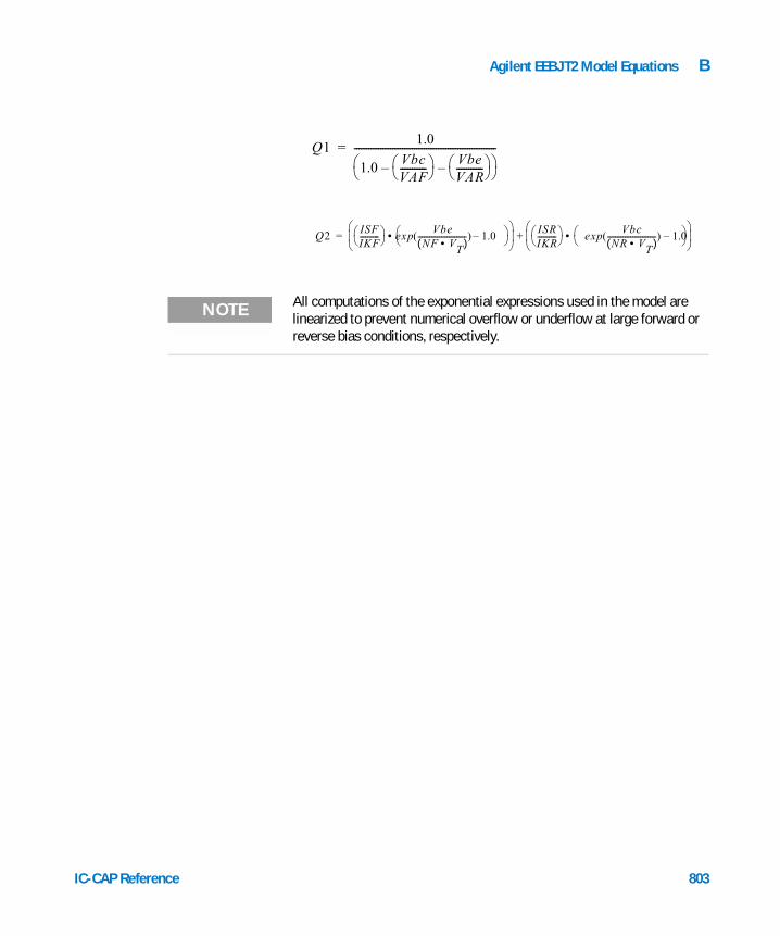
Agilent EEBJT2 Model Equations B
IC-CAP Reference
Q11.0
1.0VbcVAF----------- Vbe
VAR----------- ––
-----------------------------------------------------------=
Q2ISFIKF---------- exp
VbeNF VT•( )-------------------------( ) 1.0–
• ISR
IKR---------- exp
VbcNR VT•( )-------------------------( ) 1.0–
•
+=
NOTE All computations of the exponential expressions used in the model are linearized to prevent numerical overflow or underflow at large forward or reverse bias conditions, respectively.
803

B Agilent EEBJT2 Model Equations
Base-Emitter and Base-Collector Capacitances
804
Diffusion and depletion capacitances are modeled for both junctions of the transistor model in a manner very similar to the Gummel-Poon model.
For Vbc ≤ FC • VJC
where
and
For Vbc > FC • VJC
For Vbe ≤ FC • VJE
where
For Vbe > FC • VJE
Cbc Cbcdiffusion Cbcdepletion+=
Cbcdiffusion TR Icr•=
CbcdepletionCJC
1.0VbcVJC----------- –
MJC------------------------------------------------=
CbcdepletionCJC
1.0 FC–( )MJC--------------------------------------- 1.0
MJC Vbc FC VJC•( )–( )•VJC 1.0 FC–( )•
--------------------------------------------------------------------- +
•=
Cbe Cbediffusion Cbedepletion+=
CbedepletionCJE
1.0VbeVJE---------- –
MJE-----------------------------------------------=
IC-CAP Reference

Agilent EEBJT2 Model Equations B
IC-CAP Reference
The diffusion capacitance for Cbe is somewhat differently formulated vs. that of Cbc. The transit time is not a constant for the diffusion capacitance for Cbe, but is a function of both junction voltages, formulated in a manner similar to the modified Gummel-Poon model. The total base-emitter charge is equal to the sum of the base-emitter depletion charge (which is a function of Vbe only) and the so-called transit charge (which is a function of both Vbe and Vbc).
where
and
and
CbedepletionCJE
1.0 FC–( )MJE--------------------------------------- 1.0
MJE Vbe FC VJE•( )–( )•VJE 1.0 FC–( )•
-------------------------------------------------------------------- +
•=
Qtransit TffIcfQb------- •=
Tff TF 1.0 XTFIcf
Icf ITF+----------------------- 2.0
expVbc
1.44 VTF•---------------------------( )• • +
•=
Cbediffusion Vbe( )Vbe∂
∂Qtransit=
Cbediffusion Vbc( )Vbc∂
∂Qtransit=
805

806
B Agilent EEBJT2 Model Equations
Equivalent Circuit
Intrinsic Model(NPN or PNP)
+
-Vbe
+
-Vbc
IC-CAP Reference

Agilent EEBJT2 Model Equations B
IC-CAP Reference
Intrinsic Model
Cbc
Cbe
Ibc
Ibe
Ice
IcfIcr
Ib
Ic
Ie
+
-
Vbc
+
−
Vbe
807

B Agilent EEBJT2 Model Equations
References
808
1 J. J. Ebers and J. L. Moll. “Large Signal Behaviour of Junction Transistors,” Proc. I.R.E. 42, 1761 (1954).
2 H. K. Gummel and H. C. Poon. “An Integral Charge-Control Relation for Bipolar Transistors,” Bell Syst. Techn. J. 49, 115 (1970).
3 SPICE2: A Computer Program to Simulate Semiconductor Circuits, University of California, Berkeley.
4 P. C. Grossman and A. Oki. “A Large Signal DC Model for GaAs/GaxAl1-xAs Heterojunction Bipolar Transistors,” Proceedings of the 1989 IEEE Bipolar Circuits and Technology Meeting, pp. 258-262, September 1989.
IC-CAP Reference

Agilent 85190A IC-CAP 2008Reference
CAgilent EEFET3 Model Equations
Drain-Source Current 810
Dispersion Current (Idb) 816
Gate Charge Model 820
Output Charge and Delay 826
Gate Forward Conduction and Breakdown 827
Scaling Relations 828
References 831
This appendix describes the HPEEFET3 model equations used in IC-CAP.
809Agilent Technologies

C Agilent EEFET3 Model Equations
Drain-Source Current
810
The drain-source current model in Agilent EEFET3 is comprised of various analytic expressions that were developed through examination of gm vs. bias plots on a wide class of devices from various manufacturers. The expressions below are given for Vds > 0.0 V although the model is equally valid for Vds < 0.0 V. The model assumes the device is symmetrical, and one need only replace Vgs with Vgd and Vds with −Vds in order to obtain the reverse region (Vds < 0.0 V) equations. The gm, gds and Ids equations take on 4 different forms depending on the value of Vgs relative to some of the model parameters. The Ids expression is continuous through at least the second derivative everywhere.
if Vgs ≥ Vg and VDELT ≤ 0.0
else if VDELT > 0.0 and Vgs > Vgb
else if Vgs ≤ Vt
gmo GMMAX 1 GAMMA VDSO Vds–( )+{ }=
Idso GMMAX Vx Vgs( )VGO VTO+( )
2------------------------------------– VCH+
=
gdso GMMAX GAMMA Vgs VCH–( )•–=
gmo gmm Vgb( ) mgmmVgs Vgb–( )•+=
Idso gmm Vgb( ) Vgs Vgb–( )•mgmm
2---------------- Vgs Vgb–( )
2Idsm Vgb( )+ +=
gdso
∂ gmm Vgb( )( )
∂Vds------------------------------------ Vgs Vgb–( ) 1
2--- Vgs Vgb–( )2
∂mgmm∂Vds
--------------------•∂Vgb∂Vds-------------gmo–+=
IC-CAP Reference

Agilent EEFET3 Model Equations C
IC-CAP Reference
else
where
gmo 0.0=
Idso 0.0=
gdso 0.0=
gmo gmm Vgs( )=
Idso Idsm Vgs( )=
gdsoGMMAX
2-----------------------GAMMA Vgs VCH–( )–=
πVx Vgs( ) VGO VCH–( )–
VTO VGO–------------------------------------------------------------• 1+cos
•
gmm V( )GMMAX
2----------------------- 1 GAMMA VDSO Vds–( )+[ ]=
πVx V( ) VGO VCH–( )–
VTO VGO–------------------------------------------------------• 1+cos
•
Idsm V( )GMMAX
2----------------------- VTO VGO–( ) π⁄( ) π
Vx V( ) VGO VCH–( )–
VTO VGO–------------------------------------------------------•sin
=
Vx V( ) VTO VCH–( )–+ )
Vx V( ) V VCH–( ) 1 GAMMA VDSO Vds–( )+[ ]=
811

812
C Agilent EEFET3 Model Equations
VgVGO VCH–
1 GAMMA VDSO Vds–( )+--------------------------------------------------------------------- VCH+=
VtVTO VCH–
1 GAMMA VDSO Vds–( )+--------------------------------------------------------------------- VCH+=
VgbVGO VDELT–( ) VCH–
1 GAMMA VDSO Vds–( )+--------------------------------------------------------------------- VCH+=
mgmm
gmm∂
V∂---------------
V Vgb==
GMMAX π•2 VTO VGO–( )--------------------------------------- 1 GAMMA VDSO Vds–( )+[ ] 2
–=
π–VDELT
VTO VGO–-------------------------------•sin•
gmm Vgb( )GMMAX
2----------------------- 1 GAMMA VDSO Vds–( )+[ ]=
π–VDELT
VTO VGO–-------------------------------• 1+cos
•
Idsm Vgb( )GMMAX
2----------------------- VTO VGO–( ) π⁄( ) π–
VDELTVTO VGO–-------------------------------•sin
=
VGO VDELT VTO––( ) )+
∂ gmm Vgb( )( )
∂Vds----------------------------------- GMMAX
2-----------------------– GAMMA π– VDELT
VTO VGO–-------------------------------• 1+cos
=
IC-CAP Reference

Agilent EEFET3 Model Equations C
IC-CAP Reference
The preceding relations for Idso, gmo and gdso can now be substituted in the following equations that model the current saturation and output conductance. This portion of the model can be recognized from the work of Curtice [1].
These expressions do an excellent job of fitting GaAs FET I-V characteristics in regions of low power dissipation; they will also fit pulsed (isothermal) I-V characteristics. To model negative conductance effects due to self-heating, the thermal model of Canfield was incorporated [2]. With this final enhancement, the DC expressions for Ids and associated conductances become:
∂mgmm∂Vds
--------------------GMMAX π•VTO VGO–( )
----------------------------------- GAMMA( ) 1 GAMMA VDSO Vds–( )+[ ]=
π–VDELT
VTO VGO–-------------------------------•sin•
∂Vgb∂Vds-------------
VGO VDELT–( ) VCH–
1 GAMMA VDSO Vds–( )+[ ] 2----------------------------------------------------------------------------- GAMMA•=
g'm gmo 1 KAPA Vds•+( )3VdsVSAT-------------- tanh=
I'ds Idso 1 KAPA Vds•+( )3VdsVSAT-------------- tanh=
g'ds gdso 1 KAPA Vds•+( ) IdsoKAPA+{ }3VdsVSAT-------------- tanh=
Idso
3 1 KAPA Vds•+( )
VSAT-------------------------------------------------•
3VdsVSAT--------------
2sech+
813
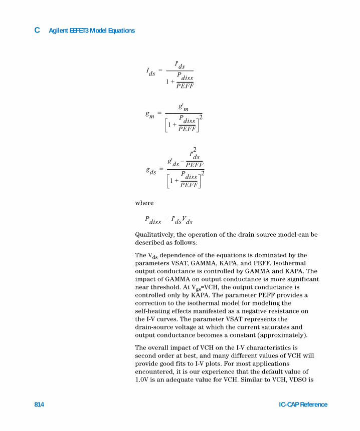
814
C Agilent EEFET3 Model Equations
where
Qualitatively, the operation of the drain-source model can be described as follows:
The Vds dependence of the equations is dominated by the parameters VSAT, GAMMA, KAPA, and PEFF. Isothermal output conductance is controlled by GAMMA and KAPA. The impact of GAMMA on output conductance is more significant near threshold. At Vgs=VCH, the output conductance is controlled only by KAPA. The parameter PEFF provides a correction to the isothermal model for modeling the self-heating effects manifested as a negative resistance on the I-V curves. The parameter VSAT represents the drain-source voltage at which the current saturates and output conductance becomes a constant (approximately).
The overall impact of VCH on the I-V characteristics is second order at best, and many different values of VCH will provide good fits to I-V plots. For most applications encountered, it is our experience that the default value of 1.0V is an adequate value for VCH. Similar to VCH, VDSO is
Ids
I'ds
1PdissPEFF---------------+
-------------------------=
gm
g'm
1PdissPEFF---------------+
2----------------------------------=
gds
g'ds
I'ds2
PEFF---------------–
1PdissPEFF---------------+
2----------------------------------=
Pdiss I'dsVds=
IC-CAP Reference

Agilent EEFET3 Model Equations C
IC-CAP Reference
a parameter that should be set rather than optimized. At Vds=VDSO, the drain-source model collapses to a single voltage dependency in Vgs. It is recommended that the user set VDSO to a typical Vds operating point in saturation. At this point, many of the parameters can be extracted right off a Ids-Vgs plot for Vds=VDSO or preferably, a gm(DC)-Vgs plot at Vds=VDSO.
When Vds=VDSO and PEFF is set large (to disable the self-heating model), the significance of the parameters VTO, VGO, VDELT, GMMAX are easily understood from a plot of gm(DC)-Vgs. GMMAX is the peak constant transconductance of the model that occurs at Vgs=VGO. The parameter VTO represents the gate-source voltage where gm goes to zero. If VDELT is set to a positive value, then it causes the transconductance to become linear at Vgs = VGO - VDELT with a slope equal to that of the underlying cosine function at this voltage. The parameter definitions are illustrated in the following figure.
Figure 21 Agilent EEFET3 gm-Vgs Parameters
gm(DC)
Vgs
GMMAX
VTO VGO
VGO-VDELT
815

C Agilent EEFET3 Model Equations
Dispersion Current (Idb)
816
Dispersion in a GaAs MESFET drain-source current is evidenced by the observation that the output conductance and transconductance beyond some transition frequency is higher than that inferred by the DC measurements. A physical explanation often attributed to this phenomenon is that the channel carriers are subject to being trapped in the channel-substrate and channel-surface interfaces. Under slowly varying signal conditions, the rate at which electrons are trapped in these sites is equal to the rate at which they are emitted back into the channel. Under rapidly varying signals, the traps cannot follow the applied signal and the high-frequency output conductance results.
The circuit used to model conductance dispersion consists of the elements RDB, CBS (these linear elements are also parameters) and the nonlinear source Idb(Vgs, Vds). The model is a large-signal generalization of the dispersion model proposed by Golio et al. [3]. At DC, the drain-source current is just the current Ids. At high frequency (well above the transition frequency), the drain source current will be equal to Ids(high frequency) = Ids(DC) + Idb. Linearization of the drain-source model yields the following expressions for y21 and y22 of the intrinsic Agilent EEFET3 model.
where
y21 gdsgs gdbgs
gdbgs1 jω CBS RDB••+--------------------------------------------------–+=
y22 gdsds gdbds1
RDB------------
gdbds1
RDB------------+
1 jω CBS RDB••+--------------------------------------------------–+ +=
gdsgs
Ids∂
Vgs∂------------=
IC-CAP Reference

Agilent EEFET3 Model Equations C
IC-CAP Reference
.
Evaluating these expressions at the frequencies ω=0 and ω=infinity produces the following results for transconductance and output conductance:
For ω=0,
For ω=infinity,
Between these 2 extremes, the conductances make a smooth transition, the abruptness of which is governed by the time constant τdisp = RDB • CBS. The frequency f0 at which the conductances are midway between these 2 extremes is defined as
gdsds
Ids∂
Vds∂------------=
gdbgs
Idb∂
Vgs∂------------=
gdbds
Idb∂
Vds∂------------=
Re y21[ ] gm gdsgs= =
Re y22[ ] gds gdsds= =
Re y21[ ] gm gdsgs gdbgs+= =
Re y22[ ] gds gdsds gdbds1
RDB------------+ += =
f01
2πτdisp--------------------=
817

818
C Agilent EEFET3 Model Equations
,
The parameter RDB should be set large enough so that its contribution to the output conductance is negligible. Unless you are specifically interested in simulating the device near f0, the default values of RDB and CBS will be adequate for most microwave applications.
The Agilent EEFET3 Ids model can be extracted to fit either DC or AC characteristics. In order to simultaneously fit both DC I-Vs and AC conductances, Agilent EEFET3 utilizes a simple scheme for modeling the Idb current source whereby different values of the same parameters can be used in the Ids equations. The DC and AC drain-source currents can be expressed as follows:
Parameters such as VGO that do not have an AC counterpart (i.e., there is no VGOAC parameter) have been found not to vary significantly between extractions utilizing DC measurements versus those utilizing AC measurements. The difference between the AC and DC values of Ids, plus an additional term that is a function of Vds only, gives the value of Idb for the dispersion model
where Idbp and its associated conductance are given by:
For Vds > VDSM and ,
IdsDC
Voltages Parameters,( ) Ids Voltages GMMAX VDELT VTO GAMMA,,,,(=
KAPA PEFF VTSO VGO VCH VDSO VSAT,,,,,, )
IdsAC
Voltages Parameters,( ) Ids Voltages GMMAXAC VDELTAC VTOAC,,,,(=
GAMMAAC KAPAAC PEFFAC VTSOAC VGO VCH VDSO VSAT, , , ),,,,
Idb Vgs Vds,( ) IdsAC
Vgs Vds,( ) IdsDC
Vgs Vds,( )– Idbp Vds( )+=
KDB 0≠
IC-CAP Reference

Agilent EEFET3 Model Equations C
IC-CAP Reference
For Vds < -VDSM and ,
For or ,
By setting the 7 high-frequency parameters equal to their DC counterparts, the dispersion model reduces to Idb = Idbp. Examination of the Idbp expression reveals that the additional setting of GDBM to zero disables the dispersion model entirely. Since the Idbp current is a function of Vds only, it will impact output conductance only. However, the current function will impact both gm and gds. For this reason, the model is primarily intended to utilized gm data as a means for tuning . Once this fitting is accomplished, the parameters GDBM, KDB and VDSM can be tuned to optimize the gds fit.
IdbpGDBMKDB
------------------ Vds VDSM–( ) KDB GDBM•( )1–
tan=
GDBM VDSM•+
gdbpGDBM
KDB GDBM Vds VDSM–( )2 1+• --------------------------------------------------------------------------------------------=
KDB 0≠
IdbpGDBMKDB
------------------ Vds VDSM+( ) KDB GDBM•( )1–
tan=
GDBM VDSM•–
gdbpGDBM
KDB GDBM Vds VDSM+( )2 1+• ---------------------------------------------------------------------------------------------=
VDSM– Vds VDSM≤ ≤ KDB 0=
Idsm GDBM Vds•=
gdbm GDBM=
IdsAC
IdsAC
819

C Agilent EEFET3 Model Equations
Gate Charge Model
820
The Agilent EEFET3 gate charge model was developed through careful examination of extracted device capacitances over bias. The model consists of simple closed form charge expressions whose derivatives fit observed bias dependencies in capacitance data. This capacitance data can be obtained directly from measured Y-parameter data.
The capacitance data is remarkably self-consistent. In other words, a single qg function’s derivatives will fit both C11 data and C12 data. The Agilent EEFET3 gate charge expression is:
where
This expression is valid for both positive and negative Vds. Symmetry is forced through the following smoothing functions proposed by Statz [4]:
C11
im y11[ ]
ω--------------------qg∂
Vgs∂------------= =
C12
im y12[ ]
ω--------------------
qg∂
Vds∂------------= =
qg Vj Vo,( )C11O C11TH–( )
2--------------------------------------------g Vj( ) C11TH Vj VINFL–( )+=
1 LAMBDA Vo VDSO–( )•+[ ]• C12SAT Vo•–
g Vj( ) Vj VINFL–DELTGS
3-----------------------
3DELTGS----------------------- Vj VINFL–( ) cosh
log+=
Vj12--- 2Vgs Vds– Vds
2DELTDS
2++
=
IC-CAP Reference

Agilent EEFET3 Model Equations C
IC-CAP Reference
Differentiating the gate charge expression wrt Vgs yields the following expression for the gate capacitance C11:
where
The gate transcapacitance C12 is defined as:
The Agilent EEFET3 topology requires that the gate charge be subdivided between the respective charge sources qgc and qgy. Although simulation could be performed directly from
Vo Vds2
DELTDS2
+=
C11 Vj Vo,( )C11O C11TH–( )
2-------------------------------------------- g' Vj( )• C11TH+=
1 LAMBDA Vo VDSO–( )•+[ ]•
g' Vj( )g Vj( )d
Vjd---------------- 1
3DELTGS----------------------- Vj VINFL–( )tanh+= =
C12 Vj Vo,( )qg∂
Vds∂------------
qg∂
Vj∂---------
Vj∂
Vds∂------------
qg∂
Vo∂---------
Vo∂
Vds∂------------+= =
C11 Vj Vo,( )12---•
Vds
Vds2
DELTDS2
+
----------------------------------------------- 1–=
C110 C11TH–2
--------------------------------------gVj C11THVj VINFL–+ LAMBDA C12SAT–•+
Vds
Vds2
DELTDS2
+
-----------------------------------------------•
821

822
C Agilent EEFET3 Model Equations
the nodal gate charge qg, division of the charge into branches permits the inclusion of the resistances RIS and RID that model charging delay between the depletion region and the channel. Agilent EEFET3 assumes the following form for the gate-drain charge in saturation:
which gives rise to a constant gate-drain capacitance in saturation. The gate-source charge qgc can now be obtained by subtracting the latter from the gate charge equation. Smoothing functions can then be applied to these expressions in saturation in order to extend the model’s applicable bias range to all Vds values.
These smoothing functions force symmetry on the qgy and qgc charges such that
at Vgc = Vgy. Under large negative Vds (saturation at the source end of the device), qgy and qgc swap roles, i.e:
The following continuous charge equations satisfy these constraints and are specified in terms of the gate charge:
where f1 and f2 are smoothing functions defined by
qgy Vgy( ) CGDSAT Vgy qgyo+•=
qgy qgc
qg2
------= =
qgc Vgc( ) CGDSAT Vgc qgco+•=
qgy Vgc Vgy,( ) qg Vgc Vgc Vgy–,( ) CGDSAT Vgc•–{ } f2•=
CGDSAT Vgy• f1•+
qgc Vgc Vgy,( ) qg Vgc Vgc Vgy–,( ) CGDSAT Vgy•–{ } f1•=
CGDSAT Vgc• f2•+
IC-CAP Reference

Agilent EEFET3 Model Equations C
IC-CAP Reference
and
The capacitances associated with these branch charge sources can be obtained through differentiation of the qgc and qgy equations and by application of the chain rule to the capacitances C11 and C12. The gate charge derivatives re-formulated in terms of Vgc and Vgy are:
The branch charge derivatives are:
f112--- 1
3DELTDS----------------------- Vgc Vgy–( ) tanh+=
f212--- 1
3DELTDS----------------------- Vgc Vgy–( ) tanh–=
Cggy
qg∂
Vgy∂------------ C12 Vgc Vgc Vgy–,( )–= =
Cggc
qg∂
Vgc∂------------ C11 Vgc Vgc Vgy–,( ) C12 Vgc Vgc Vgy–,( )+= =
Cgygy
qgy∂
Vgy∂------------ qg Vgc Vgc Vgy–,( ) CGDSAT Vgc•–{ }
f2∂
Vgy∂------------•= =
f2 Cggy CGDSAT Vgy
f1∂
Vgy∂------------ f1+••+•+
Cgygc
qgy∂
Vgc∂------------ qg Vgc Vgc Vgy–,( ) CGDSAT Vgc•–{ }
f2∂
Vgc∂------------•= =
f2 Cggc CGDSAT–[ ] CGDSAT Vgy
f1∂
Vgc∂------------••+•+
823

824
C Agilent EEFET3 Model Equations
where
Cgcgc
qgc∂
Vgc∂------------ qg Vgc Vgc Vgy–,( ) CGDSAT Vgy•–{ }
f1∂
Vgc∂------------•= =
f1 Cggc CGDSAT Vgc
f2∂
Vgc∂------------ f2+••+•+
Cgcgy
qgc∂
Vgy∂------------ qg Vgc Vgc Vgy–,( ) CGDSAT Vgy•–{ }
f1∂
Vgy∂------------•= =
f1 Cggy CGDSAT–[ ] CGDSAT Vgc
f2∂
Vgy∂------------••+•+
f1∂
Vgc∂------------
32 DELTDS•--------------------------------
3 Vgc Vgy–( )
DELTDS----------------------------------
2sech=
f1∂
Vgy∂------------f1∂
Vgc∂------------–=
f2∂
Vgc∂------------
f1∂
Vgc∂------------–=
f2∂
Vgy∂------------
f1∂
Vgc∂------------=
IC-CAP Reference

Agilent EEFET3 Model Equations C
IC-CAP Reference
When Vds=VDSO and VDSO>>DELTDS, the gate capacitance C11 reduces to a single voltage dependency in Vgs. Similar to the Ids model then, the majority of the important gate charge parameters can be estimated from a single trace of a plot. In this case, the plot of interest is C11-Vgs at Vds = VDSO.
The parameter definitions are illustrated in the following figure. The parameter DELTDS models the gate capacitance transition from the linear region of the device into saturation. LAMBDA models the slope of the C11-Vds characteristic in saturation. C12SAT is used to fit the gate transcapacitance (C12) in saturation.
Figure 22 Agilent EEFET3 C11-Vgs Parameters
C11
Vgs
C11O
VINFL
C11TH
DELTGS
825

C Agilent EEFET3 Model Equations
Output Charge and Delay
826
Agilent EEFET3 uses a constant output capacitance specified with the parameter CDSO. This gives rise to a drain-source charge term of the form
The drain-source current previously described in this section is delayed with the parameter TAU according to the following equation:
In the frequency domain, only the transconductance is impacted by this delay and the familiar expression for transconductance is obtained:
ym = gm • exp(−j • ω • TAU)
qds Vds( ) CDSO Vds•=
Ids t( ) Ids Vgs t TAU–( ) Vds t( ),( )=
IC-CAP Reference
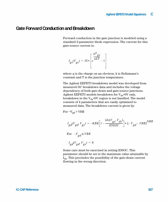
Agilent EEFET3 Model Equations C
Gate Forward Conduction and Breakdown
IC-CAP Reference
Forward conduction in the gate junction is modeled using a standard 2-parameter diode expression. The current for this gate-source current is:
where q is the charge on an electron, k is Boltzmann’s constant and T is the junction temperature.
The Agilent EEFET3 breakdown model was developed from measured DC breakdown data and includes the voltage dependency of both gate-drain and gate-source junctions. Agilent EEFET3 models breakdown for Vds>0V only, breakdown in the Vds<0V region is not handled. The model consists of 4 parameters that are easily optimized to measured data. The breakdown current is given by:
For −Vgd > VBR
For
Some care must be exercised in setting IDSOC. This parameter should be set to the maximum value attainable by Ids. This precludes the possibility of the gate-drain current flowing in the wrong direction.
Igs Vgs( ) IS e
qVgsnkT
------------1–•=
Igd Vgd Vgs,( ) KBK 1Ids Vgs Vds,( )
IDSOC----------------------------------– Vgd– VBR–( )NBR•–=
Vgd VBR≤–
Igd Vgd Vgs,( ) 0=
827

C Agilent EEFET3 Model Equations
Scaling Relations
828
Scaling of Agilent EEFET3 model parameters is accomplished through the use of the MDIF parameters UGW and NGF and the device parameters UGW (same name as the MDIF parameter) and N. From these 4 parameters, the following scaling relations can be defined:
where UGWnew represents the device parameter UGW, the new unit gate width.
Scaling will be disabled if any of the 4 scaling parameters are set to 0. The new Agilent EEFET3 parameters are computed internally by the simulator according to the following equations:
sfUGW
newN•
UGW NGF•----------------------------------=
sfgUGW N•
UGWnew
NGF•-------------------------------------------=
RISnew RIS
sf---------=
RIDnew RID
sf----------=
GMMAXnew
GMMAX sf•=
GMMAXACnew
GMMAXAC sf•=
PEFFnew
PEFF sf•=
PEFFACnew
PEFFAC sf•=
IC-CAP Reference

Agilent EEFET3 Model Equations C
IC-CAP Reference
RDBnew RDB
sf------------=
GDBMnew
GDBM sf•=
KDBnew KDB
sf------------=
ISnew
IS sf•=
KBKnew
KBK sf•=
IDSOCnew
IDSOC sf•=
RGnew RG
sfg--------=
RDnew RD
sf--------=
RSnew RS
sf-------=
CBSnew
CBS sf•=
C11Onew
C11O sf•=
C11THnew
C11TH sf•=
C12SATnew
C12SAT sf•=
CGDSATnew
CGDSAT sf•=
CDSOnew
CDSO sf•=
829

830
C Agilent EEFET3 Model Equations
Equivalent Circuit
Rdb
Ids
Igs
Igd
Qgc
Qgy
Rs
Rd
RgG’
G
S’
D’
D
SRis+ -
+ -Rid
C
Y
Cbs
B Idb Cdso
IC-CAP Reference

Agilent EEFET3 Model Equations C
References
IC-CAP Reference
1 W. R Curtice. “A MESFET model for use in the design of GaAs integrated circuits,” IEEE Transactions of Microwave Theory and Techniques, Vol. MTT-28, pp. 448-456, May 1980.
2 P. C. Canfield, “Modeling of frequency and temperature effects in GaAs MESFETs” IEEE Journal of Solid-State Circuits, Vol. 25, pp. 299-306,Feb. 1990.
3 J.M. Golio, M. Miller, G. Maracus, D. Johnson, “Frequency dependent electrical characteristics of GaAs MESFETs,” IEEE Trans. Elec. Devices, vol. ED-37, pp. 1217-1227, May 1990.
4 H. Statz, P. Newman, I. Smith, R. Pucel, H. Haus, “GaAs FET device and circuit simulation in SPICE,” IEEE Trans. Elec. Devices, vol. ED-34, pp. 160-169, Feb. 1987.
831

832
C Agilent EEFET3 Model Equations
IC-CAP Reference
Agilent 85190A IC-CAP 2008Reference
DAgilent EEHEMT1 Model Equations
Drain-Source Current 834
Dispersion Current (Idb) 842
Gate Charge Model 846
Output Charge and Delay 852
Gate Forward Conduction and Breakdown 853
Scaling Relations 854
References 857
This appendix describes the Agilent EEHEMT model equations used in IC-CAP.
833Agilent Technologies

D Agilent EEHEMT1 Model Equations
Drain-Source Current
834
The drain-source current model in Agilent EEHEMT1 is comprised of various analytic expressions that were developed through examination of gm vs. bias plots on a wide class of devices from various manufacturers. The expressions below are given for Vds > 0.0 V although the model is equally valid for Vds < 0.0 V. The model assumes the device is symmetrical, and one need only replace Vgs with Vgd and Vds with −Vds in order to obtain the reverse region (Vds < 0.0 V) equations. The gm, gds and Ids equations take on 4 different forms depending on the value of Vgs relative to some of the model parameters. The Ids expression is continuous through at least the second derivative everywhere.
if Vgs ≥ Vg
else if Vgs ≤ Vt
else
gmo GMMAX 1 GAMMA VDSO Vds–( )+{ }=
Idso GMMAX Vx Vgs( )VGO VTO+( )
2------------------------------------– VCH+
=
gdso GMMAX GAMMA Vgs VCH–( )•–=
gmo 0.0=
Idso 0.0=
gdso 0.0=
gmo gmm Vgs( )=
Idso Idsm Vgs( )=
IC-CAP Reference

Agilent EEHEMT1 Model Equations D
IC-CAP Reference
where
The following voltages define regions of operation that are used in the gm compression terms:
gdsoGMMAX
2-----------------------GAMMA Vgs VCH–( )–=
πVx Vgs( ) VGO VCH–( )–
VTO VGO–------------------------------------------------------------• 1+cos
•
gmm V( )GMMAX
2----------------------- 1 GAMMA VDSO Vds–( )+[ ]=
πVx V( ) VGO VCH–( )–
VTO VGO–------------------------------------------------------• 1+cos
•
Idsm V( )GMMAX
2----------------------- VTO VGO–( ) π⁄( ) π
Vx V( ) VGO VCH–( )–
VTO VGO–------------------------------------------------------•sin
=
Vx V( ) VTO VCH–( )–+ )
Vx V( ) V VCH–( ) 1 GAMMA VDSO Vds–( )+[ ]=
VgVGO VCH–
1 GAMMA VDSO Vds–( )+--------------------------------------------------------------------- VCH+=
VtVTO VCH–
1 GAMMA VDSO Vds–( )+--------------------------------------------------------------------- VCH+=
Vc VCO MU VDSO Vds–( )•+=
835

836
D Agilent EEHEMT1 Model Equations
For Vgs > Vc, the basic Idso, gmo and gdso relations are modified as follows:
for Vgs < Vb,
for Vgs ≥ Vb and b ≠ −1,
for Vgs ≥ Vb and b = −1
Vb VBC Vc+=
Va Vb VBA–=
gmocomp
gmo gmv Vgs Vds,( )–=
Idsocomp
Idso Idsv Vgs Vds,( )–=
gdsocomp
gdso gdsv Vgs Vds,( )–=
gmocomp
gmo a Vgs Va–( )b gmoff+–=
Idsocomp
Idsoa
b 1+------------ Vgs Va–( )b 1+
VBAb 1+
––=
gmoff Vgs Vb–( )•– Idsv Vb Vds,( )–
gdsocomp
gdso MU a Vgs Va–( )b gmoff+– gdsv Vb Vds,( )–=
gmocomp
gmo a Vgs Va–( )b gmoff+–=
Idsocomp
Idso a Vgs Va–( )log VBA( )log–[ ]–=
gmoff Vgs Vb–( )•– Idsv Vb Vds,( )–
IC-CAP Reference

Agilent EEHEMT1 Model Equations D
IC-CAP Reference
where
gdsocomp
gdsoMU a•
Vgs Va–( )---------------------------– MU gmoff•– gdsv Vb Vds,( )–=
agmv Vb Vds,( ) gmoff–
VBAb
-------------------------------------------------------=
bsvb VBA•
gmv Vb Vds,( ) gmoff–-------------------------------------------------------=
svb DELTGMVBC
ALPHA2
VBC2
+
-------------------------------------------------•=
gmv V Vds,( ) DELTGM ALPHA2
V Vc–( )2+ ALPHA–•=
Idsv V Vds,( ) DELTGM12--- V Vc–( ) ALPHA
2V Vc–( )2+
•=
ALPHA2
+V Vc–( ) ALPHA
2V Vc–( )2++
ALPHA-------------------------------------------------------------------------------------log•
ALPHA V Vc–( ) )•–
837

838
D Agilent EEHEMT1 Model Equations
In order to prevent gm from becoming negative at highgate-source biases, the following restriction is placed on the parameter DELTGM:
The preceding relations for , and can now be substituted in the following equations that model the current saturation and output conductance. This portion of the model can be recognized from the work of Curtice [1].
gdsv V Vds,( ) DELTGM MU12---
2 V Vc–( )2 ALPHA2
+
ALPHA2
V Vc–( )2+
----------------------------------------------------------
•=
ALPHA2
V Vc–( ) ALPHA2
V Vc–( )2++
-------------------------------------------------------------------------------------+
1V Vc–( )
ALPHA2
V Vc–( )2+
----------------------------------------------------------+•
ALPHA )–
gmoff gmo VCO VDSO,( )=
DELTGMgmoff
ALPHA2
VBC2
+ ALPHA–
---------------------------------------------------------------------------<
Idsocomp
gmocomp
gdsocomp
g'm gmocomp
1 KAPA Vds•+( )3VdsVSAT-------------- tanh=
I'ds Idsocomp
1 KAPA Vds•+( )3VdsVSAT-------------- tanh=
IC-CAP Reference
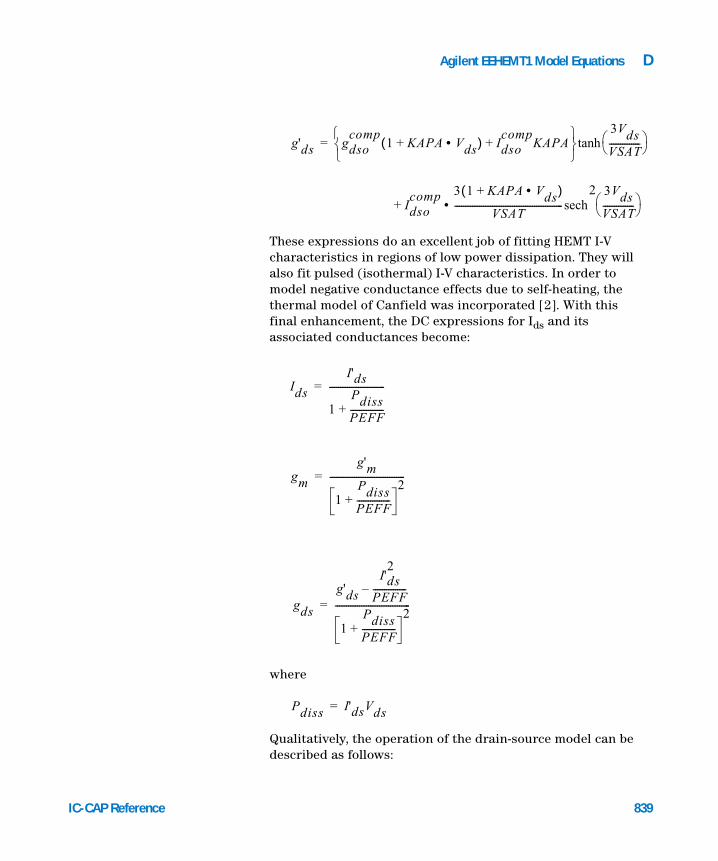
Agilent EEHEMT1 Model Equations D
IC-CAP Reference
These expressions do an excellent job of fitting HEMT I-V characteristics in regions of low power dissipation. They will also fit pulsed (isothermal) I-V characteristics. In order to model negative conductance effects due to self-heating, the thermal model of Canfield was incorporated [2]. With this final enhancement, the DC expressions for Ids and its associated conductances become:
where
Qualitatively, the operation of the drain-source model can be described as follows:
g'ds gdsocomp
1 KAPA Vds•+( ) Idsocomp
KAPA+ 3Vds
VSAT-------------- tanh=
Idsocomp 3 1 KAPA Vds•+( )
VSAT-------------------------------------------------•
3VdsVSAT--------------
2sech+
Ids
I'ds
1PdissPEFF---------------+
-------------------------=
gm
g'm
1PdissPEFF---------------+
2----------------------------------=
gds
g'ds
I'ds2
PEFF---------------–
1PdissPEFF---------------+
2----------------------------------=
Pdiss I'dsVds=
839
840
D Agilent EEHEMT1 Model Equations
The Vds dependence of the equations is dominated by the parameters VSAT, GAMMA, KAPA, and PEFF. Isothermal output conductance is controlled by GAMMA and KAPA. The impact of GAMMA on output conductance is more significant near threshold. At Vgs=VCH, the output conductance is controlled only by KAPA. The parameter PEFF provides a correction to the isothermal model for modeling the self-heating effects manifested as a negative resistance on the I-V curves. The parameter VSAT represents the drain-source voltage at which the current saturates and output conductance becomes a constant (approximately). The parameter MU also impacts the I-V curves in the gm compression region, but its effect is second order. In most cases, the gm fit is more sensitive to the parameter MU.
The overall impact of VCH on the I-V characteristics is second order at best, and many different values of VCH will provide good fits to I-V plots. For most applications encountered, it is our experience that the default value of 1.0V is an adequate value for VCH. Similar to VCH, VDSO is a parameter that should be set rather than optimized. At Vds = VDSO, the drain-source model collapses to a single voltage dependency in Vgs. It is recommended that the user set VDSO to a typical Vds operating point in saturation. At this point, many of the parameters
can be extracted right off a Ids-Vgs plot for Vds=VDSO or, preferably, a gm(DC)-Vgs plot at Vds=VDSO.
When Vds=VDSO and PEFF is set large (to disable the self-heating model), the significance of the parameters VTO, VGO, GMMAX, VCO, VBA, VBC, DELTGM and ALPHA are easily understood from a plot of gm(DC)-Vgs. GMMAX is the peak transconductance of the model that occurs at Vgs=VGO. The parameter VTO represents the gate-source voltage where gm goes to zero. Transconductance compression begins at Vgs=VCO. ALPHA controls the abruptness of this transition while DELTGM controls the slope of the gm characteristic in compression. At Vgs=VCO+VBC, the linear gm slope begins to tail-off and asymtotically approach zero. The shape of this “tail-off” region is controlled by the parameter VBA. The parameter definitions are illustrated in the following figure.
IC-CAP Reference
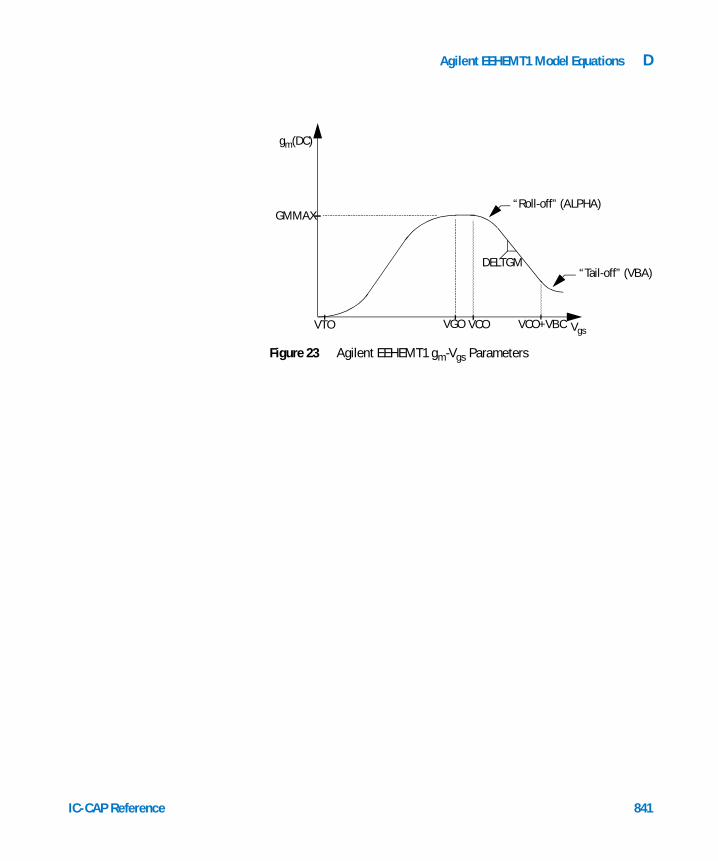
Agilent EEHEMT1 Model Equations D
IC-CAP Reference
Figure 23 Agilent EEHEMT1 gm-Vgs Parameters
gm(DC)
Vgs
GMMAX
VTO VGO VCO+VBCVCO
DELTGM
“Roll-off” (ALPHA)
“Tail-off” (VBA)
841

D Agilent EEHEMT1 Model Equations
Dispersion Current (Idb)
842
Dispersion in a GaAs MESFET or HEMT drain-source current is evidenced by the observation that the output conductance and transconductance beyond some transition frequency is higher than that inferred by the DC measurements. A physical explanation often attributed to this phenomenon is that the channel carriers are subject to being trapped in the channel-substrate and channel-surface interfaces. Under slowly varying signal conditions, the rate at which electrons are trapped in these sites is equal to the rate at which they are emitted back into the channel. Under rapidly varying signals, the traps cannot follow the applied signal and the high-frequency output conductance results.
The circuit used to model conductance dispersion consists of the elements RDB, CBS (these linear elements are also parameters) and the nonlinear source Idb(Vgs, Vds). The model is a large-signal generalization of the dispersion model proposed by Golio et al. [3]. At DC, the drain-source current is just the current Ids. At high frequency (well above the transition frequency), the drain source current will be equal to Ids(high frequency) = Ids(DC) + Idb. Linearization of the drain-source model yields the following expressions for y21 and y22 of the intrinsic Agilent EEHEMT1 model:
where
y21 gdsgs gdbgs
gdbgs1 jω CBS RDB••+--------------------------------------------------–+=
y22 gdsds gdbds1
RDB------------
gdbds1
RDB------------+
1 jω CBS RDB••+--------------------------------------------------–+ +=
gdsgs
Ids∂
Vgs∂------------=
IC-CAP Reference

Agilent EEHEMT1 Model Equations D
IC-CAP Reference
Evaluating these expressions at the frequencies ω = 0 and ω = infinity, produces the following results for transconductance and output conductance:
for ω = 0,
for ω = infinity,
Between these 2 extremes, the conductances make a smooth transition, the abruptness of which is governed by the time constant τdisp = RDB • CBS. The frequency f0 at which the conductances are midway between these 2 extremes is defined as
The parameter RDB should be set large enough so that its contribution to the output conductance is negligible. Unless the user is specifically interested in simulating the device near f0, the default values of RDB and CBS will be adequate for most microwave applications.
gdsds
Ids∂
Vds∂------------=
gdbgs
Idb∂
Vgs∂------------=
gdbds
Idb∂
Vds∂------------=
Re y21[ ] gm gdsgs= =
Re y22[ ] gds gdsds= =
Re y21[ ] gm gdsgs gdbgs+= =
Re y22[ ] gds gdsds gdbds1
RDB------------+ += =
f01
2πτdisp--------------------=
843

844
D Agilent EEHEMT1 Model Equations
The Agilent EEHEMT1 Ids model can be extracted to fit either DC or AC characteristics. In order to simultaneously fit both DC I-V characteristics and AC conductances, Agilent EEHEMT1 utilizes a simple scheme for modeling the Idb current source whereby different values of the same parameters can be used in the Ids equations. The DC and AC drain-source currents can be expressed as follows:
Parameters such as VGO that do not have an AC counterpart (i.e., there is no VGOAC parameter) have been found not to vary significantly between extractions utilizing DC measurements versus those utilizing AC measurements. The difference between the AC and DC values of Ids, plus an additional term that is a function of Vds only, gives the value of Idb for the dispersion model
where Idbp and its associated conductance are given by:
for Vds > VDSM and KDB ≠ 0,
IdsDC
Voltages Parameters,( ) Ids Voltages GMMAX VDELT VTO,,,,(=
GAMMA KAPA PEFF VTSO DELTGM,,,, ,
VGO VCH VDSO VSAT, , , )
IdsAC
Voltages Parameters,( ) IdsVoltages GMMAXAC VDELTAC,(,,(=
VTOAC, GAMMAAC KAPAAC' PEFFAC VTSOAC,,,,
DELTGMAC VGO VCH VDSO VSAT, , , , )
Idb Vgs Vds,( ) IdsAC
Vgs Vds,( ) IdsDC
Vgs Vds,( )– Idbp Vds( )+=
IdbpGDBMKDB
------------------ Vds VDSM–( ) KDB GDBM•( )1–
tan=
GDBM VDSM•+
IC-CAP Reference
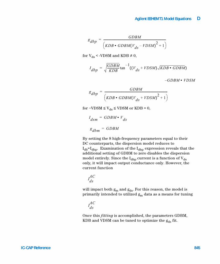
Agilent EEHEMT1 Model Equations D
IC-CAP Reference
for Vds < -VDSM and KDB ≠ 0,
for −VDSM ≤ Vds ≤ VDSM or KDB = 0,
By setting the 8 high-frequency parameters equal to their DC counterparts, the dispersion model reduces to Idb=Idbp. Examination of the Idbp expression reveals that the additional setting of GDBM to zero disables the dispersion model entirely. Since the Idbp current is a function of Vds only, it will impact output conductance only. However, the current function
will impact both gm and gds. For this reason, the model is primarily intended to utilized gm data as a means for tuning
Once this fitting is accomplished, the parameters GDBM, KDB and VDSM can be tuned to optimize the gds fit.
gdbpGDBM
KDB GDBM Vds VDSM–( )2 1+• --------------------------------------------------------------------------------------------=
IdbpGDBMKDB
------------------ Vds VDSM+( ) KDB GDBM•( )1–
tan=
GDBM VDSM•–
gdbpGDBM
KDB GDBM Vds VDSM+( )2 1+• ---------------------------------------------------------------------------------------------=
Idsm GDBM Vds•=
gdbm GDBM=
IdsAC
IdsAC
845

D Agilent EEHEMT1 Model Equations
Gate Charge Model
846
The Agilent EEHEMT1 gate charge model was developed through careful examination of extracted device capacitances over bias. The model consists of simple closed form charge expressions whose derivatives fit observed bias dependencies in capacitance data. This capacitance data can be obtained directly from measured Y-parameter data:
The capacitance data is remarkably self-consistent. In other words, a single qg function’s derivatives will fit both C11 data and C12 data. The Agilent EEHEMT1 gate charge expression is:
where
This expression is valid for both positive and negative Vds. Symmetry is forced through the following smoothing functions proposed by Statz [4]:
C11
im y11[ ]
ω--------------------qg∂
Vgs∂------------= =
C12
im y12[ ]
ω--------------------
qg∂
Vds∂------------= =
qg Vj Vo,( )C11O C11TH–
2---------------------------------------g Vj( ) C11TH Vj VINFL–( )+=
1 LAMBDA Vo VDSO–( )•+[ ]• C12SAT Vo•–
g Vj( ) Vj VINFL–DELTGS
3-----------------------
3DELTGS----------------------- Vj VINFL–( ) cosh
ln+=
Vj12--- 2Vgs Vds– Vds
2DELTDS
2++
=
IC-CAP Reference

Agilent EEHEMT1 Model Equations D
IC-CAP Reference
Differentiating the gate charge expression wrt Vgs yields the following expression for the gate capacitance C11:
where
The gate transcapacitance C12 is defined as:
The Agilent EEHEMT1 topology requires that the gate charge be subdivided between the respective charge sources qgc and qgy. Although simulation could be performed directly from
Vo Vds2
DELTDS2
+=
C11 Vj Vo,( )C11O C11TH–
2---------------------------------------g' Vj( ) C11TH+=
1 LAMBDA Vo VDSO–( )•+[ ]•
g' Vj( )g Vj( )d
Vjd---------------- 1
3DELTGS----------------------- Vj VINFL–( )tanh+= =
C12 Vj Vo,( )qg∂
Vds∂------------
qg∂
Vj∂---------
Vj∂
Vds∂------------
qg∂
Vo∂---------
Vo∂
Vds∂------------+= =
C11 Vj Vo,( )12---•
Vds
Vds2
DELTDS2
+
----------------------------------------------- 1–=
C110 C11TH–2
--------------------------------------g Vj( ) LAMBDA C12SAT–•+
Vds
Vds2
DELTDS2
+---------------------------------------------•
847

848
D Agilent EEHEMT1 Model Equations
the nodal gate charge qg, division of the charge into branches permits the inclusion of the resistances RIS and RID that model charging delay between the depletion region and the channel. Agilent EEHEMT1 assumes the following form for the gate-drain charge in saturation:
which gives rise to a constant gate-drain capacitance in saturation.
The gate-source charge qgc can now be obtained by subtracting the latter from the gate charge equation. Smoothing functions can then be applied to these
expressions in saturation in order to extend the model’s applicable bias range to all Vds values. These smoothing functions force symmetry on the qgy and qgc charges such that
at Vgc = Vgy. Under large negative Vds (saturation at the source end of the device), qgy and qgc swap roles, i.e:
The following continuous charge equations satisfy these constraints and are specified in terms of the gate charge:
where f1 and f2 are smoothing functions defined by
qgy Vgy( ) CGDSAT Vgy qgyo+•=
qgy qgc
qg2
------= =
qgc Vgc( ) CGDSAT Vgc qgco+•=
qgy Vgc Vgy,( ) qg Vgc Vgc Vgy–,( ) CGDSAT Vgc•–{ } f2•=
CGDSAT Vgy• f1•+
qgc Vgc Vgy,( ) qg Vgc Vgc Vgy–,( ) CGDSAT Vgy•–{ } f1•=
CGDSAT Vgc• f2•+
IC-CAP Reference

Agilent EEHEMT1 Model Equations D
IC-CAP Reference
and
The capacitances associated with these branch charge sources can be obtained through differentiation of the qgc and qgy equations and by application of the chain rule to the capacitances C11 and C12. The gate charge derivatives re-formulated in terms of Vgc and Vgy are:
The branch charge derivatives are:
f112--- 1
3DELTDS----------------------- Vgc Vgy–( ) tanh+=
f212--- 1
3DELTDS----------------------- Vgc Vgy–( ) tanh–=
Cggy
qg∂
Vgy∂------------ C12 Vgc Vgc Vgy–,( )–= =
Cggc
qg∂
Vgc∂------------ C11 Vgc Vgc Vgy–,( ) C12 Vgc Vgc Vgy–,( )+= =
Cgygy
qgy∂
Vgy∂------------ qg Vgc Vgc Vgy–,( ) CGDSAT Vgc•–{ }
f2∂
Vgy∂------------•= =
f2 Cggy CGDSAT Vgy
f1∂
Vgy∂------------ f1+••+•+
Cgygc
qgy∂
Vgc∂------------ qg Vgc Vgc Vgy–,( ) CGDSAT Vgc•–{ }
f2∂
Vgc∂------------•= =
f2 Cggc CGDSAT–[ ] CGDSAT Vgy
f1∂
Vgc∂------------••+•+
849

850
D Agilent EEHEMT1 Model Equations
where
When Vds=VDSO and VDSO>>DELTDS, the gate capacitance C11 reduces to a single voltage dependency in Vgs. Similar to the Ids model, the majority of the important gate charge parameters can then be estimated from a single trace of a
Cgcgc
qgc∂
Vgc∂------------ qg Vgc Vgc Vgy–,( ) CGDSAT Vgy•–{ }f1∂
Vgc∂------------•= =
f1 Cggc CGDSAT Vgc
f2∂
Vgc∂------------ f2+••+•+
Cgcgy
qgc∂
Vgy∂------------ qg Vgc Vgc Vgy–,( ) CGDSAT Vgy•–{ }
f1∂
Vgy∂------------•= =
f1 Cggy CGDSAT–[ ] CGDSAT Vgc
f2∂
Vgy∂------------••+•+
f1∂
Vgc∂------------3
2 DELTDS•--------------------------------3 Vgc Vgy–( )
DELTDS----------------------------------
2sech=
f1∂
Vgy∂------------
f1∂
Vgc∂------------–=
f2∂
Vgc∂------------f1∂
Vgc∂------------–=
f2∂
Vgy∂------------
f1∂
Vgc∂------------=
IC-CAP Reference

Agilent EEHEMT1 Model Equations D
IC-CAP Reference
plot. In this case, the plot of interest is C11-Vgs at Vds = VDSO. The parameter definitions are illustrated in the following figure.
The parameter DELTDS models the gate capacitance transition from the linear region of the device into saturation. LAMBDA models the slope of the C11-Vds characteristic in saturation. C12SAT is used to fit the gate transcapacitance (C12) in saturation.
Figure 24 Agilent EEHEMT1 C11-Vgs Parameters
C11
Vgs
C11O
VINFL
C11TH
DELTGS
851

D Agilent EEHEMT1 Model Equations
Output Charge and Delay
852
Agilent EEHEMT1 uses a constant output capacitance specified with the parameter CDSO. This gives rise to a drain-source charge term of the form
The drain-source current described previously, is delayed with the parameter TAU according to the following equation:
In the frequency domain, only the transconductance is impacted by this delay and the familiar expression for transconductance is obtained
ym = gm • exp(−j • ω • TAU)
qds Vds( ) CDSO Vds•=
Ids t( ) Ids Vgs t TAU–( ) Vds t( ),( )=
IC-CAP Reference

Agilent EEHEMT1 Model Equations D
Gate Forward Conduction and Breakdown
IC-CAP Reference
Forward conduction in the gate junction is modeled using a standard 2-parameter diode expression. The current for this gate-source current is:
where q is the charge on an electron, k is Boltzmann’s constant, and T is the junction temperature.
The Agilent EEHEMT1 breakdown model was developed from measured DC breakdown data and includes the voltage dependency of both gate-drain and gate-source junctions. Agilent EEHEMT1 models breakdown for Vds > 0V only, breakdown in the Vds < 0V region is not handled. The model consists of 4 parameters that are easily optimized to measured data. The breakdown current is given by:
for −Vgd > VBR
for −Vgd ≤ VBR
Some care must be exercised in setting IDSOC. This parameter should be set to the maximum value attainable by Ids. This precludes the possibility of the gate-drain current flowing in the wrong direction.
Igs Vgs( ) IS e
qVgsnkT
------------1–•=
Igd Vgd Vgs,( ) KBK 1Ids Vgs Vds,( )
IDSOC----------------------------------– Vgd– VBR–( )NBR•–=
Igd Vgd Vgs,( ) 0=
853

D Agilent EEHEMT1 Model Equations
Scaling Relations
854
Scaling of Agilent EEHEMT1 model parameters is accomplished through the use of the MDIF parameters UGW and NGF and the device parameters UGW (same name as the MDIF parameter) and N. From these 4 parameters, the following scaling relations can be defined:
where UGWnew represents the device parameter UGW, the new unit gate width.
Scaling will be disabled if any of the 4 scaling parameters are set to 0. The new Agilent EEHEMT1 parameters are computed internally by the simulator according to the following equations:
sfUGW
newN•
UGW NGF•----------------------------------=
sfgUGW N•
UGWnew
NGF•-------------------------------------------=
RISnew RIS
sf---------=
RIDnew RID
sf----------=
GMMAXnew
GMMAX sf•=
GMMAXACnew
GMMAXAC sf•=
DELTGMnew
DELTGM sf•=
DELTGMACnew
DELTGMAC sf•=
PEFFnew
PEFF sf•=
IC-CAP Reference

Agilent EEHEMT1 Model Equations D
IC-CAP Reference
PEFFACnew
PEFFAC sf•=
RDBnew RDB
sf------------=
GDBMnew
GDBM sf•=
KDBnew KDB
sf------------=
ISnew
IS sf•=
KBKnew
KBK sf•=
IDSOCnew
IDSOC sf•=
RGnew RG
sfg--------=
RDnew RD
sf--------=
RSnew RS
sf-------=
CBSnew
CBS sf•=
C11Onew
C11O sf•=
C11THnew
C11TH sf•=
C12SATnew
C12SAT sf•=
CGDSATnew
CGDSAT sf•=
855

856
D Agilent EEHEMT1 Model Equations
Equivalent Circuit
CDSOnew
CDSO sf•=
Rdb
Ids
Igs
Igd
Qgc
Qgy
Rs
Rd
RgG’
G
S’
D’
D
SRis+ -
+ -Rid
C
Y
Cbs
B Idb Cdso
IC-CAP Reference

Agilent EEHEMT1 Model Equations D
References
IC-CAP Reference
1 W. R. Curtice, “A MESFET model for use in the design of GaAs integrated circuits,” IEEE Transactions of Microwave Theory and Techniques, Vol. MTT-28, pp. 448-456, May 1980.
2 P. C. Canfield, “Modeling of frequency and temperature effects in GaAs MESFETs” IEEE Journal of Solid-State Circuits, Vol. 25, pp. 299-306, Feb. 1990.
3 J. M. Golio, M. Miller, G. Maracus, D. Johnson, “Frequency dependent electrical characteristics of GaAs MESFETs,” IEEE Trans. Elec. Devices, vol. ED-37, pp. 1217-1227, May 1990.
4 H. Statz, P. Newman, I. Smith, R. Pucel, H. Haus. “GaAs FET device and circuit simulation in SPICE,” IEEE Trans. Elec. Devices, vol. ED-34, pp. 160-169, Feb. 1987.
857

858
D Agilent EEHEMT1 Model Equations
IC-CAP Reference

Agilent 85190A IC-CAP 2008Reference
EControlling IC-CAP from Another Application
To Compile Using the Library 860
Details of Function Calls 862
Details of the LinkReturnS Structure 868
Other applications written in the C or C++ programming language can control IC-CAP via a library provided by IC-CAP. The library, libiclinklibs.a, consists of 6 function calls which enable the application to launch IC-CAP and communicate with it through an IPC (Inter-Process Communication) link.
The library allows the C application to send arbitrary PEL code to IC-CAP. The PEL code is then executed within IC-CAP. The context of the PEL code is 1 level above the macros in a Model. Therefore, the only variables available to the PEL code are the top-level System Variables. To see these variables, open the System Variables window using the menu Tools > System Variables in IC-CAP’s Main window.
The library libiclinklibs.a contains the following calls:int launch_iccap(const char *appName, const char *host, const char *iccapRoot, const char *altPath)int initialize_session()int terminate_session()int send_map(int *map, int length)int send_PEL(const char *PELText, int wait, char **errMsg, LinkReturnFuncT retfunc);int get_PEL_response(char **errMsg, LinkReturnFuncT
retfunc);
859Agilent Technologies

E Controlling IC-CAP from Another Application
To Compile Using the Library
860
Other files provided by IC-CAP to establish an IPC link include the following:
Platforms File Names
Solaris $ICCAP_ROOT/src/iclinklib.h
Solaris $ICCAP_ROOT/lib/sol2x/libiclinklibs.a$ICCAP_ROOT/lib/sol2x/libiclinklib.so
NOTE In IC-CAP 2004, the name of the static library changed from libiclinklib.a to libiclinklibs.a.
To compile your application with the static library, add -liclinklibs to the compile command along with -L$ICCAP_ROOT/lib/<pltfm> -liclinklibs where <pltfm> is sol2x or hpux10. In general, the static library (libiclinklibs.a) will be sufficient, but if you want to use the shared version (libiclinklib.sl or libiclinklib.so), it is also provided. To compile your application with the shared library, add -liclinklib to the compile command along with -L$ICCAP_ROOT/lib/<pltfm> -liclinklib where <pltfm> is sol2x or hpux10. For the Sun compiler, use the -Bstatic or -Bdynamic option to choose between the 2 libraries.
IC-CAP Reference

Controlling IC-CAP from Another Application E
Solaris Examples
IC-CAP Reference
To use the static iclinklibs library, and use shared libraries for all others (libc, etc.):cc program.c -L$ICCAP_ROOT/lib/sol2x -Bstatic -liclinklibs
-Bdynamic
To use static libraries for everything:cc program.c -L$ICCAP_ROOT/lib/sol2x -Bstatic -liclinklibs
To use shared libraries for everything:cc program.c -L$ICCAP_ROOT/lib/sol2x -Bdynamic -liclinklib
orcc program.c -L$ICCAP_ROOT/lib/sol2x -liclinklib
861

E Controlling IC-CAP from Another Application
Details of Function Calls
862
This section describes each function call available in the libiclinklibs.a library. The descriptions include available arguments, and the results returned, including error codes.
For an example of each function call, see the IC-CAP IPC Link example program ($ICCAP_ROOT/src/ipcexample.c). This example program takes control of IC-CAP. It then sends PEL commands to access variables and datasets in an npn model, performs a time-consuming task, and sends a pin mapping to IC-CAP and then accesses it.
launch_iccap
int launch_iccap(const char *appName, const char *host, const char *iccapRoot, const char *altPath)
launch_iccap invokes IC-CAP with the IPC link in place.
appName declares the name of the invoking program. This name cannot contain any spaces. This name will appear in the interactive dialog selector in IC-CAP as well as within a menu. If appName is NULL or the null string, the default link name will be Unnamed_Link.
host specifies the host’s name on which to run. If this string is not NULL, and if gethostent matches this host with gethostbyname(), then no remsh or rsh is used. If host is not NULL (or null string), and it returns a hostent with gethostbyname, then remsh or rsh will be used to invoke IC-CAP.
iccapRoot is the path to where IC-CAP has been installed on the machine on which it is to run. If iccapRoot is NULL, it is assumed that ICCAP_ROOT is or will be set in the environment and that $ICCAP_ROOT/bin is already in the path.
IC-CAP Reference

Controlling IC-CAP from Another Application E
IC-CAP Reference
altPath identifies a different path. Ordinarily, $ICCAP_ROOT/bin/iccap is used to invoke IC-CAP. Users often place a wrapper around this script to set up ICCAP_ROOT and LM_LICENSE_FILE. If this is the case, the alternate script can be named in this argument.
Returns
launch_iccap returns 0 if successful, or the following error codes:
-1 - Unable to determine current host.
-2 - Unable to fork.
initialize_session()
int initialize_session()
initialize_session attempts to gain control of the current IC-CAP session. Once initialized, PEL calls can be sent. IC-CAP is placed in a special mode on success of this call which will not raise any error dialogs. It also actively listens for calls from the link.
Returns
initialize_session() returns 0 if successful, or one of the following error codes:
-1 - IC-CAP is being used interactively. Message should be presented to user in this case telling them to set IC-CAP for Linked Mode.
-2 - General Communications Failure. IC-CAP is not responding as expected. The link has been broken.
-3 - The session is already running, and waiting for a PEL response from a prior send_PEL with wait==0. get_PEL_response must be called.
863

E Controlling IC-CAP from Another Application
terminate_session()
864
int terminate_session()
terminate_session relinquishes control of IC-CAP. This enables you to interactively use IC-CAP.
Returns
terminate_session() returns 0 if successful, or one of the following error codes:
-1 - Indicates that IC-CAP is in interactive mode.
-2 - Indicates a communications failure. When -2 is returned, the link is broken.
-3 - The session can’t be terminated. Waiting for a PEL response from a prior send_PEL with wait==0. get_PEL_response must be called.
send_PEL
int send_PEL(const char *PELText, int wait, char **errMsg, LinkReturnFuncT retfunc)
send_PEL sends PELText across the link to be executed within IC-CAP. initialize_session() must have been called successfully prior to this working. The text can be multiline or a single line of code. Each call to send_PEL essentially begins a new macro, so temporary variables within text will not persist between send_PEL calls. However, temporary variables can be used within multiline PELText. PELText should be null terminated.
wait specifies if send_PEL should wait for the PEL to finish before returning. If wait is nonzero, send_PEL will wait. If wait is 0, send_PEL will return immediately upon sending the PEL text to IC-CAP. The caller must then, at a later time, call get_PEL_response() to wait for the call to complete and collect the return status. See get_PEL_response.
If errMsg is not NULL and a PEL error occurs (noted by return of -3), it will be set to point to an error message returned from IC-CAP. The message will be a null
IC-CAP Reference

Controlling IC-CAP from Another Application E
IC-CAP Reference
terminated string and must be freed with free(). No memory is allocated if NULL is passed to send_PEL, or if no error occurs. errMsg is only meaningful when -3 is returned.
retfunc points to a function of type LinkReturnFuncT. This function will be invoked whenever IC-CAP calls one of the functions ICMSchar, ICMSint, ICMSreal, ICMSstr, or ICMSarray. The one argument to this function is a pointer to a LinkReturnS structure as shown in the following statement:typedef int (*LinkReturnFuncT)(struct LinkReturnS *);
For details about the structure, see “Details of the LinkReturnS Structure” on page 868.
Returns
send_PEL() returns 0 if successful, or one of the following error codes:
-1 - Indicates that IC-CAP is in interactive mode.
-2 - Indicates a communications failure. When -2 is returned, the link is broken.
-3 - PEL was executed, but an IC-CAP error occurred. Check errMsg for details.
-4 - PEL could not be sent, because there is a pending response caused by a prior send_PEL with wait==0.
get_PEL_response
int get_PEL_response(char **errMsg, LinkReturnFuncT retfunc)
get_PEL_response waits PEL from a prior send_PEL (with wait==0) to complete.
If errMsg is not NULL and a PEL error occurred (error code -3), it will be set to point to an error message returned from IC-CAP. The message will be a null terminated string and must be freed with free(). No memory will be allocated if NULL is passed to send_PEL, or if no error occurs. errMsg is only meaningful when -3 is returned.
865

866
E Controlling IC-CAP from Another Application
retfunc points to a function of type LinkReturnFuncT. This function is invoked when IC-CAP calls one of the functions ICMSchar, ICMSint, ICMSreal, ICMSstr, or ICMSarray. The one argument to this function is a pointer to a LinkReturnS structure as shown in the following statement:typedef int (*LinkReturnFuncT)(struct LinkReturnS *);
For details about the structure, see “Details of the LinkReturnS Structure” on page 868.
Returns
get_PEL_response() returns 0 if successful, or one of the following error codes:
-1 - Indicates that IC-CAP is in interactive mode.
-2 - Indicates a communications failure. When -2 is returned, the link is broken.
-3 - PEL was executed, but an IC-CAP error occurred. Check errMsg for details.
-4 - There were no prior send_PEL calls with wait==0 to wait for.
send_map
int send_map(int *pinMap, int numPins)
send_map sends a new pin matrix mapping to IC-CAP for use with ICMSpin() or SPECSpin(). The indices of the pinMap array correspond to the actual pins in the hardware. The values of pinMap correspond to the logical pad numbers associated with the pins. For example, if pinMap[5]=12, a call to SPECSpin(5) would return 12. If hardware contains no 0 pin, load pinMap[0] with -1.
Returns
send_map() returns 0 if successful, or one of the following error codes:
-1 - indicates that IC-CAP is in interactive mode.
-2 - indicates a communications failure. When -2 is returned, the link is broken.
IC-CAP Reference

Controlling IC-CAP from Another Application E
IC-CAP Reference
-3 - Map cannot be sent. Waiting for a PEL response from a prior send_PEL with wait==0. get_PEL_response must be called.
867

E Controlling IC-CAP from Another Application
Details of the LinkReturnS Structure
868
struct LinkReturnS {char type;int indx;int asize;union{char c_val;
int i_val;double r_val;double *a_val;char *s_val;
} value;};
type is a single character denoting type of data being passed: I (Int), C (Char), R (Real), S (String) or X (array).
indx refers to the index field of an ICMSXXXX function call. This is the index into which ICMS is to place the data.
asize is the size of the array that is passed in. This is 1 for type I, C, and R. For S, it is the length of the array. For X, it is the number of points in the data array.
union contains arguments where each x_val corresponds to the type character.
IC-CAP Reference

Agilent 85190A IC-CAP 2008Reference
FICCAP_FUNC Statement
The PEL statement ICCAP_FUNC replaced MENU_FUNC to reflect the fact that many objects you act on are not menu-related. (Note: Existing macros using the MENU_FUNC statement will still work but we recommend you create new macros using ICCAP_FUNC.)
The form of the PEL statement isICCAP_FUNC()
where () contains at least two arguments, each enclosed in quotation marks, separated by a comma
• The first argument is the name of the object on which you want to act
• The second argument is the action you want to perform
• Optional arguments can be used to anticipate prompts during execution, namely for filenames for reading or writing
An example is shown next: iccap_func("/CGaas1/dc/DeviceParameterSet","Memory Store")
where
CGaas1 is the model name
dc is the DUT name
DeviceParameterSet is the object on which to act
Memory Store is the action to perform on DeviceParameterSet (the object)
869Agilent Technologies

F ICCAP_FUNC Statement
The ThirdParameter
870
The optional arguments anticipate the need for information required to continue macro execution. If the argument is not included, and information is required, a dialog box appears prompting the user for the information. Usually, the optional arguments are file names used when reading from or writing to files. The following example shows how this optional argument is used to specify the file fileName.mdm from which to import data. This anticipates the need for a file name prompt and so avoids interrupting execution.
Example
iccap_func("CGaas1/dc/igvg_0vs","Import Data", "fileName.mdm")To successfully create macros with the ICCAP_FUNC statement, you must understand the hierarchy of the objects and specify the exact names of objects and actions. A tree-like structure, shown next, illustrates the relationship of the objects.
IC-CAP|— Variables|— GUI Items
|— GUI Item|— Simulation Debugger|— Hardware
|— HPIB Analyzer|— PlotOptions|— MODEL(*)
|— Variables|— GUI Items
|— GUI Item|— Circuit|— PlotOptimizer|— PlotOptions|— Parameter Set|— MACRO(*)|— DUT(*)
|—Variables|— GUI Items
|— GUI Item|—Test Circuit|—Device Parameter Set|—SETUP(*)
|—Variables
IC-CAP Reference
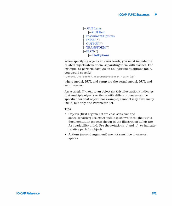
ICCAP_FUNC Statement F
IC-CAP Reference
|— GUI Items|— GUI Item
|—Instrument Options|—INPUT(*)|—OUTPUT(*)|—TRANSFORM(*)|—PLOT(*)
|— PlotOptions
When specifying objects at lower levels, you must include the related objects above them, separating them with slashes. For example, to perform Save As on an instrument options table, you would specify:“/model/DUT/setup/InstrumentOptions”,”Save As”
where model, DUT, and setup are the actual model, DUT, and setup names.
An asterisk (*) next to an object (in this illustration) indicates that multiple objects or items with different names can be specified for that object. For example, a model may have many DUTs, but only one Parameter Set.
Tips:
• Objects (first argument) are case-sensitive and space-sensitive; use exact spellings shown throughout this documentation (spaces shown in the illustration at left are for readability only). Use the notations ../ and ../.. to indicate relative path for objects.
• Actions (second argument) are not sensitive to case or spaces.
871

F ICCAP_FUNC Statement
Objects
IC-CAP
872
Specify using: "IC-CAP", "ic-cap" or "/"
Actions allowed
Change Directory (pg 905)Clear Status Errors (pg 907)Clear Status Output (pg 907)Close Error Log (pg 909)Close License Window (pg 910)Close Output Log (pg 910)Create Variable Table Variable (pg 912)Debug Off (pg 930)Diagnostics (pg 917)Exit/Exit! (pg 927)File Debug Off (pg 930)File Debug On (pg 929)License Status (pg 943)New Model (pg 950)Open Error Log (pg 952)Open Hardware (pg 952)Open Model (pg 953)Open Output Log (pg 953)Release License (pg 959)Save All (pg 964)Save All No Data (pg 964)Screen Debug Off (pg 930)Screen Debug On (pg 969)Set Variable Table Value (pg 981)Simulation Debugger (pg 983)Status Window (pg 984)Stop Simulator (pg 984)
IC-CAP Reference

ICCAP_FUNC Statement F
Variables
IC-CAP Reference
Specify using: “<path>/Variables” where <path> is the path to a Model, DUT, or Setup, or the slash (/) only to specify the top-level IC-CAP object.
Actions allowed
Open (pg 951)Print Via Server (pg 956)Save As (pg 964)Save As No Data (pg 965)Send To Printer (pg 973)Set Table Field Value (pg 978)Examples:
iccap_func("/Variables","Save As")iccap_func("/CGaas1/Variables","Save As")iccap_func("/CGaas1/dc/Variables","Save As")iccap_func("/myModel/myDut/mySetup/Variables","Save As")GUI Items
Specify using: “GUIItems”
Actions allowed Open (pg 951)Save As (pg 964)GUI Item
Specify using: “GUIItem”
Actions allowed
Add GUI (pg 900)Close GUI (pg 909)Close Single GUI (pg 910)Copy (pg 911)Destroy GUI (pg 916)Destroy Single GUI (pg 917)Display Modal GUI (pg 920)Display Modeless GUI (pg 920)Display Single Modal GUI (pg 921)Display Single Modeless GUI (pg 922)Set GUI Callbacks (pg 975)Set GUI Options (pg 976)873

F ICCAP_FUNC Statement
Simulation Debugger
874
Specify using: “SimulationDebugger”
Actions allowed
Close (pg 908)Manual Simulation (pg 947)Save Command File (pg 966)Save Input File (pg 966)Save Output File (pg 966)Simulation Debugger (pg 983)Example
iccap_func("ic-cap","Simulation Debugger")Hardware
Specify using: “Hardware”
Actions allowed
Add Active Instr (pg 899)Add Interface File (pg 900)Change Address (pg 904)Clear Active List (pg 906)Close Hardware (pg 910)Delete Active Instr (pg 914)Delete Interface File (pg 914)Diagnostics (pg 918)Disable Supplies (pg 919)Display Found Instrs (pg 920)Read from File (pg 956)Rebuild Active List (pg 958)Replace Interface File (pg 960)Run Self-Tests (pg 963)Write to File (pg 991)IC-CAP Reference

ICCAP_FUNC Statement F
HPIB Analyzer
IC-CAP Reference
Specify using: “Hardware/HPIBAnalyzer”
Actions allowed
Bus status (pg 903)Change Interface File (pg 905)Check Active Address (pg 906)I-O_Lock (pg 933)I-O_Reset (pg 934)I-O_Screen Debug ON (pg 934)I-O_Screen Debug OFF (pg 934)I-O_Unlock (pg 935)Listen Active Address (pg 944)Macro File Execute (pg 944)Macro File Specify (pg 946)Print Read Buffer (pg 955)Read String (pg 957)
Read String for Experts (pg 958)Search for Instruments (pg 969)Send Command Byte (pg 971)Send, Receive, and Print (pg 972)Send String (pg 973)Serial Poll (pg 974)Set Active Address (pg 974)Set Speed (pg 977)Set Timeout (pg 979)Talk Active Address (pg 985)Who Are You (pg 990)
875

F ICCAP_FUNC Statement
MODEL
876
Specify using: “/<name>” where <name> is the name of the model
Actions allowed
Clear Data/Both (pg 906)Clear Data/Measured (pg 906)Clear Data/Simulated (pg 906)Close All (pg 908)Copy (pg 911)Create Variable Table Variable (pg 912)Delete (pg 913)Display Plots (pg 921)Edit (pg 925)Export Dataset (pg 928)Import Data (pg 938)Import Measured Data (pg 939)Import Measured or Simulated Data (pg 940)Import Simulated Data (pg 940)Import Simulated or Measured Data (pg 941)Open (pg 951)Open DUT (pg 951)Open Macro (pg 953)New DUT (pg 949)New Macro (pg 950)Refresh Dataset (pg 959)Rename (pg 960)Save As (pg 964)Save As No Data (pg 965)Save Extracted Deck (pg 965)Set Variable Table Value (pg 981)Stop Simulator (pg 984)
Circuit
Specify using: "/<model>/Circuit" where <model> is the name of a model
Actions allowed
Copy (pg 911)Import Text (pg 942)Open (pg 951)Parse (pg 955)Save As (pg 964)Save As No Data (pg 965)IC-CAP Reference

ICCAP_FUNC Statement F
PlotOptimizer
IC-CAP Reference
Specify using: "/<model>/PlotOptimizer" where <model> is the name of a model
Actions allowed
Auto Set Min Max (pg 903)Auto Set Optimize or Auto Set And Optimize (pg 903)Clear Plot Optimizer (pg 907)Clear Table or Clear Parameter Table (pg 907)Disable All (pg 918)Enable All (pg 926)Optimize (pg 954)Recall Parameters (pg 958)Reset Min Max (pg 962)Reset Option Table (pg 962)Set Algorithm (pg 974)Set Error (pg 975)Set Table Field Value (pg 978)Simulate All (pg 983)Simulate Plot Inputs (pg 983)Store Parameters (pg 984)Tune Fast (pg 986)Tune Slow (pg 987)Undo Optim (pg 988)
PlotOptions
Plot Options are associated with the root IC-CAP object, models, and plots. To name the plot options, name the object with /PlotOptions appended (e.g., /PlotOptions, /modelname/PlotOptions, or /model/DUT/setup/plot/PlotOptions).Actions allowed
Set Table Field Value (pg 978)Example
iccap_func("myplot/PlotOptions","SetTableFieldValue","<access name>","<value>")iccap_func("/mymodel/PlotOptions","SetTableFieldValue","<access name>","<value>")
iccap_func("/mymodel/PlotOptions","SetTableFieldValue","<access name>","<value>")
where <access name> and <value> examples are listed in the following table:
NOTE To see the current <access name> and <value> settings, save the plot options from the Plot Options dialog then view in a text editor.
877

878
F ICCAP_FUNC Statement
Table 99 PlotOption Access Name and Value Examples
Description Access Names Values
Setting Trace Color on white
“On White[Data 0]” "2" (gxvt color index)
Setting Trace Color on black
“On Black[Data 3]” "4" (gxvt color index)
Setting Symbol “Symbol[Data 0]” “Circle”
Selecting Multicolor Curve setting
"Multicolor" "Display all curves with the configured trace color", "Change color with every curve", "Change color with each 2nd order curve", "Change color with each highest order curve"
Selecting Multicolor Curve color
"On White[Curve 0]" "2" (gxvt color index)
Selecting Data Representation
"Measured Trace","Simulated Trace","Transform Result"
"Symbols Only", "Solid Line", "Dashed Line". Solid Line with Symbols"
Layout and background settings
"Show Title", "Show Title", "Show Header",“Show Footer", "Show Legend","White Background","Show Area Tools"
"Yes", "No", "Automatic"
Selecting font and size
"Font Type", "Font Size"
"Arial for CAE", "12"
Selecting font and size of Annotation
"Annotation Font Name""Annotation Font Sz"
"Arial for CAE","9"
Enable/Disable Annotation
"Enable Annotation" "Yes", "No", "Automatic"
Annotation Location
"Annotation Location" "Upper Left", etc.
IC-CAP Reference

ICCAP_FUNC Statement F
IC-CAP Reference
Annotation text "Annotation Text" "W=10" or use an IC-CAP variable. Multiline text is available, each line must be separated by the string "\012"
Control Via PEL "PEL Control" "Yes", "No", "Automatic"
Specify annotation macro/transform
"PEL Transform" <name path>
Specify when updating the annotation
"PEL Call Type" "0" Only when plot is opened"1" Every time plot is refreshed
Table 99 PlotOption Access Name and Value Examples (continued)
Description Access Names Values
Parameter Set
Specify using: “/<model>/ParameterSet" where <model> is the name of a model
Actions allowed Copy (pg 911)Memory Recall (pg 948)Memory Store (pg 949)Open (pg 951)ReadOnlyValues (pg 957)Reset (pg 961)Save As (pg 964)Save As No Data (pg 965)MACRO
Specify using: "/<model>/<macroName>" where <model> is the name of a model, and <macroName> is the name of a macro within that model
Actions allowed
Copy (pg 911)Delete (pg 913)Execute (pg 927)Open (pg 951)879

880
F ICCAP_FUNC Statement
Rename (pg 960)Save As (pg 964)Save As No Data (pg 965)
IC-CAP Reference

ICCAP_FUNC Statement F
DUT
IC-CAP Reference
Specify using: "/<model>/<DUT>" where <model> is the name of a model, and <DUT> is the name of a DUT within that model.
Actions allowed
Clear Data/Both (pg 906)Clear Data/Measured (pg 906)Clear Data/Simulated (pg 906)Close All (pg 908)Close Branch (pg 908)Copy (pg 911)Create Variable Table Variable (pg 912)Delete (pg 913)Display Plots (pg 921)Export Dataset (pg 928)Extract (pg 929)Import Data (pg 938)Import Measured Data (pg 939)Import Measured or Simulated Data (pg 940)
Import Simulated Data (pg 940)Import Simulated or Measured Data (pg 941)Measure (pg 948)New Setup (pg 950)Open (pg 951)Open Branch (pg 951)Open Setup (pg 954)Optimize (pg 954)Rename (pg 960)Save As (pg 964)Save As No Data (pg 965)Set Variable Table Value (pg 981)Simulate (pg 983)
881

F ICCAP_FUNC Statement
Test Circuit
882
Specify using: "/<model>/<dut>/TestCircuit" where <model> is the name of a model and <dut> is the name of a DUT within that model.
Actions allowed
Copy (pg 911)Import Text (pg 942)Open (pg 951)Parse (pg 955)Save As (pg 964)Save As No Data (pg 965)Device Parameter Set
Specify using: "/<model>/<dut>/DeviceParameterSet" where <model> is the name of a model and <dut> is the name of a DUT within that model.
Actions allowed
Copy (pg 911)Memory Recall (pg 948)Memory Store (pg 949)Open (pg 951)ReadOnlyValues (pg 957)Reset (pg 961)Save As (pg 964)Save As No Data (pg 965)IC-CAP Reference

ICCAP_FUNC Statement F
SETUP
IC-CAP Reference
Specify using: "/<model>/<DUT>/<Setup>" where <model> is the name of a model, and <DUT> is the name of a DUT within that model, and <Setup> is a setup within that DUT.
Actions allowed
Calibrate (pg 904)Clear Data/Both (pg 906)Clear Data/Measured (pg 906)Clear Data/Simulated (pg 906)Close All (pg 908)Copy (pg 911)Create Variable Table Variable (pg 912)Delete (pg 913)Display Plots (pg 921)Export Data Measured (pg 928)Export Dataset (pg 928)Export Data Simulated (pg 929)Extract (pg 929)Import Create (pg 935)Import Create Header Only (pg 935)Import Create Measured (pg 936)Import Create Measured or Simulated (pg 936)Import Create Simulated (pg 937)Import Create Simulated or Measured (pg 937)
Import Data (pg 938)Import Delete (pg 939)Import Measured Data (pg 939)Import Measured or Simulated Data (pg 940)Import Simulated Data (pg 940)Import Simulated or Measured Data (pg 941)Measure (pg 948)New Input (pg 949)New Output (pg 949)New Plot (pg 949)New Transform (pg 949)Open (pg 951)Open Input (pg 952)Open Output (pg 952)Open Plot (pg 952)Open Transform (pg 952)Optimize (pg 954)Rename (pg 960)Save As (pg 964)Save As No Data (pg 965)Set Variable Table Value (pg 981)Simulate (pg 983)
883

F ICCAP_FUNC Statement
Instrument Options
884
Specify using: "/<model>/<DUT>/<Setup>/InstrumentOptions" where <model> is the name of a model, and <DUT> is the name of a DUT within that model, and <Setup> is a setup within that DUT.
Actions allowed
Open (pg 951)Save As (pg 964)Save As No Data (pg 965)INPUT
Specify using: "/<model>/<DUT>/<Setup>/<Input>" where <model> is the name of a model, and <DUT> is the name of a DUT within that model, <Setup> is a setup within that DUT, and <Input> is the name of an input within the setup.”
Actions allowed
Copy (pg 911)Delete (pg 913)Dump To Stdout (pg 924)Edit (pg 925)Open (pg 951)Print Via Server (pg 956)Redisplay (pg 959)Rename (pg 960)Save As (pg 964)Save As No Data (pg 965)Send To Printer (pg 973)Set Table Field Value (pg 978)View (pg 990)IC-CAP Reference

ICCAP_FUNC Statement F
OUTPUT
IC-CAP Reference
Specify using: "/<model>/<DUT>/<Setup>/<Output>" where <model> is the name of a model, and <DUT> is the name of a DUT within that model, <Setup> is a setup within that DUT, and <Output> is the name of an output within the setup.
Actions allowed
Copy (pg 911)Delete (pg 913)Dump To Stdout (pg 924)Edit (pg 925)Open (pg 951)Print Via Server (pg 956)Redisplay (pg 959)Rename (pg 960)Save As (pg 964)Save As No Data (pg 965)Send To Printer (pg 973)Set Table Field Value (pg 978)View (pg 990)TRANSFORM
Specify using: "/<model>/<DUT>/<Setup>/<Transform>" where <model> is the name of a model, and <DUT> is the name of a DUT within that model, <Setup> is a setup within that DUT, and <Transform> is the name of a transform within the setup.
Actions allowed
Auto Set Min Max (pg 903)Clear Table or Clear Parameter Table (pg 907)Copy (pg 911)Delete (pg 913)Dump To Stdout (pg 924)Execute (pg 927)Open (pg 951)Print Via Server (pg 956)Recall Parameters (pg 958)Redisplay (pg 959)Rename (pg 960)Reset Min Max (pg 962)Reset Option Table (pg 962)Save As (pg 964)885

886
F ICCAP_FUNC Statement
Save As No Data (pg 965)Send To Printer (pg 973)Set Algorithm (pg 974)Set Error (pg 975)Set Table Field Value (pg 978)Store Parameters (pg 984)Tune Fast (pg 986)Tune Slow (pg 987)Undo Optim (pg 988)View (pg 990)
PLOT
Specify using: “/<model>/<DUT>/<Setup>/<Plot>” where <model> is the name of a model, and <DUT> is the name of a DUT within that model, <Setup> is a setup within that DUT, and <Plot> is the name of a plot within the setup.
IC-CAP Reference

ICCAP_FUNC Statement F
Actions allowed
IC-CAP Reference
Add Global Region (pg 899)Add Trace Region (pg 901)Area Tools (pg 901)Area Tools Off (pg 901)Area Tools On (pg 902)Autoconfigure or Autoconfigure And Enable (pg 902)Autoscale (pg 902)Close (pg 908)Color (pg 911)Copy (pg 911)Copy to Clipboard (pg 912)Copy to Variables (pg 912)Data Markers (pg 913)Delete (pg 913)Delete Global Regions (pg 915)Delete Trace Regions (pg 915)Delete All User Regions (pg 916)Display Plot (pg 921)Hide Highlighted Curves (pg 932)Legend Off (pg 943)Legend On (pg 943)
Manual Rescale (pg 947)Mark Curve Highlighted (pg 947)Open (pg 951)Open Plot Optimizer (pg 954)Print Via Server (pg 956)Rescale (pg 961)Reset to Saved Options (pg 962)Redisplay (pg 959)Rename (pg 960)Replot (pg 960)Reset Global Region (pg 961)Reset Trace Region (pg 963)Save As (pg 964)Save As No Data (pg 965)Save Image (pg 966)Scale Plot (pg 967)Scale Plot Preview (pg 967)Scale RI Plot (pg 968)Show Highlighted Curves (pg 982)
Turn Off Marker (pg 987)Unmark All Highlighted Curves (pg 988)Unmark Highlighted Curve (pg 989)
887

888
F ICCAP_FUNC Statement
Delete User Region (pg 916)Disable All Traces (pg 918)Disable Plot (pg 919)Disable Trace (pg 919)Display Plot (pg 921)Display Plots (pg 921)Draw Diag Line (pg 922)Dump To Plotter (pg 923)Dump To Printer (pg 923)Dump Via Server (pg 924)Dump Via Server UI (pg 925)Edit (pg 925)Enable Plot (pg 926)Exchange Black-White (pg 927)Footer (pg 930)Footer Off (pg 931)Footer On (pg 931)Full Page Plot (pg 931)Header (pg 932)Header Off (pg 932)Header On (pg 932)Legend (pg 942)
Scale RI Plot Preview (pg 968)Select Error Region (pg 970)Select Plot (pg 970)Select Whole Plot (pg 971)Send To Printer (pg 973)Set Table Field Value (pg 978)Set Target Vs Simulated (pg 979)Set Trace As Both (pg 980)Set User Region (pg 980)Show Absolute Error (pg 981)Show Relative Error (pg 982)Text Annotation (pg 985)Text Annotation Off (pg 985)Text Annotation On (pg 986)Toggle Zoom (pg 986)Undo Zoom (pg 988)Unselect All (pg 989)Update Annotation (pg 990)View (pg 990)Zoom Plot (pg 991)
IC-CAP Reference

ICCAP_FUNC Statement F
Actions
IC-CAP Reference
Actions can be used to automate many IC-CAP dialog buttons and menu picks. The following tables cross-reference GUI buttons or menu picks to their corresponding actions.
Table 100 Hardware Setup Window Cross-Reference
Button/Menu Pick Action
Add Interface “Add Interface File” on page 900
Add to List “Add Active Instr” on page 899
Configure > Instrument Address “Change Address” on page 904
Delete “Delete Active Instr” on page 914
DeleteAll “Clear Active List” on page 906
Delete Interface “Delete Interface File” on page 914
File > Close Window “Close Hardware” on page 910
File > Open “Read from File” on page 956
File > Save “Write to File” on page 991
Instruments > Display “Display Found Instrs” on page 920
Instruments > Find “Search for Instruments” on page 969
Instruments > Self Test “Run Self-Tests” on page 963
Instruments > Usage “Diagnostics” on page 918
Instruments > Zero Sources “Disable Supplies” on page 919
Rebuild “Rebuild Active List” on page 958
Tools > Address > Check “Check Active Address” on page 906
Tools > Address > Listen “Listen Active Address” on page 944
Tools > Address > Set “Set Active Address” on page 974
Tools > Address > Talk “Talk Active Address” on page 985
Tools > Address > Who Are You? “Who Are You” on page 990
889

F ICCAP_FUNC Statement
Tools > Interface > Change “Change Interface File” on page 905
Tools > Interface > Lock “I-O_Lock” on page 933
Tools > Interface > Reset “I-O_Reset” on page 934
Tools > Interface > Status “Bus status” on page 903
Tools > Interface > Unlock “I-O_Unlock” on page 935
Tools > Macros > Execute “Macro File Execute” on page 944
Tools > Macros > Specify “Macro File Specify” on page 946
Tools > Send Receive > Display String “Print Read Buffer” on page 955
Tools > Send Receive > Read String for Experts “Read String for Experts” on page 958
Tools > Send Receive > Receive String “Read String” on page 957
Tools > Send Receive > Send Byte “Send Command Byte” on page 971
Tools > Send Receive > Send Receive Display “Send, Receive, and Print” on page 972
Tools > Send Receive > Send String “Send String” on page 973
Tools > Serial Poll “Serial Poll” on page 974
Tools > Settings > Timeout “Set Timeout” on page 979
View > Screen Debug “I-O_Screen Debug OFF” on page 934“I-O_Screen Debug ON” on page 934
Table 101 License Status Cross-Reference
Button/Menu Pick Action
OK “Close License Window” on page 910
Release “Release License” on page 959
Table 100 Hardware Setup Window Cross-Reference (continued)
Button/Menu Pick Action
890 IC-CAP Reference

ICCAP_FUNC Statement F
Table 102 Main Window Cross-Reference
Button/Menu Pick Action
File > Change Directory “Change Directory” on page 905
Edit > Copy “Copy” on page 911
Edit > Delete “Delete” on page 913
File > Edit “Edit” on page 925
File > Exit “Exit/Exit!” on page 927
File > New “New Model” on page 950
File > Open “Open Model” on page 953
File > Save As “Save All” on page 964“Save All No Data” on page 964
Tools > Hardware Setup “Open Hardware” on page 952
Tools > License Status “License Status” on page 943
Tools > Options > Diagnostics “Diagnostics” on page 917
Tools > Options > File Debug “File Debug On” on page 929“File/Screen Debug Off” on page 930
Tools > Options > Screen Debug “File/Screen Debug Off” on page 930“Screen Debug On” on page 969
Tools > Simulation Debugger “Simulation Debugger” on page 983
Tools > Stop Simulator “Stop Simulator” on page 984
Windows > Status Window “Status Window” on page 984
Table 103 Model Window Cross-Reference
Button/Menu Pick Action
Circuit folder, Import Text “Import Text” on page 942
Circuit folder, Parse “Parse” on page 955
Data > Plots > Display All “Display Plots” on page 921
IC-CAP Reference 891
F ICCAP_FUNC Statement
Duts/Setups folder, Add “New DUT” on page 949“New Setup” on page 950
DUTs/Setups, Extract/Optimize folder, Algorithm “Set Algorithm” on page 974
DUTs/Setups, Extract/Optimize folder, Error “Set Error” on page 975
DUTs/Setups, Extract/Optimize folder, Execute “Execute” on page 927
DUTs/Setups, Extract/Optimize folder, Recall Par “Recall Parameters” on page 958
DUTs/Setups, Extract/Optimize folder, Store Par “Store Parameters” on page 984
DUTs/Setups, Extract/Optimize folder, Tune Fast “Tune Fast” on page 986
DUTs/Setups, Extract/Optimize folder, Tune Slow “Tune Slow” on page 987
DUTs/Setups, Extract/Optimize folder, Undo Optim “Undo Optim” on page 988
DUTs/Setups, Extract/Optimize, Parameters folder, Autoset “Auto Set Min Max” on page 903
DUTs/Setups, Extract/Optimize, Parameters folder, Clear Table
“Clear Table or Clear Parameter Table” on page 907
DUTs/Setups, Extract/Optimize, Parameters folder, Reset “Reset Min Max” on page 962
DUTs/Setups, Instrument Options folder “Set Instrument Option Value” on page 977
DUTs/Setups, Measure/Simulate folder, Calibrate “Calibrate” on page 904
DUTs/Setups, Measure/Simulate folder, Clear > Measured, Simulated or Both Measured Simulated
“Clear Data/Simulated/Measured/Both” on page 906
DUTs/Setups, Measure/Simulate folder, Export Data “Export Data Measured” on page 928“Export Data Simulated” on page 929
DUTs/Setups, Measure/Simulate folder, Import Create “Import Create” on page 935“Import Create Header Only” on page 935“Import Create Measured” on page 936“Import Create Measured or Simulated” on page 936“Import Create Simulated” on page 937“Import Create Simulated or Measured” on page 937
DUTs/Setups, Measure/Simulate folder, Measure “Measure” on page 948
DUTs/Setups, Measure/Simulate folder, Simulate “Simulate” on page 983
DUTs/Setups, Measure/Simulate folder, View “View” on page 990
Table 103 Model Window Cross-Reference (continued)
Button/Menu Pick Action
892 IC-CAP Reference

ICCAP_FUNC Statement F
DUTs/Setups, Measure/Simulate and Plots folder “Set Table Field Value” on page 978
DUTs/Setups, Measure/Simulate folder, Input or Output, View, Dump to Stdout
“Dump To Stdout” on page 924
DUTs/Setups, Measure/Simulate folder, Input or Output, View, Print
“Dump To Plotter” on page 923“Dump To Printer” on page 923“Dump Via Server” on page 924“Send To Printer” on page 973
DUTs/Setups, Measure/Simulate, Setup Variables folder, System Variables
“Create Variable Table Variable” on page 912
DUTs/Setups, Setup Variables folder “Set Variable Table Value” on page 981
DUTs/Setups, Plots folder, Display Plot “Display Plot” on page 921
DUTs/Setups, Plots folder, Display Plots “Display Plots” on page 921
Edit > Cut Setup/Input “Import Delete” on page 939
Extract > Active Setup or Active DUT “Extract” on page 929
File > Close “Close All” on page 908
File > Export Data “Export Dataset” on page 928
File > Export Data > Extracted Deck “Save Extracted Deck” on page 965
File > Import Data “Import Data” on page 938“Import Measured Data” on page 939“Import Measured or Simulated Data” on page 940“Import Simulated Data” on page 940“Import Simulated or Measured Data” on page 941
File > Open “Open” on page 951“Open DUT” on page 951“Open Setup” on page 954“ReadOnlyValues” on page 957
File > Open (Input, Output, Transform, or Plot level selection) “Open Input/Output/Transform/Plot” on page 952
File > Open (for Macro) “Open Macro” on page 953
File > Print, (various dialogs) > Print “Print Via Server” on page 956
Table 103 Model Window Cross-Reference (continued)
Button/Menu Pick Action
IC-CAP Reference 893

F ICCAP_FUNC Statement
File > Save As “Save As” on page 964“Save As No Data” on page 965
Macro folder, New “New Macro” on page 950
Model Parameters folder, Memory Recall “Memory Recall” on page 948
Model Parameters folder, Memory Store “Memory Store” on page 949
Model Parameters folder, Reset “Reset” on page 961
Optimize > Active Setup or Active DUT “Optimize” on page 954
Tools > Plot Optimizer “Open Plot Optimizer” on page 954
Tools > Refresh Last Dataset “Refresh Dataset” on page 959
(various locations) > New “New Input/Output/Transform/Plot” on page 949
Table 104 Plot Optimizer Window Cross-Reference
Button/Menu Pick Action
Algorithm “Set Algorithm” on page 974
Parameters folder, Clear Table “Clear Table or Clear Parameter Table” on page 907
Error “Set Error” on page 975
Options folder, Print Settings “Dump To Plotter” on page 923“Dump To Printer” on page 923“Dump Via Server” on page 924“Send To Printer” on page 973
File > Clear Plot Optimizer “Clear Plot Optimizer” on page 907
File > Reset Option Table “Reset Option Table” on page 962
File > Close “Close” on page 908
Optimize > Tune Fast “Tune Fast” on page 986
Optimize > Tune Slow “Tune Slow” on page 987
Tools > Undo Optim “Undo Optim” on page 988
Table 103 Model Window Cross-Reference (continued)
Button/Menu Pick Action
894 IC-CAP Reference

ICCAP_FUNC Statement F
Plots > Disable All “Disable All” on page 918
Plots > Enable All “Enable All” on page 926
Simulate > plot name “Simulate Plot Inputs” on page 983
Simulate > Simulate All “Simulate All” on page 983
Tools > AutoSet Min and Max “Auto Set Min Max” on page 903
Tools > Recall Parameters “Recall Parameters” on page 958
Tools > Reset Min and Max “Reset Min Max” on page 962
Tools > Store Parameters “Store Parameters” on page 984
Table 105 Plots Window Cross-Reference
Button/Menu Pick Action
File > Close “Close” on page 908
File > Print “Dump Via Server UI” on page 925
File > Save Image “Save Image” on page 966
Optimizer > Autoconfigure and Enable “Autoconfigure or Autoconfigure And Enable” on page 902
Optimizer > Disable All Traces “Disable All Traces” on page 918
Optimizer > Enable/Disable Plot “Disable Plot” on page 919“Enable Plot” on page 926
Optimizer > Global Region > Delete All “Delete Global Regions” on page 915
Optimizer > Global Region > Reset “Reset Global Region” on page 961
Optimizer > Open Optimizer “Open Plot Optimizer” on page 954
Optimizer > trace > Disable “Disable Trace” on page 919
Optimizer > trace > Set as Both Target and Simulated “Set Trace As Both” on page 980
Optimizer > trace > Set as Target vs. “Set Target Vs Simulated” on page 979
Optimizer > trace > Trace Optimizer Region > Add “Add Trace Region” on page 901
Table 104 Plot Optimizer Window Cross-Reference (continued)
Button/Menu Pick Action
IC-CAP Reference 895

F ICCAP_FUNC Statement
Optimizer > trace > Trace Optimizer Region > DeleteAll “Delete Trace Regions” on page 915
Optimizer > trace > Trace Optimizer Region > Reset “Reset Trace Region” on page 963
Options > Autoscale “Autoscale” on page 902
Options > Copy to Clipboard “Copy to Clipboard” on page 912
Options > Copy to Variables “Copy to Variables” on page 912
Options > Draw Diag Line “Draw Diag Line” on page 922
Options > Edit Definition “Edit” on page 925
Options > Error > Select Error Region “Select Error Region” on page 970
Options > Error > Select Whole Plot “Select Whole Plot” on page 971
Options > Error > Show Absolute Error “Show Absolute Error” on page 981
Options > Error > Show Relative Error “Show Relative Error” on page 982
Options > Manual rescale “Manual Rescale” on page 947“Scale Plot/Scale Plot Preview” on page 967“Scale RI Plot/Scale RI Plot Preview” on page 968
Options > Replot “Replot” on page 960
Options > Rescale “Rescale” on page 961
Options > Session Settings > Area Tools “Area Tools” on page 901
Options > Session Settings > Color “Color” on page 911
Options > Session Settings > Exchange Black-White “Exchange Black-White” on page 927
Options > Session Settings > Footer “Footer” on page 930
Options > Session Settings > Header “Header” on page 932
Options > Session Settings > Legend “Legend” on page 942
Options > Session Settings > Reset to Saved Options “Reset to Saved Options” on page 962
Options > Session Settings > Text Annotation “Text Annotation” on page 985
Options > Update Annotation “Update Annotation” on page 990
Plots > Full Page Plot “Full Page Plot” on page 931
Table 105 Plots Window Cross-Reference (continued)
Button/Menu Pick Action
896 IC-CAP Reference
ICCAP_FUNC Statement F
Plots > Select Plot “Select Plot” on page 970
Plots > Undo Zoom “Undo Zoom” on page 988
Plots > Unselect All “Unselect All” on page 989
Plots > Zoom Plot “Zoom Plot” on page 991
Table 106 Simulation Debugger Window Cross-Reference
Button/Menu Pick Action
File > Close “Close” on page 908
File > Manual Simulation “Manual Simulation” on page 947
File > Save Command File File > Save Input File File > Save Output File
“Save Input/Command/Output File” on page 966
Table 107 Status Window Cross-Reference
Button/Menu Pick Action
File > Clear > Errors “Clear Status Errors” on page 907
File > Clear > Outputs “Clear Status Output” on page 907
File > Close Error Log “Close Error Log” on page 909
File > Close Output Log “Close Output Log” on page 910
File > Open Error Log “Open Error Log” on page 952
File > Open Output Log “Open Output Log” on page 953
Table 108 System GUI Items Cross-Reference
Button/Menu Pick Action
Add, Add Child “Add GUI” on page 900
Table 105 Plots Window Cross-Reference (continued)
Button/Menu Pick Action
IC-CAP Reference 897

F ICCAP_FUNC Statement
Close GUI “Close GUI” on page 909
Close Single GUI “Close Single GUI” on page 910
Destroy GUI “Destroy GUI” on page 916
Destroy Single GUI “Destroy Single GUI” on page 917
Display Modal GUI “Display Modal GUI” on page 920
Display Modeless GUI “Display Modeless GUI” on page 920
Display Single Modal GUI “Display Single Modal GUI” on page 921
Display Single Modeless GUI “Display Single Modeless GUI” on page 922
Set GUI Callbacks “Set GUI Callbacks” on page 975
Set GUI Options “Set GUI Options” on page 976
Table 108 System GUI Items Cross-Reference (continued)
Button/Menu Pick Action
898 IC-CAP Reference

ICCAP_FUNC Statement F
Add Active Instr
IC-CAP Reference
Automates the functionality of the “Add to List” button in the Hardware Setup window’s Instrument Library field.
Valid Objects
Hardware
menu_func style command: "Add Active Instr"
Adds the instrument selected in the Instrument Library to the Instrument List. To execute this function manually, the user selects an instrument from the Instrument Library, then presses the "Add to List" button. This functionality is emulated in PEL by appending the instrument to be added in the format:
"library name.select code.address"
followed by "ok" to the end of the command string.
Where
library name is the instrument model number exactly as it is listed in the Instrument Library.select code is the bus address (in decimal notation) of the GPIB card.address is the address (in decimal notation) of instrument, as set on the instrument itself.
Example
iccap_func("Hardware","Add Active Instr","HP8510.7.16","ok")Add Global Region
Automates the Optimizer > Global Region > Add menu pick in a plot window.
Valid Objects
Plotmenu_func style command: none
Adds a global trace region without deleting existing global trace regions.
Example
iccap_func("./dc/fgummel/ibicvsve", "AddGlobalRegion","0.6", "0.8", "-8", "-3")! Specify plot number for Multiploticcap_func("./dc/fgummel/my_multiplot", "AddGlobalRegion",
"0.6", "0.8", "-8", "-3", "1")
899

F ICCAP_FUNC Statement
See Also
900
Delete Global Regions (pg 915)
Add GUI
Automates the functionality of the “Add” and “Add Child” buttons in the System GUI Items window.
Valid Objects
GUI Itemmenu_func style command: none
Adds Items to a GUI Items page or another GUI Item. You must specify the Item’s name and type code. To see the codes for all Item types, select the Show Codes button on the Properties dialog of a GUI Item.
Example
iccap_func("./GUIItems","Add GUI","ANewTable","TL")iccap_func("./ANewTable","Add GUI","Button","PB")See Also
Close GUI (pg 909), Close Single GUI (pg 910), Destroy GUI (pg 916), Destroy Single GUI (pg 917), Display Modal GUI (pg 920), Display Modeless GUI (pg 920), Display Single Modal GUI (pg 921), Display Single Modeless GUI (pg 922), Set GUI Callbacks (pg 975), Set GUI Options (pg 976)Add Interface File
Automates the functionality of the “Add Interface” button in the Hardware Setup window’s GPIB Interface field.
Valid Objects
Hardwaremenu_func style command: "Add Active Interface"
Adds a GPIB Interface to the system. If this function were executed manually, a dialog box would appear asking the user for the name of the interface to be added. This functionality is emulated in PEL by appending the interface to be added followed by “ok” to the end of the command string.
Example
iccap_func("Hardware","Add Interface File","hpib","ok")IC-CAP Reference

ICCAP_FUNC Statement F
Add Trace Region
IC-CAP Reference
Automates the Optimizer > trace > Trace Optimizer Region > Add menu pick in a plot window.
Valid Objects
Plotmenu_func style command: none
Adds a trace optimizer region for the specified trace without deleting existing trace optimizer regions.
Example
iccap_func("./dc/fgummel/ibicvsve", "AddTraceRegion", "Y Data 0", "0.6", "0.8", "-8", "-3")iccap_func("./dc/fgummel/bvsic", "AddTraceRegion", "Y Data 0", "1e-8", "1e-4", "20", "60")
! Specify plot number for Multiploticcap_func("./dc/fgummel/my_multiplot", "AddTraceRegion",
"Y Data 0", "1e-8", "1e-4", "20", "60", "1")
See Also
Delete Trace Regions (pg 915)Area Tools
Automates the Options > Session Settings > Area Tools menu pick in a plot window.Valid Objects
Plotmenu_func style command: none
Toggles the Area Tools on and off for the specified plot window.
Example
iccap_func("./dc/fgummel/bvsic", "AreaTools")! Specify plot number for Multiploticcap_func("./dc/fgummel/my_multiplot", "AreaTools", "1")! Apply to all plots in a Multiploticcap_func("./dc/fgummel/my_multiplot", "AreaTools")See Also
Area Tools Off (pg 901), Area Tools On (pg 902)Area Tools Off
Hides the Area Tools for the specified plot window.
Valid Objects
Plotmenu_func style command: none
Example
iccap_func("./dc/fgummel/bvsic", "AreaToolsOff")901

902
F ICCAP_FUNC Statement
! Specify plot number for Multiploticcap_func("./dc/fgummel/my_multiplot", "AreaToolsOff", "1")! Apply to all plots in a Multiploticcap_func("./dc/fgummel/my_multiplot", "AreaToolsOff")
See Also
Area Tools (pg 901), Area Tools On (pg 902)Area Tools On
Displays the Area Tools for the specified plot window.
Valid Objects
Plotmenu_func style command: none
Example
iccap_func("./dc/fgummel/bvsic", "AreaToolsOn")! Specify plot number for Multiploticcap_func("./dc/fgummel/my_multiplot", "AreaToolsOn", "1")! Apply to all plots in a Multiploticcap_func("./dc/fgummel/my_multiplot", "AreaToolsOn")See Also
Area Tools (pg 901), Area Tools Off (pg 901)Autoconfigure or Autoconfigure And Enable
Automates the Optimizer > Autoconfigure and Enable menu pick in a plot window
Valid Objects
Plotmenu_func style command: none
Automatically enables and configures the inputs in a Plot window.
Example
iccap_func("dc/fgummel/icibvsve", "Autoconfigure")iccap_func("dc/fgummel/icibvsve", "AutoconfigureAndEnable")! Specify plot number for Multiploticcap_func("dc/fgummel/my_multiplot", "Autoconfigure", "1")! Apply to all plots in a Multiploticcap_func("dc/fgummel/my_multiplot", "Autoconfigure")Autoscale
Automates the Options > Autoscale menu pick in a plot window
Valid Objects
Plotmenu_func style command: “Replot Data”
IC-CAP Reference

ICCAP_FUNC Statement F
IC-CAP Reference
Toggles whether the plot automatically rescales when the data changes.
Example
iccap_func("/CGaas1/dc/igvg_0vs/vs/ig_vs_vg", "Autoscale")! Specify plot number for Multiploticcap_func("/CGaas1/dc/igvg/my_multiplot", "Autoscale", "1")! Apply to all plots in a Multiploticcap_func("/CGaas1/dc/igvg/my_multiplot", "Autoscale")Auto Set Min Max
Automates the Tools > AutoSet Min Max menu pick in the Plot Optimizer window and the Auto Set button in the Extract/Optimize folder.
Valid Objects
Transform, Plot Optimizermenu_func style command: none
Sets minimum and maximum optimizer parameter values based on the value of the coefficient defined with the AUTOSET_COEFF variable. The default coefficient value is 5.
Example iccap_func(“./CGaas1/dc/igvg_0vs”,”Auto Set Min Max”)iccap_func(“./PlotOptimizer”,”Auto Set Min Max”)Auto Set Optimize or Auto Set And Optimize
Automates the Optimizer > Autoset Min/Max and Optimize menu pick in the Plot Optimizer window.
Valid Objects
Plot Optimizermenu_func style command: none
Sets minimum and maximum optimizer parameter values based on the value of the coefficient defined with the AUTOSET_COEFF variable then runs an optimization. The default coefficient value is 5.
Example
iccap_func(“./PlotOptimizer”,”AutoSetAndOptimize”)Bus status
Automates the functionality of the “Tools/Interface/Status” menu pick in the Hardware Setup window.
903

F ICCAP_FUNC Statement
Valid Objects
904
Hardware/HPIBAnalyzer
menu_func style command: "Bus status"
Provides information on the status of the current interface including:
• Name
• Select Code
• Bus Address
• System Controller State
• Active Controller State
• Talker State
• Listener State
• SRQ State
• NDAC State
This information is displayed in the IC-CAP/Status window and, if visible, the Hardware Setup window.
Example
iccap_func("Hardware/HPIBAnalyzer","Bus status")Calibrate
Automates the Measure/Simulate folder’s Calibrate button.
Valid Objects
Setupmenu_func style command: “Calibrate”
Performs calibration on the specified setup
Example
iccap_func("CGaas1/dc/igvg_0vs","Calibrate")Change Address
Automates the functionality of the Instrument Address spin box in the dialog box displayed by the Configure button in the Instrument List in the Hardware Setup window.
Valid Objects
Hardwaremenu_func style command: "Change Address"
IC-CAP Reference

ICCAP_FUNC Statement F
IC-CAP Reference
Sets the address of the specified instrument. If this function were executed manually, the desired new address would be read from the spin box in the Configuration Dialog Box when the OK button was pushed. This functionality is emulated in PEL by appending the old GPIB name string in the format:"library name.select code.address"
followed by "ok" and the new desired address followed by "ok" to the end of the command string.
Example
iccap_func("Hardware","Change Address","HP3577.7.18","ok","19","ok")Change Directory
Automates IC-CAP/Main File > Change Directory
Valid Objects
IC-CAP
menu_func style command: “Utilities/Change Directory”
Prompts for the name of a new directory to use as the current working directory. The directory prompt can be anticipated by the third argument.
Example
iccap_func("ic-cap","Change Directory","/users/me/my_other_work_dir")Change Interface File
Automates the functionality of the Tools > Interface > Change menu pick in the Hardware Setup window.
Valid Objects
Hardware/HPIBAnalyzermenu_func style command: "Change Interface File"
Changes the currently active GPIB interface. All further commands of the GPIB Analyzer will be directed to this new interface. If this function were executed manually, a dialog box would appear asking the user for the name of the new interface. This functionality is emulated in PEL by appending the name of the new interface followed by "ok" to the end of the command string.
Example
iccap_func("Hardware/HPIBAnalyzer","Change Interface File","new_name","ok")905
F ICCAP_FUNC Statement
Check Active Address
906
Automates the functionality of the Tools > Address > Check menu pick in the Hardware Setup window.
Valid Objects
Hardware/HPIBAnalyzermenu_func style command: "Check Active Address"
This function sends a serial poll to the device at the currently active address as previously set by a call to “Set Active Address.” The result is displayed in the IC-CAP/Status window and, if visible, the Hardware Setup window.
Example
iccap_func("Hardware/HPIBAnalyzer","Set Active Address","8","ok")iccap_func("Hardware/HPIBAnalyzer","Check Active Address")
Clear Active List
Automates the functionality of the DeleteAll button in the Hardware Setup window’s Instrument List field.
Valid Objects
Hardwaremenu_func style command: "Clear Active List"
Removes all instruments in all setups from the Active Instrument List.
Example
iccap_func("Hardware","Clear Active List")Clear Data/Simulated/Measured/Both
• Clear Data/Simulated
• Clear Data/Measured
• Clear Data/Both
Automates the Model Window's Data > Clear Active Setup Data functionality or the Clear button in the Measure/Simulate folder.
Valid Objects
Model, DUT, Setupmenu_func style commands were the same.
IC-CAP Reference

ICCAP_FUNC Statement F
IC-CAP Reference
Clears the specified type of data from the outputs and transforms of the named Model, named DUT, or named setup.
Examples
iccap_func("/CGaas1/dc/igvg_0vs","Clear Data/Simulated")iccap_func("/CGaas1/dc","Clear Data/Measured")iccap_func("/CGaas1","Clear Data/Both")Clear Plot Optimizer
Automates the File > Clear Plot Optimizer menu pick in the Plot Optimizer window.
Valid Objects
Plot Optimizermenu_func style command: none
Disables all traces and regions in the plots, disables all open plots, and clears the Parameters table.
Example
iccap_func(“./PlotOptimizer”,”Clear Plot Optimizer”)See Also
Clear Table or Clear Parameter Table (pg 907) Clear Status ErrorsClears Status window’s Warnings/Errors.
Valid Objects
IC-CAPmenu_func style command: none
Example
iccap_func("/","Clear Status Errors")Clear Status Output
Clears Status window’s IC-CAP Output.
Valid Objects
IC-CAPmenu_func style command: none
Example
iccap_func("/","Clear Status Output")Clear Table or Clear Parameter Table
Automates the Clear Table button on the Parameter folder in the Plot Optimizer window and in the Extract/Optimize folder.
907

F ICCAP_FUNC Statement
Valid Objects
908
Transform, Plot Optimizer
menu_func style command: none
Deletes all parameters and variables in the optimizer’s parameter folder.
Example
iccap_func(“./CGaas1/dc/igvg_0vs”,”Clear Table”)iccap_func(“./PlotOptimizer”,”Clear Table”)See Also
Clear Plot Optimizer (pg 907)Close
Automates the IC-CAP/Simulation Debugger or Plot window’s File > Close functionality.
Valid Objects
Simulation Debugger, Plotmenu_func style command: “Close”
Closes the Simulation Debugger or Plot window if open.
Example
iccap_func("Simulation Debugger","Close")! closed Simulation Debuggericcap_func("/npn/dc/fgummel/ibicvsve","Close")!closes plotClose All
Automates the Model window’s File > Close functionality.
Valid Objects
Model, DUT, Setupmenu_func style command: “Close All”
Closes the model window and all associated windows, or all plot windows within a named DUT or setup.
Example
iccap_func("/CGaas1","Close All")! closes model and all childreniccap_func("/CGaas1/dc","Close All")! closes all plots within DUTClose Branch
Automates the action of closing a DUT on the DUTs/Setups tree.
Valid Objects
DUTIC-CAP Reference

ICCAP_FUNC Statement F
IC-CAP Reference
menu_func style command: none
Closes a DUT on the DUTs/Setups tree. By default, if you fabricate new DUTs with iccap_func Add DUT, the branch will be in the open state. Use this iccap_func to close it.
Example
iccap_func(“/mymodel/mydut”,“Close Branch”)See Also
Open Branch (pg 951)Close Error Log
Automates the IC-CAP/Status window’s Close Error Log functionality.
Valid Objects
IC-CAPmenu_func style command: none
Closes the error log file.
Example
iccap_func("ic-cap","Close Error Log") Close GUIAutomates closing an instance of a GUI item.
Valid Objects
GUI Itemmenu_func style command: none
Closes the named instance of a GUI item. Although no longer displayed, the GUI item still reacts to modifications to the variables page, etc.
Example
iccap_func("/mdl/dut/orSet/GUIName","Close GUI","InstanceName")See Also
Add GUI (pg 900), Close Single GUI (pg 910), Destroy GUI (pg 916), Destroy Single GUI (pg 917), Display Modal GUI (pg 920), Display Modeless GUI (pg 920), Display Single Modal GUI (pg 921), Display Single Modeless GUI (pg 922), Set GUI Callbacks (pg 975), Set GUI Options (pg 976)909

F ICCAP_FUNC Statement
Close Hardware
910
Automates the functionality of the File > Close Window menu pick in the Hardware Setup window.
Valid Objects
Hardwaremenu_func style command: none
This function closes the Hardware Setup window.
Example
iccap_func("Hardware","Close Hardware")Close License Window
Automates the functionality of the OK button in the License Status window. The window must be currently displayed (either by a License Status call or by choosing Tools > License Status in the Main window).
Valid Objects
IC-CAPmenu_func style command: none
This function closes the License Status window.
Example
iccap_func("IC-CAP","Close License Window")Close Output Log
Automates the IC-CAP/Status window’s Close Output Log functionality.
Valid Objects
IC-CAPmenu_func style command: none
Closes the output log file.
Example
iccap_func("ic-cap","Close Output Log")Close Single GUI
Automates closing a single displayed GUI item.
Valid Objects
GUI ItemIC-CAP Reference

ICCAP_FUNC Statement F
IC-CAP Reference
menu_func style command: none
Closes the displayed GUI item. Although no longer displayed, the GUI item still reacts to modifications to the variables page, etc.
Example
iccap_func("/mdl/dut/orSet/GUIName","Close Single GUI")See Also
Add GUI (pg 900), Close GUI (pg 909), Destroy GUI (pg 916), Destroy Single GUI (pg 917), Display Modal GUI (pg 920), Display Modeless GUI (pg 920), Display Single Modal GUI (pg 921), Display Single Modeless GUI (pg 922), Set GUI Callbacks (pg 975), Set GUI Options (pg 976)Color
Automates the Options > Session Settings > Color menu pick in a plot window.
Valid Objects
Plot
Toggles between color and black and white. Each time you c all you either go to color or to black and white.
Example
iccap_func("/CGaas1/dc/igvg_0vs/vs/ig_vs_vg","Color")Copy
Automates copying an item to a new name, but does not permit undo or paste after completion.
Valid Objects
Model, Macro, DUT, Setup, Input, Output, Transform, Plot, Circuit, Test Circuit, Parameter Set, Device Parameter Set, GUI Item.menu_func style command: “Copy”
Prompts for the name of the copied item, or uses the optional third argument if provided. The name of the copied item is determined relative to the item being copied, not relative to the transform/macro being run. Whether prompted or supplying the optional third argument, the name of the copied item must name the item. Thus to copy item item to container container, you must specify the copied name as container/item, not simply container.
911

F ICCAP_FUNC Statement
Example
912
iccap_func("/CGaas1","Copy","myCGaas1")iccap_func("/CGaas1/extract","Copy","myCGaas1/extract2")iccap_func("/mymodel/myGUI.subgui","Copy","newgui") ! creates /mymodel/myGUI.newguiiccap_func("/mymodel/myGUI.subgui","Copy","./newGUI") ! creates /mymodel/newGUI (name relative to copied item)
Copy to Clipboard
Automates the Options > Copy to Clipboard menu pick in a plot window. This feature is only available for the PC version of IC-CAP.
Valid Objects
Plotmenu_func style command: none
Example
iccap_func("/CGaas1/dc/igvg_0vs/vs/ig_vs_vg","Copy toClipboard")Copy to Variables
Automates the Options > Copy to Variables menu pick in a plot window.
Valid Objects
Plotmenu_func style command: “Set Variables”
Sets X_HIGH, X_LOW, Y_HIGH, and Y_LOW if those variables exist somewhere that the plot can see them and if a box has been selected on the graph. This function is not available for the Multiplot window.
Example
iccap_func("/CGaas1/dc/igvg_0vs/vs/ig_vs_vg","Copy toVariables")Create Variable Table Variable
Automates adding a new variable to a Variable table.
Valid Objects
IC-CAP, Model, DUT, Setupmenu_func style command: none
Uses one anticipated argument to name the variable to add to the Variable table on the noted object. Note, if this variable already exists, no action is taken.
IC-CAP Reference

ICCAP_FUNC Statement F
NOTE You cannot directly refer to a newly created variable in the PEL program that created it. Indirect references such as lookup_var() and iccap_func with “Set Variable Table Value” will work.
Variable identification is handled when a PEL program is parsed. Assuming 'newVar' does not exist in any Variable table, the following code example treats newVar as a local variable:
iccap_func(".","CreateVariableTableVariable","newVar")newVar=12! newVar is local to PEL only, won't reference Variable table
However, if you run the same lines twice, the second time the iccap_func does nothing and newVar is identified in the Variable table before the program runs, and newVar will refer to the Variable table.
Examples
IC-CAP Reference
iccap_func("/npn","CreateVariableTableVariable","newVariable")
See Also
Set Table Field Value (pg 978), Set Variable Table Value (pg 981) Data MarkersAutomates the Options > Data Markers menu pick in a plot window
Valid Objects
Plotmenu_func style command: “Line Number On Off”
Toggles whether Data Markers are displayed on the plot.
Example
iccap_func("/CGaas1/dc/igvg_0vs/vs/ig_vs_vg","Data Markers")Delete
Automates Edit > Delete (no Undo) menu selection
Valid Objects
Model, Macro, DUT, Setup, Input, Output, Transform, Plotmenu_func style command: “Delete”
Deletes the named object from the system. No Undo
Example
iccap_func("/CGaas1","Delete")913

F ICCAP_FUNC Statement
Delete Active Instr
914
Automates the functionality of the Delete button in the Hardware Setup window’s Instrument List field.
Valid Objects
Hardwaremenu_func style command: "Delete Active Instr"
Deletes the instrument selected in the Instrument List from the Active Instrument List. If this function were executed manually, the user would select the instrument in the Instrument List field and press the "Delete" button. This functionality is emulated in PEL by appending the instrument to be deleted in the format:
"library name.select code.address"
followed by "ok" to the end of the command string.
Where
library name is the instrument model number exactly as it is listed in the Instrument Library.select code is the bus address (in decimal notation) of the GPIB card.address is the address (in decimal notation) of instrument, as set on the instrument itself.
Example
iccap_func("Hardware","Delete Active Instr","HP8510.7.16","ok")Delete Interface File
Automates the functionality of the “Delete Interface” button in the Hardware Setup window’s GPIB Interface field.
Valid Objects
Hardwaremenu_func style command: "Delete Active Interface"
Deletes a GPIB Interface from the system. If this function were executed manually, the user would select the interface to be delete from the GPIB Interface list and press the "Delete
IC-CAP Reference

ICCAP_FUNC Statement F
IC-CAP Reference
Interface" button. This functionality is emulated in PEL by appending the interface name to be deleted followed by "ok" to the end of the command string.
Example
iccap_func("Hardware","Delete Interface File","hpib","ok")Delete Global Regions
Automates the Optimizer > Global Region > Delete All menu pick in a plot window.
Valid Objects
Plotmenu_func style command: none
Deletes all global trace regions.
Example
iccap_func("./dc/fgummel/ibicvsve", "DeleteGlobalRegions")! Specify plot number for Multiploticcap_func("./dc/fgummel/my_multiplot","DeleteGlobalRegions", "1")
See Also
Add Global Region (pg 899)Delete Trace Regions
Automates the Optimizer > trace > Trace Optimizer Region > DeleteAll menu pick in a plot window
Valid Objects
Plotmenu_func style command: none
Deletes all existing trace optimizer regions for the selected trace.
Example
iccap_func("./dc/fgummel/ibicvsve", "DeleteTraceRegions", “Y Data 0”)! Specify plot number for Multiploticcap_func("./dc/fgummel/my_multiplot",
"DeleteTraceRegions", "Y Data 0", "1")
See Also
Add Trace Region (pg 901)915
F ICCAP_FUNC Statement
Delete All User Regions
916
Deletes all user defined regions.
Valid Objects
Plotmenu_func style command: none
Example
iccap_func("dc/fgummel/icibvsve", "DeleteAllUserRegions")See Also
Delete User Region (pg 916), Set User Region (pg 980)Delete User Region
Deletes specified user defined region.
Valid Objects
Plotmenu_func style command: none
Example
iccap_func("dc/fgummel/icibvsve", "DeleteUserRegion","my_region_name")See Also
Delete All User Regions (pg 916), Set User Region (pg 980)Destroy GUI
Automates closing an instance of a GUI item and frees the associated memory.
Valid Objects
GUI Itemmenu_func style command: none
Closes the named instance of a GUI item and frees the associated memory. The next Display needs to build the entire item again.
Example
iccap_func("/mdl/dut/orSet/GUIName","Destroy GUI","InstanceName")See Also
Add GUI (pg 900), Close GUI (pg 909), Close Single GUI (pg 910), Destroy Single GUI (pg 917), Display Modal GUI (pg 920), Display Modeless GUI (pg 920), Display Single Modal GUI (pg 921), Display Single Modeless GUI (pg 922), Set GUI Callbacks (pg 975), Set GUI Options (pg 976)IC-CAP Reference
ICCAP_FUNC Statement F
Destroy Single GUI
IC-CAP Reference
Automates closing a single displayed GUI item and frees the associated memory.
Valid Objects
GUI Itemmenu_func style command: none
Closes the displayed GUI item and frees the associated memory. The next Display needs to build the entire item again.
Example
iccap_func("/mdl/dut/orSet/GUIName","Destroy Single GUI")See Also
Add GUI (pg 900), Close GUI (pg 909), Close Single GUI (pg 910), Destroy GUI (pg 916), Display Modal GUI (pg 920), Display Modeless GUI (pg 920), Display Single Modal GUI (pg 921), Display Single Modeless GUI (pg 922), Set GUI Callbacks (pg 975), Set GUI Options (pg 976)Diagnostics
Automates functionality of IC-CAP/Main Tools > Options > Diagnostics.Valid Objects
IC-CAPmenu_func style command: “Utilities/Diagnostics”
Does a diagnostic check on most objects in the system. Reports on data structure integrity. Output is of the format:
Diagnostics check for <type> <name>: Errors listed here.
Diagnostics check for <type> <name>: Errors listed here.
.
.
.
If no errors are reported, IC-CAP is functioning normally.
Example
iccap_func("ic-cap","Diagnostics")917

F ICCAP_FUNC Statement
Diagnostics
918
Automates the functionality of the Instruments > Usage menu pick in the Hardware Setup window.
Valid Objects
Hardwaremenu_func style command: "Diagnostics"
This command displays the usages of the instruments specified in the model file.
Example
iccap_func("Hardware","Diagnostics")Disable All
Automates the Plots > Disable All menu pick in the Plot Optimizer window.
Valid Objects
Setup, Transformmenu_func style command: none
Disables all open Plot windows in a model file.
Example
iccap_func(“./PlotOptimizer”,”DisableAll”)Disable All Traces
Automates the Optimizer > Disable All Traces menu pick in a plot window.
Valid Objects
Plotmenu_func style command: none
Disables all trace.
Example
iccap_func("dc/fgummel/icibvsve", "DisableAllTraces")! Specify plot number for Multiploticcap_func("dc/fgummel/my_multiplot", "DisableAllTraces", "1")IC-CAP Reference

ICCAP_FUNC Statement F
Disable Plot
IC-CAP Reference
Automates the Optimizer > Enable/Disable Plot menu pick in a plot window.
Valid Objects
Plotmenu_func style command: none
Disables the plot window.
Example
iccap_func("dc/fgummel/icibvsve", "DisablePlot")! Specify plot number for Multiploticcap_func("dc/fgummel/my_multiplot", "DisablePlot", "1")Disable Supplies
Automates the functionality of the Instruments > Zero Sources menu pick in the Hardware Setup window.
Valid Objects
Hardware
menu_func style command: "Disable Supplies"
This command sets the outputs of all signal sources found either by the "Rebuild Active List" function or as the result of a measurement.
Example
iccap_func("Hardware","Disable Supplies")Disable Trace
Automates the Optimizer > trace > Disable menu pick in a plot window
Valid Objects
Plotmenu_func style command: none
Disables the selected trace.
Example
iccap_func("dc/fgummel/icibvsve", "DisableTrace", “Y Data 1”)! Specify plot number for Multiploticcap_func("dc/fgummel/my_multiplot", "DisableTrace","Y Data 1", "1")
919

F ICCAP_FUNC Statement
Display Found Instrs
920
Automates the functionality of the Instruments > Display menu pick in the Hardware Setup window.
Valid Objects
Hardwaremenu_func style command: "Display Found Instrs"
This command displays all the devices found on the bus either during the execution of the "Rebuild Active List" command or as the result of a measurement.
Example
iccap_func("Hardware","Display Found Instrs")Display Modal GUI
Automates displaying a named instance of a modal GUI.
Valid Objects
GUI Itemmenu_func style command: none
Since the third argument is a unique name for that instance of the dialog, you can raise three identical dialogs if it makes sense to do so.
Example
iccap_func("/mdl/dut/orSet/GuiName","Display Modal GUI","InstanceName")See Also
Add GUI (pg 900), Close GUI (pg 909), Close Single GUI (pg 910), Destroy GUI (pg 916), Destroy Single GUI (pg 917), Display Modeless GUI (pg 920), Display Single Modal GUI (pg 921), Display Single Modeless GUI (pg 922), Set GUI Callbacks (pg 975), Set GUI Options (pg 976)Display Modeless GUI
Automates displaying a named instance of a modeless GUI.
Valid Objects
GUI Itemmenu_func style command: none
Since the third argument is a unique name for that instance of the dialog, you can raise three identical dialogs if it makes sense to do so.
IC-CAP Reference

ICCAP_FUNC Statement F
Example
IC-CAP Reference
iccap_func("/mdl/dut/orSet/GuiName","Display Modeless GUI","InstanceName")
See Also
Add GUI (pg 900), Close GUI (pg 909), Close Single GUI (pg 910), Destroy GUI (pg 916), Destroy Single GUI (pg 917), Display Modal GUI (pg 920), Display Single Modal GUI (pg 921), Display Single Modeless GUI (pg 922), Set GUI Callbacks (pg 975), Set GUI Options (pg 976)Display Plot
Automates the Display Plot functionality.
Valid Objects
Plotmenu_func style command: “Display Plot”
Displays the named plot.
Examples:
iccap_func("DC/forward/log_ia_va","Display Plot")iccap_func("MultiPlot/wafermap_sim/WaferMap","Display Plot") Display PlotsAutomates the Data > Plots > Display All functionality.
Valid Objects
Model, DUT, Setupmenu_func style command: “Display Plots”
Displays all plots available in the named Model, named DUT, or named setup.
Examples:
iccap_func("/CGaas1/dc","Display Plots")iccap_func("/CGaas1/dc/igvg_0vs","Display Plots")iccap_func("/CGaas1","Display Plots")Display Single Modal GUI
Automates displaying a single modal GUI item.
Valid Objects
GUI Itemmenu_func style command: none
921

922
F ICCAP_FUNC Statement
Since a name is not required, you can only show the dialog once using this command. This is useful for callbacks—see the properties for the Wizard GUI Item's Cancel button in the gui_tutorial.mdl.
Example
iccap_func("/mdl/dut/orSet/GuiName","Display Single Modal GUI")See Also
Add GUI (pg 900), Close GUI (pg 909), Close Single GUI (pg 910), Destroy GUI (pg 916), Destroy Single GUI (pg 917), Display Modal GUI (pg 920), Display Modeless GUI (pg 920), Display Single Modeless GUI (pg 922), Set GUI Callbacks (pg 975), Set GUI Options (pg 976)Display Single Modeless GUI
Automates displaying a single modeless GUI item.
Valid Objects
GUI Itemmenu_func style command: none
Since a name is not required, you can only show the dialog once using this command. This is useful for callbacks—see the properties for the Wizard GUI Item's Cancel button in the gui_tutorial.mdl.
Example
iccap_func("/mdl/dut/orSet/GuiName","Display Single ModelessGUI")See Also
Add GUI (pg 900), Close GUI (pg 909), Close Single GUI (pg 910), Destroy GUI (pg 916), Destroy Single GUI (pg 917), Display Modal GUI (pg 920), Display Modeless GUI (pg 920), Display Single Modal GUI (pg 921), Set GUI Callbacks (pg 975), Set GUI Options (pg 976)Draw Diag Line
Automates the Options > Draw Diag Line menu pick in a plot window
Valid Objects
Plotmenu_func style command: “Draw Diag Line”
IC-CAP Reference
ICCAP_FUNC Statement F
IC-CAP Reference
Draws a solid line along the diagonal. Acts as a toggle, each time you call you either draw it or take it down.
Example
iccap_func("/CGaas1/dc/igvg_0vs/vs/ig_vs_vg","DrawDiagLine")! Specify plot number for Multiploticcap_func("/CGaas1/dc/igvg/my_multiplot","DrawDiagLine","1")
Dump To Plotter
Provided to be compatible with Version 4.5 style of printing
Valid Objects
Plotmenu_func style command: “Dump To Printer”
Prompts for the name of the command through which to pipe the HPGL file. May be anticipated by a third argument. Prints the graphical plot.
Example
iccap_func("/CGaas1/dc/igvg_0vs/vs/ig_vs_vg","Dump To Plotter","lp -dmyprinter")See Also
Print Via Server (pg 956), Dump To Printer (pg 923), Dump Via Server (pg 924)
Dump To Printer
Provided to be compatible with 4.5 style of printing.
Valid Objects
Plotmenu_func style command: “Dump To Printer”
Prompts for the name of the command through which to pipe the required file. May be anticipated by a third argument. Prints the graphical plot.
NOTE The format of the file passed to the command will be PostScript. This is different from the 4.5 release. (Dump Via Server is recommended.)
If existing PEL code passes a command as an additional parameter, it must be modified to expect PostScript instead of the 4.5 formats.
923

F ICCAP_FUNC Statement
Example
924
iccap_func("/CGaas1/dc/igvg_0vs/vs/ig_vs_vg","Dump To Printer","lp -dmyprinter")
See Also
Print Via Server (pg 956), Dump To Plotter (pg 923), Dump Via Server (pg 924)Dump To Stdout
Automates the "Dump To Stdout" button on the 'View Data' window.
Valid Objects
Input, Output, Transformmenu_func style command: “Dump To Stdout”
Writes the text that would go in the 'View Data' block out to the output window of the Status window. Useful if running a logfile of the output window and you want to monitor your automation.
Example
iccap_func("CGaas1/dc/igvg_0vs/vs","Dump To Stdout")Dump Via Server
Automates printing to supported file types.
Valid Objects
Plotmenu_func style command: none (see “Send to Printer”)
Provides functionality for the HPGL2 printing capability available in the File > Print dialog box. For the PC, this also provides functionality for the .emf file output accessed in the File > Print dialog box. Finally, it provides the capability to create a black and white postscript file. Note, this is for backward compatibility only and this black and white postscript file can only be printed via this command—there is no user interface access to generating such a postscript file.
This iccap_func() prompts with questions for additional arguments. Initially you are prompted “Print to a File?”
if you answer “Y”, you are prompted for a filename and then for the format
IC-CAP Reference

ICCAP_FUNC Statement F
IC-CAP Reference
if you answer “N”, a failure is indicated since this option is not available starting with IC-CAP 2004.
Examples:
! following line creates an HPGL2 file iccap_func("myPlot","Dump Via Server","Y","hpglfile.hgl","HPGL2")! following line creates a black & white postscript fileiccap_func("myPlot","Dump Via Server","Y","psfile.ps","PS")! following line will create a .emf file on PC onlyiccap_func("myPlot","Dump Via Server","Y","emffile.emf",
"EMF")
See Also
Send To Printer (pg 973), Dump To Printer (pg 923), Dump To Plotter (pg 923), and Variables PAPER (pg 781) and PLOT_SCALE_FACTOR (pg 782)Dump Via Server UI
Automates a Plot window’s File > Print functionality.
Valid Object
PlotDisplays the Print dialog box for printing a graphical plot.
Example iccap_func("myPlot","Dump Via Server UI")See Also
Print Via Server (pg 956)Edit
Automates the IC-CAP/Main window's File > Restore functionality or an Input, Output, or Plot’s Edit… functionality.
Valid Objects
Model, Input, Output, Plotmenu_func style command: “Edit”
Opens the Model window for the specified model. For Inputs, Outputs, or Plots, opens the dialog box for editing the definition of that Input, Output, or Plot. You cannot use extra arguments to fill in the dialog box. For that functionality, use “Set Table Field Value” instead.
925

F ICCAP_FUNC Statement
NOTE The dialog box for editing the definition of an Input, Output, or Plot actually edits a temporary Input, Output, or Plot that is thrown away if the user clicks Cancel. If the user clicks OK, then the temporary Input, Output, or Plot is copied over the original Input, Output, or Plot. This changes the order of the plots and also closes any open plots. The user will have to reopen the plots or refresh a Multiplot.
You can use iccap_find_children to inspect the setup after a call to Edit to determine if the user changed the name of the edited setup. If the old name is no longer in the setup, then the new name will be the last item in the list. If the user clicked Cancel, the order will be unchanged.
Example
926
iccap_func("/CGaas1","Edit")iccap_func(“/npn/dc/fgummel/bvsic”,”Edit”)iccap_func(“/npn/dc/fgummel/ic”,“Edit“)iccap_func(“/npn/dc/fgummel/vc”,”Edit”)
Enable All
Automates the Plots > Enable All menu pick in the Plot Optimizer window.
Valid Objects
Plot Optimizermenu_func style command: none
Enables all open Plot windows in a model file.
Example
iccap_func(“./PlotOptimizer”,”Enable All”)Enable Plot
Automates the Optimizer > Enable/Disable Plot menu pick in a plot window
Valid Objects
Plotmenu_func style command: none
Enables the plot window. Enabling the plot window synchronizes it with the Plot Optimizer window.
Example
iccap_func("dc/fgummel/icibvsve", "EnablePlot")! Specify plot number for Multiploticcap_func("dc/fgummel/my_multiplot", "EnablePlot", "1")! Apply to all plots in a MultiplotIC-CAP Reference

ICCAP_FUNC Statement F
IC-CAP Reference
iccap_func("dc/fgummel/my_multiplot", "EnablePlot")
Exchange Black-White
Automates the Options > Session Settings > Exchange Black-White menu pick in a plot window.
Valid Objects
Plotmenu_func style command: “Exchange Blk Wht”
Toggles the background color of the plot from black to white.
Example
iccap_func("/CGaas1/dc/igvg_0vs/vs/ig_vs_vg","ExchangeBlack-White")Execute
Automates the Execute button on the Macro or Extract/Optimize Page.
Valid Objects
Macro, Transform
menu_func style command: “Execute” for macros and “Perform Transform” for transforms
Executes the named macro or transform.
Example
iccap_func("/CGaas1/extract","Execute")iccap_func("/CGaas1/dc/igvg_0vs/rf_off","Execute")Exit/Exit!
NOTE If the macro contains a LINPUT statement, which prompts for user input, you can include the desired responses as additional arguments in the iccap_func statement.
• Exit
• Exit!
Automates the IC-CAP/Main window’s File > Exit functionality.
Valid Objects
IC-CAP927

928
F ICCAP_FUNC Statement
menu_func style command: “Exit/Exit IC-CAP” which maps to the new “Exit” form
Shuts down the current IC-CAP session.
• "Exit" will prompt the user to save files before exiting
• "Exit!" exits with no questions asked
Example
iccap_func("ic-cap","Exit")iccap_func("ic-cap","Exit!")Export Data Measured
Automates the Export Data button in the Measure/Simulate folder.
Valid Objects
Setupmenu_func style command: none
Prompts for the name of the file to export the measured data to, or uses the optional third argument if provided. (No provision is made for exporting transforms with this iccap_func statement.)
Example
iccap_func(“/spar_vs_temp/ac/spar_vs_temp”,”Export DataMeasured”,”my_file.mdm”)Export Dataset
Automates the Model window’s File > Export Data menu pick functionality.
Valid Objects
Model, DUT, SetupExports the data to a dataset file (*.ds) in the specified path. If the optional third argument is not specified, prompts for the full path and file name.
Example
iccap_func("/CGaas1","Export Dataset", ”/tmp/data/my_dataset.ds”)iccap_func("/CGaas1/dc","Export Dataset", ”/tmp/data/my_dataset.ds”)
iccap_func("/CGaas1/dc/igvg_0vs","Export Dataset", ”/tmp/data/my_dataset.ds”)
See Also
Refresh Dataset (pg 959)IC-CAP Reference

ICCAP_FUNC Statement F
Export Data Simulated
IC-CAP Reference
Automates the Export Data button in the Measure/Simulate folder.
Valid Objects
Setupmenu_func style command: none
Prompts for the name of the file to export the simulated data to, or uses the optional third argument if provided. (No provision is made for exporting transforms with this iccap_func statement.)
Example
iccap_func(“/spar_vs_temp/ac/spar_vs_temp”,”Export DataSimulated”,”my_file.mdm”)Extract
Automates the Extract menu picks.
Valid Objects
DUT, Setup
menu_func style command: “Extract”
Performs Extraction Transforms on all setups within named DUT or within named setup.
Example
iccap_func("/CGaas1/dc","Extract")iccap_func("/CGaas1/dc/igvg_0vs","Extract")File Debug On
Automates functionality of IC-CAP/Main Tools > Options > File Debug.
Valid Objects
IC-CAPmenu_func style command: “Utilities/File Debug On”
Logs most debug information to $HOME/.icdebug. Also prints certain information only to the Status window.
NOTE File Debug On automatically turns Screen Debug Off.
929

F ICCAP_FUNC Statement
Example
930
iccap_func("ic-cap","File Debug On")
See Also
Debug Off (pg 930), File Debug Off (pg 930)File/Screen Debug Off
• File Debug Off
• Screen Debug Off
• Debug Off
Automates functionality of IC-CAP/Main Tools > Options > File Debug and IC-CAP/Main Tools > Options > Screen Debug by effectively turning the toggles off.
Valid Objects
IC-CAPmenu_func style command: “Utilities/Debug Off”
"File Debug Off", "Screen Debug Off", and "Debug Off" All have the same effect. They halt logging of data either to the screen or file.
NOTE "File Debug Off" will halt Screen Debug if it was on.
Example
iccap_func("ic-cap","Debug Off")See Also
File Debug On (pg 929), Screen Debug On (pg 969)Footer
Automates the Options > Session Settings > Footer menu pick in a plot window
Valid Objects
PlotToggles the footer text on and off for the specified plot. If Show Absolute Error or Show Relative Error is turned on, the error is displayed in the footer area and the footer text is turned off.
Example
iccap_func("./dc/fgummel/bvsic", "Footer")! Specify plot number for Multiploticcap_func("./dc/fgummel/my_multiplot", "Footer", "1")IC-CAP Reference

ICCAP_FUNC Statement F
IC-CAP Reference
! Apply to all plots in a Multiploticcap_func("./dc/fgummel/my_multiplot", "Footer")
See Also
Footer Off (pg 931), Footer On (pg 931), Show Absolute Error (pg 981), Show Relative Error (pg 982)Footer Off
Turns off the footer text for the specified plot.
Valid Objects
PlotExample
iccap_func("./dc/fgummel/bvsic", "FooterOff")! Specify plot number for Multiploticcap_func("./dc/fgummel/my_multiplot", "FooterOff", "1")! Apply to all plots in a Multiploticcap_func("./dc/fgummel/my_multiplot", "FooterOff")See Also
Footer (pg 930), Footer On (pg 931)Footer On
Turns on the footer text for the specified plot
Valid Objects PlotExample
iccap_func("./dc/fgummel/bvsic", "FooterOn")! Specify plot number for Multiploticcap_func("./dc/fgummel/my_multiplot", "FooterOn", "1")! Apply to all plots in a Multiploticcap_func("./dc/fgummel/my_multiplot", "FooterOn")See Also
Footer (pg 930), Footer Off (pg 931)Full Page Plot
Automates the Plots > Full Page Plot menu pick in a Multiplot window
Valid Objects
PlotIn the Multiplot window, displays only the specified plot and hides all other plots. Use Undo Zoom to display all plots.
Example
iccap_func("./dc/fgummel/my_multiplot", "FullPagePlot", "1")See Also
Toggle Zoom (pg 986), Zoom Plot (pg 991), Undo Zoom (pg 988)931

F ICCAP_FUNC Statement
Header
932
Automates the Options > Session Settings > Header menu pick in a plot window
Valid Objects
PlotToggles the header text on and off for the specified plot.
Example
iccap_func("./dc/fgummel/bvsic", "Header")! Specify plot number for Multiploticcap_func("./dc/fgummel/my_multiplot", "Header", "1")! Apply to all plots in a Multiploticcap_func("./dc/fgummel/my_multiplot", "Header")See Also
Header Off (pg 932), Header On (pg 932)Header Off
Turns on the header text for the specified plot
Valid Objects
PlotExample
iccap_func("./dc/fgummel/bvsic", "HeaderOff")! Specify plot number for Multiploticcap_func("./dc/fgummel/my_multiplot", "HeaderOff", "1")! Apply to all plots in a Multiploticcap_func("./dc/fgummel/my_multiplot", "HeaderOff")See Also
Header (pg 932), Header On (pg 932)Header On
Turns on the header text for the specified plot
Valid Objects
PlotExample
iccap_func("./dc/fgummel/bvsic", "HeaderOn")! Specify plot number for Multiploticcap_func("./dc/fgummel/my_multiplot", "HeaderOn", "1")! Apply to all plots in a Multiploticcap_func("./dc/fgummel/my_multiplot", "HeaderOn")See Also
Header (pg 932), Header Off (pg 932)Hide Highlighted Curves
Does not highlight the curves that were marked highlighted.
IC-CAP Reference

ICCAP_FUNC Statement F
Valid Objects
IC-CAP Reference
Plot
menu_func style command: none
This command allows you to retain the set of highlighted curves, but not display them highlighted. Note the highlight set of curves will always highlight during an optimization. You can use this command to turn off the highlight after an optimization completes.
Example
iccap_func("dc/fgummel/icibvsve", "Hide Highlighted Curves")! Do not show the curves highlighted, which have been marked ! highlighted in the 2nd subplot of my_muliplot.! Specify the subplot number as "1"iccap_func("dc/fgummel/my_multiplot", "Hide Highlighted
Curves", "1")
! Do not show the curves highlighted, which have been marked ! highlighted in all the subplots of my_muliplot.iccap_func("dc/fgummel/my_multiplot","Hide Highlighted Curves")
See Also
Mark Curve Highlighted (pg 947), Unmark Highlighted Curve (pg 989), Unmark All Highlighted Curves (pg 988), Show Highlighted Curves (pg 982)
I-O_Lock
Automates the functionality of the Tools > Interface > Lock menu pick in the Hardware Setup window.
Valid Objects
Hardware/HPIBAnalyzermenu_func style command: "I-O_Lock"
Because the GPIB allows multiple sessions on the same device or interface, the action of opening does not mean the user has exclusive use. In some cases, the user might not want others to have access to the devices on the bus or interface while he is using it. In such cases, the interface should be locked, which restricts other device and interface sessions from accessing it. This function sends a lock command to the currently active interface.
Example
iccap_func("Hardware/HPIBAnalyzer","I-O_Lock")933

F ICCAP_FUNC Statement
I-O_Reset
934
Automates the functionality of the Tools > Interface > Reset menu pick in the Hardware Setup window.
Valid Objects
Hardware/HPIBAnalyzermenu_func type command: "I-O_Reset"
This function sends a reset command to the currently active interface.
Example
iccap_func("Hardware/HPIBAnalyzer","I-O_Reset")I-O_Screen Debug OFF
Automates the functionality of the View > Screen Debug menu pick in the Hardware Setup window.
Valid Objects
Hardware/HPIBAnalyzermenu_func style command: "I-O_Screen Debug OFF"
This command turns off the IC-CAP GPIB debugger and removes the check mark from the menu item.
Example
iccap_func("Hardware/HPIBAnalyzer","I-O_Screen Debugger OFF")I-O_Screen Debug ON
Automates the functionality of the View > Screen Debug menu pick in the Hardware Setup window. This menu item is a toggle. If a checkmark appears next to the it, the debugger is ON; otherwise, it is OFF.
Valid Objects
Hardware/HPIBAnalyzermenu_func style command: "I-O_Screen Debug ON"
This command turns on the IC-CAP GPIB debugger which produces detailed status messages as the various operations are executed. This information is displayed in the IC-CAP/Status window and, if visible, the Hardware Setup window.
Example
iccap_func("Hardware/HPIBAnalyzer","I-O_Screen Debug ON")IC-CAP Reference

ICCAP_FUNC Statement F
I-O_Unlock
IC-CAP Reference
Automates the functionality of the Tools > Interface > Unlock menu pick in the Hardware Setup window.
Valid Objects
Hardware/HPIB Analyzermenu_func style command: "I-O_Unlock"
This function sends a unlock command to the currently active interface.
Example
iccap_func("Hardware/HPIBAnalyzer","I-O_Unlock")Import Create
Reads named MDM file, removes existing information from setup, then imports all header information and data from the file to the setup object. If third argument is omitted, you will be prompted for a filename.
Valid Objects
Setup
menu_func style command: none
Data is read into the measured array for outputs of type M or B and into the simulated array for outputs of type S. This is identical to Import Create Measured or Simulated.
Example
iccap_func("/myModel/myDut/mySetup","Import Create", "/tmp/tmpfile.mdm")iccap_func("/myModel/myDut/mySetup","Import Create") ! prompt user
See Also
Import Create Header Only (pg 935), Import Create Measured (pg 936), Import Create Simulated (pg 937), Import Create Simulated or Measured (pg 937)Import Create Header Only
Reads the header of the MDM file and creates or modifies the named setup to exactly match the shape of the data contained in the MDM file. No data is imported. If third argument is omitted, you will be prompted for a filename.
Valid Objects
Setup935

936
F ICCAP_FUNC Statement
menu_func style command: none
Example
iccap_func("/myModel/myDut/mySetup","Import Create Header Only","/tmp/tmpfile.mdm")iccap_func("/myModel/myDut/mySetup","Import Create Header Only") ! prompt user
See Also
Import Create (pg 935), Import Create Measured (pg 936), Import Create Simulated (pg 937), Import Create Measured or Simulated (pg 936), Import Create Simulated or Measured (pg 937)Import Create Measured
Reads named MDM file, removes existing information from setup, then imports all header information and data from the file to the setup object. If third argument is omitted, you will be prompted for a filename.
Valid Objects
Setupmenu_func style command: none
Data is read into the measured array for outputs of type M or B and no data is read into the simulated array for outputs of type S.
Example
iccap_func("/myModel/myDut/mySetup","Import Create Measured","/tmp/tmpfile.mdm")iccap_func("/myModel/myDut/mySetup","Import Create Measured")! prompt user
See Also
Import Create (pg 935), Import Create Header Only (pg 935), Import Create Simulated (pg 937), Import Create Measured or Simulated (pg 936), Import Create Simulated or Measured (pg 937)Import Create Measured or Simulated
Reads named MDM file, removes existing information from setup, then imports all header information and data from the file to the setup object. If third argument is omitted, you will be prompted for a filename.
Valid Objects
Setupmenu_func style command: none
IC-CAP Reference

ICCAP_FUNC Statement F
IC-CAP Reference
Data is read into the measured array for outputs type M or B and into the simulated array for outputs type S. This is identical to Import Create.
Example
iccap_func("/myModel/myDut/mySetup","Import Create Measured or Simulated","/tmp/tmpfile.mdm")iccap_func("/myModel/myDut/mySetup","Import Create Measured or Simulated") ! prompt user
See Also
Import Create Header Only (pg 935), Import Create Measured (pg 936), Import Create Simulated (pg 937), Import Create Simulated or Measured (pg 937)Import Create Simulated
Reads named MDM file, removes existing information from setup, then imports all header information and data from the file to the setup object. If third argument is omitted, you will be prompted for a filename.
Valid Objects
Setup
menu_func style command: none
Data is read into the simulated array for outputs type S or B and no data is read into the measured array for outputs of type M.
Example
iccap_func("/myModel/myDut/mySetup","Import Create Simulated","/tmp/tmpfile.mdm")iccap_func("/myModel/myDut/mySetup","Import Create Simulated") ! prompt user
See Also
Import Create (pg 935), Import Create Header Only (pg 935), Import Create Measured (pg 936), Import Create Measured or Simulated (pg 936), Import Create Simulated or Measured (pg 937)Import Create Simulated or Measured
Reads named MDM file, removes existing information from setup, then imports all header information and data from the file to the setup object. If third argument is omitted, you will be prompted for a filename.
Valid Objects
Setup937

938
F ICCAP_FUNC Statement
menu_func style command: none
Data is read into the simulated array for outputs of type S or B and into the measured array for outputs of type M.
Example
iccap_func("/myModel/myDut/mySetup","Import Create Simulated or Measured","/tmp/tmpfile.mdm")iccap_func("/myModel/myDut/mySetup","Import Create Simulated or Measured") ! prompt user
See Also
Import Create (pg 935), Import Create Header Only (pg 935), Import Create Measured (pg 936), Import Create Simulated (pg 937), Import Create Measured or Simulated (pg 936)Import Data
Automates the Model window's File > Import Data > Active Setup, All Setups in Active DUT, or All DUTs in a Model menu pick.
Valid Objects
Model, DUT, Setupmenu_func style command: none
For Model and DUT, MDM filenames are specified in MDM_FILE_PATH and MDM_FILE_NAME in the setups contained by the DUT or Model. For calls to Setup objects, either specify the name in the 3rd argument or you will be prompted for a filename.
Data is read into the measured array for outputs type M or B and into the simulated array for outputs type S. This is identical to Import Measured or Simulated Data.
Example
iccap_func(“/CGaas1”,“Import Data”) ! Imports data to all DUTs in a modeliccap_func(“/CGaas1/dc”,“Import Data”) ! Imports data to all Setups in a DUTiccap_func(“/CGaas1/dc/igvg_0vs”,“Import Data”) ! Imports data to a single setup, prompts usericcap_func(“/CGaas1/dc/igvg_0vs”,“Import Data”,”tmp.mdm”) ! Imports data to a single setupSee Also
Import Measured Data (pg 939), Import Measured or Simulated Data (pg 940), Import Simulated Data (pg 940), Import Simulated or Measured Data (pg 941)IC-CAP Reference

ICCAP_FUNC Statement F
Import Delete
IC-CAP Reference
Deletes inputs and outputs from the named setup.
Valid Objects
Setupmenu_func style command: none
Example
iccap_func("/CGaas1/dc/igvg_0vs","Import Delete")Import Measured Data
Automates the Model window's File > Import Data > Active Setup, All Setups in Active DUT, or All DUTs in a Model menu pick and selects Measured only.
Valid Objects
Model, DUT, Setup
menu_func style command: none
For Model and DUT, MDM filenames are specified in MDM_FILE_PATH and MDM_FILE_NAME in the setups contained by the DUT or Model. For calls to Setup objects, either specify the name in the 3rd argument or you will be prompted for a filename.
Data is read into the measured array for outputs of type M or B and no data is read into the simulated array for outputs of type S.
Example
iccap_func(“/CGaas1”,“Import Measured Data”) ! Imports measured data to all DUTs in a modeliccap_func(“/CGaas1/dc”,“Import Measured Data”) ! Imports measured data to all Setups in a DUTiccap_func(“/CGaas1/dc/igvg_0vs”,“Import Measured Data”)! Imports measured data to a single setup and prompts usericcap_func(“/CGaas1/dc/igvg_0vs”,“Import MeasuredData”,”tmp.mdm”) ! Imports measured data to a single setup
See Also
Import Data (pg 938), Import Measured or Simulated Data (pg 940), Import Simulated Data (pg 940), Import Simulated or Measured Data (pg 941)939

F ICCAP_FUNC Statement
Import Measured or Simulated Data
940
Automates the Model window's File > Import Data > Active Setup, All Setups in Active DUT, or All DUTs in a Model menu pick and selects Measured if available, otherwise Simulated.
Valid Objects
Model, DUT, Setupmenu_func style command: none
For Model and DUT, MDM filenames are specified in MDM_FILE_PATH and MDM_FILE_NAME in the setups contained by the DUT or Model. For calls to Setup objects, either specify the name in the 3rd argument or you will be prompted for a filename.
Data is read into the measured array for outputs type M or B and into the simulated array for outputs type S. This is identical to Import Data.
Example
iccap_func(“/CGaas1”,“Import Measured or Simulated Data”) ! Imports measured data if available, otherwise simulated ! data to all DUTs in a modeliccap_func(“/CGaas1/dc”,“Import Measured or Simulated Data”) ! Imports measured data if available, otherwise simulated ! data to all Setups in a DUTiccap_func(“/CGaas1/dc/igvg_0vs”,“Import Measured orSimulated Data”)! Imports measured data if available, otherwise simulated ! data to a single setup and prompts usericcap_func(“/CGaas1/dc/igvg_0vs”,“Import Measured or
Simulated Data”,”tmp.mdm”)! Imports measured data if available, otherwise simulated ! data to a single setup
See Also
Import Data (pg 938), Import Measured Data (pg 939), Import Simulated Data (pg 940), Import Simulated or Measured Data (pg 941)Import Simulated Data
Automates the Model window's File > Import Data > Active Setup, All Setups in Active DUT, or All DUTs in a Model menu pick and selects Simulated only.
Valid Objects
Model, DUT, Setupmenu_func style command: none
IC-CAP Reference

ICCAP_FUNC Statement F
IC-CAP Reference
For Model and DUT, MDM filenames are specified in MDM_FILE_PATH and MDM_FILE_NAME in the setups contained by the DUT or Model. For calls to Setup objects, either specify the name in the 3rd argument or you will be prompted for a filename.
Data is read into the simulated array for outputs type S or B and no data is read into the measured array for outputs of type M.
Example
iccap_func(“/CGaas1”,“Import Simulated Data”) ! Imports simulated data to all DUTs in a modeliccap_func(“/CGaas1/dc”,“Import Simulated Data”) ! Imports simulated data to all Setups in a DUTiccap_func(“/CGaas1/dc/igvg_0vs”,“Import Simulated Data”)! Imports simulated data to a single setup and prompts usericcap_func(“/CGaas1/dc/igvg_0vs”,“Import SimulatedData”,”tmp.mdm”)! Imports simulated data to a single setup
See Also
Import Data (pg 938), Import Measured Data (pg 939), Import Measured or Simulated Data (pg 940), Import Simulated or Measured Data (pg 941)Import Simulated or Measured Data
Automates the Model window's File > Import Data > Active Setup, All Setups in Active DUT, or All DUTs in a Model menu pick and selects Simulated if available, otherwise Measured.
Valid Objects
Model, DUT, Setupmenu_func style command: none
For Model and DUT, MDM filenames are specified in MDM_FILE_PATH and MDM_FILE_NAME in the setups contained by the DUT or Model. For calls to Setup objects, either specify the name in the 3rd argument or you will be prompted for a filename.
Data is read into the simulated array for outputs of type S or B and into the measured array for outputs of type M.
Example
iccap_func(“/CGaas1”,“Import Simulated or Measured Data”) ! Imports simulated data if available, otherwise measured ! data to all DUTs in a modeliccap_func(“/CGaas1/dc”,“Import Simulated or Measured Data”) ! Imports simulated data if available, otherwise measured941

942
F ICCAP_FUNC Statement
! data to all Setups in a DUTiccap_func(“/CGaas1/dc/igvg_0vs”,“Import Simulated or
Measured Data”)! Imports simulated data if available, otherwise measured ! data to a single setup and prompts usericcap_func(“/CGaas1/dc/igvg_0vs”,“Import Simulated or
Measured Data”,”tmp.mdm”)! Imports simulated data if available, otherwise measured ! data to a single setup
See Also
Import Data (pg 938), Import Measured Data (pg 939), Import Measured or Simulated Data (pg 940), Import Simulated Data (pg 940)Import Text
Automates the "Import Text..." button in the Circuit folder.
Valid Objects
Circuit, Test Circuitmenu_func style command: “Read Netlist”
Prompts for the name of a file from which to read text. Places all text in the Circuit folder. Automatically performs Parse. An optional third argument may be specified to name the file.
Example
iccap_func("/CGaas1/Circuit","Import Text","mycirc.deck")iccap_func("/CGaas1/dc/TestCircuit","Import Text","mycirc.deck")
Legend
Automates the Options > Session Settings > Legend menu pick in a plot window
Valid Objects
Plotmenu_func style command: none
Toggles the legend on and off for the specified plot.
Example
iccap_func("./dc/fgummel/bvsic", "Legend")! Specify plot number for Multiploticcap_func("./dc/fgummel/my_multiplot", "Legend", "1")! Apply to all plots in a Multiploticcap_func("./dc/fgummel/my_multiplot", "Legend")See Also
Legend Off (pg 943), Legend On (pg 943)IC-CAP Reference

ICCAP_FUNC Statement F
Legend Off
IC-CAP Reference
Turns off the legend for the specified plot
Valid Objects
Plotmenu_func style command: none
Example
iccap_func("./dc/fgummel/bvsic", "LegendOff")! Specify plot number for Multiploticcap_func("./dc/fgummel/my_multiplot", "LegendOff", "1")! Apply to all plots in a Multiploticcap_func("./dc/fgummel/my_multiplot", "LegendOff")See Also
Legend (pg 942), Legend On (pg 943)Legend On
Turns on the legend for the specified plot
Valid Objects
Plotmenu_func style command: none
Example iccap_func("./dc/fgummel/bvsic", "LegendOn")! Specify plot number for Multiploticcap_func("./dc/fgummel/my_multiplot", "LegendOn", "1")! Apply to all plots in a Multiploticcap_func("./dc/fgummel/my_multiplot", "LegendOn")See Also
Legend (pg 942), Legend Off (pg 943)License Status
Brings up the same dialog that IC-CAP/Main Tools > License Status does.
Valid Objects
IC-CAPmenu_func style command: “Utilities/Available Codewords”
Launches the 'License Status' dialog. However, this cannot be modified while PEL is still running. This iccap_func is useful only for informational purposes while the macro is running.
Example
iccap_func("ic-cap","License Status")943

F ICCAP_FUNC Statement
Listen Active Address
944
Automates the functionality of the Tools > Address > Listen menu pick in the Hardware Setup window.
Valid Objects
Hardware/HPIBAnalyzermenu_func style command: "Listen Active Address"
This function sends a LISTEN command to the device at the currently active address. The result is displayed in the IC-CAP/Status window and, if visible, the Hardware Setup window.
Example
iccap_func("Hardware/HPIBAnalyzer","Listen Active Address")Macro File Execute
Automates the functionality of the Tools > Macros > Execute menu pick in the Hardware Setup window.
Valid Objects
Hardware/HPIBAnalyzermenu_func style command: "Macro File Execute"
This command executes the IC-CAP GPIB macro file name saved by the "Macro File Specify" command.
Example
iccap_func("Hardware/HPIBAnalyzer","Marco File Execute")//==========================================================//// IC-CAP GPIB Analyzer macro command file description: ////==========================================================• Macro command files are read by the GPIB Analyzer and lines in the files execute actions, one action per line.
• Blank lines, or lines with only white spaces are ignored.
• Some lines are sent, others are 'directives'
• In any line, leading white spaces are ignored
• If, after optional leading white spaces, the directive character is seen, then that line is considered a directive. The dollar sign ($) is the directive character
• If the first non-white character does not indicate directive, then this character and all subsequent characters in the line are sent to the active address
IC-CAP Reference

ICCAP_FUNC Statement F
IC-CAP Reference
• There is a means to send control characters, and this is the only means to affix terminators
\b \r \n \0 \f \t \v \\ \<any other char>
will first be converted to control characters or otherwise: backspace, CR, newline(=linefeed), null, formfeed, tab, vertical tab, backslash, <any other char>, respectively. \<any other char> behaves as a non-operation—it causes <any other char> to be sent. Note that a backslash and the directive char can always be sent, if preceded by backslash.
• Directives have a single command character (not case sensitive) following the Dollar sign ($) and may have trailing argument(s). White spaces between the command character and 1st argument are optional. Any characters on a line following the 'directive [arguments]' are ignored. This allows you to add comments following directive statements as desired.
• The directives are shown next:
$c indicates current line is a comment
$r reads into the read buffer
$a2 sets the active address (2 in this case)
$w3 wait for 3 seconds; if argument absent, default of ~2 chosen
$p prints the contents of the read buffer
$m message panel—user can indicate stop or continue; system will append the words "; want to continue?" to the characters that follow $m on the command line.
$n print something to the Output panel IC-CAP/Status window and in the Hardware Setup window Status panel, if visible.
$s serial poll of the device at the active address. If an integer parameter is present, then it is a serial poll mask, and the program will loop until <poll result> AND <integer mask> is non-zero, i.e., a desired 'bit' is set; if mask is negative, it loops until a mask-specified bit is clear.
945

946
F ICCAP_FUNC Statement
An example of a legal macro file:
$i 'call' another file and execute the macros in it. It should take the form:$i /users/icuser/macrofile.
$c this is an example IC-CAP GPIB Analyzer macro file ...
$a 16 active address = 16
$c send request for instrument ID string:
*IDN?\n
$r read answer back
$p print it
RST\n
$w2 wait 2 seconds after sending RST to instrument
$c next will open window, and ask:
$c 'Will now call other_macro_file; want to continue?'
$m Will now call other_macro_file
$i /icecap/other_macro_file 'call' another macro file
RST\n
$w2 wait 2 seconds after sending RST to instrument
Macro File Specify
Automates the functionality of the Tools > Macros > Specify menu pick in the Hardware Setup window.
Valid Objects
Hardware/HPIBAnalyzermenu_func style command: "Macro File Specify"
This function saves the name of an IC-CAP GPIB Macro file to be executed later. If this menu pick were done manually, a dialog box would pop up requesting the name of the macro file. This functionality is emulated in PEL by appending the name of the file desired and "ok" to the command string.
IC-CAP Reference

ICCAP_FUNC Statement F
Example
IC-CAP Reference
iccap_func("Hardware/HPIBAnalyzer","Marco File Specify","../mdl/bus_analyzer_macro.mac","OK")
Manual Rescale
Automates the Options > Manual rescale menu pick of a plot window.
NOTE This function is included for backward compatibility only. We recommend that you use Plot Scale. See “Scale Plot/Scale Plot Preview” on page 967.
Valid Objects
Plotmenu_func style command: none
Adjusts the axes’ scales to values entered in statement. Scale values are entered in the orderX-min, Y-min, X-max, Y-max.
Example iccap_func("/CGaas1/dc/igvg_0vs/ig_vs_vg","ManualRescale",”-2,0,0.1,0.01”)Manual Simulation
Automates the IC-CAP/Simulation Debugger File > Manual Simulation functionality.
Valid Objects
Simulation Debuggermenu_func style command: “Manual Simulate”
Performs a manual simulation on the last simulation run. Simulation Debugger window must be open. Must have an Input file from a previous simulation in the simulation debugger input window.
Example
iccap_func("SimulationDebugger","Manual Simulation")Mark Curve Highlighted
Marks a specific curve as a highlighted curve.
Valid Objects
Plot947

948
F ICCAP_FUNC Statement
menu_func style command: none
Example
! Mark the 1st curve of the 2nd trace as highlighted cure.! Specify the trace number as "1", specify the curve number ! as "0"iccap_func("dc/fgummel/icibvsve", "Mark Curve Highlighted","1", "0")
! Mark the 1st curve of the 1st trace of the 2nd subplot as ! highlighted cure.! Specify the trace number as "0", specify the curve number ! as "0",! Specify the subplot number as "1"iccap_func("dc/fgummel/my_multiplot", "Mark Curve
Highlighted", "0", "0","1")
See also
Unmark Highlighted Curve (pg 989), Unmark All Highlighted Curves (pg 988), Hide Highlighted Curves (pg 932), Show Highlighted Curves (pg 982)Measure
Automates the Measure menu picks.
Valid Objects
DUT, Setupmenu_func style command: “Measure”
Performs a measurement on all setups within named DUT or within named setup.
Example
iccap_func("/CGaas1/dc","Measure")iccap_func("/CGaas1/dc/igvg_0vs","Measure")Memory Recall
Automates the “Memory Recall” button on a Model Parameters page.
Valid Objects
Parameter Set, Device Parameter Setmenu_func style command: “Recall Stored Values”
Restores the parameter values previously stored via Memory Store.
Example
iccap_func("/CGaas1/ParameterSet","Memory Recall")iccap_func("/CGaas1/dc/DeviceParameterSet","Memory Recall")See Also
Memory Store (pg 949)IC-CAP Reference

ICCAP_FUNC Statement F
Memory Store
IC-CAP Reference
Automates the “Memory Store” button on a Model Parameters page.
Valid Objects
Parameter Set, Device Parameter Setmenu_func style command: “Store Current Values”
Makes a temporary, internal, hidden copy of the current state of the parameter page.
Example
iccap_func("/CGaas1/ParameterSet","Memory Store")iccap_func("/CGaas1/dc/DeviceParameterSet","Memory Store")See Also
Memory Recall (pg 948)New DUT
Automates the Model window's Add... Button functionality.
Valid Objects
Model
menu_func style command: none
Adds a new DUT to the named model. Prompts for the name unless one is provided as the optional third argument.
Example
iccap_func("/CGaas1","New DUT","Dut1")New Input/Output/Transform/Plot
• New Input
• New Output
• New Transform
• New Plot
Automates the "New..." Buttons under the various setup pages.
Valid Objects
Setupmenu_func style command: none
Adds a new Setup child the named Setup. Will prompt for the name unless one is provided as the optional third argument.
Example
iccap_func("/CGaas1/ac/s_at_f","New Input","input1")949

950
F ICCAP_FUNC Statement
iccap_func("/CGaas1/ac/s_at_f","New Output","output1")iccap_func("/CGaas1/ac/s_at_f","New Transform","transform1")iccap_func("/CGaas1/ac/s_at_f","New Plot","plot1")
New Macro
Automates the Macros Page New... Button functionality.
Valid Objects
Modelmenu_func style command: none
Adds a new macro to the named model. Prompts for the name unless one is provided as the optional third argument.
Example
iccap_func("/CGaas1","New Macro","Dut1")New Model
Automates the IC-CAP/Main window’s File > New functionality.
Valid Objects
IC-CAPmenu_func style command: none
Adds a new model to the system. An optional third parameter will be the name for the model, otherwise a prompt will appear for the name of the new model.
Example
iccap_func("/","New Model")iccap_func("/","New Model","MyModel")New Setup
Automates the “Add...” Button under the DUTs/Setups tree.
Valid Objects
DUTmenu_func style command: none
Adds a new Setup the named DUT. Will prompt for the name unless one is provided as the optional third argument.
Example
iccap_func("/CGaas1/dc","New Setup","Setup1")IC-CAP Reference

ICCAP_FUNC Statement F
Open
IC-CAP Reference
Automates the File > Open menu pick in the model window when replace is selected or when File > Open is chosen in the system variables window.
Valid Objects
GUI Items, Model, Variables, Circuit, Parameter Set, Macro, DUT, Test Circuit, Device Parameter Set, Setup, Instrument Options, Input, Output, Transform, Plotmenu_func style command: “Read From File”
Prompts for the new name of the file to read, or uses the optional third argument if provided. This will read the file over the top of the specified object leaving the name unchanged. Destroys all previous contents of the named object.
Example
iccap_func("/CGaas1","Open","tmpSave.mdl")iccap_func("/CGaas1/Variables","Open","myvars.vat")See Also
Open Model (pg 953), Open DUT (pg 951), Open Macro (pg 953), Open Setup (pg 954), Open Input (pg 952), Open Output (pg 952), Open Transform (pg 952), Open Plot (pg 952), ReadOnlyValues (pg 957)
Open Branch
Automates the action of opening a DUT on the DUTs/Setups tree.
Valid Objects
DUTmenu_func style command: none
Opens a DUT on the DUTs/Setups tree.
Example
iccap_func(“/mymodel/mydut”,”Open Branch”)See Also
Close Branch (pg 908)Open DUT
Automates the Model window's File > Open functionality for the DUT level selection.
Valid Objects
Model951

952
F ICCAP_FUNC Statement
menu_func style command: none
Prompts for a name of a .dut file to be read into the current model unless the optional third argument is specified as the name.
Example
iccap_func("/CGaas1","Open DUT","mydutfile.dut")Open Error Log
Automates the IC-CAP/Status window’s File > Open Error Log functionality.
Valid Objects
IC-CAPmenu_func style command: none
Opens the error log file using the file name if provided.
Example
iccap_func("ic-cap","Open Error Log", <optional file name>)Open Hardware
Automates the IC-CAP/Main window’s Tools > Hardware Setup functionality.
Valid Objects
IC-CAPmenu_func style command: “Hardware/Edit”
Opens the Hardware Setup window.
Example
iccap_func("ic-cap","Open Hardware")Open Input/Output/Transform/Plot
• Open Input
• Open Output
• Open Transform
• Open Plot
Automates the Model window's File > Open functionality for the Input, Output, Transform, or Plot level selection.
Valid Objects
SetupIC-CAP Reference

ICCAP_FUNC Statement F
IC-CAP Reference
menu_func style command: none
Prompts for a name of a .inp, .out, .xfm, or .plt file to be read into the current setup unless the optional third argument is specified as the name.
Example
iccap_func("/CGaas1/ac/s_at_f","Open Input","myInput.inp")iccap_func("/CGaas1/ac/s_at_f","Open Output","myOutput.out")iccap_func("/CGaas1/ac/s_at_f","Open Transform","myTransform.xfm")iccap_func("/CGaas1/ac/s_at_f","Open Plot","myPlot.plt")
Open Macro
Automates the Model window's File > Open functionality for the Macro level selection.
Valid Objects
Model
menu_func style command: none
Prompts for a name of a .mac file to be read into the current model unless the optional third argument is specified as the name.
Example
iccap_func("/CGaas1","Open Macro","mydutfile.mac")Open Model
Automates the IC-CAP/Main window’s File > Open functionality.
Valid Objects
IC-CAPmenu_func style command: none
Prompts for a name of a file from which to read models. Name of file can be specified as a third argument.
Example
iccap_func("/","Read Model")iccap_func("/","Read Model","MyModel.mdl")Open Output Log
Automates the IC-CAP/Status window’s File > Open Output Log functionality.
953

F ICCAP_FUNC Statement
Valid Objects
954
IC-CAP
menu_func style command: none
Opens the output log file using file name if provided.
Example
iccap_func("ic-cap","Open Output Log", <optional file name>)Open Plot Optimizer
Automates the Tools > Plot Optimizer menu pick of a model window and the Optimizer > Open Optimizer menu pick in a plot window.
Valid Objects
Plotmenu_func style command: none
Opens the Plot Optimizer window.
Example
iccap_func("dc/fgummel/icibvsve", "OpenPlotOptimizer")! Specify plot number for Multiploticcap_func("dc/fgummel/my_multiplot", "OpenPlotOptimizer","1")
Open Setup
Automates the Model window's File > Open functionality for the Setup level selection.
Valid Objects
Modelmenu_func style command: none
Prompts for a name of a .set file to be read into the current model unless the optional third argument is specified as the name.
Example
iccap_func("/CGaas1/dc","Open Setup","mysetfile.set")Optimize
Automates the Optimize menu picks in the Extract/Optimize folder and the Optimize > Run Optimization menu pick in the Plot Optimizer window.
Valid Objects
DUT, Setup, Plot OptimizerIC-CAP Reference

ICCAP_FUNC Statement F
IC-CAP Reference
menu_func style command: “Extract”
Performs Transforms that are optimizers on all setups within named DUT/setup or in the Plot Optimizer window.
Example
iccap_func("./CGaas1/dc","Optimize")iccap_func("./CGaas1/dc/igvg_0vs","Optimize")iccap_func(“./PlotOptimizer”,”Optimize”)Parse
Automates the "Parse..." button in the Circuit folder
Valid Objects
Circuit, Test Circuitmenu_func style command: “Parse”
Checks the syntax of the Circuit in reference to the specified simulator and updates the list of parameters if they have changed names. NOTE: Parse does not assign the Parameters table values to those in the Circuit, unless they have been newly added.
Example iccap_func("/CGaas1/Circuit","Parse")iccap_func("/CGaas1/dc/TestCircuit","Parse")See Also
Reset (pg 961)Print Read Buffer
Automates the functionality of the Tools > Send Receive > Display String menu pick in the Hardware Setup window.
Valid Objects
Hardware/HPIB Analyzermenu_func style command: “Print Read String”
This function prints the ASCII string stored in the read buffer that had been read back by a call to “Read String”. The string is displayed in the IC-CAP/Status window and if visible, the Hardware Setup window.
Example
iccap_func("Hareware","HPIB Analyzer","Print Read Buffer")955

F ICCAP_FUNC Statement
Print Via Server
956
Automates the functionality of File > Print in the Model windows and the “Print” button on various dialogs.
Valid Objects
Variables, Input, Output, Transform, Plotmenu_func style command: none (see “Send to Printer”)
Displays the Print dialog box for printing the item. Starting with IC-CAP 2004, the Print dialog box is always displayed when printing. In previous releases, File > Print did not display a dialog box except when asking for a file name if printing to a file.
For plots, Print Via Server prints a tabular listing of the data. To print the graphical plot, use Dump Via Server UI.
Example
iccap_func("/CGaas1/Variables","Print Via Server")See Also
Send To Printer (pg 973), Dump To Printer (pg 923), Dump To Plotter (pg 923), Dump Via Server (pg 924), Dump Via Server UI (pg 925)Read from File
Automates the functionality of the File > Open menu pick in the Hardware Setup window.
Valid Objects
Hardwaremenu_func style command: “Read from File”
Reads in a previously saved hardware configuration file. If this function were executed manually, a dialog box would appear asking the user for the name of the configuration file to read. This functionality is emulated in PEL by appending the desired file name followed by "ok" to the end of the command string.
Example
iccap_func("Hardware","Read from File","../mdl/hwm_pel_test.hdw","ok")IC-CAP Reference

ICCAP_FUNC Statement F
ReadOnlyValues
IC-CAP Reference
Automates the File > Open menu pick when Read Values Only is selected in the Model Parameters folder or the DUT Parameters folder.
Valid Objects
Parameter Set, Device Parameter SetPrompts for the new name of the file to read, or uses the optional third argument if provided. This replaces parameter Values while maintaining existing Min and Max ranges if possible. If the new value is outside the existing range, Min or Max is extended to include the new Value and a warning is displayed in the Status window.
Example
iccap_func("./ParameterSet","ReadOnlyValues","myparms.mps")iccap_func("/CGaas1/dc/DeviceParameterSet","ReadOnlyValues","myparms.dps")
See Also
Open (pg 951)Read String
Automates the functionality of the Tools > Send Receive > Receive String menu pick in the Hardware Setup window.Valid Objects
Hardware/HPIBAnalyzermenu_func style command: "Read String"
This function reads back an ASCII string from the device at the currently active address as previously set by a call to “Set Active Address”. The device should have been previously prepared to talk by sending it a string that generated something for it to say. The received string itself is not displayed; rather the number of characters read is displayed in the IC-CAP/Status window and, if visible, the Hardware Setup window. The string itself is stored in a read_buffer where a call to “Print Read Buffer” can display it later.
Example
iccap_func("Hardware/HPIBAnalyzer","Read String")957

F ICCAP_FUNC Statement
Read String for Experts
958
Automates the functionality of the Tools > Send Receive > Read String for Experts menu pick in the Hardware Setup window.
Valid Objects
Hardware/HPIBAnalyzermenu_func style command: "Read String for Experts"
This function is similar to the "Read String" command except it skips the talk/listen setup of the device which should be done using the "Send Command Byte" command. The result is placed in the HPIB_READ_STRING system variable, if it has been defined.
Example
iccap_func("Hardware/HPIBAnalyzer","Read String for Experts")Rebuild Active List
Automates the functionality of the “Rebuild” button in the Hardware Setup window’s Instrument List field.
Valid Objects
Hardwaremenu_func style command: "Rebuild Active List"
Scans the bus and rebuilds the active instrument list for all DUTs and setups based on the instruments it finds there.
Example
iccap_func("Hardware","Rebuild Active List")Recall Parameters
Automates the Tools > Recall Parameters menu pick in the Plot Optimizer window and the Recall Par button in the Extract/Optimize folder.
Valid Objects
Transform, Plot Optimizermenu_func style command: none
Resets the optimizer Parameters table values to the locally stored values.
Example
iccap_func(“./CGaas1/dc/igvg_0vs”,”Recall Parameters”)iccap_func(“./PlotOptimizer”,”Recall Parameters”)IC-CAP Reference

ICCAP_FUNC Statement F
See Also
IC-CAP Reference
Store Parameters (pg 984)
Redisplay
Provided for compatibility.
Valid Objects
Input, Output, Transform, Plotmenu_func style command: “Redisplay”
Refreshes the screen of the 'View Data' of the associated object.
Example
iccap_func("CGaas1/dc/igvg_0vs/vs","Redisplay")Refresh Dataset
Automates the Model window’s Tools > Refresh Last Dataset menu pick functionality.
Valid Objects
Model
Exports new data to the last exported dataset file (*.ds). If no dataset file had been successful exported, this function will have no effect.
Example
iccap_func("/","Refresh Dataset")See Also
Export Dataset (pg 928)Release License
Automates the functionality of the Release button in the License Status window’s In Use field.
Valid Objects
IC-CAPmenu_func style command: none
This function releases a license for a specified licensed feature and returns it to the license pool. Specify the desired license name, followed by ok.
Valid license names are:
DC Measurements Gummel-Poon Bipolar Model
959

960
F ICCAP_FUNC Statement
AC Measurements Curtice-Statz GAAS Model
LCRZ Measurements Time Domain Measurements
HP Pulsed System Measurements
Philips MEXTRAM Model
1/f Noise Measurements Philips MOS Model 9
Analysis UCB MOS3 Model
IC-CAP Statistics UCB BSIM3 Model
HP Root FET Model UCB BSIM4 Model
HP Root MOS Model HP EEFET3 Model
HP Root Diode Model HP EEHEMT1 Model
VBIC BJT Model HP EEBJT2 Model
Example
iccap_func("IC-CAP","Release License","DC Measurements","ok")Rename
Automates changing the text under the Model icon.
Valid Objects
Model, Macro, DUT, Setup, Input, Output, Transform, Plotmenu_func style command: “Rename”
Prompts for the new name of the model, or uses the optional third argument if provided.
Example
iccap_func("/CGaas1","Rename","my_CGaas1")Replace Interface File
This function is not implemented.
Replot
Automates the Options > Replot menu pick of a plot window.
Valid Objects
Plotmenu_func style command: “Replot Data”
IC-CAP Reference

ICCAP_FUNC Statement F
IC-CAP Reference
Refreshes the plot-- plot window must be open.
Example
iccap_func("/CGaas1/dc/igvg_0vs/vs/ig_vs_vg","Replot")Rescale
Automates the Options > Rescale menu pick in a plot window.
Valid Objects
Plotmenu_func style command: “Rescale Graph”
Adjusts the axes to fit the data.
Example
iccap_func("/CGaas1/dc/igvg_0vs/vs/ig_vs_vg","Rescale")! Specify plot number for Multiploticcap_func("/CGaas1/dc/igvg/my_multiplot","Rescale","1")Reset
Automates the “Reset” button on a Model Parameters page.
Valid Objects
Parameter Set
menu_func style command: “Reset to Defaults”
Resets the parameter values to the values in the Circuit folder.
Example
iccap_func("/CGaas1/ParameterSet","Reset")iccap_func("/CGaas1/dc/DeviceParameterSet","Reset")Reset Global Region
Automates the Optimizer > Global Region > Reset menu pick in a plot window.
Valid Objects
Plotmenu_func style command: none
Deletes all existing global trace regions on the plot and defines a new global trace region.
Example
iccap_func("./dc/fgummel/ibicvsve", "ResetGlobalRegion", "0.6", "0.8", "-8", "-3")iccap_func("./dc/fgummel/bvsic", "ResetGlobalRegion", "1e-8", "1e-4", "20", "60")
! Specify plot number for Multiplot
961

962
F ICCAP_FUNC Statement
iccap_func("./dc/fgummel/my_multiplot", "ResetGlobalRegion", "0.6", "0.8", "-8", "-3", "1")
Reset Min Max
Automates the Tools > Reset Min Max menu pick in the Plot Optimizer window and the Reset Min Max button in the Extract/Optimize folder.
Valid Objects
Transform, Plot Optimizermenu_func style command: none
Sets minimum and maximum optimizer parameter values based on the value of the coefficient defined with the AUTOSET_COEFF variable on the System Variables page. The default coefficient value is 5.
Example
iccap_func(“./CGaas1/dc/igvg_0vs”,”ResetMinMax”)iccap_func(“./PlotOptimizer”,”ResetMinMax”)Reset Option Table
Automates the File > Reset Option Table menu pick in the Plot Optimizer window.
Valid Objects
Transform, Plot Optimizermenu_func style command: none
Resets all options in the Options table to the default values.
Example
iccap_func(“./CGaas1/dc/igvg_0vs”,”ResetOptionsTable”)iccap_func(“./PlotOptimizer”,”ResetOptionsTable”)Reset to Saved Options
Automates the Options > Session Settings > Reset to Saved Options menu pick in a plot window.
Valid Objects
Plotmenu_func style command: none
IC-CAP Reference

ICCAP_FUNC Statement F
IC-CAP Reference
Restores the Plot Options to their saved state. For Multiplot, specify a plot number to reset the Plot Options for a specific plot. To reset the Plot Options for a Multiplot, do not specify a plot number.
Example
iccap_func("./dc/fgummel/bvsic", "ResettoSavedOptions")iccap_func("./dc/fgummel/my_multiplot","ResettoSavedOptions")! Specify plot number in Multiplot to reset specific plot iccap_func("./dc/fgummel/my_multiplot",
"ResettoSavedOptions", "1")
Reset Trace Region
Automates the Optimizer > trace > Trace Optimizer Region > Reset menu pick in a plot window
Valid Objects
Plotmenu_func style command: none
Deletes all existing trace optimizer regions for the specified trace and defines a new trace optimizer region.
Example iccap_func("./dc/fgummel/ibicvsve", "ResetTraceRegion", "Y Data 0", "0.6", "0.8", "-8", "-3")iccap_func("./dc/fgummel/bvsic", "ResetTraceRegion", "Y Data 0", "1e-8", "1e-4", "20", "60")
! Specify plot number for Multiploticcap_func("./dc/fgummel/my_multiplot", "ResetTraceRegion",
"Y Data 0", "0.6", "0.8", "-8", "-3", "1")
Run Self-Tests
Automates the functionality of the Hardware Setup > Instruments > Self Test menu pick in the Hardware Setup window.
Valid Objects
Hardwaremenu_func style command: "Run Self-Tests"
Runs self tests on all instruments found on the bus during a rebuild of the active list or a measure. Note that to successfully perform the "Run Self-Tests" function either the "Rebuild Active List" or the "Measure" function must have been performed first.
Example
iccap_func("Hardware","Run Self-Tests");963

F ICCAP_FUNC Statement
Save All
964
Automates IC-CAP/Main File > Save As, but does not permit selective grouping of models into a .mdl file
Valid Objects
IC-CAPmenu_func style command: “Write All Models To File”
Prompts for the name of a file and saves all loaded models to that file. Name of the file can be anticipated by the third argument.
Example
iccap_func("/","Save All","myfile.mdl")See Also
Save All No Data (pg 964), Save As (pg 964), Save As No Data (pg 965)Save All No Data
Automates IC-CAP/Main File > Save As with the "Save without measured/simulated data" option, but does not permit selective grouping of models into a .mdl file
Valid Objects
IC-CAPmenu_func style command: none
Prompts for the name of a file and saves all loaded models to that file without any measured or simulated data. Name of the file can be anticipated by the third argument.
Example
iccap_func("/","Save All No Data")See Also
Save As (pg 964), Save All No Data (pg 964)Save As
Automates the Model window's File > Save As functionality for the Model level selection.
Valid Objects
GUI Items, Model, Variables, Circuit, ParameterSet, Macro, DUT, TestCircuit, DeviceParameterSet, Setup, InstrumentOptions, Input, Output, Transform, Plotmenu_func style command: “Write To File”
IC-CAP Reference

ICCAP_FUNC Statement F
IC-CAP Reference
Prompts for a name of a .mdl file to be written unless the optional third argument is specified as the file name.
If the third parameter is "", then the function will write the file out to the default name. The default name is the name of the file that it was read in from, or the name of the last file to which it was written.
Example
iccap_func("/CGaas1","Save As","tmpFile.mdl")See Also
Save All (pg 964), Save All No Data (pg 964), Save As No Data (pg 965)Save As No Data
Automates the Model window's File > Save As functionality for the Model level selection choosing the "Save Without Measured/Simulated Data" option.
Valid Objects
Model, Variables, Circuit, Parameter Set, Macro, DUT Test Circuit, Device Parameter Set, Setup, Instrument Options, Input, Output, Transform, Plot
menu_func style command: none
Prompts for a name of a .mdl file to be written unless the optional third argument is specified as the file name.
If the third parameter is "", then the function will write the file out to the default name. The default name is the name of the file that it was read in from, or the name of the last file to which it was written.
Example
iccap_func("/CGaas1","Save As No Data","smallFile.mdl")See Also
Save All (pg 964), Save All No Data (pg 964), Save As (pg 964)Save Extracted Deck
Automates the Model window's File > Export Data > Extracted Deck functionality.
Valid Objects
Modelmenu_func style command: “Save Extracted Deck”
965

966
F ICCAP_FUNC Statement
Merges the current Parameters table into the current circuit and writes the results to a file. An optional third argument can specify the name of the file or the iccap_func will prompt for a name.
Example
iccap_func("/CGaas1","Save Extracted Deck","my_deck")Save Image
Automates the File > Save Image menu pick in a plot window
Valid Objects
Plotmenu_func style command: none
Saves an image of the named plot in .xwd format using the specified file name.
Example
iccap_func("/CGaas1/dc/igvg_0vs/vs/ig_vs_vg","Save Image","nmos2_idvsvg.xwd")Save Input/Command/Output File
• Save Input File
• Save Command File
• Save Output File
Automates the IC-CAP/Simulation Debugger File > Save Input File, File > Save Output File, or File > Save Command File functionality.
Valid Objects
Simulation Debuggermenu_func style commands were the same
Saves a copy of the last input, output or command file sent to the simulator with the Simulation Debugger open. A simulation must have previously been run with the Simulation Debugger open. An optional third command can be specified to name the file.
Example
iccap_func("Simulation Debugger","Save Input File")iccap_func("Simulation Debugger","Save Command File")iccap_func("Simulation Debugger","Save Output File","myOutFile)
IC-CAP Reference
ICCAP_FUNC Statement F
Scale Plot/Scale Plot Preview
IC-CAP Reference
• Scale Plot
• Scale Plot Preview
Automates the Options > Manual rescale... menu pick in a plot window (except for Polar Graph and Smith Chart—see “Scale RI Plot/Scale RI Plot Preview” on page 968).
Valid Objects
Plot
menu_func style command: none
Prompts appear for you to enter required values for the parameters that describe the plot’s scaling values. The prompts appear in the following order for the X axis first, then the Y axis, and finally the Y2 axis:
1 minimum scale value
2 maximum scale value
3 number of major divisions
4 number of minor divisions
Entering AUTOMATIC for an axis’ minimum value (the first prompt), sets that axis to autoscaled and no further prompts will appear for that axis.
Scale Plot Preview functions the same way as Scale Plot, but the scaling will be lost on the next Replot command.
You can anticipate the prompts and include the scale values for the parameters in the required order. The following example sets the plot’s scale to the values listed in the table:
Example
iccap_func("Plot","Scale Plot","0","100","10","5","-10","10","5","1","AUTOMATIC")! Specify plot number for Multiploticcap_func("Multiplot","Scale Plot","0","100","10","5",
"-10","10","5","1","AUTOMATIC","1")
967

968
F ICCAP_FUNC Statement
Axis Minimum Maximum MajorDivisions
MinorDivisions
X 0 100 10 5
Y -10 10 5 1
Y2 Autoscaled
See Also
Scale RI Plot/Scale RI Plot Preview (pg 968)Scale RI Plot/Scale RI Plot Preview
• Scale RI Plot
• Scale RI Plot Preview
Automates the Options > Manual rescale... menu pick in a real-imaginary plot window (RI Graph, Polar Graph, and Smith Chart).
NOTE You can scale RI Graph plots using either Scale Plot or Scale RI Plot. All other plot types can only be scaled using one scale type—not both. For Polar Graph and Smith Chart plot types, you can only use Scale RI Plot. For all other plot types, you can only use Scale Plot.
Valid Objects
Plotmenu_func style command: none
Prompts appear for you to enter required values for the parameters that describe the plot’s scaling values. The prompts appear in the following order:
1 Format for Center Point (RI, Z or MP)
• RI - Real/Imaginary
• Z - Normalized Real/Imaginary (Smith Chart format)
• MP - Magnitude/Phase
2 Center Point Val1 (Real, Normalized Real, or Magnitude)
3 Center Point Val2 (Imaginary, Normalized Imaginary, or Phase)
IC-CAP Reference

ICCAP_FUNC Statement F
IC-CAP Reference
4 Radius Magnitude
5 Number of divisions on Real Axis
6 Number of subdivisions per division on Real Axis
7 Number of divisions on Imaginary Axis
8 Number of subdivisions per division on Imaginary Axis
Scale RI Plot Preview functions the same way as Scale RI Plot, but the scaling will be lost on the next Replot command.
You can anticipate the prompts and include the scale values for the parameters in the required order.
Example
iccap_func("polar_plot","Scale RI Plot","MP","1","3.14","1", "5","4","5","4")! Specify plot number for Multiploticcap_func("polar_plot","Scale RI Plot","MP","1","3.14","1",
"5","4","5","4","1")
See Also
Scale Plot/Scale Plot Preview (pg 967)Screen Debug On
Automates functionality of IC-CAP/Main Tools > Options > Screen Debug.Valid Objects
IC-CAPmenu_func style command: “Utilities/Screen Debug On”
Logs all debug information to the IC-CAP/Status window.
NOTE Screen Debug On automatically turns File Debug Off.
Example
iccap_func("ic-cap","Screen Debug On")See Also
Debug Off (pg 930), Screen Debug Off (pg 930)Search for Instruments
Automates the functionality of the Instruments > Find menu pick in the Hardware Setup window.
969

F ICCAP_FUNC Statement
Valid Objects
970
Hardware/HPIBAnalyzer
menu_func style command: "Search for Instruments"
Using the currently active interface, this function sends a serial poll to all possible addresses other then that of the interface card itself. The results are displayed in the IC-CAP/Status window and if visible, the Hardware Setup window.
Example
iccap_func("Hardware/HPIBAnalyzer","Search for Instruments")Select Error Region
Automates the Options > Error > Select Error Region menu pick in a plot window
Valid Objects
Plotmenu_func style command: none
Example
iccap_func("./dc/fgummel/bvsic", "SelectErrorRegion")iccap_func("./dc/fgummel/bvsic", "SelectErrorRegion","x1", "x2", "y1", "y2")! Specify plot number for Multiploticcap_func("./dc/fgummel/my_multiplot", "SelectErrorRegion",
"1")iccap_func("./dc/fgummel/my_multiplot", "SelectErrorRegion",
"x1", "x2", "y1", "y2", "1")
See Also
Select Whole Plot (pg 971), Show Absolute Error (pg 981), Show Relative Error (pg 982)Select Plot
Automates the Plots > Select Plot menu item in a Multiplot window
Valid Objects
Plotmenu_func style command: none
Example
iccap_func("./dc/fgummel/bvsic", "SelectPlot")! Specify plot number for Multiploticcap_func("./dc/fgummel/my_multiplot", "SelectPlot", "1")See Also
Unselect All (pg 989)IC-CAP Reference

ICCAP_FUNC Statement F
Select Whole Plot
IC-CAP Reference
Automates the Options > Error > Select Whole Plot menu item in a plot window
Valid Objects
Plotmenu_func style command: none
Example
iccap_func("./dc/fgummel/bvsic", "SelectWholePlot")! Specify plot number for Multiploticcap_func("./dc/fgummel/my_multiplot", "SelectWholePlot","1")
See Also
Select Error Region (pg 970), Show Absolute Error (pg 981), Show Relative Error (pg 982)Send Command Byte
Automates the functionality of the Tools > Send Receive > Send Byte menu pick in the Hardware Setup window.
Valid Objects
Hardware/HPIBAnalyzer
menu_func style command: "Send Command byte"
This command sends one low_level command byte, specified as a decimal integer, to the currently active address. The following list summarizes the GPIB low_level byte commands in common use.
Mnemonic Definition Byte
ATN Attention
DCL Device Clear 20
EOI End or Identify
EOL End of Line
GET Group Execute Trigger 8
GTL Go To Local 1
IFC Interface Clear
LAD Listen Address 32 + address
971

972
F ICCAP_FUNC Statement
LLO Local Lockout 17
MLA My Listen Address
MTA My Talk Address
OSA Other Secondary Address
PPC Parallel Poll Configure 5
PPD Parallel Poll Disable
PPU Parallel Poll Unconfigure 21
REN Remote Enable
SDC Selected Device Clear 4
SPD Serial Poll Disable 25
SPE Serial Poll Enable 24
SRQ Service Request
TAD Talk Address 64 + address
UNL Unlisten 63
UNT Untalk 95
Mnemonic Definition Byte
Example
iccap_func("Hardware/HPIBAnalyzer","Send Command Byte","63","ok")Send, Receive, and Print
Automates the functionality of the Tools > Send Receive > Send Receive Display menu pick in the Hardware Setup window.
Valid Objects
Hardware/HPIBAnalyzermenu_func style command: "Send, Receive, and Print"
This command sends a string the currently active address, reads back and displays the response. If this function were executed manually, a dialog box would appear asking for the
IC-CAP Reference

ICCAP_FUNC Statement F
IC-CAP Reference
string to be sent. This functionality is emulated in PEL by appending the desired string followed by "ok" to the command line string.
Example
iccap_func("Hardware/HPIBAnalyzer","Send, Receive, and Print","*IDN?\n","ok")Send String
Automates the functionality of the Tools > Send Receive > Send String menu pick in the Hardware Setup window.
Valid Objects
Hardware/HPIBAnalyzer
menu_func style command: "Send String"
This function sends an ASCII to the device at the currently active address. If this function were executed manually, a dialog box would appear asking for the string to be sent. This functionality is emulated in PEL by appending the desired string followed by “ok” to the command line string. The result is displayed in the IC-CAP/Status window and, if visible, the Hardware Setup window.
Example
iccap_func("Hardware/HPIBAnalyzer","Send String","*IDN?\n")Send To Printer
Provided to be compatible with Version 4.5 style of printing
Valid Objects
Variables, Input, Output, Transform, Plotmenu_func style command: “Send To Printer”
Prompts for the name of the command through which to pipe the required file. May be anticipated by a third argument.
Example
iccap_func("/CGaas1/Variables","Send To Printer","lp -dmyprinter")iccap_func("/CGaas1/Variables","Send To Printer","cat")
See Also
Print Via Server (pg 956),Dump To Printer (pg 923), Dump To Plotter (pg 923), Dump Via Server (pg 924)973

F ICCAP_FUNC Statement
Serial Poll
974
Automates the functionality of the Tools > Serial Poll menu pick in the Hardware Setup window.
Valid Objects
Hardware/HPIBAnalyzermenu_func style command: "Serial Poll"
This function sends a serial poll command to the device at the currently active address. The result is displayed in the IC-CAP/Status window and if visible, the Hardware Setup window.
Example
iccap_func("Hardware/HPIBAnalyzer","Serial Poll")Set Active Address
Automates the functionality of the Tools > Address > Set menu pick in the Hardware Setup window.
Valid Objects
Hardware/HPIBAnalyzermenu_func style command: "Set Active Address"
Sets the address to which the GPIB Analyzer commands will be sent. If this menu pick were done manually, a dialog box would appear asking for the desired address. This functionality is emulated in PEL by appending the desired address followed by “ok” to the end of the command string.
Example
iccap_func("Hardware/HPIBAnalyzer","Set Active Address","8","ok")Set Algorithm
Automates the Algorithm drop down menu pick in an Extract/Optimize folder or in a Plot Optimizer window.
Valid Objects
Transform, Plot Optimizermenu_func style command: none
Sets the optimization algorithm to one of the following choices:
IC-CAP Reference

ICCAP_FUNC Statement F
IC-CAP Reference
Algorithm Full Name PEL Code
Levenberg-Marquardt L
Random R
Hybrid (Random/LM) H
Sensitivity Analysis S
Random (Gucker) A
Gradient B
Random Minimax U
Gradient Minimax E
Quasi-Newton G
Least Pth I
Minimax N
Hybrid (Random/Quasi-Newton) P
Genetic Q
Example
iccap_func("./PlotOptimizer", "SetAlgorithm", "Minimax")iccap_func("dc/fgummel/optim1", "SetAlgorithm", "B")Set Error
Automates the Error drop down menu pick in an Extract/Optimize folder or in a Plot Optimizer window.
Valid Objects
Transform, Plot Optimizermenu_func style command: none
Sets the optimization error to either Relative or Absolute.
Example
iccap_func("./PlotOptimizer", "SetError", "Relative")iccap_func("dc/fgummel/optim1", "SetError", "Absolute")Set GUI Callbacks
Allows setting a callback on a GUI item.
975

F ICCAP_FUNC Statement
Valid Objects
976
GUI Item
menu_func style command: none
This action requires three other arguments. The first is the code for the callback. The second and third extra argument are the two parameters to the callbacks associated iccap_func().
Example
iccap_func("./someItem","Set GUI Callback", "AC", "aMacro", "Execute)See Also
Add GUI (pg 900), Close GUI (pg 909), Close Single GUI (pg 910), Destroy GUI (pg 916), Destroy Single GUI (pg 917), Display Modal GUI (pg 920), Display Modeless GUI (pg 920), Display Single Modal GUI (pg 921), Display Single Modeless GUI (pg 922), Set GUI Options (pg 976)Set GUI Options
Automates changing options for any Item on a GUI Page.
Valid Objects
GUI Itemmenu_func style command: none
You can enter as many additional arguments as desired. The last argument must be "" (a null string) to signify completion. Each argument is of the form <code>=<val>. Code is the associated code for the option as found by choosing Show Codes on the properties dialog.
The <val> can be one of four forms:
• A literal
<val> may be a string or a number
• A Variable Changed
If the first character after the equal sign is a %, the value is taken to track a variable by the given name.
• An Enumerated type code
Many options have enumerated types such as list selection mode. Each of these possible values has an associated code that can be viewed on the properties dialog.
• Multiple Enumerated types
IC-CAP Reference

ICCAP_FUNC Statement F
IC-CAP Reference
Some options (e.g., sizing options) allow multiple enumerated types to be set (fixed width and fixed height). These are indicated by specifying <code>|<code>.
Example
iccap_func("./someItem","Set GUI Options", "OR=HO", "CA="title","")iccap_func("./some.other.item","Set GUI Options","TO=FW|FH","")
See Also
Add GUI (pg 900), Close GUI (pg 909), Close Single GUI (pg 910), Destroy GUI (pg 916), Destroy Single GUI (pg 917), Display Modal GUI (pg 920), Display Modeless GUI (pg 920), Display Single Modal GUI (pg 921), Display Single Modeless GUI (pg 922), Set GUI Callbacks (pg 975)Set Instrument Option Value
Valid Objects
Input, Outputmenu_func style command: none
Allows setting the option fields in an instrument option table.
Example iccap_func("c/c/x","SetInstrumentOptionValue","Delay Time", "foo")Set Speed
This function is not implemented in IC-CAP Version 5.0
977

F ICCAP_FUNC Statement
Set Table Field Value
978
Automates deleting variables and setting Input, Output, Plot, and all Transform fields.
Valid Objects
Input, Output, Plot, Transform, PlotOptimizer, PlotOptions, Variablesmenu_func style command: none
To set a Transform function, use the field name “Function”. To set the text for the body of a PEL program, use the field name “Program”. To set fields in two dimensional tables, such as the optimizer's input and parameter tables, use [] to indicate which row you want to set. Identify the row using either the row’s index number or the name in the first field of the row. For example:
Name Value Min Max BF 100 50 150IS 100a 50a 120a
To access the Min of BF use:
"Min[0]" (0 is the index number for the first row.)or"Min[BF]" (BF is the name in the first field of the row and it must be unique to correctly identify the row.)
If you set the start, stop, or number of points for an input, follow with a “Redisplay” statement to recalculate its size. Only a single “Redisplay” statement is needed after setting multiple input fields.
Action name may be shortened to “STFV” for brevity.
See the following examples:
Example
iccap_func("dc/fgummel/ic","SetTableFieldValue","Mode","V")iccap_func("myplot","SetTableFieldValue","Header","This isthe header")iccap_func("dc/fgummel/myxform","SetTableFieldValue",
"Function","Program")iccap_func("dc/fgummel/myxform","SetTableFieldValue",
"Program","!autogeneratedprint 'This is an autogenerated PEL'")
iccap_func("dc/fgummel/optim1","SetTableFieldValue","Target[1]","ib.m")
iccap_func("dc/fgummel/optim1","SetTableFieldValue","Simulated[1]","ib.s")
IC-CAP Reference

ICCAP_FUNC Statement F
IC-CAP Reference
iccap_func("dc/fgummel/optim1","STFV","Name[2]","BF")iccap_func("vd","SetTableFieldValue","# of Points","100")iccap_func("vd","Redisplay")iccap_func("./PlotOptimizer", "STFV", "Print Parameters", "N")iccap_func("./PlotOptimizer", "STFV", "Name[0]", "BF")iccap_func("./ParameterSet", "STFV", "Min[BF]", "100a")iccap_func("./ParameterSet", "STFV", "Max[BF]", "150")iccap_func("./ParameterSet", "STFV", "Param Value[BF]", "100")! Deleting varibles: First argument can be Model, DUT,! Setup, or the slash (/) to specify top-level IC-CAP object.iccap_func(".","STFV","Name[aaa]","") ! Changes the value ! of the Name cell corresponding with "aaa" to "".
See Also
Redisplay (pg 959)Set Target Vs Simulated
Automates the Optimizer > trace > Set as Target vs. menu pick in a plot window
Valid Objects
Plot
menu_func style command: none
Configures the specified trace as Target versus a specified Simulated trace.
Example
iccap_func("./dc/rgummel/ibievsvc", "SetTargetVsSimulated", "Y Data 0", "Y Data 1")! Specify plot number for Multiploticcap_func("./dc/rgummel/my_multiplot", "SetTargetVsSimulated",
"Y Data 0", "Y Data 1", "1")
See Also
Set Trace As Both (pg 980)Set Timeout
Automates the functionality of the Tools > Settings > Timeout menu pick in the Hardware Setup window.
Valid Objects
Hardware/HPIBAnalyzermenu_func style command: "Set Timeout"
Sets the timeout of the device at the currently active address as previously set by a call to “Set Active Address”. If this function were executed manually, a dialog box would appear asking for
979

980
F ICCAP_FUNC Statement
the desired timeout, in seconds. This functionality is emulated in PEL by appending the desired timeout followed by “ok” to the end of the command string.
Example
iccap_func("Hardware/HPIBAnalyzer","Set Timeout","10","ok")Set Trace As Both
Automates the Optimizer > trace > Set as Both Target and Simulated menu pick in a plot window
Valid Objects
Plotmenu_func style command: none
Configures the selected trace with its measured data set as Target and its simulated data set as Simulated.
Example
iccap_func("dc/fgummel/icibvsve", "SetTraceAsBoth", "Y Data 1")! Specify plot number for Multiploticcap_func("dc/fgummel/my_multiplot", "SetTraceAsBoth","Y Data 1", "1")
See Also
Set Target Vs Simulated (pg 979)Set User Region
Defines a user region.
Valid Objects
Plotmenu_func style command: none
User boxes are colored squares that you can define using the following syntax:iccap_func("<plotName>", "SetUserRegion", "<RegionName>", "x1" ,"x2", "y1", "y2", "<color>", "<ReferenceAxis>")
Where:
<RegionName> is a unique name that identifies the region
x1, x2, y1, y2 are the string coordinates of the region
<color> is a number between 0 and 127
<ReferenceAxis> is either "Y" or "Y2" and is used to apply the coordinates in one axis or the other.
IC-CAP Reference
ICCAP_FUNC Statement F
Example
IC-CAP Reference
x=lookup_obj_attribute("ibicvsve","UserSelectedRegion")iccap_func("ibicvsve","SetUserRegion","LeftRegion",x[0],x[1],
x[2],x[3],5,"Y2")
See Also
Delete All User Regions (pg 916), Delete User Region (pg 916)Set Variable Table Value
Automates adding a new variable to a Variable table.
Valid Objects
IC-CAP, Model, DUT, Setupmenu_func style command: none
Uses two anticipated arguments to name the variable and value to be set. If the named variable does not exist on the object named, the system searches upwards through the hierarchy to find it.
Examples
iccap_func("/npn","SetVariableTableValue","SIMULATOR","spice3")See Also
Set Table Field Value (pg 978), Create Variable Table Variable (pg 912)
Show Absolute Error
Automates the Options > Error > Show Absolute Error menu item in a plot window
Valid Objects
Plotmenu_func style command: none
Displays the MAX and RMS absolute errors in the footer area and turns off relative error or footer text if displayed.
Example
iccap_func("./dc/fgummel/bvsic", "ShowAbsoluteError")! Specify plot number for Multiploticcap_func("./dc/fgummel/my_multiplot", "ShowAbsoluteError","1")
See Also
Show Relative Error (pg 982), Select Whole Plot (pg 971), Select Error Region (pg 970)981

F ICCAP_FUNC Statement
Show Highlighted Curves
982
Highlights all curves marked in the highlight set for a given trace. Simply marking a curve highlighted does not turn on the actual highlighting.
Valid Objects
Plotmenu_func style command: none
Example
iccap_func("dc/fgummel/icibvsve", "Show Highlighted Curves")! Show the curves highlighted, which have been marked ! highlighted in the 2nd subplot of my_muliplot.! Specify the subplot number as "1"iccap_func("dc/fgummel/my_multiplot", "Show Highlighted
Curves", "1")
! Show the curves highlighted, which have been marked ! highlighted in all the subplots of my_muliplot.iccap_func("dc/fgummel/my_multiplot", "Show Highlighted
Curves")
See also
Mark Curve Highlighted (pg 947), Unmark Highlighted Curve (pg 989), Unmark All Highlighted Curves (pg 988), Hide Highlighted Curves (pg 932)Show Relative Error
Automates the Options > Error > Show Relative Error menu item in a plot window
Valid Objects
Plotmenu_func style command: none
Displays the MAX and RMS relative errors in the footer area and turns off absolute error or footer text if displayed.
Example
iccap_func("./dc/fgummel/bvsic", "ShowRelativeError")! Specify plot number for Multiploticcap_func("./dc/fgummel/my_multiplot", "ShowRelativeError","1")
See Also
Show Absolute Error (pg 981), Select Whole Plot (pg 971), Select Error Region (pg 970)IC-CAP Reference
ICCAP_FUNC Statement F
Simulate
IC-CAP Reference
Automates the Simulate menu picks.
Valid Objects
DUT, Setupmenu_func style command: “Extract”
Performs Simulation on all setups within named DUT or within named setup.
Example
iccap_func("/CGaas1/dc","Simulate")iccap_func("/CGaas1/dc/igvg_0vs","Simulate")Simulate All
Automates the Simulate > Simulate All menu pick in the Plot Optimizer window.
Valid Objects
Plot Optimizer
menu_func style command: none
Simulates all enabled traces.
Example
iccap_func(“./PlotOptimizer”,”SimulateAll”)Simulate Plot Inputs
Automates the Simulate > plot name menu pick in the Plot Optimizer window.
Valid Objects
Plot Optimizermenu_func style command: none
Simulates all enabled traces in the specified plot.
Example
iccap_func(“./PlotOptimizer/optim1”,”SimulatePlotInputs”)Simulation Debugger
Automates the IC-CAP/Main window’s Tools > Simulation Debugger functionality.
Valid Objects
IC-CAP983

984
F ICCAP_FUNC Statement
menu_func style command was “Utilities/Open Simulation Debugger”
Example
iccap_func("ic-cap","Simulation Debugger")Status Window
Automates the IC-CAP/Main window’s Windows > Status Window functionality.
Valid Objects
IC-CAPmenu_func style command: none
Raises the Status window to the top of the screen
Example
iccap_func("ic-cap","Status Window")Stop Simulator
Automates the IC-CAP/Main and Model window’s Tools > Stop Simulator functionality.
Valid Objects
IC-CAP, Modelmenu_func style command: none
If a simulator is configured for CAN_PIPE mode, this action will stop any currently running simulator. If the current simulator is not CAN_PIPE, or if no simulator is currently running, this action will do nothing.
Example
iccap_func("/","Stop Simulator")Store Parameters
Automates the Tools > Store Parameters menu pick in the Plot Optimizer window and the Store Par button in the Extract/Optimize folder.
Valid Objects
Transform, Plot Optimizermenu_func style command: none
IC-CAP Reference

ICCAP_FUNC Statement F
IC-CAP Reference
Locally stores the current parameter values to the Stored column on the optimizer Parameters table. When the file is saved, these values are stored as part of the optimizer settings.
Example
iccap_func(“./CGaas1/dc/igvg_0vs”,”Store Parameters”)iccap_func(“./PlotOptimizer”,”Store Parameters”)See Also
Recall Parameters (pg 958)Talk Active Address
Automates the functionality of the Tools > Address > Talk menu pick in the Hardware Setup window.
Valid Objects
Hardware/HPIBAnalyzermenu_func style command: "Talk Active Address"
This function sends a TALK command to the device at the currently active address. The result is displayed in the IC-CAP/Status window and if visible, the Hardware Setup window.
Example iccap_func("Hardware/HPIBAnalyzer","Talk Active Address")Text Annotation
Automates the Options > Session Settings > Text Annotation menu pick in a plot window.
Valid Objects
Plotmenu_func style command: none
Toggles Text Annotation on and off for the specified plot.
Example
iccap_func("./dc/fgummel/bvsic", "TextAnnotation")! Specify plot number for Multiploticcap_func("./dc/fgummel/my_multiplot","TextAnnotation","1")See Also
Text Annotation Off (pg 985), Text Annotation On (pg 986)Text Annotation Off
Turns off text annotation for the specified plot.
Valid Objects
Plot985

986
F ICCAP_FUNC Statement
menu_func style command: none
Example
iccap_func("./dc/fgummel/bvsic", "TextAnnotationOff")! Specify plot number for Multiploticcap_func("./dc/fgummel/my_multiplot", "TextAnnotationOff","1")
See Also
Text Annotation (pg 985), Text Annotation On (pg 986)Text Annotation On
Turns on text annotation for the specified plot.
Valid Objects
Plotmenu_func style command: none
Example
iccap_func("./dc/fgummel/bvsic", "TextAnnotationOn")! Specify plot number for Multiploticcap_func("./dc/fgummel/my_multiplot", "TextAnnotationOn","1")
See Also
Text Annotation (pg 985), Text Annotation Off (pg 985)Toggle Zoom
Automates the Plots > Zoom Plot menu pick in a Multiplot window.
Valid Objects
Plotmenu_func style command: none
In the Multiplot window, displays the selected plot in zoom format.
Example
iccap_func("./dc/fgummel/my_multiplot","ToggleZoom","1")See Also
Zoom Plot (pg 991), Undo Zoom (pg 988), Full Page Plot (pg 931)Tune Fast
Automates the Tune Fast button in the Extract/Optimize folder and in the Plot Optimizer window.
Valid Objects
Setup, Transform, Plot Optimizermenu_func style command: none
IC-CAP Reference

ICCAP_FUNC Statement F
IC-CAP Reference
Displays set of sliders enabling you to constantly tune set of optimization parameters during an optimization. The object name must include the optimization transform name.
Example
iccap_func(“./CGaas1/dc/igvg_0vs/optim1”,”Tune Fast”)iccap_func(“./PlotOptimizer/optim1”,”Tune Fast”)Tune Slow
Automates the Tune Slow button in the Extract/Optimize folder and in the Plot Optimizer window.
Valid Objects
Setup, Transform, Plot Optimizermenu_func style command: none
Displays set of sliders enabling you to tune set of optimization parameters during an optimization. The object name must include the optimization transform name.
Example
iccap_func(“/CGaas1/dc/igvg_0vs/optim1”,”Tune Slow”)iccap_func(“./PlotOptimizer/optim1”,”Tune Slow”) Turn Off MarkerAutomates the action of clicking outside the grid boundary on a plot, which has the same effect as deselecting any selected points.
Valid Objects
Plotmenu_func style command: none
If a point is selected and the marker information is displayed under the title, this call will deselect the selected point and turn off the marker information. It will have no effect if no points were selected.
Example
iccap_func("dc/fgummel/icibvsve", "Turn Off Marker")! turn off the point selected on the 2nd subplot of ! my_muliplot.! Specify the subplot number as "1"iccap_func("dc/fgummel/my_multiplot", "Turn Off Marker”,”1”)
! Turn off the selected points on all plots of a multiploticcap_func("dc/fgummel/my_multiplot", "Turn Off Marker”)
987

F ICCAP_FUNC Statement
Undo Optim
988
Automates the Undo Optim button in the Extract/Optimize folder and in the Plot Optimizer window.
Valid Objects
Transform, Plot Optimizermenu_func style command: none
Resets the parameter values in the optimizer Parameters table to values prior to the optimizations and runs a simulation.
Example
iccap_func(“./CGaas1/dc/igvg_0vs”,”Undo Optim”)iccap_func(“./PlotOptimizer”,”Undo Optim”)Undo Zoom
Automates the Plots > Undo Zoom menu pick in a Multiplot window.
Valid Objects
Plotmenu_func style command: none
Resets the Multiplot window to its default format.
Example
iccap_func("./dc/fgummel/my_multiplot","UndoZoom","1")See Also
Full Page Plot (pg 931), Toggle Zoom (pg 986), Zoom Plot (pg 991)Unmark All Highlighted Curves
Unmarks all highlighted curves.
Valid Objects
Plotmenu_func style command: none
Example
! Unmark all the highlighted curves.iccap_func("dc/fgummel/icibvsve", "Unmark All HighlightedCurves")
! Specify the subplot number as "1"! Unmark all the highlighted curves in the 2nd subplot of ! my_multiplot.iccap_func("dc/fgummel/my_multiplot", "Unmark All
Highlighted Curves", "1")
IC-CAP Reference

ICCAP_FUNC Statement F
IC-CAP Reference
! Unmark all the highlighted curves in all the subplots of ! my_multiplot.iccap_func("dc/fgummel/my_multiplot", "Unmark All
Highlighted Curves")
See also
Mark Curve Highlighted (pg 947), Unmark Highlighted Curve (pg 989), Hide Highlighted Curves (pg 932), Show Highlighted Curves (pg 982)Unmark Highlighted Curve
Unmark the specific highlighted curve.
Valid Objects
Plotmenu_func style command: none
Example
! Unmark the highlighted cure which is the 1st curve of the! 2nd trace.! Specify the trace number as "1", specify the curve number! as "0"iccap_func("dc/fgummel/icibvsve", "Unmark Curve
Highlighted", "1", "0")
! Unmark the highlighted curve which is the 1st curve of the! 1st trace of the 2nd subplot ! Specify the trace number as "0", specify the curve number ! as "0",! Specify the subplot number as "1"iccap_func("dc/fgummel/my_multiplot", "Unmark Curve
Highlighted", "0", "0","1")
See also
Mark Curve Highlighted (pg 947), Unmark All Highlighted Curves (pg 988), Hide Highlighted Curves (pg 932), Show Highlighted Curves (pg 982)Unselect All
Automates the Plots > Unselect All menu pick in a Multiplot window
Valid Objects
Plotmenu_func style command: none
In the Multiplot window, unselects the currently selected plot.
Example
iccap_func("./dc/fgummel/my_multiplot","UnselectAll")See Also
Select Plot (pg 970)989

F ICCAP_FUNC Statement
Update Annotation
990
Automates the Options > Update Annotation menu pick in a plot window.
Valid Objects
Plotmenu_func style command: “Replot Data”
If an annotation file exists for the plot, this will update the display to make it current with the contents of the annotation.
Example
iccap_func("/CGaas1/dc/igvg_0vs/vs/ig_vs_vg","UpdateAnnotation")View
Automates the View button on the Setup Pages.
Valid Objects
Input, Output, Transform, Plotmenu_func style command: “Display Data”
Opens a window containing the data contained in the named item.
Example
iccap_func("CGaas1/dc/igvg_0vs/vs","View")Who Are You
Automates the functionality of the Tools > Address > Who Are You? menu pick in the Hardware Setup window.
Valid Objects
Hardware/HPIBAnalyzermenu_func style command: none
This function tries to determine the identity of the device at the currently active address as previously set by a call to “Set Active Address”. The result is displayed in the IC-CAP/Status window and if visible, the Hardware Setup window.
Example
iccap_func("Hardware/HPIBAnalyzer","Who Are You")IC-CAP Reference

ICCAP_FUNC Statement F
Write to File
IC-CAP Reference
Automates the functionality of the File > Save menu pick in the Hardware Setup window.
Valid Objects
Hardwaremenu_func style command: “Save to File”
Saves the current hardware configuration to a file. If this function were executed manually, a dialog box would appear asking the user for the name of the file to which the current configuration was to be saved. This functionality is emulated in PEL by appending the desired file name followed by "ok" to the end of the command string.
Example
iccap_func("Hardware","Save to File","../mdl/hwm_pel_test.hdw","ok")Zoom Plot
Automates the Plots > Zoom Plot menu pick in a Multiplot window.
Valid Objects
Plotmenu_func style command: none
In the Multiplot window, displays the selected plot in zoom format.
Example
iccap_func("./dc/fgummel/my_multiplot","ZoomPlot","1")See Also
Undo Zoom (pg 988), Toggle Zoom (pg 986), Full Page Plot (pg 931)991

992
F ICCAP_FUNC Statement
IC-CAP Reference

Agilent 85190A IC-CAP 2008Reference
G54120 Demo
TDR Example 994
Standard Time-Domain Example 997
Controlled Pulse Generator Example 1001
Calibration 1005
Tips 1006
Aligning Measured and Simulated Data 1007
The 54120.demo.mdl file is included to provide you with examples of using the 54120 series digitizing oscilloscopes. The model file shows how to construct a Model, DUT, and Setup for time-domain measurement and simulation. The model file actually contains three different models, one for each of the following modes of operating a scope:
• TDR
• Standard Time-Domain
• Standard Time-Domain with IC-CAP controlled pulse generator
The DUTs modeled in these three examples are fairly degenerate, being just lengths of cables, modeled as transmission lines. No extractions have been set up, but both Setups can be simulated and measured, and the simulated waveforms appear in plots with the measured waveforms.
NOTE The ’Standard Time-Domain’ and ’Standard Time-Domain with IC-CAP controlled pulse generator’ are also available with the HP 54510 oscilloscope.
993Agilent Technologies

G 54120 Demo
TDR Example
994
After loading the model file (54120.demo.mdl), open the mdltdr model for this example.
In this example, the setup tdr_setup makes measurements using the scope's internal capabilities for sourcing a TDR pulse train. The acquisition of reflected and transmitted waveforms is demonstrated, and the waveforms are plotted.
Measurement/Instrument Setup
The instrument setup is an HP 54123T oscilloscope with a 1 meter 50-ohm cable, part no. 8120-4948, attached from the channel 1 port to the channel 4 port. (Be sure to issue the Rebuild command so the oscilloscope will be recognized by IC-CAP.)
Simulation
The circuit for this model contains a transmission line to simulate the cable, and it contains a 50-ohm resistor to simulate the loading offered by the channel 4 input.
The 50 ohms present as a channel 1 source impedance are automatically accounted for in the tdr_step input. See the Table 109 for details.
IC-CAP Reference

54120 Demo G
Setup specifics
IC-CAP Reference
Edit the tdr_setup setup (mdltdr) as described in the following input and output tables.
Table 109 Inputs
Input Name Value/Description
time This input is necessary to specify the time window for which the measured and simulated data will be acquired. It uses the Mode T. Naming it time is not necessary.
tdr_step This input describes the pulse stimulus. Note the following comments on some of the important fields:Mode:must be V+ Node and - Node:points at which the simulated pulse is applied Unit:scope channel from which TDR pulse is sourced. The scope can only source from its left-most port, generally designated as CH1.Type:must be TDRPulsed Value:Note: 400m is used here. The manual states "a pulsed value of 200mv" is what the scope will deliver. This is true when the scope delivers its pulse across a 50-ohm load. The open-circuit value is actually 400mV, and that is what is required here for agreement between measured and simulated waveforms. This value will affect simulated data only—the scope provides no flexibility in its pulse magnitude.Delay Time, Rise Time, Fall Time, Pulse Width, Resistance:These are all selected to cause the simulator to use a signal specification roughly compatible with the 54120-family TDR pulse specification. Changing these values will affect simulated data only.Period:Values from 2usec to 65535usec can be chosen, which will affect both measured and simulated data. For simulation, the limits are actually much wider
995

996
G 54120 Demo
Table 110 Outputs
Output Name
Value/Description
tdtout This output will collect a waveform on the 4th input port of the scope. Note the use of CH4, and the Mode V. This is transmission data, in that it is what is transmitted through the cable, from CH1.
tdrout This output will collect a waveform on the 1st input port of the scope. Note the use of CH1 to specify this. During simulation, the waveform is captured across the + and - Nodes shown. This is reflection data, because it is the waveform reflected from the cable and CH4 back to CH1, where the stimulus originates.
IC-CAP Reference

54120 Demo G
Standard Time-Domain Example
IC-CAP Reference
After loading the 54120.demo.mdl model file, open the mdl8112 model for this example. This example demonstrates using an external signal generator with a scope. IC-CAP will not directly control the signal generator, so you must control it from its front panel. An HP 8112A 50 MHz pulse generator was used while developing this model.
In this example, the setup td_meas makes measurements assuming that an external signal generator (an HP 8112) is attached to the DUT and the scope. This arrangement provides much greater flexibility in the characteristics of the stimulus delivered to the DUT (the scope's pulse generator has limited flexibility, by comparison, with an instrument such as the HP 8112).
In this setup, waveforms are acquired on two scope inputs. Also, IC-CAP exercises the scope's ability to compute peak-to-peak and rms voltages. These computed voltages appear on the same plot as the waveforms, for visual comparison.
Measurement/Instrument Setup
The instrument setup includes an HP 54123T oscilloscope with an HP 8112A generator. You will need several BNC/APC-3.5 adapters.
Note: If the attenuators suggested on the scope inputs are not used, reduce the 8112 output signal below 320mV and adjust the Pulsed Value (in the input mdl8112/dut_8112/td_meas/ext_pulse) accordingly. (See Table 111 for details.) A suitable attenuator for 3.5mm connectors is part no. 33340C.
• Triggering
A 1 meter, 50-ohm cable is run from the Trigger output of the 8112, onto a 20dB attenuator on the Trigger input of the scope.
• Signals
997

998
G 54120 Demo
A 61cm 50-ohm BNC cable, 8120-1839, is run from the 8112's signal output to a BNC T-connector. The T feeds scope channel 1 through a 20dB attenuator. The T also feeds a1 meter, 50-ohm cable, 8120-4948, which feeds scope channel 4 through another 20dB attenuator. Add BNC/APC-3.5 adapters as needed.
By pressing the scope's LOCAL key and then its AUTOSCALE key, you can see if it is receiving trigger and input signals properly. (Two waveforms should appear on the scope's display.)
Be sure to issue the Rebuild command so the oscilloscope will be recognized by IC-CAP.
Simulation
The circuit for this model contains a transmission line to simulate the cable run from scope channel 1 to scope channel 4; this helps model the delay that will be apparent in the plotted waveforms. The circuit also contains 50-ohm resistors to simulate the loading offered by the channel 1 input and the channel 4 input. (These resistors would probably be more appropriately represented in a test circuit for the DUT dut_8112.)
The source impedance of the HP 8112 generator is automatically accounted for in the ext_pulse input, which exists in the setup td_meas. (See Table 111 for details.)
Setup specifics
Edit the td_meas setup (mdl8112) as described in the following input and output tables.
Table 111 Inputs
Input Name Value/Description
time This Input is necessary to specify the time window for which the measured and simulated data will be acquired. It uses the Mode T. Naming it time is not necessary. The start and stop times are selected so that several complete waveforms will be plotted.
IC-CAP Reference

54120 Demo G
IC-CAP Reference
ext_pulse This Input describes the pulse stimulus, for Simulation purposes. For measurement, you should attempt to key in the same values on the front panel of the pulse generator being used. Note the following comments on some of the important fields:Mode:must be V+ Node and - Node: points across which a simulated pulse is applied Unit: The special case GROUND is employed here to instruct IC-CAP to suppress the scope's own step generator. This makes it possible for the external pulse generator to be employed during measurement. By selecting Unit = GROUND, this ext_pulse input is effectively not used during the Measure menu selection. However, it is included for Simulate.Type:Must be TDRPulsed Value:3.3 was the value used to generate the measured data seen in the plot for this Setup. Unless you have 20dB attenuators on the scope inputs (a suitable attenuator for 3.5mm connectors is part no. 33340C), this value should be adjusted below 320mv, and the pulse generator should be adjusted similarly.Rise Time, Fall Time, Pulse Width:On the pulse generator, attempt to set these as shown in the IC-CAP Setup.Delay Time, Resistance:These were determined empirically using the HP 8112 to develop this demonstration. You may find different values give better agreement between the measured and simulated waveforms.Period:Enter the same value in the IC-CAP Setup and on the generator's front panel. 200n was used for the waveforms shown.
Table 111 Inputs
Input Name Value/Description
999

1000
G 54120 Demo
Table 112 Outputs
Output Name
Value/Description
wave1 This output will collect a waveform on the 1st input port of the scope. Note the use of CH1 to specify this. The Mode should be V. The simulated waveform is captured across the + and - Nodes shown.
wave4 This output will collect a waveform on the 4th input port of the scope. Note the use of CH4, and the Mode V. The simulated waveform is captured across the + and - Nodes shown. With the suggested cabling arrangement, the data of this output is slightly delayed, relative to the wave1 output.
vpp1 This output is only available for measurement (note the type M) because the oscilloscope computes it using special firmware algorithms. The Mode T is used to request these special Time-domain computations from the scope. By pressing the middle mouse button on the field Pulse Param, you can obtain help (in the Status panel) regarding the choices available from the scope. In this case, the peak-to-peak voltage associated with the measured part of wave1 will be obtained.
vpp4 This output is like vpp1, but obtains measured peak-to-peak voltage for CH4 and wave4.
vrms4 This output obtains measured RMS voltage for CH4 and wave4.
IC-CAP Reference

54120 Demo G
Controlled Pulse Generator Example
IC-CAP Reference
This example demonstrates a standard time-domain mode where the pulse generator is controlled by IC-CAP. It uses an external signal generator with a scope. IC-CAP directly controls the HP 8130A pulse generator. After loading the 54120.demo.mdl model file, open the mdl8130 model for this example.
In this example, the setup td_meas controls an external signal generator (an HP 8130) that is attached to the DUT and the scope. In this setup, a waveform is acquired on one scope input. Also, IC-CAP exercises the scope's ability to compute period, +width, -width, risetime, falltime, and peak-to-peak voltage.
Measurement/Instrument Setup
The hardware arrangement includes an HP 54123T oscilloscope with an HP 8130A generator. You will need several BNC/APC-3.5 adapters.
NOTE If the attenuators suggested on the scope inputs are not used, adjust the Pulsed Value (in the input mdl8130/dut_8130/td_meas/ext_pulse) so that it is below 320mV. (See Table 113 on page 1002 for details.) A suitable attenuator for 3.5mm connectors is part no. 33340C.
• Triggering
A 1 meter, 50-ohm cable is run from the Trigger output of the 8130, onto a 20dB attenuator on the Trigger input of the scope.
• Signals
A 61cm 50-ohm BNC cable, 8120-1839, is run from the 8130's signal output to a BNC/APC-3.5 adapter connected to scope channel 1 through a 20dB attenuator. Additionally, the signal can be fed to scope channel 1 through the use of a BNC T-connector as described in the 8112 case.
1001

1002
G 54120 Demo
Be sure to issue the Rebuild command so the oscilloscope will be recognized by IC-CAP.
Simulation
The circuit for this model contains a transmission line to simulate the cable run from scope channel 1 to scope channel 4; this helps model the delay that will be apparent in the plotted waveforms. The circuit also contains 50-ohm resistors to simulate the loading offered by the channel 1 input and the channel 4 input. (These resistors would probably be more appropriately represented in a test circuit for the DUT dut_8130.)
Setup specifics
Edit the td_meas setup (mdl8130) as described in the following input and output tables.
Table 113 Inputs
Input Name Value/Description
time This input is necessary to specify the time window for which the measured and simulated data will be acquired. It uses the Mode T. Naming it time is not necessary. The start and stop times are selected so that several complete waveforms will be plotted.
IC-CAP Reference

54120 Demo G
IC-CAP Reference
ext_pulse This input describes the pulse stimulus, for simulation purposes. For measurement, you should attempt to key in the same values on the front panel of the pulse generator being used. Note the following comments on some of the important fields.Mode:must be V+ Node and - Node: points across which a simulated pulse is applied Unit: must be PULSE1, which corresponds to the output of the 8130.Type:must be PULSE or TDR. PULSE is used in this example.Pulsed Value:4.0 was the value used to generate the measured data seen in the plot for this setup. Unless you have 20dB attenuators on the scope inputs (a suitable attenuator for 3.5mm connectors is part no. 33340C), this value should be adjusted below 320mv.Rise Time, Fall Time, Pulse Width:Set to 2u, 4u, and 40u for this example.Delay Time, Resistance:Set to 0 for this example.Period:Set to 60u for this example.
Table 114 Outputs
Output Name
Value/Description
wave1 This output will collect a waveform on the 1st input port of the scope. Note the use of CH1 to specify this. The Mode should be '. The simulated waveform is captured across the + and - Nodes shown. A similar wave4 output can be defined to collect a waveform on CH4 of the scope.
Table 113 Inputs
Input Name Value/Description
1003

1004
G 54120 Demo
period, pwidth, nwidth, risetime, falltime, swing
These outputs are only available for measurement (note the type M) because the oscilloscope computes it using special firmware algorithms. The Mode T is used to request these special Time-domain computations from the scope. By pressing the middle mouse button on the field Pulse Param, you can obtain help (in the Status panel) regarding the choices available from the scope.
Table 114 Outputs
Output Name
Value/Description
IC-CAP Reference

54120 Demo G
Calibration
IC-CAP Reference
If you want IC-CAP to use your Channel Gain and Skew calibrations (performed via the front panel) follow these guidelines:
1 For a skew calibration, perform a dummy measurement, to get the time axis parameters downloaded.
2 Follow the instructions in the Front-Panel Reference for Gain and/or Skew calibration.
3 Continue with IC-CAP measurements.
4 If the time window is changed while using skew calibration, this procedure should be repeated.
The instrument should be powered-on for 15 to 30 minutes before attempting calibration.
1005

G 54120 Demo
Tips
1006
• The open circuit voltage of the scope's own pulse generator is 400mV. See the Pulsed Value information for the TDR Example in Table 109 on page 995.
• The Offset and Range options available for each channel do not affect the range and resolution of measured waveforms. However, poor selections can cause errors in the T Mode measurements described previously.
• The Instrument Option ‘Averages’ should be used with caution when making certain T Mode measurements, such as Risetime. An averaged waveform will appear to exhibit a slower transition than any single instance of the same waveform. (Consult the Front-Panel Reference for your oscilloscope.)
In algebraic terms, the instrument returns Risetime(average(waveform)), and not average(Risetime(waveform)) when Averages >1 and a T-Mode output for Risetime is established.
Other instrument-computed pulse parameters are obtained the same way, though only the edge-speed computations suffer adverse effects.
IC-CAP Reference

54120 Demo G
Aligning Measured and Simulated Data
IC-CAP Reference
This example demonstrates aligning simulated and measured time-domain data when using a Pulse Generator.
The HP 8130 has a delay between its trigger output and its signal output. This delay induces a minor difficulty when attempting to align simulated and measured data, because simulators have no such delay. This delay has some dependency on pulse parameters, especially Period. This was accounted for during driver design by adding the ‘Pulse Delay Offset’ instrument option.
The value specified for ‘Pulse Delay Offset’ is added to the TDR or PULSE input's Delay value. Positive values will shift the waveform to the right, and negative values will shift the waveform to the left. This option enables you to align the simulated and measured waveforms. The option may need adjustment if the Period is changed. The default for this option is zero.
A fundamental problem with time-domain measurement is that the instruments do not have infinite speed, so you cannot measure everything you can simulate.
There are two situations when this is really important:
• The 54120 series cannot digitize any data until at least 16ns after a trigger edge is received. For this reason, IC-CAP imposes a lower bound on the T-mode Start time, to protect you from obtaining invalid data.
• The HP 8130 emits a trigger pulse approximately 18ns before its signal pulse. It was designed this way because oscilloscopes may need some ‘setup’ time to capture the first edge appearing on the pulsed signal line. In plots, this causes the measured waveform to shift to the right, relative to the simulated waveform.
To obtain good time-axis alignment between simulated and measured data, we recommend these steps:
• Increase the Delay in the PULSE input in the setup. This should shift the simulated waveform to the right.
1007

1008
G 54120 Demo
• Decrease the HP 8130's ‘Pulse Delay Offset’ Instrument Option. This should shift the measured waveform to the left, inducing alignment.
By following the above steps, there should be no problem obtaining proper alignment between simulated and measured waveforms.
Note that if you try to set ‘Pulse Delay Offset’ to less than zero, you may get a measurement error message. To avoid such errors, first increase the Delay field in the PULSE or TDR type input. The instrument's ‘Pulse Delay Offset’ option plus the Delay in the PULSE input must add to greater than or equal to zero.
IC-CAP Reference

Agilent 85190A IC-CAP 2008Reference
HUser C Functions
Example 1 1010
Example 2 1011
Function Descriptions 1012
Hints 1018
You can write C routines that can be called from Programs or Macros. These routines can open, read, write, and close files. You can also specify any desired offset in the file, and display that position for reference. The location of these files is $ICCAP_ROOT/src.
IC-CAP imposes no limit on the number of files you can have open at one time. For limits of your operating system, refer to your operating system documentation.
The point-by-point assignment User C I/O capability increases IC-CAP's flexibility in accepting data sets from external sources. For additional information, refer to “Assignment” on page 706.
Tip:
• To view the arguments required by any given function from within the program, create a standalone transform and supply the desired function name in the Function field. IC-CAP will provide labeled fields indicating the arguments required by that function for use in a transform.
1009Agilent Technologies

H User C Functions
Example 1
1010
This example shows how to read a data set from a file using the following three functions:
• USERC_open
• USERC_readnum
• USERC_close
Example 1, to be coded as a Transform Program from a Setup! This Program reads a data set from a disk file 'datafile'.! It is assumed that the file has scientific notation ! numbers, e.g., 15 or 15.0E3, separated by white space. The ! white-space can be any amount of blanks, tabs,! carriage-returns, or newlines (linefeeds).fnum = USERC_open("datafile","r")! open a file for readingCOMPLEX tmp_array[SIZE(vb)]! array as big as data set 'vb'i=0WHILE i < SIZE(tmp_array) data_pt=USERC_readnum(fnum,0," %lf") ! fnum came from USERC_open.! 0 indicates NOT an instrument.! " %lf" (leading space intentional)! is to scan for any amount of ! white-space (including none),! followed by a long-float number,! i.e. a double precision! real number. PRINT data_pt! To show each value as it is read. tmp_array[i] = data_pt i=i+1END WHILEstatus=USERC_close(fnum) ! close the open file.RETURN tmp_array ! store data, for plotting, etc.
IC-CAP Reference
User C Functions H
Example 2
IC-CAP Reference
This example causes the transform to read the specified file <datafile> and return the array contained therein, using the following function:
• USERC_read_reals
The floating point numbers in the file can be separated by various separators, including any mixture of newlines, tabs, and spaces, as well as comma (,) and semicolon (;) characters.
The USERC_read_reals function offers a simpler solution than Example 1. And it is possible to use the notation 'USERC_read_reals(<datafile>)' elsewhere in IC-CAP; for example, it can be used directly in a Plot definition.
Additional comments can be found in the source file $ICCAP_ROOT/src/userc_io.c. If you intend to modify the functions, or create new versions, you should save the original source file. For more information, review “Creating C Language Functions in IC-CAP” in the User’s Guide.
Example 2, to be coded as a Transform Program from a Setupreturn USERC_read_reals(<datafile>) ! read an array of reals from a file
1011

H User C Functions
Function Descriptions
USERC_open
1012
This function opens a file for reading, writing or both. It returns one value: -1 or an integer file descriptor. The -1 value indicates an error. The integer file descriptor must be saved and supplied to a variety of other USERC functions.
USERC_open accepts two arguments:
• The first argument is the pathname of the desired file to open.
• The second argument is the access mode.
Listed below are some guidelines taken from the UNIX man page fopen(3S). For additional information, see that page.
r read
w write
a append
+ mode (update mode) if you must read and write the file, or you want to write to specific locations without losing previous data in the file.
r and r+ (read) modes will never create the file if it does not already exist. All four of the "w" and "a" (write and append) modes will create the file if is not there.
w and w+ Modes will truncate an existing file
Tips:
• Refer to “Hints for Reading/Writing Same File” on page 1019 for tips on reading from and writing to the same file.
• With instruments, it is highly advisable to use USERC_open once with mode "r" for reading, and once with mode "w" for writing. This avoids some problems in the standard I/O library that involve positioning in the I/O stream.
IC-CAP Reference

User C Functions H
USERC_close
IC-CAP Reference
This function closes an open file. It returns a value indicating the status. If successful, it returns 0; otherwise it returns -1.
USERC_close accepts one argument:
• The file descriptor obtained from the call to USERC_open.
It performs an fclose(3). By default, the system will call fclose for all files opened by the User C I/O facility whenever the last Program or Macro terminates. It does this with userc_end_of_prog(), which is described in $ICCAP_ROOT/src/userc_io.c.
USERC_write
This function prints anything to an open file, in ASCII. It returns a value indicating the status. If successful, it returns 0; otherwise it returns -1.
USERC_write accepts three arguments:
• The first argument should be a file descriptor obtained from USERC_open.
• The second argument should be a flag (0 or 1) indicating whether the output file should be considered a device file, that is, an instrument. Use 0 unless you are reading from an instrument.
• The third argument should be a string, for example. VAL$(2), or VAL$(BF), or "TNOM="&VAL$(TNOM)&newline_string.
Tips:
• This function calls fflush(3) to ensure that a write-to-file or write-to-instrument is never delayed by the buffering present in the standard I/O facility.
• For information regarding instrument timeouts when writing, refer to “Hints for Timeouts” on page 1018.
1013

H User C Functions
USERC_readnum
1014
This function reads one real number from a file, for example, 1.0E6. (See also USERC_readstr.) It returns one value: a real number read from a file or from an instrument. The returned value should be a valid real number if one exists; else the value is set to 9.99998E+37, for example, if EOF is encountered. (This mimics what the HP 54120 does when no valid data exists, but is a slightly different value.)
USERC_readnum accepts three arguments:
• The first argument should be a file descriptor obtained from USERC_open.
• The second argument should be a flag (0 or 1) indicating whether the input file should be considered a device file, that is, an instrument. Use 0 unless you are reading from an instrument.
• The third argument should be a scanf format string, for example, "%*5s%lf%*1[\n]", which means skip over a 5-character string, then get a double number, then read and skip a newline. (Consult man page scanf(3S).) The scanf format string provides some flexibility in terms of separating the number out from any surrounding text or mnemonics that are not of interest.
Tips:
• To avoid a potential core dump, %lf should be included only once, and any other "%" specifiers should have an asterisk (*) after them.
• If reading from an instrument that must communicate multiple data points in one read, it is necessary to create a modified version of this function to obtain those multiple data points.
• For information regarding instrument timeouts when reading, refer to “Hints for Timeouts” on page 1018.
IC-CAP Reference

User C Functions H
USERC_readstr
IC-CAP Reference
This function reads a string from a file and places it in an IC-CAP variable you specify. (See also “USERC_readnum” on page 1014.) It returns a value indicating the status. If successful, it returns 0; otherwise it returns -1.
USERC_readstr accepts four arguments:
• The first argument should be a file descriptor obtained from USERC_open.
• The 2nd argument should be a flag (0 or 1) indicating whether the input file should be considered a device file, that is, an instrument. Use 0 unless you are reading from an instrument.
• The third argument should be a scanf format string, for example, %*5s%s%*1[\n]. This example means skip over a 5-character string, then get a string, then read and skip a newline. (Consult man page scanf(3S).) The scanf format string provides some flexibility in terms of separating the number out from any surrounding text or mnemonics that are not of interest.
• The fourth argument should be the name of an IC-CAP variable that receives its value from the string that is read.
Tips:
• To avoid a potential core dump, %s should be included only once, and any other "%" specifiers should have an asterisk (*) after them.
• For information regarding instrument timeouts when reading, refer to “Hints for Timeouts” on page 1018.
USERC_seek
This function goes to a particular byte offset in a file. (This function is basically an interface to fseek(3S)). It returns a value indicating the status. If successful, it returns 0; otherwise it returns -1.
USERC_seek accepts three arguments:
1015

1016
H User C Functions
• The first argument should be a file descriptor obtained from USERC_open.
• The second argument should be an offset in bytes.
• The third argument should indicate the relative starting point for the offset. Use 0 if you want the seek offset to be relative to the beginning of the file, or 1 if the seek offset should be relative to the current position in the file.
Tips:
• Each line in an ASCII file uses 1 byte for a newline terminator.
• USERC_tell can be used to determine the current position, if you intend to seek elsewhere, and then return to the current position.
• It is neither useful nor advisable to use this function on device files, such as instruments or terminals.
USERC_tell
This function shows the current byte offset in a file. (This function is basically an interface to ftell(3S).) It returns a value indicating the status. If successful, it returns 0; otherwise it returns -1.
USERC_tell accepts one argument:
• The argument should be a file descriptor obtained from USERC_open.
USERC_read_reals
This function opens a file, reads an array of reals, closes the file, and returns an array. It returns -1 if the file could not be opened for reading, else 0.
USERC_read_reals accepts one argument:
• The argument should be the name of a file with real number data.
Invoking this function produces the following sequence of actions:
IC-CAP Reference

User C Functions H
IC-CAP Reference
• Read real numbers from a file
• Return them as an array in iccap
• Open, read, and close the data file
• Close file in the event of user-requested interrupt (Ctrl-C)
• Print warning if unexpected number of points in file
1017

H User C Functions
Hints
Hints for Instruments
1018
Instrument I/O is undertaken by opening a device file associated with the instrument. As described in the section USERC_open, instrument input and output is best accomplished by dedicating two separate file descriptors, one for reading, and one for writing. The USERC_open function can be called twice, as shown in the following example:rdfile = USERC_open("/dev/hpib_721","r")! for reading inputwrfile = USERC_open("/dev/hpib_721","w")! for writing outputstatus=USERC_write(wrfile,1,"*IDN?")! ask for ID of 54120status=USERC_readstr(rdfile,1,"%s%*[\n]",readstr)! read ID into readstr, and discard trailing newlinestatus=USERC_close(rdfile)status=USERC_close(wrfile)
If instrument I/O is intended, you may want to review the documentation provided for the User C prober facility. This facility offers several GPIB routines that could be valuable, for example, serial polling.
Because of the need for instruments to sometimes communicate several data points at once (compared to retrieving data from a file, where you can obtain exactly as much data as desired, in as many reads as desired), it will probably be necessary for the read functions, USERC_readnum and USERC_readstr, to be extended and modified for use with some instruments. One possibility would be new User C functions dedicated to reading entire arrays out of particular instrument types.
Hints for Timeouts
By default, the routines for reading and writing do not employ a timeout. However, you can interrupt them using Ctrl-C. The UNIX library routine io_timeout_ctl can be used to associate a timeout with one of the file descriptors returned by USERC_open. This would require that one or more
IC-CAP Reference

User C Functions H
IC-CAP Reference
of the above routines be modified, after which recompiling and linking are necessary. For details, refer to Creating C Language Functions in IC-CAP” in the User’s Guide.
Hints for Reading/Writing Same File
If you need to read from and write to the same disk file, you should employ USERC_open once, using one of the following update modes "r+", "w+", or "a+.” Then, you should adhere to the following guidelines (which are also described on the UNIX man page fopen(3S)):
• A write should not be immediately followed by a read without performing an intervening seek.
• A read should not be immediately followed by a write unless the read encountered end-of-file, or you perform an intervening seek.
Hints for Carriage Returns, Line Feeds, etc.
The functions for reading and writing (USERC_readnum, USERC_readstr, and USERC_write) can handle a limited set of unprintable characters. For example, an instrument can be sent a string with a trailing carriage return and line feed, as shown next.status=USERC_write(wrfile,1,"*IDN?\r\n") ! \r and \n => CR and LFIf you want to collect a string from an instrument, and the instrument is going to attach a trailing carriage return and line feed, but you want to retrieve the whole string except for the terminating carriage return and line feed, follow the example shown next.status=USERC_readstr(rdfile,1,"%[^\r\n]\r\n",readstr)! note: the specifier %[^\r\n] collects! all characters EXCEPT \r and \n
The set of characters that can be specified in this manner is the same as those accepted by the Send String command (Instrument Setup window). For details, refer to “Macro File Syntax Rules” on page 791.
1019

1020
H User C Functions
IC-CAP Reference

Agilent 85190A IC-CAP 2008Reference
Iicedil Functions
DIL-related Functions 1022
Other Functions 1023
The 'icedil' functions are used to control a raw GPIB device file from userc functions. These functions provide a thin layer on top of the HP DIL library to hide GPIB specific details, thus making it easier to use GPIB I/O as well as to port userc functions to non-HP machines. The source files are written in plain C and are provided with a Makefile.
There are two icedil files in $ICCAP_ROOT/src:
Most icedil functions are named after corresponding DIL functions and return the same values. However there are some functions that do not correspond to any DIL functions.
icedil.h Contains low level I/O call prototypes
icedil.c Includes actual codes for each ice_hpib_xxxx call
1021Agilent Technologies

I icedil Functions
DIL-related Functions
1022
The following functions perform the same task as their corresponding DIL functions. They are provided to facilitate porting to non-HP machines. For descriptions of these functions, refer to your GPIB documentation.
• ice_hpib_abort
• ice_hpib_bus_status
• ice_hpib_eoi_ctl
• ice_hpib_ren_ctl
• ice_hpib_send_cmnd
• ice_hpib_spoll
• ice_hpib_status_wait
The following functions also perform the same task as their corresponding DIL functions, however the corresponding DIL functions are named as io_xxxx instead of hpib_xxxx.
• ice_hpib_get_term_reason
• ice_hpib_eol_ctl
• ice_hpib_lock
• ice_hpib_unlock
• ice_hpib_timeout
IC-CAP Reference

icedil Functions I
Other Functions
IC-CAP Reference
The following functions are translated either to system calls or to a set of low level functions to make GPIB programming easier. The controller address on a GPIB is kept in a static array hidden in icedil.o so that users of this library do not need to remember it. However users can read this address at any time using ice_hpib_get_address().
ice_hpib_bus_init This function takes an eid (entity id) and initializes the raw GPIB associated with this eid as follows:
EOI EnableEOL No EOL characterTimeout 2 secRemote Line Asserted
ice_hpib_open This function takes a device file name (full path name) and a flag (usually O_RDWR) to be passed to open() system call. It opens this device file and initializes it by calling ice_hpib_bus_init(). This function must be used prior to using a raw GPIB device file.
ice_hpib_read This takes an eid, a pointer to a character buffer, the maximum number of bytes to read, and an addrs. It sets myself a listener and the addressed device a talker, then receives the response from that device.
ice_hpib_write This function takes an eid, a pointer to a character buffer, the number of bytes to send, and addrs. It sets myself a talker and the addressed device a listener, then sends the specified characters to that device.
ice_hpib_close This function takes an eid and closes the device file associated with this eid. This function is used to terminate communication with this device file.
ice_hpib_clear This function takes an eid and a GPIB address. It sends a Selected Device Clear to the GPIB device specified by the addrs.
ice_hpib_get_address This function takes an eid and returns my GPIB address on the device file associated with the eid. Usually this is 21. Note that currently no function is provided to change this controller address.
1023
1024
I icedil Functions
ice_hpib_listen This function takes an eid and a GPIB address. It prepares the GPIB so that the device specified by addrs is a talker and myself is a listener. This function is called from ice_hpib_read().
ice_hpib_talk This function takes an eid and a GPIB address. It prepares the GPIB so that the device specified by addrs is a listener and myself is a talker. This function is called from ice_hpib_write().
ice_hpib_wait This takes one float and waits for the float second. This is implemented as a busy wait with the gettimeofday() system call.
ice_hpib_strpos This takes two strings (string1, string2) and returns the position of the string2 in string1. This is similar to POS() function in HP BASIC.
ice_hpib_raw_read This takes an eid, a pointer to a character buffer, and a length. This reads up to the length number of bytes from the device file specified by eid until it sees either an EOI or a terminal character. This function does not set up a talker/listener pair on the bus.
ice_hpib_raw_write This takes an eid, a pointer to a character buffer, and a length. This writes out the length number of bytes from the buffer without setting up a talker/listener pair on the bus.
ice_hpib_check_eid This is a "static" function visible only inside of icedil.c file. This function returns 0 if the given eid is out of the valid range and non-zero for a valid eid.
IC-CAP Reference

Index
Numerics54120 demo, 9938510_MAXFREQ variable, 770, 7718753_TRL_Cal function, 419
Aabs function, 419acs function, 420acsh function, 420add active instrument, automating, 899Add button, 900Add Child button, 900add global region, automating, 899add GUI, automating, 900Add Interface button, 900add interface file, automating, 900Add to List button, 899add trace region, automating, 901Add, Global Region, 899Add, Trace Optimizer Region, 901address, check active, 906
IC-CAP Reference
ADSassigning node names, 342C-preprocessor, 393data access component, 396describing a circuit, 340describing a subcircuit, 343describing device model, 342expression capability, 370indicating comments, 342instance statements, 366non-piped simulation, 340parameter attribute definitions, 354parameter sweep example, 347piped simulation, 338reserve words, 398simulation example, 335simulator, 329simulator syntax, 358subcircuit definitions, 368syntax, 357VarEqn data types, 392
Agilent EEBJT2 model, equations, 799Agilent EEFET3 model, equations, 809Agilent EEHEMT1 model, equations, 833Agilent Infiniium oscilloscope, 135AgilentHBT_ABCX_extract function, 420AgilentHBT_calculate_ccb function, 420AgilentHBT_calculate_rbb function, 421AgilentHBT_CCMAX_extract function, 421AgilentHBT_CEMAX_extract function, 421AgilentHBT_CJC_extract function, 421AgilentHBT_CJE_extract function, 422AgilentHBT_IS_NF_extract function, 422AgilentHBT_ISC_NC_extract function, 422AgilentHBT_ISE_NE_extract function, 423AgilentHBT_ISH_NH_extract
function, 423AgilentHBT_ISR_NR_extract
function, 423AgilentHBT_ISRH_NRH_extract
function, 423
AgilentHBT_ITC_ITC2_extract function, 424
AgilentHBT_Param_Init function, 424AgilentHBT_TFC0_extract function, 424AgilentHBT_VJC_extract function, 425AgilentHBT_VJE_extract function, 425allow_internal variable, 774analyzer
DC, 24dynamic signal, 153ENA, 90GPIB, 787impedance, 68network, 86, 102, 106, 110, 111, 113,
114, 122PNA, 95precision impedance, 82, 84precision semiconductor parameter, 49semiconductor parameter, 43, 46
ANNOTATE_AUTO variable, 764ANNOTATE_CSET variable, 764ANNOTATE_FILE variable, 764ANNOTATE_MACRO variable, 764ANNOTATE_PLOTS variable, 764area tools off, automating, 901area tools on, automating, 902area tools, automating, 901arg function, 425arrays, variable, 703ascii$ function, 426asn function, 426asnh function, 426assignment statement, 706atn function, 426atnh function, 427Auto Set button, 903Autoconfigure and Enable, Optimizer, 902autoconfigure, automating, 902autofit function, 427
1025

Index
automatingadd active instrument, 899add global region, 899add GUI, 900add interface file, 900add trace region, 901area tools, 901area tools off, 901area tools on, 902autoconfigure, 902autoscale, 902autoset min max, 903, 906bus status, 903calibration, 904change address, 904change directory, 905check active address, 906clear active setup, 906clear plot optimizer, 907clear status errors, 907clear status output, 907clear table, 907close GUI, 909close hardware setup window, 910close license window, 910close output log, 910close single GUI, 910command, saving, 966copying, 911data, exporting extracted deck, 965DC source supplies, disabling, 919delete all user regions, 916delete user region, 916deleting hardware interfaces, 914deleting named objects, 913diagnostics, 917DUT, new, 949DUT, open, 951Error Log, open, 952exiting the program, 927exporting data, 928, 929exporting dataset, 928extraction transforms, 929file debug, 929, 930File Open, 951file restore, 925file saving, 964, 965File, open, 956, 957footer, 930
1026
footer off, 931footer on, 931full page plot, 931GPIB debugger, 934GPIB lock, 935GUI, delete displayed item, 917GUI, delete named instance, 916GUI, displaying modal, 920GUI, displaying modeless, 920GUI, displaying single modal, 921GUI, displaying single modeless, 922hardware configuration saving, 991Hardware Setup, open, 952header, 932header off, 932header on, 932I/O locking, 933Import Create, 935, 936, 937Import Data, 938, 939, 940, 941Import Delete, 939Import Text, 942input, saving, 966instrument I/O, 971instrument identification, 990instrument search, 969instruments, displaying, 920legend, 942legend off, 943legend on, 943License Status, 943Listen Active Address, 944Macro File Execute, 944Macro File Specify, 946macro or transform execution, 927Macro, new, 950Macro, open, 953Manual Rescale, 947Manual Simulation, 947Measure menu, 948Memory Recall, 948Memory Store, 949Model, new, 950Model, open, 953New Input/Output/Transform/Plot,
new, 949Open Input/Output/Transform/Plot,
new, 952Optimize menu, 954Output Log, open, 953
output, saving, 966Parse, 955plot color, 911Plot Optimizer, open, 954Plot refreshing, 960plot, copy to clipboard, 912plot, copy to variable, 912plot, delete global region, 915plot, delete trace optimizer region, 915plot, disabling single, 919plot, disabling traces, 919plot, disabling traces in, 918plot, draw drag line in, 922plot, dump to plotter, 923plot, dump to printer, 923plot, dump to status window, 924plot, dump via server, 924plot, dump via server UI, 925plot, enable all, 926plot, enabling and disabling, 926plot, inverse color scheme, 927plot, save image, 966plot, scaling, 967, 968plots, disabling all, 918plots, displaying all, 921Print, 956Read Buffer, print, 955Read String, 957, 958Rebuild Active List, 958Recall Parameters, 958Redisplay, 959Refresh Dataset, 959Release License, 959Rename model, 960Rescale plot, 961Reset global trace region, 961Reset optimizer options, 962Reset optimizer parameters, 962Reset parameters, 961reset to saved options, 962Reset trace regions, 963Run self-tests, 963screen debug, 930, 969select error region, 970select plot, 970select whole plot, 971send receive display, 972send string, 973send to printer, 973
IC-CAP Reference

Index
serial poll, 974set active address, 974set algorithm, 974set error, 975set GUI callbacks, 975set GUI options, 976set instrument option value, 977set table field value, 978set target vs simulated, 979set timeout, 979set trace as both, 980set user region, 980set variable table value, 981Setup, add new, 950Setup, open, 954show absolute error, 981show relative error, 982simulate, 983simulate all, 983simulate plot inputs, 983simulation debugger, 983status window, 984stop simulator, 984store parameters, 984talk active address, 985text annotation, 985text annotation off, 985text annotation on, 986toggle zoom, 986tune fast, 986tune slow, 987undo optimization, 988undo zoom, 988unselect all, 989variable, add new to table, 912view data, 990zoom plot, 991
autoscale, automating, 902autoset min max, automating, 903AUTOSET_COEFF variable, 766
BBANDWIDTH variable, 778, 779base-emitter
capacitances, 804current, 800
BASIC, programming language, 687BJT, variables, 782
IC-CAP Reference
BJT_dc_model function, 435BJTAC_high_freq function, 436BJTAC_rb_rbm_irb function, 436BJTCV_stoc function, 436BJTDC_fwd_gummel function, 437BJTDC_is_nf function, 438BJTDC_nr function, 438BJTDC_rc function, 439BJTDC_rcfb function, 439BJTDC_re function, 439BJTDC_rev_gummel function, 440BJTDC_vaf_var function, 440BPOPAMP_macro_model function, 441branch
close, 908open, 951
BSIM1DC_geom_indep function, 442BSIM1DC_lin_sat function, 443BSIM1DC_sub function, 444BSIM2_lin_plot function, 444BSIM2_save_dev_pars function, 444BSIM2DC_geom_indep function, 445BSIM2DC_lin_sat function, 446BSIM3_calculate function, 446BSIM3_check_par function, 448BSIM3_DC_calc_bin_parameter
function, 448BSIM3_DC_calculate function, 449BSIM3_DC_get_parameter function, 453BSIM3_DC_vth function, 455BSIM3_error function, 456BSIM3_set_opt function, 457BSIM3_toolkit_vth function, 458BSIM3CV_total_cap function, 459BSIM3CVmodCBD function, 459BSIM3CVmodCBS function, 459BSIM3DC_bulk_short function, 459BSIM3DC_lin_large function, 459BSIM3DC_lin_narrow function, 459BSIM3DC_lin_short function, 460BSIM3DC_lin_small function, 460BSIM3DC_model function, 460BSIM3DC_sat_narrow function, 460BSIM3DC_sat_short function, 460BSIM3DC_sat_short2 function, 461BSIM3DC_sub_short function, 461BSIM3DC_sub_short2 function, 461BSIM3DC_vth function, 461BSIM3DC_vth_sim function, 461
BSIM3DC_vth_versus function, 461BSIM4_check_par function, 462BSIM4_DC_calc_bin_parameter
function, 462BSIM4_DC_calculate function, 464BSIM4_DC_extr_A0_AGS_KETA
function, 472BSIM4_DC_get_parameter function, 473BSIM4_DC_vth function, 478BSIM4_error function, 482BSIM4_set_opt function, 483BSIMCV_total_cap function, 484bus status, automating, 903BYPASS_CV_CAL variable, 770
CC++
glossary, 793open measurement interface, 226, 793
CAL_OPEN_C, 106CAL_OPEN_C variable, 767CAL_OPEN_C0, 106CAL_OPEN_C0 variable, 767CAL_OPEN_C1, 106CAL_OPEN_C1 variable, 767CAL_OPEN_C2, 106CAL_OPEN_C2 variable, 767CAL_Z0, 106CAL_Z0 variable, 767Calibrate button, 904calibration
54120 demo, 1005open measurement interface, 214, 232variables, 767
calibration, automating, 904capacitance meter, 73capacitance-voltage meters, 67CDF_ERROR_FIT variable, 764ceil function, 484change address, automating, 904Change Directory, 905change directory, automating, 905check active address, automating, 906check_error_log function, 485CHECK_PLOT_MATCH variable, 764circlefit function, 485
1027
Index
circuit descriptionsADS, 340ELDO, 256HSPICE, 256MNS, 323Saber, 303SPECTRE, 278SPICE, 256
class hierarchy, open measurement interface, 228
clear active list, automating, 906Clear Active Setup Data, 906clear active setup, automating, 906Clear button, 906clear plot optimizer automating, 907Clear Plot Optimizer menu pick, 907clear status errors, automating, 907clear status output, automating, 907Clear Table button, 907clear table, automating, 907close branch, automating, 908Close Error Log, 909close GUI, automating, 909close hardware setup window,
automating, 910close license window, automating, 910close model file, 908close model file, automating, 908close output log, automating, 910close simulation debugger file, 908close simulation debugger file,
automating, 908close single GUI, automating, 910Close, Model File, 908Close, Simulation Debugger File, 908codeword, ADS simulator, 333collector-emitter current, 802command, saving, automating, 966commands, GPIB, 789compile, using library, 860COMPLEX statement, 705conjg function, 485Connect function, 486CONSTANT_TAU variable, 782constants
Agilent EEBJT2, 800built-in, 747
controlled pulse generator example, 1001copy2output function, 486
1028
copying, automating, 911correlation function, 486cos function, 486cosh function, 487C-preprocessor, ADS, 393curtice extraction variables, 782CV_FREQ variable, 770
See specific instrument under instruments entry
DDASH_DOT variable, 764data
ADS access, 396aligning measured and
simulated, 1007management variables, 783types, 710
data, exporting extracted deck, automating, 965
dataset function, 487DC analyzers, 24DC source, 37DC source supplies, disabling,
automating, 919DC voltage source, 35debugging
MNS simulation, 314open measurement interface, 205
DEFAULT_SIMU variable, 775delete all user regions, automating, 916Delete button, hardware setup, 914Delete Interface button, 914delete user region, automating, 916DeleteAll button, 906deleting hardware interfaces,
automating, 914deleting named objects, automating, 913derivative function, 488diagnostics, automating, 917diagnostics, automating hardware, 918diagnostics, variables, 782digital capacitance meter, 70digitizing oscilloscope, 126, 131DIODEDCmod_ia function, 489dispersion current
Agilent EEFET3, 816Agilent EEHEMT1, 842
drain-source currentAgilent EEFET3, 810Agilent EEHEMT1, 834
driver generation scripts, 196mk_instr, 197mk_instr_ui, 198mk_unit, 196
DRIVER variable, 781drivers
adding, 196creating alternatives, 208floating point errors, 238matrix, 168open measurement interface, 209prober, 156signal handling, 238
DUMP_CMND variable, 781DUMP_DPI variable, 781DUMP_WHITE variable, 781DUT, new, automating, 949DUT, open, automating, 951DUT_TREE_COLS variable, 768dvm_aperture variable, 774dvm_auto_zero variable, 774dvm_terminals variable, 774dvm_track_hold variable, 774dvm_trigger_mode variable, 774DYNAMIC_MULTIPLOT_MODE
variable, 764
EEEbjt2_ce_dc_iv function, 489EEbjt2_ce_ss_elements function, 490EEbjt2_extrinsic_ckt function, 490EEbjt2_Is_N function, 491EEbjt2_mdl function, 492EEfet3_ckt function, 493EEfet3_cs_dc_iv function, 493EEfet3_lecp function, 494EEfet3_mdl function, 494EEfet3_model_name function, 494EEfet3_package function, 495EEfet3_ResCheck function, 496EEfet3_Rs_delta_m function, 497EEfet3_Rs_delta_s function, 498EEfet3_s2ckt function, 498EEfet3_spars function, 499EEmos1_ckt function, 500
IC-CAP Reference

Index
EEmos1_cs_dc_iv function, 500EEmos1_lecp function, 501EEmos1_mdl function, 502EEmos1_model_name function, 502EEmos1_package function, 503EEmos1_ResCheck function, 504EEmos1_s2ckt function, 506EEmos1_spars function, 507ELDO
circuit description, 256ELDO_VERSION variable, 266simulator
syntax for additional models, 265variables, 780
ELDO_VERSION variable, 780ELSE statement, 694ENA network analyzer, 90END IF statement, 694END WHILE statement, 694equation function, 507equations
Agilent EEBJT2, 799Agilent EEFET3, 809
Error Log, open, automating, 952error messages, 223examples
ADS simulation, 335MNS simulation, 313Saber simulation, 295SPICE simulation, 244
exception handling, 238Execute button, 927exiting the program, automating, 927exp function, 508exporting data, automating, 928, 929exporting dataset, automating, 928expressions
ADS capability, 370boolean, 750Parameter Extraction Language, 748
EXTR_DUT variable, 775EXTR_MODEL variable, 775extraction
variables, 775extraction transforms, automating, 929
Ffile debug, automating, 929, 930
IC-CAP Reference
File Open, automating, 951file restore, automating, 925file saving, automating, 964, 965File, open, automating, 956, 957fit_line function, 508FIX_PLOT_SIZE variable, 765floor function, 508FNPort function, 509footer off, automating, 931footer on, automating, 931footer, automating, 930full page plot, automating, 931function
calls to libiclinklibs.a, 862calls to library, 752
functionsbuilt-in, 714Parameter Extraction Language, 687See individual function name or Chapter
8
GGAASAC_calc_rc function, 509GAASAC_calc_rl function, 510GAASAC_cur function, 510GAASAC_l_and_r function, 511GAASAC_r_and_c function, 512GAASCV_cgs_cgd function, 513GAASDC_cur function, 513GAASDC_cur2 function, 514GAASDC_lev1 function, 514GAASDC_lev2 function, 515GAASDC_rd function, 515GAASDC_rs function, 516GAASmod_cgd function, 516GAASmod_cgs function, 516GAASmod_id function, 517GAASmod_ig function, 517gate charge
Agilent EEFET3, 820Agilent EEHEMT1, 846
gate forward conductionAgilent EEFET3, 827Agilent EEHEMT1, 853
GET_DATASET statement, 694GET_INT statement, 695get_PEL_response function, 865GET_REAL statement, 696
GET_STRING statement, 697GLOBAL_VAR statement, 697GPIB
analyzer, 787interface, HP 4071A, 25open measurement interface, 223, 225
GPIB debugger, automating, 934GPIB lock, automating, 935GUI item, close single, 910GUI, delete displayed item,
automating, 917GUI, delete named instance,
automating, 916GUI, displaying modal, automating, 920GUI, displaying modeless, automating, 920GUI, displaying single modal,
automating, 921GUI, displaying single modeless,
automating, 922GUI_PAGE_SUPRESS_SUMMARY
variable, 769GWIND_WHITE variable, 765GWINDX variable, 765GWINDY variable, 765
HH11corr function, 517hardware
editor, 219hardware configuration saving,
automating, 991Hardware Setup, open, automating, 952header off, automating, 932header on, automating, 932header, automating, 932HFBJT_linear_elem_extr function, 518HFBJT_linear_ssmod_sim function, 518HFMOD_get_bias_size function, 518HFMOD_get_freq_index function, 518HFMOD_get_freq_value function, 519HFMOD_remove_freq_dbl function, 519HFMOD_remove_freq_mat function, 519HFMOS3_capas function, 520HFMOS3_lin_large function, 520HFMOS3_lin_narrow function, 520HFMOS3_lin_short function, 521HFMOS3_modcap function, 521HFMOS3_paras function, 521
1029

Index
HFMOS3_sat_short function, 521HFMOS3_StoC function, 521HFMOS3_StoZ function, 522HFMOS3_sub_large function, 522HFMOS3_total_cap function, 522hierarchical simulation
in Saber, 307in SPECTRE, 285in SPICE, 260
HISTOGRAM_GAUSSIAN_FIT variable, 765
HISTOGRAM_NORMALIZATION variable, 765
HISTOGRAM_NUM_BINS variable, 765HP 4062UX prober and matrix, 187HP BASIC See Chapter 8, Parameter
Extraction LanguageHP5250_bias_card function, 524HP5250_bias_channel function, 525HP5250_bias_init function, 525HP5250_bias_setmode function, 525HP5250_card_config function, 526HP5250_compensate_cap function, 527HP5250_connect function, 528HP5250_couple_enable function, 528HP5250_couple_setup function, 528HP5250_debug function, 529HP5250_disconnect_card function, 529HP5250_init function, 529HP5250_show function, 530HPdiode_C function, 530HPdiode_C2 function, 530HPdiode_data_acqu function, 531HPdiode_fgrt function, 532HPdiode_fless function, 532HPdiode_I function, 531HPdiode_iextr function, 532HPdiode_mdl function, 532HPdiode_para_at_f function, 532HPdiode_para_f function, 532HPdiode_Q function, 531HPdiode_R function, 531HPdiode_S11i function, 531HPdiode_S11r function, 531HPdiode_V function, 531HPdiode_wr function, 533hpeesofsim interface, 332hpeesofsim variables, 778HPEESOFSIM_HB_OPTIONS variable, 778
1030
HPEESOFSIM_OPTIONS variable, 778HPEESOFSIM_TRAN_OPTIONS
variable, 778HPEESOFSIM_USE_LOWER_CASE_PARA
MS variable, 778HPEESOFSIM_USE_MIXED_CASE_PARA
MS variable, 779HPIB_abort function, 533HPIB_clear function, 533HPIB_close function, 533HPIB_command function, 534HPIB_eoi function, 534HPIB_fwrite function, 534HPIB_open function, 535HPIB_read function, 536HPIB_read_reals function, 537HPIB_READ_STRING variable, 770HPIB_readnum function, 538HPIB_readstr function, 538HPIB_spoll function, 539HPIB_srq function, 539HPIB_timeout function, 539HPIB_write function, 539HPMOS_process_pars function, 540HPMOSDC_lin_large function, 540HPMOSDC_lin_narrow function, 541HPMOSDC_lin_short function, 541HPMOSDC_sat_short function, 541HPRoot_data_acqu function, 541HPRoot_FET function, 542HPRoot_fet_acqu function, 542HPRoot_FET_t function, 542HPRoot_Id function, 543HPRoot_Idh function, 543HPRoot_Ig function, 543HPRoot_Initial function, 543HPRoot_mos_acqu function, 544HPRoot_mos_para function, 544HPRoot_MOSFET function, 544HPRoot_n function, 544HPRoot_para_cal function, 545HPRoot_parasitic function, 545HPRoot_Qd function, 545HPRoot_Qg function, 546HPRoot_Vd function, 546HPRoot_Vg function, 546HPRoot_wr function, 546HPRoot_Y11i function, 547HPRoot_Y11r function, 547
HPRoot_Y12i function, 547HPRoot_Y12r function, 547HPRoot_Y21i function, 548HPRoot_Y21r function, 548HPRoot_Y22i function, 548HPRoot_Y22r function, 548HPSPICE simulator, 242HPTFT_param function, 549HPTFTCV_model_cgd function, 549HPTFTCV_model_cgs function, 549HPTFTCV_model_id function, 550HPTFTDC_lin function, 550HPTFTDC_sat function, 550HSPICE
circuit description, 256HSPICE_VERSION variable, 265simulator, 242, 265variables, 781
HSPICE_NODE_STRLEN variable, 781HSPICE_VERSION variable, 781
II/O locking, automating, 933IC_DIAG_FLAGS variable, 782ICCAP_FIND_CHILDREN statement, 698ICCAP_FUNC statement, 699, 869ICCAP_MAXIMUM_CALL_CHAIN
variable, 769icdb_add_comment function, 550icdb_close function, 551icdb_get_sweep_value function, 551icdb_open function, 552icdb_register_con_sweep function, 552icdb_register_lin_sweep function, 552icdb_register_list_sweep function, 553icdbf_add_comment function, 554icdbf_close function, 555icdbf_export_data function, 555icdbf_get_sweep_value function, 555icdbf_open function, 556icdbf_register_con_sweep function, 556icdbf_register_lin_sweep function, 557icdbf_register_list_sweep function, 557ICMSarray function, 559ICMSchar function, 559ICMSpin function, 560ICMSreal function, 560ICMSstr function, 560
IC-CAP Reference

Index
icstat_activate function, 561icstat_analysis function, 561icstat_attribute_2_parameter
function, 561icstat_clear function, 561icstat_close_sdf_file function, 562icstat_correlation function, 562icstat_deactivate function, 562icstat_delete function, 563icstat_equations function, 563icstat_exit function, 564icstat_factor_analysis function, 564icstat_from_partable function, 565icstat_get_attribute_columns
function, 565icstat_get_cell function, 566icstat_get_column function, 567icstat_get_deactivated function, 567icstat_get_filtered_rows function, 568icstat_get_row function, 568icstat_get_text_cell function, 569icstat_insert function, 569icstat_nonparametric_models
function, 570icstat_num_attributes function, 570icstat_num_columns function, 571icstat_num_deactivated function, 571icstat_num_filtered function, 571icstat_num_rows function, 572icstat_open function, 572icstat_open_sdf_file function, 572icstat_parameter_2_attribute
function, 573icstat_parametric_models function, 573icstat_plot_graph function, 573icstat_save_sdf_file function, 574icstat_set_cell function, 574icstat_set_column function, 575icstat_set_param_column_labels
function, 575icstat_set_row function, 576icstat_set_text_cell function, 577icstat_stat_summary function, 577icstat_to_partable function, 578icstat_write_to_status_window
function, 579IF THEN statement, 694IGNORE_8510_RF_UNLOCK
variable, 770
IC-CAP Reference
IGNORE_PLOT_LOC variable, 765impedance analyzer, 68Import Create, automating, 935, 936, 937Import Data, automating, 938, 939, 940,
941Import Delete, automating, 939Import Text, automating, 942INCLUDEPORTNOISE variable, 779initialize_session function, 863inline functions, 227input, saving, automating, 966inputs
open measurement interface, 222INST_END_ADDR variable, 770INST_START_ADDR variable, 171, 189,
770instraliases file, 114Instrument Address entry, 904instrument I/O, automating, 971instrument identification, automating, 990instrument search, automating, 969
1031

Index
instrumentsAgilent 4294A, 82Agilent B1500A, 61Agilent E4991A, 84Agilent E5071C-240/440, 90Agilent E5071C-245/445, 90Agilent E5071C-280/480, 90Agilent E5071C-285/485, 90Agilent E5260, 50Agilent E5270, 55Agilent E8356A, 96Agilent E8357A, 96Agilent E8358A, 96Agilent E8361A, 96Agilent E8362A, 96Agilent E8362B, 96Agilent E8363A, 96Agilent E8363B, 96Agilent E8364A, 96Agilent E8801A, 96Agilent E8802A, 96Agilent E8803A, 96Agilent ENA, 90Agilent Infiniium oscilloscope, 135Agilent PNA, 95CV meters, 67DC analyzer, 24ENA, 90HP 3577, 102HP 4071A, 25HP 4140, 35HP 4141, 37HP 4145, 43HP 4194, 68HP 4271, 70HP 4275, 71HP 4280, 73HP 54120, 126HP 54121, 126HP 54122, 126HP 54123, 126HP 54510, 131HP 54750 oscilloscope, 140HP 8130, 149HP 8131, 150HP/Agilent 35670A, 153HP/Agilent 4142, 38HP/Agilent 4155, 46HP/Agilent 4156, 49
1032
HP/Agilent 4284, 75HP/Agilent 4285, 77HP/Agilent 8510, 106HP/Agilent 8702, 110HP/Agilent 8719, 111HP/Agilent 8720, 111HP/Agilent 8722, 113HP/Agilent 8753, 114network analyzers, 86options, 209oscilloscopes, 126PNA, 95pulse generators, 149rebuilding list, 231supported, 23Wiltron 360, 122
instruments, displaying, automating, 920integral0 function, 579integral3 function, 579Interface File, hardware, changing, 905I-O reset, automating, 934
JJUNCAP function, 579JUNCAP_TR function, 580
KK707_init function, 580K708a_init function, 580K70X_clear_setup function, 580K70X_close_crosspoints function, 581K70X_config_trigger function, 581K70X_connect_sequence function, 582K70X_copy_setup function, 582K70X_debug function, 583K70X_delete_setup function, 583K70X_edit_setup function, 583K70X_init_interface function, 584K70X_open_crosspoints function, 584K70X_trigger_disable function, 584K70X_trigger_enable function, 585
Llaunch_iccap function, 862LCR_RST_MEM variable, 770LCR_RST_MEM_ variable, 770
legend off, automating, 943legend on, automating, 943legend, automating, 942libiclinklib.a library, 859libicuserc library, 203libicusercxx library, 203License Status, automating, 943license, ADS simulator, 333LINEAR_CGD variable, 782LINEAR_CGS variable, 782linfit function, 585LINKarray function, 586LINKchar function, 586LINKint function, 586LINKpin function, 587LINKreal function, 587LinkReturnS structure, 868LINKstr function, 587LINPUT statement, 699Listen Active Address, automating, 944log function, 588log10 function, 588lookup_par function, 588lookup_var function, 589
MMacro File Execute, automating, 944Macro File Specify, automating, 946macro or transform execution,
automating, 927Macro, new, automating, 950Macro, open, automating, 953MACRO_LIST_COLS variable, 768macros
for a switching matrix, 187for a wafer prober, 187GPIB analyzer, 788
Manual Rescale, automating, 947Manual Simulation, automating, 947matrix
cautions, 189driver, 168internals, 170macros for, 187
MAX_DC_SWEEPS variable, 775max_newton_iters variable, 772MAX_PARALLEL_SIMULATOR
variable, 779
IC-CAP Reference

Index
MAX_SETUP_POINTS variable, 770, 775MAXIMUM_LIST_LENGTH variable, 768MAXRB variable, 783MDM_EXPORT_COMMENT variable, 784MDM_EXPORT_COMMENT_FILE
variable, 784MDM_EXPORT_XFORM_DATA
variable, 784MDM_FILE_NAME variable, 784MDM_FILE_PATH variable, 784MDM_HEADER_VERBOSE variable, 784MDM_REL_ERROR variable, 784MDM_VALUES_LIST variable, 785MDM_XFORM_LIST, 785MDM_ZERO_TOL variable, 785MDS_MEASURE_FAST variable, 771mean function, 589MEAS_SIM_LIST_COLS variable, 768Measure menu, automating, 948MEASURE_FAST variable, 771measurement
AC, 110, 111, 115capacitance, 68, 73DC, 43, 46, 49HP 4062UX, 187HP 85124 variables, 771matrix
driver, 168internals, 170
open measurement interface, 216, 233parametric, 50, 55prober
cautions, 189commands, 162control, 189driver, 156functions, 157internals, 161settings, 162test program, 166
time domain, 126, 149, 150time domain with Agilent Infiniium
scope, 136time domain with HP 54510, 131variables, 770
mem_diag function, 589Memory Recall, automating, 948Memory Store, automating, 949
IC-CAP Reference
MENU_FUNC statementSee ICCAP_FUNC statement
metercapacitance, 73digital capacitance, 70multi-frequency LCR, 71precision LCR, 75, 77
Mextram variables, 780MEXTRAM_stoc function, 589MINLOG, 765mk_instr driver generation script, 197mk_instr_ui driver generation script, 198mk_unit driver generation script, 196MM9 function, 590MM9_COPY function, 590MM9_DATA function, 591MM9_GEOMPAR function, 591MM9_GEOMSCAL function, 591MM9_KEEP function, 591MM9_LIN_EXT function, 591MM9_SAT_EXT function, 591MM9_SAVE_SPARS function, 592MM9_SETUP function, 592MM9_STH_EXT function, 592MM9_TEMPPAR function, 592MM9_TEMPSCAL function, 592MM9_WEAVAL_EXT function, 592MNS
assigning node names, 324debugger, 314describing a circuit, 323describing a subcircuit, 325describing device model, 324indicating comments, 324input language, 328libraries, 328non-piped simulation, 317parameter sweep example, 318piped simulation, 316simulation example, 313simulator, 311simulator options, 323variables, 779
MNS_HB_OPTIONS variable, 779MNS_OPTIONS variable, 779MNS_TRAN_OPTIONS variable, 779Model, new, automating, 950Model, open, automating, 953modular DC source, 38
MOS_process_pars function, 592MOSCV_total_cap function, 593MOSCVmodCBD function, 593MOSCVmodCBS function, 593MOSDC_lev2_lin_large function, 594MOSDC_lev2_lin_narrow function, 594MOSDC_lev2_lin_short function, 594MOSDC_lev2_sat_short function, 595MOSDC_lev3_lin_large functions, 595MOSDC_lev3_lin_narrow function, 595MOSDC_lev3_lin_short, 596MOSDC_lev3_sat_short function, 596MOSDC_lev6_lin_large function, 596MOSDC_lev6_lin_narrow function, 597MOSDC_lev6_lin_short function, 597MOSmodel function, 597MOSmodel2 function, 597multi-frequency LCR meter, 71MXT_AUTO_RANGE variable, 780MXT_AUTO_SMOOTH variable, 780MXT_cbc function, 598MXT_cbe function, 598MXT_cj0 function, 598MXT_csc function, 599MXT_forward_hfe function, 599MXT_forward_ic function, 600MXT_forward_vbe function, 600MXT_ft function, 601MXT_hard_sat_isub function, 601MXT_I0 function, 603MXT_ic_vce function, 602MXT_jun_cap function, 604MXT_reverse_currents function, 604MXT_reverse_hfc function, 605MXT_reverse_hfc_sub function, 606MXT_reverse_isub function, 606MXT_show_parms function, 607MXT_veaf_ib function, 608MXT_veaf_ic function, 608MXT_vear_ie function, 609MXT_VEF function, 609MXT_VER function, 610
Nnetwork analyzer, 86, 102, 106, 110, 111,
113, 114, 122New Input/Output/Transform/Plot,
automating, 949
1033

Index
NO_ZEROING variable, 771node names
assigning for ADS, 342assigning for MNS, 324assigning for SPICE, 260
NOISE_1f_bjt_1Hz function, 626NOISE_1f_bjt_calc function, 626NOISE_1f_bjt_extract function, 627NOISE_1f_force_bias function, 628NOISE_1f_get_Af function, 629NOISE_1f_get_Bf function, 629NOISE_1f_get_Ef function, 629NOISE_1f_get_Kf function, 629NOISE_1f_mos_1Hz function, 629NOISE_1f_set_Af function, 630NOISE_1f_set_Bf function, 630NOISE_1f_set_Ef function, 630NOISE_1f_set_Kf function, 630NOISE_1f_stop_bias function, 630NOISETEMP variable, 779non-piped
ADS simulation, 340Saber simulation, 298
numeric precision, controlling, 689
OOK button, license status window, 910open branch, automating, 951Open Input/Output/Transform/Plot,
automating, 952open measurement interface
adding a driver, 196alternatives to creating drivers
using, 208C++
1034
coding hints, 221, 226calibration, 214, 232capabilities, 191class hierarchy, 228coding hints, 202concepts, 192debugging, 205driver contents, 209error messages, 223exception handling, 238generation scripts, 196hardware editor, 219inputs and outputs, 222instrument options, 209measurement, 216, 233mk_instr script, 197mk_instr_ui script, 198mk_unit script, 196new executable, 203purpose, 191reading from GPIB, 223rebuilding the instrument list, 231requirements, 192serial polling, 224setup checking, 210signal handling, 238strings, 224time delay, 225troubleshooting, 204user build process, 194user input dialog box, 225user-supplied functions, 231using C++, 793warning messages, 223writing to GPIB, 225
OPEN_RES variable, 775operators precedence, 751Optimize function, 631Optimize menu, automating, 954Options/Rescale, 902oscilloscope
Agilent Infiniium, 135digitizing, 126, 131series digitizing, 140
outputopen measurement interface, 222
output chargeAgilent EEFET3, 826Agilent EEHEMT1, 852
output log, close, 910Output Log, open, automating, 953output, saving, automating, 966OVERRIDE_LIMITS variable, 783
Pp1_error_scale variable, 772p1_i_type variable, 774p1_meas_i_offset variable, 773p1_meas_offset variable, 773p1_step_scale variable, 772p1_step_size variable, 771p1_tune_error variable, 772p1_v_type variable, 773p2_error_scale variable, 772p2_i_type variable, 774p2_meas_i_offset variable, 773p2_meas_offset variable, 773p2_step_scale variable, 772p2_step_size variable, 772p2_tune_error variable, 772p2_v_type variable, 774pA meter, 35Package function, 632PAPER variable, 781PARALLEL_INPUT_UNITS_OK
variable, 771Parameter Extraction Language
assignment, 706boolean expressions, 750built-in constants, 747built-in functions, 714concepts, 688data types, 710expressions, 748function list calls, 752identifiers, 688keywords, 688operator precedence, 751statements, 693variables, 769
PARAMETER_PRECISION variable, 768, 775
parametersADS attribute definitions, 354sweeping
ADS example, 347MNS example, 318
IC-CAP Reference

Index
Saber example, 300SPICE example, 254
parametric measurement solution, 50, 55Parse, automating, 955PB_abort function, 633PB_bincode function, 634PB_bindex function, 634PB_bindex_cr function, 635PB_gindex_cr function, 635PB_gsite_xy function, 635PB_index function, 636PB_index_cr function, 636PB_msite_xy function, 637PBench_CMD function, 637Pdown function, 637PEL
See Parameter Extraction Languageperformance network analyzer, 95Phome function, 638Pimove function, 638Pink function, 638piped simulation
ADS, 338Saber, 298
plotcharacteristics, 764variables, 781
plot color, automating, 911Plot Optimizer, open, automating, 954Plot refreshing, automating, 960plot, color, 911plot, copy to clipboard, automating, 912plot, copy to variable, automating, 912plot, data markers, 913plot, delete global region, automating, 915plot, delete trace optimizer region,
automating, 915plot, disabling single, automating, 919plot, disabling traces in, automating, 918plot, disabling traces, automating, 919plot, draw drag line in, automating, 922plot, dump to plotter, automating, 923plot, dump to printer, automating, 923plot, dump to status window,
automating, 924plot, dump via server UI, automating, 925plot, dump via server, automating, 924plot, enable all, automating, 926
IC-CAP Reference
plot, enabling and disabling, automating, 926
plot, inverse color scheme, automating, 927
plot, save image, automating, 966plot, scaling, automating, 967, 968PLOT_CMND variable, 781PLOT_LINE_WIDTH variable, 765PLOT_LIST_COLS variable, 768PLOT_SCALE_FACTOR variable, 782PLOT_TRACE_LINE variable, 765PLOT_TRACE_LINE_WIDTH variable, 765PLOTOPT_AUTOCONFIG_WARNING
variable, 767PLOTOPT_USE_YAXES_TYPE
variable, 767plots, disabling all, automating, 918plots, displaying all, automating, 921Pmove function, 638PNCAPsimu function, 639POLARITY variable, 775Porig function, 639Ppos function, 639PRE_5_8510_FIRMWARE variable, 771PRECISE simulator, 269precision
impedance analyzer, 82, 84LCR meter, 75, 77numeric, controlling, 689See PARAMETER_PRECISIONSee WORKING_PRECISIONSeePARAMETER_PRECISIONsemiconductor parameter analyzer, 49
PRINT statement, 700print variables, 781Print, automating, 956PRINT_CMND variable, 782PRINTER IS statement, 700
proberAPM3000A, 164APM6000A, 164APM7000A, 164cautions, 189commands, 162control, 189driver, 156driver internals, 161EG1034X, 162EG2001X, 163functions, 157settings, 162SUMMIT10K, 164SUSS PA 150 PA 200, 165test program, 166
Prober_debug function, 640Prober_init function, 640Prober_reset function, 640Prober_status function, 641Program function, 641Pscale function, 643PSP_check_par function, 645PSP_DC_calc_bin_parameter
function, 645PSP_DC_vth function, 644PSP_set_opt function, 646PSPICE simulator, 272PTFTCV_cgd function, 647PTFTCV_cgs function, 647PTFTDC_lin function, 648PTFTDC_sat function, 648pulse generator, 149, 150pulse_fall_time variable, 772pulse_rise_time variable, 772Pup function, 648
Rrand_flat function, 649rand_gauss function, 649rand_seed function, 650random function, 652RBBcalc function, 653Read Buffer, print, automating, 955Read String, automating, 957, 958Rebuild Active List, automating, 958Recall Parameters, automating, 958Redisplay, automating, 959
1035

Index
Refresh Dataset, automating, 959Release License, automating, 959remote control of IC-CAP, 859Rename model, automating, 960Rescale plot, automating, 961reserve words, ADS, 398Reset global trace region, automating, 961Reset optimizer options, automating, 962Reset optimizer parameters,
automating, 962Reset parameters, automating, 961reset to saved options, automating, 962Reset trace regions, automating, 963RETAIN_DATA variable, 768RETAIN_PLOT variable, 765RETAIN_SIMU variable, 768RETURN statement, 700RETURN_VALUE statement, 701RI_GRAPH_SYMMETRY variable, 766RMSerror function, 654Rocky Mountain BASIC, 687Run self-tests, automating, 963
SSaber
circuit description, 303describing device model, 304hierarchical simulation, 307indicating comments, 310libraries, 310non-piped simulations, 298parameter sweep example, 300piped simulations, 298simulation example, 295simulator, 293template description, 306test circuits, 307variables, 780
SABER_ALTER variable, 780SABER_DC_OPTIONS variable, 780SABER_OPTIONS variable, 780SABER_VERSION variable, 780SCALEITF variable, 782SCALETF variable, 782SCALEVTF variable, 783SCALEXTF variable, 783
1036
scaling relationsAgilent EEFET3, 828Agilent EEHEMT1, 854
SCATTER_CONTOURS variable, 766SCATTER_NUM_SEGMENTS
variable, 766screen debug, automating, 930, 969select error region, automating, 970select plot, automating, 970select whole plot, automating, 971semiconductor
parameter analyzer, 43, 46parametric tester, 25
semiconductor device analyzer, 61send receive display, automating, 972send string, automating, 973send to printer, automating, 973send_map function, 866send_PEL function, 864serial poll, automating, 974serial polling, 224set active address, automating, 974set algorithm, automating, 974set error, automating, 975set GUI callbacks, automating, 975set GUI options, automating, 976set instrument option value,
automating, 977set table field value, automating, 978set target vs simulated, automating, 979set timeout, automating, 979set trace as both, automating, 980set user region, automating, 980set variable table value, automating, 981setup checking, 210Setup, add new, automating, 950Setup, open, automating, 954shared library, creating, 203show absolute error, automating, 981show relative error, automating, 982show_current_range variable, 773SHOW_GRID variable, 766SHOW_INPUT_OUTPUT_FINDER
variable, 768SHOW_PLOT_TITLE variable, 766show_samples variable, 773show_stats variable, 773show_tuning variable, 773show_voltage_range variable, 773
SIGFPE signal, 238SIGINT signal, 238signal handling, 238SIM_USE_LOWER_CASE_PARAMS
variable, 776SIM_USE_UPPER_CASE_PARAMS
variable, 776simulate all, automating, 983simulate plot inputs, automating, 983simulate, automating, 983simulation
ADScircuit description, 340describing device model, 342example, 335non-piped, 340piped, 338subcircuit model, 343
MNScircuit description, 323describing device model, 324example, 313non-piped, 317options, 323piped, 316subcircuit model, 325
Sabercircuit description, 303describing device model, 304example, 295hierarchical, 307piped and non-piped, 297template description, 306test circuit, 307
SPECTREdescribing device model, 280hierarchical, 285piped and non-piped, 288subcircuit model, 281test circuit, 285
SPICEdescribing device model, 257example, 244hierarchical, 260piped and non-piped, 246subcircuit model, 259test circuit, 260
variables, 775simulation debugger, automating, 983
IC-CAP Reference

Index
SIMULATOR variable, 776simulators
ADS, 329differences in SPICE, 267ELDO, 265HPSPICE, 242HSPICE, 242, 265MNS, 311PRECISE, 269PSPICE, 272Saber, 293SPICE2, 241SPICE3, 241
sin function, 655sinh function, 655SLIDER statement, 702smooth3 function, 655software calibration
HP 3577, 105HP/Agilent 8510, 108HP/Agilent 8720, 113HP/Agilent 8753, 120
source/monitor unit, 50, 55SPECSSpin function, 656SPECTRE, 276
circuit description, 278describing a subcircuit, 281describing device model, 280hierarchical simulation, 285test circuits, 285
SPECTRE interfaces, 276SPICE
assigning node names, 260circuit description, 256circuit description syntax, 263describing a subcircuit, 259describing device model, 257hierarchical simulation, 260parameter sweeping example, 254performing a simulation, 244simulator differences, 267test circuits, 260
SPICE2 simulator, 241SPICE3 simulator, 241spmodeads interface, 332sqrt function, 656standard time-domain example, 997
IC-CAP Reference
statementsADS instance, 366assignment, 706ICCAP_FUNC, 869Parameter Extraction Language, 693
status window, automating, 984stop simulator, automating, 984store parameters, automating, 984strings, 224sweeping parameters
ADS example, 347MNS example, 318Saber example, 300SPICE example, 254
SWM_debug function, 657SWM_init function, 657syntax
ADS, 357ADS simulator, 358GPIB analyzer, 791SPICE circuit description, 263
system variables, 763
Ttalk active address, automating, 985tan function, 657tanh function, 657TDR example, 994TEMP variable, 777temperature
SPECTRE simulation options, 278SPICE simulation options, 256
templateSaber simulation, 306
templates, 276terminate_session function, 864test circuit
Saber simulators, 307SPECTREE simulators, 285SPICE simulators, 260
text annotation off, automating, 985text annotation on, automating, 986text annotation, automating, 985time delay, 225tis_p_down function, 659tis_p_home function, 659tis_p_imove function, 659tis_p_ink function, 659
tis_p_move function, 659tis_p_orig function, 659tis_p_pos function, 659tis_p_scale function, 659tis_p_up function, 659tis_prober_get_ba function, 660tis_prober_get_name function, 660tis_prober_init function, 660tis_prober_read_sysconfig function, 660tis_prober_reset function, 660tis_prober_status function, 660TNOM variable, 777toggle zoom, automating, 986Tools/Interface/Status, 903Transform, 687TRL_Cal function, 660troubleshooting, 204tune fast, automating, 986tune slow, automating, 987TUNER statement, 701TwoPort function, 661TWOPORT_C variable, 777TWOPORT_L variable, 777TWOPORT_Z0, 106TWOPORT_Z0 variable, 777TWOPORT2 function, 662
UUCB MOS extraction variables, 783undo optimization, automating, 988undo zoom, automating, 988unselect all, automating, 989update annotation, 990update annotation, automating, 990UPDATE_AUTO statement, 704UPDATE_EXPLICIT statement, 704UPDATE_EXTRACT statement, 704UPDATE_MANUAL statement, 704UPDATE_OPTIMIZE statement, 704USE_ALTER variable, 780USE_DCIP_COM variable, 780USE_OLD_CASE_PARM_RULE
variable, 777USE_PLOT_LOOKUP variable, 766USE_SABER_COM variable, 781user build process, 194user C functions, 1009user input, 225
1037

Index
user interface variables, 768UserC_avg_2 function, 662UserC_avg_3 function, 662USERC_close, 1013USERC_close function, 663USERC_conjg function, 663USERC_data_w_check function, 663USERC_get_object_name function, 664USERC_init_param function, 664USERC_num_of_points function, 665USERC_open, 1012USERC_open function, 665USERC_read_reals, 1016USERC_read_reals function, 666USERC_readnum, 1014USERC_readnum function, 666USERC_readstr, 1015USERC_readstr function, 666USERC_seek, 1015USERC_seek function, 667USERC_set_param function, 667USERC_set_param_quiet function, 668USERC_size function, 668USERC_sweep_mode function, 668USERC_sweep_name function, 669USERC_sweep_start function, 669USERC_sweep_stepsize function, 669USERC_sweep_stop function, 670USERC_system function, 670USERC_tell, 1016USERC_tell function, 670USERC_transpose function, 671USERC_write, 1013USERC_write function, 671usersimulators file, 269, 272, 291, 316,
338user-supplied functions, 231
VVarEqn data types, 392variable, add new to table,
automating, 912
1038
variables, 256, 278BJT extraction, 782calibration, 767curtice extraction, 782data management, 783diagnostics, 782ELDO, 780extraction options, 775HP 85124 measurement options, 771hpeesofsim, 778HSPICE, 781measurement options, 770Mextram, 780MNS, 779parameter extraction language, 769print/plot, 781Sabre, 780simulation, 775system, 763TEMP, in SPECTRE simulation, 278TEMP, in SPICE simulation, 256TNOM, in SPECTRE simulation, 278TNOM, in SPICE simulation, 256UCB MOS, 783UI options, 768X_HIGH/Y_HIGH, 783
variance function, 671VBIC_ac_solver function, 672VBIC_avc function, 672VBIC_cbc function, 673VBIC_cbe function, 673VBIC_cj0 function, 673VBIC_clean_data function, 674VBIC_csc function, 674VBIC_dc_approx function, 674VBIC_dci_solver function, 675VBIC_dcv_solver function, 676VBIC_fg_currents function, 676VBIC_ibci_nci function, 678VBIC_ibei_nei function, 678VBIC_ikf function, 678VBIC_ikr function, 679VBIC_is_nf function, 679VBIC_isp_nfp function, 679VBIC_nr function, 680VBIC_qcdepl function, 680VBIC_rcx function, 680VBIC_rg_currents function, 681VBIC_stoc function, 682
VBIC_vef_ver function, 683view data, automating, 990
WWait function, 683warning messages, 223WD variable, 783WHILE statement, 694wirexfX function, 684wirexfXY function, 684wirexfY function, 685wirexfYX function, 685WORKING_PRECISION variable, 769, 775
XX_HIGH variable, 783X_LOW variable, 783XFORM_LIST_COLS variable, 769
YY_HIGH variable, 783Y_LOW variable, 783
Zzoom plot, automating, 991
IC-CAP Reference