agenda - mit opencourseware

1

1Copyright 2003 © Duane S. Boning.

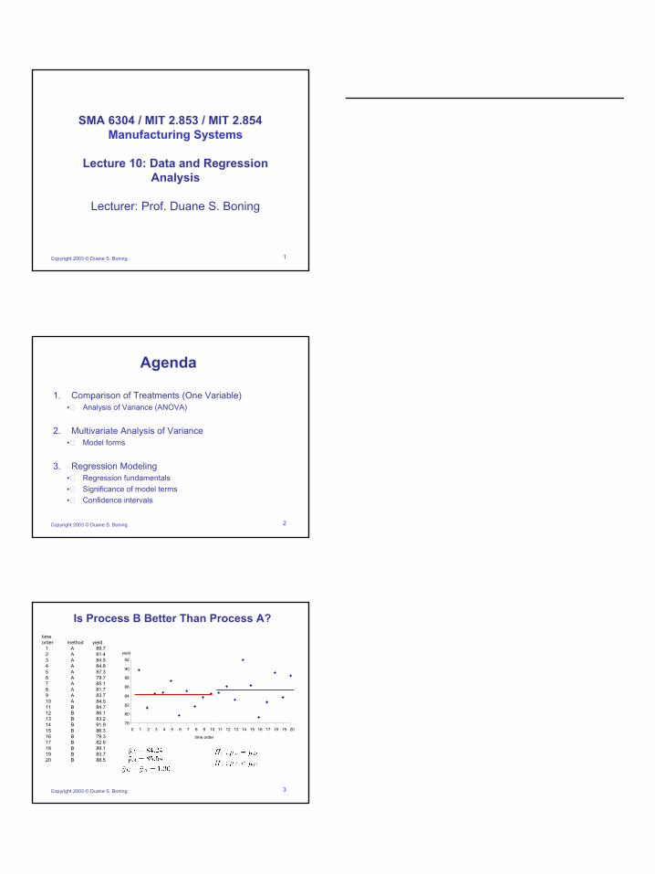
SMA 6304 / MIT 2.853 / MIT 2.854 Manufacturing Systems

Lecture 10: Data and Regression Analysis

Lecturer: Prof. Duane S. Boning

Agenda

1. Comparison of Treatments (One Variable) • Analysis of Variance (ANOVA)

2. Multivariate Analysis of Variance • Model forms

3. Regression Modeling • Regression fundamentals • Significance of model terms • Confidence intervals

Copyright 2003 © Duane S. Boning.

3

ld

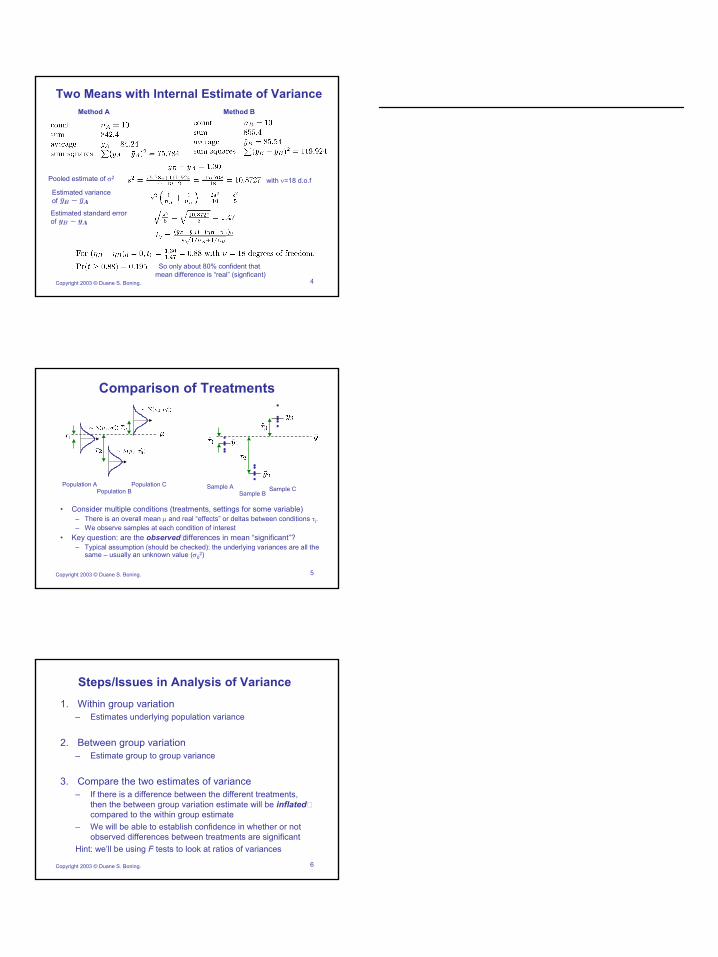
78

80

82

84

86

88

90

92

0 1 2 3 4 5 6 7 8 9 10 11 12 13 14 15 16 17 18 19 20

1 A 2 A 3 A 4 A 5 A 6 A 7 A 8 A 9 A 10 A 11 B 12 B 13 B 14 B 15 B 16 B 17 B 18 B 19 B 20 B


Is Process B Better Than Process A?

yie

time order

time order method yield

89.7 81.4 84.5 84.8 87.3 79.7 85.1 81.7 83.7 84.5 84.7 86.1 83.2 91.9 86.3 79.3 82.6 89.1 83.7 88.5

2

2

4

σ2

of

ν

of


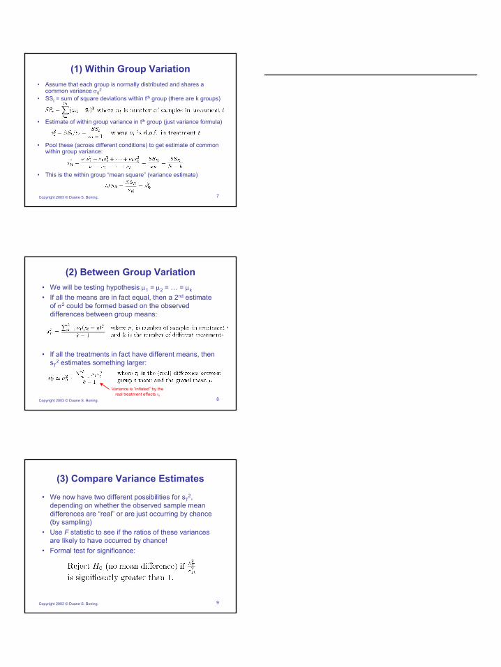
Two Means with Internal Estimate of Variance Method A Method B

Pooled estimate of

Estimated variance

with =18 d.o.f

Estimated standard error

So only about 80% confident that mean difference is “real” (signficant)

Comparison of Treatments

Population A Population C Sample A Sample B

Sample CPopulation B

• Consider multiple conditions (treatments, settings for some variable) – There is an overall mean µ and real “effects” or deltas between conditions τ .i– We observe samples at each condition of interest

• Key question: are the observed differences in mean “significant”? – Typical assumption (should be checked): the underlying variances are all the

same – usually an unknown value (σ02)

Copyright 2003 © Duane S. Boning. 5

Steps/Issues in Analysis of Variance 1. Within group variation

– Estimates underlying population variance

2. Between group variation – Estimate group to group variance

3. Compare the two estimates of variance – If there is a difference between the different treatments,

then the between group variation estimate will be inflated compared to the within group estimate

– We will be able to establish confidence in whether or not observed differences between treatments are significant

Hint: we’ll be using F tests to look at ratios of variances

Copyright 2003 © Duane S. Boning. 6

3

7

• σ0

2

t ithin tth

• i th j

• wi

• i (


(1) Within Group Variation Assume that each group is normally distributed and shares a common variance

• SS = sum of square deviations w group (there are k groups)

Estimate of w thin group variance in t group ( ust variance formula)

Pool these (across different conditions) to get estimate of common thin group variance:

This is the w thin group “mean square” variance estimate)

8

• µ1 = µ2 µk

• nd

of σ2

• sT

2

lτt


(2) Between Group Variation We will be testing hypothesis = … = If all the means are in fact equal, then a 2 estimate

could be formed based on the observed differences between group means:

If all the treatments in fact have different means, then estimates something larger:

Variance is “inf ated” by the real treatment effects

9

• ibiliti T 2,

F

•


(3) Compare Variance Estimates

We now have two different poss es for sdepending on whether the observed sample mean differences are “real” or are just occurring by chance (by sampling)

• Use statistic to see if the ratios of these variances are likely to have occurred by chance! Formal test for significance:

4

10

• F i

• Use F

– i

i αbetter


(4) Compute Significance Level

Calculate observed ratio (w th appropriate degrees of freedom in numerator and denominator)

distribution to find how likely a ratio this large is to have occurred by chance alone

This is our “signif cance level” – If

then we say that the mean differences or treatment effects are s gnificant to (1- )100% confidence or

11

•


(5) Variance Due to Treatment Effects

We also want to estimate the sum of squared deviations from the grand mean among all samples:

12

F0

average

Pr(F0) degrees

of freedomsquaresvariation

Al


(6) Results: The ANOVA Table

mean square

Total about the grand

Within treatments

Between treatments

sum of source of

so referred to as “residual” SS

5

13

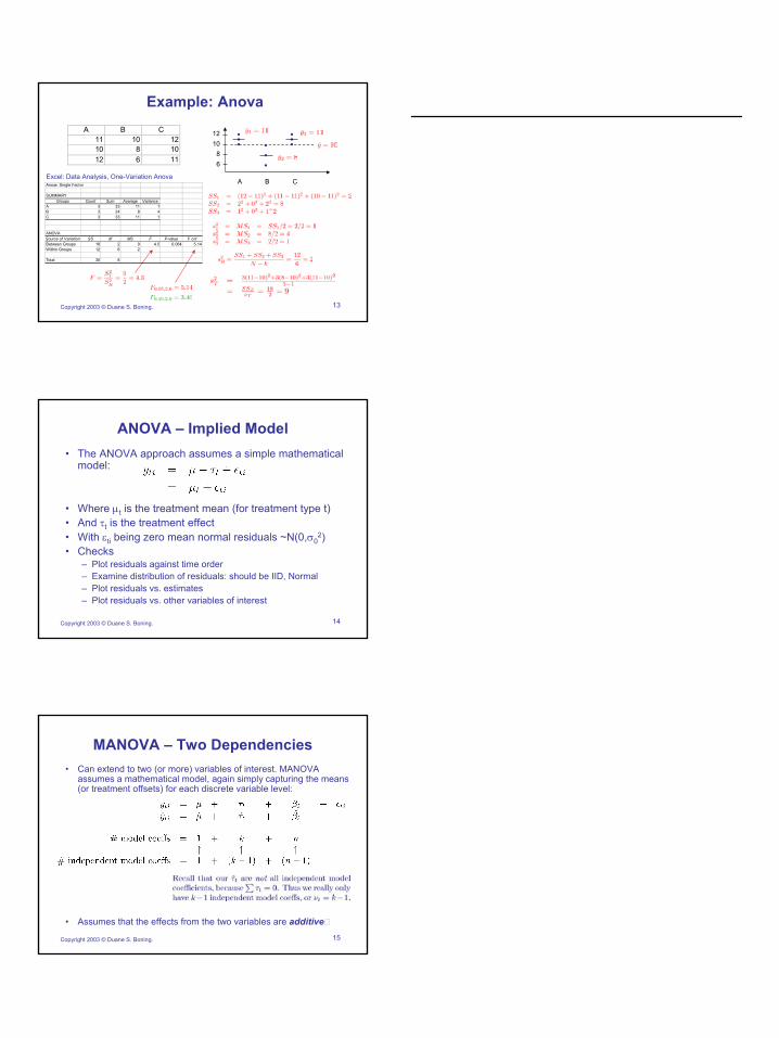
Example: Anova A B C

11 10 10 8 12 6

A B C

6 8

10 12

i

iA 3 1 B 3 8 4 C 3 1

f iati df F it 2 9

Wi 6 2

l 8


12 10 11

Anova: S ngle Factor

SUMMARY Groups Count Sum Average Var ance

33 11 24 33 11

ANOVA Source o Var on SS MS P-value F crBetween Groups 18 4.5 0.064 5.14

thin Groups 12

Tota 30

Excel: Data Analysis, One-Variation Anova

14

• imodel:

• µt • τt • Wi εti σ0

2) •

– – i– –


ANOVA – Implied Model The ANOVA approach assumes a s mple mathematical

Where is the treatment mean (for treatment type t) And is the treatment effect

th being zero mean normal residuals ~N(0,Checks

Plot residuals against time order Exam ne distribution of residuals: should be IID, Normal Plot residuals vs. estimates Plot residuals vs. other variables of interest

15

•

•


MANOVA – Two Dependencies Can extend to two (or more) variables of interest. MANOVA assumes a mathematical model, again simply capturing the means (or treatment offsets) for each discrete variable level:

Assumes that the effects from the two variables are additive

6

16

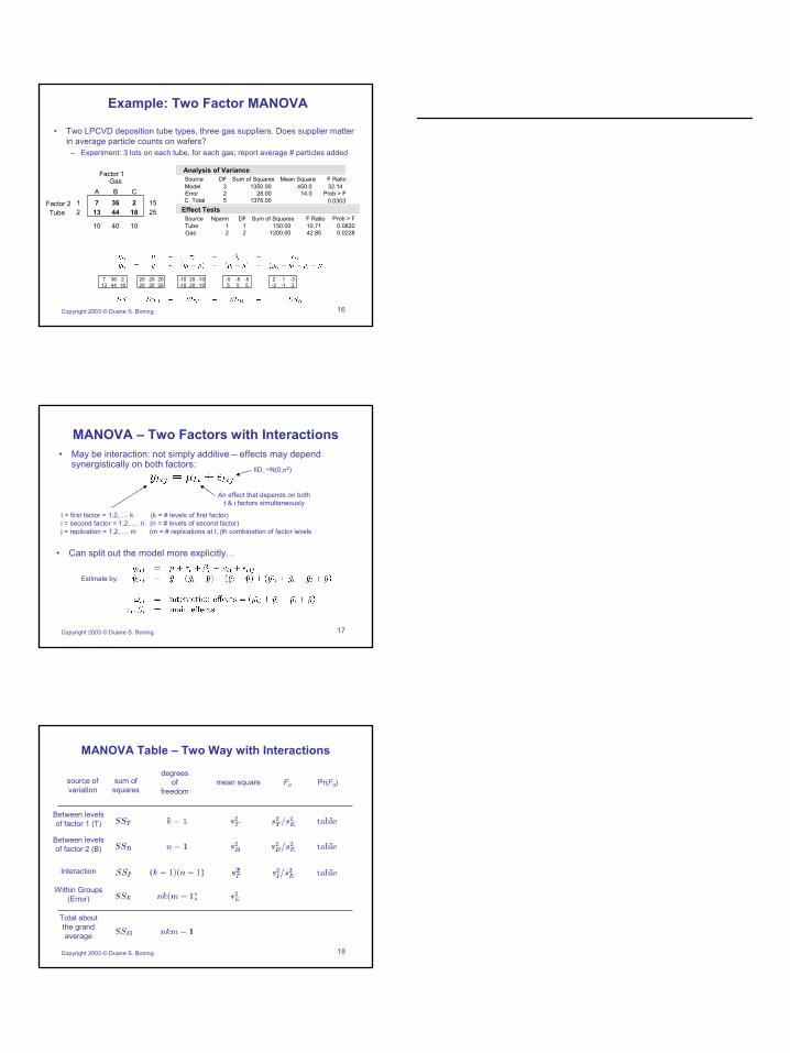
• i li li

–

l

3 2 5

DF

Tube Gas

1 2

1 2

DF

Gas

104010

1523671 Tube

CBA

251844132

3-1-2 -312

20 20

555 -5-5-5

13 2367


Example: Two Factor MANOVA

Two LPCVD deposit on tube types, three gas supp ers. Does supp er matter in average particle counts on wafers?

Experiment: 3 lots on each tube, for each gas; report average # particles added

Model Error C. Tota

Source 1350.00

28.00 1378.00

Sum of Squares 450.0

14.0

Mean Square 32.14 F Ratio

0.0303 Prob > F

Analysis of Variance

Source Nparm 150.00

1200.00

Sum of Squares 10.71 42.85

F Ratio 0.0820 0.0228

Prob > F Effect Tests

Factor 1

Factor 2

-10 20 -10 -10 20 -10

20 20 20 20

18 44

17

•

( σ2)

i

l l )

j

• l


MANOVA – Two Factors with Interactions

Can split out the model more explicitly…

IID, ~N 0,

An effect that depends on both t & factors simultaneously

t = first factor = 1,2, … k (k = # eve s of first factori = second factor = 1,2, … n (n = # levels of second factor) j = replication = 1,2, … m (m = # replications at t, th combination of factor levels

May be interaction: not simp y additive – effects may depend synergistically on both factors:

Estimate by:

18

F0

the grand average

Wi(Error)

Pr(F0) degrees

of


MANOVA Table – Two Way with Interactions

mean square

Total about

thin Groups

Between levels of factor 1 (T)

freedom sum of squares

source of variation

Between levels of factor 2 (B)

Interaction

7

19

2

• 2

– i i j

– (l

• 2

– ii

– i l). ll νR = νD - νT


Measures of Model Goodness – RGoodness of fit – R

Quest on cons dered: how much better does the model do that ust using the grand average?

Think of this as the fraction of squared deviations from the grand average) in the data which is captured by the mode

Adjusted RFor “fair” comparison between models w th different numbers of coefficients, an alternat ve is often used

Think of this as (1 – var ance remaining in the residuaReca

Regression Fundamentals • Use least square error as measure of goodness to

estimate coefficients in a model• One parameter model:

– Model form – Squared error – Estimation using normal equations – Estimate of experimental error – Precision of estimate: variance in b – Confidence interval for β – Analysis of variance: significance of b – Lack of fit vs. pure error

• Polynomial regression


21

•

• l:

• l β wi•

– i inimii

– l


Least Squares Regression

We use least-squares to estimate coefficients in typical regression models One-Parameter Mode

Goa is to estimate th “best” b How define “best”?

That b wh ch m zes sum of squared error between predict on and data

The residua sum of squares (for the best estimate) is

20

8

22

• equations –

l β ile

– il

• – i

2 of σ2


Least Squares Regression, cont.

Least squares estimation via normal

For linear problems, we need not calcu ate SS( ); rather, d rect solution for b is possibRecognize that vector of res duals will be normal to vector of x va ues at the least squares estimate

Estimate of experimental error Assum ng model structure is adequate, estimate s can be obtained:

23

•


Precision of Estimate: Variance in b

We can calculate the variance in our estimate of the slope, b:

• Why?

24

β

• i i α

• – i– i β β

– ion)

i


Confidence Interval for Once we have the standard error in b, we can calculate confidence ntervals to some des red (1- )100% level of confidence

Analysis of variance Test hypothes s: If conf dence interval for includes 0, then not significant

Degrees of freedom (need in order to use t distribut

p = # parameters est mated by least squares

9

25

1 8 9

DF 8836.6440

64.6695 8901.3135

8836.64 8.08

1093.146 io

l

age Zeroed 0

0.500983 0

0.015152 .

33.06

t Ratio . |t|

age 1 1 DF

8836.6440 1093.146 io

0

10

20

30

40

50

ii

0 25 50 75 100

8

22

35

40

57

73

78

87

98

i

i


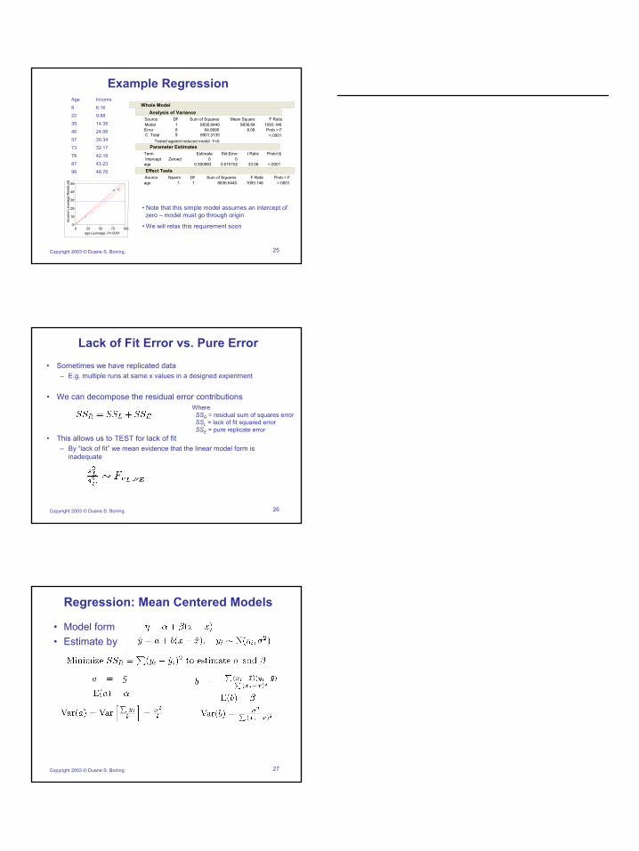
Example Regression

Model Error C. Total

Source Sum of Squares Mean Square F Rat

<.0001 Prob > F

Tested against reduced mode : Y=0


Intercept Term Estimate Std Error

<.0001

Prob>Parameter Estimates

Source Nparm Sum of Squares F Rat<.0001


Whole Model

ncom

e Le

vera

ge R

esdu

als

age Leverage, P<.0001

Age Income

6.16

9.88

14.35

24.06

30.34

32.17

42.18

43.23

48.76

• Note that this s mple model assumes an intercept of zero – model must go through origin

• We w ll relax this requirement soon

26

• –

• i i

• l–

i

SSR iSSL iSSE


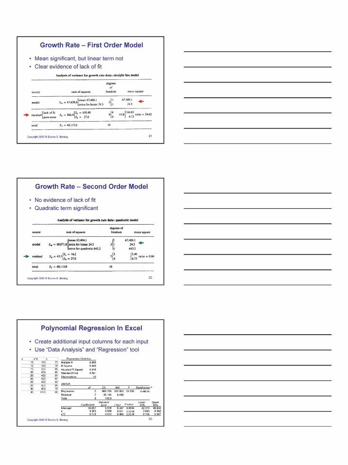
Lack of Fit Error vs. Pure Error Sometimes we have replicated data

E.g. multiple runs at same x values in a designed experiment

We can decompose the res dual error contribut ons

This al ows us to TEST for lack of fit By “lack of fit” we mean evidence that the linear model form is nadequate

Where = res dual sum of squares error = lack of f t squared error = pure replicate error

27

• Model form •


Regression: Mean Centered Models

Estimate by

12

e

34

i ) 10

l

2 7 9

DF

it 3 4 7

DF

x

| Parameter Estimates

x 1 1

1 1

DF


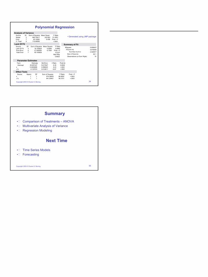
Polynomial Regression

• Generated using JMP package

RSquare RSquare Adj

Root Mean Sq Error Mean of Response

Observat ons (or Sum Wgts

0.936427 0.918264 2.540917

82.1

Summary of Fit

Model Error C. Tota

Source 665.70617 45.19383

710.90000

Sum of Squares 332.853

6.456

Mean Squar 51.5551 F Ratio

<.0001 Prob > F


Lack Of FPure Error Total Error

Source 18.193829 27.000000 45.193829


Mean Square 0.8985 F Ratio

0.5157 Prob > F

0.9620 Max RSq

Lack Of Fit

Intercept

x*x

Term 35.657437 5.2628956 -0.127674

Estimate 5.617927 0.558022 0.012811

Std Error 6.35 9.43

-9.97

t Ratio 0.0004 <.0001 <.0001

Prob>|t

x*x

Source Nparm 574.28553 641.20451


F Ratio <.0001 <.0001


35

• • •

Next Time

• Ti•


Summary Comparison of Treatments – ANOVA Multivariate Analysis of Variance Regression Modeling

me Series Models Forecasting

agenda - mit opencourseware

Documents